Stanford University Energy & Climate...
173
1 | Page Stanford Energy and Climate Plan, October 2009 Stanford University Energy & Climate Plan Rising to the Challenge Through New High Performance Buildings, Innovations in Energy Conservation, & Energy Regeneration October 15, 2009 GREEN BUILDING SHOWCASING INNOVATION WATER CONSERVING PRESCIOUS RESOURCES ENERGY MOVING TO A BRIGHTER FUTURE LAND STEWARDSHIP MAINTAINING NATURAL RICHES TRANSPORTATION GOING THE EXTRA MILE WASTE REDUCING AND RECYCLING
Transcript of Stanford University Energy & Climate...

1 | P a g e Stanford Energy and Climate Plan, October 2009
Stanford University Energy & Climate Plan
Rising to the Challenge
Through New High Performance Buildings, Innovations in Energy Conservation,
& Energy Regeneration
October 15, 2009
GREEN BUILDINGSHOWCASING INNOVATION
WATERCONSERVING PRESCIOUS RESOURCES
ENERGYMOVING TO A BRIGHTER FUTURE
LAND STEWARDSHIPMAINTAINING NATURAL RICHES
TRANSPORTATIONGOING THE EXTRA MILE
WASTEREDUCING AND RECYCLING

2 | P a g e Stanford Energy and Climate Plan, October 2009
Authored by:
Joseph Stagner, Executive Director Fahmida Ahmed, Manager of Sustainability Programs
Department of Sustainability and Energy Management
Stanford University
About Sustainability and Energy Management The Sustainability and Energy Management Department (SEM) consists of Utilities Services, Parking and Transportation Services, and the Office of Sustainability. The department is led by the Executive Director and includes 86 professional, clerical and trades staff. SEM leads the initiative to advance sustainability in campus operations and oversees campus utilities and transportation services. This work includes developing strategic long‐term goals for energy use, greenhouse gas emissions reduction, water use, waste reduction, green building and transportation, as well as developing and administering a communications and community relations program to support the initiative and an evaluation and reporting program to monitor its effectiveness. Sustainable Stanford ‐ the university’s official program on campus sustainability ‐ steers, connects and streamlines campus sustainability work.

3 | P a g e Stanford Energy and Climate Plan, October 2009
Acknowledgements Special thanks to: Mike Goff, Director of Utilities, for great assistance in developing long term energy supply strategies, providing professional internal and external peer reviews, and adeptly coordinating efforts across all engineering disciplines to assure comprehensive and consistent planning. Robert Reid, Manager of the Stanford Central Energy Facility in the Utilities Department for critical contributions in advanced energy supply modeling and planning. Dean Murray, Manager of Stanford Steam and Chilled Water Distribution Systems in the Utilities Department for development of conceptual plans for conversion of the campus steam distribution system to hot water and preparation of long term capital forecasts for all options. The support and guidance of the Greenhouse Gas Reduction Blue Ribbon Task Force was integral to the development of this Plan:
Lynn Orr, Keleen & Carlton Beal Professor in Petroleum Engineering & Director of the Precourt Institute for Energy
Jim Sweeney, Professor of Management Science & Engineering and Senior Fellow at the Woods Institute and, by courtesy, at the Hoover Institution and Director, Precourt Institute for Energy Efficiency
Larry Goulder, Shuzo Nishihara Professor in Environmental & Resource Economics John Weyant, Professor (Research) of Management Science and Engineering Roland Horne, Thomas Davies Barrow Professor in the School of Earth Sciences, and Joseph Stagner, Executive Director of Sustainability & Energy Management
The Plan greatly benefited from insights and advice from: Gil Masters, Emeritus Faculty, Civil and Environmental Engineering Clyde ‘Bob’ Tatum, Emeritus Faculty, Civil and Environmental Engineering Jeff Koseff, William Alden Campbell & Martha Campbell Professor‐ School of Engineering and Perry
L. McCarty Director of the Woods Institute & Senior Fellow at FSI Barton H “Buzz” Thompson, Robert E. Paradise Professor of Natural Resources Law, Senior Fellow
and Perry L. McCarty Director of the Woods Institute Thomas Fenner, Deputy General Counsel, Office of the General Counsel The Plan is also built upon contributions from the following staff in the Sustainability & Energy Management (SEM) Department: Susan Kulakowski, Demand‐Side Energy Manager, SEM Scott Gould, Senior Energy Engineer, Utilities, SEM Richard Bitting, Power Systems Manager, Utilities, SEM Joyce Dickerson, Director of Sustainable Information Technology, SEM Tom Zigterman, Associate Director and Civil Infrastructure Manager, SEM Brodie Hamilton, Director, Parking and Transportation, SEM Elsa Baez, Staff Assistant to SEM, SEM

4 | P a g e Stanford Energy and Climate Plan, October 2009
Table of Contents
Foreword: Harnessing Regeneration Potential at Stanford .................................................................. 8
Executive Summary .............................................................................................................................................. 9
Chapter 1: The Need for Climate Action ..................................................................................................... 12
Major Events in Global Climate Action.......................................................................................................... 12 Major Events in National Climate Action ..................................................................................................... 13 Major Events in State Climate Action ............................................................................................................ 16 Early Climate Action at Stanford University ............................................................................................... 18
Chapter 2: Principles, Approach and Processes ..................................................................................... 20
Guiding Principles ................................................................................................................................................. 20 Energy and Climate Plan Process .................................................................................................................... 21 Summary of Steps .................................................................................................................................................. 21
Chapter 3: Stanford Emissions & Growth .................................................................................................. 25
Protocols for the Emissions Inventory ......................................................................................................... 25 Scope Descriptions ................................................................................................................................................ 26 Stanford University Emissions Inventory ................................................................................................... 26 Campus Growth and Emissions Trends ........................................................................................................ 28 A Balanced Approach to Finding Solutions ................................................................................................. 31
Chapter 4: Minimizing Energy Demand in New Buildings .................................................................. 32
New Building Standards ..................................................................................................................................... 32 High Performance Buildings at Stanford ..................................................................................................... 35 Jasper Ridge Field Station (2005) ................................................................................................................... 35 Carnegie Global Ecology Research Center (2007) ................................................................................... 35 Knight Management Center (2011) ............................................................................................................... 38 The Green Dorm (2014) ...................................................................................................................................... 39
Chapter 5: Reducing Energy Use in Existing Buildings ......................................................................... 40
Existing Energy Conservation Initiatives ..................................................................................................... 40 New Energy Conservation Initiatives ............................................................................................................ 42 Energy Conservation from Individual Behavior (in pilot) .................................................................... 46
Chapter 6: Energy Supply Options ................................................................................................................ 47
Energy Supply Options ........................................................................................................................................ 47 Model Variables ...................................................................................................................................................... 55 Model Analysis ........................................................................................................................................................ 59 Summary of Model Results ................................................................................................................................ 77

5 | P a g e Stanford Energy and Climate Plan, October 2009
Chapter 7: Comprehensive Energy Plan .................................................................................................... 82
Emissions Reduction in ‘Metric Tons’ ........................................................................................................... 82 Emissions Reduction in ‘Dollars’ ..................................................................................................................... 87 The Total Business Case for Climate Action in ‘Dollars and Tons’ .................................................... 89
Chapter 8: Role of Carbon Instruments ..................................................................................................... 91
Definition and Description of Various Carbon Instruments ................................................................ 91 Legitimacy Requirements for RECs and Offsets ........................................................................................ 93 California Regulation – AB‐32 Scoping Plan Implementation ............................................................. 94 Risks and Uncertainties with Carbon Instruments .................................................................................. 96 Cost .............................................................................................................................................................................. 96 Standards .................................................................................................................................................................. 98 The Relationship between Regulations ........................................................................................................ 99 Perception ................................................................................................................................................................. 99 Recommendations Regarding Carbon Instruments ............................................................................. 100
Chapter 9: Findings & Recommendations .............................................................................................. 102
Energy Conservation Will Be Outpaced by Growth ‐ Energy Supply Changes Are Key ......... 102 Changing from Cogeneration to Regeneration Offers Many Advantages .................................... 102 Stanford Can Leverage the Business Case in Climate Action ............................................................ 104 Remain Vigilant of Carbon Instruments Development ....................................................................... 104 Investigate Renewable Energy ...................................................................................................................... 105
Appendix A: Stanford Emissions Inventory ............................................................................................ 107
Appendix B: Initial List of GHG Reduction Options .............................................................................. 121
Appendix C: Various Emissions Reduction Goals .................................................................................. 124
Appendix D: (reserved) ................................................................................................................................. 128
Appendix E: Campus Utilities Growth Projections ............................................................................... 129
Appendix F: Heat Recovery Potential at Stanford ................................................................................. 132
Appendix G: Benefits of Converting Steam Distribution to Hot Water ......................................... 136
Appendix H: Data Set of Steam and Chilled Water Production Figures ........................................ 139
Appendix I: Variables and Ranges used in Modeling ........................................................................... 140
Appendix J: Advanced “Parallel” Modeling ............................................................................................. 144
Appendix K: Comparison of Efficiency CHP vs SHP vs Heat Recovery ......................................... 146
Appendix L: Cost comparison of supply options with direct emissions reduction .................. 148
Appendix M: Cost Comparison of Supply Options with Indirect Emissions Reduction .......... 150
Appendix N: Detailed Model Results – other six bins ......................................................................... 156
Appendix O: Peer Review Consultants’ Reports ................................................................................... 163
Appendix P: Evaluation of Energy Price Risk and Budget Stability ............................................... 164

6 | P a g e Stanford Energy and Climate Plan, October 2009
Appendix Q: Early Action on Carbon Instruments at Other Academic Institutions ................. 166
Appendix R: Energy Systems Capital Investment Schedules ............................................................ 167
Appendix S: Renewable Energy Transmission Initiative Report .................................................... 168
Report References ............................................................................................................................................ 169

7 | P a g e Stanford Energy and Climate Plan, October 2009
List of Figures Chapter 3 Figure‐3.1: Stanford University Emissions Inventory 2007 Figure 3‐2: Stanford University Space Growth Projections Figure 3‐3: GHG Trends and Target Considerations Chapter 6 Figure 6‐1: Business As Usual CHP Figure 6‐2: Combined Heat and Power Figure 6‐3: Separate Heat and Power Figure 6‐4: Regeneration Scheme Figure 6‐5: Heat Recovery Potential Figure 6‐6: Overall Comparative CHP, SHP, and Regeneration Efficiency Figure 6‐7: CHP v Regeneration Efficiency w 39% CCGT Power Figure 6‐8: CHP v Regeneration Efficiency w 54% CCGT Power Figure 6‐9: Variables Bins Used for Energy and Climate Action Modeling Figure 6‐10: Comparison of Supply Options ‐ Medium gas cost Figure 6‐11: Comparison of Supply Options ‐ low gas cost Figure 6‐12: Comparison of Supply Options ‐ high gas cost Figure 6‐13: Cumulative Cash Flows‐ No GHG Restrictions Figure 6‐14: Annual Cost Difference: BAU v New Options‐ No GHG Restrictions Figure 6‐15: Cumulative Cash Flows‐ 50% Direct GHG Reduction Figure 6‐16: Annual Cost Difference: BAU v New Options‐ 50% Direct GHG Reduction Figure 6‐17: Energy Supply Option Costs‐ Direct GHG Reductions Figure 6‐18: Campus Domestic Water Use Forecasts Chapter 7 Figure 7‐1: The Emissions Reduction Wedge Diagram Figure 7‐2: Summary of Costs and GHG Reduction Options Figure 7‐3: GHG Reductions and Costs

8 | P a g e Stanford Energy and Climate Plan, October 2009
Foreword: Harnessing Regeneration Potential at Stanford
Energy can neither be created nor destroyed, but only changed from one form to another.
‐ First law of thermodynamics
There is a lot of energy changing from one form to another at Stanford University every day, and most of it is natural gas being changed to electricity and heat in the campus cogeneration facility. But increasing energy costs and climate impacts from burning fossil fuel compel us to find new methods of energy supply, ones inspired not by the restrictions of the laws of thermodynamics but instead by their possibilities. One such method is Regeneration through heat recovery.
Stanford University is served by a district heating and cooling system powered by a central energy facility (CEF). In the heating process heat is produced at the CEF and transported to buildings via the steam system for heating and hot water use. In the cooling process unwanted heat is collected from buildings and transported by the chilled water system to the CEF where it is discarded to the atmosphere via evaporative cooling towers.
While much heating is done in winter and much cooling in summer, any overlap of the two provides an opportunity for recovery and reuse of heat energy that is normally discarded to the atmosphere at considerable added energy and water expense to operate chillers and cooling towers. At Stanford the heating and cooling overlap is about 70%‐ a potential to satisfy half of the university’s heating demands and reduce GHG emissions by 30%‐ while also saving over $639 million between 2010 and 2050 versus continued use of a third party cogeneration energy supply.
An energy supply system that uses fossil fuel to produce electricity and then recovers waste heat from the combustion process for heating is known as combined heat and power, or Cogeneration. An energy supply system that allows flexibility in the method of electricity generation, such as from renewable sources, and which recovers waste heat produced freely by the environment rather than relying on fossil fuel combustion can be thought of as Regeneration.
The use of Cogeneration has been a sound practice at Stanford over the past two decades based on the economics of energy and known environmental impacts of the time. However, new information about the impact of fossil fuel use on climate change has come to light and energy costs have changed significantly, leading the university to move beyond cogeneration to Regeneration as our next step in the pursuit of an efficient and sustainable energy supply.

9 | P a g e Stanford Energy and Climate Plan, October 2009
Executive Summary Climate change is one of the most significant global socioeconomic challenges for our generation, yet it also provides opportunity for Stanford University to develop innovative solutions and provide leadership through research, teaching, outreach, and the operation of its own campus. Over the past 20 years Stanford has done much to reduce climate impacts. To reduce energy demand the university has set strong new building energy efficiency standards and has employed energy metering at all its facilities for over ten years to understand how and where energy is being used. That information has been used to support strong energy‐efficiency programs including the Energy Conservation Incentive Program (ECIP), the Energy Retrofit Program (ERP), the Major Capital Improvement Program, and the Advanced Building Management program. Most recently, new innovative conservation initiatives have been launched to stem rapid energy demand growth in the high tech areas of Information Technology and Cold Storage of medical and biological samples. On the energy supply side the campus has used natural gas fired cogeneration to provide its energy since the late 1980’s. Gas fired cogeneration is one of the cleanest and most efficient forms of fossil fuel fired energy production that is just now being adopted by others and promoted as a key strategy in California’s GHG reduction plans. But while continuous improvement in new building energy efficiency and conservation in existing buildings remains a cornerstone of our long term energy and climate action strategy, a shift away from a 100% reliance on fossil fuel is now prudent due to changes in energy costs and climate impacts from GHG emissions. Purpose The purpose of this Energy and Climate Plan is to outline a comprehensive, practical and cost effective plan for reducing Stanford’s greenhouse gas emissions through the way we construct and operate our facilities and supply energy to them. Serving as a blueprint for implementation, this plan: demonstrates long term cost effectiveness and sustainable natural resource use; guides development of critical campus infrastructure; and reduces the economic and regulatory risk in Stanford’s long term energy supply.
(Image: Stanford University campus from above, Jawed Karim.)

10 | P a g e Stanford Energy and Climate Plan, October 2009
Results In summary, this plan covers the period 2010 to 2050 and provides:
• Cost savings of $639 million over the business‐as‐usual case of third party cogeneration; • Reduction in greenhouse gas emissions of 20% below 1990 levels by 2020; • Opportunities for even higher emissions reductions by 2050 should regulatory and
economic conditions allow; • Total campus water savings of 18% over current projections; • Modestly lower campus land use by central energy facilities than business‐as‐usual; • Flexibility for adoption of new energy supply technologies and innovations that may
develop to further decrease campus energy and water use.
Implementation of the plan will require: • Achievement of new building energy efficiency standards of 30% below code; • Continuance and expansion of energy conservation in existing buildings; • Moving from a third party owned and operated combined heat and power (CHP)
cogeneration plant to a university owned and operated separate heat and power (SHP) plant with heat recovery;
• Major changes to campus infrastructure, most notably conversion of the campus steam distribution system to hot water;
• Capital investment of $69 million or 13% more than the business‐as‐usual case between 2010 and 2050 (cost included in the savings figure cited above).
Implementation of the plan does not require:
• Direct Access to state electricity markets, though this would likely increase cost savings; • Use of carbon instruments such as Renewable Energy Credits (RECs) or carbon offsets; • Regulatory approvals in excess of business‐as‐usual.
A full range of potential campus energy supply strategies, growth scenarios, and future energy prices were examined in developing this plan. Multiple long term energy models were used and internal and professional third party external peer reviews were performed to confirm the findings. Energy supply options that were considered include:
• Business‐as‐usual long term third party owned and operated gas fired cogeneration; • Campus owned and operated gas fired cogeneration plant; • Campus owned and operated boilers and chillers plant with imported electricity; • Campus owned and operated boilers, chillers, and heat recovery plant with imported
electricity (the recommended option). Campus growth scenarios considered (consistent with the 2008 Sustainable Development Study):
• Minimal growth (115,000 gsf/year) • Moderate growth (200,000 gsf/year) • Aggressive growth (300,000 gsf/year)

11 | P a g e Stanford Energy and Climate Plan, October 2009
Energy prices tested:
• Natural Gas: Department of Energy January 2009 long range forecast ±20% • Imported Electricity: PG&E projected rates ±10% to reflect influence of natural gas prices • Renewable Electricity: $90/MWh to $140/Mwh
While the cost savings figures cited above represent the middle case of moderate campus growth and medium expected natural gas and electricity prices, the full range of potential outcomes for the proposed heat recovery plan across all growth and energy price scenarios is a net present value savings ranging from $217 million to $1.1 billion and GHG reductions of 74% to 80% below the 2000 baseline. In all foreseeable operating scenarios, the recommended heat recovery option costs less, consumes fewer natural resources, and generates the least amount of greenhouse gas. Caveats It should be noted that if GHG emissions are allowed to grow without restriction due to campus decision and/or the absence of direct regulatory control a Stanford owned cogeneration plant may provide the lowest cost, though it would come with significant economic and regulatory risk. Furthermore it should be noted that the economic benefits of a heat recovery strategy could take about ten years or so to materialize under the middle case scenario. This could occur if carbon emissions are not monetized by regulatory actions such as cap and trade or fuel price surcharges, because in the early years the cogeneration option takes full advantage of high but steadily declining GHG limits and emits far more GHG than the heat recovery option without penalty. It could also occur because the capital cost for the heat recovery option is ‘front end loaded’ compared to the other options. The major cost of the heat recovery option is an estimated $120 million for the conversion of the steam distribution and condensate return pipelines to hot water. If this cost were spread over the 80 year expected life of the improvement rather than the 40 year financing period suitable for the life expectancy of a cogeneration plant it would erase any short term cash flow advantage the cogeneration option may offer. In contrast, as compared to continuance of a business‐as‐usual third party cogeneration arrangement the heat recovery option pays back within just a few years. The Regeneration strategy described in the Foreword and explained more in Chapter 6 will advance Stanford’s place at the forefront in sustainability through innovation, adept business practice, and leadership by example. It offers Stanford the greatest flexibility to develop and deploy additional innovations in energy conservation, efficiency, and alternative energy supply to achieve additional cost savings, GHG reduction, and water savings. Also, by significantly decoupling the campus energy supply from fossil fuel, greater operating budget stability is provided and economic, regulatory and public relations risks are reduced.

12 | P a g e Stanford Energy and Climate Plan, October 2009
Chapter 1: The Need for Climate Action
Stabilization and reversal of greenhouse gas (GHG) emissions into the atmosphere from human activity is a challenge that seeks solutions in the areas of both research and implementation of research findings. The sense of urgency is set by the climate science. The UN Intergovernmental Panel on Climate Change (IPCC) has found that developed countries, as a group, need to reduce emissions by 25–40 per cent by 2020, on a 1990 baseline, in order to contain warming to 2.0–2.4 degrees. This standard translates to about a 50% reduction in greenhouse gas emissions from 2000 levels by 2050, in order to restrict global warming to what are believed to be manageable levels. 1 Most widely recognized GHG goals specify both interim (2010 to 2020) and long term (2050) reductions. Such a significant reduction worldwide will require strong carbon regulations and effective technology implementation globally and locally – an opportunity for any entity to take local action within the framework of a global regulatory and economic framework. This chapter outlines the key events in climate action globally and locally, to contextualize Stanford University’s approach towards its Energy and Climate Plan.
Major Events in Global Climate Action The following key steps have shaped and formed climate action globally and locally, and have informed Stanford’s decisions and analytical framework for climate action planning. UNFCCC: International efforts to address climate change began in 1992 with the United Nations Framework Convention on Climate Change (UNFCCC). The UNFCCC established the aim to stabilize atmospheric GHG concentrations “…at a level that would prevent dangerous anthropogenic interference with the climate system” and affirmed several important principles of environmental law, including common but differentiated responsibility, sustainable development, and the precautionary principle (UNFCCC, 1992).
The Kyoto Protocol: The Kyoto Protocol quantified UNFCCC’s objective by establishing specific targets and timetables for GHG reduction. Adopted in 1997, the Kyoto Protocol set binding targets
1 Ref: IPCC http://www.ipcc.ch/index.html, (Box 13.7 in the IPCC Fourth Assessment Report)

13 | P a g e Stanford Energy and Climate Plan, October 2009
for developed countries to reduce GHG emissions (7% below 1990 levels for the U.S., 8% for Europe) by the 2008‐12 commitment period, and (consistent with the principle of common but differentiated responsibility) left the issue of developing country commitments to the post‐2012 commitment period (UNFCCC, 1997).
Participation in the Kyoto Protocol Signed and ratified Signed, ratification pending Signed, ratification declined Source: http://en.wikipedia.org/wiki/Kyoto_Protocol
In order to meet its Kyoto targets, the European Union (EU) established the European Union Greenhouse Gas Emission Trading Scheme (EU ETS). It is the largest multi‐country, multi‐sector greenhouse gas emission trading scheme in the world (European Commission, 2007). The Clean Development Mechanism (CDM) Standards is a flexible compliance mechanism of the Kyoto Protocol; CDM supports offset projects in developing countries. Sanctioned as a way for governments and private companies to earn carbon credits, CDM produced offsets, which can be traded on a marketplace, have stringent standards with strict ‘additionality’ requirements. However, despite the stringency, loopholes in the carbon credit protocols/standards have caused undesired market behavior. (See Chapter 8 for more on choice of CDM offset projects).
Major Events in National Climate Action
The U.S. is party to the UNFCCC, but not to its implementing treaty, the Kyoto Protocol. Following the issuance of the Byrd‐Hagel Resolution, expressing the Senate’s concern over the potential negative economic impacts of emissions restrictions and its objection to participating in a treaty that did not also cover developing countries, the executive administration did not send the Kyoto Protocol to the Senate for ratification. The administration did not support the Kyoto Protocol and opposed a mandatory GHG emissions reductions commitment. However, a variety of significant efforts are currently underway to aid the process of emissions reduction. Like pieces of a puzzle, each of these elements plays an important role in energy and climate efforts now more widely supported in the executive and legislative branches of government.

14 | P a g e Stanford Energy and Climate Plan, October 2009
Voluntary Programs: While not supporting mandatory reduction requirements the executive administration did establish GHG emissions intensity targets, voluntary programs (for example, the EPA’s Climate Leaders and Energy Star), and international partnerships without mandatory enforcement mechanisms (for example, the Asia‐Pacific Partnership on Clean Development and Climate).
Source: Courtesy of Jacobs http://www.jacobs.com/
Western Climate Initiative: The Western Climate Initiative, launched in February 2007, is a collaboration of seven U.S. governors and four Canadian Premiers. Created to identify, evaluate, and implement collective and cooperative ways to reduce greenhouse gases in the region, the partnership has provided a great deal of insight into a regional, market‐based cap and trade system. Regional Greenhouse Gas Initiative (RGGI): Signed in 2005, the Regional Greenhouse Gas Initiative (RGGI) is the first mandatory, market‐based effort in the United States to reduce greenhouse gas emissions. Ten Northeastern and Mid‐Atlantic states will cap and then reduce CO2 emissions from the power sector 10% by 2018. “States will sell emission allowances through auctions and invest proceeds in consumer benefits: energy efficiency, renewable energy, and other clean energy technologies. RGGI will spur innovation in the clean energy economy and create green jobs in each state.” http://www.rggi.org/home

15 | P a g e Stanford Energy and Climate Plan, October 2009
Midwest Greenhouse Gas Reduction Accord (MGA): Nine Midwestern governors and two Canadian premiers have signed on to participate in or observe the Midwest Greenhouse Gas Reduction Accord (Accord), as first agreed to in November 2007 in Milwaukee, Wisconsin. As the most coal‐dependent region in North America, the Midwest also has great renewable energy resources and opportunities that allow it to take a lead role in addressing climate change. Through the Accord, these governors agreed to establish a Midwestern greenhouse gas reduction program to reduce greenhouse gas emissions in their states, as well as a working group to provide recommendations regarding the implementation of the Accord. http://www.Midwest ernaccord.org/ Supreme Court Ruling that CO2 is a pollutant: On April 2, 2007, the Supreme Court handed down Massachusetts v. EPA, its first pronouncement on climate change. The Court ruled that carbon dioxide is a pollutant under the Federal Clean Air Act, and said the EPA “abdicated its responsibility” under the Clean Air Act in deciding not to regulate carbon dioxide. The Court's decision leaves EPA with three options under the section: find that motor vehicle greenhouse gas emissions may "endanger public health or welfare" and issue emission standards; find that they do not satisfy that prerequisite; or decide that climate change science is so uncertain as to preclude making a finding either way. The decision also has implications for other climate‐change related litigation, particularly a pending suit seeking to compel EPA regulation of greenhouse gas emissions from stationary sources of emissions. http://opencrs.com/document/RS22665 US Mayors Climate Protection Agreement: Committed to promoting more action at the local level, on February 16, 2005 (the day Kyoto Protocol became effective for 141 ratified countries), Seattle Mayor Greg Nickels launched this initiative to advance the goals of the Kyoto Protocol through leadership and action by at least 141 American cities. By June 2005, 141 mayors had signed the Agreement – the same number of nations that ratified the Kyoto Protocol. Under the Agreement, participating cities commit to take the following three actions: 1) strive to meet or beat the Kyoto Protocol targets in their own communities, through actions ranging from anti‐sprawl land‐use policies to urban forest restoration projects to public information campaigns; 2) Urge their state governments, and the federal government, to enact policies and programs to meet or beat the target suggested for the United States in the Kyoto Protocol – a 7% reduction from 1990 levels by 2012; and 3) Urge the U.S. Congress to pass the bipartisan greenhouse gas reduction legislation, which would establish a national emission trading system. http://usmayors.org/climateprotection/agreement.htm

16 | P a g e Stanford Energy and Climate Plan, October 2009
Academic Institutions – American Colleges and Universities Presidents Climate Commitment (ACUPCC): In late 2006, a group of college and university presidents launched a high‐visibility effort to address global warming by making a joint commitment to reduce GHG emissions at their institutions, ultimately leading to climate neutral campuses. The effort is modeled after the U.S. Mayors Climate Protection Agreement. After program and planning sessions among a group of college and university presidents and their representatives at the AASHE conference in October 2006 at Arizona State University, 12 presidents agreed to become Founding Members of the Leadership Circle and launch the American College and University Presidents Climate Commitment. The current membership has exceeded 600 universities. Stanford University is not yet a signatory but anticipates a decision on this based on the final decisions on the Energy and Climate Action Plan. http://www.presidentsclimatecommitment.org/
Major Events in State Climate Action
GHG regulation in the United States is being pioneered by California. As the 6th largest economy and 12th largest GHG emitter in the world, California has the leadership and legislative potency to define an emissions management scheme for the entire nation. Key actions include: Executive Order S305: In 2005, California Governor Arnold Schwarzenegger signed Executive Order S‐3‐05, committing California to specific emissions reduction targets and creating a Climate Action Team to help implement the directives. Under this order, three specific targets have been established: 2000 levels by 2010, 1990 levels by 2020, and 80% below 1990 levels by 2050. Assembly Bill 32 (AB32): California demonstrated national and international leadership in climate action by passing Assembly Bill 32 (AB‐32) in 2006, authored by Fran Paley and Fabian Nunez. AB‐32 Global Warming Solutions Act of 2006 codified the middle target of Executive Order S‐B‐05 and requires the state of California to reduce its emissions to 1990 levels by 2020. State Bill Assembly Bill 375 (SB375): To tackle issues around smart land use and transportation, SB 375, a bill in the California State Senate authored by Senator Darrell Steinberg, was passed in 2007 to compel local planning agencies to make planning choices that reduce Vehicle

17 | P a g e Stanford Energy and Climate Plan, October 2009
Miles Traveled (VMT). Governor Schwarzenegger signed SB 375, building on AB‐32 by adding the nation's first law to control greenhouse gas emissions by curbing sprawl. AB32 Implementation: The California Air Resources Board (The Board) finalized in early December 2008 a scoping plan to fulfill the key provisions of AB‐32 to establish a statewide GHG emissions cap for 2020 based on 1990 emission levels. The Scoping Plan suggests an emissions cap and trade program as a major and viable emissions reduction option; it recommends that California implement a cap and trade program that links with other Western Climate Initiative (WCI) partner programs to create a regional market system. “This system would require California to formalize enforcement agreements with its WCI partner jurisdictions for all phases of cap and trade program operations, including verification of emissions, certification of offsets based on common protocols, and detection of and punishment for non‐compliance.” Senate Bill 1368: On September 29, 2006, Governor Schwarzenegger signed into law Senate Bill 1368 (Perata, Chapter 598, Statutes of 2006). The law limits long term investments in baseload generation by the state's utilities to power plants that meet an emissions performance standards (EPS) jointly established by the California Energy Commission and the California Public Utilities Commission. The growing awareness of climate change and the need for timely action is converging with the increased national scope of regulatory and business action. There are regulatory solutions on the horizon; local governments and businesses are realizing economic gain from tighter resource management, and the dependence on fossil fuel is now politically unpopular. However, while the momentum for climate action increases it is uncertain whether timely action will be taken that will actually and cumulatively bring CO2 concentration down to a steady state.
Many institutions, including Stanford University, however, are compelled to act now to meet the timetable determined by the earth’s atmospheric balance. Often referred to as a long term problem that now requires a short term solution, climate change poses the difficult task of innovating and implementing new solutions in parallel.

18 | P a g e Stanford Energy and Climate Plan, October 2009
Early Climate Action at Stanford University
In Academics On the academic side, Stanford researchers have been engaged since the 1970s in seeking solutions through participation on the Intergovernmental Panel on Climate Change and through work on numerous initiatives, such as the Global Climate and Energy, the Woods Institute for the Environment, the Precourt Institute, and the Program on Energy and Sustainable Development. The Initiative on the Environment and Sustainability promotes interdisciplinary research and teaching involving all seven of Stanford’s schools, centers, institutes and programs across campus, in recognition of the fact that solutions to complex challenges demand collaboration across multiple fields. The University’s schools offer an array of courses and degree programs focused on environmental sustainability.2 Stanford introduced the pioneering I‐Earth (Introduction to the Earth) curriculum in Fall 2006 to help students develop an interdisciplinary understanding of the planet and the intersections of its natural and human systems. 3 The University has formed the interdisciplinary Woods Institute for the Environment to coordinate the various environmental academic initiatives. The Woods Institute harnesses the expertise and imagination of University scholars to develop practical solutions to the environmental challenges facing the planet ‐‐ from climate change to sustainable agriculture to conservation. The Institute brings together prominent scholars and leaders from business, government and the nonprofit sector through a series of Uncommon Dialogues and Strategic Collaborations designed to produce pragmatic results that inform decision‐makers. In Campus Operations On the operations side, Stanford has employed energy metering of all its facilities to understand how and where energy is being used and has pursued strong energy‐efficiency programs for over ten years. These programs include (more detailed discussion in Chapter 5):
• Energy Conservation Incentive Program (ECIP) that provides financial incentives for electricity conservation in buildings
• Energy Retrofit Program (ERP) that reinvests savings in utility bills in additional energy conservation projects such as HVAC replacement, lighting upgrades, etc.
2 The Stanford Environmental Portal (http://environment.stanford.edu/cgi-bin/index.php) provides extensive information about environmental research and education across the campus. 3 (http://pangea.stanford.edu/courses/i-earth/index.html)

19 | P a g e Stanford Energy and Climate Plan, October 2009
• Major Capital improvement program for major retrofits of the most energy intensive campus buildings
• Advanced Building Management program for optimizing building system operating
schedules to occupancy patterns, detecting energy leaks, and continuous commissioning of building systems
• Cogeneration – While Stanford now plans to advance beyond cogeneration to Regeneration
(see Foreword), it has for the past twenty years employed one of the most efficient forms of energy supply in natural gas‐fired cogeneration for virtually all its energy. Although gas‐fired cogeneration does emit GHGs, it is one of the most efficient forms of fossil fuel‐based energy production. So much so that both the European Union4 and the State of California (http://www.arb.ca.gov/cc/scopingplan/document/draftscopingplan.htm) have adopted policies and regulations favoring increased use of cogeneration as a means of achieving overall GHG reductions. Gas‐fired cogeneration can be a good solution for energy and climate action in many instances, however, at Stanford the use of Regeneration offers superior benefits and does not commit the university to the continuation of a long term fossil fuel‐fired generation source such as cogeneration.
Stanford has done much to reduce GHG impacts from its operations to date. However, these efforts have largely been guided by general principles and specific policies rather than a detailed plan covering all sectors of endeavor. Given the challenges and scale of resources required for this effort, the university embarked on development of a formal energy and climate action plan in November of 2007. As described in Chapter 2, the campus administration decided to focus the climate plan on the energy sector, in order to develop solutions for the activities that contribute to the majority of GHG emissions. The university will proceed with emissions reduction from transportation and other sectors in the upcoming years.
4 EU Directives on Cogen 2004/8/EC & 2007/74/EC , at <http://europa.eu/scadplus/leg/en/lvb/l27021.htm>

20 | P a g e Stanford Energy and Climate Plan, October 2009
Chapter 2: Principles, Approach and Processes The previous chapter discussed Stanford’s commitment to climate action, in the context of state, national, and international developments. This chapter outlines the key principles, planning and analysis approach used to develop Stanford’s Energy and Climate plan.
Guiding Principles Stanford’s principles for energy and climate plan are:
1. Holistic and Long Term Approach — Recognize that emissions reduction may come from a number of areas in campus facilities design, construction, operations, and maintenance, affecting a diverse group of students, staff, and faculty across all academic and administrative departments as well as the surrounding community; recognize that Stanford has to operate within the broader context of energy infrastructure, emissions reduction, and regulation; recognize that both short and long term improvements are needed and that many upcoming decisions on long‐lived buildings and infrastructure will have long range impacts that must be considered before those decisions are made.
2. Vision — Apply Stanford’s intellectual and financial resources to provide leadership in climate change solutions, even if these efforts may differ from popular perceptions of how to pursue GHG reduction or are greater than what governmental regulations may require.
3. Flexibility — Achieving the ultimate vision of climate stability could take decades and require technologies that may not yet exist. Stanford’s Energy and Climate Plan should provide for both specific short and long term actions to achieve GHG goals and provides flexibility to accommodate new technologies and changes in climate science as they are developed.

21 | P a g e Stanford Energy and Climate Plan, October 2009
Energy and Climate Plan Process This section discusses the key steps taken to develop this Energy and Climate Plan.
Summary of Steps
(Note: Though these steps are shown chronologically a number of revisions were required as new information became available.)
1. Formation of analysis team, under the leadership of executive director of Sustainability and Energy Management.
2. Preparation of an inventory of current campus energy uses and greenhouse gas emissions; development of campus growth and base case energy demand and GHG emissions forecasts (Chapter 3); development of options and costs for different levels of energy efficiency in our new building standards (Chapter 4); demand‐side energy conservation (Chapter 5) in our existing facilities; and supply‐side energy sources (Chapter 6).
3. Creation of a composite energy and climate model with all viable GHG reduction options to allow detailed comparison and prioritization of options for minimizing, and then meeting, campus energy demands, while reducing GHG emissions (Chapter 7).
4. Consideration of GHG emission reduction goals within the broader context of international, national, state, and local scientific, political, and regulatory frameworks; preparation of a scenario‐based short and long term GHG reduction goal choices with associated costs and strategies for implementation (Chapter 9)
5. Preparation of final recommendations for administration. (Chapter 10)
1. Leadership The Stanford University administration felt strongly that the plan be developed in the departments that have the direct responsibility for implementing them. The planning exercise began in the Department of Sustainability and Energy Management (SEM), under the leadership of the Executive Director. In addition, staff and faculty members of the Sustainability Working Group (SWG), as well as staff from the Utilities division, came together for the initial, intermediate, and final evaluation of emissions reduction option.

22 | P a g e Stanford Energy and Climate Plan, October 2009
2. Inventory, Base Case and Initial Options Stanford has been a member of the California Climate Action Registry since 2006, accounting for Scope 1 and Scope 2 emissions 5 (Appendix A). The Energy and Climate Planning exercise benefited from having an existing emissions inventory accounting process, but also considered scope 3 emissions in the emissions accounting process. In 2007, the campus prepared an expanded inventory for 2007 that included emissions from commuter traffic, business travel, and providing steam and chilled water to the Stanford Hospital and Clinics from the Stanford central energy facility (the Cardinal Cogeneration plant, which cogenerates electricity and steam from natural gas).
A team of staff and faculty first proposed various options for energy conservation and alternative forms of energy supply to reduce operating cost and the campus emissions footprint. This effort yielded close to forty options; key options included various ideas for reducing energy use in existing buildings, designing new buildings to require less energy, promoting travel alternatives and switching to more efficient, less carbon‐intensive energy sources for the campus (Appendix B). Initiatives in many of these areas were already in progress as a pilot or at a greater magnitude. The options were then organized and screened for practical application at Stanford to create a toolbox of possible options for constructing a long term GHG reduction plan. The use of carbon instruments such as Renewable Energy Credits (RECs) and Carbon Offsets were evaluated and but not relied on for any significant role in planning due to scientific, regulatory, and financial uncertainty.
Photo: Sustainability Working Group March 2009
5 Scope 1 encompasses a company's direct GHG emissions, whether from on‐site energy production or other industrial activities. Scope 2 accounts for energy that is purchased from off‐site (primarily electricity, but can also include energy like steam). Scope 3 is much broader and can include anything from employee travel, to "upstream" emissions embedded in products purchased or processed by the firm, to “downstream” emissions associated with transporting and disposing of products sold by the firm. (World Resources Institute and the World Business Council on Sustainable Development (WRI/WBCSD) Protocol)

23 | P a g e Stanford Energy and Climate Plan, October 2009
In order to test the effectiveness and prioritize the many GHG reduction options identified a long term campus energy model was constructed, with continuance of a third‐party, on‐site cogeneration plant as the business‐as‐usual scenario. Two other major long term options for campus energy supply were then developed and compared to the BAU scenario for potential cost and GHG reduction:
1. A new high‐efficiency combined heat and power (CHP) cogeneration plant, sized appropriately for university needs only and owned and operated by the university
2. A new high‐efficiency, gas‐fired boilers and electric chillers separate heat and power (SHP) plant owned and operated by the university, with electricity imported from the off‐site grid
Next, the team engaged in a ‘triage’ process and identified the projects from the toolbox that would have the highest potential to increase cost efficiency and reduce emissions in the long run. The result of the triage determined the final list of options for the remainder of the analysis. The energy conservation and alternative energy supply options identified by the team were then evaluated in the long term energy model for each of the base case options above, and ranked within each scenario based on their emissions reduction potential and average cost per metric ton CO2.
Base on these findings an initial GHG Reduction Options Report was prepared in February 2008, recommending the campus move to the use of high‐efficiency gas‐fired boilers and electric chillers at the central energy facility upon retirement of the current cogeneration plant in 2015. After assessing the findings, and with agreement on the analysis approach and findings thus far, work began on a far more in‐depth analysis of long term energy and climate management options, culminating in this Energy and Climate Plan. 3. Composite Energy Model with Options The analysis team next took some in‐depth approaches towards modeling the energy flow (input and output) in the overall campus energy system, applying concepts of thermodynamics and numerous cost variables (see Chapter 6). This extensive modeling was needed to examine if preserving the cogeneration plant was indeed important for the ‘greater grid’ ‐ the energy distribution system in the state or region beyond Stanford. In parallel, the team started investigating the following:
• A long range utilities growth model (revised from initial growth estimates). For long term growth, the calculations needed to be tied to campus GSF growth, so the growth would not just reflect kWh units of energy, but average energy intensity KWH/GSF on campus. The exercise reaffirmed the notions that Stanford was growing both in terms of GSF and energy intensity kWh /GSF due to its laboratory buildings and increased plug load. The electrical growth around 4%, the chilled water growth around 6%, but steam growth rate was around 2%. Using the GSF growth projections from the University Planning Office, the energy intensity (or load‐growth) projections were calculated (Appendix E).

24 | P a g e Stanford Energy and Climate Plan, October 2009
• Two parallel and complementary energy models were developed to compare options for meeting campus energy load. The models were periodically calibrated and reconciled to assure reliable results for decision‐making; common assumptions and variables used are described in Chapter 6 and the associated appendices.
• The Utilities department next began assembling even more detailed information on campus energy flows to facilitate advanced modeling, including hourly energy flows into and out of the central energy facility for a full year period. An encouraging discovery occurred along the way regarding the potential for heat recovery from the existing chilled water system as well as for reducing heat distribution line losses by switching from a steam to hot water distribution system. Initial calculations showed that a heat recovery system could reclaim about 70% of the heat from the chilled water system and satisfy 50% of Stanford’s heating load, substantially reducing the necessity for heat generation at the Cogeneration plant. Though extra electricity would be required to reclaim this available heat the net energy gain was still attractive and switching from CHP to SHP would allow the power component of Stanford’s energy portfolio to be supplied with renewable energy if desired. This appeared to be a better proposition for emissions reduction as well as the utilities budget in the long run. Given the high emissions reduction potential of a heat recovery system, the team focused on analysis to determine its long term viability at Stanford. The details of this analysis and findings are in Chapter 6 and related appendices.
• Research on carbon instruments – The Energy and Atmosphere Sustainability Working Team created a subcommittee to investigate the role of carbon instruments in Stanford’s Energy and Climate Plan. The team considered if carbon instruments should play a critical role in the planning process given the rapidly‐evolving and uncertain market and mechanism for these instruments in California and nationwide. The findings are discussed in Chapter 8.
4. Preparation of Recommendations
After completion and internal peer review of this Energy and Climate Plan an external evaluation of the analysis was commissioned in January 2009 to provide a peer review of the analyses and conclusions developed by SEM. Two independent consulting firms reviewed the models and assumptions used, and considered if there were any other major options for long term energy supply that should have been considered. They also provided advice on the cost, methods, timeframes, and other considerations involved in converting the campus steam distribution system to a hot water system. The detailed peer review reports are provided in Appendix O, and the summary findings are discussed in Chapter 6.
From the start, the Energy and Climate Plan intended to take a holistic approach towards long term energy and climate planning, including major infrastructure improvement to reduce dependence on fossil fuel and protect against cost volatility and regulatory uncertainty. In the following chapters, we discuss details on the emissions inventory, growth projections, and various energy and climate solution options.

25 | P a g e Stanford Energy and Climate Plan, October 2009
Chapter 3: Stanford Emissions & Growth An emissions inventory is the first step required for preparation of an energy and climate plan in order to understand the source and magnitude of emissions. Stanford has been a member of the California Climate Action Registry since 2006, accounting for Scope 1 and Scope 2 emissions.6 The Energy and Climate Planning exercise benefited from having an existing emissions inventory accounting process which expedited development of opportunities for emissions reduction in campus energy use. This chapter describes the protocols the Stanford emissions inventory follows, the campus emissions, and most importantly, the campus emissions growth trends for short and long term energy and climate planning.
Protocols for the Emissions Inventory In 2001, the State of California created the nonprofit California Climate Action Registry (CCAR) to facilitate the voluntary accounting and reporting of greenhouse gas emissions within the state. The CCAR established a General Reporting Protocol for this based on the WBCSD Greenhouse Gas Protocol. The CCAR General Reporting Protocol requires filing of Scope I & II emissions with independent third party verification, and allows and encourages participants to file inventories of Scope III emissions as well. Stanford joined the CCAR in 2006 and used this protocol to prepare and file its GHG emission inventories for both 2006 and 2007. Three scopes (Scope I, Scope II, and Scope III) for GHG accounting and reporting have been defined by the World Resources Institute (WRI) and the World Business Council for Sustainable Development (WBCSD) to ensure that two or more organizations will not account for emissions in the same scope. The WBCSD Greenhouse Gas Protocol requires organizations to separately account for and report on Scopes I and II at a minimum. Scope III emissions accounting and reporting is optional.
6 Scope 1 encompasses a company's direct GHG emissions, whether from on‐site energy production or other industrial activities. Scope 2 accounts for energy that is purchased from off‐site (primarily electricity, but can also include energy like steam). Scope 3 is much broader and can include anything from employee travel, to "upstream" emissions embedded in products purchased or processed by the firm, to “downstream” emissions associated with transporting and disposing of products sold by the firm. (World Resources Institute and the World Business Council on Sustainable Development (WRI/WBCSD) Protocol)

26 | P a g e Stanford Energy and Climate Plan, October 2009
Scope Descriptions Scope I: Direct GHG emissions
Direct GHG emissions from sources that are owned or controlled by the organization. For example, emissions from combustion in owned or controlled boilers, furnaces, vehicles, etc.
Scope II: Electricity indirect GHG emissions
This encompasses GHG emissions from the generation of purchased electricity consumed by the organization. Scope II emissions physically occur at the facility where electricity is generated, not at the end user site.
Scope III: Other indirect GHG emissions
This is an optional reporting category under the Greenhouse Gas Protocol that allows for the inclusion of all other indirect emissions. Scope III emissions are a consequence of the activities of the organization, but from sources not owned or controlled by the organization. Some examples include extraction and production of purchased materials, and use of sold products and services.
Stanford University Emissions Inventory The geographic boundary for Stanford University GHG reporting is the Stanford main campus, which does not include emissions from Stanford Hospital and Clinics (SHC) or SLAC National Accelerator Laboratory.7 Stanford’s certified emissions inventory can be viewed at https://www.climateregistry.org/CARROT/public/Reports.aspx. • In 2006, Stanford’s initial inventory of core GHG emissions (carbon dioxide equivalent) for
Scope I and II emissions from the main campus totaled approximately 165,000 metric tons8.
• In 2007, Stanford’s inventory of core GHG emissions (carbon dioxide equivalent) for scope I and II emissions from the main campus totaled approximately 180,000 metric tons.
• In addition to these official CCAR GHG inventories, the campus has prepared unofficial inventories of its Scope III emissions and emissions attributed to steam and chilled water deliveries to SHC from Stanford’s Central Energy Facility (CEF) to facilitate comprehensive energy and climate planning for the university.
• The remaining five major greenhouse gases (methane, nitrous oxide, hydro fluorocarbons, per fluorocarbons and sulphur hexafluoride) will be reported starting in 2009.
7 Stanford Hospital and Clinics and the SLAC National Accelerator Laboratory are district organizations that do not fall under the University’s operational control. 8 (WRI/WBCSD) Protocol)

27 | P a g e Stanford Energy and Climate Plan, October 2009
Figure 3.1 shows the official Scope I and II emissions inventory and the unofficial Scope III emissions for the university, plus CEF emissions attributable to steam and chilled water deliveries to the SHC.
Figure3.1: Stanford University Emissions Inventory 2007
Total GHG Emissions (Scope I, II, III + SHC Steam & Chilled Water)
~ 262,000 metric tons of CO2 (year 2007)
(Source: Utilities. The Total emissions in 2007 is 262,000 metric tons of CO2 equivalent)

28 | P a g e Stanford Energy and Climate Plan, October 2009
Campus Growth and Emissions Trends Long term energy demand projections were developed based on projections of campus growth in gross square feet (GSF) and expected average energy intensity per square foot. The actual campus GSF served by each type of energy service (electricity, steam, and chilled water) as of 2008 were determined based on actual data and planned growth from the campus capital plan, which covers the period through approximately 2020. For the period after 2020 three, growth scenarios were developed consistent with the recently completed campus Sustainable Development Study, developed by the Planning Office: 9 • Aggressive Growth: 300,000 GSF/year.
• Moderate Growth: 200,000 GSF/year. Campus growth projections for the Moderate Growth Scenario (considered most likely) are provided in Figure 3‐2.
• Minimal Growth: 115,000 GSF/year.
More specifically, projections of average energy intensity per square foot were calculated by determining the overall net growth rate in energy demand over the past twenty years and dividing that by the change in GSF. For example, the net growth rate for electricity was 4% per year, chilled water growth was 6% per year, and steam growth was 2% per year. These rates were then divided by actual growth in GSF over the same period to derive an average change in energy intensity per GSF. These estimates were applied to the GSF projections above to develop growth projections for each of the three energy services (electricity, steam, and chilled water). These projections are provided in Appendix E. Using these energy intensity demand projections a forecast of future campus GHG emissions was prepared and is shown in Figure 3.3. It shows: • Business as usual emissions with growth: This is the upward trend in expected emissions
based on required reporting to the California Climate Action Registry, from Stanford activities if no action is taken to reduce emissions.
• Emissions with growth and air travel: This is the upward trend in expected emissions based on required reporting to the California Climate Action Registry, plus air travel‐related emissions (optional reporting), from Stanford activities if no action is taken to reduce emissions.
• Emissions with growth and air travel and commute: This is the upward trend in expected emissions based on required reporting to the California Climate Action Registry, plus air travel‐related emissions (optional reporting) and student‐faculty‐staff commute (optional reporting), from Stanford activities if no action is taken to reduce emissions.
9 The Sustainable Development Study is available at http://sds.stanford.edu/.

29 | P a g e Stanford Energy and Climate Plan, October 2009
Figure 32: Stanford University Space Growth Projections
(Source: Stanford Utilities. Excludes Parking Structures, Quad 90 Buildings and Faculty Housing. Includes Student Housing)
GSF

30 | P a g e Stanford Energy and Climate Plan, October 2009
Figure 33: GHG Trends and Various Reference Targets
‐
50,000
100,000
150,000
200,000
250,000
300,000
350,000
400,000
450,000
500,000
GHG Emission
s (m
etric tons per year)
Stanford UniversityGHG Emissions
1990 levels by 2020 (AB32)
80% below 1990 levels by 2050
(EO S-3-05)
5% below 1990 levels by 2012
(IPCC)
50% below 2000 levels by 2050
(IPCC)
Non-cogen electricity purchases
Non-cogen natural gas purchases
Cardinal Cogen (SHC)
Cardinal Cogen (SU)
Stanford-owned vehicles
Commute and Air Travel
Total Scope I & II GHG Emissions
Air Travel
Moderate Growth Scenario (3.5 million net new square feet by 2050)
2000 levels by 2010 (EO S-3-05)

31 | P a g e Stanford Energy and Climate Plan, October 2009
A Balanced Approach to Finding Solutions Given a good understanding of the current and projected sources of Stanford’s energy use and GHG emissions provided by the GHG inventory and forecasting process it became apparent that a proper balance of investment between energy demand and energy supply opportunities would be required to formulate a strong energy and climate plan. Given Stanford’s plans for significant growth it further became apparent that the demand component represented by new construction compels special attention. Given this Stanford’s energy and climate plan provides an adept balance of investment between these three areas of the energy management equation:
• Minimizing energy demand in new buildings: Given the university’s significant growth plans
constructing high performance new buildings to minimize the impacts of growth on campus energy systems and GHG emissions is a key strategy at Stanford. The Sustainable Development Guidelines of 2002 and new building energy efficiency guidelines established in 2008 provide the framework for sustainability in campus growth (Chapter 4).
• Reducing energy use in existing buildings: Since the 1980s, Stanford has employed energy
metering of all its facilities to understand how and where energy is being used in order to support strong energy‐efficiency programs. While the University has pursued aggressive energy conservation for many years a continuance and expansion of these programs is another key strategy of the energy and climate plan (Chapter 5).
• Greening energy supply: Stanford has also been one of the most progressive universities in
pursuing efficient energy supply through use of natural gas‐fired cogeneration for virtually all its energy since 1989. However fossil fuel use in cogeneration is the largest contributor of GHG emissions for Stanford and development of new options that assure reliability, contain cost, and reduce GHG are an essential third strategy in the energy and climate plan (Chapter 6).
A Balanced Approach to Energy and Climate Solutions
Detailed analysis of options in each of these three areas is explained in Chapters 4, 5 and 6. Chapter 7 offers the total portfolio of solutions in this Plan.

32 | P a g e Stanford Energy and Climate Plan, October 2009
Chapter 4: Minimizing Energy Demand in New Buildings While the University has pursued aggressive demand‐side energy management for many years, continued campus expansion calls for even greater attention to demand reduction and energy efficiency. Plus, the energy efficiency and water conservation standards for new building, existing buildings and major renovations required to be reviewed not just by buildings, but by clusters, and eventually the whole campus as they tie to the electricity, heat, chilled water, and domestic water loops. This chapter outlines the key standards for creating high performance and sustainable buildings at Stanford.
New Building Standards
Energy generation for heating, cooling, and electricity in buildings accounts for 80 % of our carbon dioxide emissions — and from 2000 to 2025, we expect to build 2 million square feet of new academic facilities and new housing for 2,400 more students, faculty and staff. The Stanford University Medical Center also needs new facilities to continue meeting community and research needs. Ensuring that new buildings are as efficient as possible is essential to reducing campus greenhouse gas emissions, and specific resource guidelines are particularly critical to this process.
Stanford’s Guidelines for Sustainable Buildings
To evolve as a center of learning, pursue world‐changing research, and respond to pressing environmental concerns, Stanford designs and creates buildings that use resources wisely and provide healthy, productive environments. The design standards directed by Stanford’s Guidelines for Sustainable Buildings, which new building projects are expected to follow, update that vision for today’s context.
A few critical elements to the guideline speak directly to efficient resource use. They are as follows:

33 | P a g e Stanford Energy and Climate Plan, October 2009
• New energy and waterreduction targets.
Stanford set new energy and water reduction targets in 2007. The University augmented these guidelines by establishing new building performance guidelines that target energy efficiency in new buildings of (a) 30% below California Title 24/ASHRAE 90.1 (2004) and (b) water efficiency of 25% below similar existing campus buildings. These energy efficiency guidelines are a U.S. Green Building Council’s Leadership in Energy and Environmental Design (LEED) Gold equivalent.
• Sustainable Architectural Strategies: The conservation standards are achieved through key design strategies that help reduce electricity and heating load of the building and make the interior as resource efficient as possible. The exterior design is a referential but current expression of Stanford context and identity driven by modern construction technology and sustainability. The interior expression is driven by the goals of the program and sustainable performance goals (one in the same) and conveys the identity of the users.
Key strategies in design include:
Siting – Driven by the Campus Master Plan, which encourages a quad that has east‐west elongation to take advantage of the natural benefits of north and south vs east and west light, siting is the most important element of design.
Envelope – Uses an overarching category for façade exposure, high performance building envelope design, utilizing a shell with advanced glazing technology (different glass specified for each exposure in order to balance daylight penetration with heat loss and gain and exterior) and shading devices to maximize light intake and minimize heat gain.
Insulation ‐ Extensive envelope analysis/energy model performed to determine the optimal amount of insulation, thermal breaks in window construction in order to maximize insulation capacity.
Buildinglevel renewable energy ‐ Incorporating renewable power as a part of building design is an ongoing goal for all new designs. The university currently has solar demonstration projects at the Leslie Shao‐Ming Sun Field Station at Jasper Ridge, Synergy House, Hoover House, Reservoir 2 (photo below), and the Jerry Yang and Akiko Yamazaki Environment + Energy Building, plus solar thermal systems at Roth House and Governors Corner.

34 | P a g e Stanford Energy and Climate Plan, October 2009
Photo: Photovoltaic Installation (powering the President’s residence)
on a Stanford water reservoir.
• Space Utilization: Stanford conducts rigorous space utilization studies to renovate existing buildings to create space for new needs. A key goal is to recover 5 to10% of the space in campus buildings. The Department of Capital Planning updated the university’s Space Planning Guidelines in 2006 and is conducting studies to ensure that we add new space only when necessary. Studies have found that offices applying the guidelines could recover up to 10% of their space. To encourage more efficient use of office space, Stanford requires selected schools to pay a charge for under‐utilized space. Several schools are working to reduce their space charge with efforts such as conducting master space plan studies and renovating spaces in conformance with the Space Planning Guidelines.
• Constant Innovation in building design and learning: The internal guidelines also encourage experimentation with new technologies. The University recognizes that not all new buildings will individually achieve these targets. Stanford engineers and architects transfer information learned through design, construction, and operation of new buildings to subsequent buildings with a goal of achieving these targets in its overall building program. For instance, Y2E2 is the first of four buildings that will make up the Science and Engineering Quad 2 (SEQ2). The University has committed that the remaining three buildings in this 500,000 square foot development will likewise be built (as Stanford President John Hennessy this year told the Faculty Senate) “to the same level of environmental standards [as Y2E2], so that we can become a leader not only in research, but in the practice of building new facilities.” Similarly, former Stanford Board of Trustees Chair Burt McMurtry lauded Y2E2 as a “model for what we should be thinking about for practically all of our construction” in terms of environmentally sustainable buildings.
35 | P a g e Stanford Energy and Climate Plan, October 2009
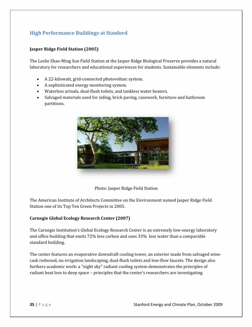
High Performance Buildings at Stanford
Jasper Ridge Field Station (2005)
The Leslie Shao‐Ming Sun Field Station at the Jasper Ridge Biological Preserve provides a natural laboratory for researchers and educational experiences for students. Sustainable elements include:
• A 22‐kilowatt, grid‐connected photovoltaic system. • A sophisticated energy monitoring system. • Waterless urinals, dual‐flush toilets, and tankless water heaters. • Salvaged materials used for siding, brick paving, casework, furniture and bathroom
partitions.
Photo: Jasper Ridge Field Station
The American Institute of Architects Committee on the Environment named Jasper Ridge Field Station one of its Top Ten Green Projects in 2005.
Carnegie Global Ecology Research Center (2007)
The Carnegie Institution’s Global Ecology Research Center is an extremely low‐energy laboratory and office building that emits 72% less carbon and uses 33% less water than a comparable standard building.
The center features an evaporative downdraft cooling tower, an exterior made from salvaged wine‐cask redwood, no‐irrigation landscaping, dual‐flush toilets and low‐flow faucets. The design also furthers academic work: a "night sky" radiant cooling system demonstrates the principles of radiant heat loss to deep space – principles that the center’s researchers are investigating.

36 | P a g e Stanford Energy and Climate Plan, October 2009
Photo: Carnegie Global Ecology Research Center
The American Institute of Architects Committee on the Environment named the Global Ecology Research Center one of its Top Ten Green Projects in 2007.
Science and Engineering Quad (2008 2012)
The Jerry Yang and Akiko Yamazaki Environment + Energy (Y2E2) Building is the first of four buildings to be completed between now and 2012 that will make up the Science and Engineering Quad (SEQ). SEQ describes 500,000 square feet of interdisciplinary teaching and research space within four highly‐sustainable buildings. The sustainability performance goals were specifically outlined in the Master Plan as the “SEQ Performance Criteria for Sustainable Buildings”. They are an extension of the Stanford’s existing Sustainable Design Guidelines, and were modeled and influenced by the LEEDLEED® NC and LABS21 rating systems.
Y2E2 in the Science & Engineering Quad Science & Engineering Quad

37 | P a g e Stanford Energy and Climate Plan, October 2009
The focus topic areas and corresponding performance achievements are as follows:
• Carbon: Achieve operational carbon neutrality • Energy: Reduced energy consumption cost by approximately 50% based on the national
energy code standards for a similar building type • Water: Reduced fixture potable water consumption by 90%. Reduce total water
consumption (including indirect water consumption for cooing) by 50%. • Indoor Environmental Quality: Day lighting of 78 ‐ 80% of above grade spaces. Providing
operable windows throughout all above grade perimeter spaces (full natural ventilation is provided on East and North exposures while mixed mode conditioning is provided on the South and West exposures)
• Economic: Under budget. “Sustainability Premium” of 1% ‐ 4.6% of construction budget. 7%‐ 33% return on investment for energy related systems.
• Learning: Ongoing measurement and verification of performance
The Y2E2 Building is a green design showcase. It provides a home for cross‐disciplinary research and teaching focused on sustainability and the building itself serves as a learning tool.
Photo: Y2E2 North East Exposure
The 166,500‐square‐foot building uses 56% less energy (per energy costs based on regulated energy comparison) than a traditional building of comparable size and 50% less total water than one with traditional fixtures and systems. Significant portions need no air conditioning and much of the building relies on natural light during the day. Features include:
• A high‐performance envelope (roof, walls, windows, sunshades, and light shelves) that reduces heating and cooling loads.
• Natural ventilation via internal atria, windows, and vents. • Three solar photovoltaic installations that offset energy use. • Water conservation systems, including waterless urinals and dual‐flush toilets; recycled
water from Stanford’s Central Energy Facility is used in toilets and for lab processes.

38 | P a g e Stanford Energy and Climate Plan, October 2009
• Extensive use of recycled materials and sustainable products, such as bamboo. Exposed concrete floors significantly reduce carpet use and saved tons of raw materials.
The Y2E2 building is the first of four buildings that will make up the Science and Engineering Quad 2. The remaining three buildings will be built to use 50% less energy than traditional buildings. San Francisco Business Times named Environment + Energy the Best Green Building in the Bay Area in March 2008.
Knight Management Center (2011)
Knight Management Center, the new home of Stanford’s Graduate School of Business, is striving to achieve a Leadership in Energy and Environmental Design (LEED) Platinum certification – the highest level offered by the U.S. Green Building Council’s rating program.
Slated to open in winter 2011, the center will comprise 360,000 square feet in multiple buildings. It is expected that the center will reduce total energy costs by 42% compared to similar traditional buildings and achieve all 10 possible points in the LEED Green Building Rating System. As much as 12% of the center’s energy may be supplied by on‐site photovoltaic panels.
The project will exceed the highest LEED standards for water conservation. Solar hot water collectors will provide domestic water and plans include harvesting rainwater on‐site and recycling water from the Central Energy Facility, both to be used for toilets and irrigation.
Photo: LEED Platinum GSB Complex – South West Corner
Sustainable features will also include natural ventilation, day lighting, and high‐performance active building systems. Other energy‐saving technologies may include under‐floor air distribution, displacement ventilation, and radiant cooling and heating. Some areas will need no air conditioning.

39 | P a g e Stanford Energy and Climate Plan, October 2009
The Green Dorm (2014)
This project, a collaboration between School of Engineering students, faculty, and Student Housing’s construction and design team, will be a living laboratory. Its energy, water, and structural systems will be continuously monitored, evaluated, and modified. When constructed, the dorm will incorporate the most advanced materials, architectural design practices, and energy and water technologies available. It is expected to generate more electricity than it uses and emit no net carbon, as well as use half the water of comparable dorms.
Photo: Green Dorm Plan, EHDD Architecture
Plans call for using solar panels and hydrogen fuel cells as the primary source of energy, reusing rainwater and gray water for irrigation, laundry and toilets, and other sustainable practices. The project is expected to be completed in 2014.

40 | P a g e Stanford Energy and Climate Plan, October 2009
Chapter 5: Reducing Energy Use in Existing Buildings While the University has pursued aggressive demand‐side energy management for many years, continued campus expansion calls for even greater attention to demand reduction and energy efficiency. Reducing energy use is central to creating a sustainable campus. It is also a formidable task, given the growing energy needs of research universities. Stanford has a strong foundation for success, however—Stanford is building on a decades‐long commitment to energy conservation and efficiency, as well as the advantages of a temperate climate and strong state energy codes. Current energy‐saving strategies will continually decrease consumption by existing buildings, but campus growth is likely to outpace those savings, requiring new efforts. Our recent experience illustrates why: total energy use increased 13% from 2000 to 2007, due to new construction, more energy‐intensive research and more people and electricity‐using equipment in existing buildings. Energy intensity (energy use per square foot) increased as well. By building on Stanford’s substantial successes and drawing on Stanford’s culture of innovation and leadership, the demand‐side energy management will continue to be a critical driver in reducing campus emissions. This chapter outlines the key initiatives and strategies for Stanford’s demand‐side energy management methodologies, especially as they relate to the Energy and Climate Plan.
Existing Energy Conservation Initiatives Energy Retrofit Program (ERP) The purpose of the Energy Retrofit Program (ERP) is to reduce overall energy costs on the Stanford University campus by improving the energy efficiency of building components, such as lighting, motors, and windows. Since 1993 over 300 ERP projects have been completed with an estimated energy avoidance of 240 million kWh. Because ERP projects are low risk, use technologies that are well understood, and have a positive return on investment, they should be considered an important part of Stanford’s GHG strategy. Whole Building Retrofit Program The Whole Building Retrofit Program is an effort to identify energy efficiency measures through comprehensive energy studies in Stanford’s largest buildings. The original study of twelve buildings identified $4 million of annual savings at a first cost of $15 million dollars. The next step is to complete implementation of the projects identified in the original study, while beginning study on

41 | P a g e Stanford Energy and Climate Plan, October 2009
the next group of buildings. In total, the program is expected to achieve almost $6 million of annual energy savings at a construction cost of roughly 27 million dollars. Energy Conservation Incentive Program (ECIP) Stanford University’s Energy Conservation Incentive Program (ECIP) is one example of a program designed to reduce energy use through human behavior rather than technology. The ECIP uses financial rewards and penalties to promote more efficient daily habits and purchasing decisions by Stanford’s schools and administrative units. This program helps reduce electricity use inexpensively and has achieved an overall 3% reduction thus far while also fostering a campus culture that supports energy efficiency activities on both personal and institutional levels. Building Operating Strategies Turning off building HVAC systems when they are not needed saves energy and reduces GHG emissions with minimal cost. Savings can also be achieved by establishing and implementing campus‐wide indoor temperature guidelines. All of these can be achieved with relatively simple software solutions and increased communication between organizations and control systems. Excessive Use Monitoring Excessive use monitoring can help identify and correct significant problems with building operation more quickly than might otherwise occur. A number of options for enhancing Stanford’s current excessive use monitoring are available, and the potential for reducing energy wasted in existing (and future) academic buildings appears to be significant – on the order of 15%. However, harvesting this potential will require both a modest up‐front investment and ongoing commitment of resources in both SEM and BGM to take the actions necessary to investigate and correct building operation problems identified through monitoring. Building HVAC Recommissioning Building HVAC Re‐Commissioning is a process to periodically review operation of building heating, ventilation, and air conditioning systems to insure they are performing at their optimum design efficiency. Significant energy savings from 1% to as much as 10%, particularly in steam and chilled water, are achievable from the process of “tuning up” existing systems without the need for any physical improvements to the building or its systems. In addition the process helps identify opportunities for physical upgrades to those buildings and systems that may be funded through the Energy Retrofit Program or other means.

42 | P a g e Stanford Energy and Climate Plan, October 2009
Building & Grounds Maintenance Fleet Over time, the University has accumulated a large number of gasoline burning vehicles for business conducted on and off campus. In preparing the data for the replacement plan, one can see it is common for departments to keep vehicles well beyond their amortization periods with some vehicles aged 20 years and more. These two factors combined have resulted in a fleet made up mostly of gasoline burning vehicles or vehicles that have been held long enough by many departments that their emissions standards are far below those required of vehicles manufactured in recent model years.
New Energy Conservation Initiatives Current energy‐saving strategies are expected to push energy consumption down through 2011, but by 2012 additional use from new buildings is likely to require further conservation efforts. The following new efforts are calculated into the Energy and Climate Plan. A. High Efficiency Transformers Low‐voltage transformers are used to convert the 480 Volt power delivered at the building entrance to the lower 120 Volt power supplied at the building’s electrical outlets. A typical building may have as many as half‐a‐dozen distribution transformers installed in various electrical rooms. Transformers lose power in the conversion process. The extent of these losses is a measure of a transformer’s efficiency. Efficiency increases can have a substantial impact on total building electrical consumption because transformers operate continuously whether outlets are being used or not. Furthermore, because transformers emit wasted electricity as heat, inefficient transformers place a higher burden on a building’s cooling system.
Photo: High Efficiency Transformers
Stanford recently entered a partnership with Powersmiths® that will lead to extensive use of higher efficiency power transformers for new construction and building renovations. The E‐Saver‐3 transformers meet the Department of Energy’s CSL‐3 standard, which offers the optimal life‐cycle balance between improved efficiency and additional cost. If only 75 standard low‐voltage transformers were upgraded to the CSL‐3 standard, the electrical savings per year would be approximately 450,000 kWh.

43 | P a g e Stanford Energy and Climate Plan, October 2009
B. Room Temperature Biological Sample Storage Stanford University has completed a pilot project to evaluate an innovative technology that promises to achieve sustainability goals by reducing laboratory energy consumption (along with associated costs and greenhouse gas emissions), optimize use of valuable lab space, and better protect priceless biological samples in the event of an earthquake or other disaster. Using a stabilization technology developed by Biomatrica®, biological samples such as DNA and RNA can be safely protected and stored at ambient (room) temperature as opposed to traditional storage in ultra‐cold freezer. The four‐month project engaged twelve research laboratories to assess the number of samples that could be moved from freezers to ambient temperature storage, validate the Biomatrica technology, actually transfer 70,000 samples from freezer storage to room temperature storage, and extrapolate the potential benefits to the entire Stanford University campus over ten years. Adoption of this technology for the existing sample collection alone offers potential to reduce the University’s annual electricity use by nearly two million kWh and chilled water consumption by over 300,000 ton‐hours (about 2% and 0.5% of the campus total, respectively), thereby avoiding more than 800 metric tons of carbon dioxide emissions. Such an investment in new sample storage technology could pay for itself within two years. Current: Freezing methodology; future: dry storage cabinet keeping the samples at a constant humidity, the new technology is in the wells of the plates and tubes, offering the advantage of a dense storage footprint.

44 | P a g e Stanford Energy and Climate Plan, October 2009
C. Sustainable Information Technology Initiatives Stanford University has a significant information technology infrastructure — faculty, staff, and students have approximately 35,000 computers on their desks and there are an estimated 6000 servers used for administrative and research computing across the university. When as much as 50% of the energy footprint of a server is the result of the cooling required to keep it running, factoring in facility savings is critical. Sustainable IT at Stanford is a joint effort between the Department of Sustainability and Energy Management and Information Technology Services, which enables the initiative to take a holistic look at our computing infrastructure, both the machines themselves and the buildings they are in. Specifically for IT, from choosing smart power supplies and enabling desktop power management, to redesigning data centers and server rooms, the upfront costs of these efforts have a short return on investment in energy savings alone. Also, Stanford’s leadership and leverage in IT innovation and implementation give the university an edge among peer institutions. Sustainable IT reaches out to faculty around campus to identify research focused on computing energy efficiency, and bring together staff and faculty to help further these efforts. Desktop Computers and Office Equipment
• Desktop Computer Power Management — In 2007, Stanford deployed a centrally‐controlled
Desktop Power Management tool to help set, and track, power management settings provided by the Windows and Macintosh operating systems. Desktop Power Management is enabled on over 9000 computers across the university.
• Energysaving Power Strips — In addition to turning off computers and monitors, Stanford is
working to reduce ‘phantom’ power. When computing peripherals are in standby mode, they continue to draw meaningful amounts of electricity, yet are producing no useful work. By deploying Smart Powerstrips, Stanford is able to automatically turn peripherals off when computers go off thus reducing our energy usage.
• Hardware Procurement — Stanford has joined the Climate Savers Computing Initiative, and
we are working with Procurement to ensure we purchase energy efficient servers whenever possible. Used equipment can be found on the Stanford Reuse site, where equipment in good condition is offered to others around campus.

45 | P a g e Stanford Energy and Climate Plan, October 2009
Data Centers • Data Center Energy Efficiency — The campus data center is one of the largest energy‐using
buildings on campus. Stanford has developed an overall plan to reduce energy usage by modifying the computing infrastructure, the facility, and the infrastructure components. Specific efforts that are being implemented in Stanford campus datacenters include revamping the cooling system, restructuring the racks, replacing lighting, enclosing aisles, adding sensors and enabling more refined monitoring.
• Scientific Research Computing Facility — Research Computing is high intensity computing
used by our faculty for their research projects and is one of the fastest growing users of energy on campus. We have designs for a new Research Computing Facility that will massively reduce the cooling needed to keep these high‐intensity servers running. Once we have highly efficient data centers, we plan to work with schools and departments across the university to ensure their servers are located in the most energy efficient locations.
• Server Replacement, Consolidation, and Virtualization — One of the most effective ways to
reduce energy in the data center is to reduce the number of computers it takes to produce the same output. Replacing old hardware with new, more energy efficient hardware, consolidating under‐utilized servers, and deploying server virtualization are all means to achieve this goal.
• Centralized Data Storage — Data that is stored in a central directory, rather than in local
devices, saves energy by allowing the university to manage storage capacity more effectively and more energy efficiently.
Energy Saving Work Practices • Work Anywhere IT Infrastructure can be used to enable work practices that save energy. The
university is actively pursuing a ‘work anywhere’ philosophy, and provides free online conferencing, telepresence conference rooms, thin clients, and remote offices which reduce employee driving and commuting.

46 | P a g e Stanford Energy and Climate Plan, October 2009
Energy Conservation from Individual Behavior (in pilot) Stanford will continue to build on a strong foundation for energy conservation, as the energy intensity for new construction and major renovations often continue to increase. The source of these solutions will continue to be a combination of effective deployment of innovative technology, as well as a noticeable and measureable shift in user behavior towards energy conservation. The sustainability program initiatives indicate that there is great potential in harnessing the conservation benefits from individual action. Not only is this a personally significant contribution for campus population, there is a desire to quantitatively express the value of these individual actions, coordinated through department or school level efforts. Sustainability programs are moving towards establishing department‐level contacts, helping form school‐level sustainability committees, identifying specific evaluation criteria and standards, and training committee members on key actions that can help conserve natural resources.
Photo: President Hennessey on a tour of the Jasper Ridge Biological Preserve
In early 2009, Stanford has started key pilot projects to quantify the costs and benefits of individual action, with an end goal of creating a business case for implementing these actions for the whole campus. One pilot project, for example, through a combination of desktop power management, smart power strips, timers, and decommissioning unnecessary equipment and excess lighting, has seen its electricity consumption drop by nearly 20%. Though the analysis on behavioral projects is not a part of the infrastructure focus Climate and Energy Plan, in coming years we anticipate well identified and implementable projects to join the portfolio offered in this blueprint.

47 | P a g e Stanford Energy and Climate Plan, October 2009
Chapter 6: Energy Supply Options
Along with strong new building energy efficiency standards to reduce the impacts of growth (discussed in Chapter 4), and adept conservation measures to reduce energy use in existing facilities (discussed in Chapter 5), an innovative energy supply is the third key strategy of this Energy and Climate Plan. This chapter describes the different long term energy supply options considered by Stanford, provides an analysis of the costs and greenhouse gas emissions for meeting campus energy needs under each option, and presents key findings regarding energy supply for a long term horizon through 2050.
Energy Supply Options The following energy supply options were considered for Stanford: Business As Usual (BAU): a third party owned and operated on‐site cogeneration plant
Combined Heat & Power (CHP): a new Stanford owned and operated on‐site cogeneration plant;
Separate Heat & Power (SHP): a new Stanford owned and operated gas boilers and electric chillers plant with imported electricity;
Regeneration Heat Recovery (HR): a variation of SHP involving significant heat recovery at the central energy facility but which requires conversion of the campus steam distribution system to hot water.
The cost of significant direct emissions reductions under the CHP, SHP, and Regeneration options could be substantial, compelling consideration of the use of carbon instruments that might indirectly achieve comparable emission reductions. To do this the different options are all tested with the use of carbon instruments at several prices and the results are presented in this chapter. However detailed findings about the viability of carbon instruments (discussed in Chapter 8) indicates significant economic, regulatory, and environmental risk in considering their use for any significant role in the planning of a long term energy supply.

48 | P a g e Stanford Energy and Climate Plan, October 2009
BusinessAsUsual (BAU) In the BAU option (Figure 6‐1) a third party owns and operates an on‐campus natural gas fueled cogeneration plant for the dual purposes of selling electricity to the grid and selling electricity and thermal energy to the campus. Because sales of power to the grid generates more waste heat than is actually needed by the campus for heating and hot water this excess heat is used for steam powered chilled water production.
Figure 61 Business As Usual CHP
Grid interconnection for
power sales and backupCogeneration
Unit
Power for Lighting and Equipment
Steam for Building
Heating and Hot Water
Heat Recovery
Steam Generator
Heat
Fossil Fuel Electricity
Electric and
Steam Chillers
Unwanted Heat to
Atmosphere
Condensate Return
Steam Supply
Cooling Tower
Electricity
Water
Chilled Water for Cooling Buildings
Ice Storage
Chilled Water
From Cogen Unit
Solar, air, lighting,
equipment, and human heat into buildings
Steam
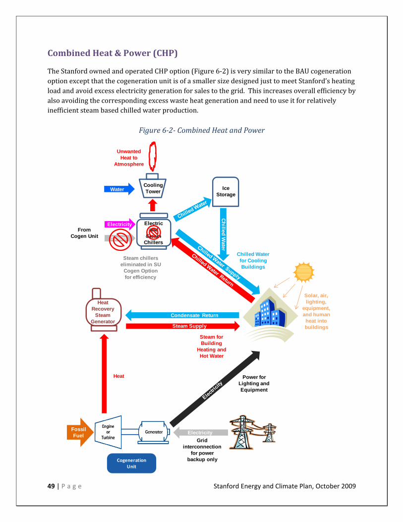
49 | P a g e Stanford Energy and Climate Plan, October 2009
Combined Heat & Power (CHP) The Stanford owned and operated CHP option (Figure 6‐2) is very similar to the BAU cogeneration option except that the cogeneration unit is of a smaller size designed just to meet Stanford’s heating load and avoid excess electricity generation for sales to the grid. This increases overall efficiency by also avoiding the corresponding excess waste heat generation and need to use it for relatively inefficient steam based chilled water production.
Figure 62 Combined Heat and Power
Cogeneration Unit
Power for Lighting and Equipment
Steam for Building
Heating and Hot Water
Heat Recovery
Steam Generator
Heat
Fossil Fuel Electricity
Grid interconnection
for power backup only
Unwanted Heat to
Atmosphere
Condensate Return
Steam Supply
Cooling TowerWater
Chilled Water for Cooling Buildings
Ice Storage
Chilled Water
Solar, air, lighting,
equipment, and human heat into buildings
Electric and
Steam Chillers
ElectricityFrom
Cogen Unit Steam
Steam chillers eliminated in SU
Cogen Option for efficiency

50 | P a g e Stanford Energy and Climate Plan, October 2009
Separate Heat & Power (SHP) With a Separate Heat and Power option (Figure 6‐3) electricity and heat energy for Stanford could be produced separately. The electricity can be generated on‐site or off‐site with either fossil fuel or renewable energy sources. Heat can be produced with either fossil fuel or electric boilers, or with on‐site solar thermal equipment. Chilled water is produced with efficient electric powered chillers.
Figure 63 Separate Heat and Power
Chiller
Unwanted Heat to
Atmosphere
Condensate Return
Steam Supply
Cooling Tower
Electricity
Solar, air, lighting,
equipment, and human heat into buildings
Water
Steam Boiler
Fossil Fuel
Chilled Water for Cooling Buildings
Steam for Building
Heating and Hot Water
Ice Storage
Chilled Water
From Grid or On-site
Renewables
Power for Lighting
and Equipment
Imported Fossil Fueled Generation
Imported Renewable Generation
and/or
100% Fossil Fuel
Heat
Fossil Fuel
PotentialOn-campus
Solar Thermal
and/or
PotentialOn-
campusSolar
Electricity

51 | P a g e Stanford Energy and Climate Plan, October 2009
Regeneration Regeneration (Figure 6‐4) is the use of SHP with recovery and reuse of heat normally discarded into the atmosphere via cooling towers in the chilled water system. It differs from Cogeneration in that it productively uses waste heat supplied by the environment (mostly direct and indirect solar heating of buildings) rather than waste heat supplied by the combustion of fossil fuel.
Figure 64 Regeneration Scheme
Recovered Heat to
Productive Use
Electricity
Hot Water Boiler
Unwanted Heat to
Atmosphere
Cooling TowerWater
50% Recovered
Heat
Hot Water Supply
Hot Water Return
Hot
Wat
er R
etur
n
Hot W
ater
Sup
ply
Electric Chillers
Heat Recovery Chillers
From Grid or On-site
Renewables
Solar, air, lighting,
equipment, and human heat into buildings
Chilled Water for Cooling Buildings
Ice Storage
Chilled W
ater
Power for Lighting
and Equipment
PotentialOn-
campusSolar
ElectricityImported Fossil
Fueled Generation
Imported Renewable Generation
and/or
Fossil Fuel
Fossil Fuel
50% Fossil Fuel Heat
PotentialOn-campus
Solar Thermal
and/or
Hot Water for Building
Heating and Hot Water

52 | P a g e Stanford Energy and Climate Plan, October 2009
Regeneration Potential at Stanford
Regeneration has potential application at any location where cooling systems collect and discard heat from buildings or processes at the same time low grade heat (<175F) is produced for heating, hot water, or other applications. Anytime there is a real time overlap in the two processes or availability of hot thermal storage there is an opportunity to use the heat collected by the cooling process to meet the energy needs of the low grade heating processes instead of burning fossil fuel. This overlap will vary by the nature of facilities and the climate where they are located however productive use of any overlap may be one of the larger potential tools in energy conservation and GHG reduction. At Stanford analysis of a full year of hourly heat and chilled water production data at the Central Energy Facility (CEF) revealed a real time 70% overlap in btu collected by the chilled water system and discarded out cooling towers versus btu generated by fossil fuel and delivered to buildings via the steam distribution system. This can be seen as the shaded areas on the charts on the following page, and more details about this overlap analysis are provided in Appendix F. Further analysis revealed than if a one day volume of hot thermal storage could be devised another 10%, or 80% total of the btu collected by the chilled water system could be put to productive use for heating needs. Adding in chiller machine heat energy that is also normally discarded it was determined that about 50% of the total annual campus heating load could be met with recovered heat, supplanting a significant amount of fossil fuel use and associated energy cost and GHG emissions. In addition to building heating and hot water production, if other productive uses of this recovered heat can be found the collective reduction of cost and GHG emissions from heat recovery is even greater. Also, if ground source heat pumping in winter or other means to collect heat occurring freely from the environment can be devised using the heat recovery system additional substantial reductions in fossil fuel and associated cost and GHG reduction use may be possible. Furthermore, because wet cooling towers are currently used for discharging heat from the cooling process to the atmosphere a significant amount of water can be saved through heat recovery. It is estimated that about 22% of the total campus domestic fresh water supply is consumed by the CEF cooling towers. Using heat recovery for 70% to 80% of the chilled water flow as mentioned above will provide a corresponding reduction in CEF water use, thus reducing overall campus water use by about 15%. Though a heat recovery system would require more electricity than a standard chilled water system, the benefit of the heat recovered would be much greater than the impact of the added electricity in both cost and GHG emissions. Furthermore, the potential for meeting this and other electricity loads with renewable energy under an SHP or Regeneration scheme is a desirable flexibility that could allow further GHG reductions via a shift away from the use of fossil fuel.

53 | P a g e Stanford Energy and Climate Plan, October 2009
Summer
Spring /Fall
Winter
Figure 65 Heat Recovery
Potential
0102030405060708090
100110120130140150160170180190200210
MMbtu
Hour of Day
Stanford UniversityHeat Recovery Potential at Central Energy Facility
Sample Date 7/23/2008
Heating
Cooling
Thermal Overlap
0102030405060708090
100110120130140150160170180190200210
MMbtu
Hour of Day
Stanford UniversityHeat Recovery Potential at Central Energy Facility
Sample Date 4/16/2008
Heating
Cooling
Thermal Overlap
0102030405060708090
100110120130140150160170180190200210
MMbtu
Hour of Day
Stanford UniversityHeat Recovery Potential at Central Energy Facility
Sample Date 1/23/2008
Heating
Cooling
Thermal Overlap

54 | P a g e Stanford Energy and Climate Plan, October 2009
Compatibility Considerations with CHP and SHP Because the CHP process would burn fossil fuel to make electricity and use the waste heat to meet campus heating demands, CHP is essentially incompatible with processes that would supply heat by other means, such as heat recovery or direct production of heat via renewable sources such as solar steam generators, geosource heat pumps, and so forth. The cogeneration option is physically incompatible with any significant heat recovery or alternative heat production schemes; hence there is no CHP + Heat Recovery option possible or analyzed herein. SHP on the other hand is fully compatible with heat recovery and alternative forms of heat production. In SHP, heat production is not dependent upon nor tied to electricity generation and instead heat is generated by separate steam or hot water boilers. Operation of these individual pieces of equipment can be tailored to compliment other forms of heat production, allowing maximum use of lower cost, cleaner heat than that generated by fossil fuel via CHP. Converting to a Hot Water Distribution System In considering the potential for heat recovery at this scale, a complete conversion of the campus steam distribution system to a hot water distribution system would be required. Though this represents a significant operational challenge other universities and cities are already in the process or considering such a change based solely on the merits of lower long term operation and maintenance cost without even considering heat recovery as an enabling requirement. As explained later in this chapter the estimated cost of such a change is also substantial at over $100 million, however the investment is recouped in a number of ways including:
• heating system line losses could be reduced from about 12% to 4% with the conversion; • operation and maintenance cost would be much lower with a hot water system; • substantial capital costs for replacement of aging portions of the steam system could be
avoided through a conversion; and • capital costs for future system expansion and interconnection to new buildings would be
much cheaper with hot water. A discussion of the benefits of converting the steam distribution system to hot water, along with case histories of similar applications and a conceptual phasing plan are included in Appendix G.

55 | P a g e Stanford Energy and Climate Plan, October 2009
Model Variables Energy Use Data The initial GHG Reduction Options report in 2008 benefitted from a wealth of accurate data on overall energy production and use at the university for at least ten years. To facilitate even more in‐depth investigation of options, detailed information on energy flows in and out of the Central Energy Facility on an hourly and daily basis rather than monthly or annually was needed. A complete dataset of steam and chilled water production figures for the CEF for every hour of every day for a one year period was prepared and used to assess the potential for heat recovery and other analysis. A copy of one day from the dataset is provided in Appendix H.
Projections of Campus Growth As discussed in Chapter 3, forecasting long term energy demands required consideration of two factors growth in campus size (in terms of GSF) and increases in the average energy intensity (in terms of kWh/GSF) of the buildings. Analysis confirmed that the average energy use in Stanford buildings was steadily growing due to increases in research laboratories and increased building ‘plug’ loads, including research and administrative computing and cold storage of biological and medical specimens. Using these updated energy intensity factors, current near term building plans, and three long range growth scenarios provided by university planners (minimal, moderate, and aggressive) energy demand projections for each of the three campus growth scenarios were prepared and used for analyzing supply options. Copies are provided in Appendix E. Variables and Assumptions A critical component of the analysis is the set of assumptions and variables used for future natural gas, market electricity, investor owned utility (IOU), and renewable electricity prices and carbon content. Also important are a number of other variables such as future load projections and equipment efficiencies for cogeneration units, boilers, and combined cycle gas turbine (CCGT) generating stations. To arrive at the variables for the model the team reviewed data from Stanford central energy facility operations; current reports from the California Energy Commission and other state agencies; the DOE Energy Information Administration, EPA, and other federal agencies; state utility companies including PG&E; consultant reports; and numerous other sources which are cited throughout this report.
Appendix I provides a list and discussion of the variables and assumptions used in the energy supply analysis. A summary of some of the key variables is provided below.

56 | P a g e Stanford Energy and Climate Plan, October 2009
Summary: Variables and Performance Factors Used in Energy and Climate Plan Modeling 1. Campus Growth Minimal (115,000 sf/year)
Moderate (200,000 sf/year) Aggressive (300,000 sf/year)
2. Natural Gas cost $6.50 to $13.16 per MMbtu
3. Renewable Electricity cost $90 to $140 per MWh
4. GHG Emission Reduction from 2000 Baseline No GHG restrictions to 100%
5. Heat Recovery 50% to 70%
6. Distribution System Losses High Voltage (Imported supply) 2.3% High Voltage (On‐site Cogen supply) 2.8%
Steam (Supply & Return) 12% Hot Water (Supply & Return) 4% Chilled Water (Supply & Return) 2%
7. Market Electricity cost $88 to $105 per MWh
8. Average Carbon Content of California Grid Electricity 493 lb/MWh lowering to 357 lb/MWh
9. Investor Owned Utility Electricity cost $88 to $105 per MWh
10. Average Carbon Content of PG&E Electricity 493 lb/MWh lowering to 357 lb/MWh
11. Grid Gas Turbine Combined Cycle Efficiency 40% to 60%
12. New Stanford Cogeneration Plant Efficiency 69%
13. Gas Boiler Efficiency 85%
14. Electric Chilled Water Production Efficiency .55 kwh/ton‐hour
15. Heat Recovery Chiller Coefficients of Performance COPR 2.62, COPH 3.68 16. Carbon Instruments Unit Cost $25/$50 per m‐ton Note: A scenario (within variable number 4 above) significantly different than all the others is the ‘No GHG Limits’ scenario, which needs to be interpreted in its proper context. Under this scenario, it is assumed that no GHG limitations are imposed on Stanford. It may choose to provide its energy in the most economical way without a restriction in GHG emissions growth above year 2000 levels or associated cost impacts such as from carbon taxes on fuel or abating emissions through a regulated cap and trade program. Given known regulatory actions to date this scenario is unlikely but still possible at this time and so has been included for comparative purposes, with special notation in discussions where it is covered.

57 | P a g e Stanford Energy and Climate Plan, October 2009
Capital Cost Detailed capital schedules and cost estimates for energy system expansion, conversion, and renewal from 2010 to 2050 were prepared for each option and are provided in Appendix Q. The estimated total capital costs for each option over this period, including all overheads and project management fees, are:
Business‐As‐Usual $520 million CHP $570 million SHP $503 million Heat Recovery $589 million
All options include an estimated $130 million in potential facility improvement fees to PG&E for off‐site high voltage system renewal and expansion to support campus long term growth. These fees are not well vetted but are conservatively included so as not to underestimate long term capital costs for campus energy supply. The main differences in cost between the options are as follows: BAU • Does not include $50 million for the replacement cogeneration unit included in the CHP total SHP • Does not include the $50 million replacement cogeneration unit • Reuses CEF Cogen space for future chillers and avoids the cost of a new east campus chiller
building • Reuses Cogen cooling tower to reduce total new cooling tower costs • Includes an additional backup steam boiler for redundancy not required in BAU and CHP
options Heat Recovery • Same as SHP but with less steam boilers due to use of heat recovery chillers for producing heat • Includes $107 million to convert the steam distribution system to hot water plus $21 million for
associated changes to building systems; • Includes much lower long term capital renewal cost for hot water system than steam system
renewal cost included in all other options These costs are included in the form of annual debt service costs in the total cost for each of the options discussed later in this chapter. In all instances where capital costs are shown for information in addition to total option costs on comparison charts, the total cost includes capital debt service. Parallel Energy Models Due to the magnitude and complexity of the energy supply issue, two parallel and complementary long range energy models were developed for the analysis by different SEM engineering staff to take advantage of available in‐house expertise and institutional knowledge. The two models were periodically calibrated and reconciled to assure reliable results for decision making. Illustrations of

58 | P a g e Stanford Energy and Climate Plan, October 2009
the two energy models are provided in Appendix J, though due to their complexity, detailed information on their construction and use are not included.
Additional Peer Review
After completion of advanced modeling and analysis, a third‐party peer review was commissioned to check the results and determine if any other major options for long term energy supply should have been considered. Because of the significance of the findings and complexity of the analysis, two separate consultants as well as faculty and staff with specialized expertise were engaged for the peer review. The review also sought advice on converting the campus steam distribution system to a hot water system. The peer review findings are in Appendix O, but the key recommendations were:
1. Conservatively assume that over time deregulation of the California electricity market does not result in significant differences in the relative cost and carbon content of market and investor owned utility electricity. This will also provide a hedge against the possibility that Direct Access is not reopened and the university would only be able to procure power from PG&E;
2. Increase the estimated cost of converting the campus steam distribution system to hot water from $80 million to $107 million;
3. Increase the assumed annual non‐fuel O&M costs for an on‐campus cogeneration plant from $7.20 per MWh to $15.00 per MWh;
4. Reduce assumed future gas boiler efficiency from 90% to 85%;
5. Increase assumed electric chiller efficiency from .65 kW/ton to .55 kW/ton;
6. Increase the resolution of the energy model by applying assumptions and variables to individual annual projected loads and summing the individual years results rather than using a net long term average, despite the linear nature of the long term load projections;

59 | P a g e Stanford Energy and Climate Plan, October 2009
7. Assume very strong regulation of GHG beginning as early as 2012 and build in the influence of this climate change regulation into the base case of the energy model;
8. Pursue a lower temperature design for the hot water system to maximize energy efficiency and design margin of safety;
9. Consider directly interconnecting building industrial hot water loops to the main campus hot water distribution system to reduce cost and improve operational quality control of building hot water systems.
These key findings and recommendations were incorporated into the final energy supply analysis and conclusions, which were then further reviewed with campus advisory teams and senior management before incorporation into this Energy and Climate Action Plan.
Model Analysis Stanford’s Energy and Climate Plan effort invested substantial time and resources to take a fresh look at holistic long term energy supply options and the university’s existing Central Energy Facility (CEF). This included an investigation into the potential impacts to the regional electricity grid and statewide GHG reduction strategies (AB32) if cogeneration were eliminated at Stanford. A key goal of this analysis was to determine the most efficient and cost effective option for meeting Stanford’s electricity and thermal loads using Life Cycle Cost Analysis, while also considering relative cash flows and years to payback of higher capital investment options. The analysis also had to evaluate the flexibility (or lack thereof) the options would respectively provide for implementing future technologies that might allow further reduction in cost and GHG emissions at Stanford. The analysis considered, among other things: • Comparative Efficiency: This comparison was performed to address the question of whether
retaining cogeneration at Stanford would assist in statewide strategies for GHG reduction under AB32. Considering natural gas as the only likely permissible fossil fuel source and applying best available energy production technologies a comparison of overall fuel efficiency between the options was made over a reasonable sensitivity range. This was used to determine if any particular technology was clearly more efficient and would therefore result in fewer GHG emissions per unit of energy delivered.
• Comparative Total Cost, GHG Emissions, and Risk: This comparison considers the total life
cycle cost; initial capital outlay and debt service cash flow; economic risk and reaction to changes in gas and electricity costs; and options and costs for varying levels of GHG emissions reduction.

60 | P a g e Stanford Energy and Climate Plan, October 2009
Comparative Efficiency This comparison addresses the relative efficiency of the options and the question of whether or not continuing the use of CHP at Stanford will support statewide GHG reduction strategies that seek the most efficient overall forms of electricity and thermal production where fossil fuels are used. It should be noted that unlike the BAU and CHP options that must use 100% natural gas fuel, under the SHP and Regeneration options electricity may be supplied not only by a gas fired power plant but also by on‐campus or off‐campus renewable power, nuclear power, or other power mixes of varying efficiency and associated GHG emissions. For this reason this comparative efficiency test should not be considered an enabling test of the merits of CHP regarding both GHG emissions and economics, but rather only the first test it must pass in a thorough examination of cogeneration versus SHP and Regeneration alternatives. Figure 6‐6 shows the relative overall efficiencies of the BAU, CHP, SHP, and Regeneration options using the High Heating Value (HHV) of natural gas fuel and currently available technologies for meeting Stanford’s energy demands, including: • BAU: Current Cardinal Cogeneration Plant at 59% efficiency; • CHP: New cogeneration plant @ 69% efficiency; • SHP: Electricity from a range of combined cycle gas turbine plants (CCGT) of varying efficiencies
and heat from a gas fired steam boiler at 85% efficiency; • Regeneration: SHP plus Heat Recovery Chillers with a Coefficient of Performance of 5.44. Since the efficiency of the grid CCGT plant supplying power to Stanford under an SHP or Regeneration option may not be under its control the diagram provides a range from existing low efficiency plants at 38% to new state‐of‐the‐art plants up to 60%. In today’s terms the expected efficiency will likely range from a low side mix of existing baseload and peaking gas plants of 39% to a new baseload plant of 54% efficiency, with this range denoted by the two vertical dotted lines. Figure 6.6 shows that the overall efficiency of the SHP and Regeneration options is very dependent on the efficiency of the CCGT plant when considering the use of natural gas fuel only. That said, within the expected efficiency range the SHP option appears marginally better than the 59% efficient BAU option but clearly lower than the 69% efficient new Stanford owned and operated cogeneration option. Likewise the Regeneration option appears clearly superior to all other options across the expected range of CCGT power plant efficiencies. Comparative efficiencies of greater than 100% are possible for Regeneration due to the use of heat freely occurring in the environment that allows a total energy yield greater than the energy value of natural gas input. Figures 6‐7 and 6‐8 provide a more detailed explanation of the overall comparative efficiency of the CHP and Regeneration options at unit scale of one therm of gas input to cogeneration for Stanford’s electric and thermal load balance. The BAU and SHP options are omitted as they are clearly inferior to their more efficient new CHP and Regeneration counterparts across all CCGT efficiency ranges.

61 | P a g e Stanford Energy and Climate Plan, October 2009
Figure 66: Overall Comparative CHP, SHP, and Regeneration Efficiency
0%
20%
40%
60%
80%
100%
120%
38% 40% 42% 44% 46% 48% 50% 52% 54% 56% 58% 60%
Overall Co
mbine
d Efficiency (using
100% gas)
Efficiency of Gas Fired Combined Cycle Power Plant Providing Electricity for SHP Option
CHP w 69% Efficient Cogeneration
CHP w 59% Efficient Cogeneration
Range of expected grid power plant efficiencies
Figure 6‐7 Figure 6‐8

62 | P a g e Stanford Energy and Climate Plan, October 2009
Figure 6-7: CHP v Regeneration Efficiency w 39% CCGT Power
Cogeneration
Regeneration with 39% Efficient Power Plant (3% worse than Cogeneration)

63 | P a g e Stanford Energy and Climate Plan, October 2009
Figure 6-8: CHP v Regeneration Efficiency w 54% CCGT Power
Cogeneration
Regeneration with 54% Efficient Power Plant (24% better than Cogeneration)

64 | P a g e Stanford Energy and Climate Plan, October 2009
This analysis shows further that given the widespread availability of 85% efficient boilers across most load ranges the expected efficiency of a cogeneration unit must be about 12% to 15% greater than the expected efficiency of the CCGT unit that would supply electricity under an SHP option to make CHP more efficient. For example, as shown on Figure 6‐6 an 85% boiler and 57% gas plant is equivalent to a 69% cogeneration plant, a difference of 12% as shown by the intersection of the lines for those respective options. An 85% boiler and 44% gas plant is equivalent to a 59% cogeneration plant, a difference of 15%. This finding is consistent with European Union findings and regulations regarding designation of cogeneration units as ‘high efficiency’ as outlined in paragraph (11) of the DIRECTIVE 2004/8/EC OF THE EUROPEAN PARLIAMENT AND OF THE COUNCIL which states: “(11) High efficiency cogeneration is in this Directive defined by the energy savings obtained by combined production instead of separate production of heat and electricity. Energy savings of more than 10 % qualify for the term ‘highefficiency cogeneration’. To maximise the energy savings and to avoid energy savings being lost, the greatest attention must be paid to the functioning conditions of cogeneration units.” As noted earlier, the Regeneration heat recovery option is always more efficient than SHP alone and is significantly more efficient than CHP across most of the range of gas plant efficiencies possible. Also, with Regeneration overall efficiencies of more than 100% are possible as shown due to the use of heat freely occurring in the environment. The crossover point between Regeneration and CHP efficiency is when gas power plant efficiency is within about 28% of cogeneration plant efficiency. Currently, state of the art gas plant efficiency is within about 15% of state of the art cogeneration plant efficiencies at this scale, so Regeneration using 100% natural gas should be significantly more efficient than CHP for the foreseeable future. Given this analysis retaining cogeneration at Stanford is neither more efficient nor would it generate less GHG emissions than the Regeneration alternative. Therefore retaining cogeneration would not support statewide GHG reduction strategies under AB32 even though that legislation promotes the expansion of CHP in the state, presumably only at locations where it is more efficient than other alternatives. It is also noted that the SHP and Regeneration options offer fuel flexibility that CHP does not. Therefore, a comparison of efficiencies based only on natural gas should not be considered an enabling test for CHP but rather only the first test it must pass in an objective comparison with Regeneration and SHP for a particular site. Once best available technology for each type of equipment is determined for a given set of energy loads comparison of overall efficiencies and GHG emissions can and should be determined for different options. Also, beyond the selection of fuel sources other variables that must be tested to achieve a true long term comparison of options include future load growth, ranges of potential GHG emissions limits, fuel prices, capital and O&M costs. These considerations are explored in the following sections.

65 | P a g e Stanford Energy and Climate Plan, October 2009
Comparing Cost, GHG Emissions, and Risk To provide broad coverage of the potential cost outcomes for the different options both Net Present Value (NPV) and Cash Flow cost analyses were performed across sensitivity ranges for the most influential and least predictable major variables of: a) campus growth and b) gas‐to‐renewable electricity price ratio. Three campus growth rate projections (minimal, moderate, and aggressive) were selected to match scenarios considered in the campus Sustainable Development Study (SDS). Three gas‐to‐renewable electricity price ratios (high, medium, low) were selected to provide a plus or minus 20% price sensitivity range, yielding a total of nine modeling scenarios for the sensitivity analysis. See Figure 6‐9 below.
Figure 69: Variables Bins Used for Energy and Climate Action Modeling
Because variation in the assumed campus growth rate was determined to typically only affect the absolute size of the figures and not the relative differences between the options, only the results across the three energy price bins for the moderate campus growth scenario are shown in each section below. The model results for the other six bins (minimal and aggressive growth scenarios each across the three energy price ratios) are provided in the Appendix N for further reference. In addition to the sensitivity ranges to cover the potential impacts of key variables, three potential business strategies were modeled to provide flexibility in decision making:
Minimal Growth Scenario (115,000 sf/year)
Moderate Growth Scenario (200,000 sf/year)
Aggressive Growth Scenario (300,000 sf/year)
High Gas/Renewable
Electricity Cost Ratio
minimal growth, high ratio
moderate growth, high ratio
high growth, high ratio
Medium Gas/Renewable
Electricity Cost Ratio
minimal growth, medium ratio
moderate growth, medium ratio
high growth, medium ratio
Low Gas/Renewable
Electricity Cost Ratio
minimal growth, low ratio
moderate growth, low ratio
high growth, low ratio

66 | P a g e Stanford Energy and Climate Plan, October 2009
1. Cost only comparison of supply options without emissions limitations.
2. Cost comparison of supply options with direct emissions reduction.
3. Cost comparison of supply options with indirect emissions reduction via carbon instruments.
Net Present Value Analysis
1. NPV cost comparison of supply options without emissions limitations
The first potential business scenario examined is one where Stanford does not voluntarily and is not compelled to limit its GHG emissions. Figures 6‐10, 6‐11, and 6‐12 show the estimated net present value (NPV) cost for the Business‐As‐Usual (BAU), CHP, SHP and Heat Recovery (HR) options for this scenario which is labeled ‘No GHG Limits’. Other scenarios of varying GHG emissions reductions below year 2000 baseline are also shown on these charts and discussed in the next sections. These tree figures present costs for a moderate growth scenario from 2010 to 2050 at medium forecasted natural gas prices with a sensitivity range of plus or minus 20% (high and low gas‐to‐renewable electricity price ratios respectively).
Because carbon emissions are not monetized under the ‘No GHG Limits’ scenario the cost comparison of energy supply options under this scenario is highly dependent on assumptions about the quality (carbon content per unit of electricity) and cost of electricity purchased under the SHP and Heat Recovery options. This study conservatively assumes that Stanford is limited to purchasing only Investor Owned Utility power, which by regulatory mandate has fewer carbon emissions and a higher cost than other forms of available market power. This favors cogeneration because a monetary penalty is not applied for the much higher GHG emissions it emits, however it should be noted that other forms of power may soon be available to Stanford that would level the economic playing field for this scenario if efforts to reopen Direct Access in California now underway are successful. For these reasons and to provide a balanced context in the absence of monetizing GHG emissions, the relative emissions for each energy supply option under the ‘No GHG Limits’ scenario are called out via inset ‘bar and bubble’ charts that contrast for each option the relative NPV (colored bars) and embedded capital costs (red lines within the bars) on the left Y axis to the annual GHG emissions in 2050 (orange bubbles) and 2000 GHG levels (solid orange line) on the right Y axis.
The analysis shows that without monetizing GHG emissions, at medium and low gas‐to‐renewable price ratios CHP would be about 3% cheaper than Heat Recovery, although it would result in about two and a half times more GHG emissions by 2050. At high gas price ratios it would be about 5% more expensive and generate about ten times more GHG emissions because at those gas prices renewable energy, if procured on a long term basis through equity position or purchase power agreement, would cost less than market power with a gas component. For more information on how gas and market electricity price escalation interactions were modeled please see Appendix I.
In summary, if GHG emissions were not limited either voluntarily or through regulation, and if emissions are not monetized through carbon taxes or cap and trade mechanisms, CHP may offer

67 | P a g e Stanford Energy and Climate Plan, October 2009
slightly lower long term costs under the medium and low gas price scenarios but with significantly higher GHG emissions than university 2000 baseline levels. In the high gas price scenario Heat Recovery offers a modestly lower cost along with the substantial GHG emissions reduction as renewable electricity becomes a better value than market power with a significant fossil fuel component.
With those same notes on carbon monetization, SHP would cost from 6% to 12% more than CHP depending on gas price ratios but would offer 30% to 60% fewer GHG emissions than CHP.
2. NPV cost comparison of supply options with direct emissions reduction With CHP, greenhouse gas emissions from energy supply can only be reduced by decreasing the amount of natural gas consumed in the cogeneration plant for the production of electricity, heat, and chilled water. The more GHG Stanford would want to reduce the more the use of natural gas must be curtailed and replaced by renewable energy. This cardinal fact for Stanford’s climate action, especially with all the early emissions reduction actions that are already in place, is a strong motivator for the extensive analysis of energy supply options for this campus. What could be the most effective methods for phasing out natural gas use and phasing in renewable energy over time under CHP? The answer depends on the amount of emissions reduced and there is a threshold point that reveals the relative efficiency of the CHP and SHP energy supply options. The most effective way to decrease overall natural gas use in a CHP application is to divert some fuel from the cogeneration unit to backup steam boilers to satisfy heat demands in order to defer phasing‐in the use of electric boilers until absolutely necessary due to economic costs. This phase shift from cogeneration to boiler use for heating becomes complete at about a 40% emissions reduction target (below base level 2000), based on the relative equipment efficiencies and GHG factors used in this analysis. At this point a de facto SHP configuration results because the cogeneration unit is completely shut down and all heat is supplied by gas boilers and all electricity by imported power as shown in Appendix L. For achieving direct GHG reductions below the 2000 baseline CHP is always significantly more expensive than Heat Recovery and is either comparable or more expensive than SHP across all price and GHG reduction scenarios. Please refer to Figures 6‐10, 6‐11, and 6‐12 for all GHG reduction levels from 0% (maintaining 2000 levels) to 90% below 2000 levels. The analysis was limited to a 90% GHG reduction limit because certain campus outlying facilities are not served by the central energy facility and opportunities for significant changes to energy supply and GHG emissions for those locations have not yet been developed. In summary, for a business strategy to directly reduce university GHG emissions Heat Recovery is the clear choice and SHP, though comparable to CHP in some price scenarios and superior in others, appears to be the next best option overall from a cost and risk perspective.

68 | P a g e Stanford Energy and Climate Plan, October 2009
$2,200
$2,600
$3,000
$3,400
$3,800
$4,200
$4,600
$5,000
$5,400
$5,800
$6,200
$6,600
$7,000
no ghg limits 0% 25% 50% 75% 90%
Net Present Value
Cost 2
010‐2050
(millions)
Percent Greenhouse Gas Reduction Below 2000 Baseline
Stanford UniversityComparison of Cost & GHG Reduction Options
Medium G & EMedium Renewable E
Moderate Growth
BAU
Heat Recovery
SHP
CHP
Figure 610: Comparison of Supply Options Medium gas cost
Left Y axis: NPV cost (colored bars) and embedded capital cost (red lines) correspond with line charts below Right Y axis: 2050 GHG emissions level for each option, represented by orange bubbles, and Stanford 2000 GHG level, represented by solid orange line
NPV costs under increasing GHG limits rise faster for energy supply options with higher fossil fuel use and resulting GHG emissions than options with a lower reliance on fossil fuel…
$3,221
$2,764
$3,113
$2,850
$628 $704
$614
$796
‐
100,000
200,000
300,000
400,000
500,000
$0
$400
$800
$1,200
$1,600
$2,000
$2,400
$2,800
$3,200
$3,600
BAU CHP SHP HR
metric tons GHG (2050)
Cost (m
illions)
Stanford UniversityComparison of Cost & GHG Reduction Options
NPV (2010 ‐ 2050)Total CapitalGHG in 20502000 GHG
92%
60%
15%
‐27%
Medium G & EMedium Renewable E
Moderate Growth

69 | P a g e Stanford Energy and Climate Plan, October 2009
$2,200
$2,600
$3,000
$3,400
$3,800
$4,200
$4,600
$5,000
$5,400
$5,800
$6,200
$6,600
$7,000
no ghg limits 0% 25% 50% 75% 90%
Net Present Value
Cost 2
010‐2050
(millions)
Percent Greenhouse Gas Reduction Below 2000 Baseline
Stanford UniversityComparison of Cost & GHG Reduction Options
Low G & EHigh Renewable EModerate Growth
BAU
Heat Recovery
SHP
CHP
Figure 611: Comparison of Supply Options low gas cost
Left Y axis: NPV cost (colored bars) and embedded capital cost (red lines) correspond with line charts below Right Y axis: 2050 GHG emissions level for each option, represented by orange bubbles, and Stanford 2000 GHG level, represented by solid orange line
NPV costs under increasing GHG limits rise faster for energy supply options with higher fossil fuel use and resulting GHG emissions than options with a lower reliance on fossil fuel…
$2,926
$2,556
$2,848
$2,625
$628 $704
$614
$796
‐
100,000
200,000
300,000
400,000
500,000
$0
$400
$800
$1,200
$1,600
$2,000
$2,400
$2,800
$3,200
$3,600
BAU CHP SHP HR
metric tons GHG (2050)
Cost (m
illions)
Stanford UniversityComparison of Cost & GHG Reduction Options
NPV (2010 ‐ 2050)Total CapitalGHG in 20502000 GHG
92%
60%
15%
-27%
Low G & EHigh Renewable EModerate Growth

70 | P a g e Stanford Energy and Climate Plan, October 2009
$2,200
$2,600
$3,000
$3,400
$3,800
$4,200
$4,600
$5,000
$5,400
$5,800
$6,200
$6,600
$7,000
no ghg limits 0% 25% 50% 75% 90%
Net Present Value
Cost 2
010‐2050
(millions)
Percent Greenhouse Gas Reduction Below 2000 Baseline
Stanford UniversityComparison of Cost & GHG Reduction Options
High G & ELow Renewable EModerate Growth
BAU
Heat Recovery
SHPCHP
Figure 612: Comparison of Supply Options high gas cost
Left Y axis: NPV cost (colored bars) and embedded capital cost (red lines) correspond with line charts below Right Y axis: 2050 GHG emissions level for each option, represented by orange bubbles, and Stanford 2000 GHG level, represented by solid orange line
NPV costs under increasing GHG limits rise faster for energy supply options with higher fossil fuel use and resulting GHG emissions than options with a lower reliance on fossil fuel…
$3,608
$2,976
$3,159
$2,822
$628 $704
$614
$796
‐
100,000
200,000
300,000
400,000
500,000
$0
$400
$800
$1,200
$1,600
$2,000
$2,400
$2,800
$3,200
$3,600
BAU CHP SHP HR
metric tons GHG (2050)
Cost (m
illions)
Stanford UniversityComparison of Cost & GHG Reduction Options
NPV (2010 ‐ 2050)Total CapitalGHG in 20502000 GHG
92%
60%
‐31%
‐79%
High G & ELow Renewable EModerate Growth

71 | P a g e Stanford Energy and Climate Plan, October 2009
3. NPV cost comparison of supply options with indirect emissions reduction via carbon instruments. Notwithstanding the recommendation to avoid reliance on carbon instruments for mitigating campus GHG emissions as discussed in Chapter 8, a comparison of the options over a range of GHG emissions reductions using carbon instruments priced at $25/ton and $50/ton was prepared with the energy models and is presented in Appendix M in Figures M1, M2 and M3 for the Moderate growth scenario. As discussed in the previous sections the results show that without any restrictions on GHG emissions a new Stanford owned and operated cogeneration plant may offer a modestly lower cost than the other options. However if there are any significant restrictions placed on GHG emissions, either directly or indirectly through regulation, carbon taxes on fossil fuel, or other such means, Heat Recovery is the lowest cost option under all energy price and GHG emissions reduction scenarios, even with the use of carbon instruments at attractive prices. CHP is the next lowest cost option for low and medium gas prices, while SHP is more economic than CHP at high gas prices. As with the Direct GHG reduction analysis it should be noted that the cost figures shown on these charts for the ‘no GHG limits’ scenario come with vastly different GHG emissions between the options. Please see the bar chart insets on Figures 6‐10, 6‐11, and 6‐12 for the relative GHG emissions from each option and scenario. Cash Flow and Years to Payback of Investment
Stanford University is committed to Life Cycle Cost Analysis based decision making for major capital investments that would serve the university over a very long period of time. However given large potential impacts to annual operating expenses that could occur with changes in energy supply a cash flow and years to payback comparison, typically made for short term investment decisions, is included to provide another useful perspective. While nine sensitivity bins were modeled for comparing the different energy supply options (Previous section referring to figure 6.9), only the middle growth cases are presented in this chapter for simplicity and results for the other six bins are provided in the appendices. For each of those three middle growth‐energy price combinations, six separate GHG reduction scenarios were tested, ranging from 0% to 90% emissions reduction. For simplicity only the comparative results for the middle growth, middle gas to electricity price ratio, and a No GHG Limits vs a 50% GHG reduction scenario are discussed herein to provide a cash flow perspective on the options. Cash flow comparisons between the other emissions reduction scenarios (0% reduction aka maintaining year 2000 levels, 25% below 2000, 75% below 2000, and 90% below 2000) present findings consistent with these comparisons with the only difference being greater or fewer years to payback.

72 | P a g e Stanford Energy and Climate Plan, October 2009
As with Life Cycle Cost Analysis (LCCA) of the options it should be recognized that one scenario is presented that is significantly different than all the others and therefore must be considered within the proper context. This scenario is the ‘No GHG Limits’ scenario. Under this scenario it is assumed that no GHG limitations are imposed on Stanford and that it may choose to provide its energy in the most economical way without GHG restrictions or associated cost impacts such as from carbon taxes added on top of the natural gas prices assumed in the study or the need to directly abate emissions through a regulated cap and trade program. This scenario is unlikely but possible and so has been included for comparative purposes. However to place it in proper context the relative GHG emissions for each energy supply option under this scenario are called out via inset ‘bar and bubble’ charts that contrast the relative NPV (colored bars) and embedded capital costs (red lines within the bars) on the left Y axis to the annual GHG emissions in 2050 (orange bubbles) and 2000 GHG levels (solid orange line) on the right Y axis. The cash flow analysis indicates that if carbon emissions are monetized, and/or the faster GHG reductions are pursued, the quicker the economics of Heat Recovery assert themselves relative to cogeneration. More specifically: No GHG Limits (Figures 6‐13 and 6‐14) Consistent with the NPV analysis of options discussed earlier in this chapter, these illustrate that all of the Stanford‐owned and operated energy supply scenarios are more economic than a business as usual scenario. A new cogeneration plant is the least cost option through the study period (2010 to 2050), though the Heat Recovery option starts to close the gap after 28 years as shown on Figure 6‐14. The figures also show Heat Recovery with a 16 year breakeven relative to BAU, while for conventional SHP it is a 30 year breakeven. 50% GHG Reduction from 2000 baseline by 2050 (Figures 6‐15 and 6‐16) Consistent with the NPV analysis these illustrate that the Heat Recovery option offers a substantially lower life cycle cost than a New Cogen or SHP option. However, compared to the New Cogen option Heat Recovery option economics need 10 years to take effect and 17 years to reach the breakeven point. This is because little of the ultimate costs to mitigate GHG emissions are borne in the early years of the study due to the gradual phasing in of the reductions.
In summary, the Heat Recovery option will have a higher near term cost but a much lower Life Cycle Cost than a new cogeneration plant option under the expected conditions of: • Conservative gas and imported electricity prices used in this study; or • Carbon emissions are either limited or monetized in some way.

73 | P a g e Stanford Energy and Climate Plan, October 2009
Figure 613: Cumulative Cash Flows No GHG Restrictions
‐
500
1,000
1,500
2,000
2,500
3,000
3,500
$ millions
Stanford UniversityCumulative Cash Flow Comparison of Energy Supply Options (2008 dollars)
(No GHG Restrictions‐ Carbon Not Monetized)
Break even under no GHG restrictions‐BAU v Heat Recovery
Heat Recovery, though lower cost than BAU, may be higher than New Cogeneration if no GHG limits apply.

74 | P a g e Stanford Energy and Climate Plan, October 2009
Figure 614: Annual Cost Difference: BAU v New Options No GHG Restrictions
$(10,000,000)
$(5,000,000)
$‐
$5,000,000
$10,000,000
$15,000,000
$20,000,000
$25,000,000
$30,000,000
$35,000,000 20
1020
1120
1220
1320
1420
1520
1620
1720
1820
1920
2020
2120
2220
2320
2420
2520
2620
2720
2820
2920
3020
3120
3220
3320
3420
3520
3620
3720
3820
3920
4020
4120
4220
4320
4420
4520
4620
4720
4820
4920
50
Stanford UniversityAnnual Cost Difference between BAU and Stanford Owned & Operated Energy Supply Options (2008 dollars)
(No GHG Restrictions‐ Carbon not Monetized)
New Cogen
Heat Recovery

75 | P a g e Stanford Energy and Climate Plan, October 2009
Figure 615: Cumulative Cash Flows 50% Direct GHG Reduction
‐
500
1,000
1,500
2,000
2,500
3,000
3,500
4,000
millions
Stanford UniversityCumulative Cash Flow Comparison of Energy Supply Options (2008 dollars)
(50% Direct GHG Reduction by 2050)
Break even under 50% GHG reduction‐New Cogen v Heat Recovery
Heat Recovery option ranking lower in cost when 50% direct GHG reductions apply.

76 | P a g e Stanford Energy and Climate Plan, October 2009
Figure 616: Annual Cost Difference: BAU v New Options 50% Direct GHG Reduction
$‐
$10,000,000
$20,000,000
$30,000,000
$40,000,000
$50,000,000
$60,000,000
2010
2011
2012
2013
2014
2015
2016
2017
2018
2019
2020
2021
2022
2023
2024
2025
2026
2027
2028
2029
2030
2031
2032
2033
2034
2035
2036
2037
2038
2039
2040
2041
2042
2043
2044
2045
2046
2047
2048
2049
2050
Stanford UniversityAnnual Cost Difference between BAU and Stanford Owned & Operated Energy Supply Options (2008 dollars)
(50% Direct GHG Reduction by 2050)
New Cogen
Heat Recovery

77 | P a g e Stanford Energy and Climate Plan, October 2009
Summary of Model Results The use of regenerative heat recovery, high efficiency gas boilers, electric chillers and imported electricity at Stanford is more economic, energy efficient and environmentally preferable than retaining fossil fueled cogeneration.
Energy Supply Options Ranking The comparative analysis revealed the following ranking based on a complete analysis of comparative efficiency, cost, GHG emissions, economic and regulatory risk: 1. Regeneration This option provides by a wide margin the lowest lifecycle cost, greatest
flexibility, and lowest risk of the three options across all foreseeable operating scenarios and GHG emission business strategies.
2. SHP After Regeneration, conventional SHP provides the next lowest lifecycle cost, best flexibility, and lowest risk across a majority of foreseeable operating scenarios and business strategies for reducing GHG emissions.
3. CHP Cogeneration offers the highest cost, least flexibility, and greatest risk of the three options.
4. BAU – A BAU third party cogeneration option results in more GHG emissions in significantly higher cost than the other options.
Comparative Efficiency As shown earlier in the chapter across the expected range of operating conditions Regeneration offers a clear advantage in comparative efficiency and will result in lower use of natural resources and generate fewer GHS emissions. Comparative Total Cost, GHG Emissions, and Risks Costs Figures 6‐17 summarize the relative costs of the energy supply options with and without direct GHG reduction efforts at Stanford respectively. As shown on these summary tables and Figures 6‐6 through 6‐12 , the Regeneration option offers a clear economic advantage across most scenarios. The only scenarios where CHP achieves minimal advantage over Regeneration are the ‘no GHG limits’ scenarios at low and medium gas prices. However recall that the ‘no GHG scenario’ scenarios do not monetize carbon emissions and the CHP option includes significantly more GHG emissions, which if monetized directly or indirectly through carbon taxes or cap and trade regulation would push Regeneration to the forefront.

78 | P a g e Stanford Energy and Climate Plan, October 2009
Medium G & EMedium Renewable E
Moderate Growth
Option No Limit 0% 25% 50% 75% 90%
Business As Usual (Third Party Cogeneration) $628 mil $3,221 $3,587 $3,711 $3,894 $4,115 $4,255
Cogeneration (CHP) $704 mil $2,764 $3,077 $3,184 $3,340 $3,530 $3,651
Boilers & Chillers (SHP) $614 mil $3,113 $3,122 $3,199 $3,403 $3,593 $3,686
Heat Recovery $796 mil $2,850 $2,850 $2,850 $2,856 $2,914 $2,959
Low G & EHigh Renewable EModerate Growth
Option No Limit 0% 25% 50% 75% 90%Business As Usual (Third Party
Cogeneration) $628 mil $2,926 $3,680 $3,946 $4,292 $4,691 $4,941
Cogeneration (CHP) $704 mil $2,556 $3,213 $3,446 $3,748 $4,096 $4,315
Boilers & Chillers (SHP) $614 mil $2,848 $3,004 $3,282 $3,643 $4,010 $4,223
Heat Recovery $796 mil $2,625 $2,625 $2,640 $2,784 $3,019 $3,181
High G & ELow Renewable EModerate Growth
Option No Limit 0% 25% 50% 75% 90%Business As Usual (Third Party
Cogeneration) $628 mil $3,608 $3,782 $3,837 $3,944 $4,086 $4,178
Cogeneration (CHP) $704 mil $2,976 $3,119 $3,164 $3,253 $3,370 $3,446
Boilers & Chillers (SHP) $614 mil $3,159 $3,159 $3,189 $3,309 $3,430 $3,490
Heat Recovery $796 mil $2,822 $2,822 $2,822 $2,822 $2,846 $2,868
Total Capital Required 2010 - 2050
Net Present Value Cost ($millions)GHG Reduction from 2000 Baseline
Total Capital Required 2010 - 2050
Net Present Value Cost ($millions)GHG Reduction from 2000 Baseline
Stanford UniversityEnergy & Climate Action Plan
Summary of Energy Supply Options
GHG Reduction from 2000 Baseline
Net Present Value Cost ($millions)Total Capital Required
2010 - 2050
*** Direct GHG Reductions ***
Figure 617: Energy Supply Option Costs Direct GHG Reductions

79 | P a g e Stanford Energy and Climate Plan, October 2009
Conversion of the campus steam distribution system to hot water will significantly reduce energy losses, GHG emissions, and maintenance costs. While such a conversion is justifiable on its own merits, the Regeneration option is not feasible without a commensurate amount of heating load being converted to hot water service.
Furthermore, the analysis revealed better understanding of the following perspectives. Emissions Reduction The opportunity to directly reduce emissions significantly with CHP is low, especially in Stanford’s geologic setting. The availability and price for legitimate, state approved carbon instruments to offset those emissions is speculative. Committing to installation of a new and improved cogeneration unit (the current cogeneration facility is due for an upgrade) on the assumption that GHG reductions could be achieved through the purchase of offsets is very risky. Conversely, the SHP and Regeneration options offer much greater flexibility for GHG reduction and discovery and adoption of additional future innovations in energy recovery and renewable energy supply. SHP offers the ability to first reduce the amount of fossil fuel used to produce electricity and chilled water, then reduce the carbon content of imported electricity supply, and then phase‐out the use of natural gas for heating through use of electric boilers powered by renewable energy if a pursuit of carbon neutrality through direct reduction in GHG emissions is desired. A path to direct 100% carbon free energy supply for the university is available and realistic under the SHP and Regeneration options whereas CHP relies on 100% fossil fuel and therefore precludes the pursuit of direct and significant reductions in GHG emissions.
Water Use Savings In addition the other advantages listed above the Regeneration option offers significant reductions in water use because evaporative cooling is not used to reject heat to the atmosphere and instead heat is recaptured and reused for building heating and hot water. It is estimated that about 25% of total campus domestic water occurs at the Central Energy Facility for evaporative cooling and this can be reduced by 70% through heat recovery, lowering CEF water use to about 7%. This would alleviate domestic water supply shortages forecast to occur by 2035 even with continuance of aggressive building water conservation programs and would avoid the cost of developing other water supplies such as use of water reclaimed from the campus sewer system previously being contemplated. Figure 6‐18 shows projected total campus domestic water use with and without the heat recovery option.

80 | P a g e Stanford Energy and Climate Plan, October 2009
Figure 618: Campus Domestic Water Use Forecasts
1.00
1.50
2.00
2.50
3.00
3.50
4.00
4.50
5.00
5.50
Dom
estic Water use (M
illion Gal per Day)
Stanford UniversityDomestic Water Demand Projection Model
Current contract delivery limit

81 | P a g e Stanford Energy and Climate Plan, October 2009
Energy Price Risk & Budget Stability An important consideration in the different options is the risk associated with market energy prices. The energy modeling showed that the SHP and Regeneration options reduce direct reliance on natural gas by 60% and 80% respectively, limiting its use to heat production in boilers. While under these options a significant amount of electricity needs to be imported there are a number of ways to at least partially decouple that supply from the price volatilities of natural gas, something not possible with CHP that relies 100% on natural gas fuel. For example: With the expected restoration of Direct Access the university could choose to procure power off the market, which in California is currently comprised of about 40% natural gas generation and has shown good price stability over the past six years even as gas and oil prices have shown extreme volatility. Under Direct Access or other potential energy supply strategies the university could also control the carbon content of its electricity portfolio and meet its power needs through incorporation of renewable power purchases in its electricity supply portfolio. The CHP option can only use natural gas as its fuel source for meeting all campus electricity, heating, and chilled water needs. This lack of diversity exposes the university to great energy price risk because its fuel is traded in a deregulated market known for extreme volatility. More details in the lack of diversity for CHP based on volatility in natural gas price is discussed in Appendix P.
Equipment Redundancy, Plant Space Use, and Capital Cost Use of a CHP cogeneration plant requires the incorporation of a redundant SHP boilers and chillers plant of equal capacity for backup service for scheduled or unscheduled outages. Due to of its modular nature with multiple pieces of smaller equipment rather than one large unit redundancy in a boilers and chiller plant requires much less investment. Instead of backing up the entire plant as with cogeneration, redundancy in a boilers and chillers plant requires extra equipment equal only to the largest individual chiller and boiler. Flexibility to Adopt New Technologies Investment in a cogeneration plant would greatly reduce flexibility in adopting new technologies that might be developed which could reduce the cost and GHG emissions of its energy supply for many years. For example, rapid adoption of the great potential for heat recovery at Sanford recently uncovered is not possible without decommissioning of the current cogeneration plant. Conversely, the modular nature of a boilers and chillers plant would provide greater opportunity to move to advanced technologies as they become available because the individual pieces of plant equipment are typically acquired and retired in staggered succession over time. In essence one can ‘rotate the stock’ in a modular boilers and chillers plant but not in a large single component cogeneration plant. Diversification of campus energy sources, perfecting direct access to open energy markets, and decoupling university energy supply from the volatilities of fossil fuel markets to the greatest extent possible offers a better long term strategy for supporting the university mission.

82 | P a g e Stanford Energy and Climate Plan, October 2009
Chapter 7: Comprehensive Energy Plan
A comprehensive Energy and Climate Plan at a growing institution must consider three key energy components: 1) Energy demand from existing buildings, 2) Energy demand from future buildings (energy efficiency design standards), and 3) Energy supply. It must also take a holistic long term approach rather than considering only short or intermediate term strategies and goals because building design, energy infrastructure, and energy supply decisions that must be made over the coming decade are long lived and must be informed by a planning horizon at least as long as the lifecycle of the investments to be made.
Chapters 4, 5, and 6 discuss options and strategies for managing the three individual energy components described above. However these three individual components must be consolidated into an overall energy and climate plan that provides an adept balance of investment among them to optimize overall results in managing capital and operating costs as well as GHG emissions. To do this a base energy supply scheme must first be selected from the options described in Chapter 6, then energy demand reduction options in the new construction and existing building portfolios described in Chapters 4 and 5 must be jointly tested against the base energy supply scheme. This will allow the potential initiatives in all three energy components to be competitively ranked and prioritized to derive the optimal overall approach to energy and climate planning. The optimal comprehensive energy and climate plan developed from this process follows, with subsequent discussion on how it was developed.
Emissions Reduction in ‘Metric Tons’ Figure 7‐1 provides the proposed long term energy and climate plan ‘wedge diagram’ for Stanford University. This diagram depicts the long term greenhouse gas emissions trends and net present value costs for the BAU, selected Base Case boilers and chillers SHP option with Heat Recovery modifier, and other demand and supply side energy management options in ranked order of preference that would allow the university to pursue a full range of GHG reduction options. Related international and state GHG reduction goals as applied to Stanford’s GHG emissions inventory are also shown for reference and a discussion of potential goals that might be considered at Stanford is provided in Chapter 8. As explained in the Introduction this plan covers only Category I and II emissions as defined by the California Climate Action Registry and does not analyze or consider options for reducing GHG emissions from Category III or other GHG sources such as business air travel and employee commuting. The estimated emissions from those two major sources are shown here for reference, and a separate planning process is underway via the Sustainability Working Team ‐ Transportation to develop options for reducing emissions from that sector.

83 | P a g e Stanford Energy and Climate Plan, October 2009
-
50,000
100,000
150,000
200,000
250,000
300,000
350,000
400,000
450,000
500,000
GH
G E
mis
sion
s (m
etric
tons
per
yea
r)Stanford University
Energy & Climate Action Plan(Model revision 7)
New Boilers & Chillers
All energy based GHG f igures include steam & chilled water energy delivered to SHC
$3,151 mil
$3,257 mil
1990 levels by 2020 (AB32)
80% below 1990 levels by 2050 (California EO)
5% below 1990 levels by 2012 (IPCC)
50% below 2000 levels by 2050 (IPCC)
All costs are in 2008 dollars
Green Electricity
Heat Recovery
Demand Side Management
Major Building RetrofitsResearch Computing Facility
Sustainable IT Projects
New Building Efficiency Stds
Commute
BAU GHG Emissions
Air Travel
$2,618 mil
$2,917 mil
$2,606 mil
Medium G & EMedium Renewable E
Moderate Growth
2000 levels by 2010 (California EO)
Figure 71: The Emissions Reduction Wedge Diagram
See explanation of NPV costs associated with the wedges in the next section.

84 | P a g e Stanford Energy and Climate Plan, October 2009
Summary of emissions trend • Business as usual emissions with growth: This is the upward trend in expected emissions from
Stanford under the BAU energy supply option if no action is taken to reduce emissions. • Emissions with growth and air travel: This is the upward trend in expected emissions including
business air travel from Stanford if no action is taken. • Emissions with growth and air travel and commute: This is the upward trend in expected
emissions including air travel and student‐faculty‐staff commute from Stanford if no action is taken.
Summary of the ‘wedges’ in the emissions reduction portfolio These wedges represent the emissions reduction potential as well as the future total cost of that effort (2010 to 2050) in today’s terms (Net Present Value). The Net Present Value was calculated by applying a 3% discounted rate, consistent with university assumptions, to derive annual capital debt service expense for the capital investment schedules discussed in Chapter 6 and provided in Appendix R. Annual energy supply and operating costs were then added for the selected base case and options without escalation for general inflation, but with escalation for demand‐induced energy price increases as predicted by the Department of Energy and other sources. Please refer to Chapter 6 and Appendix I for more information on energy price escalation assumptions. It is likely that over time that deviation from this plan will occur due to variations in achievement of the individual programmatic options. For the most recent wedge diagram at any future point in time please contact staff at Sustainable Stanford.
Emissions Reduction Wedges
Associated NPV
New Baseline Boiler and Chillers: As discussed in Chapter 6 the SHP option with imported electricity is recommended as the base energy supply scheme for Stanford because it provides comparable or lower costs than CHP for a direct GHG emissions business strategy, it is required to allow use of the very attractive Heat Recovery option, it provides the best flexibility for adopting future advancements in energy conservation and efficiency, and it provides the lowest regulatory and economic risk for long term energy supply.
From $3,257 million down to $3,151 million
Heat recovery wedge: This represents the reduction in energy cost and GHG emissions by employing the Heat Recovery option described in Chapter 6. Note that Chapter 6 considered only energy supply and not demand‐side options. When potential energy demand reductions from demand‐side options are jointly considered with Heat Recovery a limitation on maximum
From $3,151 down to $2,917 million

85 | P a g e Stanford Energy and Climate Plan, October 2009
potential heat recovery occurs because the potential of the two together exceed the total heating demand of the campus. This wedge therefore represents not the maximum amount of potential heat recovery described in Chapter 6 but rather the modestly lower useful amount after the selected demand reduction options are first employed. If the estimated amount of heating demand reductions is not fully realized on the demand‐side a greater percentage of the potential heat recovery on the supply side can be realized to make up the difference. Also, should other beneficial uses of available ‘free’ heat not currently covered in this plan be developed, such as for clothes drying or other low grade heat applications outside building heating and hot water, a higher percentage of the heat recovery potential could be realized with additional cost and GHG emissions reductions resulting.
Demand side reduction wedges: These wedges collectively represent the potential energy use, cost and GHG emission reductions from the continuance and expansion of the successful demand‐side energy management programs begun at Stanford in the 1990’s, encapsulated below, and described in more detail Chapter 5.
From $2,917 million down to $2,606 million
Demand Side Management (DSM) wedge: This wedge represents the potential savings and GHG emission reductions from continuance of the energy efficiency and conservation programs for existing campus buildings. These include both minor non‐capital improvements to buildings and equipment, the way they are operated, and occupant behavior.
Sustainable IT wedge: IT‐specific energy management is a new and critical focus of the campus energy management and sustainability effort. Stanford University has a significant information technology infrastructure — faculty, staff, and students have approximately 35,000 computers on their desks and there are an estimated 6,000 servers used for administrative and research computing across the university. This wedge represents initiatives to reduce energy use in the Desktop Computing and Office Equipment environment, Data Centers, and Energy Saving Work Practices.
Major Building Retrofits Wedge: This wedge reflects emission reductions that can be “mined” from Stanford’s existing stock of large buildings through comprehensive study and major capital retrofits with state‐of‐the‐art heating, ventilation, and air‐conditioning (HVAC) systems and other energy‐efficient technologies. Tackling each building as a whole (rather than piecemeal) will maximize energy use reductions which can be on the order of 30‐50%.

86 | P a g e Stanford Energy and Climate Plan, October 2009
Research computing facility wedge: Research computing is high intensity computing used by faculty for research and is one of the fastest growing energy demands on campus. A new Research Computing Facility (RCF) has been proposed that will massively reduce electricity use and cooling loads from this high‐intensity computing sector and this wedge represents the potential savings if this project is implemented.
New building standard wedge: Stanford’s new building standards adopted in 2007 require energy use in new and significantly renovated buildings to be 30 percent more energy efficient on average than current energy code requirements. This wedge represents savings from constructing new facilities to this new high‐performance standard.
Green electricity wedge: This wedge represents potential further reductions in the carbon content of Stanford’s electricity supply, achieved either through the use of renewable power or other carbon reducing technologies. A determination on which of these methods or combinations thereof to use for these reductions will be made when the need arises based on the state of economic, scientific, and regulatory conditions at the time. Notwithstanding that this report recommends other more cost effective options than renewable power for initially reducing Stanford’s energy cost and GHG emissions, any strategic opportunities that may be identified for securing an economically stable and environmentally preferable power supply for the university sooner rather than later will be investigated as they may arise.
From $2,606 million up to $2,618 million
Determining an adept balance of opportunities in the three areas of new building energy efficiency, conservation in existing buildings, and greening the energy supply is a key feature of this Energy and Climate Plan that allows informed investment decisions to achieve an optimum return on our efforts to reduce climate impact while providing safe, reliable, and efficient facilities to support the university mission.

87 | P a g e Stanford Energy and Climate Plan, October 2009
Emissions Reduction in ‘Dollars’ This energy and climate planning effort revealed that across all foreseeable conditions the Heat Recovery option will result in significantly lower total lifecycle costs and GHG emissions than any of the other options. Achieving Stanford’s aggressive New Building Standards for energy efficiency in the significant new construction program planned over the coming years will compound these savings. Continuance of Stanford’s successful Demand Side Management programs and expansion of them with new initiatives such as the Sustainable Information Technology and Cold Storage Minimization programs will further add cost and GHG emissions savings. Finally, greening up Stanford’s electricity supply presents an additional opportunity to reduce GHG emissions down to maximum realistic levels and may even help reduce energy cost depending on what happens with future regulations, energy markets and how early and aggressively Stanford may pursue renewable energy options. Implementation of each of these major strategies provides progressively greater GHG emission reduction and in all cases except the renewable energy supply option also lowers lifecycle cost, with the potential to even achieve lifecycle cost reductions through deployment of renewable energy if it is pursued and managed adeptly. The following table (Figure 7.2) shows the range of estimated cost and GHG emissions reductions for these major strategies across the nine modeling bins, with the expected outcomes based on the moderate campus growth and moderate gas to electricity ratio featured. The analysis suggests that Stanford can achieve significant GHG reduction by 2050 and save about $639 million if it moves from a fossil fueled Combined Heat and Power (CHP) energy supply strategy to Separate Heat and Power (SHP) with Heat Recovery; has success in achieving prescribed energy efficiency standards in new construction; continues and expands demand‐side management programs; and incorporates renewable electricity or other carbon reducing technologies into its energy management portfolio.

88 | P a g e Stanford Energy and Climate Plan, October 2009
Figure 72: Summary of Costs and GHG Reduction Options
Option Range Expected Range ExpectedBusiness As Usual (Third Party
Cogeneration) $628 mil
Boilers & Chillers (SHP)$614 mil $71 mil to $230 mil $106 mil
-22% to -56% (-41,000 to -102,000 tons)
-36% (-67,000 tons)
Heat Recovery$796 mil $244 mil to $532 mil $340 mil
-7% to 14% (-14,000 to 26,000 tons)
6% (10,000 tons)
Heat Recovery + Demand Side Management
$833 mil $485 mil to $918 mil $651 mil19% to 41%
(35,000 to 75,000 tons)32%
(59,000 tons)Heat Recovery + Demand Side
Management + 100% Green Electricity $833 mil $217 mil to $1,075 mil $639 mil
74% to 80% (136,000 to 147,000 tons)
80% (147,000 tons)
NPV Savings over BAU (2015 to 2050) GHG Reduction from 2000 Baseline (2050)
Stanford UniversityEnergy & Climate Action Plan
Summary of Cost & GHG Reduction Options
Total Capital Required 2010 - 2050

89 | P a g e Stanford Energy and Climate Plan, October 2009
The Total Business Case for Climate Action in ‘Dollars and Tons’
As shown in the previous table employing the identified energy efficiency and heat recovery supply options has the potential to save from $485 million (minimal growth, cheap gas, expensive renewable electricity scenario) to $918 million (aggressive growth, expensive gas, cheap renewable electricity scenario) over the 2015 to 2050 time period while also reducing GHG emissions from 19% to 41% below the 2000 baseline. Reinvestment of some of these savings in renewable electricity supply or other carbon reducing technologies could further reduce campus GHG emissions from 74% to 80% below the 2000 baseline while still providing net overall savings ranging from $217 million to $1.1 billion depending upon the scenario examined. Figure 7.3 provides a concise comparison of cost and GHG emissions for the different options under the moderate growth/medium gas/medium renewable electricity price scenario, which is based on and reconciles to the wedge diagram. This chart shows the cost and GHG reduction metrics each on a separate axis. Note that:
• The Net Present Value cost bars represent the key “wedges” and the resulting savings. The value on top of the bars corresponds with the NPV values next to the “Wedges” in the chart in the previous section.
• The required capital investment for each scenario is shown as red bars and these costs are already included in the NPVs indicated.
• The orange bar signifies the 2000 base year GHG emission level, while the orange bubbles show the resulting year 2050 GHG emissions under each scenario.

90 | P a g e Stanford Energy and Climate Plan, October 2009
Figure 7.3: GHG Reductions and Costs
$3,257
$3,151
$2,917
$2,606 $2,618
$628 $614
$796 $833 $833
‐
100,000
200,000
300,000
400,000
500,000
$0
$400
$800
$1,200
$1,600
$2,000
$2,400
$2,800
$3,200
$3,600
BAU Boilers & Chillers Heat Recovery Heat Recovery & Demand Side Management
100% Green Electricity
metric tons GHG (2050)
Cost (m
illions)
Stanford UniversityEnergy & Climate Action Plan
NPV (2010 ‐ 2050)CapitalGHG2000 GHG
113%
36%
‐6%
‐32%
‐80%
Medium G & EMedium Renewable E
Moderate Growth

91 | P a g e Stanford Energy and Climate Plan, October 2009
Chapter 8: Role of Carbon Instruments
While the emissions reduction from resource efficiency and conservation are well understood, the planning team paid special attention to the new and emerging roles of carbon instruments. The purpose of this paper is to provide background information and Stanford‐specific context about various instruments in the carbon market (Renewable Energy Credits (RECs), carbon offsets, and carbon allowances under a cap and trade scheme) to senior decision makers. Additionally, this paper answers general questions surrounding the efficacy of carbon instruments to inform the university’s long term Energy and Climate planning and analysis. Due to the rapidly‐evolving and uncertain market and mechanism for these instruments in California and nationwide, our findings suggest that these instruments should not play a significant role in Stanford’s Energy and Climate Plan at this time. At the present time, it is wiser to allow the market to mature and use Stanford funds for projects that reduce on‐campus emissions. While the emissions reduction from RECs, offsets, and allowances can be measurable, and therefore can reduce emissions on a global basis, these solutions have considerable financial, regulatory, supply, and perception risks involved in considering them as major building blocks for the immediate exercise of emissions reduction planning and implementation at Stanford. Carbon offsets appear to offer the greatest potential as a tool in the voluntary or regulated implementation of Assembly Bill 32 (AB‐32) in California, and in the Western Climate Initiative (WCI) region. RECs and carbon allowances are less promising options. The key concern is that an implementation scheme for these tools has yet to be determined. This chapter lists findings and conclusions reached from researching literature on carbon instruments, interviews with carbon instrument vendors, and the Scoping Plan for Assembly Bill 32 adopted in December 2008. Key recommendations are outlined on the next page. The rest of the paper provides a detailed discussion of various carbon instruments.
Definition and Description of Various Carbon Instruments Renewable Energy Credits (RECs)
RECs are purchasable credits from a power provider who produces or procures power from a renewable energy source only (solar, wind, biomass, and geothermal). Also referred to as “green tags” or “green certificates”, RECs have gained in popularity among individual consumers and businesses for supporting an emerging green power market. RECs represent both the technology and environmental attributes of renewable energy and allow customers greater flexibility in “greening” their electricity.

92 | P a g e Stanford Energy and Climate Plan, October 2009
Benefits from RECs are generally referred to as “environmental attributes” and may include a reduction in the air pollution and particulate matter that would have been generated by burning fossil fuels. The electricity and environmental attributes can be sold as “bundled” products, in retail green power programs, or they can be sold separately. In other words, consumers can continue to purchase electricity from their existing supplier and “green” it by supporting a renewable energy source of their choosing (WRI, 2006).
Figure 2. RECs Two Products Generated by Renewable Power (WRI)
One REC represents one megawatt hour (MWh) of renewable electricity generated and delivered somewhere on the power grid. Theoretically, each MWh of clean renewable electricity results in one less MWh of dirty power. The term ‘credit’ is earned based on a third‐party verification that the projects that are reducing emissions (creating the carbon sink or removing emissions from the atmosphere) are certified.
Carbon Offsets Carbon offsets, also referred to as Verified Emission Reductions (VERs), represent the reduction of one ton of greenhouse gas carbon equivalent resulting from project activities that retire or capture carbon from the atmosphere. Offsets, or VERs, can include emission reduction resulting from a variety of approaches, including methane capture, sustainable forestry, fuel switching, etc. Companies use VERs to “balance” emissions of GHGs produced in one place by procuring GHG reductions from somewhere else. This procurement is usually done after making attempts to reduce emissions and if there are no available clean substitutes.

93 | P a g e Stanford Energy and Climate Plan, October 2009
According to the AB‐32 Scoping Plan, “emissions reduction projects that are not otherwise regulated, covered under an emissions cap, or undertaken as a result of government incentive programs can generate offsets.”(Scoping Plan, 2008) These are verifiable reductions whose ownership can be transferred to others. The California Air Resources Board (The Board) will adopt methodologies for quantifying voluntary reductions. In October 2007, The Board adopted a methodology for forest projects and in September 2008, for local government operations, urban forestry, and manure digesters. The recognition of voluntary reduction or offset methodologies does not in any way guarantee that these offsets can be used for other compliance purposes. The Board would need to adopt regulations to verify and enforce reductions achieved under these or other approved methodologies before they could be used for compliance purposes (HSC §38571‐ Scoping Plan, 2008). Offset vendors may sell carbon offsets in different ways, including renewable energy projects (not necessarily certified RECs), methane capture, energy efficiency projects, and bio‐sequestration projects, such as forestation. Offsets can be purchased from many organizations, but the lack of formal regulation of this market means that all offsets are not equal. In addition to the legitimacy criteria explained in the next section, also see Section D for a detailed description of uncertainty associated with varying standards for offsets. In the past few years, the carbon offset industry has improved the transparency of these instruments. However, both sellers and buyers will benefit from additional standardization of reporting methodology. See Legitimacy requirements for RECs and Offsets in the next page.
Legitimacy Requirements for RECs and Offsets
RECs and carbon offsets are market products that reduce emissions on a global basis only if they meet the criteria outlined below. Much of the controversy associated with RECs and offsets originates from the failure to justify one or more of the following criteria:
Real: The quantified greenhouse gas (GHG) reductions must represent actual emission reductions that have already occurred.
Additional: The project‐based GHG reductions must be beyond what would have happened anyway or in a business‐as‐usual scenario.
Permanent: The GHG reductions must be permanent and can be backed by guarantees if they are reversed (for example, re‐emitted into the atmosphere).
Verifiable: The GHG reductions must result from projects whose performance can be readily and accurately quantified, monitored, and verified.

94 | P a g e Stanford Energy and Climate Plan, October 2009
As required by AB‐32, any reduction of greenhouse gas emissions used for compliance purposes “must be real, permanent, quantifiable, verifiable, enforceable, and additional (HSC §38562(d) (1) and (2)). Offsets used to meet regulatory requirements must be quantified according to Board‐adopted methodologies and the Board must adopt a regulation to verify and enforce the reductions (HSC §38571). The criteria developed will ensure that the reductions are quantified accurately and are not double‐counted within the system.” (Scoping Plan, 2008) The American College and University Presidents Climate Commitment (ACUPCC) issues a report on carbon offsets that prescribe carbon offsets to meet the following criteria in addition to those stated above. Carbon offsets must be “transparent, measureable, synchronous, registered, and retired”. (ACUPCC, 2008). Emissions Allowances Under a state‐ or region‐wide cap and trade program, allowances represent the total amount of emissions allowed under a cap, denominated in metric tons of CO2 (equivalent) for a given entity. The state or region will issue the allowances, based upon the total emissions allowed under the cap during any specific compliance period. Essentially the currency with which emissions trading occurs, allowances give facilities the ability “…to adjust to changing conditions and take advantage of reduction opportunities when those opportunities are less expensive than buying additional emissions allowances.” (Scoping Plan, 2008). The cap in AB‐32 covers about 85% of California’s emissions (industrial facilities and electricity by 2012, commercial and residential fuel consumption, transportation fuels by 2015). The allowances are proposed to be auctioned in the carbon trading market, as opposed to sold to the entities, in an effort to minimize corruption in this market. Allowances are fundamentally different from RECs and offsets in the sense that it is the ‘right to pollute’ as opposed to be a direct agent of emissions reduction. As a mechanism, allowances work in reducing overall emissions as the total number of allowances decrease (in relation to the cap) over time. If Stanford University is regulated under AB‐32, the Cardinal Cogeneration plan would most likely receive some emissions allowances.
California Regulation – AB32 Scoping Plan Implementation California demonstrated national and international leadership in climate action by passing Assembly Bill 32 (AB‐32) in 2006, authored by Fran Paley and Fabian Nunez. AB‐32 ‐ Global Warming Solutions Act of 2006 ‐ requires that the state’s global warming emissions be reduced to 1990 levels by 2020. The California Air Resources Board (The Board) has finalized a scoping plan for implementation of this Bill, which was enacted in early December 2008, to fulfill the key

95 | P a g e Stanford Energy and Climate Plan, October 2009
provisions of the bill to establish a statewide GHG emissions cap for 2020 based on 1990 emission levels. Stanford University will probably be regulated under AB‐32. The Board will impose a reporting emissions threshold to be 25,000 MT of CO2e for any entity, and a reporting threshold of 250,000 MT for any power generation facility. Due to Stanford’s procurement of power from Cardinal Cogeneration (General Electric owned and operated) and the current Scope 1 and 2 emissions passing 250,000 MT CO2, is it safe to assume the University will be regulated. The Scoping Plan presents the emissions cap and trade program as a major and viable emissions reduction option. This plan recommends that California implement a cap and trade program that links with other Western Climate Initiative (WCI) partner programs to create a regional market system. “This system would require California to formalize enforcement agreements with its WCI partner jurisdictions for all phases of cap and trade program operations, including verification of emissions, certification of offsets based on common protocols, and detection of and punishment for non‐compliance.” The most critical comments in the plan on offsets include:
• “Provisions could be made to allow a limited use of surplus reductions of GHG emissions that occur outside of the cap. These additional reductions are known as offsets. In order to be used to meet a source’s compliance obligation, offsets will be subject to stringent criteria and verification procedures to ensure their enforceability and consistency with AB‐32 requirements.”
• While some offsets provide benefits, allowing unlimited offsets would reduce the amount of reductions of greenhouse gas emissions occurring within the sectors covered by the cap and trade program. The limit on the use of offsets and allowances from other systems within the WCI Partner jurisdiction program design assures that a majority of the emissions reductions required from 2012 to 2020 occur at entities and facilities covered by the cap and trade program. Consequently, the use of offsets and allowances from other systems are limited to no more than 49% of the required reduction of emissions. This is a special area of attention for CARB and consistent with WCI. (CARB Webinar, December 2008).
• The Scoping Plan briefly mentions RECs in the context of Renewable Energy Portfolio
standards for Investor Owned Utilities, but does not outline any provision for allowances for RECs to have a role in the cap and trade mechanism.
• The California Air Resource Board will work with WCI Partner jurisdictions and within the rulemaking process to establish an offsets program without geographic restrictions that includes sufficiently stringent criteria for creating offset credits to ensure the overall environmental integrity of the program. One concept being evaluated for accepting offsets from the developing world is to limit offsets to those jurisdictions that demonstrate
96 | P a g e Stanford Energy and Climate Plan, October 2009
performance in reducing emissions and/or achieving greenhouse gas intensity targets in certain carbon intensive sectors (for example, cement), or in reducing emissions or enhancing sequestration through eligible forest carbon activities in accordance with appropriate national or sub‐national accounting frameworks.
• AB‐32 requires recognition of early voluntary action. Emissions reduction achieved by institutions prior to AB‐32 full implementation (expected by 2012) will be recognized, and expected to be realized by potentially having to purchase fewer emissions allowances.
Risks and Uncertainties with Carbon Instruments
Cost The relatively low initial cost of RECs and offsets compared to capital improvement projects, such as energy efficiency, retrofit, and conservation, make these mechanisms an attractive alternative in the set of GHG reduction options available today. Regardless of the cost ranges discussed below, a fundamental characteristic of RECs and offsets is important to note: unless the projects retiring the carbon in the atmosphere are owned (funded and operated) by the purchasing entity, RECs and offsets are a cash outflow to the entity without direct ownership or management capability. REC prices vary widely depending on technology source, location, and vintage (date of power creation). According to the USDOE and discussions with brokers, we can expect current prices to vary from $10 to $30/MWh. These prices will likely increase over time. Offset prices vary greatly based on the types of activity they are offsetting. Generally commute and travel (particularly air travel) related offsets are the most expensive. Two recent reports, from the Tufts Climate Initiative and Clean Air‐Cool Planet have examined a number of offset vendors. While these comparisons include different vendors (the latter being more inclusive because it was not limited to air travel offsets) and ranked the vendors based on different criteria, including the quality of offsets and price per ton of carbon offset, their findings offer market insight. Of the four vendors that received the Tufts Climate Initiative’s recommendation without reservation and the eight best vendors identified by the Clean Air‐Cool Planet report, the three received (specialized in travel) the support of both studies. The average of their prices is $37/ton.
• Atmosfair – www.atmosfair.de – $55.64/ton CO2 A German non‐profit that focuses on air travel offsets. Projects comply with CDM and meet the Gold Standard. Projects include both renewable energy and energy efficiency. Their website is the least user‐friendly and has a few translation errors.
• Myclimate/Sustainable Travel – <http://www.sustainabletravelinternational.org/documents/op_carbonoffsets_price.html> – $31.43.

97 | P a g e Stanford Energy and Climate Plan, October 2009
Myclimate is based in Switzerland; Sustainable Travel is the North American distributor. Information here pertains to Sustainable Travel where the two differ. Projects comply with the Clean Development Mechanism (CDM) and meet the Gold Standard.
• NativeEnergy – www.nativeenergy.com – $12 ‐ $14/ton CO2 (approximate calculation) NativeEnergy is a for‐profit, Native American energy company that supports Native American, farmer‐owned, and community‐run renewable energy projects. NativeEnergy offers both Renewable Energy Credits and offsets. Projects have Green‐e certification.
The prices of both RECs and offsets vary based on quantity and duration of the contracts with different vendors. Therefore the average price can vary anywhere from $30 to $60/ton. This establishes a market reference for internal Stanford GHG reduction projects. Figure 3 (below) shows the equivalent price per ton of emissions reductions for on‐campus projects. All projects that are “below the line” actually represent net economic benefits to Stanford. Projects “above the line” have a net cost.
Figure 3. Stanford University Emissions Reduction Options
NB
S -3
0%
Geo
sour
ce H
&C
Sola
r Ste
am E
lect
ricity
Flas
h G
eoth
erm
al P
lant
Win
d Pl
ant
Maj
or C
apita
l Ret
rofit
s
ECIP
Bui
ldin
g O
pera
tions
Opt
imiz
atio
n
Bui
ldin
g R
ecom
mis
sion
ing
Bui
ldin
g Le
ak D
etec
tion
Min
or C
apita
l Ret
rofit
s
Serv
er V
irtua
lizat
ion
Res
earc
h C
ompu
ting
Faci
lity
Car
bon
Off
sets
Sola
r Hot
Wat
er
Serv
er C
onso
lidat
ion
Bio
mas
s B
oile
r
Win
d Pu
rcha
se
NB
S -4
0%
Geo
EG
S Pl
ant
Oce
an C
urre
nt P
ower
Bio
mas
s D
iges
ter
Geo
Pow
er P
urch
ase
NB
S -5
0%
PV P
lant
PV R
ooft
op
On-
Site
Hyd
ro P
ower
Fuel
Cel
l 100
KW
Fuel
Cel
l 1M
W
Wav
e Po
wer
Bio
mas
s G
asifi
er
Tida
l Lag
oon
Pow
er
(600)
(400)
(200)
-
200
400
600
$ pe
r m
etri
c-to
n/ye
ar
Stanford UniversityGHG Emissions Reduction Options
Unit Cost Comparison (Gas Boilers & Electric Chillers Base Case)

98 | P a g e Stanford Energy and Climate Plan, October 2009
While capital is a limiting factor, using Stanford’s budget to invest in long term efficiency projects that have net benefits (below the line) is a priority, followed by projects at net cost that have great emissions reduction potential. Whether below or above the line, Stanford’s budget is more effectively spent in capital projects with long term net economic benefits, rather than taking annual operating expenses for offsets.
Resource Adequacy and Availability Despite the progress and preparation for emissions reduction that regulations such as AB‐32 and carbon markets (RECs and offsets) have induced, there is no clear indication of how these instruments will ensure adequate replacement using renewable power to meet a reduction target. A key element of AB‐32 states the goal of “achieving a statewide renewable energy mix of 33 percent”, but it does not specify how and when this will be done. As coal powered plants systematically move offline, aided by cap and trade, the simultaneous availability of renewable power to continue to meet the demand lacks clarity, making it difficult for any institution to engage in long term energy planning.
Standards Offset vendors may sell carbon offsets in different ways, including renewable energy projects (not necessarily certified RECs), methane capture, energy efficiency projects, and bio‐sequestration projects, such as forestation. Offsets can be purchased from many organizations, but the lack of formal regulation of this market means that all offsets are not equal. Organizations and vendors use different standards to guarantee the quality of their offsets in this voluntary market. Such examples include:
• Clean Development Mechanism (CDM) Standards ‐ A flexible compliance mechanism of the Kyoto Protocol, CDM supports offset projects in developing countries. Sanctioned as a way for governments and private companies to earn carbon credits, CDM produced offsets, which can be traded on a marketplace, have stringent standards with strict ‘additionality’ requirements. However, despite the stringency, loopholes in the carbon credit protocols/standards have caused undesired market behavior. A well documented example is the industry choice of offset projects focused on reducing the high transaction costs as opposed to the parity of carbon credit or carbon market share. For instance, the scrubber technology in CDM can greatly reduce emissions of HFC‐23, a very potent GHG gas (1 tonne of HFC‐23 is thought to have the same warming impact on the climate as 11,700 tonne of carbon dioxide). Because HFC‐23 is so potent, some industries emitting HFC‐23 received thousands of carbon credits for reducing a few tonne of the gas using the scrubber technology. As a result, HFC‐23 projects, despite their small market share, have been the biggest single source of credits on the carbon market and a great source of profit for the carbon traders. (Financial Times, February 7, 2007).
• Voluntary Gold Standard – Developed by a group of NGOs, these are designed to have higher standards than CDM. For example, Gold Standard does not certify sequestration projects that are difficult to accurately quantify. Gold standard requires third‐party monitoring and verification of projects with strict ‘additionality’ requirements.

99 | P a g e Stanford Energy and Climate Plan, October 2009
• Green‐e Standards – Run by the U.S. non‐profit Center for Resource Solutions, Green‐e sets standards and verifies renewable energy projects in US.
• California Climate Action Reserve Protocols – The California Climate Action Registry has launched Climate Action Reserve in 2008, bringing order to the voluntary carbon market to assure a high degree of environmental integrity, transparency, accuracy, and accountability in the voluntary carbon market. The Reserve is likely to play a strong role in California’s AB‐32 implementation of cap and trade.
In the past few years, the carbon offset industry has improved the transparency of these instruments. However, both sellers and buyers will benefit from additional standardization of reporting methodology.
The Relationship between Regulations There is a significant level of uncertainty surrounding the interplay between California and Federal level regulations and how that impacts the definition and use provisions for different carbon instruments. First, there is speculation about a Federal carbon tax that is likely to be established by the new administration. Federal activities are not only expected to accelerate but it is also anticipated they will be mandated by the Federal Clean Air Act authority. While CARB hopes that the interplay between California or WCI cap and trade and a carbon tax will be smooth, at a minimum, it will impose administrative and reporting requirements and possibly a sizable financial responsibility for the regulated institution. In addition, at a state level, the operational placement for carbon instruments is not fully determined. RECs are currently seeking ‘allowances’ in the implementation scoping plan of a carbon cap and trade market in California. Regulatory experts speculate that the current voluntary market for RECs will be superseded by state or national regulatory schemes. Similarly, offsets are included in the AB‐32 implementation plan; however, recognition of voluntary reduction or offset methodologies does not in any way guarantee that these offsets can be used for other compliance purposes.
Perception RECs have gained in popularity among individual consumers and businesses for supporting an emerging green power market. RECs represent both the technology and environmental attributes of renewable energy and allow customers greater flexibility in “greening” their electricity. However, there is uncertainty about whether RECs will be given allowance points to serve as a mitigation measure. Carbon offsets are popular concepts, having gained recognition and support in the media as a tool for individual action. However, offsets are still defined in broad terms to refer to any effort to reduce GHG emissions and will greatly benefit from the clarity realized by the AB‐32 implementation process. Perhaps the biggest perception issue with offsets is its annual cost

100 | P a g e Stanford Energy and Climate Plan, October 2009
without the security of infrastructure improvement that can be managed and monitored by the beneficiary entity. As a result, offsets suffer from the perception of “buying one’s way out” of making needed changes to infrastructure.
Recommendations Regarding Carbon Instruments Given the annual costs and regulatory uncertainty, RECs, allowances, and carbon offsets should not be treated as fundamental building blocks to Stanford’s Climate Plan. RECs and offsets should be viewed as complementary to a robust and actionable GHG reduction plan founded on infrastructure and programmatic improvements that support individual action to serve the campus in the long term. RECs and offsets are to be used to fill the gap between on‐site projects and a specific GHG goal. The carbon market is playing a crucial and emerging role in the energy market, so Stanford should remain vigilant. In addition, RECs and offsets have a symbolic value in academic research and public relations. If Stanford does decide to enter this market, here are some recommendations for possible scenarios in which these mechanisms can add value to Stanford’s emissions reduction goals. Research: One of the interdisciplinary institutes involved in fulfilling the goals for the Initiative of Environment and Sustainability (The Stanford Challenge) should engage in a steady but minimal investment in some carbon instruments (most applicably offsets and RECs ) annually to monitor how the market is evolving. This could be a student‐managed project. Public Relations: RECs and offsets have gained an increasingly positive image in the business world for offering some option to consumers and businesses who want to make a contribution to the emerging green market and accept the risks associated with the purchase. Stanford should develop a policy for academic and operational departments and their special events to allow and acknowledge purchase of RECs, if the activity has potential to create a positive PR opportunity. Programmatic Incentive for Individual Action: Stanford should continue to consider purchasing RECs and offsets to offer reduction for specific sources of GHG emissions that cannot be fully mitigated by infrastructure improvements. For example, departments could offer a subsidy to commuters to purchase offsets for commute, such a program may encourage students and employees of Stanford to participate in the process voluntarily and alter their commute behavior.
If Stanford purchases some of these instruments for research or to complement other emissions reduction programs, the following steps are recommended before purchasing RECs or offsets: Stay current with the carbon emissions market, both regulations and pricing Determine the percentage of emissions Stanford could reduce through RECs and offsets.
o Determine a range (0% to 100%) of the remaining emissions in a chosen target that are currently not planned to be met by reductions from infrastructure improvement projects.

101 | P a g e Stanford Energy and Climate Plan, October 2009
o Determine the gap between cost‐effective demand or supply projects and the GHG goal, and use RECs or offsets to make up the difference.
Implement positive IRR conservation and low cost on‐campus renewable energy projects. Once the VERs and/or RECs are part of Stanford’s GHG strategy, work with providers as described in the Consumer Guide to Carbon Offsets.

102 | P a g e Stanford Energy and Climate Plan, October 2009
Chapter 9: Findings & Recommendations
Energy Conservation Will Be Outpaced by Growth Energy Supply Changes Are Key Demand‐side energy efficiency and conservation improvements are a vital but insufficient component for significant emissions reduction because they will be outpaced by campus growth. For these reasons significant changes to campus energy supply strategies are essential for reducing cost and GHG emissions below the 2000 baseline.
Stanford University GHG Emissions Trends
Changing from Cogeneration to Regeneration Offers Many Advantages Directly reducing Stanford’s GHG emissions requires a reduction in the amount of fossil fuel the campus uses, especially natural gas for cogeneration. Providing a stable and affordable long term energy budget requires decoupling from a reliance on fossil fuel and minimizing external control over Stanford’s energy supply as much as possible. As outlined in Chapter 6, technologies and costs for energy production have changed and Combined Heat and Power (CHP or cogeneration) is no
‐
50,000
100,000
150,000
200,000
250,000
300,000
350,000
400,000
450,000
500,000
GHG Emission
s (m
etric tons per year)
Stanford UniversityGHG Emissions
1990 levels by 2020 (AB32)
80% below 1990 levels by 2050
(EO S-3-05)
5% below 1990 levels by 2012
(IPCC)
50% below 2000 levels by 2050
(IPCC)
Non-cogen electricity purchases
Non-cogen natural gas purchases
Cardinal Cogen (SHC)
Cardinal Cogen (SU)
Stanford-owned vehicles
Commute and Air Travel
Total Scope I & II GHG Emissions
Air Travel
Moderate Growth Scenario (3.5 million net new square feet by 2050)
2000 levels by 2010 (EO S-3-05)

103 | P a g e Stanford Energy and Climate Plan, October 2009
longer a superior option for meeting campus electricity and thermal loads. Instead, a Stanford owned and operated Separate Heat and Power (SHP) scheme coupled with heat recovery will reduce long term cost and allow flexibility for further efficiency improvements, incorporation of new technologies, and additional forms of renewable electricity and thermal energy generation.
A Regeneration Scheme
Recovered Heat to
Productive Use
Electricity
Hot Water Boiler
Unwanted Heat to
Atmosphere
Cooling TowerWater
50% Recovered
Heat
Hot Water Supply
Hot Water Return
Hot W
ater
Ret
urn
Hot W
ater
Sup
ply
Electric Chillers
Heat Recovery Chillers
From Grid or On-site
Renewables
Solar, air, lighting,
equipment, and human heat into buildings
Chilled Water for Cooling Buildings
Ice Storage
Chilled Water
Power for Lighting
and Equipment
PotentialOn-
campusSolar
ElectricityImported Fossil
Fueled Generation
Imported Renewable Generation
and/or
Fossil Fuel
Fossil Fuel
50% Fossil Fuel Heat
PotentialOn-campus
Solar Thermal
and/or
Hot Water for Building
Heating and Hot Water

104 | P a g e Stanford Energy and Climate Plan, October 2009
Stanford Can Leverage the Business Case in Climate Action An executive summary of the full range of estimated capital outlays, net present value costs, and GHG emissions reductions for the Heat Recovery option across all nine bins is shown below and discussed in Chapter 7. The results revealed that across all foreseeable conditions the Heat Recovery option will result in significantly lower energy costs and GHG emissions than the other two options. The environmental case for reducing GHG is strongly supported by the business case.
Remain Vigilant of Carbon Instruments Development Given the unknown costs and regulatory uncertainty, carbon instruments are not treated as a primary building block to Stanford’s Energy and Climate Plan at this time. While a solution using carbon instruments may be theoretically possible, it involves considerable risk because the long term availability, quality, and cost of carbon instruments is unknown and highly speculative. Instead, diversification of campus energy sources, perfecting direct access to open energy markets, and decoupling university energy supply from the volatilities of fossil fuel markets to the greatest extent possible offers a better long term strategy for supporting the university mission. If carbon instruments are eventually certified via a regulated cap and trade scheme Stanford may consider them at that time.
Option Range Expected Range ExpectedBusiness As Usual (Third Party
Cogeneration) $628 mil
Boilers & Chillers (SHP)$614 mil $71 mil to $230 mil $106 mil
-22% to -56% (-41,000 to -102,000 tons)
-36% (-67,000 tons)
Heat Recovery$796 mil $244 mil to $532 mil $340 mil
-7% to 14% (-14,000 to 26,000 tons)
6% (10,000 tons)
Heat Recovery + Demand Side Management
$833 mil $485 mil to $918 mil $651 mil19% to 41%
(35,000 to 75,000 tons)32%
(59,000 tons)Heat Recovery + Demand Side
Management + 100% Green Electricity $833 mil $217 mil to $1,075 mil $639 mil
74% to 80% (136,000 to 147,000 tons)
80% (147,000 tons)
NPV Savings over BAU (2015 to 2050) GHG Reduction from 2000 Baseline (2050)
Stanford UniversityEnergy & Climate Action Plan
Summary of Cost & GHG Reduction Options
Total Capital Required 2010 - 2050

105 | P a g e Stanford Energy and Climate Plan, October 2009
Investigate Renewable Energy The long term benefits of direct ownership or long term equity in renewable energy generation, if executed adeptly, may far outweigh the costs as the century old hydroelectric programs in this country and others have already demonstrated. Like many of today’s renewable energy plants the construction of hydroelectric power plants in the last century faced significant hurdles including high up‐front capital costs and longer term paybacks, intermittency and seasonality of power generation, remote sites, lack of existing transmission access, environmental and regulatory issues, and so forth. However those facilities continue to provide the lowest cost and cleanest power of any type of electricity generation far beyond their expected life cycle. They are coveted generation resources in today’s electricity portfolio and are not easily acquired from their current owners nor are new sites for such facilities plentiful. The development of many other forms of renewable power generation face the same hurdles but offer the same long term benefits of hydroelectric power. Only those based on capital components with an extra high cost or limited lifecycle that cannot competitively repay their initial investment, such as today’s photovoltaic power options, are limited in long term potential. Once renewable energy sites based on simpler technologies such as wind, geothermal, and solar thermal power are developed they may last for centuries and with only modest capital renewal pay for themselves many times over while providing a clean, economically stable source of energy. Development of onsite or offsite renewable energy supplies may be desirable to provide lower long term costs, stabilize operating budgets, and allow Stanford to achieve top tier emissions reductions. Investigations are well underway to identify the most optimal renewable energy generation sites in California via the Renewable Energy Transmission Initiative (RETI) and other efforts. Acting early while optimal sites are available may increase the long term advantages of renewable power, stabilize campus energy costs, and increase the cumulative reduction of GHG in the critical time period between now and 2050. Accordingly it is recommended that Stanford continually monitor the development of affordable renewable energy supplies within reasonable transmission range of the campus and be prepared to take advantage of any opportunities that may be presented to the university.

106 | P a g e Stanford Energy and Climate Plan, October 2009
Stanford University Energy & Climate Plan
Appendices

107 | P a g e Stanford Energy and Climate Plan, October 2009
Appendix A: Stanford Emissions Inventory
(Source: Utilities, Stanford University)
Introduction
Stanford University (SU) has committed to the California Climate Action Registry (the Registry) to estimate and report its greenhouse gas (GHG) emissions for Calendar Year 2007 (CY2007) in accordance with the Registry’s General Reporting Protocol (GRP)10. Following the guidelines published by the Registry, this commitment involves the estimation of GHG emissions resulting from Stanford University operations, compilation of a GHG inventory, and reporting of the inventory results via the Climate Action Registry Reporting Online Tool (CARROT). In addition, a Registry‐approved service provider must verify the completed inventory.
This Inventory Management Plan (IMP) serves as a centralized record for reporting elements, boundary descriptions, assumptions, methodologies, and other documentation associated with SU’s GHG Inventory. It is considered a living document that will be revised and updated each year in order to keep information on the inventory current and easy to follow.
Geographic Scope and Reported Gases
The Registry requires its members to report on an annual basis, with no breaks in reporting. At a minimum, members must report at least 95% of their entity‐wide emissions of CO2 for certain direct and indirect emissions.
• In the first three years after joining the Registry, members must report at a minimum their CO2 in California or nation‐wide, depending on the geographic scope of the inventory. Starting with the fourth year, members must report all six Kyoto gases (carbon dioxide [CO2], methane [CH4], nitrous oxide [N2O], hydrofluorocarbons [HFCs], perfluorocarbons [PFCs] and sulfur hexafluoride [SF6]), entity‐wide.
• The geographic scope of SU’s GHG Inventory is the State of California, and the chemical boundary is CO2 in its second year of reporting (CY 2007).
Organizational Boundary
The organizational boundary encompasses all the facilities and operations that Stanford University (SU) owns or controls in the geographic boundary (State of California). SU is reporting all of the associated GHG emissions for those operations and facilities that it wholly owns. For those operations in which SU has a partial ownership or working interest, or holds an operating lease, there are two accounting options for reporting GHG emissions:
10 California Climate Action Registry General Reporting Protocol, Version 3.0, April 2008.

108 | P a g e Stanford Energy and Climate Plan, October 2009
1. Management control – • Report 100% of emissions for facilities which participant has operational or
financial control; • Report 0% of emissions for facilities which participant does not have operational or
financial control.
2. Equity share – Percentage of emissions accounted for as proportionate to ownership.
The reporting organization should then consistently apply their chosen approach to delineate the entity for which it will account for emissions.
SU has chosen to delineate its organizational boundary using the operational criteria under management control. Therefore, SU will be reporting 100% of emissions associated with the facilities and operations for which it has operational control.
Facilities and Operations Within the Organizational Boundary
Note: All buildings whollyowned or under operational control of SU are treated as a single “facility” for the purpose of GHG inventory management.
SU’s organizational boundary with respect to its CY2007 GHG Inventory includes all facilities that meet the following criteria:
Buildings and land owned and operated by SU:
Approximately 95% of the buildings on campus, and several additional facilities throughout the state, including: Buck Estate and Jasper Ridge Biological Preserve that are outliers of the central campus. A list of buildings falling in and out of the organizational boundary is provided in ‘Stanford University Building List – 2007 update.xls’ maintained by the SU Demand‐side Energy Manager. This information is based on the FAMIS database, which is maintained by University Maps and Records. The SU Demand‐side Energy Manager sorts the properties based on a determination of operational control.
Remote facilities including the Hopkins Marine Station in Monterey, Newark warehouse, and the SAL3 book repository in Livermore.
Buildings where SU is tenant with an operating lease
Stanford Management Company maintains the “Off Campus Lease List” that includes buildings for which SU held an operating lease as of June 2008 (Off Campus Leases as of 4 June 2008.pdf). A list of leases held during the CY07 period was not available due to a database deficiency, so SU assumed the June 2008 list was a reasonably accurate substitute.
This list includes the Office of Technology Licensing, Stanford Management Company, and Medical School operating leases.

109 | P a g e Stanford Energy and Climate Plan, October 2009
All energy needs for these operating leases are supplied by PG&E or the City of Palo Alto Utilities (Cardinal Cogen serves none of these facilities).
Vehicles owned and operated by SU:
Stanford University Fleet (comprised of Marguerite Fleet, FacOps Fleet, R&DE Fleet, Public Safety Fleet, Hopkins Marine Station Fleet, and other university‐owned vehicles). A list of vehicles in the Stanford University Fleet (‘Vehicle list_2007‐04‐20.xls’) is maintained by the Fleet Services garage. The information is originally from the FAMIS database, which is maintained by University Maps and Records.
Facilities Outside the Organizational Boundary
The following facilities and/or leasing situations are excluded from SU’s organizational boundary in CY2007:
Facilities where SU is landlord: Facility is owned by SU and operated by a third‐party tenant.
Facilities where SU owns land, but a third party owns and operates a building or uses the land. This case includes: o Stanford Hospital & Packard Hospital – these facilities have their own boards of
directors. o Stanford Linear Accelerator Center (SLAC) – SU owns the land, but the Department of
Energy (DOE) owns SLAC buildings and makes all decisions. SLAC has its own power provider, and has done its own GHG inventory.
o Cases where the third party is leasing out the building to another third party.
Cases where SU owns the land that is undeveloped, and a third‐party holds an agricultural lease.
Midpoint Technology Park (Redwood City): Recently purchased by Stanford but not yet occupied by University employees.
The Campus Energy Facility/Cardinal Cogen plant (CEF/Cogen):
Cardinal Cogen operates the entire CEF on a contractual basis. Cogen sells about half the electricity to PG&E and half to Stanford, but they operate all the steam components on Stanford's behalf. With respect to steam and chilled water production, SU sets the requirements for output parameters (i.e. temperature and pressure) but Stanford does not manage the day‐to‐day CEF operations. Cardinal manages the operations to deliver product at those parameters. In terms of EH&S policies, they are primarily under Cardinal’s control with respect to their day‐to‐day operations, and Cardinal handles air permitting while Stanford handles wastewater permits. Based on this information, the Registry has stated that they believe the Cogen/CEF plant is outside Stanford’s organizational boundary.

110 | P a g e Stanford Energy and Climate Plan, October 2009
Operational Boundary
Within the organizational boundary, SU categorizes its emissions sources into emission source categories, as described below.
Categories of Emissions and Source Identification
The GRP requires Registry members to account for emissions in the following categories:
Direct emissions from sources owned or controlled by the member: o Mobile combustion sources; o Stationary combustion sources; o Process functions; and o Fugitive sources.
Indirect emissions from sources that occur because of a participant’s actions: o Purchased and consumed electricity; and o Purchased and consumed heat, steam or cooling.
Procedure for Identifying Emissions Sources
The emission source identification procedure involved a systematic review of campus facilities and operations by the SU GHG Inventory Management Team and their technical assistance provider. Facilities and operations were identified through lists of buildings and vehicles that fall within the SU organizational boundary. The SU Demand‐side Energy Manager worked with operations personnel and accounting departments to ensure that all sources, including minor sources such as emergency generators and laboratory processes, were identified. Off‐campus sources were identified through conversations with the Stanford Management Company, which oversees all commercial real estate investments by the University.
Required Reporting
Under the GRP, SU is required to report CO2 emissions from the following sources (listed in order of magnitude, based on the CY2007 Inventory emissions estimates):
Indirect emissions due to purchased and consumed electricity, heat, steam, and cooling
For approximately 95% of its campus buildings, SU imports steam, chilled water and electricity from the CEF/Cogen Plant. Electricity from the CEF/Cogen is also the main source of power for the electric vehicles in the Stanford University Fleet. These emissions represent approximately 89% of the CY2007 GHG inventory. CEF/Cogen emissions are estimated and apportioned among steam, chilled water and electricity using the Energy Content Method (See detailed notes in Methodology & Assumptions section). Energy streams going to the Stanford Hospital, Packard Hospital, and other small entities outside SU’s organizational boundary are not included in SU’s Inventory.

111 | P a g e Stanford Energy and Climate Plan, October 2009
Direct emissions from stationary combustion
These emissions represent approximately 8% of the CY2007 GHG Inventory. The primary source is natural gas purchased from PG&E and from City of Palo Alto Utilities for small furnaces, hot water heaters, Bunsen burners, etc. Diesel fuel used in emergency generators makes up a very small percentage of stationary source emissions.
Indirect emissions from imported electricity
Imported electricity from PG&E and City of Palo Alto Utilities represents approximately 3% of SU’s CY2006 GHG Inventory. The buildings importing energy from these utilities are those that are not served by CEF/Cogen, including off‐campus leased facilities and outliers like barns. It also includes standby electricity used when CEF/Cogen production is shut down for planned or unplanned outages.
Direct emissions from mobile combustion
Direct emissions from vehicles owned and controlled by SU contribute approximately 2% to the CY2007 GHG Inventory. For the purpose of Registry reporting, all of SU’s fleets are aggregated into a single “Stanford University Fleet” category. This includes:
o Marguerite Fleet for shuttles and charters
o “University Fleet” (in Angus’ spreadsheet) = Marguerite and Bonair Pumps (which captures shuttle buses, Facilities Operations (FacOps), Residential & Dining Enterprises (R&DE) and others that re‐fuel on campus) and Hopkins Marine Station
o Public Safety Fleet: SU‐owned Public Safety/Police vehicles
Emissions from the PSSI fleet are not included in the Required Emissions because this fleet is owned & operated by a third party under contract to SU.
Optional Reporting
Stanford has decided not to report any optional emissions to the Registry for calendar year 2007.
De minimis Emissions
The Registry recognizes that for many organizations, identifying, quantifying, and reporting the entirety of GHG emissions is expensive and burdensome, especially for those with many small facilities that represent a small fraction of their total emissions. The Registry allows the reporting entity to set aside de minimis emissions and exclude them from the inventory. De minimis emissions sources are those that when summed together result in less than 5% of the overall emissions for the organization. The 5% threshold can represent any combination of sources or gases.
The minor sources (within the required reporting category) of CO2 emissions, listed below, have been identified within SU’s organizational boundary. Each is categorized as de minimis. Summed up, these sources are estimated to account for approximately 1.66 % of SU’s total CO2 emissions. For de minimis calculations and documentation of source data, please see the ‘SU 2007 de minimis.xls’ workbook:

112 | P a g e Stanford Energy and Climate Plan, October 2009
Direct emissions from minor gas sources – carbon dioxide, propane, acetylene (Direct Process Emissions; Direct Mobile Emissions, & Emissions from Stationary Sources) – Emissions are based on 2006 purchase data supplied by SU’s vendor Praxair. SU purchases gases used for laboratory processes through a Campus‐Wide‐Agreement administered by Stefani Fukushima in Procurement.
Solid CO2 used by campus labs (Direct Process Emissions) – Emissions are based on purchase records from SU’s vendors Airgas and Praxair. SU purchases dry ice used for laboratory processes through a Campus‐Wide‐Agreement administered by Stefani Fukushima in Procurement. SU assumes dry ice purchased from Airgas between March 2006 and March 2007 represents a reasonable estimate of total annual consumption.
Stanfordowned or leased vehicles not included in the University Fleet (Direct Emissions from Mobile Combustion) – These are the vehicles in the various University departments that are not part of the Marguerite Fleet, FacOps Fleet, R&DE fleet, Public Safety Fleet and Hopkins Marine Station Fleet. These are identified in the Vehicle List – ‘Vehicle list_2007‐04‐20.xls’ maintained by the Fleet Services garage. Since there is no available data on the amount of fuel used by these vehicles, SU’s emissions estimate is based on the assumption that these vehicles traveled on average the same distance in 2006 as the average University Fleet vehicle. Thus, the average per‐vehicle emissions are equivalent as well.
Offcampus fuel purchases by some of the FacOps vehicles in the Stanford University Fleet using SU credit card, cash, or personal credit card (Direct Emissions from Mobile Combustion) – Data quality is low for this category. This usage is currently estimated using an upper bound assumption that off‐ledger fuel use could not exceed the annual total fuel fueling at the Bonair pump. SU has a policy that FacOps vehicles are not allowed to leave campus unless there is a business reason: “University vehicles may be used only in connection with official University activities (Administrative Guide Memo 28.7 and 57.2) …Using a University vehicle off campus must be authorized in advance by the supervisor.”

113 | P a g e Stanford Energy and Climate Plan, October 2009
Assumptions and Methodologies
The following subsections contain information on data collection, emissions factors, and other assumptions and methodologies for each of the reporting categories in the SU CY2007 GHG Inventory.
Indirect Emissions Due to Imported Steam, Chilled Water and Electricity
Since the indirect emissions from energy used from the CEF/Cogen plant represent such a large percentage of total emissions, it is imperative to account for these emissions as accurately as possible, and in a manner consistent with the Registry’s GRP.
Components of the CEF/Cogen plant
A cogeneration plant owned by Cardinal Cogen and operated by Cardinal Cogen:
The Cogen plant consumes natural gas and generates stream and electricity in a combined cycle CHP. All of the steam is sold to SU, while the electricity is sold to both SU and PG&E. In a typical year11 Cardinal Cogen sells about 60% of the electricity to SU, while the remaining 40% is sold to PG&E. SU uses the steam to heat its buildings and to run processes at the CEF. SU also resells some of the steam to Stanford Hospital and Packard Hospital. Indirect emissions due to imported steam and electricity from the Cogen plant are apportioned between SU, PG&E, and the Hospitals, using the Energy Content Method (see methodology below). SU is not required to report the emissions associated with the Hospital usage, as these buildings are outside its organizational boundary. Even though SU owns the delivery lines, they are not responsible for the transmission losses since they are not reporting under the Power & Utility Protocol. However, these losses are currently captured using the energy content method.
A boiler plant owned by SU and operated by Cardinal Cogen:
The boiler plant consumes natural gas and delivers steam to the University and Hospitals on peak winter days and when the Cogen is down. Natural gas usage is metered and data is collected for AQMD reporting. Boiler steam is metered and is primarily used for district heating (which includes both SU and the Hospitals). Some also ends up at the CEF chiller plant as a parasitic load, but this sub‐portion is not metered. For the 2007 inventory, the natural gas consumed by the boiler plant was lumped in with Cogen usage, and the entire CEF/Cogen plant was treated as a single facility from which SU imported energy. This approach was validated in 2006, therefore Stanford is not reporting any direct emissions associated with the CEF.
A chilled water plant and ice plant owned by SU and operated by Cardinal Cogen:
Both electricity and steam are used to run the chilled water and ice processes. Stanford Utilities purchases electricity, high‐pressure (HP) steam, and low‐pressure (LP) steam from Cogen plant and “re‐charges” chilled water to SU and the Hospitals.
11 Note: 2006 was not typical due to major pieces of equipment at the CEF being out of service

114 | P a g e Stanford Energy and Climate Plan, October 2009
Figure: CEF/Cogeneration Energy Flows
Emissions Allocations
SU is using the Energy Content Method to allocate indirect Cogen emissions to the various streams of electricity, steam, and chilled water. This method is “best suited where heat can be characterized as useful energy, e.g., for process or district heating.” Emissions are allocated “according to the useful energy contained in each CHP output stream.”12 Details on implementing the Energy Content Method are found in the WCSBD/WRI GHG Protocol.13
Figure above provides worksheets and energy flow diagrams used to quantify and allocate emissions from the CEF/Cogen plant. The Energy Flow diagram shows the energy streams that flow from the CEF/Cogen Plant. The indirect emissions associated with producing chilled water are apportioned between Stanford University and the Hospitals based on chilled water sales.
12 GRP Version 2.2, p.44. 13 http://www.ghgprotocol.org/DocRoot/5oXDVprhkP96lekkQlUH/CHP%20guidance_v1.0.pdf

115 | P a g e Stanford Energy and Climate Plan, October 2009
Data Collection & Emissions Calculations
The activity data used to calculate CEF/Cogen emissions is the natural gas consumed by the Cogen plant. The CEF/Cogen system is thoroughly metered (electricity, steam, chilled water). Output of steam and electricity from CEF/Cogen is measured by SU using a redundant metering system, and these measurements are used to calculate the energy output of each stream. The Stanford Director of Utilities reviews the energy data in the monthly invoice from CEF/Cogen using the procedures outlined in the 8‐page Cardinal Cogen Energy Invoice document.
The buildings served by the CEF/Cogen plant are individually metered for electricity, steam and chilled water, but this meter list is not required to compile the inventory because CEF/Cogen emissions are being apportioned using a top‐down approach.
Stanford Utilities distributes electricity, steam, and chilled water to the SU campus.
Stanford Utilities sells roughly one‐fifth of the total steam to the Hospitals. Hospital usage (amount sold) is metered at the Hospital.
Stanford Utilities sells chilled water to the Hospitals (metered at the Hospital).
No electricity is sold to Hospitals (they get electricity from the City of Palo Alto)
The CEF/Cogen also serves some additional non‐SU entities (besides the Hospitals). See the ‘CY2007 energy billed to outside entities.xls’ workbook for non‐SU operations receiving electricity. These energy streams are figured into the Energy Content Method for calculating and apportioning Cogen/CEF emissions, and the corresponding emissions are not attributed to SU. Some entities receiving steam and chilled water were treated as non‐SU in the 2006 inventory, but all of them were determined to fall within the SU organizational boundary in 2007.
The calculations use an emission factor of 53.06 kg CO2/mmBtu for natural gas, per Registry guidelines.
For the Cogen plant’s electricity output, SU uses a conversion factor of 3413 Btu/kWh, which SU’s Energy Services Manager believes to be more accurate than the values provided by CCAR (3415 or 3412).
SU uses enthalpy values for HP & LP steam that incorporate the heat in the return condensate (assumed as saturated water at 212 degrees F =180 Btus/lb). SU is using values from standard steam tables based on their steam parameters of 125/15 psig (Keenan & Keyes):
1013 Btu/lb for HP
984 Btu/lb for LP
Direct Emissions from Mobile Sources Emissions from the Marguerite, FacOps, R&DE Fleet, Public Safety and Hopkins fleets are rolled up into one number for the Stanford University Fleet. Carbon dioxide emissions are calculated based

116 | P a g e Stanford Energy and Climate Plan, October 2009
on the total annual fuel consumption. Emissions for the fleet are calculated in the Excel worksheet ‘Campus_Vehicle_Emissions_(2007)_2008‐05‐29.xls’, maintained by SU’s Transportation Program Developer/Planner, Angus Davol. Emission factors are taken from Table C.4 of the GRP Version 3.0.
Marguerite Fleet
Owned by SU; fueled by an outside contractor (Penske).
Marguerite buses run on B5 fuel (5% biodiesel, 95% petroleum diesel). In GRP 3.0, emissions from biodiesel are now considered biogenic emissions and are no longer a required reporting category. Emission factor for the petroleum diesel component is the following:
o 10.15 kg CO2/gal for diesel
Annual fuel data provided by Easy Fuel, Inc.
Includes charters operated by SU.
Includes some departmental field trips and athletic department travel. The majority of these trips are served by third‐party vehicles (not under the operations control of SU).
Facilities Operations (FacOps) and Residential & Enterprises (R&DE)
These two fleets are represented as “University Fleet” in the workbook ‘Campus_Vehicle_Emissions_(2007)_2008‐05‐29.xls:
Fueled on‐site using swipe card. Records are robust.
Gasoline and diesel fuel data provided by Lisa Cahners in LBRE Finance and Administration.
Emission factors are drawn from Table C.4 of the GRP, Version 3.0:
o 10.15 kg CO2/gal for diesel
o 8.81 kg CO2/gal for motor gasoline
Some of these vehicles fuel off‐site using SU credit card or personal card. Data quality here is low: mostly paper records, fuel expenses typically rolled into overall travel expenses. This fueling is in the de minimis category (see “Off‐campus fuel purchases” in the “De minimis Emissions” section of the IMP)
Hospitals data is not included: accountant identifies by account number and removes this data from the database.
FacOps fuel data includes fuel used by generators (portable & back‐up). The inventory workbook ‘vehicles’ tab includes an adjustment for this.
Landscaping and yard maintenance equipment is included in FacOps Fleet. Landscaping equipment is not addressed directly by the GRP, but its inclusion here is consistent with the definition of mobile sources provided by the WRI GHG Protocol, document titled Calculation Tool for Direct Emissions from Stationary Combustion, Version 3.0 July 2005 (p.5), which states: “Mobile sources is a term used to describe a wide variety of vehicles, engines, and

117 | P a g e Stanford Energy and Climate Plan, October 2009
equipment that generate air pollution and that move, or can be moved, from place to place. It includes vehicles used on roads for transportation of passengers or freight as well as off road vehicles, engines, and equipment used for construction, agriculture, transportation, recreation, and many other purposes.” 14
Public Safety Fleet: SUowned Public Safety/Police vehicles
Fueled at Valero station.
Fuel Data is provided by Jamie Scalero in the Department of Public Safety. The departmental fleet comprises 13 vehicles used by Community Service Officers, five vehicles (including three off‐road “gators”) used by non‐sworn personnel assigned to work at the Stanford Dish conservation area, and 25 vehicles (including six motorcycles) used by Santa Clara County Deputy Sheriffs.
These vehicles run on gasoline. EF taken from GRP Version 3.0 Table C.4:
o 8.81 kg CO2/gal for motor gasoline
Hopkins Fleet
Hopkins fleet composition is as follows:
o Jan‐Jul 2007: 1 car, 1 van, 2 trucks, 2 boats (1 with gas outboard motor, 1 with diesel)
o Aug‐Dec 2007: 2 cars, 2 trucks, 2 boats (1 with gas outboard motor, 1 with diesel)
Data provided by Judy Thompson (Administrator, Hopkins Marine Station)
No diesel fuel was purchased in 2007.
EF taken from GRP Version 3.0 Table C.4: 8.81 kg CO2/gal for motor gasoline
Indirect Emissions from Imported Electricity
SU imports electricity from PG&E and the City of Palo Alto. PG&E data covers campus and off‐campus buildings owned and operated by SU, and includes a number of leased buildings. PG&E supplied time‐based reports of billing records that provide monthly electricity use for each meter they serve. The reports include account number, meter number, location data for the facility, meter read date, days in the billing cycle and the kWh used within the billing period. Emissions are calculated using the electronic billing records provided by PG&E. All data was sorted by date and facility and then summed for each facility by month. Since billing dates generally fall in the middle of the month, monthly totals were estimated using daily averages from two different
14 http://www.ghgprotocol.org/DocRoot/J9VHPLuxkvLRGp5vqw4w/Stationary%20Combustion%20Guidance%20%28final%29.pdf

118 | P a g e Stanford Energy and Climate Plan, October 2009
billing cycles. Daily averages were calculated for each billing cycle, and then apportioned to each month’s total according to the number of days in the billing cycle that fall into that month.
The City of Palo Alto provided similar monthly billing records for the facilities they serve within their district. These numbers were summed and used to calculate CO2 emissions.
For leasing situations where there is no utility invoice data available, the Registry GRP now provides a method for estimating emissions based on square footage and average annual electricity intensity metrics. SU provided a list of leased facilities and their square footage and applied Method 3 – California Only as described in GRP v 3.0 page 34.
Direct Emissions from Stationary Combustion
Imported Natural Gas SU imports natural gas from PG&E and the City of Palo Alto. PG&E data covers campus and off‐campus buildings owned and operated by SU. The City of Palo Alto serves Stanford‐owned buildings in the city of Palo Alto. Emissions estimates are based on utility invoices.
For leasing situations where there is no utility invoice data available (their portion of the building is not separately metered or they do not receive the bills), per Registry guidance SU is not required to report direct emissions from the building's consumption of natural gas. PG&E supplied time‐based reports of billing records that providing monthly gas use for each meter they serve. PG&E reports include the meter number, data for the facility, meter read date, days in the billing cycle and the therms used within the billing period. Emissions are calculated using the electronic billing records provided by PG&E. All data was sorted by date and facility and then summed for each facility by month. Since billing dates generally fall in the middle of the month, monthly totals were estimated using daily averages from two different billing cycles. Daily averages were calculated for each billing cycle, and then apportioned to each month’s total according to the number of days in the billing cycle that fall into that month.
The City of Palo Alto provided similar monthly billing records for the facilities they serve within their district. These numbers were summed and used to calculate CO2 emissions.
Emergency Generators
Emergency backup generators run on Diesel fuel that is obtained from the same pump that serves the FacOps fleet vehicles. Emissions estimates are based on annual fuel consumption as reported to the Bay Area Air Quality Management District. The report was obtained from Heather Perry in SU Environmental Health and Safety. Emissions were calculated using default values in CARROT.
Emissions attributable to the emergency generators are subtracted from Fleet emissions.

119 | P a g e Stanford Energy and Climate Plan, October 2009
Inventory Management
Susan Kulakowski, Demand‐Side Energy Manager, maintains GHG inventory data and source lists. Hard copy files are in Susan’s office at 327 Bonair Siding, room 210.
Considerations for Future Inventories
For future inventories, the following issues are identified as areas for potential improvement in completeness, accuracy, and methodology.
Inclusion of Additional Sources (general)
Inevitably, additional sources of GHG emissions will be discovered as the inventory process continues and more information is communicated between the GHG Inventory Management Team and other individuals in the SU system. It is likely that these discoveries will represent minor impacts to the reported emissions categories or will be minor sources that fall into the de minimis category. As new sources are identified throughout the year, they should be documented for their inclusion in the next year’s inventory.
Chemical Boundary
Following three years of reporting the GHG Inventory for the Registry must include all six Kyoto gases. Thus the following emissions are identified for inclusion in the future chemical boundary:
Indirect Emissions from CEF/Cogen
CH4 and N2O from combustion of natural gas. These emissions can be estimated using published emissions factors.
Direct Emissions from Mobile Sources
CH4 and N2O from the combustion of fossil fuels. This will require knowledge of vehicle type and mileage.
Indirect Emissions from Imported Electricity
CH4 and N2O attributable to power generation by the utility. These emissions can be estimated using published emissions factors.
Process Emissions
PFCs from semi‐conductor processing.
Fugitive Emissions
o Landfill emissions: SU has estimated fugitive CH4 and N2O for 2006 using the Clean Air‐Cool Planet calculator.
o HFCs from CEF.
o HFCs from autos and other smaller chillers.
Optional Reporting
For future inventories, optional reporting to the Registry may include:
Purchasing (supply chain) and third‐party services

120 | P a g e Stanford Energy and Climate Plan, October 2009
o Contracted street sweeping
o Contracted garbage hauling. Peninsula Sanitary Service, Inc. (PSSI) is SU’s waste/recycling/street sweeping provider. They have their own fuel tank & pump in the Bonair Siding yard. PSSI vehicles run on B10 fuel (10% biodiesel, 90% petroleum diesel blend). These emissions can be calculated using an emission factor drawn from GRP Table C.3, using a weighted average of the two fuels. Julie Muir of PSSI (primary liaison with SU) provides annual fuel use data (lump sum) to SU. Note: PSSI also provides some services to the Hospitals and homeowners so the total fuel use is not 100% attributable to SU.
o Department field trips and athletic trip travel. These trips are served mostly by third‐party vehicles, with some use of Marguerite fleet.
o Other Optional Reporting
Employee and student commuting – data quality is good; an estimate was made for CY2006.
Business air travel: Data is not complete. Rough estimates for CY2006 were based on a ticket $ per mile assumption from the controller’s office, and includes only flights paid for directly by SU.
a) Data quality Where quality of activity data is identified as low, an effort should be made for improvement. This is especially true for the two categories of emissions that make up the largest portions of the de minimis estimate:
Stanford‐owned or leased vehicles not included in the Stanford University Fleet; and
Off‐campus fuel purchases by the Stanford University Fleet.
Additionally, several categories of optional emissions are identified as having low quality activity data.

121 | P a g e Stanford Energy and Climate Plan, October 2009
Appendix B: Initial List of GHG Reduction Options The following projects were initially considered for the Energy and Climate Plan. Each of the projects was evaluated for the cost, emissions reduction potential and feasibility for implementation.
1. Demand Side energy Management a. Energy Efficiency and Conservation in New and Existing Buildings
i. Energy Retrofit Program – minor capital retrofits to existing buildings. Define gains thus far and additional gains possible, cost and schedule for implementation.
ii. Capital Retrofit Program – major capital retrofits of existing buildings. Define gains achieved thus far, and additional gains possible, cost and schedule for implementation.
iii. Energy Conservation Incentive Program ‐ Incentive for building occupants to conserve electricity. Define gains achieved thus far and potential for increase, cost, and schedule for implementation.
iv. Building Operations Strategies – Optimizing HVAC and lighting program operation to building operating schedules. Define gains achieved thus far and potential for increase, cost, and schedule for implementation.
v. Excessive Use Monitoring – Analysis of building energy use vs expected to identify waste from system trouble and other causes. Define gains achieved thus far and potential for increase, cost, and schedule for implementation.
vi. New Building Energy Efficiency & GHG Emissions Design Standards ‐ Identify expected energy and GHG emissions from new buildings based on current design standards. Identify opportunities for improvements above current standards and cost and schedule for implementation.
vii. Strategic Plan for Research and Administrative Computing – Identify opportunities for reducing energy use and GHG emissions through consolidation of administrative and research computing and/or application of server virtualization, low energy servers, and other innovative computing technologies and practices.
viii. Building re‐commissioning – Non capital restoration of building energy systems to original specifications to save energy and GHG emissions. Identify potential gains, cost, and schedule for implementation.
b. Campus Owned Vehicles i. P&Ts Marguerite Fleet – Identify opportunities for reducing GHG emissions
from fleet, cost and schedule for implementation. ii. Building Maintenance and Grounds Fleet – Identify opportunities for
reducing GHG emissions fleet, cost and schedule for implementation. iii. All other campus owned vehicles – Identify opportunities for reducing GHG
emissions from fleet, cost and schedule for implementation.

122 | P a g e Stanford Energy and Climate Plan, October 2009
2. Supply Side energy Management a. Clean Electricity Supply
i. Low Head Tidal Power – Identify opportunities for direct campus construction & operation, third party contracting, or open market procurement of power, including cost and schedule for implementation. Combine with other bay/ocean based technologies to optimize utility corridor and ocean space planning.
ii. Tidal Current Power – Identify opportunities for direct campus construction and operation, third party contracting, or open market procurement of power, including cost and schedule for implementation. Combine with other bay/ocean based technologies to optimize utility corridor and ocean space planning.
iii. Wave Power – Identify opportunities for direct campus construction and operation, third party contracting, or open market procurement of power, including cost and schedule for implementation. Combine with other bay/ocean based technologies to optimize utility corridor and ocean space planning.
iv. Solar Photovoltaic (PV) Power ‐ Identify opportunities for direct campus construction and operation, third party contracting, or open market procurement of power, including cost and schedule for implementation. Combine with other bay/ocean based technologies to optimize utility corridor and ocean space planning.
v. Wind Power ‐ Identify opportunities for direct campus construction and operation, third party contracting, or open market procurement of power, including cost and schedule for implementation. Combine with other bay/ocean based technologies to optimize utility corridor and ocean space planning.
vi. Geothermal Power ‐ Identify opportunities for direct campus construction and operation, third party contracting, or open market procurement of power, including cost and schedule for implementation.
vii. Biomass Power ‐ Identify opportunities for direct campus construction and operation, third party contracting, or open market procurement of power, including cost and schedule for implementation.
viii. Low Head Hydroelectric Power and/or Pumped Storage ‐ Identify opportunities for direct campus construction and operation, third party contracting, or open market procurement of power, including cost and schedule for implementation.
ix. Fuel Cell power – investigate potential benefits to GHG reduction from use of fuel cells for power generation. Identify opportunities for direct campus construction and operation, third party contracting, or open market procurement of power, including cost and schedule for implementation.

123 | P a g e Stanford Energy and Climate Plan, October 2009
x. Cogeneration Plant Modernization – Identify options for continued use of cogeneration (combined heat and power) for future campus energy supplies, effects on GHG reduction and energy cost.
xi. Transmission Options – Investigate options for use of 230 KV transmission services vs 60 KV service for campus connection to energy grid to reduce cost of imported electricity and/or improve system capacity & reliability.
b. Clean Thermal Supply i. All Electric Boiler and Chillers and Clean Energy Supply – Investigate mixed
use of electric boilers and chillers at CEF, coupled with varying degrees of clean electricity supply, to reduce campus GHG. Include mixed use of gas fired boilers and/or steam fired chillers with fuel switching based or short and long term market pricing of gas vs electricity for system optimization.
ii. Optimized Loan Management and Energy Storage – Investigate opportunities for additional use of campus energy load management techniques and thermal and electric storage technologies to reduce cost and GHG emissions.
iii. Ocean and Lake Cooling ‐ Investigate use of ocean and lake cooling to reduce energy use and GHG emissions for chilled water service to campus. Combine with other use of bay/ocean based technologies to optimize utility corridor and space planning.
iv. Solar Steam Generation – Investigate use of solar steam production at CEF and/or building scale. Combine use of other space intensive technologies to optimize utility corridor and space planning.
v. Solar Hot Water Generation – Investigate use of solar hot water production at building scale for application to existing buildings. Share information with new building design standards sub‐working group for potential application for new buildings.
vi. Geothermal Heating and Cooling – Investigate use of geothermal heating and cooling at building scale. Share information with new building design standards sub‐working group for potential application for new buildings.

124 | P a g e Stanford Energy and Climate Plan, October 2009
Appendix C: Various Emissions Reduction Goals
Below is a list of intermediate emissions reduction targets in state and peer institutions that Stanford considered for its initial goal setting exercise. The analysis team looked at California Targets proposed by Governor Schwarzenegger; the Kyoto Target; and the targets outlined in IPCC 4th assessment.
International and State Institution & target adoption Commitment
California Executive Order (phase 1) 2000 levels by 2010 California Executive Order (phase 2)‐ AB‐32 1990 levels by 2020 California Executive Order (phase 1) 80% below 1990 by 2050 Kyoto Protocol 7% below 1990 in 2008‐2012 IPCC – phase 1 5% below 1990 levels by 2012 IPCC – phase 2 50% below 2000 levels by 2050
The exercise revealed the teams’ intuition that with aggressive energy efficiency and conservation measures already deployed on campus, the university needed to move beyond the traditional incremental planning, and investigate a long term solution. The emissions reduction, under any target scenario needed to be comprehensive enough to withstand the test of time, infrastructure planning and cost risks associated with natural resources. Stanford did not want to set an emissions target without diving deeper into the actual emissions reduction options achievable in the long run – a decision that delivered the key strategies for investigation for viable emissions reduction options.

125 | P a g e Stanford Energy and Climate Plan, October 2009
Various Emissions Reduction Targets Contrasted to Stanford GHG Forecast
‐
50,000
100,000
150,000
200,000
250,000
300,000
350,000
400,000
450,000
500,000
GHG Emission
s (m
etric tons per year)
Stanford UniversityGHG Emissions
1990 levels by 2020 (AB32)
80% below 1990 levels by 2050
(EO S-3-05)
5% below 1990 levels by 2012
(IPCC)
50% below 2000 levels by 2050
(IPCC)
Non-cogen electricity purchases
Non-cogen natural gas purchases
Cardinal Cogen (SHC)
Cardinal Cogen (SU)
Stanford-owned vehicles
Commute and Air Travel
Total Scope I & II GHG Emissions
Air Travel
Moderate Growth Scenario (3.5 million net new square feet by 2050)
2000 levels by 2010 (EO S-3-05)

126 | P a g e Stanford Energy and Climate Plan, October 2009
Greenhouse Gas Commitments of the Ivy Plus Sustainability Working Group The following provides a summary of greenhouse gas emissions targets and common challenges for members of the Ivy Plus Sustainability Working Group as of May 2008.
Common Challenges Common challenges in setting and achieving institutional GHG goals and targets include:
1. Determining feasible air exchange rates for labs that support energy reduction 2. Completion of initial energy conservation projects across campus and the challenge of
identifying continued gains 3. Anticipation/uncertainty of a carbon tax, and in what form 4. Development and adoption of state specific regulatory challenges 5. Creation of a standard equation to determine net present value of proposed projects and
how this advances/thwarts institutional greenhouse gas targets. Below is a summary of commitments and campus based actions of other select universities.
University Commitment
Harvard University (July 2008)
30 percent below 2006 levels by 2016
Yale University (Oct. 2005)
43% below 2005 levels by 2020, 15% by 2020 (incl. in target)
Cornell University (Apr. 2001)
7% below 1990 levels by 2012 (ACUPCC signatory)
Brown 42% below 2007 by 2020 Columbia 30% below 2005 by 2017 Dartmouth in design University of Pennsylvania ACUPCC signatory Princeton 1990 levels by 2020 Duke ACUPCC signatory University of Chicago in design Georgetown in design Johns Hopkins in design MIT in design Stanford in design

127 | P a g e Stanford Energy and Climate Plan, October 2009
Commitments of Other Universities
University Commitment What is the baseline inventory
(emissions sources)
UC Berkeley (April 2007)
1990 levels by 2014 CCAR required: Purchased electricity, natural gas, purchased steam, campus fleet Fugitive emissions CCAR optional: waste disposal, staff/faculty auto commute, student auto commute, air travel, water consumption
Middlebury College (May 2004)
8% below 1990 levels by 2012 (on a per student basis)
Electricity Consumption Fleet Solid Waste Commute
Tufts University (Apr. 1999 and 2004)
7% below 1990 levels by 2012 and 4% below 1998‐2001 baseline by 2006
Electricity, Heating, Transportation (commute), Agriculture
Comment: Tufts does not explicitly state what sources they are using in their trend analysis, but it seems that they are considering all sources (electricity, heating, transportation, and agriculture) in quantifying their progress toward their targets.
University of British Columbia (2006)
25% below 2000 levels by 2010 (only for emissions from buildings)
Electricity, commute
Oberlin College (Apr. 2004)
Climate Neutrality by 2020 Electricity, Natural gas, Refrigerants, Campus fleet, Commute, Air travel, Landfill, Waste water treatment, Agriculture and food
Source AASHE.org, http://gov.ca.gov/executive‐order/1861/ , http://gov.ca.gov/press‐release/4111/, http://en.wikipedia.org/wiki/Kyoto_Protocol.

128 | P a g e Stanford Energy and Climate Plan, October 2009
Appendix D: (reserved) (Intentionally left blank)

129 | P a g e Stanford Energy and Climate Plan, October 2009
Appendix E: Campus Utilities Growth Projections
A long range forecast of campus electricity, steam, and chilled water demands was prepared using the current campus building construction schedule (for growth through 2020) and the three growth scenarios considered in the Sustainable Development Study.
Appendix Figure E1: Projected Electrical Consumption
0
50,000,000
100,000,000
150,000,000
200,000,000
250,000,000
300,000,000
350,000,000
400,000,000
450,000,000
500,000,000
kWh / Year
Stanford University ‐ 2050 Projected Electrical Consumption
Historical Electricity (kWh) (Excludes CEF) 2009 to 2020 Projection based on Capital Plan
Projection based on Minimal Growth Rate (115,000 GSF / Year) Projection based on Moderate Growth Rate (200,000 GSF / Year)
Projection based on Agressive Growth Rate (300,000 GSF / Year)

130 | P a g e Stanford Energy and Climate Plan, October 2009
Appendix Figure E2: Projected Steam Consumption
0
500,000
1,000,000
1,500,000
2,000,000
2,500,000
klbs / Year
Stanford University ‐ 2050 Projected Steam Consumption
Historical Steam (KLBS) 2009 to 2020 Projection based on Capital Plan
Projection based on Minimal Growth Rate (115,000 GSF / Year) Projection based on Moderate Growth Rate (200,000 GSF / Year)
Projection based on Agressive Growth Rate (300,000 GSF / Year)

131 | P a g e Stanford Energy and Climate Plan, October 2009
Appendix Figure E3: Projected Chilled water Consumption
0
20,000,000
40,000,000
60,000,000
80,000,000
100,000,000
120,000,000
140,000,000
160,000,000
180,000,000
200,000,000
Ton Hours / Year
Stanford University ‐ 2050 Projected Chilled Water Consumption
Historical Chilled Water (TNHRS) 2009 to 2020 Projection based on Capital Plan
Projection based on Minimal Growth Rate (115,000 GSF / Year) Projection based on Moderate Growth Rate (200,000 GSF / Year)
Projection based on Agressive Growth Rate (300,000 GSF / Year)

132 | P a g e Stanford Energy and Climate Plan, October 2009
Appendix F: Heat Recovery Potential at Stanford In the campus steam system an average of about 3 billion units of heat are made every day by burning fossil fuel (natural gas) at the Central Energy Facility (CEF) for heating, hot water and other uses at campus buildings. About 20% of this heat is lost through the steam distribution piping system that delivers it to the buildings. In the chilled water system, an average of about 2 billion units of heat are collected from the buildings and transported to the CEF every day, where system chillers add another 1 billion units of waste machine heat and the total is then discarded to the atmosphere, consuming about 25% of the university’s fresh water supply in the process. This energy system costs the university about $41 million per year at present and these loads are expected to increase 50% by 2050 due to campus growth while natural gas prices are expected to double over the same period. While most heat is produced in the winter and most chilled water in the summer, anytime these overlap there is an opportunity to use the heat gathered by the chilled water system to meet building heating and hot water needs instead of burning fossil fuel. This overlap will vary by the nature of facilities and the climate where they are located; however productive use of any overlap is one of the larger potential tools in energy conservation and GHG reduction. At Stanford the overlap is 70%, presenting a huge opportunity to both reduce cost and GHG emissions. If in addition to building heating and hot water other productive uses of this available heat can be found the collective reduction of cost and GHG emissions from heat recovery is even greater. Such potential uses for this excess low grade heat include other heating, hot water and clothes drying for a campus community of over 30,000 and recharging desiccants that can be used to dry air instead of using chilled water and steam to do this via the ‘reheat’ process. Figure F‐1 shows the real time overlap of heat produced at the CEF and heat discarded from the CEF via chilled water system cooling towers in the winter, shoulder (spring/fall), and summer seasons.

133 | P a g e Stanford Energy and Climate Plan, October 2009
Summer
Spring /Fall
Winter
Appendix Figure F1: Heat Recovery Potential at
Stanford
0102030405060708090100110120130140150160170180190200210
MMbtu
Hour of Day
Stanford UniversityHeat Recovery Potential at Central Energy Facility
Sample Date 4/16/2008
Heating
Cooling
Thermal Overlap
0102030405060708090
100110120130140150160170180190200210
MMbtu
Hour of Day
Stanford UniversityHeat Recovery Potential at Central Energy Facility
Sample Date 1/23/2008
Heating
Cooling
Thermal Overlap
0102030405060708090
100110120130140150160170180190200210
MMbtu
Hour of Day
Stanford UniversityHeat Recovery Potential at Central Energy Facility
Sample Date 7/23/2008
Heating
Cooling
Thermal Overlap

134 | P a g e Stanford Energy and Climate Plan, October 2009
Given that large scale heat recovery would require large scale industrial hot water use for building heating and domestic hot water supply it was realized that conversion of the campus steam distribution system to hot water would be required. Research into case studies where this has been done indicated a reduction in energy line losses from about 12% to 20% with steam to about 2% to 4% with hot water plus significant reductions in maintenance cost as well as future system expansion costs because hot water piping is significantly less expensive to install than steam. These findings further bolstered the attractiveness of a Heat Recovery and steam‐to‐hot water system conversion for the campus.
Appendix Figure F2: Heat Recovery System Example
Recovered Heat to
Productive Use
Electricity
Hot Water Boiler
Unwanted Heat to
Atmosphere
Cooling TowerWater
50% Recovered
Heat
Hot Water Supply
Hot Water Return
Hot
Wat
er R
etur
n
Hot W
ater
Sup
ply
Electric Chillers
Heat Recovery Chillers
From Grid or On-site
Renewables
Solar, air, lighting,
equipment, and human heat into buildings
Chilled Water for Cooling Buildings
Ice Storage
Chilled W
ater
Power for Lighting
and Equipment
PotentialOn-
campusSolar
ElectricityImported Fossil
Fueled Generation
Imported Renewable Generation
and/or
Fossil Fuel
Fossil Fuel
50% Fossil Fuel Heat
PotentialOn-campus
Solar Thermal
and/or
Hot Water for Building
Heating and Hot Water

135 | P a g e Stanford Energy and Climate Plan, October 2009
Conclusions on Regeneration Meeting energy demands, not by transforming fossil fuel into the forms of energy we need, but rather by reclaiming and reusing energy that is already being collected but discarded can be thought of as Regeneration. Cogeneration can be one of the most efficient methods of using fossil fuel to produce energy, but nonetheless it is the production of virtually all energy from fossil fuel in a combined heat and power application (CHP). Regeneration goes further than cogeneration because it relies not on waste heat from fossil fuel combustion but instead on waste heat from renewable sources. This renewable energy source is heat imparted to the buildings by direct solar radiation, outside air, human activity, and electro‐mechanical work within the buildings which is already being captured and discarded by the chilled water system at considerable added expense.
Cogeneration can be thought of as co‐locating electricity and thermal demands to optimize the efficiency of fossil fuel energy production. Regeneration can be thought of as co‐locating electricity and thermal supplies and demands to minimize the need for and optimize the efficiency of any form of manmade energy production.
Where Regeneration is strong Cogeneration may be weak because only one of the two can be used to meet combined heating and cooling demands at a given time and Regeneration provides much lower cost energy derived from renewable sources. Where heat recovery may have a smaller (but still significant) potential such as in less temperate climates, other technologies for capturing and using free thermal energy such as ground source heat pumps might pick up the slack to allow Regeneration to still be the first choice in long term campus energy supply and climate action strategy.
Stanford University has employed gas fired cogeneration since the late 1980’s to increase fuel efficiency, minimize cost, and reduce atmospheric emissions. With discovery of the great potential for heat recovery at our campus we see Regeneration as the next step in our evolution to sustainability and it will be the centerpiece of our new long term energy strategy. Coupled with high efficiency electric chillers, high efficiency gas and electric hot water boilers, and conversion of the campus steam distribution system to hot water to minimize line losses this strategy will reduce GHG emissions and fuel, operation, and maintenance costs. Conversion of the campus steam system to hot water will also facilitate other energy efficiency improvements such as reclaiming heat through exhaust condensing applications in our gas fired boilers. Phasing renewable electricity generation into our portfolio will round out our Supply Side energy and climate action strategy.

136 | P a g e Stanford Energy and Climate Plan, October 2009
Appendix G: Benefits of Converting Steam Distribution to Hot Water In considering the potential for heat recovery at this scale, a complete conversion of the campus steam distribution system to a hot water distribution system would be required. Figures G‐1 and G‐2 depict one possible phasing plan for such a conversion. Additional benefits beyond facilitating the deployment of heat recovery include the following:
• heating system line losses could be reduced from about 12% to 4% with the conversion; • operation and maintenance cost would be much lower with a hot water system; • substantial capital costs for replacement of aging portions of the steam system could be
avoided through a conversion; and • capital costs for future system expansion and interconnection to new buildings would be
much cheaper with hot water. Several case studies and analytical reports explaining the benefits of heat recovery and steam to hot water conversions that were examined in this analysis include:
• Industrial Heat Pumps for Steam and Fuel Savings, US Department of Energy
• Water to Water Heat Pumps, York Chiller Company
• District Heating (DH) System Optimization: Principles and Examples from US Army Studies, Roland Ziegler, GEF Ingenieur AG
• From Steam to Hot Water and CHP: University of Rochester Converts, Morris A. Pierce, University of Rochester, District Energy Magazine, Third Quarter 2007
• Efficiency of Steam and Hot Water Heat Distribution Systems, Gary Phetteplace, CRREL, U.S. Army Core of Engineers

137 | P a g e Stanford Energy and Climate Plan, October 2009
Appendix Figure G1: Steam to Hot Water Conversion Phasing Plan

138 | P a g e Stanford Energy and Climate Plan, October 2009
Appendix Figure G2: Steam to Hot Water Conversion Piping Plan

139 | P a g e Stanford Energy and Climate Plan, October 2009
Appendix H: Data Set of Steam and Chilled Water Production Figures
A sample complete dataset of steam and chilled water production figures for the CEF for every hour of the day is displayed below.
2008 Hourly DataEquivalent HW & CW MMBTUs and Hot Water / Chilled Water Overlap
Assumptions: Assumed Heat Recovery Chiller Refrigeration COP 2.25 Change this value on Summary SheetAssumed Chilled Water to Hot Water Ratio 1.42 Change this value on Summary SheetAssumed HRC Capacity (Refrigeration Tons) 6,000 Change this value on Summary SheetAssumed Reduction in Heating Distribution Heat Loss 8% Change this value here
0:00 1:00 2:00 3:00 4:00 5:00 6:00 7:00 8:00 9:00 10:00 11:00 12:00 13:00 14:00 15:00 16:00 17:00 18:00 19:00 20:00 21:00 22:00 23:00Total Heating
mmbtus
Total Chilled Water mmbtus
Total HW / CW Overlap
1/1/2008 Dry Bulb Temperature (°F) (XOAT‐AVG) 38.0 36.0 35.0 34.0 33.0 33.0 33.0 33.0 34.0 37.0 42.0 44.0 49.0 51.0 53.0 55.0 57.0 56.0 50.0 45.0 43.0 40.0 39.0 39.0Wet Bulb Temperature (°F) (XWBT‐AVG) 36.0 35.0 34.0 33.0 32.0 32.0 32.0 32.0 33.0 36.0 38.0 38.0 41.0 43.0 45.0 45.0 46.0 46.0 43.0 40.0 39.0 38.0 38.0 38.0Hot Water Demand (mmbtu/hr) (Projected) 146.8 144.5 144.5 144.5 146.8 149.1 158.4 163.1 165.4 160.8 144.5 137.5 123.5 116.5 114.2 109.5 107.2 111.8 118.8 128.1 135.1 139.8 139.8 137.5 3,287Chilled Water Demand (mmbtu/hr) (XCWTONSA) 31.7 28.8 25.9 28.8 25.9 25.9 25.9 25.9 25.9 25.9 25.9 28.8 28.8 34.6 34.6 34.6 34.6 34.6 34.6 28.8 28.8 28.8 28.8 28.8 706
Chilled Water mmbtu/hr provided by HRC 31.7 28.8 25.9 28.8 25.9 25.9 25.9 25.9 25.9 25.9 25.9 28.8 28.8 34.6 34.6 34.6 34.6 34.6 34.6 28.8 28.8 28.8 28.8 28.8 706
1/2/2008 Dry Bulb Temperature (°F) (XOAT‐AVG) 40.0 38.0 38.0 38.0 38.0 37.0 35.0 35.0 37.0 38.0 42.0 48.0 51.0 52.0 54.0 56.0 56.0 56.0 51.0 49.0 48.0 45.0 45.0 45.0Wet Bulb Temperature (°F) (XWBT‐AVG) 38.0 36.0 36.0 36.0 36.0 35.0 33.0 33.0 35.0 36.0 40.0 41.0 43.0 44.0 44.0 46.0 47.0 46.0 43.0 42.0 41.0 41.0 40.0 40.0Hot Water Demand (mmbtu/hr) (Projected) 137.5 142.1 144.5 144.5 144.5 146.8 160.8 170.1 181.7 186.4 177.1 158.4 144.5 137.5 130.5 128.1 128.1 132.8 139.8 144.5 144.5 142.1 139.8 135.1 3,541Chilled Water Demand (mmbtu/hr) (XCWTONSA) 28.8 28.8 28.8 25.9 25.9 25.9 25.9 25.9 28.8 28.8 34.6 40.3 49.0 51.8 51.8 51.8 51.8 51.8 49.0 46.1 43.2 40.3 34.6 28.8 899
Chilled Water mmbtu/hr provided by HRC 28.8 28.8 28.8 25.9 25.9 25.9 25.9 25.9 28.8 28.8 34.6 40.3 49.0 51.8 51.8 51.8 51.8 51.8 49.0 46.1 43.2 40.3 34.6 28.8 899
1/3/2008 Dry Bulb Temperature (°F) (XOAT‐AVG) 43.0 45.0 46.0 47.0 47.0 49.0 51.0 53.0 54.0 55.0 56.0 57.0 58.0 58.0 56.0 55.0 53.0 52.0 52.0 52.0 52.0 52.0 52.0 52.0Wet Bulb Temperature (°F) (XWBT‐AVG) 41.0 42.0 43.0 44.0 44.0 45.0 47.0 48.0 48.0 49.0 49.0 50.0 50.0 50.0 50.0 50.0 50.0 50.0 50.0 50.0 50.0 50.0 50.0 50.0Hot Water Demand (mmbtu/hr) (Projected) 130.5 128.1 125.8 121.2 116.5 116.5 121.2 128.1 132.8 132.8 132.8 130.5 125.8 123.5 128.1 130.5 132.8 135.1 135.1 130.5 125.8 121.2 118.8 116.5 3,041Chilled Water Demand (mmbtu/hr) (XCWTONSA) 31.7 31.7 31.7 34.6 37.4 37.4 37.4 37.4 40.3 40.3 40.3 43.2 43.2 43.2 43.2 43.2 43.2 43.2 43.2 40.3 37.4 34.6 31.7 31.7 922
Chilled Water mmbtu/hr provided by HRC 31.7 31.7 31.7 34.6 37.4 37.4 37.4 37.4 40.3 40.3 40.3 43.2 43.2 43.2 43.2 43.2 43.2 43.2 43.2 40.3 37.4 34.6 31.7 31.7 922
1/4/2008 Dry Bulb Temperature (°F) (XOAT‐AVG) 51.0 51.0 51.0 51.0 51.0 52.0 54.0 55.0 56.0 56.0 56.0 56.0 57.0 59.0 55.0 53.0 53.0 53.0 53.0 53.0 53.0 52.0 51.0 51.0Wet Bulb Temperature (°F) (XWBT‐AVG) 50.0 50.0 50.0 50.0 50.0 51.0 53.0 53.0 53.0 54.0 55.0 55.0 56.0 57.0 52.0 51.0 51.0 51.0 51.0 50.0 49.0 48.0 47.0 47.0Hot Water Demand (mmbtu/hr) (Projected) 116.5 116.5 116.5 116.5 116.5 118.8 121.2 125.8 132.8 135.1 135.1 135.1 135.1 137.5 139.8 142.1 139.8 139.8 137.5 135.1 132.8 130.5 130.5 125.8 3,113Chilled Water Demand (mmbtu/hr) (XCWTONSA) 37.4 34.6 34.6 34.6 34.6 34.6 34.6 34.6 34.6 37.4 49.0 49.0 51.8 51.8 54.7 49.0 43.2 37.4 34.6 34.6 34.6 34.6 34.6 31.7 942
Chilled Water mmbtu/hr provided by HRC 37.4 34.6 34.6 34.6 34.6 34.6 34.6 34.6 34.6 37.4 49.0 49.0 51.8 51.8 54.7 49.0 43.2 37.4 34.6 34.6 34.6 34.6 34.6 31.7 942
1/5/2008 Dry Bulb Temperature (°F) (XOAT‐AVG) 50.0 50.0 50.0 47.0 46.0 46.0 46.0 47.0 48.0 50.0 51.0 52.0 51.0 51.0 49.0 48.0 47.0 47.0 47.0 47.0 47.0 47.0 47.0 47.0Wet Bulb Temperature (°F) (XWBT‐AVG) 46.0 46.0 46.0 43.0 43.0 43.0 43.0 43.0 43.0 46.0 47.0 47.0 48.0 49.0 47.0 46.0 46.0 46.0 45.0 45.0 45.0 46.0 46.0 46.0Hot Water Demand (mmbtu/hr) (Projected) 128.1 128.1 128.1 132.8 135.1 135.1 137.5 142.1 146.8 139.8 137.5 130.5 137.5 137.5 149.1 149.1 146.8 144.5 142.1 139.8 139.8 139.8 139.8 139.8 3,327Chilled Water Demand (mmbtu/hr) (XCWTONSA) 31.7 31.7 31.7 31.7 31.7 31.7 31.7 31.7 31.7 31.7 31.7 34.6 34.6 34.6 31.7 31.7 31.7 31.7 31.7 31.7 31.7 31.7 31.7 31.7 769
Chilled Water mmbtu/hr provided by HRC 31.7 31.7 31.7 31.7 31.7 31.7 31.7 31.7 31.7 31.7 31.7 34.6 34.6 34.6 31.7 31.7 31.7 31.7 31.7 31.7 31.7 31.7 31.7 31.7 769
1/6/2008 Dry Bulb Temperature (°F) (XOAT‐AVG) 46.0 45.0 45.0 45.0 43.0 42.0 42.0 41.0 41.0 43.0 46.0 50.0 50.0 51.0 51.0 50.0 50.0 49.0 48.0 47.0 46.0 45.0 45.0 45.0Wet Bulb Temperature (°F) (XWBT‐AVG) 45.0 43.0 43.0 42.0 41.0 40.0 40.0 40.0 40.0 40.0 44.0 45.0 45.0 45.0 45.0 45.0 45.0 45.0 45.0 43.0 42.0 42.0 42.0 42.0Hot Water Demand (mmbtu/hr) (Projected) 139.8 139.8 137.5 139.8 139.8 146.8 151.4 160.8 160.8 160.8 156.1 142.1 137.5 137.5 139.8 139.8 139.8 139.8 139.8 144.5 144.5 139.8 139.8 139.8 3,458Chilled Water Demand (mmbtu/hr) (XCWTONSA) 31.7 31.7 31.7 31.7 31.7 31.7 31.7 31.7 31.7 31.7 31.7 31.7 37.4 43.2 40.3 40.3 40.3 40.3 40.3 34.6 31.7 28.8 28.8 28.8 815
Chilled Water mmbtu/hr provided by HRC 31.7 31.7 31.7 31.7 31.7 31.7 31.7 31.7 31.7 31.7 31.7 31.7 37.4 43.2 40.3 40.3 40.3 40.3 40.3 34.6 31.7 28.8 28.8 28.8 815
1/7/2008 Dry Bulb Temperature (°F) (XOAT‐AVG) 45.0 45.0 45.0 45.0 45.0 45.0 45.0 45.0 45.0 46.0 47.0 49.0 50.0 51.0 51.0 51.0 52.0 52.0 49.0 46.0 42.0 41.0 41.0 40.0Wet Bulb Temperature (°F) (XWBT‐AVG) 43.0 43.0 43.0 43.0 43.0 43.0 43.0 43.0 43.0 44.0 44.0 45.0 44.0 43.0 43.0 43.0 43.0 43.0 41.0 40.0 39.0 38.0 38.0 38.0Hot Water Demand (mmbtu/hr) (Projected) 139.8 139.8 139.8 139.8 142.1 153.8 165.4 174.7 174.7 165.4 156.1 153.8 151.4 151.4 151.4 149.1 146.8 156.1 163.1 165.4 172.4 163.1 158.4 149.1 3,723Chilled Water Demand (mmbtu/hr) (XCWTONSA) 28.8 28.8 28.8 28.8 28.8 28.8 28.8 31.7 31.7 31.7 31.7 34.6 49.0 49.0 49.0 46.1 46.1 37.4 34.6 31.7 31.7 31.7 31.7 28.8 829
Chilled Water mmbtu/hr provided by HRC 28.8 28.8 28.8 28.8 28.8 28.8 28.8 31.7 31.7 31.7 31.7 34.6 49.0 49.0 49.0 46.1 46.1 37.4 34.6 31.7 31.7 31.7 31.7 28.8 829

140 | P a g e Stanford Energy and Climate Plan, October 2009
Appendix I: Variables and Ranges used in Modeling To assure that the energy plan analysis is comprehensive and the results can be weighed with high confidence, yet limit the number or permutations to a reasonable level, the following major variables were considered and tested over the ranges indicated. The reasons for selecting these values are indicated for each category.
1. Campus Growth TEST RANGE Minimal (115,000 sf/year) Moderate (200,000 sf/year) Aggressive (300,000 sf/year)
Three long term campus growth scenarios were selected to match growth scenarios considered in the 2008 Stanford University Sustainable Development Study (SDS). The Study prepared by the university planning office, a planning study that is a regular prerequisite to the General Use Permit regulated by the County of Santa Clara, published 3 different growth scenarios for the campus – low (115,000 GSF per year), moderate (200,000 GSF per year) and aggressive (300,000 GSF per year). Projected long term energy loads for the model were then constructed using currently published capital building plans for the campus through 2020 and then the three respective growth scenario figures listed above for 2021 to 2050. Production and distribution system losses as discussed below were included in the forecasted load figures to be served by the CEF. To be consistent with this campus study, the energy model assumed these 3 projections, which also served as useful sensitivity tests. See Appendix E.
2. Greenhouse Gas Emission Reduction TEST RANGE 0% to 100%
A full range of potential greenhouse gas reduction percentages was considered using calendar year 2000 as the basis, or starting point, in order to provide a comparison of costs across all scenarios for any GHG reduction goals considered by the university. The quantity of emissions is typically derived at by applying the campus’ emissions factors to the KWH or Therms value in the model.
3. Heat Recovery TEST RANGE 50% to 65%
Analysis of current and forecasted future campus energy loads indicate that 50% to 65% of Stanford’s annual cooling load could be recovered and transferred into a hot water distribution system to meet Stanford’s heating loads. An even greater percentage of heat recovery may be possible if additional loads inside or outside of the current service territory can be identified, such as the use of heat regenerative desiccation for dehumidification, clothes drying, or other low grade heat applications, however because these possibilities could not be adequately investigated prior to this report a maximum limit of 65% heat recovery was used. The maximum amount of heat recovery achievable may be reduced as other demand side energy conservation measures are added that affect overall campus heating or chilled water demand.
141 | P a g e Stanford Energy and Climate Plan, October 2009
Because campus growth and the relationship between natural gas and renewable electricity prices dominate the analysis of energy and climate action options over the full range of potential GHG reduction and heat recovery options nine major ‘bins’ of model variables analysis were established‐ three Load Growth scenarios (minimal, moderate, aggressive) times three Gas/Renewable Electricity price ratio scenarios (low, median, high). Modeling results for each of these nine bins determined the cost, amount of GHG reduction, and maximum amount of heat recovery possible in each of the bins. Because an adequate range of overall energy & climate strategies were produced by this nine bin analysis each bin did not have to be tested across the entire range of potential GHG targets or range of heat recovery possible for those scenarios.
The combination of a high degree of confidence in the figures and/or a low impact from variability resulted in the selection of fixed values for the following modeling factors:
4. Distribution System Losses High Voltage (Imported supply) 2.3%
High Voltage (On‐site Cogen supply) 2.8% Steam (Supply & Return) 12%
Hot Water (Supply & Return) 4% Chilled Water (Supply & Return) 2%
Distribution system line losses add to the loads for the buildings to create the total demand that must be served by the CEF.
5. Average Carbon Content of California Grid Electricity 713lb/MWh
This value was taken from the most recent (year 2005) US Environmental Protection Agency (EPA) E Grid Report (http://www.epa.gov/cleanenergy/energy‐resources/egrid/index.html) for the CAMX (WECC California) subregion.
6. Average Carbon Content of PG&E Electricity 493lb/MWh
This value was taken from PG&E estimates of the carbon dioxide emissions per unit electricity of their 2008 electricity supply portfolio.
7. Grid Gas Turbine Combined Cycle Efficiency 48%
This value (heat rate of 7100 MMbtu/MW) was selected as the default average California grid gas fired power plant efficiency per Table 2.7 of the CAISO report. For special comparisons of overall fuel efficiency of ‘gas only’ scenarios a range of grid gas plant efficiencies of 40% to 60% was used based on values indicated in the CAISO 2007 Market Issues and Performance Report (referenced above), the Electric Generation Using Natural Gas and other reports from the Natural Gas Supply Association (http://www.ngsa.org/), and offerings from General Electric and other manufacturers

142 | P a g e Stanford Energy and Climate Plan, October 2009
such as the GE H System Combined Cycle gas Turbine (http://www.gepower.com/prod_serv/products/gas_turbines_cc/en/h_system/index.htm).
8. Future Cogeneration Plant Efficiency 69%
An overall efficiency of 69% (electricity @ 9.42 kwh/therm and steam @ 36.7 lb/therm) was selected based on estimates for the most efficient currently available units sized for projected future campus loads, such as the GE LM2500+.
9. Gas Boiler Efficiency 90%
An overall efficiency of 85% was selected based on estimates of high efficiency gas fired boilers currently available from Cleaver Brooks (http://www.cbboilers.com/obp.htm) and other manufacturers.
10. Electric Chilled Water Production Efficiency 0.55 kwh/ton‐hour
The rate selected is based on an average of consultant recommendations of performance for currently available chillers and the historical combined chiller efficiency observed at the CEF.
11. Heat Recovery Chiller Coefficients of Performance COPR 2.62 COPH 3.68
Values supplied by York Inc for their OM class heat recovery chillers.
12. Carbon Allowances/Offsets Unit Cost $25/$50 per m‐ton
Carbon allowances and offsets unit costs of $25 and $50 per metric ton equivalent were selected for testing based on analysis of the types and cost trends for such instruments observed in the current US voluntary market.

143 | P a g e Stanford Energy and Climate Plan, October 2009
Analysis Variables – Cost Sensitivity
13. Natural Gas Cost $6.50/MMbtu in 2010 escalating to $13.16/MMbtu in 2050
This medium range gas price forecast was prepared based on the January 2009 Department of Energy EIA Annual Energy Outlook report: http://www.eia.doe.gov/oiaf/aeo/index.html. For sensitivity analysis additional ranges of gas prices of ±20% of these figures were used as the high and low cases respectively.
14. Renewable Electricity Cost $90 to $140 per MWh
This range was selected based on consultant advice and a study of renewable electricity price trends over the past five years for several currently available commercial technologies including wind, solar thermal, solar voltaic, biomass, and geothermal under both long term Purchase Power Agreements (PPA) and Owner Equity arrangements. References include the 2007 California Energy Commission Comparative Costs Of California Central Station Electricity Generation Technologies Report (http://www.energy.ca.gov/2007publications/CEC‐200‐2007‐011/CEC‐200‐2007‐011‐SD.PDF) Table 2, coupled with press releases outlining PPAs for long term renewable electricity generation entered into by PG&E and SCE, as well as future price forecasts prepared for the university by MRW consultants.
15. Market Electricity cost $89/MWh in 2010 escalating to $105/MWh in 2050
PG&E values conservatively used unless and until Direct Access is reinstated to allow Stanford to procure electricity from other providers.
16. PG&E Electricity cost $89/MWh in 2010 escalating to $105/MWh in 2050
This value was determined based on the current and projected PG&E E‐20 transmission level voltage commercial electricity rate schedule as applied to Stanford load profiles as prepared by MRW consultants for the university in late 2008. A sensitivity range of ±10% from these rates was used to reflect the influence of natural gas price escalation on the 50% or so of PG&E’s electricity generation portfolio derived from natural gas.

144 | P a g e Stanford Energy and Climate Plan, October 2009
Appendix J: Advanced “Parallel” Modeling To support GHG Task Force investigation of the cogeneration question a wider range of variables (as outlined in Chapter 3), several models were developed and reviewed. Due to the magnitude of the issue and complexity of the modeling, the development of two independent models and their reconciliation over the full range of variables was deemed essential.
• Two advanced and independent energy & GHG models were developed in‐house by members of the analysis team. A wide internal peer review of the models was conducted amongst staff and faculty with expertise in these areas. The complementary models
o Allow the cogeneration and boilers & chillers energy supply options to be tested against any combination of the variables to provide a comprehensive view of their relative performance over different campus growth scenarios and a wide range of potential market and regulatory conditions.
o Can simulate the most conceivable real world conditions over a long term and resulting energy costs and GHG emissions determined.
o Tested all the energy supply options over the full range of broader variables. These models are depicted in Figures 1 and 2, however due to their complexity an attempt to explain their workings in detail here is not included.
Energy and Climate Model #1
50% Direct GHG CutNew Cogen New Boilers New Cogen New Boilers
Cogen gas in therms 45,936,928 - CO2 m-tons/therm 0.005279 0.005279 CO2 m-tons 242,478 -
electricity out kwh 432,725,863 - steam out klb 1,685,885 -
Gas Boilers gas in therms 9,883,245 13,979,824 9,883,245 CO2 m-tons/therm 0.005279 0.005279 0.005279 CO2 m-tons 52,169 73,793 52,169
electricity in kwh 1,773,066 2,507,997 1,773,066 steam out klb 886,533 1,253,998 886,533
Electric Boilers electricity in kwh 126,542,881 - steam out k-lb 431,887 -
Steam Chillers steam In klbelectricity in kwhsteam CHW out tonhr
Electric Chillers electricity In kwh 97,090,535 120,398,794 97,090,535 120,398,794 elect CHW out tonhr 121,973,842 121,973,842 121,973,842 121,973,842
Energy Imports total gas therms 45,936,928 9,883,245 13,979,824 9,883,245 total electricity kwh (13,291,715) 444,515,472 548,485,025 444,515,472 Max Allowable Portfolio CO2 lb/MWh - 107.2 Portfolio type Market/Green Mix Market/Green MixPortfolio unit cost $/kwh 0.09000$ 0.08595$
Energy Imports Cost electricity cost (837,378)$ 28,004,475$ 49,363,652$ 38,205,238$ natural gas cost 37,208,912$ 8,005,429$ 11,323,657$ 8,005,429$
total energy cost 36,371,534$ 36,009,903$ 60,687,310$ 46,210,667$ water cost 1,524,358$ 646,248$ 2,375,410$ 805,380$
amortized capital cost 4,081,541$ 3,316,252$ 4,081,541$ 3,316,252$ O&M cost 3,100,000$ 2,100,000$ 3,100,000$ 2,100,000$ total cost 45,077,432$ 42,072,403$ 70,244,260$ 52,432,298$
change from base case 25,166,828$ 10,359,895$ total m-ton CO2 238,179 195,930 73,793 73,793
reduction from base case (90,594) (48,345) 73,793 73,793
cost/m-ton CO2 reduction 341$ 140$ Total base GHG before cut: 147,585 49,187,105$ 45,125,829$ <total cost w offsets@$25Allowable emissions after cut: 73,793 53,296,777$ 48,179,254$ <total cost w offsets@$50
No Direct GHG cut
Stanford University Energy Model

145 | P a g e Stanford Energy and Climate Plan, October 2009
Energy and Climate Model #2
Comparison of On‐Site Cogeneration, Heat Recovery Chillers and Boilers
Projected Load data for: 2033
New On‐Site Cogen Plant Following Stanford Electrical Load, New
Back‐up Steam Boilers, Steam and Electrical
Chillers
Heat Recovery Chillers, HW Boilers, Electrical Chillers & Off‐Site Generated Electrical
Power
Boilers, Electric Chillers & Off‐Site Generated Electrical Power
2033 Campus Electricity Required at Service Entrances (Excludes Hospitals) (kWh) 315,096,396 315,096,396 315,096,396
2033 Campus Steam Required at Service Entrances (Includes Hospitals) (klb) 1,488,640 1,488,640 1,488,640
2033 Campus CW Required at Service Entrances (Includes Hospitals) (ton‐hours) 119,582,198 119,582,198 119,582,198
2033 CEF Baseload Electricity Required (kWh) (Includes Ice Burn) 8,000,000 8,000,000 8,000,000
Percent of Total Load from Heat Recovery Chillers 35% 35% 35%
Electrical Distribution Energy Losses 3.3% 2.3% 2.3%
Steam / Hot Water Distribution Energy Losses 12.0% 7.0% 12.0%
Steam returned as Condensate 90.0% 95.0% 90.0%
Chilled Water Distribution Energy Losses 2.0% 2.0% 2.0%
Required On‐Site Produced / Procured Electricity for Distribution (kWh) 325,494,577 322,343,613 322,343,613
Required Steam / Hot Water Production (klbs) 1,685,885 1,602,149 1,685,885
Required CW Production (ton‐hours) 121,973,842 121,973,842 121,973,842
Estimated % of Chilled Water Provided by Cogen Steam (Excess steam produced in the summer to meet the electrical load) (3% = 470 hours of operation for Chiller #3 in 2008)
3.0% 0.0% 0.0%
Estimated % of Peak Steam Provided by On‐Site Boilers (Winter Steam Load that cannot be met by the Cogen Plant) (5% = 1,132 hours @ 50,000 lbs/hr for 2008 load)
5.0% 100.0% 100.0%
% of Chilled Water Provided by Heat Recovery Chillers (This % derived from HRC Potential spreadsheet and changes with the year selected)
0.0% 32.2% 0.0%
% of Heating Water Provided by Heat Recovery Chillers (This % derived from HRC Potential spreadsheet and changes with the year selected)
0.0% 37.1% 0.0%
Chilled Water Production:
Chilled Water Made with Steam:
CW Produced with Steam Chillers (ton‐hours) 3,659,215 0 0
Steam Chiller Production Efficiency (klb/ton‐hour) (Chiller #3 ‐ Worst Case ‐ Peak summer conditions) 0.010 0.010 0.010
Steam Chiller Production Efficiency (kWh/ton‐hour) (Chiller #3 Worst Case ‐ 600 HP total support) 0.11 0.11 0.11
Steam Required for Steam Chillers (klb) 36,592 0 0
Electricity Required for Steam Chillers (kWh) 402,514 0 0
Domestic Water Required for Steam Chillers (Gallons) (Based on Heat Rejection ratio of 1.94, 65% rejection due to evaporation, and 18 cycles of concentration)
7,252,745 0 0
Chilled Water Made with Heat Recovery Chillers:
CW Produced with Heat Recovery Chillers (ton‐hours) 0 39,257,281 0
HRC Production Efficiency (kWh/ton‐hour) (based on COPR of 2.62 and COPH of 3.78) 0.55 0.55 0.55
Electricity Required for HRCs attributed to CW production (kWh) 0 21,566,775 0
Domestic Water Required for Heat Recovery Chillers (Gallons) 0 0 0
Chilled Water Made with Electric Centrifugal Chillers:
CW produced with Electric Chillers (ton‐hours) 118,314,627 82,716,561 121,973,842
Electrical Chiller Production Efficiency (kWh/ton) (based on COPR of 6 + 0.07 for Tower) 0.65 0.65 0.65
Electricity Required for Electric Chillers (kWh) 76,430,625 53,434,462 78,794,459

146 | P a g e Stanford Energy and Climate Plan, October 2009
Appendix K: Comparison of Efficiency CHP vs SHP vs Heat Recovery Electricity generation under the SHP and Regeneration options could also be located off‐site, and selected from a broader range of existing or future power plants. To demonstrate that scenarios, the analysis team prepared a comparison of overall energy supply efficiencies using varying CCGT plant efficiencies , as shown in Figure 6‐4. Note:
• An additional option with boiler efficiency of 90% is provided as this advancement in boiler technology is beginning deployment now and should be available by the time the university begins installation of its next energy facility.
• The existing Cardinal Cogeneration CHP plant efficiency is added for reference (brown line).
Figure 64
0%
20%
40%
60%
80%
100%
120%
38% 40% 42% 44% 46% 48% 50% 52% 54% 56% 58% 60% 62% 64% 66% 68% 70%
Overall Co
mbine
d Efficiency (using
100% gas)
Efficiency of Gas Fired Combined Cycle Power Plant Providing Electricity for SHP Option
Overall Combined Fuel EfficiencyGas Fired CHP (Cogeneration) v SHP (Boilers + CC Turbine Power) v Regeneration (Heat Recovery)
SHP w 85% Efficient BoilersCHP w 69% Efficient Cogeneration
CHP w 59% Efficient Cogeneration
SHP w 90% Efficient Boilers
Heat Recovery

147 | P a g e Stanford Energy and Climate Plan, October 2009
The results show that:
• The expected efficiency of the cogeneration unit must be about 12% greater than the expected efficiency of the CCGT unit to make CHP more efficient. (make the visual connection to the chart with the arrow) As shown on figure above, for a nominal gas boiler efficiency of 85% the efficiency of a modern CHP cogeneration plant would need to be about 12% greater than a CCGT for CHP to achieve the same overall efficiency as SHP. For example, an 85% boiler and 57% CCGT is equivalent to a 69% cogeneration plant as shown by the intersection of the lines for those respective options on Figure 3. As demonstrated on Figure 2 and 3 the overall effective efficiency of Regeneration at this site greatly exceeds either CHP or conventional SHP due to the recovery of heat from the system that was previously discarded through cooling towers.
• The comparison of CHP vs SHP using 100% natural gas fuel comes down to the efficiency of the CHP cogeneration unit versus the SHP CCGT power unit. This finding is consistent with European Union findings and regulations regarding designation of cogeneration units as ‘high efficiency’ as outlined in paragraph (11) of the DIRECTIVE 2004/8/EC OF THE EUROPEAN PARLIAMENT AND OF THE COUNCIL which states: “(11) High efficiency cogeneration is in this Directive defined by the energy savings obtained by combined production instead of separate production of heat and electricity. Energy savings of more than 10 % qualify for the term ‘highefficiency cogeneration’. To maximise the energy savings and to avoid energy savings being lost, the greatest attention must be paid to the functioning conditions of cogeneration units.”
• The Regeneration heat recovery option is always more efficient than SHP alone and is significantly
more efficient than CHP across most of the range of CCGT plant efficiencies possible. Also, with Regeneration overall efficiencies of more than 100% are possible as shown due to the use of recovered heat. The crossover point between Regeneration and CHP efficiency is when CCGT power plant efficiency is within about 28% of cogeneration plant efficiency. Currently, state of the art CCGT plant efficiency is within about 10% of state of the art cogeneration plant efficiencies, so Regeneration using 100% natural gas should be significantly more efficient than CHP for the foreseeable future.

148 | P a g e Stanford Energy and Climate Plan, October 2009
Appendix L: Cost comparison of supply options with direct emissions reduction A Threshold Reveals Cost Gap If natural gas use at the cogen plant were reduced in order to reduce carbon emissions, the backup steam boilers would need to satisfy the heat demand, in order to defer phasing‐in the use of electric boilers until absolutely necessary due to economic costs. This phase shift from cogeneration to boiler use for heating becomes complete at 40% emissions reduction target (below base level 2000), based on the relative equipment efficiencies and GHG factors used in this analysis. At this point a de facto SHP configuration results because the cogeneration unit is completely shut down and all heat is supplied by gas boilers and all electricity by imported power. This phase shift from CHP to SHP is possible because with CHP an SHP plant is required as backup (for when the cogeneration unit is out of service.) If a backup SHP plant were not available, the phasing in of electric boilers powered by renewable electricity would accelerate as compared to the SHP phasing option, rendering CHP even less effective for scenarios with GHG reduction involved. If in this scenario GHG reduction goals of 40% or more below 2000 baseline were targeted before the life of the cogeneration unit was reached, its capital investment would be gradually stranded beginning with the start of GHG emissions curtailment and would be fully stranded at the point of fully phasing out of CHP and into SHP.
‐
100,000,000
200,000,000
300,000,000
400,000,000
500,000,000
600,000,000
700,000,000
800,000,000
900,000,000
1,000,000,000
‐
10,000,000
20,000,000
30,000,000
40,000,000
50,000,000
60,000,000
70,000,000
80,000,000
90,000,000
100,000,000
0% 5% 10% 15% 20% 25% 30% 35% 40% 45% 50% 55% 60% 65% 70% 75% 80% 85% 90% 95% 100%
Therms G
as Req
uired to M
eet Load
% GHG Reduction Required
Gas Allocation Under a Declining GHG Cap without use of Carbon OffsetsCHP (gas fired cogeneration) v SHP (gas boilers + imported electricity)
gas to boilers (cogen option) gas to cogen (cogen option) total gas (cogen option)
gas to boilers (boilers option) total imported electricity (cogen option) total imported electricity (boilers option)

149 | P a g e Stanford Energy and Climate Plan, October 2009
The figure above shows the phasing out of gas to CHP and in to SHP under declining GHG emissions limits until all gas is allocated to boilers for satisfying heating demands when there is not enough for producing electricity.
• Under the SHP option, required GHG reductions can be achieved by gradually reducing the carbon content of imported electricity until the portfolio is 100% renewable and the curtailment of gas from boiler operation must begin. This occurs at a GHG reduction of 40% from Stanford’s 2000 baseline GHG. At that point, as gas is curtailed from boiler operation, the volume of imported 100% renewable electricity accelerates. Electric boilers at that point must begin to pick up steam load curtailed from the gas boilers under the declining GHG limit.
• If GHG limits were to continue to decline further, even the gas available for boiler operation would have to decline, until at 100% GHG reduction all electric and thermal energy must be provided using only imported 100% carbon free electricity.

150 | P a g e Stanford Energy and Climate Plan, October 2009
Appendix M: Cost Comparison of Supply Options with Indirect Emissions Reduction
Notwithstanding the recommendation to avoid reliance on carbon instruments for mitigating campus GHG emissions as discussed in Chapter 8, a comparison of the options over a range of GHG emissions reductions using carbon instruments priced at $25/ton and $50/ton was prepared with the energy models and is presented in Figures M1, M2 and M3 for the Moderate growth scenario. The results show that without any restrictions on GHG emissions a new Stanford owned and operated cogeneration plant may offer a modestly lower cost than the other options. However if there are any significant restrictions placed on GHG emissions, either directly or indirectly through regulation, carbon taxes on fossil fuel, or other such means Heat Recovery is the lowest cost option under all energy price and GHG emissions reduction scenarios, even with the use of carbon instruments at attractive prices. CHP is the next lowest cost option for low and medium gas prices, while SHP is more economic than CHP at high gas prices. As with the Direct GHG reduction analysis it should be noted that the cost figures shown on these charts for the ‘no GHG limits’ scenario come with vastly different GHG emissions between the options. Please see the bar chart insets on the line charts in the last section for the relative GHG emissions from each option and scenario.

151 | P a g e Stanford Energy and Climate Plan, October 2009
Appendix Figure M1: Comparison of Supply Options with Carbon Instruments Medium gas cost
$2,200
$2,600
$3,000
$3,400
$3,800
$4,200
$4,600
no ghg limits 0% 25% 50% 75% 90%
Net Present Value
Cost 2
010‐2050
(millions)
Percent Greenhouse Gas Reduction Below 2000 Baseline
Stanford UniversityComparison of Cost & GHG Reduction Options
Medium G & EMedium Renewable E
Moderate Growth
BAU
Heat Recovery
SHP
CHP
Direct$50/ton offsets$25/ton offsets
GHG Reduction

152 | P a g e Stanford Energy and Climate Plan, October 2009
Appendix Figure M2: Comparison of Supply Options with Carbon Instruments Low gas cost
$2,200
$2,600
$3,000
$3,400
$3,800
$4,200
$4,600
$5,000
no ghg limits 0% 25% 50% 75% 90%
Net Present Value
Cost 2
010‐2050
(millions)
Percent Greenhouse Gas Reduction Below 2000 Baseline
Stanford UniversityComparison of Cost & GHG Reduction Options
Low G & EHigh Renewable EModerate Growth
BAU
Heat Recovery
SHP
CHP
Direct$50/ton offsets$25/ton offsets
GHG Reduction

153 | P a g e Stanford Energy and Climate Plan, October 2009
Appendix Figure M3: Comparison of Supply Options with Carbon Instruments High gas cost
$2,200
$2,600
$3,000
$3,400
$3,800
$4,200
$4,600
no ghg limits 0% 25% 50% 75% 90%
Net Present Value
Cost 2
010‐2050
(millions)
Percent Greenhouse Gas Reduction Below 2000 Baseline
Stanford UniversityComparison of Cost & GHG Reduction Options
High G & ELow Renewable EModerate Growth
BAU
Heat Recovery
SHP
CHP
Direct$50/ton offsets$25/ton offsets
GHG Reduction

154 | P a g e Stanford Energy and Climate Plan, October 2009
Appendix Figure M‐4 summarizes the relative costs of the energy supply options with and without direct GHG reduction efforts at Stanford respectively and with carbon instruments. The Regeneration option offers a clear economic advantage across most scenarios. The only scenarios where CHP achieves minimal advantage over Regeneration are the ‘no GHG limits’ scenarios at low and medium gas prices. However recall that the ‘no GHG scenario’ scenarios do not monetize carbon emissions and the CHP option includes significantly more GHG emissions, which if monetized directly or indirectly through carbon taxes or cap and trade regulation would push Regeneration to the forefront.

155 | P a g e Stanford Energy and Climate Plan, October 2009
Medium G & EMedium Renewable E
Moderate Growth
Option No Limit 0% 25% 50% 75% 90%
Business As Usual (Third Party Cogeneration) $628 mil $3,221 $3,559 $3,559 $3,573 $3,598 $3,618
Cogeneration (CHP) $704 mil $2,764 $2,886 $2,928 $2,971 $3,014 $3,039
Boilers & Chillers (SHP) $614 mil $3,113 $3,091 $3,141 $3,184 $3,226 $3,252
Heat Recovery $796 mil $2,850 $2,707 $2,749 $2,784 $2,834 $2,860
Low G & EHigh Renewable EModerate Growth
Option No Limit 0% 25% 50% 75% 90%Business As Usual (Third Party
Cogeneration) $628 mil $2,926 $3,250 $3,252 $3,272 $3,303 $3,323
Cogeneration (CHP) $704 mil $2,556 $2,677 $2,719 $2,762 $2,805 $2,830
Boilers & Chillers (SHP) $614 mil $2,848 $2,846 $2,889 $2,931 $2,974 $2,999
Heat Recovery $796 mil $2,625 $2,496 $2,539 $2,581 $2,624 $2,649
High G & ELow Renewable EModerate Growth
Option No Limit 0% 25% 50% 75% 90%Business As Usual (Third Party
Cogeneration) $628 mil $3,608 $4,045 $4,045 $4,045 $4,045 $4,052
Cogeneration (CHP) $704 mil $2,976 $3,060 $3,089 $3,159 $3,220 $3,251
Boilers & Chillers (SHP) $614 mil $3,159 $3,059 $3,101 $3,144 $3,186 $3,211
Heat Recovery $796 mil $2,822 $2,580 $2,623 $2,665 $2,708 $2,733
Total Capital Required 2010 - 2050
Net Present Value Cost ($millions)GHG Reduction from 2000 Baseline
Total Capital Required 2010 - 2050
Net Present Value Cost ($millions)GHG Reduction from 2000 Baseline
Stanford UniversityEnergy & Climate Action Plan
Summary of Energy Supply Options
Total Capital Required 2010 - 2050
Net Present Value Cost ($millions)
GHG Reduction from 2000 Baseline
*** GHG Reductions through RECs or Offsets @ $50/ton ***
Appendix Figure M4: Energy Supply Option Costs GHG Reductions via RECs or Offsets

156 | P a g e Stanford Energy and Climate Plan, October 2009
Appendix N: Detailed Model Results – other six bins
The model results for the other six bins (minimal and aggressive growth scenarios each across the three energy price ratios) are provided here for further sensitivity analysis. Both NPV costs with and without the use of carbon instruments are shown on the same chart for each of these other six sensitivity bins.

157 | P a g e Stanford Energy and Climate Plan, October 2009
$2,200
$2,600
$3,000
$3,400
$3,800
$4,200
$4,600
$5,000
$5,400
$5,800
$6,200
$6,600
$7,000
no ghg limits 0% 25% 50% 75% 90%
Net Present Value
Cost 2
010‐2050
(millions)
Percent Greenhouse Gas Reduction Below 2000 Baseline
Stanford UniversityComparison of Cost & GHG Reduction Options
Medium G & EMedium Renewable E
Low Growth
BAU
Heat Recovery
SHP
CHP
Direct$50/ton offsets$25/ton offsets
GHG Reduction
$3,066
$2,631
$2,965
$2,727
$628 $704
$614
$796
‐
100,000
200,000
300,000
400,000
500,000
$0
$400
$800
$1,200
$1,600
$2,000
$2,400
$2,800
$3,200
$3,600
BAU CHP SHP HR
metric tons GHG (2050)
Cost (m
illions)
Stanford UniversityComparison of Cost & GHG Reduction Options
NPV (2010 ‐ 2050)Total CapitalGHG in 20502000 GHG
70%
41%
1%
‐35%
Medium G & EMedium Renewable E
Low Growth

158 | P a g e Stanford Energy and Climate Plan, October 2009
$2,200
$2,600
$3,000
$3,400
$3,800
$4,200
$4,600
$5,000
$5,400
$5,800
$6,200
$6,600
$7,000
no ghg limits 0% 25% 50% 75% 90%
Net Present Value
Cost 2
010‐2050
(millions)
Percent Greenhouse Gas Reduction Below 2000 Baseline
Stanford UniversityComparison of Cost & GHG Reduction Options
BAU
Heat Recovery
SHP
CHP
Direct$50/ton offsets$25/ton offsets
GHG Reduction
Low G & EHigh Renewable E
Low Growth
$2,793
$2,441
$2,722
$2,520
$628 $704
$614
$796
‐
100,000
200,000
300,000
400,000
500,000
$0
$400
$800
$1,200
$1,600
$2,000
$2,400
$2,800
$3,200
$3,600
BAU CHP SHP HR
metric tons GHG (2050)
Cost (m
illions)
Stanford UniversityComparison of Cost & GHG Reduction Options
NPV (2010 ‐ 2050)Total CapitalGHG in 20502000 GHG
70%
40%
1%
‐35%
Low G & EHigh Renewable E
Low Growth

159 | P a g e Stanford Energy and Climate Plan, October 2009
$2,200
$2,600
$3,000
$3,400
$3,800
$4,200
$4,600
$5,000
$5,400
$5,800
$6,200
$6,600
$7,000
no ghg limits 0% 25% 50% 75% 90%
Net Present Value
Cost 2
010‐2050
(millions)
Percent Greenhouse Gas Reduction Below 2000 Baseline
Stanford UniversityComparison of Cost & GHG Reduction Options
High G & ELow Renewable E
Low Growth
BAU
Heat Recovery
SHPCHP
Direct$50/ton offsets$25/ton offsets
GHG Reduction
$3,430
$2,827
$3,010
$2,705
$628 $704
$614
$796
‐
100,000
200,000
300,000
400,000
500,000
$0
$400
$800
$1,200
$1,600
$2,000
$2,400
$2,800
$3,200
$3,600
BAU CHP SHP HR
metric tons GHG (2050)
Cost (m
illions)
Stanford UniversityComparison of Cost & GHG Reduction Options
NPV (2010 ‐ 2050)Total CapitalGHG in 20502000 GHG
70%
41%
‐39%
‐81%
High G & ELow Renewable E
Low Growth

160 | P a g e Stanford Energy and Climate Plan, October 2009
$2,200
$2,600
$3,000
$3,400
$3,800
$4,200
$4,600
$5,000
$5,400
$5,800
$6,200
$6,600
$7,000
no ghg limits 0% 25% 50% 75% 90%
Net Present Value
Cost 2
010‐2050
(millions
Percent Greenhouse Gas Reduction Below 2000 Baseline
Stanford UniversityComparison of Cost & GHG Reduction Options
Medium G & EMedium Renewable E
High Growth
BAU
Heat Recovery
SHP
CHP
Direct$50/ton offsets$25/ton offsets
GHG Reduction
$3,404
$2,920
$3,288
$2,995
$628 $704
$614
$796
‐
100,000
200,000
300,000
400,000
500,000
$0
$400
$800
$1,200
$1,600
$2,000
$2,400
$2,800
$3,200
$3,600
BAU CHP SHP HR
metric tons GHG (2050)
Cost (m
illions)
Stanford UniversityComparison of Cost & GHG Reduction Options
NPV (2010 ‐ 2050)Total CapitalGHG in 20502000 GHG
118%
82%
31%
‐16%
Medium G & EMedium Renewable E
High Growth

161 | P a g e Stanford Energy and Climate Plan, October 2009
$2,200
$2,600
$3,000
$3,400
$3,800
$4,200
$4,600
$5,000
$5,400
$5,800
$6,200
$6,600
$7,000
no ghg limits 0% 25% 50% 75% 90%
Net Present Value
Cost 2
010‐2050
(millions)
Percent Greenhouse Gas Reduction Below 2000 Baseline
Stanford UniversityComparison of Cost & GHG Reduction Options
Low G & EHigh Renewable E
High Growth
BAU
Heat Recovery
SHP
CHP
Direct$50/ton offsets$25/ton offsets
GHG Reduction
$3,083
$2,690
$2,997
$2,747
$628 $704
$614
$796
‐
100,000
200,000
300,000
400,000
500,000
$0
$400
$800
$1,200
$1,600
$2,000
$2,400
$2,800
$3,200
$3,600
BAU CHP SHP HR
metric tons GHG (2050)
Cost (m
illions)
Stanford UniversityComparison of Cost & GHG Reduction Options
NPV (2010 ‐ 2050)Total CapitalGHG in 20502000 GHG
118%
82%
32%
‐16%
Low G & EHigh Renewable E
High Growth

162 | P a g e Stanford Energy and Climate Plan, October 2009
$2,200
$2,600
$3,000
$3,400
$3,800
$4,200
$4,600
$5,000
$5,400
$5,800
$6,200
$6,600
$7,000
no ghg limits 0% 25% 50% 75% 90%
Net Present Value
Cost 2
010‐2050
(millions)
Percent Greenhouse Gas Reduction Below 2000 Baseline
Stanford UniversityComparison of Cost & GHG Reduction Options
High G & ELow Renewable E
High Growth
BAU
Heat Recovery
SHPCHP
Direct$50/ton offsets$25/ton offsets
GHG Reduction
$3,813
$3,152$3,334
$2,959
$628 $704
$614 $796
‐
100,000
200,000
300,000
400,000
500,000
$0
$400
$800
$1,200
$1,600
$2,000
$2,400
$2,800
$3,200
$3,600
$4,000
$4,400
BAU CHP SHP HR
metric tons GHG (2050)
Cost (m
illions)
Stanford UniversityComparison of Cost & GHG Reduction Options
NPV (2010 ‐ 2050)Total CapitalGHG in 20502000 GHG
118%
82%
‐21%
‐77%
High G & ELow Renewable E
High Growth

163 | P a g e Stanford Energy and Climate Plan, October 2009
Appendix O: Peer Review Consultants’ Reports (Peer review reports available upon request)

164 | P a g e Stanford Energy and Climate Plan, October 2009
Appendix P: Evaluation of Energy Price Risk and Budget Stability The SHP and Regeneration options reduce the direct reliance on natural gas by 60% and 80% respectively, limiting its use to heat production in boilers. While under these options a significant amount of electricity needs to be imported there are a number of ways to do this which provide much greater decoupling from natural gas. The university could choose to use open market power, which in California is currently comprised of about 40% natural gas generation and has shown good price stability over the past six years even as gas and oil prices have shown extreme volatility. With the Regeneration and SHP options the university could also control the carbon content of its electricity portfolio and meet its power needs through direct purchases of power from specific plants and suppliers, take a direct ownership position in power plants such as renewables, or through a combination of all these. The CHP option can only use natural gas as its fuel source. This lack of diversity exposes the university to great energy price risk because its fuel is traded in a deregulated market known for extreme volatility. Upward pressure on natural gas demand and cost is expected as gas is increasingly used for electric power generation and other energy applications as a transition fuel off coal, diesel and other dirtier forms of energy production in the pursuit of global warming mitigation. These events have and will likely continue to cause budget instability for those that rely on natural gas as a primary energy source. As shown in Figure 6‐13 over the past decade major regional, national, and global events have caused great volatility in the price and availability of natural gas, including the California gas price fixing scheme of 2001, Hurricane Katrina in 2005, and the rapid rise of Asian industrialization. The chart shows market gas price volatility over the past decade, with swings of 200% to 500% not uncommon. A price swing of $10 per MMbtu would represent an annual cost swing of $30 mi (2015) to $50 mil (2050) at Stanford under the CHP option. Text and graphic from the US DOE Energy Information Administration (EIA) Annual Energy Outlook 2009, Early Release Overview (January 2009) suggest the following. • After declining at the end of 2008, natural gas prices stabilize through 2011, with Henry Hub spot prices just above $6.50 per million British thermal units (Btu). After 2011, Henry Hub spot prices (in 2007 dollars) begin to increase, reaching $9.25 per million Btu in 2030. • The price of natural gas is generally higher in the AEO2009 reference case than was projected in the AEO2008 reference case, as a result of higher exploration and development costs and a requirement for increased natural gas production (to meet increased consumption while imports are decreasing), particularly during the last 10 years of the projection. Total natural gas consumption is about 7 percent higher in 2030 as a result of a 40‐percent increase in natural gas use for power generation, and net imports are 78 percent lower. The wellhead price of natural gas in 2030 is 23 percent higher in the EO2009 reference case than in the AEO2008 reference case.

165 | P a g e Stanford Energy and Climate Plan, October 2009
Figure 613 Natural gas Price Volatility
Image: National Energy Board of Canada
Image: DOE‐EIA

166 | P a g e Stanford Energy and Climate Plan, October 2009
Appendix Q: Early Action on Carbon Instruments at Other Academic Institutions
• Yale University ‐ Part of Yale’s 10% below 1990 levels by 2020 (strategy to offset those
emissions with RECs and VERs that cannot be achieved by other means). http://www.yale.edu/sustainability/climate.html
• Stanford Linear Accelerator Center (SLAC) – SLAC is a member of Northern California U.S. Department of Energy Laboratory Electric Power Consortium, which satisfies its renewable energy requirement through the purchase of RECs. The RECs acquired on behalf of the Consortium are purchased from the renewable energy marketing firm Sterling Planet by Western, the Consortium’s procurement agent. The current contract through Western provides the Consortium with 26,500 MWh of RECs and runs through FY 2010. That REC purchase does not satisfy the Consortium’s projected renewable energy requirements for FY 2010. Unless another means is identified for the Consortium to meet that requirement, additional RECs will need to be procured. The complexities and potential costs associated with physically delivering renewable energy to the Laboratories may be significant enough to cause the Consortium to favor long‐term purchases of unbundled RECs. The tightening of the restrictions under the TEAM Initiative may limit the Consortium’s ability to continue fully meeting its renewable energy requirements with this strategy. Moving to a longer‐term strategy of purchasing bundled or unbundled renewable energy, and developing on‐site renewable energy projects, will likely reduce the Consortium’s exposure to price volatility and increase its ability to predict its future renewable energy costs. However, it is unclear what costs the Consortium may be faced with for this change in renewable energy strategy. (SLAC Report prepared by Exeter, 2008)
• Santa Clara University: Purchased 11,256 MWh of RECs through Silicon Valley Power, their local utility. This represents about 1/3 of SCU’s annual energy use. http://www.scu.edu/sustainability/newsandevents/index.cfm?start=16
• UC Berkeley: In April 2007, UC Berkeley adopted an emissions reduction target of 1990 levels by 2014. The GHG Reduction Feasibility Study 2006‐2007 at UC Berkeley recognized RECs as a reasonable method for compensating for carbon emissions from essential energy consumption. However, both the study recommendation and Chancellor’s target adoption is based on the direction that UC Berkeley will invest in RECs only after possible infrastructure improvements have been implemented. As far as offsets are concerned, UC Berkeley will investigate local and regional offset opportunities that offer tangible environmental, social, and economic benefits to the local community.
• UC Santa Cruz: As of 2006, UC Santa Cruz is 100% green using RECs. The cost of the program is covered by student free referendum.

167 | P a g e Stanford Energy and Climate Plan, October 2009
Appendix R: Energy Systems Capital Investment Schedules A sample of the Capital investment schedule developed for each option considered is shown below.

168 | P a g e Stanford Energy and Climate Plan, October 2009
Appendix S: Renewable Energy Transmission Initiative Report The Renewable Energy Transmission Initiative Report of January 2009 may be found at: http://www.energy.ca.gov/reti/documents/index.html

169 | P a g e Stanford Energy and Climate Plan, October 2009
Report References (in progress, need to incorporate all references from different chapters) (1992). United Nations Framework Convention on Climate Change. [Treaty]. New York: United
Nations. Retrieved May 11, 2006, from http://unfccc.int/resource/docs/convkp/conveng.pdf.
(1997). United Nations Framework Convention on Climate Change. Kyoto Protocol. [Treaty]. Bonn:
UNFCCC Secretariat. Retrieved May 11, 2006, from http://unfccc.int/resource/docs/convkp/kpeng.pdf.
(2002). California Assembly Bill No. 1493.
(2004). Tufts Climate Initiative 5 Year Report: Reflecting on the Past, Looking to the Future. Tufts
University. Medford, MA. (2005). Joint science academies’ statement: Global response to climate change. United States of
America: National Academy of Sciences, et al. (2005). Sense of the Senate on Climate Change, U.S. Senate, 109th Congress, 1st Session. (2005). U.S. Mayor’s Climate Protection Agreement. Retrieved May 11, 2006, from
http://www.seattle.gov/mayor/climate/PDF/USCM_6‐page_Climate_Mailing_ALL.pdf. AASHE. (2007). American College and University Presidents' Climate Commitment. Retrieved May 10,
2007, from http://www.presidentsclimatecommitment.org/html/commitment.php. (2008) California Air Resources Board. (October 2008) The Scoping Plan, California Air Resource Board http://www.arb.ca.gov/cc/scopingplan/document/psp.pdf
California Global Warming Solutions Act of 2006. Retrieved March 20, 2007, from http://www.arb.ca.gov/cc/factsheets/ab32factsheet.pdf.
California Climate Action Registry. General Reporting and Certification Protocol. Retrieved May 20, 2008, from http://www.climateregistry.org/PROTOCOLS/GRCP/. California Climate Action Registry. (2006). About Us. Retrieved March 10, 2009, from
http://www.climateregistry.org/ABOUTUS/.
California Environmental Protection Agency. (2006a). Climate Action Team Report to Governor
Schwarzenegger and the Legislature. Sacramento, CA: California Climate Action Team.

170 | P a g e Stanford Energy and Climate Plan, October 2009
California Environmental Protection Agency. (2006b). Executive Summary: Climate Action Team
Report to Governor Schwarzenegger and the Legislature. Sacramento, CA: California Climate Action Team.
California Public Utilities Commission. (2005). Solar incentives. Retrieved May 10, 2007, from
http://www.cpuc.ca.gov/static/energy/solar/index.htm. A Consumer’s Guide to Retail Carbon Offset Providers, Clean AirCool Planet, available at www.cleanair‐coolplanet.org/ConsumersGuidetoCarbonOffsets.pdf. Creighton, S.H. (1998). Greening the Ivory Tower: Improving the Environmental Track Record of
Universities, Colleges, and Other Institutions. Cambridge, MA: The MIT Press.
Crowley, T.J. (2000). Causes of Climate Change Over the Past 1000 Years. Science, 289 (5477), 270‐277.
Database of State Incentives for Renewable Energy. (2006). California Incentives for Renewable
Energy. Retrieved May 2, 2006, from http://www.dsireusa.org/library/includes/incentive2.cfm?Incentive_Code=CA30F&state=CA&CurrentPageID=1&RE=1&EE=0.
Dynes, Robert C. UC Office of the President. (2007, March 22). UC Policy on Sustainable Practices.
Retrieved May 10, 2007, from http://www.ucop.edu/facil/sustain/documents/ucregentgreenbldg.pdf.
European Commission. (2007). European Union Emissions Trading Scheme. Retrieved June10, 2007,
from http://europa.eu.int/comm/environment/climat/emission.htm. Frantz, Jonathon. Greenhouse Gas Emissions Baseline: Students, Faculty and Staff Commuting to the
University of British Columbia. (2003). UBC Campus Sustainability Office. University of British Columbia. <http://www.trek.ubc.ca/research/pdf/UBC_GHG_Emissions.pdf>.
“Green House Gas Inventory.” Harvard Green Campus Initiative. 2007. Harvard University. 10 Feb
2007 <http://www.greencampus.harvard.edu/ggi/index.php>.
Hanley, J.P., et al. (2003, June 19). Carbon Neutrality at Middlebury College: A Compilation of Potential Objectives and Strategies to Minimize Campus Climate Impact. [Draft Report]. Middlebury College.
HGCI and President and Fellows of Harvard College 2002‐2006. (2006). Harvard Green Campus
Initiative homepage. Retrieved May 25, 2007, from http://www.greencampus.harvard.edu/. Hummel, S. (n.d.) Charting a path to greenhouse gas reductions. Duke University. Durham, N.C.

171 | P a g e Stanford Energy and Climate Plan, October 2009
Intergovernmental Panel on Climate Change. (2007). Climate Change 2007: The Physical Science Basis, Summary for Policymakers. Contribution of Working Group I to the Fourth Assessment Report of the Intergovernmental Panel on Climate Change. Solomon, S., D. Qin, M. Manning, Z. Chen, M. Marquis, K.B. Averyt, M.Tignor and H.L. Miller (eds.). Cambridge University Press, Cambridge, United Kingdom and New York, NY, USA.
International Energy Association. (2005). General Converter for Energy. Retrieved May 5, 2007,
from http://www.iea.org/Textbase/stats/unit.asp. Investopedia. (2008). Net Present Value. Retrieved May 10, 2008, from
http://www.investopedia.com/terms/n/npv.asp. LEED for New Construction. Retrieved May 10, 2007, from
http://www.usgbc.org/DisplayPage.aspx?CMSPageID=220&. Levin, R., Hamilton, A., & Pepper, J. (2005, October) Yale commits to longterm Greenhouse Gas
Reduction and Renewable Energy Strategy. Press Release. Nazaroff W. and Levin H, Climate‐change mitigation: Challenges and opportunities in California's
residential building sector, in Proceedings: Healthy Buildings 2006, E de Oliveira Fernandes, M Gameiro da Silva, and J Rosado Pinto (editors and publishers), Lisboa, Portugal, Vol. 5, pp. 299‐304, 2006.
Orr, David. (2000, April). 2020: A Proposal. Conservation Biology, 14 (2), 338‐341.
Pacala & Socolow (2004). Stabilization Wedges: Solving the Climate Problem for the Next 50 Years
with Current Technologies. Science, 350, 968‐972. Pew Center on Global Climate Change. (2000, August) An Overview of Greenhouse Gas Emissions
Inventory Issues. Washington, D.C.: Loreti, C.P., et al.
Rocky Mountain Institute. (2002). The New Business Climate: A guide to lower carbon emissions and better business performance. Snowmass, CO: Swisher, J.
Schwarzenegger, A. (2005, June 1). Speech at United Nations World Environment Day. San
Francisco, CA. Retrieved May 25, 2007, from http://gov.ca.gov/index.php?/speech/1885.
Sharp, Leigh. (2002). Green Campuses: The Road from Little Victories to Systemic Transformation. International Journal of Sustainability and Higher Education, 3(2), 128‐145. Siegenthaler, U., Stocker, T. F., Monnin, E., Lüthi, D., Schwander, J., Stauffer, B., et. al. (2005). Stable
Carbon Cycle–Climate Relationship During the Late Pleistocene. Science, 310 (5752), 1313‐1317.

172 | P a g e Stanford Energy and Climate Plan, October 2009
Tufts Climate Initiative. Tufts University Greenhouse Gas Inventory: 2006 Update. (2006). Tufts
University. <http://www.tufts.edu/tie/tci/excel%20and%20word/Tufts%20Emissions%20Inventory%20Update%202006.doc>.
U.S. Department of Energy. (2007). Technical Guidelines: Voluntary Reporting of Greenhouse Gases. Retrieved May 10, 2007, from http://www.pi.energy.gov/enhancingGHGregistry/documents/January2007_1605bTechnicalGuidelines.pdf.
US Department of Energy Efficiency and Renewable Energy “Green Power Markets” http://apps3.eere.energy.gov/greenpower/markets/certificates.shtml?page=1
Union of Concerned Scientists (2006). Fact Sheet AB32: Global Warming Solutions Act. Authored
by Assembly Speaker Fabian Nunez and Assembly Member Fran Pavley. Retrieved May 25, 2007, from http://www.law.stanford.edu/program/centers/enrlp/pdf/AB‐32‐fact‐sheet.pdf.
Wikipedia, The Free Encyclopedia. (2009). Global Warming Potential. Retrieved May 25, 2007, from
http://en.wikipedia.org/wiki/Global_warming_potential. Wikipedia, The Free Encyclopedia. (2009). United Nations Framework Convention on Climate Change
Website. Retrieved May 25, 2007, from http://en.wikipedia.org/wiki/UNFCCC.
World Resources Institute. (2002, February 14). Analysis of Bush administration greenhouse gas
target. Washington, D.C. Retrieved May 25, 2007, from http://pdf.wri.org/wri_bush_climate_analysis.pdf.
World Resources Institute. (2006, October). SWITCHING TO GREEN: A RENEWABLE ENERGY GUIDE
FOR OFFICE AND RETAIL COMPANIES. Yale Climate Initiative Team. Inventory and Analysis of Yale University’s Greenhouse Gas Emissions.
(2005). Yale University. <http://environment.yale.edu/documents/downloads/v‐z/wp_7_yale_ghg.pdf>.
1. Campus Commitment: http://www.aashe.org/resources/gw_commitments.php
2. Considerations for Emerging Market Energy Saving Certificates NREL (2008)
3. UC Berkeley Climate Action Feasibility Study (2007)
http://sustainability.berkeley.edu/calcap/feasibility.html.
4. Reducing US Greenhouse Gas Emissions: How Much at What Cost? McKinsey & Company (2007)

173 | P a g e Stanford Energy and Climate Plan, October 2009
5. SWITCHING TO GREEN: A RENEWABLE ENERGY GUIDE FOR OFFICE AND RETAIL COMPANIES, World Resources Institute, (October 2006.)
6. California Climate Action Registry Policy Conference Call Series – AB‐32 Implementation, presented by Edie Chang from California air Resources Board (December 18, 2008).
7. Northern California U.S. Department of Energy Laboratory Electric Power Consortium (SLAC< LBNL, LLNL) ‐ DRAFT RENEWABLE ENERGY PROCUREMENT STRATEGY, prepared for PREPARED FOR THE U.S. DEPARTMENT OF ENERGY FEDERAL ENERGY MANAGEMENT PROGRAM, Prepared by Exeter Associates (November 2008)
8. We Need a Global Carbon Tax ‐ The cap‐and‐trade approach won't stop global warming, by Ralph Nader and Toby Heaps. The Wall Street Journal, December 2, 2008.
9. Tax vs Cap‐and‐Trade, the Carbon Tax Center http://www.carbontax.org/issues/carbon‐taxes‐vs‐cap‐and‐trade/ .
10. Voluntary Carbon Offset Information Portal http://www.tufts.edu/tie/carbonoffsets/index.htm Tufts University.
11. Billions Lost in Kyoto Carbon Trade Loophole by Fiona Harvey. Financial Times, February 7, 2007. < http://www.ft.com/cms/s/0/c07a48b4‐b6d9‐11db‐8bc2‐0000779e2340.html>
Interviews: • 3 Degrees Inc ‐ Dan Kalafatas, President (Phone interview + Presentation to E&A committee) • Tioga Energy ‐ Mark Goldman • Beyond Compliance: Environmental Compliance and Sustainability ‐ Gary Lucks