Stanford CS223B Computer Vision, Winter 2007 Lecture 5 Advanced Image Filters Professors Sebastian...
110
Stanford CS223B Computer Vision, Winter 2007 Lecture 5 Advanced Image Filters Professors Sebastian Thrun and Jana Košecká CAs: Vaibhav Vaish and David Stavens
-
date post
19-Dec-2015 -
Category
Documents
-
view
216 -
download
2
Transcript of Stanford CS223B Computer Vision, Winter 2007 Lecture 5 Advanced Image Filters Professors Sebastian...

Stanford CS223B Computer Vision, Winter 2007
Lecture 5 Advanced Image Filters
Professors Sebastian Thrun and Jana Košecká
CAs: Vaibhav Vaish and David Stavens

Sebastian Thrun and Jana Košecká CS223B Computer Vision, Winter 2007
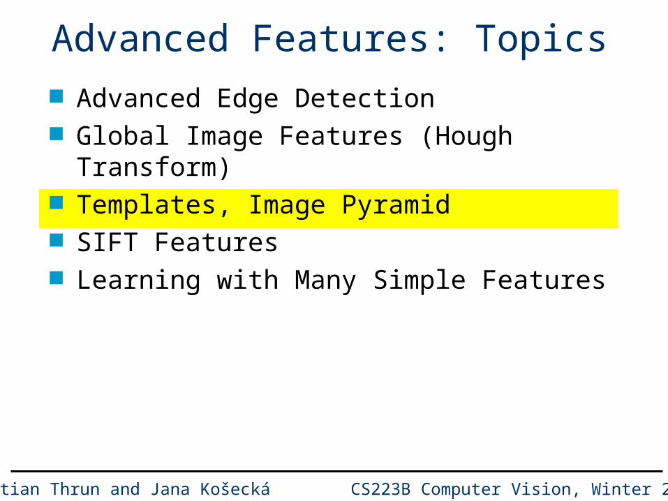
Advanced Features: Topics Advanced Edge Detection Global Image Features (Hough Transform) Templates, Image Pyramid SIFT Features Learning with Many Simple Features

Sebastian Thrun and Jana Košecká CS223B Computer Vision, Winter 2007
Features in Matlabim = imread('bridge.jpg');
bw = rgb2gray(im);
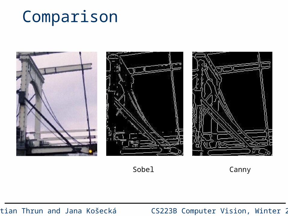
edge(im,’sobel’) - (almost) linear
edge(im,’canny’) - not local, no closed form

Sebastian Thrun and Jana Košecká CS223B Computer Vision, Winter 2007
Sobel Operator
-1 -2 -1 0 0 0 1 2 1
-1 0 1-2 0 2 -1 0 1
S1= S2 =
Edge Magnitude =
Edge Direction =
S1 + S22 2
tan-1S1
S2

Sebastian Thrun and Jana Košecká CS223B Computer Vision, Winter 2007
Sobel in Matlab
edge(im,’sobel’)

Sebastian Thrun and Jana Košecká CS223B Computer Vision, Winter 2007
Canny Edge Detector
edge(im,’canny’)
Sebastian Thrun and Jana Košecká CS223B Computer Vision, Winter 2007
Comparison
CannySobel

Sebastian Thrun and Jana Košecká CS223B Computer Vision, Winter 2007
Canny Edge Detection
Steps:1. Apply derivative of Gaussian
2. Non-maximum suppression• Thin multi-pixel wide “ridges” down to single pixel width
3. Linking and thresholding• Low, high edge-strength thresholds• Accept all edges over low threshold that are connected
to edge over high threshold
Sebastian Thrun and Jana Košecká CS223B Computer Vision, Winter 2007
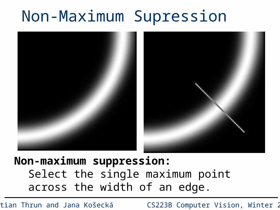
Non-Maximum Supression
Non-maximum suppression:Select the single maximum point across the width of an edge.

Sebastian Thrun and Jana Košecká CS223B Computer Vision, Winter 2007
Linking to the Next Edge Point
Assume the marked point q is an edge point.
Take the normal to the gradient at that point and use this to predict continuation points (either r or p).
Sebastian Thrun and Jana Košecká CS223B Computer Vision, Winter 2007
Edge Hysteresis
Hysteresis: A lag or momentum factor Idea: Maintain two thresholds khigh and klow
– Use khigh to find strong edges to start edge chain
– Use klow to find weak edges which continue edge chain
Typical ratio of thresholds is roughly
khigh / klow = 2

Sebastian Thrun and Jana Košecká CS223B Computer Vision, Winter 2007
Canny Edge Detection (Example)
courtesy of G. Loy
gap is gone
Originalimage
Strongedges
only
Strong +connectedweak edges
Weakedges

Sebastian Thrun and Jana Košecká CS223B Computer Vision, Winter 2007
Canny Edge Detection (Example)
Using Matlab with default thresholds

Sebastian Thrun and Jana Košecká CS223B Computer Vision, Winter 2007
Bridge Example Again
edge(im,’canny’)

Sebastian Thrun and Jana Košecká CS223B Computer Vision, Winter 2007
Corner Effects

Sebastian Thrun and Jana Košecká CS223B Computer Vision, Winter 2007
Summary: Canny Edge Detection Most commonly used method Traces edges, accommodates variations in
contrast Not a linear filter!
Problems with corners

Sebastian Thrun and Jana Košecká CS223B Computer Vision, Winter 2007
Advanced Features: Topics Advanced Edge Detection Global Image Features (Hough Transform) Templates, Image Pyramid SIFT Features Learning with Many Simple Features

Sebastian Thrun and Jana Košecká CS223B Computer Vision, Winter 2007
Towards Global Features
Local versus global

Sebastian Thrun and Jana Košecká CS223B Computer Vision, Winter 2007
Vanishing Points

Sebastian Thrun and Jana Košecká CS223B Computer Vision, Winter 2007
Vanishing Points

Sebastian Thrun and Jana Košecká CS223B Computer Vision, Winter 2007
Vanishing Points
A. Canaletto [1740], Arrival of the French Ambassador in Venice

Sebastian Thrun and Jana Košecká CS223B Computer Vision, Winter 2007
Vanishing Points…?
A. Canaletto [1740], Arrival of the French Ambassador in Venice

Sebastian Thrun and Jana Košecká CS223B Computer Vision, Winter 2007
From Edges to Lines

Sebastian Thrun and Jana Košecká CS223B Computer Vision, Winter 2007
Hough Transform
ymxb
y
x

Sebastian Thrun and Jana Košecká CS223B Computer Vision, Winter 2007
m
Hough Transform: Quantization
Detecting Lines by finding maxima / clustering in parameter space
b
mx
y

Sebastian Thrun and Jana Košecká CS223B Computer Vision, Winter 2007
Hough Transform: Algorithm For each image point, determine
– most likely line parameters b,m (direction of gradient)– strength (magnitude of gradient)
Increment parameter counter by strength value
Cluster in parameter space, pick local maxima

Sebastian Thrun and Jana Košecká CS223B Computer Vision, Winter 2007
Hough Transform: Results
Hough TransformImage Edge detection

Sebastian Thrun and Jana Košecká CS223B Computer Vision, Winter 2007
Summary Hough Transform Smart counting
– Local evidence for global features– Organized in a table– Careful with parameterization!
Problem: Curse of dimensionality– Works great for simple features with 3 unknowns– Will fail for complex objects
Problem: Not a local algorithm

Sebastian Thrun and Jana Košecká CS223B Computer Vision, Winter 2007
Advanced Features: Topics Advanced Edge Detection Global Image Features (Hough Transform) Templates, Image Pyramid SIFT Features Learning with Many Simple Features

Sebastian Thrun and Jana Košecká CS223B Computer Vision, Winter 2007
Features for Object Detection/Recognition
Want to find… in here

Sebastian Thrun and Jana Košecká CS223B Computer Vision, Winter 2007
Templates Find an object in an image!
We want Invariance!– Scaling– Rotation– Illumination– Perspective Projection

Sebastian Thrun and Jana Košecká CS223B Computer Vision, Winter 2007
Convolution with Templates% read imageim = imread('bridge.jpg');bw = double(im(:,:,1)) ./ 256;imshow(bw)
% apply FFTFFTim = fft2(bw);bw2 = real(ifft2(FFTim));imshow(bw2)
% define a kernelkernel=zeros(size(bw));kernel(1, 1) = 1;kernel(1, 2) = -1;FFTkernel = fft2(kernel);
% apply the kernel and check out the resultFFTresult = FFTim .* FFTkernel;result = real(ifft2(FFTresult));imshow(result)
% select an image patch
patch = bw(221:240,351:370);
imshow(patch)
patch = patch - (sum(sum(patch)) / size(patch,1) / size(patch, 2));
kernel=zeros(size(bw));
kernel(1:size(patch,1),1:size(patch,2)) = patch;
FFTkernel = fft2(kernel);
% apply the kernel and check out the result
FFTresult = FFTim .* FFTkernel;
result = max(0, real(ifft2(FFTresult)));
result = result ./ max(max(result));
result = (result .^ 1 > 0.5);
imshow(result)
% alternative convolution
imshow(conv2(bw, patch, 'same'))

Sebastian Thrun and Jana Košecká CS223B Computer Vision, Winter 2007
Template Convolution

Sebastian Thrun and Jana Košecká CS223B Computer Vision, Winter 2007
Template Convolution

Sebastian Thrun and Jana Košecká CS223B Computer Vision, Winter 2007
Aside: Convolution Theorem
)()()( gFIFgIF
2
)}(2exp{),(),))(,(( dydxvyuxiyxgvuyxgF Fourier Transform of g:
F is invertible

Sebastian Thrun and Jana Košecká CS223B Computer Vision, Winter 2007
Convolution with Templates% read imageim = imread('bridge.jpg');bw = double(im(:,:,1)) ./ 256;;imshow(bw)
% apply FFTFFTim = fft2(bw);bw2 = real(ifft2(FFTim));imshow(bw2)
% define a kernelkernel=zeros(size(bw));kernel(1, 1) = 1;kernel(1, 2) = -1;FFTkernel = fft2(kernel);
% apply the kernel and check out the resultFFTresult = FFTim .* FFTkernel;result = real(ifft2(FFTresult));imshow(result)
% select an image patch
patch = bw(221:240,351:370);
imshow(patch)
patch = patch - (sum(sum(patch)) / size(patch,1) / size(patch, 2));
kernel=zeros(size(bw));
kernel(1:size(patch,1),1:size(patch,2)) = patch;
FFTkernel = fft2(kernel);
% apply the kernel and check out the result
FFTresult = FFTim .* FFTkernel;
result = max(0, real(ifft2(FFTresult)));
result = result ./ max(max(result));
result = (result .^ 1 > 0.5);
imshow(result)
% alternative convolution
imshow(conv2(bw, patch, 'same'))

Sebastian Thrun and Jana Košecká CS223B Computer Vision, Winter 2007
Convolution with Templates Invariances:
– Scaling– Rotation– Illumination– Perspective Projection
Provides– Good localization
No
No
No
NoNo

Sebastian Thrun and Jana Košecká CS223B Computer Vision, Winter 2007
Scale Invariance: Image Pyramid

Sebastian Thrun and Jana Košecká CS223B Computer Vision, Winter 2007
Pyramid Convolution with Templates
Invariances:– Scaling– Rotation– Illumination– Perspective Projection
Provides– Good localization
No
Yes
No
NoNo
Sebastian Thrun and Jana Košecká CS223B Computer Vision, Winter 2007
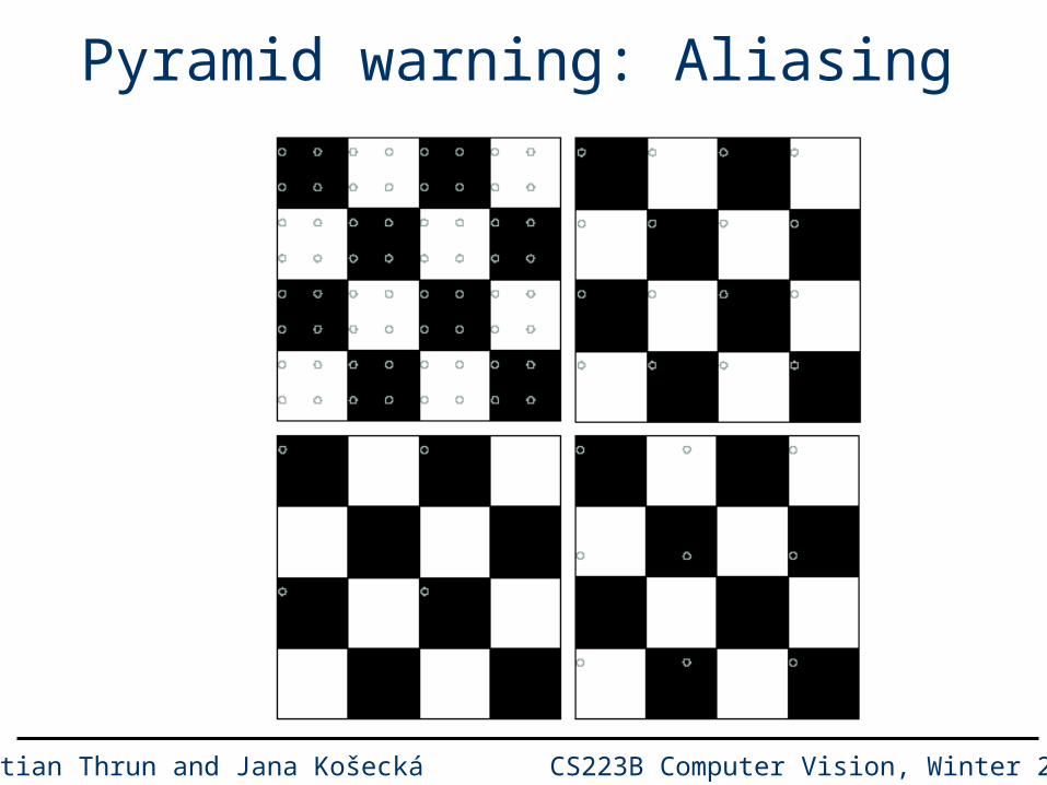
Pyramid warning: Aliasing

Sebastian Thrun and Jana Košecká CS223B Computer Vision, Winter 2007
Aliasing Effects
Constructing a pyramid by taking every second pixel leads to layers that badly misrepresent the top layer
Slide credit: Gary Bradski

Sebastian Thrun and Jana Košecká CS223B Computer Vision, Winter 2007
Solution to Aliasing Convolve with Gaussian

Sebastian Thrun and Jana Košecká CS223B Computer Vision, Winter 2007
Templates with Image Pyramid Invariance:
– Scaling– Rotation– Illumination– Perspective Projection
Provides– Good localization
No (maybe rotate template?)
Yes
No
Not reallyNo
Sebastian Thrun and Jana Košecká CS223B Computer Vision, Winter 2007
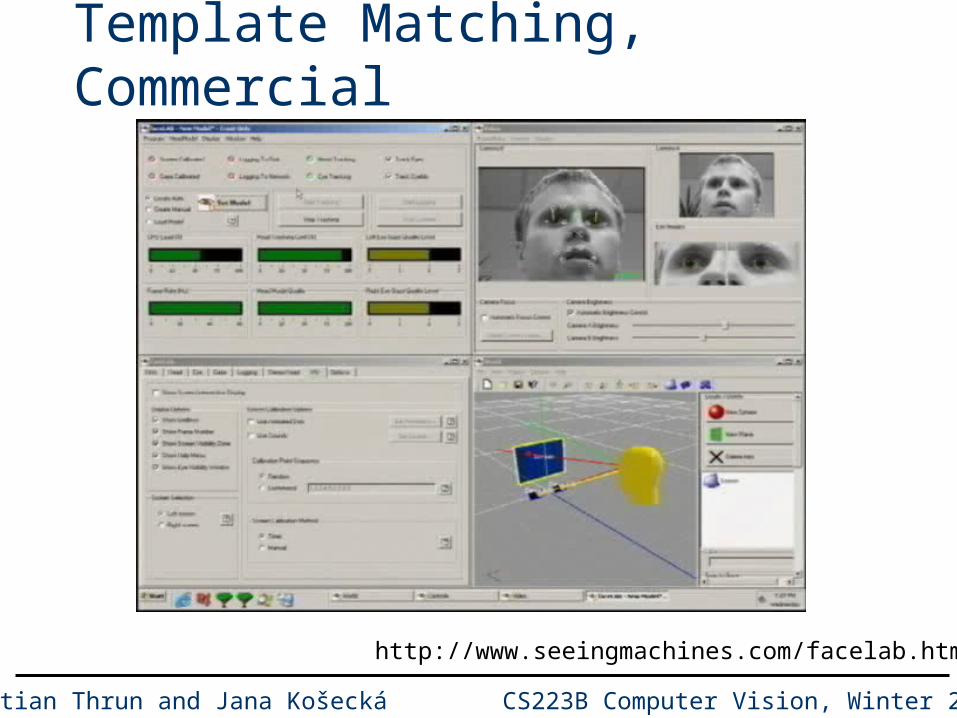
Template Matching, Commercial
http://www.seeingmachines.com/facelab.htm
Sebastian Thrun and Jana Košecká CS223B Computer Vision, Winter 2007
Advanced Features: Topics Advanced Edge Detection Global Image Features (Hough Transform) Templates, Image Pyramid SIFT Features Learning with Many Simple Features

Sebastian Thrun and Jana Košecká CS223B Computer Vision, Winter 2007
Improved Invariance Handling
Want to find… in here

Sebastian Thrun and Jana Košecká CS223B Computer Vision, Winter 2007
SIFT Features Invariances:
– Scaling– Rotation– Illumination– Deformation
Provides– Good localization
Yes
Yes
Yes
Not reallyYes
Sebastian Thrun and Jana Košecká CS223B Computer Vision, Winter 2007
SIFT Reference
Distinctive image features from scale-invariant keypoints. David G. Lowe, International Journal of Computer Vision, 60, 2 (2004), pp. 91-110.
SIFT = Scale Invariant Feature Transform

Sebastian Thrun and Jana Košecká CS223B Computer Vision, Winter 2007
Invariant Local Features Image content is transformed into local feature coordinates that are
invariant to translation, rotation, scale, and other imaging parameters
SIFT Features

Sebastian Thrun and Jana Košecká CS223B Computer Vision, Winter 2007
Advantages of invariant local features
Locality: features are local, so robust to occlusion and clutter (no prior segmentation)
Distinctiveness: individual features can be matched to a large database of objects
Quantity: many features can be generated for even small objects
Efficiency: close to real-time performance
Extensibility: can easily be extended to wide range of differing feature types, with each adding robustness
Sebastian Thrun and Jana Košecká CS223B Computer Vision, Winter 2007
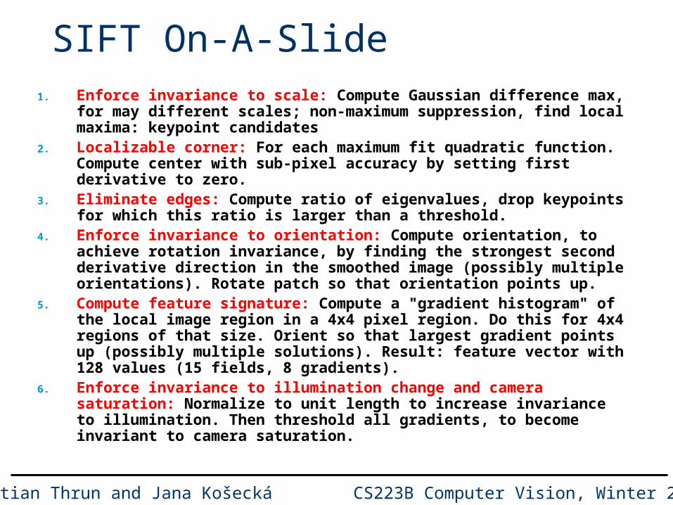
SIFT On-A-Slide1. Enforce invariance to scale: Compute Gaussian difference max, for may
different scales; non-maximum suppression, find local maxima: keypoint candidates
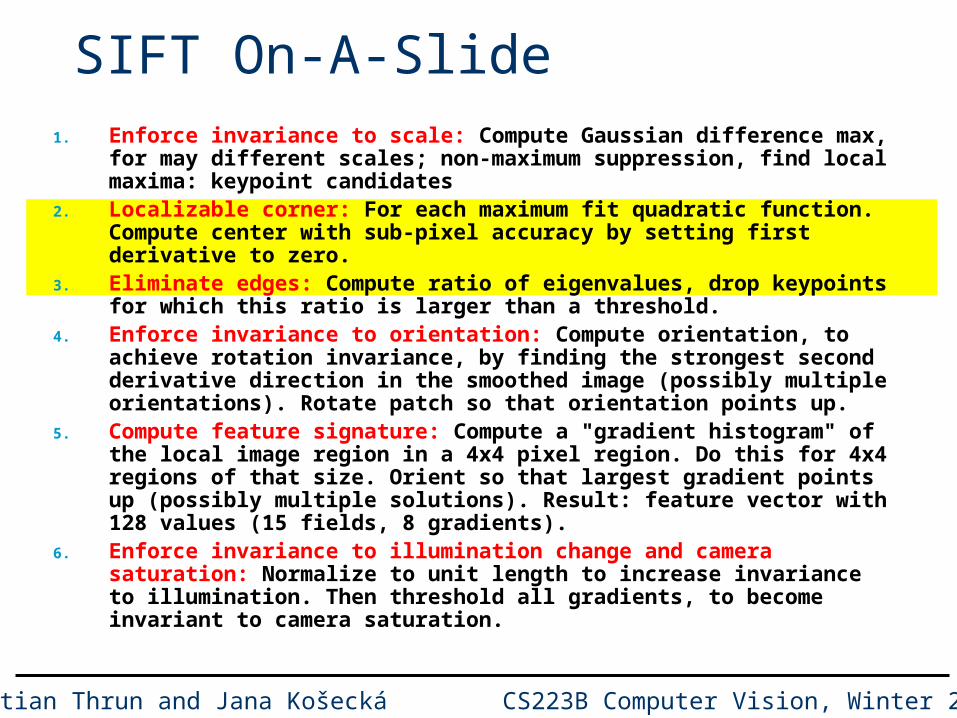
2. Localizable corner: For each maximum fit quadratic function. Compute center with sub-pixel accuracy by setting first derivative to zero.
3. Eliminate edges: Compute ratio of eigenvalues, drop keypoints for which this ratio is larger than a threshold.
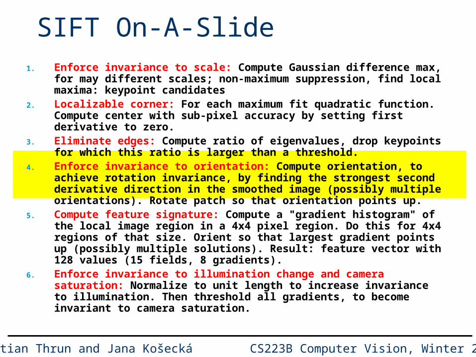
4. Enforce invariance to orientation: Compute orientation, to achieve rotation invariance, by finding the strongest second derivative direction in the smoothed image (possibly multiple orientations). Rotate patch so that orientation points up.
5. Compute feature signature: Compute a "gradient histogram" of the local image region in a 4x4 pixel region. Do this for 4x4 regions of that size. Orient so that largest gradient points up (possibly multiple solutions). Result: feature vector with 128 values (15 fields, 8 gradients).
6. Enforce invariance to illumination change and camera saturation: Normalize to unit length to increase invariance to illumination. Then threshold all gradients, to become invariant to camera saturation.

Sebastian Thrun and Jana Košecká CS223B Computer Vision, Winter 2007
SIFT On-A-Slide1. Enforce invariance to scale: Compute Gaussian difference max, for may
different scales; non-maximum suppression, find local maxima: keypoint candidates
2. Localizable corner: For each maximum fit quadratic function. Compute center with sub-pixel accuracy by setting first derivative to zero.
3. Eliminate edges: Compute ratio of eigenvalues, drop keypoints for which this ratio is larger than a threshold.
4. Enforce invariance to orientation: Compute orientation, to achieve rotation invariance, by finding the strongest second derivative direction in the smoothed image (possibly multiple orientations). Rotate patch so that orientation points up.
5. Compute feature signature: Compute a "gradient histogram" of the local image region in a 4x4 pixel region. Do this for 4x4 regions of that size. Orient so that largest gradient points up (possibly multiple solutions). Result: feature vector with 128 values (15 fields, 8 gradients).
6. Enforce invariance to illumination change and camera saturation: Normalize to unit length to increase invariance to illumination. Then threshold all gradients, to become invariant to camera saturation.

Sebastian Thrun and Jana Košecká CS223B Computer Vision, Winter 2007
Finding “Keypoints” (Corners)
Idea: Find Corners, but scale invariance
Approach: Run linear filter (diff of Gaussians) Do this at different resolutions of image pyramid
Sebastian Thrun and Jana Košecká CS223B Computer Vision, Winter 2007
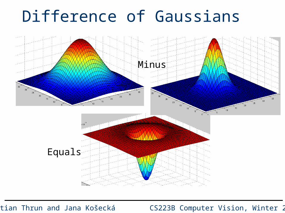
Difference of Gaussians
Minus
Equals
Sebastian Thrun and Jana Košecká CS223B Computer Vision, Winter 2007
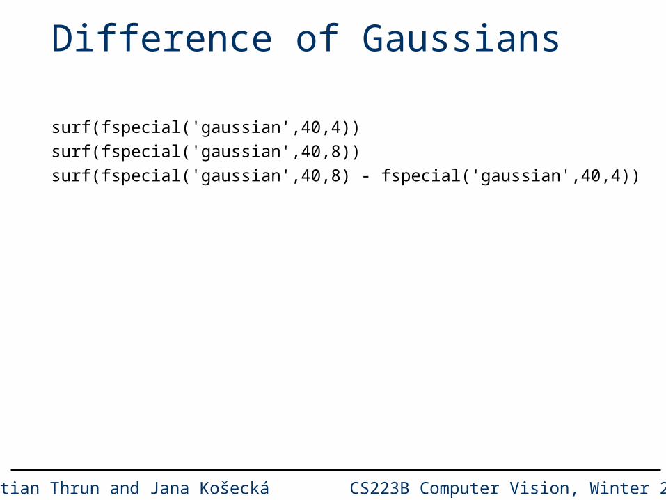
Difference of Gaussians
surf(fspecial('gaussian',40,4))
surf(fspecial('gaussian',40,8))
surf(fspecial('gaussian',40,8) - fspecial('gaussian',40,4))
Sebastian Thrun and Jana Košecká CS223B Computer Vision, Winter 2007
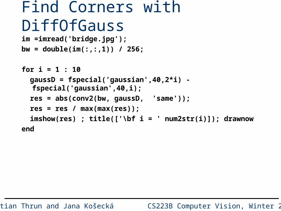
Find Corners with DiffOfGaussim =imread('bridge.jpg');
bw = double(im(:,:,1)) / 256;
for i = 1 : 10
gaussD = fspecial('gaussian',40,2*i) - fspecial('gaussian',40,i);
res = abs(conv2(bw, gaussD, 'same'));
res = res / max(max(res));
imshow(res) ; title(['\bf i = ' num2str(i)]); drawnow
end

Sebastian Thrun and Jana Košecká CS223B Computer Vision, Winter 2007
Gaussian Kernel Size i=1

Sebastian Thrun and Jana Košecká CS223B Computer Vision, Winter 2007
Gaussian Kernel Size i=2

Sebastian Thrun and Jana Košecká CS223B Computer Vision, Winter 2007
Gaussian Kernel Size i=3

Sebastian Thrun and Jana Košecká CS223B Computer Vision, Winter 2007
Gaussian Kernel Size i=4

Sebastian Thrun and Jana Košecká CS223B Computer Vision, Winter 2007
Gaussian Kernel Size i=5

Sebastian Thrun and Jana Košecká CS223B Computer Vision, Winter 2007
Gaussian Kernel Size i=6

Sebastian Thrun and Jana Košecká CS223B Computer Vision, Winter 2007
Gaussian Kernel Size i=7

Sebastian Thrun and Jana Košecká CS223B Computer Vision, Winter 2007
Gaussian Kernel Size i=8
Sebastian Thrun and Jana Košecká CS223B Computer Vision, Winter 2007
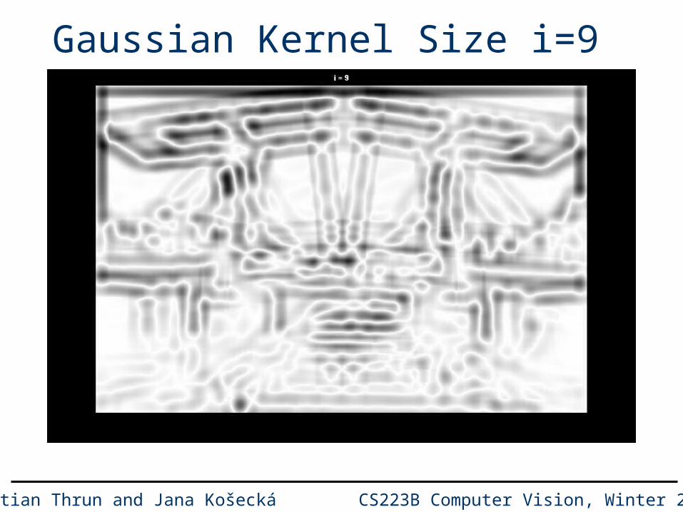
Gaussian Kernel Size i=9

Sebastian Thrun and Jana Košecká CS223B Computer Vision, Winter 2007
Gaussian Kernel Size i=10
Sebastian Thrun and Jana Košecká CS223B Computer Vision, Winter 2007
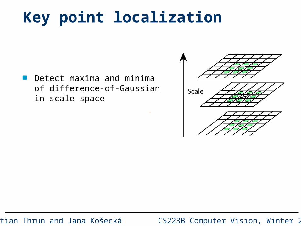
Key point localization
Detect maxima and minima of difference-of-Gaussian in scale space
B l u r
R e s a m p l e
S u b t r a c t

Sebastian Thrun and Jana Košecká CS223B Computer Vision, Winter 2007
Example of keypoint detection
(a) 233x189 image(b) 832 DOG extrema(c) 729 above threshold
Sebastian Thrun and Jana Košecká CS223B Computer Vision, Winter 2007
SIFT On-A-Slide1. Enforce invariance to scale: Compute Gaussian difference max, for may
different scales; non-maximum suppression, find local maxima: keypoint candidates
2. Localizable corner: For each maximum fit quadratic function. Compute center with sub-pixel accuracy by setting first derivative to zero.
3. Eliminate edges: Compute ratio of eigenvalues, drop keypoints for which this ratio is larger than a threshold.
4. Enforce invariance to orientation: Compute orientation, to achieve rotation invariance, by finding the strongest second derivative direction in the smoothed image (possibly multiple orientations). Rotate patch so that orientation points up.
5. Compute feature signature: Compute a "gradient histogram" of the local image region in a 4x4 pixel region. Do this for 4x4 regions of that size. Orient so that largest gradient points up (possibly multiple solutions). Result: feature vector with 128 values (15 fields, 8 gradients).
6. Enforce invariance to illumination change and camera saturation: Normalize to unit length to increase invariance to illumination. Then threshold all gradients, to become invariant to camera saturation.

Sebastian Thrun and Jana Košecká CS223B Computer Vision, Winter 2007
Example of keypoint detection
Threshold on value at DOG peak and on ratio of principle curvatures (Harris approach)
(c) 729 left after peak value threshold (from 832)(d) 536 left after testing ratio of principle curvatures
Sebastian Thrun and Jana Košecká CS223B Computer Vision, Winter 2007
SIFT On-A-Slide1. Enforce invariance to scale: Compute Gaussian difference max, for may
different scales; non-maximum suppression, find local maxima: keypoint candidates
2. Localizable corner: For each maximum fit quadratic function. Compute center with sub-pixel accuracy by setting first derivative to zero.
3. Eliminate edges: Compute ratio of eigenvalues, drop keypoints for which this ratio is larger than a threshold.
4. Enforce invariance to orientation: Compute orientation, to achieve rotation invariance, by finding the strongest second derivative direction in the smoothed image (possibly multiple orientations). Rotate patch so that orientation points up.
5. Compute feature signature: Compute a "gradient histogram" of the local image region in a 4x4 pixel region. Do this for 4x4 regions of that size. Orient so that largest gradient points up (possibly multiple solutions). Result: feature vector with 128 values (15 fields, 8 gradients).
6. Enforce invariance to illumination change and camera saturation: Normalize to unit length to increase invariance to illumination. Then threshold all gradients, to become invariant to camera saturation.

Sebastian Thrun and Jana Košecká CS223B Computer Vision, Winter 2007
Select canonical orientation Create histogram of local gradient
directions computed at selected scale
Assign canonical orientation at peak of smoothed histogram
Each key specifies stable 2D coordinates (x, y, scale, orientation)
0 2

Sebastian Thrun and Jana Košecká CS223B Computer Vision, Winter 2007
SIFT On-A-Slide1. Enforce invariance to scale: Compute Gaussian difference max, for may
different scales; non-maximum suppression, find local maxima: keypoint candidates
2. Localizable corner: For each maximum fit quadratic function. Compute center with sub-pixel accuracy by setting first derivative to zero.
3. Eliminate edges: Compute ratio of eigenvalues, drop keypoints for which this ratio is larger than a threshold.
4. Enforce invariance to orientation: Compute orientation, to achieve rotation invariance, by finding the strongest second derivative direction in the smoothed image (possibly multiple orientations). Rotate patch so that orientation points up.
5. Compute feature signature: Compute a "gradient histogram" of the local image region in a 4x4 pixel region. Do this for 4x4 regions of that size. Orient so that largest gradient points up (possibly multiple solutions). Result: feature vector with 128 values (15 fields, 8 gradients).
6. Enforce invariance to illumination change and camera saturation: Normalize to unit length to increase invariance to illumination. Then threshold all gradients, to become invariant to camera saturation.

Sebastian Thrun and Jana Košecká CS223B Computer Vision, Winter 2007
SIFT vector formation
Thresholded image gradients are sampled over 16x16 array of locations in scale space
Create array of orientation histograms 8 orientations x 4x4 histogram array = 128 dimensions
Sebastian Thrun and Jana Košecká CS223B Computer Vision, Winter 2007
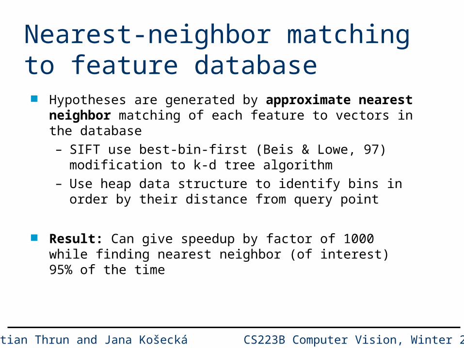
Nearest-neighbor matching to feature database
Hypotheses are generated by approximate nearest neighbor matching of each feature to vectors in the database – SIFT use best-bin-first (Beis & Lowe, 97) modification to k-d
tree algorithm– Use heap data structure to identify bins in order by their
distance from query point
Result: Can give speedup by factor of 1000 while finding nearest neighbor (of interest) 95% of the time

Sebastian Thrun and Jana Košecká CS223B Computer Vision, Winter 2007
3D Object Recognition
Extract outlines with background subtraction

Sebastian Thrun and Jana Košecká CS223B Computer Vision, Winter 2007
3D Object Recognition Only 3 keys are needed for
recognition, so extra keys provide robustness
Affine model is no longer as accurate

Sebastian Thrun and Jana Košecká CS223B Computer Vision, Winter 2007
Recognition under occlusion

Sebastian Thrun and Jana Košecká CS223B Computer Vision, Winter 2007
Test of illumination invariance Same image under differing illumination
273 keys verified in final match
Sebastian Thrun and Jana Košecká CS223B Computer Vision, Winter 2007
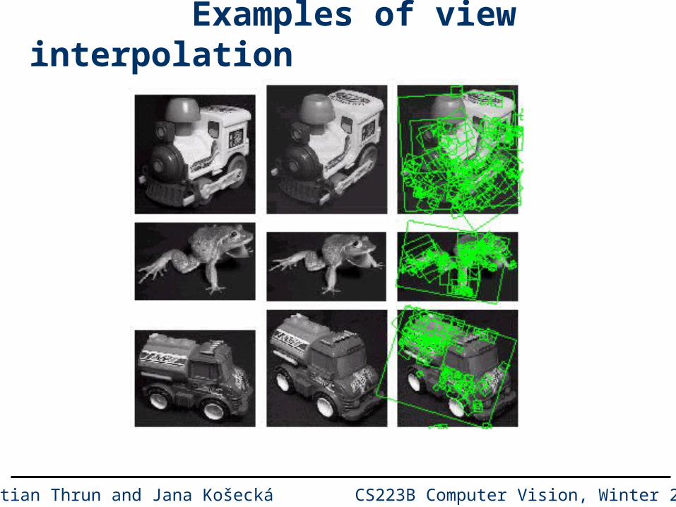
Examples of view interpolation

Sebastian Thrun and Jana Košecká CS223B Computer Vision, Winter 2007
Location recognition

Sebastian Thrun and Jana Košecká CS223B Computer Vision, Winter 2007
SIFT Invariances:
– Scaling– Rotation– Illumination– Perspective Projection
Provides– Good localization
YesYes
Yes
MaybeYes
Sebastian Thrun and Jana Košecká CS223B Computer Vision, Winter 2007
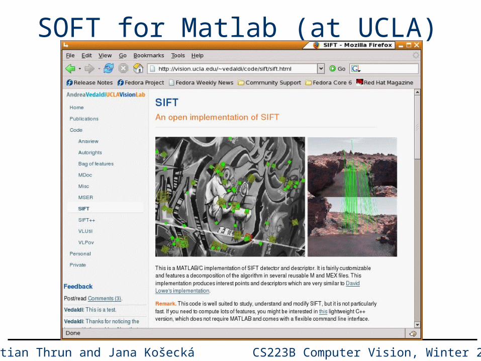
SOFT for Matlab (at UCLA)

Sebastian Thrun and Jana Košecká CS223B Computer Vision, Winter 2007
SIFT demos
Run
sift_compile
sift_demo2

Sebastian Thrun and Jana Košecká CS223B Computer Vision, Winter 2007
Summary SIFT1. Enforce invariance to scale: Compute Gaussian difference max, for may
different scales; non-maximum suppression, find local maxima: keypoint candidates
2. Localizable corner: For each maximum fit quadratic function. Compute center with sub-pixel accuracy by setting first derivative to zero.
3. Eliminate edges: Compute ratio of eigenvalues, drop keypoints for which this ratio is larger than a threshold.
4. Enforce invariance to orientation: Compute orientation, to achieve rotation invariance, by finding the strongest second derivative direction in the smoothed image (possibly multiple orientations). Rotate patch so that orientation points up.
5. Compute feature signature: Compute a "gradient histogram" of the local image region in a 4x4 pixel region. Do this for 4x4 regions of that size. Orient so that largest gradient points up (possibly multiple solutions). Result: feature vector with 128 values (15 fields, 8 gradients).
6. Enforce invariance to illumination change and camera saturation: Normalize to unit length to increase invariance to illumination. Then threshold all gradients, to become invariant to camera saturation.
Defines state-of-the-art in invariant feature matching!

Sebastian Thrun and Jana Košecká CS223B Computer Vision, Winter 2007
Advanced Features: Topics Advanced Edge Detection Global Image Features (Hough Transform) Templates, Image Pyramid SIFT Features Learning with Many Simple Features

Sebastian Thrun and Jana Košecká CS223B Computer Vision, Winter 2007
A totally different idea Use many very simple features Learn cascade of tests for target object Efficient if:
– features easy to compute– cascade short

Sebastian Thrun and Jana Košecká CS223B Computer Vision, Winter 2007
Using Many Simple Features Viola Jones / Haar Features
(Generalized) Haar Features:
• rectangular blocks, white or black• 3 types of features:
• two rectangles: horizontal/vertical• three rectangles• four rectangles
• in 24x24 window: 180,000 possible features

Sebastian Thrun and Jana Košecká CS223B Computer Vision, Winter 2007
Integral ImageDef: The integral image at location (x,y), is the sum of the pixel values above and to the left of (x,y), inclusive.
We can calculate the integral image representation of
the image in a single pass.
(x,y)
s(x,y) = s(x,y-1) + i(x,y)
ii(x,y) = ii(x-1,y) + s(x,y)
(0,0)
x
y
Slide credit: Gyozo Gidofalvi

Sebastian Thrun and Jana Košecká CS223B Computer Vision, Winter 2007
Efficient Computation of Rectangle Value
Using the integral image representation one can compute the value of any rectangular sum in constant time.
Example: Rectangle D
ii(4) + ii(1) – ii(2) – ii(3)
As a result two-, three-, and four-rectangular features can be computed with 6, 8 and 9 array references respectively.
Slide credit: Gyozo Gidofalvi

Sebastian Thrun and Jana Košecká CS223B Computer Vision, Winter 2007
Idea 1: Linear Separator
Slide credit: Frank Dellaert, Paul Viola, Foryth&Ponce

Sebastian Thrun and Jana Košecká CS223B Computer Vision, Winter 2007
Linear Separator for Image features(highly related to Vapnik’s Support Vector Machines)
Slide credit: Frank Dellaert, Paul Viola, Foryth&Ponce

Sebastian Thrun and Jana Košecká CS223B Computer Vision, Winter 2007
Problem How to find hyperplane? How to avoid evaluating 180,000 features?
Answer: Boosting [AdaBoost, Freund/Shapire]– Finds small set of features that are “sufficient”– Generalizes very well (a lot of max-margin theory)– Requires positive and negative examples

Sebastian Thrun and Jana Košecká CS223B Computer Vision, Winter 2007
AdaBoost Idea (in Viola/Jones): Given set of “weak” classifiers:
– Pick best one– Reweight training examples, so that misclassified
images have larger weight– Reiterate; then linearly combine resulting classifiers
Weak classifiers: Haar features

Sebastian Thrun and Jana Košecká CS223B Computer Vision, Winter 2007
AdaBoost Weak Classifier 1
WeightsIncreased
Weak classifier 3
Final classifier is linear combination of weak classifiers
t
xhyt
t Z
eiDiD
iti )(
1
)()(
t
i
xhyt
ht
Z
eiDh ii )()(min
Weak Classifier 2
Freund & Shapire

Sebastian Thrun and Jana Košecká CS223B Computer Vision, Winter 2007
Adaboost AlgorithmFreund & Shapire

Sebastian Thrun and Jana Košecká CS223B Computer Vision, Winter 2007
AdaBoost gives efficient classifier:
Features = Weak Classifiers Each round selects the optimal feature
given:– Previous selected features– Exponential Loss
AdaBoost Surprise– Generalization error decreases even after all
training examples 100% correctly classified (margin maximization phenomenon)

Sebastian Thrun and Jana Košecká CS223B Computer Vision, Winter 2007
Boosted Face Detection: Image Features
“Rectangle filters”
000,000,6100000,60 Unique Binary Features
Slide credit: Frank Dellaert, Paul Viola, Foryth&Ponce

Sebastian Thrun and Jana Košecká CS223B Computer Vision, Winter 2007
Example Classifier for Face Detection
ROC curve for 200 feature classifier
A classifier with 200 rectangle features was learned using AdaBoost
95% correct detection on test set with 1 in 14084false positives.
Slide credit: Frank Dellaert, Paul Viola, Foryth&Ponce

Sebastian Thrun and Jana Košecká CS223B Computer Vision, Winter 2007
Classifier are Efficient
Given a nested set of classifier hypothesis classes
vs false neg determined by
% False Pos
% D
etec
tion
0 50
50
100
IMAGESUB-WINDOW
Classifier 1
F
NON-FACE
F
NON-FACE
FACEClassifier 3T
F
NON-FACE
TTTClassifier 2
F
NON-FACE
Slide credit: Frank Dellaert, Paul Viola, Foryth&Ponce
Sebastian Thrun and Jana Košecká CS223B Computer Vision, Winter 2007
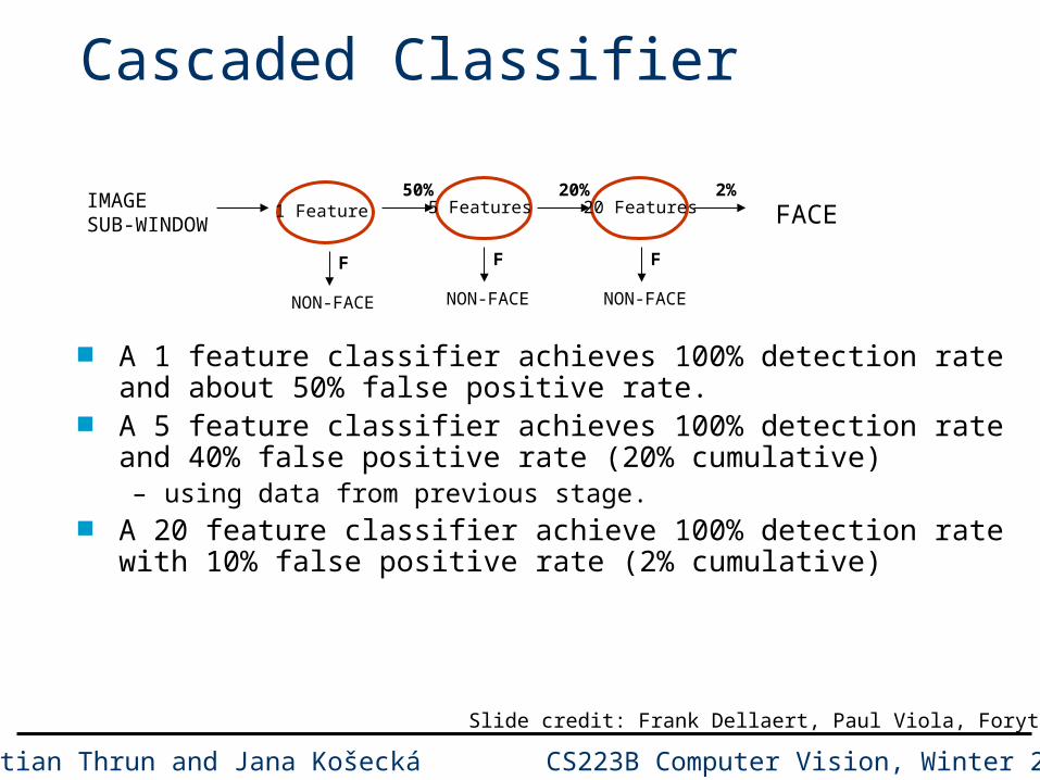
Cascaded Classifier
1 Feature 5 Features
F
50%20 Features
20% 2%
FACE
NON-FACE
F
NON-FACE
F
NON-FACE
IMAGESUB-WINDOW
A 1 feature classifier achieves 100% detection rate and about 50% false positive rate.
A 5 feature classifier achieves 100% detection rate and 40% false positive rate (20% cumulative)– using data from previous stage.
A 20 feature classifier achieve 100% detection rate with 10% false positive rate (2% cumulative)
Slide credit: Frank Dellaert, Paul Viola, Foryth&Ponce

Sebastian Thrun and Jana Košecká CS223B Computer Vision, Winter 2007
Output of Face Detector on Test Images
Slide credit: Frank Dellaert, Paul Viola, Foryth&Ponce

Sebastian Thrun and Jana Košecká CS223B Computer Vision, Winter 2007
Solving other “Face” Tasks
Facial Feature Localization
DemographicAnalysis
Profile Detection
Slide credit: Frank Dellaert, Paul Viola, Foryth&Ponce

Sebastian Thrun and Jana Košecká CS223B Computer Vision, Winter 2007
Face Localization Features Learned features reflect the task
Slide credit: Frank Dellaert, Paul Viola, Foryth&Ponce

Sebastian Thrun and Jana Košecká CS223B Computer Vision, Winter 2007
Face Profile Detection
Slide credit: Frank Dellaert, Paul Viola, Foryth&Ponce

Sebastian Thrun and Jana Košecká CS223B Computer Vision, Winter 2007
Face Profile Features

Sebastian Thrun and Jana Košecká CS223B Computer Vision, Winter 2007
Finding Cars (DARPA Urban Challenge) Hand-labeled images of generic car rear-ends Training time: ~5 hours, offline
1100 images
Credit: Hendrik Dahlkamp

Sebastian Thrun and Jana Košecká CS223B Computer Vision, Winter 2007
Generating even more examples Generic classifier finds all cars in recorded video. Compute offline and store in database
28700 images
Credit: Hendrik Dahlkamp

Sebastian Thrun and Jana Košecká CS223B Computer Vision, Winter 2007
Results - Video
Sebastian Thrun and Jana Košecká CS223B Computer Vision, Winter 2007
Summary Viola-Jones Many simple features
– Generalized Haar features (multi-rectangles)– Easy and efficient to compute
Discriminative Learning: – finds a small subset for object recognition– Uses AdaBoost
Result: Feature Cascade– 15fps on 700Mhz Laptop (=fast!)
Applications– Face detection– Car detection– Many others