STANDARDIZED CPUE FROM THE ROD AND REEL … · STANDARDIZED CPUE FROM THE ROD AND REEL AND . SMALL...
17
SCRS/2014/065 Collect. Vol. Sci. Pap. ICCAT, 71(5): 2239-2255 (2015) STANDARDIZED CPUE FROM THE ROD AND REEL AND SMALL SCALE GILLNET FISHERIES OF LA GUAIRA, VENEZUELA Elizabeth A. Babcock 1 , Freddy Arocha 2 SUMMARY Catches of sailfish (Istiophorus albicans), white marlin (Tetrapturus albidus) and blue marlin (Makaira nigricans) and effort data were available from the recreational rod and reel fishery based at the Playa Grande Yacht Club, Central Venezuela, from 1961 to 2001. Data were also available from a small-scale gillnet fishery in the same area from 1991 to 2012. Each dataset was standardized independently using a generalized linear mixed model (GLMM). The two datasets were also combined in a GLMM analysis that included the year, season, fishery and some two-way interactions as potential explanatory variables. The combined analysis produced a CPUE index of abundance that runs from 1961 to 2012. The index shows a decline followed by a period of stability for both sailfish and white marlin. The blue marlin index shows no trend. RÉSUMÉ Les prises de voiliers (Istiophorus albicans), de makaire blanc (Tetrapturus albidus) et de makaire bleu (Makaira nigricans) et les données d'effort étaient disponibles de la pêcherie récréative de canne et moulinet, basée à Playa Grande Yacht Club, au centre du Venezuela, de 1961 à 2001. Les données étaient également disponibles de la pêcherie de petits métiers opérant aux filets maillants dans la même zone de 1991 à 2012. Chaque jeu de données a été standardisé indépendamment à l'aide d'un modèle linéaire mixte généralisé (GLMM). Les deux jeux de données ont également été combinés dans une analyse de GLMM qui comprenait l'année, la saison, la pêcherie et une interaction à double sens, comme variables explicatives possibles. L'analyse combinée produit un indice d'abondance de la CPUE qui s'étend de 1961 à 2012. L'indice montre une diminution suivie d'une période de stabilité pour les voiliers et le makaire blanc. L'indice du makaire bleu ne dégage aucune tendance. RESUMEN Se disponía de datos de captura y esfuerzo de pez vela (Istiophorus albicans), aguja blanca (Tetrapturus albidus) y aguja azul (Makaira nigricans) de la pesquería de recreo de caña y carrete con base en el Playa Grande Yacht Club, Venezuela central, desde 1961 hasta 2001. Se disponía también de datos de una pesquería de redes de enmalle de pequeña escala en la misma zona para 1991-2012. Cada conjunto de datos se estandarizó de forma independiente utilizando un modelo lineal mixto generalizado (GLMM). Los dos conjuntos de datos se combinaron también en un análisis GLMM que incluía el año, la temporada, la pesquería y algunas interacciones de dos direcciones como posibles variables explicativas. El análisis combinado produjo un índice de abundancia de CPUE que va desde 1961 a 2012. El índice muestra un descenso seguido de un periodo de estabilidad tanto para el pez vela como para la aguja blanca. El índice para la aguja azul no muestra ninguna tendencia. KEYWORDS Catch/effort, Mathematical models 1 Department of Marine Biology and Ecology, Rosenstiel School of Marine and Atmospheric Science, University of Miami, 4600 Rickenbacker Cswy., Miami, FL 33149. USA. [email protected] 2 DBP-IOV-UDO. Cumaná-Venezuela. 2239
Transcript of STANDARDIZED CPUE FROM THE ROD AND REEL … · STANDARDIZED CPUE FROM THE ROD AND REEL AND . SMALL...
SCRS/2014/065 Collect. Vol. Sci. Pap. ICCAT, 71(5): 2239-2255 (2015)
STANDARDIZED CPUE FROM THE ROD AND REEL AND
SMALL SCALE GILLNET FISHERIES OF LA GUAIRA, VENEZUELA
Elizabeth A. Babcock1, Freddy Arocha2
SUMMARY
Catches of sailfish (Istiophorus albicans), white marlin (Tetrapturus albidus) and blue marlin
(Makaira nigricans) and effort data were available from the recreational rod and reel fishery
based at the Playa Grande Yacht Club, Central Venezuela, from 1961 to 2001. Data were also
available from a small-scale gillnet fishery in the same area from 1991 to 2012. Each dataset
was standardized independently using a generalized linear mixed model (GLMM). The two
datasets were also combined in a GLMM analysis that included the year, season, fishery and
some two-way interactions as potential explanatory variables. The combined analysis produced
a CPUE index of abundance that runs from 1961 to 2012. The index shows a decline followed
by a period of stability for both sailfish and white marlin. The blue marlin index shows no
trend.
RÉSUMÉ
Les prises de voiliers (Istiophorus albicans), de makaire blanc (Tetrapturus albidus) et de
makaire bleu (Makaira nigricans) et les données d'effort étaient disponibles de la pêcherie
récréative de canne et moulinet, basée à Playa Grande Yacht Club, au centre du Venezuela, de
1961 à 2001. Les données étaient également disponibles de la pêcherie de petits métiers
opérant aux filets maillants dans la même zone de 1991 à 2012. Chaque jeu de données a été
standardisé indépendamment à l'aide d'un modèle linéaire mixte généralisé (GLMM). Les deux
jeux de données ont également été combinés dans une analyse de GLMM qui comprenait
l'année, la saison, la pêcherie et une interaction à double sens, comme variables explicatives
possibles. L'analyse combinée produit un indice d'abondance de la CPUE qui s'étend de 1961 à
2012. L'indice montre une diminution suivie d'une période de stabilité pour les voiliers et le
makaire blanc. L'indice du makaire bleu ne dégage aucune tendance.
RESUMEN
Se disponía de datos de captura y esfuerzo de pez vela (Istiophorus albicans), aguja blanca
(Tetrapturus albidus) y aguja azul (Makaira nigricans) de la pesquería de recreo de caña y
carrete con base en el Playa Grande Yacht Club, Venezuela central, desde 1961 hasta 2001. Se
disponía también de datos de una pesquería de redes de enmalle de pequeña escala en la
misma zona para 1991-2012. Cada conjunto de datos se estandarizó de forma independiente
utilizando un modelo lineal mixto generalizado (GLMM). Los dos conjuntos de datos se
combinaron también en un análisis GLMM que incluía el año, la temporada, la pesquería y
algunas interacciones de dos direcciones como posibles variables explicativas. El análisis
combinado produjo un índice de abundancia de CPUE que va desde 1961 a 2012. El índice
muestra un descenso seguido de un periodo de estabilidad tanto para el pez vela como para la
aguja blanca. El índice para la aguja azul no muestra ninguna tendencia.
KEYWORDS
Catch/effort, Mathematical models
1 Department of Marine Biology and Ecology, Rosenstiel School of Marine and Atmospheric Science, University of Miami, 4600
Rickenbacker Cswy., Miami, FL 33149. USA. [email protected] 2 DBP-IOV-UDO. Cumaná-Venezuela.
2239

1. Introduction
The fishing site known as Placer de la Guaira, off Venezuela, has been a known hot-spot for billfishes since the
1960s. Data are available from 1961 to 2001 on the number of rod and rod and reel fishing trips taken each
month from the Playa Grande Yacht Club, and the number of sailfish, white marlin and blue marlin caught in
each month. Gaertner and Alio (1997) evaluated trends in this dataset from 1961 to 1995 for all three billfish
species and found apparent declines in all three species. Beginning in 1991, this fishery was required to release
all billfish caught, so the records are less complete in the 1990s, and there are no records after 2001. A dataset is
also available from the small-scale gillnet fishery that operates in the same area, from 1991 to 2012. This dataset
includes the number of sets and the monthly total catch in kg of all three billfish species. Arocha et al. (2008)
standardized the gillnet fishery data to calculate an index of abundance for sailfish, and found no trend over time.
The objective off this paper is to provide updated series for both the rod and reel and the gillnet fishery. In
addition, we produce a combined index that includes the data from both fisheries. Because the two fisheries
operate in the same area, they should give similar abundance trends. Considering that the rod and reel fishery
data are not available since 2001, it would be useful to combine the two series to get a longer time trend in
abundance.
2. Methods
For both the rod and reel fishery and the gillnet fishery, and for the two datasets combined, the data were
standardized using a generalized linear mixed model (GLMM). The response variable was log(CPUE+0.01) for
either sailfish, white marlin or blue marlin. The constant was added because there were some zero observations.
However, because the available data were monthly summaries, there were not enough few zero observations to
require a delta model to be used. For the rod and reel fishery, CPUE was in numbers caught per trip. For the
gillnet fishery, CPUE was in kilograms caught per set. For the combined analysis, both CPUE data sets were
divided by their mean in 1991 to 2001 in order to make the units approximately comparable. The explanatory
variables were year, season (Winter: December-February, Spring: March-May, Summer: June-August, Autumn:
September-November), and the interaction between year and season. For the analysis that included both
fisheries, fishery was an explanatory variable, along with a fishery × season interaction. It was not possible to
include an interaction between fishery and year because most years only had data from one fishery. Season and
any interactions were treated as random effects, while year and fishery were fixed effects. Explanatory variables
were included in the model if they were supported by the Akaike information criterion (AIC) and the Bayesian
information criterion (BIC), and if they explained more than 5% of the model deviance (Ortiz and Arocha 2004).
All analyses were conducted in R version 3.01 (R Core Team 2013).
3. Results
The rod and reel fishery has complete records between 1961 and 1989 (Table 1). From 1991 to 2001, there are
records for some months in each year, but many months have no recorded catches. The gillnet fishery data are
incomplete in 1991, but contain records for all months in every year from 1992 to 2012. Despite the fact that
many months are missing, the total effort in the rod and reel fishery, in number of trips, is as high in the 1990s as
it has ever been (Figure 1).
For both the rod and reel and the gillnet fishery, there were consistent seasonal trends in CPUE for all three
species (Figure 2). In both fisheries, white marlin were more commonly caught in the second half of the year,
and blue marlin in the first half of the year. The trend in sailfish catch rates was not as consistent between the
two fisheries. The monthly catch rates appeared to be lognormally distributed in both fisheries for all three
species, with the exception of blue marlin, which had a large number of zero observations in the rod and reel
fishery (Figure 3).
2240

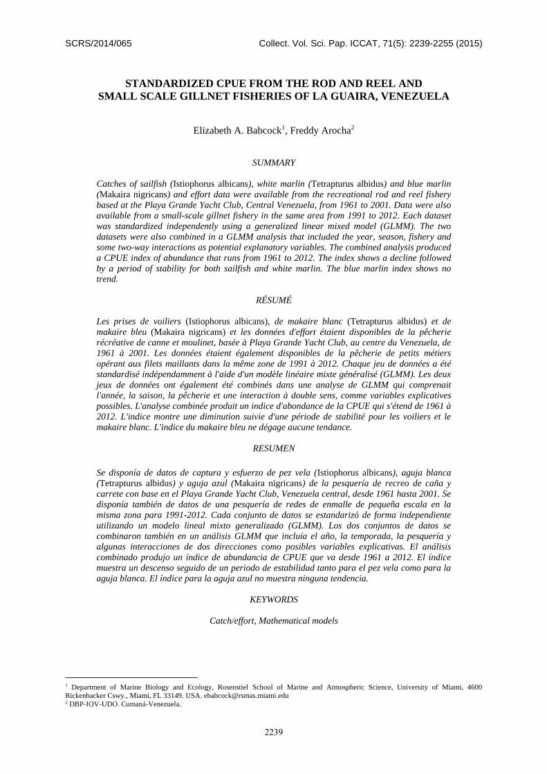
For all three species in the rod and reel fishery the BIC and AIC both preferred a model with both year and
season effects, and in some cases an interaction between year and season (Table 2a). Nevertheless, the year
effect explained the majority of the deviance (Table 2b). Using the AIC best model, which included an
interaction term for sailfish and white marlin, but not blue marlin, the residuals seem to be fairly normally
distributed (Figure 4). The predictions from the best fit models (Figure 5) are very similar to the raw CPUE if
the raw CPUE is calculated using a lognormal estimator (i.e. the mean of the log(CPUE) converted back to
normal). The trend in the GLMM-standardized CPUE is rather flat compared to the raw arithmetic means,
because the arithmetic mean is more influenced by the few large CPUE values in the late 1960s and early 1970s.
The previous analyses of the rod and reel fishery (Gaertner and Alio 1994, 1998) adjusted the effort in each trip
by the number of fish caught, on the assumption that anglers on a boat would have to stop fishing when someone
was fighting a fish. However, the average CPUE is quite similar with or without the adjustment (Figure 5).
For the gillnet fishery, both AIC and BIC preferred models with both the year and season effects, for all three
species. For blue marlin, both criteria preferred models that included the interaction term as well (Table 3). Year
explained more than 90% of the deviance for both sailfish and blue marlin, but only 45% of the deviance for
white marlin. The diagnostics (Figure 6) show generally normal residuals, except for some outliers at low
predicted values. The standardized CPUE index looked very similar to the raw arithmetic mean, or the raw
lognormal mean, and was also very similar to the values calculated by Arocha et al. (2008) for sailfish
(Figure 7).
When both datasets were combined, the AIC preferred the model with effects of year, fishery, season and the
interaction between fishery and season for sailfish and white marlin (Table 4a). That fishery was included in the
AIC best model was surprising, because fishery explained less than 2% of the deviance for either species
(Table 4b). For blue marlin, the AIC preferred the model with only year and season. For all three species, much
of the deviance was explained by the interaction between year and season, perhaps because of changes over time
in the seasonal trend in abundance. The diagnostics of the AIC preferred models looked fairly normal (Figure 8),
except for some outliers at low predicted values. The predicted values of the index look very low and flat over
the recent time period for all three species (Figure 9). Combining the data from the two sources gives very
similar trends to what would be obtained by fitting the two series separately and dividing them by their mean in
the time period when they overlap (Figure 10). However, the standard errors are somewhat higher in recent
years for the artisanal fishery than for the two datasets combined (Table 5).
4. Discussion
Because La Guaira is a billfish hotspot, catch rates from the area may provide a useful index of abundance.
Given that the rod and reel dataset has not been continued since 2001, it would be useful to be able to combine
the two datasets to estimate a long term index of abundance. Combining the two indices requires several
assumptions. First, the average weight must be assumed to be constant in each fishery over time, so that CPUE
in numbers in the rod and reel fishery are directly proportional to CPUE in weight in the gillnet fishery. This is a
reasonable assumption because the rod and reel fishery did not select for a specific size of fish, and the average
size of fish in the gillnet fishery has not changed over time.
Second, although the two fisheries may have different catchabilities, both catchabilities must be constant over
time. Because information is not available on vessel characteristics such boat size, gear used, time spent fishing,
or targeting in either fishery, these variables could not be added to the standardization. Any change in fishing
methods over time in either fishery would bias the index. It is known that fishing methodology in the gillnet
fishery has not changed over time (Arocha et al. 2008). Whether rod and reel fishermen have become more
efficient over time is not known.
Third, the combined GLMM makes the assumption that the error structure in the two fisheries is comparable.
This may not be a good assumption, because catch rates are more variable in the rod and reel fishery than the
artisanal gillnet fishery. For this reason, it may be preferable to model the fisheries separately if they are to be
used in a stock assessment model that uses the variances of the indices as an input (Table 5).
2241

Finally, whether modeling the two fisheries separately or together, the scaling of the two fisheries depends on the
CPUE in the years when both data sets overlap. In the combined model presented here, the CPUE data were
rescaled by dividing each dataset by its mean in the 1990s. The model was also given the opportunity to estimate
the scaling factor between the two datasets, in the main effect of “fishery” in the GLMM. If the two series were
standardized independently and input into a stock assessment model, the model would be able to estimate the
scaling factor by estimating a different catchability for fishery. In either a combined GLMM or a stock
assessment using both series, the relative scaling depends on the assumption that the CPUE in the rod and reel
fishery in the 1990s is comparable to the CPUE in the rod and reel fishery before 1990. Thus, the results are
highly dependent on what assumptions are made about the missing data in the 1990s in the rod and reel fishery
(Table 1). Considering that in 1991 there was a ban on retention of billfishes in the rod and reel fishery, it is
quite possible that total catch in the 1990s is under-reported because billfishes are more likely to be released at
sea. The analyses presented here left out months with no recorded catches. Thus, if some of the months with no
reported catches actually had a catch of zero for a billfish species, the rod and reel CPUE in the 1990s could be
overestimated. Conversely, if the reported catches in months with data are an underestimate of the true catch,
then the CPUE in the 1990s could be underestimated. Future analyses of these datasets may consider using some
kind of imputation model to deal with the missing data in this period. Considering that the effort in the rod and
reel fishery did not decline after the ban on retaining billfishes, it seems likely that large numbers of billfish
continue to be caught and released.
References
Arocha, F., M. Ortiz, A. Bárrios, D. Debrot and L.A. Marcano. 2008. Catch rates for sailfish (Istiophorus
albicans) from the small scale drift gillnet fishery off La Guaira, Venezuela: Period 1991-2007. Collect. Vol.
Sci. Pap. ICCAT, 64(6): 1844-1853.
Ortiz, M. and Arocha, F. 2004. Alternative error distribution models for standardization of catch rates of non-
target species from a pelagic longline fishery: billfish species in the Venezuelan tuna longline fishery.
Fisheries Research 70:275-297.
Gaertner, G. and J.J. Alio. 1998. Trends in the recreational billfish fishery CPUE off Playa Grande (1961-1995),
Central Venezuelan Coast. Col. Vol. Sci. Pap. ICCAT 47: 289-300.
Gaertner, G. and J.J. Alio. 1994. Changes in apparent indices of billfishes in the Venezuelan recreational fishery
of Playa Granda (1961-1990), Central Venezuelan Coast Col. Vol. Sci. Pap. ICCAT 41: 473-489.
R Core Team. 2013 R: A language and environment for statistical computing. R Foundation for Statistical
Computing, Vienna, Austria. www.R-project.org/.
2242

Table 1. Number of months with effort data and catch data for each speces available for each dataset in each
year.
RR Gillnet RR Gillnet
Yr Eff SAI WHM BUM Eff SAI WHM BUM Yr Eff SAI WHM BUM Eff SAI WHM BUM
61 12 12 12 12 0 0 0 0 87 12 12 12 12 0 0 0 0
62 12 12 12 12 0 0 0 0 88 12 12 12 12 0 0 0 0
63 12 12 12 12 0 0 0 0 89 12 12 12 12 0 0 0 0
64 12 12 12 12 0 0 0 0 90 0 0 0 0 0 0 0 0
65 12 12 12 12 0 0 0 0 91 12 8 9 10 12 7 10 10
66 12 12 12 12 0 0 0 0 92 9 11 10 11 12 12 12 12
67 12 12 12 12 0 0 0 0 93 12 0 3 5 12 12 12 12
68 12 12 12 12 0 0 0 0 94 12 5 9 7 12 12 12 12
69 12 12 12 12 0 0 0 0 95 12 4 7 8 12 12 12 12
70 12 12 12 12 0 0 0 0 96 12 4 1 12 12 12 12 12
71 12 12 12 12 0 0 0 0 97 12 4 8 9 12 12 12 12
72 12 12 12 12 0 0 0 0 98 12 2 1 6 12 12 12 12
73 12 12 12 12 0 0 0 0 99 12 3 3 4 12 12 12 12
74 12 12 12 12 0 0 0 0 00 12 1 3 4 12 12 12 12
75 12 12 12 12 0 0 0 0 01 11 3 4 8 12 12 12 12
76 12 12 12 12 0 0 0 0 02 0 0 0 0 12 12 12 12
77 12 12 12 12 0 0 0 0 03 0 0 0 0 12 12 12 12
78 12 12 12 12 0 0 0 0 04 0 0 0 0 12 12 12 12
79 12 12 12 12 0 0 0 0 05 0 0 0 0 12 12 12 12
80 12 12 12 12 0 0 0 0 06 0 0 0 0 12 12 12 12
81 12 12 12 12 0 0 0 0 07 0 0 0 0 12 12 12 12
82 12 12 12 12 0 0 0 0 08 0 0 0 0 12 12 12 12
83 12 12 12 12 0 0 0 0 09 0 0 0 0 12 12 12 12
84 12 12 12 12 0 0 0 0 10 0 0 0 0 12 12 12 12
85 12 12 12 12 0 0 0 0 11 0 0 0 0 12 12 12 12
86 12 12 12 12 0 0 0 0 12 0 0 0 0 12 12 12 12
2243
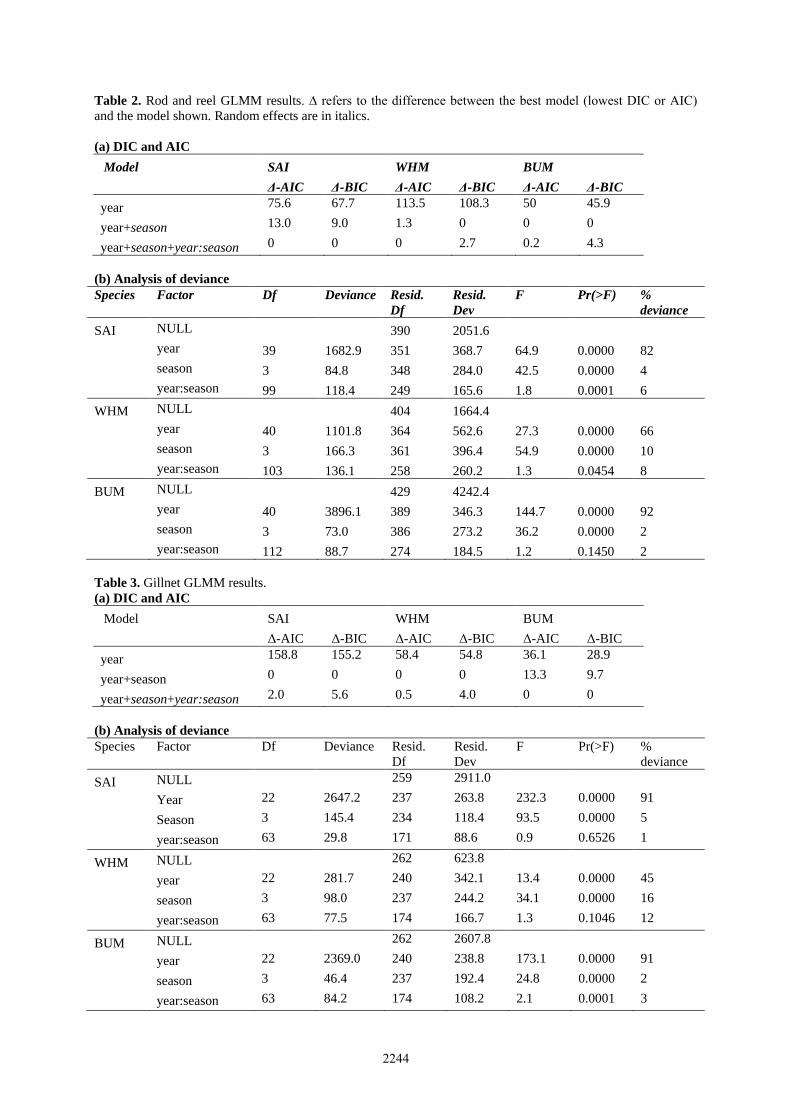
Table 2. Rod and reel GLMM results. ∆ refers to the difference between the best model (lowest DIC or AIC)
and the model shown. Random effects are in italics.
(a) DIC and AIC
Model SAI WHM BUM
Δ-AIC Δ-BIC Δ-AIC Δ-BIC Δ-AIC Δ-BIC
year 75.6 67.7 113.5 108.3 50 45.9
year+season 13.0 9.0 1.3 0 0 0
year+season+year:season 0 0 0 2.7 0.2 4.3
(b) Analysis of deviance
Species
Factor
Df
Deviance
Resid.
Df
Resid.
Dev
F
Pr(>F)
%
deviance
SAI NULL
390 2051.6
year 39 1682.9 351 368.7 64.9 0.0000 82
season 3 84.8 348 284.0 42.5 0.0000 4
year:season 99 118.4 249 165.6 1.8 0.0001 6
WHM NULL
404 1664.4
year 40 1101.8 364 562.6 27.3 0.0000 66
season 3 166.3 361 396.4 54.9 0.0000 10
year:season 103 136.1 258 260.2 1.3 0.0454 8
BUM NULL
429 4242.4
year 40 3896.1 389 346.3 144.7 0.0000 92
season 3 73.0 386 273.2 36.2 0.0000 2
year:season 112 88.7 274 184.5 1.2 0.1450 2
Table 3. Gillnet GLMM results.
(a) DIC and AIC
Model SAI WHM BUM
Δ-AIC Δ-BIC Δ-AIC Δ-BIC Δ-AIC Δ-BIC
year 158.8 155.2 58.4 54.8 36.1 28.9
year+season 0 0 0 0 13.3 9.7
year+season+year:season 2.0 5.6 0.5 4.0 0 0
(b) Analysis of deviance
Species
Factor
Df
Deviance
Resid.
Df
Resid.
Dev
F
Pr(>F)
%
deviance
SAI NULL 259 2911.0
Year 22 2647.2 237 263.8 232.3 0.0000 91
Season 3 145.4 234 118.4 93.5 0.0000 5
year:season 63 29.8 171 88.6 0.9 0.6526 1
WHM NULL 262 623.8
year 22 281.7 240 342.1 13.4 0.0000 45
season 3 98.0 237 244.2 34.1 0.0000 16
year:season 63 77.5 174 166.7 1.3 0.1046 12
BUM NULL 262 2607.8
year 22 2369.0 240 238.8 173.1 0.0000 91
season 3 46.4 237 192.4 24.8 0.0000 2
year:season 63 84.2 174 108.2 2.1 0.0001 3
2244
Table 4. Both datasets combined.
(a) AIC and BIC
Model SAI WHM BUM
Δ-AIC Δ-BIC Δ-AIC Δ-BIC Δ-AIC Δ-BIC
year 142.6 129.2 164.3 153.6 67.4 62.8
year+fishery 144.4 135.4 160.0 153.7 69.1 69.1
year+fishery+season 69.5 65.0 1.7 0 3.5 8.0
year+fishery+season+fishery:season 0 0 0 2.8 0.4 9.4
year+season+year:season 45.1 45.1 3.7 6.4 4.4 13.5
year+season 68.6 59.6 10.2 3.9 0 0
year+season+year:seaon 44.3 39.9 12.0 10.3 1.0 5.5
(b) Analysis of Deviance
Species
Model
Df
Deviance
Resid.
Df
Resid.
Dev
F
Pr(>F)
%
deviance
SAI NULL
648 1393.4
year 50 408.5 598 984.9 7.4 0.0000 29
fishery 1 0.4 597 984.5 0.4 0.5536 0
season 3 157.6 594 826.8 47.8 0.0000 11
year:season 150 330.3 444 496.6 2.0 0.0000 24
fishery:season 3 12.0 441 484.5 3.7 0.0127 1
WHM NULL
665 1478.3
year 50 356.8 615 1121.5 5.4 0.0000 24
fishery 1 10.6 614 1110.9 8.0 0.0048 1
season 3 290.0 611 820.9 73.1 0.0000 20
year:season 150 210.6 461 610.3 1.1 0.3163 14
fishery:season 3 4.9 458 605.4 1.2 0.3009 0
BUM NULL
690 1741.6
year 50 462.6 640 1279.0 5.5 0.0000 27
fishery 1 0.4 639 1278.6 0.3 0.6159 0
season 3 162.9 636 1115.7 32.6 0.0000 9
year:season 150 306.2 486 809.4 1.2 0.0569 18
fishery:season 3 4.2 483 805.2 0.8 0.4721 0
2245

Table 5. Means and standard errors of the indices.
(a) Rod and Reel
Year SAI SE WHM SE BUM SE Year SAI SE WHM SE BUM SE
1961 0.33 0.15 0.33 0.18 0.09 0.04 1981 0.08 0.04 0.63 0.34 0.06 0.02
1962 0.27 0.12 0.46 0.25 0.14 0.05 1982 0.04 0.02 0.67 0.36 0.02 0.01
1963 0.12 0.06 0.26 0.14 0.08 0.03 1983 0.12 0.06 0.34 0.18 0.06 0.02
1964 0.16 0.08 0.36 0.19 0.06 0.02 1984 0.21 0.1 0.29 0.16 0.1 0.04
1965 0.18 0.08 0.23 0.13 0.05 0.02 1985 0.17 0.08 0.32 0.17 0.05 0.02
1966 0.38 0.17 0.28 0.15 0.12 0.05 1986 0.1 0.05 0.14 0.08 0.04 0.02
1967 0.22 0.1 0.23 0.13 0.08 0.03 1987 0.17 0.08 0.16 0.09 0.05 0.02
1968 0.3 0.14 0.23 0.13 0.09 0.03 1988 0.09 0.04 0.16 0.09 0.03 0.01
1969 0.3 0.14 0.18 0.1 0.1 0.04 1989 0.12 0.06 0.12 0.07 0.05 0.02
1970 0.25 0.12 0.11 0.06 0.09 0.04 1991 0.04 0.02 0.05 0.04 0.04 0.02
1971 0.37 0.17 1.04 0.56 0.03 0.02 1992 0.07 0.04 0.2 0.12 0.05 0.02
1972 0.31 0.14 0.52 0.28 0.02 0.01 1993 NA NA 0.06 0.05 0.05 0.03
1973 0.26 0.12 0.9 0.48 0.02 0.01 1994 0.08 0.05 0.08 0.05 0.15 0.07
1974 0.25 0.11 0.23 0.13 0.03 0.01 1995 0.05 0.04 0.16 0.11 0.18 0.08
1975 0.15 0.07 0.34 0.19 0.01 0.01 1996 0.02 0.02 0.02 0.04 0.03 0.01
1976 0.2 0.09 0.54 0.29 0.01 0.01 1997 0.01 0.01 0.02 0.02 0.04 0.02
1977 0.09 0.04 0.3 0.16 0.01 0.01 1998 0.02 0.03 0.03 0.06 0.02 0.02
1978 0.06 0.03 0.16 0.09 0.01 0.01 1999 0.01 0.02 0.04 0.04 0.02 0.02
1979 0.06 0.03 0.27 0.15 0.02 0.01 2000 0.06 0.09 0.01 0.02 0.05 0.03
1980 0.09 0.04 0.52 0.28 0.03 0.01 2001 0.06 0.06 0.2 0.16 0.08 0.04
(b) Gillnet
Year SAI SE WHM SE BUM SE Year SAI SE WHM SE BUM SE
1991 29.45 15.95 3.47 1.74 9.89 4.36 2002 15.98 8.06 2.6 1.25 15.37 6.52
1992 11.8 5.96 0.73 0.35 2.11 0.9 2003 28.46 14.36 3.12 1.5 18.4 7.81
1993 20.72 10.46 0.93 0.45 14.53 6.17 2004 41.23 20.8 4.42 2.12 22.2 9.42
1994 28.91 14.59 6.51 3.12 29.79 12.64 2005 35.1 17.71 3.98 1.91 20.99 8.91
1995 31.38 15.83 3.17 1.52 29.22 12.4 2006 28.23 14.24 3.52 1.69 26.97 11.44
1996 28.75 14.51 0.53 0.26 21.04 8.93 2007 38.09 19.22 5.23 2.51 30.97 13.14
1997 34.98 17.65 0.9 0.44 28.23 11.98 2008 22.78 11.5 3.77 1.81 24.19 10.27
1998 39.5 19.93 2.53 1.22 38.8 16.46 2009 19.85 10.02 2.89 1.39 16.95 7.19
1999 44.56 22.48 4.64 2.23 65.67 27.86 2010 22.07 11.13 1.98 0.95 28.43 12.06
2000 28.17 14.21 3.14 1.51 23.34 9.91 2011 18.36 9.26 1.39 0.67 15.41 6.54
2001 22.61 11.41 1.87 0.9 16.56 7.03 2012 32.8 16.55 3.64 1.75 22.05 9.36
2246

(b) Combined
Year SAI SE WHM SE BUM SE Year SAI SE WHM SE BUM SE
1961 8.18 4.69 3.44 2.01 0.72 0.37 1987 4.17 2.4 1.69 0.99 0.68 0.34
1962 6.7 3.84 5.56 3.24 1.29 0.65 1988 2.12 1.22 1.8 1.05 0.3 0.16
1963 3 1.73 3.06 1.79 0.72 0.36 1989 2.31 1.33 1.36 0.8 0.58 0.3
1964 3.22 1.85 3.69 2.15 0.64 0.33 1990 NA NA NA NA NA NA
1965 3.56 2.05 1.81 1.06 0.46 0.24 1991 0.81 0.42 0.78 0.39 0.38 0.16
1966 7.46 4.28 2.85 1.67 1.6 0.8 1992 0.6 0.29 0.61 0.31 0.27 0.12
1967 4.24 2.43 2.68 1.57 0.71 0.36 1993 0.64 0.34 0.37 0.2 0.5 0.23
1968 7.42 4.25 2.36 1.38 1.17 0.59 1994 1.01 0.5 1.33 0.65 1.23 0.53
1969 5.79 3.32 2.12 1.24 1.34 0.68 1995 0.9 0.45 1.22 0.61 1.36 0.58
1970 6.13 3.52 0.99 0.58 1.19 0.6 1996 0.69 0.34 0.18 0.1 0.47 0.19
1971 9.3 5.34 12.73 7.42 0.21 0.11 1997 0.66 0.33 0.25 0.13 0.68 0.29
1972 7.6 4.36 6.31 3.68 0.21 0.11 1998 0.93 0.48 0.69 0.37 0.76 0.33
1973 6.6 3.79 10.98 6.4 0.11 0.06 1999 0.89 0.45 1.05 0.55 1.2 0.55
1974 6.01 3.45 2.43 1.42 0.2 0.11 2000 0.79 0.41 0.63 0.33 0.72 0.33
1975 3.02 1.74 3.92 2.29 0.04 0.03 2001 0.71 0.36 0.76 0.39 0.69 0.29
1976 3.87 2.22 6.53 3.81 0.05 0.03 2002 0.47 0.25 0.79 0.43 0.5 0.26
1977 1.8 1.04 3.66 2.13 0.06 0.03 2003 0.79 0.42 0.94 0.51 0.6 0.31
1978 1.24 0.72 1.97 1.15 0.09 0.05 2004 1.13 0.6 1.34 0.73 0.73 0.37
1979 1.01 0.58 3.23 1.88 0.17 0.09 2005 0.98 0.51 1.2 0.65 0.69 0.35
1980 1.67 0.96 6.28 3.66 0.18 0.1 2006 0.78 0.41 1.06 0.58 0.88 0.44
1981 1.81 1.04 7.69 4.48 0.73 0.37 2007 1.05 0.55 1.57 0.85 1.01 0.51
1982 0.5 0.29 8.24 4.8 0.12 0.06 2008 0.63 0.33 1.14 0.62 0.79 0.4
1983 2.99 1.72 4.05 2.36 0.82 0.41 2009 0.55 0.29 0.88 0.48 0.56 0.28
1984 5.16 2.96 3.49 2.04 1.29 0.65 2010 0.61 0.32 0.6 0.33 0.93 0.47
1985 4.2 2.41 3.37 1.97 0.62 0.32 2011 0.51 0.27 0.42 0.23 0.5 0.26
1986 2.55 1.46 1.61 0.94 0.36 0.18 2012 0.9 0.48 1.1 0.6 0.72 0.36
2247
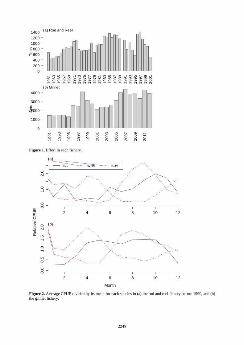
Figure 1. Effort in each fishery.
Figure 2. Average CPUE divided by its mean for each species in (a) the rod and reel fishery before 1990, and (b)
the gillnet fishery.
19
61
19
63
19
65
19
67
19
69
19
71
19
73
19
75
19
77
19
79
19
81
19
83
19
85
19
87
19
89
19
91
19
93
19
95
19
97
19
99
20
01
Tri
ps
0
200
400
600
800
1000
1200
1400(a) Rod and Reel
19
91
19
93
19
95
19
97
19
99
20
01
20
03
20
05
20
07
20
09
20
11
Se
ts
0
1000
2000
3000
4000
(b) Gillnet
2 4 6 8 10 12
0.0
1.0
2.0
SAI WHM BUM
(a)
2 4 6 8 10 12
0.0
0.5
1.0
1.5
2.0
(b)
Month
Re
lative
CP
UE
2248

Figure 3. Histograms of log of CPUE for each species in each fishery.
Figure 4. Rod and Reel model diagnostics.
-5 -3 -1 1
05
15
25
(a) R&R SAI
-5 -3 -1 1 2
05
10
20
(b) R&R WHM
-4 -3 -2 -1
020
40
60
(c) R&R BUM
-2 0 2 4
010
20
30
40
(d) Gillnet SAI
-4 -2 0 2
05
10
15
20
(e) Gillnet WHM
-4 -2 0 2 4
020
40
60
(f) Gillnet BUM
Log(CPUE+0.01)
Co
un
t
-4 -3 -2 -1 0
-20
2
Predicted values
Resid
uals
(a) SAI
-3 -2 -1 0 1 2 3
-20
2
Theoretical Quantiles
Sam
ple
Quantil
es
-4 -3 -2 -1 0 1
-3-1
1
Predicted values
Resid
uals
(b) WHM
-3 -2 -1 0 1 2 3
-3-1
1
Theoretical Quantiles
Sam
ple
Quantil
es
-4.5 -3.5 -2.5 -1.5
-20
Predicted values
Resid
uals
(c) BUM
-3 -2 -1 0 1 2 3
-20
Theoretical Quantiles
Sam
ple
Quantil
es
2249

Figure 5. Rod and Reel fitted values.
1960 1970 1980 1990 2000
0.0
0.4
0.8
1.2 (a) SAI
Index & 95% CIGaertner & AlioRaw meanLognormal mean
1960 1970 1980 1990 2000
0.0
1.0
2.0
(b) WHM
1960 1970 1980 1990 2000
0.0
0.2
(c) BUM
Year
CP
UE
2250
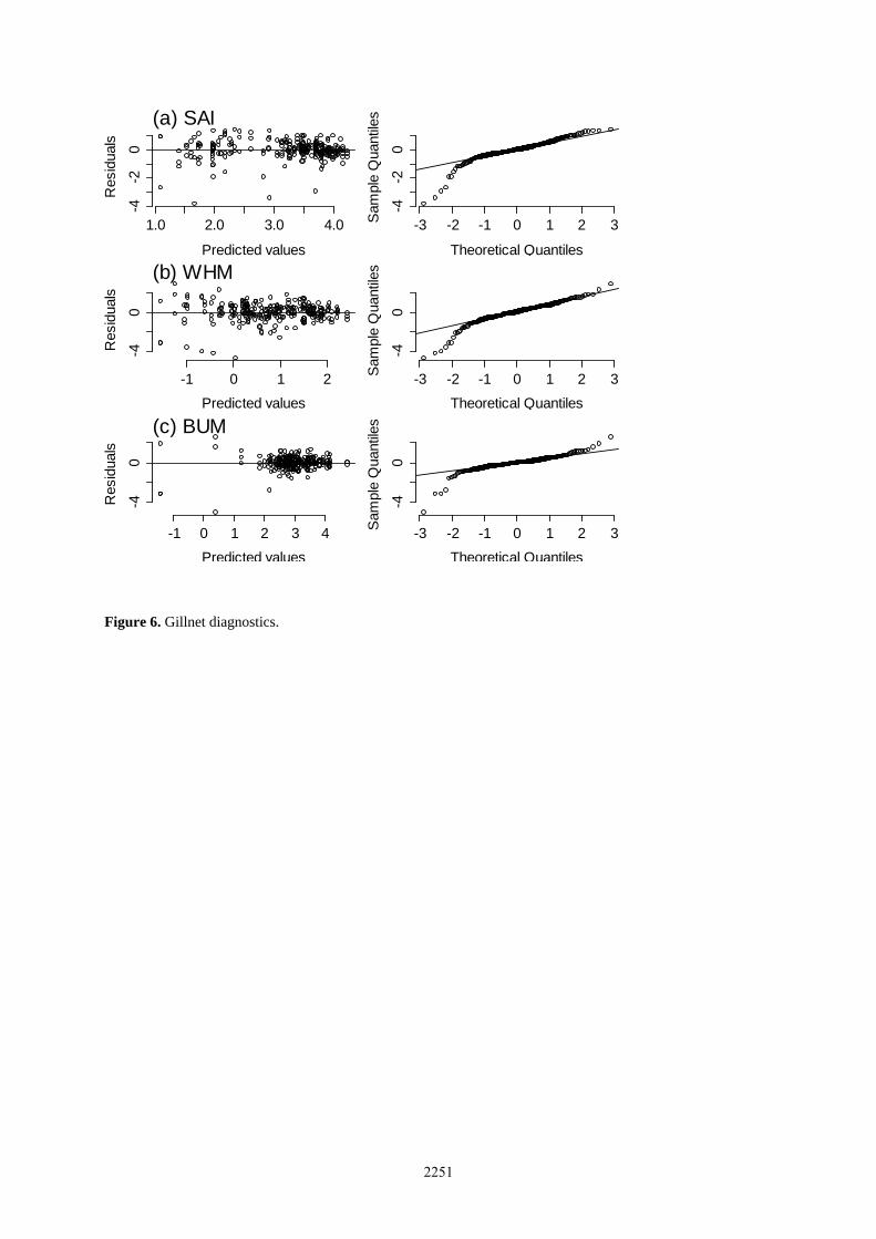
Figure 6. Gillnet diagnostics.
1.0 2.0 3.0 4.0
-4-2
0
Predicted values
Resid
uals
(a) SAI
-3 -2 -1 0 1 2 3
-4-2
0
Theoretical Quantiles
Sam
ple
Quantil
es
-1 0 1 2
-40
Predicted values
Resid
uals
(b) WHM
-3 -2 -1 0 1 2 3-4
0Theoretical Quantiles
Sam
ple
Quantil
es
-1 0 1 2 3 4
-40
Predicted values
Resid
uals
(c) BUM
-3 -2 -1 0 1 2 3
-40
Theoretical Quantiles
Sam
ple
Quantil
es
2251

Figure 7. Gillnet fitted values.
1995 2000 2005 2010
020
60
100 (a) SAI
1995 2000 2005 2010
04
812
(b) WHM
1995 2000 2005 2010
040
80
120
(c) BUM
Index & 95% CI
Arocha et al.
Raw mean
Lognormal mean
Year
CP
UE
2252

Figure 8. Diagnostics for the model with both datasets.
-2 -1 0 1 2
-40
Predicted values
Resid
uals
(a) SAI
-3 -2 -1 0 1 2 3
-40
Theoretical Quantiles
Sam
ple
Quantil
es
-3 -2 -1 0 1 2
-40
Predicted values
Resid
uals
(b) WHM
-3 -2 -1 0 1 2 3
-40
Theoretical Quantiles
Sam
ple
Quantil
es
-3 -2 -1 0 1
-40
Predicted values
Resid
uals
(c) BUM
-3 -2 -1 0 1 2 3
-40
Theoretical Quantiles
Sam
ple
Quantil
es
2253

Figure 9. Fitted values for both datasets together.
1960 1970 1980 1990 2000 2010
010
20
(a) SAI
1960 1970 1980 1990 2000 2010
010
25
(b) WHM
1960 1970 1980 1990 2000 2010
01
23
(c) BUM
Year
CP
UE
2254

Figure 10. Fitted values for the two series separately.
1960 1970 1980 1990 2000 2010
05
10
15
(a) SAI
Rod and Reel
Gillnet
1960 1970 1980 1990 2000 2010
05
15
25
(b) WHM
1960 1970 1980 1990 2000 2010
01
23
45
(c) BUM
Year
CP
UE
2255