STANDARD NORMAL PROBABILITIES - rd.springer.com978-1-4757-2926-9/1.pdf · Table I: STANDARD NORMAL...
37
Table I: STANDARD NORMAL PROBABILITIES The table reports the area to the left of the value z under the standard nor- mal curve. - 4.0 - 2.0 0.0 2.0 4.0 z 0 1 2 3 _4 5 - 6 7 8 9 -3.4 .0003 .0003 .0003 .0003 .0003 .0003 .0003 .0003 .0003 .0002 -3.3 .0005 .0005 .0005 .0004 .0004 .0004 .0004 .0004 .0004 .0004 -3 .2 .0007 .0007 .0006 .0006 .0006 .0006 .0006 .0005 .0005 .0005 -3 .1 .0010 .0009 .0009 .0009 .0008 .0008 .0008 .0008 .0007 .0007 -3 .0 .0014 .0013 .0013 .0012 .0012 .0011 .0011 .0011 .0010 .0010 -2.9 .0019 .0018 .0018 .0017 .0016 .0016 .0015 .0015 .0014 .0014 -2.8 .0026 .0025 .0024 .0023 .0023 .0022 .0021 .0021 .0020 .0019 -2.7 .0035 .0034 .0033 .0032 .0031 .0030 .0029 .0028 .0027 .0026 -2 .6 .0047 .0045 .0044 .0043 .0041 .0040 .0039 .0038 .0037 .0036 -2.5 .0062 .0060 .0059 .0057 .0055 .0054 .0052 .0051 .0049 .0048 -2.4 .0082 .0080 .0078 .0075 .0073 .0071 .0069 .0068 .0066 .0064 -2 .3 .0107 .0104 .0102 .0099 .0096 .0094 .0091 .0089 .0087 .0084 447
Transcript of STANDARD NORMAL PROBABILITIES - rd.springer.com978-1-4757-2926-9/1.pdf · Table I: STANDARD NORMAL...

Table I:
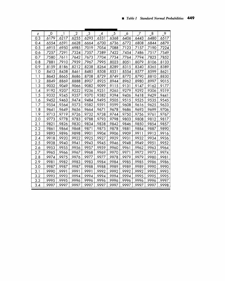
STANDARD NORMAL PROBABILITIES
The table reports the area to the left of the value z under the standard normal curve.
- 4.0 - 2.0 0.0 2.0 4.0
z 0 1 2 3 _4 5 -6 7 8 9 -3.4 .0003 .0003 .0003 .0003 .0003 .0003 .0003 .0003 .0003 .0002 -3.3 .0005 .0005 .0005 .0004 .0004 .0004 .0004 .0004 .0004 .0004 -3.2 .0007 .0007 .0006 .0006 .0006 .0006 .0006 .0005 .0005 .0005 -3.1 .0010 .0009 .0009 .0009 .0008 .0008 .0008 .0008 .0007 .0007 -3 .0 .0014 .0013 .0013 .0012 .0012 .0011 .0011 .0011 .0010 .0010 -2.9 .0019 .0018 .0018 .0017 .0016 .0016 .0015 .0015 .0014 .0014 -2.8 .0026 .0025 .0024 .0023 .0023 .0022 .0021 .0021 .0020 .0019 -2.7 .0035 .0034 .0033 .0032 .0031 .0030 .0029 .0028 .0027 .0026 -2 .6 .0047 .0045 .0044 .0043 .0041 .0040 .0039 .0038 .0037 .0036 -2.5 .0062 .0060 .0059 .0057 .0055 .0054 .0052 .0051 .0049 .0048 -2.4 .0082 .0080 .0078 .0075 .0073 .0071 .0069 .0068 .0066 .0064 -2.3 .0107 .0104 .0102 .0099 .0096 .0094 .0091 .0089 .0087 .0084
447

448 • Table I Standard Nonnal Probabilities
z 0 1 2 3 4 5 6 7 8 9 - 2.2 .0139 .0136 .0132 .0129 .0125 .0122 .0119 .0116 .0113 .0110 -2.1 .0179 .0174 .0170 .0166 .0162 .0158 .0154 .0150 .0146 .0143 -2 .0 .0228 .0222 .0217 .0212 .0207 .0202 .0197 .0192 .0188 .0183 -1.9 .0287 .0281 .0274 .0268 .0262 .0256 .0250 .0244 .0239 .0233 -1.8 .0359 .0351 .0344 .0336 .0329 .0322 .0314 .0307 .0301 .0294 -1.7 .0446 .0436 .0427 .0418 .0409 .0401 .0392 .0384 .0375 .0367 -1.6 .0548 .0537 .0526 .0516 .0505 .0495 .0485 .0475 .0465 .0455 -1.5 .0668 .0655 .0643 .0630 .0618 .0606 .0594 .0582 .0571 .0559 -1.4 .0808 .0793 .0778 .0764 .0749 .0735 .0721 .0708 .0694 .0681 -1.3 .0968 .0951 .0934 .0918 .0901 .0885 .0869 .0853 .0838 .0823 -1.2 .1151 .1131 .1112 .1093 .1075 .1057 .1038 .1020 .1003 .0985 -1.1 .1357 .1335 .1314 .1292 .1271 .1251 .1230 .1210 .1190 .1170 -1.0 .1587 .1562 .1539 .1515 .1492 .1469 .1446 .1423 .1401 .1379 -0.9 .1841 .1814 .1788 .1762 .1736 .1711 .1685 .1660 .1635 .1611 -0.8 .2119 .2090 .2061 .2033 .2005 .1977 .1949 .1922 .1894 .1867 -0.7 .2420 .2389 .2358 .2327 .2297 .2266 .2236 .2207 .2177 .2148 -0.6 .2743 .2709 .2676 .2643 .2611 .2578 .2546 .2514 .2483 .2451 -0.5 .3085 .3050 .3015 .2981 .2946 .2912 .2877 .2843 .2810 .2776 -0.4 .3446 .3409 .3372 .3336 .3300 .3264 .3228 .3192 .3156 .3121 -0.3 .3821 .3783 .3745 .3707 .3669 .3632 .3594 .3557 .3520 .3483 -0.2 .4207 .4168 .4129 .4090 .4052 .4013 .3974 .3936 .3897 .3859 -0.1 .4602 .4562 .4522 .4483 .4443 .4404 .4364 .4325 .4286 .4247 -0.0 .5000 .4960 .4920 .4880 .4840 .4801 .4761 .4721 .4681 .4641
The table reports the area to the left of the value z under the standard normal curve.
- 4.0 -2.0 0.0 2.0 4.0
z 0 1 2 3 4 5 6 7 8 9 -0 .0 .5000 .5040 .5080 .5120 .5160 .5199 .5239 .5279 .5319 .5359 0.1 .5398 .5438 .5478 .5517 .5557 .5596 .5636 .5675 .5714 .5753 0 .2 .5793 .5832 .5871 .5910 .5948 .5987 .6026 .6064 .6103 .6141
• Table I Standard N()f71I(lI Probabilities 449
z 0 -1 2 3 4 _5 6 7 8 9 0.3 .6179 .6217 .6255 .6293 .6331 .6368 .6406 .6443 .6480 .6517 0.4 .6554 .6591 .6628 .6664 .6700 .6736 .6772 .6808 .6844 .6879 0.5 .6915 .6950 .6985 .7019 .7054 .7088 .7123 .7157 .7190 .7224 0.6 .7257 .7291 .7324 .7357 .7389 .7422 .7454 .7486 .7517 .7549 0.7 .7580 .7611 .7642 .7673 .7704 .7734 .7764 .7794 .7823 .7852 0.8 .7881 .7910 .7939 .7967 .7995 .8023 .8051 .8079 .8106 .8133 0.9 .8159 .8186 .8212 .8238 .8264 .8289 .8315 .8340 .8365 .8389 1.0 .8413 .8438 .8461 .8485 .8508 .8531 .8554 .8577 .8599 .8621 1.1 .8643 .8665 .8686 .8708 .8729 .8749 .8770 .8790 .8810 .8830 1.2 .8849 .8869 .8888 .8907 .8925 .8944 .8962 .8980 .8997 .9015 1.3 .9032 .9049 .9066 .9082 .9099 .9115 .9131 .9147 .9162 .9177 1.4 .9192 .9207 .9222 .9236 .9251 .9265 .9279 .9292 .9306 .9319 1.5 .9332 .9345 .9357 .9370 .9382 .9394 .9406 .9418 .9429 .9441 1.6 .9452 .9463 .9474 .9484 .9495 .9505 .9515 .9525 .9535 .9545 1.7 .9554 .9564 .9573 .9582 .9591 .9599 .9608 .9616 .9625 .9633 1.8 .9641 .9649 .9656 .9664 .9671 .9678 .9686 .9693 .9699 .9706 1.9 .9713 .9719 .9726 .9732 .9738 .9744 .9750 .9756 .9761 .9767 2.0 .9773 .9778 .9783 .9788 .9793 .9798 .9803 .9808 .9812 .9817 2.1 .9821 .9826 .9830 .9834 .9838 .9842 .9846 .9850 .9854 .9857 2.2 .9861 .9864 .9868 .9871 .9875 .9878 .9881 .9884 .9887 .9890 2.3 .9893 .9896 .9898 .9901 .9904 .9906 .9909 .9911 .9913 .9916 2.4 .9918 .9920 .9922 .9925 .9927 .9929 .9931 .9932 .9934 .9936 2.5 .9938 .9940 .9941 .9943 .9945 .9946 .9948 .9949 .9951 .9952 2.6 .9953 .9955 .9956 .9957 .9959 .9960 .9961 .9962 .9963 .9964 2.7 .9965 .9966 .9967 .9968 .9969 .9970 .9971 .9972 .9973 .9974 2.8 .9974 .9975 .9976 .9977 .9977 .9978 .9979 .9979 .9980 .9981 2.9 .9981 .9982 .9983 .9983 .9984 .9984 .9985 .9985 .9986 .9986 3.0 .9987 .9987 .9987 .9988 .9988 .9989 .9989 .9989 .9990 .9990 3.1 .9990 .9991 .9991 .9991 .9992 .9992 .9992 .9992 .9993 .9993 3.2 .9993 .9993 .9994 .9994 .9994 .9994 .9994 .9995 .9995 .9995 3.3 .9995 .9995 .9996 .9996 .9996 .9996 .9996 .9996 .9996 .9997 3.4 .9997 .9997 .9997 .9997 .9997 .9997 .9997 .9997 .9997 .9998

Table II:
,-DISTRIBUTION CRITICAL VALUES
The table reports the critical value for which the area to the right is as indicated.
- 5.0 -2.5 0.0 2.5 5.0
Area to ri!=lht 0.2 0.1 0.05 0.025 0.01 0.005 0.001 0.0005 Conf. level 60% 80% 90% 95% 98% 99% 99.80% 99.90%
dJ 1 1.376 3.078 6.314 12.706 31.821 63.657 318.317 636.607 2 1.061 1.886 2.920 4.303 6.965 9.925 22.327 31.598 3 0.978 1.638 2.353 3.182 4.541 5.841 10.215 12.924 4 0.941 1.533 2.132 2.776 3.747 4.604 7.173 8.610 5 0 .920 1.476 2.015 2.571 3.365 4.032 5.893 6.869 6 0.906 1.440 1.943 2.447 3.143 3.708 5.208 5.959 7 0.896 1.415 1.895 2.365 2.998 3.500 4.785 5.408 8 0.889 1.397 1.860 2.306 2.897 3.355 4.501 5.041 9 0.883 1.383 1.833 2.262 2.821 3.250 4.297 4.781 10 0.879 1.372 1.812 2.228 2.764 3.169 4.144 4.587
451

452 • Table II t-Distribution Critical Values
Area to riQht 0.2 0.1 0.05 0.025 0.01 0.005 0.001 0.0005 Conf. level 60% 80% 90% 95% 98% 99% 99.80% 99.90%
dJ. 11 0.876 1.363 1.796 2.201 2.718 3.106 4.025 4.437 12 0.873 1.356 1.782 2.179 2.681 3.055 3.930 4.318 13 0.870 1.350 1.771 2.160 2.650 3.012 3.852 4.221 14 0.868 1.345 1.761 2.145 2.625 2.977 3.787 4.140 15 0.866 1.341 1.753 2.131 2.602 2.947 3.733 4.073 16 0.865 1.337 1.746 2.120 2.583 2.921 3.686 4.015 17 0.863 1.333 1.740 2.110 2.567 2.898 3.646 3.965 18 0.862 1.330 1.734 2.101 2.552 2.878 3.611 3.922 19 0.861 1.328 1.729 2.093 2.539 2.861 3.579 3.883 20 0.860 1.325 1.725 2.086 2.528 2.845 3.552 3.850 21 0.859 1.323 1.721 2.080 2.518 2.831 3.527 3.819 22 0.858 1.321 1.717 2.074 2.508 2.819 3.505 3.792 23 0.858 1.319 1.714 2.069 2.500 2.807 3.485 3.768 24 0.857 1.318 1.711 2.064 2.492 2.797 3.467 3.745 25 0.856 1.316 1.708 2.060 2.485 2.787 3.450 3.725 26 0.856 1.315 1.706 2.056 2.479 2.779 3.435 3.707 27 0.855 1.314 1.703 2.052 2.473 2.771 3.421 3.690 28 0.855 1.313 1.701 2.048 2.467 2.763 3.408 3.674 29 0.854 1.311 1.699 2.045 2.462 2.756 3.396 3.659 30 0.854 1.310 1.697 2.042 2.457 2.750 3.385 3.646 40 0.851 1.303 1.684 2.021 2.423 2.704 3.307 3.551 50 0.849 1.299 1.676 2.009 2.403 2.678 3.261 3.496 60 0.848 1.296 1.671 2.000 2.390 2.660 3.232 3.460 80 0.846 1.292 1.664 1.990 2.374 2.639 3.195 3.416 100 0.845 1.290 1.660 1.984 2.364 2.626 3.174 3.391 500 0.842 1.283 1.648 1.965 2.334 2.586 3.107 3.310
Infinity 0.842 1.282 1.645 1.960 2.326 2.576 3.090 3.291
Appendix A:
OVERVIEW OF MINITAB®
Starting Minitab:
To launch Minitab, click your (left) mouse button two times quickly while pointing to the Minitab icon or the Minitab Student icon: ~~
Once in Minitab:
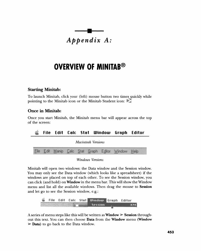
Once you start Minitab, the Minitab menu bar will appear across the top of the screen:
, File Edit Calc Stat Window Graph Editor
Macintosh Versions
Manip ~alc ~t Window Help
Windows Versions
Minitab will open two windows: the Data window and the Session window. You may only see the Data window (which looks like a spreadsheet) if the windows are placed on top of each other. To see the Session window, you can click (and hold) on Window in the menu bar. This will show the Window menu and list all the available windows. Then drag the mouse to Session and let go to see the Session window, e.g.:
A series of menu steps like this will be written as Window:> Session throughout this text. You can then choose Data from the Window menu (Window :> Data) to go back to the Data window.
453

454 • Appendix A Overview of Minitab
The Data window is used for entering, viewing, and editing data. Each column contains data for a different variable. The rows contain the observations for different cases:
10 ------ 1];; Data
C1 C2 Cl C2 C3 C4 I , ,- I 1
I 2
Macintosh Versions Windows Versions
The Session window is used for entering Minitab commands that tell the program what to do:
Ib"kshItt Sill : 3500 ct lls me > I
~II
SHllo.
Macintosh Versions
Vark.heel .... )500 0.11.
1m)
Windows Versions
You should always click in the Session window to highlight it before you start entering commands. In the Windows Professional version you need to select Editor> Enable Command Language from the menu before you will see the MTB> prompt. Minitab commands can also be given using the menus across the top of the screen.
You can resize and move these windows for more convenient viewin~: Click on the box in the lower right comer of the window (e.g. ~ or Ill) and drag to resize. You can also click and hold the mouse button down on the top bar of the window and drag the mouse to move the window.
Entering Data into Minitab:
To type data into the Minitab worksheet directly, activate the Data window and type each data value into a different cell, hitting Return, Enter, Tab, or arrows to move from cell to cell. Remember that each column contains data for a different variable.

• Appendix A Overoiew of Minitab 455
In the Professional Versions and the Windows Student Version, the arrow in the upper left comer of the Data window determines the direction in which the Minitab cursor moves when you press Enter/Return.
(1 (1 ............................. .............................
1 1 ..................................................... . ................................................... .
Clicking the mouse on this arrow changes its direction. If the arrow is pointing down, hitting Return/Enter moves you to the next row in the same column. If the arrow points to the right, hitting Return/Enter moves you to the next column in the same row.
Opening an Existing Minitab Worksheet:
The data sets in this book are available in Minitab worksheets. You can open such a file by choosing File :;0.. Open Worksheet from the menu bar. You will then see a list of saved worksheets (with the . m tw extension).
Note: In the Windows Student version, you will be asked to select a file type. In this book, all files will be "Minitab Worksheets," so just click on the SELECT FILE button.
Once you find the file you want, you can click on the file name once to highlight it, and then click on the OK/OPEN button, or you can double click on the file name. Check that the data now appear in the Data window.
Note: In this book, we assume the Minitab worksheets are stored in the default Minitab Data folder. If the data are stored elsewhere, e.g. on your disk, you will need to change folders. See Activity 1-4 for an example.
Using Minitab Commands:
Commands for Minitab are either typed in at the MTB> prompt in the Session window or by using the menu bar (notice that after selecting a command with the menus, the equivalent session commands appear in the Session window). In this book these commands will appear in this font. As you use Minitab you will find some situations for which typing the command directly is easier and others for which using the menu bar is easier. Each command produces output or updates the Data window. Output appears either in the Session window or in a special graphics window.

456 • Appendix A Overview of Minitab
Sub commands:
You will occasionally want to specify a subcommand to a command in the Session window. Minitab uses a semicolon to signify that the next line should be a subcommand. For example:
MTB> hist el; SUBC>
The prompt changes to SUBC> because Minitab is now expecting a subcommand. You can continue to issue subcommands by ending each line with a semicolon. To indicate that you are finished with subcommands, type a period at the end of the last subcommand. For example:
MTB> hist el; SUBC> iner 5; SUBC> by e2.
Minitab will produce the histogram and then change back to the MTB> prompt, awaiting your next command.
Reverting a Minitab Worksheet:
If you make changes to a Minitab worksheet but then want to return to the last saved version of the worksheet, choose File» Revert Worksheet from the menu bar. In the Windows Professional version choose File » Restart Minitab, clicking on NO when asked if you want to save changes to the data file.
Opening an Empty Minitab Worksheet:
If you have been working in Minitab and want to change to a new (empty) worksheet, choose File» New Worksheet from the menu bar. Minitab will ask if you want to save any changes you made to the previous worksheet.
Deleting Data:
To delete a cell entry, click the mouse on the undesired value and press the delete/backspace key. When you hit Return/Enter, the value will be replaced by a * which Minitab uses to represent a missing observation.
To delete an entire row, click the mouse in the undesired row in the Data window and choose Editor» Delete Row (Macintosh Student, making sure you choose the Editor, not the Edit, menu) or Manip » Delete Row from the menu bar (Other versions). In the latter case, specifY the row number(s) in the first box and which column(s) you want the row values to be deleted

• Appendix A Overoiew of Minitab 457
from in the second box. This allows you to delete rows from a subset of columns, e.g. rows 1, 2 and 5 from Cl. Alternatively, you can also type:
MTB> dele 1:2 5 c1
at the Minitab prompt in any version of the Minitab program.
To delete an entire Minitab column, e.g. Cl, type:
MTB> erase c1
at the Minitab prompt or choose Manip );;>- Erase Variables III the Professional versions and Windows Student versions.
Pending Cell Change/Dimmed Menu Items:
To move from cell to cell in the Data window, you can use the arrow keys, the tab key, or hit return/enter. You must finish putting data in a cell (complete the cell) before you can execute a command. When you have not completed a cell, many menu items will be dimmed so that you can not select them. If you then try to execute a command in the Session window, Minitab will tell you it cannot execute the command until you accept the pending cell change. To fix this problem, go back to the Data window and press enter, return, tab, or an arrow key. The highlighted cell then fills in, enabling you to issue a command. Thus, whenever Minitab will not accept a command, make sure that the current cell in the Data window is filled in. Similarly, if you haven't finished executing a command in the Session window, Minitab will not let you select items from the menus.
Alpha Columns:
Entering any letters into a column converts it to an alpha column, preventing you from performing any mathematical operations on that column. If you accidentally type a letter and notice your mistake before you complete the cell, use the delete key or select Edit );;>- Undo Cell Changes (Macintosh Student) or Edit );;>- Undo Change Within a Cell (Macintosh Professional, Windows Student). An alternative is to use the erase command, which deletes the entire column and removes the alpha column designation. You can then reenter the numeric data. In the Windows Professional version you can choose Manip );;>- Change Data Type as well.
Saving Your Worksheet:
When you are entering your own data, you should periodically save the worksheet by choosing File);;>- Save Worksheet. If you have not already done so, Minitab asks you to name the worksheet and then creates a file with that name and the extension . mtw. You should save the worksheet onto your

458 • Appendix A Overview of Minitab
disk directly. See Activity 1-3 for an example. Use File >- Save Worksheet As to save an existing worksheet under a new name. This is useful for creating your own copies of the textbook worksheets before you make changes to them.
Saving Minitab Output:
There are three main ways to save Minitab output:
a) Recording Sessions: (Macintosh versions, Windows Student version) You may occasionally want to keep a record of the Minitab output and the commands you have used. Initiate this process by selecting File >- Other Files >- Start Recording Session from the menu bar. You should always remember to do this before you start working. Click on the SELECT FILE button in the next window or press Return/Enter. In the next window, enter a name for the file in the box under "Record Session as" or "File name". You should always save these files to your disk. Click on the SAVE/OK button and Minitab creates a file with this name and the extension .lis. You can close this . 1 i s file by either exiting Minitab or choosing File >- Other FIle >- Stop Recording Session. If you then choose Start Recording Session again later, and use the same name, the new output will be appended to the file. The . 1 i s file can be opened by most word processing applications so that you may edit your output. Open the . 1 i s file from within the word processing application; do not try to double click on the file icon.
b) Saving the Session Wmdow: If you forget to record the session you can still save all of the output contained in the Session window. Make sure the Session window is highlighted and choose File >- Save Wmdow As. You should change folders, name the file, and save it to your disk. This file can then be opened by any word processing program.
c) Cutting and Pasting Minitab Output: If you have both Minitab and a word processing program open at the same time, you can select portions of the Minitab output by holding the mouse button down and dragging over that section. Once the region you desire is selected, choose Edit >- Copy or type ~:C/ ctrl C to copy that text. Move to the word processing document and then select Edit >- Paste or type ~ V / ctrl V to paste the section where you want it in your word processing document.
Saving High-Resolution Graphs:
When Minitab creates a high-resolution graph, the graph appears in a new window instead of in the Session window. To save this graphics window, make sure the window is active and choose File >- Save Wmdow As. You can then name this graphics file and save it to your disk. The Windows ver-

• Appendix A Overoiew of Minitab 459
sions will add the . mgf extension. This graph can then be imported into a word processing program. Alte"rnatively, you can copy the graphics window (Edit >- Copy Graph) and then paste the graph into a word processing file.
Printing High-Resolution Graphs:
If you want to print a high-resolution graph directly, make sure the graphics window is highlighted and choose File >- Print Wmdow. Click on OK in the Print Window screen. The graph can then be labeled and included with your work. Note: It is often more economical to import the graph into a word processing file first and then add text and comments around the graph. In many applications, you can trim the excess white space surrounding these graphs by clicking on the graph once and then holding the shift key down while you use the mouse to move the edge of the picture inward.
When you are done with the graphics window, you can click in the box in the upper left corner (Macintosh) or upper right corner (left square, Windows) of the window to close it. Notice that you can get this window back by selecting its name from the bottom of the Wmdow submenu. To get rid of the window permanently, choose Wmdow >- Manage Graph (Professional Windows) or Wmdow >- Discard Graph (Other versions). In the Windows versions, you can also click in the right square (with the X) in the upper right corner.
Using Macros:
You will occasionally be asked to execute Minitab macros, which are files that contain a sequence of Minitab commands. To run a macro, choose File >- Other Files >- Execute Macro (Macintosh Student) or File >- Other Files >- Run an Exec (Other versions) from the menu bar.
Minitab will first ask you how many times you want to run the macro. You should usually run the macro once to make sure that it works and then as many more times as is required for the activity. Next you have to tell Minitab which macro to execute. This book assumes that macros are stored in the default Minitab Macros folder and always end in the extension .mtb. You can view the commands issued by the macro by opening up this . mtb file in any word processing application.
Printing Data:
You cannot print data directly from the Data window. To print some or all of the data, use the print command, e.g.:
MTB> print cl-c5
which will type the data in columns 1-5 into the Session window where it

460 • Appendix A Overview of Minitab
can be recorded, saved, or printed directly. In the Macintosh versions, you can use the mouse to select the data and then choose File» Print Selection from the menu bar.
Getting Minitab Help:
Minitab has extensive on-line help documentation. To view the help files, you can either choose Help from the menu (Macintosh) or choose Help from the Minitab menu bar (Windows) or type help at the MTB> prompt in the Session window. You can also type help followed by a command to find help on a specific command. For example, typing
MTB> help commands
displays a table of contents for all possible Minitab commands. Double clicking on one of these commands will give you an information window for that command and list any potential subcommands.
Quitting Minitab:
When you are done using Minitab, click on File in the menu bar and drag the mouse to Quit/Exit or hit ~:Q (Macintosh) or Alt-F-X (Windows) to quit the program.
If you have been using a Minitab worksheet created for class use, you should NOT save your changes to the worksheet. You should either save the changes under a different worksheet name on your disk (File» Save Worksheet As) or simply exit Minitab and answer NO when asked if you want to save changes.
Please note that closing all windows is not equivalent to exiting the Minitab program.

Appendix B:
STUDENT GLOSSARY
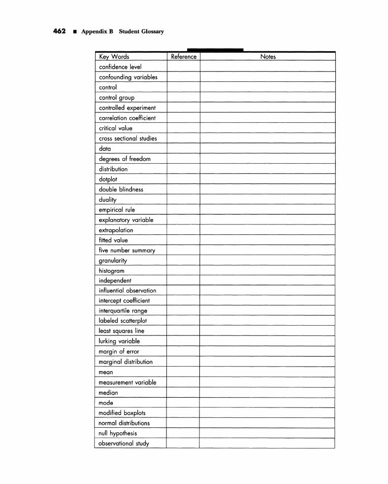
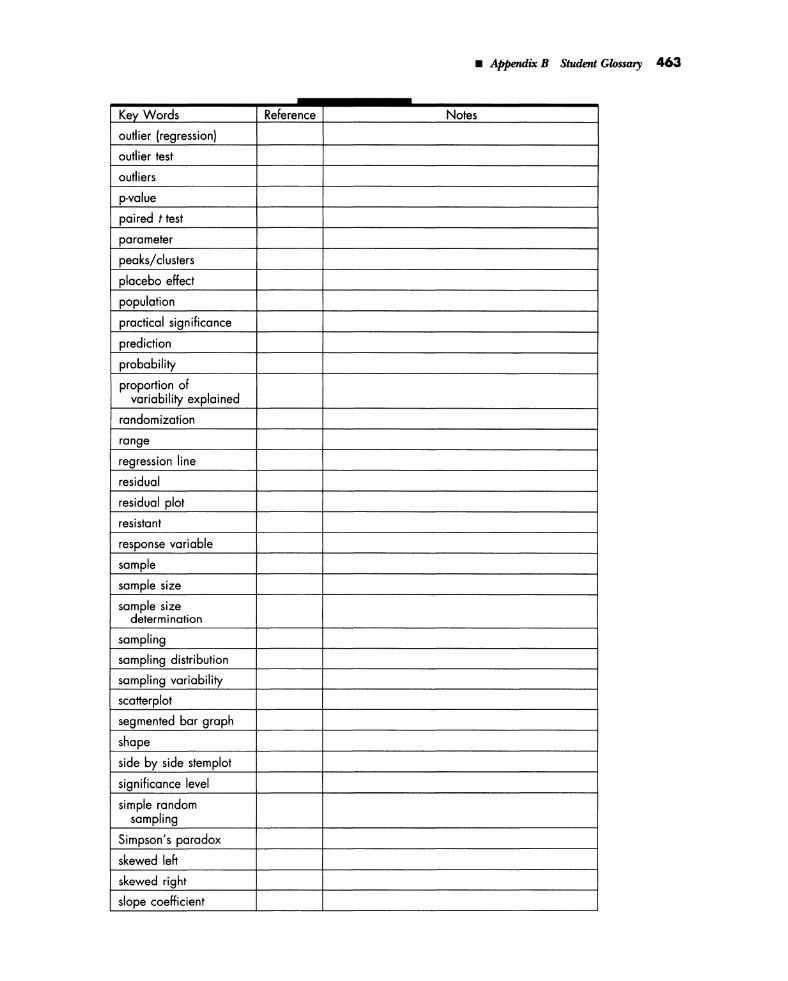
This "do-it-yourself" glossary is meant to provide you with an opportunity to organize definitions of key terms in one location. The following key terms are all marked in the text in bold. You should feel free to write definitions or properties of these terms in this glossary as you encounter them in the text. You can also record several topic numbers or activity numbers or page numbers for each key word, as each term may appear in more than one activity throughout the text.
Key Words Reference Notes 45° line
alternative hypothesis
association
bar graph
biased sampling
binary variable
boxplot
case control studies
categorical variable
causation
center
central limit theorem
clinical trials
cohort studies
comparison
conditional distribution
confidence
confidence interval
461
462 • Appendix B Student Glossary
Key Words Reference Notes
confidence level
confounding variables
control
control group
controlled experiment
correlation coefficient
critical value
cross sectional studies
data
degrees of freedom
distribution
dotplot
double blindness
duality
empirical rule
explanatory variable
extrapolation
fitted value
five number summary
granularity
histogram
independent
influential observation
intercept coefficient
interquartile range
labeled scatterplot
least squares line
lurking variable
margin of error
marginal distribution
mean
measurement variable
median
mode
modified boxplots
normal distributions
null hypothesis
observational study
• Appendix B Student Glossary 463
Key Words Reference Notes
ourlier (regression)
outlier test
outliers
p-value
paired t test
parameter
peaks/clusters
placebo effect
population
practical significance
prediction
probability
proportion of variability explained
randomization
range
regression line
residual
residual plot
resistant
response variable
sample
sample size
sample size determ i nation
sampling
sampling distribution
sampling variability
scatterplot
segmented bar graph
shape
side by side stem plot
significance level
simple random sampling
Simpson's paradox
skewed left
skewed right
slope coefficient

464 • Appendix B Student Glossary
Key Words Reference Notes
standard deviation
standard normal distribution
standard normal table
standardization
standardized score
statistic
statistical significance
statistical tendency
stemplot
symmetric
t distribution
t interval
t test
table of random digits
tally
test decision
test of significance
test statistic
transformation
two sample t interval
two sample t test
two sample z interval
two sample z test
two sided test
two-way table
variability
variable
z-score

Appendix C:
LISTINGS OF HYPOTHETICAL DATA SETS
Many of the hypothetical data sets used in the text present graphical displays without listing the actual data values. These values are necessary in some calculations, so they are presented below.
Activities 3-1: Hypothetical Exam Scores; 4-3: Properties of Averages; 5-2: Properties of Measures of Spread (HYPOFEAT.MlW)
Class A Class B Class C Class D Class E Class F Class G Class H Class I 89 71 66 69 71 56 37 33 37 73 71 54 72 71 61 58 40 57 73 52 55 70 52 67 56 38 55 75 74 61 71 74 57 47 52 16 88 74 59 72 74 81 45 76 51 95 72 62 74 72 68 40 62 60 81 69 59 72 69 75 42 38 27 73 75 56 68 75 72 63 73 65 76 63 57 79 63 91 51 88 66 73 69 58 70 69 71 60 54 53 75 65 50 70 65 66 66 59 52 80 65 66 71 65 96 32 39 67 81 63 59 72 63 83 79 33 42 92 72 50 70 72 62 47 57 59 98 75 61 72 75 78 73 51 47 85 60 66 71 60 71 29 46 65 70 65 47 68 65 61 64 41 51 77 73 46 73 73 68 49 54 47 85 68 60 72 68 72 51 51 33 83 66 62 70 66 72 63 43 56 88 68 63 72 68 60 62 62 25
465

466 • Appendix C Listings of Hypothetical Data Sets
Class A Class B Class C Class D Class E Class F Class G Class H Class I 74 78 60 70 78 64 44 45 63 84 67 77 66 67 71 30 51 66 90 77 67 72 77 58 43 51 51 81 63 55 73 63 72 57 49 38 81 70 51 69 70 50 70 68 57 83 63 65 66 63 70 33 39 22 68 66 60 72 66 82 58 57 31 91 59 55 67 59 73 61 59 46 82 61 72 68 61 72 51 49 52 70 74 63 71 74 65 65 84 37 78 75 68 72 75 90 29 37 45 77 72 65 72 72 55 76 52 40 89 53 62 67 53 70 50 34 59 73 69 66 68 69 80 71 33 50 81 66 68 70 66 80 47 75 27 79 76 61 75 76 72 52 62 57 83 57 55 71 57 83 37 37 55 73 76 47 71 76 73 25 45 53 87 67 72 76 67 55 38 51 55 72 73 52 71 73 81 56 56 46 81 73 74 73 73 73 39 50 50 97 64 62 65 64 71 68 45 24 77 89 70 74 89 56 53 66 57 79 78 60 72 78 71 54 43 47 76 68 41 68 68 49 47 39 53 71 73 68 72 73 50 32 46 59 79 71 73 68 71 77 50 44 61 85 74 52 69 74 65 31 56 59 85 82 47 71 82 77 60 43 42 77 70 46 70 70 67 28 47 68 80 70 53 73 70 71 37 57 58 83 57 63 73 57 55 77 53 56 85 72 66 73 72 79 63 39 32 76 63 72 75 63 67 49 39 61 83 73 56 62 73 79 49 48 35 73 77 45 70 77 49 58 48 57 72 76 59 69 76 56 58 42 52 79 64 48 73 64 67 76 36 49 90 69 52 64 69 74 60 39 62 78 65 67 74 65 46 22 56 58 90 62 78 70 62 67 31 52 42 79 83 64 74 83 69 29 70 54 76 67 60 70 67 76 47 50 65 64 66 51 67 66 76 46 63 65 68 56 56 68 56 75 45 42 46 80 78 66 68 78 85 34 52 68 88 73 53 64 73 45 46 50 66 87 76 65 71 76 86 21 57 57

• Appendix C Listings of Hypothetical Data Sets 467
Class A Class B Class C Class D Class E Class F Class G Class H Class I 85 70 74 70 70 81 42 36 25 82 72 62 70 72 74 54 38 63 85 59 61 68 59 71 78 44 50 79 66 62 66 66 88 47 40 58 90 83 66 70 83 76 58 42 61 88 73 60 69 73 79 49 38 44 87 79 62 70 79 95 53 57 40 81 65 67 68 65 72 45 51 56 87 61 59 77 61 80 52 68 38 82 64 61 70 64 61 42 36 52 87 78 68 68 78 72 28 74 66 81 57 62 65 57 85 38 68 61 81 69 76 71 69 77 38 51 56 79 74 53 72 74 77 52 81 64 82 64 61 73 64 76 32 48 51 91 64 57 66 64 40 35 73 59 75 83 61 70 83 96 47 44 60 64 73 61 74 73 59 43 37 67 82 70 66 69 70 69 44 52 65 89 79 54 72 79 68 46 72 36 86 71 65 71 71 53 37 40 54 73 73 57 72 73 72 53 46 43 80 70 57 73 70 70 73 41 48 68 72 48 72 72 75 67 36 52 73 77 59 70 77 84 66 36 60 72 68 67 74 68 76 57 91 52 84 66 58 71 66 81 52 61 51 74 71 56 68 71 71 69 49 40 85 55 61 70 55 55 64 41 55 76 72 60 70 72 99 53 41 57 83 59 60 74 59 86 46 33 52
Activities 3-6 and 5-5: Hypothetical Manufacturing Processes
Process A Process B Process C Process D 11.5378 12.3179 11.9372 12.1122 11.4454 11.6369 11.4516 11.8743 11.4973 11.9653 11.6774 11.9922 11.4806 11.9294 11.6848 11.9810 11.5251 12.0735 11.7001 12.0227 11.4221 11.7086 11.5958 11.9032 11.5107 12.0805 11.7025 12.0116 11.5657 12.5956 12.1176 12.1953 11.4678 12.0636 11.8339 12.0202 11.4818 11.9256 11.6309 11.9640 11.4988 12.2369 11.9200 12.0744
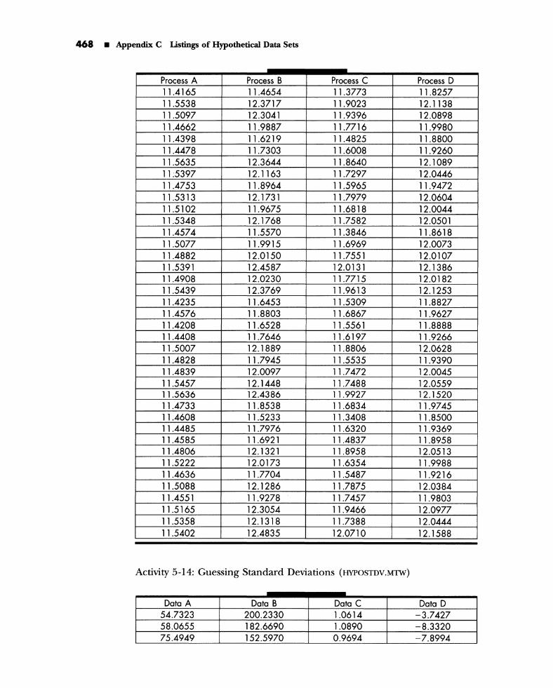
468 • Appendix C Listings of Hypothetical Data Sets
Process A Process B Process C Process D 11.4165 11.4654 11.3773 11.8257 11.5538 12.3717 11.9023 12.1138 11.5097 12.3041 11.9396 12.0898 11.4662 11.9887 11.7716 11.9980 11.4398 11.6219 11.4825 11.8800 11.4478 11.7303 11.6008 11.9260 11.5635 12.3644 11.8640 12.1089 11 ;5397 12.1163 11.7297 12.0446 11.4753 11.8964 11.5965 11.9472 11.5313 12.1731 11.7979 12.0604 11.5102 11.9675 11.6818 12.0044 11.5348 12.1768 11.7582 12.0501 11.4574 11.5570 11.3846 11.8618 11.5077 11.9915 11.6969 12.0073 11.4882 12.0150 11.7551 12.0107 11.5391 12.4587 12.0131 12.1386 11.4908 12.0230 11.7715 12.0182 11.5439 12.3769 11.9613 12.1253 11.4235 11.6453 11.5309 11.8827 11.4576 11.8803 11.6867 11.9627 11.4208 11.6528 11.5561 11.8888 11.4408 11.7646 11.6197 11.9266 11.5007 12.1889 11.8806 12.0628 11.4828 11.7945 11.5535 11.9390 11.4839 12.0097 11.7472 12.0045 11.5457 12.1448 11.7488 12.0559 11.5636 12.4386 11.9927 12.1520 11.4733 11.8538 11.6834 11.9745 11.4608 11.5233 11.3408 11.8500 11.4485 11.7976 11.6320 11.9369 11.4585 11.6921 11.4837 11.8958 11.4806 12.1321 11.8958 12.0513 11.5222 12.0173 11.6354 11.9988 11.4636 11.7704 11.5487 11.9216 11.5088 12.1286 11.7875 12.0384 11.4551 11.9278 11.7457 11.9803 11.5165 12.3054 11.9466 12.0977 11.5358 12.1318 11.7388 12.0444 11.5402 12.4835 12.0710 12.1588
Activity 5-14: Guessing Standard Deviations (HYPOSTDV.MTW)
Data A Data B Data C Data D 54.7323 200.2330 1.0614 -3.7427 58.0655 182.6690 1.0890 -8.3320 75.4949 152.5970 0.9694 -7.8994

• Appendix C Listings of Hypothetical Data Sets 469
Data A Data B Data C Data D 70.8519 176.1100 0.9964 -6.6365 67.5594 284.0310 0.9779 -8.5103 82.0604 210.7530 0.9920 -11.3988 67.3449 135.7440 1.0129 -2.9734 73.9735 167.4280 0.9910 -3.6779 59.9569 206.9280 0.9443 -0.1072 64.0481 127.0890 0.9710 -3.1872 70.4145 142.6490 1.0321 -3.3980 70.5806 225.1930 0.9837 -2.4381 70.5234 134.7350 0.9651 5.4287 59.6053 191.7320 1.0173 -1.4514 63.0206 177.6910 1.0044 -5.5888 57.1386 142.7390 0.9559 -3.4043 66.7414 172.8910 0.9539 -4.8423 66.2912 238.4620 1.0476 -4.4200 39.4021 343.0530 0.9888 -0.5386 70.4660 314.2950 1.0985 -9.1686 54.9322 182.8570 0.9819 -8.6683 70.0909 244.5870 0.9856 -14.3791 49.2586 236.8060 0.9920 -8.4293 62.5470 268.3330 0.9751 -14.4531 54.5510 244.9190 1.0732 -4.0124 78.2332 169.8710 1.0083 -2.9723 75.0430 226.4780 0.9905 -4.6135 74.6654 269.1320 0.8907 -5.1762 76.7585 203.2910 0.9641 -12.1286 83.1006 201.5240 1.0290 -12.3931 66.9678 167.4570 0.9312 0.1197 51.2948 102.8890 0.9725 -4.6073 79.2687 205.5250 1.1043 1.8484 68.5335 200.3780 1.0372 -1.4457 51.1347 220.1900 1.0607 -15.2446 53.6251 265.0840 1.0061 -1.9615 73.7969 221.6660 0.9644 -8.9919 61.4841 214.0470 0.9515 -6.0234 76.7655 263.5450 0.9307 -5.9924 54.0086 234.6190 1.0096 -0.1938 66.8219 205.1490 0.9744 -5.5941 55.5908 148.4350 0.9623 -8.6759 70.0916 260.8790 0.9661 -8.7433 63.3856 263.4330 0.9308 -2.1252 64.9589 182.7400 0.9820 -1.3464 74.9712 115.6500 1.0369 -11.2186 63.5829 270.8650 0.9952 -5.0162 65.8217 245.4750 1.0101 -0.9512 76.4025 126.9230 0.9952 -5.3799 53.4284 198.1700 0.9717 1.6207 64.9588 231.7590 0.9647 -2.7879

470 • Appendix C Listings of Hypothetical Data Sets
Data A Data B Data C Data D 46.9573 253.3560 0.9833 -4.8769 62.2297 241.4200 0.9930 -5.1715 71.0247 242.9490 1.0570 -6.1173 69.9688 261.1060 0.9557 0.5181 69.0292 172.6260 0.8707 -2.2005 53.4182 207.3680 1.0125 -1.2335 69.6185 179.3460 1.0678 -11.8271 57.9149 234.7990 1.0749 -3.4148 68.8708 174.7420 0.9809 -9.6962 68.5252 129.6640 0.9940 -9.9124 76.7544 95.4220 1.0030 -11.3669 64.6388 133.3370 0.9740 -4.3015 68.7167 263.5060 1.0385 -10.4150 54.8736 162.8340 0.9938 -9.1377 48.9441 251.2650 0.8861 -13.9931 58.3347 193.2390 1.0176 -16.0001 63.1308 223.1980 1.0385 -9.6562 38.8426 268.0770 1.0698 -8.9456 49.4594 130.5850 1.0769 3.9791 66.3701 228.6850 0.9678 -2.3438 69.3799 183.8290 1.0098 -9.5794 60.4799 142.1750 0.9816 -0.6389 73.7690 201.2340 0.9804 -2.6748 61.7042 266.1770 1.0372 2.1504 78.7420 240.5090 0.9559 -7.3905 41.3535 320.8660 1.0449 -5.1572 64.8503 177.7580 1.0209 -3.6856 60.8477 204.0690 0.9932 -13.5580 70.9215 119.6970 0.9964 -8.8984 58.0815 160.1130 1.0225 3.3616 63.3596 130.8600 0.9923 -8.0555 73.5292 204.0180 0.8370 2.6732 58.9281 226.8270 1.0737 -1.5957 65.5045 65.3540 0.9700 -0.4293 57.2830 265.8720 1.1029 -5.3904 54.3327 182.7050 1.0509 -0.8345 61.8720 197.8660 0.9651 -6.4203 76.2123 231.3630 1.0127 -15.0415 58.2271 146.0190 1.1274 -2.1868 88.1693 149.2930 1.0328 -4.1268 65.4506 206.2060 0.9670 -0.1929 60.7583 208.3380 0.9833 -6.0495 56.7109 272.6800 0.9848 -1.9930 80.8921 193.3570 1.0250 -10.1710 54.2190 238.9720 1.0252 -4.2453 66.8669 185.3370 1.0170 -0.7348 71.8376 168.8880 0.9294 -14.4362 59.6969 222.3630 1.0116 -6.9096 59.4178 172.1620 1.0410 -5.9749

• Appendix C Listings of Hypothetical Data Sets 471
Activities 7-2: Guess the Association; 8-1: Properties of Correlation (HYPOCORR.MTW)
Exam1 A Exam2 A Exam 1 B Exam2 B Exam1 C Exam2 C 72 78 78 78 69 72 79 74 75 63 84 55 69 67 88 77 55 83 76 77 73 78 78 62 56 60 85 68 67 76 60 60 78 73 81 61 64 65 76 67 57 84 78 70 68 70 57 80 78 71 76 60 72 67 68 74 67 75 83 56 74 77 76 67 61 79 66 79 60 57 77 62 74 82 58 52 73 68 83 85 66 66 68 74 82 77 66 78 64 77
Exam 1 D Exam2 D Exam1 E Exam2 E Exam1 F Exam2 F 79 62 99 96 55 68 67 61 59 56 57 61 62 70 75 76 64 68 64 78 58 58 64 70 82 59 82 83 64 59 81 69 77 77 73 64 71 68 95 95 64 77 63 67 58 61 67 56 67 65 65 65 85 56 63 75 68 69 68 57 57 75 68 66 60 64 59 74 59 58 69 66 65 74 89 85 73 59 80 58 56 59 59 70 68 67 84 80 67 60
Exam1 G Exam2 G Exam1 H Exam2 H Exam1 I Exam2 I Exam 1 J Exam2 J 49 95 49 54 12 17 37 39 52 81 52 57 52 62 44 41 55 69 55 60 55 52 32 33 58 59 58 62 58 73 37 34 61 51 61 65 61 69 35 41 64 45 64 68 64 71 41 45 67 41 67 70 67 72 42 33 70 39 70 73 70 80 45 36
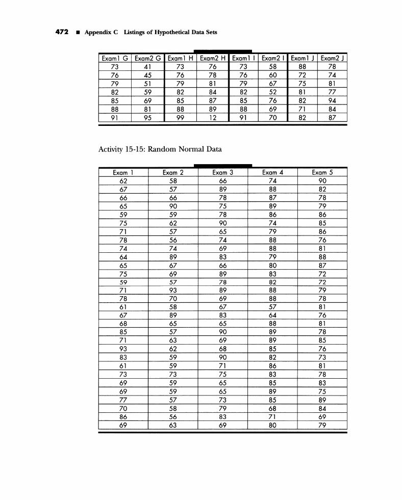
472 • Appendix C Listings of Hypothetical Data Sets
Exam1 G Exam2 G Exam1 H Exam2 H Exam1 I Exam2 I Exam1 J Exam2 J 73 41 73 76 73 58 88 78 76 45 76 78 76 60 72 74 79 51 79 81 79 67 75 81 82 59 82 84 82 52 81 77 85 69 85 87 85 76 82 94 88 81 88 89 88 69 71 84 91 95 99 12 91 70 82 87
Activity 15-15: Random Normal Data
Exam 1 Exam 2 Exam 3 Exam 4 Exam 5 62 58 66 74 90 67 57 89 88 82 66 66 78 87 78 65 90 75 89 79 59 59 78 86 86 75 62 90 74 85 71 57 65 79 86 78 56 74 88 76 74 74 69 88 81 64 89 83 79 88 65 67 66 80 87 75 69 89 83 72 59 57 78 82 72 71 93 89 88 79 78 70 69 88 78 61 58 67 57 81 67 89 83 64 76 68 65 65 88 81 85 57 90 89 78 71 63 69 89 85 93 62 68 85 76 83 59 90 82 73 61 59 71 86 81 73 73 75 83 78 69 59 65 85 83 69 59 65 89 75 77 57 73 85 89 70 58 79 68 84 86 56 83 71 69 69 63 69 80 79

• Appendix C Listings of Hypothetical Data Sets 473
Activities 24-2, 24-5, and 24-10: Hypothetical Sleeping Times (HYPOSLEE.MIW)
Sample 1 Sample 2 Sample 3 Sample 4 8.5 6.1 7.1 9.5 7.1 8.7 9.3 8.7 8.4 10.1 8.3 7.1 7.4 9.4 5.3 7.4 7.8 5.7 7.1 7.5 7.4 6.6 7.3 6.3 8.3 6.2 7.9 7.9 7.8 6.0 6.7 5.9 7.1 8.2 7.5 6.4 6.2 6.9 5.8 10.0 6.4 6.3 6.2 6.2 8.6 9.9 4.7 6.5 8.0 7.6 8.2 7.5 8.4 6.3 5.6 8.6 6.9 7.0 8.7 7.7 6.6 8.9 5.9 7.7 6.4 9.4 8.5 7.6 8.1 10.1 9.4 9.0 8.2 9.4 7.6 8.8 7.1 9.6 7.6 7.9
Activities 26-1 and 26-4: Hypothetical Commuting Times (HU'OCOMM.MlW)
Alex 1 Alex 2 Barb 1 Barb 2 Carl 1 Carl 2 19.3 23.7 16.4 24.4 23.7 27.7 20.5 24.5 17.6 27.1 24.3 28.5 23.0 27.7 20.2 32.0 25.5 29.1 25.8 30.0 21.0 34.0 26.8 30.2 28.0 31.9 23.8 35.1 28.0 32.1 28.8 32.5 26.4 36.1 28.4 32.4 30.6 32.6 30.4 37.8 29.3 34.0 32.1 35.5 30.6 38.3 30.1 34.6 33.5 38.7 31.6 41.3 30.6 35.3 38.4 42.9 32.0 43.9 33.3 36.1
Donna 1 Donna 2 10.1 24.9 28.4 32.4 20.4 27.7 32.4 36.4 13.5 25.0 28.5 33.3 22.4 28.6 32.5 36.6 20.9 25.8 28.9 33.4 24.2 28.9 33.8 37.2 21.7 26.0 29.0 33.8 24.4 28.9 33.9 37.3 23.7 26.1 29.3 33.8 24.4 29.4 34.0 37.5 22.8 26.5 29.8 34.0 25.0 29.5 34.9 38.0 23.0 26.6 30.1 35.3 25.4 30.4 35.4 39.7 23.5 26.7 30.0 36.6 25.6 30.4 35.5 41.5 24.0 27.1 30.2 39.5 26.2 31.0 35.5 44.4 24.8 28.0 33.2 39.9 27.2 31.2 36.1 46.2

Appendix D:
SOURCES FOR DATA SETS
Topic 1: Data and Variables I
• Activity 1-4: Data on physicians' gender are from The 1995 World Almanac and Book of Facts, p. 966.
• Activity 1-8: Data on sports' hazardousness are reported in the November 12, 1993, issue of the Harrisburg Evening-News.
Topic 2: Data and Variables II
• Activity 2-3: Data on tennis simulations are a random sample from the analysis in "Computer Simulation of a Handicap Scoring System for Tennis," by Allan Rossman and Matthew Parks, Stats: The Magazine for Students of Statistics, 10, 1993, pp. 14-18.
• Activity 2-6: Data on Broadway shows are from aJune 1993 issue of Variety magazine.
Topic 3: Displaying and Describing Distributions
• Activity 3-2: Data on British rulers are from The 1995 World Almanac and Book of Facts, pp. 534-535 .
• Activity 3-3: Data on college tuitions are from the October 23, 1991, issue of The Chronicle of Higher Education.
• Activity 3-7: Data on marriage ages were gathered by Matthew Parks at the Cumberland County (PA) Courthouse in June-July 1993.
475

476 • Appendix D Sources for Data Sets
• Activity 3-8: Data on Hitchcock films were gathered at a Blockbuster Video store in Carlisle, PA, inJanuary 1995.
• Activity 3-9: Data on dinosaur heights are from Jurassic Park by Michael Crichton, Ballantine Books, 1990, p. 165.
• Activity 3-10: Data on movies' incomes are from issues of Variety magazine in the summer of 1993.
• Activity 3-14: Data on Perot votes are from The 1993 World Almanac and Book of Facts, p. 73.
Topic 4: Measures of Center
• Activity 4-1: Data on Supreme Court service are from The 1997 World Almanac and Book of Facts, p. 189.
• Activity 4-3: Data on cancer pamphlets are from "Readability of Educational Materials for Cancer Patients," by Thomas H. Short, Helene Moriarty, and Mary Cooley, Journal of Statistics Education, 3, 1995.
• Activity 4-6: Data on planetary measurements are from The 1993 World Almanac and Book of Facts, p. 251.
• Activity 4-7: Data on the Supreme Court are from The 1995 World Almanac and Book of Facts, p. 85.
Topic 5: Measures of Spread
• Activity 5-6: Data on climate are from Tables 368-375 of the 1992 Statistical Abstract of the United States.
Topic 6: Comparing Distributions
• Activity 6-1: Data on shifting populations are from The 1995 World Almanac and Book of Facts, p. 379.
• Activity 6-2: Data on golfers' winnings are from the February 1991 issue of Golfmagazine.
• Activity 6-7: Data on automobile thefts are from Table 209 of the 1992 Statistical Abstract of the United States.
• Activity 6-8: Data on lifetimes are from The 1991 World Almanac and Book of Facts, pp. 336-374.
• Activity 6-11: Data on governors' salaries are from The 1995 World Almanac and Book of Facts, pp. 94-97.

• Appendix D Sources for Data Sets 477
• Activity 6-13: Data on cars are from Consumer Reports' 1995 New Car Yearbook. • Activity 6-15: Data on mutual funds are from the January 7, 1994, issue
of The Wall Street Journal. • Activity 6-16: data on Star Trek episodes are from Entertainment Weekly's
Special Star Trek Issue, 1994.
Topic 7: Graphical Displays of Association
• Activity 7-4: Data on O-ring failures are from "Lessons Learned from Challenger: A Statistical Perspective," by Siddhartha R. Dalal, Edward B. Folkes, and Bruce Hoadley, Stats: The Magazine Jor Students oj Statistics, 2, 1989, pp. 14-18.
• Activity 7-5: Data on fast food sandwiches are from a 1993 Arby's nutritional brochure.
• Activity 7-7: Data on airfares are from the January 8, 1995, issue of the Harrisburg Sunday Patriot-News and from the Delta Air Lines worldwide timetable guide effective December 15, 1994.
• Activity 7-11: Data on alumni donations are from the 1991-1992 Annual Report of Dickinson College.
• Activity 7-12: Data on peanut butter are from the September 1990 issue of Consumer Reports magazine.
• Activity 7-13: Data on SAT scores are from The 1997 World Almanac and Book oj Facts, p. 256.
Topic 8: Correlation Coefficient
• Activity 8-2: Data on televisions and life expectancy are from The 1993 World Almanac and Book oj Facts, pp. 727-817.
• Activity 8-14: Data on "Top Ten" rankings are from An Altogether New Book oj Top Ten Lists by David Letterman et al., Pocket Books, 1991, p. 44.
Topic 9: Least Squares Regression I
• Activity 9-7: Data on basketball salaries are from the June 24,1992, issue of USA Today.
478 • Appendix n Sources for nata Sets
Topic 10: Least Squares Regression II
• Activity 10-1: Data on gestation and longevity are from The 1993 World Almanac and Book of Facts, p. 676.
• Activity 10-6: Data on college enrollments are a sample from The 1991 World Almanac and Book of Facts, pp. 214-239.
Topic 11: Relationships with Categorical Variables
• Activity 11-2: Data on age and ideology are from Vital Statistics on American Politics by Harold W. Stanley and Richard G. Niemi, CQ Press, 1988, pp. 130-131.
• Activity 11-3: Data on AZT and HIV are reported in the March 7, 1994, issue of Newsweek.
• Activity 11-6: Data on toy advertising were supplied by Dr. Pamela Rosenberg.
• Activity 11-11: Data on living arrangements are from The 1995 World Almanac and Book of Facts, p. 961.
• Activity 11-12: Data on Civil War generals are summarized from Civil War General5 by James Spencer, Greenwood Press, 1986, pp. 121-138.
• Activity 11-13: Data on graduate admissions are from "Is There Sex Bias in Graduate Admissions?" by P. J. Bickel and J. W. O'Connell, Science, 187, pp. 398-404.
• Activity 11-14: Data on baldness and heart disease are from "A CaseControl Study of Baldness in Relation to Myocardial Infarction in Men," by Samuel M. Lasko et aI., Journal of the American Medical Association, 269, 1993, pp. 998-1003.
Topic 12: Random Sampling
• Activity 12-1: Data regarding the Elvis poll are reported in the August 18, 1989, issue of the Harrisburg Patriot-News. The data on the Literary Digest poll are from "Why the Literary Digest Poll Failed," by Peverill Squire, Public opinion Quarterly, 52, 1988, pp. 125-133.
• Activity 12-2: Data on U.S. Senators are from The 1997 World Almanac and Book of Facts, pp. 111-112.
• Activity 12-5: Data on polls regarding emotional support are reported in The Superpoll5ters by David W. Moore, Four Walls Eight Windows Publishers, p. 19.

• Appendix D Sources for Data Sets 479
• Activity 12-6: Data on alternative medicine are from a March 1994 issue of Self magazine.
• Activity 12-7: Data on courtroom cameras are reported in the October 4, 1994, issue of the Harrisburg Evening-News.
Topic 13: Sampling Distributions I: Confidence
• Activity 13-4: Data on Presidential voting are from The 1997 World Almanac and Book of Facts, p. 33.
• Activity 13-7: Data on American moral decline are from the June 13, 1994, issue of Newsweek.
• Activity 13-8: Data on cat households are from Table 392 of the 1992 Statistical Abstract of the United States.
Topic 15: Normal Distributions
• Activity 15-9: Data on family lifetimes were supplied by Anthony Kapolka.
Topic 16: Central Limit Theorem
• Activity 16-11: Data on non-English speakers are from The 1995 World Almanac and Book of Facts, p. 600.
Topic 17: Confidence Intervals I
• Activity 17-10: Data on television characters were reported in the June 28, 1994, issue of USA Today.
• Activity 17-12: Data on charitable contributions are from Table 603 of the 1992 Statistical Abstract of the United States.
480 • Appendix D Sources for Data Sets
Topic 18: Confidence Intervals II
• Activity 18-5: Data on dissatisfaction with Congress are from the October 27, 1994, issue of USA Today.
• Activity 18-12: Data on marital problems are from "Why Does Military Combat Experience Adversely Affect Marital Relations?" by Cynthia Gimbel and Alan Booth, Journal of Marriage and the Family, 56, 1994, pp. 691-703.
• Activity 18-13: Data on jury representativeness are from "Statistical Evidence of Discrimination," by David Kaye, Journal of the American Statistical Association, 77, 1982, pp. 773-783.
Topic 19: Tests of Significance I
• Activity 19-5: Data on teacher hiring are reported in Statistics for Lawyers, by Michael O. Finkelstein and Bruce Levin, Springer-Verlag, 1990, pp. 161-162.
Topic 21: Designing Experiments
• Activity 21-7: Data on UFO sightings are from "Close Encounters: An Examination of UFO Experiences," by Nicholas P. Spanos, Patricia A. Cross, Kirby Dickson, and Susan C. DuBreuil, Journal of Abnormal Psychology, 102, 1993, pp. 624-632.
• Activity 21-8: Data on Mozart music are reported in the October 14,1993, issue of Nature.
• Activity 21-11: Data on parolees are reported in the October 6, 1993, issue of The New York Times, p. B10.
Topic 22: Comparing Two Proportions I
• Activity 22-5: Data on wording of surveys are from Table 8.1 of Questions and Answers in Attitude Suroeys by Howard Schuman and Stanley Presser, Academic Press, 1981.
• Activity 22-6: Data on wording of surveys are from Tables 11.2, 11.3, and 11.4 of Questions and Answers in Attitude Suroeys by Howard Schuman and Stanley Presser, Academic Press, 1981.
• Activity 22-7: Data on smoking policies were supplied by Janet Meyer.

• Appendix D Sources for Data Sets 481
Topic 23: Comparing Two Proportions II
• Activity 23-2: Data on alcohol habits are from "Boozing and Brawling on Campus: A National Study of Violent Problems Associated with Drinking over the Past Decade," by Ruth C. Enge and David]. Hanson, journal of Criminal justice, 22, 1994, pp. 171-180.
• Activity 23-6: Data on the BAP Study are from "The Epidemiology of Bacillary Angiomatosis and Bacillary Peliosis," by Jordan W. Tappero et aI., journal of the American Medical Association, 269, 1993, pp. 770-775.
• Activity 23-8: Data on television sex are reported in Hollywood vs. America by Michael Medved, HarperCollins Publishers, 1992, pp. 111-112.
• Activity 23-9: Data on heart surgery are from a study by the Pennsylvania Health Care Cost Containment Council reported in the November 20, 1992, issue of the Harrisburg Patriot-News.
• Activity 23-10: Data on employment discrimination are reported in Statistics for Lawyers by Michael O. Finkelstein and Bruce Levin, SpringerVerlag, 1990, p. 123.
• Activity 23-12: Data on kids' smoking are reported in the October 4,1994, issue of the Harrisburg Patriot-News.
Topic 26: Comparing Two Means
• Activity 26-5: Data on baseball games were collected by Matthew Parks in June 1992.
• Activity 26-9: Data on classroom attention are from "Learning What's Taught: Sex Differences in Instruction," by Gaea Leinhardt, Andrea Mar Seewald, and Mary Engel, journal of Educational Psychology, 7I, 1979, pp. 432-439.

Index
ADDLINE • MTB, 150 Alternative hypothesis, 315
one-sided, 315, 328 two-sided, 315, 328
Analysis of variance, 441 Area under the curve, 247 Association
causation and, 135 concept of, 109 graphical displays of, 105-125
Assumptions, technical, 282 Averages, 52-55
Bar graphs, 8, 181 segmented, 182
BARGRAPH.MTB, 182 Biased sampling, 202, 302 Binary variables, 5 Blindness, 348 boxplot, 69, 90 Boxplots, 68-69
limitations of, 78-79 modified, 88
Case, 6 Case-control studies, 350 Categorical variables, 5, 113
relationships with, 177-196 Causation
association and, 135 Centers of distributions, 29
measures of, 47-63 Central Limit Theorem (CLT), 263-275 Chi-square tests, 441 Clinical trials, 350 CL T: see Central Limit Theorem Clusters of distributions, 30 Cohort studies, 350 Comparing
two means, 410 two proportions, 371-382
Comparisons, 346 paired, 410-442
Conditional distributions, 181 Confidence, 217-230 Confidence intervals, 279-309
for difference in population means, 422
for difference in population proportions, 373
for population mean, 391 for population proportion, 282 purpose of, 282
Confidence level, 282 Confounding variables, 135, 346 CONFSIM. MTB, 285 Control, 346 Control group, 346 Controlled experiments, 345 Convenience samples, 202 correlation, 129 Correlation coefficient, 127-144 Critical value, 282 Cross-sectional studies, 350 Curve
area under the, 247 normal, 245
Data, 3, 5 Data Window, 8 Degrees of freedom (d.f.), 391 Dependent variables, 108,346 describe, 52 Designing experiments, 343-355 df,: see Degrees of freedom Distributions, 7
centers of, 29 clusters of, 30 comparing, 81-101 conditional, 181 displaying and describing, 25-45 marginal, 181 normal, 243-262 peaks of, 30 sampling, 217-230 shapes of, 29-30
483
484 • Index
Distributions (continuer!) skewed to left, 30 skewed to right, 30 symmetric, 30 variability of, 29
dotplot,20 Dotplots, 19-20 Double-blind experiments, 348
Empirical rule, 72 Experiments
controlled, 346 designing, 343-355 double-blind, 348
Explanatory variables, 108, 346 Extrapolation, 151
Fail to reject Ho, 316 Fitted Line Plot, 150 Fitted value, 152 Five-number summary, 33, 68 Freedom, degrees of (d.f.), 391 Frequency, 8, 33
Granularity of distributions, 30 Graphical displays of association,
105-125 histogram, 34-35 Histogram, 33 hypothesized value, 315
Independence, 188 Independent sample, 419 Independent variables, 108, 346 Inference procedures
for comparing two population means, 410-442
for comparing two population proportions, 357-382
for single population mean, 385-417 for single population proportion,
279-339 Influential observation, 168 Intercept coefficient, 148 Interquartile range (IQR), 67
Labeled scatterplots, 113 Least squares line, 148 Least squares regression, 145-176 let, 10 Linear relationships, 131 logten,l71 Lower quartile, 67 Lurking variables, 135
Macros, ADDLINE . MTB, 150 BARGRAPH . MTB, 182 CONFSIM. MTB, 285 PINF.MTB, 286, 319 RANDCORR.MTB, 137 REESES . MTB, 221 SENATORS. MTB, 210 SIMSAMP. MTB, 225 2PSIM.MTB,361 2 PINF . MTB, 365 WIDGETS. MTB, 235
Margin-of-error, 298 Marginal distributions, 181 mean, 52 Mean, 49
sample, 390 trimmed,79
Means, comparing two, 410-442 Measurement variable, 5 Measures
of center, 47-63 resistant, 54 of spread, 65-80
median, 52 Median, 49 Midhinge,79 Midrange, 79 Mode, 49 Modified boxplots, 88
name,9 Negatively associated variables, 108 nonresponse, 202 Normal curve, 245 Normal distributions, 243-262
familyof,245 standard, 247
Null hypothesis, 315
Observation, influential, 168 Observational unit, 6 One-sided alternatives, 315-328 Outliers, 30, 166
p-value, 315, 327 Paired comparisons, 410, 442 Parameter(s), 208, 387 Peaks of distributions, 30 Percentile, 252 PINF.MTB, 286, 319 Placebo effect, 348 Population, 201, 208, 219 Population size, 301

Positively associated variables, 108 Practical significance, 333 Prediction, 149 print, 11 Probability, 247 Process, 219
simulating, 221, 359 Proportion of variability, 154
RANDCORR.MTB,137 Random digits, table of, 202 Random sampling, 199-215
simple (SRS), 202, 327 Randomization, 347 Range, 66 REESES . MTB, 221 regress, 149 Regression analysis, 440 Regression line, 148 Reject Ho, 316 Relationships, linear, 131 Relative frequency, 33 Residual, 152 residuals, 153 Residual plot, 170 Resistant measures, 54 Response, voluntary, 202 Response variables, 108,346
Sample, 201, 208, 219, biased, 202, 302 convenience, 202 independent, 419 margin-of-error, of, 298
Sample mean, 208 Sample proportions, 208
combined, 363 Sample size, 50, 211 Sampling, 201
biased,202 random, 199-216 simple random (SRS), 207
Sampling distributions, 217-230 Sampling variability, 209 Save Worksheet, 9 scatterplot, 114-115 Scatterplots, 107
labeled, 113 Segmented bar graphs, 182 SENATORS.MTB, 210 Session window, 8 set, 10 Shapes of distributions, 29 Side-by-side stemplot, 84
Significance, 231-242 practical, 333 statistical, 234, 237, 313, 333 tests of 237, 311-339 See also Significance test
Significance level, 316 Significance test
about population mean, 393, 405 about population proportion, 315 of equality of two population means,
423 of equality of two population
proportions, 362 Simple random sample (SRS), 202,
327 Simpson's paradox, 186 SIMSAMP.MTB, 225 Simulating process, 221, 359 Skewed distributions, 30 Slope, 147 Slope coefficient, 148 sort, 13 Spread, measures of, 65-80 SRS (simple random sample), 202, 327 stack,90 Standard deviation, 67 Standard normal distributions, 247 Standardization, technique of, 253 Standardized score, 73 Statistic(s), 208, 387
test, 315, 327 Statistical confidence, 282 Statistical significance, 234, 237, 313,
333 Statistical tendency, 86, 109 Stemplot, 31, 32
side-by-side, 84 subscripts, 90, 156 sum, 62 Symmetric distributions, 30
t* critical values, 392 t-distribution, 391 Table of random digits, 202 tally, 10 Tally, 8 Technical assumptions, 282 Tendency, statistical, 86, 109 Test decision, 316 Test statistic, 315, 327 Tests of significance, 237, 311-339
See also Significance test tinterval,395 Transforming variables, 170
• Index 485

486 • Index
Trials, clinical, 350 Trimmed mean, 79 ttest, 396 2psIM.MTB,361 2 PINF . MTB, 365 Two-sided alternative, 315, 328 Two-way tables, 180
unstack, 156 Upper quartile, 67
Variability, 7 of distributions, 29 proportion of, 154 sampling, 209
Variables, 5 binary, 5 categorical: see Categorical variables confounding, 135, 346
Variables (continued) dependent, 108,346 explanatory, 108,306 independent, 108, 346 lurking, 135 measurement, 5, 442 negatively associated, 108 positively associated, 108 response, 108, 346 transforming, 170
Variance, analysis of, 441 Voluntary response, 202
WIOOETS . MTB, 235
y-intercept, 147
z-score,73 z.* value, 283