İSTANBUL TECHNICAL UNIVERSITY ENERGY INSTITUTE …

İSTANBUL TECHNICAL UNIVERSITY �� ENERGY INSTITUTE

M.Sc. Thesis by Aziz Bora PEKİÇTEN

(301081003)

Date of submission : 06 May 2011 Date of defence examination: 06 June 2011

Supervisor (Chairman) : Prof. Dr. Bilge ÖZGENER (ITU) Members of the Examining Committee : Prof. Dr. Melih GEÇK İNLİ (ITU)

Prof. Dr. Cemal YILDIZ (ITU)

JUNE 2011

ASSEMBLY HOMOGENIZATION OF LIGHT WATER REACTORS BY A MONTE CARLO REACTOR PHYSICS METHOD AND VERIFICATION BY

A DETERMINISTIC METHOD

HAZ İRAN 2011

İSTANBUL TEKN İK ÜNİVERSİTESİ �� ENERJİ ENSTİTÜSÜ

YÜKSEK L İSANS TEZİ Aziz Bora PEKİÇTEN

(301081003)

Tezin Enstitüye Verildiği Tarih : 06 Mayıs 2011 Tezin Savunulduğu Tarih : 06 Haziran 2011

Tez Danışmanı : Prof. Dr. Bilge ÖZGENER (İTÜ) Diğer Jüri Üyeleri : Prof. Dr. Melih GEÇK İNLİ (İTÜ)

Prof. Dr. Cemal YILDIZ ( İTÜ)

HAFİF SU REAKTÖRLER İNİN MONTE CARLO REAKTÖR F İZİĞİ YÖNTEM İ İLE HOMOJEN İZASYONU VE DETERM İNİSTİK YÖNTEM

İLE DOĞRULANMASI

v

FOREWORD

I would like to express my deep appreciation and thanks for my advisors Dr. Tomasz Kozlowski and Prof. Dr. Bilge Özgener. And also I would like to thank to the Erasmus office in the European Union Centre of ITU, for giving me the chance to study abroad, and making possible this thesis work. This work is supported by Royal Institute of Technology Nuclear Power Safety Division and Istanbul Technical University Energy Institute.

May 2011

Aziz Bora Pekiçten

Mechanical Engineer

vii

TABLE OF CONTENTS

Page

ABBREVIATIONS ................................................................................................... ix LIST OF TABLES .................................................................................................... xi LIST OF FIGURES ................................................................................................ xiii SUMMARY .............................................................................................................. xv ÖZET ....................................................................................................................... xvii 1. INTRODUCTION .................................................................................................. 1

1.1 Purpose of The Thesis ........................................................................................ 2 2. ASSEMBLY HOMOGENIZATION METHODS ................ .............................. 3

2.1 Introduction ........................................................................................................ 3 2.2 Conventional Homogenization Theory .............................................................. 8

2.3 Koebke’s Equivalence Theory and Smith’s General Equivalence Theory ........ 9

3. DESCRIPTION OF TOOLS ............................................................................... 17

3.1 Introduction ...................................................................................................... 17 3.2 Serpent .............................................................................................................. 17 3.3 PARCS ............................................................................................................. 20

4. DESCRIPTION OF MINI CORE PROBLEMS ............................................... 23

4.1 Main Properties of The Core Assemblies ........................................................ 23

4.2 Application of The Verification and The Homogenization ............................. 24

4.2.1 Generation of the assembly discontinuity factors ..................................... 25

5. PRESENTATION AND DISCUSSION OF RESULTS ................................... 29 6. CONCLUSION ..................................................................................................... 33 REFERENCES ......................................................................................................... 35 APPENDICES .......................................................................................................... 37 CURRICULUM VITA ............................................................................................ 47

ix

ABBREVIATIONS

aADF : Average Assembly Discontinuity Factors ADF : Assembly Discontinuity Factors BWR : Boiling Water Reactors CANDU : Canada Deuterium Uranium Fig : Figure HTGR : High Temperature Gas Reactors Keff : K-effective (Effective Multiplication Factor) LWR : Light Water Reactors MCNP : Monte Carlo N-Particle PARCS : Purdue Advanced Reactor Core Simulator PWR : Pressurized Water Reactors U.S. NRC : United States Nuclear Regulatory Commission U-235 : Uranium isotope-235 UDF : Unity Discontinuity Factors UMN : University of Minnesota VTT : Technical Research Centre of Finland

xi

LIST OF TABLES

Page

Table 4.1: ADFs for fuel and reflector assemblies for combination-1...................... 26 Table 4.2: Comparison of solutions of combination-1 .............................................. 26



Table 5.1: Comparison of solutions of mini core-1 .................................................. 29









Table 5.10: Comparison of solutions of mini core-10 .............................................. 30





xiii

LIST OF FIGURES

Page

Figure 2.1 : A cell with fuel and moderator elements. ................................................ 3

Figure 2.2 : Wigner-Seitz approximation. .................................................................. 5

Figure 2.3 : Representation of the Newmarch effect. ................................................. 5

Figure 2.4 : Assembly homogenization. ..................................................................... 9

Figure 2.5 : Reactor core consisting of homogenized assemblies. ........................... 10

Figure 2.6 : Assembly (i,j). ....................................................................................... 11 Figure 4.1 : The cross section area of the fuel pin. ................................................... 23

Figure 4.2 : Geometry of combination-1. ................................................................. 25

Figure 4.3 : Geometry of combination-2. ................................................................. 25

Figure 4.4 : Geometry of combination-3. ................................................................. 26 Figure A.1 : Surface plots of errors of designing ADFs for combination-1 ............. 38 Figure A.2 : Surface plots of errors of designing ADFs for combination-2 ............. 39 Figure A.3 : Surface plots of errors of designing ADFs for combination-3 ............. 41 Figure B.1 : Configuration of the geometry for each core ........................................ 43

xv

ASSEMBLY HOMOGENIZATION OF LIGHT WATER REACTORS BY A MONTE CARLO REACTOR PHYSICS METHOD AND VERIFICATION BY A DETERMINISTIC METHOD

SUMMARY

Assembly homogenization is an important part of reactor core physics analysis. The loading of fuel assemblies in a commercial nuclear power plant is an important step before the startup of the reactor. The physical reactor core is modeled in computer environment. Distribution of fissile materials is decided after reactor physics code calculations. Many different reactor physics codes are used with calculations taking weeks or months. The purpose in this study is to test and verify the assembly homogenization capability of a Monte-Carlo reactor physics code called Serpent, which is used for the last years and is being used widely each year, and is faster than the previous ones.

In this study, Serpent did assembly homogenization of several different core configurations in two-dimensional geometry, and the results were tested in deterministic reactor simulation code called PARCS. Results showed that Serpent is capable to generate few-group constants for LWR-type assemblies. However, the assembly discontinuity factors generation by Serpent for fuel-reflector interface was not correct, so the objective of this thesis was to generate appropriate fuel-reflector discontinuity factors by off-line calculation, without access to the reference interface current. With the appropriately generated discontinuity factors, the results showed that assembly homogenization by Serpent is accurate to less than 0.5% keff error and less than 1.0% assembly flux ratio (the ratio of the averaged fast group of flux to the averaged thermal group of flux in the assembly).

xvii

HAFİF SU REAKTÖRLER İNİN MONTE CARLO REAKTÖR F İZİĞİ YÖNTEM İ İLE HOMOJEN İZASYONU VE DETERM İNİSTİK YÖNTEM İLE DOĞRULANMASI

ÖZET

Reaktör demet homojenizasyonu reaktör kalbi fiziksel analizlerinin önemli bir bölümüdür. Yakıt elemanlarının yüklenmesi, günümüz nükleer santrallerinde reaktörün çalışmasının başlangıcı öncesi için önemli bir adımdır. Fiziksel reaktör kalbi bilgisayar ortamında modellenir. Fisil maddelerin dağılımlarının kararı reaktör fiziği kodu hesaplamalarından sonra verilir. Hesaplamaları haftalar ve aylar süren bir çok farklı reaktör fiziği kodları vardır ve kullanılır. Bu çalışmanın amacı, son bir kaç yıldır kullanılan ve geçen her sene boyunca yaygınlaşan, öncekilere göre daha hızlı hesaplamalar yapabilen, Serpent adındaki Monte-Carlo reaktör fiziği kodunun homojenizasyon kabiliyetini test etmek ve doğrulamaktır.

Bu çalışmada değişik şekilde düzenlenmiş reaktör kalbi konfigürasyonlarının demet homojenizasyonu iki-boyutlu geometride Serpent kodu tarafından yapılmış ve sonuçlar deterministik reaktör simulasyon kodu olan PARCS ile kontrol edilmiştir. Sonuçlar Serpent kodunun hafif su reaktör tipi demetler için grup kesit alanı üretiminin uygun olduğunu gösterdi. Ama yakıt-reflektör arayüzü için demet devamsızlık faktörleri üretimi doğru değildi. Bu yüzden bu tezin amacı, referans arayüz akı verilerine sahip olmadan, kapalı bir yöntemle yakıt-reflektör arayüzü için doğru devamsızlık faktörleri üretimidir. Üretilen doğru devamsızlık faktörleri ile sonuçlar, Serpent kodu tarafından gerçekleştirilen demet homojenizasyonunun çok küçük hata yüzdesi ile yanlışsız olduğu görülmüştür. Hata yüzdeleri keff için 0.5%’in altında ve akı oranları (demet içindeki ortalama hızlı grup akısının ortalama termal grup akısına oranı) için 1.0%’in altında olduğu görülmüştür.

1

1. INTRODUCTION

Extensive knowledge of different quantities is necessary for the physics design and

analysis of light water reactors. The prediction of neutron density in space, direction

and energy increases the ability to perform core-follow calculations where the

determination of power distribution, control rod worth, shutdown margins and

isotopic depletion rates must be known. With the assumption that thermal-hydraulic

properties of the reactor and fundamental data are known, three-dimensional neutron

transport equation is a task need to be solved. Explicit modeling of water channels,

fuel pins, control rods and burnable poisons limits the direct methods of solving the

three-dimensional transport equation. Tools such as three-dimensional continuous

energy Monte Carlo and deterministic neutron transport methods are similarly

overwhelmed by the complexity of the computational problem of explicit

geometrical modeling on a core-wide basis.

Many reactor analysis methods circumvent the computational burden of explicit

geometrical modeling by coupling geometrically-simple, energy-intensive

calculations with few-group, geometrically-complicated calculations via spatial

homogenization and group condensation. The question how to make the best use of

spatial and spectral distributions of reaction rates and neutron densities has prompted

several different approaches to reactor analysis.

Alternative methods, which can all be put in a general class called nodal diffusion

methods have been developed over the years. These nodal methods have been

capable of solving three-dimensional neutron diffusion equation with a less than 2%

error in assemble-averaged powers using assembly-size mesh. The assumption of

these nodal methods is that to obtain “equivalent” diffusion theory parameters, which

are spatially constant over the whole cross sectional area of a fuel assembly, pin-by-

pin lattice cross sections have been spatially homogenized. The nodal solution

provides only nodal (volume-averaged) and surface (face-averaged) fluxes and

reaction rates. It is important that accurate methods for homogenizing reactor

assemblies are developed and employed.

2

1.1 Purpose of The Thesis

The major aim of this thesis is to perform assembly homogenization in two-

dimensional LWR mini-cores with possible fuel and reflector assembly

configurations. Homogenization techniques will be applied using Serpent (Monte

Carlo reactor physics code) and verified by PARCS (deterministic reactor simulation

code).

3

2. ASSEMBLY HOMOGENIZATION METHODS

2.1 Introduction

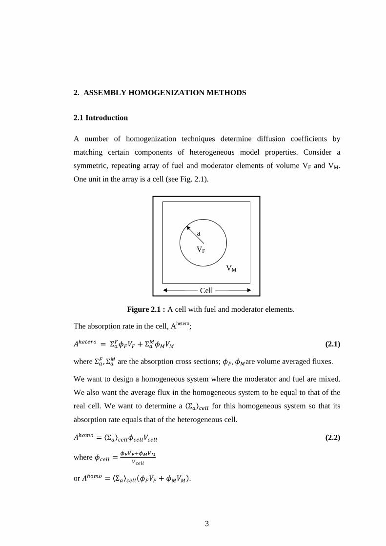
A number of homogenization techniques determine diffusion coefficients by

matching certain components of heterogeneous model properties. Consider a

symmetric, repeating array of fuel and moderator elements of volume VF and VM.

One unit in the array is a cell (see Fig. 2.1).

Figure 2.1 : A cell with fuel and moderator elements.

The absorption rate in the cell, Ahetero;

�� = Σ�� + Σ�� (2.1)

where Σ� , Σ� are the absorption cross sections; �� , ��are volume averaged fluxes.

We want to design a homogeneous system where the moderator and fuel are mixed.

We also want the average flux in the homogeneous system to be equal to that of the

real cell. We want to determine a ⟨Σ⟩�� for this homogeneous system so that its

absorption rate equals that of the heterogeneous cell.

�� = ⟨Σ⟩�� (2.2)

where �� = ��

or �� = ⟨Σ⟩�� + �� .

a

VF

VM

Cell

4

If A hetero equals to Ahomo, then;

⟨Σ⟩�� = !�� !��

(2.3)

Dividing the numerator and denominator by �� ;

⟨Σ⟩�� = !�� !�� ⁄ �#$�� ⁄ �# (2.4)

where % = ��

and is flux disadvantage factor. This methodology does not apply

directly to the diffusion coefficient “D” since it is related to leakage. For

multiregional cells (I>2);

⟨Σ&⟩�� = '(�∑ '* ��* �(⁄ �#*+*,-$�∑ ��* �(⁄ �#*+*,-

(2.5)

and %. = �*�(

, �� = ∑ �*�*+*,(��

.

A fuel assembly consists of a large number of pins, which might have differing

composition, each of which is clad and surrounded by moderator. A unit cell or pin

cell consist of a fuel pin, cladding and surrounding moderator. The first step in

homogenizing the fuel assembly is to homogenize each of the pin cells by calculating

the multigroup flux distribution in the fuel cell and using it to calculate homogenized

cross sections for the pin cell.

Although the calculation of the homogenized pin cell cross sections could be made

by combining an infinite medium calculation with some method for estimating the

disadvantage factor, today more advanced methods based on transport theory are

preferred.

A simplifying assumption is that the pin cell could be considered part of an infinite

array identical pin cells and thus reflective boundary conditions at cell boundary are

used to model such an infinite system. But existence of the fuel pin of differing

enrichment, control pins, burnable poisons etc. makes such an approach

questionable. The influence of the surroundings is usually introduced by specifying a

partial inward current J- and an albedo β.

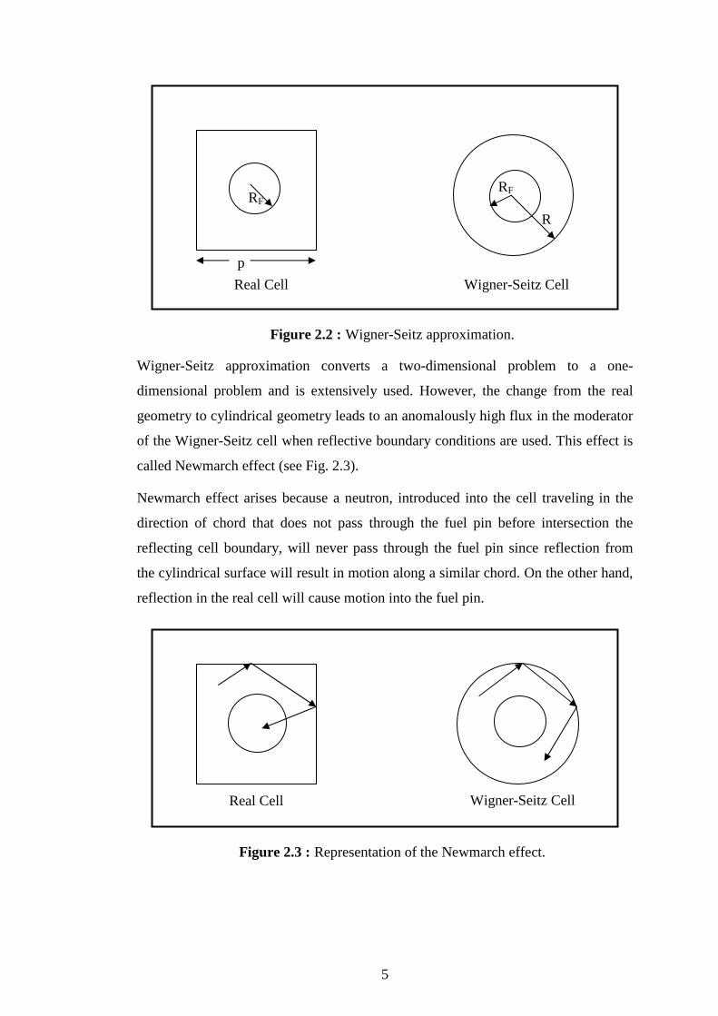
Since the fuel pin cells are cylindrical, it is convenient to approximate the actual pin

cell geometry by an equivalent cylindrical cell that preserves moderator volume. The

equivalent cylindrical cell is called Wigner-Seitz cell (see Fig. 2.2).

5

Figure 2.2 : Wigner-Seitz approximation.

Wigner-Seitz approximation converts a two-dimensional problem to a one-

dimensional problem and is extensively used. However, the change from the real

geometry to cylindrical geometry leads to an anomalously high flux in the moderator

of the Wigner-Seitz cell when reflective boundary conditions are used. This effect is

called Newmarch effect (see Fig. 2.3).

Newmarch effect arises because a neutron, introduced into the cell traveling in the

direction of chord that does not pass through the fuel pin before intersection the

reflecting cell boundary, will never pass through the fuel pin since reflection from

the cylindrical surface will result in motion along a similar chord. On the other hand,

reflection in the real cell will cause motion into the fuel pin.

Figure 2.3 : Representation of the Newmarch effect.

Real Cell Wigner-Seitz Cell

RF

p

Real Cell

RF

R

Wigner-Seitz Cell

6

Newmarch effect could be remedied by employing white boundary condition at the

cylindrical boundary. The white boundary condition assumes that a neutron that hits

the boundary will be returned with a cosine distribution, i.e. as if the returning

neutron comes from an infinite outside region with uniform isotopic sources. The

Wigner-Seitz approximation, combined with white reflection, gives excellent results

and is therefore well established in pin cell calculations.

If the pin cell-to-pin cell leakage is to be taken into account, the concept of albedo, or

reflection coefficient, is also employed. The albedo β,

/ = 012013

(2.6)

where “s” represents the cylindrical outer surface of the Wigner-Seitz cell.

Pin cell calculation are usually carried out using the collision probability method

based on integral transport equation since it involves scalar flux instead of angular

flux. But its basic drawback is the isotropic scattering assumption. To take linearly

anisotropic scattering at least approximately into account, there is a prescription,

called transport correction which is usually employed in collision probability

applications. Transport correction which involves the subtraction of the quantity

45Σ6,7. Transport corrected group cross sections are:

gsggstr

gs ,,0,, Σ−Σ=Σ µ (2.7)

gsggttr

gt ,,0,, Σ−Σ=Σ µ (2.8)

gsgggstr

ggs ,,0,, Σ−Σ=Σ →→ µ (2.9)

Usually the transport correction and the superscript “tr” is universally omitted. Once

pin cell homogenization is completed, the assembly is made up of a large number of

homogeneous regions (e.g. the homogenized, usually square, pin cells) surrounded

by structure, water gaps, control rods, etc.

The next step in the homogenization process is to perform a multigroup transport

calculation on the pin cell homogenized assembly for the purpose of obtaining

average group fluxes for each homogenized pin cell that can be used to calculate

homogenized cross sections that will allow the entire assembly to be represented as a

single homogenized region.

7

Any of the transport method or even diffusion theory in some cases can be used for

the full assembly transport calculation. Such calculations are normally performed

using reflective condition on the assembly boundary.

Heterogeneous system is described by multigroup transport theory as in (2.10).

( ) ( ) ( ) ( ) ( )∑∑=′

′′

=′′

→′ Σ+Σ=Σ+⋅∇G

gg

gf

gG

gg

ggg

gtg r

krrrrJ

11

vvvvvrr

φυχφφ (2.10)

We imagine that we know the solution to (2.10) and wish to use it to define

homogenized cross sections. We divide heterogeneous system into N

homogenization regions. We wish to define homogenized cross sections

Σ8�,.7 , Σ8.

7,→7, :Σ8;,.7 so that the homogenized transport equation:

( ) ( ) ( ) ( )∑∑=′

′′

=′′

→′ Σ+Σ=Σ+⋅∇G

gg

gif

gG

gg

ggig

gitg r

krrrJ

1,

1,

ˆ ˆˆ

ˆˆˆ ˆˆ vvvvrr

φυχφφ (2.11)

is obeyed for i=1,2…,N. Denoting the volume of the i’th homogenized region by Vi

and its k’th surface by <.=, we require:

( ) ( ) ( ) N ,1,2,i

,,,,x ˆˆ

, ∫∫ ==

Σ=Σii V

ggx

V

gg

ix

sftadVrrdVr

L

Krrr φφ (2.12)

and

( ) ( ) ( )iKkdSrJndSrJn

ki

ki S

g

S

g ,,2,1

N,1,2,i ˆ

L

Lrrrrrr

==

⋅=⋅ ∫∫ (2.13)

where K(i) is the number of surfaces of the i’th homogenization region. If (2.12) and

(2.13) are satisfied, obviously:

> = >8 (2.14)

Thus, homogenizes cross sections are defined by:

( ) ( )

( )∫

∫Σ=Σ

i

i

V

V

ggx

gix

dVr

dVrr

ˆ

ˆ

, r

rr

φ

φ (2.15)

and when diffusion theory is to be used in the homogenized calculation:

8

( )

( )∫

∫

∇⋅

⋅−

=

ki

ki

S

g

S

g

gik

dSrn

dSrJn

D ˆ

ˆrrr

rrr

φ (2.16)

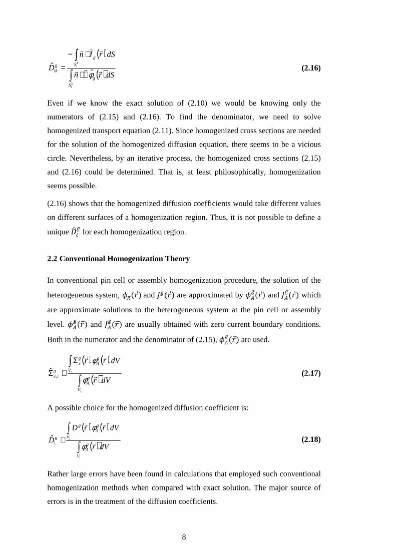
Even if we know the exact solution of (2.10) we would be knowing only the

numerators of (2.15) and (2.16). To find the denominator, we need to solve

homogenized transport equation (2.11). Since homogenized cross sections are needed

for the solution of the homogenized diffusion equation, there seems to be a vicious

circle. Nevertheless, by an iterative process, the homogenized cross sections (2.15)

and (2.16) could be determined. That is, at least philosophically, homogenization

seems possible.

(2.16) shows that the homogenized diffusion coefficients would take different values

on different surfaces of a homogenization region. Thus, it is not possible to define a

unique [email protected] for each homogenization region.

2.2 Conventional Homogenization Theory

In conventional pin cell or assembly homogenization procedure, the solution of the

heterogeneous system, �7�AB� and C7�AB� are approximated by �D7�AB� and CD

7�AB� which

are approximate solutions to the heterogeneous system at the pin cell or assembly

level. �D7�AB� and CD

7�AB� are usually obtained with zero current boundary conditions.

Both in the numerator and the denominator of (2.15), �D7�AB� are used.

( ) ( )

( )∫

∫Σ≅Σ

i

i

V

gA

V

gA

gx

gix

dVr

dVrr

ˆ

, r

rr

φ

φ (2.17)

A possible choice for the homogenized diffusion coefficient is:

( ) ( )

( )∫

∫≅

i

i

V

gA

V

gA

g

gi

dVr

dVrrD

D

ˆ

r

rr

φ

φ (2.18)

Rather large errors have been found in calculations that employed such conventional

homogenization methods when compared with exact solution. The major source of

errors is in the treatment of the diffusion coefficients.

9

The continuity of flux and current at interfaces between homogenization regions

seems also a source of problem. The homogenized diffusion equation, with

continuity of current and flux at interfaces, lacks sufficient degree of freedom to

preserve both reaction rates and surface currents. [1]

2.3 Koebke’s Equivalence Theory and Smith’s General Equivalence Theory

Equivalence theory involves assembly homogenization. Homogenization at the pin

cell level (see Fig. 2.4) is completed, and homogenized pin cell group cross sections

are assumed to be available:

Figure 2.4 : Assembly homogenization.

Since whole core calculations are usually carried out, after assembly

homogenization, by nodal methods, assembly homogenization involves variables

which are defined in the nodal method terminology. Equivalence homogenization is

closely associated with transverse integrated nodal methods. We assume a two

dimensional model of the assembly and assume the existence of an exact transport

solution for the assembly homogenized at the pin cell level. [2]

( ) ( ) ( ) ( ) ( ) ( ) ( )∑∑=′

′′

=′′

→′ Σ+Σ=Σ+⋅∇G

g

gf

gG

gg

ggg

gtg rr

krrrrrJ

1g

1

rrrrrrrrr

φυχφφ (2.19)

10

The equivalent homogenized assembly is a part of the reactor core and consists of

other homogenized assemblies. Each assembly is denoted by (i, j) where “i” denotes

the row number and “j” the column number (see Fig. 2.5).

Figure 2.5 : Reactor core consisting of homogenized assemblies.

We denote the cross sections of the homogenized assembly (i, j) by Σ8&,.,E and the flux

and the current by �8 and CBF respectively. The homogenized transport equation for

assembly (i, j) is:

( ) ( ) ( ) ( ) ( )ji,

1g,,

1,,, Vr , ˆ ˆˆ ˆ ˆˆ ∈Σ+Σ=Σ+⋅∇ ∑∑

=′′

′

=′

→′ rrrrrrr G

g

gjif

gG

gg

ggjig

gjitg r

krrrJ φυχφφ (2.20)

To inquire whether homogenization is theoretically possible, we assume that we

know the exact transport solution �7�AB� and CB7�AB� and try to determine the

homogenized constants Σ8&,.,E which would give reaction and leakage rates for the

homogenized assembly which are identical to their counterparts in the

nonhomogenized assembly.

(1,j)

(i,1) (1,1) (I,1)

(i,j) (I,j)

(I,j) (1,J) (I,J)

x1/2=0 x3/2 xi-1/2 xi+1/2 xI-1/2 xI+1/2 x

(i,j-1)

(i+1,j) (i-1,j)

(i+1,j+1)

y1/2=0

y3/2

yj-1/2

yj+1/2

yJ-1/2

yJ+1/2

y

11

We consider the assembly (i, j) (see Fig. 2.6):

Figure 2.6 : Assembly (i,j).

We integrate (2.19) over the assembly (i, j) to obtain:

( ) ( )∑∑

=′

′′

=′

′→′

−+−+

∆∆Σ+∆∆Σ

=∆∆Σ+−∆+−∆+−+−

G

gji

gji

gjif

G

gji

gji

ggji

jig

jig

jitg

jig

jiig

jig

jij

yxk

yx

yxJJxJJy

1,,,

g

1,,

,,,2/1,2/1,,2/1,2/1

φυχφ

φ (2.21)

where:

( )∫∫+

−

+

−∆∆

=2/1

2/1

2/1

2/1

, y

1

j,

j

j

i

i

y

y

g

x

xi

gji dydxyx

xφφ (2.22)

( ) ( )∫∫+

−

+

−

Σ∆∆

=Σ2/1

2/1

2/1

2/1

, , y

1

i,,,

j

j

i

i

y

y

ggx

x

xig

ji

gjix dydxyxyx

xφ

φ (2.23)

The edge averaged currents are defined as:

( )∫+

−

±± ⋅∆

=2/1

2/1

,x y

11/2i

j,2/1

j

j

y

y

gx

gji dyyJnJ m

rrm

(2.24)

( )∫+

−

±± ⋅∆

=2/1

2/1

,x x

11/2j

i2/1,

i

i

x

x

gy

gji dxyJnJ m

rrm

(2.25)

The (-) and (+) superscripts are used to denote location of the assembly (i, j) with

respect to the edge. If we integrate the homogenized equation similarly, we obtain:

( ) ( )∑∑

=′

′′

=′

′→′

−+−+

∆∆Σ+∆∆Σ

=∆∆Σ+−∆+−∆+−+−

G

gji

gji

gjif

G

gji

gji

ggji

jig

jig

jitg

jig

jiig

jig

jij

yxk

yx

yxJJxJJy

1,,,

g

1,,

,,,2/1,2/1,,2/1,2/1

ˆˆ ˆˆ

ˆˆˆˆˆˆ

φυχφ

φ (2.26)

(xi-1/2,yj-1/2) (xi+1/2,yj-1/2)

(xi+1/2,yj+1/2) (xi-1/2,yj+1/2)

(i,j)

∆xi

∆yi

12

where:

( )∫+

−

±± ⋅∆

=2/1

2/1

,xˆ y

1ˆ1/2i

j,2/1

j

j

y

y

gx

gji dyyJnJ m

rrm

(2.27)

( )∫+

−

±± ⋅∆

=2/1

2/1

,xˆ x

1ˆ1/2j

i2/1,

i

i

x

x

gy

gji dxyJnJ m

rrm

(2.28)

( )∫∫+

−

+

−∆∆

=2/1

2/1

2/1

2/1

,ˆ y

1ˆj

,

j

j

i

i

y

y

g

x

xi

gji dydxyx

xφφ (2.29)

Since we assume that we knew the heterogeneous exact solution, we choose the

homogenized constants such that:

gjix

gjix ,,,,

ˆ Σ=Σ (2.30)

If the quality of the edge currents in (2.21) and (2.26)can also be enforced, the cell

averaged fluxes of (2.21) and (2.26) would be equal:

gji

gji ,,

ˆ φφ = (2.31)

Thus both the reaction rates and the leakage through the edges would be identical to

the exact solution.

We have shown that an assembly homogenization, which preserves both reaction

rates and leakage, is possible if we knew the exact solution for the heterogeneous

assembly, which is possibly homogenized at the pin cell level. Moreover, the

homogenized diffusion coefficient seems to be arbitrary and has not been a factor in

our considerations.

The homogenized edge fluxes, are defined as:

( )

( )∫

∫

+

+

±±

±±

∆=

∆=

2/1

1/2-i

2/1

1/2-j

x

2/12/1,

y

2/1,2/1

dx , 1ˆ

dy , 1ˆ

i

j

x

jg

i

gji

y

ig

j

gji

yxx

yxy

m

m

m

m

φφ

φφ

(2.32)

would be discontinuous.

13

That is:

+−

+−

++

++

≠

≠g

jig

ji

gji

gji

2/1,2/1,

,2/1,2/1

ˆˆ

ˆˆ

φφ

φφ (2.33)

On the other hand, the exact fluxes:

( )

( )∫

∫

+

−

+

−

±±

±±

∆=

∆=

2/1

2/1

2/1

2/1

dx , 1

dy , 1

2/1,g

2/1,

2/1g

,2/1

i

i

j

j

x

x

jii

gji

y

y

ij

gji

yxx

yxy

m

m

m

m

φφ

φφ

(2.34)

are certainly continuous. That is:

+−

+−

++

++

=

=g

jig

ji

gji

gji

2/1,2/1,

,2/1,2/1

φφ

φφ (2.35)

At this point we define discontinuity factors:

( ) ( )

( ) ( )+

+

−

−

+

+

−

−

−

−

+

+

−

−

+

+

==

==

gji

gjiyg

jigji

gjiyg

ji

gji

gjixg

jigji

gjixg

ji

ff

ff

2/1,

2/1,,

2/1,

2/1,,

,2/1

,2/1,

,2/1

,2/1,

ˆ ,

ˆ

ˆ ,

ˆ

φφ

φφ

φφ

φφ

(2.36)

The imposition of (2.35) requires:

( ) ( )

( ) ( )

( ) ( )

( ) ( ) −−++

++−−

−−++

++−−

−−−

+++

−−−

+++

=

=

=

=

gji

xgji

gji

xgji

gji

xgji

gji

xgji

gji

xgji

gji

xgji

gji

xgji

gji

xgji

ff

ff

ff

ff

2/1,1,2/1,,

2/1,1,2/1,,

,2/1,1,2/1,

,2/1,1,2/1,

ˆ ˆ

ˆ ˆ

ˆ ˆ

ˆ ˆ

φφ

φφ

φφ

φφ

(2.37)

Thus, during whole core calculations, the homogeneous flux becomes discontinuous,

to preserve the continuity of the heterogeneous flux as in (2.35). However,

everything we have done so far has only theoretical value since the exact solution of

(2.19) will not be known. So we need an approximate solution to heterogeneous

problem (2.19). So we define the approximate solution �D7�AB� as the solution of:

( ) ( ) ( ) ( ) ( ) ( ) ( )∑∑=′

′′

=′

′→′ Σ+Σ=Σ+⋅∇G

g

gA

gf

gG

g

gA

gggA

gt

gA rr

krrrrrJ

11

rrrrrrrrr

φυχφφ (2.38)

14

with zero current boundary condition:

( ) Sr , 0 ∈=∇⋅rrrr

rn gAφ (2.39)

“S” is the union of the four sides of the assembly. Using approximate heterogeneous

solution �D7�AB� in (2.22), (2.23) and (2.29):

( ) ( )

( )∫∫

∫∫+

−

+

−

+

−

+

−

Σ

=Σ2/1

2/1

2/1

2/1

2/1

2/1

2/1

2/1

dy ,

dy , ,

ˆgA

gA

gx

,, j

j

i

i

j

j

i

i

y

y

x

x

y

y

x

xgjix

yx

yxyx

φ

φ

(2.40)

But (2.40) is no different than the result of the conventional homogenization theory.

So the homogenized cross sections have the same definition in the conventional and

equivalence homogenization theories. Diffusion coefficient is not needed for

establishing continuity of current across assemblies in equivalence theory. But since

it is still needed in whole core calculations, (2.40) could be employed to calculate

Σ8��,.,E7 . Then

gjitr

gjiD

,,, ˆ3

1

Σ= would give us the diffusion coefficient.

The only difference between the conventional and equivalence homogenization

theories is in the continuity of flux across assembly boundaries. Whereas

conventional theory assumes continuity, equivalence homogenization theory requires

discontinuity in homogenized solution as in (2.37). thus we need to evaluate the flux

discontinuity factors of (2.36) to apply equivalence homogenization theory. Since the

numerators in (2.36) involve g ji ,2/1+φ etc., which we do not know, we approximate

with gjiA ,2/1, +φ . The denominators in (2.36) have to be the homogeneous counterpart

of the heterogeneous approximate solution �D7�AB�. We call it �8D

7�AB�.

Since �D7�AB� involves zero-current boundary condition at assembly boundary, �8D

7�AB�

is subject to the same boundary conditions. Since �8D7�AB� is the solution of a

homogenized system (spatially constant cross section), and zero-current boundary

condition makes it a part of an infinite system, �8D7�AB� is constant. That is:

gjiA

gjiA

gjiA

gjiA

gjiA ,,2/1,,2/1,,,2/1,,2/1,

ˆˆˆˆˆ φφφφφ ====+−+−

−+−+ (2.41)

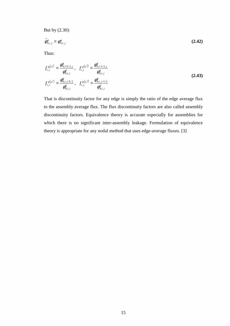
15

But by (2.30):

gjiA

gjiA ,,,,

ˆ φφ = (2.42)

Thus:

( ) ( )

( ) ( )g

jiA

gjiAyg

jigjiA

gjiAyg

ji

gjiA

gjiAxg

jigjiA

gjiAxg

ji

ff

ff

,,

2/1,,,

,,

2/1,,,

,,

,2/1,,

,,

,2/1,,

,

,

φφ

φφ

φφ

φφ

−+

−+

==

==

+−

+−

(2.43)

That is discontinuity factor for any edge is simply the ratio of the edge average flux

to the assembly average flux. The flux discontinuity factors are also called assembly

discontinuity factors. Equivalence theory is accurate especially for assemblies for

which there is no significant inter-assembly leakage. Formulation of equivalence

theory is appropriate for any nodal method that uses edge-average fluxes. [3]

17

3. DESCRIPTION OF TOOLS

3.1 Introduction

The purpose of this study is to verify the results for a defined core configuration

created by a Monte Carlo reactor physics code with a deterministic reactor physics

code. The Monte Carlo reactor physics code used in this thesis work is called

Serpent, which is a code developed by VTT. The deterministic code is three-

dimensional reactor simulator code called PARCS developed by Purdue University

and U.S. NRC.

3.2 Serpent

Serpent is a three-dimensional Monte Carlo reactor physics code developed at VTT

since 2004. The code is specialized in two-dimensional lattice physics calculations

but it is possible to model complicated three-dimensional geometries also. The code

is capable of generating homogenized multi-group constants for deterministic reactor

core simulators, burn-up calculations for fuel cycle studies and research reactors,

demonstration of reactor physics phenomena and for educational studies.

Serpent uses a universe-based geometry where it is easy to describe two or three-

dimensional designs. Material cells and surface types are the basis of the geometry.

There are many features to describe cylindrical fuel pins and spherical fuel particles,

square and hexagonal lattices, circular cluster arrays for CANDU fuels, and fuel

definition for HTGR cores.

Combination of conventional surface-to-surface ray-tracing and the Woodcock delta-

tracking method have an efficient geometry routine for lattice calculations. The

track-length estimate of neutron flux in delta-tracking is not efficient for small or thin

volumes located far from active source.

18

Serpent reads cross sections from ACE format libraries where classical collision

kinematics and ENDF reaction laws are the basis of the interaction physics. The data

in libraries is available for 432 nuclides at temperatures of 300, 600, 900, 1200, 1500

and 1800 K.

Burn-up calculations can be executed as a part or complete application. However,

memory usage might be a limiting factor for large systems when defining the number

of depletion zones. There is no need for an additional user effort for selection of

fission products and actinide daughter nuclides and the irradiation history is defined

in units of time and burn-up. Reaction rates are normalized to total power, specific

power density, flux or fission rate.

It can produce homogenized multi-group constants for deterministic reactor core

simulators, which is important for the current work. The standard output contains:

• Effective and infinite multiplication factors calculated using different

methods

• Homogenized few-group cross sections

• Group-transfer probabilities and scattering matrices

• Diffusion coefficients calculated using two fundamentally different methods

• Pn scattering cross sections up to order 5

• Assembly pin-power distributions

Homogenization can be done for multiple universes where group constants for

several assemblies are produced within a single run. The user defines the number and

borders of few-energy groups for the group constant generation.

The results for burn-up calculation are given as material-wise and total values, and

consist of isotopic compositions, transmutation cross sections, activities and decay

heat data.

All numerical output is written in MATLAB m-format files for simplification of

post-processing of several calculation cases. A geometry plotter feature and a

reaction rate plotter are also available for the code.

19

Serpent has been widely validated in light water reactor lattice calculations. Results

for effective multiplication factors and homogenized few-group cross sections are

within the statistical accuracy from reference MCNP results when the same ACE

libraries are used.

Comparison to a similar calculation suggests that Serpent may run 80 times faster

than codes like MCNP. The reason of the difference is not from the efficiency of the

code but rather from the fact of large reaction rate tallies of MCNP. The important

point is that Serpent can run full-scale assembly burn-up calculations similar to

deterministic transport codes, and overall calculation time is counted in hours or

days, rather than weeks or months. [4]

Monte Carlo (MC) methods are stochastic techniques, meaning they are based on the

use of random numbers and probability statistics to investigate problems. You can

find MC methods used in everything from economics to nuclear physics to regulating

the flow of traffic. Of course the way they are applied varies widely from field to

field, and there are dozens of subsets of MC even within chemistry. But, strictly

speaking, to call something a "Monte Carlo" experiment, all you need to do is use

random numbers to examine some problem.

The use of MC methods to model physical problems allows us to examine more

complex systems than we otherwise can. Solving equations which describe the

interactions between two atoms is fairly simple; solving the same equations for

hundreds or thousands of atoms is impossible. With MC methods, a large system can

be sampled in a number of random configurations, and that data can be used to

describe the system as a whole.

The Monte Carlo method provides approximate solutions to a variety of

mathematical problems by performing statistical sampling experiments on a

computer. The method applies to problems with no probabilistic content as well as to

those with inherent probabilistic structure. Among all numerical methods that rely on

N-point evaluations in M-dimensional space to produce an approximate solution, the

Monte Carlo method has absolute error of estimate that decreases as N superscript -

1/2 whereas, in the absence of exploitable special structure all others have errors that

decrease as N superscript -1/M at best.

20

3.3 PARCS

PARCS is a three-dimensional reactor core simulator which solves the steady-state

and time-dependent, multi-group neutron diffusion and SP3 transport equations in

orthogonal and non-orthogonal geometries. PARCS is coupled directly to the

thermal-hydraulics system code TRACE from which flow field information and

temperature are provided to PARCS during transient calculations.

The major calculation features in PARCS are eigenvalue calculations, transient

(kinetics) calculations, and adjoint calculations for commercial LWRs. Three-

dimensional calculation model is the primary use of PARCS for the realistic

representation of the physical reactors. However, for faster simulations for a group of

transients, one-dimensional modeling is available when dominant variation of the

flux is in the axial direction.

The input system in PARCS is card name based while default input parameters are

maximized and the amount of the input data is minimized. For the continuation of the

transient calculations, a restart feature is available, where the calculation restarts

from the point that restart file was written. Various edit options are available in

PARCS, also an on-line graphics feature that provides a quick and versatile

visualization of the various physical phenomena occurring during transient

calculation.

Accomplishing different tasks with high efficiency is established by incorporating

numerous sophisticated spatial kinetics methods into PARCS. For spatial

discretization, a variety of solution kernels are available to include the most popular

LWR two group nodal methods, the Analytic Nodal Method (ANM) and the Nodal

Expansion Method (NEM).

The usage of the advanced numerical solution methods minimizes the computational

burden. The eigenvalue calculation to establish the initial steady-state is performed

using the Wielandt eigenvalue shift method. When using the two nodal group

methods, a pin power reconstruction method is available in which predefined

heterogeneous power form functions are combined with a homogeneous intranodal

flux distribution.

21

Two modes are available for one-dimensional calculations: normal one-dimensional

and quasi-static one-dimensional. The normal one-dimensional mode uses a one-

dimensional geometry and precollapsed one-dimensional group constants, while the

quasi-static one-dimensional keeps the three-dimensional geometry and cross

sections but performs the neutronic calculation in the one-dimensional mode using

group constants which are collapsed during the transient. To preserve the three-

dimensional planar averaged currents in the subsequent one-dimensional

calculations, current conservation factors are employed in one-dimensional

calculations during one-dimensional group constant generation. PARCS is also

capable of performing core depletion analysis by introducing burn-up dependent

macroscopic cross sections.

The calculation features of PARCS are as follows;

• Eigenvalue calculation

• Transient calculation

• Xenon/Samarium calculation

• Decay heat calculation

• Pin power calculation

• Adjoint calculation

There are many PARCS calculation methods, which are directly related to execution

control, which users can choose the proper options suiting best for their needs. The

method used for this thesis is 2 group nodal methods. The spatial solution of the

neutron flux in the reactor is determined in PARCS using well-established numerical

methods. Nodal methods are the primary means used in PARCS to obtain higher

order solutions to the neutron diffusion equation solving the two-node problem.

The ANM is regarded as one of the more accurate techniques for solving the neutron

diffusion equation. The only approximation required is that used for the shape of the

transverse leakage sources which appear in the one-dimensional, transverse

integrated flux equations. Although the analytic nature of this method is responsible

for its remarkable accuracy, it has thus far lead to algebraically complicated

expressions for the nodal coupling relations which, for all practical purposes, appears

to restrict the ANM to only two energy group problems. This apparent limitation is

22

not due to the method itself, but arises as a result of the original approach taken for

the evaluation of the nodal coupling relations. The preparation of these coupling

coefficients relies on the evaluation of trigonometric functions of G by G matrices.

These expressions become increasingly complicated as the number of energy groups

increases.

The first polynomial method was NEM. In fact, although some variations and

improvements have been considered, the NEM ideology still dominates the

polynomial class of nodal methods. In this lowest order form, NEM considers a

quadratic expansion of the transverse averaged flux (i.e. φj(x) and φi(y)) on each cell.

The expansion coefficients are determined by applying Fick’s law in combination

with discrete nodal balance equation and continuity of normal current. Considerable

effort has been made to utilize higher order polynomial expansion within NEM. The

difficulty this creates is centered around the evaluation of the higher order expansion

coefficients. In particular, the weighted residual procedure that is typically used

relies on transverse-integrated and as a result an approximation of the transverse

normal currents (i.e. transverse leakage) is also required.

ANM in PARCS has been used frequently within the LWR industry to solve the two-

group diffusion equation. When there is no net leakage out of a node and the ANM

matrix becomes singular, the problem is called as critical node problem and methods

were added to PARCS to address this problem. The second nodal method, NEM was

added which does not have this potential problem, but is less accurate for certain

types of problems. Replacement of ANM two-node problem by a NEM two-node

problem for the near critical nodes is available with a hybrid ANM-NEM method.

The user specifies a tolerance on the difference in the node kinf and keff which is used

to switch between the ANM and NEM kernels. NEM is also available in a multi-

group form for both Cartesian and hexagonal geometries. [5]

4. DESCRIPTION OF MINI CORE PROB

The major work done on this thesis

fuel-reflector interface without explicit knowledge of heterogeneous interface

conditions and verifying the

purpose is to achieve

average thermal flux

4.1 Main Properties

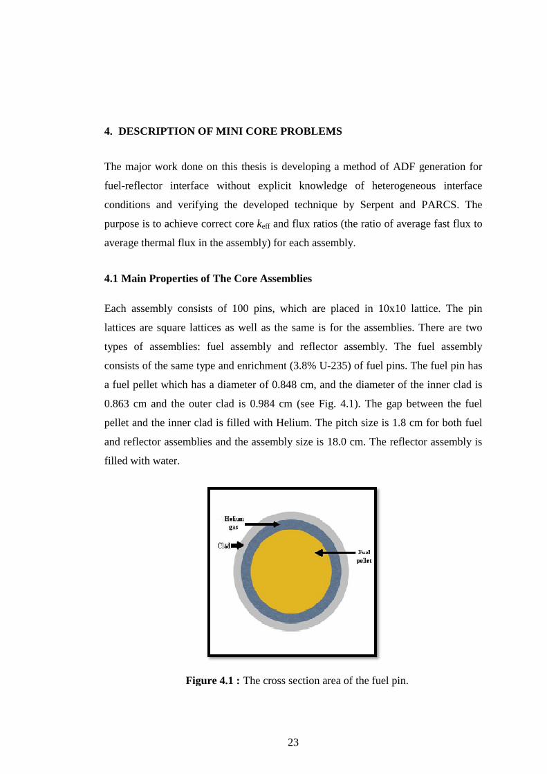
Each assembly consists of 100 pins, which are placed

lattices are square lattices as well as the same is for the assemblies. There are two

types of assemblies: fuel assembly and reflector assembly.

consists of the same type and enrichment

a fuel pellet which has a diameter of 0.848 cm

0.863 cm and the outer clad is 0.984 cm

pellet and the inner clad is filled with Helium.

and reflector assemblies and the assembly size is 18.0 cm.

filled with water.

Figure 4.1 :

23

DESCRIPTION OF MINI CORE PROB LEMS

e major work done on this thesis is developing a method of ADF generation for

reflector interface without explicit knowledge of heterogeneous interface

verifying the developed technique by Serpent

achieve correct core keff and flux ratios (the ratio of

in the assembly) for each assembly.

Main Properties of The Core Assemblies

Each assembly consists of 100 pins, which are placed in 10x10

tices are square lattices as well as the same is for the assemblies. There are two

types of assemblies: fuel assembly and reflector assembly. The fuel assembly

type and enrichment (3.8% U-235) of fuel pins. The fuel pin has

et which has a diameter of 0.848 cm, and the diameter of

the outer clad is 0.984 cm (see Fig. 4.1). The gap between the fuel

pellet and the inner clad is filled with Helium. The pitch size is 1.8 cm for both fuel

reflector assemblies and the assembly size is 18.0 cm. The reflector assembly is

Figure 4.1 : The cross section area of the fuel pin

is developing a method of ADF generation for

reflector interface without explicit knowledge of heterogeneous interface

and PARCS. The

average fast flux to

10x10 lattice. The pin

tices are square lattices as well as the same is for the assemblies. There are two

The fuel assembly

fuel pins. The fuel pin has

, and the diameter of the inner clad is

The gap between the fuel

The pitch size is 1.8 cm for both fuel

The reflector assembly is

The cross section area of the fuel pin.

24

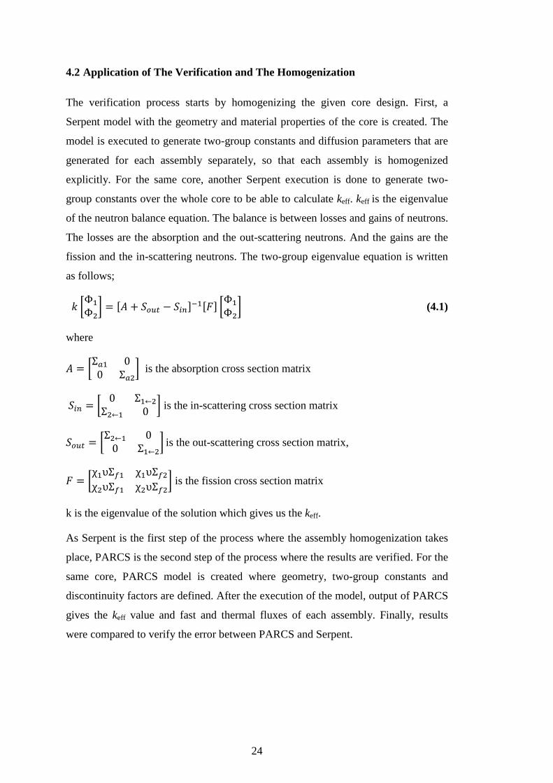
4.2 Application of The Verification and The Homogenization

The verification process starts by homogenizing the given core design. First, a

Serpent model with the geometry and material properties of the core is created. The

model is executed to generate two-group constants and diffusion parameters that are

generated for each assembly separately, so that each assembly is homogenized

explicitly. For the same core, another Serpent execution is done to generate two-

group constants over the whole core to be able to calculate keff. keff is the eigenvalue

of the neutron balance equation. The balance is between losses and gains of neutrons.

The losses are the absorption and the out-scattering neutrons. And the gains are the

fission and the in-scattering neutrons. The two-group eigenvalue equation is written

as follows;

> GΦ$ΦIJ = K� + <�L� − <.NOP$KQO GΦ$ΦI

J (4.1)

where

� = GΣ$ 00 ΣI

J is the absorption cross section matrix

<.N = G 0 Σ$←IΣI←$ 0 J is the in-scattering cross section matrix

<�L� = GΣI←$ 00 Σ$←I

J is the out-scattering cross section matrix,

Q = Gχ$υΣ;$ χ$υΣ;IχIυΣ;$ χIυΣ;I

J is the fission cross section matrix

k is the eigenvalue of the solution which gives us the keff.

As Serpent is the first step of the process where the assembly homogenization takes

place, PARCS is the second step of the process where the results are verified. For the

same core, PARCS model is created where geometry, two-group constants and

discontinuity factors are defined. After the execution of the model, output of PARCS

gives the keff value and fast and thermal fluxes of each assembly. Finally, results

were compared to verify the error between PARCS and Serpent.

25

4.2.1 Generation of the assembly discontinuity factors

The basic parameters, which are converted from one code to the other, are few-group

constants and assembly discontinuity factors. Serpent is capable to generate the

correct few-group constants for single and multi-assembly problem but it is not

capable of generating correct ADFs for multi-assembly problem. The ADFs were

generated off-line for a set of 2x2 cores (see Fig. 4.4, Fig. 4.5 and Fig. 4.6) in a

typical fuel-reflector configuration.

Figure 4.2 : Geometry of combination-1.


26


The two-group constants for each assembly were generated by Serpent and then

introduced into the cross section card of PARCS. To be able to find the ADFs that

give the best keff and best flux ratio results, a set of ADFs was generated and tested

with a value region of 0.01 to 1.0.

The keff and flux ratio results were compared with the reference and the optimum

ADF was found. The final choice of ADFs and the results for each combination are

seen at the Table from 4.1 to 4.6 (detailed plots of the results are given in the

Appendix A.1, A.2 and A.3).

Table 4.1: ADFs for fuel and reflector assemblies for combination-1

Composition ADF fast group ADF thermal group F1, F2 1.0 1.0 R1, R2 0.54 0.55

Table 4.2: Comparison of solutions of combination-1

keff

Assembly F1 Flux Ratio


Assembly R1 Flux Ratio


Reference solution

1.26721 2.325 2.325 0.375 0.376

UDF solution +1.8% -0.4% -0.4% +4.9% +4.9% ADF solution 0.0% -0.1% -0.1% -0.6% -0.6%


Composition ADF fast group ADF thermal group F1, F2, F3 1.0 1.0

R 0.62 0.57

27


keff




Assembly R Flux Ratio

Reference solution

1.34083 2.356 2.283 0.282 0.401

UDF solution +0.9% +0.3% +0.1% +0.1% +5.0% ADF solution 0.0% +0.4% +0.3% +0.3% -1.9%


Composition ADF fast group ADF thermal group F 1.0 1.0

R1, R2, R3 0.40 0.56


keff

Assembly F Flux Ratio




Reference solution

1.12928 2.336 0.381 0.381 0.293

UDF solution +4.1% -0.7% +5.1% +5.0% -4.5% ADF solution 0.0% -0.7% +1.0% +0.9% -5.7%

Reference solution is the result from Serpent, UDF solution is the results without

ADFs and ADF solution is the results with ADFs. The results prove that the ADFs

make a remarkable improvement in keff and flux ratios prediction.

In addition, it is seen that the thermal ADF in each three case is very close to each

other. As the thermal group ADF is more important than the fast group ADF, in the

mini core problems it is also possible to use average ADFs (aADFs) which will be

the average of the three cases that ADFs were generated.

29

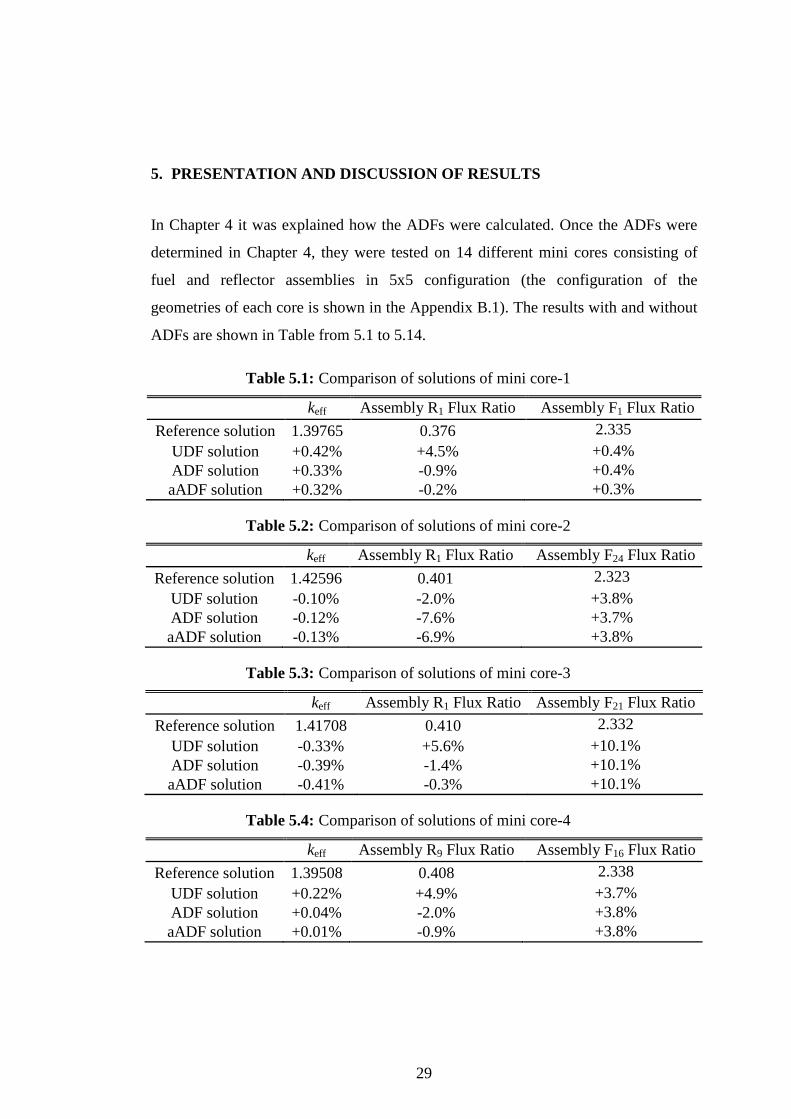
5. PRESENTATION AND DISCUSSION OF RESULTS

In Chapter 4 it was explained how the ADFs were calculated. Once the ADFs were

determined in Chapter 4, they were tested on 14 different mini cores consisting of

fuel and reflector assemblies in 5x5 configuration (the configuration of the

geometries of each core is shown in the Appendix B.1). The results with and without

ADFs are shown in Table from 5.1 to 5.14.

Table 5.1: Comparison of solutions of mini core-1

keff Assembly R1 Flux Ratio Assembly F1 Flux Ratio

Reference solution 1.39765 0.376 2.335 UDF solution +0.42% +4.5% +0.4% ADF solution +0.33% -0.9% +0.4% aADF solution +0.32% -0.2% +0.3%



Reference solution 1.42596 0.401 2.323 UDF solution -0.10% -2.0% +3.8% ADF solution -0.12% -7.6% +3.7% aADF solution -0.13% -6.9% +3.8%



Reference solution 1.41708 0.410 2.332 UDF solution -0.33% +5.6% +10.1% ADF solution -0.39% -1.4% +10.1% aADF solution -0.41% -0.3% +10.1%




30



Reference solution 1.26674 0.379 2.326 UDF solution +1.91% +4.4% -0.5% ADF solution +0.03% -1.2% -0.2% aADF solution +0.11% -0.6% -0.4%












Reference solution 1.25739 0.378 2.396 UDF solution +1.75% +6.0% +4.0% ADF solution +0.29% +0.6% +4.2% aADF solution +0.34% +1.4% +4.1%



Reference solution 1.29401 0.408 2.379 UDF solution +1.06% +6.3% +5.8% ADF solution -0.16% +0.2% +5.9% aADF solution -0.07% 0.0% +5.9%

31



Reference solution 1.38662 0.400 2.337 UDF solution +0.28% +5.9% +3.4% ADF solution -0.05% -1.1% +3.5% aADF solution -0.14% -0.1% +3.5%



Reference solution 1.41511 0.432 2.329 UDF solution +0.14% +5.0% +0.5% ADF solution -0.01% -3.1% +0.5% aADF solution -0.05% -2.0% +0.5%






Reference solution 1.32844 0.371 2.362 UDF solution +1.09% +5.1% +0.3% ADF solution +0.19% -0.8% +0.4% aADF solution -0.04% -0.5% +0.4%

In general, the error in the results reduces remarkably with the use of ADFs. We can

see that the generated few-group constants by Serpent are reliable, because the

reduction error occurs with the use of correctly designed ADFs.

The three different discontinuity factor solutions (UDF, ADF and aADF) gave the

same flux ratio results for the fuel assemblies because the value of the discontinuity

factors in each solution is always 1.0 for fuel assemblies. However, the ADF and

aADF solutions for the reflector assemblies, which have at least one interface with

the fuel assemblies, had a remarkable improvement in the flux ratio results.

32

The ADF and aADF solutions always gave very good keff results. However, the UDF

solution gave inconsistent keff results. The inconsistency is because of the number of

the fuel assemblies in each configuration. The configurations which had a high

number of fuel assemblies gave closer keff results to the reference solution, because

there were fewer reflector assemblies, where the flux distribution was not correct.

However, when the number of reflector assemblies increased, the UDF solution gave

bad keff results.

The thermal flux group is more important than the fast flux group in light water

reactors. The value of aADF thermal discontinuity factor is very similar to the values

of ADF thermal discontinuity factor. Therefore, aADF solution gave similar results

as ADF solution.

33

6. CONCLUSION

The major purpose of this research was to verify the assembly homogenization

capability of Serpent. Since assembly power distribution is very important for

commercial reactors, the study is important for the application of Serpent as a tool

for cross section homogenization. The conclusion for few-group constant generation

is that Serpent is capable to generate few-group constants that can be used in a

deterministic reactor code. However, generation of ADFs for fuel-reflector interface

has to be done off-line by a separate method, as presented in this thesis. The effect of

ADFs is significant and cannot be neglected. With correct ADFs, the homogeneous

nodal solution errors were acceptable for every mini core.

As Serpent is much faster than MCNP and being highly efficient, it is recommended

that it is developed to generate correct ADFs for multi-assembly models.

The current study was done in two-dimensional geometry and with two type

assemblies, so further studies should be done for three-dimensional geometries and

multi type assemblies.

35

REFERENCES

[1] Stacey W. M., 2001, Nuclear Reactor Physics, John Wiley & Sons, INC.,

U.S.A.

[2] Smith, K. S., 1986: Assembly Homogenization Techniques For Light Water Reactor Analysis. Progress in Nuclear Energy, Vol.17, No. 3, pp. 303-335, Pergamon Journals Ltd., Great Britain.

[3] Koebke, K., 1978. A New Approach To Homogenization and Group Condensation. In: IAEA Technical Committee Meeting on Homogenization Methods in Reactor Physics, Lugano, Switzerland, 13-15 November, IAEA-TECDOC 231.

[4] Lappänen, J., 2010. PSG2 / Serpent – a Continuous-energy Monte Carlo

Reactor Physics Burn-up Calculation Code. VTT Technical Research

Centre of Finland.

[5] Downar, T., Xu, Y., Seker, V. And Carlson, D., 2007. PARCS v2.7 U.S. NRC

Core Neutronics Simulator. School of Nuclear Engineering, Purdue

University, W. Lafayette, Indiana, U.S.A. and RES / U.S. NRC,

Rockville, Md, U.S.A..

37

APPENDICES

APPENDIX A.1: Surface plots of errors of designing ADFs for combination-1



APPENDIX B.1: Configuration of the geometry for each core

38

APPENDIX A.1

(a)

(b)

Figure A.1 : Surface plots of errors of designing ADFs for combination-1: (a)K-effective. (b)Fuel flux ratio. (c)Reflector flux ratio.

39

Figure A.1(contd.) : Surface plots of errors of designing ADFs for combination-1:

(a)K-effective. (b)Fuel flux ratio. (c)Reflector flux ratio.

APPENDIX A.2


(c)

(a)

40

(b)

(c)

Figure A.2(contd.) : Surface plots of errors of designing ADFs for combination-2: (a)K-effective. (b)Fuel flux ratio. (c)Reflector flux ratio.

41

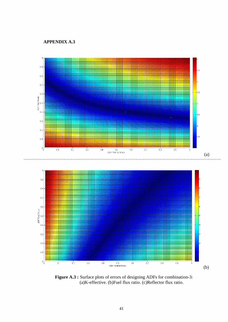
APPENDIX A.3

(a)

(b)


42

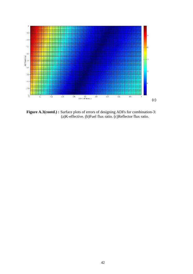
Figure A.3(contd.) : Surface plots of errors of designing ADFs for combination-3:

(a)K-effective. (b)Fuel flux ratio. (c)Reflector flux ratio.

(c)

43

APPENDIX B.1

(a) (b)

(c) (d)

(e) (f)

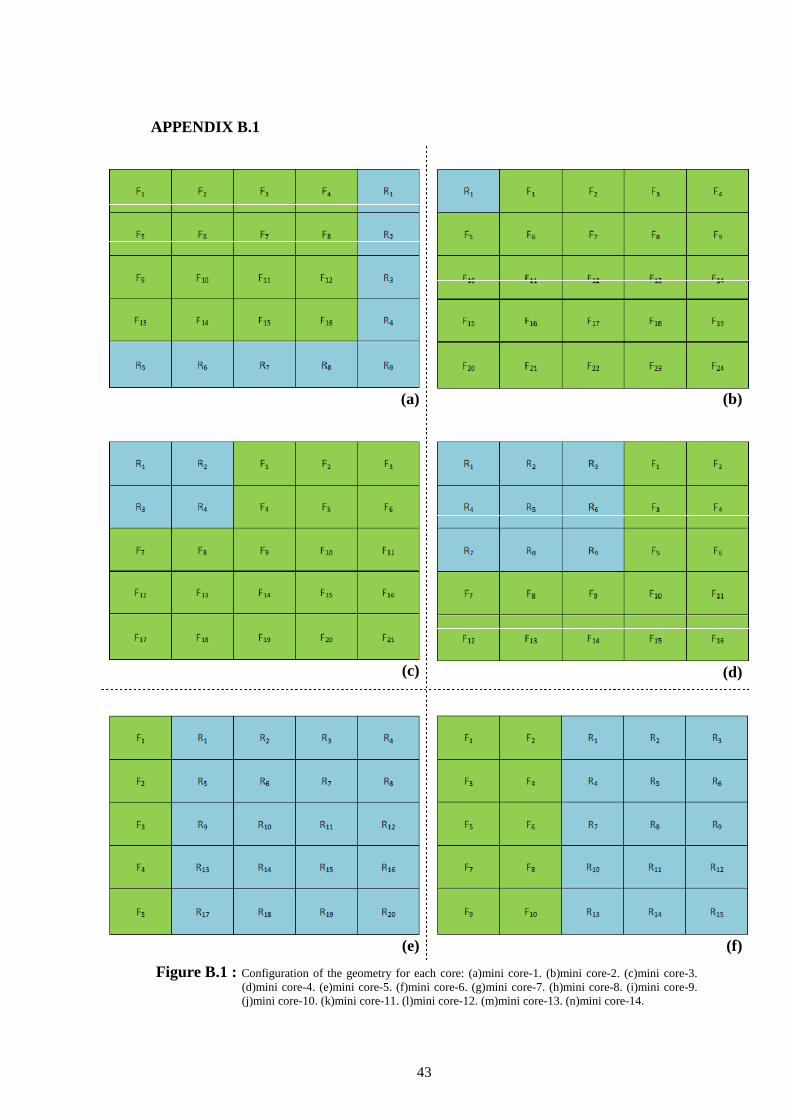
Figure B.1 : Configuration of the geometry for each core: (a)mini core-1. (b)mini core-2. (c)mini core-3. (d)mini core-4. (e)mini core-5. (f)mini core-6. (g)mini core-7. (h)mini core-8. (i)mini core-9. (j)mini core-10. (k)mini core-11. (l)mini core-12. (m)mini core-13. (n)mini core-14.

44

(g) (h)

(i) (j)

(k) (l)

Figure B.1(contd.) : Configuration of the geometry for each core: (a)mini core-1. (b)mini core-2. (c)mini core-3. (d)mini core-4. (e)mini core-5. (f)mini core-6. (g)mini core-7. (h)mini core-8. (i)mini core-9. (j)mini core-10. (k)mini core-11. (l)mini core-12. (m)mini core-13. (n)mini core-14.

45

(m) (n)

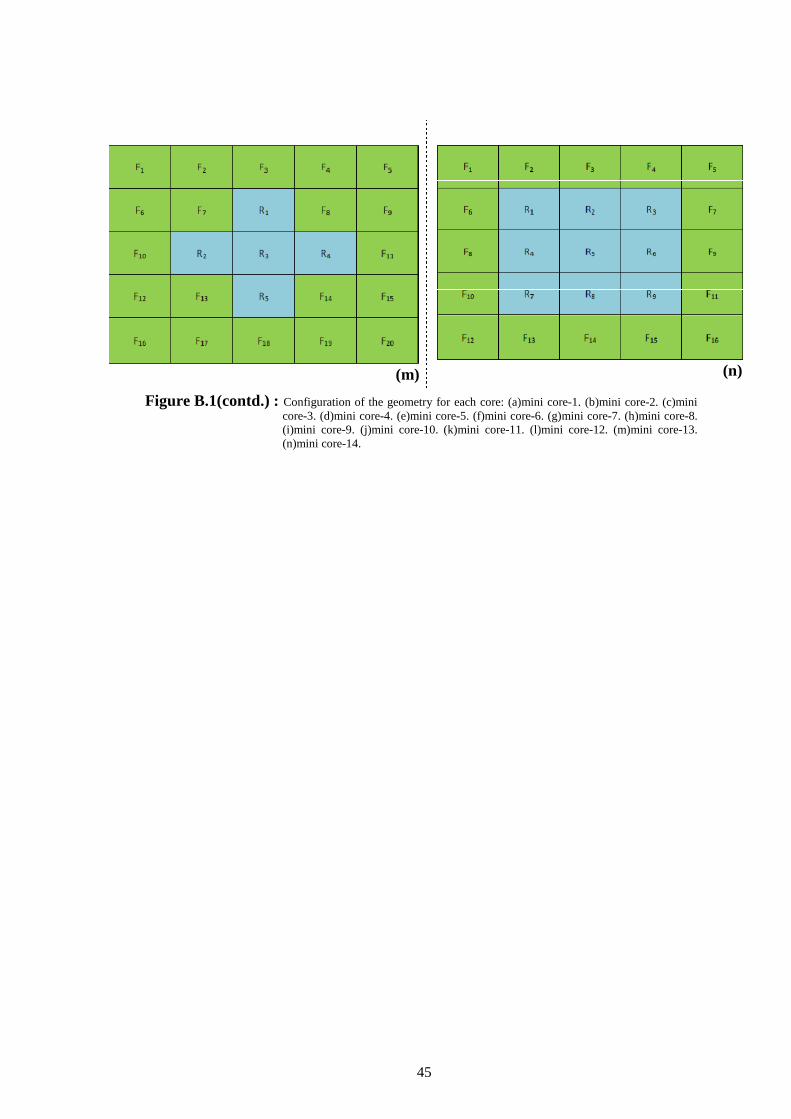
Figure B.1(contd.) : Configuration of the geometry for each core: (a)mini core-1. (b)mini core-2. (c)mini core-3. (d)mini core-4. (e)mini core-5. (f)mini core-6. (g)mini core-7. (h)mini core-8. (i)mini core-9. (j)mini core-10. (k)mini core-11. (l)mini core-12. (m)mini core-13. (n)mini core-14.

CURRICULUM VITA

Candidate’s full name:

Place and date of birth:

Permanent Address:

Universities and Colleges attended:

47

CURRICULUM VITA

Candidate’s full name: Aziz Bora Pekiçten

Place and date of birth: Darmstadt, GERMANY, 5 March 1985

Permanent Address: Hamit Oskay Sok. 5/8, 34730 Göztepe/İST

Colleges attended: Yildiz Technical UniversityIstanbul Technical UniversityRoyal Institute of Technology

Yildiz Technical University Istanbul Technical University Royal Institute of Technology

İSTANBUL TECHNICAL UNIVERSITY ENERGY INSTITUTE …

Documents

Transcript of İSTANBUL TECHNICAL UNIVERSITY ENERGY INSTITUTE …