Stall/Post-Stall Modeling of the Longitudinal Characteristics of a...

AIAA Aviation 2016-3541 13-17 June 2016, Washington, D.C. AIAA Atmospheric Flight Mechanics Conference

Copyright © 2016 by the authors. Published by the American Institute of Aeronautics and Astronautics, Inc., with permission.

Stall/Post-Stall Modeling

of the Longitudinal Characteristics

of a General Aviation Aircraft

Gavin K. Ananda∗ and Michael S. Selig†

Department of Aerospace Engineering, University of Illinois at Urbana–Champaign, Urbana, IL 61801, USA

The high rate of accidents in general aviation due to pilot loss of control has neces-sitated the need to find better methods of training pilots. Pilot control and aware-ness in the stall/post-stall regime can be improved through the use of higher fidelityflight simulators. To create a high fidelity aerodynamic model in the stall/post-stallregime to be implemented in a flight simulator, both steady and unsteady aircraftcharacteristics need to be represented. In this paper, the detailed development of asteady-state high-angle-of-attack general aviation aircraft longitudinal aerodynamicmodel is described. The steady-state model uses a component buildup approachthat uses strip theory to output the aerodynamic forces and moments of an aircraft.An integrated non-linear lifting-line theory approach is used to model the wing andhorizontal tail. Longitudinal effects due to elevator deflections are also included.Validation studies are performed against static wind tunnel datasets for a typicalsingle-engine low-wing general aviation aircraft design.

Nomenclature

A = fuselage cross-sectional areaAb = fuselage base area (at x = l)Ap = fuselage planform area for most casesAr = fuselage reference area (taken as Ab)A = aspect ratiob = wingspanb0 = cross-section widthc = chordCFASF

= fuselage surface skin friction coefficient

cf = flap chordCd = airfoil drag coefficientCdn = crossflow drag coefficient of circular cylinder sectionCD = surface drag coefficient (= D/ 1

2ρV2∞Sref )

Cl = airfoil lift coefficientClα = airfoil lift curve slopeClmax

= airfoil maximum lift coefficientCL = surface lift coefficient (= L/ 1

2ρV2∞Sref )

Cmc/4= airfoil moment coefficient at quarter chord

CMc/4= surface moment coefficient at quarter chord (= M/1

2ρV2∞Srefc)

CN = surface normal force coefficient (= N/ 12ρV

2∞Sref )

Cn = local normal-force coefficient per unit length

∗Graduate Student (Ph.D. Candidate), 104 S. Wright St., AIAA Student Member. [email protected]†Professor, 104 S. Wright St., AIAA Associate Fellow. [email protected]

1 of 26

American Institute of Aeronautics and Astronautics

dF = fuselage cross-section diameterD = dragDind = induced dragk = corner radiuslref = reference lengthlF = fuselage lengthL = liftM = momentnP = number of lifting surface panelsN = normal forcerF = fuselage cross-section radiusRe = Reynolds number based on mean aerodynamic chord (= V∞c/ν)S = lifting surface areaSf = flap areaSref = reference areaV∞ = freestream velocityVF = fuselage volumewind = velocity induced by shed vorticesVrel = relative velocitywF = fuselage widthxF = axial distance from fuselage nosexacF = distance from nose to aerodynamic center of fuselagexcF = distance from nose to centroid of fuselage planform areaxmF

= distance from nose to centroid of fuselage pitching-moment reference centerxPS , yPS , zPS = location of spanwise panel station pointsxLLT , yLLT , zLLT = location of lifting-line pointsY = side forceαeff = effective angle of attackαgeo = geometric angle of attackαind = induced angle of attackβ = sideslip angleδf = flap deflection angleη = flap effectiveness correction factorηfuse = fuselage crossflow drag proportionality factorΓ = circulationΓ0 = circulation at center-spanΓLLT = circulation at the lifting-line pointsΓSV = shed vortex circulationτ = flap effectiveness factorθf = factor relating flap to chord ratio to flap effectiveness factorν = kinematic viscosityρ = density of air

Subscripts

c/4 = quarter-chordcy = cylinderCF = cross-flowF = fuselageNewt = Newtonian theoryo = equivalent circular body of cross sectionSB = slender body

2 of 26


I. Introduction

The need to improve air safety has always been at the forefront of the airline and transportation industry.The Colgan Air 3407 and Air France Flight 447 accidents1,2 that occurred in February and June 2009,respectively, highlighted deficiencies in pilot training with respect to recovering the aircraft from stall andupset states. Furthermore, a recently-concluded 16 year study by Calspan,3 funded mainly by NASA, theFederal Aviation Administration (FAA), and the United States Navy, concluded that pilots were ill-equippedand untrained to recognize an aircraft in an upset state and then perform any appropriate control inputs tosuccessfully recover from this state.

As a result, the FAA and the European Aviation Safety Agency proposed new rules4–6 concerning the useof enhanced Flight Simulation Training Devices (FSTD) for special hazard training such as loss of control.The rulings set a five year mandatory compliance deadline (ending in 2018) to FSTD manufacturers for theproper modeling of stall and upset recovery situations, and that they be valid for at least 10 deg beyond thestall angle of attack. At present, research is being conducted into the improvement of commercial transportaircraft flight modeling and control through the NASA Aviation Safety and Security Program (AvSSP)7–11

and the European Union Simulation and Upset Recovery in Aviation project.12–16

The importance attached to commercial transport aircraft is understandable given that passenger safetyis of the utmost importance to the transportation industry. However, according to the Aircraft Ownersand Pilots Association Air Safety Institute 2010 Nall Report,17 for fixed wing aircraft over the past decade,the average accident rate was 67% higher for non-commercial flights and the rate of fatal accidents was120% higher in comparison with commercial flights. In addition, according to the National Transportationand Safety Board (NTSB) Review of Civil Aviation Accidents from 201018 and the NTSB 2015/2016 MostWanted Transportation Safety Improvements factsheets,19,20 fixed-wing general aviation (GA) accidentsaccounted for 89% of all accidents and 86% of total fatalities of U.S. civil aviation, where loss of controlaccounted for approximately 40% of these fatal accidents. The large proportion of fixed-wing GA aircraftaccidents related to loss of control means that a concerted research effort towards GA aircraft stall/post-stallflight simulation modeling is required. A comprehensive effort similar to the NASA AvSSP program has notyet been pursued. The “Partnership to Enhance General Aviation Safety, Accessibility, and Sustainability”(PEGASAS) program, was recently formed with the goal of enhancing general aviation safety, accesibility,and sustainability.21 However, a review of PEGASAS projects shows that the development of stall/upsetmodeling for the purposes of flight simulation does not fall under its purview.

The use of simulators has been common practice in the past 30 years for pilot training. Simulatorsallow for pilot training in real world situations and are achieved by ensuring that the simulators mimic theaircraft and environment as realistically as possible. The critical limitation common in most simulators isthe lack of fidelity in regimes outside normal flight. One of these limitations relates to aircraft stall. In flightsimulators, stall training for most pilots has been limited to “approach to stall” training, that activates a stallwarning system or stick shaker, upon which recovery is initiated. The primary reason for the lack of fidelityis that most flight simulators are based on stability derivatives that are only accurate in the linear range ofaerodynamic performance. Stall and post-stall effects are highly nonlinear in nature and subsequently arehard to accurately model in real time. A survey of current off-the-shelf flight simulators shows that MicrosoftFlight Simulator X,22 FlightGear,23 and Prepare3D24 all mainly use stability derivatives.

Real-time aerodynamic flight simulation via a physics-based component buildup method using the striptheory approach has more recently been used for flight simulation.25–30 This method has the ability toaccount for non-linear effects associated with the stall regime and will be used in this study. To properlysimulate an aircraft in stall, both steady and unsteady effects need to be modeled.31 This paper will describethe approach taken to model the steady-state longitudinal aerodynamic forces of a typical GA aircraft in thepropeller-off configuration. The approach is validated against a large dataset of experimental wind tunnelresults for a typical single-engine low-wing general aviation design.32 Results from these validations studiesare presented and discussed.

3 of 26


II. Test Case Geometry and Test Conditions

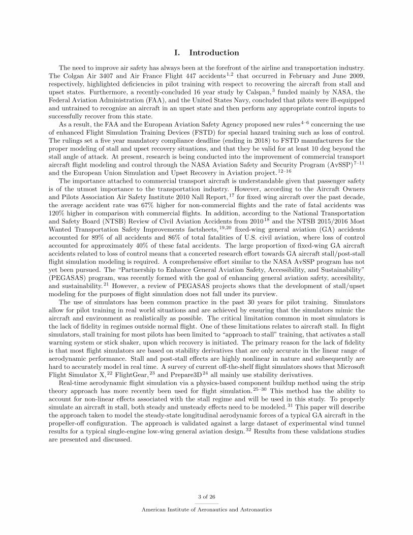
Validation is performed against static wind tunnel test data for a 1/7-scaled and modified version ofa Grumman American AA-1 Yankee (single-engine, low-wing GA model).32 The wind tunnel tests wereperformed as part of the NASA Stall/Spin Project carried out in the 1970-80s.33 The low-wing generalaviation (LWGA) aircraft is modeled using OpenVSP34,35 and exported to SolidWorks based on three-viewsand dimensional characteristics of the model.32,36 An isometric view of the wireframe mesh and surfacedmodel is shown in Fig. 1.

The 1/7-th scale LWGA model has a rectangular wing with a 0.5725 ft chord and 3.5 ft span. The winghas a dihedral of 5 deg and is set at an incidence angle (iW ) of 3.5 deg with no geometric twist. The spanof the horizontal tail is 1.07 ft, and it is set at an incidence angle (iHT ) of −3 deg. The horizontal tailnumber referenced in Table 1 relates to the vertical location of the horizontal tail with respect to the aircraftcenterline. Horizontal tail #3 is located 0.0917 ft above the aircraft centerline, and its root leading edge isaligned with the root leading edge of the vertical tail.

Wind tunnel tests were conducted at a Mach number of 0.2 at Reynolds numbers of 0.288×106 and3.45×106. Test datasets include full aircraft and individual component force and moment coefficients forangles of attack from −8 to 90 deg and sideslip angles from −10 to 30 deg. In addition, datasets characterizingaerodynamic effects of the aircraft due to elevator, aileron, and rudder deflections are also available. Thedatasets from Ref. 32 are for a propeller-off configuration. For the current study, only longitudinal aircraftcharacteristics (CL, CD, and CMcg) at a Reynolds number of 3.45×106 were modeled. The higher Reynoldsnumber case was chosen as it was a closer representation to the full-scale aircraft. The pitching momentresults are presented based on the LWGA aircraft center-of-gravity position of 0.255c. Table 1 lists thevarious LWGA aircraft configurations that the longitudinal aerodynamic model will be validated against.

Figure 1. Isometric view of the LWGA model.

Table 1. Low-Wing General Aviation Aircraft Configurations Tested

Configurationδe

[deg]δa

[deg]δr

[deg]B 0 0 0BW1 0 0 0BH3 0 0 0BV 0 0 0BW1H3 0 0 0BW1H3V 0 0 0BW1H3V −25 0 0BW1H3V 15 0 0

B: Fuselage

H3: Horizontal tail #3

W1: Modified NACA 642 - 415 airfoil

V: Vertical Tail

4 of 26


III. Modeling Methodology

The goal of modeling a single-engine GA for stall/upset events is a challenging endeavor given the numberof effects that need to be accurately modeled throughout the entire flight envelope. A variety of modelingmethods have been used (i.e., stability derivative methods, full aerodynamic lookup tables, etc.). The mostrobust method, albeit with lower fidelity, that has been employed is a physics-based component-buildupmethod using the strip theory approach.

In the component-buildup approach, an airplane is separated into its main individual components: pro-peller, wing, fuselage, horizontal tail, and vertical tail. Each component (apart from the propeller) is thenmodeled using a strip-theory approach in which individual components are further subdivided into sections.Each of these sections are then subjected to varying local relative flow that is based on aircraft speed, in-duced flow, kinematics, wind, propeller slipstream, and other interference effects. For the current study, onlyaircraft speed and induced flow due to shed vortices is considered. Data tables for each of the componentsections are derived from wind tunnel results, computational fluid dynamics (CFD) runs, numerical panelmethods, and/or semi-empirical methods.The methodology involved in development of each of these datatables will be further discussed in the following subsections.

An integrated non-linear lifting-line theory25,26,37,38 approach is then used to determine the local inducedangle of attack at each strip of the wing and horizontal tail. This method has the ability to account forthe effect of individual surface deflection angles and most importantly non-linear effects associated with thestall regime. Components and effects that will contribute to the lateral characteristics of the aircraft (i.e.,vertical tail and wake shielding) are not included as only longitudinal aircraft characteristics are modeled inthis study.

A. Airfoil Model

The proper modeling of the aerodynamic performance of airfoils for the wing and horizontal tail is theprimary factor that determines the static-stall characteristics of an aircraft. The magnitude of airfoil Clmax

directly relates to the aircraft flight speed and angle of attack. Consequently, Clmaxdetermines the takeoff,

approach, and landing characteristics of an aircraft. Thus, for increased simulation fidelity, it is crucial thatthe stall characteristics of an airfoil (Clmax

, αstall, type of stall, etc.) is accurately predicted.

Broadly, there are four approaches to predicting steady-state airfoil performance: wind tunnel testing,computational fluid dynamics (CFD) simulations, numerical panel methods (e.g., XFOIL39), empirical, andsemi-empirical methods that use some combination of the previous four methods. Wind tunnel tests are thecurrent main source of accurate airfoil performance data. Airfoil performance data in the pre-stall regime upto stall are widely available both at low40–45 (Re ≤ 500,000) and high46 (Re > 500,000) Reynolds numbers.In the post-stall regime, however, only a sparse amount of wind tunnel test data is available.47–50 In itscurrent state-of-the-art, CFD is used as an ideal tool for design and optimization studies. In addition,it is used to better understand flow behavior around objects. CFD methods, however, still suffer due tothe inability to deal with highly separated flows that are typical for a wing in the post-stall regime.51

In addition, building an accurate set of lookup tables for flight simulation would take prohibitively longeven using Reynolds-Averaged Navier Stokes (RANS) CFD simulations. For this study, the authors didnot use CFD in the aerodynamic modeling. Instead, numerical panel method codes (with boundary layerintegration) such as XFOIL are fast and accurate pre-stall. However, XFOIL is known to overpredict Clmax

and underpredict minimum drag.52 The best approach to modeling airfoil performance both pre-stall andpost-stall is some combination of the previous three methods together with validated empirical models (i.e.,AERODAS model53).

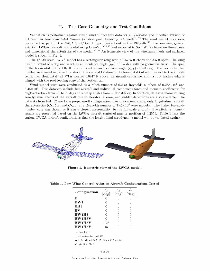
The LWGA wing has a rectangular planform and uses a ‘modified’ NACA 642-415 airfoil section.36 Itshorizontal and vertical tail both use the NACA 651-012 airfoil sections. A coplot of the original NACA642-415 airfoil against the ‘modified’ airfoil section is shown in Fig. 2. The difference between the originaland modified NACA 642-415 airfoils is the amount of aft camber and trailing edge thickness.

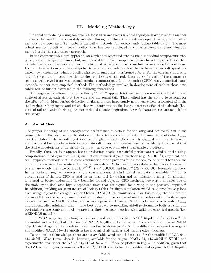
To the authors’ knowledge, there are no available wind tunnel data sets for the modified NACA 642-415 airfoil. Wind tunnel data is, however, available for the original NACA 642-415 airfoil.46 XFOIL andexperimental results for the NACA 642-415 at Re = 3×106 are co-plotted in Fig. 3. In addition, given thatthe LWGA test Reynolds number is 3.45×106, XFOIL results for the modified and original NACA 642-415

5 of 26


0 0.1 0.2 0.3 0.4 0.5 0.6 0.7 0.8 0.9 1−0.1

0

0.1

0.2

0.3

x

y

NACA 64

2−415 MOD

NACA 642−415

Figure 2. Comparison of original and modified NACA 642-415 airfoils.

−50 −40 −30 −20 −10 0 10 20 30 40 50−1.5

−1

−0.5

0

0.5

1

1.5

2

α (deg)

Cl

NACA 642−415 MOD Re=3.45x106 XFOIL

NACA 642−415 Re=3.45x106 XFOIL

NACA 642−415 Re=3x106 XFOIL

NACA 642−415 Re=3x106 EXP [46]

(a)

−50 −40 −30 −20 −10 0 10 20 30 40 500

0.05

0.1

0.15

0.2

0.25

0.3

0.35

0.4

0.45

0.5

α (deg)

Cd

NACA 642−415 MOD Re=3.45x106 XFOIL



NACA 642−415 Re=3x106 EXP [46]

(b)

−50 −40 −30 −20 −10 0 10 20 30 40 50−0.2

−0.15

−0.1

−0.05

0

0.05

0.1

0.15

0.2

α (deg)

Cm

c4

NACA 64

2−415 MOD Re=3.45x106 XFOIL



NACA 642−415 Re=3x106 EXP [46]

(c)

Figure 3. XFOIL and experimental aerodynamic data for NACA 642-415 modified and baseline airfoil (a) liftcurve, (b) drag polars, and (c) moment curves.

airfoil at Re = 3.45×106 are coplotted. Comparing the XFOIL results for the two airfoils at Re = 3.45×106,it is evident that the reduction in aft camber in the modified airfoil reduces its Clmax

and pitch down

6 of 26


−0.2 0 0.2 0.4 0.6 0.8 1 1.2−0.1

0

0.1

0.2

0.3

0.4

x

y

NACA 64

2−415 MOD

NACA 642−415

NACA 643−618

GA(W)−1

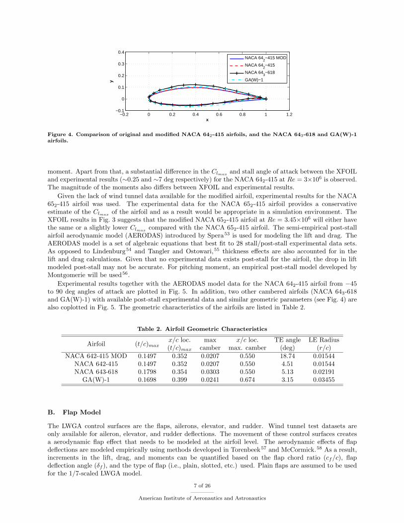
Figure 4. Comparison of original and modified NACA 642-415 airfoils, and the NACA 643-618 and GA(W)-1airfoils.

moment. Apart from that, a substantial difference in the Clmax and stall angle of attack between the XFOILand experimental results (∼0.25 and ∼7 deg respectively) for the NACA 642-415 at Re = 3×106 is observed.The magnitude of the moments also differs between XFOIL and experimental results.

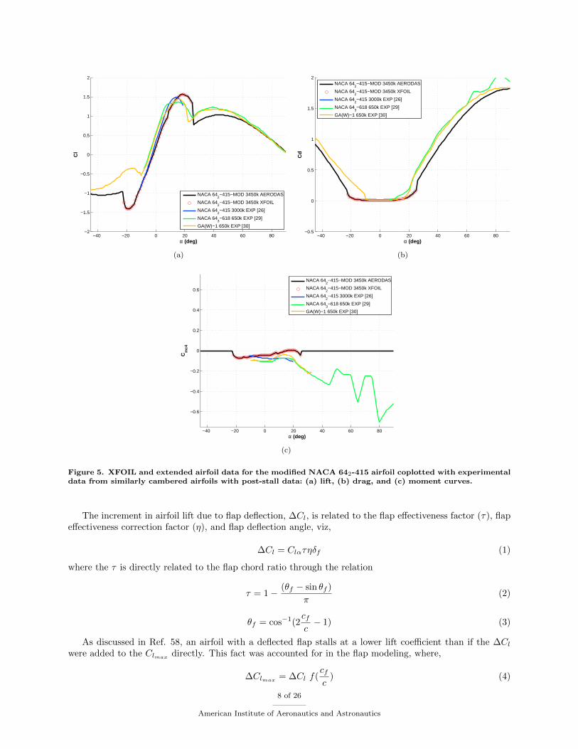
Given the lack of wind tunnel data available for the modified airfoil, experimental results for the NACA652-415 airfoil was used. The experimental data for the NACA 652-415 airfoil provides a conservativeestimate of the Clmax of the airfoil and as a result would be appropriate in a simulation environment. TheXFOIL results in Fig. 3 suggests that the modified NACA 652-415 airfoil at Re = 3.45×106 will either havethe same or a slightly lower Clmax

compared with the NACA 652-415 airfoil. The semi-empirical post-stallairfoil aerodynamic model (AERODAS) introduced by Spera53 is used for modeling the lift and drag. TheAERODAS model is a set of algebraic equations that best fit to 28 stall/post-stall experimental data sets.As opposed to Lindenburg54 and Tangler and Ostowari,55 thickness effects are also accounted for in thelift and drag calculations. Given that no experimental data exists post-stall for the airfoil, the drop in liftmodeled post-stall may not be accurate. For pitching moment, an empirical post-stall model developed byMontgomerie will be used56.

Experimental results together with the AERODAS model data for the NACA 642-415 airfoil from −45to 90 deg angles of attack are plotted in Fig. 5. In addition, two other cambered airfoils (NACA 643-618and GA(W)-1) with available post-stall experimental data and similar geometric parameters (see Fig. 4) arealso coplotted in Fig. 5. The geometric characteristics of the airfoils are listed in Table 2.

Table 2. Airfoil Geometric Characteristics

Airfoil (t/c)maxx/c loc.(t/c)max

maxcamber

x/c loc.max. camber

TE angle(deg)

LE Radius(r/c)

NACA 642-415 MOD 0.1497 0.352 0.0207 0.550 18.74 0.01544NACA 642-415 0.1497 0.352 0.0207 0.550 4.51 0.01544NACA 643-618 0.1798 0.354 0.0303 0.550 5.13 0.02191

GA(W)-1 0.1698 0.399 0.0241 0.674 3.15 0.03455

B. Flap Model

The LWGA control surfaces are the flaps, ailerons, elevator, and rudder. Wind tunnel test datasets areonly available for aileron, elevator, and rudder deflections. The movement of these control surfaces createsa aerodynamic flap effect that needs to be modeled at the airfoil level. The aerodynamic effects of flapdeflections are modeled empirically using methods developed in Torenbeek57 and McCormick.58 As a result,increments in the lift, drag, and moments can be quantified based on the flap chord ratio (cf/c), flapdeflection angle (δf ), and the type of flap (i.e., plain, slotted, etc.) used. Plain flaps are assumed to be usedfor the 1/7-scaled LWGA model.

7 of 26


−40 −20 0 20 40 60 80−2

−1.5

−1

−0.5

0

0.5

1

1.5

2

α (deg)

Cl

NACA 642−415−MOD 3450k AERODAS

NACA 642−415−MOD 3450k XFOIL

NACA 642−415 3000k EXP [26]

NACA 643−618 650k EXP [29]

GA(W)−1 650k EXP [30]

(a)

−40 −20 0 20 40 60 80−0.5

0

0.5

1

1.5

2

α (deg)

Cd

NACA 64

2−415−MOD 3450k AERODAS


NACA 642−415 3000k EXP [26]

NACA 643−618 650k EXP [29]

GA(W)−1 650k EXP [30]

(b)

−40 −20 0 20 40 60 80

−0.6

−0.4

−0.2

0

0.2

0.4

0.6

α (deg)

Cm

c4

NACA 64

2−415−MOD 3450k AERODAS


NACA 642−415 3000k EXP [26]

NACA 643−618 650k EXP [29]

GA(W)−1 650k EXP [30]

(c)

Figure 5. XFOIL and extended airfoil data for the modified NACA 642-415 airfoil coplotted with experimentaldata from similarly cambered airfoils with post-stall data: (a) lift, (b) drag, and (c) moment curves.

The increment in airfoil lift due to flap deflection, ∆Cl, is related to the flap effectiveness factor (τ), flapeffectiveness correction factor (η), and flap deflection angle, viz,

∆Cl = Clατηδf (1)

where the τ is directly related to the flap chord ratio through the relation

τ = 1 − (θf − sin θf )

π(2)

θf = cos−1(2cfc

− 1) (3)

As discussed in Ref. 58, an airfoil with a deflected flap stalls at a lower lift coefficient than if the ∆Clwere added to the Clmax

directly. This fact was accounted for in the flap modeling, where,

∆Clmax= ∆Cl f(

cfc

) (4)

8 of 26


The increment of lifting surface drag, ∆CD, due to flap deflection is related to the flap chord ratio, flaparea to surface area ratio (

Sf

S ), and flap deflection angle is given by the relation

∆CD = 1.7(cf/c)1.38(Sf/S) sin2 δf (5)

The moment increment, ∆Cm,c/4, is related to the ∆Cl based on thin airfoil theory. Similar to an airfoilwith camber, the airfoil is treated as a flat plate with a flap deflected yielding

∆Cm,c/4 = −∆Cl2 sin θf − sin 2θf8(π − θf + sin θf )

(6)

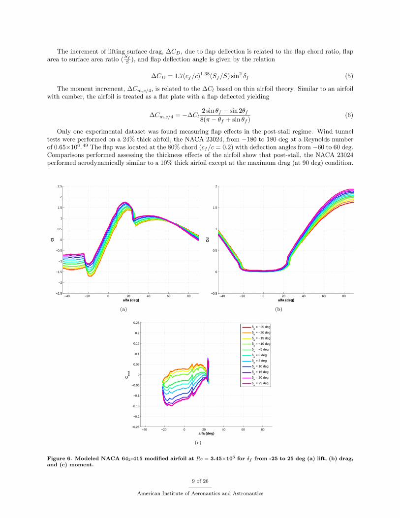
Only one experimental dataset was found measuring flap effects in the post-stall regime. Wind tunneltests were performed on a 24% thick airfoil, the NACA 23024, from −180 to 180 deg at a Reynolds numberof 0.65×106.49 The flap was located at the 80% chord (cf/c = 0.2) with deflection angles from −60 to 60 deg.Comparisons performed assessing the thickness effects of the airfoil show that post-stall, the NACA 23024performed aerodynamically similar to a 10% thick airfoil except at the maximum drag (at 90 deg) condition.

−40 −20 0 20 40 60 80−2.5

−2

−1.5

−1

−0.5

0

0.5

1

1.5

2

2.5

alfa (deg)

Cl

(a)

−40 −20 0 20 40 60 80−0.5

0

0.5

1

1.5

2

alfa (deg)

Cd

(b)

−40 −20 0 20 40 60 80−0.25

−0.2

−0.15

−0.1

−0.05

0

0.05

0.1

0.15

0.2

0.25

alfa (deg)

Cm

c4

δa = −25 deg

δa = −20 deg

δa = −15 deg

δa = −10 deg

δa = −5 deg

δa = 0 deg

δa = 5 deg

δa = 10 deg

δa = 15 deg

δa = 20 deg

δa = 25 deg

(c)

Figure 6. Modeled NACA 642-415 modified airfoil at Re = 3.45×106 for δf from -25 to 25 deg (a) lift, (b) drag,and (c) moment.

9 of 26


This means that observations can be taken with sufficient confidence and applied to thinner airfoils. Themain observations from the wind tunnel results are the flap effects close to 90 deg. Given that with varyingflap deflection, the effective chordline of the airfoil changes, this means that the location of zero lift varieswith flap deflection. In addition, the drag coefficient directly relates to the direction of flap deflection. Lift,drag, and pitching moment curves for the wing airfoil for δf from −25 to 25 deg are plotted in Fig. 6. As asanity check for the post-stall drag results, it can be imagined that with a positive flap angle (trailing edgedown) at high angles of attack, the airfoil would act like a scoop thereby causing an increase in maximumdrag as observed in Fig. 6.

C. Lifting Surface Model (Wing / Horizontal Tail)

An integrated non-linear lifting-line model is used for real-time calculation of the wing and horizontal tailaerodynamics from the airfoil data as required for flight simulation. The method uses lookup tables generatedfor the airfoil at different angles of attack and flap angles and has been used in research37,38,59,60 andcommercially28,30 for real-time flight simulation. In the current approach, the influence of the various liftingsurfaces on each other are considered. Note that external flow effects (i.e. slipstream effects and wakeshielding) are not modeled. The non-linear lifting line calculation methodology is detailed as follows.

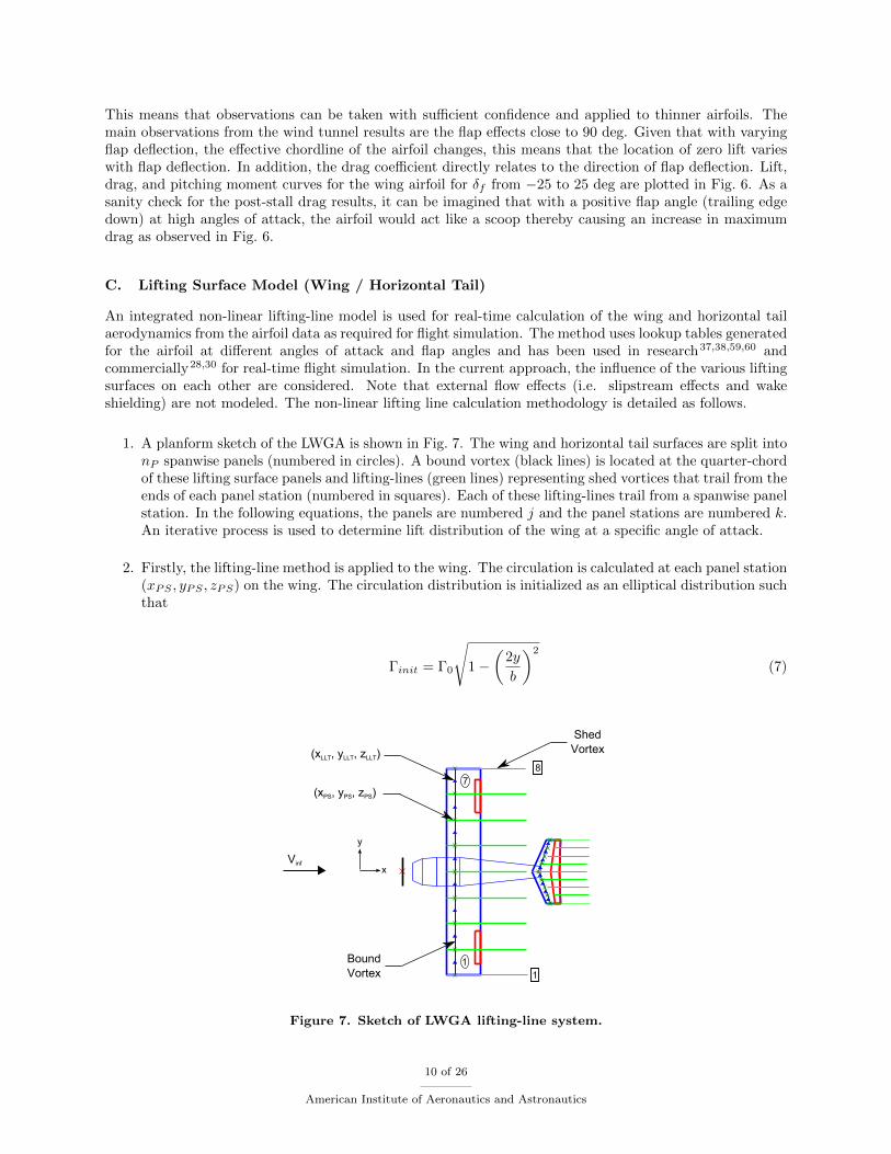
1. A planform sketch of the LWGA is shown in Fig. 7. The wing and horizontal tail surfaces are split intonP spanwise panels (numbered in circles). A bound vortex (black lines) is located at the quarter-chordof these lifting surface panels and lifting-lines (green lines) representing shed vortices that trail from theends of each panel station (numbered in squares). Each of these lifting-lines trail from a spanwise panelstation. In the following equations, the panels are numbered j and the panel stations are numbered k.An iterative process is used to determine lift distribution of the wing at a specific angle of attack.

2. Firstly, the lifting-line method is applied to the wing. The circulation is calculated at each panel station(xPS , yPS , zPS) on the wing. The circulation distribution is initialized as an elliptical distribution suchthat

Γinit = Γ0

√1 −

(2y

b

)2

(7)

Vinf

Bound

Vortex

Shed

Vortex(xLLT, yLLT, zLLT)

(xPS, yPS, zPS)

1

8

1

7

x

y

Figure 7. Sketch of LWGA lifting-line system.

10 of 26


where the circulation at the center span, Γ0, is calculated from Kutta-Joukowski Theorem given by

Γ0 =1

2V∞crootCl (8)

The sectional Cl is based on the effective angle of attack (αeff ) and δf at each station where

αeff = αgeo − αind + isurface (9)

The induced angle of attack, αind, is set to 0 for the first iteration.

3. The circulation is then calculated at each lifting-line point (xLLT , yLLT , zLLT ). The lifting-line points(blue triangles) are located on the bound vortex at the center of each lifting surface panel. Thecirculation at each lifting line point is given by

ΓLLTj=

Γinitj + Γinitj+1

2(10)

4. The vorticity shed at each spanwise panel station is then calculated using

ΓSV1= ΓLLT1

(11)

ΓSVnP= ΓLLTnP

(12)

ΓSVj= ΓLLTj

− ΓLLTj−1(13)

5. Next, the induced velocity at each lifting-line point is calculated due to each trailing vortex. Thisis done via an extension of the Biot-Savart law.61 The velocity induced by a shed vortex located atspanwise panel station, k, on the lifting-line point, j, is given by

windjk =ΓSVk

4π

(yPSk

− yLLTj

(zLLTj − zPSk)2 + (yLLTj − yPSk

)2

)[

1.0 +xLLTj

− xPSk√(xLLTj − xPSk

)2 + (yLLTj − yPSk)2 + (zLLTj − zPSk

)2

] (14)

The total velocity induced at each lifting-line point, j, due to the shed vortices is then summed, viz

windj =

nP+1∑k=1

windjk (15)

6. Once the induced velocity at each lifting-line point is calculated, the new induced angle of attackrelative to the airfoil chordline at each lifting-line point is calculated as

αindj = tan−1(−windj

V∞

)(16)

7. The sectional lift coefficient Cl is interpolated from airfoil lookup tables based on the new αeffj(calculated using Eq. 9) and δfj at each lifting-line point.

8. The induced velocity due to the shed vortices requires for the calculation of a new relative velocity ateach lifting line point, that is

Vrelj =√V∞

2 + windj2 (17)

11 of 26


9. The direction of the relative velocity causes a normal force that has a lift and induced drag componentgiven by

N ′j =L′j

cos(αindj )(18)

and

N ′j = ρVreljΓLLTj(19)

resulting in the calculation of the new circulation distribution at the lifting-line point that is

ΓLLT,newj=

1

2

V 2∞

Vrelj

1

cos(αindj )cjClj(20)

The chord is based on the chordwise distribution over the wing. For the LWGA wing, the chordwisedistribution is constant.

10. The circulation distribution to be used for the next iteration is a combination of the previous circu-lation together with the newly calculated circulation distribution. Anderson38 suggests the followingequation, where D is the damping factor for the iterations

ΓLLTj= DΓLLT,newj

+ (1 −D)ΓLLTj(21)

A damping factor D of 0.05 to 0.1 is used.

11. Steps 4–10 are repeated until a criteria for convergence is satified. The convergence criteria is given by

∑nP

j=1(ΓLLT,newj− ΓLLTj

)2

nP≤ 0.00001 (22)

12. Once convergence is satisfied, the total lift for the wing is determined by summing the lift contributionsof the individual panels of the wing. Induced drag is also similarly calculated using

L =

nP∑j=1

ρVreljΓLLTj cos(αindj )∆ypanelj (23)

Dind =

nP∑j=1

ρVreljΓLLTj sin(αindj )∆ypanelj (24)

The profile drag and pitching moment of the lifting surface are calculated by summing the individualsection contributions. This method ensures that control surface deflections and other effects local to a specifcpanel section are included in the overall calculation. The total drag for the lifting surface is calculated bysumming the profile drag and induced drag contributions. For the current study, each lifting surface is splitinto 30 panel sections and requires 100-200 iterations to converge.

12 of 26


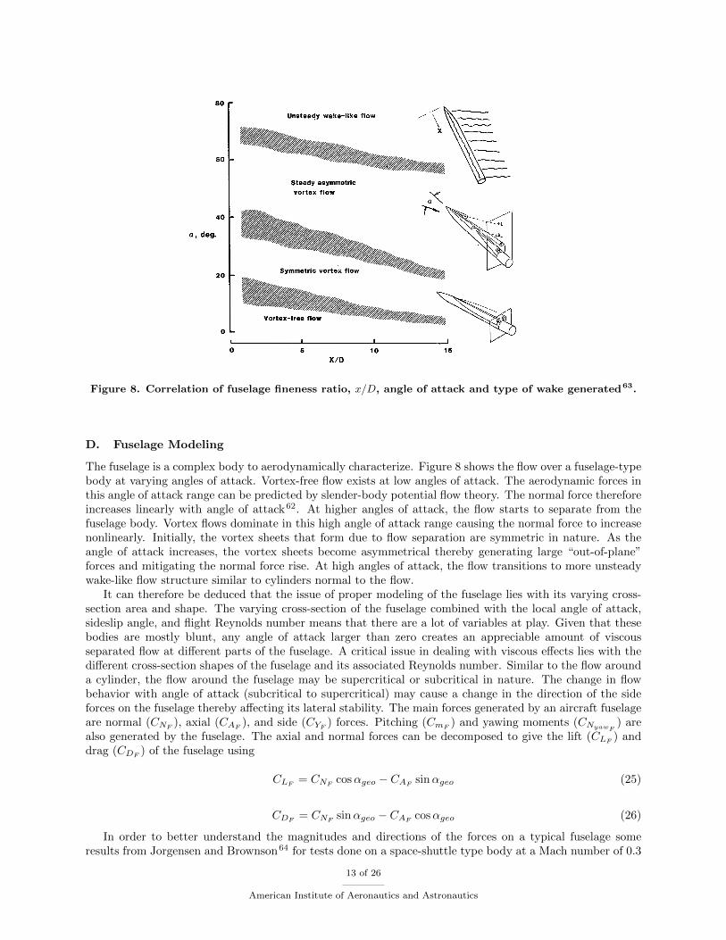
Figure 8. Correlation of fuselage fineness ratio, x/D, angle of attack and type of wake generated63.

D. Fuselage Modeling

The fuselage is a complex body to aerodynamically characterize. Figure 8 shows the flow over a fuselage-typebody at varying angles of attack. Vortex-free flow exists at low angles of attack. The aerodynamic forces inthis angle of attack range can be predicted by slender-body potential flow theory. The normal force thereforeincreases linearly with angle of attack62. At higher angles of attack, the flow starts to separate from thefuselage body. Vortex flows dominate in this high angle of attack range causing the normal force to increasenonlinearly. Initially, the vortex sheets that form due to flow separation are symmetric in nature. As theangle of attack increases, the vortex sheets become asymmetrical thereby generating large “out-of-plane”forces and mitigating the normal force rise. At high angles of attack, the flow transitions to more unsteadywake-like flow structure similar to cylinders normal to the flow.

It can therefore be deduced that the issue of proper modeling of the fuselage lies with its varying cross-section area and shape. The varying cross-section of the fuselage combined with the local angle of attack,sideslip angle, and flight Reynolds number means that there are a lot of variables at play. Given that thesebodies are mostly blunt, any angle of attack larger than zero creates an appreciable amount of viscousseparated flow at different parts of the fuselage. A critical issue in dealing with viscous effects lies with thedifferent cross-section shapes of the fuselage and its associated Reynolds number. Similar to the flow arounda cylinder, the flow around the fuselage may be supercritical or subcritical in nature. The change in flowbehavior with angle of attack (subcritical to supercritical) may cause a change in the direction of the sideforces on the fuselage thereby affecting its lateral stability. The main forces generated by an aircraft fuselageare normal (CNF

), axial (CAF), and side (CYF

) forces. Pitching (CmF) and yawing moments (CNyawF

) arealso generated by the fuselage. The axial and normal forces can be decomposed to give the lift (CLF

) anddrag (CDF

) of the fuselage using

CLF= CNF

cosαgeo − CAFsinαgeo (25)

CDF= CNF

sinαgeo − CAFcosαgeo (26)

In order to better understand the magnitudes and directions of the forces on a typical fuselage someresults from Jorgensen and Brownson64 for tests done on a space-shuttle type body at a Mach number of 0.3

13 of 26


(a) (b)

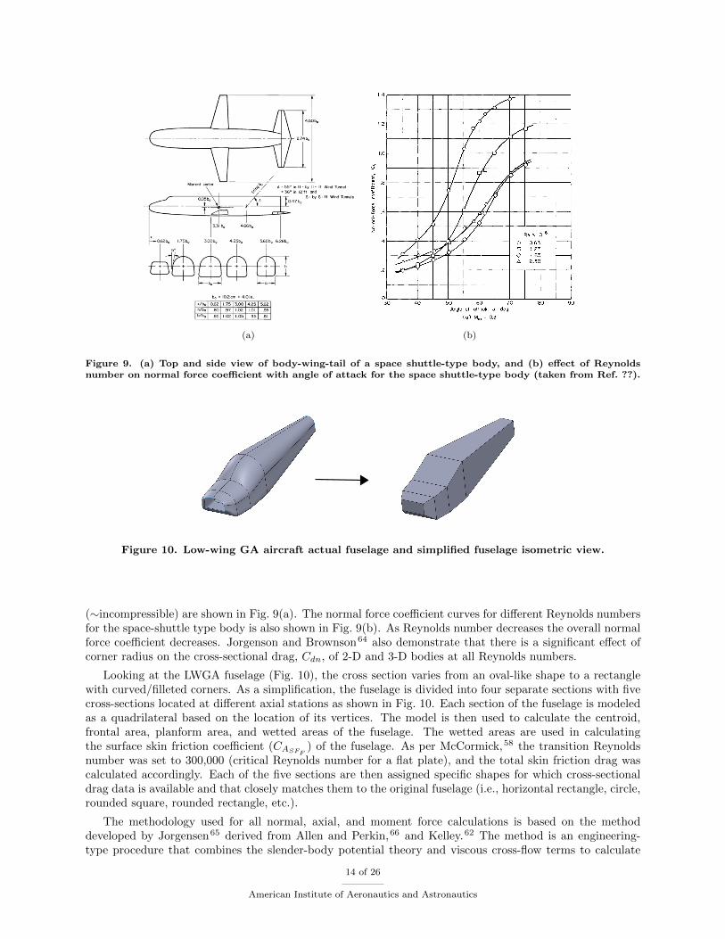
Figure 9. (a) Top and side view of body-wing-tail of a space shuttle-type body, and (b) effect of Reynoldsnumber on normal force coefficient with angle of attack for the space shuttle-type body (taken from Ref. ??).

Figure 10. Low-wing GA aircraft actual fuselage and simplified fuselage isometric view.

(∼incompressible) are shown in Fig. 9(a). The normal force coefficient curves for different Reynolds numbersfor the space-shuttle type body is also shown in Fig. 9(b). As Reynolds number decreases the overall normalforce coefficient decreases. Jorgenson and Brownson64 also demonstrate that there is a significant effect ofcorner radius on the cross-sectional drag, Cdn, of 2-D and 3-D bodies at all Reynolds numbers.

Looking at the LWGA fuselage (Fig. 10), the cross section varies from an oval-like shape to a rectanglewith curved/filleted corners. As a simplification, the fuselage is divided into four separate sections with fivecross-sections located at different axial stations as shown in Fig. 10. Each section of the fuselage is modeledas a quadrilateral based on the location of its vertices. The model is then used to calculate the centroid,frontal area, planform area, and wetted areas of the fuselage. The wetted areas are used in calculatingthe surface skin friction coefficient (CASFF

) of the fuselage. As per McCormick,58 the transition Reynoldsnumber was set to 300,000 (critical Reynolds number for a flat plate), and the total skin friction drag wascalculated accordingly. Each of the five sections are then assigned specific shapes for which cross-sectionaldrag data is available and that closely matches them to the original fuselage (i.e., horizontal rectangle, circle,rounded square, rounded rectangle, etc.).

The methodology used for all normal, axial, and moment force calculations is based on the methoddeveloped by Jorgensen65 derived from Allen and Perkin,66 and Kelley.62 The method is an engineering-type procedure that combines the slender-body potential theory and viscous cross-flow terms to calculate

14 of 26


the normal force and pitching moment by way of

CNF= CNSBF

+ CNCFF(27)

CmF= CmSBF

+ CmCFF(28)

where the slender body (SB) potential theory terms are given by

CNSBF=

(AbAr

)sin(2α) cos

(α2

)( CnCn0

)SBave

cosβ (29)

CMSBF= −

[(VF −AbxmArdeq

)sin(2α) cos

(α2

)]( CnCn0

)SBave

cosβ (30)

The term(Cn

Cn0

)SBave

is a ratio that varies from 1.19 at k = 0 (no corner radius) to 1.00 at k = 0.5

(completely circular cross section). The term is also averaged from the four separate sections. The cosβterm is included to correct for sideslip effects. The equivalent diameter (deq) is calculated based on the width(b0) and corner radius (k) of the square or rectangular cross section using

deq = 2b0

√1 − (4 − π)k2

π(31)

where

k =r

b0(32)

The crossflow terms for normal force and pitching moment are given by

CNCFF=NCFF

qAr=ηF sin2(α)

Ar

∫ l

0

b0Cdnb0deq

dx (33)

CmCFF=NCFF

qArc=η sin2(α)

Ardeq

∫ l

0

b0Cdnb0deq

(xm − xc)dx (34)

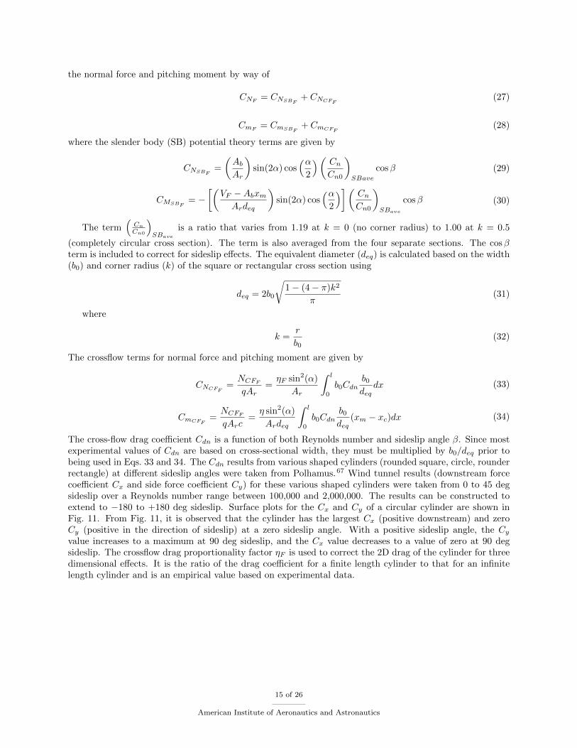
The cross-flow drag coefficient Cdn is a function of both Reynolds number and sideslip angle β. Since mostexperimental values of Cdn are based on cross-sectional width, they must be multiplied by b0/deq prior tobeing used in Eqs. 33 and 34. The Cdn results from various shaped cylinders (rounded square, circle, rounderrectangle) at different sideslip angles were taken from Polhamus.67 Wind tunnel results (downstream forcecoefficient Cx and side force coefficient Cy) for these various shaped cylinders were taken from 0 to 45 degsideslip over a Reynolds number range between 100,000 and 2,000,000. The results can be constructed toextend to −180 to +180 deg sideslip. Surface plots for the Cx and Cy of a circular cylinder are shown inFig. 11. From Fig. 11, it is observed that the cylinder has the largest Cx (positive downstream) and zeroCy (positive in the direction of sideslip) at a zero sideslip angle. With a positive sideslip angle, the Cyvalue increases to a maximum at 90 deg sideslip, and the Cx value decreases to a value of zero at 90 degsideslip. The crossflow drag proportionality factor ηF is used to correct the 2D drag of the cylinder for threedimensional effects. It is the ratio of the drag coefficient for a finite length cylinder to that for an infinitelength cylinder and is an empirical value based on experimental data.

15 of 26


(a) (b)

Figure 11. Forces on a cylinder as a function of Reynolds number and sideslip angle: (a) CX , (b) CY .

16 of 26


IV. Results and Discussion

The methods discussed in Sec. III detail the aerodynamic modeling of the longitudinal characteristicsof the aircraft in the propeller-off state. The current section presents results of the developed aerodynamicmodel for the chosen low-wing General Aviation aircraft. The longitudinal aerodynamics (CL, CD, andCMcg) results of the model will be presented with wind tunnel results at a Reynolds number of 3.45 × 106.All results are non-dimensionalized by the LWGA wing area and results are presented for angles of attackfrom −10 to 40 deg. Pitching moment results are presented based on the LWGA aircraft center-of-gravityposition of 0.255c. The configurations mainly compared are as detailed in Table 1. All lift, drag, and pitchingmoment coefficient plot limits are maintained the same to facilitate easier comparison between the differentsets of results presented.

A. Fuselage Only

As decribed in Section III.D, the fuselage of the LWGA is first divided into four separate sections withquadrilateral cross-sections assigned to a shape with known cross-sectional data. Cross-section data to beused in the fuselage modeling calculations are taken from Ref. 63. Given that only longitudinal characteristicsare modeled, the zero sideslip cases are only required and the side force effects are ignored.

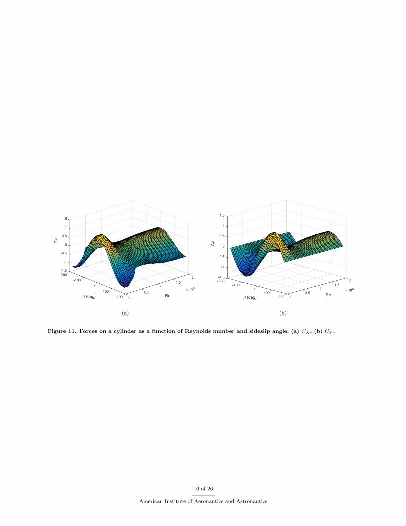
The calculated lift, drag and pitching moment coefficients for the fuselage are coplotted together withwind tunnel results from Ref. 32 in Fig. 12. From the results, the calculated lift and drag coefficients of

−10 −5 0 5 10 15 20 25 30 35 40−1.5

−1

−0.5

0

0.5

1

1.5

2

α (deg)

CL

Fuselage ModelBihrle et al., 1978 [26]

(a)

−10 −5 0 5 10 15 20 25 30 35 400

0.1

0.2

0.3

0.4

0.5

0.6

0.7

0.8

α (deg)

CD


(b)

−10 −5 0 5 10 15 20 25 30 35 40−1

−0.8

−0.6

−0.4

−0.2

0

0.2

0.4

0.6

0.8

1

α (deg)

CM

cg


(c)

Figure 12. (a) Lift, (b) drag, and (c) pitching moment coefficients of LWGA fuselage at Re of 3.45×106.

17 of 26


the fuselage align well with the wind tunnel results at low angles of attack (α ≤ 20 deg). The resultsdeviate however, at high angles of attack with the model underpredicting both lift and drag coefficients. Thepitching moment results for the fuselage also do not match with the validation data. According to Jorgensenand Brownson,64 the pitching moment of the fuselage should be increasingly negative (higher pitch-downmoment) with increasing angle of attack as long as the center of lift of the fuselage is aft of the center ofgravity of the aircraft. The wind tunnel results for the fuselage however indicate that the center of lift ofthe LWGA fuselage varies with angle of attack.

B. Fuselage and Wing Only

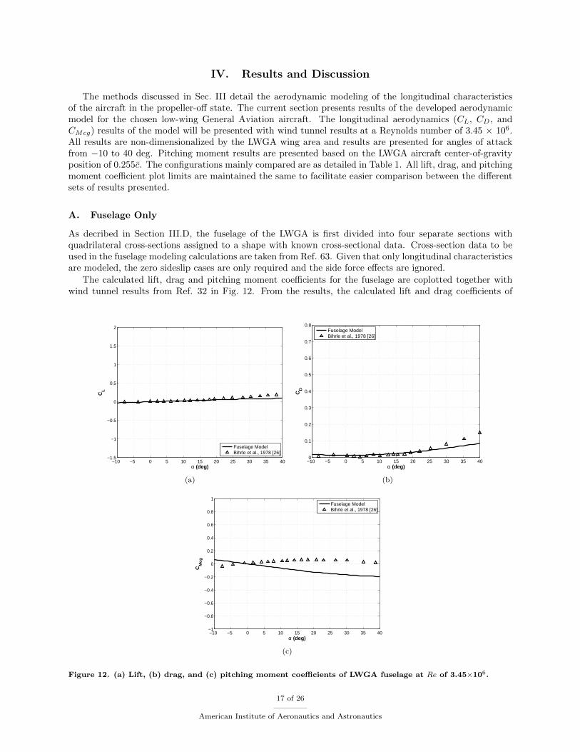
The next configuration analyzed is the fuselage-wing case. Experimental data for the NACA 642-415 airfoilwas used for the wing. Non-linear lifting line theory was used in calculating the lift and induced drag ofthe wing as detailed in Section III.C. The wing was divided into 30 spanwise panels. The converged liftcoefficient distribution along the LWGA wing at various angles of attack is shown in Fig. 13. The blackline represents the wing when viewed from behind. The effect of the fuselage is modeled as a region of zerolift at the center-span of the wing as shown in Fig. 13. The non-linear lifting line process is iterated untilconvergence. The red lines indicate the location of the aileron which for this case is not deflected.

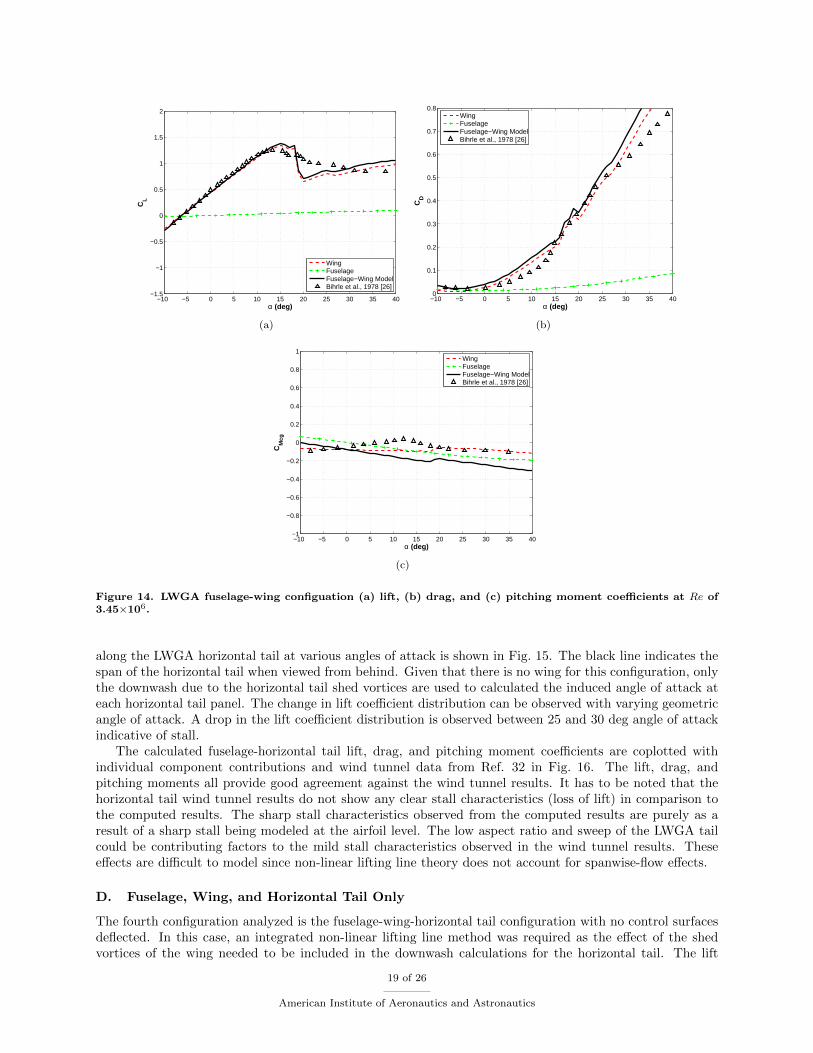
The calculated fuselage-wing configuration lift, drag, and pitching moment coefficients are coplotted withwind tunnel data from Ref. 32 in Fig. 14. In addition, individual component results are coplotted to showtheir contributions to the computed coefficients. The lift and drag coefficients give good agreement withthe wind tunnel results. The computed lift coefficients (Fig. 14(a)) show an overprediction in maximumlift and also a larger drop in lift post-stall when compared to the wind tunnel results. One of the primaryreasons for the discrepancy is the unavailability of experimental results for the modified NACA 642-415airfoil. Therefore, empirical methods had to be relied upon in modeling the stall and post-stall aerodynamiccharacteristics of the airfoil. The computed drag coefficients [Fig. 14(b)] matched the wind tunnel resultsin terms of its minimum drag. The wind tunnel results however show a wider drag bucket and a lessprecipitious drag rise at high angles of attack compared to the computed drag coefficients. As discussed inthe prior section, the pitching moment coefficient [Fig. 14(c)] results differ mainly due to the effect of thefuselage. Given that the center of gravity is located slightly aft of the quarter chord of the wing and that theairfoil has a relatively constant negative pitching moment pre-stall [see Fig. 3(c)] the wing pitching momentcontribution (red dashed line) is small to the overall aircraft.

C. Fuselage and Horizontal Tail Only

Similar to the previous section, for the fuselage-horizontal tail configuration, the horizontal tail was dividedinto 30 spanwise panels and the forces were computed using non-linear lifting line theory. The lift distribution

−4 −3 −2 −1 0 1 2 3 4−0.5

0

0.5

1

1.5

2

Cl

Distance (ft)

α = −10 degα = −5 degα = 0 degα = 5 degα = 10 degα = 15 degα = 20 degα = 25 deg

Figure 13. Lift distribution of LWGA wing in the fuselage-wing configuration at a Reynolds number of 3.45×106

at 5 deg angle of attack increments.

18 of 26


−10 −5 0 5 10 15 20 25 30 35 40−1.5

−1

−0.5

0

0.5

1

1.5

2

α (deg)

CL

WingFuselageFuselage−Wing ModelBihrle et al., 1978 [26]

(a)

−10 −5 0 5 10 15 20 25 30 35 400

0.1

0.2

0.3

0.4

0.5

0.6

0.7

0.8

α (deg)

CD


(b)

−10 −5 0 5 10 15 20 25 30 35 40−1

−0.8

−0.6

−0.4

−0.2

0

0.2

0.4

0.6

0.8

1

α (deg)

CM

cg


(c)

Figure 14. LWGA fuselage-wing configuation (a) lift, (b) drag, and (c) pitching moment coefficients at Re of3.45×106.

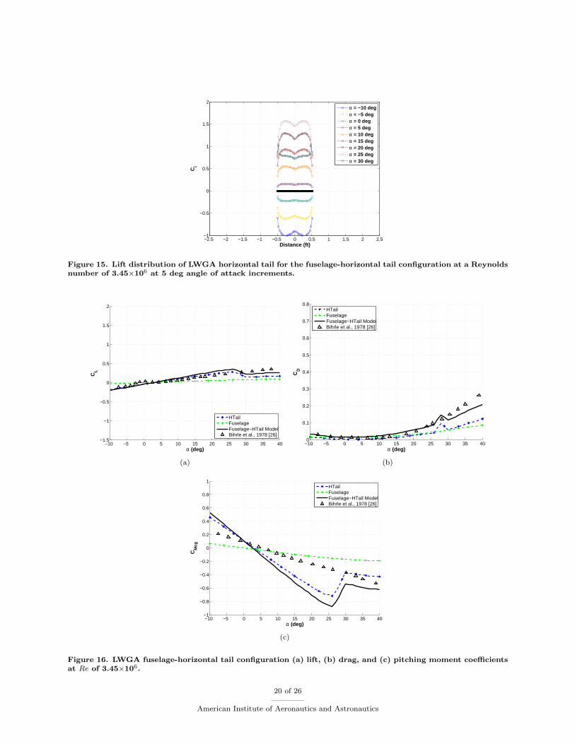
along the LWGA horizontal tail at various angles of attack is shown in Fig. 15. The black line indicates thespan of the horizontal tail when viewed from behind. Given that there is no wing for this configuration, onlythe downwash due to the horizontal tail shed vortices are used to calculated the induced angle of attack ateach horizontal tail panel. The change in lift coefficient distribution can be observed with varying geometricangle of attack. A drop in the lift coefficient distribution is observed between 25 and 30 deg angle of attackindicative of stall.

The calculated fuselage-horizontal tail lift, drag, and pitching moment coefficients are coplotted withindividual component contributions and wind tunnel data from Ref. 32 in Fig. 16. The lift, drag, andpitching moments all provide good agreement against the wind tunnel results. It has to be noted that thehorizontal tail wind tunnel results do not show any clear stall characteristics (loss of lift) in comparison tothe computed results. The sharp stall characteristics observed from the computed results are purely as aresult of a sharp stall being modeled at the airfoil level. The low aspect ratio and sweep of the LWGA tailcould be contributing factors to the mild stall characteristics observed in the wind tunnel results. Theseeffects are difficult to model since non-linear lifting line theory does not account for spanwise-flow effects.

D. Fuselage, Wing, and Horizontal Tail Only

The fourth configuration analyzed is the fuselage-wing-horizontal tail configuration with no control surfacesdeflected. In this case, an integrated non-linear lifting line method was required as the effect of the shedvortices of the wing needed to be included in the downwash calculations for the horizontal tail. The lift

19 of 26


−2.5 −2 −1.5 −1 −0.5 0 0.5 1 1.5 2 2.5−1

−0.5

0

0.5

1

1.5

2

Cl

Distance (ft)

α = −10 degα = −5 degα = 0 degα = 5 degα = 10 degα = 15 degα = 20 degα = 25 degα = 30 deg

Figure 15. Lift distribution of LWGA horizontal tail for the fuselage-horizontal tail configuration at a Reynoldsnumber of 3.45×106 at 5 deg angle of attack increments.

−10 −5 0 5 10 15 20 25 30 35 40−1.5

−1

−0.5

0

0.5

1

1.5

2

α (deg)

CL

HTailFuselageFuselage−HTail ModelBihrle et al., 1978 [26]

(a)

−10 −5 0 5 10 15 20 25 30 35 400

0.1

0.2

0.3

0.4

0.5

0.6

0.7

0.8

α (deg)

CD


(b)

−10 −5 0 5 10 15 20 25 30 35 40−1

−0.8

−0.6

−0.4

−0.2

0

0.2

0.4

0.6

0.8

1

α (deg)

CM

cg


(c)

Figure 16. LWGA fuselage-horizontal tail configuration (a) lift, (b) drag, and (c) pitching moment coefficientsat Re of 3.45×106.

20 of 26


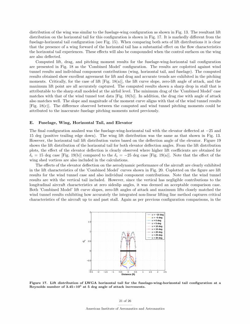
distribution of the wing was similar to the fuselage-wing configuration as shown in Fig. 13. The resultant liftdistribution on the horizontal tail for this configuration is shown in Fig. 17. It is markedly different from thefuselage-horizontal tail configuration (see Fig. 15). When comparing both sets of lift distributions it is clearthat the presence of a wing forward of the horizontal tail has a substantial effect on the flow characteristicsthe horizontal tail experiences. These effects will also be compounded when the control surfaces on the wingare also deflected.

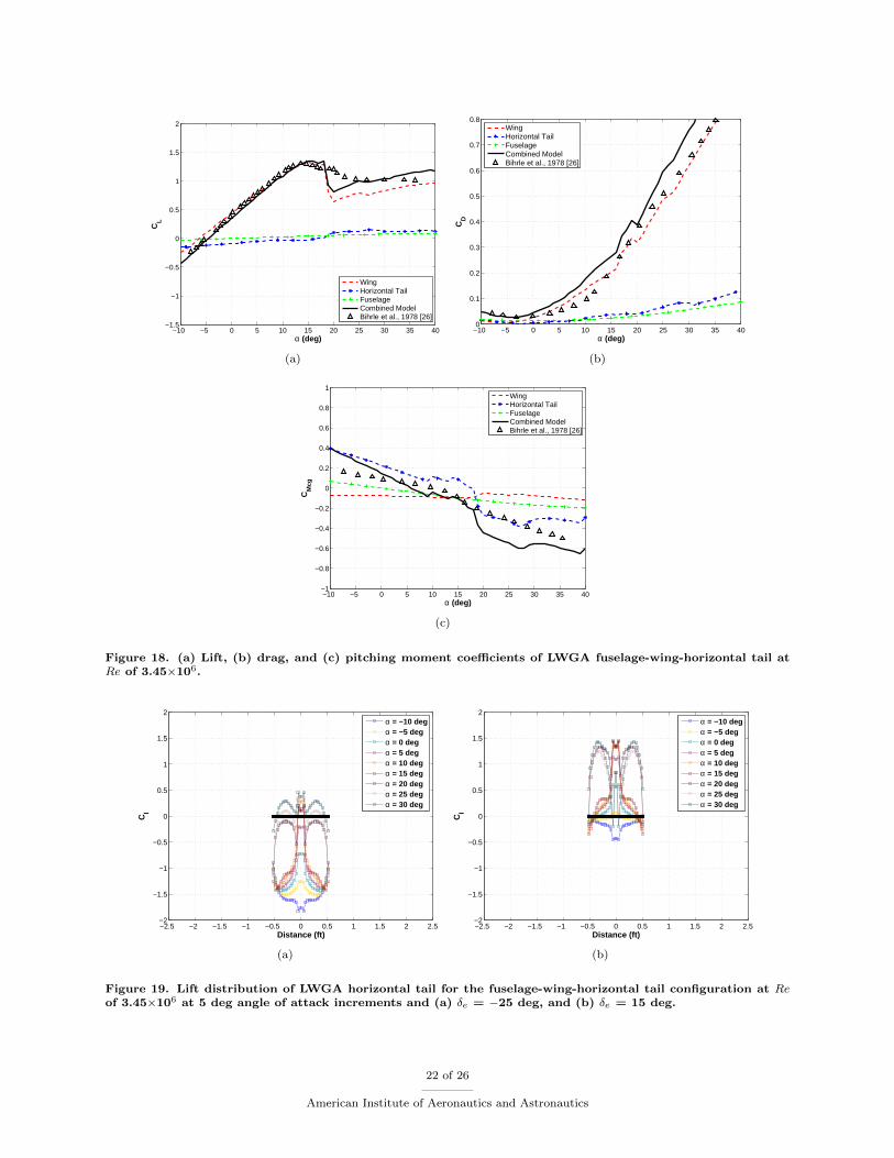
Computed lift, drag, and pitching moment results for the fuselage-wing-horizontal tail configurationare presented in Fig. 18 as the ’Combined Model’ configuration. The results are coplotted against windtunnel results and individual component contributions (wing, horizontal tail, and fuselage). The computedresults obtained show excellent agreement for lift and drag and accurate trends are exhibited in the pitchingmoments. Critically, for the case of lift [Fig. 18(a)], the lift curve slope, zero-lift angle of attack, and themaximum lift point are all accurately captured. The computed results shown a sharp drop in stall that isattributable to the sharp stall modeled at the airfoil level. The minimum drag of the ’Combined Model’ casematches with that of the wind tunnel test data [Fig. 18(b)]. In addition, the drag rise with angle of attackalso matches well. The slope and magnitude of the moment curve aligns with that of the wind tunnel results[Fig. 18(c)]. The difference observed between the computed and wind tunnel pitching moments could beattributed to the inaccurate fuselage pitching moments noted previously.

E. Fuselage, Wing, Horizontal Tail, and Elevator

The final configuration analzed was the fuselage-wing-horizontal tail with the elevator deflected at −25 and15 deg (positive trailing edge down). The wing lift distribution was the same as that shown in Fig. 13.However, the horizontal tail lift distribution varies based on the deflection angle of the elevator. Figure 19shows the lift distribution of the horizontal tail for both elevator deflection angles. From the lift distributionplots, the effect of the elevator deflection is clearly observed where higher lift coefficients are obtained forδe = 15 deg case [Fig. 19(b)] compared to the δe = −25 deg case [Fig. 19(a)]. Note that the effect of thewing shed vortices are also included in the calculations.

The effects of the elevator deflection on the aerodynamic performance of the aircraft are clearly exhibitedin the lift characteristics of the ’Combined Model’ curves shown in Fig. 20. Coplotted on the figure are liftresults for the wind tunnel case and also individual component contributions. Note that the wind tunnelresults are with the vertical tail included. However, since the vertical has negligible contributions to thelongitudinal aircraft characteristics at zero sideslip angles, it was deemed an acceptable comparison case.Both ’Combined Model’ lift curve slopes, zero-lift angles of attack and maximum lifts closely matched thewind tunnel results exhibiting how accurately the integrated non-linear lifting line method captures criticalcharacteristics of the aircraft up to and past stall. Again as per previous configuration comparisons, in the

−2.5 −2 −1.5 −1 −0.5 0 0.5 1 1.5 2 2.5−1

−0.5

0

0.5

1

1.5

2

Cl

Distance (ft)


Figure 17. Lift distribution of LWGA horizontal tail for the fuselage-wing-horizontal tail configuration at aReynolds number of 3.45×106 at 5 deg angle of attack increments.

21 of 26


−10 −5 0 5 10 15 20 25 30 35 40−1.5

−1

−0.5

0

0.5

1

1.5

2

α (deg)

CL

WingHorizontal TailFuselageCombined ModelBihrle et al., 1978 [26]

(a)

−10 −5 0 5 10 15 20 25 30 35 400

0.1

0.2

0.3

0.4

0.5

0.6

0.7

0.8

α (deg)

CD


(b)

−10 −5 0 5 10 15 20 25 30 35 40−1

−0.8

−0.6

−0.4

−0.2

0

0.2

0.4

0.6

0.8

1

α (deg)

CM

cg


(c)

Figure 18. (a) Lift, (b) drag, and (c) pitching moment coefficients of LWGA fuselage-wing-horizontal tail atRe of 3.45×106.

−2.5 −2 −1.5 −1 −0.5 0 0.5 1 1.5 2 2.5−2

−1.5

−1

−0.5

0

0.5

1

1.5

2

Cl

Distance (ft)


(a)

−2.5 −2 −1.5 −1 −0.5 0 0.5 1 1.5 2 2.5−2

−1.5

−1

−0.5

0

0.5

1

1.5

2

Cl

Distance (ft)


(b)

Figure 19. Lift distribution of LWGA horizontal tail for the fuselage-wing-horizontal tail configuration at Reof 3.45×106 at 5 deg angle of attack increments and (a) δe = −25 deg, and (b) δe = 15 deg.

22 of 26


−10 −5 0 5 10 15 20 25 30 35 40−1.5

−1

−0.5

0

0.5

1

1.5

2

α (deg)

CL


(a)

−10 −5 0 5 10 15 20 25 30 35 40−1.5

−1

−0.5

0

0.5

1

1.5

2

α (deg)

CL


(b)

Figure 20. Lift of LWGA fuselage-wing-horizontal tail at Re of 3.45×106 and δe of (a) −25 deg, (b) 15 deg.

−10 −5 0 5 10 15 20 25 30 35 400

0.1

0.2

0.3

0.4

0.5

0.6

0.7

0.8

α (deg)

CD


(a)

−10 −5 0 5 10 15 20 25 30 35 400

0.1

0.2

0.3

0.4

0.5

0.6

0.7

0.8

α (deg)

CD


(b)

Figure 21. Drag of LWGA fuselage-wing-horizontal tail at Re of 3.45×106 at δe of (a) −25 deg, (b) 15 deg.

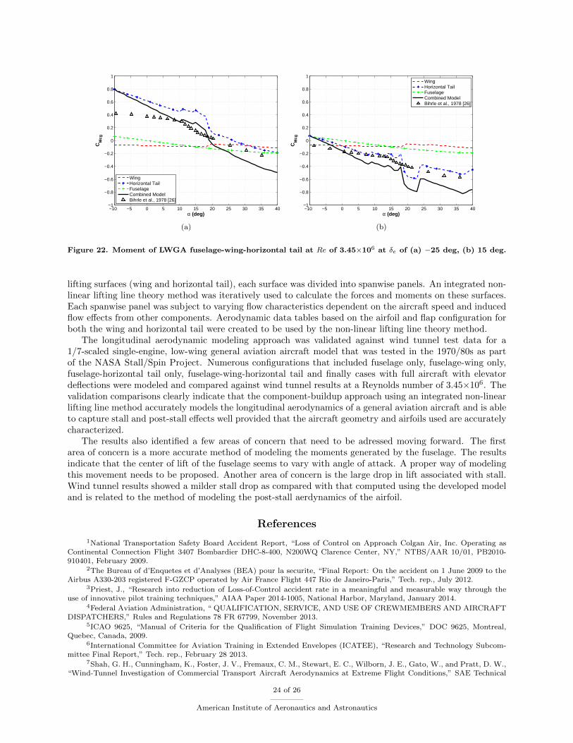
post-stall region, a sharper lift drop is computed as compared with the wind tunnel results.The drag (Fig. 21) and the moment (Fig. 22) results both follow general trends. The wing drag, however,

shows an overprediction in its results which results in an overprediction of the full aircraft drag comparedto the wind tunnel data. For the moment, similar order magnitude moments are observed when comparedto wind tunnel results. The effects of elevator deflection are clearly observed and is mainly due to the largemoment contributions from the horizontal tail.

V. Conclusions

This paper describes an approach taken to develop a high-fidelity longitudinal aerodynamic model forflight simulation of general aviation aircraft in the stall/post-stall regime. The aerodynamic model used isbased on the component-buildup method using strip theory. The aircraft is divided into individual compo-nents where for the current study, the fuselage, wing, and horizontal tail are separately modeled. A validatedengineering-type procedure was used to model the forces and moments of the fuselage. For the case of the

23 of 26


−10 −5 0 5 10 15 20 25 30 35 40−1

−0.8

−0.6

−0.4

−0.2

0

0.2

0.4

0.6

0.8

1

α (deg)

CM

cg


(a)

−10 −5 0 5 10 15 20 25 30 35 40−1

−0.8

−0.6

−0.4

−0.2

0

0.2

0.4

0.6

0.8

1

α (deg)

CM

cg


(b)

Figure 22. Moment of LWGA fuselage-wing-horizontal tail at Re of 3.45×106 at δe of (a) −25 deg, (b) 15 deg.

lifting surfaces (wing and horizontal tail), each surface was divided into spanwise panels. An integrated non-linear lifting line theory method was iteratively used to calculate the forces and moments on these surfaces.Each spanwise panel was subject to varying flow characteristics dependent on the aircraft speed and inducedflow effects from other components. Aerodynamic data tables based on the airfoil and flap configuration forboth the wing and horizontal tail were created to be used by the non-linear lifting line theory method.

The longitudinal aerodynamic modeling approach was validated against wind tunnel test data for a1/7-scaled single-engine, low-wing general aviation aircraft model that was tested in the 1970/80s as partof the NASA Stall/Spin Project. Numerous configurations that included fuselage only, fuselage-wing only,fuselage-horizontal tail only, fuselage-wing-horizontal tail and finally cases with full aircraft with elevatordeflections were modeled and compared against wind tunnel results at a Reynolds number of 3.45×106. Thevalidation comparisons clearly indicate that the component-buildup approach using an integrated non-linearlifting line method accurately models the longitudinal aerodynamics of a general aviation aircraft and is ableto capture stall and post-stall effects well provided that the aircraft geometry and airfoils used are accuratelycharacterized.

The results also identified a few areas of concern that need to be adressed moving forward. The firstarea of concern is a more accurate method of modeling the moments generated by the fuselage. The resultsindicate that the center of lift of the fuselage seems to vary with angle of attack. A proper way of modelingthis movement needs to be proposed. Another area of concern is the large drop in lift associated with stall.Wind tunnel results showed a milder stall drop as compared with that computed using the developed modeland is related to the method of modeling the post-stall aerdynamics of the airfoil.

References

1National Transportation Safety Board Accident Report, “Loss of Control on Approach Colgan Air, Inc. Operating asContinental Connection Flight 3407 Bombardier DHC-8-400, N200WQ Clarence Center, NY,” NTBS/AAR 10/01, PB2010-910401, February 2009.

2The Bureau of d’Enquetes et d’Analyses (BEA) pour la securite, “Final Report: On the accident on 1 June 2009 to theAirbus A330-203 registered F-GZCP operated by Air France Flight 447 Rio de Janeiro-Paris,” Tech. rep., July 2012.

3Priest, J., “Research into reduction of Loss-of-Control accident rate in a meaningful and measurable way through theuse of innovative pilot training techniques,” AIAA Paper 2014-1005, National Harbor, Maryland, January 2014.

4Federal Aviation Administration, “ QUALIFICATION, SERVICE, AND USE OF CREWMEMBERS AND AIRCRAFTDISPATCHERS,” Rules and Regulations 78 FR 67799, November 2013.

5ICAO 9625, “Manual of Criteria for the Qualification of Flight Simulation Training Devices,” DOC 9625, Montreal,Quebec, Canada, 2009.

6International Committee for Aviation Training in Extended Envelopes (ICATEE), “Research and Technology Subcom-mittee Final Report,” Tech. rep., February 28 2013.

7Shah, G. H., Cunningham, K., Foster, J. V., Fremaux, C. M., Stewart, E. C., Wilborn, J. E., Gato, W., and Pratt, D. W.,“Wind-Tunnel Investigation of Commercial Transport Aircraft Aerodynamics at Extreme Flight Conditions,” SAE Technical

24 of 26


Paper 2002-01-2912, Phoenix, Arizona, November 2002.8Cunningham, K., Foster, J. V., Shah, G. H., and Stewart, E. C., “Simulation Study of a Commercial Transport Airplane

During Stall and Post-Stall Flight,” SAE Technical Paper 2004-01-3100, Reno, Nevada, November 2004.9Foster, J. V., Cunningham, K., Fremaux, C. M., Shah, G. H., Stewart, E. C., Rivers, R. A., Wilborn, J. E., and Gato, W.,

“Dynamics Modeling and Simulation of Large Transport Airplanes in Upset Condition,” AIAA Paper 2005-5933, San Francisco,California, August 2005.

10M. M. Murch and J. V. Foster, “Recent NASA Research on Aerodynamic Modeling of Post-Stall and Spin Dynamics ofLarge Transport Airplanes,” AIAA Paper 2007-463, Reno, NV, Jan. 2007.

11Murch, A. M., Aerodynamic Modeling of Post-Stall and Spin Dynamics of Large Transport Airplanes, Master’s thesis,School of Aerospace Engineering, Georgia Institute of Technology, Atlanta, Georgia, August 2007.

12Fucke, L., Biryukov, V., Grigorev, M., Rogozin, V., Groen, E., Wentink, M., Field, J., Soemarwoto, B., Abramov, N.,Goman, M., and Khrabrov, A., “Developing Scenarios for Research into Upset Recovery Simulation,” AIAA Paper 2010-7794,Toronto, Ontario, August 2010.

13Abramov, N., Goman, M., Khrabrov, A., Kolesnikov, E., Sidoruk, M., Soemarwoto, B., and Smaili, H., “AerodynamicModel of Transport Airplane In Extended Envelope for Simulation of Upset Recovery,” Paper ICAS 2012-3.1.2, Brisbane,Australia, September 2012.

14Groen, E., Ledegang, W., Field, J., Smaili, H., Roza, M., Fucke, L., Nooij, S., Goman, M., Mayrhofer, M., Zaichik,L., Grigoryev, M., and Biyukov, V., “SUPRA Enhanced Upset Recovery Simulation,” AIAA Paper 2012-4630, Minneapolis,Minnesota, August 2012.

15Abramov, N. B., Goman, M. G., Khrabrov, A. N., Kolesnikov, E. N., Fucke, L., Soemarwoto, B., and Smaili, H., “PushingAhead - SUPRA Airplane Model for Upset Recovery,” AIAA Paper 2012-4631, Minneapolis, Minnesota, August 2012.

16Khrabov, A., Sidoryuk, M., and Goman, M., “Aerodynamic Model Development and Simulation of Airliner Spin forUpset Recovery,” Progress in Flight Physics, Vol. 5, 2013, pp. 621–636.

17Air Safety Institute, “General Aviation Accidents in 2010,” 22nd Joseph T. Nall Report, 2013.18National Transportation Safety Board, “Review of U.S. Civil Aviation Accidents: Review of Aircraft Accident Data

2010,” NTSB ARA-12/01, Washington D.C, 2010.19National Transportation Safety Board, “NTSB 2015 Most Wanted Transportation Safety Improvements: Prevent Loss

of Control In Flight in General Aviation,” NTSB Brochure, Washington D.C, 2015.20National Transportation Safety Board, “NTSB 2015 Most Wanted Transportation Safety Improvements: Prevent Loss

of Control In Flight in General Aviation,” NTSB Brochure, Washington D.C, 2016.21Anonymous, “Partnership to Enhance General Aviation Safety, Accessibility and Sustainability,” https://www.pegasas.

aero/, Accessed Apr. 2016.22Microsoft, “Flight Simulator X,” http://www.fsxworld.com/products/, Accessed Sep. 2015.23GNU General Public Open Source License, “FlightGear Flight Simulator,” http://www.flightgear.org/, Accessed Sep.

2015.24Lockheed Martin, “Prepare3D,” http://www.prepar3d.com/, Accessed Sep. 2015.25Pizkin, S. T. and Levinsky, E. S., “Nonlinear Lifting Line Theory for Predicting Stalling Instabilities on Wings of

Moderate Aspect Ratio,” Report No. CASD-NCS-76-001, June 1976.26Lutze, F. H. and Lluch, D., “Simulation of stall, spin, and recovery of a general aviation aircraft,” AIAA Paper 1996-3409,

San Diego, CA, July 1996.27Keller, J. D., McKillip, R. M., Jr., and Wachpress, D. A., “Physical Modeling of Aircraft Upsets for Real-Time Simulation

Applications,” AIAA Paper 2008-6205, Honolulu, Hawaii, August 2008.28Selig, M. S., “Real-Time Flight Simulation of Highly Maneuverable Unmanned Aerial Vehicles,” Journal of Aircraft ,

Vol. 51, No. 6, 2014, pp. 1705–1725.29Selig, M. S., “Modeling Propeller Aerodynamics and Slipstream Effects on Small UAVs in Realtime,” AIAA Paper Invited

Paper, to be published 8/2/2010, 2010.30Laminar Research, “X-Plane,” http://www.x-plane.com/desktop/home/, Accessed Sep. 2015.31Paul, R. and Gopalarathnam, A., “Simulation of Flight Dynamics with an Improved Post-Stall Aerodynamics Model,”

AIAA Paper 2012-4956, August 2012.32Bihrle, W., Jr., Barnhart, B., and Pantason, P., “Static Aerodynamic Characteristics of a Typical Single Engine Low-

Wing General Aviation Design for an Angle-of-Attack Range of -8 deg to 90 deg,” NASA CR-2971, July 1978.33Bowman, J. S. and Burk, S. M., Jr., “Stall/Spin Research Status Report,” Business Aircraft Meeting Report 740354,

Wichita, KS, April 1974.34Gloudemans, J. R., Davis, P. C., and Gelhausen, P. A., “A Rapid Geometry Modeler for Conceptual Aircraft,” AIAA

Paper 96-0052, Reno, NV, Jan. 1996.35Gloudemans, J. R., McDonald, R., Moore, M., Hahn, A., Fredericks, B., and Gary, A., “Open Vehicle Sketch Pad,”

http://openvsp.org/, Accessed Jan. 2015.36Riley, D. R., “Simulator Study of the Stall Departure Characteristics of a Light General Aviation Airplane with or

without a Wing-Leading-Edge Modification,” NASA TM-86309, May 1985.37Funk Jr., J. D. and McCormick, B. W., “Simulation of Stall Departure using a Nonlinear lifting-line Model,” AIAA

Paper 91-0340, Reno, NV, Jan. 1991.38Anderson, J. D., Jr., Corda, S., and Van Wie, D. M., “Numerical lifting-line Theory Applied to Drooped Leading-Edge

Wings below and above Stall,” Journal of Aircraft , Vol. 17, No. 12, 1980, pp. 809–904.39Drela, M., “XFOIL: An Analysis and Design System for Low Reynolds Number Airfoils,” Low Reynolds Number Aero-

dynamics, edited by T. J. Mueller, Vol. 54 of Lecture Notes in Engineering, Springer-Verlag, New York, June 1988, pp. 1–12.

25 of 26


https://www.pegasas.aero/

https://www.pegasas.aero/

http://www.fsxworld.com/products/

http://www.flightgear.org/

http://www.prepar3d.com/

http://www.x-plane.com/desktop/home/

http://openvsp.org/

40Selig, M. S., Donovan, J. F., and Fraser, D. B., Airfoils at Low Speeds, Soartech 8, SoarTech Publications, VirginiaBeach, Virginia, 1989.

41Selig, M. S., Guglielmo, J. J., Broeren, A. P., and Giguere, P., Summary of Low-Speed Airfoil Data, Vol. 1 , SoarTechPublications, Virginia Beach, Virginia, 1995.

42Selig, M. S., Lyon, C. A., Giguere, P., Ninham, C. N., and Guglielmo, J. J., Summary of Low-Speed Airfoil Data, Vol. 2 ,SoarTech Publications, Virginia Beach, Virginia, 1996.

43Lyon, C. A., Broeren, A. P., Giguere, P., Gopalarathnam, A., and Selig, M. S., Summary of Low-Speed Airfoil Data,Vol. 3 , SoarTech Publications, Virginia Beach, Virginia, 1998.

44Selig, M. S. and McGranahan, B. D., “Wind Tunnel Aerodynamic Tests of Six Airfoils for Use on Small Wind Turbines,”National Renewable Energy Laboratory, NREL/SR-500-35515, 2004.

45Selig, M. S., Deters, R. W., and Williamson, G. A., “Wind Tunnel Testing Airfoils at Low Reynolds Numbers,” AIAAPaper 2011-875, January 2011.

46Abbott, I. H. and von Doenhoff, A. E., Theory of Wing Sections, Including a Summary of Airfoil Data, Dover Bookson Aeronautical Engineering Series, Dover Publications, 1959.

47Sheldahl, R. E. and Klimas, P. C., “Aerodynamic Characteristics of Seven Airfoil Sections Through 180-Degree of Attackfor Use in Aerodynamic Analysis of Vertical Axis Wind Turbines,” Sandia National Laboratories, SAND80-2114, Albuquerque,NM, 1981.

48Ostowari, C. and Naik, D., “Post-Stall Wind Tunnel Data for NACA 44XX Series Airfoil Sections,” SERI/STR-217-2559,January 1985.

49Snyder, M. H., Wentz, W. H., and Anwar, A., “Two Dimensional Tests of Four Airfoils at Angles of Attack from 0 to360 degrees,” Wichita State University, Center for Energy Studies, 1981.

50Satran, D. and Snyder, M. H., “Two Dimensional Tests of GA(W)-1 and GA(W)-2 Airfoils at Angles-of-Attack from 0to 360 Degrees,” Wichita State University, Center for Energy Studies, 1977.

51Rumsey, C., “Overview and Summary of the Second AIAA High-Lift Prediction Workshop,” Journal of the Aircraft ,Vol. 52, No. 4, 2015, pp. 1006–1025.

52Coder, J. G. and Maughmer, M. D., “Comparisons of Theoretical Methods for Predicting Airfoil Aerodynamic Charac-teristics,” Journal of Aircraft , Vol. 51, No. 1, 2014, pp. 183–191.

53Spera, D. A., “Models of Lift and Drag Coefficients of Stalled and Unstalled Airfoils in Wind Turbines and WindTunnels,” NASA CR-2008-215434, October 2008.

54Lindenburg, C., “Stall Coefficients,” Energy Research Center of the Netherlands, Petten, ECN-RX-01-004, January 2001,Presented at IEA Symposium on the Aerodynamics of Wind Turbines, National Renewable Energy Laboratory, Golden, CO,December, 2000.

55Tangler, J. L. and Ostowari, C., “Horizontal Axis Wind Turbine Post Stall Airfoil Characteristics Synthesization,”Presented at the Horizontal-Axis Wind Turbine Technology Conference, Cleveland, OH, May, 1984.

56Montgomerie, B., “Methods for Root Effects, Tip Effects and Extending the Angle of Attack Range to ±180 deg, withApplication to Aerodynamics for Blades on Wind Turbines and Propellers,” FOI-R 1305-SE, Stockholm, Sweeden, June 2004.

57Torenbeek, E., Synthesis of Subsonic Airplane Design, Springer Science & Business Media, 1982.58McCormick, B. W., Aerodynamics, Aeronautics, and Flight Mechanics, John Wiley & Sons, New York, NY, 2nd ed.,

1995.59Owens, D. B., “Weissinger’s Model of the Nonlinear Lifting-Line Method for Aircraft Design,” AIAA Paper 98-0597,

Reno, NV, Jan. 1998.60Phillips, W. F. and Snyder, D. O., “Application of Lifting-Line Theory to Systems of Lifting Surfaces,” AIAA Paper

2000-0653, Reno, NV, Jan. 2000.61Bertin, J. J., Aerodynamics for Engineers, Fourth Edition, Pearson Education, 2006.62Kelley, H. R., “The Estimation of Normal-Force, Drag, and Pitching-Moment Coefficients for Blunt-Based Bodies of

Revolution at Large Angles of Attack,” Journal of the Aeronautical Sciences, Vol. 21, No. 8, 1954, pp. 549–555.63Polhamus, E., “A Review of Some Reynolds Number Effects Related to Bodies at High Angles of Attack,” NASA

CR-3809, August 1984.64Jorgensen, L. H. and Brownson, J. J., “Effects of Reynolds number and Body Corner Radius on Aerodynamic Charac-

teristics of a Space Shuttle-Type Vehicle at Subsonic Mach Numbers,” NASA TN D-6615, Jan. 1972.65Jorgensen, L. H., “A Method for Estimating Static Aerodynamic Characteristics for Slender Bodies of Circular and

Noncircular Cross Section Alone and With Lifting Surfaces at Angles of Attack from 0 deg to 90 deg,” NASA TN D-7228, April1973.

66Allen, H. J. and Perkins, E. W., “A Study of Effects of Viscosity on Flow over Slender Inclined Bodies of Revolution,”NACA TR-1048, Jan. 1951.

67Polhamus, E., “Effect of Flow Incidence and Reynolds Number on Low-Speed Aerodynamic Characteristics of SeveralNoncircular Cylinders with Applications to Directional Stability and Spinning,” NASA TN-4176, Jan. 1958.

26 of 26


Stall/Post-Stall Modeling of the Longitudinal Characteristics of a...

Documents

Transcript of Stall/Post-Stall Modeling of the Longitudinal Characteristics of a...