Stainless Steel Bonded to Concrete: An Experimental ... · Abstract: The durability performance of...

Stainless Steel Bonded to Concrete: An Experimental Assessmentusing the DIC Technique

Hugo Biscaia1),* , Noel Franco2) , and Carlos Chastre3)

(Received June 17, 2017, Accepted October 24, 2017)

Abstract: The durability performance of stainless steel makes it an interesting alternative for the structural strengthening of

reinforced concrete. Like external steel plates or fibre reinforced polymers, stainless steel can be applied using externally bonded

reinforcement (EBR) or the near surface mounted (NSM) bonding techniques. In the present work, a set of single-lap shear tests

were carried out using the EBR and NSM bonding techniques. The evaluation of the performance of the bonding interfaces was

done with the help of the digital image correlation (DIC) technique. The tests showed that the measurements gathered with DIC

should be used with caution, since there is noise in the distribution of the slips and only the slips greater than one-tenth of a

millimetre were fairly well predicted. For this reason, the slips had to be smoothed out to make it easier to determine the strains in

the stainless steel and the bond stress transfer between materials, which helps to determine the bond–slip relationship of the

interface. Moreover, the DIC technique allowed to identify all the states developed within the interface through the load–slip

responses which were also closely predicted with other monitoring devices. Considering the NSM and the EBR samples with the

same bonded lengths, it can be stated that the NSM system has the best performance due to their higher strength, being observed

the rupture of the stainless steel in the samples with bond lengths of 200 and 300 mm. Associated with this higher strength, the

NSM specimens had an effective bond length of 168 mm which is 71.5% of that obtained for the EBR specimens (235 mm). A

trapezoidal and a power functions are the proposed shapes to describe the interfacial bond–slip relationships of the NSM and EBR

systems, respectively, where the maximum bond stress in the former system is 1.8 times the maximum bond stress of the latter one.

Keywords: stainless steel, concrete, bond failure, digital image correlation.

1. Introduction

The first studies on the external bonded reinforcement(EBR) technique using steel plates were carried out in thelate 1960s in France by L’Hermite and Bresson, who ana-lyzed the steel-epoxy-concrete connection (L’Hermite andBresson 1967; L’Hermite 1977). Since then, there have beenmany studies characterizing the bonding behaviour ofstrengthening elements using the EBR technique, initially

with steel plates (Ladner 1978, 1983; Jones et al. 1980;Swamy and Jones 1980; Chastre Rodrigues 1993; Taljsten1997) and more recently with fibre reinforced polymers(FRP) (Blaschko and Zilch 1999; De Lorenzis et al. 2000;De Lorenzis and Teng 2007; Lorenzis et al. 2001; Nakabaet al. 2001; Chen et al. 2005; Aiello and Leone 2008;Martinelli et al. 2011; Dehghani et al. 2012; Biscaia et al.2013, 2014). As for the near surface mounted (NSM) tech-nique, although there are some references of its use, only atthe end of the 1990s did studies on the performance of thistechnique associated with the use of FRP rods (Blaschko andZilch 1999; De Lorenzis et al. 2000) begin to appear.Therefore, in most of the studies that can be found in the

literature (e.g. Xia 2005; Akbar et al. 2010; Smith 2010;Wan 2010; Wan et al. 2014; Biscaia et al. 2016a, b, 2017b),the focus is on bonded joints between FRP composites andconcrete but recently there have been more studies on bothsteel (only with EBR technique) and timber structures (withboth EBR and NSM techniques). Still, in reinforced concrete(RC) structural strengthening, stainless steel (SS) is a pos-sible alternative to mild steel or FRP composites due to itsdurability. Compared to mild steel, the durability perfor-mance of SS is higher, but there is no significant differencebetween them in terms of weight-strength ratio. However,despite its lower weight/strength ratio, stainless steel hasductile behaviour, and good corrosion resistance which are

1)Fluid and Structures Engineering, Research and

Development Unit in Mechanical and Industrial

Engineering, Department of Civil Engineering,

Faculdade de Ciencias e Tecnologia, Universidade Nova

de Lisboa, Caparica, Portugal.

*Corresponding Author; E-mail: [email protected])Department of Civil Engineering, Faculdade de

Ciencias e Tecnologia, Universidade Nova de Lisboa,

2829-516 Caparica, Portugal.3)Civil Engineering Research and Innovation for

Sustainability, Institute of Structural Engineering,

Territory and Construction, Department of Civil

Engineering, Faculdade de Ciencias e Tecnologia,

Universidade Nova de Lisboa, Caparica, Portugal.

Copyright � The Author(s) 2018. This article is an open

access publication

International Journal of Concrete Structures and MaterialsDOI 10.1186/s40069-018-0229-8ISSN 1976-0485 / eISSN 2234-1315

http://orcid.org/0000-0002-4791-5123

http://orcid.org/0000-0002-5169-0609

http://orcid.org/0000-0002-7708-6995

http://crossmark.crossref.org/dialog/?doi=10.1186/s40069-018-0229-8&domain=pdf

http://crossmark.crossref.org/dialog/?doi=10.1186/s40069-018-0229-8&domain=pdf

important and decisive factors in choosing it for strength-ening structures instead of FRP composites. Nevertheless, asignificant and common drawback, whatever the bondedmaterials are, is the premature debonding of the materialused in the bonding strengthening technique. Several authorshave been studying the premature debonding phenomenonon FRP composites and concrete joints (e.g. Arduini et al.1997; Neubauer and Rostasy 1997; Bizindavyi and Neale1999; Harmon et al. 2003; Smith and Teng 2002; Yao et al.2005; Teng et al. 2006; Wu and Yin 2003), FRP and timberjoints (e.g. Smith 2010; Wan 2010; Wan et al. 2014; Biscaiaet al. 2016a, b, 2017), FRP and steel joints (e.g. Xia andTeng 2005; Akbar et al. 2010; Fawzia et al. 2006; Wanget al. 2016; Yu et al. 2012; Al-Mosawe et al. 2015; Fernandoet al. 2014) or steel and concrete joints (e.g. L’Hermite andBresson 1967; L’Hermite 1977; Ladner 1978; Ladner 1983;Jones et al. 1980; Swamy and Jones 1980; Chastre Rodri-gues 1993; Taljsten 1997; Gomes and Appleton 1999; VanGermet 1990; Aykac et al. 2013).Therefore, researchers have studied the debonding phe-

nomenon between two bonded materials through differentapproaches whether they are experimental, analytical,numerical or embracing part or all of these three procedures.Furthermore, the test setup configuration assumed for thiskind of study may vary considerably (Wu et al. 2002), withthe most commonly used configurations being the double-lap pull or push shear tests, the single-lap pull tests, thedouble strap tests or the 3-point bending tests. Independentlyof the procedure followed, researchers seem to be fairlyunanimous that the debonding failure process of a struc-turally bonded joint can be analyzed and predicted throughthe relationship between the interfacial bond stress and theslip (i.e. the relative displacement between bondedmaterials).Unlike FRP composites, stainless steel has a more com-

plex constitutive behaviour, which may change or eveneliminate conventional ways of finding the bond–slip rela-tionship. Typically, the bond stresses and the slips areexperimentally found in the data collected from strain gau-ges that, before the testing of the samples, were bonded onthe strengthening material along their bond length. Thus, todetermine the bond stresses, it is assumed that the bondstresses developed between two consecutive strain gaugesare constant. To determine the slips, it is first assumed thatthe strains in the concrete are zero and, by integrating thestrains with respect to (and along) the bonded length, theslips within the interface can then be calculated. Dai et al.(2005) proposed an alternative procedure, which eliminatesthe need to use strain gauges. To determine the interfacialbond–slip relationship, they said that knowing only thedisplacement at the most loaded end of the strengtheningmaterial and the load transmitted to that material is enoughto obtain the bond–slip relationship. In both cases, a suffi-ciently long bond length should be considered, but the for-mer method makes the process more expensive because itrequires the use of several strain gauges that should not bebonded too far away from each other in order to obtainfeasible results.

A more recent alternative to obtain the slips developedwithin a bonded joint is digital image correlation (DIC),which allows the monitoring of an entire surface (Almeidaet al. 2016) instead of a single point, as conventional straingauges do. Once again, researchers have been studying thebond between an FRP composite and concrete (e.g. Marti-nelli et al. 2011; Czaderski et al. 2010; Cruzet al. 2016;Ghiassi et al. 2013; Zhu et al. 2014). The use of commercialDIC techniques is quite expensive but, nowadays, its usebecame very economical due to the powerful digital camerascurrently available on the market, plus the free software thatcan be easily found on the web (e.g. Wang and Vo 2012;http://www.ncorr.com/; GOM Correlate) to perform the DICanalysis. However, the reliability of these free software forthe assessment of the debonding phenomenon betweenstainless steel and concrete was not demonstrated so far butits use is unlimited and besides that, to start monitoringlaboratory structures under loading, only the initial cost ofthe digital camera and the corresponding free softwareinstalled in a laptop, is needed.Although some work suggests that the DIC technique can

be used to determine the interfacial bond–slip relationship ofCFRP-to-concrete interfaces (Ghiassi et al. 2013; Zhu et al.2014), the bond stresses are generally smoothed through amathematical function that predicts the slips or the straindistributions in the FRP composite. This procedure bypassesthe difficulties with obtaining a smoothed displacement resultfrom the DIC technique and the slips fluctuate instead (Zhuet al. 2014). Therefore, when it comes to determining thestrains and especially the bond stresses in the interface, thefluctuations in the slip distributions are amplified, whichincreases the error in calculating the interfacial bond–sliprelationship. For this reason, a smoothed and previouslyknown function of the slips or strain distributions is usedinstead of the real ‘‘peaks and valleys’’ obtained from the DICtechnique. However, it is important to note that determiningthe interfacial bond–slip relationships with DIC can only beviable if the results gathered by using the DIC technique canreproduce the same bond–slip relationship accurately enoughand on its own, as the results obtained from other means, suchas those reached by the two procedures mentioned earlier.Knowing the interfacial bond–slip relationship within thestainless steel and the concrete due to their bonding with anadhesive is important because it will open up the possibilityto analyze and study, using an analytical or a numericalapproach, the debonding failure between the stainless steeland concrete by means of either a closed-form solution or byan approximation procedure, respectively.However, to the best knowledge of the authors, there are

no studies covering the bond behaviour of the stainless steelbonded to concrete and therefore, the present work aims topresent an experimental study in which the bonded interfacebetween the stainless steel and the concrete is tested withdifferent bond lengths. Furthermore, stainless steel strips androds were used. The stainless steel strips were bonded on thesurface of several RC samples using the Externally BondedReinforcement (EBR) bonding technique, whilst the rodswere bonded into a groove previously made on the surface of

International Journal of Concrete Structures and Materials

http://www.ncorr.com/

the RC samples as per the Near Surface Technique (NSM).To monitor the strains in the EBR specimens, several straingauges were used. In order not to affect the bonded area ofthe NSM specimens, no strain gauges were used in thesesamples. In both cases, the DIC technique was used and itsviability was checked with the EBR specimens only. In somecases, only the most loaded bonded region could be moni-tored with the DIC technique due to the range of the bondedlengths covered in this work (between 50 and 800 mm).Still, throughout the duration of the tests the slips were quiteaccurate compared with those obtained from the straingauges and the load–slip response at the stainless steel loa-ded end was sufficiently reproduced using the DIC tech-nique. Moreover, the slip distributions observed with theDIC technique showed similarities to those obtained fromthe strain gauges, despite some fluctuations, i.e. with higherslips at the SS loaded end and decreasing towards the SS freeend. However, as initially suspected, the differences betweenthe strains from the DIC technique and the strain gaugesincreased throughout. The interfacial bond–slip relationshipbetween the stainless steel and concrete of the EBR speci-men was then determined from the strain gauges bonded onthe stainless steel strips. The results obtained from the EBRspecimens, allowed a first attempt to be shown to representand qualitatively identify the bond–slip relationship of theNSM specimens. Nevertheless, it was also found that theNSM specimens and the stainless steel rods performed betterdue to the rupture of the stainless steel rods when the bondedlength was equal to or higher than 200 mm long.

2. Experimental Program

In order to evaluate the Mode II bond transfer betweenstainless steel (SS) and concrete, an experimental programincluding two different bonding techniques was idealized.The Externally Bonding Reinforcement (EBR) and the nearsurface mounted (NSM) techniques were herein considered.Several bond lengths were tested and their influence on thestrength of the interface was analyzed. Table 1 shows all thetests carried out as well as the designation of the specimensgiven to each one. Additionally, the instrumentation used oneach test is also briefly mentioned in Table 1.

2.1 Mechanical Properties of the MaterialsThe specimens used for the present experimental program

were taken from RC T-beams previously tested to a 4-pointbending test (Franco and Chastre 2016; Chastre et al.2016, 2017). The regions of the beams with negligiblebending moments, i.e. at the vicinities of the supports (pin-rolled), were used and the stainless steel was bonded at thebottom region of the flange of the T-beam with their endsfree of any additional mechanical anchorages. This proce-dure ensures that the concrete used was not sufficientlytensioned to develop or even initiate any cracks that couldaffect the results obtained now from the single-lap sheartests. The strength of the concrete was evaluated at 28 daysof age and 3 concrete cubes were subjected to uniaxial

compression until failure accordingly to the standard NP EN12390-3 (CEN 2003). The results allowed the averagemaximum compression stress of the concrete to be calcu-lated by fcm = 24.1 MPa, which represents, accordingly toEurocode 2 (Eurocode 2 (EC2) 1992), a C20/25 concrete.The steel reinforcements of the RC T-beams were also

tested under uniaxial tension and its mechanical propertiesare briefly reported in Table 2. More details about the testsof the steel reinforcements can be found elsewhere (Francoand Chastre 2016; Chastre et al. 2017; Chastreet al. 2016).The mechanical properties of the stainless steel were alsodetermined from the tensile tests carried out on 7 strips witha cross section of 20 9 5 mm (width 9 thickness) and from6 tests on rods with 8 mm diameter, according to theEuropean standard EN ISO 6892-1 (CEN 2009). The resultsobtained from these tests are shown in Table 2.For the bonding of the stainless steel to the concrete, an

epoxy resin was used with the commercial designation S&PResin 220. The mechanical properties of the epoxy resingiven by the supplier were herein considered (S&P Resin220 2016), i.e. compression strength higher than 70 MPa,shear strength higher than 26 MPa, Young modulus higherthan 7.1 GPa, bond stress when used with concrete and at20 �C higher than 3 MPa and bond stress to steel at 20 �Chigher than 14 MPa (after 3 days).The yielding point of the stainless steel strips is not clearly

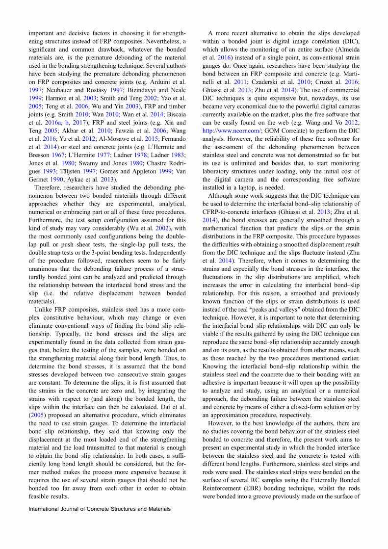
identified due to its constitutive nonlinearities, existing at alow strain level, whereas the constitutive behaviour of thestainless steel rods is elastic–plastic with a yielding pointvery clear and easy to identify. Therefore, the constitutivebehaviour of the stainless steel strips was approximated tothe Ramberg–Osgood relationship (Ramberg 1943) inaccordance to:

ess ¼rssEss

þ a � rssEss

� rssr0

� �n�1

ð1Þ

where a and n are constants obtained from experimentaltensile test of the stainless steel strip and r0 is the axial stressin the stainless steel at 0.2% strain. Hence, in the presentstudy, the values determined for a and n are 0.05 and 9.7,respectively. Figure 1 shows the stress–strain relationshipsof the stainless steel in strips and rods obtained from thesimple tensile tests carried out in a universal tensile machinewith a capacity of 100 kN.

2.2 Geometry and Preparationof the SpecimensAs mentioned earlier, for the single-lap shear tests, the

specimens were based on short lengths of RC T-beams andstainless steel bonded on uncracked concrete regions. Thecross section and the corresponding geometry of theT-beams are shown in Fig. 2a, whereas Fig. 2b shows thecross section of the specimen in which the EBR techniquewas used. It should be noted that all of the specimens had thesame concrete covering of 20 mm and the stirrups werespaced between them at every 150 mm. The reinforcedconcrete had a total height of 305 mm, in which 105 mm


form to the flange. The flange was 405 mm wide and theweb measured 150 mm wide. The stainless steel was alwaysbonded along the mid line that equally divides the flange inhalf. For the EBR system, the concrete surface was pre-treated with grinder, whereas for the NSM system, a smallgroove with 12 mm deep was made in the concrete surfacein order to insert the stainless steel rod. The stainless steelstrips and rods were all pre-treated with wire brush and thencleaned with compressed air and acetone before starting tobond the SS to the concrete in order to remove contaminantson the surface of the stainless steel (e.g. oil, grease, water,etc.) (Fernando et al. 2013).The EBR system was completed when the epoxy resin was

placed on the concrete surface along the bond length and thestainless steel positioned on the resin. For the NSM system,

Table 1 Single-lap shear tests.

Specimen Bond length, Lb (mm) Strengthening technique Instrumentation

SS-EBR-L50 50 EBR 2 LVDTa, 3 SGb, 1 DCc

SS-EBR-L100a 100 EBR 2 LVDTa, 4 SGb, 1 DCc

SS-EBR-L100b 100 EBR 2 LVDTa, 3 SGb, 1 DCc








SS-NSM-L35 35 NSM 2 LVDTa, 1 DCc






a Linear variable differential transformer.b Strain gauge.c Digital camera.

Table 2 Mechanical properties of the steel and stainless steel (average values).

Material Section type Yield stress, fy,m (MPa) Ultimate stress, fu,m(MPa)

Ultimate strain, eu,m(MPa)

Young modulus, Em

(GPa)

Steel

B 500 SD

/6 538 634 7.5 199

/8 573 675 6.5 212

/12 530 637 11.4 211

Stainless steel

EN 1.4404

20 9 5 260 618 27.2 192

Stainless steel

EN 1.4301

/8 1008 – 9.7 195

Fig. 1 Stress-strain behaviours of the stainless steel stripsand rods.


the groove was filled with epoxy resin and then the stainlessrod was introduced into the groove. These operations wererepeated for all the specimens herein considered.

2.3 Measurements and Procedures FollowedDuring the TestsThe single-lap shear test was the configuration used in the

current work. Figure 3 shows an overview of the test setupadopted in this study. Actually, this configuration was pre-viously used in the work developed in references (Biscaiaet al. 2016a, b, 2017b) for the analysis of carbon fibrereinforced polymers (CFRP) bonded to other structuralmaterials such as concrete, steel and timber allowing thenecessary and sufficient experimental data for the evaluationof the bond stress transfer in these joints to be collected. Thistest apparatus consists of a steel frame where a hydraulicjack is installed. A small steel profile is placed at the rear ofthe hydraulic jack providing the reaction needed when theSS is pulled out. A pressure cell with a maximum capacity of200 kN was placed in the front of the hydraulic jack (seeDetail A in Fig. 3). A mechanical anchorage device con-sisting of a hollow metallic cylinder with two-piece anchor

wedges was installed at the front of the pressure cell (seeDetails A and C in Fig. 3). This device proved not to besufficient to ensure that the SS would not slip inside themetallic cylinder, between the two anchor wedges, when thehydraulic jack started to push it out. Therefore, anothermetallic device with two metallic bolts was placed in front ofthe hollow metallic cylinder. The metallic bolts, whenattached, were efficient because they prevented the two-piece anchor wedges from slipping inside the cylinderallowing the loads to be transmitted to the SS-to-concreteinterface.Along the bonded length, several strain gauges TML-

FLA-5-17-5L were bonded to the SS strips. Two LinearVariable Displacement Transducers (LVDT), were placed atboth edges of the interface. One measured the displacementsat the SS loaded end (see Detail B in Fig. 3), and the otherone measured the displacements at the SS free end. A datalogger was used to collect and send all the data to a desktopcomputer.Furthermore, a spray paint with a granite speckle effect

was used to paint the bonded area of the monitoring area.Figure 4 shows the concrete surface before and after

Fig. 2 Scheme of the cross-sectional area of the specimens: a dimensions; b EBR system; and c NSM system.

Fig. 3 Overview on the test apparatus used.


spraying the bonded area to be monitored during the test. Adigital camera captured photos with 3456 9 5184 pixels atintervals of 5 s during the test. In order to avoid undesiredshadows in the pictures, a 100 W artificial spotlight wasused. The digital camera was synchronized with the othermonitoring devices such as the LVDT and strain gauges.This synchronization allowed the DIC technique to beexamined to see if it produces sufficiently accurate resultswhen compared to the monitoring equipment and to test itsfeasibility for evaluating the debonding process of the SS-to-concrete interface. Therefore, the relative displacementsbetween bonded materials, whether measured by the DICtechnique or calculated using the strains gauges, combinedwith the loads measured through the pressure cell installed atthe front of the test setup, allowed the load–slip response tobe obtained for stainless steel bonded to concrete, which is avery important relationship for the understanding of thedebonding failure process between two bonded materials,e.g. Biscaia et al. 2013a, b, 2016, 2017b; Dehghani et al.2012; Caggiano et al. 2012; Carrara et al. 2011).The commercial GOM Correlate software was used to

measure the displacements of the painted area. Figure 5shows, as an example, the displacements measured with theGOM Correlate software of specimen SS-EBR-L640 andSS-NSM-L300 at four different stages of the load–slipresponse obtained from each sample. Figure 5 clearly showsthe range of displacements measured along the bond length,the SS loaded end being the region with the highest dis-placements, whilst the other end registered smallerdisplacements.

3. Failure Modes and Rupture Loads

The common failure modes observed from the single-lapshear tests are briefly shown in Fig. 6. In total, five differentfailure modes were observed and were classified as follows:(i) adhesive rupture of the stainless steel-to-resin interface(Type I); (ii) cohesive rupture within a surface layer of theconcrete (Type II); (iii) mixed rupture, i.e. cohesive in con-crete and adhesive within the SS-to-adhesive interface (TypeIII); (iv) cohesive rupture within the concrete (Type IV); and(v) rupture of the stainless steel rod (Type V).Mostly, the rupture observed in the EBR samples with

shorter bond lengths was interfacial between the SS strip andthe epoxy resin. However, as the bond length in these

specimens increased, the ruptures began to occur within athin layer of concrete. In the NSM specimens tested, thefailure modes observed with shorter or longer bond lengthswere quite different. The failure mode detected in the sam-ples with shorter bond lengths were all cohesive within theconcrete, whereas the rupture of the SS rod was observed inthe two specimens with the longest bond length, i.e. with200 and 300 mm. Comparing the EBR and the NSM tech-niques, the rupture of the SS observed in the NSM techniqueshows that this is more efficient than the EBR technique.Despite being beyond the scope of this study, the failure

modes herein observed show that an improvement to theEBR technique must be considered in the future. Amongstother possible solutions for increasing the bond strengthcapacity between the stainless steel and concrete, theinstallation of mechanical fasteners or adopting other inno-vative techniques (Almeida et al. 2016) should be consid-ered. Of course, the best solution for achieving this would beone that is able to maximise the full mechanical behaviour ofthe SS strip. In other words, the ideal solution is the one thatleads to the rupture of the strip. This has been achieved inrecent studies with a new bonding technique designated asContinuous Reinforcement Embedded at Ends (CREatE)which was developed by the authors with other reinforcingmaterials (Biscaia et al. 2016c, 2017) and it consists toembed both free ends of the reinforcing material into thestructural element.Table 3 presents the rupture modes observed and the

rupture loads reached in each tested specimen. In Table 3 itcan be seen that the rupture loads associated to the EBRtechnique tend to increase with the bond length and in thecases where this doesn’t occur the ruptures modes are mixedmodes, i.e. parts of the bond length had adhesive failurewithin the SS-to-resin interface and other parts of the bondlength ruptured within a superficial layer of concrete.Therefore, cohesive ruptures within the concrete are mostefficient because, as should be expected from a bondingtechnique, the adhesive interfaces cannot be the weakest linkin the bonding between two materials and the rupture shouldtake place in one of the two bonded materials instead. Forthis reason, the NSM technique was considered the one thatled to the best interface performance because the rupture ofthe SS rod was reached when a sufficient bond length wasconsidered, i.e. 200 and 300 mm, with 48.9 kN (973 MPa)and 47.8 kN (951 MPa), respectively.

Fig. 4 The concrete surface to be monitored during the test: a before; and b after spraying with paint.


4. Accuracy of the DIC Technique

4.1 DIC vs. Strain Gauge-Based MeasurementsThe strains developed in the stainless steel strips bonded to

the concrete accordingly to the EBR technique were allcollected from the strain gauges bonded along the bondlength. Since the strains developed in the stainless steel aremuch larger than those developed in the concrete, the strainsdeveloped in the concrete can be ignored. Therefore, theslips were determined based on the data collected from the

strain gauges according to (Biscaia et al. 2013; Ferracutiet al. 2007):

s xð Þ ¼ s xiþ1ð Þ � eiþ1 � eið Þxiþ1 � xið Þ �

xiþ1 � xð Þ2

2þ eiþ1

� xiþ1 � xð Þ ð2Þ

where x corresponds to the axis parallel to the bond length;(ei?1 - ei) and (xi?1 - xi) are, respectively, the strain andthe distance between two consecutive strain gauges.

Fig. 5 Displacement field obtained from the DIC software at different points of the load–slip responses of the specimens: a SS-EBR-L640; and b SS-NSM-L300.


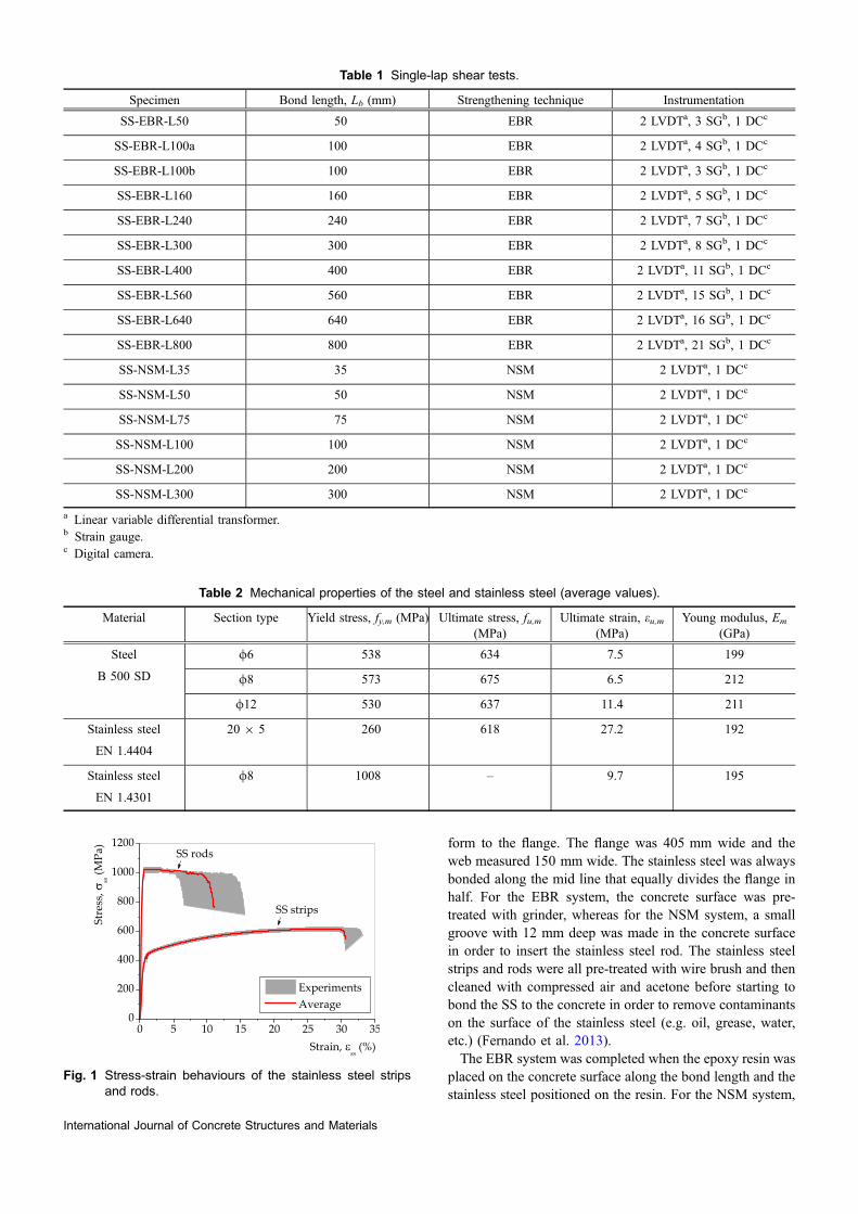
Thus, the slips obtained at the SS loaded end are eitherfrom Eq. (2) or from the DIC technique during the tests, i.e.the slip at x = Lb versus duration of the test is presented inFig. 7. As can be seen from this figure, the accuracy of theDIC technique with the slip derived from the strain gauges is

quite remarkable, especially in those specimens with largerbond lengths. However, a non-smooth slip distribution canbe easily seen from the specimens with shorter bond lengths,i.e. with a bonded length shorter than the effective bond

Fig. 6 Common failure modes observed from the single-lap shear tests: a EBR samples; and b NSM samples.

Table 3 Rupture loads and rupture modes observed in the specimens.

Specimen Bond length, Lb (mm) Rupture loads, Frup (kN) Failure mode

SS-EBR-L50 50 6.3 Type I

SS-EBR-L100a 100 12.8 Type II

SS-EBR-L100b 100 12.4 Type I

SS-EBR-L160 160 14.5 Type I

SS-EBR-L240 240 15.9 Type II


SS-EBR-L400 400 18.6 Type III




SS-NSM-L35 35 13.8 Type IV



SS-NSM-L100 100 40.1 Type V



Type I: adhesive rupture of the SS-to-resin interface; Type II: cohesive rupture within a surface layer of the concrete; Type III: cohesive rupturein concrete and adhesive within the SS-to-adhesive interface; Type IV: cohesive rupture within the concrete; Type V: rupture of the SS rod.


length, which induces a relevant noisy signal in determiningthe strains in the stainless steel.In terms of relative displacements between materials, the

Absolute Deviation (AD) and the Mean Absolute Deviation(MAD) between the DIC technique and the slips obtainedfrom the strain gauge measurements were calculated in eachtest according to:

AD ¼Xni¼1

sDIC0;i � s0;i�� ð3aÞ

and

MAD ¼ 1

n�Xni¼1

sDIC0;i � s0;i�� ð3bÞ

where s0 and s0DIC are the slips measured at x = 0 obtained

from Eq. (2) and from the DIC technique, respectively; andn is the number of measurements carried out during the test.The results showed that the specimens with the shortest bondlengths have the lowest MAD, whereas the specimens withthe longest bond lengths have the highest MAD. Thus, thelowest MAD was found in specimen SS-EBR-L50 with acalculated MAD of 0.002 mm and specimen SS-EBR-L560had the highest MAD of 0.019 mm.In terms of relative errors, the Absolute Percent Error

(APE) and the Mean Absolute Percent Error (MAPE) werealso determined according to:

APE ¼ 100�Xni¼1

sDIC0;i � s0;i��

s0;ið4aÞ

and

MAPE ¼ 100

n�Xni¼1

sDIC0;i � s0;i��

s0;i: ð4bÞ

The results showed that the MAPE tends to decrease withthe increase of the bond length adopted for the specimens.However, it is important to keep in mind that these resultsare very scattered but still, some tests showed that when thedisplacements increased the values for the MAPE tended todecrease. This may indicate that the use of the DIC tech-nique could be used if the displacements to be measured arenot too small. Therefore, the use of the DIC technique mayrequire some prudence and/or methodologies that should beconsidered for the experimental assessing of the bondbetween SS and concrete. In the following sections thoseaspects are highlighted and developed with the help of thesamples initially considered in this work.

4.2 Load–Slip ResponseThe load–slip response of the stainless steel bonded to

concrete will have different characteristics, depending if thebond length is longer or shorter than the effective bond

0 100 200 3000.00.10.20.30.40.50.60.7

Time, t (s)

Strain gaugesDIC

Slip

atx=0,s 0(m

m)

0.0000.0020.0040.0060.0080.010

Zoom

in

0.000.010.020.030.04

0 100 200 300 400 5000.00.10.20.30.40.50.60.7

Time, t (s)

Slip

atx=0,s 0(m

m)

SS-EBR-100a: SS-EBR-100b:Strain gauges Strain gaugesDIC DIC

Zoom

in

0.000.020.040.060.08

0 100 200 300 4000.00.10.20.30.40.50.60.7

Time, t (s)

Strain gaugesDIC

Slip

atx=0,s 0(m

m)

Zoom

in

(a) SS-EBR-L50 (b) SS-EBR-L100a/L100b (c) SS-EBR-L160

0.000.050.100.150.20

0 100 200 300 400 5000.00.10.20.30.40.50.60.7

Time, t (s)

Slip

atx=0,

s 0(m

m)

Strain gaugesDIC

Zoom

in

0 100 200 300 400 500 6000.00.10.20.30.40.50.60.7

Time, t (s)

Strain gaugesDIC

Slip

atx=0,

s 0(m

m)

0 50 100 150 200 250 3000.00.10.20.30.40.50.60.7

Time, t (s)

Strain gaugesDIC

Slip

atx=0,

s 0(m

m)

004L-RBE-SS)f(003L-RBE-SS)e(

0 50 100 150 2000.00.10.20.30.40.50.60.7

Time, t (s)

Strain gaugesDIC

Slip

atx=0,

s 0(m

m)

0 100 200 300 400 500 6000.00.10.20.30.40.50.60.7

Time, t (s)

Strain gaugesDIC

Slip

atx=0,

s 0(m

m)

0 50 100 150 2000.00.10.20.30.40.50.60.7

Time, t (s)

Strain gaugesDIC

Slip

atx=0,

s 0(m

m)

(d) SS-EBR-L240

(g) SS-EBR-L560 008L-RBE-SS)i(046L-RBE-SS)h(

Fig. 7 Comparison between the DIC technique and the strain gauges measurements through the slip at x = 0 versus timerelationship.


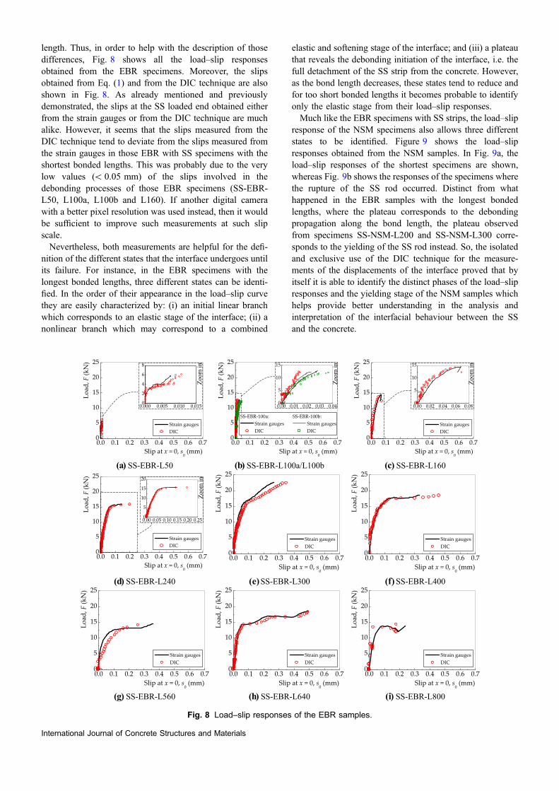
length. Thus, in order to help with the description of thosedifferences, Fig. 8 shows all the load–slip responsesobtained from the EBR specimens. Moreover, the slipsobtained from Eq. (1) and from the DIC technique are alsoshown in Fig. 8. As already mentioned and previouslydemonstrated, the slips at the SS loaded end obtained eitherfrom the strain gauges or from the DIC technique are muchalike. However, it seems that the slips measured from theDIC technique tend to deviate from the slips measured fromthe strain gauges in those EBR with SS specimens with theshortest bonded lengths. This was probably due to the verylow values (\ 0.05 mm) of the slips involved in thedebonding processes of those EBR specimens (SS-EBR-L50, L100a, L100b and L160). If another digital camerawith a better pixel resolution was used instead, then it wouldbe sufficient to improve such measurements at such slipscale.Nevertheless, both measurements are helpful for the defi-

nition of the different states that the interface undergoes untilits failure. For instance, in the EBR specimens with thelongest bonded lengths, three different states can be identi-fied. In the order of their appearance in the load–slip curvethey are easily characterized by: (i) an initial linear branchwhich corresponds to an elastic stage of the interface; (ii) anonlinear branch which may correspond to a combined

elastic and softening stage of the interface; and (iii) a plateauthat reveals the debonding initiation of the interface, i.e. thefull detachment of the SS strip from the concrete. However,as the bond length decreases, these states tend to reduce andfor too short bonded lengths it becomes probable to identifyonly the elastic stage from their load–slip responses.Much like the EBR specimens with SS strips, the load–slip

response of the NSM specimens also allows three differentstates to be identified. Figure 9 shows the load–slipresponses obtained from the NSM samples. In Fig. 9a, theload–slip responses of the shortest specimens are shown,whereas Fig. 9b shows the responses of the specimens wherethe rupture of the SS rod occurred. Distinct from whathappened in the EBR samples with the longest bondedlengths, where the plateau corresponds to the debondingpropagation along the bond length, the plateau observedfrom specimens SS-NSM-L200 and SS-NSM-L300 corre-sponds to the yielding of the SS rod instead. So, the isolatedand exclusive use of the DIC technique for the measure-ments of the displacements of the interface proved that byitself it is able to identify the distinct phases of the load–slipresponses and the yielding stage of the NSM samples whichhelps provide better understanding in the analysis andinterpretation of the interfacial behaviour between the SSand the concrete.

0.0 0.1 0.2 0.3 0.4 0.5 0.6 0.70

5

10

15

20

25

Load

,F(kN)

Slip at x = 0, s0(mm)

Strain gaugesDIC

0.000 0.005 0.010 0.0150

2

4

6

8

Zoom

in

0.0 0.1 0.2 0.3 0.4 0.5 0.6 0.70

5

10

15

20

25


Load

,F(kN)

SS-EBR-100a: SS-EBR-100b:Strain gauges Strain gaugesDIC DIC

0.00 0.01 0.02 0.03 0.040

5

10

15

Zoom

in

0.0 0.1 0.2 0.3 0.4 0.5 0.6 0.70

5

10

15

20

25Lo

ad,F

(kN)


Strain gaugesDIC

0.00 0.02 0.04 0.06 0.080

5

10

15

Zoom

in

0.0 0.1 0.2 0.3 0.4 0.5 0.6 0.70

5

10

15

20

25

Load

,F(kN)


Strain gaugesDIC

0.00 0.05 0.10 0.15 0.20 0.250

5

10

15

20

Zoom

in

0.0 0.1 0.2 0.3 0.4 0.5 0.6 0.70

5

10

15

20

25

Load

, F(kN)


Strain gaugesDIC

0.0 0.1 0.2 0.3 0.4 0.5 0.6 0.70

5

10

15

20

25

Load

, F(kN)


Strain gaugesDIC

0.0 0.1 0.2 0.3 0.4 0.5 0.6 0.70

5

10

15

20

25

Load

,F(kN)


Strain gaugesDIC

0.0 0.1 0.2 0.3 0.4 0.5 0.6 0.70

5

10

15

20

25

Load

, F(kN)


Strain gaugesDIC

0.0 0.1 0.2 0.3 0.4 0.5 0.6 0.70

5

10

15

20

25

Load

,F(kN)


Strain gaugesDIC

SS-EBR-L50 SS-EBR-L100a/L100b SS-EBR-L160

SS-EBR-L240 SS-EBR-L300 SS-EBR-L400

SS-EBR-L560 SS-EBR-L640

(a) (b) (c)

(d) (e) (f)

(g) (h) (i) SS-EBR-L800

Fig. 8 Load–slip responses of the EBR samples.


4.3 Slips Developed Within the InterfaceThe relative displacements between bonded materials (or

slips) developed along the bond length of the interface areanalysed next, in accordance to Eq. (2). Whether for the sakeof simplicity of the analysis or to avoid increasing the textunnecessarily, only two specimens were selected to be pre-sented, since the bond length of an interface has an importanteffect on its load–slip response: (i) the specimen with thelargest bond length; and (ii) the specimen with the shortestbond length. Also, both strengthening bond techniques arecontemplated in this analysis. Hence, Fig. 10 shows the slipdistributions obtained from the specimens SS-EBR-L50, SS-EBR-L800, SS-NSM-L35 and SS-NSM-L300. Furthermore,

the slips developed within the interface were calculatedtaking into consideration that:

s ¼ uss � uc ð5Þ

where uss and uc are the displacements in the stainless steeland in the concrete. Thus, since the DIC Correlate softwareprovides only the displacements, the slips measured usingthe DIC technique were calculated from the differencesbetween the displacements measured along a line thatembraces the bond length and another one that considers andmeasures the displacements along the concrete surface at thevicinity of the interface.

0.0 0.2 0.4 0.6 0.8 1.0 1.2 1.40

10

20

30

40

50

60

Load

,F(kN)

SS-NSM-L35 SS-NSM-L50SS-NSM-L75 SS-NSM-L100


0.00 0.05 0.10 0.15 0.200

10

20

30

40

Zoom

in

0.0 0.2 0.4 0.6 0.8 1.0 1.2 1.40

10

20

30

40

50

60

Load

,F(kN)


SS-NSM-L200SS-NSM-L300

(a) (b)

Fig. 9 Load–slip responses of the NSM samples with: a a short bond length; and b a long bond length.

0 5 10 15 20 25 30 35 40 45 500.000

0.005

0.010

0.015

0.020

Distance from the SS loaded end, x (mm)

DICFrom strain gauges

Slip,s

(mm)

0 5 10 15 20 25 30 350.00

0.05

0.10

0.15

0.20


DIC

Slip,s

(mm)

Short bond length, SS-EBR-L50 Short bond length, SS-NSM-L35

0 100 200 300 400 500 600 700 8000.00

0.05

0.10

0.15

0.20

0.25


1

1

3

DIC

From strain gaugesSlip,s

(mm)

2

1 2 3

0 50 100 150 200 250 3000.0

0.1

0.2

0.3

0.4

0.5


3

2

DIC:

Slip,s

(mm)

1

1 2 3

Key: 1 - same slip value s0 observed in specimen SS-EBR-L50 at failure; 2 - at approximately s0 = 0.1 mm; and 3 - at

the failure of the sample.

Key: 1 - same slip value s0 observed in specimen SS-NSM-L300 at failure; 2 - at the initiation of the yielding of the rods;

and 3 - at the failure of the sample. Long bond length, SS-EBR-L800 Long bond length, SS-NSM-L300

)b()a(

Fig. 10 Examples of the relative displacements obtained from the: a EBR samples; and b NSM samples.


The slips developed within the EBR interface chosen to bepresented in Fig. 10a correspond to the debonding loads ofthe specimens and in the case of the EBR sample with thelongest bonded length, an intermediate slip at x = 0 wasrandomly selected. Therefore, the distribution correspondingto ‘‘1’’ in Fig. 10a corresponds to the same slip at the SSloaded end when the debonding of the specimen SS-EBR-L50 occurred. In these cases, the results obtained either fromthe strain gauges or from the DIC technique are presented.Despite the noisy signal obtained from the DIC technique,the comparison between the two monitoring methods at leastallows us to check the capability of the DIC to follow thesame trend obtained from the strain gauges. Thereby, theresults shown in Fig. 10a indicate that the DIC technique iscapable of following the same slip distributions of thoseobtained from Eq. (2), i.e. with highest slips at the SS loadedend with a decrease of the slips towards the SS free end.The same criterion was followed in Fig. 10b to show the

slip distributions obtained from the NSM selected samples.However, the middle slip distribution in the specimen SS-NSM-L300 corresponds to the initiation of the yielding ofthe SS rod (see Fig. 10b). As can be seen from these results,a relevant discontinuity of the slip distribution can beobserved at the vicinities of the SS loaded end, which isexplained by the yielding of the SS rod. At the same time,the slip distributions corresponding to numbers ‘‘2’’ and ‘‘3’’are quite similar, which can be explained, once again, by theyielding of the SS rod outside of the bonded length. Thus,when the SS rod yields, the load transmitted to the SS rodremains the same and the slips along the bond length shouldremain almost unchanged from then. Consequently, thedisplacements increase elsewhere outside the SS-to-concreteinterface and the failure will also be localized there.

4.4 Axial Stresses and Strains Developedin the Stainless SteelAs mentioned above, the distribution of strains in the

stainless steel used on the EBR samples was obtained fromthe strain gauges. In addition to the measurements collectedfrom the strain gauges, the strains in the stainless steel werealso measured with the DIC technique. However, as shownin the previous subsection, the slips obtained from the DICtechnique are not quite smooth enough to obtain a smoothstrain distribution. Consequently, the axial stress distribu-tions obtained from both measurements are not much alike,as shown in Fig. 11a. Besides that, from Fig. 11 it can alsobe seen that the maximum axial stress in the stainless steelused on the EBR with SS specimens and measured by thestrain gauges is quite far away from its rupture value.Therefore, the mechanical properties of the stainless steelwere not fully used, which shows how inefficient the EBRtechnique is. However, using the DIC technique, the maxi-mum axial stress was, as expected due to its long bondedlength, registered in specimen SS-EBR-L800, which reached271.0 MPa at 190 mm away from the SS loaded end.In the NSM samples, the axial stress distributions are at

least consistent with what would be considered acceptable,i.e. the axial stresses developed in specimens SS-NSM-L35

are almost uniform and didn’t reached the yielding value ofthe SS rod. The debonding failure process of short bondedlengths is characterized by a slip distribution where there areno undeformed bonded regions (see Fig. 10). In addition,from the first derivative of Eq. (5) with respect to x andignoring the strains developed in the concrete, it could beconcluded that there are no regions where the strains couldbe zero unless, of course, precisely at the SS free end, wherethere are no assigned external loads to the stainless steel.In sum, and despite the differences and the procedures that

are needed to overcome the difficulties raised by the use ofthe DIC technique, the overall view of the results obtainedwith this monitoring technique is positive. In particular, thefact that several aspects observed in the experiments wereidentified and validated by the DIC technique. Even whenthe yielding of the SS rod was observed in specimen SS-NSM-L300, the DIC technique was capable of predictingthis as shown in the graph at the bottom of Fig. 11b.

5. Data Interpretation

In this section, the experimental results are discussed andanalyzed. Based on the experiments, the effective bondlength, i.e. the length beyond which the debonding loadcannot increase any more, is defined as the debonding loadvs. bond length graph. Moreover, the interfacial bond–sliprelationships obtained from the experiments both from theEBR system or NSM system are herein presented.

5.1 Definition of the Effective Bond LengthThe notion of effective bond length (Leff) of an interface is

widely assumed as the length beyond which the debonding(or maximum) load cannot increase with the increase of thebond length. In the literature, amongst other proposedmodels (e.g. Biscaia et al. 2013; Teng et al. 2001), theproposal made by Neubauer and Rostasy (Neubauer andRostasy 1997) can be used to estimate the debonding loadand the effective bond length of CFRP-to-concrete inter-faces. This has special importance in those cases where thebonded length is short and the effective bond length of theinterface is not ensured. Therefore, in order to predict theeffective bond length of the SS-to-concrete interfaces, themodel proposed by Neubauer and Rostasy (Neubauer andRostasy 1997) was used here. The results are shown inFig. 12, where the continuous black lines represent thecurves obtained by fitting Neubauer and Rostasy’s model(Neubauer and Rostasy 1997) with the experimental data bya minimization process of the maximum loads for the testedsamples with different bonded lengths. In the particular caseof the NSM system, the rupture observed from the twospecimens with the longest bond length was due to therupture of the SS rod and therefore, the limit of the curveobtained with the Neubauer and Rostasy’s model (Neubauerand Rostasy 1997) corresponds to the failure load of thestainless steel rods (48.5 kN), whilst the debonding load ofthe EBR system stayed only at 17.7 kN, which represents areduction of 63.5% when compared to the failure load of the


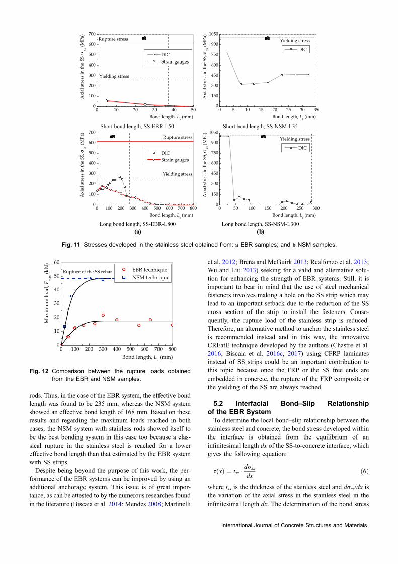
rods. Thus, in the case of the EBR system, the effective bondlength was found to be 235 mm, whereas the NSM systemshowed an effective bond length of 168 mm. Based on theseresults and regarding the maximum loads reached in bothcases, the NSM system with stainless rods showed itself tobe the best bonding system in this case too because a clas-sical rupture in the stainless steel is reached for a lowereffective bond length than that estimated by the EBR systemwith SS strips.Despite being beyond the purpose of this work, the per-

formance of the EBR systems can be improved by using anadditional anchorage system. This issue is of great impor-tance, as can be attested to by the numerous researches foundin the literature (Biscaia et al. 2014; Mendes 2008; Martinelli

et al. 2012; Brena and McGuirk 2013; Realfonzo et al. 2013;Wu and Liu 2013) seeking for a valid and alternative solu-tion for enhancing the strength of EBR systems. Still, it isimportant to bear in mind that the use of steel mechanicalfasteners involves making a hole on the SS strip which maylead to an important setback due to the reduction of the SScross section of the strip to install the fasteners. Conse-quently, the rupture load of the stainless strip is reduced.Therefore, an alternative method to anchor the stainless steelis recommended instead and in this way, the innovativeCREatE technique developed by the authors (Chastre et al.2016; Biscaia et al. 2016c, 2017) using CFRP laminatesinstead of SS strips could be an important contribution tothis topic because once the FRP or the SS free ends areembedded in concrete, the rupture of the FRP composite orthe yielding of the SS are always reached.

5.2 Interfacial Bond–Slip Relationshipof the EBR SystemTo determine the local bond–slip relationship between the

stainless steel and concrete, the bond stress developed withinthe interface is obtained from the equilibrium of aninfinitesimal length dx of the SS-to-concrete interface, whichgives the following equation:

s xð Þ ¼ tss �drssdx

ð6Þ

where tss is the thickness of the stainless steel and drss/dx isthe variation of the axial stress in the stainless steel in theinfinitesimal length dx. The determination of the bond stress

0 10 20 30 40 500

100

200

300

400

500

600

700Rupture stress

DICStrain gauges

Bond length, Lb(mm)

Axial

stress

intheSS

,SS(M

Pa)

Yielding stress

0 5 10 15 20 25 30 350

150

300

450

600

750

900

1050

DIC

Bond length, Lb(mm)

Axial

stress

intheSS

,SS(M

Pa)

Yielding stress

0 100 200 300 400 500 600 700 8000

100

200

300

400

500

600

700Rupture stress

DICStrain gauges

Bond length, Lb(mm)

Axial

stress

intheSS

,SS(M

Pa)

Yielding stress

0 50 100 150 200 250 3000

150

300

450

600

750

900

1050

DIC

Bond length, Lb(mm)

Axial

stress

intheSS

,SS(M

Pa)

Yielding stress

Short bond length, SS-EBR-L50 Short bond length, SS-NSM-L35

Long bond length, SS-EBR-L800 Long bond length, SS-NSM-L300)b()a(

σ

σσ

σ

Fig. 11 Stresses developed in the stainless steel obtained from: a EBR samples; and b NSM samples.

0 100 200 300 400 500 600 700 8000

10

20

30

40

50

60EBR techniqueNSM technique

Bond length, Lb(mm)

Max

imum

load

,Fmax(kN)

Rupture of the SS rebar

Fig. 12 Comparison between the rupture loads obtainedfrom the EBR and NSM samples.


between two consecutive strain gauges was accomplishedthrough the axial stressed developed in the stainless steel inwhich Eq. (1) was used. So, Eq. (6) can be rewritten as afunction of the difference between two consecutivecalculated axial stresses:

s xiþ1=2

� �¼ tss �

rss;iþ1 � rss;ixiþ1 � xi

ð7Þ

where (rss,i?1 - rss,i) and (xi?1 - xi) are, respectively, thestress in the stainless steel and the distance between twoconsecutive points. It is worth keeping in mind that Eq. (7)assumes, therefore, that the bond stresses developed betweentwo consecutive points are constant and, in order to ensure aprecise calculation of the bond stress, it is important to avoidhigh distances (xi?1 - xi) and distances shorter than 50 mmare recommended.The slip distribution is determined by Eq. (2) and the

bond–slip relationship is then determined by coupling thebond stress calculated from Eq. (6) and the average slipobtained from:

s xiþ1=2

� �¼ s xiþ1ð Þ þ s xið Þ

2ð8Þ

where s(xi?1) is the slip at point xi?1 and s(xi) is the slip atpoint xi.Figure 13 shows the interfacial bond–slip relationships

obtained from EBR with SS specimens with a bond lengthgreater than the effective bond length, i.e. over 235 mm. Ineach specimen, the different curves are presented and eachone corresponds to the mid-point of an interval between twoconsecutive strain gauges at a fixed distance from the SSloaded end. Despite some visible differences between sam-ples, the results show that the bond–slip relationships havesome points in common. For instance, for every singlespecimen, an initial increase of the bond stress is observeduntil a maximum bond stress is reached. This first stage isusually designated in the literature (e.g. Martinelli et al.2011; Dehghani et al. 2012; Biscaia et al. 2013, 2014; Xiaand Teng 2005) as an elastic stage. After this elastic stage, asoftening and nonlinear stage develops. The shape of thissoftening stage is not always the same and, for instance inspecimens SS-EBR-L240, SS-EBR-400 and SS-EBR-L800the softening stage seems to be quite symmetric with theelastic stage, whereas in the other samples the softeningstage decays quickly after the maximum bond stress valueand tends to be almost parallel to the x-axis as the slip withinthe interface approaches its ultimate value. The debondingstage, i.e. the stage with zero bond stress transfer, is notclearly observed in any of the EBR specimens studied here.Also the maximum bond stress and its corresponding max-imum slip developed within the interface was not always thesame.

5.3 Interfacial Bond–Slip Relationshipof the NSM SystemUnlike the EBR specimens with stainless steel which were

monitored with several strain gauges, the NSM specimenswere monitored only with the DIC technique. Hence, therelative displacement within the SS-to-concrete interfacemeasured with the DIC technique was the only informationgathered from the single-lap shear tests carried out in thiswork. For this reason, the methodology followed in theprevious section for determining the interfacial bond–sliprelationship of the EBR samples cannot be used in this caseof NSM specimens. The methodology followed in this sit-uation is described next and it was based on the strain vs.slip curve obtained from the test at the SS loaded end (@x = 0). This methodology was proposed by Dai et al. (Daiet al. 2005) and has been used since then by the authors withgood results (Biscaia et al. 2016c, 2017) to evaluate thebond–slip relationship developed within an FRP-to-concreteinterface. To determine the interfacial bond–slip relationship,this method requires that the slip and bond stress measure-ments at one specific point, which, in the present case,corresponds to x = 0. Hence, for the current NSM samples,the prediction of the interfacial bond–slip relationship of theSS-to-concrete interface begins by considering, once more,the equilibrium of a segment dx, leading to the followingequation (Biscaia et al. 2015a, b):

s xð Þ ¼ /ss

4� drssdx

ð9Þ

where /ss is the diameter of the stainless steel rod. Eq (9)can be rewritten as:

s xð Þ ¼ /ss

4� drssds

� dsdx

ð10Þ

where ds/dx is defined as the strain in the stainless steel,since the strains developed within the concrete are ignoreddue to their negligible values when compared to the strainsdeveloped in the stainless steel. Therefore, Eq. (10) can berewritten as a function of the axial stresses and strains in theSS according to:

s sð Þ ¼ /ss

4� drssds

� ess ð11Þ

where ess is the strain in the stainless steel. Eq (11) is thennumerically solved according to:

si sð Þ ¼ /ss

4� rss;iþ1 � rss;i�1

s0;iþ1 � s0;i�1� ess;i ð12Þ

where (rss,i?1 - rss,i-1) and (s0,i?1 - s0,i-1) are, respec-tively, the stress in the stainless steel and the slip betweenpoints i ? 1 and i - 1 of the stress versus slip curveobtained from the experiments at the SS loaded end. It isworth noting that for i = 0 the bond stress and the slip are,respectively, s0 = 0 MPa and s0 = 0 mm. Thus, from thestress versus strain behaviour of the stainless steel rods


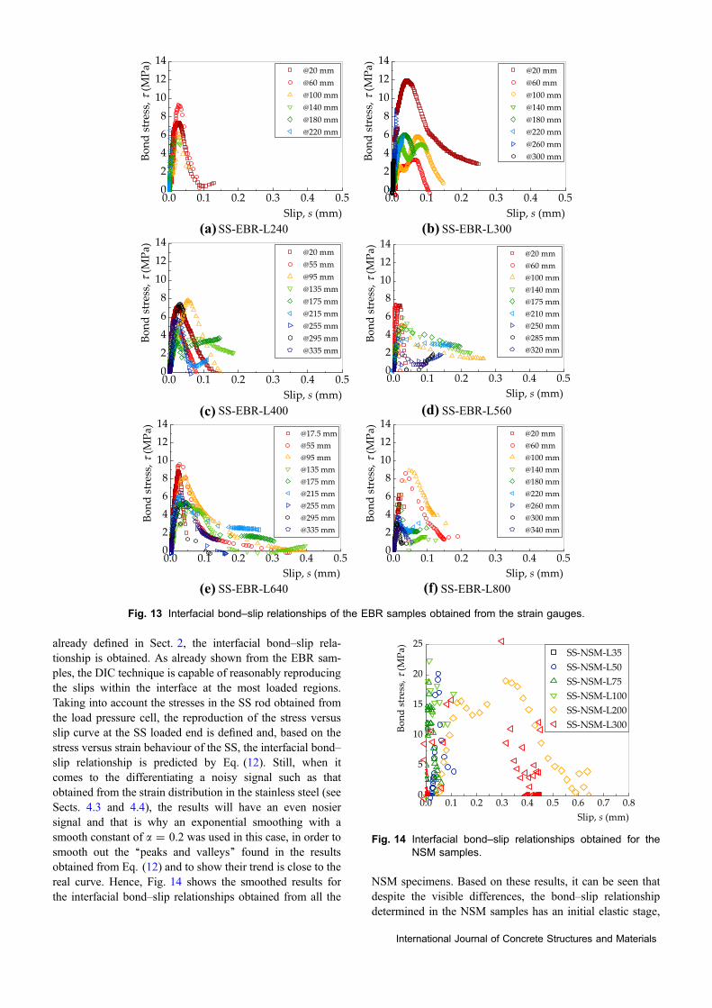
already defined in Sect. 2, the interfacial bond–slip rela-tionship is obtained. As already shown from the EBR sam-ples, the DIC technique is capable of reasonably reproducingthe slips within the interface at the most loaded regions.Taking into account the stresses in the SS rod obtained fromthe load pressure cell, the reproduction of the stress versusslip curve at the SS loaded end is defined and, based on thestress versus strain behaviour of the SS, the interfacial bond–slip relationship is predicted by Eq. (12). Still, when itcomes to the differentiating a noisy signal such as thatobtained from the strain distribution in the stainless steel (seeSects. 4.3 and 4.4), the results will have an even nosiersignal and that is why an exponential smoothing with asmooth constant of a = 0.2 was used in this case, in order tosmooth out the ‘‘peaks and valleys’’ found in the resultsobtained from Eq. (12) and to show their trend is close to thereal curve. Hence, Fig. 14 shows the smoothed results forthe interfacial bond–slip relationships obtained from all the

NSM specimens. Based on these results, it can be seen thatdespite the visible differences, the bond–slip relationshipdetermined in the NSM samples has an initial elastic stage,

(a)

(c) (d)

(e) (f)

(b)

Fig. 13 Interfacial bond–slip relationships of the EBR samples obtained from the strain gauges.

Fig. 14 Interfacial bond–slip relationships obtained for theNSM samples.


as well. However, at the end of this elastic stage, the bond–slip relationships in the NSM samples seems to show aplateau at a peak bond stress value and then, the bond stressdecays until it reaches a zero value. Thereof, bond–sliprelationships such as elastic with fragile rupture, rigid-plas-tic, rigid with linear softening or other reported in (Biscaiaet al. 2013) are herein excluded and a trapezoidal shape maydescribe better, even if approximately, the interfacial beha-viour shown in the NSM samples. In terms of the values ofthe nuclear points needed to define the bond–slip relation-ship, it can be stated that the maximum bond stress deter-mined from the NSM samples approximately reached20.0 MPa. Moreover, the maximum slip, i.e. the slip atmaximum bond stress, determined in the NSM samples isapproximately 0.2 mm more than the maximum slip calcu-lated in the EBR samples.

5.4 Interfacial Bond–Slip Relationships: EBRSystem Versus NSM SystemBased on the two NSM samples that failed due to the

rupture of the SS rod (specimens SS-NSM-L200 and SS-NSM-L300), it seems that the full detachment of the SS rodfrom the concrete occurs at a finite ultimate slip (sult),whereas in the EBR samples the separation between mate-rials takes place with a smoother transition. To help in thesecomparisons, Fig. 15 shows both curves where the bond–slip relationship determined either from the NSM samples orfrom the EBR samples are represented by areas limited bytheir minimum and maximum values. As can be seen fromFig. 15, the differences between both interfacial behavioursare different.Given the differences found here, the use of the NSM

bonding technique by itself is not sufficient to justify thosedifferences. Still, conjugated with the NSM bonding tech-nique, the use of ribbed stainless steel rods may justify suchdifferences in the bond stress transfer between samples withdifferent bonding techniques because the ribs increase thefriction within the interface leading to the improvement ofthe bond stress transfer between materials. In fact, in ModelCode 2010 (Federation Internationale du Beton 2010), theinfluence of the steel rib area is recognized as one of theaspects that significantly affects the bond–slip relationship.Moreover, a trapezoidal shape of the bond–slip relationship

to simulate the local bond behaviour between a ribbed steelrod and concrete is a possibility that is covered in ModelCode 2010 (Federation Internationale du Beton 2010).The mid-curves shown in Fig. 15 are intended to represent

the interfacial bond–slip relationships of each bondingtechnique studied here. Based on the maximum and mini-mum values obtained from each bonding technique, the mid-range curves in Fig. 15 are intended to cover a mid-rangevalue for the EBR and the NSM bonding techniques. Hence,the mid-range bond–slip relationship for the EBR bondingtechnique is defined according to (Popovics 1973):

s sð Þ ¼ smax � nn� 1ð Þ þ s

smax

� �n �s

smaxð13Þ

where smax is the maximum bond stress; smax is the slip atmaximum bond stress; and n is a constant to be defined inorder to approximate the shape of the bond–slip relationshipto the experimental results. The mid-range values needed forthe definition of Eq. (13) are: smax = 9.0 MPa,smax = 0.031 mm and n = 2.5. The mid-range bond–slipcurve for the NSM bonding techniques is defined accordingto:

s sð Þ ¼

smax

smax;1if 0� s� smax;1

smax if smax;1\s� smax;2smax

smax;2�smax;1� sult � s2ð Þ if smax;2\s� sult

0 if s[ sult

8>><>>:

ð14Þ

where smax,1 and smax,2 are, respectively, the slips at the endof the elastic stage and at the end of the constant stage; andsult is the ultimate slip, i.e. the slip beyond which no furtherbond transfer between materials is ensured. For the defini-tion of Eq. (14) shown in Fig. 15, a mid-range value for themaximum bond stress was found smax = 16.3 MPa and withslips smax,1 = 0.060 mm, smax,2 = 0.280 mm and sult =0.500 mm.

6. Conclusions

An experimental work was developed in order to study theperformance of stainless steel strips and rods bonded toconcrete. As well as the use of strain gauges to determine theinterfacial bond–slip relationship between the stainless steeland the concrete, the DIC technique was also used whichallowed a bonded area to be analysed instead of a local strainprovided by the use of single strain gauges. As an overviewof the results achieved, the following conclusions can bemade:

• The use of ribbed SS rods showed that it is possible toobtain the rupture of the rod if an appropriate bondedlength is used. In the present experimental work, it wasfound that for 200 mm the rupture of the SS rod isreached. Thereby, the premature debonding phenomenon

Fig. 15 Comparison between bond–slip curves.


of the SS rod is avoided and the mechanical properties ofthe SS rod are fully used;

• the EBR samples performed poorly when compared tothe NSM samples. In all the tests carried out, thepremature debonding of the SS strip was observed at astrain somewhat lower than its rupture value. In the EBRsamples with a short bond length, i.e. with a bondedlength shorter than the effective bond length, the ruptureoccurred within the SS-to-adhesive interface, whichmeans that the resin has poor properties for bondingSS strips. However, when the bond length of the SS-to-concrete interface increases, a mixed failure mode wasobserved with the separation of a thin layer of concretefrom the substrate with 2–3 mm of depth and, at thesame time, with an adhesive rupture within the SS-to-adhesive interface;

• the DIC technique can be used, although carefully, toevaluate the bond transfer between the SS and concrete.The displacements measured with the DIC technique andthe slips calculated from these results were reasonablywell estimated. Mainly when those values were greaterthan one tenth of a millimetre, the DIC proved to becapable of predicting the results fairly well. However, thenoisy signal obtained for the slips make it difficult todetermine the strains and bond stresses due to its higherorder, i.e. due to the first and second derivatives of theslips with respect to x (axis parallel to the bond length)for the calculation, respectively. Still, the methodologiesfollowed permitted the yielding of the SS rods in theNSM samples to be identified and allowed us to get a fairperspective of the strain distribution in the SS strip in theEBR samples;

• the DIC technique also allowed the load–slip distributionto be captured accurately. This weighs heavily in theevaluation of the bond between two materials because,based on the load–slip response, the interfacial behaviourcan be predicted. Thus, depending on the load–slipresponse until failure, the different stages that character-ize the bond–slip relationship can be estimated. Forinstance, an initial linear load–slip response means thatthe interfacial bond–slip relationship has a linear andelastic stage as well. Afterwards, the nonlinear load–slipresponse observed from the samples means that theinterfacial bond–slip relationship has a softening stage.This transition between the linear and the nonlinearload–slip response corresponds to a maximum bondstress value of the bond–slip relationship;

• The effective bond length of the EBR samples was235 mm, whereas the NSM samples had an effectivebond length of 168 mm, which represents 71.5% of thevalue obtained for the EBR samples;

• the bond–slip relationships obtained for the two types ofsamples studied here are different. In the EBR samples, apower function was able to describe a mid positioning ofthe experimental bond stresses (i.e. the correspondingmid-range values between the maximum and the mini-mum experimental bond stresses) obtained along theslips within the interface at the SS loaded end. However,

in the NSM samples, a trapezoidal shape to describe thebond–slip relationship was proposed to approximate theexperimental findings. Comparing the limit points ofboth bond–slip relationships, it can be concluded that themid-range maximum bond stress found for the NSMsamples reached 1.8 times of that found for the EBRsamples. In term of slips, the NSM samples had highervalues with the mid-range value of the ultimate slipdeveloped within the interface of the NSM samplesbeing approximately 0.5 mm, whilst an ultimate slip of0.4 mm was never exceeded in the EBR samples.

Acknowledgements

The first author of this work would like to express hisdeepest gratitude to Fundacao para a Ciencia e Tecnologiafor the partial financing of this work under the UNIDEMIStrategic Project PEst-OE/EME/UI0667/2014 and for thepost-doctoral grant SFRH/BPD/111787/2015. The secondauthor is also grateful to UNIDEMI for his scientificresearch grant under the Strategic Project UID/EMS/00667/2013.

Open Access

This article is distributed under the terms of the CreativeCommons Attribution 4.0 International License (http://creativecommons.org/licenses/by/4.0/), which permits unrestricted use, distribution, and reproduction in any medium,provided you give appropriate credit to the originalauthor(s) and the source, provide a link to the CreativeCommons license, and indicate if changes were made.

References

AG, & SPCRC. (2016). S&P Resin 220 (p. 2).

Aiello, M., & Leone, M. (2008). Interface analysis between

FRP EBR system and concrete. Journal of Composites Part

B: Engineering, 39(4), 618–626.

Akbar, I., Oehlers, D. J., & Ali, M. S. M. (2010). Derivation of

the bond–slip characteristics for FRP plated steel members.

Journal of Constructional Steel Research, 66(1–8),

1047–1056.

Almeida, G., Melıcio, F., Biscaia, H., Chastre, C., & Fonseca, J.

M. (2016). In-plane displacement and strain image analysis.

Computer-Aided Civil and Infrastructure Engineering,

31(4), 292–304.

Al-Mosawe, A., Al-Mahaidi, R., & Zhao, X.-L. (2015). Effect

of CFRP properties, on the bond characteristics between

steel and CFRP laminate under quasi-static loading. Con-

struction and Building Materials, 98, 489–501.

Arduini, M., Tommaso, A. D., & Nanni, A. (1997). Brittle

failure in FRP plate and sheet bonded beams. ACI Struc-

tural Journal, 94(4), 363–370.


http://creativecommons.org/licenses/by/4.0/

http://creativecommons.org/licenses/by/4.0/

Aykac, S., Kalkan, I., Aykac, B., Karahan, S., & Kayar, S.

(2013). Strengthening and repair of reinforced concrete

beams using external steel plates. Journal of Structural

Engineering, 139(6), 929–939.

Biscaia, H. C., Chastre, C., Borba, I. S., Silva, C., & Cruz, D.

(2016a). Experimental evaluation of bonding between

CFRP laminates and different structural materials. Journal

of Composites for Construction, 20(3), 04015070.

Biscaia, H., Chastre, C., Cruz, D., & Franco, N. (2017a).

Flexural strengthening of old timber floors with laminated

carbon fiber reinforced polymers. Journal of Composites

for Construction, 21(1), 04016073.

Biscaia, H. C., Chastre, C., Cruz, D., & Viegas, A. (2017b).

Prediction of the interfacial performance of CFRP lami-

nates and old timber bonded joints with different

strengthening techniques. Composites Part B Engineering,

108, 1–17.

Biscaia, H. C., Chastre, C., & Silva, M. A. G. (2013a). Non-

linear numerical analysis of the debonding failure process

of FRP-to-concrete interfaces. Composites Part B Engi-

neering, 50, 210–223.

Biscaia, H. C., Chastre, C., & Silva, M. A. G. (2013b). Linear

and nonlinear analysis of bond–slip models for interfaces

between FRP composites and concrete. Composites Part B

Engineering, 45(1), 1554–1568.

Biscaia, H. C., Chastre, C., Silva, C., & Franco, N. (2017c).

Mechanical response of anchored FRP bonded joints: A

nonlinear analytical approach. Mechanics of Advanced

Materials and Structures. https://doi.org/10.1080/

15376494.2016.1255812.

Biscaia, H. C., Chastre, C., Viegas, A., & Franco, N. (2015a).

Numerical modelling of the effects of elevated service

temperatures on the debonding process of frp-to-concrete

bonded joints. Composites Part B: Engineering, 70, 64–79.

Biscaia, H. C., Chastre, C., & Viegas, A. (2015b). A new dis-

crete method to model unidirectional FRP-to-parent mate-

rial bonded joints subjected to mechanical loads.

Composite Structures, 121, 280–295.

Biscaia, H. C., Cruz, D., & Chastre, C. (2016b). Analysis of the

debonding process of CFRP-to-timber interfaces. Con-

struction and Building Materials, 113, 96–112.

Biscaia, H. C., Franco, N., Nunes, R., & Chastre, C. (2016c).

Old suspended timber floors flexurally-strengthened with

different structural materials. Key Engineering Materials,

713, 78–81.

Biscaia, H. C., Micaelo, R., Teixeira, J., & Chastre, C. (2014).

Numerical analysis of FRP anchorage zones with variable

width. Composites Part B Engineering, 67, 410–426.

Bizindavyi, L., & Neale, K. W. (1999). Transfer lengths and

bond strengths for composites bonded to concrete. ASCE

Journal of Composites for Construction, 3(4), 153–160.

Blaschko, M., & Zilch, K. (1999). Rehabilitation of concrete

structures with CFRP strips glued into slits. In: ICCM-12,

I.—I.C.O.C. Materials. Paris, France: ICCM.

Brena, S. F., & McGuirk, G. N. (2013). Advances on the

behavior characterization of FRP-anchored carbon fiber-

reinforced polymer (CFRP) sheets used to strengthen

concrete elements. International Journal of Concrete

Structures and Materials, 7(1), 3–16.

Caggiano, A., Martinelli, E., & Faella, C. (2012). A fully-ana-

lytical approach for modelling the response of FRP plates

bonded to a brittle substrate. International Journal of Solids

and Structures, 49(17), 2291–2300.

Carrara, P., Ferretti, D., Freddi, F., & Rosati, G. (2011). Shear

tests of carbon fiber plates bonded to concrete with control

of snap-back. Engineering Fracture Mechanics, 78,

2663–2678.

CEN, EN ISO 6892-1:2009. (2009). Metallic materials. Tensile

testing—Part 1: Method of test at ambient temperature,

CEN.

CEN, NP EN 12390-3. (2003). Ensaios de betao endurecido:

Resistencia a compressao dos provetes de ensaio. Instituto

Portugues da Qualidade (in Portuguese).

Chastre, C., Biscaia, H., & Franco, N. (2017). Strengthening of

RC beams with post-installed steel bars or FRP composites.

Mecanica Experimental, 28, 39–46. (in Portuguese).

Chastre Rodrigues, C. Behaviour of steel-epoxy-soncrete con-

nection in structural elements. MSc thesis, Instituto Supe-

rior Tecnico; 209 pp. (in Portuguese).

Chastre, C., Biscaia, H. C., Franco, N., & Monteiro, A. (2016).

Experimental analysis of reinforced concrete beams

strengthened with innovative techniques. In: 41st IAHS

WORLD CONGRESS Sustainability and Innovation for the

Future (pp. 1–10), 13–16 September 2016, Albufeira,

Portugal.

Chen, J. F., Yuan, H., & Teng, J. G. (2005). Analysis of

debonding failure along a softening FRP-to-concrete

interface between two adjacent cracks. In: Chen, J. F., &

Teng, J. G. (Eds.), Proceedings of the International Sym-

posium on Bond Behaviour of FRP in Structures, BBFS

2005 (pp. 103–111).

Cruz, J. R., Borojevic, A., Sena-Cruz, J., Pereira, E., Fernandes,

P. M. G., Silva, P. M. and Kwiecien, A. (2016). Bond

behaviour of NSM CFRP-concrete systems: adhesive and

CFRP cross-section influences. In: Eighth International

Conference on Fibre-Reinforced Polymer (FRP) Compos-

ites in Civil Engineering (CICE2016).

Czaderski, C., Soudki, K., & Motavalli, M. (2010). Front and

side view image correlation measurements on FRP to

concrete pull-off bond tests. Journal of Composites for

Construction, 14(4), 451–463.

Dai, J., Ueda, T., & Sato, Y. (2005). Development of the non-

linear bond stress–slip model of fiber reinforced plastics

sheet-concrete interfaces with a simple method. Journal of

Composites for Construction, 9(1), 52–62.

De Lorenzis, L., Nanni, A., & Tegola, A. (2000). Strengthening

of reinforced concrete structures with near surface mounted

FRP rods. In: International Meeting on Composite Mate-

rials, PLAST 2000, Milan, Italy.

De Lorenzis, L., & Teng, J. G. (2007). Near-surface mounted

FRP reinforcement: An emerging technique for strength-

ening structures. Composites Part B Engineering, 38(2),

119–143.


http://dx.doi.org/10.1080/15376494.2016.1255812

http://dx.doi.org/10.1080/15376494.2016.1255812

Dehghani, E., Daneshjoo, F., Aghakouchak, A. A., & Khaji, N.

(2012). A new bond–slip model for adhesive in CFRP-steel

composite systems. Engineering Structures, 34, 447–454.

Eurocode 2 (EC2). (2004). Eurocode 2: design of concrete

structures—Part 1-1: General rules and rules for buildings.

EN 1992-1-1. December 2004.

Fawzia, S., Al-Mahaidi, R., & Zhao, X. L. (2006). Experimental

and finite element analysis of a double strap joint between

steel plates and normal modulus CFRP. Composite Struc-

tures, 75(1–4), 156–162.

Federation Internationale du Beton, FIB (2013).Model Code for

Concrete Structures 2010.

Fernando, D., Teng, J. G., Yu, T., & Zhao, X. L. (2013).

Preparation and characterization of steel surfaces for

adhesive bonding. Journal of Composites for Construction,

17(6), 04013012.

Fernando, D., Yu, T., & Teng, J. (2014). Behavior of CFRP

laminates bonded to a steel substrate using a ductile

adhesive. Journal of Composites for Construction, 18,

04013040.

Ferracuti, B., Savoia, M., & Mazzotti, C. (2007). Interface law

for FRP-concrete delamination. Composite Structures, 80,

523–531.

Franco, N., Chastre, C., & Biscaia, H. (2016). Analise do

desempenho da tecnica CREatE para reforco a flexao de

vigas de betao armado com armaduras de aco inoxidavel.

Encontro Nacional Betao Estrutural, 2–4 November, 2016

(pp. 1–10), Coimbra, Portugal. (in Portuguese).

Ghiassi, B., Xavier, J., Oliveira, D. V., & Lourenco, P. B.

(2013). Application of digital image correlation in investi-

gating the bond between FRP and masonry. Composite

Structures, 106, 340–349.

GOM Correlate software. Retrieved March 27 at http://www.

gom.com/3d-software/gom-correlate.html.

Gomes, A., & Appleton, J. (1999). Strengthening design of

concrete beams by addition of steel plates. In: EPMESC

VII: International Conference on Enhancement and Pro-

motion of Computational Methods in Engineering and

Science, 2–5 August 1999, Macao (pp. 657–666). Elsevier,

ISBN: 978-0-08-043570-1.

Harmon, T. G., Kim, Y. J., Kardos, J., Johnson, T., & Stark, A.

(2003). Bond of surface-mounted fiber-reinforced polymer

reinforcement for concrete structures. ACI Structural

Journal, 100(5), 557–564.

http://www.ncorr.com/. Retrieved March 27.

Jones, R., Swamy, R. N., Bloxham, J., & Bouderbalah, A.

(1980). Composite behaviour of concrete beams with

epoxy bonded external reinforcement. The International

Journal of Cement Composites, 2(2), 91–107.

Ladner, M. (1978). Field measurement on subsequently

strengthened concrete slabs. ACI Special Publication SP-

55, American Concrete Institute, Detroit (pp. 481–492).

Ladner, M. (1983). Reinforced concrete members with subse-

quently bonded steel sheets. IABSE Reports, 46, 203–210.

L’Hermite, R. (1977). Use of bonding techniques for reinforcing

concrete and masonry structures. Materiaux et Construc-

tion, 10(2), 85–89.

L’Hermite, R., & Bresson, J. (1967). Concrete reinforced with

glued plates. In: RILEM International Symposium, Syn-

thetic Resins in Building Construction, Paris (pp.

175–203).

Lorenzis, L., Miller, B., & Nanni, A. (2001). Bond of fiber-

reinforced polymer laminates to concrete. ACI Materials

Journal, 98(3), 256–264.

Martinelli, E., Czaderski, C., & Motavalli, M. (2011). Modeling

in-plane and out-of-plane displacement fields in pull-off

tests on FRP strips. Engineering Structures, 33,

3715–3725.

Martinelli, E., Napoli, A., Nunziata, B., & Realfonzo, R. (2012).

Inverse identification of a bearing-stress-interface–slip

relationship in mechanically fastened FRP laminates.

Composite Structures, 94(8), 2548–2560.

Mendes, R. M. V. (2008). CFRP strip anchorage systems to

reinforced concrete elements. MSc thesis, Instituto Superior

Tecnico. (in Portuguese).

Nakaba, K., Kanakubo, T., Furuta, T., & Yoshizawa, H. (2001).

Bond behavior between fiber-reinforced polymer laminates

and concrete. ACI Structural, 98(3), 359–367.

Neubauer, U., & Rostasy, F. S. (1997). Design aspects of con-

crete structures strengthened with externally bonded CFRP-

plates. In: Proceedings of the 7th International Conference

on Structural Faults and Repairs (Vol. 2, pp. 109–118).

Popovics, S. (1973). A numerical approach to the complete

concrete stress–strain relation for concrete. Cement and

Concrete Research, 3(5), 583–599.

Ramberg, W., & Osgood, W. R. (1943). NACA Technical Note

No. 902.

Realfonzo, R., Martinelli, E., Napoli, A., & Nunziata, B. (2013).

Experimental investigation of the mechanical connection

between FRP laminates and concrete. Composites Part B

Engineering, 45(1), 341–355.

Smith, S. T. (2010). Strengthening of concrete, metallic and

timber construction materials with FRP composites. In:

CICE2010—The 5th International Conference on FRP

composites in Civil Engineering, September 27–29, 2010,

Beijing, China.

Smith, S. T., & Teng, J. G. (2002). FRP-strengthened RC

beams. II: Assessment of debonding strength models.

Engineering Structures, 24, 397–417.

Swamy, R. N., & Jones, R. (1980). Behaviour of plated rein-

forced-concrete beams subjected to cyclic loading during

glue hardening. The International Journal of Cement

Composites, 2(4), 233–234.

Taljsten, B. (1997). Defining anchor lengths of steel and CFRP

plates bonded to concrete. International Journal of Adhe-

sion and Adhesives, 17(4), 319–327.

Teng, J. G., Chen, J. F., Smith, S. T., & Lam, L. (2001). FRP

strengthened RC structures. Chichester (England): Wiley.

Teng, J. G., Yuan, H., & Chen, J. F. (2006). FRP–to–concrete

interfaces between two adjacent cracks: Theoretical model

for debonding failure. International Journal of Solids and

Structures, 43, 5750–5778.

Van Germet, D. A. (1990). Repair and strengthening of rein-

forced concrete plates by epoxy-bonded steel plates. In:

Symposium on Structural Repairs/Strengthening by the


http://www.gom.com/3d-software/gom-correlate.html

http://www.gom.com/3d-software/gom-correlate.html

http://www.ncorr.com/

Plate Bonding Technique, 6–7 September 1990 (pp.

509–516), Sheffield, Great Britain.

Wan, J, Smith, S. T., & Qiao, P. Z. (2010). FRP-to-softwood

joints: An experimental investigation. In: CICE2010—The

5th International Conference on FRP composites in Civil

Engineering, September 27–29, 2010, Beijing, China.

Wan, J., Smith, S., Qiao, P.,& Chen, F. (2014). Experimental

investigation on FRP-to-timber bonded interfaces. Journal

of Composites for Construction, 18(Special Issue: 10th

Anniversary of IIFC), A4013006.

Wang, Z., & Vo, M. P. (2012). Short manual of the advanced

digital image correlation function in the MOIRE Software

Package (pp. 1–5). Retrieved March 27 at http://www.

dropbox.com/s/dp7a2hspee8neak/2DDIC_manual.pdf?dl=

0.

Wang, H. T., Wu, G., Dai, Y. T., & He, X. Y. (2016).

Determination of the bond–slip behavior of CFRP-to-

steel bonded interfaces using digital image correlation.

Journal of Reinforced Plastics and Composites, 35(18),

1353–1367.

Wu, Y. F., & Liu, K. (2013). Characterization of mechanically

enhanced FRP bonding system. Journal of Composites for

Construction, 17(1), 34–49.

Wu, W., & Yin, J. (2003). Fracturing behaviors of FRP-

strengthened concrete structures. Engineering Fracture

Mechanics, 70, 1339–1355.

Wu, Z., Yuan, H., & Niu, H. (2002). Stress transfer and fracture

propagation in different kinds of adhesive joints. Journal of

Engineering Mechanics, 128, 562–573.

Xia, SH and Teng, JG. Behaviour of FRP-to-steel bonded joints.

Proceedings of the International Symposium on Bond

Behaviour of FRP in Structures, Hong Kong, 2005.

Yao, J., Teng, J. G., & Chen, J. F. (2005). Experimental study on

FRP-to-concrete bonded joints. Composites: Part B, 36,

99–113.

Yu, T., Fernando, D., Teng, J., & Zhao, X. (2012). Experimental

study on CFRP-to-steel bonded interfaces. Composites Part

B Engineering, 43, 2279–2289.

Zhu, H., Wu, G., Shi, J., Liu, C., & He, X. (2014). Digital image

correlation measurement of the bond–slip relationship

between fiber-reinforced polymer sheets and concrete

substrate. Journal of Reinforced Plastics and Composites,

33(17), 1590–1603.


http://www.dropbox.com/s/dp7a2hspee8neak/2DDIC_manual.pdf%3fdl%3d0



Stainless Steel Bonded to Concrete: An Experimental ... · Abstract: The durability performance of...

Documents

Transcript of Stainless Steel Bonded to Concrete: An Experimental ... · Abstract: The durability performance of...