Staff Papers Series, P90-8, September 1990 - AgEcon...
32
Staff Papers Series Staff Paper P90-8 September 1990 ITERATIVE LEAST SQUARES ESTIMATION OF CENSORED REGRESSION MODELS WITH UNKNOWN ERROR DISTRIBUTIONS Yacov Tsur and Amos Zemel January 31, 1990 Current Version: September 1990 L5l Department of Agricultural and Applied Economics University of Minnesota Institute of Agriculture, Forestry and Home Economics St. Paul, Minnesota 55108
Transcript of Staff Papers Series, P90-8, September 1990 - AgEcon...

Staff Papers Series
Staff Paper P90-8 September 1990
ITERATIVE LEAST SQUARES ESTIMATION OF CENSORED REGRESSIONMODELS WITH UNKNOWN ERROR DISTRIBUTIONS
Yacov Tsur and Amos Zemel
January 31, 1990Current Version: September 1990
L5l
Department of Agricultural and Applied Economics
University of MinnesotaInstitute of Agriculture, Forestry and Home Economics
St. Paul, Minnesota 55108
Staff Paper P90-8 September 1990
ITERATIVE LEAST SQUARES ESTIMATION OF CENSORED REGRESSION
MODELS WITH UNKNOWN ERROR DISTRIBUTIONS
Yacov Tsur and Amos Zemel
January 31, 1990Current Version: September 1990
Staff papers are published without formal review with the Department of
Agricultural and Applied Economics.
The University of Minnesota is committed to the policy that all persons
shall have equal access to its programs, facilities, and employment
without regard to race, religion, color, sex, national origin, handicap,
age or veteran status.

Current version: September 1990
Iterative Least Squares Estimation of Censored Regression
Models With Unknown Error Distributions
Yacov Tsur and Amos Zemel
A simple and tractable algorithm to estimate censored
regression models with unknown error distribution is described.
The algorithm is based on a new empirical estimator of the
conditional expectation of the errors and is designed to yield
solutions to a fixed point equation via an iterative least
squares procedure. The resulting estimator is vN-consistent
and asymptotically normal.
The authors are grateful to L. Breiman for suggesting the empirical
conditional expectations and for his advice. They also wish to thank L.-F.
Lee, Y. Ritov, C. Sims, H. Ichimura and S. Thompson for helpful discussions.
Department of Agricultural and Applied Economics, University of Minnesota,
1994 Buford Avenue, St. Paul, MN 55108, USA. Supported by BARD Grant No.
US-1161-86.
Center for Energy and Environmental Physics, the J. Blaustein Institute for
Desert Research, Ben Gurion University of the Negev, Sede Boqer Campus, 84993,
Israel.

1
Iterative Least Squares Estimation of Censored Regression
Models With Unknown Error Distributions
Yacov Tsur and Amos Zemel
1. Introduction
Regression models with dependent variables which are incompletely
observed are pervasive. Restrictions on the observations occur, for example,
if a measuring device fails to give correct values beyond a given level, or
when the dependent variable, by its nature, is limited to a specific range
(e.g., can take only positive values). The literature is abundant with
further examples. Models describing such situations, known as censored
regression models, cannot be readily estimated using standard Least Squares
(LS) techniques due to the bias introduced by the censoring. When the error
distribution is specified the elimination of the bias is relatively simple; a
detailed treatment of this case is given in Breiman, Tsur and Zemel (1989).
The problem becomes involved in the more practical case of unknown error
distributions.
In this work we develop an estimator of the parameter vector of censored
regression models which does not require knowledge of the underlying error
distribution. We describe a simple, iterative algorithm to obtain this
estimator and show that it is consistent and asymptotically normal. Each
iteration consists of two steps: First, one fills in the missing data using
predictors based on the observations and on current parameter estimates.
Improved parameter estimates are then obtained by applying LS methods as if
no data are missing. The predictors used to fill in the missing data are
derived from estimators of the corresponding expectations of the errors
conditional on all available information. The construction of such predictors
in a way which generates consistent estimators, yet requires only few, simple
and fast computations is the key feature of our algorithm.

2
A similar procedure was suggested by Buckley and James (1979) and further
investigated by James and Smith (1984) and by Ritov (1990). Our procedure
differs in the way the empirical estimators of the error conditional
expectations are evaluated. The proposed empirical estimators were also used
by Lee (1988) in the context of semiparametric truncated regression models.
Other approaches to estimate censored regression models without
specifying the error distribution have been discussed by Powell (1984, 1986),
Duncan (1986), Fernandez (1986), Horowitz (1986), Nawata (1990), Tsiatis
(1990), and Ritov and Fygenson (1990). The estimators studied in these works
were shown to be consistent and asymptotically normal. Some of them, however,
are not easy to implement and their application to data may become
computationally cumbersome.
When the EM algorithm of Dempster, Laird and Rubin (1977) is applied to a
censored regression model with Gaussian errors, one obtains an iterative LS
procedure, where in each iteration the missing data are replaced by their
expectations conditional on all available information (Tsur (1983)). The
resulting estimator was shown to maximize the likelihood function, hence it is
consistent and efficient. It is of interest, then, to find out whether such
an iterative LS procedure maintains desirable large sample properties when
applied to models with non normal (but known) distributions. Breiman, Tsur
and Zemel (1989) answered this question in the affirmative and further showed
that this iterative LS procedure (referred to as the EP algorithm) possesses
excellent convergence properties.
Proceeding along this line of thought, the next quest to pursue concerns
the properties of a similar procedure in which distribution-free empirical
estimates of the error conditional expectations are employed. Indeed this is
the main theme of this work. Analyzing the algorithm based on the new
empirical conditional expectations, we find that the governing equations are

3
very similar (asymptotically) to those corresponding to the case of known
error distributions, and that the distribution-free EP estimator is consistent
and asymptotically normal.
We begin, in Section 2, by describing the EP algorithm and define the EP
estimator. In its strict form, the estimator is defined as a solution of a
fixed point equation. Due to discontinuities in the empirical estimates, such
a solution may not always exist in finite samples. We thus generalize the
solution concept from a point to a neighborhood that shrinks (at a rate faster
than 1//N) with the sample size N and prove, in Section 3, the existence of a
/N-consistent solution. Consistency of the EP estimator, then, requires the
identification of the consistent root if more than one solution exists. The
selection of this root is based on a minimization criterion recently proposed
by Lee (1988) for the truncated case. Finally, we show that the EP estimator
is asymptotically normal and derive its limiting covariance matrix.

4
2. The EP Algorithm and Estimator
We consider a model in which the data (yi,xi) are generated by the
mechanism
yi - MAX(O,ao+xi.o+ui), i-1,2,...,N
where yi are observed scalars, xi are iid K-dimensional observed vectors, ao
is an unknown intercept parameter, So is a K-dimensional vector of unknown
slope parameters to be estimated, ui are iid error terms distributed according
to some unknown cdf F with E(ui) - 0, and N is the number of measurements.
The value (Yi-O) indicates that yi is missing, otherwise Yi>0.
Let x - xi - x, where x - Ex(xi), be the shifted regressors expressed as
deviations from the mean. Let e. - u. + ao + x'po be the shifted errors with
mean E{e.) e - ao + x'io and cdf F (z) - F(z-e). Let zi --o - x'.Po and
zi- -x';o, so that zi - Zi - e. Thus, recalling ei - u + e, one has~. Thus, recaling 61 1
F (z) - F(zC) and E(e|e<zi ) - E(ulu<z t) + e. Because F is always evaluated
at a shifted argument we suppress the subscript e without risking confusion.
Denoting the index sets corresponding to the observed and missing cases
by M - (i: z° < ei) i (i: yi > 0) and M - (i: z. > ei) - (i: yi - 0), thei 1 1 1 1
model can be equivalently presented as
x'fi o + ei ; iEM +
yi - , i-1,2,..,N. (2.1)i 0 ;f iM(2.1)
Model (2.1), expressed in terms of the shifted regressors and errors, will be
referred to as the shifted model. The N by K matrix whose i'th row is x'i is
denoted by X and X is its partition to the observed cases, i E M+.
The EP algorithm is an iterative procedure to estimate the slope vector
Po. Each iteration consists of two steps: an Expectation (E) step and a
Projection (P) step. The idea is to replace the missing values yi, i E M , by
their expectations, using all the available information including the
parameter estimate obtained in the previous iteration. These values for yi
5
are then employed to find an improved estimator for Po.
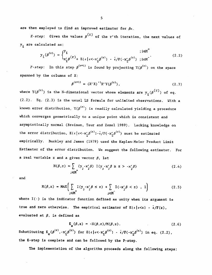
(r)E-step: Given the values (Br) of the r'th iteration, the next values of
yi are calculated as:
~~Y~~~~~i ~;i-M+yi(P 1(r)) -{yi r) . (2.2)
x'I )+ E{eIl<-x'.p r - e/F(-xi' ) ;ieM
P-step: In this step h(r+l) is found by projecting Y(P)) on the space
spanned by the columns of X:
f(r+l) - (X X) X, y(P)), (2.3)
where Y(fir)) is the N-dimensional vector whose elements are y.( (r)) of eq.
(2.2). Eq. (2.3) is the usual LS formula for unlimited observations. With a
known error distribution, Y((r)) is readily calculated yielding a procedure
which converges geometrically to a unique point which is consistent and
asymptotically normal (Breiman, Tsur and Zemel 1989). Lacking knowledge on
the error distribution, E{(ee<-xi.(r) )-e/Fx~((r)) must be estimated
empirically. Buckley and James (1979) used the Kaplan-Meier Product Limit
Estimator of the error distribution. We suggest the following estimator. For
a real variable z and a given vector f, let
H(i,z) - (y.-x'P) I(y -x' > z > -x'P) (2.4)
jEM
and
M(9,z) - MAX ( I(y -x'fi < z) + I(-x'P < z) , 1) (2.5)
jieM jEM
where I(-) is the indicator function defined as unity when its argument is
true and zero otherwise. The empirical estimator of E(ele<z) - e/F(z),
evaluated at f, is defined as
E e(,z) - -H($,z)/M(,,z). (2.6)
Substituting Ee ((r,-x) ()) for E(e|l<-x (r)) - e/F(-xp (r)) in eq. (2.2),
the E-step is complete and can be followed by the P-step.
The implementation of the algorithm proceeds along the following steps:

6
1) Form the shifted regressor matrix X using the mean i x a/N as an estimate
of x.
2) Set (o), an initial value for the parameter vector.
3) Fill in the missing yi values as given by eq. (2.2) using E e(,-x'i) with
the current f-estimate (E-step).
4) Update P according to eq. (2.3) (P-step).
5) Return to step 3 unlessK
I(r+l) (r) 112 - ((r+l)- (r) 2
decreases below some predetermined convergence requirement.
6) Once the convergence criterion is satisfied, adopt the last value of $ as
the final estimate.
The limit of this iterative process is the EP estimator and may be
considered as the solution to the Fixed Point Equation (FPE)
0 - (X'X)-1 X'Y(P). (2.7)
The discontinuities (with respect to P) in E may cause situations in
which the FPE does not have a solution (the same problem was noticed by
Buckley and James (1979) for their estimator). Practical experience shows
that the EP algorithm then settles to oscillations among several fixed values
instead of converging to a unique fixed point. Once this situations has been
identified, the iterations are terminated; the criterion to select the proper
oscillation point is described below. A related ambiguity stems from the
theoretical difficulty in proving the asymptotic uniqueness of the solution of
the FPE. Although it is shown in the next section that the FPE must have a
consistent root, it is not clear that every solution is indeed consistent.
One can, however, identify the consistent root among a given set of possible
solutions (arrived at, for example, by starting the algorithm at different
initial values in a situation where such non uniqueness occurs), according to
the following criterion: Let

7
Mc( ,z) - I(yj-x' 2 z > -x'P) (2.8)
jeM
and
Ee (,z) - H(P,z)/Mc(,z) (2.9)ec C
be an estimator of E(e|e>z) (cf. Eq. 2.6). Define also
Qe() (yi - x+( - Eec (p2-Ixi.)/N (2.10)
i M
and evaluate Qe for every solution of the FPE. The root corresponding to theN
minimum value of Q is adopted as the EP estimate.N
The FPE is here presented as a result of a specific iterative procedure.
In the following section the solutions of this equation are analyzed without
reference to the particular algorithm used to obtain them. Thus, the results
presented below are valid for any method of solution, yet the EP algorithm
proposed here is particularly convenient for numerical implementation.
8
3. Asymptotic properties
We derive in this section the consistency and asymptotic normality of the
EP estimator. The analysis is based on properties of the FPE. As explained
above, this equation does not necessarily have a solution for every finite
sample. Therefore, the term "solution to the FPE" must be generalized,
allowing deviations that diminish as the sample size N increases. We show the
existence of a consistent and asymptotically normal "generalized solution" to
the FPE, and verify that the EP estimator coincides with this particular
solution. Aiming at simplicity, the derivations are based on a set of
assumptions which are somewhat restrictive but clarify the proofs. In
general, we assume uniform bounds when weaker moment conditions may suffice.
Several generalizations are possible, but the investigation of the minimal
conditions under which the results hold will be carried out elsewhere.
In addition to the standard condition that the regressors are
statistically independent of the errors, we require:
Assumption 1:
(i) xi are iid with a distribution having a bounded support.
(ii) X'X/N is uniformly positive definite (upd).
(iii) The distribution of z -x'po, induced by the distribution of xi, has
a bounded density.
(iv) For z restricted to the bounded support of zi, the error distribution
is bounded: 1 - 6 > F(z) > 6 for some 1 > 6 > 0, and the density
f(z) -F'(z) is bounded.
(This implies that the functions E(z) - E(e|e<z) and E'(z) - dE/dz are also
bounded.)
(v) E(e4 ) < o.
The empirical conditional expectation E is the key ingredient of thee

9
algorithm. We begin by deriving an important consistency property of Ee . Let
N
z. -x '. and N(P,z) - I(z < z). For F(z) > 0, the following result holds:
Theorem 1: E (Po,z) -H E(e|e<z) - e/F(z) provided N(oo,z)->c .
(All proofs are presented in the appendix.) Theorem 1 claims that for the
true parameter, Po, the evaluation of E at any z within the support of z.e 1
provides a consistent estimator of the quantity required to fill in the
missing y-values (cf. Eq. (2.2)). This consistency property has motivated
definitions (2.4)-(2.6) of the empirical conditional expectations. Note that
the relevant sample size is N(P,z) rather than N. This technical difficulty
is addressed throughout the derivations.
Using Theorem 1 we next show that Po is an asymptotic solution of the FPE.
The notation 0 (1) is used to denote a variable having a mean and a varianceqm
which are o(l) and 0(1), respectively. A variable is o (1) if both its mean
and variance are o(l). Let W(P) - Y(p)-Xp and observe that, since X'X/N is
upd, 0(p)-X'W(P)/VN can serve as a measure of the degree of precision to which
the FPE is satisfied. At Po, 4 assumes a particularly simple form. Let
Si eiI(i>zi) + (E(zi)-e/F(zi))I( fizi); ai-Var(si), Z be the N by N
diagonal matrix with elements ai and V - E (X'ZX/N). Assumption 1 ensures
that V exists and is positive definite. Then, we can prove
Theorem 2: Under Assumption 1, O(Po) - N(0,V).
Theorem 2 immediately implies that Po is an asymptotic solution of the FPE:
Corollary: Under Assumption 1, vN((X'X)-X'Y(Bo) - Po) - Om(l).
Moreover, Theorem 2 plays a key role in the derivation of the asymptotic
distribution of the EP estimator (cf. Theorem 6 below).
The observation that Po solves the FPE asymptotically suggests the
existence of solutions that approach Po as N-> '. However, as mentioned in

10
Section 2, the FPE may not have an exact solution for any finite sample.
Nonetheless, the solution concept can be slightly generalized to vectors that
satisfy the FPE to a better approximation than Po. Then, as shown below, it
is possible to verify the existence of a consistent and asymptotically normal
"generalized solution", which coincides with the EP estimate.
Definition: A vector p is a solution to the FPE if +(p) - o (1), that is ifqm
VN((X'X) -1X'Y() - P)- 0.qm
Since (fl9o) - 0 (1), po does not qualify as a solution and we need someqrn
preparations to show that generalized solutions indeed exist.
Let x. ,X and z. represent respectively xi, X and z° after ordering
the regressors xi according to their projections on Po:
1 ~j oi < j = z < z.1 j
Define the K by K matrix
0 - x(o)' r(I-A)X(°)/N. (3.1)N
Here r is an N by N diagonal matrix with
.ii - -(z ) FiE' + 1 - Fi + fi/Fi' (3.2)
where Fi, E' and f. are evaluated at zi° ) and A is the N by N matrix
1 o 0 o ,... . a1 2 1/2 0 0 0 0
A - . 1/ 3 1/3 0 0 0 (3.3)
'i/ n-1) 1/(n-l) 1/(n-l) 1/(n-l)... 1/(n-l)
The ordering has been introduced in order to specify A as a fixed (non
random) matrix. Without ordering, the rows of A would have to be permuted
according to the (random) order of z °
We are now ready to establish the following result:
Theorem 3: Under Assumption 1, for any p such that AP - f-fo - O(1/IN),
AO - +(p) - O(Po) - -f0 VNAP + oqm(l).
According to Theorem 3, the FPE is essentially linear in a small region around
According to Theorem 3, the FPE is essentially linear in a small region around

11
pa and the matrix 0 is nothing but the derivative of -(fiP)/VN with respect toN
P. The condition needed to guarantee the existence of a consistent solution
to the FPE is therefore equivalent to the condition required for nN to be
uniformly nonsingular. In fact, a solution can (in principle) be constructedA
explicitly, using the Newton-Raphson value PN = 8P + 0nN1 (o)/VN. The matrix
N plays here the role played by X'X/N in the uncensored regression model.N
For censored regression with a known error distribution, the corresponding
matrix is X'rX/N (Breiman, Tsur and Zemel, 1989). The matrix A represents,
therefore, the modifications introduced by the use of the empirical
conditional expectation.
The explicit form of N can now be used to investigate its properties,N
taking into account the random nature of X. (It so happens that the matrix
corresponding to 0 in the unshifted model becomes singular as N -, o; thisN
explains the use of the shifted model.)
As mentioned above, the cost of having a non-random A is the need to
order xi, which disturbs the independence among the rows of X. Therefore, it
is expedient to introduce a normalized regressor matrix Z - . on which
the effect of the ordering is restricted in the following sense: the elements
of the first column retain the original ordering of zo whereas the elements of
the other columns, while not yet independent, are uncorrelated with zero
means.
Let A - E(X'FX/N), Co - 11A1/2oli and b - A1/2Po/Co. Construct K-l unit
vectors bz....b such that the K by K matrix B - (b ....bK) is orthogonal.
The normalized regressor matrix is given by Z -XA-1/2B. It is verified that
fil - -x'io/Co. We denote the cdf of these quantities, induced by the
distribution of xi, by F (.). The definition of Z is meaningful, and its
desirable properties are guaranteed if the following assumptions hold:
12
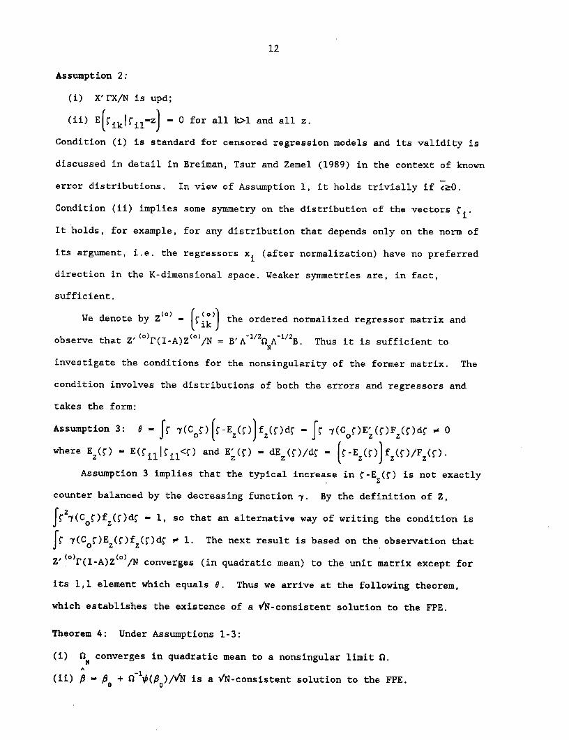
Assumption 2:
(i) X'rX/N is upd;
(ii) E(ikl il -z) - 0 for all k>l and all z.
Condition (i) is standard for censored regression models and its validity is
discussed in detail in Breiman, Tsur and Zemel (1989) in the context of known
error distributions. In view of Assumption 1, it holds trivially if e20.
Condition (ii) implies some symmetry on the distribution of the vectors fi.
It holds, for example, for any distribution that depends only on the norm of
its argument, i.e. the regressors xi (after normalization) have no preferred
direction in the K-dimensional space. Weaker symmetries are, in fact,
sufficient.
We denote by Z(0) - (fik) the ordered normalized regressor matrix and
observe that Z' ()r(I-A)Z(°)/N = B'A-1/2' A-1/'B. Thus it is sufficient toN
investigate the conditions for the nonsingularity of the former matrix. The
condition involves the distributions of both the errors and regressors and
takes the form:
Assumption 3: - Jr -(C r) (r-E(f)f f,(d- Jr -y(Cr)E' ()F(O)dS v 0
where Ez(S) - E(fill il<) and E'(f) - dE(f)/df - (f-ES ()]f (f)/F(f).
Assumption 3 implies that the typical increase in f-Ez(f) is not exactly
counter balanced by the decreasing function 7. By the definition of Z,
f 2y(C o)f (f)d - 1, so that an alternative way of writing the condition is
If (COf)Ez(f)fz(r)df - 1. The next result is based on the observation that
Z'(°)r(I-A)Z(°)/N converges (in quadratic mean) to the unit matrix except for
its 1,1 element which equals 6. Thus we arrive at the following theorem,
which establishes the existence of a VN-consistent solution to the FPE.
Theorem 4: Under Assumptions 1-3:
(i) nN converges in quadratic mean to a nonsingular limit n.A
(ii) P - P + -lVb(0 )/VN is a VN-consistent solution to the FPE.

13
In view of Theorem 4, the EP algorithm (or any alternative method of
solving the FPE) seems to provide a promising procedure for generating
consistent estimators. Indeed, if one starts at a S-value which is close
enough to 3o, the linear nature of (fp) in that region ensures that the
consistent solution will be found. However, the results presented so far
discuss local properties only, and do not rule out the existence of solutions
which are remote from Po. In order to establish consistency one needs global
results that ensure uniqueness (to O(1/VN)) of the solution. For this
purpose, too, the n matrix formalism might prove useful since a generalization
of Theorem 3 to arbitrary AP entails consistency if the generalized 0 is
nonsingular. Indeed, for certain simple distributions explicit expressions
for this matrix could be derived. The identification of sufficient conditions
for nonsingularity is, however, more involved.
An alternative approach is based on recent results obtained by Lee (1988)
for truncated regression models. Using a smooth version of the empirical
conditional expectations, Lee (1988) constructed a consistent estimator for
the truncated model by minimizing a sum of mean-corrected squared errors.
Obviously, Lee's method can be applied also to censored models. However,
smoothing procedures tend to complicate the computations and an attractive
feature of the EP algorithm is lost.
In the censored case it is preferable, therefore, to employ the EP
algorithm to obtain solutions to the FPE. When more than one solution is
found, the selection of the consistent root proceeds as described in Section
2. Let Fc(z) - 1 - F(z); Ec(z) - E(ele>z) and EC (z) - E(e2 le>z). An
empirical estimator to Elc(z) is defined in eq. (2.9) and used to construct
the objective function Q (p) in eq. (2.10). Taking expectation over ej, weN 3
define the following quantities:
hj(iz) - FC(z + A)I(z > zj)(Elc( + A) -A );
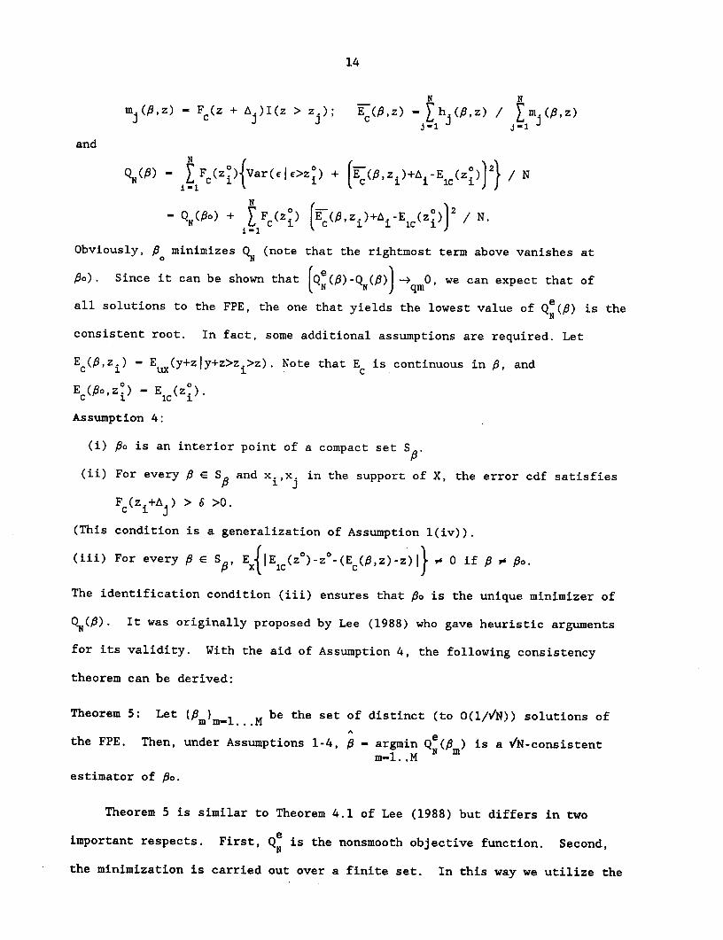
14
N Nm.j(,z) - Fc(Z + Aj)I(z > ); EC(Pz) - h (9,z) / Emj(,z)
j-E 1 j -1
and
QN) - E F (z )Var(c|>z0) + E('zi)+i-Elc(Z 2) NC i \ J J E E>Zo
- QN(B) + N F(zc ) (Ec( ,zi)+A2i- l )) / N
Obviously, Po minimizes QN (note that the rightmost term above vanishes at
Po). Since it can be shown that (Q ()-Q (3)) -q 0, we can expect that of
all solutions to the FPE, the one that yields the lowest value of QN () is theN
consistent root. In fact, some additional assumptions are required. Let
Ec(U,zi ) - E (y+zly+z>zi>z). Note that E is continuous in f, and
Ec(o,zi) - Ec(Z').
Assumption 4:
(i) po is an interior point of a compact set S .
(ii) For every E( SP and xi,xj in the support of X, the error cdf satisfies
Fc (zi +A ) > 6 >0.
(This condition is a generalization of Assumption l(iv)).
(iii) For every P E SP, E{ Elc(z°)-z°-(E c(,z)-z) } 0 if P * po.
The identification condition (iii) ensures that Po is the unique minimizer of
QN($). It was originally proposed by Lee (1988) who gave heuristic arguments
for its validity. With the aid of Assumption 4, the following consistency
theorem can be derived:
Theorem 5: Let (m)m-1 .M be the set of distinct (to O(1/VN)) solutions ofA
the FPE. Then, under Assumptions 1-4, P - argmin QN(fm) is a / N-consistentm-l..M
estimator of Po.
Theorem 5 is similar to Theorem 4.1 of Lee (1988) but differs in two
important respects. First, QN is the nonsmooth objective function. Second,
the minimization is carried out over a finite set. In this way we utilize the

15
global properties of Lee's procedure while retaining the computational
simplicity of the EP algorithm.
Applying Theorems 3 and 4 to the VN-consistent P givesA ^
~(o) - -AX + o (1) - nVN(P - Bp) + o (1) - C/N(P - 8o) + o (1).
According to Theorem 2, k(fo) ) N(O,V) while Theorem 4 ensures that n is
nonsingular. Thus we arrive at
A
Theorem 6: Under Assumptions 1-3, VN(c - Do) N(O0O'O ' 1 ).
16
4. Concluding remarks
A major problem in the study of estimation procedures of censored or
truncated regression models which are robust with respect to the specification
of the error distribution is the need to establish asymptotic uniqueness of
the solutions. Many of the estimators are defined as the extremum points of
some underlying objective function. Estimators of this kind benefit from the
well-developed techniques to analyze extremum estimators, and the conditions
under which they are consistent (i.e., the true parameter is asymptotically a
unique extremum point) are usually identified. However, these estimators tend
to be computationally cumbersome, since they entail optimization of objective
functions which are either non-differentiable or require smoothing procedures.
A different class of estimators is defined by fixed points of some
iterative estimation procedure. These estimators are often more tractable
computationally, but it is more difficult to verify that their estimation
equations have unique solutions. (See, for example, Ritov (1990) on the
properties of the Buckley and James (1979) estimator). Under favorable
conditions, the fixed point solutions are also the extremum points of
objective functions. The EP estimator, for example, maximizes the likelihood
function when the errors have normal distribution (Tsur, 1983) and a convex
generalized sum-of-squares function for non-normal, but known, error
distributions (Breiman, Tsur and Zemel, 1989). For the general,
distribution-free, case the construction of a proper objective function is
more difficult.
These observations lead us to the structure of the EP estimator proposed
in this work. It is produced by an iterative algorithm which first locates
the solutions of the estimation equation, then selects the consistent root if
multiple roots are found. The second stage establishes the connection to the

17
extremum estimators and ensures the asymptotic uniqueness of the solution.
However, both stages employ the simple, discontinuous empirical conditional
expectations, permitting fast and easy numerical implementations.
The insistence on the simple empirical conditional expectation entails a
certain complication in the theoretical analysis: the relevant sample size for
the empirical estimators is only a fraction of N. Thus, the convergence of
these estimators is not uniform. This situation is in contrast to Lee's study
(1988), where smoothing and trimming procedures ensure uniform convergence and
simplify the subsequent analysis. For the EP case, however, it is found that
the relevant correction terms are typically O(logN/VN) and do not affect the
asymptotic properties of the estimator.
18
Appendix: Proofs of theorems
The following result is central to the analysis.
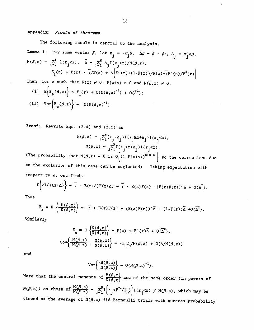
Lemma 1: For some vector A, let zj - -x'., A- - , - 3o, A. xjA,N - N J J J '
N(f,z) - z I(zj<z), A - Z AI(zj<z)/N( ,z),j-1 j1 j
E (z) - E(z) - e/F(z) + A(E'(z)+(l-F(z))/F(z)+eF'(z)/F 2(z)
Then, for z such that F(z) o 0, F(z+A) o 0 and N(9,z) v 0:
(i) E{Ee( ,z)} - El(z) + O(N(P,z)-) + 0(A2);
(ii) Var{Ee ( ?,z )) - 0(N(f,z) -).
Proof: Rewrite Eqs. (2.4) and (2.5) as
H(B ,z) - ZJ(ej-Aj)I(e >z+Aj)I(zj<z),j-1 J- J J J
M(9,z) - MNI(ej<z+A.)I(zj<z).J-i J J J
(The probability that M(8,z) - 0 is 0((1-F(z+A))N ¢(
z )] so the corrections due
to the exclusion of this case can be neglected). Taking expectation with
respect to e, one finds
E{eI(e>z+A)} -e E(z+A)F(z+A) - e - E(z)F(z) -(E(z)F(z))'A + 0(A2 ).
Thus
E - E (,z} -e + E(z)F(z) + (E(z)F(z))'A + (l-F(z))A +0(A2 ).
Similarly
M E }N(S, - F(z) + F' (z)A + O(A2),N NC8,z)!
cov (-H(fi,z) M(~,z)l ° N(,z) ' N(,}z) -EHEWN(fz) + O(A/N(P,z))
and
Var -H ( z )} _ O(N(B,z) - ).
N(f,z)Note that the central moments oN(,z) are of the same order (in powers of
N(,z)) as those of M('z) - NII(<F-I(E)]I(z.<z) / N(f,z), which may beviewed as N(f,z) s -with sucess py viewed as the average of N($,z) lid Bernoulli trials with success probability
19
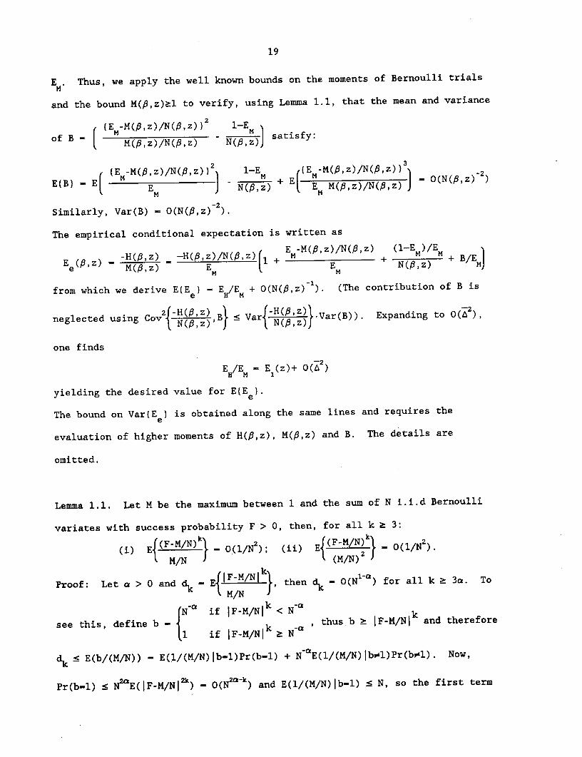
E . Thus, we apply the well known bounds on the moments of Bernoulli trialsM
and the bound M(P,z)>l to verify, using Lemma 1.1, that the mean and variance
( (E -M(,z)/N(,z)) 1-EM
of B- M(M,z)/N(f,z) N(,z) satis
B (E -M(-f,z)/N(,z))2 1-E {E -M(f,z)/N(f,z))
2 ME(B) - Et( M EM - )----Z- ( E[ O(N(Pz )
Similarly, Var(B) - O(N(P,z)2).
The empirical conditional expectation is written as
, -H(f, z) -H(f,z)/N( +l,z) E 1 ( /E + B/E MEe M(3,z) E ( E N(+,z) H
-M
from which we derive E(E - E /E, + O(N(f,z) 1). (The contribution of B is
neglected using Cov ( -H(z )-H(, Var Z}. Var(B)). Expanding to 0(2),neglected using Cov N-f,z),B < VarN
one finds
EH/E M - E (z)+ 0(A 2)
yielding the desired value for E(E ).
The bound on Var(E ) is obtained along the same lines and requires the
evaluation of higher moments of H(f,z), M(3,z) and B. The details are
omitted.
Lemma 1.1. Let M be the maximum between 1 and the sum of N i.i.d Bernoulli
variates with success probability F > 0, then, for all k > 3:
(i) Et }- - o(1/N2); (ii) E{[( - 0(1/N%.
Proof: Let a > 0 and dk - E{ 'Nl }, then dk - 0(N1 a ) for all k > 3a. To
N a if IF-M/NI k< N k
see this, define b - , thus b > IF-M/N k and therefore
1- if |F-M/Nlk | N-
dk <N E(b/ (M/N)) - )E(l/(M/N)|b-l +) + N E/M/N)|bl)Pr(bs l ) . Now,
Pr(b-l) < N2aE(IF-M/Nl2k) - O(Nz2-k) and E(1/(M/N) b-l) - N, so the first term
20
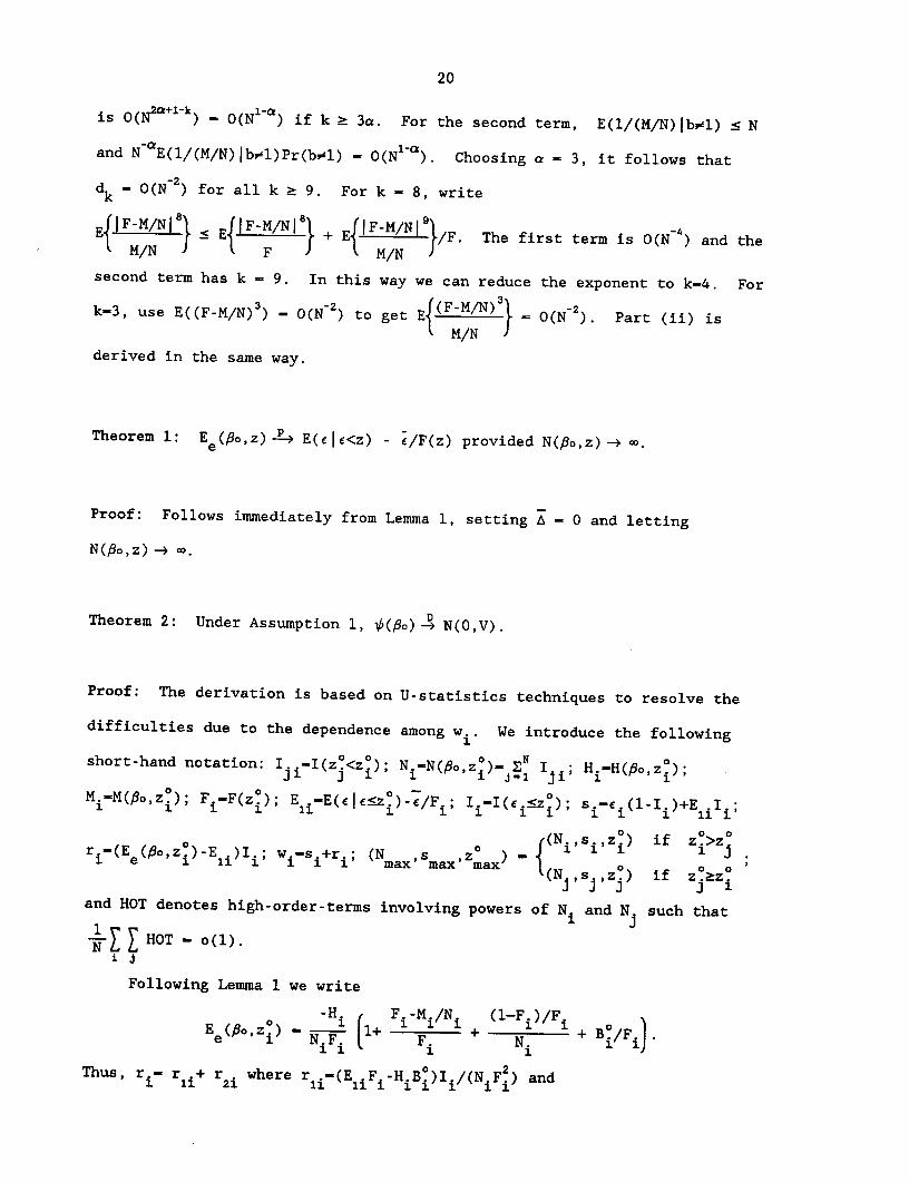
is O(N a +l ) - O(N 1') if k > 3a. For the second term, E(1/(M/N) |bl) < N
and N aE(l/(M/N) Ibl)Pr(bol) - O(N1-a). Choosing a - 3, it follows that
dk - O(N-2) for all k > 9. For k - 8, write
El EI - + E IF/N + M/ I /F. The first term is O(N- ) and theM/N F ' M/N
second term has k - 9. In this way we can reduce the exponent to k-4. For
k-3, use E((F-M/N)3) - O(N-2) to get E (FM/ O(N ). Part (ii) isM/N 3
derived in the same way.
Theorem 1: E (Po,z) - E(cee<z) - e/F(z) provided N(Po,z)- co.
Proof: Follows immediately from Lemma 1, setting A - 0 and letting
N(B3o,z) - o.
Theorem 2: Under Assumption 1, b(Bo)-_ N(0,V).
Proof: The derivation is based on U-statistics techniques to resolve the
difficulties due to the dependence among w.. We introduce the following
short-hand notation: Iji-I(zj<zi); Ni-N(Bo,z')- j Ii; Hi-H(0o,zi);
M -M(Po,zi); F.-F(z ); E -E(e z)/ I-I( z); s-(1-Ii)+E I1 2 1 2 1 1 i ii
((N.szi) if z.>z.r0, - );,.0 i i - 13ri(Ee(P'Zi)-Ei)Ii Wi-si i; (Nmax'Smaxmax' ax 1 (Nsz) if zo
(Njsjj if zj iand HOT denotes high-order-terms involving powers of Ni and Nj such that
i jN- E EHOT - o(l).
Following Lemma 1 we write
-'Hi F-M/N (1-Fi)/Fi o )E(PoZ 0 ) - NH i (l+ + B/F i .
F where (E -N i
Thus, ri- rli+ ri where r .i-(EiFi-H B )Ii/(N F2 ) andi ii A 1~21 ii i i ii i

21
J -Hi 1- F -M i/Ni + Fi)/Fi1 I
2i - { N1 - - + NiF.J iN i .F. iiNi i 1
N
The term involving r i can be ignored, as [ xiri/V/N - 0 (cf. Lemma 1). The
1i-1 N
second term has been constructed to ensure that E(rzi)-0, thus [ xir2 //N hasi-l
the structure of U-statistics, albeit not in the standard symmetric form.
Indeed, a straightforward evaluation gives
i E( N X - XI +mi
where Smi - mI(em>Zi ) + EliI( mzi) and
msi - (m I(e >zi) + EliFi) + E iFi(I(emszi) - Fi) Notice that each iN
depends only on e and hence is independent of TNm for all m'# m. Thus
N N
TN - 'rNm is a convenient approximation to T xiri//N. Obviously, E(TN)-O.M-mS~~~~~~ ~ ~ii
Furthermore, E(s s) Var(s ), E(s' ) 0(1), E(s' .s') - 0(1) andm Mj m Smax) E(Ssmi ) O(1) E(Sij) O(1) andm m
Var( N) E xxI I m Var(s a)/(N.N) + HOT. Since~Nm Nij jmi mj max J
II - I(z < min(zi,zj°), the summation over m is easily carried out:mi mj m JJ
Var(TN) - Var(INm) N L X xix Var(smax)/Nmaxm i j
Following Lemma 1, we find E(ri) - 0 and Cov(r2i,rzj) - Var(smax)/Nmax + HOT,
rso t Varxr2 / E Ai (smax max (')i- i j
(E xr 2i/N - i2 Var E xir i//N Var(N) - o(l) (cf. Lehmann, 1975,
pp. 362-363). Thus, E xiri/N - ) - 0.i-1
Having observed that the term with si' has a negligible contribution, we
(-··- ·· XiImi /adobtainconsider the quantities Nm- xmsm - s /N and obtain
(+(Bo) - wNm) -] °0. The moments of wN are evaluated in the same way
as those of TNm: E(wNm) - andas those of ~Nm: E(wNm) - 0 and
22
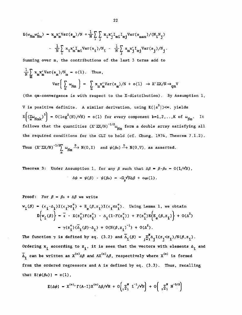
E(w*W (<-) x x'V Var(sm)/N + x.x:I I .1 .Var(s )/(NiN j.)
-±~i j
( Nm Nm Xm r(m)/ N I j Ximlmj max
N Viar(s,)/Ni xN x.m I jVar(s )/N
Summing over m, the contributions of the last 3 terms add to
x xmx'Var(sm)/N - o(l). Thus,mLm m m)
m
Var( Nm ) - x'Var(s )/N + o(l) -> X'ZX/N-4 V
(the qm-convergence is with respect to the X-distribution). By Assumption 1,
V is positive definite. A similar derivation, using E(Is 3 |)<., yields
E((SwNmk)) - O(log (N)//N) - o(l) for every component k-l,2,..,K of uNm. It
follows that the quantities (X'ZX/N) w/ form a double array satisfying all
the required conditions for the CLT to hold (cf. Chung, 1974, Theorem 7.1.2).
Thus (X'ZX/N) 1/2 WN -m- N(0,I) and V(fo) -- N(0,V), as asserted.m
Theorem 3: Under Assumption 1, for any P such that AP p- P-o - 0(1//N),
AV, - (S) - () o) = -() - /NAB + oqm(l).N
Proof: For P - Po + AP we write
wi(P) - (ei-Ai)I(fi>zi) + Ee(P,zi)I(i <zi). Using Lemma 1, we obtain
E{wi()} - - E(zi)F(z i ) - A(l-F(zi)) + F(z?)EEe(),z i ) + (A )
- 7(zi)(Ai()-Ai) + O(N(P,zi) -) + 0(A2).
The function 7 is defined by eq. (3.2) and Ai(P) - ENAjI(zj<zi)/N(,z i).
Ordering xi according to zi, it is seen that the vectors with elements Ai and
Ai can be written as X(° A and AX( AP, respectively where X (° ) is formed
from the ordered regressors and A is defined by eq. (3.3). Thus, recalling
that Et((So)) - o(l),
E(A) - X(o)'r(A-I)X(o)Ai// o(N + O[ i-1/N + o[ N N-3/2)

23
- -nVNAB + o(l).
This result is not yet quite what is needed, since the ordering is
carried out according to zi rather than zi, leaving n dependent on P. To1 1 N
remedy for this we show in Lemma 2 that Ai(P) - Ai(fo) - O(N(fio,zi) ). It
follows that the additional term introduced by evaluating 0 at Po is also ofN
o(l). The more tedious evaluation of Var({A) is carried out in the same way
as the derivation of Var((p8o)) in the proof of Theorem 2. One notes that the
leading terms are proportional to A8 and therefore Var({A) - o(l) although
both Var({(po)) and Var(o(f)) are of 0(1).
Lemma 2: Under Assumption 1
(i) ExN(9,zi) - N(o,z')} - O(Nl||A||).
(ii) Ex{N(o,zi ) A (P) - A(fio)) - O(NIA 112 ).
In particular, for AP - O(1//N), E zN(Boi,z i)(-) - Ai(Po)) = 0(1).
Proof: N(9,zi)-N(8o,zi) - I(zj<zi) - I(z°<z) - I(z-A<z- ) - I(z<z).
i Ji i i
Let e - 2-Sup||x|||A4| - 0(A8), then IN(P,zi) - N(<o,zi)l I(|Iz-zil<e).x i
jsi
For a given zo, (i) follows immediately from Assumption l-(iii). Furthermore,
Ai(I(z <zi) - I(z<zi)) - N(P,z ) - N(o,z)A (P) - A (Po) - ) A (P) - 1
i 1 N(Po,z ) N(Po,zi)O Ojoi
or N(po,z)lAi(9P) - -A i(o) < 2e E I(|zj-z|l<e) and (ii) is derived in the
jfi
same way as (i). Corresponding bounds can be deduced for the variances.
The proof of Theorem 4 utilizes:
Lemma 3: Under assumption 2, for all C in the domain of Fz
(i) E fik IC - ) - 0 for k>l and all i.ik iK i'*'

24
(ii) Elk jk I il- - 0 for k> or k'>l and i'j.
(iii) E ~(O)0(() (0) Ekkik(ii) jo mk"'o) (o) - 0 for k>l and ij i1l i'm, or k'>l and j'i
j'l jAm, or k">l and l4i l^j lrm, or k"'>l and m'i mij mol.
Remark: It follows that the corresponding unconditional expectations also
vanish, so that except for k-l, fik mimic the properties of the unorderedik
fik-
Proof: Denote by p(fil) the index of fil after ordering, indicating that
p(ril)-l elements of the first column of Z are smaller than il while N-p( il)N
elements are larger. Thus fik) ' jk I((jl)-i) . Taking expectation, we
obtain
^ik 'il - ZJ j-E (klP(~jl)i;fjl-[)Prb(p(fl)-iri'i) '
i-h k fProb l (( )-ls conit o)l
The last step follows since given rjl-S' P(<jl)-i entails conditions on ml
for moj only and hence is independent of Sjk- The resulting sum vanishes
identically because E(ijk jl--T 0 according to Assumption 2(ii). Thus, (i)
is established. Parts (ii) and (iii) are derived following the same reasoning,
utilizing the factorization property
E kfmk'jl - ml-") - E(jkIjl -) Emk' |m 1-"
Theorem 4: Under Assumptions 1-3:
(i) nN converges in quadratic mean to a nonsingular limit 0;
(ii) 0 - po + 0-1 (o)//N is a /N-consistent solution to the FPE.
Proof: We recall that (i) is equivalent to the proposition that
Z' (r)(I-A)Z( )/N has a nonsingular limit. Ordering plays no role in the

25
evaluation of Z' (Frz')/N, so the definition of Z implies Z' (O)FZ' /N - I,
and only Z' ()rAZ()/N requires further consideration. We begin by showing
that (Z' ()rAZ /N)mk- 0 unless m-k-l. For j>2 let Rjk - fik (-1)I ~n - Jmk qm j ik
jr)mk - jm jl Jk^ w ^/i -
and ('o)-y(CN)-m l)R Lemma 3 implies that-
(where f is the density function of %l))' andji=
N () (o) (lo) (( _o) (o)Var1 E L* -Y(Co.jl )Rjk /NJ 0 if kol or mr'l. Thus, only rAZ I/Nj 1
survives. To evaluate this element we write it in terms of the unordered
N f s il i jIi N. >0
regressors as E Sjl-(CoSjl)Rj/N, where Rjl 1 il i j
j-i j if N.- 0
Ejm 7(C°Sl )Rji) - j(C°)E(R|ji j -- )fz()d1. It is convenient to treat
differently the cases where F (r) is large or small, i.e., for some e>O, let
-F w (e) and consider first > . As in the derivation of Lemma 1, we write
il I( i< jl)/NIN NIN - F (/l)N
jl Fz( j) N/N
N /N - F Z )andand verify that E -Fjl) -) and
N Nj/Nl J
Var| N;/N 1 i jl - (l/(NF()). Thus,
N./N J z
E(R sjl- ) - E(0f + o(l/(NF(0))). F or m<. we use the fact that Rl is
bounded to obtain j-(Co()E(R jlleI-f f z() d - 0(e). Finally, by choosing
min
e such that e - 0 and Ne - wo we get
E([j 1s(Cor)Ri) -+ fjT(CO)E()R )fz()d . A similar derivation gives

26
VarRjl E(fjl)) -4 0. It follows that
(Z'¢(rAZO)/N) 1 1 - fjl7(Co jl)Ez(fl )/N -4 0. The sum on the lhs'
consists of independent terms, each with the mean ffY(Cof)Ez ()fz(f)df. Thus
(Z' WFAZ() /N)1 -qm ff(CO)EZ(f)f )d.
In fact, the same reasoning can be used to show that
(Z'(o)rz()/N) 1 1 q fS27(CoO)fz(f)dr - 1.
Summarizing, all the elements of Z' ()r(I-A)Z()/N converge to the
corresponding elements of I except for the 1,1 element, whose limit equals
8 - f f 7(Co)[.r-Ez(f)jfz()dy, which establishes (i). Let 0 denote the
probability limit of N and define p - Po + n-1'(Po)//N. According to theorem
2, (qo) - 0(1), and the nonsingularity of 0 implies that VN(-fBo) is also
A% AO (1). Thus, we can use Theorem 3 to obtain b(pf) - (fo)- VNN(6-6o) +
o (1) - ob(P) - Q/N($-$o) + o (1) - o (1), implying that $ is aqm qm qm
/N-consistent solution to the FPE.
Theorem 5: Let ({mm)1. .M be the set of distinct (to 0(1//N)) solutions ofA ethe FPE. Then, under assumptions 1-4, P - argmin Qe(P ) is a v'N-consistent
m-l..Mestimator of Bo.
Proof: We first show that for every P E S$, Qe()-( q .le, QN P) QN(P)--qm O.
Qe () - Q0() - ((y+z) I(y1>O) - (E (z)-2E (z)A +^)F (zF ) / N
»-1
+ 2, IEN (fi,) [(Ec(z)-A) C (I(yi>o N
N + ^ I(y,>0) (EZ i iz i )- i+Zi) >0 / N
I i I ec C i~~~~~~~
27
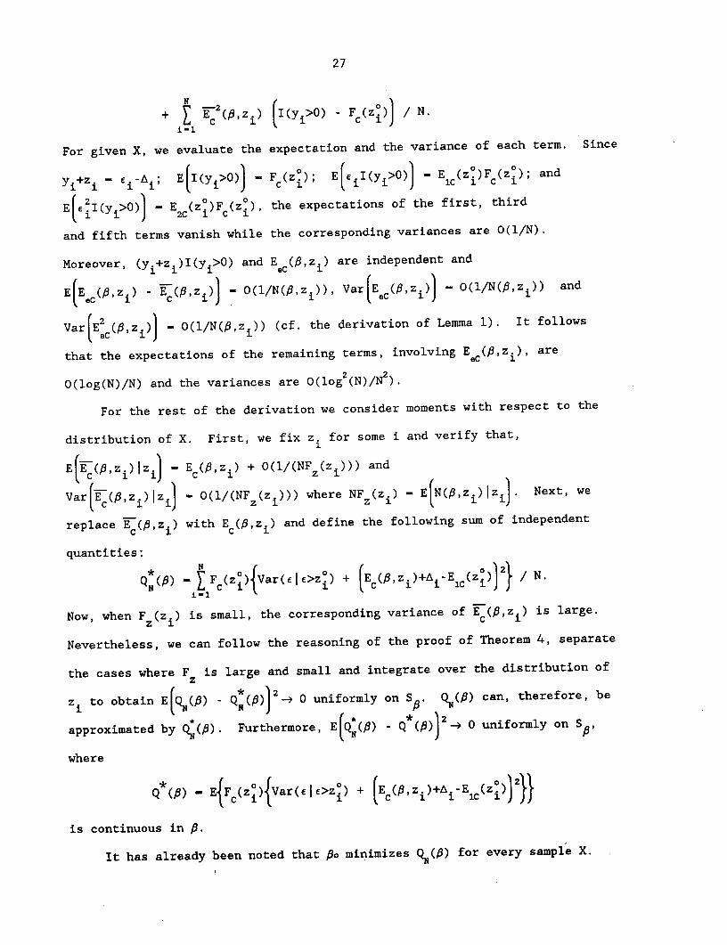
+ e i) (I(i>O) - Fc(Z)) / N.
For given X, we evaluate the expectation and the variance of each term. Since
i - e -A EI(yI>O) F- cF(z); E( iI(yi>O)) E (zo)Fc(zo); and
E2eI(Yi>)) - Ec (zZ)F (zi), the expectations of the first, thirdI 1 1 J 2C i C 1
and fifth terms vanish while the corresponding variances are 0(1/N).
Moreover, (yi+z,)I(yi>0) and Ec (f,zi) are independent and
E E 0(az) - E(P,z))- O(/N(P,zi)), Var(EC ( (1/N(,z)) and
Var(E2c(pz)) - 0(l/N(P,z.)) (cf. the derivation of Lemma 1). It follows
that the expectations of the remaining terms, involving E c(',zi), are
O(log(N)/N) and the variances are O(log (N)/N2).
For the rest of the derivation we consider moments with respect to the
distribution of X. First, we fix z. for some i and verify that,
E((i,z)Iz i) Ec(',zi) + 0(l/(NF (z.))) and
Varf(r ,z)zl - 0(l/(NF (zi))) where NFZ(Zi) - EfN(.zi) Iz . Next, we
replace Ec(,z i) with Ec(9,zi) and define the following sum of independent
quantities:
Q (8) - Fc(Z'){Var(ele>zt) + (Ec(,zi)+Ai Elc(Z ) / N.
Now, when F (zi) is small, the corresponding variance of Ec(,z i) is large.
Nevertheless, we can follow the reasoning of the proof of Theorem 4, separate
the cases where F is large and small and integrate over the distribution ofz
zi to obtain E(QN(P) - QN(8))2 0 uniformly on S . QN() can, therefore, be
approximated by Q(A). Furthermore, E (QN() - Q*(P))2 0 uniformly on S ,
where
Q (P) - E {F(z){Var(eIe>Zo) + (E (,zi)+Ai Elc(Z))2}}
is continuous in A.
It has already been noted that 6o minimizes QN(3) for every sample X.
28
Thus, it must also minimize Q (6). In fact, the identification condition
4(iii) ensures that So is the unique minimizer. Calculated at the consistent
root of the FPE, QNe() converges (in quadratic mean) to the global minimum
Q (po), whereas, by virtue of the identification condition and the continuity
* eof Q (P), at any other root the corresponding value of QN is kept well above
N~e
this minimum. It follows that the choice of the root that minimizes Q (P)
provides a consistent estimator.
A
Theorem 6: Under Assumptions 1-3, VN(P - Bo) N(O,'OVI' ).
Proof: Given in the text.

29
References
Breiman, L., Y. Tsur and A. Zemel (1989): "A Simple Estimator for
Censored Regression Models with Known Error Distribution", Technical
Report No. 198, Dept. of Statistics, University of California, Berkeley.
Buckley, J. and I. James (1979): "Linear Regression with Censored Data",
Biometrica, 66, 429-436.
Chung, K. L. (1974): "A Course in Probability Theory, 2nd ed. Academic Press,
New York.
Dempster, A. P., N. M. Laird and D. B. Rubin (1977): "Maximum Likelihood
from Incomplete Data via the EM Algorithm", Journal of the Royal
Statistical Society, Series B, 39, 1-22.
Duncan, G. M. (1986): "A Robust Censored Regression Estimator", Journal of
Econometrics, 32, 5-34.
Fernandez, L. (1986): "Non-parametric Maximum Likelihood Estimation of
Censored Regression Models", Journal of Econometrics, 32, 35-57.
Horowitz, J. L. (1986): "A Distribution-Free Least Squares Estimator for
Censored Linear Regression Models", Journal of Econometrics, 32, 59-84.
James, I. R. and P. J. Smith (1984): "Consistency Results for Linear
Regression with Censored Data", Ann. Statist., 12, 590-600.
Lee, L.-F. (1988): "A Semiparametric Nonlinear Least Square Estimator of
Truncated Regression Models", Dept. of Economics, University of
Minnesota.
Lehmann, E. L. (1975): "Nonparametrics: Statistical Methods Based on Ranks",
Holden-Day, San Francisco.
Nawata, K. (1990): "Robust Estimation Based on Grouped-Adjusted Data in
Censored Regression Models," Journal of Econometrics, 43, 337-362.
Powell, J. L. (1986): "Symmetrically Trimmed Least Squares Estimation for
Tobit Models", Econometrica, 54, 1435-1460.
Powell, J. L. (1984): "Least Absolute Deviations Estimation for Censored
Regression Model", Journal of Econometrics, 25, 303-325.
Ritov, Y. (1990): "Estimation in a Linear Regression Model with Censored
Data", Ann. Statist., 18, 303-328.
Ritov, Y. and M. Fygenson (1990): "A Monotone Estimating Equation for Censored
Regression," Dept. of Statistics, The Hebrew University of Jerusalem.
Tsiatis, A. A. (1990): "Estimating Regression Parameters Using Linear Rank
Tests for Censored Data", Ann. Statist., 18, 354-372.
Tsur, Y. (1983): "On Efficient Estimation of Some Limited Dependent Variable
Models", Dept. of Agricultural & Resource Economics, Giannini
Foundation Working Paper 281, University of California, Berkeley.