STABLITY PROPERTIES OF A FIELD-REVERSED

ION LAYER IN A BACKGUND PIASMA

by

Han S. Uhm and Ronald C. Davidson

PFC/JA-78-7

Suhmitted to Physics of Fluids, August 1978

STABILITY PROPERTIES OF A FIELD-REVERSED ION LAYER IN A BACKGROUND PLASMA

Han S.' Uhm and. Ronald C. DavidsonPlasma Fusion Center

Massachusetts Institute of TechnologyCambridge, Massachusetts 02139

ABSTRACT

Stability properties of an intense proton layer (P-layer) immersed

in a background plasma are investigated within the framework of a hybrid

model in which the layer ions are described by the Vlasov equation, and

the background plasma electrons and ions are described as macroscopic,

cold fluids. Moreover, the stability analysis is carried out for

frequencies near multiples of the mean rotational frequency of the layer.

It is assumed that the layer is thin, with radial thickness (2a) much

smaller than the mean radius (R0 ). Electromagnetic stability properties

are calculated for flute perturbations (D/9z=O) about a P-layer with

rectangular density profile, described by the rigid-rotor equilibrium

0distribution function f b=(mnb/2-r)d(U-)G(vz), where nb and T are

constants, mi is the mass of the layer ions, G(v z) is the parallel

velocity distribution, and U is an effective perpendicular energy

variable. Stability properties are investigated including the effects

of (a) the equilibrium magnetic field depression produced by the P-layer,

(b) transverse magnetic perturbations (,B#O), (c) small (but finite)

transverse temperature of the layer ions, and (d) the dielectric

properties of the background plasma. All of these effects are shown to

have an important influence on stability behavior. For example,

for a dense background plasma, the system can be easily stabilized by

a sufficiently large transverse temperature of the layer ions.

*Permanert address: Nuclear Branch, Naval Surface Weapons Center. SilverSpring, Md. 20910

2

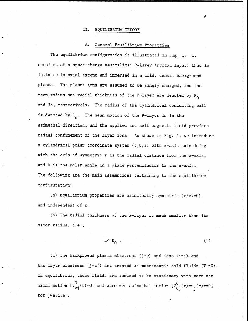
I. INTRODUCTION

Field-reversed ion layers and rings have received considerable

recent attention as magnetic confinement configurations'for fusion

plasmas.1-8 Such layers and rings are likely subject to various

macro- and microinstabilities.9-13 For example, recent theoretical

studies of the negative-massl1-13 stability properties of a weakly

diamagnetic ion layer embedded in a background plasma predict instability1 3

for perturbations with frequency near harmonics of the layer rotational

13frequency. These studies have been carried out for a low-intensity

ion layer characterized by v<<l, where v=Nbbe 2/m c2 is Budker's parameter

for the layer ions, and Nb=27r c dr r n (r) is the number of ions

per unit axial length. A more general stability analysis is required

to investigate stability properties for an intense field-reversed

ion layer characterized by v>>l.

This paper develops a hybrid theory of the negative-mass instability

for intense ion layers with arbitrary degree of field reversal. The

present work extends the previous self-consistent theory13 of the

negative-mass instability developed for v<<l. The analysis is carried

out within the framework of a hybrid (Vlasov-fluid) model in which

the layer electrons and background plasma electrons and ions are

described as macroscopic, cold fluids immersed in an axial magnetic

0field Bz (r)z, and the layer ions are described by the Vlasov equation.

We assume that the layer is thin [Eq. (1)], i.e., the radial thickness

(2a) of the layer is small in comparison with the mean radius R '

Equilibrium and stability properties are calculated for the specific

choice of ion layer distribution function [Eq. (2)]

f 0 (H- Pa, v ) = 6(U-T)G(v)b 8 z 27 z

3

where nb, W9, T are constants, G(v z) is the parallel velocity

distribution, HI is the perpendicular energy, P, is the canonical

angular momentum, and U is the effective energy variable defined in

Eq. (3).

One of the important features of the equilibrium analysis

(Sec. II) is that the equilibrium distribution function in Eq. (2)

corresponds to a sharp-boundary density profile [Eq. (9)], with uniform

angular velocity profile over the layer cross section [Eq. (12)],

and nonzero transverse temperature [Eq. (13)]. Moreover,

defining the magnetic compression ratio n by n=B (r=R )/B [Eq. (16)],

0where B (r=R1 ) and B0 are the axial magnetic fields at the inner and

outer surfaces of the layer, we find [Eq. (26)]

v=(l-n) / (+n) ,

for a thin layer with a<<R Because v>O, it is important to note from

Eq. (26) that the allowable range of compression ratio is given by -l<ri<l.

Moreover, in order to produce a sizeable field depression, a relatively

large value of Budker's parameter (v2l) is required. We also emphasize

that the rigid-rotor distribution function in Eq. (2) has an associated

spread in canonical angular momentum (A) [Eq. (32)], which plays an

important role in determining stability behavior.11

The electromagnetic stability analysis in Secs. III-V includes the

effects of (a) the equilibrium magnetic field depression produced

by the P-layer, (b) transverse magnetic perturbations (BO0), (c) small

(but finite) transverse temperature of the layer ions, and (d) the

dielectric properties of the background plasma. The analysis is carried

out within the framework of the linearized Vlasov-fluid and Maxwell

equations, assuming that all perturbed quantities are independent of

4

axial coordinate <3/3z=0). Moreover, the stability properties are

investigated for eigenfrequency near multiples of the mean P-layer

rotational frequency, i.e., W-Zo-6<<W r, where w is the complex eigen-

frequency, Z is the azimuthal harmonic number, w is the mean rotational

frequency of the P-layer, and w r is the radial betatron frequency of the

layer ions. It is also assumed that the background plasma has a step-

function density profile (Fig. 5).

The formal stability analysis for perturbations with a/az=O

is carried out in Secs. III and IV. The perturbed charge density

of the layer ions is calculated in Sec. III, including kinetic ion

orbit effects. A fully electromagnetic eigenvalue equation is obtained

in Sec. IV, including the dielectric properties of the background

plasma. Equation (69), when combined with Eq. (68), constitute one of the

main results of this paper and can be used to investigate stability proper-

ties for a broad range of system parameters. In this regard, we emphasize

that Eq. (69) has been derived with no a priori restriction on the back-

ground plasma density.

In Sec. V, a detailed analytic investigation of

electromagnetic stability properties is carried out for a

dense plasma background. For certain ranges of system parameters,

it is found that the system is unstable. Moreover, the instability

11-13mechanism is similar to that for the negative-mass instability,

including the effects of transverse temperature of the layer ions,

and the dielectric properties of the background plasma. For

example, in the case where the plasma density outside the layer is equal

to zero (a=O), the approximate dispersion relation is given by (Eq. (90)]

5a

23 + 22 ZA + 2, 2-n - 0+C 2 Y(l+n) 2

where Q is the normalized Doppler-shifted eigenfrequency defined in Eq.

(88), and the parameters C and X are defined in Eqs. (87) and (91),

respectively. In Eq. (90), c' [Eq. (87)] is an oscillatory function

of plasma density. However, the value of C', averaged over each period,

is an increasing function of plasma density. We therefore conclude

from Eq. (90) that the system is completely stabilized if the plasma density

is sufficiently high. The terms proportional to ZA in Eq. (90) also have

a stabilizing influence, thereby quenching the growth rate for sufficiently

high Z values. This effect is most pronounced when the magnetic

compression ratio n is close to zero. A similar stabilization for high Z

values has also been demonstrated for intense relativistic E-layers. 11

A numerical investigation of stability properties is carried out

in Sec. V.C for general values of an (the plasma density outside thep

layer). Several points are noteworthy in this regard. First, the

instability growth rate is greatly reduced as n-*O. This feature is evident

from Eq. (90) for a=0. Second, stability properties are almost independent

of a, provided a is sufficiently small (a<0.5, say). Finally, in

parameter regimes where instability does exist, the maximum growth

rate can be a substantial fraction of ion cyclotron frequency w Ci'

In Sec. VI, a numerical investigation of stability properties is

carried out for an arbitrary value of background plasma density, assuming

a rectangular density profile with a = 0. The eigenfunction (r) is

obtained numerically from the eigenvalue equation (72). It is found from

the numerical analysis that the electrostatic eigenfunction $(r)=(r/R)

5b

is a very good approximation to the actual eigenfunction for a field-

reversed ion layer in a low-density background plasma satisfying

pi. /c < 1, where w . is the background ion plasma frequency and c is

the speed of light invacuo. However, the electromagnetic effects

associated with the background plasma dielectric response become dominant

when the plasma density is sufficiently high that w R /c Z 2. Generally

speaking, the numerical investigation of stability properties in Sec. VI

gives similar results to those obtained analytically in Sec. V.

6

II. EQUILIBRIUM THEORY

A. General Equilibrium Properties

The equilibrium configuration is illustrated in Fig. 1. It

consists of a space-charge neutralized P-layer (proton layer) that is

infinite in axial extent and immersed in a cold, dense, background

plasma. The plasma ions are assumed to be singly charged, and the

mean radius and radial thickness of the P-layer are denoted by R0

and 2a, respectively. The radius of the cylindrical conducting wall

is denoted by R C. The mean motion of the P-layer is in the

azimuthal direction, and the applied and self magnetic field provides

radial confinement of the layer ions. As shown in Fig. 1, we introduce

a cylindrical polar coordinate system (r,e,z) with z-axis coinciding

with the axis of symmetry; r is the radial distance from the z-axis,

and 6 is the polar angle in a plane perpendicular to the z-axis.

The following are the main assumptions pertaining to the equilibrium

configuration:

(a) Equilibrium properties are azimuthally symmetric (3/0O)

and independent of z.

(b) The radial thickness of the P-layer is much smaller than its

major radius, i.e.,

a<<R

((c) The background plasma electrons (j=e) and ions (j=i), and

the layer electrons (j=e') are treated as macroscopic cold fluids (T =O).

In equilibrium, these fluids are assumed to be stationary with zero net

0 0axial motion [V .(r)=01 and zero net azimuthal motion [V 0 (r)=w.(r)r=0]zJ 8 ]

for j=e,i,e'.

7

(d) The background plasma equilibrium is assumed. to be electrically

a aneutral with n (r)=n (r). In addition, the equilibrium charge densitySe

of the layer ions (j=b) is neutralized by the layer electrons (j=e')

with n 0(r)=n (r), and the equilibrium radial electric field is

0equal to zero, E (r)=O.

r

For- the layer ions, any distribution function f 0(;,) that is a

function of the single-particle constants of the motion in the

equilibrium fields is a solution to the steady-state (9/3t=0) Vlasov

equation. For present purposes, we consider the class of rigid-rotor

Vlasov equilibria described by4

fb0(H.L-W PO , )z 2-= M' (U-i')G(v) ,(2)

where nb' w0 , and T are constants, G(v z) is the parallel velocity

distribution with normalization dvzG(vz)=l, and the effective energy

variable U is defined by

U=Hj -.o e +MiR 2 /2+(e/c)Ro WA 0) ( (3)

In Eq. (3), Hi, is the perpendicular energy

2 2H =(M /2) (v 2+V ) (4)

and P 6 is the canonical angular momentum

0Pe =r[m.v +(e/c)A0 (r)]

Here e and m are the proton charge and mass, respectively, c is the

speed of light in vacuo, and vr and v are the radial and axial velocities

of a layer ion. The e-component of the equilibrium vector potential,

A0(r), is to be calculated self-consistently from the steady-statea~)

8

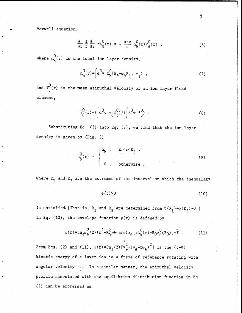
Maxwell equation,

9 1 ; rA (r) = - n (r)V (r) , (6)

where n (r) is the local ion layer density,

b b3 aan(r)= dv fb(H - Pe' v)(7

0and V (r) is the mean azimuthal velocity of an ion layer fluid

element,

VO(r)=( d 3v v6 f )/({d3v f (8)

Substituting Eq. (2) into Eq. (7), we find that the ion layer

density is given by (Fig. 2)

n b , R <r<R2

nb(r) (0 , otherwise

where R and R. are the extremes of the interval on which the inequality

(r)>0 (10)

is satisfied. [That is, R and R2 are determined from (R1 )=(R 2)=O-1

In Eq. (10), the envelope function *(r) is defined by

2 2_2 0 06(r)=(m w /2)(-R 0 )+(e/c)w a [rA (r)-ROA (Ro)]+T

From Eqs. (2) and (11), $(r)=(m /2)[v +(v -rwa) ] is the (r-6)

kinetic energy of a layer ion in a frame of reference rotating with

angular velocity w . In a similar manner, the azimuthal velocity

profile associated with the equilibrium distribution function in Eq.

(.2) can be expressed as

9

0 (r)=rw, R <r<R (12)ver)w 1 2 (2

Equation (12) corresponds to a rigid-rotor angular velocity profile

over the layer cross section. Defining the effective temperature

0T,(r) for the transverse motion of the layer ions by

n (r) T,(r) =T d b v+v m

we find from Eqs. (2) and (11) that the transverse temperature profile

can be expressed as

T0(r) =(r) R <r<R (13)11 2

Evidently, the envelope function $(r)>0 defined in Eq. (11) is

identical to the transverse temperature profile.

We note from Eq. (9) that the density profile has sharp radial

boundaries at R and R Substituting Eq. (12) into Eq. (6). we

find that the equilibrium axial magnetic field within the P-layer

(R1<r<R 2) can be expressed as

0 2 2B (r)B +(27re/c)wenb(R 2-r ) (14)z~ 02

where B0 is the axial magnetic field at r>R 2. The corresponding

0equilibrium vector potential A (r) is given bya

90 0 22A 0r=O e(Ro)+(Bo/2)(r2-R0 )

(15)

+(7e/2c)wgnb 2_R 2)[2R 2_(r 2+R )2

For notational convenience in the subsequent analysis, we introduce

the magnetic compression ratio n defined by

10

0rn=B (r=R )/B' (16)z 1 0

which characterizes the change in axial magnetic field. We further

introduce Budker's parameter for the layer ions

R

=21r(e2/m c 2) dr r n (r) . (17)

Substituting Eq. (14) into Eq. (16) and making use of Eq. (17)

gives

we/i.(T--l) /2V , (18)Sci

where wci=eB0/ i/c is the ion cyclotron frequency at r=R 2 '

The axial magnetic field profile is illustrated in Fig. 3.

Equations (11) and (15) completely determine the functional form

of the envelope function $(r). We note from Eq. (15) that equilibrium

layer density (the term proportional to nb) can generally have a large

nonlinear influence on the location of the radial boundaries R and

R?. A sketch of $(r) versus r is illustrated in Fig. 4. Thus far,

R has been introduced in the analysis as an unspecified constant

parameter in Eq. (3). Without loss of generality, we choose R0

to correspond to that radius where $(r) passes through a maximum

in the interval R <r<R2 (Fig. 4),

h (r) JrR0 . (19)

Substituting Eq. (11) into Eq. (19) we find

w +(e/m.c)B (R )=O (20)9 i z 0

where use has been made of Eqs. (14) and (15).

11

Equation (20) is simply a statement of radial force balance on an

ion layer fluid element at r=R . Further general equilibrium properties

associated with the distribution function in Eq. (2) are discussed in

Ref. 4.

B. Thin-Layer Approximation with a/R «<

We now specialize to the case of a thin layer with (R2-R )/R 0<<,

and Taylor-expand Eq. (11) about r=RO,

1 2 2(r)=T - m wr (r-R0 ) + ... (21)

where

2 e-= R - B (r) = 2 6 .- (22)r m r2 M.. 0 3r z R b 0

Sr=RHere, wr can be identified with the betatron frequency for radial

oscillations about the equilibrium radius R In Eq. (22), w247e 2n/M

is the plasma frequency-squared for the layer ions, and 2 0R 22 /C

Defining the half-thickness of the layer by

1/2 (3a(2T/m )/W r (23)

we readily determine R1=R -a and R 2=R 0+a from X(r)=0 and Eq. (21).

It is also noteworthy from Eq. (22) that the betatron frequency

wr is directly proportional to w0 for the rigid-rotor equilibrium

described by Eq. (2). This is considerably different from the

result obtained in Ref. 12 for the choice of distribution function

in which all of the layer ions have the same values of canonical

angular momentum and the same value of energy.

For a thin P-layer, it is straightforward to show

S(r) = - I 4(r) (24)r=R 1rR2

12

from Eq. (21). Substituting Eq. (11) into Eq. (24) and making use

of definition in Eq. (16) gives

w/ .=-(1+n)/2 (25)

which determines the rotational frequency w in terms of the compression

ratio n. Moreover, substituting Eq. (25) into Eq. (18), we find

v=(1-n) /(l+n) . (26)

Equation (26) is one of the most important equilibrium results

pertaining to the choice of distribution function in Eq. (2), and

several points are noteworthy. First, Budker's parameter v for the

layer ions can be expressed exclusively in terms of the magnetic

field compression ratio n. Second, since v>O, the allowed range of

'n is given by

-J< J<1 (27)

Moreover, Budker's parameter rapidly increases to infinity as the

compression ratio approaches minus unity (ri+-l). In this regard,

strictly speaking, it is not possible to achieve complete field

reversal (n=-l) for the choice of distribution function in Eq. (2).

We note that v=l corresponds to zero compression ratio (n=O). Therefore,

in order to produce a significant field depression, we conclude

that a layer with a reasonably high value of Budker's parameter (v>l)

is necessary.

Of considerable interest for experimental application is the

relationship between the applied axial magnetic field B before injection

of the layer, and the external magnetic field B after injection. In

this regard, we assume that the magnetic flux inside the cylindrical

13

conductor is conser4ed, i.e.,

Rc

27 rdr B0 (r)=iTR B . (28)J0 z c

For a thin layer, the axial magnetic field profile can be approximated

by

0 ,O<r<R0

B (r) = Bz 0

1 , Ro<r<R,

and it is straightforward to show from Eq. (28) that

2B/B0 =1-(1-n)(R 0 /R ) . (29)0 0 c

For B/B0>0, we conclude from Eq. (29) that the magnetic compression ratio

is restricted to

2n<(Rc/R0 -1 (30)

Finally, we conclude this section by noting that the choice of

equilibrium distribution function in Eq. (2) yields a spread in

canonical angular momentum P . Defining the average canonical

angular momentum P0 as

2 0Po=M R 2W+(e/c)RoA0 (R)

it is straightforward to show from Eqs. (2) and (11) that

2 1/2P -PO iR 0 [2T/m -v (R0 21 (31)

where v r(R ) is the radial velocity of a layer ion at r=RO. For a

given transverse temperature ', those particles with v r(R0)=0 have

the maximum deviation in canonical angular momentum from the mean value

PO. Therefore, the maximum canonical angular momentum spread I can be

14

expressed as

A=IPe 8- = R0 (2m T) 1/2 (32)m

The parameter A defined in Eq. (32) plays an important role in

10determining the stability properties discussed in Secs. III and IV.

15

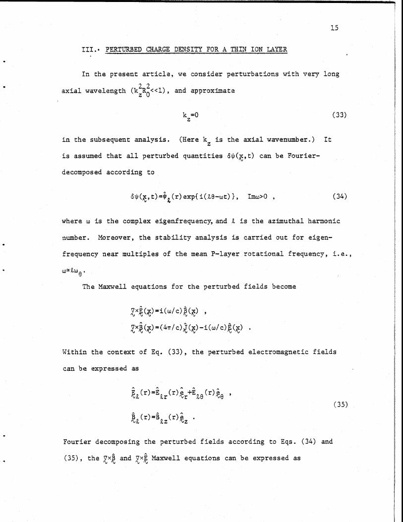
III.- PERTURBED CHARGE DENSITY FOR A THIN ION LAYER

In the present article, we consider perturbations with very long

axial wavelength (k R 1<<), and approximatezO0

k =0 (33)z

in the subsequent analysis. (Here kz is the axial wavenumber.) It

is assumed that all perturbed quantities Si( ,t) can be Fourier-

decomposed according to

*(g, t)=4Z (r)exp{ i(Z6-t)}, Imw>O , (34)

where w is the complex eigenfrequency, and t is the azimuthal harmonic

number. Moreover, the stability analysis is carried out for eigen-

frequency near multiples of the mean P-layer rotational frequency, i.e.,

The Maxwell equations for the perturbed fields become

x ( )=i(W/c)t(x),

VxB(x)=(41r/c)j(x)-i(w/c)E(x)

Within the context of Eq. (33), the perturbed electromagnetic fields

can be expressed as

E (r)=E (r)e +E (r),"QZ r nr Ze r e(35)

S(r)=9 (r)iz

Zz '\2z

Fourier decomposing the perturbed fields according to Eqs. (34) and

(35), the 7x$ and 7xE Maxwell equations can be expressed as

16

2 2 2 2 2 -1E Zr(r)=2, (W r /c -z ) (3/3r);

2 22 2 2 -1-47iro( r -Z c ) Jr)

(36)

B ()=Zw~w2 2 2 -1z (r)=-Zwr~~r /c-z c) (;/9r)p

+4rirZ(o2 r /c-z2 c) Jr (r)

where the function ^(r) is defined by

;(r)=ir ze(r)1 / (37)

and J r(r) is the perturbed radial current density.

After some straightforward algebra, the perturbed ion layer

11distribution function can be expressed as

0f r,v)=e b f dr exp{-i[wT-Z(6'-6)]}bZ NrJ au

(38)

+-Bvivx e(- ) ( + ' Zz) (Zr + iz/rJ

where r=t'-t. In obtaining Eq. (38), use has been made of 3U/3 v

m [vrr +(v-rt 0 )e 1, where e and are unit vectors in the r and e

directions, respectively. In Eq. (38), the trajectories, x'(t')

and v'(t') satisfy

V dt' % m.c% '%0'-dt v 0

where x'(t t =t)=x, and v'(t'=t)=v. The term E +v B /c in Eq. (38)V "I \J NJZr aGZz

can be further simplified. Making use of Eq. (36) we obtain

(r) + - B r)= - p (39)Zr Zc Zz a

Since the eigenfrequency of the perturbation is given approximately

by w=Zw,, Eq. (39) can be approximated by

17

EZr )+vB Zz(r)/c=-(3/3r)$(r) (40)

The evaluation of the orbit integral in Eq. (38) is generally

very complicated. However, for present purposes, we assume low-

frequency, long-wavelength perturbations characterized by

2 2

(41)

Za/R 0 <wr/ e'

where a is the half-thickness of the layer defined in Eq. (23).

Within the context of Eq. (41), it is valid for a thin layer to

approximate

(42)

*0'=6+[w8 +(v /R0 )cosalz7

where v± is the perpendicular speed in a frame of reference rotating

with angular velocity we. Moreover, v, is related to the effective

energy variable U by

U=(m /2) 2 [v+0 (r-R) 2 43)1 I r 0

with v --rwa=vcosa [see Eqs. (3), (11), and (21)]. Furthermore, the per.-

turbed ion layer distribution function can be simplified as [see Appendix A],

0ev, f 0

f bZ r,V)=iZ _ OCosa d_;x{-_r-( f6] . (44)

Substituting Eq. (42) into Eq. (44) gives

0ffb P(v /R)cosC

18

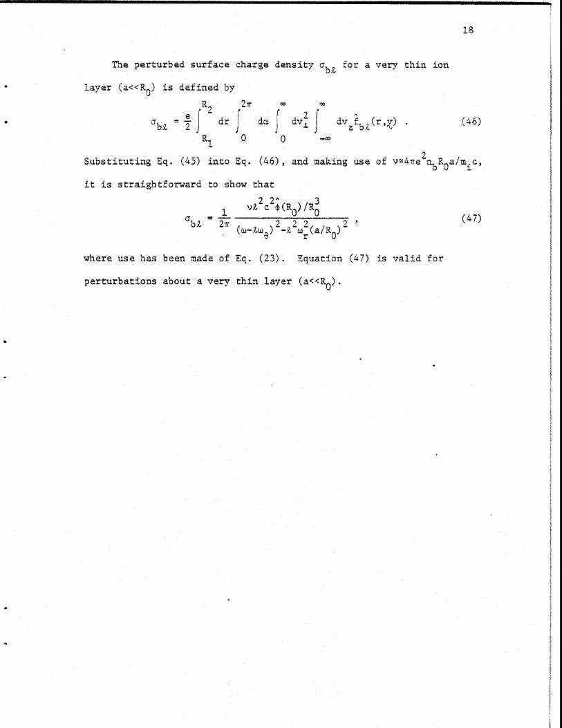
The perturbed surface charge density abZ for a very thin ion

layer (a<<R0 ) is defined by

R 2r

a = f dr da dv2f dv (rv) . (46)JZ - z bQ. "\1

R 0 0 -02.2

Substituting Eq. (45) into Eq. (46), and making use of v~47e 2nbR 0 a/m c,

it is straightforward to show that

2 2 31 vtc S(Obz 2 2 2

22 2'0 (47)abZ = r (w-z(e) 2 zr(a/R)2

where use has been made of Eq. (23). Equation (47) is valid for

perturbations about a very thin layer (a<<R ).

19

IV. ELECTROMAGNETIC STABILITY PROPETIES

A. General Eigenvalue Equation

As discussed at the beginning of Sec. II, the background plasma

components (j=e,i) and layer electrons (j=e') are treated as cold (T +O),

0 -macroscopic fluids immersed in an axial magnetic field Bz(r) z'

0where B (r) is approximated by

z

B (r)=B0 <r<R0 (48)z

R , R<r<Rc

for a thin layer. The momentum transfer equation and the continuity

equation for each cold-fluid component can be expressed as

+ V.- )V. = - + L),

(49)

(3/3t)n +7-(n.- )=O

where n ( ,t) is the density, V ( ,t) is the mean velocity, and e.

and m are charge and mass, respectively, of a particle of species j.

As illustrated in Fig. 5, the stability properties of the layer-

plasma system are investigated for perturbations about the step-function

plasma density profiles specified by

1, 0<r<R0

n 0(r)=n (50)p

a , R0<r<R

for j=e,i. Here a is an arbitrary constant. To make the stability

analysis tractable, the following simplifying assumptions are also made.'

20

(a) The P-layer is immersed in a dense plasma background, i.e.,

n n ,(51)

which is easily attainable in the parameter regimes of experimental

interest.

(b) The perturbed charge density of the layer ions can be represented

by the surface charge contribution given in Eq. (47), which is

valid for a sufficiently thin layer (a<<R0 ) and dense background

plasma (n,) .

(c) The influence of current and charge perturbations associated

with the layer electrons are neglected in the stability analysis.

Although this is a good approximation for an infinitesimally thin layer

with a/R -*0, we expect some modifications to the stability behavior

associated with finite layer thickness.

For perturbation with kz=0, Eq. (49) can be linearized to give

A3 0 0 ^-iwn .(r) + - -[rn. (r)V .(r) ]=-i - n. rV (r),

r r j jr r 3 .j

e.-iW. (r)-e . (r)V (r) -- E (r) , (52)

r j cj j m. r

-iWV . (r)+eo .j(r)V . (r)=-i m (r),30 3c3j m. r

where Z is the azimuthal harmonic number, j=e,i denotes plasma species,

0 0and use has been made of V .(r)=V 0(r)=0 for j=e,i. In Eq. (52),

F.=sgn e.,JJ

c /, 0<r<R0

W.(r)= .(=-eB /m<c)x (53)cj cj 01 , 0 <r<R c

is the cyclotron frequency, V.(r) and n (r) are the perturbed fluid1 jj J

21

velocity and density, and the abbreviated notation (r)= (r) has been

introduced for the perturbation amplitudes. The perturbed radial

electric field Er (r) in Eq. (36) is calculated self-consistently

from Eq. (52) and the definition of radial current density

10 ^

r) . . n (r)Vj (r).r j=e i j

Defining

2S=-(wr/zc) (54)

we obtain 22 2 (r)

1+ c 2 r(r)

22 w .(r) e . (r)

-- (r { pi i ci z (55)3r Zc . 2 W r

2 22 2where v.=W - .(r) and w .(r) is the plasma frequency-squared defined

j cj pj

by

2 2 21, 0<r<R,2 ^2 2

W .i(r)=W .i(=4 Te n p/M )x l rR (56)PJ p.J p

IcR <r<R.

Poisson's equation for the perturbed electric field can be

expressed as

1 3 [rr)=41 2. A

rr r (r)] + (r)=4+Zab (r-RO)+ 4 7r3e n.(r) (57)r

where the surface charge density ab is defined in Eq. (47).

Eliminating Vjr (r) and V e(r) from Eq. (52) in favor of n (r),

and substituting n. (r) into Eq. (57) gives

o .(r) 2

(r )

$(r 1 { J ((rr)r W 3r 2 Cj

22

2)+ + C ((r)

r 3r r 2 CjJJ

222 c v;/R3+ 02 2 2 (r-R) (58)

(W-Z ) 2 wr (a/R)2

where v=47e 2nbRa/m c is Budker's parameter for the layer ions. It is

useful to introduce the abbreviated notation

2w .(r)

S 2 -2

2w (r) e.w .(r)

S2(r,w)= 2 (59)S 2 Wj V.i

22 2 .(r)

S r,)=l+ 2

Eliminating r (r) from Eqs. (55) and (58), and making use of the definitions

in Eq. (59) gives the eigenvalue equation

r 3 rS r 3r)

S2 S 12 S 2+- 1 -- +r 3

S1+E _ +47abs(r-Ro) (60)

where ab is defined in Eq. (47).

The eigenvalue equation (60) is fully electromagnetic and has

been derived with no a priori assumption on the relative strengths of

the transverse magnetic and electric perturbations. If we formally

take the electrostatic limit in Eq. (60) with r 2 2 2 2+0, then --l

[Eq. (54)], S3-1 [Eq. (59)], E r+-3$/3r [Eq. (55)], and Eq. (60)

simplifies to give the familiar form 13

23

2(S r -2 S,

r(61)

= S +47rb6(r-Rr Dr 2 b r- 0 )

Of course, strictly speaking, the electrostatic eigenvalue equation in

Eq. (61) is valid only for a low-beta layer-plasma system with negligible

magnetic field depression.

B. Approximate Eigenvalue Equation

For a layer-plasma system with arbitrary degree of field reversal,

the electrostatic eigenvalue equation (61) is not valid and it is

necessary to make use of Eq. (60). For the low-frequency (w/iZw e)

perturbations considered here, it follows that

2 22 Rw 0<< (62)

c

and hence that E can be approximated by

(63)

in Eq. (60). On the other hand, for arbitrary degree of field

2 2 2reversal, it is necessary to retain terms proportional to (wr/zc) w ./v.

We therefore approximate Eq. (60) by

S2 S 2

1 a'r a S23r (wr)(2 S1 )r - 1K --3 r 3

(64)

@r +4TubS 6r-R 0'3

where S and S are defined in Eq. (59), and2

2 2 .(r)S3 1+ (2) i (65)

3 Zc

24

The eigenvalue equation (64) is generally difficult to solve

analytically. However, a formal dispersion relation that determines

the complex eigenfrequency w can be obtained in a relatively

straightforward manner. Since the perturbed azimuthal electric

field EZe(r) is continuous across the layer (r=R0 ), the function

(r) is also continuous at r=R . A further boundary condition on

p(r) in Eq. (65) is determined from the discontinuity of (3;/3r) at

r=R . For convenience of the subsequent analysis, we define the wave

admittance b as

b-=(r3;/3r) r=R. /2^(R0)r0

(66)

b+=-(r3;/ar)r=R +/ ;(R 00

where R0 denotes liin6+0+ (R ) .Multiplying Eq. (64) by r and

integrating with respect to r from R -6 to R0+6 (with 6+0+ gives

2 22Uc v/R -

(-Z 2 2 - -D () , (67)(o-to6 r 0/R

where D(w) is defined by

-l (W) b+ 1 RO)+S2(R0w)D (w) =

S 3 (Rot) ~(68)

b S1 (R 0 w) 2(R 0w)

S3 (ROW)

and use has been made of the definition of ab (Eq. (47)].

Equation (67) constitutes the desired dispersion relation

for the complex eigenfrequency w. In order to evaluate closed

expressions for b+, however, we emphasize that it is necessary to

solve Eq. (64) for the eigenfunction (r). Although this generally

requires a numerical analysis of Eq. (64), in Sec. V analytic

25

solutions for ;(r) are obtained in two limiting regimes of experimental

interest.

In concluding this section, it is instructive to solve Eq. (67)

iteratively for eigenfrequency w in the vicinity of Zw . If it is valid

to approximate w=tw on the right-hand side of Eq. (67), we obtain

(Wk .Z2W2a 22 2c D(2Zwe (69)R R

0 0222 2 2

Making use of w v/a =2'i/m.a [Eq. (23)], it follows from Eq. (69)r 1

that

2ZvD(Z )>V /C2 (70)a i

is a necessary and sufficient condition for instability.

Equation (69) constitutes one of the main results of this paper

and can be used to investigate stability properties for a broad range

of system parameters. In this regard, we emphasize that Eq. (69)

has been derived with no a priori assumption regarding the size of the

electromagnetic coupling parameter

R 2 .(r)SPi(71)

j W.(r)

For general value of K, the eigenvalue equation (64) must be solved

numerically to determine the wave admittances b+ [Eq. (66)]. However,

in the limiting regimes where IKI<<l or IKI>>l, closed analytic expressions

for $(r) (and hence b+) can be obtained in a straightforward manner.

For a low-density background plasma consistent with IKI<<l, the

electrostatic approximation is valid and the corresponding stability

13properties have been investigated previously by the authors for a

weakly diamagnetic configuration. In the subsequent analysis, we therefore

26

investigate stability properties for a high-density background plasma

with IKI>>l for O<r<R, and arbitrary degree of field reversal.

27

-V. STABILITY ANALYSIS FOR A HIGH-DENSITY BACKGROUND PLASMA

A. Eigenvalue Equation

In this section, we obtain closed expressions for the wave admittance

b+ [Eq. (66)], and the results are used to investigate the dispersion

relation in Eq. (67). Making use of =l and Eqs. (53) and (56), it is

straightforward to show from Eq. (64) that the eigenfunction ;(r)

satisfies

-- r--- 1 zr2L 2S27rT -1 - 1 - -

2 (S22(72)

+ ()2 - Sl) ;(r)=O ,

at all radial points except r=R . In the limiting regimes where

KI<<l or IK>>1, the eigenvalue equation (72) can be simplified to give

-2 (r) =0 IK <<l~r r r r2

2 2S2 2 2(73)

where use has been made of S 3= 1 for |KI<<l, and S33>>I for IKI>>l.

2 2For W / ci>>l and m /m e>>, the quantities S and S2 in Eq. (73)

can be approximated by

2w .(r)

S W S . W (74)2 wci(r) I Wci v (r)

2 2provided (1-v) >>(Zm e/m ) . [This is a very weak limitation on the

range of v for which the subsequent stability analysis is valid.

It essentially allows for all values in the range O<v<-, except

v=l.] Substituting Eq. (74) into Eq. (73), we obtain

28

2 2 r - - + (r)=O (75)

3r r 3 r 2 /1 .(r) 2w2rci c wc~r

for IKI>>l.

From Eq. (37), it is straightforward to express Eq. (75) as

2r r 2 eE(r)=O, (76)

whereww .(r)

cW ci(r)

(77)

q = l+9.2t l _ £w.(r) 2

In obtaining Eq. (76), use has been made of the property that w .(r)p1

and w i(r) are uniform except at r=R0 [see Eqs. (53) and (56)]. Theci0

solution to Eq. (76) is a linear combination of J (pr) andq

N (pr), where J (pr) and N (pr) are the Bessel functions of theq q q

first and second kind, respectively. In the subsequent analysis, it is

convenient to express Budker's parameter (v) and the angular velocity

(We) in terms of the compression ratio n (see Eqs. (25) and (26)]

(78)

w /wci=-(l+n)/2

B. Rectangular Plasma Density Profile (a=O)

As a simple limiting case, we examine stability properties in

circumstances where the plasma density outside the layer is identically

zero, i.e.,

29

a = 0 . (79)

In the vacuum region (R0<r<R ), it follows that K<<1 and the solution

for ;(r) has the simple form [Eq. (73)]

(R /r) Z-(R r/R2 )z

0 (r)= (R0 2Z , R0<r<R c (80)

The wave admittance b+ can be determined by substituting Eq. (80)

into Eq. (66) which gives

b+=(R +R )/(R -R ) (81)

For a dense background plasma core with K>>1 in the range 0<r<RO,

the wave admittance b- is determined by solving Eq. (76) for ;(r).

Approximating w=Zwe in Eq. (77) and making use of Eqs. (53) and (78),

we find that the index q can be expressed as (for 0<r<R 0

2 1/2q=l+9, (2+1/n)]

For analytic simplicity, q is assumed to be real in the subsequent

analysis, which restricts n to the range

0<n<l , for n>0

(82)

-l<n<- 2 / /(1+2Z ), for n<0

Within the context of Eq. (82), the physically acceptable solution to

Eq. (76) can be expressed as

E8 (r)=AJq (pr), 0<r<Ro (83)

where A is an arbitrary constant, p=-(w/c)( p> /il ci). and P

Se 1/2(4nn e~/m.) is the ion plasma frequency. Substituting Eqs. (37)

30

and (83) into Eq. (66) yields

b M 1 + 0 J po)(4b_(w) = * + J (pR 8)

where the prime (') denotes (1/p)d/dr.

After some straightforward algebraic manipulation of Eqs. (59),

(68), (81), and (84), the dispersion relation is given by

2Zc 2v/R R +R__ _ __ _ __ _0 _ _ _ c 0

(W-Z )2 2 w 2 2 22-R 2Zr 0 c 0 (85)

/Zc W 1 0O Q+ (Z )[ 1 p7J(pR)

wo Ci Z ZJq (PR0)ciq 0

where v and w can be eliminated in favor of the reversal parameter n

by Eq. (78).

For a dense background plasma with KJ r=R- = p 2R 1>>, it is0

evident that the term proportional to J'/J dominates on the right-q q

hand side of Eq. (85). In this regard, we approximate Eq. (85) by

2kvc/R0 2W. J'

( 2-_Z ) 2 2 2a/R 2 n(+n)ci\ q/(W-ZW 9)/r 0 ) (

where E =(4wn e2 1/2, .eB /m c, and use has been made of Eqs.

(53), (56), (77), and (78), and w=Zwe.

For convenience of notation in the subsequent analysis, we

introduce the dimensionless quantities

a Jpi q

c q( 8 7 )

aopi wci [dc adom

and the normalized Doppler-shifted complex eigenfrequency

S1=(W-9 ) /ci (88)

31

2 2 2 2The quantity w r a /RO=2T/m R0 occurring in Eq (87) can be expressed in

terms of the reversal parameter n by making use of Eqs. (22), (23),

and (78). After some straightforward algebra, we obtain

2 2 2=2 2w ra /R = .(a/R 0)(1-n )/4 . (89)

Substituting Eqs. (87)-(89) into Eq. (86), and Taylor-expanding

(J /J ) in Eq. (86) about w=Zw, we obtain the dispersion relationqq)

Q3 +2 _ 2 2n - 0 (90)C Q +2X (l+n) 2]

where2

A Zal-n (91)R 0 4

The parameter in Eq. (90) is an oscillatory function of plasma

density. It is evident from Eq. (90) that the parameter C plays a

decisive role in determining stability behavior. Moreover,

the system can be stabilized by increasing the azimuthal harmonic

number 2, since the terms proportional to 2 in Eq. (90) have a stabilizing

influence. The stabilization associated with sufficiently large 2 is

provided by the effective transverse temperature (T) of the layer ions,

2 1/2and hence is associated with the finite layer thickness a=(2T/m.w )Sr

[Eq. (23)]. Moreover, shown in Eq. (32), the quantity T is directly

related to the canonical angular momentum spread (A) for the class

of rigid-rotor Vlasov equilibria described by Eq. (2). Therefore, the

stabilization provided by the transverse temperature T is also associated

11with the finite spread in canonical angular momentum. This effect

is most pronounced when the reversal parameter n is close to zero [Eq. (90)].

Specific stability properties, determined numerically from Eq. (90),

will be discussed in Sec. V.C.

32

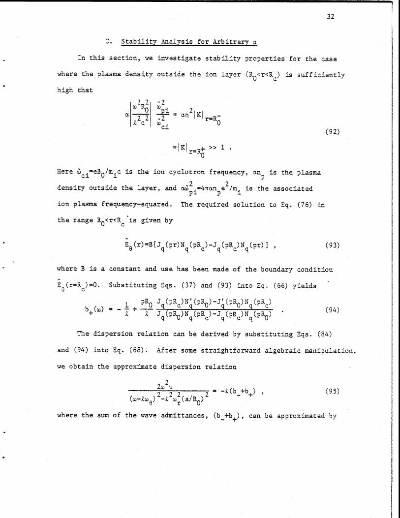
C. Stability Analysis for Arbitrary a

In this section, we investigate stability properties for the case

where the plasma density outside the ion layer (R0<r<Rc) is sufficiently

high that

2 2 A2= 2

2 2 r=RZ c w.c0ci

(92)

= =KI + >> 1 -

0

Here cieB0/M ic is the ion cyclotron frequency, an is the plasma

density outside the layer, and a 2.=4Tran e /m. is the associatedpi p i

ion plasma frequency-squared. The required solution to Eq. (76) in

the range R0<r<Rc is given by

E (r)=B(J (pr)N (pR )-J (pR )N (pr)] , (93)e q q c q c q

where B is a constant and use has been made of the boundary condition

E (r=R c)=0. Substituting Eqs. (37) and (93) into Eq. (66) yields

- +pRQ J (pRc )N (pRo)-J'(pRO)Nq(pR )b+ () = 0 - + q- (94)

+ z z Jq (pR0 )Nq (pR c q (PRc)Nq (pRO)

The dispersion relation can be derived by substituting Eqs. (84)

and (94) into Eq. (68). After some straightforward algebraic manipulation,

we obtain the approximate dispersion relation

2w2 V -Z(b +b (95)

(ZW2_ 22w 2 -aR +(w- )2 r (a/R 0)

where the sum of the wave admittances, (b_+b+), can be approximated by

33

b(w)+b (W) p_R J(p-RO)b_ (o)+b+J (pR)

q- R 0(96)

S +R + (p+RC)N (p+Ro)J (p R)N (p+R)

q+ + 0q)N(p+Rc q+ +Rc) q(P+Ro

In Eq. (96), p_--(w/c)( pi / ci), P+-(W/c)(a/2 pi pci)=n 1/2

2 1/2 2q_=[l+t (2+1/n)] , and q+=(l+Z ( 2+n)]. In deriving Eq. (95), use

has been made of Eqs. (65), (74), and (92). Moreover, in obtaining

the expressions for q+, use has been made of Eq. (77), and w=tZe=

-Z(l+no ci /2. Since the eigenfrequency w is very close to Zc± , we

Taylor-expand the right-hand side of Eq. (95) about w=Zw , retaining

terms to first order in (w-Zw ). After some straightforward algebra,

Eq. (98) can be approximated by

2Zw 22 22 = -[b (w)+b (M)l

((O-zg)2_ 2@ W a/R ) 2 - + W=ZW6r - (97)

- (b_+b+]

2 2where we and Wr (a/R) 2 are defined in Eqs. (78) and (89), respectively.

The growth rate y=Imw and real oscillation frequency Rew have

been obtained numerically from the cubic dispersion relation (97)

for a broad range of system parameters n, w R /c, a, Z, and R /Rc. In

the remainder of this section, we summarize several features of the

stability properties determined from Eq. (97). From Eqs. (41) and (78),

the real frequency Rew can be approximated by

Rew=Zw,=-t(1+n) .c /2 . (98)

The real frequency Rew determined numerically from Eq. (97) is

very close to the value in Eq. (98). In this context, we only

present numerical results for the instability growth rate y.

34

In order to illustrate the dependence of stability properties on

the degree of field reversal, we calculate the wave admittances and

the instability growth rate. Shown in Fig. 6(a) is a plot of

(b_+b+ ) versus n, for 1=2, R /c=4 and a=0. [In the limiting

case of no plasma outside the ion layer (a=0), the dispersion relation

(97) reduces identically to the dispersion relation (90) obtained in

Sec. V.B.] It is evident from Fig. 6(a) that the curves representing

(b +b+ ) become more vertical and the distance between curves

decreases rapidly as q decreases (or, equivalently, as Budker's

parameter v increases). For n<0.3, it is readily shown that (b +b+) W

can be approximated by

(b +b ) =(b_) 2 4(1-")- T (1 + 4/n)1/2

(99)

for the parameters in Fig. 6(a). In obtaining Eq. (99), use has been

1/2made of Eq. (77) and J (x)=(2/rx) cos(x-n7r/2-7r/4) for large x.

Equation (99) provides a good description of the behavior in Fig. 6(a).

In this regard, we do not plot (b +b+) for 1<0.2. Figure 6(b)

shows a plot of the normalized growth rate y/ ci versus r obtained from

Eq. (97) for a=O, R0/R=0.5, a/R0=0.05, and parameters otherwise

identical to Fig. 6(a). Several points are noteworthy in Fig. 6(b).

First, the system is stabilized when the reversal parameter n approaches

zero. This feature has been predicted analytically in Sec. V.B.

Second, the growth rate curve exhibits a repetitive behavior, with the

maximum growth rate for each unstable zone decreasing as I decreases.

Third, the maximum growth rate for each zone occurs at a value of q

corresponding to (b +b+ 0 [Figs. 6(a) and (b)]. Finally, when+

instability does exist, the maximum growth rate can be a substantial

fraction of ion cyclotron frequency ^ci*

35

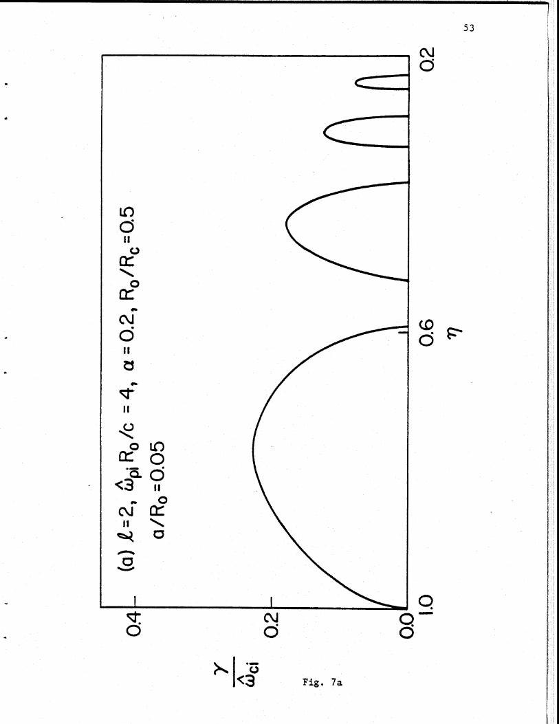
Shown in Fig. 7(a) for Z=2 and in Fig. 7(b) for Z=4 are plots of

normalized growth rate y/wci versus the reversal parameter n [Eq. (97)]

fora=0.2 and parameters otherwise identical to Fig. 6(b). Comparing

Figs. 7(a) and 6(b), we note that the stability properties are almost

identical for a=O and a-0.2, although the maximum growth rate does

decrease slowly as a increases. We therefore conclude that the

influence of plasma outside the layer on stability behavior

is weak, at least when a is sufficiently small (a<0.5, say).

Moreover, we also-note.fromFig. 7 that the width of

the instability zones is reduced for increasing values of azimuthal

harmonic number Z. Furthermore, high-harmonic perturbations are easily

stabilized as q approaches zero.

The dependence of stability properties on plasma density is

illustrated in Fig. 8(a) for Z=2 and in Fig. 8(b) for Z=4, where the

normalized growth rate y/ ci is plotted versus w R0/c for n=0.82

and parameters otherwise identical to Fig. 7. Note that the growth

rate is a decreasing function of 2 R /c. This feature is also evident

from Eqs. (87) and (90) for a=0. We further note from Fig. 8(b)

that the system is completely stabilized above some critical value of

W R /c. For example, from Fig. 8(b), the Z=4 perturbation is stable

for R /c,7. In this regard, we conclude that the layer-plasmapi 0 /cV7

configuration can be completely stabilized provided the plasma density

is sufficiently high.

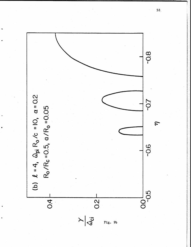
Of considerable interest for experimental application is the stability

behavior for a field-reversed configuration with n<O. Figure 9 shows

a plot of normalized growth rate versus n obtained from Eq. (97) for

Z=2 [Fig. 9(a)] and Z=4 [Fig. 9(b)], and equilibrium parameters

WiR/c=10, a=0.2, R0 /RC=0.5, and a/R0=0.05. As discussed in Sec. V.B,

36

for n<O, Eq. (97) is valid only when -l<n<- 22 /(1+2. ) [Eq. (82)],

and KI r=R->>1L. Moreover, the electromagnetic coupling parameter0

K=R~ decreases to zero when n approaches minus unity. In this regard,0

the plots in Fig. 9 are presented only for the range -0.85<n<-0.5.

We note from Figs. 9(a) and 9(b) that the instability growth rate

decreases considerably as Inl approaches 0.5. The stabilization

for low value of Inj is associated with finite beta electromagnetic

effects. Moreover, this stabilization is most pronounced for high

azimuthal harmonic numbers [compare Figs. 9(a) and (b)]. We conclude

from Figs. 7 and 9 that the system is most stable when the magnetic

compression ratio n approaches zero.

37

VI. NUMERICAL ANALYSIS OF STABILITY PROPERTIES FOR

ARBITRARY VALUES OF BACKGROUND PLASMA DENSITY

In this section, we investigate the stability properties numerically

for arbitrary values of background plasma density, assuming a rectangular

density profile with a = 0. As shown in Sec. V.A, the eigenfunction $(r)

for arbitrary n satisfies Eq. (72) at all radial locations, except at

r = R0 . Since the stability analysis in this section is limited to a = 0,

the wave admittance b+ is given by Eq. (81). However, in order to determine

the wave admittance b in the region 0 < r < R0, it is necessary to solve

the eigenvalue equation (72), which is a simple second-order differential

equation with boundary conditions $(r-0) = (d$/dr) r= = 0 at r = 0.

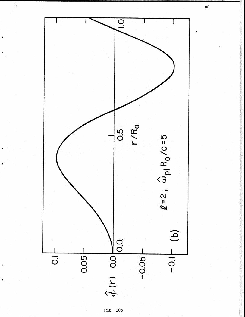
The eigenfunction $(r) has been calculated numerically Eq. (72) for

Z = 2 and w=-M , which corresponds to full reversal with n = 1. Shown in

Fig. 10 are the corresponding plots of $(r) versus r/R0 for (a) w R0 /c=l,

(b) w .R0/c=5, and (c) w .R /c=10. It is evident from Fig. 10(a) that thepi pi

electrostatic eigenfunction p(r) = (r/R 0 is a very good approximation for

a low-density background plasma satisfying w R /c < 1. However, for a

high-density background plasma with w .R /c > 1, the eigenfunction exhibitspi0

oscillatory (Bessel-function-like) behavior, which indicates the important

influence of electromagnetic effects associated with background plasma

dielectric properties [Fig. 10(b) and (c)]. Moreover, the eigenfunction

oscillates rapidly as a function of increasing plasma density. In order to

illustrate the dependence of the wave admittance b = R0(d/dr)R R 0) on

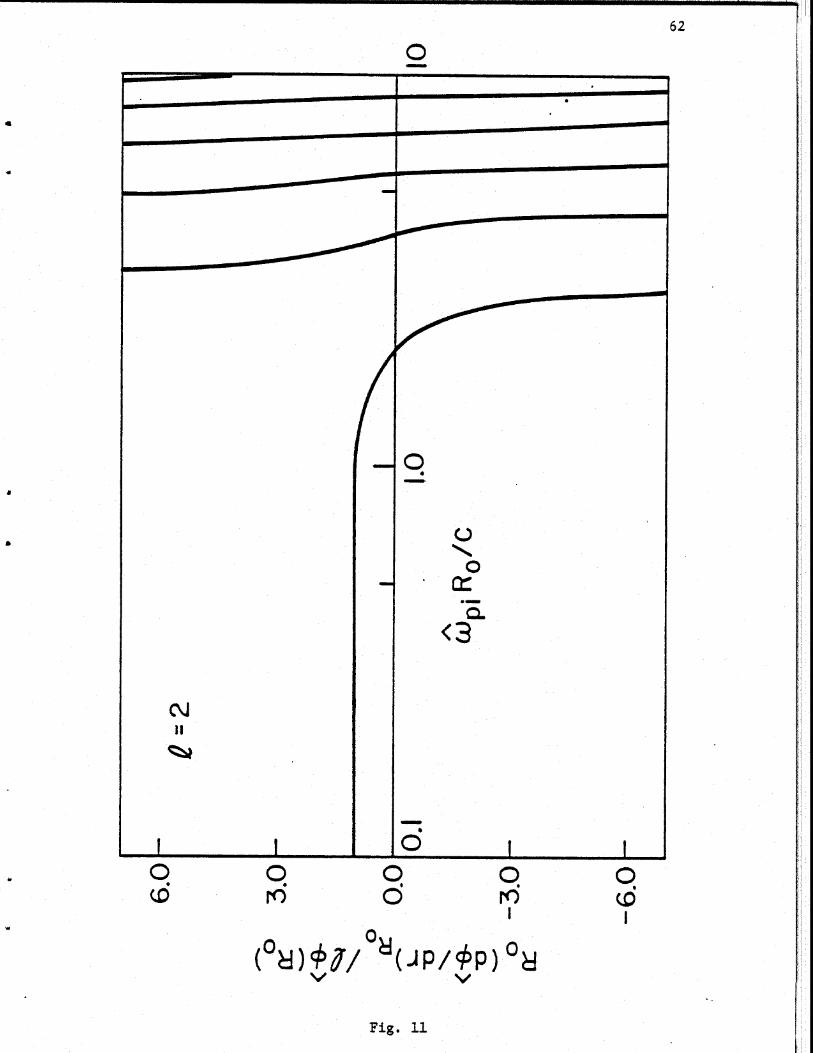
plasma density, Fig. 11 shows a plot of b_ versus R 0/c for Z=2 and n=l.

Evidently, from Fig. 11, the wave admittance b_ is approximately equal to

unity in the range 0 < w R /c<l, thereby ensuring that the electrostatic

38

approximation is valid for a low-density background plasma. On the other

hand, it is also clear from Fig. 11 that electromagnetic effects are very

important for plasma densities satisfying w .R /c / 2.pi 0

The dependence of stability properties on plasma density is illustrated

in Fig. 12, where the normalized growth rate Y/wci is plotted versus

W R /c for Z=2, and n=0.95[Fig. 12(a)] and n= -0.9 (Fig. 12(b)]. In Fig. 12(a),

the stability properties are very similar to the results obtained analytically

in Fig. 8(a). Moreover, for a highly field-reversed layer [Fig. 12(b)],

it is evident that the instability can be completely stabilized by increasing

the plasma density beyond a certain critical value [w R 0/c=20.5 in Fig. 12(b)].

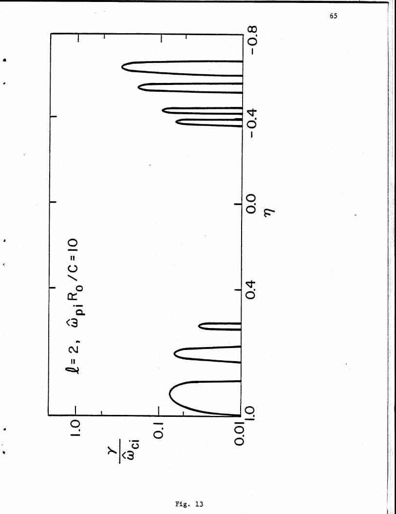
Shown in Fig. 13 is a plot of growth rate y/w . versus n for Z=2 and

W R /c=10. As expected from the analytic results in Figs. 7(a) and 9(a),

for nIj0.4, the instability is completely stabilized by the effects of

finite transverse temperature of the layer ions. Finally, comparing Figs.

12 and 13 with the results obtained analytically in Sec. V.C, we conclude that

the analytic studies in Sec. V.C give a good qualitative description of

stability behavior.

39

VII. CONCLUSIONS

In this paper, we have investigated the electromagnetic stability

properties of an intense P-layer immersed in a dense plasma background.

The equilibrium and stability analysis was carried out within the frame-

work of a hybrid Vlasov-fluid model in which the background plasma elec-

trons and ions are described as macroscopic, cold fluids confined by the

0axial magnetic field B (r)e and the layer ions are described by the

Z MZ

Vlasov equation. Moreover, the equilibrium and stability properties were

calculated for the' case in which the background plasma has a step-function

density profile and the layer ions are described by the rigid-rotor distri-

bution function in Eq. (2). Various equilibrium properties were calculated

in Sec. II. One of the most important features in the equilibrium analysis

for a thin layer is that Budker's parameter V for the layer ions is directly

related to the magnetic compression ratio n by v=(l-n)/(l+n). Electromag-

netic stability properties were investigated in Secs. III-VI, assuming that

all perturbed quantities are independent of axial coordinate (/9z=O). A

formal stability analysis was carried out in Sec. IV. Equation (69), when

combined with Eq. (68), constitute one of the main results of this paper

and can be used to investigate stability properties for a broad range of

system parameters. A detailed analytic and numerical investigation of

electromagnetic stability properties was carried out in Sec. V for a dense

background plasma and in Sec. VI for arbitrary values of background plasma

density. It was found that the effects of (a) the equilibrium magnetic

field depression produced by the P-layer, (b) transverse magnetic perturba-

tions (SB#O), (c) small (but finite) transverse temperature of the layer

ions, and (d) the dielectric properties of the background plasma, all have

40

an important influence on stability behavior. For example, for a dense

background plasma, the system can be easily stabilized by a sufficiently

large transverse temperature of the layer ions.

ACKNOWLEDGMENTS

This research was supported by the National Science Foundation. The

research by one of the authors (H.S.U.) was supported in part by the Office

of Naval Research.

dMOWNWAMMMiNew

41

APPENDIX A

EVALUATION OF PERTURBED CHARGE DENSITY FOR THE LAYER IONS

To complete the stability analysis, in this Appendix we evaluate

the perturbed charge density associated with the layer ions. Combining

Eqs. (3) and (43), it is straightforward to show that the radial equation

of motion for the layer ions is given by

r'-r=(v±/Wr)[cos(WrT-a)-cosa] , (A.1)

where T=t'-t, v. is the perpendicular speed in a frame of reference

rotating with angular velocity w , cosa=(v -rw )/v±, and r' and r

are the radial distances of the particles from the z-axis at times t'=t'

and t'=t, respectively. The time derivative of Eq. (A.1) gives the

radial velocity,

v'=v (sinacoswTr-cosasinwr) , (A.2)

for the layer ions.

Consistent with Eq. (1), the perturbed distribution function for

a thin ion layer can be expressed as,

0

fb (r,v)=e dT exp{-i(r-Z(e'-6)1}

(A.3)

x { I cosa iZ;(Ro) + R v R 0 R]

where use has been made of Eqs. (38), (40), and (42). Since the

variable (W'-6) in Eq. (A.3) is a function of cosa, it follows from

Eqs. (46), (A.2), and (A.3) that any term in the time integration in

Eq. (A.3) that is a function of sina will give zero when the integration

over a is carried out. In this context, we can replace Eq. (A.2) by

42

V =-V4 cosasinrT , (A.4)

without loss of generality in the present analysis. For low-frequency

(WL"e) perturbations, consistent with Eqs. (41) and (63), it is valid

to neglect the term proportional to B z(R0) in Eq. (A.3), since the

corrections associated with this term are of order -ZW Zel/ ci («1)

or smaller than the corrections associated with the term proportional

to (3a/3r) in Eq. (A.3). This can be easily verified by making use

of Eqs. (36), (55), and (A.4). Substituting Eq. (A.4) into Eq. (A.3),

we obtain an approximate expression for the perturbed distribution

function,

V, af 00

f bl(r,v)=iek cos a dT exp{-i(WT -Z(6 '-6) ]}

(A.5)

x ;(R0 )+ R /22 [exp(i T)-exp T)

The perturbed surface charge density abZ for a very thin ion

layer is evaluated by substituting Eqs. (42) and (A.5) into Eq. (46).

After some straightforward algebra, we obtain

_ 2 2 $(R0 ) 2R0 a

R 0 (W-z )2Z2w (a/R)2+ 2- 0r R W r

(A.6)

where use has been made of Eq. (41). From Eq. (A.6), it is easily

shown that the correction associated with the term proportional to

(90/;r)R is negligibly small except when RO(a/9 R /c(R0)t-ow.0 0

In this context, we conclude that the perturbed surface charge density

a b for a thin ion layer can be approximated by,

1 2 c 2;(R )/R3b = -2(A.7)b 27 (Wz 2 2 w2(a/R0) 2

43

REFERENCES A

1. H. A. Davis, R. A. Meger, and H. H. Fleischmann, Phys. Rev. Lett.

37, 542 (1976).

2. S. C. Luckhardt and H. H. Fleischmann, Phys. Rev. Lett. 39,

747 (1977).

3. R. N. Sudan and E. Ott, Phys. Rev. Lett. 33, 355 (1974).

4. C. A. Kapetanakos, J. Golden, and K. R. Chu, Plasma Phys. 19,

387 (1977).

5. H. A. Davis, H. H. Fleischmann, R. E. Kribel, D. Larrabee, R. V.

Lovelace, S. C. Luckhardt, D. Rej, and M. Tuszewski, in Proceedings

2nd International Topical Conference on High Power Electron and Ion

Beam Research and Technology (Ithaca, N. Y. 1977), Vol. I, p. 423.

6. C. A. Kapetanakos, J. Golden, Adam Drobot, R. A. Mahaffey, S. J.

Marsh, and J. A. Pasour, in Proceedings 2nd International Topical

Conference on High Power Electron and Ion Beam Research and Technology

(Ithaca, N. Y. 1977), Vol. I, p. 435.

7. A. Mohri, K. Narihara, T. Tsuzuki, and Y. Kubota, in Proceedings 2nd

International Topical Conference on High Power Electron and Ion

Beam Research and Technology (Ithaca, N. Y. 1977), Vol. I, p. 459.

8. D. E. Baldwin and 11. E. Rensink, Comments on Plasma Physics and

Controlled Fusion, in press (1978).

9. R. V. Lovelace, Phys. Rev. Lett. 35, 162 (1975).

10. R. N. Sudan and M. N. Rosenbluth, Phys. Rev. Lett. 36, 972 (1976).

11. H. Uhm and R. C. Davidson, Phys. Fluids 20, 771 (1977).

12. H. S. Uhm and R. C. Davidson, Phys. Fluids 21, 265 (1978).

13. H. S. Uhm and R. C. Davidson, "Stability Properties of a Cylindrical

Rotating P-Layer Immersed in a Uniform Background Plasma", submitted

for publication (1978).

44

FIGURE CAPTIONS

Fig. 1 Equilibrium configuration and coordinate system.

Fig. 2 Density profile [Eq. (9) ] for the layer ions.

Fig. 3 Axial magnetic field profile [Eq. (14)].

Fig. 4 Sketch of the envelope function i(r) versus r (Eq. (11)]

with t(R)=O=ip(R 2) and [3/Dr] r=RO

Fig. 5 Electron and ion density profiles [Eq. (44)] for the background

plasma.

Fig. 6 Plots of (a) sum of wave admittances (b_+b+ )o [Eq. (96)]A 6

and (b) normalized growth rate y/wci [Eq. (97)] versus n for

Z=2, wRO/c-4, ca=O, RO/RC=0.5 and a/Ro=0.05.

Fig. 7 Plot of normalized growth rate y/c versus n [Eq. (97)] for

a=0.2. Cases shown are for (a) t=2 and (b) Z=4, and parameters

otherwise identical to Fig. 6.

Fig. 8 Plots of normalized growth rate y/ ci versus wpR 0 /c [Eq. (97)]

for (a) Z=2 and (b) Z=4, with I=O..82 and parameters otherwise

identical to Fig. 7.

Fig. 9 Plots of normalized growth rate y/Ici versus n [Eq. (97)]

for (a) Z=2. and (b) Z=4, with w R /c=10, a=0.2, R /RC=0.5pi 0 0c

and a/R0=0.05.

Fig. 10 Plot of eigenfunction 0(r) versus r/R [Eq. (72)] for t=2,

n=l and (a) w R 0/c-l, (b) w Ro/c=5, and (c) W RO/c=l0.

wig. 11 Plot of wave admittance b =R0 (d$/dr)R /Z$(Ro) versus0

c pi R /c for Z=2 and n=l.

45

Fig. 12 Plot of Normalized growth rate y/wi versus w RO/c for Z=2,

and (a) n=0.95, (b) n= -0.9.

Fig. 13 Plot of growth rate y/wci versus I for Z=2 and w R /c=10.

46

N

-D

-Jz

o

z0

<A

/I

Ns

ON

0c"J

Fig. 1

I z

C-)

00

47

- - -- - - -- - - I

_ I _ _V R1

r

Fig. 2

j .

0

48

7 8

41

v Rl R2

Fig. 3

49

0

01

Fig. 4

CONDUCTING WALL

.5

CLc

1 0a

50

0

0S -mmm - -

0. 0

Fig. 5

C\J0

0

0

(+q+ -q)Fig. 6a

51

II

0

0

<3

('411

0lI

0

I

I

00 11111

wd

k.) LO

czII

0

0

It

ii

0

.a qeN0

3 \

0

I00-

0

Fig. 6b

52

N~0

0D

0

I

p

53~

N\0

0

0

CM (od

11

00

0

C;

C\J 000 0-

1<3Fig. 7

clii

0d

Fig. 7b

54

OII

0C

c~j

0

0

1.

.;

C3

dC\jd

C\j

0

I

55

cco

C\JO 0

C

0t 0

CO~

01 0

1< Fig. 8a

0~j0if0

N

3

I I

0 C\j0

56

~cz

~z2II(0

C0'4

0

<3-

Ir,0d

Fig. 8b>,. Jg

(::::i-

57

c~co0d

LO 0j0

0. d

n,,

d 05

Fig. 9a

53

c~co00

0I

0

000

0

LO

00

00

00 01

Fig. 9b

59

0

~~~~10U'

L

Fig. 10a

0

C\j

0*

0

L

q0

---a

I I I

0 0

0

LO

0

<3

60

LCdi

c\JII

0,0; I

00

nC0d

0

Fig. 10b

I I

I

3

0

0

N.3a

<:3

N~0ci

I

N0ci

Fig. 10c

61

0di

0ci 0

ci

0

62

0

0

0

0ni

op 0 .Jp/p) 0%ve v

Fig. 11

04ii

<0 0ro

I I

0 0(:

I I

63

0

0di

QI

Fig. 12a

1O

C %J11

rO6 05

I I I

00 c0

Q0

- I

NlI

0

Fig. 12b

64

Nd

CC

0

CrJ

0C\J

)-W6-

0

0

0.

C~4j

Z710, --

I

Fig. 13

65

I I

00

I

-Q

..

---