Stable seismic data recovery - University of British … · wavefronts & reflectors are multiscale...

Stable seismic data recovery

Felix J. Herrmann*joint work with

Peyman Moghaddam*, Gilles Hennenfent* & Chris Stolk (Universiteit Twente)

*Seismic Laboratory for Imaging and Modeling

slim.eos.ubc.caAIP 2007, Vancouver, June 26

Combinations of parsimonious signal representations with nonlinear sparsity promoting programs hold the key to the next-generation of seismic inversion algorithms ...Since they allow for formulations that are stable w.r.t.

noise incomplete data moderate phase rotations and amplitude errors

Finding a sparse representation for seismic data & images is complicated because of

wavefronts & reflectors are multiscale & multi-directional

the presence of caustics, faults and pinchouts the presence of operators (FIO’s & PsDO’s)

The seismic method

0

1

2

3

4

time [

s]

-3000 -2000 -1000offset [m]

Seismic data acquisition

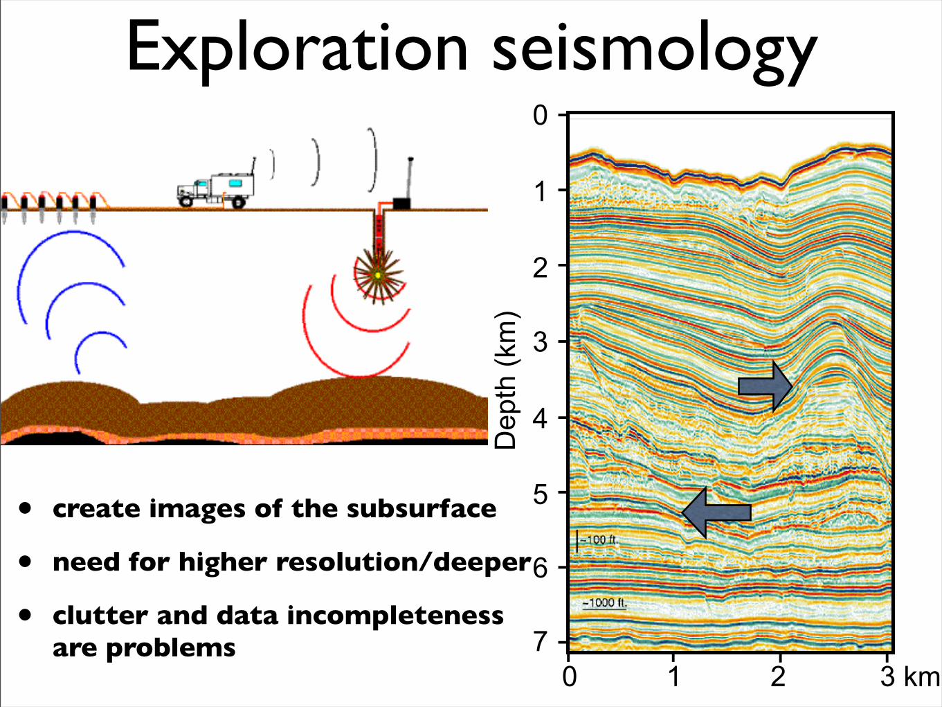
Exploration seismology

• create images of the subsurface

• need for higher resolution/deeper

• clutter and data incompleteness are problems

0 1 2 3 km

0

1

2

3

4

5

6

7

Dep

th (k

m)

Forward problem

• second order hyperbolic PDE

• interested in the singularities of

F [c]u :=

!1

c2(x)· !2

!t2!

d"

i=1

!2

!x21

#u(x, t) = f(x, t)

m = c! c

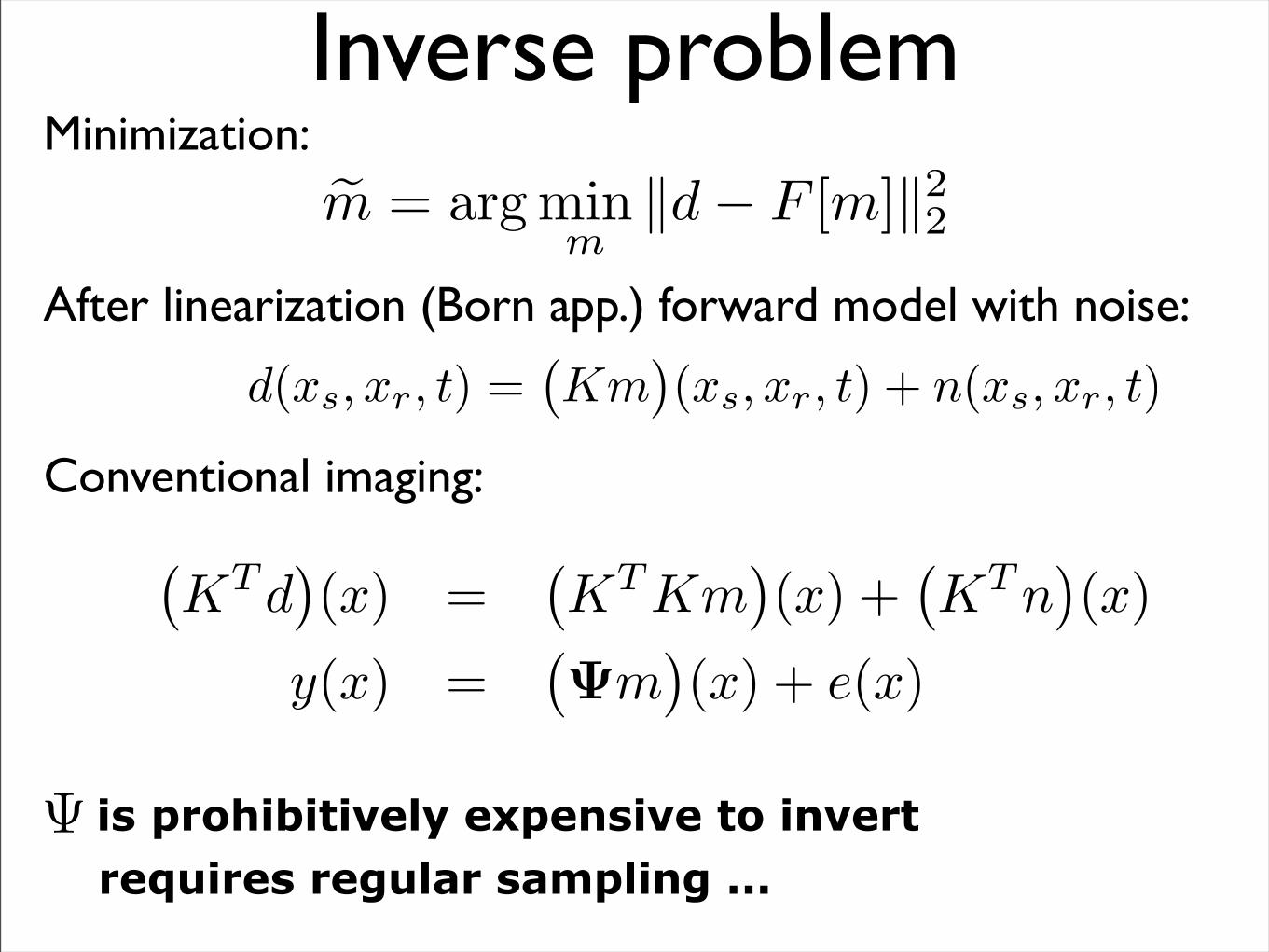
Inverse problemMinimization:

After linearization (Born app.) forward model with noise:

Conventional imaging:

is prohibitively expensive to invert requires regular sampling ...

!m = arg minm

!d" F [m]!22

d(xs, xr, t) =!Km

"(xs, xr, t) + n(xs, xr, t)

!KT d

"(x) =

!KT Km

"(x) +

!KT n

"(x)

y(x) =!!m

"(x) + e(x)

!

Sparsity promoting inversion

Formulate as inverse problem

x = arg minx

!x!1 s.t. !Ax" y!2 # !

data misfitsparsityenhancement

When a traveler reaches a fork in the road, the l1 -norm tells him to take either one way or the other, but the l2 -norm instructs him to head off into the bushes.

John F. Claerbout and Francis Muir, 1973

New field “compressive sampling”: D. Donoho, E. Candes et. al., M. Elad etc.

Preceded by others in geophysics: M. Sacchi & T. Ulrych and co-workers etc.

signal =y + n noise

curvelet representation of ideal data

x0

A

Sparsity promoting inversion can be recovered by solving

Crux lies in finding the sparse representation!

x0

P! :

!x = arg minx !x!1 s.t. !Ax" y!2 # !

f = ST xwith

y = (incomplete) dataA = modeling matrix, e.g.A = RST

x = recovered sparsity vector! = a number dependent on the noise level

ST = the synthesis matrixf = the recovered function f

Curvelets & seismology

Wish listTransform that is parsimonious

detects the wavefronts localized in space and frequency (phase space) some invariance under “wave propagation”

Events correspond to curved singularities with conflicting dips

caustics faults & pinch outs

Need a transform that is multiscale multidirectional exactly reconstructs

Properties curvelet transform: multiscale: tiling of the FK domain into

dyadic coronae multi-directional: coronae sub-

partitioned into angular wedges, # of angle doubles every other scale

anisotropic: parabolic scaling principle Rapid decay space Strictly localized in Fourier Frame with moderate redundancy

Transform Underlying assumption

FK plane waves

linear/parabolic Radon transform linear/parabolic events

wavelet transform point-like events (1D singularities)

curvelet transform curve-like events (2D singularities)

k1

k2angular

wedge2j

2j/2

Representations for seismic data

fine scale data

coarse scale data

2-D curvelets[Candes, Donoho, Demanet, Ying]

curvelets are of rapid decay in space

curvelets are strictly localized in frequency

x-t f-kOscillatory in one direction and smooth in the others!

0

0.5

1.0

1.5

2.0

Tim

e (s

)

-2000 0 2000Offset (m)

0

0.5

1.0

1.5

2.0

Tim

e (

s)

-2000 0 2000Offset (m)

Significantcurvelet coefficient Curvelet

coefficient~0

Wavefront detection

curvelet coefficient is determinedby the dot product of the curveletfunction with the data

Compression

[From Demanet ‘05][From Demanet ‘05]

Curvelets live in wedges in the 3 D Fourier plane...

3-D curvelets

Nonlinear approximation

Curvelet-based seismic data recovery

joint work with Gilles Hennenfent

Sparsity-promoting inversion*Reformulation of the problem

Curvelet Reconstruction with Sparsity-promoting Inversion (CRSI)

look for the sparsest/most compressible,physical solution KEY POINT OF THE

RECOVERY

* inspired by Stable Signal Recovery (SSR) theory by E. Candès, J. Romberg, T. Tao, Compressed sensing by D. Donoho & Fourier Reconstruction with Sparse Inversion (FRSI) by P. Zwartjes

signal =y + n noise

curvelet representation of ideal data

x0

RCH

(P0)

!

""""#

""""$

x= arg

sparsity constraint% &' (

minx

!x!0 s.t. !y"PCHx!2 # !

f= CH x

(P0)

!

""""#

""""$

x= arg

sparsity constraint% &' (

minx

!x!0 s.t.

data misfit% &' (

!y"PCHx!2 # !

f= CH x

P! :

!x = arg minx !Wx!1 s.t. !Ax" y!2 # !

f = CT x

Original data

85 % missing

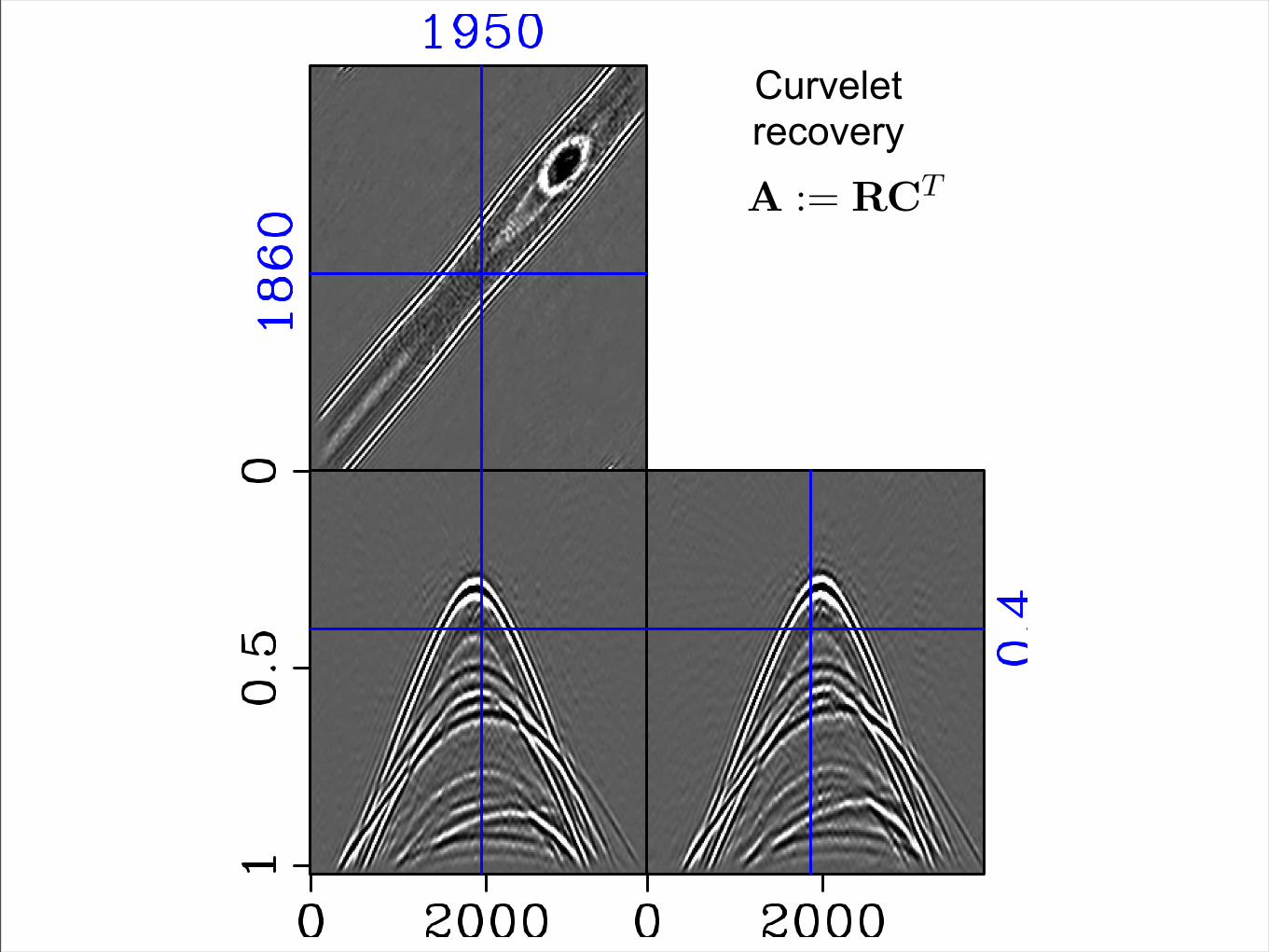
Curvelet recovery

SEISMIC DATA RECOVERY

The reconstruction of seismic wavefields from regularly-sampled data with missing traces

is a setting where a curvelet-based method will perform well (see e.g. Herrmann, 2005;

Hennenfent and Herrmann, 2006a, 2007). As with other transform-based methods, sparsity

is used to reconstruct the wavefield by solving P!. It is also shown that the recovery

performance can be increased when information on the major primary arrivals is included

in the modeling operator.

Curvelet-based recovery

The reconstruction of seismic wavefields from incomplete data corresponds to the inversion

of the picking operator R. This operator models missing data by inserting zero traces at

source-receiver locations where the data is missing. The task of the recovery is to undo this

operation by filling in the zero traces. Since seismic data is sparse in the curvelet domain,

the missing data can be recovered by compounding the picking operator with the curvelet

modeling operator, i.e., A := RCT . With this definition for the modeling operator, solving

P! corresponds to seeking the sparsest curvelet vector whose inverse curvelet transform,

followed by the picking, matches the data at the nonzero traces. Applying the inverse

transform (with S := C in P!) gives the interpolated data.

An example of curvelet based recovery is presented in Figure 1, where a real 3-D seismic

data volume is recovered from data with 80 % traces missing (see Figure 1(b)). The missing

traces are selected at random according to a discrete distribution, which favors recovery (see

e.g. Hennenfent and Herrmann, 2007), and corresponds to an average sampling interval of

125 m . Comparing the ’ground truth’ in Figure 1(a) with the recovered data in Figure 1(c)

5

ObservationsInverted a rectangular matrix

worked because the curvelet transform is sparse exploits the higher dimensional geometry of

seismic wavefields curvelets are incoherent with the Dirac

measurement basis

Data is recovered for large percentages of traces missingIs an example of an inverse problem with incomplete dataCan these ideas be extended to recover migration amplitudes?

approximately invert a PsDO diagonalize zero-order PsDO’s

Stable seismic amplitude recovery

“Sparsity- and continuity-promoting seismic image recovery

with curvelet frames”

by

F.H, P. Moghaddam & C. Stolk

to appear in special issue on imaging in ACHA

Seismic Laboratory for Imaging and Modeling

Migrated data Amplitude-corrected & denoised migrated data

Existing scaling methodsMethods are based on a diagonal approximation of .

Illumination-based normalization (Rickett ‘02) Amplitude preserved migration (Plessix & Mulder ‘04) Amplitude corrections (Guitton ‘04) Amplitude scaling (Symes ‘07)

We are interested in an ‘Operator and image adaptive’ scaling method which

estimates the action of from a reference vector close to the actual image

assumes a smooth symbol of in space and angle does not require the reflectors to be conormal <=>

allows for conflicting dips stably inverts the diagonal

!

!

!

Our approach“Forward” model:

diagonal approximation of the demigration-migration operator

costs one demigration-migration to estimate the diagonal weighting

withy = migrated dataA := CT !

AAT r ! KT KrK = the demigration operator! = migrated noise.

y = KT Km + !

! Ax0 + !

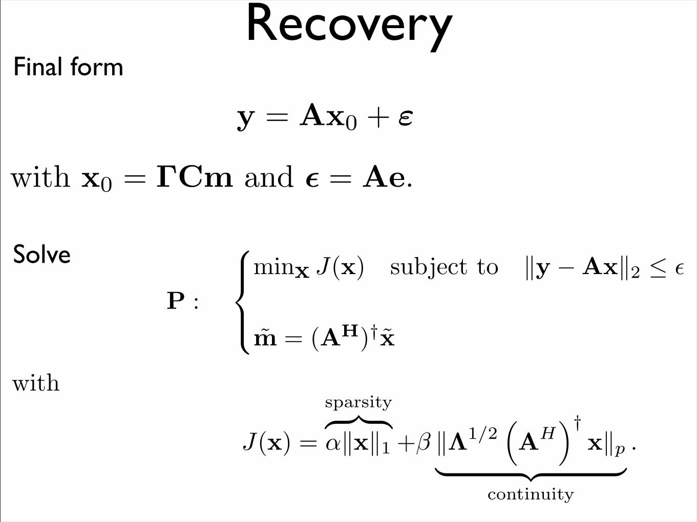
SolutionSolve

need sparsity on the model invariance under the normal operator

P :

!"#

"$

minx J(x) subject to !y "Ax!2 # !

m = (AH)†x

with

J(x) =

sparsity% &' ("!x!1 +# !!1/2

)AH

*†x!p

' (% &continuity

.

Nonlinear approximationMigrated mobil data set

Nonlinear approximationRecovery from largest 3 %

Nonlinear approximationDifference

Diagonal approximation of the Hessian

Normal/Gramm operator[Stolk 2002, ten Kroode 1997, de Hoop 2000, 2003]

In high-frequency limit is a PsDO

• pseudolocal

• singularities are preserved

Inversion corrects for the ‘Hessian’

!!!f

"(x) =

#

Rde!ix·!a(x, !)f(!)d!

• curvelets remain invariant

• approximation improves for higher frequencies

(a) (b) (c) (d)

(e) (f) (g) (h)

Figure 2: Invariance of curvelets under the discretized normal operator Ψ for a smoothly

varying background model (a so-called lens model see Fig. 4(a)). Three coarse-scale

curvelets in the physical domain before (a) and after application of the normal opera-

tor (b) in the physical (a-b) and Fourier domain (e-f). The results for three fine-scale

curvelets are plotted in (c-d) for the physical domain and in (g-h) for the Fourier domain.

Remark: The curvelets remain close to invariant under the normal operator, a statement

which becomes more accurate for finer scale which is consistent with Theorem 1. The ex-

ample also shows that this statement only holds for curvelets that are in the support of the

imaging operator excluding steeply dipping curvelets.

52

(a) (b) (c) (d)

(e) (f) (g) (h)

Figure 2: Invariance of curvelets under the discretized normal operator ! for a smoothly

varying background model (a so-called lens model see Fig. 4(a)). Three coarse-scale

curvelets in the physical domain before (a) and after application of the normal opera-

tor (b) in the physical (a-b) and Fourier domain (e-f). The results for three fine-scale

curvelets are plotted in (c-d) for the physical domain and in (g-h) for the Fourier domain.

Remark: The curvelets remain close to invariant under the normal operator, a statement

which becomes more accurate for finer scale which is consistent with Theorem 1. The ex-

ample also shows that this statement only holds for curvelets that are in the support of the

imaging operator excluding steeply dipping curvelets.

52

Invariance under Gramm matrix

So let ! = !(x,D) be a pseudodi!erential operator of order 0, with homo-geneous principal symbol a(x, !).

in Rd.

Lemma 1. With C ! some constant, the following holds

!(!(x,D)" a(xν , !ν))"ν!L2(Rn) # C !2"|ν|/2. (14)

To approximate !, we define the sequence u := (uµ)µ#M = a(xµ, !µ). Let D! be the

diagonal matrix with entries given by u. Next we state our result on the approximation of

! by CTD!C.

Theorem 1. The following estimate for the error holds

!(!(x,D)" CTD!C)"µ!L2(Rn) # C !!2"|µ|/2, (15)

where C !! is a constant depending on !.

This main result proved in Appendix A shows that the approximation error for the

diagonal approximation goes to zero for increasingly finer scales. The approximation derives

from the property that the symbol is slowly varying over the support of a curvelet, an

approximation that becomes more accurate as the scale increases.

Decomposition of the normal operator

By virtue of Theorem 1, the normal operator can be factorized

!!"µ

"(x) $

!CTD!C"µ

"(x) (16)

=!AAT "µ

"(x)

with A :=%

D!C and AT := CT%

D!. Because the seismic reflectivity can be written as a

superposition of curvelets, we can replace "µ in the above equation with the model m. We

15

leading behavior for their composition, the normal operator !, corresponds to that of an

order-one invertible elliptic PsDO .

To make this PsDOamenable to an approximation by curvelets, the following sub-

stitutions are made for the scattering operator and the model: K !" K (#")!1/2 and

m !" (#")1/2 m with ((#")!f)"(!) = |!|2! · f(!). Alternatively, these operators can be

made zero-order by composing the data side with a 1/2-order fractional integration along

the time coordinate, i.e., K !" "!1/2t K (see e.g. 3). After these substitutions, the normal

operator ! becomes zero-order. Remark that these subsitutions are similar to the substi-

tution made in the WVD methods, where vaguelettes are introduced according the same

mappings. Before detailing the approximate diagonalization of the normal operator, we

first discuss the properties of continuous curvelets under this operator.

APPROXIMATION OF THE NORMAL OPERATOR

In this section, a diagonal approximation of the normal operator in the curvelet domain is

presented. Invariance properties of curvelets under the normal operator (see also Fig. 2)

are used. The approximation leads to a SVD-like decomposition of the normal operator

and makes large-scale seismic image recovery amenable to optimization. To understand our

approximation, we first list the important properties of continuous curvelets. An upper

bound for the L2-error of the diagonal approximation is discussed next, followed by the

diagonal decomposition of the normal operator and a method to numerically estimate the

diagonal from discrete implementations of the normal operator. We conclude this section

by discussing the empirical performance of the approximation on a synthetic data set.

11






















11






















11






















11

orwith

Approximation

• Allows for the decomposition

in Rd.

Lemma 1. With C ! some constant, the following holds

!(!(x,D)" a(x! , !!))"!!L2(Rn) # C !2"|!|/2. (14)

To approximate !, we define the sequence u := (uµ)µ#M = a(xµ, !µ). Let D! be the

diagonal matrix with entries given by u. Next we state our result on the approximation of

! by CTD!C.

Theorem 1. The following estimate for the error holds

!(!(x,D)" CTD!C)"µ!L2(Rn) # C !!2"|µ|/2, (15)

where C !! is a constant depending on !.

This main result proved in Appendix A shows that the approximation error for the

diagonal approximation goes to zero for increasingly finer scales. The approximation derives

from the property that the symbol is slowly varying over the support of a curvelet, an

approximation that becomes more accurate as the scale increases.

Decomposition of the normal operator

By virtue of Theorem 1, the normal operator can be factorized

!!"µ

"(x) $

!CTD!C"µ

"(x) (16)

=!AAT "µ

"(x)

with A :=%

D!C and AT := CT%

D!. Because the seismic reflectivity can be written as a

superposition of curvelets, we can replace "µ in the above equation with the model m. We

15

!!!µ

"(x) !

!CT D!C!µ

"(x)

=!AAT !µ

"(x)

with A :=!

D!C and AT := CT!

D!.

Approximation

y(x) =!!m

"(x) + e(x)

!!AAT m

"(x) + e(x)

= Ax0 + e,

Approximation

Wavelet-vagulette likeAmenable to nonlinear recovery

Estimation of the diagonal scaling

• Define a reference vector (say conventional image).

• Calculate ‘data’

• Define the matrix

• Invert

b = !r

v = CrP := CT diag(v) with

u = arg minu12!b"Pu!2

2 + !2!Lu!22

Diagonal estimation

• Impose smoothness in phase space

L = [D1 D2 D!]

extended to include q di!erent reference vectors by making the following substitutions

b !" [b1 · · · bq]T and P !" [P1 · · · Pq]T with the “data” vector and “modeling” matrix

defined by the di!erent reference vectors r1, . . . , rq.

Calculate: b = !r and v = Cr.

Set: ! = !min;

while # (uµ)µ!M < 0 do

Solve

!u = arg minu12$b%Pu$22 + !2$Lu$22

Increase the Lagrange multiplier

" = ! + "!

end while

Table 1: Estimation of the diagonal via regularized least-squares inversion. The Lagrange

multiplier is increased up to the point that all entries in the vector for the diagonal are

positive.

Given an appropriate reference vector r, the diagonal estimation procedure is as follows.

First, calculate the action of the normal operator on the reference vector and the curvelet

transform of this vector. Next we set the Lagrange multiplier to !min and solve Eq. (17)

for this ! by inverting the system of equations in Eq. (18). The ! is increased by "! until

all diagonal elements of !u are nonnegative. Even though we do not have a proof for the

connvergence of this method, in practice increasing the ! leads to positive entries.

The presented method for the estimation for the diagonal can be seen as an extension

to the method of illumination-based normalization (33), dating back to ideas by Symes and

19

Diagonal estimation

(a) (b)

(c) (d)

Figure 5: Estimates for the diagonal !u are plotted in (a-d) for increasing ! =

{0.01, 0.1, 1, 10}. The diagonal is estimated according the procedure outlined in Table 1

with the reference and ’data’ vectors, v and b, plotted in Fig. 4(b) and 4(c). As expected

the diagonal becomes more positive for increasing !.

Herrmann et.al. –

54

Diagonal estimation

Seismic amplitude recovery

• Final form

• Solve

y = Ax0 + !

Recovery

with x0 = !Cm and ! = Ae.

P :

!"#

"$

minx J(x) subject to !y "Ax!2 # !

m = (AH)†x

with

J(x) =

sparsity% &' ("!x!1 +# !!1/2

)AH

*†x!p

' (% &continuity

.

Image recoveryanisotropic diffusion

[Black et. al ’98, Fehmers et. al. ’03 and Shertzer ‘03]

Define

with p=2

Jc(m) = !!1/2!m!p

The anisotropic-di!usion penalty term (see e.g. 24) is given by

Jc(m) = !!1/2!m!22 (28)

with ! the discretized gradient matrix defined as ! =!DT

1 DT2

"T . The block-diagonal

matrix ! is location dependent (see Fig. 10, which plots the gradients) and rotates the

gradient towards the tangents of the reflecting surfaces. This rotation matrix is given by

![r] =1

!!r!22 + 2!

#$$%

$$&

'

(()+D2r

"D1r

*

++,

-+D2r "D1r

.+ !Id

/$$0

$$1(29)

with Di the discretized derivative in the ith coordinate direction and ! a parameter that

controls the fluctuations for regions where the gradient is small. Following (3), this control

parameter is set proportional to the median of |!r| with | | the length of each gradient

vector (white arrows in Fig. 10). Similar to the diagonal approximation, a reference vector

derived from the migrated image (cf. Eq. 24) is used to calculate the tangential directions

of the reflecting surfaces.

By combining the two di!erent penalty terms that promote sparsity and continuity, we

finally arrive at our approximate formulation for the seismic-amplitude recovery problem

P! :

#$$$$%

$$$$&

minx J(x) subject to !y "Ax!2 # "

2m =3AT

4† x

(30)

in which the composite penalty term J(x) is given by

J(x) = #Js(x) + $Jc(x), (31)

with #, $ $ 0 and # + $ = 1. The Js(x) = !x!1 is the %1-norm. The second term in the

penalty term is given by Jc(x) = !!1/2!3AT

4† x!22. Because the optimization is carried

out over x and not over the model vector m, this expression includes a pseudo-inverse that

is calculated with a few iterations of the LSQR algorithm (35).

26

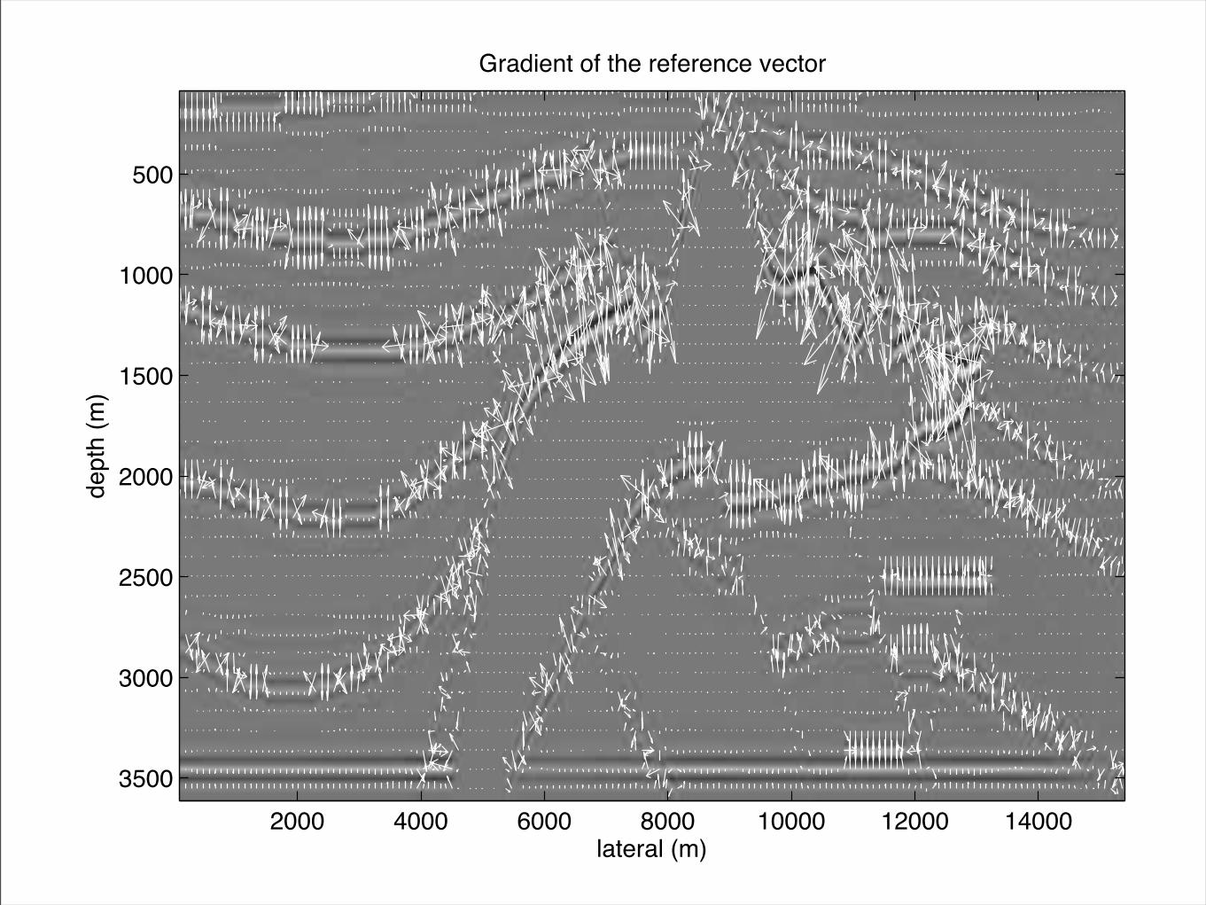
Gradient of the reference vector

lateral (m)

dept

h (m

)

2000 4000 6000 8000 10000 12000 14000

500

1000

1500

2000

2500

3000

3500

Step 1: Update of the Jacobian of 12!y "Ax!22:

x# x + AT (y "Ax) ;

Step 2: projection onto the !1 ball S = {!x!1 $ !x0!1} by soft thresholding

x# T!w(x);

Step 3: projection onto the anisotropic di!usion ball C = {x : J(x) $ J(x0)}by

x# x" "!xJc(x)

Recovery

Initialize:

m = 0;

x0 = 0;

y = KTd;

Choose:

M and L

!ATy!! > !1 > !2 > · · ·

while !y "A!x!2 > " do

m = m + 1;

xm = xm"1;

for l = 1 to L do

xm = T!m

"xm + AT (y " xm)

#{Iterative thresholding}

end for

Anisotropic descent update;

xm = xm " #!xm Jc(xm);

end while

!x = xm; !m ="AT

#† !x.

Table 2: Sparsity-and continuity-enhancing recovery of seismic amplitudes.

28

Application to the SEG AA’ model

ExampleSEGAA’ data:

“broad-band” half-integrated wavelet [5-60 Hz] 324 shots, 176 receivers, shot at 48 m 5 s of data

Modeling operator Reverse-time migration with optimal check pointing

(Symes ‘07) 8000 time steps linearized modeling 64, and migration 294 minutes

on 68 CPU’s

Scaling required 1 extra migration-demigration


Migrated data Amplitude-corrected & denoised migrated data


Noise-free data Noisy data(3 dB)

Data from migrated image

Data from amplitude-corrected & denoised migrated

image

ExampleSEGAA’ data:

“broad-band” half-integrated wavelet [5-60 Hz] 324 shots, 176 receivers, shot at 48 m 5 s of data

Modeling operator Reverse-time migration with optimal check pointing

(Symes ‘07) 8000 time steps full modeling

Scaling required 1 extra migration-demigration

ConclusionsCurvelet-domain scaling

handles conflicting dips (conormality assumption) exploits invariance under the PsDO robust w.r.t. noise

Diagonal approximation exploits smoothness of the symbol uses “neighbor” structure of the curvelet

transform

Results on the SEG AA’ show recovery of amplitudes beneath the Salt successful recovery of clutter improvement of the continuity

Acknowledgments

The authors of CurveLab (Demanet, Ying, Candes, Donoho)

Dr. W. W. Symes for his reverse-time migration code

This work was in part financially supported by the Natural Sciences and Engineering Research Council of Canada Discovery Grant (22R81254) and the Collaborative Research and Development Grant DNOISE (334810-05) of F.J.H. This research was carried out as part of the SINBAD project with support, secured through ITF (the Industry Technology Facilitator), from the following organizations: BG Group, BP, Chevron,ExxonMobil and Shell.

Stable seismic data recovery - University of British … · wavefronts & reflectors are multiscale...

Documents

Transcript of Stable seismic data recovery - University of British … · wavefronts & reflectors are multiscale...