Accepted for publication in J. Fluid Mech. 1

Stable Manifolds and the Transition toTurbulence in Pipe Flow

By 1D. VISWANATH AND 2P. CVITANOVI C1Department of Mathematics, University of Michigan, Ann Arbor, MI 48109, USA

2School of Physics, Georgia Institute of Technology, Atlanta, GA 30332, USA

(Received 27 October 2008)

Lower-branch traveling waves and equilibria computed in pipe flow and other shear flowsappear intermediate between turbulent and laminar motions. We take a step towardsconnecting these lower-branch solutions to transition by deriving a numerical methodfor finding certain special disturbances of the laminar flow in a short pipe. These specialdisturbances cause the disturbed velocity field to approach the lower-branch solution byevolving along its stable manifold. If the disturbance were slightly smaller, the flow wouldrelaminarize, and if slightly larger, it would transition to a turbulent state.

1. IntroductionThe connection between the law of resistance to water flowing in a tube and the sinuous

or direct nature of the internal motion of the fluid was established by Reynolds (1883). Inthe transitional regime, he observed “flashes” and recorded them in Figure 16 of his paper.Later experiments using hot-wire measurements have revealed the structure of puffs andslugs (Wygnanski and Champagne 1973). Particularly intriguing are equilibrium puffsthat maintain their spatial extent as they travel downstream with a characteristic speed(Wygnanski et al. 1975). Such puffs are approximately 20 pipe diameters long and areobserved for Re (Reynolds number) somewhat greater than 2000. Further, the structureof the puff is independent of the disturbance used to create it.

For a range of Re, the flow injected into the pipe assumes the familiar Hagen-Poiseuillelaminar profile downstream. The flow does not have the laminar profile at the inlet. There-fore it is important to distinguish between disturbances at the inlet and disturbances tofully developed laminar flow (Willis et al. 2008). The early experiments used inlet distur-bances, but in theoretical investigations such as this one, it has been common practiceto consider disturbances to the laminar flow.

In their experiments to determine the dependence of the threshold for transition onRe, Darbyshire and Mullin (1995) used a constant mass-flux pipe and introduced dis-turbances to the laminar flow at a point sufficiently downstream from the inlet. Theywere able to determine thresholds over a range of Re, but Figure 11 and other figures intheir paper showed that certain disturbances above the threshold do not transition whilecertain disturbances below the threshold do transition. Hof et al. (2003) determined thatthe threshold scaled as Reα with α = −1, when the laminar flow was disturbed by asingle boxcar pulse of fluid injected at six different points. Mellibovsky and Meseguer(2007) have reproduced α = −1 in a numerical study that added a body force term tothe Navier-Stokes equation to model the effect of the boxcar pulse of fluid. For differentdisturbances of the laminar flow, Peixinho and Mullin (2007) found α < −1. In thatexperiment, the transition is sequential, with flow visualizations showing the disturbance

2 D. Viswanath and P. Cvitanovic

changing its form as it travels downstream before leading to bigger structures. FollowingO’Sullivan and Breuer (1994), Peixinho and Mullin (2007) point out that disturbancesthat lead to α < −1 probably do not significantly distort the mean flow.

With regard to theory, Reynolds’s assertion that “there was small chance of discov-ering anything new or faulty” in the Navier-Stokes equation has stood the test of time.Thanks to numerical computations, we now know that the incompressible Navier-Stokesequation adequately explains a remarkable wealth of phenomena related to transitionalturbulence and fully developed turbulence. Although the Navier-Stokes equation can besolved numerically in certain regimes, the nature of the solutions of that equation hasproved difficult to understand.

It is clear, however, that the nature of the solutions is quite different in the turbulentand transitional regimes. Fully developed turbulence is characterized by rapid decay ofcorrelations and fine scales. Statistical theories that separate turbulent velocity fields intomeans and fluctuations have had significant successes (Narasimha 1989), even thoughcoherent motions are present in certain regions of fully developed turbulence (Robinson1991). In contrast, the transition problem seems to be fundamentally dynamical in nature.

Following the experiments of Darbyshire and Mullin (1995), Faisst and Eckhardt (2004)and Schmiegel and Eckhardt (1997) argued that there is no sharp boundary betweeninitial conditions that trigger turbulence and those that do not, and demonstrated com-putationally that the stability border for plane Couette flow is a fractal. One of theirsuggestions, namely that a chaotic saddle could be present for transitional Re, illustratesthe dynamical nature of the transition problem.

More recently, Faisst and Eckhardt (2003) and Wedin and Kerswell (2004) computed anumber of traveling wave solutions of pipe flow. Their work was preceded by computationsof somewhat similar solutions of channel flows by Nagata (1990) and Waleffe (1998).Hof et al. (2004) found streak patterns in puffs and slugs that appeared close to thoseof some pipe flow traveling waves. The traveling waves were computed in short pipes,typically only a few pipe diameters long, while puffs are as long as 20 pipe diameters.Therefore the following question may be asked: do the experimentally observed structurescorrespond to the computed traveling waves?

The correlation functions, such as those of Schneider et al. (2007a), used to detectstreak patterns in experimental or numerical flow fields look for m-fold rotational sym-metry with respect to the pipe axis. Using such a correlation function, Figure 5 ofSchneider et al. (2007a) illustrates a transition from a four streak state to a six streakstate within a spatial range of a single pipe radius. Willis and Kerswell (2008) foundstructures with m = 3 and m = 4 within streamwise distances of about 2 pipe diameterpreceding the trailing edge of the puff and 5 pipe diameters following the trailing edge.Figure 5 of their paper gives some evidence that parts of the puff on either side of itstrailing edge (but not at the trailing edge itself) visit traveling wave solutions with m = 3and m = 4. It could be significant that Figures 7 and 23 of Wedin and Kerswell (2004)(which use different units) imply that some of the m = 3 and m = 4 traveling waves havewave speeds relatively close to that of the puff. Willis and Kerswell (2008) also foundthat the qualitative comparisons of (Hof et al. 2004) which used slug cross-sections hadsignificant problems. Instead of the trailing edge of the puff, Eckhardt and Schneider(2008) used the center of turbulent energy to fix a position within a moving puff. Theircenter of turbulent energy is more precisely defined and it moves with the puff in a quiteregular manner. They found the axial correlation lengths around that center to be quiteshort. While the question raised in the previous paragraph cannot be answered conclu-sively at the moment, these arguments suggest that short pipe computations are of somerelevance.

Stable Manifolds and the Transition to Turbulence in Pipe Flow 3Re = 2000 Re = 4000

Figure 1. Contour plots of z-averaged streamwise velocity with the laminar flow subtracted.Rolls are superposed. The contour levels are equispaced in the intervals [−0.195, 0.170] and[−0.191, 0.148], respectively, with the lighter regions being faster. The maximum magnitude ofthe vectors in superposed quiver plots are 0.0075 and 0.0038, respectively.

Another point to be mentioned is that puffs, in which streak patterns resemblingthose of some traveling waves have been detected, are observed experimentally onlyfor Re < 2800. The transition experiments that measure thresholds (Hof et al. 2003;Peixinho and Mullin 2007) reach Re as high as 20000. Thus the relevance of puffs totransition may seem limited. However, there is a possibility that puffs exist as solutionsof the Navier-Stokes equation beyond the Re at which they are observed in experiments(Willis and Kerswell 2009).

Most of the lower branch solutions of pipe flow and the channel flows seem to be onthe laminar-turbulent boundary (Duguet et al. 2008; Gibson et al. 2008; Itano and Toh2001; Kawahara 2005; Kerswell 2005; Kerswell and Tutty 2007; Schneider et al. 2008;Viswanath 2008a; Wang et al. 2007), which means that for some tiny disturbances of thelower branch solution, the disturbed state evolves and becomes laminar uneventfully. Forother disturbances, the disturbed stated evolves and becomes turbulent, or undergoes aturbulent episode before it becomes laminar.

In this article, we investigate if there are small disturbances of the laminar solution,for which the disturbed state evolves and hits a given lower branch solution. By small,we mean firstly that the magnitude of the disturbance should decrease algebraically withRe and secondly that the disturbance should not change the mean flow significantly. Theexistence of such a disturbance would establish that the flow can transition from laminarto turbulence by passing through the vicinity of the given lower branch traveling wave.

In fact, Kreiss et al. (1994) found such disturbances when computing thresholds with-out fully realizing that they were hitting a lower branch equilibrium solution of planeCouette flow. But the situation they tackled is an especially simple one because the lowerbranch solution has a single unstable direction (Schneider et al. 2008; Toh and Itano2003; Viswanath 2008a; Wang et al. 2007). We consider the asymmetric traveling wavecomputed by Pringle and Kerswell (2007). That traveling wave has two unstable direc-tions both of which lie in a symmetric subspace, and thus serves to illustrate that themethod used for computing thresholds cannot be used to hit traveling waves that havemore than one unstable direction.

The asymmetric traveling wave of Pringle and Kerswell (2007), which has two faststreaks located near one side of the pipe, is shown in Figure 1. The preferential locationof the streaks towards one side is also found in edge states that occur in transition

4 D. Viswanath and P. Cvitanovic

Re I = D ke ked ke0 ke1 ke2 ke3

2000 1.0881 0.9783 0.013 0.9778 4.4e−4 2.3e−5 2.2e−72500 1.0802 0.9790 0.012 0.9788 2.8e−4 1.2e−5 1.0e−73000 1.0755 0.9794 0.012 0.9792 1.9e−4 7.6e−6 5.9e−84000 1.0705 0.9796 0.012 0.9795 1.1e−4 3.8e−6 2.8e−8

Table 1. The kinetic energy of the traveling wave and the kinetic energy with laminar flowsubtracted are denoted by ke and ked, respectively. The last four columns give the kinetic energyin modes with n = 0,±1,±2,±3.

computations (Schneider et al. 2007b). Table 1 gives basic data for that traveling waveat four different Re. That data will be useful for judging the closeness of approaches tothe traveling wave. The choice of units, the significance of I and D in Table 1, and themeaning of the streamwise modes with n = 0,±1,±2,±3 are explained in Section 2. Moreextensive data for the asymmetric traveling wave can be found elsewhere (Viswanath2008b).

To find a small disturbance of the laminar solution that evolves into a given lower-branch state, it is necessary to consider a linear superposition of disturbances whosedimension equals that of the unstable manifold of the lower-branch state. That require-ment follows from a consideration of the co-dimension of the stable manifold of thelower-branch state. In addition, the disturbances that are linearly combined must bechosen carefully.

To hit the asymmetric traveling wave, we consider three different disturbances of thelaminar solution. The first disturbance is obtained by extracting the rolls, which areformed by averaging the traveling wave in the streamwise direction and retaining onlythe radial and azimuthal components of the velocity field. The choice of rolls is relatedto the so-called lift-up mechanism (Landahl 1980). The two other disturbances are thetwo unstable eigenvectors of the traveling wave. If one of the eigenvectors is added to thetraveling wave, it has the effect of either reinforcing or weakening the fast streaks. Theother eigenvector seems to alter the location of the fast streaks. It must be remembered,however, that the disturbances are added to the laminar solution and not to the travelingwave.

In Section 4, we show that disturbances of the laminar flow obtained by varying anytwo of these three disturbances evolve and hit the traveling wave. The choice of theunstable eigenvectors might seem puzzling as our intention is to hit the traveling waveand not to move away from it. The reason that choice works is partially explained inSections 3 and 4. Section 4 also shows that the magnitudes of the disturbances neededto hit the asymmetric traveling wave diminish algebraically with Re.

All our computations use a pipe that is π pipe diameters long and the traveling wavesare computed with 85715 active degrees of freedom. The computations of relative periodicsolutions (or modulated traveling waves) in plane Couette flow use triple the number ofdegrees of freedom (Viswanath 2007), although those computations are roughly 5 to 10times as expensive with the same number of degrees of freedom. The computation oftraveling waves is an insignificant part of the total computational expense, however, aswill become clear in Section 4. We need to use a short pipe to keep the total computationalexpense manageable.

The pipe we use is too short to capture transitional structures such as puffs. To addto the earlier discussion of the relevance of short pipe computations of traveling waves,

Stable Manifolds and the Transition to Turbulence in Pipe Flow 5

we mention the work of Mellibovsky and Meseguer (2006) which seems to suggest thattransition scenarios can be independent of pipe length. The logic which is used to finddisturbances of the laminar solution that hit the asymmetric traveling wave makes fairlyintricate use of the dynamical properties of the traveling wave. More work is needed todetermine if the same logic is applicable to transition in pipes of more realistic length.

2. PreliminariesThe code for direct numerical simulation of pipe flow uses cylindrical coordinates with

u, v, and w being the components of the velocity in the radial (r), polar (θ), and axial (z)directions, respectively. The boundary conditions are no-slip at the walls and periodicin the z direction with constant mass-flux. The length of the periodic domain in thez direction is denoted by 2πΛ. We use Λ = 1 throughout. The units for distance andvelocity are chosen so that the pipe radius is 1 and the Hagen-Poiseuille profile is givenby w = 1− r2. The Reynolds number Re is based on the pipe radius, centerline velocityof the Hagen-Poiseuille flow, and kinematic viscosity ν. The unit of mass is chosen sothat the density of the fluid is 1. The units and boundary conditions follow those ofFaisst and Eckhardt (2004).

Let w(r) denote the mean velocity in the axial direction, and v(r) the mean velocityin the polar direction. The mass-flux per unit area is given by 2

∫ 1

0rw(r) dr and is equal

to 1/2 for all velocity fields that obey the boundary condition. The pressure gradientnecessary to maintain constant mass-flux varies from instant to instant. For the Hagen-Poiseuille flow, it is −4/Re.

The spatial discretization is spectral. The radial component of the velocity u is repre-sented as

u(r, θ, z) =n=N∑

n=−N

m=M∑m=−M

un,m(r) exp(imθ) exp(inz/Λ). (2.1)

For the velocity field to be regular at r = 0, the coefficients un,m(r) must be evenfunctions of r for odd m and odd functions of r for even m. Thus the functions canbe reconstructed by storing their values at r = cos(iπ/L), i = 0, 1, . . . , (L − 1)/2. Weassume L odd so that there is no point at r = 0 (Trefethen 2000). The radial componentof vorticity is denoted by ξ. It is represented in the same way u is represented. The otherquantities used to represent the velocity field are v(r), which is an odd function of r, andw(r) which is an even function of r. The velocity field is constructed using u, ξ, v, w andthe divergence free condition. The advection term was dealiased using the Orszag 3/2rule. All the computations use (N, M, L) = (16, 18, 81).

The rate of energy dissipation per unit mass is given by 2D/Re, where D is the integralof

14π2Λ

(1r2

(u2 + v2 − 2

∂u

∂θv + 2u

∂v

∂θ

)+

∑U=u,v,w

(∂U

∂r

)2

+(

∂U

∂z

)2

+1r2

(∂U

∂θ

)2)(2.2)

over the volume of the pipe. In its more familiar form, D is the integral of the sum ofthe norms of gradients of the three components of the velocity field (Wedin and Kerswell2004). The term under the summation in (2.2) gives |∇U |2 for a scalar field U(r, θ, z).The terms outside the summation in (2.2) arise as cross terms when that operator isapplied to u cos θ − v sin θ and u sin θ + v cos θ. The explicit form of (2.2) displays the1/r2 singularities that are hidden in vector notation. Because those singularities cancelat r = 0, the numerical evaluation of D in a spectral code is a delicate matter. The rate

6 D. Viswanath and P. Cvitanovic

of energy input per unit mass is given by 2I/Re, where

I = − Re

4π2Λ

∫∇ · (pu), (2.3)

with p being pressure and with the integral being over the volume of the pipe. For theHagen-Poiseuille laminar flow, both D and I evaluate to 1.

Figure 1 shows the asymmetric traveling wave solution first computed by Pringle and Kerswell(2007). To compute that traveling wave, we added rolls which approximate the pattern inFigure 1 to the laminar solution and evolved the velocity field to allow the streaks to de-velop. The resulting velocity field was used as the initial guess for the GMRES-hookstepmethod, which converged without a hitch. The number of active degrees of freedom inthe representation of a velocity field is (L − 2) + ((2N − 1)(2M − 1) − 1)(L − 3)/2. Themethod uses translation operators to handle the invariance of the pipe-flow equation withrespect to shifts along z and rotations along θ. These operators are given by

T1u(r, θ, z) =∑m,n

imun,m(r) exp(imθ) exp(inz/Λ)

T2u(r, θ, z) =∑m,n

(in/Λ)un,m(r) exp(imθ) exp(inz/Λ), (2.4)

where the indices m, n correspond to the representation (2.1). A detailed description ofthe GMRES-hookstep method can be found elsewhere (Viswanath 2007, 2008b).

The equations of pipe flow are unchanged by the shift-reflect symmetry:

u(r, θ, z) → u(r,−θ, z + πΛ)v(r, θ, z) → −v(r,−θ, z + πΛ)w(r, θ, z) → w(r,−θ, z + πΛ). (2.5)

The velocity field of the traveling wave of Figure 1 is also unchanged by this discretesymmetry.

The magnitudes of disturbances and the norms of velocity fields are given in Section 4and other places using the square root of kinetic energy norm. The kinetic energy, whichis reported in tables such as Table 1, is normalized to be 1 for laminar flow.

To conclude this section, we mention a technical point about pipe flow simulationusing spectral codes that appears not to have been discussed in the literature. Once theadvection term is computed, the equations for evolving the modes decouple for pairs(m, n) such that the resulting equations depend only upon r for a fixed (m, n). Thedecoupled equations will have terms with the factor m2/r2 + n2/Λ2 in the denominator,and because of that factor the terms will have a singularity at the point r = −imΛ/nin the complex plane. If the number 2N of grid points in the streamwise direction isincreased while keeping the pipe length 2πΛ fixed, that singularity moves closer to thereal line with greater values of n now being allowed. When the singularity moves closerto the real line, one has to use more grid points in the r direction to solve the decoupledequations with the same level of accuracy (Trefethen 2000).

3. Unstable manifold of the traveling waveTo find disturbances of the laminar solution that evolve and hit the asymmetric travel-

ing wave, it is essential to understand the unstable directions and the unstable manifoldof that traveling wave. Suppose we disturb the laminar solution using rolls of the ap-propriate form and some “noise”, the magnitude of which is a fixed fraction of that of

Stable Manifolds and the Transition to Turbulence in Pipe Flow 7

Re λ1 λ2 λ3

2000 0.03247 0.00897 −0.005942500 0.03049 0.00725 −0.02282 + i0.020413000 0.02861 0.00631 −0.01978 + i0.016644000 0.02529 0.00531 −0.01536 + i0.01190

Table 2. λ1 and λ2 are the only unstable eigenvalues. λ3 has the greatest real part amongthe stable eigenvalues whose eigenvectors lie in the shift-reflect invariant subspace.

−1 −0.5 0 0.5 1 1.5 2−1

−0.8

−0.6

−0.4

−0.2

0

0.2

0.4

0.6

0.8

1Re = 2000

−1 −0.5 0 0.5 1 1.5 2−1

−0.8

−0.6

−0.4

−0.2

0

0.2

0.4

0.6

0.8

1Re = 2500

Figure 2. For eigenvalues λ of the traveling wave, the plots show exp(10λ) as circles for easiervisualization. If the corresponding eigenvector lies in the shift-reflect invariant subspace, thecircle is solid.

the rolls, to introduce streamwise dependence. The disturbed state will evolve and de-velop streaks. At the point of closest approach to the traveling wave, we can think ofthe evolving velocity field as the traveling wave plus two components, one of which is acombination of the stable eigenvectors of the traveling wave with the other being a com-bination of the unstable eigenvectors. The stable eigenvectors will decay under evolution.However, the component along the unstable eigenvectors will be amplified and will takethe evolving velocity field away from the traveling wave. To ensure that the disturbedstate hits the traveling wave, the disturbance has to be arranged in such a way that theevolving velocity field is free of the unstable directions as it approaches the travelingwave.

Such a disturbance is easiest to arrange, if the traveling wave has only one unstabledirection. The component along that direction at the point of closest approach can beeliminated by simply varying the magnitude of the initial disturbance. However, theasymmetric traveling wave has two unstable directions as shown in Table 2. The twounstable eigenvalues λ1 and λ2 decrease with increasing Re at rates given by Re−0.41 andRe−0.87, respectively (Viswanath 2008b). Table 2 also shows the leading stable eigenvalue.

Figure 2 gives a more complete idea of the spectrum of the linearization around theasymmetric traveling wave. The spectra at different Re were computed using the Arnoldiiteration. Some of the interior eigenvalues near the centers of the circles in Figure 2 areomitted. But we are certain that no unstable eigenvalues are omitted. In addition, wehave verified that none of the eigenvalues in the figure is spurious.

Data for the unstable eigenvectors is given in Table 3. Most of the kinetic energy ofthe traveling waves themselves is in the n = 0 (or mean) mode, as shown in Table 1.Much of the kinetic energy remains in n = 0 for the λ1 eigenvector, although n = 1 now

8 D. Viswanath and P. Cvitanovic

λ1 λ2

Re ke0 ke1 ke2 ke3 ke0 ke1 ke2 ke2

2000 6.9e−1 2.6e−1 4.9e−2 1.1e−3 1.2e−1 7.4e−1 1.4e−1 3.1e−32500 7.0e−1 2.6e−1 4.2e−2 7.6e−4 1.1e−1 7.7e−1 1.2e−1 2.3e−33000 7.0e−1 2.6e−1 3.8e−2 6.2e−4 1.1e−1 7.8e−1 1.1e−1 1.9e−34000 7.0e−1 2.6e−1 3.2e−2 4.9e−4 1.1e−1 7.9e−1 9.4e−2 1.5e−3

Table 3. The kinetic energies in the n = 0,±1,±2,±3 modes of the λ1 and λ2 eigenvectors.The eigenvectors are normalized to have kinetic energy equal to 1.

λ1 mode λ

2 mode

Figure 3. Contour plots of the z-averaged streamwise velocity for the two unstable eigenvectorsat Re = 2500. If the eigenvectors are normalized to have unit kinetic energy, the level curvesare equispaced in the intervals [−1.38, 1.66] and [−1.01, 0.34], respectively. The lighter regionscorrespond to higher values. At other values of Re, the signs of the eigenvectors are chosen toyield plots similar to the ones above.

has more than a quarter of the kinetic energy. For the λ2 eigenvector, the n = 1 modedominates.

Figure 3 shows that the λ1 eigenvector weakens the high speed streaks of the travelingwave. The effect of adding the λ2 eigenvector to the traveling wave would be to displacethe high speed streaks to a more symmetrical position. It must be noted, however, thatthe plot of the streaks of the λ2 eigenvector is not as meaningful because the n = 1 modeis dominant. The two plots in Figure 3 are used to assign positive and negative signs tothe eigenvectors at different Re in a consistent manner. When comparing cross-sections ofvelocity fields to traveling wave solutions (Eckhardt and Schneider 2008; Hof et al. 2004;Willis and Kerswell 2008), it may be worthwhile to look at the unstable eigenvectors ofthe traveling waves. The inevitable deviations from the streak patterns of the travelingwaves may correlate with the streak patterns of the unstable eigenvectors.

Figure 4 shows the mean streamwise flow that corresponds to the λ1 and λ2 eigenvec-tors. To form an idea of the distortion to the mean flow of the laminar solution whenthose eigenvectors are added as disturbances, the plots in Figure 4 must be scaled by afactor of 1/50 or less.

Figure 5a shows that if the asymmetric traveling wave is disturbed with a small andpositive multiple of the λ1 eigenvector, the disturbed state evolves and becomes laminaruneventfully. That is unsurprising because the disturbance has the effect of weakening

Stable Manifolds and the Transition to Turbulence in Pipe Flow 9

0 0.2 0.4 0.6 0.8 1−0.3

−0.2

−0.1

0

0.1

0.2

0.3

0.4

0.5

0.6

λ1 mode

r

w

2000250030004000

0 0.2 0.4 0.6 0.8 1−0.3

−0.25

−0.2

−0.15

−0.1

−0.05

0

0.05

0.1

λ2 mode

r

w

2000250030004000

Figure 4. Plots of the mean streamwise flow w(r) at various values of Re. The eigenvectorsare normalized to have kinetic energy equal to 1.

(a)0 500 1000 1500

1

1.5

2

2.5

t

D o

r I

(b)0 100 200 300 400 500 600

1

1.5

2

2.5

t

D o

r I

Figure 5. (a) Plots of D (solid) and I (dashed) against time at Re = 2000 and Re = 2500. Forboth values of Re, perturbation of the traveling wave by a positive multiple of the λ1 eigenvectorshown in Figure 4 leads to rapid laminarization (thin lines at lower left corner). Perturbationby a negative multiple leads to a long transient at Re = 2000 and what appears to be sustainedturbulence at Re = 2500. (b) Plots close to the edge.

the high speed streaks. In contrast, adding a negative multiple leads to what appears tobe sustained turbulence at Re = 2500. It is easily noticeable that energy dissipation D isgreater than energy input I when the plots in Figure 5a spike up, but is lesser when theplots dip down. Thus the kinetic energy of the velocity field as a whole decreases during

10 D. Viswanath and P. Cvitanovic

(a)

v1

v2

(b)

−0.15 −0.1 −0.05 0 0.05 0.1−0.01

0

0.01

0.02

0.03

0.04

0.05

c1

c 2

Figure 6. (a) A schematic sketch of directions on the unstable manifold, where the two eigenvec-tors are labeled. The trajectories initiated in the dashed directions undergo turbulent episodes.(b) Projections of trajectories whose initial points are obtained by perturbing the traveling waveat Re = 2500 by a combination of the λ1 and λ2 modes. The initial points are all near (0, 0).The trajectories that laminarize turn right, while those that transition to turbulence (dashed)turn left.

the spikes, but increases during the dips. The decrease of kinetic energy during a spikeis well correlated with flattening of the mean velocity profile.

Figure 6a shows a schematic sketch of the unstable directions of the asymmetric trav-eling wave, while distinguishing between directions that turn turbulent and ones that donot. Figure 5b corresponds to two trajectories close to the border between turbulent andlaminar directions. In that figure, the trajectories near the border separate after t = 300.By refining the border, it appears that the point of separation can be deferred indefinitelywith a view to locating edge states.

To better visualize the unstable manifold, we adopt a technique introduced by Gibson et al.(2008) with the aim of getting good phase space visualizations of turbulent trajectories.The velocity field is a point in phase space and the evolution of an initial velocity fieldwith respect to the incompressible Navier-Stokes equation is a trajectory in that phasespace. Because the phase space is infinite-dimensional and does not lend itself to plotsdirectly, one has to use projections. An obvious projection would be to pick some Fourier-Chebyshev modes from the discretization of the velocity field. Although such projectionshave been employed, they have a number of shortcomings. The choices of the componentof the velocity vector and of the mode of that component are both arbitrary. The com-ponent and the mode that are chosen capture only a partial aspect of the velocity field.As a result of these shortcomings, such projections look messy and one cannot form agood idea of the dynamical structures in phase space from such projections.

Following (Gibson et al. 2008), the projection we use picks a set of velocity fieldsthat appears well suited to visualize trajectories on the unstable manifold. Let uTW

be the velocity field of the traveling wave and let u′ and u′′ be an orthonormal basisfor its unstable space. The notion of orthogonality between velocity fields correspondsto the kinetic energy norm. We will choose u′ to be the same direction as the leadingeigenvector. With that choice the second eigenvector at Re = 2500 is approximately−0.13u′ + 0.99u′′. For each velocity field that satisfies the shift-reflect symmetry (2.5),we obtain a projection in terms of uTW , u′, and u′′. The velocity fields u′ and u′′ satisfythe no-slip boundary condition and have zero mass-flux.

Stable Manifolds and the Transition to Turbulence in Pipe Flow 11

fr f1 f2 T δ ke0 ke1 ke2 ke3

7.084220e−3 −2.114944e−2 0 371.49 8.1e−4 9.8e−1 4.3e−4 2.2e−5 2.1e−71.242439e−2 1.890000e−2 0 219.70 8.9e−3 9.8e−1 3.3e−4 1.4e−5 1.0e−79.119378e−3 0 1.720663e−2 257.80 4.2e−3 9.8e−1 4.1e−4 2.0e−5 1.9e−71.017473e−2 0 −1.400000e−2 240.90 5.5e−3 9.8e−1 3.7e−4 1.7e−5 1.4e−79.048182e−3 3.923814e−4 1.757170e−2 281.40 2.9e−3 9.8e−1 4.2e−4 2.2e−5 2.0e−7

5.687034e−3 −1.643322e−2 0 323.84 2.9e−3 9.8e−1 2.5e−4 1.0e−5 7.7e−89.591329e−3 1.562075e−2 0 318.60 7.7e−3 9.8e−1 3.1e−4 1.5e−5 1.4e−77.049209e−3 0 1.420195e−2 268.00 4.8e−3 9.8e−1 2.4e−4 9.4e−6 6.9e−87.986395e−3 0 −1.115761e−2 309.80 6.0e−3 9.8e−1 2.2e−4 8.1e−6 5.5e−85.676511e−3 −1.646355e−2 8.768074e−5 292.70 3.7e−3 9.8e−1 2.9e−4 1.3e−5 1.2e−7

Table 4. Data at Re = 2000 (above the double line) and at Re = 2500 (below the doubleline). The fs are magnitudes of disturbances of the laminar solution. T is the time of closestapproach to the traveling wave. δ is the distance from the traveling wave at that time. The lastfour columns give the kinetic energies in the n = 0,±1,±2,±3 modes at the point of closestapproach.

Given a velocity field u that satisfies the shift-reflect symmetry, one can decomposeit as u − uTW = c0u′ + c1u′′ + r, where the remainder r is orthogonal to the plane ofthe eigenvectors. One could use c0 and c1 to represent u in a plot, but that would beunsatisfactory. The problem is that one can translate uTW in the streamwise directionand obtain different velocity fields that stand for the same wave. In order to eliminatedependence on translations in the z direction, we shift the velocity field u by sz in the zdirection and consider

u(r, θ, z + sz) − uTW = c0u′ + c1u′′ + rsz . (3.1)

The shift sz is chosen to minimize ‖rsz‖, and the axes of the projection, c0 and c1, arethe coefficients for that shift. The need to pick a shift sz arises because the equationsof pipe-flow are unchanged by translations along z. The shift-reflect symmetry is brokenby rotations in the θ direction. Since we have restricted ourselves to vector fields withthe shift-reflect symmetry, shifts in θ are not considered in (3.1). The need to factor outcontinuous symmetries arises in ODEs (Gilmore and Letellier 2007) and PDEs such asthe Kuramoto-Sivashinky equation as well (Cvitanovic et al. 2007).

Figure 6b shows trajectories on the unstable manifold using such a projection. Theinitial velocity fields were of the form uTW + εau′ + εbu′′, with ε = ×10−4 and a, b beingscalars. In all, we considered ten velocity fields corresponding to (a, b) = (±1,±1), thefour coordinate directions, and two directions along the second eigenvector. Since ε issmall, all these velocity fields were very nearly on the unstable manifold. The distinctionbetween trajectories that laminarize uneventfully and those that undergo a turbulentepisode is clear in Figure 6b.

In the next section, we return to such projections of the unstable manifold to partiallyjustify arguments used to find disturbances of the laminar flow which evolve and hit theasymmetric traveling wave.

4. Hitting the traveling wave at Re = 2000 and Re = 2500The fr column of Table 4 gives the norm of the rolls. The velocity field of the rolls,

denoted by ur, is obtained by averaging the traveling wave in the streamwise directionand discarding the streamwise component of the velocity. The norms of the unstable

12 D. Viswanath and P. Cvitanovic

eigenvectors are denoted by f1 and f2. The velocity fields of the eigenvectors are denotedby u1 and u2. The laminar solution is uL and the traveling wave is uTW .

The distance δ of closest approach listed in Table 4 is obtained as follows. The Navier-Stokes equation is integrated from the initial velocity field uL + frur + f1u1 + f2u2.The initial velocity field has the shift-reflect symmetry and so does ut, where ut is thevelocity field at time t. Define

δ(fr, f1, f2) = mint≥0

min0≤sz<2πΛ

‖ut(r, θ, z + sz) − uTW ‖. (4.1)

To compare ut and uTW , one has to minimize over shifts sz for the same reason as in(3.1). To find the minimizing shift sz, we first try sz = πΛk/N , 0 ≤ k < 2N . Usingthat data, an interval that contains the minimum is found and that interval is refinedrecursively to a depth equal to 30. We refer to the result of the inner minimum in (4.1)as the distance between uTW and ut. This method of finding that distance is expensive,with the cost of finding the distance being more than 20 times the cost of a single timestep. However, it finds the distance with an accuracy of 4 or 5 digits.

Given the expense of finding the distance between ut and uTW , the distance being theinner minimum in (4.1), care has to be exercised in finding the outer minimum over t.If the distance is computed after every time step, the cost of the computation becomesprohibitive. The wall time for integrating a velocity field for a time interval of 100 isabout an hour on an Opteron processor, but becomes more than 20 hours if the distanceto uTW is computed after every time step. For an initial waiting time when the streaksare still forming, we do not compute the distance at all. This waiting time is longer forlarger Re. Thereafter the distance is computed every 100 time steps only, a time stepbeing 0.01. As the distances vary smoothly as a function of time, we use polynomialextrapolation to predict if the distance function has a minimum within the next 100time steps or not. If it is predicted to have a minimum within the next 100 time steps,we measure the distance every 10 time steps. If the distance function is predicted to havea minimum within the next 10 time steps, we measure the distance after every time step.The value of δ is the first local minimum found in this manner and it is very probablyalso the global minimum over t. The time step can be successively decreased to get finerestimates of δ, but that was not implemented.

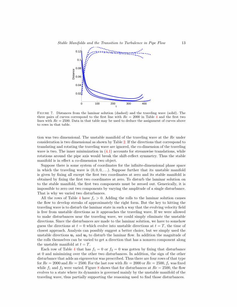
The times T at which the minima were attained are given in Table 4. T is measuredwith a precision of .01 in only two lines of that table. The measurements in the other lineshave a precision of 0.1. If the last four columns of that table are compared with the lastfour columns of Table 1, the comparison confirms that the approach to the traveling waveis closer when δ is smaller. Figure 7 leaves no room for doubt that the first disturbanceslisted for Re = 2000 and Re = 2500 in Table 4 evolve and hit the corresponding travelingwaves. The smallest distance δ from the traveling wave is realized after time T , which islisted in Table 4. Figure 7 shows that the plots of the distances from the traveling waveand the laminar solution both become flat around t = T . The disturbance moves awayfrom the laminar solution rapidly at t = 0. In contrast, for heteroclinic connections thereare two flat regions in t, which correspond to time spent in the neighborhoods of theinvariant solutions joined by the heteroclinic connection (Halcrow et al. 2008).

We are yet to explain the method used to find the numbers fr, f1, and f2 in Table 4.With each of those disturbances to the laminar solution, the disturbed state lands closeto the stable manifold of the traveling wave and evolves to make a close approach ofsmall δ to the traveling wave. Each line Table 4 was obtained by minimizing δ(fr, f1, f2)in different ways. The manner of minimization will now be described.

Although δ has three arguments corresponding to three disturbances, each minimiza-

Stable Manifolds and the Transition to Turbulence in Pipe Flow 13

0 100 200 300 400

0.02

0.04

0.06

0.08

0.1

0.12

Dis

tanc

e

t

Figure 7. Distances from the laminar solution (dashed) and the traveling wave (solid). Thethree pairs of curves correspond to the first line with Re = 2000 in Table 4 and the first twolines with Re = 2500. Data in that table may be used to deduce the assignment of curves aboveto rows in that table.

tion was two dimensional. The unstable manifold of the traveling wave at the Re underconsideration is two dimensional as shown by Table 2. If the directions that correspond totranslating and rotating the traveling wave are ignored, the co-dimension of the travelingwave is two. The inner minimization in (4.1) accounts for streamwise translations, whilerotations around the pipe axis would break the shift-reflect symmetry. Thus the stablemanifold is in effect a co-dimension two object.

Suppose there is some system of coordinates for the infinite-dimensional phase spacein which the traveling wave is (0, 0, 0, . . .). Suppose further that its unstable manifoldis given by fixing all except the first two coordinates at zero and its stable manifold isobtained by fixing the first two coordinates at zero. To disturb the laminar solution onto the stable manifold, the first two components must be zeroed out. Generically, it isimpossible to zero out two components by varying the amplitude of a single disturbance.That is why we varied two disturbances.

All the rows of Table 4 have fr > 0. Adding the rolls to the laminar solution causesthe flow to develop streaks of approximately the right form. But the key to hitting thetraveling wave is to disturb the laminar state in such a way that the evolving velocity fieldis free from unstable directions as it approaches the traveling wave. If we were allowedto make disturbances near the traveling wave, we could simply eliminate the unstabledirections. Since the disturbances are made to the laminar solution, we have to somehowguess the directions at t = 0 which evolve into unstable directions at t = T , the time ofclosest approach. Analysis can possibly suggest a better choice, but we simply used theunstable directions u1 and u2 to disturb the laminar flow. In addition the magnitude ofthe rolls themselves can be varied to get a direction that has a nonzero component alongthe unstable manifold at t = T .

Each row of Table 4 that has f1 = 0 or f2 = 0 was gotten by fixing that disturbanceat 0 and minimizing over the other two disturbances. In addition, the sign of the otherdisturbance that adds an eigenvector was prescribed. Thus there are four rows of that typefor Re = 2000 and Re = 2500. For the last row with Re = 2000 or Re = 2500, fr was fixedwhile f1 and f2 were varied. Figure 8 shows that for disturbances at Re = 2500, the flowevolves to a state where its dynamics is governed mainly by the unstable manifold of thetraveling wave, thus partially supporting the reasoning used to find those disturbances.

14 D. Viswanath and P. Cvitanovic

−0.1 −0.05 0 0.05 0.1−0.01

0

0.01

0.02

0.03

0.04

0.05

c1

c 2

Figure 8. Similar to Figure 6a, but the thick lines show the projections of trajectories atRe = 2500 which are initialized using the disturbances in Table 4.

101

102

103

10−4

10−3

10−2

10−1

Time

Dis

tanc

e

Figure 9. The axes correspond to the T and δ columns in Table 4. The plot is for Re = 2500.Each point corresponds to a certain stage in the sequence of optimizations used to find a dis-turbance of the laminar flow such that the disturbed flow evolves and hits the traveling wave.

When δ(fr, f1, f2) is minimized numerically, the disturbances found at successive stagesof the minimization give smaller δ but with larger values of T , the time of closest approachto the traveling wave, as shown in Figure 9. For the theoretical ideal δ = 0, T would beinfinite. Thus the numerical optimization becomes progressively more expensive.

A more severe impediment to numerical minimization is the non-smooth dependenceof δ on the disturbances when δ = 0. Because the time to hit the traveling wave diverges,even a small change in the disturbances causes a big change in the value of δ.

The numerical optimization was implemented using Matlab’s fmincon(), which allowsconstraints to be placed on the values of fr or f1 or f2. The C++ code for computing thefunction δ(fr, f1, f2) was invoked from Matlab. The unconstrained version fminunc()was not used because it tends to take such large steps while varying fr or f1 or f2 thatthe numerical integration of the Navier-Stokes equation becomes unstable. Because of thenon-smoothness, a nonlinear least squares solver, such as Matlab’s lsqnonlin(), might bea better option than fmincon(). lsqnonlin() minimizes

√|x + 2| from x = 3 with just

6 function evaluations while fmincon() takes 63 function evaluations to find a slightly

Stable Manifolds and the Transition to Turbulence in Pipe Flow 15

Re fr f1 f2 T δ ke0 ke1 ke2 ke3

2000 9.119378e−3 0 1.720663e−2 257.80 4.2e−3 9.8e−1 4.1e−4 2.0e−5 1.9e−72500 7.049209e−3 0 1.420195e−2 268.00 4.8e−3 9.8e−1 2.4e−4 9.4e−6 6.9e−83000 6.466047e−3 0 −9.890996e−3 356.61 7.0e−3 9.8e−1 2.2e−4 9.4e−6 8.4e−84000 4.600000e−3 0 8.829559e−3 386.95 9.5e−3 9.8e−1 6.9e−5 1.5e−6 7.1e−9

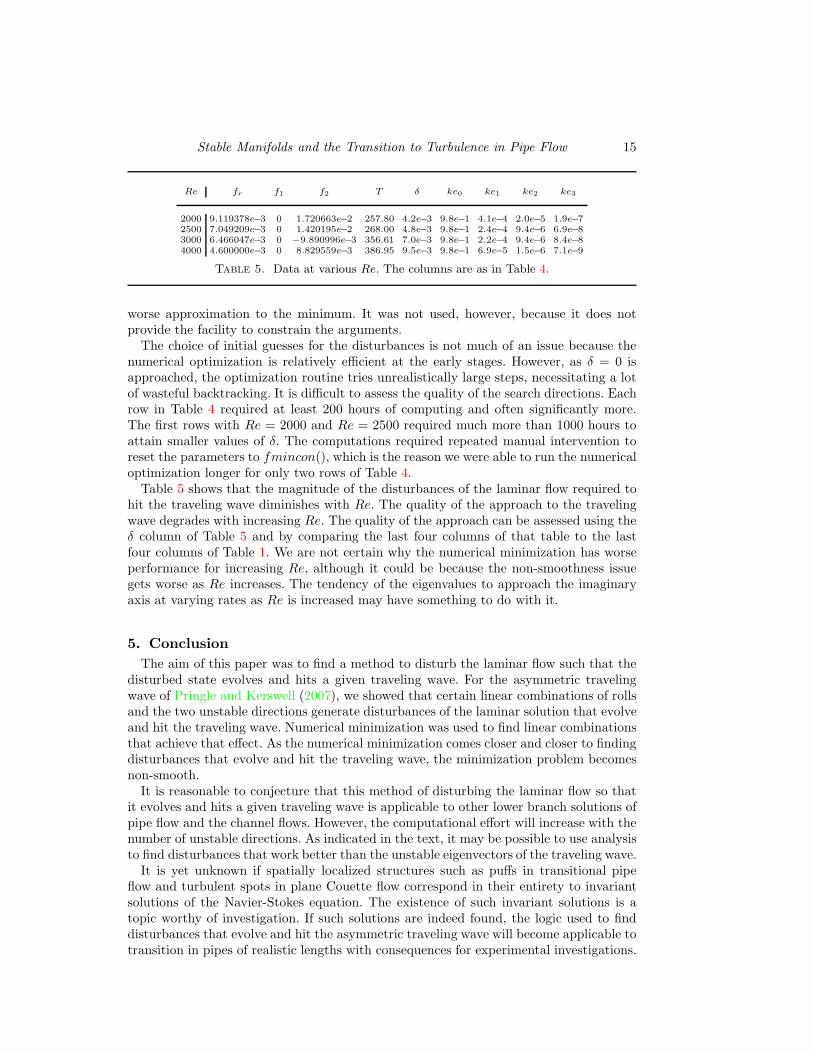
Table 5. Data at various Re. The columns are as in Table 4.

worse approximation to the minimum. It was not used, however, because it does notprovide the facility to constrain the arguments.

The choice of initial guesses for the disturbances is not much of an issue because thenumerical optimization is relatively efficient at the early stages. However, as δ = 0 isapproached, the optimization routine tries unrealistically large steps, necessitating a lotof wasteful backtracking. It is difficult to assess the quality of the search directions. Eachrow in Table 4 required at least 200 hours of computing and often significantly more.The first rows with Re = 2000 and Re = 2500 required much more than 1000 hours toattain smaller values of δ. The computations required repeated manual intervention toreset the parameters to fmincon(), which is the reason we were able to run the numericaloptimization longer for only two rows of Table 4.

Table 5 shows that the magnitude of the disturbances of the laminar flow required tohit the traveling wave diminishes with Re. The quality of the approach to the travelingwave degrades with increasing Re. The quality of the approach can be assessed using theδ column of Table 5 and by comparing the last four columns of that table to the lastfour columns of Table 1. We are not certain why the numerical minimization has worseperformance for increasing Re, although it could be because the non-smoothness issuegets worse as Re increases. The tendency of the eigenvalues to approach the imaginaryaxis at varying rates as Re is increased may have something to do with it.

5. ConclusionThe aim of this paper was to find a method to disturb the laminar flow such that the

disturbed state evolves and hits a given traveling wave. For the asymmetric travelingwave of Pringle and Kerswell (2007), we showed that certain linear combinations of rollsand the two unstable directions generate disturbances of the laminar solution that evolveand hit the traveling wave. Numerical minimization was used to find linear combinationsthat achieve that effect. As the numerical minimization comes closer and closer to findingdisturbances that evolve and hit the traveling wave, the minimization problem becomesnon-smooth.

It is reasonable to conjecture that this method of disturbing the laminar flow so thatit evolves and hits a given traveling wave is applicable to other lower branch solutions ofpipe flow and the channel flows. However, the computational effort will increase with thenumber of unstable directions. As indicated in the text, it may be possible to use analysisto find disturbances that work better than the unstable eigenvectors of the traveling wave.

It is yet unknown if spatially localized structures such as puffs in transitional pipeflow and turbulent spots in plane Couette flow correspond in their entirety to invariantsolutions of the Navier-Stokes equation. The existence of such invariant solutions is atopic worthy of investigation. If such solutions are indeed found, the logic used to finddisturbances that evolve and hit the asymmetric traveling wave will become applicable totransition in pipes of realistic lengths with consequences for experimental investigations.

16 D. Viswanath and P. Cvitanovic

Acknowledgments. The authors thank J.F. Gibson and the referees for helpful dis-cussions. The Center for Advanced Computing at the University of Michigan providedcomputing facilities. DV was partly supported by NSF grants DMS-0407110 and DMS-0715510. PC was partly supported by NSF grant DMS-0807574.

REFERENCES

P. Cvitanovic, R.L. Davidchack, and E. Siminos. State space geometry of a spatio-temporallychaotic Kuramoto-Sivashinsky flow. 2007. Available at arXiv:0709.2944.

A.G. Darbyshire and T. Mullin. Transition to turbulence in constant-mass-flux pipe flow. Journalof Fluid Mechanics, 289:83–114, 1995.

Y. Duguet, A.P. Willis, and R.R. Kerswell. Transition in pipe flow: the saddle structure onthe boundary of turbulence. Journal of Fluid Mechanics, 613:255–274, 2008. Available atarXiv:0711.2175.

B. Eckhardt and T. Schneider. How does flow in a pipe become turbulent? European PhysicalJournal B, 64:457–462, 2008.

H. Faisst and B. Eckhardt. Sensitive dependence on initial conditions in transition to turbulencein pipe flow. Journal of Fluid Mechanics, 504:343–352, 2004.

H. Faisst and B. Eckhardt. Traveling waves in pipe flow. Physical Review Letters, 91:224502,2003.

J.F. Gibson, J. Halcrow, and P. Cvitanovic. Visualizing the geometry of state space in plane Cou-ette flow. Journal of Fluid Mechanics, 611:107–130, 2008. Available at arXiv:0705.3957.

R. Gilmore and C. Letellier. The Symmetry of Chaos. Oxford University Press, Oxford, 2007.J. Halcrow, J. F. Gibson, P. Cvitanovic, and D. Viswanath. Heteroclinic connections in plane

Couette flow. Available at arXiv:0808.1865., 2008.B. Hof, A. Juel, and T. Mullin. Scaling of the turbulence transition threshold in a pipe. Physical

Review Letters, 91:244502, 2003.B. Hof, C.W.H. van Doorne, et al. Experimental observation of nonlinear traveling waves in

turbulent pipe flows. Science, 305:1594–1598, 2004.T. Itano and S. Toh. The dynamics of bursting process in wall turbulence. Journal of the

Physical Society of Japan, 70:701–714, 2001.G. Kawahara. Laminarization of minimal plane Couette flow: going beyond the basin of attrac-

tion of turbulence. Physics of Fluids, 17:041702, 2005.R.R. Kerswell. Recent progress in understanding the transition to turbulence in a pipe. Non-

linearity, 18:R17–R44, 2005.R.R. Kerswell and O.R. Tutty. Recurrence of travelling waves in transitional pipe flow. Journal

of Fluid Mechanics, 584:69–102, 2007.G. Kreiss, A. Lundbladh, and D.S. Henningson. Bounds for threshold amplitudes in subcritical

shear flows. Journal of Fluid Mechanics, 270:175–198, 1994.M.T. Landahl. A note on an algebraic instablity of inviscid parallel shear flows. J. Fluid Mech.,

98:243–251, 1980.F. Mellibovsky and A. Meseguer. The role of streamwise perturbations in pipe flow transition.

Physics of Fluids, 18:074104, 2006.F. Mellibovsky and A. Meseguer. Pipe flow transition threshold following localized impulsive

perturbations. Physics of Fluids, 19:044102, 2007.M. Nagata. Three dimensional finite amplitude solutions in plane Couette flow: bifurcation from

infinity. Journal of Fluid Mechanics, 217:519–527, 1990.R. Narasimha. The utility and drawbacks of traditional approaches. In J. Lumley, editor,

Whither Turbulence? Turbulence at the Cross-Road, pages 13–48. Springer-Verlag, Berlin,1989.

P.L. O’Sullivan and K.S. Breuer. Transient growth in circular pipe flow ii. Physics of Fluids, 6:3652–3664, 1994.

J. Peixinho and T. Mullin. Finite-amplitude thresholds for transition in pipe flow. Journal ofFluid Mechanics, 582:169–178, 2007.

C.C.T. Pringle and R.R. Kerswell. Asymmetric, helical, and mirror-symmetric traveling wavesin pipe flow. Physical Review Letters, 99:074502, 2007.

Stable Manifolds and the Transition to Turbulence in Pipe Flow 17

O. Reynolds. An experimental investigation of the circumstances which determine whether themotion of water shall be direct or sinuous, and of the law of resistance in parallel channels.Philosophical Transactions of the Royal Society of London, 174:935–982, 1883.

S.K. Robinson. Coherent motions in the turbulent boundary layer. Annual Review of FluidMechanics, 23:601–639, 1991.

A. Schmiegel and B. Eckhardt. Fractal stability border in plane Couette flow. Physical ReviewLetters, 79:5250, 1997.

T.M. Schneider, B. Eckhardt, and J. Vollmer. Statistical analysis of coherent structures intransitional pipe flow. Physical Review E, 75:066313, 2007a.

T.M. Schneider, B. Eckhardt, and J.A. Yorke. Turbulence transition and edge of chaos in pipeflow. Physical Review Letters, 99:034502, 2007b.

T.M. Schneider, J.F. Gibson, M. Lagha, F. De Lillo, and B. Eckhardt. Laminar-turbulentboundary in plane Couette flow. Physical Review E, 78:037301, 2008. Available atarXiv:0805.1015.

S. Toh and T. Itano. A periodic-like solution in channel flow. Journal of Fluid Mechanics, 481:67–76, 2003.

L.N. Trefethen. Spectral Methods in Matlab. SIAM, Philadelphia, 2000.D. Viswanath. Recurrent motions within plane Couette turbulence. Journal of Fluid Mechanics,

580:339–358, 2007.D. Viswanath. The dynamics of transition to turbulence in plane Couette flow. In Mathematics

and Computation, a Contemporary View. The Abel Symposium 2006, volume 3 of AbelSymposia. Springer-Verlag, Berlin, 2008a. Available at arXiv:0701337.

D. Viswanath. The critical layer in pipe flow at high Re. Philosophical Transactions of theRoyal Society A, 2008b. To appear.

F. Waleffe. Three-dimensional coherent states in plane shear flows. Physical Review Letters, 81:4140–4143, 1998.

J. Wang, J.F. Gibson, and F Waleffe. Lower branch coherent states in shear flows: transitionand control. Physical Review Letters, 98:204501, 2007.

H. Wedin and R.R. Kerswell. Exact coherent structures in pipe flow: travelling wave solutions.Journal of Fluid Mechanics, 508:333–371, 2004.

A.P. Willis and R.R. Kerswell. Coherent structures in localised and global pipe turbulence.Physical Review Letters, 100:124501, 2008.

A.P. Willis and R.R. Kerswell. Turbulent dynamics of pipe flow captured in a reduced model: puffrelaminarisation and localised ‘edge’ states. Journal of Fluid Mechanics, 2009. Availableat arXiv:0712.2739.

A.P. Willis, J. Peixinho, R.R. Kerswell, and T. Mullin. Experimental and theoretical progressin pipe flow transition. Philosophical Transactions of the Royal Society A, 366:2671–2684,2008.

I. Wygnanski, M. Sokolov, and D. Friedman. On transition in a pipe. Part 2. The equilibriumpuff. Journal of Fluid Mechanics, 69:283–304, 1975.

I.J. Wygnanski and F.H. Champagne. On transition in a pipe. Part 1. The origin of puffs andslugs and the flow in a turbulent slug. Journal of Fluid Mechanics, 59:281–335, 1973.