Stabilizers and Simulating Entanglement

Mark Howard(National University of Ireland, Maynooth)

CBSSS - Summer 2004e-mail: mhoward@thphys.may.ie

Abstract

The boundary between classical information and quantum infor-mation is investigated. More specifically, the stabilizer formalism andthe simulation of entangled states are considered. It is shown thatBell state correlations arising from measurements from the Pauli groupcan be simulated using local hidden variables. An explicit protocol forsimulating GHZ state correlations using local hidden variables and twoclassical bits of communication is derived.

1 Introduction

Historically, fundamental physics was originally concerned with matter -what it was and how it moved. Later the emphasis switched to energy andhow it was transformed and expressed. We know now that there can be nosuch thing as information without its physical representation, be it encodedas ink on a page, as 1’s and 0’s in a digital computer or as qubits in aquantum mechanical system. In short: information is physical. As moreis learned it seems reasonable to wonder if physics is informational - if aninformation-theoretical framework is more fruitful in terms of generatingnew laws and principles.

Classical information theory is now seen to be part of the more generaltheory of quantum information. The building block of Q.I.T. is the qubit.Qubits have the states |0〉 and |1〉 corresponding to the classical 0 and 1 but

1

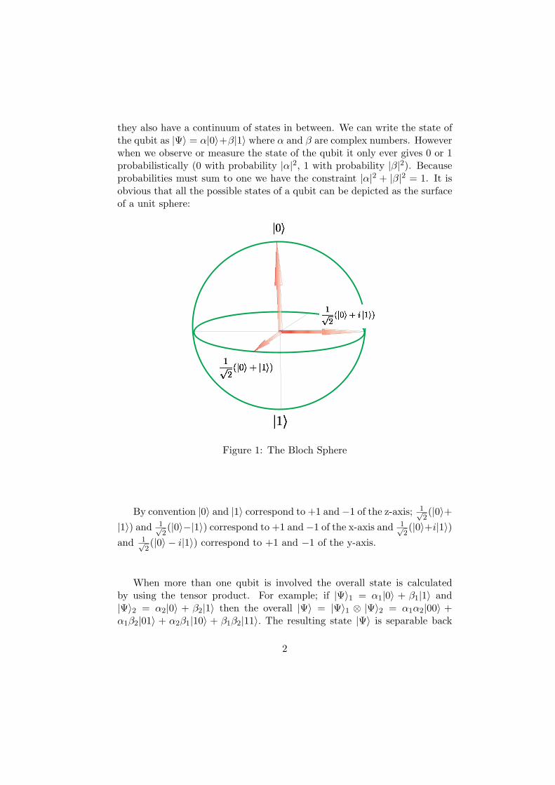
they also have a continuum of states in between. We can write the state ofthe qubit as |Ψ〉 = α|0〉+β|1〉 where α and β are complex numbers. Howeverwhen we observe or measure the state of the qubit it only ever gives 0 or 1probabilistically (0 with probability |α|2, 1 with probability |β|2). Becauseprobabilities must sum to one we have the constraint |α|2 + |β|2 = 1. It isobvious that all the possible states of a qubit can be depicted as the surfaceof a unit sphere:

Figure 1: The Bloch Sphere

By convention |0〉 and |1〉 correspond to +1 and−1 of the z-axis; 1√2(|0〉+

|1〉) and 1√2(|0〉−|1〉) correspond to +1 and−1 of the x-axis and 1√

2(|0〉+i|1〉)

and 1√2(|0〉 − i|1〉) correspond to +1 and −1 of the y-axis.

When more than one qubit is involved the overall state is calculatedby using the tensor product. For example; if |Ψ〉1 = α1|0〉 + β1|1〉 and|Ψ〉2 = α2|0〉 + β2|1〉 then the overall |Ψ〉 = |Ψ〉1 ⊗ |Ψ〉2 = α1α2|00〉 +α1β2|01〉 + α2β1|10〉 + β1β2|11〉. The resulting state |Ψ〉 is separable back

2

into two one-qubit states. Because of the very many degrees of freedom inthe quantum mechanical arena (Hilbert space) the majority of states arenon-separable or entangled e.g.

1√2(|00〉+ |11〉).

This is a Bell state. When the first qubit is measured it will return ananswer of either 0 or 1 with equal probability and will also collapse the wavefunction to |00〉 or |11〉 respectively. A measurement of the second qubitalways gives the same result as the measurement of the first qubit. In factthe measurement correlations of a Bell state are stronger thancould ever exist between classical systems.

It is interesting to examine situations where classical and quantum in-formation can be compared quantitatively. In the case of superdense codingtwo classical bits of information can be sent for the cost of measuring a(2-qubit) Bell state shared between Alice and Bob. Using teleportation one(possibly unknown) qubit can be sent from Alice to Bob for the cost of twoclassical bits of information and a shared (2-qubit) Bell state.

Results like Shor’s factoring algorithm and the Deutsch-Jozsa algorithmclearly show that important and exploitable differences exist between quan-tum and classical information. The stabilizer formalism, however, and theKnill-Gottesmann theorem which results from it depict the surprisingly largeextent to which quantum evolution and measurement can be efficiently sim-ulated on a classical computer. This is the subject of Section 2.

It has been shown experimentally that nature is not locally realistic i.e.that either one or both of the classical assumptions of locality (a measure-ment here will not affect a measurement elsewhere) and realism (that phys-ical properties have definite values independent of observation) are wrong.John Bell predicted this by showing that quantum correlations can violatean inequality which encapsulates the maximum allowable correlation by alocally realistic theory. The violation, therefore, of a Bell inequality indi-cates that something intrinsically quantum is going on. In order to quantify

3

just how much, one can ask the question: “ What classical resources arerequired to achieve the same correlations as this quantum state ? ”. Thisquestion is answered for two specific cases in Section 3.

2 Stabilizer Formalism

The stabilizer formalism allows for an unusual but often very compact wayof representing quantum states and processes.

Stabilizer : An operator O stabilizes the state |ψ〉 if O|ψ〉 = |ψ〉.

Group theory: A group is a set G (with elements gi ) in addition toan operation • which together satisfy certain properies like closure.

The Pauli Group on one qubit is the set { ±1, ±i, X, Y , Z} combinedwith the operation Matrix Multiplication where

X = σx =(

0 11 0

), Y = σy =

(0 −ii 0

), Z = σz =

(1 00 −1

).

X2 = Y 2 = Z2 = I

Y = iXZ.

The Pauli group on n qubits is the set containing all the different possibletensor product combinations of n Pauli operators e.g for two qubits: {±1,±i,X ⊗X, X ⊗ Y , . . . , Z ⊗ Y , Z ⊗ Z }.

4

The Stabilizer S is a subgroup of the Pauli Group which satisfies:(a) The elements of S commute ...g1g2 = g2g1

(b) -I is not an element.

As an explicit example consider the Bell state:

|ψ〉 =|00〉+ |11〉√

2

which can also be described by the Stabilizer generated by

< X ⊗X, Z ⊗ Z > .

There are other operators which stabilize this state (the identity, I, beingan obvious example) but these can all be formed by multiplication usingX ⊗ X and Z ⊗ Z. Instead of writing out the state in its computationalbasis (e.g. |0〉 and |1〉), we can identify this state uniquely by listing theoperators which stabilize it or, even more compactly, listing the generatorsof the operators which stabilize it

The Clifford Group contains the single-qubit Hadamard transform R:

R =1√2

(1 11 −1

)

the phase gate P:

P =(

1 00 i

)

and the controlled-NOT (CNOT) gate, also known as the XOR:

CNOT =

1 0 0 00 1 0 00 0 0 10 0 1 0

.

The Clifford group also contains other gates (e.g. Z) but these can beformed using just the three gates above (P 2 = Z). We say the Clifford groupis generated by controlled-not, Hadamard and Phase gates.

5

R X → ZZ → X

R

P X → YZ → Z

P

CNOT X ⊗ I → X ⊗XI ⊗X → I ⊗XZ ⊗ I → Z ⊗ II ⊗ Z → Z ⊗ Z

sg

Table 1: Generators of the Clifford group

There are two different but equivalent ways of looking at how a quantumprocess occurs. One can consider the state |Ψ〉 being acted on by a unitary(satisfies UU † = 1) operator so that the state changes to |Ψ〉′. Alternativelyone can consider the operators which have that state as an eigenvector beingchanged to new operators: operator M becomes M ′ = UMU † (note thatthe new operator M ′ has |Ψ〉′ as an eigenvector). The latter viewpoint isadopted in the stabilizer formalism. Table 1 shows how the Pauli operatorsare changed (or conjugated) by the Hadamard, Phase and CNOT operatorsrespectively.

Note: The Clifford group operators conjugate Pauli operatorsto Pauli operators.

To specify a state using its representation in the computational basisrequires specifying 2n−1 coefficients where n is the number of qubits in thestate. For example a 3-qubit state has 8 basis vectors: |000〉, |001〉, |010〉, |011〉,|100〉, |101〉, |110〉 and |111〉 with the normalization constraint specifying the8th coefficient. There is a result from group theory which states that thegenerating set for an n-qubit stabilizer state is of size n (recall that the gen-erating set for the 2-qubit Bell state had 2 elements). Each generator takes2n+1 bits to specify; each Pauli requires two bits to specify and it takes one

6

bit to specify a coefficient of ±1 (±i is excluded because iX, for example,multiplied by itself produces −I in the stabilizer which is against the rules).Not only can the state be specified with 2n + 1 bits it can also be updatedafter a Clifford gate or Pauli measurement in O(n2) time. Using this re-sult it is clear that a quantum computation (with these gate/measurementconstraints) of m steps can be performed in O(mn2) time on a classicalcomputer. This was the result found by Daniel Gottesman and EmanuelKnill.

Theorem 1 (Knill-Gottesman theorem) Any quantum computer per-forming only: a) Clifford group gates, b) measurements of Pauli group op-erators, and c) Clifford group operations conditioned on classical bits, whichmay be the results of earlier measurements, can be perfectly simulated inpolynomial time on a classical computer.

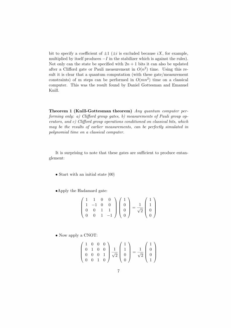
It is surprising to note that these gates are sufficient to produce entan-glement:

• Start with an initial state |00〉

•Apply the Hadamard gate:

1 1 0 01 −1 0 00 0 1 10 0 1 −1

1000

=

1√2

1100

• Now apply a CNOT:

1 0 0 00 1 0 00 0 0 10 0 1 0

1√2

1100

=

1√2

1001

7

This is the maximally entangled Bell state:

|ψ〉 =|00〉+ |11〉√

2

Again, it can be described by the Stabilizer generated by < X ⊗X,Z ⊗ Z >.

It is now clear that the presence of entanglement doesn’t automaticallybestow extra computational power. Amazingly, the Clifford gates and Paulimeasurements are also sufficient to perform teleportation.

Two very important gates which lie outside the Clifford Group are theToffoli gate and π/8 rotation of the Bloch sphere. One of these is requiredfor universal computation. In fact, any other gate outside the Cliffordgroup would do but these two are in a particularly convenient and usefulform already.

3 Simulating Entanglement

If Alice and Bob share the entangled state 1√2(|00〉 + |11〉) then standard

QM tells us:

If Alice performs a projective measurement on her qubit (in the Zdirection) she will obtain the result |0〉 (spin-up) with probability 1

2 or |1〉(spin-down) also with probability 1

2 .

If Bob then performs a measurement in the same basis he will obtaineither spin-up or spin down with 100% probability depending on Alice’sresult i.e. there is a total correlation between their results.

8

Using the normal convention for X,Y and Z measurement axes (see pic-ture of Bloch sphere above) we can list the transformations from one basisto another (ignoring normalization factors):

|+〉 ≈ |0〉+ |1〉|−〉 ≈ |0〉 − |1〉|0〉 ≈ |+〉+ |−〉|1〉 ≈ |+〉 − |−〉|p〉 ≈ |0〉+ i|1〉|m〉 ≈ |0〉 − i|1〉|0〉 ≈ |p〉+ |m〉|1〉 ≈ −i(|p〉 − |m〉)|p〉 ≈ α∗|+〉+ α|−〉|m〉 ≈ α|+〉 − α∗|−〉|+〉 ≈ α|p〉+ α∗|m〉|−〉 ≈ α∗|p〉+ α|m〉

Note: {|0〉, |1〉},{|p〉, |m〉} and {|+〉, |−〉} are the basis vectors for Z,Yand X respectively. Also, α = 1− i and α∗ = 1 + i.

Because this Bell state can be rewritten in the X basis as

|ψ〉 =|+ +〉+ | − −〉√

2

an equivalent correlation occurs if Alice and then Bob both measure inthe X basis ... either they both measure the state |+〉 or they both measure|−〉.

If the state is written in the Y basis then it is clear that if Alice and Bobboth measure in the Y basis they will obtain opposite results i.e. results are

9

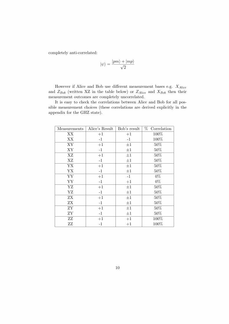
completely anti-correlated:

|ψ〉 =|pm〉+ |mp〉√

2

However if Alice and Bob use different measurement bases e.g. XAlice

and ZBob (written XZ in the table below) or ZAlice and XBob then theirmeasurement outcomes are completely uncorrelated.

It is easy to check the correlations between Alice and Bob for all pos-sible measurement choices (these correlations are derived explicitly in theappendix for the GHZ state).

Measurements Alice’s Result Bob’s result % CorrelationXX +1 +1 100%XX -1 -1 100%XY +1 ±1 50%XY -1 ±1 50%XZ +1 ±1 50%XZ -1 ±1 50%YX +1 ±1 50%YX -1 ±1 50%YY +1 -1 0%YY -1 +1 0%YZ +1 ±1 50%YZ -1 ±1 50%ZX +1 ±1 50%ZX -1 ±1 50%ZY +1 ±1 50%ZY -1 ±1 50%ZZ +1 +1 100%ZZ -1 +1 100%

10

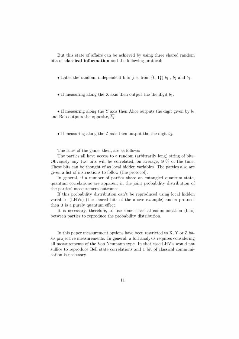
But this state of affairs can be achieved by using three shared randombits of classical information and the following protocol:

• Label the random, independent bits (i.e. from {0, 1}) b1 , b2 and b3.

• If measuring along the X axis then output the the digit b1.

• If measuring along the Y axis then Alice outputs the digit given by b2

and Bob outputs the opposite, b2.

• If measuring along the Z axis then output the the digit b3.

The rules of the game, then, are as follows:The parties all have access to a random (arbitrarily long) string of bits.

Obviously any two bits will be correlated, on average, 50% of the time.These bits can be thought of as local hidden variables. The parties also aregiven a list of instructions to follow (the protocol).

In general, if a number of parties share an entangled quantum state,quantum correlations are apparent in the joint probability distribution ofthe parties’ measurement outcomes.

If this probability distribution can’t be reproduced using local hiddenvariables (LHVs) (the shared bits of the above example) and a protocolthen it is a purely quantum effect.

It is necessary, therefore, to use some classical communication (bits)between parties to reproduce the probability distribution.

In this paper measurement options have been restricted to X, Y or Z ba-sis projective measurements. In general, a full analysis requires consideringall measurements of the Von Neumann type. In that case LHV’s would notsuffice to reproduce Bell state correlations and 1 bit of classical communi-cation is necessary.

11

In the literature there are two main models used to try to quantifythe amount of classical communication required, the bounded (worst-case)communication model and the average communication model. Here theworst-case model will be considered.

The previous example above did not require any classical communicationto simulate but others (e.g GHZ state) do.

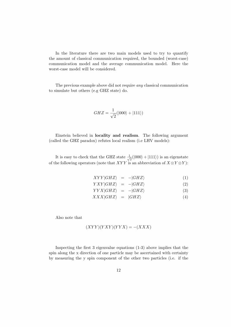
GHZ =1√2(|000〉+ |111〉)

Einstein believed in locality and realism. The following argument(called the GHZ paradox) refutes local realism (i.e LHV models):

It is easy to check that the GHZ state 1√2(|000〉+ |111〉) is an eigenstate

of the following operators (note that XY Y is an abbreviation of X⊗Y ⊗Y ):

XY Y |GHZ〉 = −|GHZ〉 (1)Y XY |GHZ〉 = −|GHZ〉 (2)Y Y X|GHZ〉 = −|GHZ〉 (3)XXX|GHZ〉 = |GHZ〉 (4)

Also note that

(XY Y )(Y XY )(Y Y X) = −(XXX)

Inspecting the first 3 eigenvalue equations (1-3) above implies that thespin along the x direction of one particle may be ascertained with certaintyby measuring the y spin component of the other two particles (i.e. if the

12

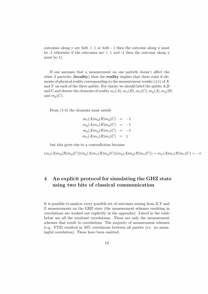
outcomes along y are both + 1 or both - 1 then the outcome along x mustbe -1 otherwise if the outcomes are + 1 and -1 then the outcome along xmust be 1).

If one assumes that a measurement on one particle doesn’t affect theother 2 particles (locality) then the reality implies that there exist 6 ele-ments of physical reality corresponding to the measurement results (±1) of Xand Y on each of the three qubits. For clarity we should label the qubits A,Band C and denote the elements of reality mx(A),mx(B),mx(C),my(A),my(B)and my(C).

From (1-4) the elements must satisfy

mx(A)my(B)my(C) = −1my(A)mx(B)my(C) = −1my(A)my(B)mx(C) = −1mx(A)mx(B)mx(C) = 1

but this gives rise to a contradiction because

(mx(A)my(B)my(C))(my(A)mx(B)my(C))(my(A)my(B)mx(C)) = mx(A)mx(B)mx(C) = −1

4 An explicit protocol for simulating the GHZ stateusing two bits of classical communication

It is possible to analyze every possible set of outcomes arising from X,Y andZ measurements on the GHZ state (the measurement schemes resulting incorrelations are worked out explicitly in the appendix). Listed in the tablebelow are all the resultant correlations. These are only the measurementschemes that result in correlations. The majority of measurement schemes(e.g. YYZ) resulted in 50% correlatons between all parties (i.e. no mean-ingful correlation). These have been omitted.

13

Measurement A’s outcome A-B A-C B-CScheme Correlation Correlation CorrelationXXX +1 50 50 100XXX −1 50 50 0XYY +1 50 50 0XYY −1 50 50 100XZZ +1 50 50 100XZZ −1 50 50 100YXY +1 50 50 100YXY −1 50 50 0YYX +1 50 50 0YYX −1 50 50 100YZZ +1 50 50 100YZZ −1 50 50 100ZXZ +1 50 100 50ZXZ −1 50 100 50ZYZ +1 50 100 50ZYZ −1 50 100 50ZZX +1 100 50 50ZZX −1 100 50 50ZZY +1 100 50 50ZZY −1 100 50 50ZZZ +1 100 100 100ZZZ −1 100 100 100

One protocol to simulate these correlations is as follows:

• If any of the parties measures along the Z axis, they output b1.

• Alice sends Bob a bit which tells him whether she performed an Xmeasurement or a Y measurement. If no bit is received then this indicatesthat Alice has performed a Z measurement. Regardless of whether she choseto do an X or Y measurement she outputs b2.

• Bob performs his measurement and tells Charlie what to output. If Bob

14

measures in the X basis then he outputs b3; if he measures in the Y basis heoutputs b3 In the cases where Bob has chosen to do the same measurementas Alice he sends the bit 0 to Charlie which tells him:“If you measure X output (b3 + b2)mod2. If you measure Y output b4”.In the cases where Bob decides to perform an X when A has measured Y orhe performs a Y when A has measured X then he sends the bit 1 to Charliewhich tells him:“ If you measure X output b4. If you measure Y output (b3+b2)mod2.” If nobit is sent (this happens when either Alice or Bob has decided to do a Z basismeasurement) then Charlie outputs b4 for either an X or Y measurement.

Two classical bits have been communicated in order to recreatethe correlations of the GHZ state.

This protocol is somewhat convoluted and doubtless can be improvedupon. The fact that Z measurements lead to not communicating a bitsuggests that the average communication cost is lower than two bits.

Any state that can be arrived at by using gates from the Clifford Groupand the initial state |0〉⊗n is called a stabilizer state. The GHZ state andmany other highly entangled states are stabilizer states. The stabilizer for-malism allows for measurements in the X,Y or Z direction only. It is aninteresting question, then, to consider the simulation of entangled states inthe context of the stabilizer formalism. In that context it might be possibleto formulate a generic protocol for the simulation of any stabilizer state.

5 Conclusion

Methods of quantifying the differences between quantum and classical in-formation have been discussed. It has been shown what quantum processesand measurements can be efficiently simulated on a classical computer. Twoprotocols for simulating entangled states using local hidden variables havebeen derived; one of which requires classical communication between parties.

15

6 Acknowledgements

The author would like to thank Dave Bacon for all his help and also all theCBSSS organizers especially Prof.s Erik Winfree and Andre Dehon.

References

Quantum Computation and Quantum Information by Michael A.Nielsen, Isaac L. Chuang. (2000)

Improved Simulation of Stabilizer Circuits Aaronson, Scott; Gottes-man, Daniel (2004-06-25) oai:arXiv.org:quant-ph/0406196

The Heisenberg Representation of Quantum Computers Gottes-man, Daniel (1998-07-01) oai:arXiv.org:quant-ph/9807006

The Communication Cost of Simulating Bell Correlations Toner,B F ; Bacon, D (2003-04-10) oai:arXiv.org:quant-ph/0304076

Theoretical investigations of separability and entanglement of bipartitequantum systems, Pranaw Rungta, Ph.D. in Physics, University ofNew Mexico, 2002

7 Appendix: Explicit Calculation of GHZ corre-lations

Note: |Ψ〉3 is a 3 qubit state; |γ〉2 is a 2-qubit state etc. If Alice performsa measurement and obtains the outcome +1 (−1) then this is denoted ⊕A

(ªA). Likewise when Bob performs a measurement we denote the outcome⊕B or ªB (N.B. These symbols are purely to denote measurement outcomesand have no relation to the operation of tensor addition).

Take |Ψ〉3 = |+ ++〉+ |+−−〉+ | −+−〉+ | − −+〉. If Alice measuresin the X basis then this collapses the state to one of two possible states,depending on her outcome: If she gets +1 then the state collapses to |α〉2 =

16

| + +〉 + | − −〉; if she gets -1 then it collapses to |β〉2 = | + −〉 + | − +〉.These new states will, in turn, be measured by Bob, again with possibleoutcomes ±1 and again collapsing the wavefunction to one of four possible1-qubit states: γ, δ, ε and φ.

To keep track of all possible sets of outcomes (and hence any possiblecorrelations), the measurement schemes will be written out as follows:

Measurement Scheme: XXXInitial State In X Basis: |Ψ〉3 = |+ ++〉+ |+−−〉+ | −+−〉+ | − −+〉

Alice Measures: ⊕A|α〉2 ªA|β〉2New State In X Basis |+ +〉+ | − −〉 |+−〉+ | −+〉

Bob Measures: ⊕A ⊕B |γ〉 ⊕A ªB |δ〉 ªA ⊕B |ε〉 ªA ªB |φ〉New State In X Basis |+〉 |−〉 |−〉 |+〉

A-B Correlations A-C Correlations B-C Correlations50% 50% 100%(⊕A), 0%(ªA)

Using a grid like that above it is obvious from the state’s position inthe grid what the previous measurement results were (e.g a state arrived atby Alice obtaining a +1 measurement and collapsing the wavefunction willalways be on the left hand side of the central dividing line). It can thereforebe written simply as:

Measurement Scheme: XXXInitial State In X Basis: |+ ++〉+ |+−−〉+ | −+−〉+ | − −+〉

Alice Measures: |+ +〉+ | − −〉 |+−〉+ | −+〉New State In X Basis |+ +〉+ | − −〉 |+−〉+ | −+〉

Bob Measures: |+〉 |−〉 |−〉 |+〉New State In X Basis |+〉 |−〉 |−〉 |+〉

A-B Correlations A-C Correlations B-C Correlations50% 50% 100%(⊕A), 0%(ªA)

17

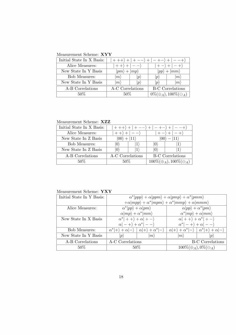
Measurement Scheme: XYYInitial State In X Basis: |+ ++〉+ |+−−〉+ | −+−〉+ | − −+〉

Alice Measures: |+ +〉+ | − −〉 |+−〉+ | −+〉New State In Y Basis |pm〉+ |mp〉 |pp〉+ |mm〉

Bob Measures: |m〉 |p〉 |p〉 |m〉New State In Y Basis |m〉 |p〉 |p〉 |m〉

A-B Correlations A-C Correlations B-C Correlations50% 50% 0%(⊕A), 100%(ªA)

Measurement Scheme: XZZInitial State In X Basis: |+ ++〉+ |+−−〉+ | −+−〉+ | − −+〉

Alice Measures: |+ +〉+ | − −〉 |+−〉+ | −+〉New State In Z Basis |00〉+ |11〉 |00〉 − |11〉

Bob Measures: |0〉 |1〉 |0〉 |1〉New State In Z Basis |0〉 |1〉 |0〉 |1〉

A-B Correlations A-C Correlations B-C Correlations50% 50% 100%(⊕A), 100%(ªA)

Measurement Scheme: YXYInitial State In Y Basis: α∗|ppp〉+ α|ppm〉+ α|pmp〉+ α∗|pmm〉

+α|mpp〉+ α∗|mpm〉+ α∗|mmp〉+ α|mmm〉Alice Measures: α∗|pp〉+ α|pm〉 α|pp〉+ α∗|pm〉

α|mp〉+ α∗|mm〉 α∗|mp〉+ α|mm〉New State In X Basis α∗|+ +〉+ α|+−〉 α|+ +〉+ α∗|+−〉

α| −+〉+ α∗| − −〉 α∗| −+〉+ α| − −〉Bob Measures: α∗|+〉+ α|−〉 α|+〉+ α∗|−〉 α|+〉+ α∗|−〉 α∗|+〉+ α|−〉

New State In Y Basis |p〉 |m〉 |m〉 |p〉A-B Correlations A-C Correlations B-C Correlations

50% 50% 100%(⊕A), 0%(ªA)

18

Measurement Scheme: YYXInitial State In Y Basis: α∗|ppp〉+ α|ppm〉+ α|pmp〉+ α∗|pmm〉

+α|mpp〉+ α∗|mpm〉+ α∗|mmp〉+ α|mmm〉Alice Measures: α∗|pp〉+ α|pm〉 α|pp〉+ α∗|pm〉

α|mp〉+ α∗|mm〉 α∗|mp〉+ α|mm〉New State In Y Basis α∗|pp〉+ α|pm〉 α|pp〉+ α∗|pm〉

α|mp〉+ α∗|mm〉 α∗|mp〉+ α|mm〉Bob Measures: α∗|p〉+ α|m〉 α|p〉+ α∗|m〉 α|+〉+ α∗|m〉 α∗|p〉+ α|m〉

New State In X Basis |−〉 |+〉 |+〉 |−〉A-B Correlations A-C Correlations B-C Correlations

50% 50% 0%(⊕A), 100%(ªA)

Measurement Scheme: YZZInitial State In Y Basis: α∗|ppp〉+ α|ppm〉+ α|pmp〉+ α∗|pmm〉

+α|mpp〉+ α∗|mpm〉+ α∗|mmp〉+ α|mmm〉Alice Measures: α∗|pp〉+ α|pm〉 α|pp〉+ α∗|pm〉

α|mp〉+ α∗|mm〉 α∗|mp〉+ α|mm〉New State In Z Basis |00〉+ i|11〉 |00〉 − i|11〉

Bob Measures: α∗|p〉+ α|m〉 α|p〉+ α∗|m〉 α|+〉α∗|m〉 α∗|p〉+ α|m〉New State In Z Basis |−〉 |+〉 |+〉 |−〉

A-B Correlations A-C Correlations B-C Correlations50% 50% 0%(⊕A), 100%(ªA)

19

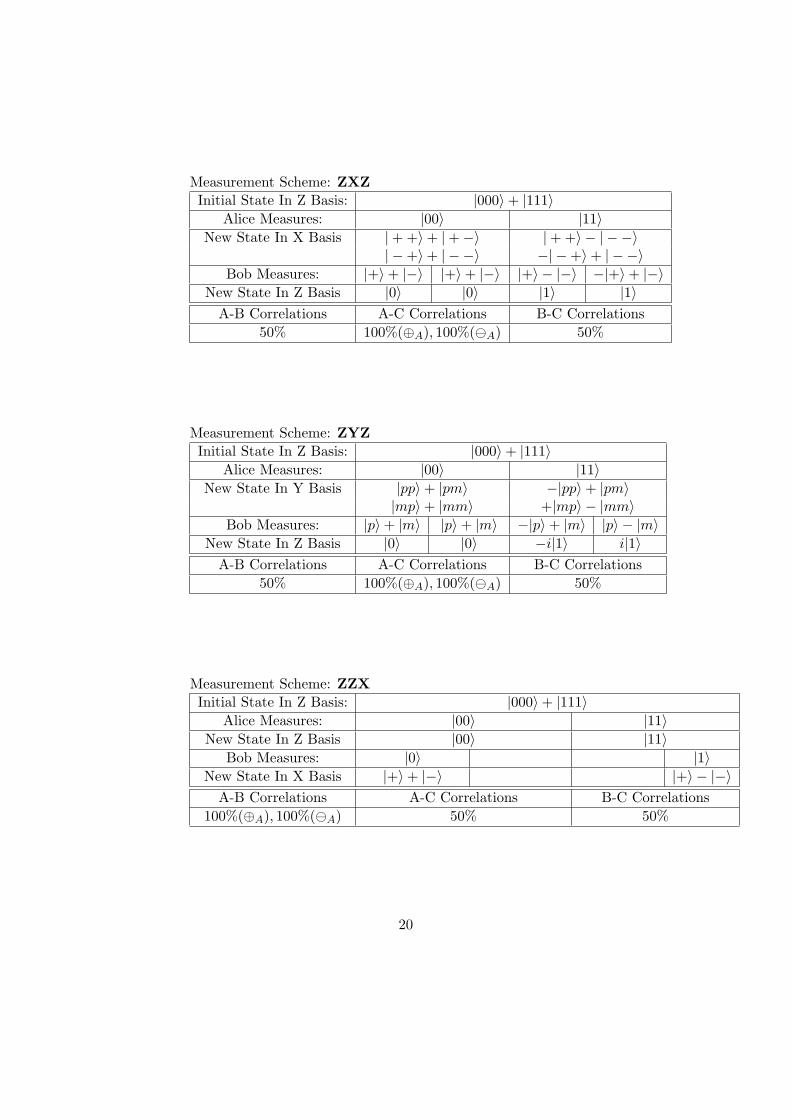
Measurement Scheme: ZXZInitial State In Z Basis: |000〉+ |111〉

Alice Measures: |00〉 |11〉New State In X Basis |+ +〉+ |+−〉 |+ +〉 − | − −〉

| −+〉+ | − −〉 −| −+〉+ | − −〉Bob Measures: |+〉+ |−〉 |+〉+ |−〉 |+〉 − |−〉 −|+〉+ |−〉

New State In Z Basis |0〉 |0〉 |1〉 |1〉A-B Correlations A-C Correlations B-C Correlations

50% 100%(⊕A), 100%(ªA) 50%

Measurement Scheme: ZYZInitial State In Z Basis: |000〉+ |111〉

Alice Measures: |00〉 |11〉New State In Y Basis |pp〉+ |pm〉 −|pp〉+ |pm〉

|mp〉+ |mm〉 +|mp〉 − |mm〉Bob Measures: |p〉+ |m〉 |p〉+ |m〉 −|p〉+ |m〉 |p〉 − |m〉

New State In Z Basis |0〉 |0〉 −i|1〉 i|1〉A-B Correlations A-C Correlations B-C Correlations

50% 100%(⊕A), 100%(ªA) 50%

Measurement Scheme: ZZXInitial State In Z Basis: |000〉+ |111〉

Alice Measures: |00〉 |11〉New State In Z Basis |00〉 |11〉

Bob Measures: |0〉 |1〉New State In X Basis |+〉+ |−〉 |+〉 − |−〉

A-B Correlations A-C Correlations B-C Correlations100%(⊕A), 100%(ªA) 50% 50%

20

Measurement Scheme: ZZYInitial State In Z Basis: |000〉+ |111〉

Alice Measures: |00〉 |11〉New State In Z Basis |00〉 |11〉

Bob Measures: |0〉 |1〉New State In Y Basis |p〉+ |m〉 −i(|p〉 − |m〉)

A-B Correlations A-C Correlations B-C Correlations100%(⊕A), 100%(ªA) 50% 50%

Measurement Scheme: ZZZInitial State In Z Basis: |000〉+ |111〉

Alice Measures: |00〉 |11〉New State In Z Basis |00〉 |11〉

Bob Measures: |0〉 |1〉New State In Z Basis |0〉 |1〉

A-B Correlations A-C Correlations B-C Correlations100%(⊕A), 100%(ªA) 100%(⊕A), 100%(ªA) 100%(⊕A), 100%(ªA)

21