This PDF is a selection from an out-of-print volume from the National Bureau of Economic Research

Volume Title: Annals of Economic and Social Measurement, Volume 1, number 4

Volume Author/Editor: NBER

Volume Publisher: NBER

Volume URL: http://www.nber.org/books/aesm72-4

Publication Date: October 1972

Chapter Title: Stabilization Policy and Lags: Summary and Extension

Chapter Author: J. Phillip Cooper, Stanley Fischer

Chapter URL: http://www.nber.org/chapters/c9444

Chapter pages in book: (p. 407 - 417)

Ann!s of Economic am! Social Aleasurenient, 1/4. 1972

STABILIZATION POLICY AND LAGS:SUMMARY AND EXTENSION*

BY J. PHILLIP COOPER ANt) STANLEY FISCHER

This paper examines the effect of both the length and tunability of higs on the effectiveness of counter-cyclical stabilization policy. The authors conclude that while th latter are an argument infwor of lessvigorous use of stabilization policy, the former are not. The lunger are lags, the more tigorousic shouldstabilization policy be used. They also find that in their models, the constant grouth raze ,'a!uc is neveroptimal and that the careful use offeedback controls is bound to be stabilizing.

INTRODUCTION

The major aim ofthis paper is to study the effects of both the length and variabilityof lags on the effectiveness of couritercyclical stabilization policy. The chief toolof analysis is a simple difference equation, in which the value of a target variable (y)is determined as a function of its lagged value and concurrent and lagged valuesof a policy variable(x) as well as an additive stochastic term (u) ; the policy variable(x,) is taken to be determined by a closed-loop feedback control rule responding tothe lagged value of the target variable (y 1)proportional control----and thechange in the value of the target variable (y,, - y,_2)derivative control.

The effectiveness of stabilization policy is evaluated by the value of theasymptotic variance of the target variable under the rules; various parametersof the difference equation determine both the mean length and the variability ofthe lags in the effect of policy. We are thus able to examine the results of changesin the length and variability of lags on the effectiveness of policy as policy isadjusted optimally (with respect to minimization of asymptotic variance) inresponse to these parameter changes. Our interest is not, however, confined tooptimal policies and we also investigate other properties of the system, such asits stability and sensitivity to nonoptimal choice of control rules, as lags vary.

In Section 1 below we very briefly summarize results obtained in our "CC"(constant coefficients) model in which all lag parameters are constant. The notionof variable lags and our representation of the notion through the randomizing oflag coefficients are discussed in Section 2, when our "RC model" is introduced.'The effects of the variability of lags as measured by the variance of the lagcoefficientson the outcome of policy rules is examined in Section 3. There isdiscussion in Sections 2 and 3 of the merits of a completely inactive policy whichavoids any attempts at "fine tuning"such policies have been recommended tothe monetary authorities by Friedman [2] and others.

sThe research described in this paper was supported by NSF Grant GS 29711. This is a much-shortened and somewhat changed version of our paper, "Stabilization Policy and Lags" which waspresented at the NSF-NBER Conference on Control Theory and Economic Systems. "StabilizationPolicy and Lags" is forthcoming in the Journal of Political Economy.

'Although the CC model is a special case of the RC model, it is convenient to treat them separatelyso that the effects of the length of lags can be discussed apart from the effects of their variability. Inaddition, there are certain results which we obtain analytically for the CC model but numerically forthe RC model.

407

This paper is a much-abbreviated summary of the paper presented at theNSF-NBER Conference on Control Theory afld Fconomic Systems which isforthcoming in the ,Iourna! of Political Lcono,n . Aside from the fact that manyresults are summarized hut not fully developed here, the other major changebetween the Conference paper and this one is that we here use a different stochasticprocess for the behavior ofthe random lag coefficients. The process, described hereas the "random [3" case, is one which we now regard as a fairer representation ofthe notion of variable lags in the context of discussion of the relative merits ofactive and inactive countercyclical policies than the "random 1." case preseitedin the Conference paper. Our reasons for this view are discussed later.

I. THE CC MODEL

A. 't'iodel Description

The model with constant coefficients is a standard first-order autoregressivescheme.

Yr = I3Yr - 1 + 1X. - + U,.iO

The restriction to a first-order autoregressive process is made for simplicity.The variable v, represents deviations of some economic variable from its

target level in each period and will be referred to as "output"; x, is to be under-stood as the deviations of some relevant instrument or policy variable (say, therate of change of the money supply) from that path which would, in the absenceof disturbances, keep the system on target at all times. Equation (I) may representthe reduced form of some structural model in which there is only one controllableexogenous variable. The value of u, is not known at the time the current value ofthe policy variable, X,, is chosen; information available at the time x, is chosenconsists of past levels of output and of the policy variable itself. The randomvariable u, has mean zero, is serially uncorrelated, and without loss of generalityhas variance unity. It is assumed that I/I < 1 so that the system is stable in theabsence ofan active stabilization policy (i.e. ifx, 0 for all t): generally we assumej3 positive.

The time form of the lag coeflicierits for the effects of policy, that is the z,of (1), is assumed proportional to a density function belonging to the Pascalfamily [5].

= (1 - A)').'r f i - 1 = 1,2,3,4,...

0<2<1.The parameters rand A determine thestructure ofthe coefTicients we concentrateon the cases r 1 and r = 2, particularly in the RC model below, but resultsholding for all members of the Pascal family are given in this section.

To standardize the long-run multiplier for monetary policy at unity, we setin (2) equal to (1 -. /3). It may be confirmed that then the ultimate efTect on thelevel of y obtained by increasing x by one unit and holding x at its higher levelforever, is to increase y by one unit, independent of the values of). and /3. We are

408

teIn

yC

C

a!

teIts

hevettre

thus assured that the "bang per buck" of policy stays constant for any permanentlyheld values of 2 and (I.

Two comments: first, the ;whicli we call the "direei'' (or "policy") lagcoefficientsdo not give the total effects on y, of a unit input of x at time t - i,for changes in x at t -- i change output at time t through the autoregressiveparameter /3 as well as directly. The level of output as a function of past levels ofthe policy variable and the random variable is

yt = 01x,_1 + fluUt

=i=o

This is a convolution of the previous lag coefficients and we refer to the c2 as the"Jinalform" lag distribution. For /3 = ), the final form lag coefficients are simplyPascal of order one higher than the order of the distribution for the themselves.

Second, we use a particular structure for the c and a particular autoregressivestructure in order to study the effects of the length of lags on stabilization policy;the mean final form lag of the effect of x on y is /31(1 - /3) + (rA)/(1 - A). Thelength of lag is thus an increasing function of r, 2 and /3.

The mean final form lag is the sum of the lag due to the autoregressivestructure (the "system" lag) and that due to the policy lag. Thus, by distinguishing/3 from A, we can discuss separately the effects of lags which are inherent in theeconomy (/3) from those due to policy (A and r). A long system lag (large /3) auto-matically implies a long final form lag though policy may work slowly even if /3is small.

B. The Constant Growth Rate Rule (CGRR)

We describe the policy x, = Ofor all las CGRR, i.e. a policy where no attemptis made to respond to deviations of y from trend. The asymptotic variance ofoutput under a constant growth rate rule is

where

The minimal attainable variance of)', is unity, obtained under any policy whichsucceeds in making y, = u, for all t. Thus if 1 = 0, the optimal policy is CGRR.If /3 is not zero, there is room for improvement by use of some policy other thanCGRRthe potential improvement increasing with IJ. It is useful to interpret /3

as a measure of the instability of the system in the absence of stabilization policyin much of what follows, the instability increasing as the system lag increases.

We shall refer to any policy which produces y, = u, as perfect control. Allother policies are imperfect control.

C. Policy Rules

The policy rules used are of the form

(6) x, = r(B). By,

409

(5) = E[y] =1

/32

where B is the backshift operator, and 1(B) is a polynomial in B of order a. Forinstance, one such rule with n = I is

x,=y1y,_1 --'i'2),-2 =g1y1 +g2(y,_1 -

where g1 is a proportional control and g2 a desivative control.Substituting (6), (5) and (2) in (1), and using the operator B, one obtains for

the general Pascal distribution:(1 - AB)rri

(1 - AB)'(l fiB) - (I - A)'(I - /1)1(B)B

which is an autoregressive moving-average model of order (r + I, r) when r a.By setting a rend choosing the coefficients in 1(B) appropriately it is alwayspossible to obtain

Ye =

which minimizes asymptotic variance-and also, any criterion function includingonly variances of output in each period. Thus optimal policies in the CC modelare straightforward to obtain.2

To have a better idea of the properties of such policies, we turn for simplicityto the case r = 1, although similar results apply also for other values of r. Theoptimal policy or r = 1 is to use rule (7) with

g2= (1fi)(1A)'There are a number of interesting features of the rule (10).

In this model, with perfect control, the proportional control dependsonly on the autoregressive parameter, and, in a sense, offsets the autoregressivecomponent of the model, while the derivative control deals also with the directlagged effects of policy.

Perhaps most interesting, the strength of the controls is an increasingfunction of the average length of lag, but increases in the length of lag do notincrease the variance of output.3

The use of negative feedback controls cannot lead to the minimumvariance policy if fi .c 0, that is, if the model itself, in the absence of control,contains only negative feedback.

We are also interested in the behavior of the system when policy is nonoptimal.Accordingly, we solved analytically for the value of the asymptotic variance 01the system as a function of fi, A and the parameters in the control rule, for values

2 It is easy to show that for perfect control,

r(B)-- fi (lABy- 1fl(lrObviously the second half of this sentence must be true if perfect control can be attained. A

stronger result is obtained in Howrey [3].

410

g1(JA

of r = 1 and r 2. This expression is used in defining the stability conditionsin terms of fi, A and the control parameters--for the system; it is also used todefine a region containing pairs of values of g1 and g2 which improve uponCGRR. Forthecasesr = landr = 2the followingadditional results are obtained

The longer are both policy and system lags, the more likely is the systemto be stable for given values of the control parameters.

Weak negative feedback controls are bound to be stabilizing relative toCGRR (for /?> 0).

The longer are both system and policy lags, the more likely is anychoice of control parameters to be stabilizing relative to CGRR.

In cases where insufficient control parameters are used, long lags reducethe potential gains from an active stabilization policy relative to CGRR ; however,they increase the likelihood that any given policy will be stabilizing relative toCGRR.

2. VARIABLE LAGS AND THE RC MODEL

Equation (I), the basic difference equation, can be rewritten as

= fiy11 + w, + u,where w represents the total direct effects of policy, past and present. For thePascal distribution with r = 1, the case on which we concentrate in this section,

w1 = (1 - fl)(1 - A)Ax,_1 = (1 - fl)(l - A)x1 + Aw_1.

In our random coefficients model, we continue to use (11) and (12) but modifythem by making fi a random variable. This has the effect of making both theautoregressive component and the effects of policy random. Specifically, we writefi instead of fi in both (11) and (12), and assume

1 + e,

where e has mean zero, variance a2, is serially uncorrelated and has zero covariancewith all u. Substituting fl1 for fin (11) and (12), the final form lag coefficients,

which give the total effects on the level of output in period of a unit changein x at time I - i, are

= (1 flt)(l - A) E A JJ fli-m+1j=O m1

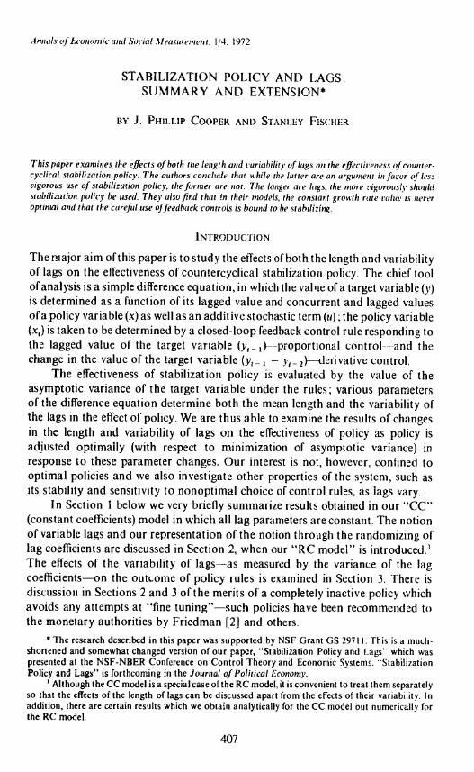
In Figure 1 we present final form lag distributions generated for the RCmodel with). = 0.8, fi (now the mean of the distribution off1) = 0.5, and r = I.The fi used in Figure 1 were drawn from a beta distribution-.---for which thedomain is [0, 1] with the variance a2 stated on the diagram. The three casesshown were chosen from a set of ten distributions generated and represent therange of examples produced.

The formulation described above is for obvious reasons called the "random /3"case. In the Conference paper we used the "random A" case in which A in (12)

411

Figure 1 Three Realizations of Final Form La Distributions r = J,. = 08, fi = 0.5, a2 = 0.0218)

is a random variable. In the random A case, randomness of the lag coefficientsaffects in the current period only the results of active countercyclical policy andnot CGRR; in the random fi case the results of both types of policy are affected.It can be shown that under CGRR

(15) I

Ifl2_2412

a

We believe it fairer to active policy to use the random fi model since we do notbelieve that CGRR would lead to any less variability of behavioral parametersthan other rules.

We believe that the lag formulations of (14), as shown in Figure 1, retlectthe notion of "variable lags." The time pattern of the effects of any particularpolicy action is not likely to be the same as those of any other policy action;the consequences of any particular policy action are known with certainty neitherin the period in which they are taken, nor in subsequent periods.

Our representation of variable lags treats these lags as stochastic, butvariability of lags is possible in a deterministic model. For instance, the lags ofmonetary policy could vary systematically with the behavior of other exogenousvariables in the economy, as they do in the FR B-MIT-Penn Econometric model.One might want to model variable lags by, say, having be a function of a variable,the time path of which is specified in some suitable way. This is another possibleroute, but it is not one we have so far taken.

For the case r = 2, which we have also examined we have instead of(12)(16) (1 - fl)(l -- ).)2x1 + 2Aw,_1 - A2w,_2

and then both the fi in (11) and that in (16) become fl1 with P determined asin (13).

Finally, we note an important point : our basic assumption for the RC modelis that the lags are "truly" stochasticthe distribution of the J3 is specified forall time.

3. RULES AND THE VARIANCE OF OUTPUT IN THE RC MODEL

Forthecaser = l,using(11)and(12)andthepoljcyrule(7),wjth$, = /? + ,we obtain

y1 [fi, +A+(1 flj(I 2)yjy,_1 + [Afl,_1 fiJ(1 - )Y21Y,-2= u, -

or

y, - by,.. + cy,_2 - (I - (1 - A)y1Jc,y,_ ± ),_ I)',- 2 + (I --= u, -

where

b=fl±A+(l --fl)(1 A)y

The question of the stability conditions for equation (18) now arises. Thereare a number of concepts of stochastic stability,4 and we shall use the finitenessof the asymptotic variance of output as our criterion; for if2 = 0 this gives thesame stability conditions as those for the CC model. This is a convenient definitionin view of the fact that we evaluate policies by this same criterion.

See Kozin [4] for discussion of some of these concepts.

413

(19) IT

(20)

(21)

Deriving the asymptotic variance of y1 from (18), we obtain

(I -I- c)(I 4-A2) - 22h - a2[o,2(I - A(h - 'i)) -(1 -- c) 1(1 + c12 - h2] o2{( I + e)a1 - ha 12 - b( - ')°21 -

+ (1 -- c2)a22 - a2[a 1(122 - a21a12]]where

a11 = (1 (1 - A)','1)(1 - (I - A)y - 2h) + (1 ))2y2 + A2

a12(1A.)y2[2(l --(I .))'1)i.b], a21A[1(1--A.))'1],22 = A(1 -

It is possible--though very tediousto show that

>0

>0(72

IgiOg2 = 0

aa2

for fi> 0

where g and g are the optimal proportional and derivative controls. Thus,the presence of slight variability of the lag coefficients leads to weaker derivativeand relatively stronger proportional controls than would be optimal in theabsence of the variability. (The proportional control may actually increaseabsolutely.) Basically, feedback controls use the level of output and changes inoutput as guides to the behavior of the additive error terim When lag coefficientsbecome variable, the level of output becomes a less safe guide to the behavior ofthe additive errorbut the change in output is doubly less safe.5 Thus, relativelymore weight is thrown on the proportional control.

It is clear that, in the RC model, we do not obtain certainty equivalenceresults. This is a consequence of the fact that the current policy variable, x,,affects current income subject to a multiplicative error.6

It can also be shownonce more at some lengththat

where means "of the same sign as."

g2 g,01g20

That is, the use of weak proportional or derivative controls is bound to hestabilizing relative to CGRR if /3 is positivewhatever the variability and lengthof the lags.

This explanation requires the first aulocovariance of income to be small, which it is at g2 = 0and with optimal control. (In fact, there is zero autocovaijance at this point.)6 See Brainard [1] for a fuller discussion of circumstances under which certainty equivalence isobtained. Our rules which give perfect control in the CC model arc certainly equivalence rules. Also,if in (II), we had made the first fi (that multiplying y, ) stochastic, and had otherwise had constantcoefficients, we would have obtained the same rules for the RC model as for the CCwhich illustratesthe certainty equivalence principle.

414

-2

-3

-5

7-24

3.73 3.0

2

-7

-s

-9

It is, unfortunately, difficult to minimize (19) analytically with respect toand y, to study the behavior of the system. Accordingly, we have used (19)

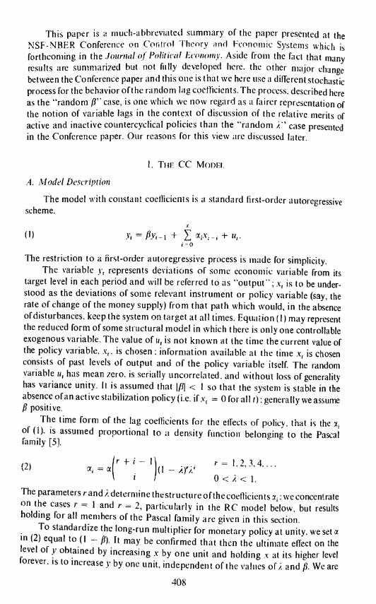
to compute optimal rules, stability regions and isovariance loci numerically fora number of combinations of A, fi and 72. In Figure 2 we present a typical diagram-for the case A = 0.8, Ii = 0.5, o = 0.0278---produced in our numerical analysis:the large shaded area is the stability region in that values of g1 and g, outsidethat area make the system completely unstable; the inner drawn locus is theCGRR isovariance locus-values of g1 and g2 within this region reduce variance

-20.6 -18.0 -15.4 - 12.8 - 10.2 -7.6 -5.0 -2.4 -0.2-IS ..........0 -7.:2

'.7-3.7.

7.7-

0.4

£770 VIII I, 0,7 . .13.65

Figure 2 Stability Area and Isovariance Contours for/I = 0.5,2 = 0.8, r = I. and a2 = 0.0278

415

,g2

- 111777 777)7.)3/ 3 777:'7;j757r '))s,7S-.'-*55S55).S''" 7)-

7fl1,,,,,:,,;,,,r,'.,'.','.'',,' n,)')S) . - ¶ 7l177 7777)7)53#))'3,?)P':'I 1 S. ,'n))'.3 3) 777P 7,77),),))Ut?,73),',))l't,,335,,)3 llll)!)73. 13))') 3 777 7,,r,,7nrn':: '':,sSS,,Sl) 13)) ),7'1)3:'%,).:,''3.;! SI

7-77777 17 SI3S,S 3)1), :''I')'''j''7),I.'',)flu 77l,73')))''u)')')'SS,S3,777771777f3:' 77)I7I)) 33)131.33 7),)') ))°,,')fl))) )3',),:3:', 2)

- 3)'77777777)71)) '7.';): 3,355') 7)I?3.).'I))')'''3''', 3)1) I:)S77711777 7))):7):r)-''')';..y.s ))

1777)7 '1,'))) ..........17777777137l7F:rI7'',-s.c ., 3:

7777n 11777'') 73,',' S )737':,n, .'',)'7)'''211

P ', , ,'''/ \

77l,Iln)17 1))flt''tS '7 3, ......7777777)1)?' ........77177 7777I77)''., 37731 3,33:':), -7777)3771I7?)) 5'..,

7777717717) In 53.) 3 7;.33' 33,777I17 717J37 ,,) 7757)3)) wIll

77tH 7??);),l,.;- 3,),:7777)7771)777 5))) 33)33:1777 7fl1777)' 35) )73))1,:34

55') 33)))',,'j'77)737777777 53'. )3)):3i.')7,7

777 :Ilrl,,,, y': ).-. .....

373)71777)1 31,').3I,);l7

- ' 7 77)77111I 55 3:))))) 311617717:7777 *33 3))) )3'fl7 736.77,71,lI'7 Sn)

-. ,,7;,;,:n ',:

- 1777 lflS3) 77)3:7-1),)'771771377'',' ._ 7:).

jfl 7-7S 63.) )jj 0. '7' 3I''.

3

'775

7717)ll1)) :3))' 5, ', 7

-4 --4.0

C.'

* Pr

ecis

ion

on th

ese

num

bers

diff

ers.

TAB

LE I

OP

TIM

AL

CO

NT

RO

LS A

ND

VA

RIA

NC

ES

FO

Rr =

1*

*

N .= N

a2 =

"N

.'

0.2

0.5

0.8

g1'

82*

a2g.

*a2

j*a

0,02

67-0

.200

-0.0

51.

042

1.07

1-0

.210

-0.1

81.

042

1.07

1-0

.231

-0.6

551.

045

1.07

10.

0145

-0.2

25-0

.05

1.02

31.

058

--0.

225

-0.2

11.

023

1.05

8-0

.243

-0.7

951.

025

1.05

80.

20.

0076

-0.2

35--

0.06

1.01

21.

050

-0.2

35-0

.23

1.01

21.

050

-0.2

48-0

.880

1.01

31.

050

0.00

35-0

.245

-0.0

61.

006

1.04

5-0

.245

-0.2

41.

006

1.04

5-0

.249

-0.9

501.

006

1.04

50.

0003

2--

0.25

0-0

.06

1.00

11.

042

-0.2

50-0

.25

1.00

11.

042

-0.2

50- 1

.000

1.00

11.

042

0-0

.25

-0.0

625

1.0

1.04

2-0

.25

-0.2

51.

01.

042

-0.2

5- 1

.01.

01.

042

0.02

78-0

.80

-0.2

01.

113

1.38

5-0

.86

-0.6

51.

123

1.38

5-1

.09

-2.1

51.

161

1.38

50.

0147

-0.9

0-0

.20

.060

1.36

0-0

.93

-0.8

01.

067

1.36

0-1

.15

-2.7

51.

093

1.36

00.

50.

0076

-0.9

3-0

.25

1.03

11.

347

-0.9

6-0

.90

1.03

51.

347

--1.

13-3

.25

1.05

21.

347

0.00

35-0

.97

-0.2

51.

014

1.34

0-0

.98

-0.9

51.

016

1.34

0-1

.09

-3.6

01.

025

1.34

00.

0003

1-1

.00

-0.2

51.

001

1.33

4-1

.00

-1.0

01.

001

1.33

4-1

.01

-3.9

51.

002

1.33

4

0-1

.0-0

.25

1.0

1.33

3-1

.0-1

.01.

01.

333

-1.0

-4.0

1.0

1.33

3

0.02

67-2

.05

-0.3

51.

680

3.00

0-2

.15

-1.1

01.

761

3.00

0-2

.55

-3.0

02.

022

3.00

00.

0145

-2.7

5-0

.50

1.37

32.

894

-2.9

0-1

.75

1.43

92.

894

-3.7

5-5

.25

1.65

82.

894

0.8

0.00

76-3

.30

-0.6

511

972.

838

-3.5

0-2

.40

1.24

32.

838

475

--7.

951.

400

2.83

80.

0035

-3.6

5-0

.80

1.09

12.

805

-3.8

5-3

.05

1.11

72.

805

-5.1

5-1

0.80

1.21

32.

805

0.00

032

-3.9

5-1

.00

1.00

82.

780

-4.0

0-3

.90

1.01

12.

780

-4.3

5-1

5.15

1.02

52.

780

0-4

.0-1

.01.

02.

778

-4.0

-4.0

1.0

2.77

8-4

.0-1

6.0

LU2.

778

below that obtained under CGRR; plus signs (+) and asterisks (*) trace the locion which the first-order conditions for g1 and g,, respectively, are satisiled; theoptimal values of g1 and g, are, of course, at the intersection of these two loci.

We produced such diagrams For values of A and /3 of 0.2. 0.5, and 0.8. andsix values of a2 for each of the nine combinations of). and /3. In each case we took/3, as belonging to the beta distribution, and computed the variance of /3, for anumber of integer-valued parameters of that distribution.7 It is perhaps worthemphasizing that the results presented below are not simulation results we usethe analytical expression (19) for the asymptotic variance of output to computeoptimal rules numerically.

Our major results are presented in Tables I and 2. Table 1 contains resultsfor r = 1, Table 2 results for r = 2. The four entries in a row for each combinationof A, /3 and a2 are, in order, the optimal g1 (g'), the optimal 2 (gfl, the value ofthe variance of output at the optimum (a), and the value of the variance underCGRR (o). In addition to the results of the tables, we shall mention resultsbased on examination of the diagrams such as Figure 2 for the cases presented.We consider now in turn the effects of changes in (A) the variability of lags, (B) thelength of the policy lag, (C) the length of the system lag.

TABLE 2

A. Variability of Lags

Most of these results are in accord with intuition.The minimal attainable variance increases with a2.For small a2, increases in a2 increase the relative strength of the propor-

tional control and decrease absolutely that of the derivative control; as a2continues to increase both controls are reduced absolutely. This result has beenexplained above. Note that the controls y and Y2 (equation (7)) both decrease instrength with a2.

The area of the outer stability region shrinks with a2-the larger is a2the more likely is any particular pair of controls to destabilize the system.

We used those integer parameters of the beta distribution which produced the maximumvariance for each value of the mean (/3 0.2 and 0.8), and then increased these parameters to reducethe variance of 8,. The maximum variance for/i = 0.5 is much larger than that for the other two cases:this larger variance, 0.0833, results from the degeneration of the beta distribution into the uniformdistribution. We do not present this case in Table I or Table 2.

417

OPTIMAL CONTROLS ANt) VARIANUS FOR I = 2. , 0.8, /3 = 0.5

3. = 0.8

0

/3 = 0.5 a2 = 0.0278 -0.5 -2.75 1.32 1.390.0147 -0.6 -4,5 1.26 1.360.0076 -0.7 -6.75 1.21 1.350.0035 -0.6 -9.0 1.17 1.340.00031 .Ø4 - 13.5 1.12 1.340 -0.36 -14.4 1.1 I 1.33