Stability of time–varying systems in the absence of strict

Lyapunov functions

Mohammad Fuad Mohammad Naser(1); Faycal Ikhouane(2)

(1)Faculty of Engineering Technology, Al-Balqa Applied University,Amman 11134, Jordan. E-mail: mohammad.naser@bau.edu.jo

(2) Universitat Politecnica de Catalunya, Department of Mathematics,Barcelona East School of Engineering, carrer Eduard Maristany,16, 08019, Barcelona, Spain. E-mail: faycal.ikhouane@upc.edu

Abstract

When a nonlinear system has a strict Lyapunov function, its stability can be studied usingstandard tools from Lyapunov stability theory. What happens when the strict conditionfails? This paper provides an answer to that question using a formulation that does notmake use of the specific structure of the system model. This formulation is then applied tothe study of the asymptotic stability of some classes of linear and nonlinear time-varyingsystems. Lyapunov functions, time-varying systems, (asymptotic) stability.

1. Introduction

This paper deals with the asymptotic stability of the nonlinear time–varying system x =f(t, x). When this system has a continuously differentiable Lyapunov function V that isstrict, standard results from Lyapunov stability theory establish the asymptotic stabilityof the origin [2, Theorem 3.2]. The strict condition on the Lyapunov function means thatthere exists a K –function β : R+ → R+ (that is β is continuous and strictly increasingwith β(0) = 0) that satisfies V (t, x) ≤ −β(|x|).

What happens when the strict condition does not hold? The following sufficient con-ditions imply asymptotic stability in the absence of the strict condition on V .

(i) The origin is asymptotically stable under the condition that there exists T > 0 suchthat for all t0, and x0: V

(t0 + T, x(t0 + T )

)− V (t0, x0) ≤ −β(|x0|) ([1]).

Preprint submitted to Elsevier January 22, 2020

(ii) A strict Lyapunov function can be constructed if we know a Lyapunov functionthat satisfies V (t, x) ≤ −W

(q(t), x

)for some periodic function q and a function W

positive definite in x (see [7]). The periodicity condition is weakened in [6].

(iii) The origin is asymptotically stable if V (t, x) ≤ −β(|x|) + γ(t − t0) for some L –function γ : R → R+; that is γ is continuous, nonnegative, nonincreasing andlimt→∞ γ (t) = 0 (see [8]).

(iv) Using the nested-Matrosov’s theorem, it can be shown that the origin is uniformlyglobally asymptotically stable if V (t, x) ≤ −β

(∣∣f(t, x)∣∣) where all time derivatives

of f are bounded [5, Corollary 2].

What happens when the Lyapunov function is not strict, and the aforementioned sufficientconditions do not hold? The initial motivation of the present paper was to propose ananswer to that question as follows: the origin is asymptotically stable if V (t, x) ≤ −h(t)|x|bfor some nonnegative function h such that

∫∞0h(t)dt = ∞. However, in the process

of proving this fact, we realized that this result can be obtained from a more generalformulation which be stated as follows: given a nonnegative absolutely continuous functionz whose explicit expression is not known, provide sufficient conditions on z so that (1) wehave an upper bound on z, and (2) we have limt→∞ z(t) = 0.

This formulation is given in Section 3 as Propositions 2 and 3. These two propositionsare applied to the asymptotic stability of nonlinear time–varying systems in Section 4.The main result of Section 4 is Theorem 6 which provides sufficient conditions for the(global) asymptotic stability of equilibria. Another application to Propositions 2 and 3 isprovided in Section 5 where we derive a new result on the asymptotic stability of perturbedlinear systems in Theorem 10. The main novelty of the result is that the perturbationsare allowed to be unbounded with respect to time. Conclusions are presented in Section6.

2. Terminology and notations

A real number x is said to be strictly positive when x > 0, strictly negative whenx < 0, nonpositive when x ≤ 0, and nonnegative when x ≥ 0. A function h : R → Ris said to be strictly increasing when t1 < t2 ⇒ h(t1) < h(t2), strictly decreasing whent1 < t2 ⇒ h(t1) > h(t2), nonincreasing when t1 < t2 ⇒ h(t1) ≥ h(t2), and nondecreasingwhen t1 < t2 ⇒ h(t1) ≤ h(t2).

1 The set of nonnegative integers is denoted N = 0, 1, . . .

1In this paper we avoid the use of the words “positive”, “negative”, “increasing”, “decreasing” as theymean different things in different books.

3

and the set of nonnegative real numbers is denoted R+ = [0,∞). The Lebesgue measure onR is denoted µ. We say that a subset of R is measurable when it is Lebesgue measurable.Let I ⊂ R+ be an interval, and consider a function p : I → Rl where l > 0 is an integer.We say that p is measurable when p is (Mµ, B)–measurable where B is the class of Borelsets of Rl and Mµ is the class of measurable sets of R+ (see [13]). For a measurablefunction p : I → Rl, ‖p‖I denotes the essential supremum of the function |p| on I where| · | is the Euclidean norm on Rl. When I = R+, this essential supremum is denoted‖p‖. C0(R,Rn) denotes the Banach space of continuous functions u : R → Rn endowedwith the uniform convergence norm ‖ · ‖. For each open interval I ⊂ R, the set of allcontinuously differentiable functions u : I → Rn is denoted C1(I,Rn).

3. Stability results

The main results of this section are Propositions 2 and 3 which provide an answerto the following question: consider an absolutely continuous function z ≥ 0; if we donot have the explicit expression of z, what kind of knowledge do we need in order to(1) establish an upper bound on z, and (2) show that limt→∞ z(t) = 0? The sufficientconditions provided in Propositions 2 and 3 generalise the following lemma from [9].

Lemma 1. [9, Lemma 17] Consider a function z : [t0, ω) → R+ where t0 ∈ R andt0 < ω ≤ ∞. Assume that Conditions (i)–(ii) hold.

(i) The function z is absolutely continuous on each compact interval of [t0, ω).

(ii) There exist z1 ≥ 0 and z2 > 0 such that z1 < z2, z (t0) < z2 and z (t) ≤ 0 for almostall t ∈ (t0, ω) that satisfy z1 < z (t) < z2.

Then z (t) ≤ max (z (t0) , z1), ∀t ∈ [t0, ω).

Proposition 2. Consider a function z : [t0, ω) → R+ where t0 ∈ R and t0 < ω ≤ ∞.Assume that Conditions (i)–(iii) hold.

(i) The function z is absolutely continuous on each compact interval of [t0, ω).(ii) There exist functions ϕ, ψ : [t0, ω)→ R+ such that

(ii)–1 both ϕ and ψ are absolutely continuous on each compact interval of [t0, ω),(ii)–2 and Inequalities (9)–(10) hold,

ϕ (t) < ψ (t) ,∀t ∈ [t0, ω), (1)

z (t) ≤ min(ϕ (t) , ψ (t)

), for almost all t ∈ (t0, ω)

that satisfy ϕ (t) < z (t) < ψ (t) .(2)

4

(iii) z (t0) ≤ ϕ (t0).

Thenz (t) ≤ ϕ (t) , ∀t ∈ [t0, ω). (3)

Furthermore, if ϕ is nonincreasing and

z (t) ≤ 0, for almost all t ∈ (t0, ω) that satisfy z (t) < ϕ (t) , (4)

thenz (t) ≤ min (z (t0) , ϕ (t)), ∀t ∈ [t0, ω). (5)

Proof. The aim of the following analysis is to prove that Inequality (3) holds. To this end,we use an argument by contradiction. Assume that there exists some t1 ∈ (t0, ω) such thatz (t1) > ϕ (t1). Consider the set C = τ ∈ [t0, ω)/ z (t) ≤ ϕ (t) , for all t ∈ [t0, τ ]. Theset C is nonempty because t0 ∈ C. Define t2 = sup C. Observe that t2 ≤ t1 <∞ becauseotherwise we have t1 ∈ C which contradicts the fact that z(t1) > ϕ(t1). By the definitionof t2, there exists a real sequence τn ∈ C∞n=1 such that limn→∞ τn = t2. The continuityof functions z and ϕ implies that z (t2) = limn→∞ z (τn) ≤ limn→∞ ϕ (τn) = ϕ (t2). Thisfact implies that t2 ∈ C leading to t2 < t1. Also, there exists a real sequence τ ′n > t2∞n=1

such that z (τ ′n) > ϕ (τ ′n) , for all n ∈ N and limn→∞ τ′n = t2. Since z and ϕ are continuous

we get z (t2) ≥ ϕ (t2) which leads to z (t2) = ϕ (t2).

Let D = t ∈ [t2, t1] / z (t) = ϕ (t). The set D is nonempty because t2 ∈ D. Definet3 = sup D, then using a similar argument as above we get t3 ∈ D which implies thatz(t3) = ϕ (t3) and t3 < t1.

Claim 1. For all t3 < t ≤ t1, z (t) > ϕ (t) .Proof. To prove the claim we use an argument by contradiction. Assume that thereexists t4 ∈ (t3, t1] such that z (t4) ≤ ϕ (t4). By the definition of t3, we get z (t4) < ϕ (t4).Define the function z1 : [t0, ω) → R as z1 (t) = z (t) − ϕ (t) , for all t ∈ [t0, ω). Thefunction z1 is continuous and satisfies z1 (t4) < 0 and z1 (t1) > 0. Thus we conclude fromthe Intermediate Value Theorem that there exists some t5 ∈ (t4, t1) such that z1 (t5) = 0so that z (t5) = ϕ (t5) which implies that t5 ∈ D. This is not possible since t5 > t3. Theproof of Claim 1 has been completed.

Let E = t ∈ (t3, t1]/ z (t) = ψ (t). Define

t6 =

t1 if E = ∅inf E if E 6= ∅

5

Claim 2. z (t6) > ϕ (t6).Proof. If E = ∅, then t6 = t1 and thus z (t6) > ϕ (t6). If E 6= ∅, then t6 = inf E andthus the continuity of z and ψ implies that t6 ∈ E, so that z (t6) = ψ (t6) and hence weget from (9) that z (t6) > ϕ (t6). Thus, in all cases we have z (t6) > ϕ (t6).

Claim 3. z (t) < ψ (t) , for all t3 < t < t6.Proof. If E = ∅, then t6 = t1. We need to show that z (t) < ψ (t) , for all t3 < t < t6.To this end, assume that there exists t′6 ∈ (t3, t6) such that z (t′6) ≥ ψ (t′6). Since E = ∅,we have z (t′6) > ψ (t′6). Thus we deduce by Inequality (9) and the fact z(t3) = ϕ (t3) that

z1 (t′6) > 0 = z (t3)− ϕ (t3) > z (t3)− ψ (t3) = z1 (t3) ,

where z1 (·) = z (·) − ψ (·). Therefore, by applying the Intermediate Value Theorem onthe continuous function z1 (·) and on the interval [t3, t

′6], we deduce that E 6= ∅ which is

a contradiction. This proves that z (t) < ψ (t) , for all t3 < t < t6.If E 6= ∅, it can be shown by the continuity of z and ψ that t6 = inf E ∈ E so thatz (t6) = ψ (t6). We need to show that z (t) < ψ (t) , for all t3 < t < t6. To this end,assume that there exists t′′6 ∈ (t3, t6) such that z (t′′6) ≥ ψ (t′′6). Since t6 = inf E, we havez (t′′6) > ψ (t′′6). Thus we deduce by Inequality (9) and the fact z(t3) = ϕ (t3) that

z1 (t′′6) > 0 = z (t3)− ϕ (t3) > z (t3)− ψ (t3) = z1 (t3) ,

where z1 (·) = z (·) − ψ (·). Therefore, by applying the Intermediate Value Theorem onthe continuous function z1 (·) and on the interval [t3, t

′′6], we deduce that there exists

t′′′6 ∈ (t3, t′′6) such that z1 (t′′′6 ) = 0 so that z (t′′′6 ) = ψ (t′′′6 ). This contradicts the facts that

t6 = inf E and t3 < t′′′6 < t′′6 < t6 and thus z (t) < ψ (t) , for all t3 < t < t6. This end theproof of Claim 3.

Since t3 < t6 ≤ t1, we get from Claims 1 and 3 that

ϕ (t) < z (t) < ψ (t) , ∀t3 < t < t6. (6)

Thus we obtain by (10) that z (t) ≤ ϕ (t) , for almost all t ∈ (t3, t6). Hence the absolutecontinuity of functions z and ϕ leads to z (t6) − z (t3) =

∫ t6t3z (τ) dτ ≤

∫ t6t3ϕ (τ) dτ =

ϕ (t6) − ϕ (t3) and thus we obtain by the fact z (t3) = ϕ (t3) that z (t6) ≤ ϕ (t6) whichcontradicts Claim 2.As a summary, we have proved that

z (t) ≤ ϕ (t) , ∀t ∈ [t0, ω), (7)

6

which proves (3).

We need to prove that Inequality (5) is true whenever (4) is satisfied and ϕ is nonin-creasing. To this end, we prove that z (t) ≤ z (t0) , for all t ∈ [t0, ω) for both situationsz (t0) = ϕ (t0) and z (t0) < ϕ (t0).

If z (t0) = ϕ (t0), then since ϕ is nonincreasing, we obtain from (7) that

z (t) ≤ ϕ (t) ≤ ϕ (t0) = z (t0) , for all t ∈ [t0, ω),

which means that (5) is satisfied.

If z (t0) < ϕ (t0), suppose that there exists t7 ∈ (t0, ω) such that z (t7) > z (t0). Thenϕ (t0) > 0 (because if ϕ (t0) = 0, then z (t0) < 0 which is a contradiction). Let S =t ∈ (t0, t7]/ z (t) = ϕ (t). We now show that S cannot be empty. To this end, assumethat S = ∅. Using (7) and the continuity of z and ϕ, a simple contradiction argumentproves that z (t) < ϕ (t) , for all t ∈ [t0, t7). Hence we obtain from (4) that z (t7)−z (t0) =∫ t7t0z (τ) dτ ≤ 0 so that z (t7) ≤ z (t0). This contradicts the assumption z (t7) > z (t0).

Thus S 6= ∅. Let t8 = inf S. Using (7) and the continuity of z and ϕ, a simple contradictionargument proves that t0 < t8 ≤ t7 and z (t) < ϕ (t) , for all t ∈ [t0, t8). Hence we obtainfrom (4) that z (t8)− z (t0) =

∫ t8t0z (τ) dτ ≤ 0 so that

z (t8) ≤ z (t0) . (8)

The continuity of the functions z and ϕ implies that t8 = inf S ∈ S so that z (t8) = ϕ (t8).Therefore, since ϕ is nonincreasing and t0 < t8 ≤ t7, we get from (7) that

z (t8) = ϕ (t8) ≥ ϕ (t7) ≥ z (t7) > z (t0) ,

which contradicts (8). Thus, Inequality (5) is satisfied and the proof has been completed.

Proposition 3. Consider a function z : [t0, ω) → R+ where t0 ∈ R and t0 < ω ≤ ∞.Assume that Conditions (i)–(iii) hold.

(i) The function z is absolutely continuous on each compact interval of [t0, ω).

(ii) There exist functions ϕ, ψ : [t0, ω)→ R+ such that

(ii)–1 both ϕ and ψ are absolutely continuous on each compact interval of [t0, ω),

7

(ii)–2 and Inequalities (9)–(10) hold,

ϕ (t) < ψ (t) ,∀t ∈ [t0, ω), (9)

z (t) ≤ min(ϕ (t) , ψ (t)

), for almost all t ∈ (t0, ω)

that satisfy ϕ (t) < z (t) < ψ (t) .(10)

(iii) z (t0) ∈ (ϕ (t0) , ψ (t0)).

Thenz (t) < ψ (t) ,∀t ∈ [t0, ω). (11)

Assume furthermore that ω =∞ and that there exist a measurable function q : [t0,∞)→R+ and a nondecreasing measurable function H : R+ → R+ such that Equations (12)–(14)hold.

H (0) = 0 and H (v) > 0, ∀v > 0, (12)

z (t) ≤ −q (t) H (z (t)) , for almost all t ∈ (t0,∞)

that satisfy ϕ (t) < z (t) < ψ (t) ,(13)

limt→∞

t∫t0

q (τ) dτ =∞. (14)

Then (a) and (b) hold.

(a) If L = limt→∞ ϕ (t) = 0, we have limt→∞ z (t) = 0.

(b) If L = limt→∞ ϕ (t) does not exist, is infinite, or exists with L > 0, then there existsT ∈ (t0, ω) such that

ϕ (t) < z (t) ≤ z (t0) ,∀t ∈ [t0, T ),

z (T ) = ϕ (T ) ,

z (t) ≤ ϕ (t) ,∀t ∈ (T,∞) .

(15)

8

Proof. The aim of the following analysis is to prove Inequality (11). To this end, considerthe set B = t ∈ (t0, ω) / z (t) = ϕ (t).

IfB = ∅, assume that there exists t1 ∈ (t0, ω) with z (t1) ≥ ψ (t1). Let J = t ∈ (t0, ω) / z (t) = ψ (t).Using Intermediate Value Theorem, it can be verified that J 6= ∅. Let t2 = inf J . Thenfor all t ∈ [t0, t2) we have z(t) < ψ (t). One can use the Intermediate Value Theorem

to prove that ϕ (t) < z(t), for all t ∈ [t0, t2). These facts along with (10) imply that foralmost all t ∈ (t0, t2) we have z(t) ≤ ψ (t). Since z and ψ are absolutely continuous, itfollows that z(t2) − z(t0) =

∫ t2t0z(τ) dτ ≤

∫ t2t0ψ(τ) dτ = ψ (t2) − ψ(t0). This contradicts

the facts that z (t2) = ψ (t2) and ψ (t0) > z (t0) and thus

z(t) < ψ(t),∀t ∈ [t0, ω) whenever B = ∅.

If B 6= ∅, then t3 = inf B ∈ B because of the continuity of z and ϕ. Thus seeing t3 as aninitial time, and ϕ (t3) as an initial condition, it follows from Proposition 2 that for allt ∈ [t3, ω) we have z(t) ≤ ϕ (t). Using the same analysis used for B = ∅, it can be shownthat z(t) < ψ(t) for all t ∈ [t0, t3). We summarize the previous results as

z(t) < ψ(t) ∀t ∈ [t0, t3)

z(t) ≤ ϕ (t) ∀t ∈ [t3, ω)whenever B 6= ∅

and thus Inequality (9) implies that z(t) < ψ(t) for all t ∈ [t0, ω), whenever B 6= ∅.

We conclude that, in both situations B = ∅ and B 6= ∅, Inequality (11) is satisfied.To complete the proof assume that ω =∞ and that there exist a measurable function

q : [t0,∞)→ R+ and a nondecreasing measurable function H : R+ → R+ for which (12),(13) and (14) are satisfied. Let A = t ∈ [t0,∞)/ z (t) = ϕ (t).

Claim 1. If A = ∅, then limt→∞ z (t) = limt→∞ ϕ (t) = 0.Proof. Since A = ∅, Inequality (11) and a simple contradiction argument prove that

ϕ (t) < z (t) < ψ (t) ,∀t ∈ [t0,∞). (16)

Thus, we obtain from (13) that z (t) ≤ 0 for almost all t ∈ (t0,∞) because the functionsq and H are nonnegative. Thus z is nonincreasing on [t0,∞) so that limt→∞ z (t) = L∗exists with z (t) ≥ L∗ ≥ 0 for all t ∈ [t0,∞).

If L∗ > 0 then, from (16), (13) and for all t ∈ [t0,∞), z (t) ≥ L∗, it follows that

z (t) ≤ −ε q (t) , for almost all t ∈ (t0,∞) ,

9

where ε = H (L∗) is strictly positive because of (12). Thus, the Fundamental Theorem ofCalculus implies that

z (t) = z (t0) +

t∫t0

z (τ) dτ ≤ z (t0)− εt∫

t0

q (t) , ∀t ∈ [t0,∞),

which leads to limt→∞ z (t) = −∞ because of (14). This contradiction proves thatL∗ = limt→∞ z (t) = 0 and thus we obtain from (16) that limt→∞ ϕ (t) = 0. This fin-ishes the proof of Claim 1.

Claim 2. If A 6= ∅, then there exists T ∈ (t0, ω) such that (15) is satisfied.Proof. The continuity of z and ϕ implies that T = inf A ∈ A so that z (T ) = ϕ (T ). Itcan be easily verified using (13) and (11) that ϕ (t) < z (t) ≤ z (t0) for all t ∈ [t0, T ). Now,seeing T as an initial time and ϕ (T ) as an initial condition, we obtain from Proposition2 that z (t) ≤ ϕ (t) for all t ∈ (T,∞). Therefore (15) is satisfied.

If limt→∞ ϕ (t) = 0, we deduce from Claims 1 and 2 that limt→∞ z (t) = 0. Otherwise,we get from Claim 1 that A 6= ∅ and thus (15) is satisfied because of Claim 2. Thiscompletes the proof.

The following corollary provides sufficient conditions to get limt→∞ z (t) = 0.

Corollary 4. Suppose that Conditions (a)–(e) hold.

(a) Conditions (i) and (ii) of Proposition 2 are satisfied,

(b) ω =∞,

(c) limt→∞ ϕ (t) = 0,

(d) z (t0) < ψ (t0),

(e) there exist a measurable function q : [t0,∞)→ R+ and a nondecreasing measurablefunction H : R+ → R+ for which Equations (12), (13) and (14) are satisfied.

Then limt→∞ z (t) = 0.

Proof. The result follows by considering the cases z (t0) ≤ ϕ (t0) and z (t0) ∈ (ϕ (t0) , ψ (t0))along with Proposition 2 and 3 respectively.

Remark. In [10] an attractiveness result is obtained using a different formulation andwith different assumptions. It roughly says that when the derivative of some function isless than the sum of a negative function of the state and a ‘small’ -in some sense- function

10

of the state, we get some kind of asymptotic convergence of the state to zero. This resultis not directly related to Propositions 2 and 3 because the right-hand side of Inequality(13) contains two separate parts: a term that depends on the state and another thatdepends on time.

4. Asymptotic stability of a class of nonlinear time–varying systems

The aim of this section is to study the asymptotic stability of system (17)–(18)

x(t) = f(t, x(t)

), t ∈ R+, (17)

x(t0) = x0, (18)

where (t0, x0) ∈ R+×Rm, state x(t) take values in Rm for some strictly positive integer m,and function f : [t0,∞)×Rm → Rm is well-defined. Section 4.1 presents a brief summaryof the results provided in [2] regarding the existence of solutions of the differential equation(17)–(18). In Section 4.2 we present the stability definitions that are used throughout thepaper. Section 4.3 gives sufficient conditions for the asymptotic stability of the system(17).

4.1. Caratheodory solutions

The following set of assumptions for (17)–(18) is considered in [2, Section 1.1].

(A1) The function f(t, x) is locally essentially bounded on R+ × Rm,(A2) for each x ∈ Rm, the function t 7→ f(t, x) is measurable,(A3) for almost all t ∈ R+, the function x 7→ f(t, x) is continuous.

A function x is called a local Caratheodory solution of (17)–(18) on the interval I ⊂ R+

if t0 ∈ I, the function x is absolutely continuous on every compact subinterval of I andsatisfies

x(t) = f(t, x(t)

), for almost all t ∈ I, (19)

x(t0) = x0. (20)

Caratheodory’s Theorem states that if Assumptions (A1)–(A3) hold then for each initialpair (t0, x0) ∈ R+×Rm, then there exists an interval I ⊂ R+ with t0 ∈ I such that a localCaratheodory solution (19)-(20) exists on I.

If the function f is continuous on R+×Rm then Assumptions (A1)–(A3) are satisfied.By Peano’s Theorem it follows that a classical solution x of (17)–(18) exists on someinterval t0 ∈ I ⊂ R+. The term “classical” means that x is of class C1 and

x(t) = f(t, x(t)

),∀t ∈ I, (21)

x(t0) = x0. (22)

11

4.2. Stability definitions

In this section and in the remaining sections we assume that Assumptions (A1)–(A3)hold so that at least one local Caratheodory solution (19)-(20) exists on some intervalt0 ∈ I ⊂ R+.

Definition 5. [2, p.79] The point x = 0 of the system (17) is said to be

(i) an equilibrium point if f (t, 0) = 0 for almost all t ≥ 0,

(ii) locally attractive if for each t0 ∈ R+, there exists c > 0 such that if |x0| < c, theneach solution x of (17)–(18) is continuable on [t0,∞) with limt→∞ x (t) = 0,

(iii) globally attractive if for all t0 ∈ R+ and all x0 ∈ Rm, each solution x of (17)–(18)is continuable on [t0,∞) with limt→∞ x (t) = 0,

(iv) stable if for any t0 ∈ R+ and any ε > 0, there is c > 0 such that if |x0| < c theneach solution x of (17)–(18) is continuable on [t0,∞) and

|x (t)| < ε, ∀t ≥ t0,

(v) uniformly stable if for any ε > 0, there is c > 0 such that for each t0 ∈ R+ and each|x0| < c, every solution x of (17)–(18) is continuable on [t0,∞) and

|x (t)| < ε, ∀t ≥ t0,

(vi) asymptotically stable if it is stable and locally attractive,

(vii) globally asymptotically stable if it is stable and globally attractive.

4.3. Sufficient conditions for the asymptotic stability

In this section we use Proposition 2 and 3 to study the asymptotic stability of thesystem (17)–(18). The main result is given in Theorem 6.

For any t0 ∈ R define the set

Ω2(t0) =

h : R→ R+/ h is Lebesgue measurable with

∞∫t0

h(s)ds =∞

.

Theorem 6. Consider the system (17)–(18) for which Assumptions (A1)–(A3) are satis-fied. Assume that Conditions (i)–(ii) hold.

12

(i) The origin x = 0 is an equilibrium point for the system (17).

(ii) There exists a function h ∈ Ω2(t0) such that for each solution x of (17)-(18) withmaximal interval of existence [t0, ω) there exist positive constants δ, a, b, k1, k2, anda function V ∈ C1 (R× Rm,R+), satisfying

k1 |α|a ≤ V (t, α) ≤ k2 |α|a ,∀t ∈ [t0, ω),∀α ∈ Rm, (23)

∂V (t, α)

∂t

∣∣∣∣α=x(t)

+∂V (t, α)

∂α

∣∣∣∣α=x(t)

· f (t, x (t)) ≤ −h (t) |x (t)|b , (24)

for almost all t ∈ (t0, ω) that satisfy |x (t)| < δ.

Then

(i) All solutions of (17)-(18) are defined on [t0,∞) for any initial condition |x0| <a

√k1k2δ;

(ii) moreover, the origin x = 0 is uniformly stable and asymptotically stable.

Additionally, if Inequality (24) is satisfied for δ =∞ then x = 0 is globally asymptoticallystable.

Before giving the proof of Theorem 6 we compare it to the results obtained in [6].That reference considers systems of the form x = f (x, u) in which u is the input, andx(t0) = x0 is the initial condition. Consider the set

Ω1(t0) =

h ∈ C0 (R,R+) / ∃τ, ε, h > 0 satisfying

t∫t−τ

h(s)ds ≥ ε and h (t) ≤ h,∀t ≥ t0

.

If there exists a C1 Lyapunov function V such that ddtV(t, x(t), u(t)

)≤ −h(t)β1 (|x(t)|)

for almost all t > t0 with |x(t)| ≥ β2 (|u(t)|) for some h ∈ Ω1, β1 ∈ K∞ ∩ C1 and someβ2 ∈ K∞, then the system is input-to-state stable (see Definition 1 and Theorem 5 in [6]).

Any continuous periodic function that is not identically zero belongs to the set Ω1. Ad-ditionally, there are nonperiodic functions that belong to Ω1 [6, p. 3].

The contribution of Theorem 6 is to provide sufficient conditions for the asymptoticstability of (17)–(18) for functions h that belong to the set Ω2 which is larger than Ω1.

13

Proposition 7. Ω1 ⊂ Ω2 and Ω2 \ Ω1 is nonempty.

Proof. To prove that Ω1 ⊂ Ω2, assume that there exists a function h : R→ R+ such thath ∈ Ω1 and h /∈ Ω2. Since h ∈ Ω1, then h is continuous (and hence Lebesgue measurable)and there exist τ > 0 and there exists ε > 0 such that

∫ tt−τ h(s)ds ≥ ε for all t ≥ t0. On

the other hand, since h /∈ Ω2, then∫∞t0h(s)ds 6= ∞. Thus

∫∞t0h(s)ds = w ∈ R+ since

h ≥ 0. On the other hand, we conclude by the inequality∫ tt−τ h(s)ds ≥ ε for all t ≥ t0

that∫ t0t−τ h(s)ds +

∫ tt0h(s)ds ≥ ε for all t ≥ t0. Taking t → ∞ leads to the contradiction

−w + w = 0 ≥ ε. Therefore Ω1 ⊂ Ω2.To prove that Ω2 \ Ω1 is nonempty, consider the continuous function h : R → R

defined by h(t) = 1t+1

for all t ≥ t0 and h(t) = 1t0+1

for all t ≤ t0. Then∫∞t0h(s)ds = ∞

so that h ∈ Ω2. Suppose that there exist τ > 0 and ε > 0 such that for all t ≥ t0 + τ ,∫ tt−τ h(s)ds = ln

(t+1

t−τ+1

)≥ ε. Taking t → ∞ leads to a contradiction which shows that

h ∈ Ω2 \ Ω1.Another example is h : R→ R defined by h(t) = t for all t ∈ R which is in Ω2 \Ω1.

We now present the proof of Theorem 6.

Proof of Theorem 6. Let x be a solution of (17)–(18) with maximal interval of existence[t0, ω). Define z : [t0, ω)→ R+ as z (t) = V (t, x (t)) for all t ∈ [t0, ω). Since x is absolutelycontinuous and V is continuously differentiable, the function z is absolutely continuouson each compact interval of [t0, ω). Therefore, Condition (i) of Lemma 1 is satisfied.We get from (24) and (23) that

z (t) =∂V (t, α)

∂t

∣∣∣∣α=x(t)

+∂V (t, α)

∂α

∣∣∣∣α=x(t)

· f (t, x (t)) ≤ 0.

for almost all t ∈ (t0, ω) that satisfy 0 < z (t) < k1δa. Thus Condition (ii) of Lemma 1 is

satisfied with z1 = 0 and z2 = k1δa. It follows from Lemma 1 that if z (t0) < z2 = k1δ

a

then z (t) ≤ z (t0) for all t ∈ [t0, ω). This fact combined with Inequalities (23) leads to

|x (t)| ≤ a

√k2k1|x0| ,∀t ∈ [t0, ω) whenever |x0| < a

√k1k2δ.

It also follows that ω =∞ whenever |x0| < a

√k1k2δ [11, p. 71]. These facts mean that the

equilibrium point x = 0 is uniformly stable.

Assume that |x0| < a

√k1k2δ. Define χ : [t0,∞) → R+ as χ (t) =

∫ tt0h (τ) dτ for all

t ∈ [t0,∞). Since the function h is nonnegative almost everywhere on [t0,∞), the function

14

χ is nondecreasing. Thus the fact that h ∈ Ω2 implies that there exists T1 ∈ (t0,∞) suchthat

χ (T1) > max

(1

kba1 δ

b, k

b2

a2

2

(ab

) ba,

1

δb

(k22k1

) ba

), (25)

and hence

χ (t) > kb2

a2

2

(ab

) ba, ∀t ≥ T1. (26)

Let ψ1 : [t0,∞)→ R+ be defined as ψ1 (t) = k1δa for all t ∈ [t0,∞). Since ψ1 is a constant

function, it is absolutely continuous on [t0, ω). Define ϕ1 : [t0,∞)→ R+ as

ϕ1 (t) =

(χ (t))−

ab t ∈ [T1,∞),

(χ (T1))−ab t ∈ [t0, T1).

(27)

We have ϕ1 (t) ≤ (χ (T1))−ab for all t ≥ t0 because the function χ is nondecreasing.

Furthermore, it follows from (25) that χ (T1) > 1/kba1 δ

b. Therefore, we have

ϕ1 (t) < ψ1 (t) = k1δa, ∀t ≥ t0, (28)

and hence Inequality (9) in Proposition 2 is satisfied. The function ϕ1 is continuous on[t0,∞) and is continuously differentiable on the open set (t0, T1) ∪ (T1,∞) and thus it isabsolutely continuous on each compact interval of [t0,∞). Moreover, we have

ϕ1 (t) =

−ab

(χ (t))−ab−1 h (t) t ∈ (T1,∞) ,

0 t ∈ (t0, T1) .

Observe that ϕ1 (t) ≤ 0 for almost all t > t0 because the function h is nonnegative almosteverywhere on [t0,∞) ⊃ (T1,∞). Thus Inequalities (23) and (24) imply that

z (t) ≤ 0 = min(ϕ1 (t) , ψ1 (t)

)for almost all t ∈ (t0, T1) that satisfy z (t) < k1δ

a. (29)

On the other hand, we obtain from (23) and (24) that

z (t) ≤ −h (t)

(z (t)

k2

) ba

for almost all t > t0 that satisfy z (t) < ψ1 (t) = k1δa. (30)

It comes from (26) that

−h (t)

(ϕ1 (t)

k2

) ba

≤ ϕ (t) for almost all t > T1,

15

and thus we get from (30) that

z (t) ≤ min(ϕ1 (t) , ψ1 (t)

)≤ 0 for almost all t > T1

that satisfy ϕ1 (t) < z (t) < ψ1 (t) = k1δa.

(31)

Combining Equations (31) and (29) it comes that Inequality (10) is satisfied. Thereforewe get from (3) and (11) and Propositions 2 and 3 that

z (t) ≤ ϕ1 (t) , ∀t ∈ [t0,∞) whenever z (t0) ≤ (χ (T1))−ab , (32)

z (t) < ψ1 (t) = k1δa, ∀t ∈ [t0,∞) whenever (χ (T1))

−ab < z (t0) < k1δ

a.

Recall that, owing to Inequality (25), we have χ (T1) >1δb

(k22k1

) ba. This fact along with

Inequalities (23) imply that

|x (t)| ≤ a

√ϕ1 (t)

k1, ∀t ∈ [t0,∞), whenever |x0| ≤

1

k1a2 (χ (T1))

1b

,

|x (t)| < δ,∀t ∈ [t0,∞) whenever1

k1a1 (χ (T1))

1b

< |x0| < a

√k1k2δ.

(33)

Note that 1

k1/a1 (χ(T1))

1/b < a

√k1k2δ because χ (T1) > 1

δb

(k22k1

) ba. Observe that, owing to

Equation (27), it comes that limt→∞ ϕ1 (t) = 0 because h ∈ Ω2. Hence, it follows from(33) that limt→∞ x (t) = 0 whenever |x0| ≤ 1

k1a2 (χ(T1))

1b

. Thus, the equilibrium x = 0 is a

locally attractive point although it is not a uniformly locally attractive point because T1depends on t0.To sum up, we have proved so far that x = 0 is stable and locally attractive. This meansthat x = 0 is asymptotically stable.

Finally, we need to prove that when Inequality (24) is satisfied for δ =∞ then x = 0is globally asymptotically stable. To this end, we first need to prove that ω = ∞ forany initial condition x0 ∈ Rm, where [t0, ω) is the largest interval of existence of theCaratheodory solutions of (17)–(18). This comes next.

We have from (24) that z (t) ≤ 0 for almost all t ∈ (t0, ω). Thus all conditions ofLemma 1 are satisfied with z1 = 0 and z2 = z (t0) + 1 and thus we have z (t) ≤ z (t0) forall t ∈ [t0, ω). Therefore (23) implies that:

|x (t)| ≤ a

√k2k1|x0| ,∀t ∈ [t0, ω) for any x0 ∈ Rm,

16

and hence ω =∞ for any x0 ∈ Rm.The rest of the analysis is dedicated to proving that x = 0 is globally asymptotically

stable.Note first that the fact that h ∈ Ω2 leads to the existence of T2 > t0 such that

χ (t) > kb2

a2

2

(ab

) ba, ∀t ≥ T2. (34)

Let ϕ2 : [t0,∞)→ R+ be defined as

ϕ2 (t) =

(χ (t))−

ab t ∈ [T2,∞),

(χ (T2))−ab t ∈ [t0, T2).

We have ϕ2 (t) ≤ (χ (T2))−ab for all t ≥ t0 and limt→∞ ϕ2 (t) = 0 because χ is nondecreasing

and h ∈ Ω2. It comes from (34) that

−h (t)

(ϕ2 (t)

k2

) ba

≤ ϕ2 (t) for almost all t > T2. (35)

Define a constant function ψ2 : [t0,∞)→ R+ as

ψ2 (t) = 1 + ‖ϕ2‖+ z (t0) = 1 + ‖ϕ2‖+ V (t0, x0) ,∀t ≥ t0.

Observe that Inequality (9) is satisfied. On the other hand, Inequality (24) implies that

z (t) ≤ 0 = min(ϕ2 (t) , ψ2 (t)

)for almost all t ∈ (t0, T2) . (36)

On the other hand, we obtain from (23) and (24) that

z (t) ≤ −h (t)

(z (t)

k2

) ba

for almost all t > t0. (37)

Hence (12), (13), and (14) are satisfied with H (v) = vba for all v ≥ 0 and q (t) = k

− ba

2 h (t)for all t ≥ t0. Moreover we get by (35) and (37) that

z (t) ≤ min(ϕ2 (t) , ψ2 (t)

)≤ 0 for almost all t > T2 that satisfy z(t) > ϕ2(t).

Observe that (36) implies that Inequality (10) is satisfied. Therefore, all conditions ofCorollary 4 are satisfied. This implies that for any x0 ∈ Rm we have limt→∞ z (t) = 0.

17

Therefore, we obtain from (23) that limt→∞ x (t) = 0 for any initial condition x0 ∈ Rm

and hence x = 0 is globally attractive. Thus x = 0 is globally asymptotically stable sinceit is stable.

We now apply Theorem 6 to the study of the asymptotic stability of a class of lineartime–varying (LTV) systems. Unlike linear time–invariant systems, the stability of LTVsystems cannot be linked with the location of the eigenvalues of their system matrix ([12]).For this reason, only special classes of LTV systems have been studied in the literature. Inthe following example we consider a second–order LTV system whose right–hand side maybe discontinuous with respect to time. We provide sufficient conditions for the uniformstability and global asymptotic stability of the system.

Example 8. Consider the linear time–invariant system

x (t) = Ax (t) , for almost all t ∈ [t0,∞),

x (t0) = x0,(38)

where n ∈ N \ 0, A is an n × n real stable matrix, that is every eigenvalue of A hasa strictly negative real part, t0 ∈ R, x0 ∈ Rn, and state x (t) ∈ Rn. Let P be the realsymmetric positive-definite n × n matrix that satisfies PA + ATP = In where In is then × n identity matrix. Consider the Lyapunov function V (x) = xTPx, then V satisfies(23) and (24) with a = b = 2 and h(t) = 1 for all t ≥ t0, k1 and k2 being the smallest andlargest singular values of A. Since we can take δ =∞ it follows from Theorem 6 (ii) thatthe origin is globally asymptotically stable.

Example 8 shows that when Theorem 6 is applied to linear time-invariant systems, theobtained stability result is not conservative.

Example 9. Consider the linear time–varying system

x (t) = A (t) x (t) , for almost all t ∈ [t0,∞),

x (t0) = x0,(39)

where t0 ∈ R, x0 ∈ R2, and state x (t) ∈ R2. The matrix A is defined by

A (t) =

[c1 (t) c2 (t)c3 (t) c4 (t)

]for some measurable functions ci : [t0,∞)→ R, i = 1, 2, 3, 4. Assume that

c1 (t) < 0 and c4 (t) < 0 for almost all t ∈ [t0,∞), (40)

18

0 ≤ c2 (t) + c3 (t) < 2 min(|c1 (t)| , |c4 (t)|

)for almost all t ∈ [t0,∞), (41)

limt→∞

t∫t0

c1 (τ) dτ = limt→∞

t∫t0

c4 (τ) dτ = −∞, (42)

limt→∞

t∫t0

(c2 (τ) + c3 (τ)

)dτ <∞. (43)

Since the matrix function A(t) is measurable, the system (39) satisfies all assumptions of[3, Theorem 3]. This implies that a unique absolutely continuous solution of (39) existson [t0,∞).Observe that x = 0 is an equilibrium point for (39).Define h : [t0,∞)→ R+ for almost all t ≥ t0 as

h (t) = −max

(c1 (t) +

c2 (t) + c3 (t)

2, c4 (t) +

c2 (t) + c3 (t)

2

).

Owing to (40)–(43) it comes that h is measurable, nonnegative, and limt→∞∫ tt0h (τ) dτ =

∞.

Consider the continuously differentiable quadratic Lyapunov function candidate V : R2 →R+ defined by

V (α) =1

2|α|2 , ∀α ∈ R2.

Then Inequality (23) is satisfied with k1 = k2 = 1/2 and a = 2.We get for almost allt ∈ [t0,∞) that

dV (α)

dα

∣∣∣∣α=x(t)=(x1(t),x2(t))

· f (t, x (t)) =[x1 (t) x2 (t)

]A (t)

[x1 (t)x2 (t)

]= c1 (t)x21 + c4 (t)x22 +

(c2 (t) + c3 (t)

)x1x2

≤(c1 (t) +

c2 (t) + c3 (t)

2

)x21

+

(c4 (t) +

c2 (t) + c3 (t)

2

)x22

≤ −h (t) |x (t)|2 ,

19

Thus (24) is satisfied globally with b = 2 and δ = ∞. Thus, it follows from Theorem 6that x = 0 is uniformly stable and is globally asymptotically stable.Note that the special case c2 (t) = −c3 (t) makes Conditions (41) and (43) trivially satis-fied.

5. Asymptotic stability of perturbed linear systems

In this section we study the stability of the following class of perturbed linear systems:

x (t) = Ax (t) + g(t, x (t)

), (44)

x (t0) = x0, (45)

where t ≥ t0, A is a m×m matrix, state x (t) ∈ Rm, and a function g : [t0,∞)×Rm → Rm.In this section, we assume that

(B1) the function g(t, x) is locally essentially bounded on R+ × Rm,

(B2) for each x ∈ Rm, the function t 7→ g(t, x) is measurable,

(B3) for almost all t ∈ R+, the function x 7→ g(t, x) is continuous,

(B4) and for all t ≥ 0, g(t, 0) = 0.

Assumptions (B1)–(B3) imply that the right-hand side of (44) satisfies Assumptions (A1)–(A3). This implies that a local Caratheodory solution for (44)–(45) exists and is definedon an interval of the form [t0, ω), t0 < ω ≤ ∞. Assumption (B4) means that x = 0 is anequilibrium point for (44).In the following theorem, we introduce sufficient conditions for the asymptotic stabilityof the system (44)–(45). The main novelty of the result is that the perturbation termg (t, α) may be unbounded with respect to time.

Theorem 10. Suppose that the following Conditions 1– 4 hold.

1. The matrix A is stable.

2. There exist d > 1, δ ∈ (0,∞] and a function G ∈ C1 ([t0,∞),R+) such that

|g (t, α)| ≤ G (t) |α|d ,∀t ≥ t0, and ∀α ∈ Rm with |α| < δ. (46)

3. The function G is nondecreasing on [t0,∞) with limt→∞G (t) =∞.

4. For some instant t1 ≥ t0 that satisfies G (t) > 0 for all t ≥ t1, the function Φ :

[t1,∞) → R+ which is defined as Φ (t) = G(t)G(t)

, for all t ≥ t1, is nonincreasing with

limt→∞Φ (t) = 0.

20

Then

(i) there exists r > 0 such that if |x0| ≤ r, then each solution x(t) of (44)–(45) iscontinuable on [t0,∞),

(ii) the origin x = 0 is asymptotically stable; in particular we have limt→∞ x (t) = 0whenever |x0| ≤ r. Moreover, if g is continuous then limt→∞ x (t) = 0 whenever|x0| ≤ r.

Proof. Since A is stable there exists a symmetric m×m matrix P > 0 that satisfies

PA+ ATP = −I, (47)

where I is the identity m×m matrix [4, p.136]. Consider the quadratic Lyapunov functioncandidate V ∈ C1 (Rm,R) with V (α) = αTPα for all α ∈ Rm. Then [4, p. 155]

λmin |α|2 ≤ V (α) ≤ λmax |α|2 , (48)

where λmin > 0 and λmax > 0 are respectively the minimum and the maximum eigenvaluesof the matrix P . Thus, we get

dV (α)

dα· Aα = − |α|2 ,∀α ∈ Rm,∣∣∣∣dV (α)

dα

∣∣∣∣ = 2 |P α| ≤ 2 |P |2 |α| = 2λmax |α| ,∀α ∈ Rm,

where |P |2 is the induced 2-norm for the matrix P . Therefore

dV (α)

dα· (Aα + g (t, α)) ≤ − |α|2 + 2λmax |α| |g (t, α)| ,∀t ∈ [t0,∞),∀α ∈ Rm. (49)

Let x(t) be a solution of (44)-(45) with maximal interval of existence [t0, ω). Definez : [t0, ω) → R+ as z (t) = V (x (t)) for all t ∈ [t0, ω). Since x absolutely continuous andV is continuously differentiable, the function z is absolutely continuous on each compactinterval of [t0, ω). We obtain from (46) and (49) that

z (t) ≤ − |x (t)|2 + 2λmaxG (t) |x (t)|d+1 for almost all t ∈ (t0, ω)

that satisfy |x (t)| < δ.(50)

On the other hand, Condition 4 and the fact that G is nondecreasing imply that thereexists t2 > t1 such that

Φ (t) =G (t)

G (t)≤ d− 1

8λmax

, for all t ≥ t2, (51)

21

and1

d−1√

4λmaxG (t2)< δ. (52)

Let ψ, ϕ : [t0, ω)→ R+ be defined as

ψ (t) =

λmin

(1

4λmaxG(t2)

) 2d−1

if t0 ≤ t < min (t2, ω)

λmin

(1

4λmaxG(t)

) 2d−1

if t2 ≤ t < ω and t2 < ω

and ϕ (t) = 12ψ (t) for all t ∈ [t0, ω). The functions ψ and ϕ are absolutely continuous on

each compact interval of [t0, ω) because the function G : [t0,∞)→ R+ is continuously dif-ferentiable. Thus Condition (i) of Proposition 2 is satisfied. From (52) and the definitionsof ϕ and ψ, we conclude that

ϕ (t) < ψ (t) < λmin δ2,∀t ∈ [t0, ω), (53)

and hence Inequality (9) is satisfied.Since the function G is nondecreasing on [t0,∞), we have

ψ (t) ≤ ϕ (t) ≤ 0, for almost all t ∈ (t0, ω) . (54)

Moreover, it comes from (52) and (50) that if t2 < ω, then

z (t) ≤ −1

2|x (t)|2 , for almost all t ∈ (t2, ω) that satisfy |x (t)| < 1

d−1√

4λmaxG (t). (55)

Claim 11. We have

z (t) ≤ −1

2|x (t)|2 , for almost all t ∈ (t0,min (t2, ω)) that satisfy

|x (t)| < 1d−1√

4λmaxG (t2).

(56)

Proof. Let S = τ ∈ (t0,min (t2, ω)) /G (t) = 0, for all t ∈ (t0, τ).

If S = ∅, then the fact that G ∈ C1 ([t0,∞),R+) is nondecreasing implies that G (t) > 0for all t ∈ (t0,min (t2, ω)). Thus

1d−1√

4λmaxG (t2)≤ 1

d−1√

4λmaxG (t),∀t ∈ (t0,min (t2, ω)) ,

22

and hence (50) and (52) imply that (56) is satisfied.If S = (t0,min (t2, ω)), then G (t) = 0 for all t ∈ (t0,min (t2, ω)) and thus (56) is satisfiedbecause of (50) and (52).If S 6= ∅ and S 6= (t0,min (t2, ω)), then the continuity of G implies that T3 = supS ∈(t0,min (t2, ω)). Thus G (t) = 0 for all t ∈ (t0, T3) and G (t) > 0 for all t ∈ (T3,min (t2, ω)).By considering the intervals (t0, T3) and (T3,min (t2, ω)) it can be verified that (56) issatisfied.

We have from (48), (55) and (56) that

z (t) ≤ − 1

2λmax

z (t) , for almost all t ∈ (t0, ω) that satisfy z (t) < ψ (t) . (57)

Claim 12. If t2 < ω, then

z (t) ≤ min(ϕ (t) , ψ (t)

)for almost all t ∈ (t2, ω) that satisfy ϕ (t) < z (t) < ψ (t) .

Proof. We deduce from (51) that

− 1

4λmax

≤ 2

(d− 1)

(1

4λmaxG (t)

)−1d

dt

(1

4λmaxG (t)

)for almost all t > t2.

By multiplying both sides by λmin

(1

4λmaxG(t)

) 2d−1

, we get

− 1

2λmax

ϕ (t) ≤ ψ (t) for almost all t > t2. (58)

On the other hand, one has ψ (t) = min(ϕ (t) , ψ (t)

)for almost all t ∈ (t2, ω) because of

(54). Therefore, Inequalities (57) and (58) complete the proof.

Claim 12 and the fact that ψ (t) = ϕ (t) = 0, for almost all t ∈ (t0,min (t2, ω)) implythat

z (t) ≤ min(ϕ (t) , ψ (t)

)for almost all t ∈ (t0, ω) that satisfy ϕ (t) < z (t) < ψ (t) .

Therefore, Inequality (10) is satisfied. Equation (3) of Proposition 2 gives

z (t) ≤ ϕ (t) , ∀t ∈ [t0, ω) whenever z (t0) ≤ ϕ (t0) =λmin

2 (4λmaxG (t2))2d−1

,

23

which together with (48) lead to

|x (t)| ≤

√ϕ (t)

λmin

, ∀t ∈ [t0, ω) whenever |x0| ≤ r, (59)

where r =

√λmin

2

d−1√

4(λmax )d+12 G(t2)

. Note that (53) implies that ω =∞ whenever |x0| ≤ r.

In the rest of the proof, we assume that |x0| ≤ r.Since ω = ∞ and limt→∞G (t) = ∞ we have limt→∞ ϕ (t) = limt→∞ ψ (t) = 0. Thus weget from (59) that

limt→∞

x (t) = 0 whenever |x0| ≤ r. (60)

Hence x = 0 is a locally attractive equilibrium point for (44). Note that x = 0 is notuniformly locally attractive because r depends on t0.Since the function ϕ is nonincreasing, Inequality (4) is satisfied because of (57). Therefore,z (t) ≤ z (t0) for all t ≥ t0, whenever z (t0) ≤ ϕ (t0) (see (5)). Hence we deduce from (48)that

|x (t)| ≤√λmax

λmin

|x0| ,∀t ≥ t0, whenever |x0| ≤ r.

Thus, the equilibrium x = 0 is stable. This implies that this equilibrium is asymptoticallystable because it is locally attractive.Finally, we deduce from (53) and (59) that

|x (t)| < δ, ∀t ≥ t0 whenever |x0| ≤ r.

Therefore, (44) and (46) imply that

|x (t)| ≤ |A|2 |x (t)|+G (t) |x (t)|d , for almost all t > t0, (61)

where |A|2 is the induced 2-norm of the matrix A. Hence, we obtain from (59) and thedefinition of the function ϕ that

|x (t)| ≤ |A|2 |x (t)|+G (t)

(1

√2 (4λmaxG (t))

1d−1

)d

, for almost all t > t2,

so that|x (t)| ≤ |A|2 |x (t)|+ c

(G (t))dd−1

, for almost all t > t2, (62)

24

where c = 1

2d2 (4λmax )

dd−1

. If g is continuous, then Inequality (62) holds for all t > t2. Thus,

(60) and the fact that limt→∞G (t) =∞ lead to

limt→∞

x (t) = 0, whenever |x0| ≤ r.

Example 13. Consider the second-order system

x1 (t) = x2 (t) , (63)

x2 (t) = −4x1 (t)− 2x2 (t)− t4x32 (t) , (64)

where t ≥ t0 ≥ 0, x1 and x2 take values in R. The system (63)-(64) can be rewritten as(44) where x (t) =

(x1 (t) , x2 (t)

), t ≥ t0,

A =

[0 1−4 −2

],

andg (t, α) =

(0,−t4α3

2

), ∀t ≥ t0,∀α = (α1, α2) ∈ R2. (65)

The right-hand sides of (63)–(64) are continuous and satisfies a local Lipschitz conditionwith respect to x. 2 Hence (63)–(64) has a unique continuously differentiable solutionx(t) that is defined on an interval of the form [t0, ω), t0 < ω ≤ ∞ [11, pp. 70]. Definez : [t0, ω)→ R+ as z (t) = x2 (t) for all t ∈ [t0, ω). Since x is continuously differentiable,the function z is absolutely continuous on each compact interval of [t0, ω).The eigenvalues of the matrix A are −1 + i

√3 and −1 − i

√3 where i =

√−1. This

implies that A is stable and hence Condition 1 of Theorem 10 is satisfied.On the other hand, we deduce from (65) that

|g (t, α)| = t4α32 ≤ t4

(√α21 + α2

2

)3

= t4 |α|3 , ∀t ≥ t0, ∀α = (α1, α2) ∈ R2,

which implies that (46) is satisfied with d = 3, δ =∞ and G (t) = t4 for all t ≥ t0. Thismeans that Condition 2 of Theorem 10 is satisfied. Condition 3 of Theorem 10 is alsosatisfied.

2We say that a function f : R × Rm → R satisfies a local Lipschitz condition with respect to x if forany compact set K ⊂ R×Rm, there exists a constant L = L(K) > 0 such that for any (t, α1) , (t, α2) ∈ K,we have |f (t, α2)− f (t, α1)| < L |α1 − α2| [11, pp. 66].

25

Let t1 > t0 ≥ 0, then G (t) = t4 > 0 for all t ≥ t1. The function Φ : [t1,∞)→ R+ which is

defined as Φ (t) = G(t)G(t)

= 4t, for all t ≥ t1 > 0 is strictly decreasing with limt→∞Φ (t) = 0.

Hence Condition 4 of Theorem 10 is satisfied. Thus, using Theorem 10 it comes that

1. There exists r > 0 such that if |x0| ≤ r then ω =∞.

2. The origin x = 0 is asymptotically stable; in particular we have limt→∞ x (t) = 0whenever |x0| ≤ r. Moreover, limt→∞ x (t) = 0 whenever |x0| ≤ r.

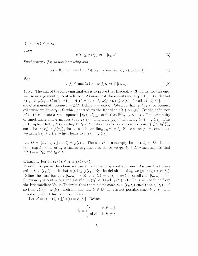
Simulations: Take t0 = 0 and x0 = (0.02,−0.02). It can be observed in Fig. 1 thatlimt→∞ x (t) = 0. Fig. 2 shows that limt→∞ x (t) = 0.

−5 0 5 10 15 20x 10

−3

−0.03

−0.02

−0.01

0

0.01

x1(t)

x 2(t)

(0.02, -0.02)x(0) =

limit point as t ∞

Figure 1: x2(t) versus x1(t) for system (63)-(64).

−0.03 −0.02 −0.01 0−0.06

−0.04

−0.02

0

0.02

0.04

x1(t)

x 2(t

)

starting point at t = 0

limit point as t ∞

Figure 2: x2(t) versus x1(t) for system (63)-(64).

6. Conclusions

This paper dealt with the asymptotic stability of nonlinear time–varying systems. Thestudy is cast within the following framework: given an unknown absolutely continuous

26

function z ≥ 0, provide sufficient conditions on z that allow (1) the knowledge of anupper bound on z and (2) show that z vanishes at infinity. This framework is shown to beuseful for the analysis of the asymptotic stability of some classes of linear and nonlineartime–varying systems.

Acknowledgment

Supported by the Spanish Ministry of Economy, Industry and Competitiveness throughgrant DPI2016-77407-P (AEI/FEDER, UE).

[1] Aeyels, D. & Peuteman, J. (1998) A new asymptotic stability criterion for non-linear time-variant differential equations, IEEE Transactions on Automatic Control,43, 968–971.

[2] Bacciotti, A. & Rosier, L. (2005) Liapunov Functions and Stability in ControlTheory. Springer.

[3] Filippov, A.F. (1988) Differential Equations with Discontinuous Right-Hand Sides.Kluwer.

[4] Khalil, H.K. (2002) Nonlinear Systems. 3rd ed., Prentice Hall, Upper Saddle River,New Jersey, ISBN 0130673897.

[5] Lorıa, A., Panteley, E., Popovic, D. & Teel, A.R. (2005) A nested Ma-trosov theorem and persistency of excitation for uniform convergence in stable nonau-tonomous systems, IEEE Transactions on Automatic Control, 50, 183–198.

[6] Malisoff, M. & Mazenc, F. (2005) Further remarks on strict input-to-statestable Lyapunov functions for time-varying systems, Automatica, 41, 1973–1978.

[7] Mazenc, F. (2003) Strict Lyapunov functions for time-varying systems, Automatica,39, 349–353.

[8] Mu, X. & Cheng, D. (2005) On the stability and stabilization of time-varyingnonlinear control systems, Asian Journal of Control, 7, 244–255.

[9] Naser, M.F.M. & Ikhouane, F. (2013) Consistency of the Duhem model withhysteresis, Mathematical Problems in Engineering, 2013, ID 586130.

[10] Scarciotti, G. & Praly, L. & Astolfi, A. (2016) Invariance-like theorems andweak convergence properties, IEEE Transactions on Automatic Control, 61, 648–661.

27

[11] Schmitt, K. & Thompson, R. (1988) Nonlinear Analysis and Differential Equa-tions: An Introduction, Lecture Notes. University of Utah, Department of Mathe-matics.

[12] Wu, M.Y. (1974) A note on stability of linear time-varying systems, IEEE Trans-actions on Automatic Control, 19, 162.

[13] Yen, E.H. & Van Der Vaart, H.R. (1966) On measurable functions, continuousfunctions and some related concepts, The American Mathematical Monthly, 73, 991–993.

28