Stability of stratified two-phase flows in horizontal channelsI. Barmak, A. Gelfgat, H. Vitoshkin, A. Ullmann, and N. Brauner Citation: Physics of Fluids 28, 044101 (2016); doi: 10.1063/1.4944588 View online: http://dx.doi.org/10.1063/1.4944588 View Table of Contents: http://scitation.aip.org/content/aip/journal/pof2/28/4?ver=pdfcov Published by the AIP Publishing Articles you may be interested in Centrifugal instability of stratified two-phase flow in a curved channel Phys. Fluids 27, 054106 (2015); 10.1063/1.4921631 Eigenspectra and mode coalescence of temporal instability in two-phase channel flow Phys. Fluids 27, 042101 (2015); 10.1063/1.4916404 The impact of deformable interfaces and Poiseuille flow on the thermocapillary instability of threeimmiscible phases confined in a channel Phys. Fluids 25, 024104 (2013); 10.1063/1.4790878 Spatio-temporal linear stability of double-diffusive two-fluid channel flow Phys. Fluids 24, 054103 (2012); 10.1063/1.4718775 Plane Poiseuille flow of a sedimenting suspension of Brownian hard-sphere particles:Hydrodynamic stability and direct numerical simulations Phys. Fluids 18, 054103 (2006); 10.1063/1.2199493

Reuse of AIP Publishing content is subject to the terms at: https://publishing.aip.org/authors/rights-and-permissions. Downloaded to IP: 132.66.194.11

On: Fri, 01 Apr 2016 16:32:02

PHYSICS OF FLUIDS 28, 044101 (2016)

Stability of stratified two-phase flows in horizontalchannels

I. Barmak,a) A. Gelfgat, H. Vitoshkin, A. Ullmann, and N. BraunerSchool of Mechanical Engineering, Tel Aviv University, Tel Aviv 69978, Israel

(Received 17 December 2015; accepted 3 March 2016; published online 1 April 2016)

Linear stability of stratified two-phase flows in horizontal channels to arbitrarywavenumber disturbances is studied. The problem is reduced to Orr-Sommerfeldequations for the stream function disturbances, defined in each sublayer and coupledvia boundary conditions that account also for possible interface deformation andcapillary forces. Applying the Chebyshev collocation method, the equations andinterface boundary conditions are reduced to the generalized eigenvalue problemssolved by standard means of numerical linear algebra for the entire spectrum ofeigenvalues and the associated eigenvectors. Some additional conclusions concern-ing the instability nature are derived from the most unstable perturbation patterns.The results are summarized in the form of stability maps showing the operationalconditions at which a stratified-smooth flow pattern is stable. It is found that forgas-liquid and liquid-liquid systems, the stratified flow with a smooth interface isstable only in confined zone of relatively low flow rates, which is in agreementwith experiments, but is not predicted by long-wave analysis. Depending on the flowconditions, the critical perturbations can originate mainly at the interface (so-called“interfacial modes of instability”) or in the bulk of one of the phases (i.e., “shearmodes”). The present analysis revealed that there is no definite correlation betweenthe type of instability and the perturbation wavelength. C 2016 AIP Publishing LLC.[http://dx.doi.org/10.1063/1.4944588]

I. INTRODUCTION

Stratified flow is a basic flow pattern for gas-liquid and liquid-liquid two-phase flows in a grav-itational field, where the lighter fluid flows above the heavier one. This flow pattern is frequentlyencountered in various important industrial processes. For example, gas-condensate pipelines op-erate primarily in the stratified flow regime. Clearly, the stratified two-phase flow regime can beachieved only for certain ranges of operating conditions for which this flow configuration is stable.Therefore, the knowledge of the stability limits is essential for the design and operation of pipelinesand other process equipment that involve this flow pattern. Instability may result in transition fromstratified-smooth to stratified-wavy flow. Interfacial waves in stratified flow were experimentallyobserved by Charles and Lilleleht (1965) and Yu and Sparrow (1969) and were studied in manyfollowing two-phase flow experimental works (see, e.g., Andritsos and Hanratty, 1987; Tzotzi andAndritsos, 2013; and Birvalski et al., 2014, and references therein). However, growing interfacialdisturbances may lead to transition to other flow patterns (e.g., slug flow, annular flow). Therefore,stability analysis of stratified flow is considered a basic tool to be employed in the modelling of flowpattern transitions and for the prediction of the flow pattern map that is pertinent to the particulartwo-phase flow system of interest.

The exact formulation of transient flow in pipes is too complicated for conducting a rigorousstability analysis. An exact analytical solution for a steady two-phase laminar flow is available inthe literature, where the velocity profiles are in the form of Fourier integrals in a bi-polar coordinate

a)Author to whom correspondence should be addressed. Electronic mail: ilyab@post.tau.ac.il.

1070-6631/2016/28(4)/044101/25/$30.00 28, 044101-1 ©2016 AIP Publishing LLC

Reuse of AIP Publishing content is subject to the terms at: https://publishing.aip.org/authors/rights-and-permissions. Downloaded to IP: 132.66.194.11

On: Fri, 01 Apr 2016 16:32:02

044101-2 Barmak et al. Phys. Fluids 28, 044101 (2016)

system (e.g., Ullmann et al., 2004 and Goldstein et al., 2015). However, a stability analysis requiresa three-dimensional formulation and results in a too complicated problem. Therefore, a commonapproach is to use a transient one dimensional Two-Fluid (TF) mechanistic model for the stabilityanalysis. Early studies on the stability of stratified gas-liquid flow in pipes assumed inviscid flowand considered only the transient momentum equation of the gas phase, ignoring the dynamics ofthe liquid phase (e.g., Kordyban and Ranov, 1970; Wallis and Dobson, 1973; Taitel and Dukler,1976; and Mishima and Ishii, 1980). Obviously, the prediction of the stratified flow boundary for ageneral two-phase system requires consideration of the inertia and viscous effects of both phases.A more rigorous approach that was followed in many later studies is to consider viscid flow and touse the 1D transient continuity and momentum equations of the two phases (e.g., Lin and Hanratty,1986; Wu et al., 1987; Andritsos et al., 1989; Brauner and Moalem Maron, 1991; 1993; and Barneaand Taitel, 1994). However, the predictions obtained via the two-fluid model critically dependon the reliability of the closure relations used to model the base flow and the interaction of thebase flow with the interfacial disturbance (e.g., steady and wave induced wall and interfacial shearstresses, velocity profile shape factors, see Kushnir et al., 2007; 2014). Moreover, the stability anal-ysis is restricted to long-wave perturbations, since long-wave perturbation is an inherent assumptionwhen the two-fluid model is used.

An alternative approach is to conduct a rigorous stability analysis of a two-layer plane Poiseuilleflow (i.e., Two Plates (TP) geometry), while considering all wave number perturbations in order toobtain insight into the mechanisms involved in the destabilization of stratified flow. Such a formulationallows for the Squire transformation (Hesla et al., 1986), so that only two-dimensional disturbancescan be considered. In this approach, two types of instability are considered: shear-flow instabilityand interfacial instability. Shear-flow instability is due to the interaction of the flow with the channelwalls (encountered also in single-phase Poiseuille flow, i.e., Tollmien-Schlichting waves), whichleads to transition to turbulent flow in either of the phases for sufficiently large Reynolds number.This type of instability is commonly associated with short-wave instability. Interfacial instability isdue to the interaction between the fluids at the interface, which results from energy transfer fromthe main flow to interfacial disturbances. In this case the instability is attributed to viscosity and/ordensity stratification (jump) and is commonly associated with (relatively) long-wave instability.

Boomkamp and Miesen (1996) offered a classification of ways of energy transfer from the baseto the disturbed flow. According to that study, there are five different mechanisms by which energytransfer can be conducted. Each mechanism has its origins in one of the following flow features:density stratification, velocity profile curvature, viscosity stratification, shear effects, or a combina-tion of viscosity stratification and shear effects. The stability analysis of stratified two-phase flowremains rather complicated even in the simpler two-plate geometry due to the multiplicity of thedimensionless parameters involved. Consequently, the studies conducted were usually limited to anarrow parameter range (e.g., Boomkamp and Miesen, 1996). A brief review on the history andmost important results obtained for the considered problem are given below.

The linear stability of stratified plane horizontal Poiseuille flow of two superposed fluidswith different viscosities was first studied theoretically in the classic work of Yih (1967), wherelong-wave two-dimensional analysis was carried out. It was shown that the viscosity stratificationalone can cause interfacial instability for an arbitrary low Reynolds number, when the fluids occupyequal volumes in the channel. Yih introduced the concept of an interfacial mode, which can coin-cide with any streamline and is neutrally stable in single-fluid flow but triggers instability whenviscosity stratification exists.

The interface may be unstable also to short-wavelength perturbations as was shown by Hooperand Boyd (1983). For the case of equal densities and zero surface tension, they obtained exactdispersion relation for disturbances of arbitrary wavelength. Taking an unbounded Couette flow oftwo fluids of different viscosities as an example, it was shown additionally that presence of rigidboundaries does not play an essential role in the flow instability (in contrast to the case of planePoiseuille flow of a homogeneous fluid). It was also demonstrated that the effect of surface tensionis always stabilizing, whereas a density difference may have either stabilizing or destabilizing effect.

The numerical study of Yiantsios and Higgins (1988) accounted for density stratification,different fluid layers’ thicknesses, the effects of interfacial tension and gravity. They showed that

Reuse of AIP Publishing content is subject to the terms at: https://publishing.aip.org/authors/rights-and-permissions. Downloaded to IP: 132.66.194.11

On: Fri, 01 Apr 2016 16:32:02

044101-3 Barmak et al. Phys. Fluids 28, 044101 (2016)

a shear perturbation mode, which is essentially a short-wavelength disturbance of the Tollmien-Schlichting type, modified by the interfacial effects, can destabilize stratified flow at sufficientlylarge Reynolds numbers. For the single fluid case, the shear mode originated at the channel walls isthe only source of instabilities, but two-phase flow may be unstable to more than one mode. Tilleyet al. (1994) extended the study of Yiantsios and Higgins (1988). They studied the influence ofthe channel height and the (heavy) layer thickness on the flow stability in horizontal and inclinedchannels. Their analysis of the dominant unstable modes demonstrates the qualitative differencesbetween single- and two-layer systems. The effect of inclination was further studied by Vempatiet al. (2010), but they paid a limited attention to horizontal flows. The most recent paper on the topicof linear instability in two-phase horizontal flow was published by Kaffel and Riaz (2015). Theyfocused on spectral characteristics and eigenfunction patterns (amplitude of the stream functionperturbation) related to shear and interfacial modes of instability and the interaction between themin the unstable region.

The above studies contribute to the understanding of the nature of instability and the mainmechanisms that are responsible for the flow destabilization. However, the analyses conducted inthose studies were not used to obtain physical interpretations that may lead to improvement of themodelling of flow pattern transitions.

In this study, the linear stability of stratified two-phase flows in horizontal channels with respectto arbitrary wavenumber disturbances is explored. Temporal disturbances are considered, so thatthe mathematical problem reduces to solution of a series of generalized eigenvalue problems. Forthe sake of further physical interpretations and practical applications, this rigorous analysis toolis applied for predicting the stability boundaries on the flow pattern maps of particular gas-liquidand liquid-liquid systems, thus extending previous results of long-wave analysis by Kushnir et al.(2014). The critical disturbances that are responsible for triggering the instability (i.e., the mostunstable disturbance mode) are identified. For characterization of the instability mode associatedwith the critical disturbances two-dimensional contours of the stream function and the amplitude ofthe velocity perturbations are examined. The obtained results offer a better physical insight into thephenomenon of two-phase flow instability and may help to improve the modelling of flow patterntransitions, which are usually based on the simplified 1D transient two-fluid models.

II. PROBLEM FORMULATION

We consider a stratified two-layer flow of two immiscible incompressible fluids in a horizontalchannel (i.e., zero angle of inclination from the horizontal, β = 0◦). The flow is assumed to beisothermal and is driven by an imposed pressure gradient. The flow configuration is sketched inFigure 1. The interface between the fluids, labeled as j = 1,2 (1—lower phase, 2—upper phase), isassumed to be flat in the undisturbed base flow state. Under this assumption, the model allows fora plane-parallel solution, in which position of the interface is an unknown value (to be determinedbelow).

The flow in each liquid is described by the continuity and momentum equations that arerendered dimensionless (see Kushnir et al., 2014), choosing for the scales of length and velocity the

FIG. 1. Configuration of stratified two-layer flow in a horizontal channel.

Reuse of AIP Publishing content is subject to the terms at: https://publishing.aip.org/authors/rights-and-permissions. Downloaded to IP: 132.66.194.11

On: Fri, 01 Apr 2016 16:32:02

044101-4 Barmak et al. Phys. Fluids 28, 044101 (2016)

height of the upper layer h2 and the interfacial velocity ui, respectively. The time and the pressureare scaled by h2/ui and ρ2u2

i , respectively. The dimensionless continuity and momentum equationsare

div u j = 0,∂u j

∂t+

�u j · ∇

�u j = −

ρ1

r ρ j∇pj +

1Re2

ρ1

r ρ j

mµ j

µ1∆u j −

1Fr2

ey,(1)

where u j =�u j, v j

�and pj are the velocity and pressure of the fluid j, ρ j and µ j are the corre-

sponding density and dynamic viscosity, and ey is the unit vector in the direction of the y-axis (thedirection of gravity).

In the dimensionless formulation the lower and upper phases occupy the regions −n ≤ y ≤ 0and 0 ≤ y ≤ 1, respectively, where n = h1/h2. Other dimensionless parameters: Re2 = ρ2uih2/µ2 isthe Reynolds number, Fr2 = u2

i/gh2 is the Froude number, and r = ρ1/ρ2 and m = µ1/µ2 are thedensity and viscosity ratios. Since the horizontal two-phase flow allows for the Squire transforma-tion (Hesla et al., 1986), we assume that most unstable disturbances are two-dimensional and shouldtherefore be considered in the stability analysis.

The velocities satisfy the no-slip boundary conditions at the channel walls

u1 (y = −n) = 0, u2 (y = 1) = 0. (2)

Boundary conditions at the interface y = η (x, t) require continuity of velocity components andthe tangential stresses, and jump of the normal stress due to the surface tension (the square bracketsdenote the jump of expression value across the interface)

u1 (y = 0) = u2 (y = 0) , (3)

[t · T · n] =

mµµ1

(∂u∂ y+∂v

∂x

)*,1 −

(∂η

∂x

)2+-− 4

∂u∂x

∂η

∂x

= 0, (4)

[n · T · n] =p +

mµµ1

2Re−12

1 +(∂η∂x

)2*,

∂u∂x

*,1 −

(∂η

∂x

)2+-+

(∂u∂ y+∂v

∂x

)∂η

∂x+-

=We−12

∂2η

∂x2(1 +

(∂η∂x

)2)3/2 ,

(5)

where n is the unit normal vector pointing from lower into upper phase, t is the unit vector tangentto the interface, T is the stress tensor. An additional dimensionless parameter We2 = ρ2h2u2

i/σ is theWeber number, and σ is the surface tension coefficient.

Additionally, the interface displacement and the normal velocity components at the interfacesatisfy the kinematic boundary condition

v j =DηDt=∂η

∂t+ u j

∂η

∂x. (6)

III. THE BASE FLOW

The base flow is assumed to be steady, laminar, and fully developed. Assuming that the hori-zontal velocity U (y) varies only with the vertical coordinate, y , the exact steady-state solution forthe (dimensionless) velocity profiles reads (e.g., Ullmann et al., 2003 and Kushnir et al., 2014)

U1 = 1 + a1y + b1y2 for − n ≤ y ≤ 0, U2 = 1 + a2y + b2y

2 for 0 ≤ y ≤ 1, (7)

where

a1 =a2

m, a2 =

m − n2

n2 + n, b1 = −

m + n(n2 + n)m

, b2 = −m + nn2 + n

.

To apply collocation method based on the Chebyshev polynomials (defined in the interval[0, 1]), we introduce a new coordinate y1 = (y + n) /n, whereby 0 ≤ y1 ≤ 1 for the part of the

Reuse of AIP Publishing content is subject to the terms at: https://publishing.aip.org/authors/rights-and-permissions. Downloaded to IP: 132.66.194.11

On: Fri, 01 Apr 2016 16:32:02

044101-5 Barmak et al. Phys. Fluids 28, 044101 (2016)

channel occupied by the lower phase, and y2 = y, 0 ≤ y2 ≤ 1 for the upper phase (which remainsunchanged). After substitution of the new coordinate, the velocity profile in the lower phase reads

U1 = 1 + a1y + b1y2 = 1 + a1 (y1 − 1) n + b1(y1 − 1)2 n2

= 1 − a1n + b1n2 c1

+�a1n − 2b1n2�

a1

y1 + b1n2b1

y21 . (8)

It is convenient to use the lower (heavy) phase holdup, h = h1/H , instead of thickness ration = h1/h2. The heavy phase holdup can be found by solving the following algebraic equation,F (q,m,h) = 0 (e.g., Ullmann et al., 2003):

mq(1 − h)2 [(1 + 2h)m + (1 − m) h (4 − h)] − h2 �(3 − 2h)m + (1 − m) h2�

4h3(1 − h)3 [h + m (1 − h)] = 0. (9)

Equation (9) can be represented as a 4th order algebraic equation in h, using the Martinelli param-eter X2 =

(−dP/dx)1S(−dP/dx)2S = m · q,

�X2 + 1

� (m − 1) h4 + 2X2 (3 − 2m) h3 +�3X2 (2m − 3) − 3m

�h2

+4X2 (1 − m) h + X2m = 0.(10)

Thus, the primary flow solution for horizontal flow is fully determined by two dimensionlessparameters, the viscosity ratio m = µ1/µ2 and the flow rate ratio q = q1/q2. Here qj is the feedflow rate of phase j and (−dP/dx) jS = 12µ jqj/H3 is the corresponding superficial pressure dropof phase j (i.e., when flowing alone in the channel of height H = h1 + h2). Another importantcharacteristic of the flow—the dimensionless pressure drop can be calculated as

P =dP/dx

(−dP/dx)2S =3mq(1 − h)2 − 4mh (1 − h) − h2

4h(1 − h)2 [(1 + 2h)m + (1 − m) h (4 − h) − 3h] . (11)

The interfacial velocity can also be found

ui =ui

U2S=

6h (1 − h) �−P

�

m (1 − h) + h, (12)

where U2S = q2/H is the superficial velocity of the upper phase.Henceforth, we use the superficial velocity and the flow rate concepts interchangeable due to

consideration of channels of constant height.

IV. LINEAR STABILITY ANALYSIS

In the following we study linear stability of above plane-parallel solution with respect to infin-itesimal, two-dimensional disturbances. The perturbed velocities and pressure fields are writtenas u j = Uj + u j, v j = v j , pj = Pj + pj, and η = η for the dimensionless disturbance of the inter-face. The disturbed velocities are conveniently represented by the corresponding stream function�u j = ∂ψ j/∂ y ; v j = −∂ψ j/∂x

�, and an exponential dependence of the perturbation in time is

assumed

*...,

ψ j

pj

η

+///-

=*...,

φ j (y)f j (y)Hη

+///-

e(ikx+λt) , *,

u j

v j+-= *

,

φ′j−ikφ j

+-

e(ikx+λt), (13)

where φ j, f j, and Hη are the perturbation amplitudes, k is the dimensionless real wavenumber(k = 2πh2/lwave, with lwave being the wavelength), and λ is the complex time increment. Aftersubstitution and linearization of the original equations and boundary conditions (1)-(6), the problemis reduced to the Orr-Sommerfeld equations, written here in the eigenvalue problem form

0 ≤ y1 ≤ 1 : λD1φ1 =

ik

(−U1D1 +

U ′′1n2

)+

1Re1

D21

φ1, (14)

Reuse of AIP Publishing content is subject to the terms at: https://publishing.aip.org/authors/rights-and-permissions. Downloaded to IP: 132.66.194.11

On: Fri, 01 Apr 2016 16:32:02

044101-6 Barmak et al. Phys. Fluids 28, 044101 (2016)

0 ≤ y2 ≤ 1 : λDφ2 =

ik

�−U2D +U ′′2

�+

1Re2

D2φ2, (15)

where

Dφ = φ′′ − k2φ, D2φ = φIV − 2k2φ′′ + k4φ,

D1φ =φ′′

n2 − k2φ, D21φ =

φIV

n4 − 2k2φ′′

n2 + k4φ.(16)

The linearized boundary conditions are obtained by means of Taylor expansions of η around itsunperturbed zero value (see Segal, 2008, for more details)

y1 = 1, y2 = 0 : λHη = −ik�φ2 +U2Hη

�, (17)

where

Hη =φ′2 (0) − φ′1 (1) /nU ′1 (1) /n −U ′2 (0)

,

y1 = 1, y2 = 0 : λ

(r ·

φ′1 (1)n− φ′2 (0)

)= ik

−

(k2We−1

2 +(r − 1)

Fr2

)· Hη

+ r(−U1

φ′1 (1)n+

U ′1 (1)n

φ1 (1))+

�U2φ

′2 (0) −U ′2 (0) φ2 (0)�

+1

Re2

m

(φ′′′1 (1)

n3 − 3k2φ′1 (1)n

)−

�φ′′′2 (0) − 3k2φ′2 (0)

�,

(18)

y1 = 0 (y = −n) , φ1 = φ′1 = 0, (19)

y2 = 1, φ2 = φ′2 = 0, (20)

y1 = 1, y2 = 0 : φ1 (1) = φ2 (0) , (21)

y1 = 1, y2 = 0 : mφ′′1 (1)

n2 + k2φ1 (1) +U ′′1n2 Hη

= φ′′2 (0) + k2φ2 (0) +U ′′2 Hη. (22)

Note that the third terms on both sides of Equation (22) are equal in case of horizontal flow andcancel out.

The temporal linear stability is studied by solving the system of differential system (14), (15),and (17)-(22) assuming an arbitrary wavenumber for each given set of the other parameters. Defin-ing the time increment as a complex eigenvalue λ = λR + iλ I , we note that λR determines thegrowth rate of perturbation. The flow is unstable when at least one of the λR’s is positive. Neutralstability corresponds to max(λR) = 0. The flow is considered to be stable, when real parts of allthe eigenvalues are negative. The phase speed of the perturbation is −λ I/k, where λ I is the waveangular frequency.

V. NUMERICAL METHOD

Following several previous studies, the Chebyshev collocation method is used to discretize theOrr-Sommerfeld equations and the boundary conditions. This numerical method uses Chebyshevpolynomials to approximate the solution in each sublayer as a truncated Chebyshev series

φ( j) =Ni=1

d( j)i Ti(y), (23)

where j = 1,2—phase index, d( j)i —unknown coefficients, Ti (y)—shifted Chebyshev polynomials

of the ith degree over the interval 0 ≤ y ≤ 1. The equations are evaluated at the roots of theChebyshev polynomial of N-th order (collocation points), reducing the differential problem to thegeneralized eigenvalue problem

λ · A · d = B · d, (24)

Reuse of AIP Publishing content is subject to the terms at: https://publishing.aip.org/authors/rights-and-permissions. Downloaded to IP: 132.66.194.11

On: Fri, 01 Apr 2016 16:32:02

044101-7 Barmak et al. Phys. Fluids 28, 044101 (2016)

TABLE I. Comparison of the present numerical results and asymptotic solution of Kushnir et al. (2014) for the criticalsuperficial velocities. Calculation with N= 50.

U1S, m/s

Horizontal channel H = 0.02 m U2S, m/s Asymptotic Numerical

Air-water flow r = 1000 m = 55

5 0.016 332 91 0.016 324 12.5 0.031 049 10 0.031 042 040.25 0.052 283 60 0.052 272 380.15 0.882 701 24 0.882 661 23

Liquid-liquid flow r = 1.25 m = 0.5

0.001 0.149 875 68 0.149 856 470.05 0.289 904 55 0.289 845 580.3 0.286 238 71 0.286 228 81 0.731 312 43 0.731 354 26

where the matrices order is of 2N + 1. The eigenvalue problem is solved by the QR algorithm(Francis, 1962). Accurate numerical results were compared with the long-wave asymptotic solutionof Kushnir et al. (2014) (see Table I). The numerical convergence of the method was verifiedseparately and is illustrated in Table II.

Most of the results below are computed using the truncation number N = 50, that according toTable II yields 6 correct decimal digits of the critical superficial velocity.

VI. RESULTS AND DISCUSSION

All wavelength linear stability analysis of horizontal liquid-liquid and gas-liquid flows wascarried out to study stability limits of stratified flows and to reveal the destabilization mechanismsinvolved. Although the base flow characteristics are determined by only two dimensionless param-eters (m, q), five parameters, i.e., m, q, r, Re2S, or Fr2S, and We2s govern the linear stability of thebase flow and its further non-linear evolution. Here Rejs = ρ jUj sH/µ j and Frjs = U2

j s/ (gH) are thesuperficial Reynolds and Froude numbers, respectively, and Wejs = ρ jU2

jsH/σ is the Weber num-ber. The large number of parameters makes the overall parametric analysis practically unfeasible.Therefore, in the present work, we set the values of the physical properties at several representativeexamples and study the stability of the flow by varying flow rates in each fluid layer. In all cases theupper layer is considered to be lighter than the lower layer, so that the Rayleigh-Taylor instability isnot encountered. Along with presenting the all wavelength stability boundaries, we are interested incomparison with the analytical results obtained for the long-wave limit. The most unstable pertur-bations described by the leading eigenfunctions are also reported and their patterns are discussed,which allows arriving at additional conclusions on the nature of instability.

There are several mechanisms, which can be responsible for destabilization of the flat inter-face solution. One of them is a shear flow instability, which is encountered also in single-phase

TABLE II. Convergence of the critical superficial velocity of the heavy phase U1s with the increase of truncationnumber N.

Horizontal air-water flow:H = 0.02 m, r = 1000, m = 55, σ = 0.072 N/m

Order of Chebyshev polynomials, N U2S = 0.25 m/s, k = 10−5 U2S = 2 m/s, k = 3

25 1.705 142 6 0.010 672 38750 1.705 113 5 0.010 611 21875 1.705 113 4 0.010 611 217100 1.705 113 4 0.010 611 217

Reuse of AIP Publishing content is subject to the terms at: https://publishing.aip.org/authors/rights-and-permissions. Downloaded to IP: 132.66.194.11

On: Fri, 01 Apr 2016 16:32:02

044101-8 Barmak et al. Phys. Fluids 28, 044101 (2016)

Poiseuille flow and leads to transition to turbulent flow for Reynolds numbers higher than critical.This instability originates near the channel walls and is related to amplification of short wave-length Tollmien-Schlichting waves in either of the phases. The presence of this instability modealready proves that the long-wave analysis is insufficient for determining the stability boundaries ofstratified two-phase flow.

In two-phase flow it may occur that instability originates at the interface and is associated withviscosity and/or density stratification (e.g., Yih, 1967 and Kushnir et al., 2014). Such instabilityis viewed as a result of interaction of the flows in the two layers, which are connected throughthe velocity and viscous stresses boundary conditions at the interface (Tilley, 1994). As a result,the flow can become unstable for lower flow rates (lower superficial Reynolds number) than inplane Poiseuille flow. Viscosity stratification (m , 1) produces a discontinuity (jump) across theinterface in the primary flow velocity gradient U ′j, which leads to energy transfer from the primaryflow to the disturbed flow and causes the “viscosity induced” instability. According to Hooper andBoyd (1983) and Boomkamp and Miesen (1996), this is the dominant mechanism for the so-called“interfacial instability.” It should be emphasized that since the stability problem is linear, severalindependent destabilizing mechanisms may be observed, which will appear as distinct unstableeigenfunctions.

A. Liquid-liquid systems

First, we consider two liquid-liquid systems with different viscosity ratios and with identicaldensity ratios and channel heights. The stability map for horizontal flow with a more viscous(m = 0.5) light phase (oil) is shown in Figure 2. The surface tension is neglected. The stabilitymap is plotted for dimensional superficial velocities, for the channel of 2 cm height, the oil densityand dynamic viscosity are ρ2 = 800 kg/m3 and µ2 = 0.0005 Pa s, respectively. In the frameworkof long the long-wave analysis (black dashed line in Figure 2) this flow is shown to be stablefor any upper (light and more viscous) phase flow rate, provided the flow rate of the heavy (lessviscous) phase is sufficiently low (for details see Kushnir et al., 2014). According to the long-waveanalysis, at low oil superficial velocities there exists a critical heavy phase superficial velocitythat depends on density ratio between phases and flow rate of light phase (black dashed line inFigure 2). In the region of large flow rates of both phases, when viscosity effects surpass theeffect of gravity, the long-wave stability boundary approaches the zero-gravity stability boundary(see Kushnir et al., 2014). This behavior of the long-wave stability boundary is common for all

FIG. 2. Stability boundary for horizontal liquid-liquid flow without surface tension (We→ ∞), the light phase is more viscous�m = 0.5; ρ2= 800 kg/m3; µ2= 5 ·10−4 Pa s

�.

Reuse of AIP Publishing content is subject to the terms at: https://publishing.aip.org/authors/rights-and-permissions. Downloaded to IP: 132.66.194.11

On: Fri, 01 Apr 2016 16:32:02

044101-9 Barmak et al. Phys. Fluids 28, 044101 (2016)

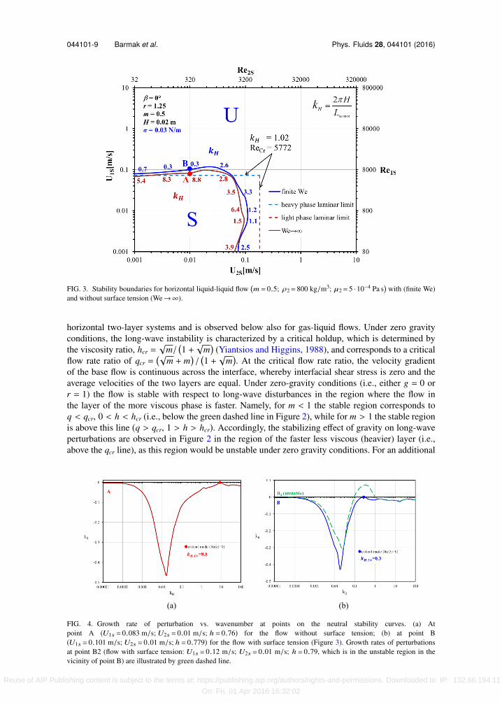
FIG. 3. Stability boundaries for horizontal liquid-liquid flow�m = 0.5; ρ2= 800 kg/m3; µ2= 5 ·10−4 Pa s

�with (finite We)

and without surface tension (We→ ∞).

horizontal two-layer systems and is observed below also for gas-liquid flows. Under zero gravityconditions, the long-wave instability is characterized by a critical holdup, which is determined bythe viscosity ratio, hcr =

√m/

�1 +√

m�

(Yiantsios and Higgins, 1988), and corresponds to a criticalflow rate ratio of qcr =

�√m + m

�/

�1 +√

m�. At the critical flow rate ratio, the velocity gradient

of the base flow is continuous across the interface, whereby interfacial shear stress is zero and theaverage velocities of the two layers are equal. Under zero-gravity conditions (i.e., either g = 0 orr = 1) the flow is stable with respect to long-wave disturbances in the region where the flow inthe layer of the more viscous phase is faster. Namely, for m < 1 the stable region corresponds toq < qcr, 0 < h < hcr (i.e., below the green dashed line in Figure 2), while for m > 1 the stable regionis above this line (q > qcr, 1 > h > hcr). Accordingly, the stabilizing effect of gravity on long-waveperturbations are observed in Figure 2 in the region of the faster less viscous (heavier) layer (i.e.,above the qcr line), as this region would be unstable under zero gravity conditions. For an additional

FIG. 4. Growth rate of perturbation vs. wavenumber at points on the neutral stability curves. (a) Atpoint A (U1s = 0.083 m/s; U2s = 0.01 m/s; h = 0.76) for the flow without surface tension; (b) at point B(U1s = 0.101 m/s; U2s = 0.01 m/s; h = 0.779) for the flow with surface tension (Figure 3). Growth rates of perturbationsat point B2 (flow with surface tension: U1s = 0.12 m/s; U2s = 0.01 m/s; h = 0.79, which is in the unstable region in thevicinity of point B) are illustrated by green dashed line.

Reuse of AIP Publishing content is subject to the terms at: https://publishing.aip.org/authors/rights-and-permissions. Downloaded to IP: 132.66.194.11

On: Fri, 01 Apr 2016 16:32:02

044101-10 Barmak et al. Phys. Fluids 28, 044101 (2016)

verification of the numerical results we calculated the stability boundary for k → 0 (blue squares),which successfully compare with the analytical results for the long-wave instability (black dashedline).

Considering perturbations of all possible wavelengths, we obtain different results. The flowis stable only in a bounded region of the phases flow rates (within the red curve in Figure 2),which is much smaller than that obtained by the long-wave approach. This observation meansthat intermediate and short-wave disturbances are amplified stronger for lower flow rates than thelong waves. More details can be seen in Figures 3 and 4. Figure 3 presents stability diagrams forzero and non-zero surface tensions including also the critical wavenumbers (normalized by thechannel height, kH = 2πH/lwave) for both cases. Figure 4 presents two examples of the growth ratedependence on the wavenumber (at points A and B in Figure 3).

Comparing instabilities at low U2S for finite and infinite Weber numbers, we see that at zerosurface tension (We → ∞) the critical mode wavenumber is considerably larger than unity, indicat-ing short-wave instability. Including a realistic surface tension in the model (finite We) we expecta stabilization effect, since it becomes more difficult to perturb the interface. Obviously, the sur-face tension suppresses short-wave perturbations and leaves the long waves almost unaffected. Astabilization effect of the surface tension is indeed observed (Figure 3), however, its effect on thecritical oil and water superficial velocities is rather moderate. The main effect of the surface tensionis on the wavenumber of the critical perturbation. As surface tension stabilizes the short waves, thecritical perturbation is shifted to lower wavenumber, i.e., longer waves are responsible for triggeringinstability. This is demonstrated in Figure 4, where the growth rate of the perturbations vs. thewavenumber at points A and B are compared. As demonstrated in Figures 4(b), a slight increaseof the superficial velocity of one of the phases beyond the critical conditions (i.e., in the unstableregion), results in positive values of the growth rate of perturbations in a range of wavenumbersaround the critical one, indicating flow instability.

Single phase limits for laminar flow of light phase and laminar flow of heavy phase are plottedin Figure 3. When oil flow rate tends to zero, the neutral stability curve approaches the single phaselimit for water flow determined by the critical Reynolds number (ReCr = 5772, critical wavenumberkH = 1.02 (e.g., Orszag, 1971)). The wavenumber of the most unstable mode also tends to that ofsingle phase flow. Therefore, it can be concluded that this is a shear mode of instability, which is

FIG. 5. Stability map for horizontal oil-water flow�m = 2; ρ2= 800 kg/m3; µ2= 5 ·10−4 Pa s

�with (finite We) and without

surface tension (We→ ∞).

Reuse of AIP Publishing content is subject to the terms at: https://publishing.aip.org/authors/rights-and-permissions. Downloaded to IP: 132.66.194.11

On: Fri, 01 Apr 2016 16:32:02

044101-11 Barmak et al. Phys. Fluids 28, 044101 (2016)

associated with the short wavelength Tollmien-Schlichting wave, modified by the presence of theinterface. The introduction of a thin layer of oil (small holdup) to the (single phase) water flow has astabilizing effect. On the other hand, if a thin heavy layer of water is added to the (single phase) oilflow, a destabilizing effect is observed.

The stability map for horizontal oil-water flow with a less viscous (m = 2) light phase�oil : ρ2 = 800 kg/m3, µ2 = 0.0005 Pa s, µ1 = 0.001 Pa s

�is shown in Figure 5. In accordance

with the discussion above (with reference to Figure 2), when long-wave perturbations are consid-ered (k → 0), the region where the water layer is faster would be stable under zero gravity condi-tions (i.e., above the qcr line). In this case, the stabilizing effects of gravity are observed in the regionwhere the oil (less viscous) layer is faster. Accordingly, the flow is stable in an unbounded region oflarge holdups of water (low oil flow rates) and is limited only by the flow rates of the less viscous oilphase. However, owing to the short wavelength perturbations, the flow is stable only in a boundedrange of the water (more viscous phase) flow rates, and also in a reduced range the oil flow rates.The neutral stability curve in this case looks similar to what was observed in the flow with inverseviscosity ratio m = 0.5. The stabilizing effect of the surface tension (expansion of stable region) issignificant only in the region of similar flow rates (holdups) of the two phases. It can be concludedthat in oil-water flows the effect of surface tension on the stable region is rather moderate.

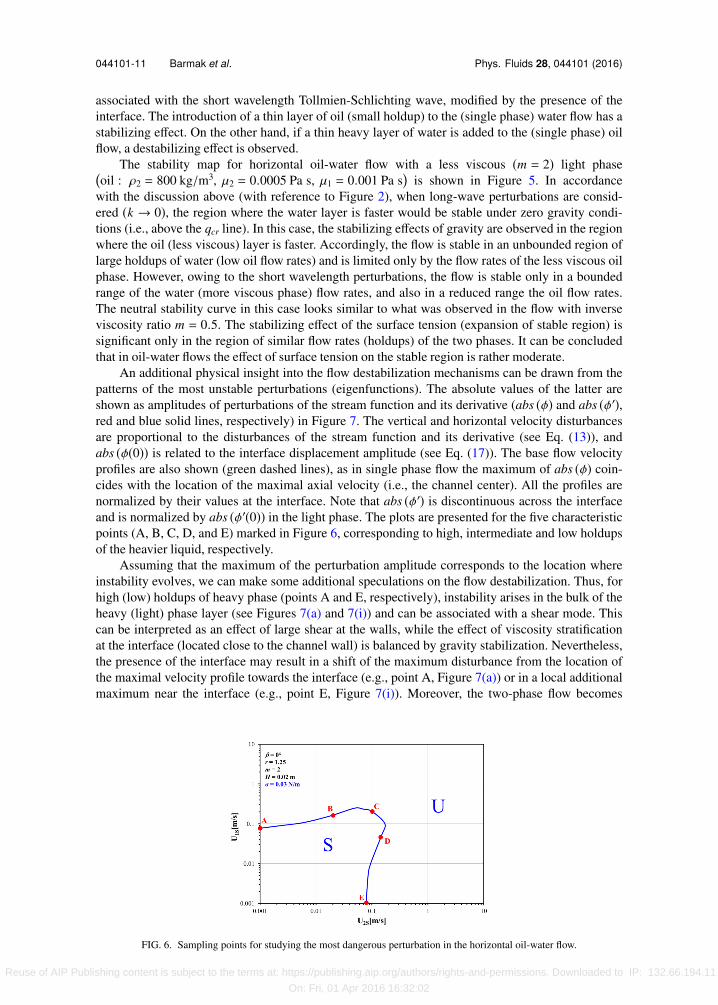
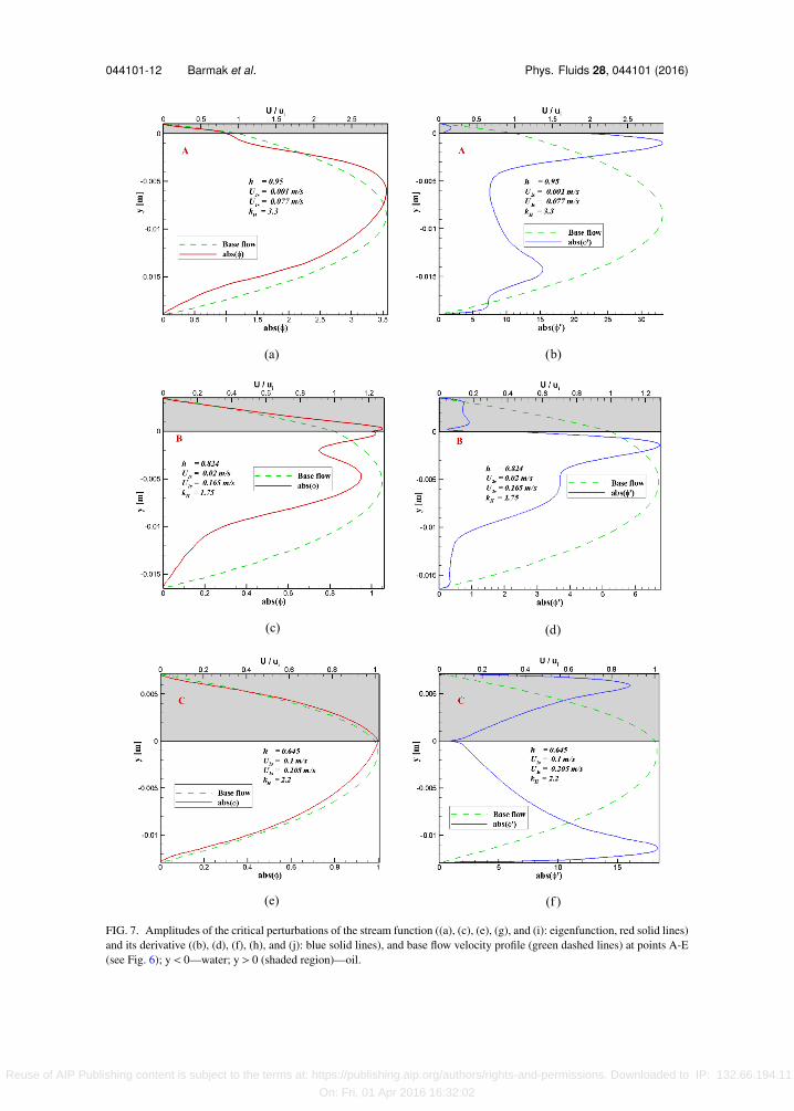
An additional physical insight into the flow destabilization mechanisms can be drawn from thepatterns of the most unstable perturbations (eigenfunctions). The absolute values of the latter areshown as amplitudes of perturbations of the stream function and its derivative (abs (φ) and abs (φ′),red and blue solid lines, respectively) in Figure 7. The vertical and horizontal velocity disturbancesare proportional to the disturbances of the stream function and its derivative (see Eq. (13)), andabs (φ(0)) is related to the interface displacement amplitude (see Eq. (17)). The base flow velocityprofiles are also shown (green dashed lines), as in single phase flow the maximum of abs (φ) coin-cides with the location of the maximal axial velocity (i.e., the channel center). All the profiles arenormalized by their values at the interface. Note that abs (φ′) is discontinuous across the interfaceand is normalized by abs (φ′(0)) in the light phase. The plots are presented for the five characteristicpoints (A, B, C, D, and E) marked in Figure 6, corresponding to high, intermediate and low holdupsof the heavier liquid, respectively.

Assuming that the maximum of the perturbation amplitude corresponds to the location whereinstability evolves, we can make some additional speculations on the flow destabilization. Thus, forhigh (low) holdups of heavy phase (points A and E, respectively), instability arises in the bulk of theheavy (light) phase layer (see Figures 7(a) and 7(i)) and can be associated with a shear mode. Thiscan be interpreted as an effect of large shear at the walls, while the effect of viscosity stratificationat the interface (located close to the channel wall) is balanced by gravity stabilization. Nevertheless,the presence of the interface may result in a shift of the maximum disturbance from the location ofthe maximal velocity profile towards the interface (e.g., point A, Figure 7(a)) or in a local additionalmaximum near the interface (e.g., point E, Figure 7(i)). Moreover, the two-phase flow becomes

FIG. 6. Sampling points for studying the most dangerous perturbation in the horizontal oil-water flow.

Reuse of AIP Publishing content is subject to the terms at: https://publishing.aip.org/authors/rights-and-permissions. Downloaded to IP: 132.66.194.11

On: Fri, 01 Apr 2016 16:32:02

044101-12 Barmak et al. Phys. Fluids 28, 044101 (2016)

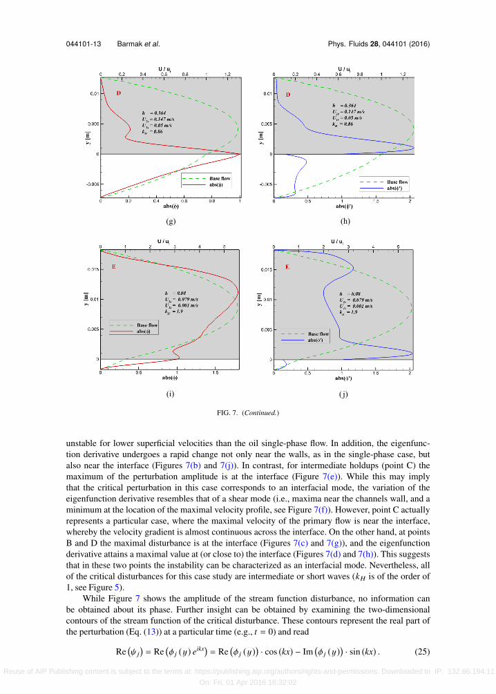
FIG. 7. Amplitudes of the critical perturbations of the stream function ((a), (c), (e), (g), and (i): eigenfunction, red solid lines)and its derivative ((b), (d), (f), (h), and (j): blue solid lines), and base flow velocity profile (green dashed lines) at points A-E(see Fig. 6); y < 0—water; y > 0 (shaded region)—oil.

Reuse of AIP Publishing content is subject to the terms at: https://publishing.aip.org/authors/rights-and-permissions. Downloaded to IP: 132.66.194.11

On: Fri, 01 Apr 2016 16:32:02

044101-13 Barmak et al. Phys. Fluids 28, 044101 (2016)

FIG. 7. (Continued.)

unstable for lower superficial velocities than the oil single-phase flow. In addition, the eigenfunc-tion derivative undergoes a rapid change not only near the walls, as in the single-phase case, butalso near the interface (Figures 7(b) and 7(j)). In contrast, for intermediate holdups (point C) themaximum of the perturbation amplitude is at the interface (Figure 7(e)). While this may implythat the critical perturbation in this case corresponds to an interfacial mode, the variation of theeigenfunction derivative resembles that of a shear mode (i.e., maxima near the channels wall, and aminimum at the location of the maximal velocity profile, see Figure 7(f)). However, point C actuallyrepresents a particular case, where the maximal velocity of the primary flow is near the interface,whereby the velocity gradient is almost continuous across the interface. On the other hand, at pointsB and D the maximal disturbance is at the interface (Figures 7(c) and 7(g)), and the eigenfunctionderivative attains a maximal value at (or close to) the interface (Figures 7(d) and 7(h)). This suggeststhat in these two points the instability can be characterized as an interfacial mode. Nevertheless, allof the critical disturbances for this case study are intermediate or short waves (kH is of the order of1, see Figure 5).

While Figure 7 shows the amplitude of the stream function disturbance, no information canbe obtained about its phase. Further insight can be obtained by examining the two-dimensionalcontours of the stream function of the critical disturbance. These contours represent the real part ofthe perturbation (Eq. (13)) at a particular time (e.g., t = 0) and read

Re�ψ j

�= Re

�φ j (y) eikx�

= Re�φ j (y)� · cos (kx) − Im

�φ j (y)� · sin (kx) . (25)

Reuse of AIP Publishing content is subject to the terms at: https://publishing.aip.org/authors/rights-and-permissions. Downloaded to IP: 132.66.194.11

On: Fri, 01 Apr 2016 16:32:02

044101-14 Barmak et al. Phys. Fluids 28, 044101 (2016)

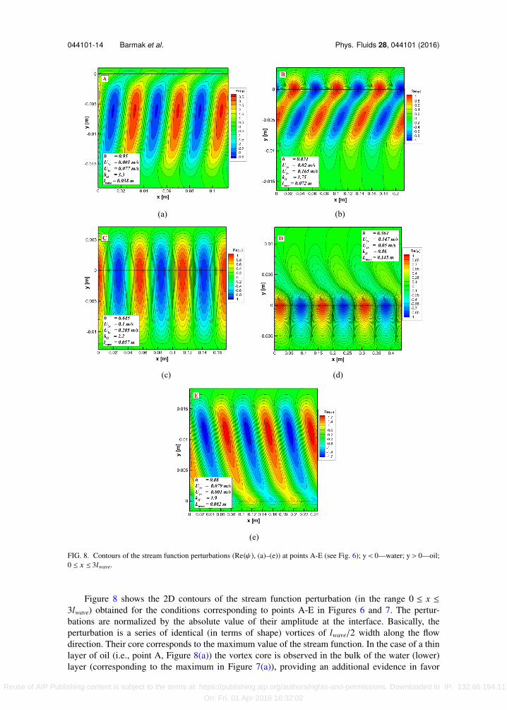
FIG. 8. Contours of the stream function perturbations (Re(ψ), (a)–(e)) at points A-E (see Fig. 6); y < 0—water; y > 0—oil;0 ≤ x ≤ 3lwave.

Figure 8 shows the 2D contours of the stream function perturbation (in the range 0 ≤ x ≤3lwave) obtained for the conditions corresponding to points A-E in Figures 6 and 7. The pertur-bations are normalized by the absolute value of their amplitude at the interface. Basically, theperturbation is a series of identical (in terms of shape) vortices of lwave/2 width along the flowdirection. Their core corresponds to the maximum value of the stream function. In the case of a thinlayer of oil (i.e., point A, Figure 8(a)) the vortex core is observed in the bulk of the water (lower)layer (corresponding to the maximum in Figure 7(a)), providing an additional evidence in favor

Reuse of AIP Publishing content is subject to the terms at: https://publishing.aip.org/authors/rights-and-permissions. Downloaded to IP: 132.66.194.11

On: Fri, 01 Apr 2016 16:32:02

044101-15 Barmak et al. Phys. Fluids 28, 044101 (2016)

of shear mode. In contrast to single phase flow, here the vortex is tilted in the flow direction (thephase of the disturbance is dependent on the location in the flow). The streamlines (black curves inFigure 8) have abrupt bends at the interface (due to discontinuity in the stream function derivative,see Figure 7(b)). For lower holdup (point B, Figure 8(b)), an additional core (local maximum)is formed, and some of the streamlines have an “8” shape, preserving a single vortex struc-ture. The classification of this perturbation is rather ambiguous. Yet, in view of Figures 7(c)and 7(d), the interface plays a leading role in the flow destabilization, therefore this case canbe classified as an interfacial mode. The critical perturbation for the flow with an intermediateholdup (point C, Figure 8(c)) is represented by vertical vortices perpendicular to the flow direc-tion (location-independent perturbation phase), thus further substantiating the similarity of thisparticular case with single-phase flow instability (as discussed with reference to Figures 7(e) and7(f)). A further decrease in the holdup results in vortices tilting against the flow (Figure 8(d)),where the vortex core is still at the interface (indicating an interfacial mode). However, for thinwater layers, the vortex core is located in the bulk of the oil layer (see Figure 8(e)) and canbe classified as a shear mode. The similarity in the pattern of the critical perturbations observedin the cases of low and high holdups seems reasonable in view of the small differences in thefluids properties (i.e., the density and viscosity ratios are close to 1). It should be noted thatfurther studies on the mode evolution and interaction of unstable modes beyond the neutrally stableboundary, where the flow becomes (linearly) unstable with respect to several modes, cannot beperformed in the framework of the linear stability analysis and, therefore, is out of scope of thiswork.

The stability boundary predicted with TF model of Kushnir et al. (2007) is compared withpresent analysis in Figures 9(a) and 9(b). Note that long-wave perturbation is the underlyingassumption when the TF model is used for stability analysis. It was shown by Kushnir et al. (2007)that the exact long-wave boundary can be obtained via TF model when several modifications areintroduced in this model. These include introducing (destabilizing) terms due to wave-inducedtangential (wall and interfacial) shear stresses in phase with the wave slope, and shape-factor inthe inertia terms to account for the velocity profiles in the two layers. However, as discussedabove, the exact long-wave stability boundary (dashed black curve in Figure 9) does not predicta bounded stable region of the flow as reported in experimental flow pattern maps. At the sametime discarding those modifications in TF model (i.e., ignoring those wave induced shear stressesand assuming plug flow in the two layers with shape factors of 1) a confined stable region ofstratified flow is predicted (orange dotted curve). Although it is the simplest model, its predic-tions appear to be closer to the results of the present analysis that considers the stability of allwavenumbers for reconstructing the stability boundary. Thus, our results can confirm the usefulnessof the simple TF model for obtaining an estimation of the stability limits of stratified two-phaseflows.

B. Gas-liquid systems

Gas liquid systems are characterized by high viscosity and density ratios, and the stabilitylimits of the stratified gas-liquid flows have been extensively studied in the literature. Consider-ing air-water flow as an example, the heavy phase (water) is significantly more viscous (m = 55)than the light phase (air), and the density ratio (r = 1000) is much higher than in liquid-liquidsystems. Consequently, as shown in Figure 10, the stabilizing effect of gravity is stronger andthe long-wave stable region is extended to larger light phase flow rates. Stability analysis for anarbitrary wavenumber of the perturbation yields a confined stable region, which also appears tobe wider than that of liquid-liquid flows. The modes with short and intermediate wavelengths arethe most unstable and responsible for the instability onset almost in the entire range of holdups.Exceptions are flows with similar superficial velocities of the phases (holdup around 0.5) or verythin water layers, where the exact neutral stability curve coincides with the long-wave stabilityboundary (Figure 11). Note that a jump in the critical wavenumber along the stability boundaryreflects the fact that there may be more than one dangerous mode that can become unstable, and thewavenumber indicated on the stability map is the most unstable mode. The stabilization effect of

Reuse of AIP Publishing content is subject to the terms at: https://publishing.aip.org/authors/rights-and-permissions. Downloaded to IP: 132.66.194.11

On: Fri, 01 Apr 2016 16:32:02

044101-16 Barmak et al. Phys. Fluids 28, 044101 (2016)

FIG. 9. Comparison of the exact analysis and TF model of Kushnir et al. (2007) (assuming plug flow in the two layers withshape factors (SFs) of 1) stability maps for liquid-liquid flows: (a)—light phase (oil) is more viscous (m = 0.5); (b)—heavyphase (water) is more viscous (m = 2).

the surface tension is observed to be more significant than in the liquid-liquid systems consideredabove (but still rather moderate). This can be attributed not only to the higher surface tension of theair-water system but also to the fact that the critical perturbations correspond to shorter waves thatare dumped stronger by surface tension. Here too, the main effect of surface tension is the shift ofthe critical perturbation to smaller wavenumbers.

Reuse of AIP Publishing content is subject to the terms at: https://publishing.aip.org/authors/rights-and-permissions. Downloaded to IP: 132.66.194.11

On: Fri, 01 Apr 2016 16:32:02

044101-17 Barmak et al. Phys. Fluids 28, 044101 (2016)

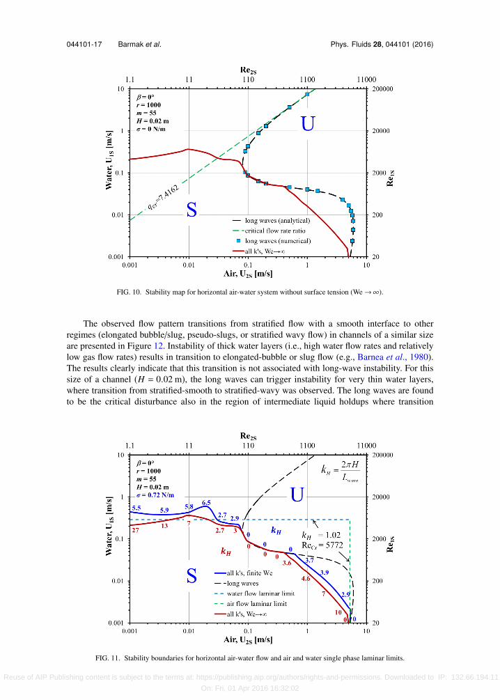
FIG. 10. Stability map for horizontal air-water system without surface tension (We → ∞).

The observed flow pattern transitions from stratified flow with a smooth interface to otherregimes (elongated bubble/slug, pseudo-slugs, or stratified wavy flow) in channels of a similar sizeare presented in Figure 12. Instability of thick water layers (i.e., high water flow rates and relativelylow gas flow rates) results in transition to elongated-bubble or slug flow (e.g., Barnea et al., 1980).The results clearly indicate that this transition is not associated with long-wave instability. For thissize of a channel (H = 0.02 m), the long waves can trigger instability for very thin water layers,where transition from stratified-smooth to stratified-wavy was observed. The long waves are foundto be the critical disturbance also in the region of intermediate liquid holdups where transition

FIG. 11. Stability boundaries for horizontal air-water flow and air and water single phase laminar limits.

Reuse of AIP Publishing content is subject to the terms at: https://publishing.aip.org/authors/rights-and-permissions. Downloaded to IP: 132.66.194.11

On: Fri, 01 Apr 2016 16:32:02

044101-18 Barmak et al. Phys. Fluids 28, 044101 (2016)

FIG. 12. Flow transition across stability boundary and sampling points for studying the critical perturbations in the horizontalair-water flow.

from stratified-smooth to pseudo-slugs was observed, implying that this transition is associated withlong-wave instability.

The loss of the flow stability may be initiated in the bulk of one or both phases (shear mode)and may thus be associated with laminar/turbulent transition in the corresponding phases, or at theinterface between the fluids (interfacial mode). When compared with the stability limits of air andwater single phase flow (corresponding to ReCr = 5772, critical wavenumber kH = 1.02, Figure 11),one can observe that the water flow is stabilized by the presence of a thin (less viscous and ligh-ter) gas layer at the upper wall. For the other extreme case of a thin water layer, the two-phasestability boundary almost coincides with the stability boundary of single phase air flow, implyingthat instability is driven by growing perturbations in the bulk of the air layer. However, due to thepresence of interface and surface tension, this process is characterized by longer wavelength criticaldisturbance.

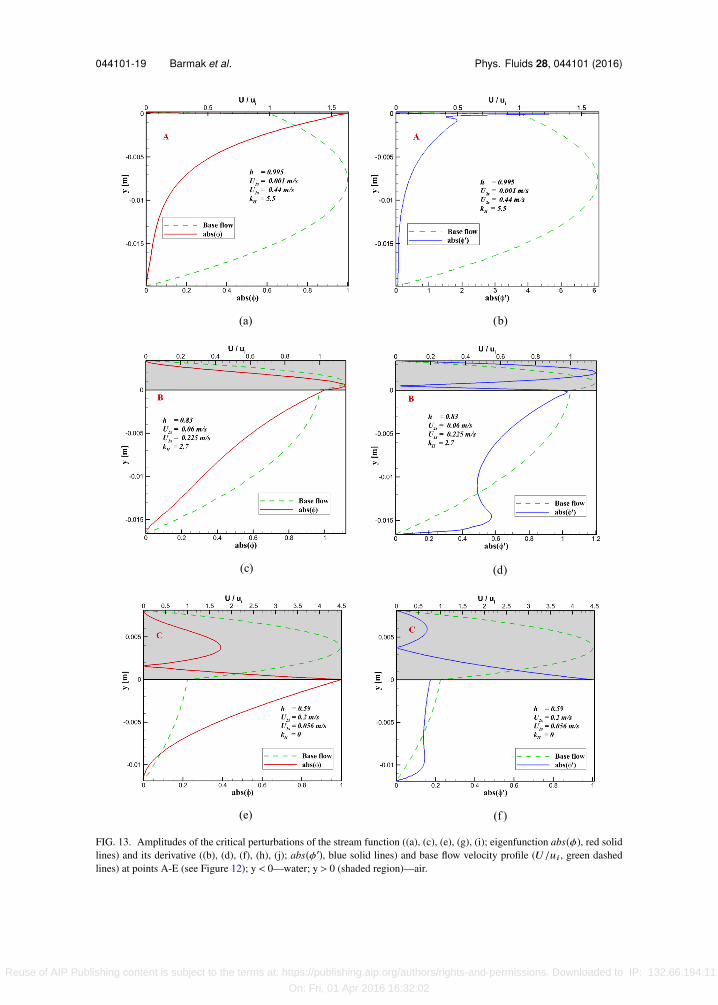
To study the locations at which instability evolves, the five points along the neutral stabilitycurve are taken (see Figure 12). The amplitudes of perturbations of the stream function and itsderivative for the point A (very thin layer of the air above the water) are shown in Figures 13(a)and 13(b). The maxima in the amplitude of both the vertical and horizontal velocity disturbances(perturbations of the stream function and its derivative, respectively) are at the interface, whereasin the original base flow the maximum velocity is located within the water layer. In this case thethin layer of air flow above the water has a stabilizing effect on the shear mode instability due tothe diminishing shear at the upper boundary. Upon increasing the water flow rate, instability is trig-gered at the water-air interface, suggesting that the flow is destabilized by a short wave interfacialmode.

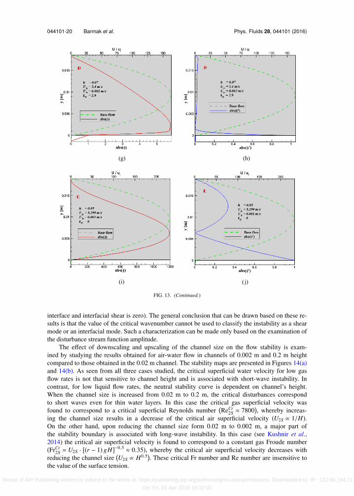
For higher flow rates of air (point B) the most unstable mode is a short wave with the maximumdisturbance amplitude in the air layer, close both to the interface and to the location of the maximalbase flow velocity (see Figures 13(c) and 13(d)). A further decrease in the holdup (increase in the airflow rate) brings us to the region where very long waves are the most unstable perturbations (pointC). The disturbance in this case can be characterized as interfacial mode, however another smallermaximum in the bulk of air is observed (see Figures 13(e) and 13(f)). In the region of small waterflow rates (point D, Figures 13(g) and 13(h)) the disturbance maximum within the air layer becomesdominant. This occurs since a sufficiently thin layer of the more viscous phase (water) plays a roleof wall for the air flow, and only a local (smaller) maximum is preserved at the interface. Themost unstable wavelength in this case is still small (kH = 2.9), but there is the second dangerouslong-wave mode, which subsequently becomes the most unstable for lower water holdups (point E,Figures 13(i) and 13(j)). Yet, in this case instability evolves in the bulk of the air layer, implyingshear mode instability, however, with a long wave. Inspection of Figure 13 indicates that due to thelarge viscosity ratio, the disturbance in the axial velocity attains a maximum value at the interface(except in the particular case where the maximum velocity of the primary flow is located at the

Reuse of AIP Publishing content is subject to the terms at: https://publishing.aip.org/authors/rights-and-permissions. Downloaded to IP: 132.66.194.11

On: Fri, 01 Apr 2016 16:32:02

044101-19 Barmak et al. Phys. Fluids 28, 044101 (2016)

FIG. 13. Amplitudes of the critical perturbations of the stream function ((a), (c), (e), (g), (i); eigenfunction abs(φ), red solidlines) and its derivative ((b), (d), (f), (h), (j); abs(φ′), blue solid lines) and base flow velocity profile (U/ui, green dashedlines) at points A-E (see Figure 12); y < 0—water; y > 0 (shaded region)—air.

Reuse of AIP Publishing content is subject to the terms at: https://publishing.aip.org/authors/rights-and-permissions. Downloaded to IP: 132.66.194.11

On: Fri, 01 Apr 2016 16:32:02

044101-20 Barmak et al. Phys. Fluids 28, 044101 (2016)

FIG. 13. (Continued.)

interface and interfacial shear is zero). The general conclusion that can be drawn based on these re-sults is that the value of the critical wavenumber cannot be used to classify the instability as a shearmode or an interfacial mode. Such a characterization can be made only based on the examination ofthe disturbance stream function amplitude.

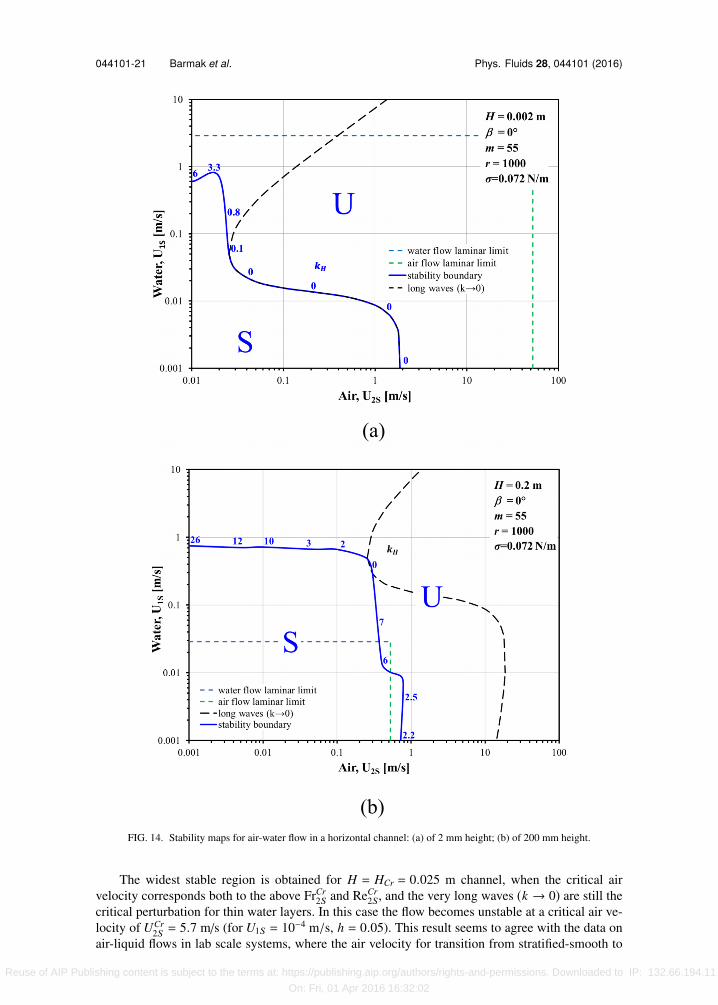
The effect of downscaling and upscaling of the channel size on the flow stability is exam-ined by studying the results obtained for air-water flow in channels of 0.002 m and 0.2 m heightcompared to those obtained in the 0.02 m channel. The stability maps are presented in Figures 14(a)and 14(b). As seen from all three cases studied, the critical superficial water velocity for low gasflow rates is not that sensitive to channel height and is associated with short-wave instability. Incontrast, for low liquid flow rates, the neutral stability curve is dependent on channel’s height.When the channel size is increased from 0.02 m to 0.2 m, the critical disturbances correspondto short waves even for thin water layers. In this case the critical gas superficial velocity wasfound to correspond to a critical superficial Reynolds number

�ReCr

2S ≈ 7800�, whereby increas-

ing the channel size results in a decrease of the critical air superficial velocity (U2S ∝ 1/H).On the other hand, upon reducing the channel size form 0.02 m to 0.002 m, a major part ofthe stability boundary is associated with long-wave instability. In this case (see Kushnir et al.,2014) the critical air superficial velocity is found to correspond to a constant gas Froude number(FrCr

2S = U2S · [(r − 1) gH]−0.5 ≈ 0.35), whereby the critical air superficial velocity decreases withreducing the channel size

�U2S ∝ H0.5�

. These critical Fr number and Re number are insensitive tothe value of the surface tension.

Reuse of AIP Publishing content is subject to the terms at: https://publishing.aip.org/authors/rights-and-permissions. Downloaded to IP: 132.66.194.11

On: Fri, 01 Apr 2016 16:32:02

044101-21 Barmak et al. Phys. Fluids 28, 044101 (2016)

FIG. 14. Stability maps for air-water flow in a horizontal channel: (a) of 2 mm height; (b) of 200 mm height.

The widest stable region is obtained for H = HCr = 0.025 m channel, when the critical airvelocity corresponds both to the above FrCr

2S and ReCr2S, and the very long waves (k → 0) are still the

critical perturbation for thin water layers. In this case the flow becomes unstable at a critical air ve-locity of UCr

2S = 5.7 m/s (for U1S = 10−4 m/s, h = 0.05). This result seems to agree with the data onair-liquid flows in lab scale systems, where the air velocity for transition from stratified-smooth to

Reuse of AIP Publishing content is subject to the terms at: https://publishing.aip.org/authors/rights-and-permissions. Downloaded to IP: 132.66.194.11

On: Fri, 01 Apr 2016 16:32:02

044101-22 Barmak et al. Phys. Fluids 28, 044101 (2016)

FIG. 15. Stable regions for (a) infinite long waves (k → 0) and (b) short waves (k = 10). Air-water flow without surfacetension under zero-gravity condition is unstable for all flow rates for very short waves (k → ∞), hence, for all wavenumberperturbations.

stratified-wavy was found to be about 5 m/s at atmospheric pressure (e.g., Andritsos and Hanratty,1987).

The above results can be presented in a form of general expressions for the critical channelheight and the corresponding maximum critical gas superficial velocity

HCr ≈

�ReCr

2S

�2µ2

2�FrCr

2S

�2ρ2

2g (r − 1)

1/3

, (26)

UCr2S =

ReCr2Sµ2

ρ2HCr= [(r − 1)gHCr]1/2 FrCr

2S. (27)

For channels larger than HCr, the effect of the channel size on the transitional U2S shouldbe evaluated based on

�ReCr

2S ≈ 7800�, whereas for H < HCr the scaling should be based on FrCr

2S.Moreover, the above scaling rules apply also for predicting the effect of pressure on the criticalgas velocity. Applying Eqs. (26) and (27) for high-pressure systems (r < 1000) indicates that foreach particular density ratio there is a critical channel height for which the stable stratified flowextends over a largest range of air flow rates. The scaling based on the Fr number (i.e., U2S ≈(ρ2o/ρ2)0.5(U2S)o suggested by (Andritsos and Hanratty, 1987), subscript o denotes atmosphericconditions) may be applicable only to channels of H < HCr. For H > HCr, the scaling based onRe suggests that U2S ∝ 1/ρ2. At elevated pressures, the critical channel size and the correspondingmaximal UCr

2S decrease according to Eqs. (26) and (27), implying that the range of gas flow ratesfor which stratified flow with a smooth interface can be maintained in field operations, which areassociated with large channel sizes and elevated pressures, is much smaller than that obtained in

FIG. 16. Stability map for air-water system with surface tension under zero-gravity condition.

Reuse of AIP Publishing content is subject to the terms at: https://publishing.aip.org/authors/rights-and-permissions. Downloaded to IP: 132.66.194.11

On: Fri, 01 Apr 2016 16:32:02

044101-23 Barmak et al. Phys. Fluids 28, 044101 (2016)

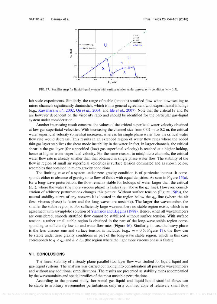
FIG. 17. Stability map for liquid-liquid system with surface tension under zero-gravity condition (m = 0.5).

lab scale experiments. Similarly, the range of stable (smooth) stratified flow when downscaling tomicro channels significantly diminishes, which is in a general agreement with experimental findings(e.g., Kawahara et al., 2002; Qu et al., 2004; and Ide et al., 2007). Note that the critical Fr and Reare however dependent on the viscosity ratio and should be identified for the particular gas-liquidsystem under consideration.

Another interesting result concerns the values of the critical superficial water velocity obtainedat low gas superficial velocities. With increasing the channel size from 0.02 m to 0.2 m, the criticalwater superficial velocity somewhat increases, whereas for single phase water flow the critical waterflow rate would decrease. This results in an extended region of water flow rates where the addedthin gas layer stabilizes the shear mode instability in the water. In fact, in larger channels, the criticalshear in the gas layer (for a specified (low) gas superficial velocity) is reached at a higher holdup,hence at higher water superficial velocity. For the same reason, in mini/micro channels, the criticalwater flow rate is already smaller than that obtained in single phase water flow. The stability of theflow in region of small air superficial velocities is surface tension dominated and as shown below,resembles that obtained in micro gravity conditions.

The limiting case of a system under zero gravity condition is of particular interest. It corre-sponds either to absence of gravity or to flow of fluids with equal densities. As seen in Figure 15(a),for a long-wave perturbation, the flow remains stable for holdups of water larger than the critical(hcr), where the water (the more viscous phase) is faster (i.e., above the qcr line). However, consid-eration of arbitrary perturbations changes this picture. Without surface tension (Figure 15(b)), theneutral stability curve of any nonzero k is located in the region below the qcr line (where the air(less viscous phase) is faster and the long waves are unstable). The larger the wavenumber, thesmaller the stable region is. For sufficiently large wavenumbers no stable region exists, which is inagreement with asymptotic solution of Yiantsios and Higgins (1988). Hence, when all wavenumbersare considered, smooth stratified flow cannot be stabilized without surface tension. With surfacetension, a rather small stable region is obtained in the part of the long-wave stable region corre-sponding to sufficiently low air and water flow rates (Figure 16). Similarly, in case the heavy phaseis the less viscous one and surface tension is included (e.g., m = 0.5, Figure 17), the flow canbe stable under zero gravity conditions in part of the long-wave stable region, which in this casecorresponds to q < qcr and h < hcr (the region where the light more viscous phase is faster).

VII. CONCLUSIONS

The linear stability of a steady plane-parallel two-layer flow was studied for liquid-liquid andgas-liquid systems. The analysis was carried out taking into consideration all possible wavenumbersand without any additional simplifications. The results are presented as stability maps accompaniedby the wavenumbers and spatial profiles of the most unstable perturbations.

According to the present study, horizontal gas-liquid and liquid-liquid stratified flows canbe stable to arbitrary wavenumber perturbations only in a confined zone of relatively small flow

Reuse of AIP Publishing content is subject to the terms at: https://publishing.aip.org/authors/rights-and-permissions. Downloaded to IP: 132.66.194.11

On: Fri, 01 Apr 2016 16:32:02

044101-24 Barmak et al. Phys. Fluids 28, 044101 (2016)

rates. This is in agreement with experimental observations, but not predicted by long-wave analysis(see Kushnir et al., 2014). Nevertheless, identification of systems and conditions where a long-wavedisturbance is the critical one for triggering instability is of importance, as under such conditions thelong-wave analytical solution (or the two-fluid model) can be conveniently applied for predictingthe stable stratified flow boundaries.

Short-wave instability is a characteristic of thin layers of the less viscous fluid, whereas inter-mediate and long-wave perturbations may be dominant in triggering instability of small holdupsof the more viscous fluid. Depending on the flow conditions, the critical perturbation can evolvemainly at the interface (so-called “interfacial mode instability”) or in the bulk of one of the phases(i.e., “shear mode”). However, it was shown that there is no definite correlation between the typeof instability and the perturbation wavelength. In particular, long waves do not necessarily implyinterfacial mode instability. A classification to shear or interfacial mode can be made only based onexamination of the pattern of the disturbance stream function.

Additionally, the effect of the channel height on the stability of gas-liquid flow was studied.It was revealed that in small channels and small holdups, a long wave is the critical disturbance.In this case the channel size effect on the critical gas superficial velocity for the onset of insta-bility is scaled by a critical gas (superficial) Froude number. On the other hand, in large channels,short/intermediate waves are the critical disturbances, and the channel size effect on the criticalgas velocity is scaled by a critical gas (superficial) Reynolds number. Long waves become thecritical perturbations in channel heights less than a critical one. The latter can be determined foreach particular density ratio (i.e., operational pressure). An increase of the channel height abovethe critical one results in a decrease of the critical gas flow rate, owing to short-wave instability. Inchannel of the critical height, a stable stratified flow region can be obtained for the largest rangeof gas flow rates corresponding to both the critical Froude and the critical Reynolds numbers.The values of the critical Fr and Re numbers are however dependent on the viscosity ratio. Thesefindings are of practical importance especially for upscaling lab-scale (and low pressure) data on thestratified-smooth boundary to field operational conditions.

The surface tension was shown to affect more the short-waves instability. However, due to theexistence of other growing modes with larger wavelength, the surface tension effect on the stabilityboundaries is found to be rather small. The only exceptions are system under zero-gravity conditionand flows in microchannels, where capillarity becomes significant. In the absence of a gravitationalforce, the surface tension plays a leading role in the flow stabilization, and for sufficiently small flowrates the flow is stable to all disturbances.

Andritsos, N. and Hanratty, T. J., “Interfacial instabilities for horizontal gas-liquid flows in pipelines,” Int. J. Multiphase Flow13, 583–603 (1987).

Andritsos, N., Williams, L., and Hanratty, T. J., “Effect of liquid viscosity on the stratified-slug transition in horizontal pipeflow,” Int. J. Multiphase Flow 15, 877–892 (1989).

Barnea, D., Shoham, O., Taitel, Y., and Dukler, A. E., “Flow pattern transition for gas-liquid flow in horizontal and inclinedpipes,” Int. J. Multiphase Flow 6, 217–225 (1980).

Barnea, D. and Taitel, Y., “Interfacial and structural stability of separated flow,” Int. J. Multiphase Flow 20, 387–414 (1994).Birvalski, M., Tummers, M. J., Delfos, R., and Henkes, R. A. W. M., “PIV measurements of waves and turbulence in stratified

horizontal two-phase pipe flow,” Int. J. Multiphase Flow 62, 161–173 (2014).Boomkamp, P. A. M. and Miesen, R. H. M., “Classification of instabilities in parallel two-phase flow,” Int. J. Multiphase Flow

22, 67–88 (1996).Brauner, N. and Moalem Maron, D., “Analysis of stratified/nonstratified transitional boundaries in horizontal gas-liquid flows,”

Chem. Eng. Sci. 46, 1849–1859 (1991).Brauner, N. and Moalem Maron, D., “The role of interfacial shear modelling in predicting the stability of stratified two-phase

flow,” Chem. Eng. Sci. 48, 2867–2879 (1993).Charles, M. E. and Lilleleht, L. U., “An experimental investigation of stability and interfacial waves in co-current flow of two

liquids,” J. Fluid Mech. 22, 217–224 (1965).Francis, J. G. F., “The QR transformation—Part 2,” Comput. J. 4, 332–345 (1962).Goldstein, A., Ullmann, A., and Brauner, N., “Characteristic of stratified laminar flows in inclined pipes,” Int. J. Multiphase

Flow 75, 267–287 (2015).Hesla, T. I., Pranckh, F. R., and Preziosi, L., “Squire’s theorem for two stratified fluids,” Phys. Fluids 29, 2808–2811 (1986).Hooper, A. P. and Boyd, W. S. G., “Shear-flow instability at the interface between two viscous fluids,” J. Fluid Mech. 128,

507–528 (1983).Ide, H., Kariyasaki, A., and Fukano, T., “Fundamental data on the gas-liquid two-phase flow in minichannels,” Int. J. Therm.

Sci. 46, 519–530 (2007).

Reuse of AIP Publishing content is subject to the terms at: https://publishing.aip.org/authors/rights-and-permissions. Downloaded to IP: 132.66.194.11

On: Fri, 01 Apr 2016 16:32:02

044101-25 Barmak et al. Phys. Fluids 28, 044101 (2016)

Kaffel, A. and Riaz, A., “Eigenspectra and mode coalescence of temporal instability in two-phase channel flow,” Phys. Fluids27, 042101 (2015).

Kawahara, A., Chung, P. M.-Y., and Kawaji, M., “Investigation of two-phase flow pattern, void fraction and pressure drop ina microchannel,” Int. J. Multiphase Flow 28, 1411–1435 (2002).

Kordyban, E. S. and Ranov, T., “Mechanism of slug formation in horizontal two-phase flow,” J. Basic Eng. 92, 857–864 (1970).Kushnir, R., Segal, V., Ullmann, A., and Brauner, N., in ICMF 2007: Proceedings of the 6th International Conference on

Multiphase Flow, Leipzig, Germany, July 9-13 2007, pp. S5_Tue_C_25 2007 (pp. 1-12), CD-ROM.Kushnir, R., Segal, V., Ullmann, A., and Brauner, N., “Inclined two-layered stratified channel flows: Long wave stability

analysis of multiple solution regions,” Int. J. Multiphase Flow 62, 17–29 (2014).Lin, P. Y. and Hanratty, T. J., “Prediction of the initiation of slugs with linear stability theory,” Int. J. Multiphase flow 12, 79–98

(1986).Mishima, K. and Ishii, M., “Theoretical prediction of onset of horizontal slug flow,” J. Fluids Eng. 102(4), 441–445 (1980).Orszag, S. A., “Accurate solution of the Orr-Sommerfeld stability equation,” J. Fluid Mech. 50, 689–703 (1971).Qu, W., Yoon, S.-M., and Mudawar, I., “Two-phase flow and heat transfer in rectangular micro-channels,” J. Electron. Packag.

126, 288–300 (2004).Segal, V., M.S. thesis, Tel Aviv University, 2008.Taitel, Y. and Dukler, A. E., “A model for predicting flow regime transitions in horizontal and near horizontal gas-liquid flow,”

AIChE J. 22, 47–55 (1976).Tilley, B. S., Davis, S. H., and Bankoff, S. G., “Linear stability of two-layer fluid flow in an inclined channel,” Phys. Fluids 6,

3906–3922 (1994).Tilley, B. S., Ph.D. thesis, Northwestern University, 1994.Tzotzi, C. and Andritsos, N., “Interfacial shear stress in wavy stratified gas-liquid flow in horizontal pipes,” Int. J. Multiphase

Flow 54, 43–54 (2013).Ullmann, A., Zamir, M., Ludmer, Z., and Brauner, N., “Stratified laminar countercurrent flow of two liquid phases in inclined

tubes,” Int. J. Multiphase Flow 29, 1583–1604 (2003).Ullmann, A., Goldstien, A., Zamir, M., and Brauner, N., “Closure relations for the shear stresses in two-fluid models for

stratified laminar flows,” Int. J. Multiphase Flow 30, 877–900 (2004).Vempati, B., Oztekin, A., and Neti, S., “Stability of two-layered fluid flows in an inclined channel,” Acta Mech. 209, 187–199

(2010).Wallis, G. B. and Dobson, J. E., “The onset of slugging in horizontal stratified air-water flow,” Int. J. Multiphase Flow 1,

173–193 (1973).Wu, H. L., Pots, B. F. M., Hollenberg, J. F., and Meerhoff, R., in Proceedings of the 3rd International conference on

Multiphase Flow, The Hague, Netherlands (BHRA, Cranfield, Bedford, England, 1987), pp. 13–21.Yiantsios, S. G. and Higgins, B. G., “Linear stability of plane Poiseuille flow of two superposed fluids,” Phys. Fluids 31,

3225–3238 (1988).Yih, C. S., “Instability due to viscosity stratification,” J. Fluid Mech. 27, 337–352 (1967).Yu, H. S. and Sparrow, E. M., “Experiments on two-component stratified flow in a horizontal duct,” J. Heat Transfer 91, 51–58

(1969).

Reuse of AIP Publishing content is subject to the terms at: https://publishing.aip.org/authors/rights-and-permissions. Downloaded to IP: 132.66.194.11

On: Fri, 01 Apr 2016 16:32:02