Stability of preferences and personality: Newevidence from developing and developed

countries.

Buly Cardak (La Trobe), Edwin Ip (Monash), NicolasSalamanca (Melbourne), Joe Vecci (Gothenburg)

Nordic Development Conference

June 11, 2018

Introduction

What do we mean by stability?

I Strict definition: Preferences are stable over time(Schildberg-Hrisch, 2018, JEP)

I Assume we are interested in risk preferencesI Implies that, in the absence of measurement error, one should

observe the same willingness to take risks when measuring anindividuals risk preferences repeatedly over time.

I Conditional or unconditional stability: control for observablecharacteristics i.e stability conditional on characteristics suchas income?

Introduction

A common assumption in economics (psychology, management andmarketing) is that preferences are static primitives fixed over time

I Convenient for modeling (tractability)I Critical for welfare analysis (ceteris paribus) and policy

I Convenient for empirical work (no simultaneity)

However, preferences could change...

I ... due to events in people’s lives

I ... naturally over time

I ... or because they are measured with error (i.e., they onlyseem to change)

Introduction

I Despite the importance of this topic it is difficult to estimatethe dynamic properties of preferences.

I Difficult with observational dataI Experimental data is limitedI Requires panel data with measured preferencesI Measurement error

Literature

Three main methods of analysing preference stability

1 Levels: preferencet = f (charasteristics)

e.g, Malmendier and Nagel 2011; Dohmen et al., 2011, 2012I Method better suited to analysing heterogenity of preferencesI Method is silent about stability

Literature

2 Changes: ∆preferencet = f (charasteristics)

e.g., Cobb-Clark and Schurer, 2012, 2013; Carlsson et al, 2014;Guiso et al., (forthcoming)

I Model examines the characteristics that impact change.I Not the same as stability especially in models with bad fit

(e.g., R2 <0.05)I Cannot differentiate unexplained variance in preference from

noiseI Does not formally test stability

Literature

3 Test-retest (psychology): preferencet = f (preferencet−k)

e.g., Fraley and Roberts, 2005; Meier and Sprenger, 2015;Chuang and Schechter, 2015

I Measures the amount preferences in the past explain currentpreferences.

I Current models do not clearly define a null hypothesis to testagainst

I Not able to separate changes due to measurement errorI Results could reflect both measurement error and predictable

changes due to background characteristicsI Mostly small non-representative datasets measuring short term

changes e.g, Meier and Sprenger, (2015) use data from2007-2008

Literature

Measurement Error

I Meier and Sprenger, 2015 find ”a high correlation at theindividual level, (but) there remains instability....largelyindependent of demographics and situational changes,potentially attributable to error”

I Similarly, Chuang and Schechter, 2015 argue that variability inpreferences maybe mostly due to noise- ‘data seems too noisyto estimate stability”

I Frederick, Loewenstein, and ODonoghue 2002 review the timepreference literature

I Discount rates ranging from 0 percent to thousands ofpercent per annum.

I They argue that differences may be due to measurement error.

What do we do?

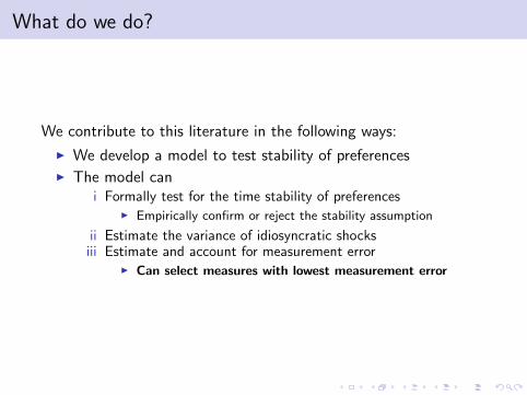
We contribute to this literature in the following ways:

I We develop a model to test stability of preferencesI The model can

i Formally test for the time stability of preferencesI Empirically confirm or reject the stability assumption

ii Estimate the variance of idiosyncratic shocksiii Estimate and account for measurement error

I Can select measures with lowest measurement error

What do we do?

I Using this model we test risk and time preferences, the BigFive personality traits, trust and locus of control

I In Australia, Germany, Netherlands, United States, Thailand,Vietnam and Kyrgyzstan

i Use nationally representative panel datasetsii Over 140,000 individualsiii Over 4-20 yearsiiii Most comprehensive analysis on the topic

What do we do?

I Important contribution is the analysis of both developed anddeveloping countries

I Stability could differ between these two groups for a number ofreasons- more shocks in developing countries

I Many program in developing countries attempt to changepreferences (either explicitly or implicitly)

I Its important to understand the malleability of preferences

Model

The Model

Model

Pit = P∗it + εit (1)

P∗it = αP∗

i ,t−1 + g(Xit) + ηit (2)

where

Pit ≡ person i ’s measured level of preference at time t

P∗it ≡ latent preferences

g(Xit) ≡ observable characteristics

ηit ≡ idiosyncratic shocks to preferences

εit ≡ measurement error

Eq 2 defines the evolution of latent preferences P∗it as an

AR(1) autoregressive process with a drift g(Xit)

Model

First, replace (2) into (1)

Pit = αPi ,t−1 + g(Xit) + {ηit + εit − αεi ,t−1} (3)

All elements are observable

1 The autoregressive parameter α shows the intra-individualstability of Pit i.e past to present

2 g(Xit) (drift) allows preferences to tend towards a conditionalmean level determined by observables

I Think of this as the level to which preferences tend to onceautocorrelation has been accounted.

Model

First, replace (2) into (1)

Pit = αPi ,t−1 + g(Xit) + {ηit + εit − αεi ,t−1} (3)

I Xit will capture factors that impact the conditional level towhich preferences tend

3 ηit are the idiosyncratic shocks i.e the importance ofconditional variation in latent preferences

4 εit will quantify the measurement error

Model

To find variance of idiosyncratic shocks (σ2η), and of measurementerror (σ2ε):

1 It is easier to work with P̃it , which is P∗it net of g(Xit)

2 With some algebra

Var(P̃i ,t+k−( α̂k)P̃it |X̃i , t+k) = σ2η

k∑j=0

α̂2j+σ2ε(α̂2k+1); k = 1, ...,K

(4)

I Working Click

3 Then solve a 2-unknown, K ≥ equation system

Estimation

Estimation in a two-step process:

1 GMM IV: Pit = αPi ,t−1 + g(Xit) + eitI OLS is biased since Pi,t−1 and εi,t−1 are correlatedI To obtain consistent estimates of the parameters we use the

moment conditions implied in a Generalised Method ofMoments (GMM) IV approach

I Pi,t−1 is instrumented by further lagsI Similar to a test retest correlation, but is not attenuated by

measurement error and nets out predictable variation due toobservable characteristics

I Standardise all measures

Estimation

I Test whether α = 1 i.e stability

Interpretation of α = 1I If compared to a test-retest correlation α = 1 would imply

perfect correlation over time and full stability.

Estimation

To estimate the variance of the errors:

2 Non-linear regression:

Var(P̃i ,t+k−( α̂k)P̃it |Xi , t+k) = e ln(σ2η)

k∑j=0

α̂2j+e ln(σ2ε)(α̂2k+1)+vk ;

(5)

k = 1, ...,K

with nonparametric bootstrap standard errors

Estimation

We also estimate a noise to signal ratio following Cameron andTrivedi, 2005, p903.

I A comparable metric of the amount of measurement error inpreferences across models

I Since Pit can be standardised to have unit variance we canestimate

s =σ2ε

(1− σ2ε)(6)

Data

1 Household, Income and Labour Dynamics in Australia(HILDA)

I Unbalanced yearly representative panel of Australianhouseholds

I Use data from 2001 to 2016. Approx 5,000 individuals perwave.

I RiskI Question on financial risk.

I Risk elicited 13 times

Data

2 Dutch National Bank Household SurveyI Unbalanced representative yearly panel of Dutch households

since 1993I Risk aversion index

I 6 items, 1994-2015, 2,894 individuals

Data

3 German Socio-Economic Panel studyI Unbalanced representative panel of German households since

1984I Use data from 2004-2015, approx 4,400 individuals per year.I Risk:

I Question “Are you generally a person who is fully prepared totake risks, or do you try to avoid taking risks?”

I Response on a scale 0 (unwilling)-10 (fully prepared)I Experimentally validated by Dohmen et al (2011)

I TrustI Q: ”One can trust other people”I 5 point scaleI Measured in 2003, 2008, 2013

Data

4 US: American Life PanelI Unbalanced representative panel of US households collected by

RANDI Use data from 2008-2011, 3 waves, approx 1,252 individuals

per yearI Risk:

I Same question as GSOEP

Data

5 Thailand Socio Economic PanelI Panel representative of rural Thailand, 4 waves (2008, 2010,

2013, 2016), 1738 individuals per wave.I Funded by the German government and run by Leibniz

University HannoverI Risk:

I Same question as GSOEP

6 Vietnamese Socio Economic PanelI Panel representative of rural Vietnam, 4 waves (2008, 2010,

2013, 2016), 1764 individuals per wave.I Risk:

I Same question as GSOEP

Data

7 Life in KyrgyzstanI Panel representative of Kyrgyzstan, 4 waves (2010-2013), 3000

households and 8000 individuals per wave.I Low income country (World Bank)I Collected by DIW Berlin and HumboldtI Risk and Trust:

I Same questions as GSOEP

Data: Summary

Risk Patience Trust Big 5 Locus of Control Alturism

Australia Y Y YNetherlands Y YGermany Y Y Y YUS YThailand YVietnam YKyrgyzstan Y Y

I Controls for all data include: gender, age, income, education,employment and marital status

Results

Risk

Risk: Developed Countries, GMM IV

AusRisk

(1) (2)

Lagged risk aversion (α) 0.963 0.949(0.007) (0.008)

H0 : α = 1 [0.000] [0.000]Corrected risk aversion (α) 0.963 0.949

(0.007) (0.008)H0 : α = 1 [0.000] [0.000]

Idiosyncratic var. (σ2η) 0.080 0.083

(0.000) (0.000)Measurement error var. 0.391 0.390(σ2ε) (0.000) (0.000)

Noise to signal ratio 0.643 0.640(0.000) (0.000)

Controls No YesHo: joint sig. controls [0.000]Obs. 67,378 67,378

Risk: Developed Countries, GMM IV

Aus Dutch German USRisk Risk Risk Risk

(1) (2) (3) (4) (5) (6) (7) (8 )

Lagged risk aversion 0.963 0.949 0.970 0.966 0.992 0.992 1.027 0.944(α) (0.007) (0.008) (0.011) (0.010) (0.007) (0.008) (0.058) (0.059)H0 : α = 1 [0.000] [0.000] [0.012] [0.018] [0.176] [0.217] [0.636] [0.346]Corrected risk aversion 0.963 0.949 0.970 0.966 0.992 0.992 1.027 0.944(α) (0.007) (0.008) (0.008) (0.011) (0.007) (0.008) (0.058) (0.059)H0 : α = 1 [0.000] [0.000] [0.012] [0.018] [0.176] [0.217] [0.636] [0.346]

Idiosyncratic var. (σ2η) 0.080 0.083 0.047 0.048 0.071 0.057 0.000 0.000

(0.000) (0.000) (0.012) (0.012) (0.000) (0.000) (0.000) (0.000)Measurement err. var. 0.391 0.390 0.296 0.296 0.378 0.378 0.476 0.480

(σ2ε) (0.000) (0.000) (0.012) (0.012) (0.000) (0.000) (0.025) (0.003)

Noise to signal ratio 0.643 0.640 0.418 0.418 0.607 0.607 0.909 0.923(0.000) (0.000) (0.023) (0.023) (0.000) (0.000) (0.091) (0.011)

Controls No Yes No Yes No Yes No YesHo: joint sig. controls [0.000] [0.433] [0.000] [0.433] [0.000]Obs. 67,378 67,378 10,404 10,404 44,386 44,386 1,252 1,252

OLS

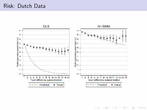
Risk: Dutch Data

Risk: Developing Countries, GMM IV

Thai Viet KyrgRisk Risk Risk

(1) (2) (3) (4) (5) (6)

Lagged risk aversion (α) 0.385 0.350 0.117 0.137 0.867 0.857(0.208) (0.234) (0.079) (0.128) (0.036) (0.044)

H0 : α = 1 [0.001] [0.003] [0.000] [0.000] [0.000] [0.001]Corrected risk aversion (α) 0.727 0.705 0.490 0.516 0.867 0.857

(0.131) (0.157) (0.079) (0.132) (0.036) (0.044)H0 : α = 1 [0.001] [0.003] [0.000] [0.000] [0.000] [0.001]

Idiosyncratic var. (σ2η) 1.215 2.289 55.523 48.628 0.511 0.578

(0.000) (0.000) (0.000) (0.000) (0.000) (0.000)

Measurement error var. (σ2ε) 0.785 0.684 0.224 0.005 0.328 0.287

(0.000) (0.000) (0.000) (0.000) (0.000) (0.000)Noise to signal ratio 3.645 2.164 0.289 0.005 0.487 0.402

(0.000) (0.000) (0.000) (0.000) (0.000) (0.000)

Controls No Yes No Yes No YesHo: joint sig. controls [0.002]

Obs. 1,738 1,738 1,764 1,764 6,781 6,781

Results

Trust

Trust

German KyrgTrust Trust

(1) (2) (3) (4)

Lagged trust (α) 0.909 0.906 1.154 1.149(0.045) (0.050) (0.093) (0.096)

H0 : α = 1 [0.000] [0.062] [0.097] [0.122]Corrected trust (α) 0.981 0.981 1.154 1.149

(0.010) (0.011) (0.093) (0.096)H0 : α = 1 [0.000] [0.062] [0.097] [0.122]

Idiosyncratic var. (σ2η) 0.196 0.173 0.255 0.291

(0.000) (0.000) (0.000) (0.000)Measurement error var. (σ2

ε) 0.512 0.511 0.591 0.565(0.000) (0.000) (0.000) (0.000)

Noise to signal ratio 1.049 1.044 1.448 1.300(0.000) (0.000) (0.000) (0.000)

Controls No Yes No YesHo: joint sig. controls [0.896]Obs. 4,662 4,662 6,430 6,430

Robustness

I Two important questions:

1 What if we assume stability when preferences are not stable?I For instance correlate risk at a point in time with outcomes

later

2 What is the severity of the bias when α! = 1

Robustness

To estimate severity of bias from extrapolation of preferencesI Simulate a contemporaneous relation between an outcomes yt

and preference Pt

I Simulate preferences using the data generating processevolving in equation 3 and 2

I Examine what happens when we increasingly use ‘stale”measures of preferences to predict outcomes yt

I As we increasingly use stale preferences (move further awayfrom the initial measure), estimates drift from the true effect.

I We can also simulate different rates of α in eq. 3 for eachmodel and then estimate the extent of the bias over years.

Stale Preferences

Simulation of OLS and IV-GMM estimates of a causal effectbetween an outcome and preferences with an increasingly stalepreference.

Conclusion

I We estimate a new model thatI Explicitly tests for stabilityI Addresses endogenityI Estimate the impact of changes in observable characteristics,

the variation due to idiosyncratic shocks and measurementerror

I We test stability of risk and time preferences, the Big Fivepersonality traits, altruism, trust and locus of control

I Across large, representative household panel datasets fromaround the world

I Generally find that preferences and traits have strongautoregressive components essentially rendering themtime-invariant

I This is not true for risk in developing countries.

Model

From equation 3, take the kth difference of P̃it and replacingrecursively yielding

P̃i ,t+k − P̃it = P̃∗i ,t+k + εi ,t+k − P̃∗

it − εit= αP̃∗

i ,t+k−1 + ηi ,t+k + εi ,t+k − P̃∗it − εit

...

= (αk − 1)P̃∗it +

k∑j=0

αjηi ,t+k−j+εi ,t+k − εit

Model

Replacing for P̃∗it and rearranging terms and simplifying, results in:

P̃i ,t+k − (αk)P̃it =k∑

j=0

αjηi ,t+k−j−αkεit + εi ,t+k (7)

= υi ,t+k

υi ,t+k represents the collection of all error and noise terms. TheLHS is expressed in terms of observable measures of P̃i ,t and the

parameter α which we have a consistent estimator

Model

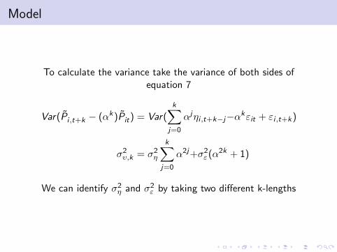
To calculate the variance take the variance of both sides ofequation 7

Var(P̃i ,t+k − (αk)P̃it) = Var(k∑

j=0

αjηi ,t+k−j−αkεit + εi ,t+k)

σ2υ,k = σ2η

k∑j=0

α2j+σ2ε(α2k + 1)

We can identify σ2η and σ2ε by taking two different k-lengths

Model

Working

Var(P̃i ,t+k−(αk)P̃it) = σ2η

k∑j=0

α2j +σ2ε(α2k +1); k = 1, ...,K (4)

For k = 1 and k = 2

σ2υ,1 = (α2 + 1)(σ2η + σ2ε)

σ2υ,2 =2∑

j=0

α2σ2η + (α4 + 1)σ2ε

I Back Click

OLS Risk: Developed Countries

Aus Dutch German USOLS OLS OLS OLSRisk Risk Risk Risk

(1) (2) (3) (4) (5) (6) (7) (8)

Lagged risk aversion (α) 0.571 0.530 0.653 0.641 0.585 0.561 0.498 0.441(0.005) (0.005) (0.017) (0.017) (0.005) (0.005) (0.026) (0.025)

H0 : α = 1 [0.000] [0.000] [0.000] [0.000] [0.000] [0.000]

Controls No Yes No Yes No Yes No YesHo: joint sig. controls [0.000] [0.000] [0.000] [0.000]

Obs. 67,378 67,378 10,404 10,404 44,386 44,386 1,252 1,252