Stability issues in multivalue numerical methods for ordinary differential equations · Stability...
12
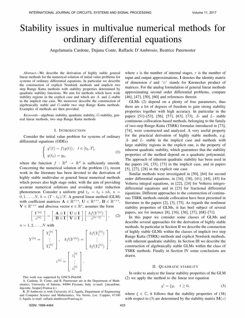
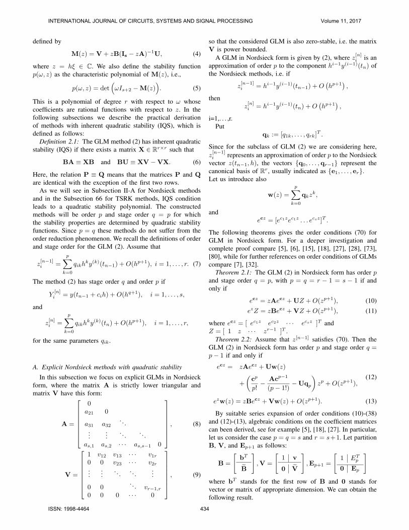
Stability issues in multivalue numerical methods for ordinary differential equations Angelamaria Cardone, Dajana Conte, Raffaele D’Ambrosio, Beatrice Paternoster Abstract—We describe the derivation of highly stable general linear methods for the numerical solution of initial value problems for systems of ordinary differential equations. In particular we describe the construction of explicit Nordsiek methods and implicit two step Runge Kutta methods with stability properties determined by quadratic stability functions. We aim for methods which have wide stability regions in the explicit case and which are A- and L-stable in the implicit one case. We moreover describe the construction of algebraically stable and G-stable two step Runge Kutta methods. Examples of methods are then provided. Keywords—algebraic stability, quadratic stability, G-stability, gen- eral linear methods, two step Runge Kutta methods I. I NTRODUCTION Consider the initial value problem for systems of ordinary differential equations (ODEs) { y ′ (t)= f (y(t)), t ∈ [t 0 ,T ], y(t 0 )= y 0 , (1) where the function f : R d → R d is sufficiently smooth. Concerning the numerical solution of the problem (1), recent work in the literature has been devoted to the derivation of highly stable multivalue or general linear numerical methods which posses also high stage order, with the aim of providing accurate numerical solutions and avoiding order reduction phenomenon. Consider a uniform grid t n = t 0 + nh, n = 0, 1,...,N , h =(T - t 0 )/N . A general linear method (GLM) with coefficient matrices A ∈ R s×s , U ∈ R s×r , B ∈ R r×s , V ∈ R r×r and abscissa vector c ∈ R s , assumes the form [ Y [n] z [n] ] = [ A ⊗ I U ⊗ I B ⊗ I V ⊗ I ][ hf (Y [n] ) z [n-1] ] , (2) n =1, 2,...,N with Y [n] = Y [n] 1 . . . Y [n] s , hf (Y [n] )= hf (Y [n] 1 ) . . . hf (Y [n] s ) , z [n] = z [n] 1 . . . z [n] r , This work was supported by GNCS-INdAM. A. Cardone, D. Conte, and B. Paternoster are in the Department of Math- ematics, University of Salerno, 84084 Fisciano, Italy. (e-mail: {ancardone, dajconte, beapat}@unisa.it.) R. D’Ambrosio is with University of L’Aquila, Department of Engineering and Computer Science and Mathematics, Via Vetoio, Loc. Coppito, 67100 L’Aquila (e-mail: [email protected]) where s is the number of internal stages, r is the number of input and output approximations, I denotes the identity matrix of dimension d and ‘⊗’ stands for Knonecker product of matrices. For the analog formulation of general linear methods approximating second order differential problems, compare [46], [47], [50], [60] and references therein. GLMs (2) depend on a plenty of free parameters, thus there are a lot of degrees of freedom to gain strong stability properties together with high accuracy. In particular in the papers [51]–[53], [56], [57], [63], [73], A- and L- stable continuous collocation-based methods, belonging to the family of two-step Runge-Kutta (TSRK) formulas introduced in [73], [74], were constructed and analyzed. A very useful property for the practical derivation of highly stable methods, e.g. A- and L- stable in the implicit case and methods with large stability regions in the explicit one, is the property of inherent quadratic stability, which guarantees that the stability properties of the method depend on a quadratic polynomial. The approach of inherent quadratic stability has been used in the papers [4], [35], [73] in the implicit case, and in papers [5], [27], [28] in the explicit one case. Similar methods were investigated in [50], [64] for second order differential equations, in [34], [38], [41], [44], [45] for Volterra integral equations, in [22], [24] for Volterra integro- differential equations and in [23] for fractional differential equations. Different approaches to the construction of continu- ous TSRK methods outside collocation have been presented in literature in the papers [2], [3], [75]. As regards the nonlinear stability properties of GLMs, it has beel subject of several papers, see for instance [8], [16], [36], [37], [68]–[71]. In this paper we consider some classes of GLMs and describe several approaches for the derivation of highly stable methods. In particular in Section II we describe the constuction of highly stable GLMs within the classes of implicit two step Runge Kutta (TSRK) methods and explicit Nordsiek methods, with inherent quadratic stability. In Section III we describe the construction of algebraically stable GLMs within the class of TSRK methods. Finally in Section IV some conclusions are drawn. II. QUADRATIC STABILITY In order to analyze the linear stability properties of the GLM (2) we apply the method to the linear test equation y ′ = ξy, t ≥ 0, (3) where ξ ∈ C, it follows that the stability properties of (38) with respect to (3) are determined by the stability matrix M(z) INTERNATIONAL JOURNAL OF CIRCUITS, SYSTEMS AND SIGNAL PROCESSING Volume 11, 2017 ISSN: 1998-4464 433
Transcript of Stability issues in multivalue numerical methods for ordinary differential equations · Stability...
Stability issues in multivalue numerical methods forordinary differential equations
Angelamaria Cardone, Dajana Conte, Raffaele D’Ambrosio, Beatrice Paternoster
Abstract—We describe the derivation of highly stable generallinear methods for the numerical solution of initial value problems forsystems of ordinary differential equations. In particular we describethe construction of explicit Nordsiek methods and implicit twostep Runge Kutta methods with stability properties determined byquadratic stability functions. We aim for methods which have widestability regions in the explicit case and which are A- and L-stablein the implicit one case. We moreover describe the construction ofalgebraically stable and G-stable two step Runge Kutta methods.Examples of methods are then provided.
Keywords—algebraic stability, quadratic stability, G-stability, gen-eral linear methods, two step Runge Kutta methods
I. INTRODUCTION
Consider the initial value problem for systems of ordinarydifferential equations (ODEs){
y′(t) = f(y(t)), t ∈ [t0, T ],
y(t0) = y0,(1)
where the function f : Rd → Rd is sufficiently smooth.Concerning the numerical solution of the problem (1), recentwork in the literature has been devoted to the derivation ofhighly stable multivalue or general linear numerical methodswhich posses also high stage order, with the aim of providingaccurate numerical solutions and avoiding order reductionphenomenon. Consider a uniform grid tn = t0 + nh, n =0, 1, . . . , N , h = (T −t0)/N . A general linear method (GLM)with coefficient matrices A ∈ Rs×s, U ∈ Rs×r, B ∈ Rr×s,V ∈ Rr×r and abscissa vector c ∈ Rs, assumes the form[
Y [n]
z[n]
]=
[A⊗ I U⊗ IB⊗ I V ⊗ I
] [hf(Y [n])
z[n−1]
], (2)
n = 1, 2, . . . , N with
Y [n] =
Y
[n]1...
Y[n]s
, hf(Y [n]) =
hf(Y
[n]1 )
...hf(Y
[n]s )
,
z[n] =
z[n]1...z[n]r
,This work was supported by GNCS-INdAM.A. Cardone, D. Conte, and B. Paternoster are in the Department of Math-
ematics, University of Salerno, 84084 Fisciano, Italy. (e-mail: {ancardone,dajconte, beapat}@unisa.it.)
R. D’Ambrosio is with University of L’Aquila, Department of Engineeringand Computer Science and Mathematics, Via Vetoio, Loc. Coppito, 67100L’Aquila (e-mail: [email protected])
where s is the number of internal stages, r is the number ofinput and output approximations, I denotes the identity matrixof dimension d and ‘⊗’ stands for Knonecker product ofmatrices. For the analog formulation of general linear methodsapproximating second order differential problems, compare[46], [47], [50], [60] and references therein.
GLMs (2) depend on a plenty of free parameters, thusthere are a lot of degrees of freedom to gain strong stabilityproperties together with high accuracy. In particular in thepapers [51]–[53], [56], [57], [63], [73], A- and L- stablecontinuous collocation-based methods, belonging to the familyof two-step Runge-Kutta (TSRK) formulas introduced in [73],[74], were constructed and analyzed. A very useful propertyfor the practical derivation of highly stable methods, e.g.A- and L- stable in the implicit case and methods withlarge stability regions in the explicit one, is the property ofinherent quadratic stability, which guarantees that the stabilityproperties of the method depend on a quadratic polynomial.The approach of inherent quadratic stability has been used inthe papers [4], [35], [73] in the implicit case, and in papers[5], [27], [28] in the explicit one case.
Similar methods were investigated in [50], [64] for secondorder differential equations, in [34], [38], [41], [44], [45] forVolterra integral equations, in [22], [24] for Volterra integro-differential equations and in [23] for fractional differentialequations. Different approaches to the construction of continu-ous TSRK methods outside collocation have been presented inliterature in the papers [2], [3], [75]. As regards the nonlinearstability properties of GLMs, it has beel subject of severalpapers, see for instance [8], [16], [36], [37], [68]–[71].
In this paper we consider some classes of GLMs anddescribe several approaches for the derivation of highly stablemethods. In particular in Section II we describe the constuctionof highly stable GLMs within the classes of implicit two stepRunge Kutta (TSRK) methods and explicit Nordsiek methods,with inherent quadratic stability. In Section III we describe theconstruction of algebraically stable GLMs within the class ofTSRK methods. Finally in Section IV some conclusions aredrawn.
II. QUADRATIC STABILITY
In order to analyze the linear stability properties of the GLM(2) we apply the method to the linear test equation
y′ = ξy, t ≥ 0, (3)
where ξ ∈ C, it follows that the stability properties of (38)with respect to (3) are determined by the stability matrix M(z)
INTERNATIONAL JOURNAL OF CIRCUITS, SYSTEMS AND SIGNAL PROCESSING Volume 11, 2017
ISSN: 1998-4464 433
defined by
M(z) = V + zB(Is − zA)−1U, (4)
where z = hξ ∈ C. We also define the stability functionp(ω, z) as the characteristic polynomial of M(z), i.e.,
p(ω, z) = det(ωIs+2 −M(z)
). (5)
This is a polynomial of degree r with respect to ω whosecoefficients are rational functions with respect to z. In thefollowing subsections we describe the practical derivationof methods with inherent quadratic stability (IQS), which isdefined as follows:
Definition 2.1: The GLM method (2) has inherent quadraticstability (IQS) if there exists a matrix X ∈ Rr×r such that
BA ≡ XB and BU ≡ XV −VX. (6)
Here, the relation P ≡ Q means that the matrices P and Qare identical with the exception of the first two rows.
As we will see in Subsection II-A for Nordsieck methodsand in the Subsection 66 for TSRK methods, IQS conditionleads to a quadratic stability polynomial. The constructedmethods will be order p and stage order q = p for whichthe stability properties are determined by quadratic stabilityfunctions. Since p = q these methods do not suffer from theorder reduction phenomenon. We recall the definitions of orderand stage order for the GLM (2). Assume that
z[n−1]i =
p∑k=0
qikhky(k)(tn−1) +O(hp+1), i = 1, . . . , r. (7)
The method (2) has stage order q and order p if
Y[n]i = y(tn−1 + cih) +O(hq+1), i = 1, . . . , s,
and
z[n]i =
p∑k=0
qikhky(k)(tn) +O(hp+1), i = 1, . . . , r,
for the same parameters qik.
A. Explicit Nordsieck methods with quadratic stability
In this subsection we focus on explicit GLMs in Nordsieckform, where the matrix A is strictly lower triangular andmatrix V have this form:
A =
0a21 0
a31 a32. . .
......
. . . . . .as,1 as,2 · · · as,s−1 0
, (8)
V =
1 v12 v13 · · · v1r0 0 v23 · · · v2r...
.... . . . . .
...
0 0. . . vr−1,r
0 0 0 · · · 0
, (9)
so that the considered GLM is also zero-stable, i.e. the matrixV is power bounded.
A GLM in Nordsieck form is given by (2), where z[n]i is anapproximation of order p to the component hi−1y(i−1)(tn) ofthe Nordsieck methods, i.e. if
z[n−1]i = hi−1y(i−1)(tn−1) +O
(hp+1
),
thenz[n]i = hi−1y(i−1)(tn) +O
(hp+1
),
i=1,. . . ,r.Put
qk := [q1k, . . . , qrk]T .
Since for the subclass of GLM (2) we are considering here,z[n−1]i represents an approximation of order p to the Nordsieck
vector z(tn−1, h), the vectors {q0, . . . ,qr−1} represent thecanonical basis of Rr, usually indicated as {e1, . . . , er}.Let us introduce also
w(z) =
p∑k=0
qkzk,
andecz = [ec1zec1z . . . ecsz]T .
The following theorems gives the order conditions (70) forGLM in Nordsieck form. For a deeper investigation andcomplete proof compare [5], [6], [15], [18], [27], [28], [73],[80], while for further references on order conditions of GLMscompare [7], [32].
Theorem 2.1: The GLM (2) in Nordsieck form has order pand stage order q = p, with p = q = r − 1 = s − 1 if andonly if
ecz = zAecz +UZ +O(zp+1), (10)
ezZ = zBecz +VZ +O(zp+1), (11)
where ecz = [ ec1z ec2z · · · ecsz ]T andZ = [ 1 z · · · zr−1 ]T .
Theorem 2.2: Assume that z[n−1] satisfies (70). Then theGLM (2) in Nordsieck form has order p and stage order q =p− 1 if and only if
ecz = zAecz +Uw(z)
+
(cp
p!− Acp−1
(p− 1!)−Uqp
)zp +O(zp+1),
(12)
ezw(z) = zBecz +Vw(z) +O(zp+1). (13)
By suitable series expansion of order conditions (10)-(38)and (12)-(13), algebraic conditions on the coefficient matricescan been derived, see for example [5], [18], [27]. In particular,let us consider the case p = q = s and r = s+1. Let partitionB, V, and Ep+1 as follows:
B =
[bT
B
],V =
[1 v
0 V
],Ep+1 =
[1 ET
p
0 Ep
]where bT stands for the first row of B and 0 stands forvector or matrix of appropriate dimension. We can obtain thefollowing result.
INTERNATIONAL JOURNAL OF CIRCUITS, SYSTEMS AND SIGNAL PROCESSING Volume 11, 2017
ISSN: 1998-4464 434

Theorem 2.3: [4] Assume that ci = cj , for any i = j andthat the GLM (2) with r = s + 1 has order and stage orderp = q = s. Then we have this representation of the matricesU and B:
U = Cp+1 −ACp+1Kp+1, (14)
bT = (ETp − v)C−1
p , (15)
andB = (Ep − V)C−1
p . (16)
In the case p = r = s = q + 1 a similar result can be proved,compare [5].
In order to simplify the search for methods with goodstability properties, we require that the method possesses thequadratic stability property, i.e. the stability function definedby (5) assumes this expression:
p(w, z) = wr−2(w2 − pr−1(z)w + pr−2(z)
), (17)
where
pr−1(z) = 1 + pr−1,1z + pr−1,2z2 + · · ·+ pr−1,sz
s,
pr−2(z) = pr−2,1z + pr−2,2z2 + · · ·+ pr−2,sz
s.(18)
A sufficient condition for the quadratic stability is IQS con-dition of Definition 2.1. In [4], [27] the following theoremwas proved, asserting that IQS condition leads to quadraticstability.
Theorem 2.4: Assume that the GLM (2) with matrices Aand V as in (8)-(9) has IQS. Then the stability function ofthe method assumes the form (17) with pr−1(z) and pr−2(z)given by (39).The structure of matrix X appearing in (6) is analyzed in thefollowing theorems [5], [27].
Theorem 2.5: For a GLM (2) with p = r = s and q = s−1,the most general matrix X satisfying conditions (6) is of theform:
X =
x1,1 x1,2 x1,3 . . . x1,s−1 x1,sx2,1 x2,2 x2,3 . . . x1,s−1 x2,s0 1 0 · · · 0 q3s0 0 1 · · · 0 q4s...
......
. . ....
0 0 0 · · · 1 qss
,
Theorem 2.6: For a GLM of type (2) with p = q = s andr = s+1, the most general matrix X satisfying conditions (6)is of the form:
X =
x1,1 x1,2 x1,3 · · · x1,r−1 x1,rx2,1 x2,2 x2,3 · · · x2,r−1 x2,r0 1 0 · · · 0 x3,r0 0 1 · · · 0 x4,r...
......
. . ....
...0 0 0 · · · 1 xr,r
,
In a symbolic computational environment, as Mathemati-car, we may find a family of GLMs of given order and IQS,depending on a set of free parameters. Then we may perform anumerical search for the method with maximal stability region.This is what it has been done in [5], [27], by suitably applying
−6 −5 −4 −3 −2 −1 0 10
0.5
1
1.5
2
2.5
3
3.5
Re(z)
Im(z
)
RKIQS
Fig. 1. Stability regions of RK method of order p = 4 and GLMs withp = q = s = 4, r = 5 with IQS
MATLAB functions like fminsearch. To obtain methods withlarger stability regions, the IQS requirement can be relaxed, byasking for quadratic stability (QS), i.e. the stability polynomialhas the form (17) [27], [28]. When the number of freeparameters is large, as it happens for high order methods, thenumerical search requires advanced optimization techniques,like those applied in [28].Now we provide an example of method with IQS and maximalstability region. We set p = q = s = 4, r = 5. We fix vectorc in advance. GLM method with the largest stability area hasarea equal to 18.3603, and error constant equal to -0.011. Thestability polynomial is
p(w, z) = w3(w2 − p4(z)w + p3(z)),
with
p4(z) = 1 + 293338z +
7871404z
2 + 18019828z
3 + 26598112560184z
4
p3(z) = − 45338z −
132518252z
2 + 1349127764z
3 + 681937163282392z
4.
The method coefficients are
c = [0,1
3,2
3, 1]T , (19)
A =
0 0 0 013 0 0 013
13 0 0
13
13
13 0
, (20)
V =
1 107
16920117 − 1
63 − 271
0 0 12
427 − 7
162
0 0 0 13
5108
0 0 0 0 16
0 0 0 0 0
. (21)
The other coefficient matrices can be derived from (14)-(16).In Fig. 1 we have plotted the stability region of this methodand, for comparison, the stability region of explicit Runge–Kutta methods of order 4.
An efficient and accurate variable-step algorithm for solvingnon-stiff ODEs, based on explicit GLMs of Nordsieck typewith QS or IQS must take into account fundamental issues,such as rescale strategy, local error estimation, step-changingstrategy and starting procedure. Here we illustrate the tech-nique that can be adopted. More details may be found in [6].First we set
z[n] =
[ynz[n]
],
INTERNATIONAL JOURNAL OF CIRCUITS, SYSTEMS AND SIGNAL PROCESSING Volume 11, 2017
ISSN: 1998-4464 435

where yn ≈ y(tn) and z[n] ≈ z(tn, hn), hn = tn− tn−1, with
z(t, h) :=
hy′(t)h2y′′(t)
...hpy(p)(t)
. (22)
Then GLM (2), on the nonuniform grid t0 < t1 < · · · <tN , tN ≥ T , can be formulated as (compare [73])
Y [n] = (e⊗ I)yn−1 + hn(A⊗ I)F (Y [n])
+ (U ⊗ I)z[n−1],
yn = yn−1 + hn(bT ⊗ I)F (Y [n]) + (vT ⊗ I)z[n−1],
z[n] = hn(B ⊗ I)F (Y [n]) + (V ⊗ I)z[n−1],(23)
where [A UB V
]=
A e U
bT 1 vT
B 0 V
, (24)
e = [1, . . . , 1]T ∈ Rs, b ∈ Rs, v ∈ Rr−1, A ∈ Rs×s, U ∈Rs×(r−1), B ∈ R(r−1)×s, V ∈ R(r−1)×(r−1).
The local error is analyzed by the following theorem [6](compare also [15], [20], [73])
Theorem 2.7: Assume that the input quantities to the cur-rent step from tn−1 to tn = tn−1 + hn satisfy
yn−1 = y(tn−1)
z[n−1] = z(tn−1, hn)− (β ⊗ I)hp+1n y(p+1)(tn−1)
+O(hp+2n )
(25)
where y(t) is the solution to the differential system (1) andrequire that
yn = y(tn)− Ehp+1n y(p+1)(tn) +O(hp+2
n )
z[n] = z(tn, hn)− (β ⊗ I)hp+1n y(p+1)(tn)
+O(hp+2n )
(26)
with the same vector β. Here, z(tn, hn) is the Nordsieck vectorcorresponding to the solution y(t) of the initial value problem{
y′(t) = f(y(t)), t ∈ [tn, tn+1],
y(tn) = yn.(27)
Then it follows that (26) holds if
E = 1(p+1)! −
bT cp
p! + vTβ,
β = (I − V )−1(tp −B cp
p!
),
tp =[
1p!
1(p−1)! . . . 1
]T.
(28)
According to the previous theorem, the local error is
le(tn) = Ehp+1n y(p+1)(tn) +O(hp+2
n ). (29)
The following result gives an estimate of the principal part ofthe local error, in the form
hp+1n y(p+1)(tn) = (φT ⊗ I)hnF (Y
[n])
+ (ψT ⊗ I)z[n−1] +O(hp+2n ), (30)
where I stands for the identity matrix of dimension d.Theorem 2.8: Consider the GLM (23) of order p and stage
order q = p and assume that f is sufficiently smooth. Thevectors φ ∈ Rs and ψ ∈ Rr−1 in (60) satisfy the linear system
φT cj−1
(j − 1)!+ ψj = 0, j = 1, 2, . . . , r − 1,
φT cp
p!− ψTβ = 1.
(31)
Now we apply the previous theorem to the case p = q = s =r − 1 = 4, which covers the example of method (19)-(21). Insuch case, linear system (31) gives
β =[
124
19
29108
12
]T, E =
26105531
1632823920(32)
φ =[−429 486 −243 54
]T, (33)
ψ =[132 −54 0 0
]T. (34)
In a variable-step algorithm, a rescale strategy is alsonecessary when we have computed z[n] ≈ z(tn, hn) andshould perform next step, since we need as a new input vectorz[n] ≈ z(tn, hn+1), with hn+1 = tn+1 − tn. A quite simplestrategy to compute z[n] consists of rescaling the vector z[n],i.e.:
z[n] = D(δ)z[n]
with D(δ) = diag(δ, δ2, . . . , δs), and δ = hn+1/hn.To complete the algorithm other ingredients are necessary, likean accurate starting procedure, a suitable choice of the initialstep-size and step control strategy. Many different techniquescan be applied, as illustrated in [6], [66], [67], [73].
For numerical comparison with other existing methods, weconsider the linear test problem
y′ = −λy, t ∈ [0, 10], (35)
for λ = 50 and the Prothero-Robinson type problem [78]{y′ = −16y + 15e−t, t ∈ [0, 100]y(0) = 2
(36)
with exact solution y(t) = e−t + e−16t.In Table I we list the error of Nordsieck method with IQSof order p = 4 (19)-(21) and of method with IRKS of thesame order, corresponding to η = 3/5 with error constantE = 1/300, whose coefficients are given in [19]. We observethat the IQS method converges for a larger value of stepsizewith respect to IRKS methods.
B. Implicit TSRK methods methods with quadratic stability
TSRK methods have the form
Y[n]i = uiyn−2 + (1− ui)yn−1
+ hs∑
j=1
(aijf(Y
[n−1]j ) + bijf(Y
[n]j )
),
yn = θyn−2 + (1− θ)yn−1
+ h
s∑j=1
(vjf(Y
[n−1]j ) + wjf(Y
[n]j )
),
(37)
INTERNATIONAL JOURNAL OF CIRCUITS, SYSTEMS AND SIGNAL PROCESSING Volume 11, 2017
ISSN: 1998-4464 436

TABLE IERRORS OF NORDSIECK METHOD AND IRKS METHOD OF ORDER p = 4
FOR PROBLEM (35), AND PROBLEM (36), WITH CONSTANT STEPSIZE.
problem (35), λ = 50
N h IQS p = 4 IRKS p = 471 0.14 8.33 · 10+74 1.75 · 10+97
81 0.13 5.59 · 10+54 4.42 · 10+82
91 0.11 3.70 · 10+26 1.28 · 10+60
101 0.10 2.92 · 10−04 3.48 · 10+30
111 0.09 2.83 · 10−18 2.97 · 10−09
problem (36)
N h IQS p = 4 IRKS p = 4311 0.32 1.02 · 10+11 1.06 · 10+128
321 0.31 3.68 · 10−16 2.85 · 10+95
331 0.30 1.02 · 10−35 8.50 · 10+59
341 0.29 1.08 · 10−45 1.08 · 10+21
351 0.28 4.14 · 10−46 1.47 · 10−22
i = 1, 2, . . . , s, n = 2, 3, . . . , N , Nh = T − t0. Here, yn isan approximation of order p to y(tn), tn = t0 +nh, and Y [n]
i
are approximations of stage order q to y(tn−1 + cih), i =1, 2, . . . , s, where y(t) is the solution to (1), c = [c1, . . . , cs]
T
is the abscissa vector and −1 < θ ≤ 1 for zero-stability.Methods (37) can be reformulated as GLMs of the formY [n]
yn
yn−1
hf(Y [n])
=
B e− u u A
wT 1− θ θ vT
0 1 0 0
Is 0 0 0
hf(Y [n])
yn−1
yn−2
hf(Y [n−1])
.(38)
This representation corresponds to the problem (1) with d = 1which is relevant in linear stability analysis. The matrices ofthe GLM (2) are then
[A U
B V
]=
B e− u u A
wT 1− θ θ vT
0 1 0 0Is 0 0 0
∈ R(2s+2)×(2s+2),
(39)In [35] the following theorem was proved, asserting that
IQS condition leads to quadratic stability.Theorem 2.9: Assume that the TSRK method (37) has IQS
and that the matrices Is− zA and Is+2− zX are nonsingular.Then its stability function p(ω, z) defined by (5) assumes theform
p(ω, z) = ωs(ω2 − p1(z)ω + p0(z)
), (40)
where p1(z) and p0(z) are rational functions with respect toz.
In this section we will consider implicit methods where thematrix A = B has a one point spectrum, i.e.
σ(B) = {λ}, λ > 0. (41)
The feature of being one point spectrum would allow for effi-cient implementation of such methods similarly as in the caseof singly implicit Runge-Kutta (SIRK) methods considered byBurrage [9], Butcher [12], and Burrage, Butcher and Chipman[10], see also [13], [15]. For methods for which the coefficient
matrix B has a one point spectrum (41) it is more convenientto work with the function p(ω, z) defined by
p(ω, z) = (1− λz)sp(ω, z), (42)
in which the coefficients of ωi, i = 0, 1, . . . , s + 2, arepolynomials of degree s with respect to z. Then the if theIQS condition is verified the polynomial assumes the simpleform
p(ω, z) = ωs((1− λz)sω2 − p1(z)ω + p0(z)
), (43)
with a root ω = 0 of multiplicity s, where p1(z) and p0(z)are polynomials of degree s with respect to z.
To express the IQS conditions (6) in terms of the coefficientsθ, u, v, w, A, and B of TSRK method (37) we partition thematrix X as follows
X =
[X11 X12
X21 X22
], (44)
where X11 ∈ R2×2, X12 ∈ R2×s, X21 ∈ Rs×2, X22 ∈ Rs×s.We also partition accordingly the matrices B, U, and V (see(39))
B =
[B11
Is
], U =
[U11 A
], V =
[V11 V120 0
],
where B11 ∈ R2×s, U11 ∈ Rs×2, V11 ∈ R2×2, V12 ∈ R2×s
are given by
B11 =
[wT
0
], U11 =
[e− u u
],
V11 =
[1− θ θ1 0
], V12 =
[vT
0
],
and 0 in V stands for zero matrices of dimension s × 2 ands× s, respectively.
Theorem 2.10: A TSRK method (37) has IQS if there existvectors α, β ∈ Rs and a matrix X ∈ Rs×s such that thefollowing conditions are statisfied
B = αwT +X, e = α+ β, u = θα, A = αvT . (45)
With the aim of constructing TSRK methods with IQShaving order p and stage order q = p, we recall (see [35])that, introducing the notation
C =
[c
c2
2!· · · cs
s!
], C =
[e
c
1!· · · cs−1
(s− 1)!
],
d =
[−1
1
2!· · · (−1)s
s!
]T, g =
[1
1
2!· · · 1
s!
]T,
E =
[e
c− e
1!· · · (c− e)s−1
(s− 1)!
],
then the order p and stage order q conditions, with q = p, forTSRK method (37) take the form
AE = C − udT −BC, vTE = gT − θdT − wT C. (46)
Moreover the polynomials p1(z) and p2(z) appearing in(43) take the form
p1(z) = 1− θ + p11z + · · ·+ p1szs,
INTERNATIONAL JOURNAL OF CIRCUITS, SYSTEMS AND SIGNAL PROCESSING Volume 11, 2017
ISSN: 1998-4464 437

p0(z) = −θ + p01z + · · ·+ p0szs.
Then the construction of highly stable TSRK methods (37)with IQS properties and coefficient matrix B with one pointspectrum σ(B) = {λ} can be summarized in the followingalgorithm.
1) Choose the abscissa vector c with distinct components,such that the matrices C and E defined at the beginningof this section are nonsingular.
2) As for methods of order p = s the stability polynomialp(ω, z) satisfies the condition
p(ez, z) = O(zs+1), z → 0, (47)
we solve this system by fixing s coefficients of thepolynomials p0(z) and p1(z) and deriving the remainings as functions of θ and λ. Choose the parameters θ andλ > 0 so that the stability polynomial p(ω, z) is A-stableand also L-stable, by using the Schur criterion.
3) Compute the coefficient matrix B from the formula
B = (C − αgT )C−1 + αwT ,
which is a consequence of (46) and the last condition in(45). This matrix depends on the vectors α and w.
4) Compute the vectors β and u from the second and thirdcondition of (45), i.e., β = e− α and u = θα.
5) Compute the coefficient matrix A and the vector v from(46) as
A = (C − udT −BC)E−1, (48)
andvT = (gT − θdT − wT C)E−1. (49)
They depend on α and w.6) In order to impose that σ(B) = {λ}, solve the system
bk(θ, α, c, w) =( sk
)(−1)kλk, k = 1, 2, . . . , s.
(50)with respect to w, where b0 = 1, and bk = bk(θ, α, c, w),k = 1, 2, . . . , s are the coefficients of
det(ωIs −B) =s∑
k=0
bkωs−k.
This leads to a family of methods with IQS for whichthe matrix B has a one point spectrum σ(B) = {λ}.
7) Compute the matrix M11(z) from the relation
M11(z) =M11(z) + zM12(z)(I2 − zX)−1[ α β ],(51)
where we X = X22 in (44) and we have partitioned
M(z) =
[M11(z) M12(z)M21(z) M22(z)
], (52)
where M11(z) ∈ R2×2, M12(z) ∈ R2×s, M21(z) ∈Rs×2, M22(z) ∈ Rs×s, and the stability polynomialp(ω, z) = (1 − λz)sωs det(ωI2 − M11(z)), whosecoefficients p1j and p0j depend only on α.
8) Having computed the coefficients of the method inpoints 3, 4 and 5 such that the order conditions are
satisfied up to order and stage order p = q = s,(47) is automatically satisfied by the polynomial p(ω, z)obtained in point 7. Then, in order to equate suchstability polynomial with the one derived in point 2,it is sufficient to determine the parameter vector α byequalizing the s coefficients which have been fixed inpoint 2.
Now we provide an example of A- and L- stable TSRKmethod with p = q = s = 4. For s = 4 the stabilitypolynomial (43) takes the form
p(ω, z) = ω4((1− λz)4ω2 − p1(z)ω + p0(z)
),
with p1(z) = 1− θ+p11z+p12z2+p13z3 and p0(z) = −θ+p01z+ p02z
2+ p03z3. The system of equations corresponding
to (47) with s = 4 takes the form
p11−p01 = 1−4λ+θ, 2p11+2p12−2p02 = 3−16λ+12λ2+θ,
3p11 + 6p12 + 6p13 − 6p03 = 7− 48λ+ 72λ2 − 24λ3 + θ,
4p11+12p12+24p13 = 15−128λ+288λ2−192λ3+24λ4+θ,
and assuming that p13 = 0 and p03 = 0 the unique solutionto this system is given by
p11 =1− 32λ+ 144λ2 − 144λ3 + 24λ4 − θ
2,
p12 =17− 192λ+ 576λ2 − 480λ3 + 72λ4 − θ
12,
p01 =3− 40λ+ 144λ2 − 144λ3 + 24λ4 + θ
2,
p02 =7− 96λ+ 360λ2 − 384λ3 + 72λ4 + θ
12.
The range of parameters (θ, λ) for which the p(ω, z) is A-stable and also L-stable is plotted in Fig. 2 by the shadedregion. The regions were obtained by computer searches in theparameter space (θ, λ) using the Schur criterion [79], [76].
−1 −0.5 0 0.5 10
0.1
0.2
0.3
0.4
0.5
0.6
0.7
0.8
0.9
1
θ
λ
A− and L−stability
A− and L−stability
Fig. 2. Regions of A-stability and L-stability in the (θ, λ)-plane for p(ω, z)with p = s = 4.
INTERNATIONAL JOURNAL OF CIRCUITS, SYSTEMS AND SIGNAL PROCESSING Volume 11, 2017
ISSN: 1998-4464 438
The coefficients of the method corresponding to λ = 13 and
the abscissa vector c = [0, 13 ,23 , 1]
T are given by
A =
− 73571
418565316790450193 −383309
370547 −11020571459404
−324116495273
31080221186313 − 2008351
521461 −1905671677809
−813738787901
4021146972541 − 6409321
1054477 −63494151430988
−426460370257
4154204900915 −12185608
1797671 −66210761338039
,
B =
1082275789096 − 47158
1102905 − 20658230377
16548733283
2053468392523
1738811660851 −337517
83688486197880374
137652241684843
119918620675 −387828
9327792149661621163
8694859954168
68987727614 −198815
93516890358331129
,
v =[−426460
3702574154204900915 −12185608
1797671 −66210761338039
]T,
w =[
8694859954168
68987727614 − 198815
93516890358331129
]T.
The stability polynomial p(ω, z) of this method is
p(ω, z) = ω4((
1− 1
3z)4ω2 − p1(z)ω + p0(z)
)with
p1(z) = 1− 744347
1148421z +
2965
320219z2,
p0(z) = −241021
765596z − 198226
1427227z2.
In order to demonstrate that the TSRK methods of order p andstage order q = p do not suffer from order reduction which isthe case for classical Runge-Kutta formulas, we have appliedthe Runge-Kutta-Gauss method of order p = 4 and stage orderq = 2 and TSRK method of order p = 4 and stage order q = 4givenabove to the van der Pol oscillator (see VDPOL problemin [67]){
y′1 = y2, y1(0) = 2,
y′2 =((1− y21)y2 − y1
)/ϵ, y2(0) = −2/3,
(53)
t ∈ [0, T ], with a stiffness parameter ϵ.The results of numerical experiments for fixed stepsize
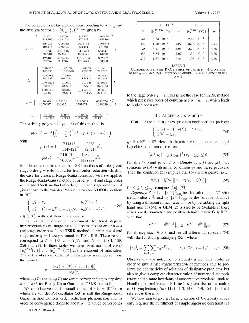
implementations of Runge-Kutta-Gauss method of order p = 4and stage order q = 2 and TSRK method of order p = 4 andstage order q = 4 are presented in Table II-B. These resultscorrespond to T = 2/3, h = T/N , and N = 32, 64, 128,256 and 512. In these tables we have listed norms of errors∥eRKG
h (T )∥ and ∥eTSRKh (T )∥ at the endpoint of integration
T and the observed order of convergence p computed fromthe formula
p =log(∥eh(T )∥/∥eh/2(T )∥
)log(2)
,
where eh(T ) and eh/2(T ) are errors corresponding to stepsizesh and h/2 for Runge-Kutta-Gauss and TSRK methods.
We can observe that for small values of ϵ (ϵ = 10−6) forwhich the van der Pol oscillator (53) is stiff the Runge-KuttaGauss method exhibits order reduction phenomenon and itsorder of convergence drops to about p = 2 which corresponds
ϵ = 10−6 ϵ = 10−6
N ∥eTSRKh (T )∥ p ∥eTSRK
h (T )∥ p
32 5.83 · 10−3 2.44 · 10−4
64 1.49 · 10−3 1.97 2.65 · 10−5 3.21
128 3.71 · 10−4 2.01 2.20 · 10−6 3.59
256 8.84 · 10−5 2.07 1.59 · 10−7 3.79
512 1.87 · 10−5 2.24 1.08 · 10−8 3.89
TABLE IICOMPARISON BETWEEN RKG METHOD OF ORDER p = 4 AND STAGE
ORDER q = 2 AND TSRK METHOD OF ORDER p = 4 AND STAGE ORDERq = 4
to the stage order q = 2. This is not the case for TSRK methodwhich preserves order of convergence p = q = 4, which leadsto higher accuracy.
III. ALGEBRAIC STABILITY
Consider the nonlinear test problem nonlinear test problem{y′(t) = g
(t, y(t)
), t ≥ 0,
y(0) = y0,(54)
g : R×Rd → Rd. Here, the function g satisfies the one-sidedLipschitz condition of the form(
g(t, y1)− g(t, y2))T
(y1 − y2) ≤ 0, (55)
for all t ≥ 0 and y1, y2 ∈ Rd. Denote by y(t) and y(t) twosolutions to (54) with initial conditions y0 and y0, respectively.Then the condition (55) implies that (54) is dissipative, i.e.,∥∥y(t2)− y(t2)
∥∥ ≤∥∥y(t1)− y(t1)
∥∥, (56)
for 0 ≤ t1 ≤ t2, compare [16], [73].Definition 3.1: Let {z[n]}Nn=0 be the solution to (2) with
initial value z[0], and by {z[n]}Nn=0 be the solution obtainedby using a different initial value z[0] or by perturbing the righthand side of (54). A GLM (2) is said to be G-stable if thereexists a real, symmetric and positive definite matrix G ∈ Rr×r
such that ∥∥z[n+1] − z[n+1]∥∥G≤∥∥z[n] − z[n]
∥∥G, (57)
for all step sizes h > 0 and for all differential systems (54)with the function g satisfying (55), where
∥z∥2G =
r∑i=1
r∑j=1
gijzTi zj , zi ∈ Rd, i = 1, 2, . . . , r. (58)
Observe that the notion of G-stability is not only useful inorder to give a nice characterization of methods able to pre-serve the contractivity of solutions of dissipative problems, butalso to give a complete characterization of numerical methodsretaining the same invariants of conservative problems, such asHamiltonian problems: this issue has given rise to the notionof G-symplecticity (see [15], [17], [48], [49], [54], [55] andreferences therein).
We now aim to give a characterization of G-stability whichonly requires the fulfillment of simple algebraic constraints in
INTERNATIONAL JOURNAL OF CIRCUITS, SYSTEMS AND SIGNAL PROCESSING Volume 11, 2017
ISSN: 1998-4464 439

place of (57), which is certainly hard to prove in general. Todo this, we provide the following definition.
Definition 3.2: The GLM (2) is said to be algebraicallystable, if there exist a real, symmetric and positive definitematrix G ∈ Rr×r and a real, diagonal and positive definitematrix D ∈ Rm×m such that the matrix M ∈ R(m+r)×(m+r)
defined by
M =
[DA+ATD−BTGB DU−BTGV
UTD−VTGB G−VTGV
](59)
is nonnegative definite.The significance of this definition follows from the resultproved by Butcher [14], that for preconsistent and non-confluent GLMs (2), i.e. methods with distinct abscissas ci,i = 1, 2, . . . ,m, algebraic stability is equivalent to G-stability.
It was observed by Hewitt and Hill [68], [69] that theverification if the matrix M is nonnegative definite can besimplified by the use of the following result proved by Albert[1].
Theorem 3.1: (Albert Theorem) The matrix M given by
M =
[M11 M12
MT12 M22
]satisfies M ≥ 0 if and only if
M11 ≥ 0, M22 −MT12M
+11M12 ≥ 0,
M11M+11M12 = M12,
(60)
or, equivalently,
M22 ≥ 0, M11 −M12M+22M
T12 ≥ 0,
M22M+22M
T12 = MT
12.(61)
Here, A+ stands for the Moore-Penrose pseudo-inverse of thematrix A.
Although the criteria based on Albert theorem can be usedto verify if specific examples of GLMs are algebraically stable,these criteria are not very practical to search for algebraicallystable GLMs which depend on some unknown parameters,unless some suitable simplifications are introduced. In fact, in[37], [69] the authors propose a simplified version of condi-tions (61), considering G = I and with some simplificationsin order to find algebraically stable TSRK methods whosecoefficients are expressed in rational form.
In [36], instead, an optimization-based numerical approachhas been used to derive the coefficients of algebraicallystable TSRK methods and two-step almost collocation (TSAC)methods, respectively. Because of the purely numerical natureof this approach, the coefficients of the corresponding methodsare not expressed in rational form, but they are provided witha certain number of correct digits. As a consequence, thederived methods satisfy a slightly weaker condition than that ofalgebraic stability, i.e. they are ε-algebraically stable methods.This concept has been introduced in [72], to which we referfor more details. The above mentioned approach is based onthe Nyquist stability function, defined by
N(ξ) = A+U(ξI−V)−1B, ξ ∈ C \ σ(V), (62)
where σ(V) stands for the spectrum of the matrix V. Adetailed explanation on the derivation of the Nyquist function
in the general setting of GLMs, together with its connectionswith control theory, can be found in [70], Section 5. Following[70], we denote by w a principal left eigenvector of V, i.e.the vector such that
wTV = wT , wTq0 = 1, (63)
where q0 is the preconsistency vector of GLMs. We nextdefine the diagonal matrix D by
D = diag(BT w), (64)
and by He(Q) the Hermitian part of a complex square matrixQ, i.e.,
He(Q) =1
2
(Q+Q∗),
where Q∗ stands for the conjugate transpose of Q. We havethe following result.
Theorem 3.2: (compare [14], [70]). A consistent GLM (2)is algebraically stable if the following conditions are satisfied:
1) the coefficient matrix V is power-bounded;2) Ux = 0 for all right eigenvectors of V and BTx = 0
for all left eigenvectors of V;3) D > 0 and DA ≥ 0;4) He
(DN(ξ)
)≥ 0 for all ξ such that |ξ| = 1 and ξ ∈
C \ σ(V).We now describe the construction of algebraically stable
TSRK methods belonging to the subclass of TSAC methods[51]. TSAC methods are continous methods of the form:P (tn + sh) = φ0(s)yn−1 + φ1(s)yn
+ hm∑j=1
(χj(s)f(P (tn−1 + cjh)) + ψj(s)f(P (tn + cjh))
),
yn+1 = P (tn+1),(65)
where tn = t0 + nh, n = 0, 1, . . . , N , Nh = T − t0, isa uniform grid. The continuous approximant P (tn + sh) isan algebraic polynomial which can be expressed as linearcombination of the basis functions
{φ0(s), φ1(s), χj(s), ψj(s), j = 1, 2, . . . ,m},
which are unknown algebraic polynomials to be suitablydetermined.
We observe that by evaluating the collocation polynomialat s = 1 and s = ci, i = 1, 2, . . . ,m, and by setting Y
[n]i =
P (tn + cih), i = 1, 2, . . . ,m, TSAC methods (37) can beformulated as TSRK methods
yn+1 = θyn−1 + θyn
+ hm∑i=1
(vif(Y
[n]i ) + wif(Y
[n−1]i )
),
Y[n]i = uiyn−1 + uiyn
+ hm∑j=1
(aijf(Y
[n]j ) + bijf(Y
[n−1]j )
),
(66)
where
θ = φ0(1), θ = φ1(1), vi = ψi(1), wi = χi(1),
ui = φ0(ci), ui = φ1(ci), aij = ψj(ci), bij = χj(ci),
INTERNATIONAL JOURNAL OF CIRCUITS, SYSTEMS AND SIGNAL PROCESSING Volume 11, 2017
ISSN: 1998-4464 440

i, j = 1, 2, . . . ,m. Observe that θ = 1−θ and ui = 1−ui, i =1, 2, . . . ,m
It is generally required that the polynomial P (tn + sh) in(65) satisfies the interpolation conditions
P (tn−1) = yn−1, P (tn) = yn, (67)
and the collocation conditions
P ′(tn−1 + cjh) = f(P (tn−1 + cjh)),
P ′(tn + cjh) = f(P (tn + cjh)),(68)
j = 1, 2, . . . ,m. However, in order to obtain methods withstrong stability properties such as, for example, A- or L-stability, we relax some of the interpolation and collocationconditions. This leads to additional free parameters which arethen used to obtain methods with desirable stability properties.Following the terminology introduced in [51] the resultingmethods are called TSAC methods.
Such methods are obtained by fixing ρ basis functionsamong the set
{φ0(s), χj(s), j = 1, 2, . . . ,m}, (69)
as polynomials of degree p = 2m + 1 − ρ, and deriving theremaining ones as solutions of the system of order conditions
φ0(s) + φ1(s) = 1,
(−1)k
k!φ0(s)+
+
m∑j=1
(χj(s)
(cj − 1)k−1
(k − 1)!+ ψj(s)
ck−1j
(k − 1)!
)=sk
k!,
(70)k = 1, 2, . . . , p. Then, it was proved in [51], that p = 2m +1− ρ is the uniform order of the resulting method.
In the paper [36] an algorithm was developed for thenumerical search of TSAC methods written as GLMs (2).This algorithm is based on minimizing the objective functionwhich computes the negative value of the minimum of theeigenvalues of the matrix
He(DN(ξ)), for ξ such that |ξ| = 1 and ξ ∈ C \ σ(V).(71)
Such matrix has been computed in [36] for TSAC methodsand assumes the form
He(DN(ξ)
)=
1
2(1 + θ)
(diag(v + w)
(A+
1
ξB
)+
(AT +
1
ξBT
)diag(v + w)
+
(ξ
(ξ − 1)(ξ + θ)+
ξ
(ξ − 1)(ξ + θ)
)vvT
+
(1
(ξ − 1)(ξ + θ)+
ξ
(ξ − 1)(ξ + θ)
)vwT
+
(ξ
(ξ − 1)(ξ + θ)+
1
(ξ − 1)(ξ + θ)
)wvT
+
(1
(ξ − 1)(ξ + θ)+
1
(ξ − 1)(ξ + θ)
)wwT
− 1
ξ + θ
((v + w) · u
)vT − 1
ξ + θv((v + w) · u)T
− 1
ξ(ξ + θ)
((v + w) · u
)wT − 1
ξ(ξ + θ)w((v + w) · u)T
).
Once order conditions are imposed and the other desiredproperties are achieved, the matrix (71) will depend on acertain number P of free parameters a1, a2, . . . , aP . Suchparameters will be chosen in order to satisfy condition 4 ofTheorem 3.2, i.e.
He(DN(ξ)
)∣∣∣ξ=eit
≥ 0, t ∈ [0, 2π], (72)
by means of the objective function
f(a1, a2, . . . , aP ) = −minj,k
λjk(a1, a2, . . . , aP ),
which is a numerical realization of the mentioned necessarycondition, where {λjk(a1, a2, . . . , aP ) : k = 1, 2, . . . . ,m} isthe spectrum of the matrix He
(DN(ei
2πn j)), j = 1, 2, . . . , n−
1, n ∈ N, being i the imaginary unit. We observe that wedid not consider the values j = 0 and j = n becausethey lead to points belonging to the spectrum of the matrixV. By increasing the number n of points on the unit circlewe search for methods satisfying (72), and the remainingnecessary conditions 1-3 in Theorem 3.2 for algebraic stabilityare verified on the case by case basis.
Since A-stable TSAC methods with m = 1, 2, 3 and p >m+1 have not been found in previous works (compare [51]),the search of algebraically stable methods has been performedamong TSAC methods of order p = m or p = m+ 1.
We now provide and example of method with m = 2 andp = 3. We carry out the search inside the class of A-stablemethods derived in [51]. Therefore, following [51], we imposethe interpolation conditions
φ0(0) = 0, χ1(0) = 0,
and we fix the ρ = 2 basis functions
φ0(s) = s(q2s
2 + q1s+ q0), χ1(s) = s
(r2s
2 + r1s+ r0),
INTERNATIONAL JOURNAL OF CIRCUITS, SYSTEMS AND SIGNAL PROCESSING Volume 11, 2017
ISSN: 1998-4464 441

where q2, q1, q0, r2, r1, and r0 are real parameters. We nextderive the values of these parameters realizing the collocationconditions
φ′0(c1) = φ′
0(c2) = 0 and χ′1(c1) = χ′
1(c2) = 0.
This leads to
q1 = − (c1 + c2)q02c1c2
, q2 =q0
3c1c2,
r1 = − (c1 + c2)r02c1c2
, r2 =r0
3c1c2.
We next determine the remaining basis functions φ1(s), χ2(s),ψ1(s), and ψ2(s) by imposing the system of order conditionsfor p = 3. As in [51], we fix c1 = 5/2 and c2 = 9/2. Thisleads to a two-parameter family of TSAC methods, dependingon q0 and r0. Within this family, we search for algebraicallystable methods, by minimizing the negative value of theobjective function computing the minimum of the eigenvaluesof the matrix (71). For instance, for
q0 = −0.4253608181543406, r0 = 1.6033382155047602,(73)
we obtain a method satisfying
He(DN(ξ))∣∣∣ξ=eit
≥ 0, t ∈ [0, 2π].
This bound has been obtained by dividing the interval [0, 2π]into n = 10000 subintervals.
IV. CONCLUSIONS
We described the construction of highly stable explicitand implicit GLMs. Namely, by using the IQS approach, wedescribed the construction of explicit GLMs of Nordsiek typehaving maximum area of the stability region, and A- and L-stablle implicit TSRK methods. We moreover presebnted theapproaches for the systematic search for algebraically stableGLMs for ODEs, based on the Albert theorem and the criteriaformulated by Hill, which are based on the Nyquist stabilityfunction. In all cases we presented example of methods. Fur-ther issues of this research will focus on analyzing nonlinearstability issues of numerical methods approximating otherfunctional operators such as integral and fractional equations[11], [21], [25], [33], [42], partial differential equations [26],[29]–[31], [39], [58], [61], oscillatory problems [40], [43],[59], [62], [65], [77].
REFERENCES
[1] A. Albert, Conditions for positive and non-negative definiteness in termsof pseudoinverses, SIAM J. Appl. Math. 17(1969), 434–440.
[2] Z. Bartoszewski and Z. Jackiewicz, Derivation of continuous explicittwo-step Runge-Kutta methods of order three, J. Comput. Appl. Math.205(2007), 764–776.
[3] Z. Bartoszewski, H. Podhaisky, and R. Weiner, Construction of stifflyaccurate two-step Runge-Kutta methods of order three and their contin-uous extensions using Nordsieck representation, Institut fur Mathamatik,Martin-Luther-Universitat Halle-Wittenberg, Reports on Numerical Math-ematics 01-2007.
[4] M. Bras. Nordsieck methods with inherent quadratic stability. Math.Model. Anal., 16(1), 82-96, (2011).
[5] M. Bras, A. Cardone, Construction of efficient general linear methods fornon-stiff differential systems, Math. Model. Anal. 17(2) (2012), 171–189.
[6] M. Bras, A. Cardone, R. D’Ambrosio, Implementation of explicit Nord-sieck methods with inherent quadratic stability, Math. Model. Anal. 18:2(2013) 289–307.
[7] Bras, M., Cardone, A., Jackiewicz, Z., Welfert, B. Order reductionphenomenon for general linear methods, Appl. Numer. Math. 119, 94–114. (2017).
[8] K. Burrage, High order algebraically stable multistep Runge-Kutta meth-ods, SIAM J. Numer. Anal. 24 (1987), no. 1, 106–115.
[9] Burrage, K. (1978). A special family of Runge-Kutta methods for solvingstiff differential equations. BIT 18, 22–41.
[10] Burrage, K., Butcher J.C., and Chipman F.H. (1980). An implementationof singly implicit Runge-Kutta methods. BIT 20, 326–340.
[11] Burrage, K., Cardone, A., D’Ambrosio, R., Paternoster, B., Numericalsolution of time fractional diffusion systems, Appl. Numer. Math. 116(2017), 82–94.
[12] Butcher, J.C. (1979). A transformed implicit Runge-Kutta method. J.Assoc. Comput. Mach. 26, 731–738.
[13] Butcher, J.C. (1987). The Numerical Analysis of Ordinary DifferentialEquations. Runge-Kutta and General Linear Methods, John Wiley & Sons,Chichester, New York.
[14] J.C. Butcher, The equivalence of algebraic stability and AN -stability,BIT 27(1987), 510–533.
[15] J. C. Butcher, Numerical methods for ordinary differential equations.John Wiley & Sons Ltd., Chichester, 2008.
[16] J.C. Butcher, Thirty years of G-stability, BIT 46(2006), 479–489.[17] Butcher, J., D’Ambrosio, R., Partitioned general linear methods for
separable Hamiltonian problems, Appl. Numer. Math. 117 (2017), 69–86.
[18] J.C. Butcher, Z. Jackiewicz, Diagonally implicit general linear methodsfor ordinary differential equations. BIT, 33(3) 452-472 (1993).
[19] J.C. Butcher, Z. Jackiewicz, Construction of general linear methods withRunge-Kutta stability properties. Numer. Algorithms, 36(1) 53-72, 2004.
[20] J. C. Butcher, Z. Jackiewicz and W. M. Wright. Error propagation ofgeneral linear methods for ordinary differential equations. J. Complexity,23(4-6) 560–580 (2007).
[21] G. Capobianco, D.Conte, I. Del Prete, High performance numericalmethods for Volterra equations with weakly singular kernels. J. Comput.Appl. Math. 228 (2009) 571-579.
[22] Cardone A., Conte D., Paternoster, B. A family of Multistep CollocationMethods for Volterra Integro-Differential Equations, AIP Conf. Proc.1168 (1), 358–361 (2009).
[23] A. Cardone, D. Conte, B. Paternoster, Two-step collocation methods forfractional differential equations, Discrete Contin. Dyn. Syst. Series B, toappear.
[24] Cardone A., Conte D., Multistep collocation methods for Volterraintegro-differential equations, Appl. Math. Comput. 221, 770–778 (2013).
[25] Cardone, A., D’Ambrosio, R., Paternoster, B., High order exponentiallyfitted methods for Volterra integral equations with periodic solution, Appl.Numer. Math 114 (2017), 18–29.
[26] Cardone, A., D’Ambrosio, R., Paternoster, B., Exponentially fittedIMEX methods for advection-diffusion problems, J. Comp. Appl. Math.316 (2017), 100–108.
[27] A. Cardone and Z. Jackiewicz, Explicit Nordsieck methods withquadratic stability, Numer. Algorithms 60, 1–25, (2012).
[28] A. Cardone, Z. Jackiewicz and H.D. Mittelmann. Optimization-basedsearch for Nordsieck methods of high order with quadratic stability. Math.Model. Anal. 17(3), 293–308, 2012.
[29] Cardone, A., Jackiewicz, Z., Sandu, A., Zhang, H., Extrapolation-based implicit-explicit general linear methods Numer. Algorithms, 65 (3),(2014) 377–399.
[30] Cardone, A., Jackiewicz, Z., Sandu, A., Zhang, H., ExtrapolatedImplicit-Explicit Runge-Kutta Methods, Math. Model. Anal. 19 (1),(2014) 18–43.
[31] A. Cardone, Z. Jackiewicz, A. Sandu, H. Zhang Construction of highlystable implicitexplicit methods Discrete Contin. Dyn. Syst., AIMS Pro-ceedings 2015 (2015), 185–194.
[32] A. Cardone, Z. Jackiewicz, J.H. Verner, B. Welfert, Order conditions forgeneral linear methods. J. Comput. Appl. Math. 290, 44–64 (2015).
[33] D. Conte, G. Capobianco, B. Paternoster, Construction and implemen-tation of two-step continuous methods for Volterra Integral Equations,Appl. Numer. Math. 119, 239-247 (2017).
[34] D. Conte, R. D’Ambrosio, G. Izzo, Z. Jackiewicz, Natural VolterraRunge-Kutta methods, Numer. Algor. 65 (3), 421–445 (2014).
[35] D. Conte, R. D’Ambrosio, Z. Jackiewicz, Two-step Runge-Kutta meth-ods with quadratic stability functions, J. Sci. Comput. 44, 191–218 (2010).
INTERNATIONAL JOURNAL OF CIRCUITS, SYSTEMS AND SIGNAL PROCESSING Volume 11, 2017
ISSN: 1998-4464 442

[36] D. Conte, R. D’Ambrosio, Z. Jackiewicz, and B. Paternoster, Numericalsearch for algebrically stable two-step almost collocation methods forordinary differential equations, J. Comput. Appl. Math. 239, 304–321(2013).
[37] D. Conte, R. D’Ambrosio, Z. Jackiewicz, and B. Paternoster, A practicalapproach for the derivation of two-step Runge-Kutta methods, Math.Model. Anal. 17(1), 65–77 (2012).
[38] D. Conte, R. D’Ambrosio, B. Paternoster, Two-step diagonally-implicitcollocation based methods for Volterra Integral Equations, Appl. Numer.Math. 62(10), 1312–1324 (2012).
[39] Conte, D., D’Ambrosio, R., Paternoster, B., GPU acceleration of wave-form relaxation methods for large differential systems, Numer. Algorithms71, 2 (2016), 293–310.
[40] D. Conte, E. Esposito, B. Paternoster, L. Gr. Ixaru,Some new uses ofthe ηm(Z) functions, Comput. Phys. Commun. 181, 128–137, 2010.
[41] D. Conte, Z. Jackiewicz, B. Paternoster, Two-step almost collocationmethods for Volterra integral equations, Appl. Math. Comput. 204(2008),839–853.
[42] D. Conte, B. Paternoster, Parallel methods for weakly singular VolterraIntegral Equations on GPUs, Appl. Numer. Math. 114,30-37 (2017).
[43] D. Conte, B. Paternoster, Modified Gauss-Laguerre exponential fittingbased formulae, J. Sci. Comput., 69 (1), 227-243 (2016).
[44] Conte, D. and Paternoster, B., A Family of Multistep CollocationMethods for Volterra Integral Equations, in Numerical Analysis andApplied Mathematics ed. by T. E. Simos, G. Psihoyios, Ch. Tsitouras;AIP Conference Proceedings 936, Springer, 2007, 128–131.
[45] D. Conte, B. Paternoster, Multistep collocation methods for Volterraintegral equations, Appl. Numer. Math. 59(2009), 1721–1736.
[46] D’Ambrosio, R., De Martino, G., Paternoster, B., Order conditions forGeneral Linear Nystrom methods, Numer. Algor. 65, 3 (2014) 579–595.
[47] D’Ambrosio, R., De Martino, G., Paternoster, B., General Nystrommethods in Nordsieck form: error analysis, J. Comput. Appl. Math. 292(2016), 694–702.
[48] D’Ambrosio, R., De Martino, G., Paternoster, B., A symmetric nearlypreserving general linear method for Hamiltonian problems, DiscreteContin. Dyn. Syst. (2015), 330–339.
[49] D’Ambrosio, R., De Martino, G., Paternoster, B., Numerical integrationof Hamiltonian problems by G-symplectic methods, Adv. Comput. Math.40, 2 (2014), 553–575.
[50] D’Ambrosio, R., Esposito, E., Paternoster, B. General linear methodsfor y”= f(y(t)), Numer. Algor. 61 (2), 331–349 (2012).
[51] R. D’Ambrosio, M. Ferro, Z. Jackiewicz, B. Paternoster, Two-stepalmost collocation methods for ordinary differential equations, Numer.Algorithms 53(2010), 195–217.
[52] D’Ambrosio, R., Ferro, M., and Paternoster, B., A General Family ofTwo Step Collocation Methods for Ordinary Differential Equations, AIPConf. Proc. 936, 2007, 45–48.
[53] D’Ambrosio, R., Ferro, M., and Paternoster, B., Collocation based twostep Runge–Kutta methods for Ordinary Differential Equations, in ICCSA2008 ed. by O. Gervasi et al.; Lecture Notes in Comput. Sci. 5073, PartII (2008), Springer, New York, 736–751.
[54] D’Ambrosio, R., Hairer, E., Zbinden, C., G-symplecticity impliesconjugate-symplecticity of the underlying one-step method, BIT Numer.Math. 53 (2013), 867–872.
[55] D’Ambrosio, R., Hairer, E., Long-term stability of multi-value methodsfor ordinary differential equations, J. Sci. Comput. 60, 3 (2014), 627–640.
[56] R. D’Ambrosio, Z. Jackiewicz, Continuous two-Step Runge-Kutta meth-ods for ordinary differential equations, Numer. Algorithms 54(2010),169–193.
[57] R. D’Ambrosio, Z. Jackiewicz, Construction and implementation ofhighly stable two-step continuous methods for stiff differential systems,Math. Comput. Simul. 81 (9), 1707-1728 (2011).
[58] D’Ambrosio, R., Moccaldi, M., Paternoster, B., Adapted numericalmethods for advection-reaction-diffusion problems generating periodicwavefronts, Comput. Math. Appl. 74, 5 (2017), 1029–1042.
[59] D’Ambrosio, R., Paternoster, B., Exponentially fitted singly diagonallyimplicit Runge-Kutta methods, J. Comput. Appl. Math. 263 (2014), 277–287.
[60] D’Ambrosio, R., Paternoster, B., A general framework for numericalmethods solving second order differential problems, Math. Comput.Simul. 110, 1 (2015), 113–124.
[61] D’Ambrosio, R., Paternoster, B., Numerical solution of reaction–diffusion systems of λ − ω type by trigonometrically fitted methods,J. Comput. Appl. Math. 294 (2016), 436–445.
[62] D’Ambrosio, R., Paternoster, B., Santomauro, G., Revised exponentiallyfitted Runge–Kutta–Nystrom methods, Appl. Math. Lett. 30 (2014), 56–60.
[63] R. D’Ambrosio, B. Paternoster, Two-step modified collocation methodswith structured coefficients matrix for Ordinary Differential Equations,Appl. Numer. Math. 62(10), 1325–1334 (2012).
[64] R. D’Ambrosio, B,. Paternoster, P-stable general Nystrom methods fory”=f(x,y), J. Comput. Appl. Math. 262, 271-280 (2014).
[65] Ixaru, L. Gr., Paternoster, B., A Gauss quadrature rule for oscillatoryintegrands, Comput. Phys. Comm. 133, 2–3 (2001), 177–188.
[66] E. Hairer, S. P. Nørsett and G. Wanner. Solving Ordinary DifferentialEquations I. Nonstiff Problems. Springer-Verlag, Berlin, Heidelberg, NewYork, 2000.
[67] E. Hairer and G. Wanner. Solving Ordinary Differential EquationsII. Stiff and Differential-Algebraic Problems, Second Revised Edition.Springer-Verlag, Berlin, Heidelberg, New York, 1996
[68] L.L. Hewitt and A.T. Hill, Algebraically stable general linear methodsand the G-matrix, BIT 49(2009), 93–111.
[69] L.L. Hewitt and A.T. Hill, Algebraically stable diagonally implicitgeneral linear methods, Appl. Numer. Math. 60(2010), 629–636.
[70] A.T. Hill, Nonlinear stability of general linear methods,Numer. Math.103(2006), 611–629.
[71] A.T. Hill, G-matrices for algebraically stable GLMs, Numer. Algorithms53(2-3), 281-292 (2010).
[72] G. Izzo and Z. Jackiewicz, Construction of algebraically stable DIM-SIMs, J. Comput. Appl. Math. 261, 77–84 (2014).
[73] Z. Jackiewicz, General Linear Methods for Ordinary Differential Equa-tions, John Wiley & Sons, Hoboken, New Jersey 2009.
[74] Z. Jackiewicz and S. Tracogna, A general class of two-step Runge-Kutta methods for ordinary differential equations, SIAM J. Numer. Anal.32(1995), 1390–1427.
[75] Z. Jackiewicz and S. Tracogna, Variable stepsize continuous two-step Runge-Kutta methods for ordinary differential equations, Numer.Algorithms 12 (1996), 347–368.
[76] Lambert, J.D. (1973). Computational Methods in Ordinary DifferentialEquations, John Wiley & Sons, Chichester, New York.
[77] Paternoster, B., Present state-of-the-art in exponential fitting. A contri-bution dedicated to Liviu Ixaru on his 70-th anniversary, Comput. Phys.Commun. 183 (2012), 2499–2512.
[78] A. Prothero, A. Robinson, On the stability and accuracy of one-stepmethods for solving stiff systems of ordinary differential equations. Math.Comput, 28(125) 145-162 (1974).
[79] Schur, J. (1916). Uber Potenzreihen die im Innern des Einheitskreisesbeschrankt sind. J. Reine Angew. Math. 147, 205–232.
[80] W.M. Wright, General linear methods with inherent Runge-Kutta stabil-ity, Doctoral thesis, The University of Auckland, New Zealand, 2002.
Angelamaria Cardone is researcher in NumericalAnalysis of University of Salerno, Italy. She receivedher PhD in Computational sciences and appliedmathematics in 2004, from University of NaplesFederico II, Italy. Her research interests regard thenumerical treatment of Volterra integral equations,ordinary differential equations and more recentlyfractional differential equations. Part of the researchdeals with the development of mathematical soft-ware, also in parallel environment.
Dajana Conte is Associate Professor in NumericalAnalysis at University of Salerno, Italy, since 2006.Her research activity concerns the development andanalysis of efficient and stable numerical methodsfor the solution of evolutionary problems, also withmemory, modeled by ordinary differential equa-tions and Volterra integral and integro-differentialequations. She was involved also on problems re-lated to the numerical solution of the many-bodySchrodinger equation in quantum molecular dynam-ics.
INTERNATIONAL JOURNAL OF CIRCUITS, SYSTEMS AND SIGNAL PROCESSING Volume 11, 2017
ISSN: 1998-4464 443

Raffaele D’Ambrosio is Associate Professor at theDepartment of Engineering and Computer Scienceand Mathematics of University of L’Aquila. He hasbeen Fulbright Research Scholar in the AcademicYear 2014-15 at Georgia Institute of Technology. Hisresearch topics mainly interest numerical methodsfor evolutionary problems of several kind (ordinaryand partial differential equations, integral equations,Hamiltonian problems, stochastic differential equa-tions, piecewise smooth dynamical systems), withparticular emphasis to structure-preserving numeri-
cal integration.
Beatrice Paternoster is Full Professor of Numeri-cal Analysis at University of Salerno, Italy. In herresearch she has been involved in the analysis andderivation of new and efficient numerical methodsfor functional equations, in particular differential andintegral Equations. She is also involved in parallelcomputation, with concerns to the development ofmathematical software for evolutionary problems.
INTERNATIONAL JOURNAL OF CIRCUITS, SYSTEMS AND SIGNAL PROCESSING Volume 11, 2017
ISSN: 1998-4464 444


![Numerical Bifurcation Analysis of Delay Differential ...kouzn101/engelborhgsTOMS.pdf · ysis]: Ordinary Differential Equations—multistep and multivalue methods; G.4 [Mathematical](https://static.fdocuments.in/doc/165x107/5f601a3c420b39090f45f192/numerical-bifurcation-analysis-of-delay-differential-kouzn101engelborhgstomspdf.jpg)