Stability Investigations in Power Systems

With The National Grid of the Sudan as A Special

Case

A thesis submitted

By

KAMAL RAMADAN DOUD B.Sc., M.Sc. (Electrical and Electronic Engineering)

University of Khartoum

In fulfillment of the Requirements for the Degree of Doctor of

Philosophy in Electrical and Electronic Engineering

Department of Electrical and Electronic Engineering

Faculty of Engineering and Architecture

University of Khartoum

May, 2004

ii

ACKNOWLEDGEMENTS

I would like to acknowledge that; the condition of this research would have

not been possible without the assistance and advice received from many great

people during the progress of the research.

I owe deep gratitude and appreciation to my co-supervisor Dr. A/Rahman

Ali Karrar who has patiently and continuously provided professional assistance

and guidance, and gave freely of his time and knowledge throughout the

condition of this work from the beginning till final review of the manuscript.

I am extremely thankful to my supervisor Dr. Al Amin Hamuda who has

continuously provided guidance and gave freely of his knowledge, experience

and time throughout the condition of this work.

In the development of the text of this research I am indebted to many

colleagues and friends and the Central Control Room at the National Electricity

Cooperation headquarters in Khartoum, for their advice and assistance both

with the material content and computation of the results included.

My thanks are also extended to my wife, friends who helped or encouraged

me during my study.

iii

ملخص البحث

يعتبر االتزان و التحكم في أنظمة القدرة الكهربائية من أهم المشاكل التي تواجه

تبر المسئول األول الهيئة القومية للكهرباء في السودان تع. التوسع في شبكات القدرة الكهربية

إلنتاج و توزيع القدرة الكهربية في العاصمة الخرطوم و معظم المدن الرئيسية في وسط

و لقد واجهت الهيئة مجموعة من مشاكل االتزان خالل توسعها المطرد في الحجم . السودان

هذه ازدادت. وكذلك من التعقيد الناتج من استمرارية اإلضافة لمحطات توليد و أحمال جديدة

المشاكل تعقيدا بعدم المعرفة الحقيقية لخواص الشبكة الفيزيائية و إليجاد حلول ناجعة قامت

الهيئة القومية للكهرباء بمجموعة دراسات لتقدير الحمل و التوليد المستقبلي على المدى القريب

غم من و البعيد و من ثم افترضت مجموعة حلول لتقوية الشبكة عند النقاط الضعيفة، و بالر

.ذلك ظلت مشكلة االتزان الدقيق قائمة باستمرارية زيادة الطلب على القدرة الكهربية

في هذه الدراسة تم بحث و عرض مشكلة االتزان بالتفصيل، و أيضا تم عرض و

تطبيق طرق جديدة اليجاد و تحليل قيم آيقن و استخدامها للتحكم في حساسية تذبذب اتزان

هذه الطرق ربطت بين المقدرة الحسابية للتحليل . حطات التوليد المتعددةاألنظمة ذات م

.الطورى لمصفوفة حالة الفضاء و التي يمكن الحصول عليها من الدالة االنتقالية للنظام

تم عرض معادالت و نمذجة خاصة لعناصر أنظمة القدرة الكهربية للحالة المستقرة ،

م تم كتابة مجموعة برامج باستخدام الحاسوب لتحليل و تحسين العابرة و المتحركة ومن ث

. طبقت هذه البرامج على شبكة السودان القومية للكهرباء. اتزان أنظمة القدرة الكهربية الدقيق

خلصت الدراسة بأن هذه البرامج ذات كفاءه عالية و تحتاج لحسابات قليلة مباشرة ويمكن

.ب شخصياستخدامها بسهولة في أي جهاز حاسو

أيضا قدمت الدراسة عده مقترحات لتحسين اتزان شبكة السودان القومية تغطى التوليد

.2006و الحمل الحالي و المستقبلي حتى عام

iv

Abstract

The stability and control of electrical power systems represent the most serious

problems, which may face the expansion of power systems. The National Grid of the

Sudan (N.G.), which supplies electricity to the Capital Khartoum and most of the

center towns, has faced many problems of stability during its continuous expantion in

size and complexity by adding new power stations or new loads. These problems have

been complicated by lack of real understanding of the system’s behavior. The

National Electricity Corporation of Sudan has carried out many studies to estimate

load forecasts for short and long term planning, and has suggested reinforcements for

the weak points of the system. But still the problems of small signal stability of the

N.G. remain especially as the demand increases continuously.

In this study the problem of small signal stability is presented and discussed in

details. Also, the study presents new techniques for the evaluation and interpretation

of eigen value sensitivity in the context of analysis and control of oscillatory stability

in multi-machine power system. These techniques combine the numeric power of

modal analysis of state-space models that can be obtained from system transfer

functions.

Certain models and equations for power system elements in the area of steady

state, transient and dynamic stability were presented and many computer programs

were written to analyse and improve small signal stability for any power system.

These studies were then applied to the N.G. of the Sudan. These programs were

efficient with straightforward formulation and less computation requirements and can

easily be implemented on any suitable personal computer.

The study, also, gives many suggestions to improve the stability of the N.G.

covering the existing and forecasting loads and generations up to 2006.

v

Contents Acknowledgements . . . . . . . . . . . . . . . . . . . . . . . . . . . . . . . . . . . . . . . . . . ii Arabic Abstract . . . . . . . . . . . . . . . . . . . . . . . . . . . . . . . . . . . . .. . . . . iii Abstract . . . . . . . . . . . . . . . . . . . . . . . . . . . . . . . . . . . . . . . . . . iv Contents . . . . . . . . . . . . . . . . . . . . . . . . . . . . . . . . . . . . . . . . . . v List of Figures . . . . . . . . . . . . . . . . . . . . . . . . . . . . . . . . . . . . . . . . . . x 1. Introduction . . . . . . . . . . . . . . . . . . . . . . . . . . . . . . . . . . . . . . . . . . . 1 2. Loadflow Models and Analysis 2.1 General Introduction . . . . . . . . . . . . . . . . . . . . . . . . . . . . . . . . . . . . . . . . . . . 5

2.2 Modeling for Steady State Stability Application . . . . . . . . . . . . . . . . . . . . 5

2.2.1 Introduction . . . . . . . . . . . . . . . . . . . . . . . . . . . . . . . . . . . . . . . . . . . 5

2.2.2 Synchronous Machine Steady State Model . . . . . . . . . . . . . . . . . . . . . . 6

2.2.3 Transformer Modeling . . . . . . . . . . . . . . . . . . . . . . . . . . . . . . . . . . 14

2.2.4 Transmission Line Modeling . . . . . . . . . . . . . . . . . . . . . . . . . . . . . 16

2.2.5 Load Models . . . . . . . . . . . . . . . . . . . . . . . . . . . . . . . . . . 19

2.3 Loadflow . . . . . . . . . . . . . . . . . . . . . . . . . . . . . . . . . . . . . . . . 22

2.3.1 Introduction . . . . . . . . . . . . . . . . . . . . . . . . . . . . . . . . . . . . . . . . 22

2.3.2 Loadflow Solution Techniques . . . . . . . .. . . . . . . . . . . . . . . . . . . . . 23

2.3.3 Description of the steady state stability digital program . . . . . . . . . . . 27

2.3.4 Comparison of Techniques . .. . . . . . . . . . . . . . . . . . . . . . . . . . . 28

3 Stability Tools and Methods

3.1 Introduction . . . . . . . . . . . . . . . . . . . . . . . . . . . . . . . . . . . . . . . . . . . . . . 41

3.2 Small Signal Stability Tools . . . . . . . . . . . . . . . . . . . . . . . . . . . . . . . . . . . . 41

3.2.1 State-Space Representation . . . . . . . . . . . . . . . . . . . . . . . . . . . . . . . . . . 41

3.2.2 Dynamic System Stability . . . . . . . . . . . . . . . . . . . . . . . . . . . . . . . . . . 43

3.2.2.1 Lyapunov’s First Method . . . . . . . . . . . . . . . . . . . . . . . . . . . . . . 46

3.2.2.2 Lyapunov’s Second Method [Direct Method] . . . .. . . . . . . . . . . 47

3.2.3 Eigenvalues and Eigenvectors . . . . . . . . . . . . . . . . . . . . . . . . . . . 47

3.2.4 Modal Matrices . . . . . . . . . . . . . . . . . . . . . . . . . . . . . . . . . . . . 48

3.3 Analysis of the Free Motion of a Dynamic System . . . . . . . . . . . . . . . . . . . 48

3.4 Mode Shape, Sensitivity and Participation Factor . . . . . . . . . . . . . . 51

3.4.1 Eigenvalue Sensitivity . . . . . . . . . . . . . . . . . . . . . . . . . . . . . . . . . . 52

3.4.2 Participation Factor . . . . . . . . . . . . . . . . . . . . . . . . . . . . . . . . . . . 52

vi

3.4.3 Controllability and Observability . . . . . . . . . . . . . . . . . . . . . . . . . . . . . 53

3.4.4 Relationship Between Eigenvalues and Transfer Function . . . . . . . . . . . 54

3.5 Small Signal Stability Theory . . . . . . . . . . . . . . . . . . . . . . . . . . . . . . . . 56

3.5.1 Analysis of a Single Machine Connected to Infinite bus System . . . . . 56

3.5.1.1 Generator Representation by The Classical Model . . . . . . . . . . 57

3.5.1.2 Single Machine Infinite Bus Including Field Circuit Dynamics . . . 61

3.6 Excitation System Model . . . . . . . . . . . . . . . . . . . . . . . . . . . . . . . . . . . . 64

3.7 State Equation for a Multi-machine System . . . . . . . . . . . . . . . . . . . . . . 67

3.7.1 Transformation Reference . . . . . . . . . . . . . . . . . . . . . . . . . . . . . . . . . . . 68

3.7.2 Procedure to form State Equation . . . . . . . . . . . . . . . . . . . . . . . . . . . . . 69

3.8 Procedure to form State Matrices . . . . . . . . . . . . . . . . . . . . . . . . . . . . . . 71

3.8.1 Algorithm to Find ∆X . . . . . . . . . . . . . . . . . . . . . . . . . . . . . . . . . . . . 72

3.8.2 Description of the Digital Program for Building and Analysis A . . . . 74

4 Improving The Stability Using Power system Stabilizer

4.1 Introduction . . . . . . . . . . . . . . . . . . . . . . . . . . . . . . . . . . . . . . . . . . . . . 78

4.2 PSS Theory and Modeling . . . . . . . . . . . . . . . . . . . . . . . . . . . . . . . . . . . 78

4.2.1 PSS Modeling . . . . . . . . . . . . . . . . . . . . . . . . . . . . . . . . . . . . . . . . . 81

4.2.2 PSS Design Approaches . . . . . . . . . . . . . . . . . . . . . . . . . . . . . . . . . . 86

4.2.2.1 Calculation of Transfer function Parameters . . . . . . . . . . . . . . 86

4.2.2.1.1 Classical Methods . . . . . . . . . . . . . . . . . . . . . . . . . . . . . 86

4.2.2.1.2 The New Designed Method . . . . . . . . . . . . . . . . . . . . 87

4.2.2.1.3 Updating the transfer function parameters . . . . . . . . . 90

4.3 Implementation of PSS . . . . . . . . . . . . . . . . . . . . . . . . . . . . . . . . . . . . 93

4.3.1 Implementation The Classical PSS . . . . . . . . . . . . . . . . . . . . . 93

4.3.2 Classical Method Robustness . . . . . . . . . . . . . . . . . . . . . . . . . 98

4.3.3 Implementation of the New Method . . . . . . . . . . . . . . . . . . . . . . 99

5 Improving The Stability Using Controlled Series Compensation

5.1 Introduction . . . . . . . . . . . . . . . . . . . . . . . . . . . . . . . . . . . . . . . . 103

5.2 System Modelling and Eigen values . . . . . . . . . . . . . . . . . . . . . . . . 103

5.3 Algorithm to Find ∆X . . . . . . . . . . . . . . . . . . . . . . . . . . . . . . . . . . . 105

5.4 Design of CSC Controllers for Multi-machine Systems . . . . . . . . . . . 109

5.4.1 Pole Placement Techniques . . . . . . . . . . . . . . . . . . . . . . . . . . . . . 109

5.4.2 Determination of the most effective location for a CSC . . . . . .. 109

vii

5.5 Description of CSC Digital Program for Dynamic Stability . . . . . . .. 110

6 Description of National Grid

6.1 General Introduction . . . . . . . . . . . . . . . . . . . . . . . . . . . . . . . . . . . . . . . 115

6.2 The Existing System . . . . . . . . . . . . . . . . . . . . . . . . . . . . . . . . . . . . . . . 115

6.2.1 Introduction . . . . . . . . . . . . . . . . . . . . . . . . . . . . . . . . . . . . . . . 115

6.2.2 Generation Plants . . . . . . . . . . . . . . . . . . . . . . . . . . . . . . . . . . . . . . . 118

6.2.2.1 Thermal Power Generation . . . . . . . . . . . . . . . . . . . . . . . . . 118

6.2.2.1.1 Khartoum North . . . . . . . . . . . . . . . . . . . . . . . . . . . . 119

6.2.2.1.2 Burri III Diesel Station . . . . . . . . . . . . . . . . . . . . . . 120

6.2.2.1.3 Kassala Diesel Station . . . . . . . . . . . . . . . . . . . . . . 120

6.2.2.1.4 Khashm El Girba Diesel Station . . . . . . . . . . . . . . . . 122

6.2.2.1.5 Kilo X Gas Turbine Station . . . . . . . . . . . . . . . . . . 122

6.2.2.1.6 Kuku Gas Power Station . . . . . . . . . . . . . . . . . . . 122

6.2.2.1.7 El-Gaili Gas Power Station . . . . . . . . . . . . . . . . . . . 123

6.2.2.2 Hydroelectric Power Generation . . . . . . . . . . . . . . . . . . . . . 123

6.2.3 Transmission Lines . . . . . . . . . . . . . . . . . . . . . . . . . . . . . . . . . . . 124

6.2.4 Reactors and Shunt Capacitors banks . . . . . . . . . . . . . . . . . . . . . . 126

6.2.5 Transformers . . . . . . . . . . . . . . . . . . . . . . . . . . . . . . . . . . . . . . . . 126

6.2.6 Off Grid Power Generation . . . . . . . . . . . . . . . . . . . . . . . . . . . . . 127

6.3 Control Systems Models and Practice . . . . . . . . . . . . . . . . . . . . . . . . . . 129

6.3.1 Introduction . . . . . . . . . . . . . . . . . . . . . . . . . . . . . . . . . . . . . . . . . 129

6.3.2 Generation Controllers . . . . . . . . . . . . . . . . . . . . . . . . . . . . . . . . . . 129

6.3.3 Automatic Voltage Regulators (AVR) . . . . . . . . . . . . . . . . . . . . 130

6.3.4 Governors . . . . . . . . . . . . . . . . . . . . . . . . . . . . . . . . . . . . . . . . . 130

6.3.5 Electrical Parameters . . . . . . . . . . . . . . . . . . . . . . . . . . . . . . . . . . 131

6.3.6 Relays . . . . . . . . . . . . . . . . . . . . . . . . . . . . . . . . . . . . . . . . . . . . . 131

6.3.6.1 Generation unit Relays . . . . . . . . . . . . . . . . . . . . . . . . . . . . 131

6.3.6.2 Transmission Line Relays . . . . . . . . . . . . . . . . . . . . . . . . 131

6.3.6.3 Transformer Relays . . . . . . . . . . . . . . . . . . . . . . . . 132

6.3.6.4 Busbar, Backup Protection and Auto-Reclosing units . . . . . . 132

6.4 Control Techniques and Problems in the N.G. . . . . . . . . . . . . . . . . . . 133

6.5 N.G. Loads and Problems . . . . . . . . . . . . . . . . . . . . . . . . . . . . . . . . . . 135

viii

6.6 Load Dispatch Center’s Operating Rules . . . . . . . . . . . . . . . . . . . . . . 136

7 Improving The Stability of The N.G.

7.1 Introduction . . . . . . . . . . . . . . . .. . . . . . . . . . . . . . . . . . . . . . . . . . . . . 138

7.2 Load and Operation Points Selection . . . . . . . . . . . . . . . . . . . . . . . . . 139

7.3 Improving The Stability of N.G. Using CSCs . . . . . . . . . . . . . . . . . . . 142

7.3.1 State Matrices and Eigen Values for N.G. . . . . . . . . . . . . . . . . . . . . 142

7.3.2 Improving The Poor Modes Using CSCs . . . . . . . . . . . . . . . . . . . . 145

7.3.3 Most effective Location for CSCs . . . . . . . . . . . . . . . . . . . . . . . . . 147

7.4 Improving the Poor Modes Using PSS . . . . . . . . . . . . . . . . . . . . . . . . 152

7.4.1 Improving the Stability Using Classical Model . . . . . . . . . . . . . . . 152

7.4.1.1 Selection of PSS model and its Parameters . . . . . . . . . . . . . 152

7.4.1.2 Analyzing N.G. for Three Load Modes . . . . . . . . . . . . . . . 152

7.4.2 Improving the Stability Using the New Designed PSS . . . . . . . . . . . 158

7.5 Transient Stability Studies . . . . . . . . . . . . . . . . . . . . . . . . . . . . . . . . . . . 162

7.5.1 Introduction . . . . . . . . . . . . . . . . . . . . . . . . . . . . . . . . . . . . . . . . . . 162

7.5.2 Study Results . . . . . . . . . . . . . . . . . . . . . . . . . . . . . . . . . . . . . . . . . 162

7.5.3 Comments on the Study Results . . . . . . . . . . . . . . . . . . . . . . . . . . . 163

8 Results and Conclusions 8.1 Results . . . . . . . . . . . . . . . . . . . . . . . . . . . . . . . . . . . . . . . . . . . . . . . . . . . 167

8.2 Recommendations . . . . . . . . . . . . . . . . . . . . . . . . . . . . . . . . . . . . . . . . . . 170

Refferences . . . . . . . . . . . . . . . . . . . . . . . . . . . . . . . . . . . . . . . . . . . . . . . 172

Appendices

I National Grid Data Base

I.A Existing Sub-stations for 220, 110 and 66 kV . .. . . . . . . . . . . . . . . . . . 183

I.B Transformer Data . . . . . . . . . . . . . . . . . . . . . . . . . . . . . . . . . . . . . . . . . 184

I.C Over Head Lines Technical Parameters for Power System Analysis . . 187

I.D Reactive Compensation Data . . . . . . . . . . . . . . . . . . . . . . . . . . . . . . 188

I.E Voltage Regulators . . . . . . . . . .. . . . . . . . . . . . . . . . . . . . . . . . . . . . 189

I.F Generator Data for Transient and Dynamic Stability Analysis . . . . . . 195

II Loadflow Results

II.A Light Load . . . . . . . . . . . . . . . . . . . . . . . . . . . . . . . . . . . . . . . . . . . . . . 197

II.B Medium Load . . . . . . . . . . . . . . . . . . . . . . . . . . . . . . . . . . . . . . . . . . 200

II.C Peak Load . . . . . . . . . . . . . . . . . . . . . . . . . . . . . . . . . . . . . . . . . . . 203

ix

II.D Light Load (2006) . . . . . . . . . . . . . . . . . . . . . . . . . . . . . . . . . . . . . . . . 206

II.E Peak Load (2006) . . . . . . . . . . . . . . . . . . . . . . . . . . . . . . . . . . . . . . . . . 210

III Calculation of the Partial Derivatives of Active and Reactive

Power with Respect to the Transformer off-Nominal Ratio . .. .. . . . . . 214

x

List of Figures

2.1 Operation Chart for a Cylindrical rotor Generator . . . . . . . . . . . . . . . . . . . 10

2.2 Operation Chart for a Salient-pole Generator . . . . . . . . . . . . . . . . . . . . . . . . . 11

2.3 Comparison between Stability Limits for a Salient-pole Machine with Xd = 1.1,

Xq= 0.7 p.u. and a Simplified Cylindrical Model with Xd = 1.1 p.u. . . . . . . . 12

2.4 Equivalent Circuit of an Off-Nominal 2-winding Transformer . . . . . . . . . . . . 16

2.5 Equivalent Circuit of a 3-winding Transformer .. . . . .. . . . . . . . . . . . . . . . . . 17

2.6 (a, b and c) Equivalent Circuit of an Off-Nominal 3-winding Transformer . . 18

2.7 Nine-busbar System Network . . . . . . . . . . . . . . . . . . . . . . . . . . . . . . . . . . . . . 29

2.8 (a) 9-busbar System Bus Voltage Results . . . . . . . . . . . . . . . . . . . . . . . . .. . 32

(b) 9-busbar System Active Power Results . . . . . . . . . . .. . . . . . . . . . . . .. . 33

(c) 9-busbar System Reactive Power Results . . . . . . . . . . . . . . . . . . . . . .. . 34

2.9 (a) N.G. Rosaries Hag Abdella Section . . . . . . . . . . . . . . . . . . . . . . . . . . 35

(b) N.G. Maringan-Kilo X Section . . . . . . . . . . . . . . . . . . . . . . . . . . . . . 36

(c) N.G. Khartoum Area Section . . . . . . . . . . . . . . . . . . . . . . . . . . . . . . 37

(d) N.G. Gaili Area Section . . . . . . . . . . . . . . . . . . . . . . . . . . . . . . . . . . 38

2.10 Loadflow Program Screen shot for N.G. . . . . . . . . . . . . . . . . . . . . . . . . . . . . 39

3.1 Equivalent Circuit for Single Machine connected to a large System . . . . . . . 56

3.2 Equivalent Circuit Using Classical Model . . . . . . . . . . . . . . . . . . . . . . . . . . 57

3.3 Block Diagram of Single Machine Infinite bus System . . . . . . . . . . . . . . . . . 59

3.4 Phasor Diagram Representation of the Dynamics of Rotor angle . . . . . . . . . 61

3.5 Block Diagram Representation with Constant Efd . . . . . . . . . . . . . . . . . . . . 63

3.6 Thyristor Exciter System with AVR . . . . . . . . . . . . . . . . . . . . . . . . . . . . . . . . 64

3.7 Block Diagram for the System with Exciter and AVR . . . . . . . .. . . . . . . . . . 66

3.8 Reference Frame Transformation . . . . . . . . . . . . . . . .. . . . . . . . . .. . . . . . . 68

4.1 Exciter and PSS Block Diagram . . . . . . . . . . . . . . . . . . . . . . . . . . . . . . . . . . . 78

4.2 The Reduced PSS Block Diagram . . . . . . . . . . . . . . . . . . . . . . . . . .. . . . . . . 79

4.3 PSS Single Block Diagram . . . . . . . . . . . . . . . . . . . .. . . . . .. . . . . . . . . . . . . 82

4.4 System 3-sub-Block Diagram . . . . . . . . . . . . . . . . . . . . . . . . . .. . . . . . . . . . 82

xi

4.5 State Space System with Feedback PSS . . . . . . . . . . . . . . . . . . . . . . . . . .. . . . 86

4.6 Direction for Increasing ζ at Constant ωn . . . . . . . . . . . . . . . . . . . . . . . . . .. . 88

4.7 Additional Feedback to the System . . . . . . . . . . . . . . . . . . . . . . . . .. . . . . . . 90

4.8 Bode Plot of PSS Transfer Function . . . . . . . . . . . . . . . . . . . . . . . . . .. . . . . 93

4.9 Bode Plot of the New Method Design . . . . . . . . . . . . . . . . . . . . . . . .. . . . . 101

6.1 Classical Model of the Generator . . . . . . . . . . . . . . . . . . . . . . . . . .. . . . . .. 116

6.2 Phasor Diagram for a Transient Synchronous Machine Model . . . . . . . . . 119

6.3 Five-Busbar System single line Diagram . . . . . . . . . . . . . . . . . . . . . . . . . . 126

6.4 Swing Curves for Machine 1 and 2 for clearing at 0.05s for the five-busbar

System . . . . . . . . . . . . . . . . . . . . . . . . . . . . . . . . . . . . . . . . . . . . . . . . . . . 128

6.5 Swing Curves for Machine 1 and 2 for clearing at 0.0225s . . . . . . . . . . . . 129

7.1 National Grid Existing Transmission Lines and Substations . . . . . . . . . . . . 136

8.1 Bode Plot for the New designed PSS for N.G. . . . . . . . . . . . . . . . . . . . . . . 176

8.2 National Grid Swing Curves for faults on the 33 kV level for Peak and Light

Load . . . . . . . . . . . . . . . . . . . . . . . . . . . . . . . . . . . . . . . . . . . . . . . . . . . . . . 181

xii

Chapter I Introduction

In recent years, among the electricity supply industry, there has been a growing

awareness of the need to maintain continuous balance between electrical generation

and varying load demand both in the steady state and when the system is subjected to

any form of disturbance. For power system frequency, voltage levels and security to

be maintained constant, a properly designed and operated power system should meet

the following fundamental requirements [1]; 1. The system must be able to meet the continually changing load demand for active and

reactive power, and withstand all types of disturbances. Since electricity can not be

conveniently stored in sufficient quantities, therefore, adequate spinning resource of

active and reactive power should be maintained and appropriately controlled at all times.

2. The system should supply energy at minimum cost and with minimum ecological impact.

3. The quality of power supply must meet certain minimum standards with regard to the

following factors;

a. Constancy of frequency

b. Constancy of voltage

c. Constancy of the level of reliability

On steady state operation, several levels of controls involving a complex array of

devices are used to meet the above requirements. But when the system is subjected to

any type of a sudden disturbance, the control devices must be able to make the system

survive the ensuring transient and move into an acceptable steady state condition and,

in this new steady-state condition all power components must be operating within

established limits. These disturbances or contingencies may be: 1. Sudden generator outages.

2. Load impact, rejection or addition.

3. Tripping of transmission lines or transformer.

4. Transient fault

The action of the control device before or after the contingency occurs would be

extremely limited if the contingency in question had not been foreseen and accounted

for in the planning studies that had been under-taken for the expansion and

reinforcement of the system.

xiii

Power system planning studies play the major role in the security of power systems.

The planning studies make use of the security analysis tools to simulate the various

types of contingencies on the system so as to make sure that the future performance of

the system would be reliable.

The power system stability problem is divided into three categories, depending on

the magnitude of the disturbance and the subsequent time interval of study, these are;

- Steady state stability

- Transient stability

- Dynamic stability

The models and tools used to analyze each of the 3-types differ widely to the

extent that each in its own right has become an independent area of research. To

enhance the general stability of the system the three types must be studied and the

findings integrated.

In Sudan, electricity is produced and distributed by the National Electrical

Corporation (NEC), which owns and operates the Sudanese network which is known

as National Grid (N.G.). The general topology of the N.G. is radial network since the

main hydro generation is centered at the remote South end (Roseries) and the bulk

load is at the center (Khartoum). There are other links at intermediate substations to

remote parts. This radial topology, as to be expected, causes a stability problem in the

operation of the N.G. The increase in load demand coupled with the limitation on

generation resources in the N.G. especially at the season of low hydro resources and

high demand of the year, has inflected on the grid a history of programmed and

unprogrammed sheddings. From the records of the blackout events on the N.G., it is

clear that there is a series problem of stability and security in the system of N.G.

NEC engineering staff has not been trained sufficiently to carry out studies that would

help in solving the problems of the system and suggesting its solutions.

The main objective of this study are, therefore, as follows:

1. To highlight and develop suitable models and mathematical equations to

analyse multi-machine power system networks operating in steady state,

transient or dynamic mode.

2. Convert the developed algorithms into software using a popular scientific

language such as MATLAB suitable for use in any PCs.

xiv

3. Analyse the power system dynamic behavior using state-variable

techniques to identify the poor mode of oscillations.

4. Investigate new approaches to improve poor modes of oscillation using

controlled series compensators (CSC).

5. Investigate new methods to design power system stabilizers (PSSs) and

use them to improve poor modes of oscillation.

6. Collect the electrical data of the N.G. in tabulated form suitable to be

analyzed using the developed software. Also to prepare lists containing

various modes for the existing and forecasting load conditions.

7. Carry out load flow studies on the N.G. using the selected load conditions.

8. Improve the stability of the N.G. using CSC and PSS

The subject material has been presented in 7 chapters, in addition to the

introduction and the final chapter (chapter 9) which covers the results and

conclusions. Additional notes are found in appendix I, II, III and a comprehensive

References list is included.

Chapter 2 develops models and common mathematical representations of power

system elements. Also in chapter 2 the steady state operation of power systems is

discussed and a visual load flow program is developed and verified in small network

examples and then extended to the analysis of large network such as N.G.

Chapter 3 outlines the problem of small signal stability and presents the stability

tools, models and mathematical equations. The chapter also introduces the formation

and use of state-variable matrices and eigenvalues in stability analysis. Chapter 4

presents the use of power system stabilizer PSS to improve the stability of power

system and develops new methods to design and calculate the parameters of the PSS.

Chapter 5 considers the introduction of controlled series compensator, (CSC), to

improve the stability of the system; also in chapter 5 a method is developed to build

the state matrix. This method overcomes the problem of the variable series reactance

of the CSC in the transmission line. Chapter 6 discusses the models and mathematical

equations of transient stability problem, and these models and equations are used to

develop a computer program coded in Matlab to analyse the transient stability of the

system. Furthermore, description of this program is given with it is applications.

Chapter 7 gives a full description of the National Grid of the Sudan; the existing

xv

facilities and the expected reinforcements. Additionaly, The electrical parameters for

generation, transmission lines, transformers and reactive compensators are tabulated

in the text and in appendix I.

Chapter 8 discusses the improvement of the N.G. dynamic oscillations using

CSCs and PSSs.

Finally chapter 9 presents the overall results and findings of the study and the

recommendations.

Chapter II Loadflow Models and Analysis

2.1 General Introduction

The power-flow (loadflow) analysis involves the calculation of power flows and

voltages of transmission lines for specified terminal or bus conditions. Such

calculations are required for analysis of steady-state as well as transient and dynamic

performance of power systems.

The system is assumed to be balanced; this allows a single-phase representation of

the system. For bulk power system studies, common practice is to represent the

composite loads as seen from bulk power delivery points [2] . Therefore, the effects of

distribution system voltage control devices on loads are represented implicitly.

In this chapter, the models for various elements of the power system are presented,

also a discussion of loadflow analysis as it applies to the steady state performance of

the power system is given. The basic network equations presented in this chapter also

apply to their representation in the analysis of system stability; however some of the

constraints vary depending on the type of the stability problem being solved.

xvi

2.2 Modeling for Steady State stability Application

2.2.1 Introduction

The formation of a mathematical model of a transmission network is a

prerequisite for power system analysis by digital computer. The form of the network

matrix used in the performance equation depends on the frame of reference, namely,

bus, branch or loop. In the bus representation the variables are the nodal voltages and

nodal currents whereas for the loop frame of reference the variables are loop voltages

and loop currents.

The use of the bus frame of reference greatly simplifies the preparation of data and

the shunted elements to ground may be included easily.

A power system is said to be steady-state stable for a particular operating

condition if, following any small disturbance, it reaches a steady state condition

which is identical or close to the pre – disturbance operating condition [2]. Voltage

stability, on the other hand, is the ability to maintain load voltage magnitudes within

specified operating limits under steady state condition [3]. Voltage stability problems

are particularly evident where electric power is transported over large distances from

remote power stations to the consumers.

Steady state stability for a complex power system is best investigated by

consideration of steady state stability limits within which the power system

components must remain constant as they would otherwise cause unstable conditions.

Having set limits on the operation of generating , transmission lines , transformers and

voltage level, it is possible to investigate steady state stability by adjusting the load of

the system by small increments and carrying out a load flow study for each

adjustment. This is repeated until a condition of instability is reached.

The important effects on steady state stability of voltage scheduling through

coordination of reactive power sources has been emphasized in literature [4]. In a

practical operation of a complex power system, gradually increasing the load will

result in operation of the on-load tap-changing transformers to compensate for the

accompanying voltage drop. Reactive power generation is increased by adjusting

generator excitations or by switching in static equipment either manually or

automatically. When all methods of compensation reach their limits, the system

voltage will fail to meet the stability requirements.

xvii

In the following sections, modeling aspects of power system equipment are

treated, with consideration given to the steady state operating limits in formulae that

are suitable for application using digital methods.

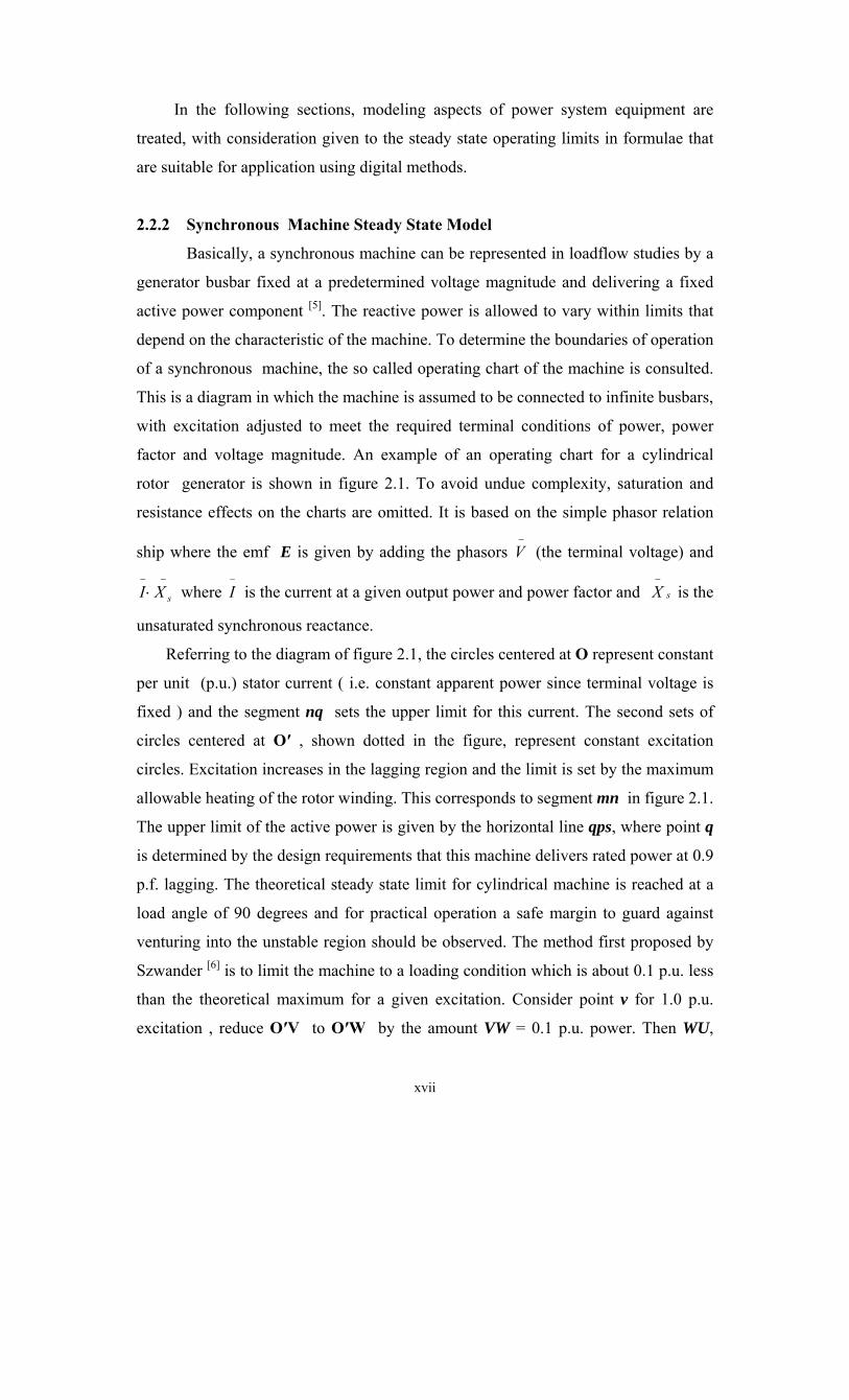
2.2.2 Synchronous Machine Steady State Model

Basically, a synchronous machine can be represented in loadflow studies by a

generator busbar fixed at a predetermined voltage magnitude and delivering a fixed

active power component [5]. The reactive power is allowed to vary within limits that

depend on the characteristic of the machine. To determine the boundaries of operation

of a synchronous machine, the so called operating chart of the machine is consulted.

This is a diagram in which the machine is assumed to be connected to infinite busbars,

with excitation adjusted to meet the required terminal conditions of power, power

factor and voltage magnitude. An example of an operating chart for a cylindrical

rotor generator is shown in figure 2.1. To avoid undue complexity, saturation and

resistance effects on the charts are omitted. It is based on the simple phasor relation

ship where the emf E is given by adding the phasors −

V (the terminal voltage) and −−

⋅ sXI where −

I is the current at a given output power and power factor and sX−

is the

unsaturated synchronous reactance.

Referring to the diagram of figure 2.1, the circles centered at O represent constant

per unit (p.u.) stator current ( i.e. constant apparent power since terminal voltage is

fixed ) and the segment nq sets the upper limit for this current. The second sets of

circles centered at O′ , shown dotted in the figure, represent constant excitation

circles. Excitation increases in the lagging region and the limit is set by the maximum

allowable heating of the rotor winding. This corresponds to segment mn in figure 2.1.

The upper limit of the active power is given by the horizontal line qps, where point q

is determined by the design requirements that this machine delivers rated power at 0.9

p.f. lagging. The theoretical steady state limit for cylindrical machine is reached at a

load angle of 90 degrees and for practical operation a safe margin to guard against

venturing into the unstable region should be observed. The method first proposed by

Szwander [6] is to limit the machine to a loading condition which is about 0.1 p.u. less

than the theoretical maximum for a given excitation. Consider point v for 1.0 p.u.

excitation , reduce O′V to O′W by the amount VW = 0.1 p.u. power. Then WU,

xviii

cutting the excitation circle U, fixes the point for which there is 0.1 p.u. power in

hand. The complete working area is mnqpsut.

For a salient pole alternator the difference is due to the values of Xd and Xq

(the direct and quadrature axis reactances). The operation chart for the salient pole

machine, which is shown in figure 2.2 is substantially the same as for the non-salient

machine except in the low excitation region. Due to saliency, the theoretically

stability limit occurs at angles which are less than 90° and which vary with excitation

as shown by the dotted curve in the diagram. The modification of the cylindrical rotor

chart for salient machines was described by Walker[7] and the practical stability limit

is constructed following the same steps proposed for the cylindrical machine with a

0.1 p.u. power margin. The boundary ut in the diagram is a restriction imposed by the

requirement that there shall always be a positive field excitation, since it is possible

for the machine to run with zero or slightly reversed excitation[8].

Generator operation should be confined to the region bounded by the limits

discussed above. The situation can be greatly simplified, particularly for computer

applications, by fitting the largest possible rectangle inside the operating region of

figure 2.1. In this case it is only necessary to provide three numbers, Qmin, Qmax and

Pmax to define the operating region. Alternatively, if greater accuracy is necessary for

the steady state boundary in the leading power region, which varies with the load,

then a simple formula for cylindrical machine can be defined as follows,

Reactive power delivered by the machine is given by,

dd X

VXEVQ

2

cos −= δ . . . . . . . . . . . . . . . . . . . . . . . . 2.1

the steady state stability limit is reached at δ = 90 and Q becomes

dX

VQ2

min−

= . . . . . . . . . . . . . . . . . . . . . . . . . . 2.2

if the machine is delivering P watts then

δsindX

EVP = . . . . . . . . . . . . . . . . . . . . . . . . . . . 2.3

at the theoretical steady state limit then

dX

EVP =′ . . . . . . . . . . . . . . . . . . . . . . . . . . . . 2.4

To provide a safe operating margin of, say, 0.1 p.u. of rated power then the working load

should be able to increase by 0.1 Prated before reaching the theoretical limit.

xix

Thus,

d

R XEVPP =+ 1.0 . . . . . . . . . . . . . . . . . . . . . . . . . . 2.5

substituting in equation 2.3

δsin)1.0( RPPP += . . . . . . . . . . . . . . . . . . . . . . . . . . 2.6

from which

201.02.0cos RR

d

PPPXEV

+=δ . . . . . . . . . . . . . . . . . 2.7

and hence equation 2.1 becomes

d

RR XVPPPQ

2201.02.0 −+= . . . . . . . . . . . . . . . . . . . . 2.8

Another way to arrive at this formula is to use the geometric relationships between points O′, W,

U, and V on figure 2.1. If equation 2.8 is plotted for different values of P it is seen that Q follows the

practical stability limit curve of figure 2.1 . The quantity V2/Xd is fixed and, since most machines are

specified in terms of their p.u. reactances and rated power then,

..

2

udp

rated

d X

MVA

XV

= . . . . . . . . . . . . . . . . . . . . . . 2.9

Equation 2.8 could be used in place of Qmin for computer application if increased accuracy is

judged necessary.

A salient-pole synchronous machine stability region can be approximated for computer studies by

that of a cylindrical machine and applying equation 2.9. The stability boundary in this case will be

somewhat stricter than the true boundary in the leading power factor region. Figure 2.3 compares the

operating boundaries for a salient pole machine with Xd =1.1 p.u. , Xq =0.7 p.u. with those of a

simplified model which takes into account only Xd.

xx

Fig 2.1 Operating chart for a cylindrical- rotor generator

xxi

Fig 2.2 Operating chart for a salient-pole generator

xxii

Fig 2.3 Comparison Between Stability Limits for a Salient-Pole

Machine with Xd = 1.1, Xq = 0.7 p.u. and a Simplified Cylindrical Model With Xd = 1.1 p.u.

2.2.3 Transformer Modeling

Transformers as modeled for steady state studies are either of the tap-changing or

non tap-changing type. Most power transformers are the former and the taps are

operated for voltage control purposes. Taps are changed by motor driven switches and

allowed to change on-load or off-load in a number of discrete steps above and below

nominal value (e.g. ±10%). A transformer which is operated in the off-nominal mode can be modeled for computer studies

as shown in figure 2.4 (b). This equivalent circuit is obtained by inserting an ideal transformer with an

off-nominal ratio a:1 (where a is real) in series with the transformer impedance as shown in figure 2.4

(a). This model is used extensively in power system loadflow studies. The transformer impedance is

assumed to remain constant irrespective of the tap position.

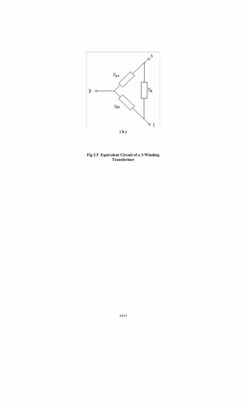
Three winding transformers with short circuit impedances Zps, Zpt, Zst calculated on a

common base are represented by the four node circuit shown in figure 2.5 (a) where,

xxiii

⎪⎭

⎪⎬

⎫

−+=

−+=

−+=

)(

)(

)(

21

21

21

psstptt

ptstpss

stptpsp

ZZZZ

ZZZZ

ZZZZ

. . . . . . . . . . . . . . . . . . . 2.10

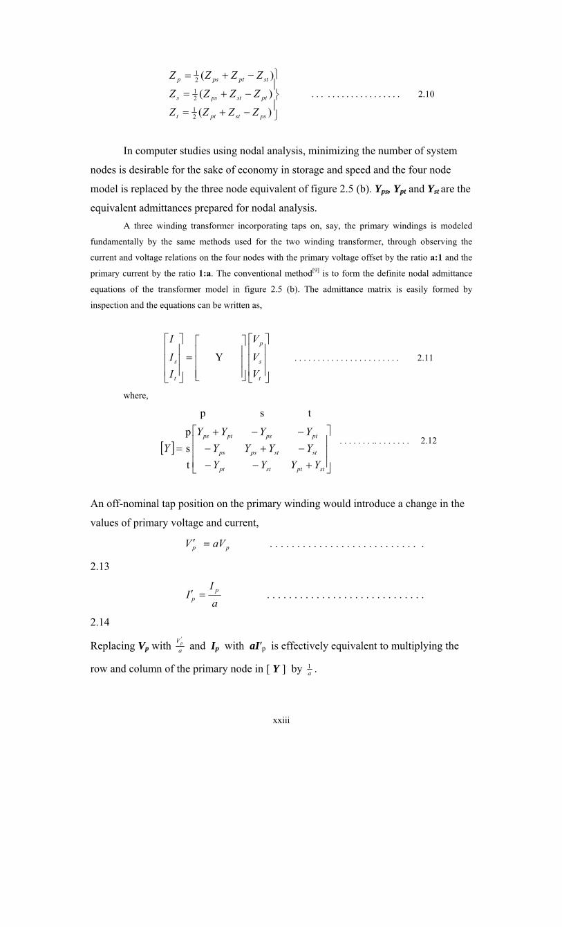
In computer studies using nodal analysis, minimizing the number of system

nodes is desirable for the sake of economy in storage and speed and the four node

model is replaced by the three node equivalent of figure 2.5 (b). Yps, Ypt and Yst are the

equivalent admittances prepared for nodal analysis. A three winding transformer incorporating taps on, say, the primary windings is modeled

fundamentally by the same methods used for the two winding transformer, through observing the

current and voltage relations on the four nodes with the primary voltage offset by the ratio a:1 and the

primary current by the ratio 1:a. The conventional method[9] is to form the definite nodal admittance

equations of the transformer model in figure 2.5 (b). The admittance matrix is easily formed by

inspection and the equations can be written as,

⎥⎥⎥

⎦

⎤

⎢⎢⎢

⎣

⎡

⎥⎥⎥

⎦

⎤

⎢⎢⎢

⎣

⎡=

⎥⎥⎥

⎦

⎤

⎢⎢⎢

⎣

⎡

t

s

p

t

s

VV

V

II

I

Y . . . . . . . . . . . . . . . . . . . . . . . 2.11

where,

[ ]⎥⎥⎥

⎦

⎤

⎢⎢⎢

⎣

⎡

+−−−+−−−+

=

stptstpt

ststpsps

ptpsptps

YYYYYYYYYYYY

Ytsp

t s p

. . . . . . . .. . . . . . . . 2.12

An off-nominal tap position on the primary winding would introduce a change in the

values of primary voltage and current,

pp aVV =′ . . . . . . . . . . . . . . . . . . . . . . . . . . . .

2.13

aI

I pp =′ . . . . . . . . . . . . . . . . . . . . . . . . . . . . .

2.14

Replacing Vp with aVp

'

and Ip with aI′p is effectively equivalent to multiplying the

row and column of the primary node in [ Y ] by a1 .

xxiv

[ ]

⎢⎢⎢⎢⎢⎢⎢

⎣

⎡

⎥⎥⎥⎥⎥⎥

⎦

⎤

+−−

−+−

−−+

=′

stptstpt

ststpsps

ptpsptps

YYYaY

YYYaY

aY

aY

aYY

t

s

p

Y

2

)( t s p

. . . . . . . . . 2.15

( note that the driving point admittance at node p is divided twice by a.)

It is possible to arrive at the same three node equivalent equations for a three winding off-

nominal transformer by making use of the equivalent circuit of an off-nominal two winding

transformer. Inserts an ideal transformer of ratio a:1 in series with the four node model of the three

winding transformer as shown in fig 2.6 (a) can immediately reduce the configuration to the one

shown in figure 2.6 (b).

The nodal admittance matrix for this configuration is then formed by inspection. Since node m

is fictitious with no current injection this node can be eliminated to arrive at the three node equivalent

admittance matrix [ Y′ ].

It is interesting to construct a model realizing matrix [ Y′ ] and figure 2.6 (c) shows this

realization. Representing the off-nominal three winding transformer in this way offers a physical

equivalent circuit parallel to that of the off-nominal two winding transformer. The similarities are

obvious and easily memorized.

The voltage at the consumers terminals is required by statute to remain within definite ranges

(±6% in Britain). Distribution transformers are thus regulated to meet the consumer requirements. The

steady state models for the transformers should account for the tap limits in both directions with respect

to the nominal position.

2.2.4 Transmission Line Modeling

Transmission lines are represented in steady state studies with sufficient accuracy by

equivalent π networks. The information generally required for each line is the positive sequence

resistance, inductance and shunt capacitance/km. Very long lines can be sectionalized to allow for a

more distributed account of their parameters. The problem of determining the power limits of a

transmission line has to take care of both steady state stability and thermal current ratings. A

transmission line will not be able to meet the voltage constraints at both ends if steady state stability

limit has been exceeded unless reactive compensation is introduced. Thermal current rating on the

other hand depends on the maximum conductor temperature allowable, ambient temperature, radiation

and convection heat losses.

xxv

( a )

( b )

Fig 2.4 Equivalent Circuit of an Off-Nominal 2-Winding Transformer

( a )

xxvi

( b )

Fig 2.5 Equivalent Circuit of a 3-Winding Transformer

xxvii

In general, for short lines the thermal current constraints prevail, whilst the stability limits

requirements are important for long lines.[10]

2.2.5 Load models

Peak loading and light loading conditions of power systems are useful in the assessment of the

steady state stability and voltage stability performance and loads are usually modeled by the active and

reactive power demands. Individual loads differ in characteristics but it is assumed that the active and

reactive power remain fixed and this assumption is found to be of reasonable accuracy when a large

number of the system busbar voltages are within 0.93 – 1.07 p.u.[11]

During stability assessment load are represent by their equivalent impedances. For transient

analysis load are represent by their pre-fault equivalent impedances.

( a )

xxviii

( b )

Fig 2.6 Equivalent Circuit of an Off-Nominal 3-Winding Transformer

xxix

Fig 2.6 ( c ) Three Node Equivalent of an Off-Nominal 3-Winding Transformer

2.3 Loadflow 2.3.1 Introduction The information sought during loadflow computation depends upon the particular application

and the types of measurements or input data available. In general nodal power conditions will

constitute the independent variables with nodal voltages as the dependent variables. Consequently the

determination of the nodal voltages, which initially appears to be elementary provided the nodal

currents are known, becomes a nonlinear problem requiring iterative solution since it is nodal power

rather than current is known.

Three types of nodes are usually considered to exist in a power network, namely the slack bus,

load buses and generation buses. The distinction is made on the basis of the data available at that node

and the classification is summarized in table 2.1

xxx

Bus type Known quantities Unknown quantities

Slack bus

Load bus

Generator bus

Voltage magnitude and

phase Real and reactive power

consumed

Voltage magnitude and Real

power generated

Real and reactive power

Voltage magnitude and

phase

Voltage angle and Reactive

power

Table 2.1 Node Classification

The loadflow problem therefore consists of determining the unknown quantities

in Table 2.1 together with the real and reactive power flow in the transmission lines

and transformers.

2.3.2 Loadflow Solution Techniques

The basic loadflow techniques used here in studying steady state performance is the well known

Newton-Raphson Method, which has powerful convergence properties. Studies which are performed

off-line can tolerate relatively slower execution times than on-line studies which are more suited to

decoupled or fast decoupled methods. In any case, the advantage of decoupled and fast decoupled

methods over the Newton-Raphson Method becomes considerably reduced for small systems[12].

There are some significant points to draw attention to in the present practice of dealing with

on-load tap changing transformers in iterative computer methods. If it is required, by changing the

transformer taps, to maintain the voltage at one side of the transformer constant, then it is necessary to

compensate for voltage drops by adjusting tap positions after each iteration. One method[13] is to treat

the controlled bus in the analysis as an ordinary load bus. The voltage of the bus V is checked at each

iteration against a specified voltage Vsp . The correction ( Vsp – V) is designated ∆V and the tap

adjustment ∆a is calculated as the integral multiple of tap steps closest to ∆V.

Another method[13] is to calculate the tap adjustment ∆a directly from the inversion of the

Jacobian matrix. This requires incorporation of the tap ratio a as a continuous variable in the power

equations of Newton’s method.

Treating a as a continuous rather than a discrete variable enables the use of the strong convergence

features of the method. The updated value of a at each iteration is adjusted to the nearest existing tap

position.

The Jacobian matrix is conventionally formed by taking the partial derivatives of the active

and reactive power with respect to the voltage and angle for load busbars (P–Q buses) and only the

active power with respect to the angle in the case of slack busbars (P–V buses). When it is desirable to

xxxi

maintain the voltage constant on one side of the transformer (normally the consumer side) by tap-

changer action then the active power and reactive power are both specified along with the specified

voltage and the off-nominal ratio a is treated as a variable. A designation ‘P-Q-V bus’ would be

suitable for this type of busbar. The Jacobian matrix equations for this busbar are formed as follows.

Let a two winding transformer with off-nominal ratio a:1 be connected between busbar i and j.

Also let busbar j be the transformer controlled busbar with voltage to be maintained at 1 p.u. ( see fig

2.4(a) & (b)).

Neglecting the transformer conductance gt then yt = jbt .

It can be shown that (see appendix III).,

⎪⎪

⎭

⎪⎪

⎬

⎫

−⋅⋅=∂

∂

−⋅⋅−=∂

∂

)cos(

)sin(

2

2

ijj

tij

j

j

ijj

tij

j

j

ab

VVaQ

ab

VVaP

δδ

δδ

. . . . . . . . . . .. . . . . . . . . . . . . 2.16

⎪⎪

⎭

⎪⎪

⎬

⎫

−−⋅⋅=∂

∂

−⋅⋅−=∂∂

32

2

2

2)cos(

)sin(

j

tiij

j

tji

j

j

ijj

tji

i

i

ab

Vab

VVaQ

ab

VVaP

δδ

δδ

. . . . . . . . . . . . . . . .. . 2.17

Similar equations can be derived for a three-winding transformer with the primary, secondary and

tertiary connected to nodes i, j and k respectively as follows. Let the tap side be the primary winding

and the controlled side at the secondary (node j).

With the conductances neglected,

Ypt = jbpt , Yst = jbst , Yps = jbps

And hence,

⎪⎪

⎭

⎪⎪

⎬

⎫

−⋅⋅=∂

∂

−⋅⋅−=∂

∂

)cos(

)sin(

2

2

ijj

psij

j

j

ijj

psij

j

j

a

bVV

aQ

a

bVV

aP

δδ

δδ

. . . . . . . . . . . . . . . . . . . 2.18

⎪⎪

⎭

⎪⎪

⎬

⎫

−⋅⋅=∂∂

−⋅⋅−=∂∂

)cos(

)sin(

2

2

ikj

ptik

j

k

ikj

ptik

j

k

a

bVV

aQ

a

bVV

aP

δδ

δδ

. . . . . . . . . . . . . . . . . . . . .. 2.19

xxxii

⎪⎪

⎭

⎪⎪

⎬

⎫

+−−⋅⋅−−⋅⋅=

∂∂

−⋅⋅−−⋅⋅−=∂∂

32

22

22

)(2)sin()cos(

)sin()sin(

j

ptpsiki

j

ptkiii

j

psji

j

i

kij

ptjiii

j

psji

j

i

a

bbV

a

bVV

a

bVV

aQ

a

bVV

a

bVV

aP

δδδδ

δδδδ

. . . .. 2.20

In order to assess the relative merits of the two methods of dealing with on-load

automatic tap-changers, two systems were selected and three studies were carried out

on each. The first system is the simple nine busbar network shown in figure 2.7, with

the line and transformer data given in table 2.2 and load and generation data in

table2.3. Busbar 4 was selected as the transformer controlled busbar. The second

system is the National Grid, of the Sudan, (N.G.) 110 busbar, basic configuration

system for the existing system up to March 2003, shown in figure 2.9. The line and

transformer data for this system can be found in appendix I and a typical loading

condition was selected for this study (see chapter VIII). For each system, transformer controlled busbars at which the voltage was to be maintained at Vsp

were adjusted by one of the following three methods;

1. treating the transformer controlled busbars as a load busbar with variable voltage V. The

off-nominal ratio is updated at each iteration as,

⎥⎦

⎤⎢⎣

⎡±

−∗+=+ 5.01

stepVV

INTstepaa spkk . . . . . . . . . . . . . . . . .. 2.21

where k stands for the iteration count, ‘step’ represents the magnitude of one tap

increment, and INT is a function that yields the integer value of the quantity enclosed in

brackets. The ‘+’ is used when V > Vsp and the ‘-‘ when V < Vsp. Tap adjustments stop

when the INT function yields zero for all transformers, and the iterations continue with

fixed tap positions until convergence is obtained. The process discontinues for a particular

transformer if it reaches either of its tap limits.

2. Treating the transformer controlled busbars as P-Q-V buses described in equations 2.1 –

2.5. The taps would ideally be updated at each iteration by computing ∆a by the method

which assumes smooth tap operation,

aaa kk ∆+=+1 . . . . . . . . . . . . . . . . . . . . . . . . . . . . . . . . . . 2.22

Instead, ak+1 is adjusted to the closest realizable value using,

⎥⎦

⎤⎢⎣

⎡±

∆∗+=+ 5.0)( '1

stepaINTstepaa kk . . . . . . . . . . . . . . . . . 2.23

xxxiii

Again this progress goes on until the adjustments diminish to zero for

all transformers and the control then switches to an ordinary loadflow

until convergence is obtained.

3. Using the previous method except that tap-changing is treated as a smooth

operation until a first convergence is obtained. Only then are the taps

adjusted to the nearest available positions and a second loadflow is carried

out with the tap settings fixed at these values.

All three methods gave identical results for the first system but whilst it took the

first two methods four iterations to arrive at the solution, the last method converged in

three iterations. The report and visual results of the loadflow study, for the first 9-

busbar system, are shown in table 2.4 and figure 2.8

The second and third method required a total of five iterations to arrive at a

solution for the National Grid system while the first method required ten iterations to

converge. The resulting reactive power distribution and tap positions of the first

method were slightly different from those of the second and third methods, which

were identical. Repeated trials with the two systems at different loading conditions indicated that method three

required the least number of iterations to obtain a solution, followed closely by method two, while the

convergence of the first method was comparatively slow.

2.3.3 Description of the steady state stability digital program

The program written for investigation of the steady state stability was coded in Microsoft

Visual Basic for use on any P.C. unit . The program essentially consists of three modules the main

routine, a network modification subroutine for performing system outages when a certain contingency

is selected and a network solution subroutine which performs the iterative process required to find a

solution .It is noteworthy to mention that the main routine is independent of the network solution

subroutine in the sense that any nodal analytical method can be used for the latter , whether the Gauss-

Siedal, Newton’s or decoupled algorithms.

Steady state performance is investigated by selecting a particular contingency, carrying out a

loadflow study, and detecting signs of steady state instability. This is done by scanning voltage levels

and line flows for violations of steady state limits. If convergence fails this is also taken as an

indication of steady state instability.

The program includes facilities to determine the reactive power requirements of a system

which is useful in planning for compensation reinforcements when the existing variable and static

compensation and tap-changing transformers are unable to maintain a reasonable voltage profile.

xxxiv

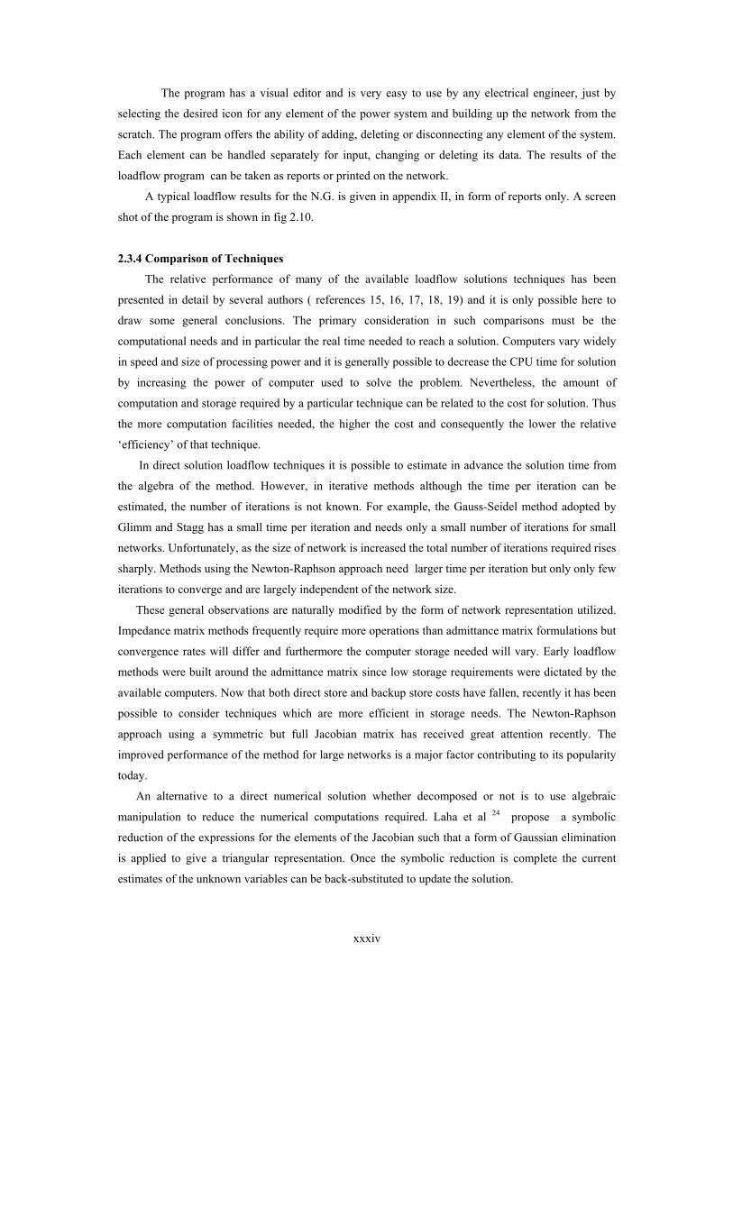
The program has a visual editor and is very easy to use by any electrical engineer, just by

selecting the desired icon for any element of the power system and building up the network from the

scratch. The program offers the ability of adding, deleting or disconnecting any element of the system.

Each element can be handled separately for input, changing or deleting its data. The results of the

loadflow program can be taken as reports or printed on the network.

A typical loadflow results for the N.G. is given in appendix II, in form of reports only. A screen

shot of the program is shown in fig 2.10.

2.3.4 Comparison of Techniques

The relative performance of many of the available loadflow solutions techniques has been

presented in detail by several authors ( references 15, 16, 17, 18, 19) and it is only possible here to

draw some general conclusions. The primary consideration in such comparisons must be the

computational needs and in particular the real time needed to reach a solution. Computers vary widely

in speed and size of processing power and it is generally possible to decrease the CPU time for solution

by increasing the power of computer used to solve the problem. Nevertheless, the amount of

computation and storage required by a particular technique can be related to the cost for solution. Thus

the more computation facilities needed, the higher the cost and consequently the lower the relative

‘efficiency’ of that technique.

In direct solution loadflow techniques it is possible to estimate in advance the solution time from

the algebra of the method. However, in iterative methods although the time per iteration can be

estimated, the number of iterations is not known. For example, the Gauss-Seidel method adopted by

Glimm and Stagg has a small time per iteration and needs only a small number of iterations for small

networks. Unfortunately, as the size of network is increased the total number of iterations required rises

sharply. Methods using the Newton-Raphson approach need larger time per iteration but only only few

iterations to converge and are largely independent of the network size.

These general observations are naturally modified by the form of network representation utilized.

Impedance matrix methods frequently require more operations than admittance matrix formulations but

convergence rates will differ and furthermore the computer storage needed will vary. Early loadflow

methods were built around the admittance matrix since low storage requirements were dictated by the

available computers. Now that both direct store and backup store costs have fallen, recently it has been

possible to consider techniques which are more efficient in storage needs. The Newton-Raphson

approach using a symmetric but full Jacobian matrix has received great attention recently. The

improved performance of the method for large networks is a major factor contributing to its popularity

today.

An alternative to a direct numerical solution whether decomposed or not is to use algebraic

manipulation to reduce the numerical computations required. Laha et al 24 propose a symbolic

reduction of the expressions for the elements of the Jacobian such that a form of Gaussian elimination

is applied to give a triangular representation. Once the symbolic reduction is complete the current

estimates of the unknown variables can be back-substituted to update the solution.

xxxv

xxxvi

Fig 2.7 Nine-busbar System Network

Line R(p.u.) X(p.u.) ωC/2(p.u.)

7 – 8 8 – 9 7 – 5 5 - 4 9 – 6 6 - 4

0.0085 0.0119 0.0320 0.0100 0.0390 0.0170

0.0720 0.1008 0.1610 0.0850 0.1700 0.0920

0.0745 0.1045 0.1530 0.0880 0.1790 0.0790

( a )

Transformer X(p.u.) Tap step Tap limits Upper Lower

1 – 7

2 – 9

3 - 4

0.0625

0.0586

0.0576

0.00375

0.00375

0.00375

1.045

1.045

1.045

0.955

0.955

0.955

xxxvii

( b )

Table 2.2 Line and Transformer Data for

Nine-busbar System

Bus Generation MWs MVArs

Load MWs MVArs

1 2 3 5 6 8

163 85 -

0.0 0.0 0.0

5.8 -10

- 0.0 0.0 0.0

0.0 0.0 0.0 125 90

100

0.0 0.0 0.0 50 30 35

Table 2.3 Load and Generation Data for

The Nine-busbar System

Load Flow Results ----------------------

Busbar Name Voltage Generation Load MW MVAr MW MVAr 1 sb 1.025< 9.3 163.0 6.7 0.0 0.0 2 gb 1.026< 3.7 0.0 0.0 0.0 0.0 3 gb 1.016< 0.7 0.0 0.0 100.0 35.0 4 1.032< 2.0 0.0 0.0 0.0 0.0 5 lb 1.025< 4.7 85.0 -10.9 0.0 0.0 6 lb 0.996< -4.0 0.0 0.0 125.0 50.0 7 lb 1.026< -2.2 0.0 0.0 0.0 0.0 8 lb 1.013< -3.7 0.0 0.0 90.0 30.0 9 lb 1.040< 0.0 71.6 27.0 0.0 0.0 Line Flows ----------- Between bus Sending End Receiving End MW MVAr MW MVAr 2 - 3 76.4 -0.8 -75.9 -10.7 4 - 3 24.2 3.1 -24.1 -24.3 2 - 6 86.6 -8.4 -84.3 -11.3 4 - 8 60.8 -18.1 -59.5 -13.5 8 - 7 -30.5 -16.5 30.7 1.0 6 - 7 -40.7 -38.7 40.9 22.9

2-Winding Transformer Flows

----------- Between Bus Primary Secondary MW MVAr MW MVAr 1 - 2 163.0 6.7 -163.0 9.2 5 - 4 85.0 -10.9 -85.0 15.0

xxxviii

9 - 7 71.6 27.0 -71.6 -23.9 Transmission Losses = 4.64MWs Number Of Iterations = 4 Where sb = slack bus gb = generator bus lb = load bus

Table 2.4 Nine-busbar System

Loadflow Results (report)

xxxix

Fig. 2.8-a 9-bus system Bus Voltage Results

Fig. 2.8-b 9-bus system Active Power Results

xl

Fig. 2.8-c 9-bus system Reactive Power Results

xli

Fig 2.9-a National Grid Basic Configuration System Roseries Section

xlii

Fig 2.9-b National Grid Basic Configuration System Kilo X Section

xliii

Fig 2.9-c National Grid Basic Configuration System

Khartoum North Section

Fig 2.9-d National Grid Basic Configuration System Gaili Section

xliv

Fig 2.10 Loadflow Program Screen Shot for Part of N.G.

Chapter III Stability Tools and Methods

3.1 Introduction

Small signal stability in power systems is the ability of the system to maintain synchronism

when subjected to small disturbances. The small disturbances are the ones that are described by

equations which can be linearized for the purpose of analysis. Instability that may arise due to such

disturbances can be of two forms[20]:

1. Steady increase in generator rotor angle due to lack of synchronizing torque.

xlv

2. Rotor oscillations of increasing amplitude due to lack of sufficient damping

torque.

In practical power systems, the small signal stability problem is usually one of

insufficient damping of oscillations.

This chapter discusses the fundamental aspects of the stability of dynamic systems

and presents analytical techniques and models useful in the study of small signal

stability.

3.2 Small Signal Stability Tools

3.2.1 State-Space Representation

The dynamic behavior of power systems can be described by a set of non-linear

ordinary differential equations of the form,

( ) nituuuxxxfx rnii ,,2,1,,,,;.,,, 2121 KKK& == . . . . . . . . . 3.1

where n is the order of the system

r is the number of inputs

Equation 3.1 can be written in vector matrix form as follows

),,( tuxfx =& . . . . . . . . . . . . . . . . . . . . . . . . . . . . . . . . 3.2

where

⎥⎥⎥⎥

⎦

⎤

⎢⎢⎢⎢

⎣

⎡

=

⎥⎥⎥⎥

⎦

⎤

⎢⎢⎢⎢

⎣

⎡

=

⎥⎥⎥⎥

⎦

⎤

⎢⎢⎢⎢

⎣

⎡

=

nrn f

ff

f

u

uu

u

x

xx

xMMM

2

1

2

1

2

1

,,

Here x is refered to as the state vector, and its entries xi as state variables. The column vector

u is the vector of the inputs to the system. t is the time and x• is the derivative, w.r.t time.

For non-explicit function of time, equation 3.2 can be written as,

),( uxfx =& . . . . . . . . . . . . . . . . . . . . . . . . . . . 3.3

The output of the system which are the parameters of interest, may be expressed as

),( uxgy = . . . . . . . . . . . . . . . . . . . . . . . . . . . 3.4

where

xlvi

⎥⎥⎥⎥

⎦

⎤

⎢⎢⎢⎢

⎣

⎡

=

⎥⎥⎥⎥

⎦

⎤

⎢⎢⎢⎢

⎣

⎡

=

mm g

gg

g

y

yy

yMM

2

1

2

1

,

where y is the output variables and g is a function state relating output and input variables.

The state-space of the system represents the minimum amount of information about the system at

any instant in the time domain t, that is necessary so that its future behavior can be determined without

reference to the input before to . Any set of n linearly independent system state variables may be used

to describe the state of the system. These state variables are the physical quantities such as angle,

speed, voltage or even the differential equation describing the dynamics of the system. Whenever the

system is not in equilibrium, or when the input is non-zero, the system state will change with time.

The equilibrium or singular points of the system are those which satisfy the equation,

0)( =oxf . . . . . . . . . . . . . . . . . . . . . . . . . . . . . 3.5

Where xo is the state vector x at the equilibrium point. If the functions in equation 3.3 are linear

then the system is linear; a linear system has only one equilibrium state.

3.2.2 Dynamic System Stability

The stability of a linear system is entirely independent of the inputs, and the state of a stable

system with zero input will always return to the origin of the state space, irrespective of the finite initial

state . In contrast, the stability of a non-linear system depends on the type and magnitude of input and

the initial state. These factors have to be taken into account in defining the stability of a non-linear

system.

In control system theory, it is common practice to classify the stability of a non-linear system into

the following categories depending on the region of state space in which the state vector ranges[20]:

1. Local stability or stability in the small

2. Finite stability

3. Global stability or stability in the large

The system is said to be locally stable about an equilibrium point if, when

subjected to small perturbation, it remains stable within a small region surrounding

the equilibrium point. And if the system returns to the original state, it is said to be

asymptotically stable in the small. If the system remains stable within a finite region

R, it is said to be stable within R. And further, if the system returns to the original

equation within R, it is asymptotically stable within the finite region R. The system is

said to be globally stable if R includes the entire finite space. Since xo and uo satisfy equation 3.3, where xo is the initial state vector and uo the input vector then,

xlvii

0),( == ooo uxfx . . . . . . . . . . . . . . . . . . . . . . . . . . 3.6

If the system is subjected to a perturbation then, x = xo + ∆x and u = uo + ∆u where ∆ denotes

small deviation. The new state must satisfy equation 3.3 . Hence

( ) ( )[ ]⎭⎬⎫

∆+∆+=

∆+=

uuxxf

xxx

oo

o

,&

&& . . . . . .. . . . . . . . . . . . . . 3.7

Since the perturbations are assumed small, the non-linear function f(x,u) can be expressed in

Taylor’s series expansion, ignoring second and higher order terms involving ∆x and ∆u, then

( ) ( )[ ]

( )⎪⎪⎪

⎭

⎪⎪⎪

⎬

⎫

∆∂∂

++∆∂∂

+∆∂∂

++∆∂∂

++=

∆+∆+=∆+=

rr

iin

n

iiooi

ooi

iioi

uuf

uuf

xxf

xxf

uxf

uuxxfxxx

LL

&&&

11

11

, . . . 3.8

since ),( ooioi uxfx =& then

rr

iin

n

iii u

uf

uuf

xxf

xxf

x ∆∂∂

++∆∂∂

+∆∂∂

++∆∂∂

=∆ LL& 11

11

. . . . . . .. 3.9

where i=1,2,. . . ,n

Similarly from equation 3.4,

rr

jjn

n

jjj u

ug

uug

xxg

xxg

y ∆∂

∂++∆

∂

∂+∆

∂

∂++∆

∂

∂=∆ LL 1

11

1

. . . . . . 3.10

or

⎭⎬⎫

∆+∆=∆∆+∆=∆

)()(

buDxCyauBxAx&

. . . . . . . . . . . . . . . . . . . . . . . 3.11

where

xlviii

⎪⎪⎪⎪⎪⎪⎪

⎭

⎪⎪⎪⎪⎪⎪⎪

⎬

⎫

⎥⎥⎥⎥⎥⎥

⎦

⎤

⎢⎢⎢⎢⎢⎢

⎣

⎡

∂∂

∂∂

∂∂

∂∂

=

⎥⎥⎥⎥⎥⎥

⎦

⎤

⎢⎢⎢⎢⎢⎢

⎣

⎡

∂∂

∂∂

∂∂

∂∂

=

⎥⎥⎥⎥⎥⎥

⎦

⎤

⎢⎢⎢⎢⎢⎢

⎣

⎡

∂∂

∂∂

∂∂

∂∂

=

⎥⎥⎥⎥⎥⎥

⎦

⎤

⎢⎢⎢⎢⎢⎢

⎣

⎡

∂∂

∂∂

∂∂

∂∂

=

r

mm

r

n

mm

n

r

nn

r

n

nn

n

ug

ug

ug

ug

D

xg

xg

xg

xg

C

uf

uf

uf

uf

B

xf

xf

xf

xf

A

L

MM

K

L

MM

K

L

MM

K

L

MM

K

1

1

1

1

1

1

1

1

1

1

1

1

1

1

1

1

,

,

. . . . . . . . . . . . . . 3.12

The A, B, C and D partial derivatives are evaluated at the equilibrium point about which the

small perturbation is being analyzed, and

∆x is the state vector of dimension n

∆y is the output vector of dimension m

∆u is the input vector of dimension r

A is the plant matrix of size n x n

B is the control or input matrix of size n x r

C is the output of size m x n

D is the feed-forward matrix which defines the probation of input which appears directly in output,

size m x r

In frequency domain, the Laplace transform of the above equation gives

)()()0()( suBsxAxsxs ∆+∆=∆−∆ . . . . . . . . . . . . . . . . . . . . . .. 3.13

)()()( suDsxCsy ∆+∆=∆ . . . . . . . . . . . . . . . . . . . . . . 3.14

A formal solution of the above equations can be obtained by solving for ∆x(s) and evaluating

∆y(s), as follows

From equation 3.13 (sI – A) ∆x(s) = ∆x(0)+B∆u(s) then

)]()0([)()( 1 suBxAsIsx ∆+∆−=∆ −

Hence

[ ])()0()det()()( sBux

AsIAsIadjsx +∆

−−

=∆ . . . . . . . . . .. . . . 3.15

And correspondingly

[ ] )()()0()det()()( suDsuBx

AsIAsIadjCsy ∆+∆+∆

−−

=∆ . . . . . . . . . . . 3.16

xlix

From equation 3.15 and 3.16, ∆x and ∆y are seen to have two components, one dependant on the

initial conditions and the other on the inputs.

The poles of ∆x(s) and ∆y(s) are the roots of the equation

0)det( =− AsI . . . . . . . . . . . .. . . . . . . . . . . . . . . . . 3.17

The values of s which satisfy equation 3.17 are known as the eigen-values of matrix A, and

equation 3.17 is referred as the characteristic equation of matrix A. Lyapunov described the following

two methods for testing the stability of the system using eigen-values.

3.2.2.1 Lyapunov’s First Method

The stability in small of a non-linear system is given by the roots of the

characteristic equation of the system of first approximation ( i.e. by eigenvalues of A)

as follows[20],

1. When the eigenvalues have negative real parts, the original system is

asymptotically stable.

2. When at least one of the eigenvalues has positive real part, the original system

is unstable. 3. When the eigenvalues have real parts equal to zero it is not possible on the basis of the first

approximation to say anything in general.

3.2.2.2 Lyapunov’s Second Method [Direct method]

Here the stability is determined directly by using suitable functions which

are defined in the state space. The equilibrium of equation 3.3 is stable if there exists a positive definite function V(x1,x2, . . . ,xn)

such that its total derivative V ْ with respect to equation 3.3 is not positive.

The equation of 3.3 is asymptotically stable if there is a positive definite function V(x1,x2, . . . ,xn)

such that its total derivative with respect to equation 3.3 is negative definite. The system is stable in the

region in which V ْ is negative semidefinite, and asymptotically stable if V ْ is negative definite.

3.2.3 Eigenvalues and Eigenvectors

The eigenvalues for a matrix A are the scalar parameters λ which satisfy the solution of equation

φλφ =A . . . . . . . . . . . . . . . . . . . . . . . . . . . . . . . . .. 3.18

or

( ) 0=− φλ IA . . . . . . . . . . . . . . . . .. . . . . . . . . . . . . . . . 3.19

l

where φ ≠ 0 and A is an n x n matrix describing a power system.

φ is an n x 1 vector matrix

For a non-trivial solution det( A - λ I ) = 0 , expanding this determinant gives the characteristic

equation, and the n – solution of λ, eigen values, are λ1, λ2, . . . . , λn

For any eigenvalue λi the n-column vector φi which satisfies equation 3.18 is called the right

eigenvector of A, associated with the eigenvalue λi . So,

niA iii ,,2,1, L== φλφ . .. . . . . . . . . . . . . . . . 3.20

The eigenvector φi has the form

⎥⎥⎥⎥

⎦

⎤

⎢⎢⎢⎢

⎣

⎡

=

ni

i

i

i

φ

φφ

φM

2

1

Similarly, the n-row vector Ψi which satisfies the equation

niA iii ,....,2,1, == ψλψ . .. . . . . . . . . . . . . . . . . . . 3.21

is called the left eigenvector associated with the eigenvalue λi .

It is common practice to normalize the vector φ and Ψ

1=iiφψ . . . . . . . . . . . . . . . . . . . . . . . . . . . . . 3.22

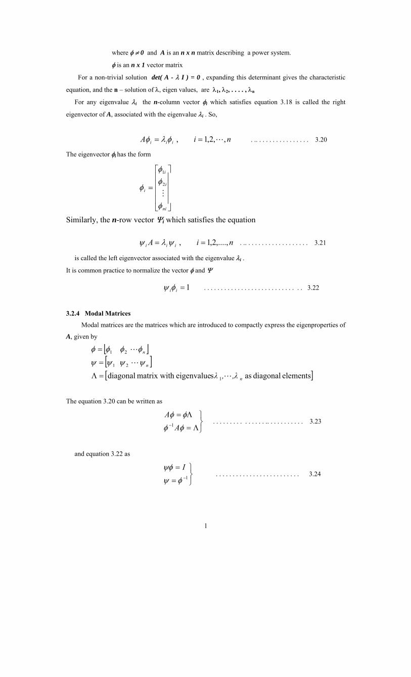
3.2.4 Modal Matrices

Modal matrices are the matrices which are introduced to compactly express the eigenproperties of

A, given by

[ ][ ][ ]elements diagonal as seigenvalueh matrix wit diagonal 1

21

21

n

n

n

,λ,λ L

L

L

=Λ

=

=

ψψψψ

φφφφ

The equation 3.20 can be written as

⎭⎬⎫

Λ=

Λ=− φφ

φφ

AA

1 . . . . . . . . . . . . . . . .. . . . . . . . . . . 3.23

and equation 3.22 as

⎭⎬⎫

=

=−1φψ

ψφ I . . . . . . . . . . . . . . . . . . . . . . . . . 3.24

li

3.3 Analysis of the Free Motion of a Dynamic System

For a free motion ( zero input) equation 3.11(a) is given by[20]

xAx ∆=∆& . . . . . . . . . . . . . . . . . . . . . . . . . . . 3.25

In order to eliminate the cross-coupling between the state variables, a new state vector z related to

the original state vector ∆x is defined by the transformation

zx φ=∆ . . . . . . . . . . . . . . . . . . . . . . . . . . . . . 3.26

substituting equation 3.26 into equation 3.25 gives,

zAz φφ =& . . . . . . . . . . . . . . . . . . . . . . . . . . . . . 3.27

so

zAz φφ 1−=& . . . . . . . . . . . . . . . . . . . . . . . . . . . . . 3.28

and using equation 3.23

zz Λ=& . . .. . . . . . . . . . . . . . . . . . . . . . . . . . . . 3.29

the last equation represents n uncoupled first order equations given by,

nizz iii ,,2,1, L& == λ . . . . . . . . . . . . . . . . . 3.30

Equation 3.30 has a solution in time domain given by,

t

iiieztz λ)0()( = . . . . . . . . . . . . . . . . . 3.31

Where zi(0) is the initial value of zi .

The response in terms of the original state vector can be found from equation 3.26 as,

[ ]

⎪⎪⎪

⎭

⎪⎪⎪

⎬

⎫

⎥⎥⎥⎥

⎦

⎤

⎢⎢⎢⎢

⎣

⎡

=

=∆

)(

)()(

)()(

2

1

21

tz

tztz

tztx

n

nM

Lφφφ

φ

. . . . . . . . . . . . . . . . . . . . . . . . . 3.32

or

∑=

=∆n

i

tii

ieztx1

)0()( λφ . . . . . . . . . . . . . . . . . . . . . . . . . 3.33

from equation 3.24 and 3.32

⎭⎬⎫

∆=∆= −

)()()( 1

txtxtz

ψφ

. . . . . . . . . . . . . . . . . . . . . . . . . 3.34

lii

hence

)()( txtz ii ∆=ψ . . . . . . . . . . . . . . . . . . . . . . . . . 3.35

at t =0, it follows that

)0()0( xz ii ∆=ψ . . . . . . . . . . . . . . . . . . . . . . . . . 3.36

putting ci = ψi ∆x(0) then

∑=

=∆n

i

tii

iectx1

)( λφ . . . . . . . . . . . . . . . . . . . . .. . . 3.37

or in the i-th state variables is given by t

nint

it

iinececectx 121

2211)( λλλ φφφ +++=∆ L . . . . . 3.38

This equation gives the expression for the free motion time response of the system in terms of the

eigenvalues and the left and right eigenvectors. Thus, the free response is given by the linear

combination of n dynamic modes corresponding to n eigenvalues of the state matrix.

If the initial conditions lie along the j-th eigenvector, the scalar products ψi∆x(0) for all i ≠ j are

identically zero. Therefore only the j-th mode exists.

The time response corresponding to an eigenvalue λi is given by eλit , therefore the stability of the

system is determined by eigenvalues as follows [20]:

1. A real eigenvalue corresponds to a non-oscillatory mode. A negative real

eigen value represents a decaying mode, the larger its magnitude, the faster

the decay. A positive real eigenvalue represents periodic instability. 2. Complex eigen-values occur in conjugate pairs, and each pair corresponds to an oscillatory

mode. The real component of the eigenvalues gives the damping, and the imaginary

component gives the frequency of oscillation. A negative real part represents a damped

oscillation whereas a positive real part represents oscillation of increasing amplitude.

Thus for complex pair of eigenvalues,

ωσλ j±= . . . . . . . . . . . . . . . . . . . . . 3.39

The frequency of oscillation in Hz is given by

πω2

=f . . . . . . . . . . . . . . . . . . . . . . . . . . . . . 3.40

and the damping ratio is given by,

liii

22 ωσ

σξ+

−= . . . . . . . . . . . . . . . . . . . . . . . . . 3.41

The damping ratio determines the ratio of decay of the amplitude of oscillation.

The time constant of amplitude decay is σ1 .

3.4 Mode Shape, Sensitivity and Participation Factor

The relationship between ∆x and z is given by equation,

⎭⎬⎫

∆==∆

)()()()()()(

btxtzatztx

ψφ

. . . . . . . . . . . . . . . . 3.42

Where ∆x is the vector of the original state variable representing the dynamic performance of the

system and z is the transformed state variable. From equations 3.42 (a) and (b), the k-th element of the

right eigenvector φi measures the activity of the variable xk in the i-th mode and the k-th element of the

left eigenvector ψi weights the contribution of this activity to the i-th mode.

3.4.1 Eigenvalue Sensitivity

Differentiating equation 3.18, which defines the eigenvalues and eigenvectors with respect to akj

the element of A in the k-th row and j-th column yields,

kj

iii

kj

i

kj

ii

kj aaaA

aA

∂∂

+∂∂

=∂∂

+∂∂ φ

λφλφ

φ

multiplying by ψi ,

kj

ii

kji aa

A∂∂

=∂∂ λ

φψ

notice ψiφi = 1 and ψi ( A - λi I ) = 0

so all elements of kja

A∂∂

are zeros, except for the elements in the k-th row and j-th column

which are equal to 1, hence

jiikkj

i

aφψ

λ=

∂∂

. . . . . . . . . . . . . . . . . . . . . . . . 3.43

Thus the sensitivity of the eigenvalue λi to the element akj of the state matrix is equal to the

product of the left eigenvector element ψik and the right eigenvector element φji .

liv

3.4.2 Participation Factor

The elements of eigen vectors are dependent on units and scaling associated with the state

variables, so that a problem arises when using the right and left eigenvector individually for identifying

the relationship between the states and modes[20]. To solve this problem the participation matrix (P) is

used, which combines the right and left eigenvector as follows,

[ ]nPPPP L21= . . . . . . . . . . . . . . . . . . . . . 3.44

with

⎥⎥⎥⎥

⎦

⎤

⎢⎢⎢⎢

⎣

⎡

=

⎥⎥⎥⎥

⎦

⎤

⎢⎢⎢⎢

⎣

⎡

=

inni

ii

ii

ni

i

i

i

P

PP

P

ψφ

ψφψφ

MMM

22

11

2

1

. . . . . . . . . . . . . . . . . . . . . . 3.45

This is used as a measure of association between the state variables and modes, where

φki = the element on the k-th row and i-th column on the modal matrix φ

ψik = the element on the i-th row and k-th column of the modal matrix ψ

The element Pki = φkiψik is termed the participation factor[21]. It is a measure of the relative

participation of the k-th state variable in the i-th mode, and vice versa. The multiplication of elements

of the left and right eigenvectors is also to make Pki dimensionless.

From equation 3.43 it is clearly seen that the participation factor Pki is actually equal to the

sensitivity of the eigen value λi to the diagonal element akk of the state matrix A

kk

iki a

P∂∂

=λ

. . . . . . . . . . . . . . . . . . . . . . . . . . . .. . 3.46

3.4.3 Controllability and Observability

Equation 3.8 and 3.9 can be expressed in terms of z by

uDCyuBAz

z

z

∆+=∆∆+=

φφφ &

or

uBAzz ∆′+=& . . . . . . . . . . . . . . . . . . . . . . . . . 3.47

uDzCy ∆+′=∆ . . . . . . . . . . . . . . . . . . . . . . . . . 3.48

where

B′ =φ-1B

C′ = Cφ

lv

From equation 3.47, if the i-th row of matrix B′ is zero the inputs have no effect on the i-th mode. In

such a case, the i-th mode is said to be uncontrollable. From equation 3.48, it is seen that the i-th

column of matrix C′ determines whether or not the variable zi contributes to the formation of the

outputs. If the column is zero, then the corresponding mode is unobservable. So the n x r matrix B′ =

φ-1B is known as mode controllability matrix, and the m x n matrix C′ = Cφ as mode observability

matrix [22]. (r = the number of inputs, m = number of outputs).

3.4.4 Relationship Between Eigenvalues and Transfer Function

The state representation of a system is a complete description of the system and it is ideally suited

for analysis of multi-variable, multi-input and multi-output system. For small signal stability, the

analysis depends primarily on the eigenvalues of the system state matrix. For control design, the

parameter of interest is the open loop transfer function between specific variables.

Equation 3.11(a) and (b) can be written as,

ubxAx ∆+∆=∆& . . . . . . . . . . . . . . . . . . . . . . . . 3.49

xCy ∆=∆ . . . . . . . . . . . . . . . . . . . . . . . 3.50

Where A is the state matrix, ∆x is the state vector, ∆u is a single input, ∆y is a single output , C is a

row vector and b is a column vector (D = 0 ) . The transfer function is given by,

bAsICsusysG

1)()()()(

−−=

∆∆

=

or in general form

)()()(

sDsNksG =

factorizing yields

)())((

)())(()(

21

21

n

i

pspspszszszs

ksG−−−−−−

=L

L . . . . . . . . . . . . . . 3.51

Here P1, P2, . . ,Pn are the poles and z1, z2, . . .,zi are the zeros. G(s) can be expanded in

partial fraction as,

n

n

psR

psR

psR

sG−

++−

+−

= L2

2

1

1)( . . . . .. . . . . . . . . . . 3.52

Ri is known as the residue of G(s) at pole Pi .

Equations 3.49 and 3.50 can be written in terms of transformed variables as,

lvi

⎪⎭

⎪⎬⎫

∆+Λ=

∆+=−

−−

ubz

ubAz z1

11

φ

φφφ& . . . . . . . . . . . . . . . . . . 3.53

and

zCy φ=∆ . . . . .. . . . . . . . . . . . . . . . . . . . . 3.54

hence

⎪⎭

⎪⎬

⎫

Λ−=

∆∆

=

− bsICsusysG

ψφ 1)()()()(

. . . . .. . . . . . . . . . . . 3.55

But since Λ is a diagonal matrix then,

∑= −

=n

i i

i

sR

sG1

)(λ

. . . . . . . . . . . . . . . . . 3.55

where

bCR iii ψφ= . . . . . . . . . . . . . . . . . . . 3.56

The poles of G(s) are given by the eigen values of A. Equation 3.56 gives the residue in terms of

the eigen vectors, the zeros of G(s) are given by the solution of

∑=

=−

n

i i

i

sR

10

λ . . . . . . . . . . . . . . . . . . . . . . . 3.57

3.5 Small Signal Stability Theory[20]

3.5.1 Analysis of a Single Machine Connected to Infinite bus System

This section present the analysis of small signal stability using a single machine connected to a

large system through transmission lines. After developing appreciation for the physical aspects of the

phenomena using simple low-order systems, the procedure is then applied to large complex systems,

which will be the basis for the computer program analyzing small signal stability.

Figure 3.1 shows the equivalent system for the single machine connected to a large system through a

transmission line represented by Zeq where Zeq = RE +j XE the equivalent impedance for the

transmission lines, and Et is the terminal voltage, EB is the infinite bus voltage.

lvii

Fig 3.1 Equivalent Circuit for Single Machine Connected to a Large System

The synchronous machine can be represented for analysis of small signal stability

by models of varying degree of detail, which are:

1. The classical model.

2. The classical model including the effects of the dynamics of the field circuit.

3. The classical model including the effects of the dynamics of the field circuit

and the excitation system.

In each case, an expression for the elements of the state matrix as an explicit

function of system parameters is to be developed. Also a block diagram representation

and torque-angle relationships is used to analyze the system stability characteristics.

The block diagram approach was first used by Heffron and Philips [22] and later by de

Mello and Concordia [23] to analyze small signal stability of the synchronous machine.

3.5.1.1 Generator Representation by The Classical Model Neglecting the system resistance , the equivalent circuit will be as shown in figure 3.2

lviii

Fig 3.2 Equivalent Circuit Using Classical Model

Where E′ is the voltage behind X′d , the magnitude of E′ is assumed to remain constant at the pre-

disturbance value, for this representation. δ is the angle between E′ and EB. As the rotor oscillates

during disturbance, δ changes.

With the stator resistance neglected, the air-gap power ( Pe ) is equal to the terminal power ( P ).

In p.u., the air-gap torque is equal to the air-gap power, hence

δsinT

Be X

EEPT

′== . . . . . . . . . . . . . . . . . . . . . 3.58

Linearizing about an initial operating condition represented by δ = δo, yields

⎪⎪⎭

⎪⎪⎬

⎫

∆′

=

∆∂∂

=∆

)(cos δδ

δδ

oT

B

ee

XEE

TT

. . . . . . . . . . . . . . . . . . . . . . 3.59

But the equations of motion in p.u. of the electrical machine are

( )rDemr KTTH

p ωω ∆−−=∆21

. . . . . . . . . . . . . . .. 3.60

rop ωωδ ∆= . . . . . . .. . . . . . . . . . . . . . . . . . . . 3.61

where ∆ωr is the p.u. speed deviation, δ is rotor angle in electrical radians, ωo is the base rotor

electrical speed in radians per seconds and p is the differential operator dtd

with time t in seconds.

KD is the damping coefficent.

Linearizing equation 3.60 and 3.61 and substituting for ∆Te from equation 3.59 gives,

( )rDsmr KKTH

p ωδω ∆−∆−∆=∆21

. . . . . . . . . . . . . . . 3.62

rop ωωδ ∆=∆ . . . . . . . . . . . . . . . . . . . . . . . . . . 3.63

lix

where Ks is the synchronizing torque coefficient given by

oT

Bs X

EEK δcos

′= . . . . . . . . . . . . . . . . . . . . . . . . . 3.64

Writing equation 3.62 and 3.63 in matrix form ,

⎥⎥

⎦

⎤

⎢⎢

⎣

⎡ ∆+⎥

⎦

⎤⎢⎣

⎡∆∆

⎥⎥⎥

⎦

⎤

⎢⎢⎢

⎣

⎡ −−=⎥

⎦

⎤⎢⎣

⎡∆∆

021

022 mr

o

sDr T

HHK

HK

pp

δω

ωδω

. . . . . . 3.65

This equation is of the form buAxx +=& . The elements of A are dependent on the system

parameters KD, H, XT and the initial operating condition is represented by the values of E′ and δo .

The block diagram representation for this system can be drawn as in figure 3.3

Fig 3.3 Block Diagram of Single Machine Infinite bus System

From the block diagram it can be shown that

⎥⎦

⎤⎢⎣

⎡⎟⎟⎠

⎞⎜⎜⎝

⎛∆+

∆−∆−=∆ m

oDs

o TsKKHss ω

δδω

δ2

1 . . . . . . . . . . . . . 3.66

rearranging equation 3.66

mo

osD T

HHK

sH

Ks ∆=∆+∆+∆

2)(

2)(

2)(2 ω

δωδδ . . . . . . . . . . . . . 3.67

The characteristic equation is given by,

lx

⎪⎭

⎪⎬⎫

=++

=++

02

022

22

2

nn

osD

ssH

Ks

HKs

ωξω

ω . . . . . . . . . . . . . . . . . . . .. . 3.68

The undamped natural frequency is given by sradH

K osn /

2ω

ω =

And the damping ratio is os

D

n

D

HKK

HK

ωωξ

221

221

==

As the synchronizing torque coefficient Ks increases, the natural frequency increases and the

damping ratio decreases. An increase in damping torque coefficient KD increases the damping ratio,

whereas an increase in inertia constant decreases both ωn and ζ.

3.5.1.2 Single Machine Infinite Bus Including Field Circuit Dynamics

Here the amortisseur effects will be neglected and the field voltage will be assumed constant. The

acceleration equations describing the generator for classical model are

( )rDemr KTTH

p ωω ∆−−=∆21

. . . . . . . . . . . . . . . . 3.69

ωωδ ∆=∆ op . . .. . . . . . . . . . . . . 3.70

where sradelecfoo /.2πω = and δ is the rotor angle by which the q-axis leads the reference

EB, as shown in figure 3.4, which represents the dynamic of rotor angle in machine model .

The field circuit dynamic for a synchronous machine is given by,

⎪⎭

⎪⎬

⎫

−=

−=

fdfdofdfdo

fdfdfdofd

iRELadu

R

iRep

ωω

ωψ )( . . . . . . . . . . . . . . . . . . . 3.71

where Efd is the p.u. exciter output voltage, given by adufd

fd LRe

⋅

ψfd is exciter flux linkage

Ladu is the stator-rotor direct-axis unsaturated mutual inductance Rfd is the field resistance

lxi

Fig 3.4 Phasor Diagram Representing The

Dynamics of Rotor angle

Equations 3.69,3.70 and 3.71 describe the dynamics of the synchronous machine with ∆ωr , δ and

ψfd as state variables, however, the derivatives of these state variables appear in these equations as

functions of Te and ifd which are neither state variables nor input variables.

In order to develop the complete system equations in the state-space form, ifd and Te must be

expressed in terms of the state variables as determined by the machine flux linkage equations and

network equations. It can be shown that, when expressing ifd and Te in terms of state variables, the

linearized forms for equation 3.69 , 3.70 and 3.71 are given by [20],

mfdrD

r THH

KH

KH

K∆+∆−∆−∆−=∆

21

22221 ψδωω& . . . . . 3.72

ro ωωδ ∆=∆ & . . . . . . . . . . . . . . . . . . . . . . . . 3.73

fdfdfd Ebaa ∆+∆+∆=∆ 323332 ψδψ& . . . . . . . . . . . . . . . 3.74

Where a32, a33, b32, K1 and K2 are constants which depend on the mutual inductance Ladu and

field resistance Rfd.

Now the desired final form is:

lxii

⎥⎥⎥

⎦

⎤

⎢⎢⎢

⎣

⎡

∆

∆

⎥⎥⎥

⎦

⎤

⎢⎢⎢

⎣

⎡+

⎥⎥⎥

⎦

⎤

⎢⎢⎢

⎣

⎡

∆∆∆

⎥⎥⎥

⎦

⎤

⎢⎢⎢

⎣

⎡=

⎥⎥⎥

⎦

⎤

⎢⎢⎢

⎣

⎡

∆∆

∆

fd

m

fd

r

fd

r

E

T

b

b

aaa

aaa

32

11

3332

21

131211

0000

000

ψδω

ψδ

ω

&

&

&

. .. . . . . 3.75

where

H

bandfaH

KaH

KaH

Ka ooD

212,

2,

2,

2 11212

131

1211 ===−=−=−= πω

∆Tm and ∆Efd depend on the prime-mover and excitation controls.

The block diagram of the small signal performance represented by the above

system can also be represented by block diagram as shown in figure 3.5

Fig 3.5 Block Diagram Representation With Constant Efd

The block diagram of figure 3.5 expresses the dynamic characteristics of the

system in terms of the so-called K constants [22]. The K constants are given in terms of

input parameters or in terms of the parameters of matrix A. Where

33

332

334

33

33321

1,,,a

Tandba

Kab

KT

KT

Kfd

ee −=−==∆∆

=∆∆

=ψδ

3.6 Excitation System Model

The input control signal to the excitation system is the generator terminal voltage Et. Since Et is not

a state variable, then Et must be expressed in terms of the state variables ∆ωr, ∆δ and ∆ψfd.

Et in complex form is given by: qdt jeeE += , hence,

lxiii

222qdt eeE +=

for small perturbations 222 )()()( qqoddotto eeeeEE ∆++∆+=∆+

neglecting second order terms then,

qqoddotto eeeeEE ∆+∆=∆

therefor

qto

qod

to

dot e

Ee

eEe

E ∆+∆=∆ . . . . . . . . . . . . . . . . . . .. . . . . 3.76

Expressing ∆ed and ∆eq in terms of state variables and substituting them into equation 3.76 gives [20]

fdt KKE ψδ ∆+∆=∆ 65 . . . . . . . . . . . . . . . . . . . . . . . . 3.77

where K5 and K6 are constants whose values depend on the inductance and resistance of the

windings.

Consider the excitation system shown in figure 3.6, which represents a simplified thyristor

excitation system classified as type STIA.

Fig 3.6 Thyristor Exciter System With AVR

Where KA is the exciter gain and TR is the terminal voltage time constant.

The only non-linearity associated with the model is that due to ceiling on the exciter output voltage

Efd max and Efd min. For small disturbances these limits are ignored.

From figure 3.6, block (1), using perturbed values, then

lxiv

tR

EpT

v ∆+

=∆1

11

hence )(111 vE

Tvp t

R

∆−∆=∆

substituting from equation 3.77 for ∆Et ,then,

165

11 v

TTK

TK

vpR

fdRR

∆−∆+∆=∆ ψδ . . . . . . . . . . . .. 3.78

from block (2), figure 3.6, )( 1vvKE refAfd −=

using perturbed values, gives

)( 1vKE Afd ∆−=∆ . . . . . . . .. . . . . . . . . . . . . . . . . . . . 3.79

Now the field circuit developed in equation 3.74 with effect of excitation system included, becomes

134333231 vaaaap fdrfd ∆+∆+∆+∆=∆ ψδωψ . . . . . . . . . .. . . 3.80

where

a34 = - b32KA, and the expressions for a31, a32 and a33 remain unchanged.

Since the exciter is a first order model, the overall system order is increased by 1. The

new state variable added is ∆v1. From equation 3.78

1444342411 vaaaavp fdr ∆+∆+∆+∆=∆ ψδω . . . . . . . . . 3.81

where 01,,,0 2414446

435

4244 ==−==== aaandT

aTK

aTK

aaRRR

The complete state-space model for the power system, including the excitation system has the

following form,

⎥⎥⎥⎥

⎦

⎤

⎢⎢⎢⎢

⎣

⎡

+

⎥⎥⎥⎥⎥

⎦

⎤

⎢⎢⎢⎢⎢

⎣

⎡

∆

∆∆∆

⎥⎥⎥⎥

⎦

⎤

⎢⎢⎢⎢

⎣

⎡

=

⎥⎥⎥⎥⎥

⎦

⎤

⎢⎢⎢⎢⎢

⎣

⎡

∆

∆∆

∆

000

00

0000 11

1444342

343332

21

131211

1

b

vaaaaaa

aaaa

vfd

r

fd

r

ψδω

ψδ

ω

&

&

&

&

. . .. . . . . . . . . . . 3.82

with constant mechanical input (∆Pm=0)

lxv

Now the block diagram representing the system including the exciter will be as

shown in figure 3.7,

Fig 3.7 Block Diagram For the System with

Exciter and AVR

3.7 State Equation for a Multi-machine System

In the previous sections, a general procedure for the analysis of a single machine connected to an

infinite busbar has been described. This section presents the techniques for the analysis of a multi-

machine system.

When dealing with a practical power system, the analysis involves the simultaneous solution of

equations which represent:

- System machines and associated excitation systems and prime movers.

- Interconnecting transmission network.

- Static and dynamic loads.

3.7.1 Transformation Reference

Each machine model is expressed in its own d–q reference frame which rotates with its rotor. For

the solution of interconnecting network equations, all voltages and currents must be expressed with

respect to a common reference frame. Usually a reference frame rotating at synchronous speed is used

as the common reference and all quantities are transformed to this reference. The common reference is

called R-I reference frame as shown in figure 3.8. For computer programming, the complete set of

algebraic equations and machine stator equations are also expressed in the common reference frame R-

I. The transformed quantities between the two references are:

lxvi

⎪⎪

⎭

⎪⎪

⎬

⎫

−=

+=

+=−=

δδ

δδ

δδδδ

cossin

cossincossincossin

dqI

qdR

RIq

IRd

eeE

eeEEEeEEe

. . . . . . . . . . . . . . . . . . . . . . . . . . . . . 3.83

where δ is the angle by which the machine q-axis leads the R-axis. For classical model, the angle δ

is the angle by which the voltage E′ leads the R-axis. Under dynamic conditions, the angle δ changes

with rotor speed.

Fig 3.8 Reference Frame Transformation

3.7.2 Procedure to form the State Equation

For a multi-machine system, the linearized dynamic model for each device is

expressed in the following form:

vBxAx iiii ∆+=& . . . . . . . . . . . . . . . . . . . . . . . 3.84

vyxCi iiii ∆−=∆ . . . . . . . . . . . . . . . . . . . . . . . . 3.85

where

i = 1, 2, . . . . . ,m , m number of dynamic devices

lxvii

xi are the perturbed values of the individual devices state variables.

ii is the current injected into the network from the device.

v is the vector of the network bus-voltage. Bi and yi have non-zero elements corresponding only to the terminal voltage of the machine and

any remote bus-voltage used to control the machine. Equations 3.84 and 3.85 can be combined into the

form.

vBxAx DD ∆+=& . . . . . . . . . . . . . . . . . . . 3.86

vyxCi DD ∆−=∆ . . . . . . . . . . . . . . . . . . . . . . . . .. . . . 3.87

Where x is the state vector of the complete system, AD and CD are block diagonal matrices

composed of Ai and Ci associated with the individual devices.

The injected current to the node is given by

vYi n∆=∆ . . . . . . .. . . . . . . . . . . . . . . . . . . . . . 3.88

where Yn is the nodal admittance matrix

Equating equation 3.88 with 3.87 gives,

vYvyxC nDD ∆=∆−

hence

xCyYv DDn1)( −+=∆

and substituting this expression into 3.86 gives the overall system state equation,

⎭⎬⎫

=++= −

AxxCyYBxAx DDnDD

1)(& . . . . . . . . . . . . . . . . . . 3.89

where

DDnDD CyYBAA 1)( −++=&

The methods of building Ai, Bi, Ci and Yi matrices for the synchronous machine and associated

controls is described in the next section.

3.8 Procedure to form State Matrices

If the effect of damper windings, stator transients and rotor winding resistance

are ignored then each synchronous machine and its excitation system can be modelled

using the set of the following non-linear dynamic equations.

lxviii

[ ]dddqfddo

q iXXeeTdt

de⋅−−−= )(1 ''

'

'

. . . . . . . . . . . . 3.90

[ ]fdgtrefe

fd ekVVTdt

de−⋅−= )(1

. . . . . . . . . . . . 3.91

[ ]em PPHdt

d−=

21ϖ

. . . . . . . . . . . . . . . . . . . . 3.92

sdtd ωωδ

⋅−= )1( . . . . . . . . . . . . . . . . . . . . . . .. . . . . . 3.93

where

⎪⎪⎪

⎭

⎪⎪⎪

⎬

⎫

≤≤

−=

=

+=

+=

maxmin

''

22

fdfdfd

ddqq

qqd

qqdde

qdt

eee

iXev

iXv

ivivP

vvv

. . . . . . . . . . . . . . . . . . . . . . . 3.94

and efd is the exciter voltage,

eq is the voltage generated by the d-axis field flux

H is the inertia constant of the machine

id and iq are the generator current d-and q-axis components

Kg is the gain for the excitation system

Pe and Pm are the generator electrical power output and mechanical

power input

T′do is the direct axis open circuit time-constant of the machine

Te is the time constant of the generator excitation system

Vref is the reference voltage of the voltage regulator

vd and vq are the generator d- and q-axis components of vt

xd and xq are the d and q reactances of the machine

x′d is the d-axis transient reactance of the machine

ωs is the synchronous speed of the machine

The network nodal current injection equation is given by

I = YV . . . . . . . . . . . . . . . . . . . . . . . . . . . . . . . . . . 3.95

where I = [I1, I2, . . . . . .,Im, 0, . . . .,0]T

V= [V1,V2, . . . . ,Vm, . . . . .,Vn]T

and Y is the n x n admittance matrix .

Using the equations 90-95, the system can be represented by a set of non-linear state equation of the

form,

lxix

),( uxfx =• . . . . . . . . . . . . . . . . . . . . . . . . . . . . 3.96

where [ ]Tmmfdmfd'qm

'q , . . . ,δ,δ, . . . ,ω,ω, . . ,e,ee,. . . . ,ex 1111= and

[ ]Tl,u, . . . . uu 1=

f represent the vectors of nonlinear functions formed by combining equation 90-95 for all

synchronous machines.

The non-linear equation 3.96 can be linearized around the system operating point

for small changes of the state vector X and the control input U, by the state equation,

UBXAX ∆+∆=∆•

. . . . . . . . . . . . . . . . . . . . . . 3.97

3.8.1 Algorithm to Find ∆X Using two virtual axis y and x the following equations can be defined

⎪⎪⎪⎪⎪⎪⎪⎪⎪⎪

⎭

⎪⎪⎪⎪⎪⎪⎪⎪⎪⎪

⎬

⎫

=+=

−=

+=

−=⎥⎥⎦

⎤

⎢⎢⎣

⎡

−

+=

−=

+=

=

=

, . . . ,mfor ivvv

vvv

iii

iii

xivxiv

a

vvQ

vvP

i

vvQ

vvP

i

vv

vv

iyixq

iyixd

iyixq

iyixd

qyx

qxyi

i

xg

i

ygy

i

yg

i

xgx

iiy

iix

iii

iii

iii

iii

iii

iii

iiii

i

iiii

i

i

i

1sincos

cossin

sincos

cossin

tan

sin

cos

22

22

δδ

δδ

δδ

δδ

δ

δ

δ

. . . . . . . . . . . 3.98

The state matrix A can be found by differentiating equations 90-94, and incorporating the network

nodal equations as follows,

( ) dddqTT ixxeqqedodo

∆−−∆−=∆ 11& . . . . . . . . . . . . . . . 3.99

( ) dddqTqTf ixxeedodo

∆−−∆−=∆ 11& . . . . . . . . . . . . . . 3.100

fdTeT evKee∆−∆−=∆ 11ω& . . . . . . . . . . . . . . 3.101

ωωδ ∆=∆ && . . . . . . . . . . . . . 3.102

lxx

δδδ ∆+∆−∆−∆−= qyxd iiii cossin0 . . . . . . . . . . . . .. 3.103

δδδ ∆−∆+∆−∆−= qyxq iiii sincos0 . . . . . . . . . . . . . . 3.104

qqd ixv ∆+∆−=0 . . . . . . . . . . . . . 3.105

dddqq ixev ∆−∆+∆−=0 . . . . . . . . . . . . . 3.106

yxx vbvgi ∆−∆+∆−=0 . . . . . . . . . . . . . 3.107

yxy vgvbi ∆+∆+∆−=0 . . . . . . . . . . . . . 3.108

where b and g are the real and imaginary parts of admittance Y

δδδ ∆+∆+∆+∆−= yqdx vvvv cossin0 . . . . . . . . . . . . . . 3.109

δδδ ∆+∆+∆−∆−= xqdy vvvv sincos0 . . . . . . . . . . . . . 3.110

qvv

dvv vvv qd ∆+∆+∆−=0 . . .. . . . . . . . . . .. 3.111

The state matrix A from the above differential equations is formed and reduced to the number of

the system busbars, i.e n x n matrix, given by

⎪⎪⎪⎪⎪⎪⎪⎪⎪

⎭

⎪⎪⎪⎪⎪⎪⎪⎪⎪

⎬

⎫

⎥⎥⎥⎥⎥⎥⎥⎥

⎦

⎤

⎢⎢⎢⎢⎢⎢⎢⎢

⎣

⎡

=

⎥⎥⎥⎥⎥⎥

⎦

⎤

⎢⎢⎢⎢⎢⎢

⎣

⎡

=

0

.

.00

.....a.

. ...............

2n1

22221

11211

B

and

aa

aaaaaa

A

nnn

n

n

. . . . . . . . . . . . . . . . . .. 3.112

Notice that all elements of B here are zeros because no control device input is

considered.

3.8.2 Description of the Digital Program for Building and Analysis of A

lxxi

The program for building and analysis of the state matrix A, for any general

multi-machine power system was written using Matlab 5.1 . The programme consists

of four main parts, the first part for determination of the elements of state matrix A,

the second part to determine the eigenvalues of the state matrix A, the third part to

determine the participation matrix P, the fourth part to simulate the system response

for any disturbance.

In order to test the program, the simple 9- busbar system given in chapter two

was taken as an example, the required dynamic and control data in addition to the

data given in chapter two is given in table 3.1 in which reactance values are in p.u. on

a 100 MVA base.

The result out state matrix A ,eigen values, participation factors and damping

coefficients are given below. Notice that, here the output, when calculating the

participation matrix was assumed to be the load angle, δ1, of machine 1.

Parameters Generator 1 Generator2

Xd (p.u.) X’

d (p.u.) Xq (p.u.) T’

do (s) H (MWs/MVA) ke Te (s) Efd min (p.u.) Efd max (p.u.)

0.8958 0.1198 0.8645 5.9 6.4 25 0.5 -4.0 4.0

1.3125 0.1813 1.2578 5.89 3.01 25 0.5 -4.0 4.0

Table 3.1

Generator and excitation data for the 9-busbar system

-0.5560 0.1137 0.1695 0.0000 0.0000 0.0000 -0.3560 0.0950

lxxii

0.1824 -0.6513 0.0000 0.1698 0.0000 0.0000 0.1409 -0.4204

-24.4080 -7.2461 -2.0000 0.0000 0.0000 0.0000 -1.9971 -1.4011

-7.5317 -22.0355 0.0000 -2.0000 0.0000 0.0000 1.7813 -6.3765

A = -0.2497 0.0306 0.0000 0.0000 0.0000 0.0000 -0.1951 0.0443

0.0960 -0.4013 0.0000 0.0000 0.0000 0.0000 0.1103 -0.3343

0.0000 0.0000 0.0000 0.0000 377.1429 0.0000 0.0000 0.0000

0.0000 0.0000 0.0000 0.0000 0.0000 377.1429 0.0000 0.0000

poles (eigenvalues) :

-0.2953 +11.7427i mode 1

-0.2953 -11.7427i

-0.2216 + 7.9529i mode 2

-0.2216 - 7.9529i

-1.0088 + 1.8533i mode 3

-1.0088 - 1.8533i

-1.0779 + 0.9563i mode 4

-1.0779 - 0.9563i

Participation Matrix

0.0049 0.0049 0.0260 0.0260 0.4164 0.4164 0.1846 0.1846

0.0209 0.0209 0.0043 0.0043 0.1486 0.1486 0.5090 0.5090

0.0004 0.0004 0.0052 0.0052 0.4082 0.4082 0.1803 0.1803

P = 0.0042 0.0042 0.0014 0.0014 0.1460 0.1460 0.5016 0.5016

0.0719 0.0719 0.4253 0.4253 0.0091 0.0091 0.0022 0.0022

0.4250 0.4250 0.0701 0.0701 0.0042 0.0042 0.0066 0.0066

0.0719 0.0719 0.4253 0.4253 0.0091 0.0091 0.0022 0.0022

0.4250 0.4250 0.0701 0.0701 0.0042 0.0042 0.0066 0.0066

Damping Factors ( ζ )

0.0251

0.0251

0.0279

0.0279

0.4781

lxxiii

0.4781

0.7480

0.7480

Chapter IV Improving The Stability Using

Power System Stabilizer 4.1 Introduction Power system stabilizers (PSS) are used mainly in power systems to add an additional damping

component to the generator’s rotor oscillation by controlling its excitation using auxiliary stabilizers.

To provide damping, the stabilizer must produce a component of electrical torque in phase with rotor

speed deviations. Its design is based on a one machine and infinite busbar model [25] . However, due to

the existence of dynamic interactions among machines, it is necessary to co-ordinate the PSSs of a

power system to ensure a stable operation of the power system.

The analysis and control of oscillatory behavior and dynamic stability in power

systems has been discussed and modeled by many authors, by considering the local

oscillation of a single machine by means of transfer function model. The complex

lxxiv

pattern of oscillations in a large system can be studied through linear, time-invariant,

state space models based on the perturbations of the system state variables from their

nominal values at specific operating point. Eigenvalue sensitivities are one important

outcome of the modal analysis of the above mentioned models. They have been put to

use in references[26,27,28] for the problems of PSSs siting and tuning. In the

following sections, the general theory and models are discussed and a new model and

method for improving the stability using PSS is given.

4.2 PSS Theory and Modeling

There are many types of stabilizers used in power systems, with AVR as one unit.

A classical design for the PSS, normally with a thyrister excitation system, is shown

in figure 4.1 which shows the block diagram of the excitation system, including the

AVR and PSS. The stabilizer and exciter upper output limits are not shown in the

block diagram since, here, the small-signal performance is only considered . The

PSS represented in the figure consists of three blocks.

The first block is known as the phase compensation block which provides the

appropriate phase lead characteristic to compensate for the phase lag between the

exciter input and generator electrical torque. In the figure it is represented by a first

order block, however in practice two or more first order blocks may be used to

achieve the desired phase compensation[20]. Normally the frequency of interest range

is from 0.1 to 2 Hz and the phase-lead network should provide compensation over

this entire frequency range.

The second block is known as the signal washout block. This block serves as high-

pass filter with high time constant Tw, enough to allow signals associated with the

oscillation in w to pass unchanged. Without it, steady changes in speed would

modify the terminal voltage. It allows the PSS to respond only to rapid changes in

speed. From the view point of the washout function, the value of Tw is not critical and

may be in the range of 1 – 20 second.

lxxv

Fig. 4.1

Exciter and PSS block diagram

The third block is the stabilizer gain block. This determines the amount of

damping introduced by the PSS. Ideally the gain should be set at a value

corresponding to maximum damping. In applying the PSS, care should be taken to

ensure that the overall system stability is enhanced, not just the small signal stability [29] . The dynamic equation which describes the electrical machine, with the stabilizer, can be written as,

ωω ∆−∆−∆=∆⋅ DPPsH em2 . . . . . . . . . . . . . . . . . . 4.1

where D is the damping factor.

If the governor controls are ignored then ∆Pm = 0 is mechanical power is constant. The damping

component is usually supplied by applying an input stabilizing signal Vs to the AVR controls. Vs is

derived from the PSS circuit which has ∆ω as its input. The block diagram fig 4.1 can be reduced to

two blocks, shown in figure 4.2

∆ω Gpss GpeV D⋅∆ω

D

lxxvi

Fig. 4.2 The Reduced PSS Block Diagram

Where GpeV is the transfer function between the electric power ∆Pe and the input to the AVR.

If this transfer function is known then the Gpss transfer function can be designed to offset its effects and

provide constant damping[20] .

GpeV is generally a lag transfer function due to the exciter and generator models. Hence the

compensating PSS transfer function should have lead characteristics for the frequency modes of

interest (0.1 to 3 Hz). The system should stabilize however for higher frequencies and reduce the gain

for torsional frequencies. From fig 4.1, the PSS is represented by a double lead-lag circuit described by,

2

2

1

11

1 ⎟⎟⎠

⎞⎜⎜⎝

⎛++

⋅+ sT

sTsT

sTK pss

ω

ω

where T1 is greater than T2 4.2.1 PSS Modeling The four differential equations describing the machine states [3.99-3.102] ( ∆E′fd, ∆E′q , ∆ω

and ∆δ ) can be modified and rewritten as,

( ))(1dddqfdTq XXIEEEs

do′−⋅∆−′∆−∆=′Λ . . . . . . . . . . . . . . . 4.2

( )VKEEs efdTfd e∆⋅−∆−=∆ 1 . . . . . . . . . . . .. . . 4.3

( )( )⎭⎬

⎫∆−∆−∆−∆−=

∆−=∆

qqqdqqdd

eH

IVIVVIVIPs

2H1

21

ω

. . . . .. . . . . 4.4

ωωδ ∆=∆ os . . . . . . . . . . . . . . . . . . . . . . . . . . . . . . . 4.5

Furthermore, the remaining non-state variable equations are:

qqd IXV ∆+∆−=0 . . . . . . . . . . . . . . . . . . . . . . . . . . . . . 4.6

ddqq IXEV ∆′−′∆+∆−=0 . . . . . . . . . . . . . . . . . . . . . . . . . . . 4.7

qq

dd V

VV

VVV

V ∆+∆+∆−=0 . . . . . . . . . . . . . . . . . . . . . . . . . . 4.8

and

⎥⎦

⎤⎢⎣

⎡∆∆

⋅⎥⎦

⎤⎢⎣

⎡ −+⎥

⎦

⎤⎢⎣

⎡∆∆

−=⎥⎦

⎤⎢⎣

⎡

q

d

dd

dd

q

d

VV

gbbg

II

00

. . . . . . . . . . . . . . . . 4.9

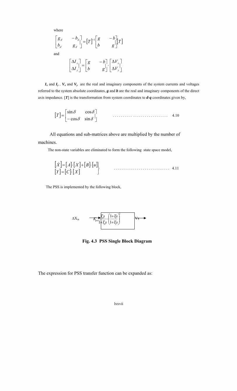
lxxvii

where

[ ] [ ]Tgbbg

Tgb

bg

dd

dd⎥⎦

⎤⎢⎣

⎡ −=⎥

⎦

⎤⎢⎣

⎡ − −1

and

⎥⎦

⎤⎢⎣

⎡∆∆

⋅⎥⎦

⎤⎢⎣

⎡ −=⎥

⎦

⎤⎢⎣

⎡∆∆

y

x

y

x

VV

gbbg

II

Ix and Iy , Vx and Vy are the real and imaginary components of the system currents and voltages

referred to the system absolute coordinates, g and b are the real and imaginary components of the direct

axis impedance. [T] is the transformation from system coordinates to d-q coordinates given by,

[ ] ⎥⎦

⎤⎢⎣

⎡−

=δδδδ

sincoscossin

T . . . . . . . . . . . . . . . . . . . . . . . . . . . . 4.10

All equations and sub-matrices above are multiplied by the number of

machines. The non-state variables are eliminated to form the following state space model,

[ ] [ ] [ ] [ ] [ ][ ] [ ] [ ] ⎭

⎬⎫

⋅=⋅+⋅=

XCYuBXAX&

. . . . . . . . . . . . . . . . . . . . . . . . . . . . . 4.11

The PSS is implemented by the following block,

∆Xin 2

2

1

11

1 ⎟⎟⎠

⎞⎜⎜⎝

⎛++

⋅+ sT

sTsT

sTKpss

ω

ω Vs

Fig. 4.3 PSS Single Block Diagram

The expression for PSS transfer function can be expanded as:

lxxviii

sTsTTsTTTsTT

sTsTK pss ωωωω

⋅+++++

++⋅ 32

22

22

22

2211

)2()2(121

then the block diagram can be separated into three sub-blocks as shown:

V1 Vo

Kpss ∆xin 33

2211

1sTsTsT DDD +++

2211 sTsT NN ++ sTω Vs

Fig. 4.4 System 3-Sub-blocks Diagram

Then,

Kpss ∆xin = V1 + TD1 V2 + TD2V3 +TD3sV3 . . . . . . . . . . . . . . . . . . 4.12

where : sV1 =V2 and sV2 = V3

Hence three new state variables are introduced. Their differential equations are,

inpss

TTT

TT

T

xKVVV

sVsVsV

DD

D

D

D

D

∆⋅⎥⎥⎥

⎦

⎤

⎢⎢⎢

⎣

⎡

+⎥⎥⎥

⎦

⎤

⎢⎢⎢

⎣

⎡⋅

⎥⎥⎥⎥

⎦

⎤

⎢⎢⎢⎢

⎣

⎡

−−−

=⎥⎥⎥

⎦

⎤

⎢⎢⎢

⎣

⎡

33

2

3

1

3

13

2

1

13

2

1

00

100010

. . . . . . . . . 4.13

and the expression for Vo is,

[ ]⎥⎥⎥

⎦

⎤

⎢⎢⎢

⎣

⎡⋅=

3

2

1

211VVV

TTV NNo .. . . . . . . . . . . . . . . . . . . . . . . . . . 4.14

but Vs = s Tω Vo

hence,

lxxix

[ ] [ ] inPSS

T

NN

TT

TT

T

NNs xKTTTVVV

TTTV

DD

D

D

D

D

∆⎥⎥⎥

⎦

⎤

⎢⎢⎢

⎣

⎡

⋅+⎥⎥⎥

⎦

⎤

⎢⎢⎢

⎣

⎡⋅

⎥⎥⎥⎥

⎦

⎤

⎢⎢⎢⎢

⎣

⎡

−−−

⋅= .00

1100010

1

33

2

3

1

3

121

3

2

1

1

21 ωω . . . 4.15

or

inpssD

N

D

DNN

d

DN

D

Ns xK

TTT

VVV

TTT

TTT

TTT

TTT

V ∆⋅⎥⎦

⎤⎢⎣

⎡+⎥⎥⎥

⎦

⎤

⎢⎢⎢

⎣

⎡⋅⎥⎥⎦

⎤

⎢⎢⎣

⎡⎟⎟⎠

⎞⎜⎜⎝

⎛−⎟⎟

⎠

⎞⎜⎜⎝

⎛−−=

3

2

3

2

1

3

221

3

11

3

2 1 ωωω

ω . . . . 4.16

The differential equation representing the generator excitation modified to add the PSS signal Vs

to its input becomes:

( )seefdTfd VKVKEEse

⋅+∆⋅−∆−=∆ 1 . .. . . . . . . . . . . . 4.17

and Vs is substituted from equation 4.16.

The three new state variable equations are added to the state space model and the

input matrix B is redefined (to account for all state variables) as,

⎥⎥⎥⎥⎥⎥⎥⎥⎥⎥⎥⎥

⎦

⎤

⎢⎢⎢⎢⎢⎢⎢⎢⎢⎢⎢⎢

⎣

⎡

⋅

=

3

3

2

10000

0

D

D

N

e

e

T

TTT

TK

B

ω

. . . . . . . . . . . . . . . . . . . . . . . . 4.18

and setting ∆xin = ∆ω then u may be redefined as u = K⋅x, where

[ ]000000 pssKK =

The complete system is now described by

[ ] [ ] [ ] [ ] [ ][ ] [ ] [ ] ⎭

⎬⎫

⋅=⋅+⋅=

XCyXBKXAX&

. . . . . . . . . . . . . . . . . . .. . . . . 4.19

lxxx

(the plus sign indicates that the PSS is positively fed into the AVR circuit)

or

[ ] [ ] [ ][ ] [ ] [ ] ⎭

⎬⎫

⋅=⋅+=

XCYXBKAX&

. . . . . . . . . . . . . . . . . . . . . . . . . 4.20

The damping constant ζ can be found by expressing the mode ( pole ) as

-σ + jωd = -ζωn + j√(1-ζ)2ωn2

therefore ωn and ζ can be found as

ωn = √σ2 + ωd2 , and ζ = -σ/ωn

4.2.2 PSS Design Approaches

4.2.2.1 Calculation of Transfer function Parameters

4.2.2.1.1 Classical Methods

There are several design approaches for decentralized PSSs, given in Yu and Li [25], Gibbard [31],

Lam and Yee [32], Boukarim et-al [33]. Some designs are not robust and are based on one unstable or

lightly damped operating condition, while the other considers a set of cases combined with stochastic

methods. Also investigated are centralized designs where other telemetered signals besides the local

shaft speed are fed into the PSS input. Methods which incorporate Linear Matrix Inequalities to

constrain damping in a well defined area of the left half s-plan have received attention recently[34].

In classical methods, the classical PSS, as given in figure 4.3, is described by the transfer function:

2

2

1

11

1 ⎟⎟⎠

⎞⎜⎜⎝

⎛++

⋅+ sT

sTsT

sTK

w

wPSS

was applied to the input of the AVR of any machine of the multi-machine system. The transfer

function is a lead lag compensator designed to offset the lag effect of the AVR circuit. The values of

the time constant and the gain are determined by trial and error after some experiments. Clearly this is

tedious work and forms the difficult part of the design.

4.2.2.1.2 The New Improved PSS Designed Method

In this study a new, practical and relatively simple approach is proposed which is essentially a

decentralized design involving the shaft speed signal of one generator at a time. The method is based

on curve-fitting of a fixed-parameter lead-lag PSS to drive system poles in the direction of increased

damping using modal sensitivity to a feedback transfer function H(s).

The system is represented by the following block diagram,

lxxxi

Fig 4.5 State Space System with Feedback PSS

The input matrix B relates the output of the PSS to the AVR input of the

concerned machine in the system. The open loop system transfer function G(s) is expressed as

BAsICsusysG 1)()()()( −−== …. . . . . . . . . . . . . .. 4.21

In term of system residues and eigenvalues G(s) can also be expressed as:

∑= −

=n

i i

i

sR

sG1

)(λ

. . . . . . . . . . . . . . . . . 4.22

where Ri is the transfer function residue associated with the mode λi .

Let the PSS transfer function be denoted by k⋅H(s). The closed-loop poles are determined by the roots

of the characteristic equation (for positive feedback)

∑= −

=n

i i

i

ssHkR

1

)(1

λ . . . . . . . . . . . . . . . 4.23

Now if k is sufficiently small then the open loop poles λi ′s are shifted by

)( iii HkR λλ =∆ . . . . . . . . . .. . . . . . . 4.24

( ) ( )( ) ( )sTsT

sTsTK42

31

1111+⋅++⋅+

PSS

C I/s B

A

∆ω u

State-space model of AVR

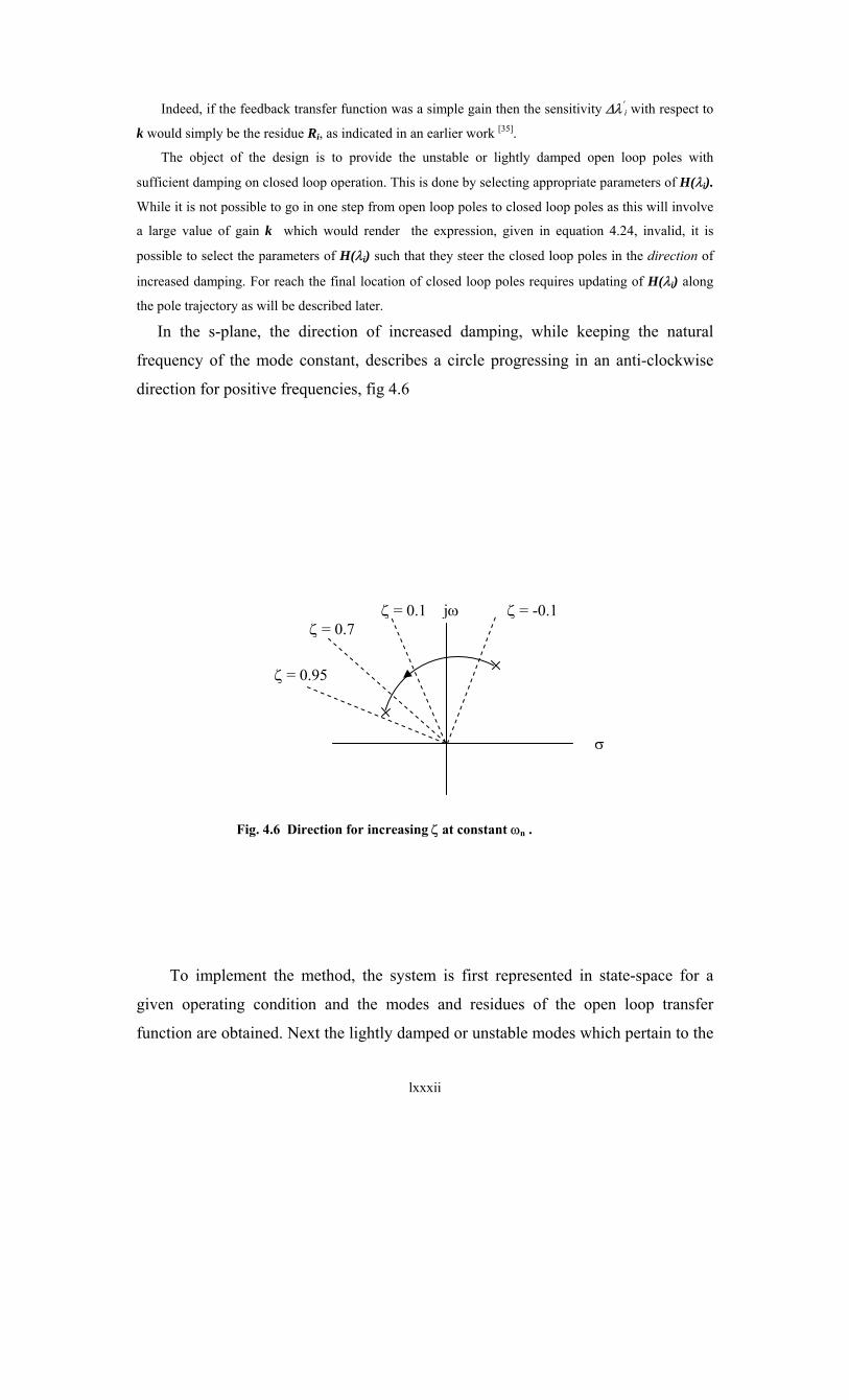
lxxxii

Indeed, if the feedback transfer function was a simple gain then the sensitivity ∆λ′i with respect to

k would simply be the residue Ri, as indicated in an earlier work [35].

The object of the design is to provide the unstable or lightly damped open loop poles with

sufficient damping on closed loop operation. This is done by selecting appropriate parameters of H(λi).

While it is not possible to go in one step from open loop poles to closed loop poles as this will involve

a large value of gain k which would render the expression, given in equation 4.24, invalid, it is

possible to select the parameters of H(λi) such that they steer the closed loop poles in the direction of

increased damping. For reach the final location of closed loop poles requires updating of H(λi) along

the pole trajectory as will be described later.

In the s-plane, the direction of increased damping, while keeping the natural

frequency of the mode constant, describes a circle progressing in an anti-clockwise

direction for positive frequencies, fig 4.6

Fig. 4.6 Direction for increasing ζ at constant ωn .

To implement the method, the system is first represented in state-space for a

given operating condition and the modes and residues of the open loop transfer

function are obtained. Next the lightly damped or unstable modes which pertain to the

σ

jω ζ = -0.1 ζ = 0.1 ζ = 0.7

ζ = 0.95

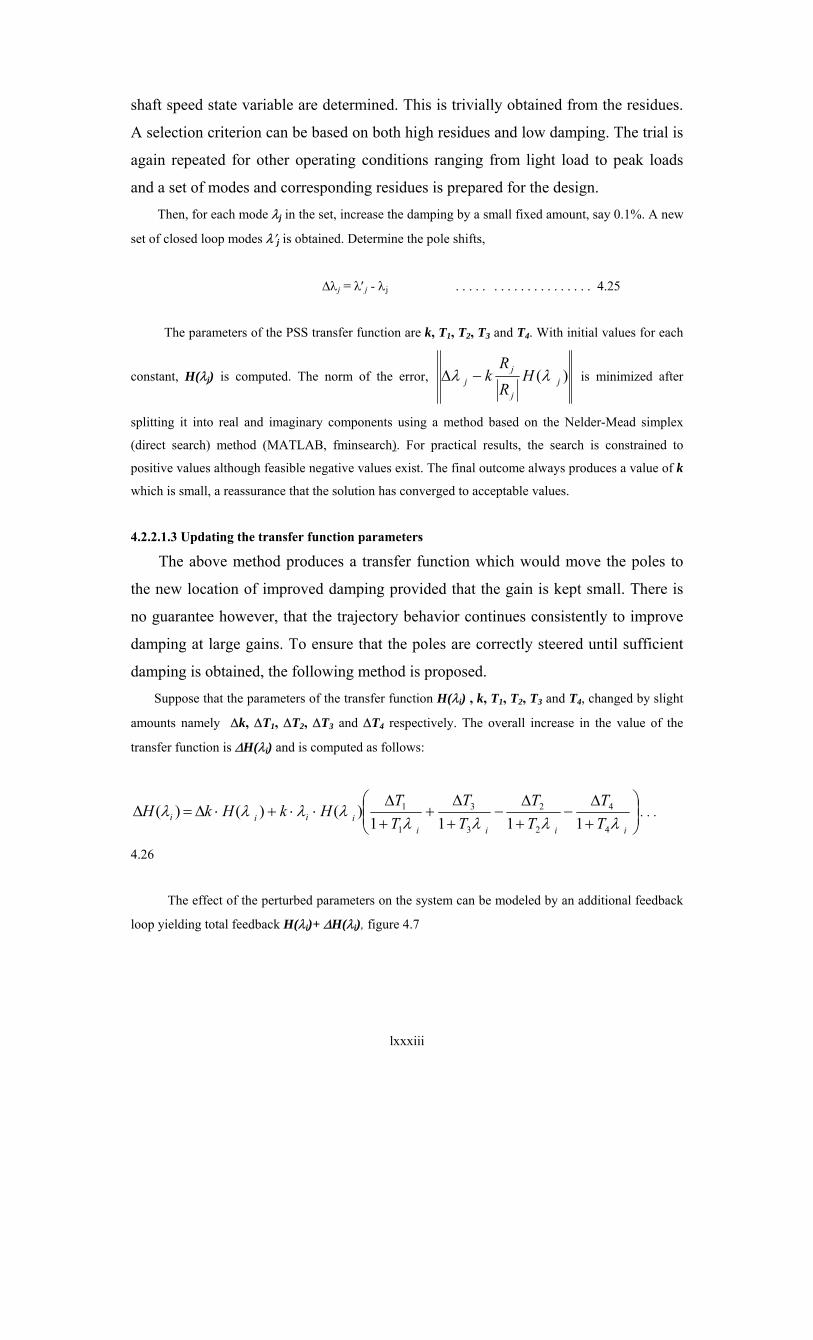
lxxxiii

shaft speed state variable are determined. This is trivially obtained from the residues.

A selection criterion can be based on both high residues and low damping. The trial is

again repeated for other operating conditions ranging from light load to peak loads

and a set of modes and corresponding residues is prepared for the design. Then, for each mode λj in the set, increase the damping by a small fixed amount, say 0.1%. A new

set of closed loop modes λ′j is obtained. Determine the pole shifts,

∆λj = λ′j - λj . . . . . . . . . . . . . . . . . . . . 4.25

The parameters of the PSS transfer function are k, T1, T2, T3 and T4. With initial values for each

constant, H(λj) is computed. The norm of the error, )( jj

jj H

R

Rk λλ −∆ is minimized after

splitting it into real and imaginary components using a method based on the Nelder-Mead simplex

(direct search) method (MATLAB, fminsearch). For practical results, the search is constrained to

positive values although feasible negative values exist. The final outcome always produces a value of k

which is small, a reassurance that the solution has converged to acceptable values.

4.2.2.1.3 Updating the transfer function parameters

The above method produces a transfer function which would move the poles to

the new location of improved damping provided that the gain is kept small. There is

no guarantee however, that the trajectory behavior continues consistently to improve

damping at large gains. To ensure that the poles are correctly steered until sufficient

damping is obtained, the following method is proposed. Suppose that the parameters of the transfer function H(λi) , k, T1, T2, T3 and T4, changed by slight

amounts namely ∆k, ∆T1, ∆T2, ∆T3 and ∆T4 respectively. The overall increase in the value of the

transfer function is ∆H(λi) and is computed as follows:

⎟⎟⎠

⎞⎜⎜⎝

⎛+∆

−+∆

−+∆

++∆

⋅⋅+⋅∆=∆iiii

iiii TT

TT

TT

TT

HkHkH 4

4

2

2

3

3

1

1 1111

)()()(λλλλ

λλλλ . . .

4.26

The effect of the perturbed parameters on the system can be modeled by an additional feedback

loop yielding total feedback H(λi)+ ∆H(λi), figure 4.7

lxxxiv

Fig. 4.7 Additional Feedback to the System

The feedback loop involving the PSS transfer function H(s) can be incorporated into the state-space

model to arrive at a new state space matrices Ad, Bd and Cd . The feedback loop now only involves

∆H(s). As before residues are calculated and used in the expression,

)( iii HR λλ ∆=∆ . . . . . . . . . . . . . 4.27

A significant difference is that ∆H(s) does not have to be multiplied by a small gain k because it is

itself sufficiently small to preserve the accuracy of the expression.

To implement, first incorporate the PSS model into the system as follows:

1. Set iteration count to1.

2. Improve the modes slightly by setting the gain at a low value, say 0.1 or less.

Due attention should be taken to ensure that the gain is small at all modal

frequencies concerned, not only the steady state gain. 3. Obtain a set of open loop (as far as ∆H(s) is concerned) modes and residues for this gain for the

required range of operating conditions. After application of the PSS participation of the state

variables to the modes may change, so ensure that the proper modes are selected.

C I/s B

A

∆ω u

State-space model of AVR

H(s)

∆H(s)

lxxxv

4. Next, improve the damping of the new modes slightly (0.1%) to get new modes.

5. As before compute the mode shift ∆λj

6. Minimize )( jj

jj H

R

Rk λλ −∆ after initializing values for ∆k, ∆T1, ∆T2, ∆T3 and ∆T4 ; a

reasonable start is 0 for all parameters.

7. Update T1, T2, T3 and T4 . It is not necessary to update k since the gain is controlled at each

step.

8. Increase the gain by 0.1 (or less), advance iteration count and repeat until sufficient damping is

obtained.

Note that the emphasis of the design lies in guiding the poles through the direction of maximum

damping. It is difficult for the feedback transfer function to shift all poles equally since the shifts are

related to the transfer function by residues of different magnitudes and directions. Convergence to a

solution can be aided by stripping each mode shift of its residue magnitude sensitivity and retaining

only orientation sensitivity. This is done by dividing each residue by its magnitude. The norm of the

error hence takes the form )( jj

jj H

R

Rk λλ −∆ . While a reasonable solution emerges both without

and with residue scaling, the latter method usually yields faster convergence.

4.3 Implementation of The Classical and The New Designed PSS

4.3.1 Implementation of The Classical PSS

The classical PSS described above was applied to the input of the AVR of

machine 1 in the 9-bus system figure 2.6. The constants were chosen (by trial and

error) as follows: KPSS = 10, TW = 5 , T1 = 0.5 and T2 = 0.03. The transfer function

becomes,

2

03.015.01

51510 ⎟

⎠⎞

⎜⎝⎛++

⋅+

⋅ss

ss

This transfer function is a lead lag compensator designed to offset the lag effect of

the AVR circuit. The bode plot of the PSS is shown in fig. 4.8.

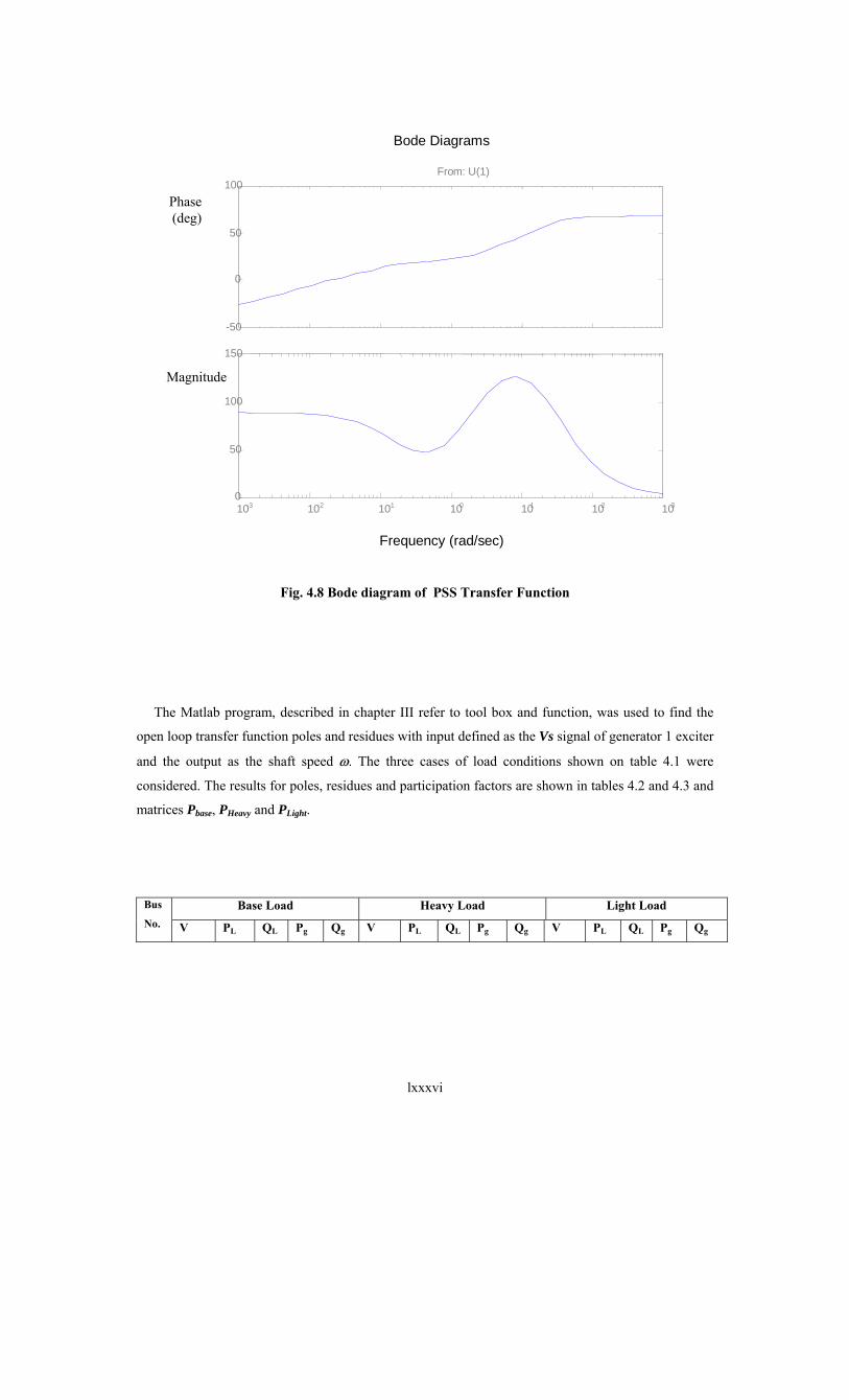
lxxxvi

Frequency (rad/sec)

Bode Diagrams

-50

0

50

100From: U(1)

10-3 10-2 10-1 100 101 102 1030

50

100

150

Fig. 4.8 Bode diagram of PSS Transfer Function

The Matlab program, described in chapter III refer to tool box and function, was used to find the

open loop transfer function poles and residues with input defined as the Vs signal of generator 1 exciter

and the output as the shaft speed ω. The three cases of load conditions shown on table 4.1 were

considered. The results for poles, residues and participation factors are shown in tables 4.2 and 4.3 and

matrices Pbase, PHeavy and PLight.

Base Load Heavy Load Light Load Bus

No. V PL QL Pg Qg V PL QL Pg Qg V PL QL Pg Qg

Phase (deg)

Magnitude

lxxxvii

1 2 3 4 5 6 7 8 9

1.025 1.025 1.04 1.026 0.996 1.013 1.026 1.016 1.032

0.0 0.0 0.0 0.0 1.25 0.9 0.0 1.0 0.0

0.0 0.0 0.0 0.0 0.5 0.3 0.0 .35 0.0

1.63 0.85 0.0 0.0 0.0 0.0 0.0 0.0 0.0

.07 -.11 0.0 0.0 0.0 0.0 0.0 0.0 0.0

1.025 1.025 1.04 0.993 0.930 0.962 0.996 0.967 1.009

0.0 0.0 0.0 0.0 1.25 0.9 0.0 1.0 0.0

0.0 0.0 0.0 0.0 1.0 0.6 0.0 0.8 0.0

1.63 0.85 0.0 0.0 0.0 0.0 0.0 0.0 0.0

.563

.308 0.0 0.0 0.0 0.0 0.0 0.0 0.0

1.025 1.025 1.04 1.055 1.055 1.06 1.049 1.052 1.05

0.0 0.0 0.0 0.0 0.4 0.3 0.0 0.3 0.0

0.0 0.0 0.0 0.0 .15 0.1 0.0 0.1 0.0

0.5 -.38 0.0 0.0 0.0 0.0 0.0 0.0 0.0

0.3 -.43 0.0 0.0 0.0 0.0 0.0 0.0 0.0

Fig. 4.1 Three Cases of Load Conditions

Note that the angles for generator voltages as follows: For base load δ1 = 9.3° , δ2 = 4.7°

For heavy load δ1 = 9.7° , δ2 = 4.7° For light load δ1 = 3° , δ2 = 1.9°

Frequency Modes

Base Load Heavy Load Light Load

Mode 1 Mode 2 Mode 3 Mode 4

-0.2953 ± 11.7403i -0.2216 ± 7.9514i -1.0088 ± 1.8533i -1.0779 ± 0.9563i

-0.2353 ±11.4396i -0.2439 ± 9.7778i -1.1234 ± 1.3488i -1.1649 ± 1.1817i

-0.2122 +12.1308i -0.2247 + 9.8960i -1.1426 + 1.4938i -1.1880 + 1.3310i

Table 4.2 Open-Loop Poles for the Three

Cases of Load Conditions

Residues Frequency

Modes Base Load Heavy Load Light Load

Mode 1 Mode 2 Mode 3 Mode 4

0.0017 ± 0.0003i 0.0131 ± 0.0031i -0.0117 ± 0.0072i -0.0031 ± 0.0035i

0.0000 ± 0.0000i 0.0117 ± 0.0025i -0.0117 ± 0.0103i 0.0000 ± 0.0000i

0.0000 + 0.0000i 0.0113 + 0.0024i -0.0113 + 0.0092i 0.0000 + 0.0000i

Table 4.3 Open-Loop Residues for the Three

lxxxviii

Cases of Load Conditions The calculated participation factors are: Mode 1 Mode 2 Mode 3 Mode 4

E′q1 0.00 0.00 0.03 0.03 0.42 0.42 0.18 0.18 E′q2 0.02 0.02 0.00 0.00 0.15 0.15 0.51 0.51 Efd1 0.00 0.00 0.01 0.01 0.41 0.41 0.18 0.18

Pbase = Efd2 0.00 0.00 0.00 0.00 0.15 0.15 0.50 0.50 ω1 0.07 0.07 0.43 0.43 0.01 0.01 0.00 0.00 ω2 0.43 0.43 0.07 0.07 0.00 0.00 0.01 0.01 δ1 0.07 0.07 0.43 0.43 0.01 0.01 0.00 0.00 δ2 0.43 0.43 0.07 0.07 0.00 0.00 0.01 0.01

Mode 1 Mode 2 Mode 3 Mode 4

E′q1 0.0257 0.0257 0.5968 0.5968 0.0000 0.0000 0.0000 0.0000 E′q2 0.0000 0.0000 0.0000 0.0000 0.0210 0.0210 0.6117 0.6117 Efd1 0.0035 0.0035 0.5872 0.5872 0.0000 0.0000 0.0000 0.0000

PHeavy = Efd2 0.0000 0.0000 0.0000 0.0000 0.0033 0.0033 0.6031 0.6031 ω1 0.4978 0.4978 0.0084 0.0084 0.0000 0.0000 0.0000 0.0000 ω2 0.0000 0.0000 0.0000 0.0000 0.4977 0.4977 0.0072 0.0072 δ1 0.4978 0.4978 0.0084 0.0084 0.0000 0.0000 0.0000 0.0000 δ2 0.0000 0.0000 0.0000 0.0000 0.4977 0.4977 0.0072 0.0072

Mode 1 Mode Mode 3 Mode 4 E′q1 0.0234 0.0234 0.5788 0.5788 0.0000 0.0000 0.0000 0.0000 E′q2 0.0000 0.0000 0.0000 0.0000 0.0178 0.0178 0.5865 0.5865 Efd1 0.0017 0.0017 0.5717 0.5717 0.0000 0.0000 0.0000 0.0000

PLight = Efd2 0.0000 0.0000 0.0000 0.0000 0.0017 0.0017 0.5811 0.5811 ω1 0.4996 0.4996 0.0061 0.0061 0.0000 0.0000 0.0000 0.0000 ω2 0.0000 0.0000 0.0000 0.0000 0.4991 0.4991 0.0045 0.0045 δ1 0.4996 0.4996 0.0061 0.0061 0.0000 0.0000 0.0000 0.0000 δ2 0.0000 0.0000 0.0000 0.0000 0.4991 0.4991 0.0045 0.0045

Mechanical modes of generator 1 (mode2)

Mechanical modes of generator 1 (mode2)

Mechanical modes of generator 1 (mode2)

lxxxix

From the results of the base load, the modes of interest are the lightly damped mechanical modes

with poles at -0.2953 ± j11.7403 and -0.2216 ± j7.9514. The participation matrix shows that the first

mode is closely associated with ω and δ of generator2 (ω2 and δ2), while the second mode is associated

with the same states of generator1 (ω1 and δ1). The bode diagram of fig. 4.8 shows that the PSS

provides phase lead action in this range.

Application of the PSS on generator 1 with a gain Kpss equal to 10 provides good damping of

mode 2 and moderate improvement for mode 1. Table 4.4 below shows damping ratios of all the modes

expressed in percent before and after application of PSS.

Mode ζ (%) Without PSS on machine 1

ζ (%)With PSS on machine 1

mode1 2.5 6.7 mode2 2.8 26.9 mode3 47.8 44.4 mode4 74.8 74.4

Table 4.4 Damping Ratios for 9-bus System Modes

A damping ratio of 10% or more is considered sufficient. Clearly the PSS provides adequate

damping for mode 2. Mode 1 is also notably improved while the non-mechanical modes remain

unchanged. The same procedure could be done for machine 2, with different setting for transfer

function constants. Comparing the results of installation the PSS on generator 1 and generator 2, the

suitable location for good damping can be selected.

4.3.2 Classical Method Robustness

A major concern in PSS design is that it provides good damping at all operating loads, ranging

from heavy generator loading to islanding conditions. A design that satisfies this criterion is known as a

robust design. Difficulties in achieving robust control lead some utilities to consider adaptive PSS

design as opposed to fixed parameter control. A fixed parameter approach is attractive, however,

because of its simplicity.

To test the PSS described above for robustness, the three cases of loading conditions, given on table

4.1 for the 9-bus system were investigated;

1. The base load case.

2. A heavy loading condition.

3. A light loading condition.

xc

A load flow was carried out for each case to determine the steady state operating conditions. All

PSS parameters were fixed, including the gain. The following table 4.5 shows the damping obtained for

all three conditions.

Mode ζ (%) Without PSS on machine 1

ζ (%)With PSS Case 1

ζ (%)With PSS Case 2

ζ (%)With PSS Case3

mode1 2.5 6.7 7.0 2.4

mode2 2.8 26.9 29.2 28.2

mode3 47.8 44.4 40.5 40.7

mode4 74.8 74.4 60.7 82.8

Table 4.5 The Results for Robustness Tests

Indications are that, as far as mode 2 is concerned, the design is robust and the PSS is capable of

injecting sufficient damping over a wide range of operating conditions.

4.3.3 Implementation of the New Designed Method

Using the previous example of the 9-busbar system and from the results of the base load condition

case, it is clear that the lightly damped mechanical mode associated with generator1 (ω1 and δ1) is

mode 2;

-0.2216 + j7.9514 and -0.2216 - j7.9514

with corresponding residues

0.0131 + j0.0031 and 0.0131 - j0.0031

The study is repeated for heavy load and light load cases shown on table 4.2 yielding the following

results for mode 2:

Heavy Load

Modes: -0.2016+7.3710i -0.2016-7.3710i

Residues: 0.0147+0.0042i 0.0147+0.0042i

Light Load

Modes: -0.0919+6.0947i -0.0919-6.0947i

xci

Residues: 0.0100+0.0043i 0.0100-0.0043i

Next, A MATLAB program written according to the algorithm given in section 4.2.2.2 was used.

Which substitutes initial values of k, T1, T2, T3 and T4 into the feedback (PSS) transfer function H(λj)

for each mode λj. The norm of the error ⎢⎢ )( jjj HkR λλ −∆ ⎢⎢ is minimized to obtain a local

minima for values of T1, T2, T3 and T4. It must be emphasized that many local minimum exist and

hence the minimization process is sensitive to the initial choice of parameters. A good idea is to

experiment with different starting values and to select an outcome with the lowest error.

In this particular case an outcome which takes into account all modes and residues above is:

T1 = 1.035 T2 = 0.0 T3 = 0.706 T4 = 0.0 k = 0.0013

The initial design is then substituted in another sub-program, written within the main program,

which updates the values of T1, T2, T3 and T4 to improve the damping according to the algorithm

outlined previously. A particular weighting factor is based on finding the damping ratio for each mode

Dj and then selecting the maximum damping for all modes, Dmax. Each mode shift is then

weighted by (Dmax/Dj)m which favors the weaker modes with larger shifts. The exponent m is

selected experimentally in the range 1–2.

The program displays the results of the improved damping ratio (ζ) and the gain (k) in each

iteration, so, it is easy to stop the program when the desired improvement is obtained associated with a

suitable value for gain. Table 4.6 show the progress of the improving damping factors and

corresponding gains.

Damping Factors (ζ ) Gain

k Mode1 Mode2 Mode3 Mode4 0.1500 0.4000 0.6500 0.9000 1.1500 1.4000 1.6500 1.9000 2.1500 2.4000 2.6500 2.9000 3.1500 3.4000 3.6500 3.9000 4.1500 4.2000 4.2500 4.3000

0.0398 0.0398 0.0347 0.0347 0.0223 0.0223 0.0348 0.0348 0.0597 0.0597 0.0544 0.0544 0.0351 0.0351 0.0539 0.0539 0.0799 0.0799 0.0742 0.0742 0.0480 0.0480 0.0732 0.0732 0.0962 0.0962 0.0907 0.0907 0.0600 0.0600 0.0888 0.0888 0.1120 0.1120 0.1065 0.1065 0.0717 0.0717 0.1039 0.1039 0.1283 0.1283 0.1229 0.1229 0.0841 0.0841 0.1196 0.1196 0.1441 0.1441 0.1392 0.1392 0.0966 0.0966 0.1353 0.1353 0.1602 0.1602 0.1561 0.1561 0.1097 0.1097 0.1517 0.1517 0.1761 0.1761 0.1732 0.1732 0.1232 0.1232 0.1684 0.1684 0.1902 0.1902 0.1889 0.1889 0.1358 0.1358 0.1841 0.1841 0.2035 0.2035 0.2045 0.2045 0.1485 0.1485 0.2000 0.2000 0.2161 0.2161 0.2200 0.2200 0.1616 0.1616 0.2162 0.2162 0.2279 0.2279 0.2356 0.2356 0.1748 0.1748 0.2327 0.2327 0.2385 0.2385 0.2507 0.2507 0.1880 0.1880 0.2489 0.2489 0.2482 0.2482 0.2654 0.2654 0.2011 0.2011 0.2648 0.2648 0.2579 0.2579 0.2795 0.2795 0.2143 0.2143 0.2799 0.2799 0.2697 0.2697 0.2964 0.2964 0.2273 0.2273 0.2942 0.2942 0.2724 0.2724 0.2971 0.2971 0.2299 0.2299 0.2969 0.2969 0.2754 0.2754 0.2998 0.2998 0.2325 0.2325 0.2996 0.2996 0.2784 0.2784 0.3373 0.3373 0.2754 0.2754 0.2998 0.2998

xcii

Table 4.6 Progress of Improving Damping Factors

The final suitable outcome of the gain and time constants are:

k = 4.3

T1 = 1.19

T2 = 0.00001

T3 = 0.668

T4 = 0.056

The corresponding bode plot of the new designed PSS is shown in figure 4.9

Fig. 4.9 Bode plot of the New method Designed

Frequency (rad/sec)

Bode Diagrams

0

50

100

150

10-2

10-1

100

101

102

103

104

0

50

100

150

Phase (deg)

Magnitude

xciii

Clearly, this results would yield damping ratios between 0.23 and 0.29 for mode 2

for all load cases. The design is robust and yields good damping. It may be remarked

that slightly better results were achieved through the classical method of trial and

error described earlier. However, trial and error is completely arbitrary and offers no

insight into the design and cannot be relied on to achieve good results in all cases.

Chapter V Improving The Stability Using

Controlled Series Compensation 5.1 Introduction

The controlled series compensation, (CSC) can be used to control and increase

the damping of poorly damped power system dynamic oscillation modes in a multi

machine system. The CSCs have the ability to change their reactances, either continously or step-wise, by controlling

the firing angle of thyristors[37,38,39,40] although research on how to control these devices to improve the

stability of power systems is still at a preliminary stage.

In practical power systems the effective performance of a CSC control scheme requires that the

CSC be located at an optimum point in the network[41] . Also for a certain power system a single CSC

may not be able to damp out effectively all the significant oscillation modes. In such a situation

coordinated operation of several CSCs installed at different locations in the network may be required to

achieve a significant improvement in the power system stability margin. Available experience, either

on selecting the most effective location of CSC or on coordinating controllers is still at early stages,

although some efforts have been attempted [41] .

In the following sections a description of a design procedure for CSC controllers to increase the

damping of all poorly damped oscillation modes is given, with illustrated example using state

variables.

5.2 System Modelling and Eigenvalues

If the effect of damper windings, stator transients and rotor winding resistance are

ignored, then each synchronous machine and its excitation system can be modelled

xciv

using the set of the previous non-linear dynamic equations 3.90-3.93 which can be

written again as,

[ ]dddqfddo

q iXXeeTdt

de⋅−−−= )(1 ''

'

'

. . . . . . . . . . . . . 5.1

[ ]fdttrefe

fd ekVVTdt

de−⋅−= )(1

. . . . . . . . . . . . . 5.2

[ ]em PPHdt

dw−=

21

. . . . . . . . . . . . . . . . . . . . . 5.3

sdtd ωωδ

⋅−= )1( . . . . . . . . . . . . . . . . . . . . . . . . 5.4

where

maxmin

''

22

fdfdfd

ddqq

qqd

qqdde

qdt

eee

iXev

iXv

ivivP

vvv

≤≤

−=

=

+=

+=

For each CSC in the system the relationship between the controlled reactance and

the input to CSC controller can be described by the following equation,

( ) maxmin ,1llll

x

l xxxxuTdt

dx≤≤−= . . . . . . .. . . . . . . . . 5.5

where u is the control signal

Tx is the time constant of the CSC

xlmin and xlmax are the control limits of the CSC

Equation 5.5 is considered as the fifth state equation for the power system described by equations

5.1-5.4.

For a multi-machine power system with N-buses and m synchronous machines the network nodal

current injection equation is given by

I = YV . . . . . . . . . . . . . . . . . . . . . . . . . . . . . . . . . . 3.95

where I = [I1, I2, . . . . . .,Im, 0, . . . .,0]T

V= [V1,V2, . . . . ,Vm, . . . . .,Vn]T

and Y is the N x N admittance matrix which is a function of the reactances of the CSCs, xli; i = 1,2, .

. . ,l in the system, l is the number of the CSCs.

xcv

Using the equations 5.1 – 5.6, the system with l-CSCs can be represented by a set of non-linear

state equation of the form,

),( uxfx =& . . . . . . . . . . . . . . . . . . . . . . . . . . . . 5.6

where [ ]Tlllmmfdmfd'qm

'q , . . ,x,x, . . . ,δ,δ, . . . ,ω,ω, . . ,e,ee,. . . . ,ex 11111= and

[ ]Tl,u, . . . . uu 1=

f represent vectors of nonlinear functions formed by combining equation 5.1–5.6 for all

synchronous machines and CSCs in the system.

The non-linear equation 5.7 can be linearized around the system operating point for small changes

of the state vector X and the control input U, by the state equation,

UBXAX ∆+∆=∆•

. . . . . . . . . . . . . . . . . . . . . . . 5.7

5.3 Algorithm to Find ∆X

Using two virtual axes y and x the following equation which describes the relations

between the machines and system parameters can be defined as,

⎪⎪⎪⎪⎪⎪⎪⎪⎪⎪

⎭

⎪⎪⎪⎪⎪⎪⎪⎪⎪⎪

⎬

⎫

=+=

−=

+=

−=⎥⎥⎦

⎤

⎢⎢⎣

⎡

−

+=

+=

−=

=

=

∑

∑

=

=

, . . . ,mfor ivvv

vvv

iii

iii

xivxiv

a

gvbvi

bvgvi

vv

vv

iyixq

iyixd

iyixq

iyixd

qyx

qxyi

n

jijyjijxjy

n

jijyjijxjx

iiy

iix

iii

iii

iii

iii

iii

iii

i

i

i

i

1sincos

cossin

sincos

cossin

tan

sin

cos

1

1

δδ

δδ

δδ

δδ

δ

δ

δ

. . . . . . . . . . . . 3.98

The over-all state matrix A can be found by linearization equations 5.1 –5. 5 and 5.9 around the

operating point as follows,

( ) dddqTTq ixxeqedodo

∆−−∆−=∆ 11& . . . . . . . . . . . . . . . . . . . 5.8

xcvi

( ) dddqTqTf ixxeedodo

∆−−∆−=∆ 11& . . . . . . . . . . . . . . . . . . . 5.9

fdTeT evKee∆−∆−=∆ 11ω& . . . . . . . . . . . . . . . . . . . 5.10

ωωδ ∆=∆ && . . . . . . . . . . . . . . . . . . . 5.11

xx

ll T

UTx

x ∆+

∆−=∆& . . . . . . . . . . . . . . . . . . 5.12

δδδ ∆+∆−∆−∆−= qyxd iiii cossin0 . . . . . . . . . . . . . . . . . . 5.13

δδδ ∆−∆+∆−∆−= qyxq iiii sincos0 . . . . . . . . . . . . . . . . . . . 5.14

qqd ixv ∆+∆−=0 . . . . . . . . . . . . . . . . . . 5.15

dddqq ixev ∆−∆+∆−=0 . . . . . . . . . . . . . . . . . . 5.16

yxx vbvgi ∆−∆+∆−=0 . . . . . . . . . . . . . . . . . . 5.17

yxy vgvbi ∆+∆+∆−=0 . . . . . . . . . . . . . . . . . . 5.18

where b and g are the real and imaginary parts of system admittance Y, for the lines without

installed CSC.

δδδ ∆+∆+∆+∆−= yqdx vvvv cossin0 . . . . . . . . . . . . . . . . . . 5.19

δδδ ∆+∆+∆−∆−= xqdy vvvv sincos0 . . . .. . . . . . . . . . . . . . 5.20

qvv

dvv vvv qd ∆+∆+∆−=0 . . . . . .. . . . . . . . . .. . 5.21

When CSC is installed in any line, equations 5.17 and 5.18 will be variable of series compensator

Xl, the new injected current equations for the lines with installed CSC could be written as;

ylxx vxbgvi )( +−= . . . . . . . . . . . . . . . . . . . . . . . . . . . 5.24

xlyy vxbbvi )( ++= . . . . . . . . . . . . . . . . . . . . . . . . . . . 5.25

which can be linearized as;

lyyxx xvvbvgi ∆−∆−∆=∆ . . . . . . . . . . . . . . . .. . . . . . . 5.26

lxxyy xvvbvgi ∆+∆+∆=∆ . . . . . . . . . . . . . . .. . . . . . . . 5.27

The admittance matrix y is a function of state variable xl1, . . .,xlm so it is difficult to linearize a

multi-machine system with installed CSCs.[42,43] .

A new simple approach to solve this problem can be described as follows:

xcvii

Write the over-all state matrix for the system using equation 5.10-5.27 without reducing the

admittance matrix Y to the number of generator buses , so that it contains the actual reactances of the

lines.

Insert the CSC in the desired line. Note that, this insertion will change the coefficients of ∆xl , ∆vx

and ∆vy for this line only.

Reduce the obtained over all matrix to the number of state variable, n, then the state matrix A will

be of order n x n . Notice that n = 4m+l. (m = number of machine, l = number of CSC equql 1 for one

CSC)

The final state matrix A and matrix B of the controll signal can be written as,

⎪⎪⎪⎪⎪⎪⎪⎪⎪

⎭

⎪⎪⎪⎪⎪⎪⎪⎪⎪

⎬

⎫

⎥⎥⎥⎥⎥⎥⎥⎥

⎦

⎤

⎢⎢⎢⎢⎢⎢⎢⎢

⎣

⎡

=

⎥⎥⎥⎥⎥⎥

⎦

⎤

⎢⎢⎢⎢⎢⎢

⎣

⎡

=

xT

nnn

n

n

B

and

aa

aaaaaa

A

1

2n1

22221

11211

.

.00

.....a.

. ...............

. . . . . . . . . . . . . . . . . . .. 5.28

From the participation matrix given by equation 3.45, it can be shown that the last row and column

of state matrix A, are the only row and column which depend on the location of the CSC. To prove

this, the controllbility of the participation matrix can be invoked as follows

bb ⋅=′ φ . . . . . . . . . . . . . . . . . . . . . . . . . . . . . . . . 5.29

Which show that all elements are zeros, except those on the last row.

5.4 Design of CSC Controllers for Multimachine Systems 5.4.1 Pole Placement Technique

The open-loop poles of the system described by equation 5.8 are the eigen values of the matrix A.

Assume that the state feedback controller defined by the following equation,

XKU gain∆−=∆ . . . . . . . . . . . . . . . . . . . . . . . . . . . . 5.30

xcviii

is used, then the closed-loop system can be described by,

XBKAX gain ∆−=∆•

)( . . . . . . . . . . . . . .. . . . . . . . . . . . . 5.31

where Kgain is the feedback gain matrix given by,

⎥⎥⎥⎥⎥

⎦

⎤

⎢⎢⎢⎢⎢

⎣

⎡

=

+

+

141

14111

ml,l,

m,,

gain

.,k . . . . .k .. ..

,k . . . . .k

K . . . . . . . . . . . . . . . . . . . 5.32

The poles of this feed back system are the eigenvalues of the matrix [A-BKgain].

By assigning the desired close–loop poles, the feedback gains Kgain for the controllers

can be determined.

Theoretically, the further the poles are shifted to the left –hand side, away from

the imaginary axis, the better the damping of the oscillation, but a larger shift also

requires a larger controller action. In practice each controller has a finite capacity and

if the required control action goes beyond these limits the desired damping effect of

the controller will be diminished, or even become negative[41] , therefore, the selection

of the close –loop pole positions must be realistic.

5.4.2 Determination of the most effective location for a CSC

To identify the location for the CSC is the most important aspect of designing a

CSC controller for a multi-machine power system. A proper location for the CSC

may lead to overall improvement of the damping factors for all the poor dynamic

modes.

For a system with n-dynamic modes, the Laplace transform of any selected output

variable y(s) can be shown to be related to the Laplace transform of the input U(s) by,

)()(1

1 sus

Rs

Rsy

n

n⎟⎟⎠

⎞⎜⎜⎝

⎛−

+⋅⋅+−

=λλ

. . . . . . . . . . . . . . . . . . . 5.33

where λ1, . . . . . ,λn are the eigenvalues of the system and the R1, . . ,Rn are the

corresponding residues. The impulse response of the output y(t) is given by,

xcix

∑=

−=n

i

tieRty

1)( λ . . . . . . . . . . . . . . . . . . . . . . . . . . . . . 5.34

The impulse response associated with any complex conjugate eigenvalue

pair, a ± jb can be further simplified to take the form,

222 )sin(2)( αα ++= btqpety t . . . . . . . . . . . . . . . . . . . . 5.35

where p ± jq is the corresponding residue pair and )(tan 1qp−=α .

The degree of controllability of a given mode in the output y(t) through the control

input u(t) is indicated by the magnitude of the corresponding residue )( 22 qp + .The

most effective location for a CSC is that where the controller can exercise a sufficient

degree of controllability over all the required oscillation modes through its control

input. Therefore by analyzing the residue associated with the power angle oscillations

for different controller locations the best location for the controller can be obtained.

5.5 Description of CSC Digital Programme For Dynamic Stability

The program for investigation of the effect of the CSC on the dynamic stability

was written using MATLAB 5.1 . The programme consists of three main parts. The

first part is for determination the elements of state matrix A, when a CSC is installed

in any line. The second part is to determine the eigenvalues of the state matrix; and

the third part is to determine the participation matrix before and after shifting the

poles to the negative left side.

In order to test the programme, the simple nine busbar system given in chapter

three was taken as an example, the required data in addition to the data given in

chapter three is given in table 5.1. The reactance values are in p.u. on 100 MVA base.

The time constant Tx of the CSC is assumed to be 0.5 and the capacity of the CSC is

assumed to be ±0.08 p.u.

The resultant state matrices A and B are given by ,

-0.5560 0.1137 0.1695 0.0000 0.0000 0.0000 -0.3560 0.0950 a19

0.1824 -0.6513 0.0000 0.1698 0.0000 0.0000 0.1409 -0.4204 a29

c

-24.4080 -7.2461 -2.0000 0.0000 0.0000 0.0000 -1.9971 -1.4011 a39

-7.5317 -22.0355 0.0000 -2.0000 0.0000 0.0000 1.7813 -6.3765 a49

A = -0.2497 0.0306 0.0000 0.0000 0.0000 0.0000 -0.1951 0.0443 a59

0.0960 -0.4013 0.0000 0.0000 0.0000 0.0000 0.1103 -0.3343 a69

0.0000 0.0000 0.0000 0.0000 377.1429 0.0000 0.0000 0.0000 0.0

0.0000 0.0000 0.0000 0.0000 0.0000 377.1429 0.0000 0.0000 0.0

0.0000 0.0000 0.0000 0.0000 0.0000 0.0000 0.0000 0.0000 -2

⎥⎥⎥⎥⎥⎥⎥⎥⎥⎥⎥⎥

⎦

⎤

⎢⎢⎢⎢⎢⎢⎢⎢⎢⎢⎢⎢

⎣

⎡

=

0.200.000.000.000.000.000.000.000.0

B

The elements a19 – a69 of matrix A depend on the location of the CSC. Taking

the three longest transmission lines in this system, ” line 5-7, line 3-6 and line 3-8”,

for possible CSC locations, then the elements a19 – a69 of matrix A were found to be

as in table 5.2.

The open-loop poles of this system is independent of the location of the CSC

controller and are given in table 5.3. The pole position , from this table, show that the

natural damping of the oscillation modes, mode 1 and mode 2, with associated

frequencies 11.7427 and 7.9529 rad/s, respectively, is very low. The damping

associated with these two modes can be improved by placing the closed-loop poles at

new positions by moving them slightly ( -1 ) to the negative left side. This is shown in

table 5.3. No attempt is made to control the other modes, which already lies far on the

negative left side, i.e. have sufficient damping.

The feed back control gains obtained for the closed loop is shown on table 5.4.

To select the most effective location for CSCs, the residues for different oscillation

modes must be found. The output of the system when determining the residues is

considered to be the power angle of machine 1 and that of machine 2, respectively.

ci

Since the control objective is to damp modes 1 and 2, only the controllability of these

two oscillation modes needs to be considered. The residues in table 5.5 show that

when a CSC is installed in line 5-7, the residues for mode 1 are much smaller than

that of CSCs at other positions, whereas when a CSC is installed in line 3-8 the

residue for mode 1 and mode 2 is much smaller. Only when a CSC is installed in line

3-6 do the residues for both modes have reasonable values. These observation imply

that:

1. If only one CSC is to be installed then, of the three locations analyzed, the

most effective location for installing a CSC device is on transmission line

3-6.

2. Good damping may also be obtained by coordinated use of CSC devices

on lines 5-7 and 3-8, with the CSC on line 5-7 for damping mode 2 and on

line 3-8 for damping mode 1.

Parameters Generator 1 Generator2

Xd (p.u.) X’

d (p.u.) Xq (p.u.) T’

do (s) H (MWs/MVA) ke Te (s) Efd min (p.u.) Efd max (p.u.)

0.8958 0.1198 0.8645 5.9 6.4 25.0 0.5 -4.0 4.0

1.3125 0.1813 1.2578 5.89 3.01 25.0 0.5 -4.0 4.0

Table 5.1

Generator and Excitation Data for the 9-busbar System

CSC location a19 A29 a39 a49 a59 a69

Line 5-7

Line 3-6

Line 3-8

0.037

0.003

0.019

0.031

0.084

0.098

-18.055

-12.087

-17.724

-12.598

-20.365

-23.818

-0.053

-0.047

-0.061

-0.037

-0.037

-0.043

Table 5.2

Variation of the elements of matrix A with CSC location

cii

Oscillation modes Open-loop poles Closed-loop poles

Mode 1

Mode 2

Mode 3

Mode 4

Mode 5

-0.2953 ±11.7427i

-0.2216 ± 7.9529i

-1.0088 ± 1.8533i

-1.0779 ± 0.9563i

-2.0000

-1.0 ±11.7427i

-1.0 ± 7.9529i

-1.0088 ± 1.8533i

-1.0779 ± 0.9563i

-2.0000

Table 5.3 Poles of the 9-busbar System

CSC location

k1 k2 k3 k4 k5 k6 k7 k8 k9

Line 5-7

Line 3-6

Line 3-8

-53.69

-11.63

-17.52

92.626

24.619

32.999

0.0064

0.0162

-0.009

-0.022

-0.018

0.0172

301.11

85.100

69.104

-514.3

-164.4

-136.6

-49.24

-11.15

-16.39

78.29

20.56

27.77

1.483

1.483

1.483

Table 5.4 Feedback Control Gains

Output y CSC location

Residue 1 Residue 2 Residue 3 Residue 4 Residue 5

δ1

δ2

Line 5-7

Line 3-6

Line 3-8

Line 5-7

Line 3-6

Line 3-8

0.0001

0.0005

0.0004

0.0003

0.0012

0.0009

0.0160

0.01420

0.0184

0.0080

0.0071

0.0092

0.6905

0.6198

0.8322

0.5411

0.4857

0.6522

0.0695

0.4698

0.4299

0.1510

1.0200

0.9335

1.3885

0.442

0.8972

0.7665

2.4169

2.5923

Table 5.5 Residues For the 5-modes

ciii

Chapter VI

Transient Stability Modeling and Methods

6.1 Introduction

The transient stability of the power system is the ability of the system to maintain synchronism

when subjected to a severe transient disturbance. The system is transiently stable, if for a particular

steady state operating condition, following that disturbance, it reaches an acceptable steady state

operating condition. [44] The disturbances are:

1. A fault in transmission facilities i.e. 3-phase, line-to-line or line-to-ground faults.

2. Loss of generation such as tripping of one or more machines.

3. Load impact (addition or rejection of large load).

The most severe disturbance is the three phase fault, as far as transient stability is

concerned[45] and it is this type of fault that governs the transient stability limits for

most systems. The system response to such disturbances involves large changes in

generation rotor angles, power flows, voltages and other system variables. A severe disturbance on a power system will lead to generator rotor swings which may result in one

or more generators pulling out of synchronism. For such disturbances, it is more likely that separation

of system generators will occur at the peak of the first swing than subsequent swings, as stability after

the first swing is likely to be enhanced by system damping and governor action[46] . Most transient

stability studies are thus confined to the first swing, always to be within 2 to 3 seconds of the initial

disturbance, and this permits the use of simplified models of the system generators in which the control

actions taken by the governor and (although with a somewhat reduced accuracy) voltage regulator are

neglected.

Testing the transient stability of the system following disturbances is valuable in determining the

protective relay settings of the system in planning studies, and in assessing the security of the system in

on-line studies. The trajectory of the rotor angles with respect to a synchronous frame reference in the

civ

event of a disturbance can be computed using digital simulation. Simulation is carried out by a step-by-

step solution of the system differential equations using numerical techniques and the resulting ‘swing

curves’ are examined to determine whether or not the system is transient stable. A quantity of particular

interest in transient stability studies is the critical clearing time (CCT ). This is defined as the

maximum time between the initiation and isolation of a fault on a power system such that the system is

transient stable[24], and it is considered the most important stability limit[46]. In a conventional study to

determine the critical clearing time for a particular three phase fault a number of simulations are carried

out, each with a different value of clearing time. The clearing time for which the system is marginally

stable is taken as the critical clearing time. Clearly this is a tedious exercise given the large number of

possible fault locations and, in terms of cost and time, becomes prohibitive for large systems.

Alternative methods of determining the transient stability boundaries for multi-machine systems have

been a major area of research since the mid-sixties. An attractive method on which research has

centered is the direct method of Lyapunov, which makes use of a Lyapunov function based on energy

considerations. In the literature other methods have been suggested, such as a Taylors’ series

approximation of the swing curve[47] and the pattern recognition approach used for on-line studies.

This chapter illustrates the nature of transient stability problem and describes

models for generator and load suitable for transient analysis. Trial studies, for the

digital programme simulator, are performed on a simple power system example.

6.2 Transient Model of a Synchronous Machine

The fundamental representation of a synchronous machine in transient studies,

with all resistance neglected, is a voltage fixed in magnitude behind the direct-axis

transient reactance and is known as the classical model as shown in fig 6.1. This

assumption is valid in almost all practical situations since the flux decay is generally

much slower than the transient phenomena that are of interest in transient stability

studies[36] . Neglecting quadrature reactance is justifiable in transient stability

problem, since the stator current during faults has a low power factor and hence the

stator current m.m.f is almost centered on the direct axis[48] .

cv

Fig 6.1 Classical Model of the Generator

The direct-axis transient reactance Xd′ is defined as[49]

⎟⎟⎠

⎞⎜⎜⎝

⎛−=′

ff

fdd L

MLX

23 2

ω . . . . . . . . . . . . . . . . . 6.1

Where Ld is the direct-axis inductance, fM2/3 is the mutual coupling between

the rotor circuit and the direct-axis on the stator and Lff is the self-inductance of the

rotor field winding. The value of X′d is, however, usually supplied by the

manufacturer.

From fig 6.1 the voltage-behind-the-transient reactance E′ when the machine is

delivering I amperes at terminal voltage V is given by

dXjIVE ′⋅+=′___

. . . . . . . . . . . . . . . . 6.2

In the conventional transient stability analysis E′ is maintained constant during

the disturbance, but if it is desired to account for Xq for example in studies where an

cvi

appreciable resistive loop appears in the fault circuit (consequently raising the power

factor), then[50]

qdqq IXXjEE ⋅′−−′= )(_

. . . . . . . . . . . . . . . . . . . . 6.3

where E′q is kept constant throughout the transient period and,

__

qqddq jXIXjIVE +′+=′ . . . . . . . . . . . . . . . . . . . 6.4

Note that if Iq = 0 , i.e when the machine is delivering a pure reactive current,

then E َ= Eَq, and because of the simplification this adjustment offers it is widely used

in transient stability studies. Otherwise an iterative method is required to determine Iq

and hence Eَ. [50]

Equation 6.2 can be modified to account for quadrature-axis transient reactance as

follows,

]I)X X - (E j [ EE qdqdq ⋅′−′′+=′_

. . . . . . . . . . . . . . . . . 6.5

Eَq and Eَ

d are kept constant throughout the transient period of the study and are

calculated prior to the fault as,

⎪⎭

⎪⎬⎫

′−⋅−=′

′−⋅−=′

)(

)(

qqqd

dddqq

XXIE

XXIEE . . . . . . . . . . . . . . . . . 6.6

Note that Eَq may also be expressed as in equation 6.2.

The phasor diagrams associated with the transient model of the synchronous

machine are shown in figure 6.2(a) and 6.2(b) . Part (a) describes the simplification

model where Iq = 0., while part (b) presents a more detailed picture of the model in

which E′ and Eَq are not on the same axis.

The effect of amortisseur (damping) windings on both direct and quadrature axes

can be included if the additional complexity and computing costs are justified.

cvii

Typically the subtransient short-circuit time constants are less than 0.035 seconds,

while the transient short-circuit time constants are in the order of 1.0 second [51] . It is

not common to include the subtransients in most stability studies, and even when they

are included this is restricted to a few generators in the vicinity of the fault[50]. A

detailed model including the effect of the amortisseur windings is given in

reference[50] .

( a )

cviii

( b )

Fig 6.2 Phasor Diagrams for a Transient Synchronous

Machine Model

6.3 Load Modeling

Classically, loads in stability studies are converted into equivalent constant

admittance, YL, to ground at its bus resulting in the correct steady-state power at

nominal voltage using the equation [44],

2L

LLL

VjQPY −

= . . . . . . . . . . . . . . . . . . . . . . . . . . . 6.7

where PL + jQL is the load and ⏐VL⏐ is the magnitude of the corresponding

bus voltage.

Other forms of load modeling are possible, for example polynomial or exponential

expressions. A form which is suitable for transient stability studies based on the

Newton-Raphson Method is[52] ,

cix

⎪⎭

⎪⎬⎫

++=

++=2

210

2210

VQVQQQ

VPVPPP

L

L . . . . . . . . . . . . . . . . 6.8

Accurate representation that includes the dynamic behavior of loads as well the

static behavior have been a topic discussed widely in recent years. The motor load is a

large portion of total system load (about 60% in the U.S.A. [53] ). A simulation

study[54] has shown that the system is more stable with a dynamic representation of

motor load than with a constant impedance representation of the same load.

If all loads were represented by constant impedances then the net work equations

would become linear and an iterative method is not required to solve them except in

cases where generator saliency is included in the equations[50] .

6.4 The swing Equation

The behavior of the power angle δ of a generator in power systems is studied

with a second order differential equation called the swing equation; in the derivation

and solution of this equation for a multimachine system it is usual to assume the

following ,

1. The input mechanical power to the generators remains constant.

2. Loads are modeled by constant shunt admittances and are voltage

independent.

3. System impedances remain constant during the transient frequency

conditions.

4. Generators are modeled with a voltage Eَ behind the transient reactance Xَd .

The n-busbar system can be reduced by matrix methods to a system with busbars

equal to the number of generators ng . The swing equation for the machine at node i is

then written as follows,

)(2

2

tPPtd

dM eimi

ii −=

δ . . . . . . . . . . . . . . . . . . 6.9

cx

where δi is the angle of the rotor shaft of the machine i with respect to the

synchronous reference frame.

Mi is the inertia constant of machine i.

Pmi is the mechanical power delivered to machine i.

Pei is the electrical power delivered by machine i.

The angular speed of the rotor with respect to the synchronous speed is given by,

td

d ii

δω = . . . . . . . . . . . . . . . . . . . . . . . . . 6.10

A damping term proportional to the speed ω can be added to the right hand term

of equation 6.8. The modified equation then becomes,

)(2

2

tPPtd

dDtd

dM eimii

ii −=+

δδ . . . . . . . . . . . . . . . 6.11

where Di is the damping coefficient of machine i and represents asynchronous

torque, friction and windage. This damping, together with system damping, enhances

stability when included[47] and hence its exclusion will serve as a factor in producing

conservative results when considering stability boundaries

The electrical power delivered by machine i at any instant during a three phase

fault is,

∑≠=

++=n

ijj

ijijjiijijjiiiiei GEEBEEGEP1

''''2' )cossin( δδ . . . . . . . . . . . . . 6.12

Where G and B are the components of the self and transfer admittance matrices

of the faulted system. The same equation is used in the post-fault period with the

admittances replaced by those describing the post-fault system configuration.

The differential equations 6.8 and 6.9 are readily solved using an appropriate

numerical technique to evaluate the state variables δ and ω . the numerical method

and techniques are well documented in textbooks and the numerical techniques most

cxi

commonly used to solve equations 6.8 and 6.9 are either the Modified-Euler or the

Rung-Kutta methods.

6.5 Algorithm for Transient Stability Program

Using the above equations and assumptions a digital program, which is known as

the classical stability programme, can be used to solve the swing equations for a

multi-machine network based on the following algorithm;

1- Calculate the steady-state pre-fault conditions for the system using the load

flow program.

2- Determine the pre-fault network parameters ( Y admittance, voltage,

currents and power).

3- Then reduce the faulted system network to an equivalent configuration

with busbars equal to the number of generators

4- Calculate the voltages behind the transient reactances of the generators and

change the loads into a fixed impedance type.

5- Modify the above network parameters to account for the faulted network

according to the type of the fault and then, after fault clearing, modify

again for the post fault conditions.

6- Use the Modified-Euler or Rung-Kutta methods to solve equation 6.9 and

6.10 by a step-by-step numerical procedure.

7- Plot the load angles, δ, versus time, t, for all machines taking one machine

as reference.

6.6 Calculation of the Critical Clearing times for a Power System

The critical clearing times constitute, as mentioned, the most important transient

stability limits because of their important applications to protective relay sittings, and

to the protection design of the system as a whole. Evaluating the CCTs has become a

major topic in power system planning and operation, and numerous contributions

towards perfecting the techniques available for their determination are recorded in the

literature.

Using the classical stability program, described in the previous section, a three

phase fault is then applied to one busbar ( by simply connecting the busbar to earth).

cxii

A small time-step size is used, typically 0.01 or 0.02 seconds and the rotor angles and

angular velocities are plotted for both the faulted and post-fault period, having

switched from the admittance matrix of the faulted network to that of the postfault

network when the fault is cleared. The plots contain sufficient information as to

whether or not the system is first swing stable. An arbitrary number of studies, each

with a different clearing time, is necessary to pinpoint the critical clearing time and

this makes the method computationally unattractive. Direct method for obtaining the

CCTs have therefore been investigated.

For a system consisting of a single machine connected to an infinite busbar, a

direct method called the equal-area or energy-integral criterion[55] has been known for

a long time. This method, however, has no obvious analogue for larger systems. A

direct method for estimating the stability boundaries of a multi-machine system is

known as the direct (or second) method of Lyapunov. This method is based on

constructing a function V, called the Lyapunov function, and determining the stability

region around the post-fault stable equilibrium point such that the V function within

this region is less than a threshold valve Vcr . If the postfault system states (δ, ω) lie

within this region, then the system is said to be stable. Earlier studies[56] assumed Vcr

to be the minimum value of V calculated at all possible unstable equilibrium points

(UEPS), in other words, V at the unstable equilibrium state closest to the stable

equilibrium state.

The estimated CCT thus obtained was, in general, very conservative[57] . Later

studies[58][59] recognized that Vcr should be the value of V at a particular UEP called

the controlling UEP for a given disturbance. There is no general method that identifies

the controlling UEP, but some researchers[58][59] associate it with the most severely

disturbed generators. Other methods for calculating Vcr have been suggested, such as

the evaluation of the system rate of change of kinetic energy (RCKE) method[60][61] .

Other reasons for the conservative nature of the Lyapunov method are that the V

function contained unwanted energy contributions that do not pertain to generator

separation. This energy is associated with the collective motion of the generators, or

the displacement of the so called inertia-center with respect to the synchronous speed

reference[57] , and corrections for these contributions are included in the V function in

all recent studies. Another difficulty experienced with the Lyapunov methods is that a

suitable V function that deals successfully with the system transfer conductance has

cxiii

not been found, in some studies they are simply neglected on the basis that they are

small. Otherwise a correction term[58] may be applied to approximate their

contribution to the Lyapunov function V.

Another method for severe fault applications and completely different from the

Lyapunov direct method has produced interesting results. This method is based on a

Taylor’s series approximation of the swing equation for both faulted and post-fault

conditions[62] . Using the roots of a truncated Taylor’s series to check on the stability

of the system greatly reduces the computational burden of the step-by-step solution of

the differential equations. Although a number of trials are required to determine the

CCT the method is reportedly faster than the Lyapunov direct method.

It is difficult to provide a qualitative assessment of all the methods and their

improvements unless they are applied to one particular system and the results

produced by each method compared. Perhaps the two most influential factors that are

of interest to the planning or operation engineer are accuracy and speed in evaluating

the CCTs. Accuracy is, of course relative, but it may be postulated that the direct

simulation offers the highest accuracy. This method is accurate in so far as the

assumptions and numerical methods upon which the simulation is based are able to

predict the swing curves. The alternative methods, while based on the same

assumptions, carry further simplifications inherent in them which negatively affect the

accuracy.

Since the main objective of this study is analyzing and improving the dynamic

stability of power system, so that, investigating all methods for determining CCTs is

out of the scope of the study, although the classical method of plotting δ vs t, is

adopted in the study .

In the following studies the classical method is explored on the two-machine five-

busbar system given in reference [44] and shown in fig 6.3. The transmission line data,

machine and load data and prefault load-flow results of the five-busbar system are

given in table 6.1.

cxiv

Fig 6.3 Five-Busbar System Single Line Diagram

Line p.u. Series Impedances Shunt Y From Bus To Bus R X B

3 3 3

4 5 (1) 5 (2)

0.007 0.008 0.008

0.04 0.047 0.047

0.082 0.098 0.098

cxv

4 5 0.018 0.110 0.226

( a ) Transmission Line Data

Transformer p.u. Series Impedances From Bus To Bus R X

1

2

4

5

0.0

0.0

0.022

0.04

( b ) Transformer Data

Generator Bus

MVA Capacity

M p.u.

X’d

p.u. 1

2

400

250

11.2

8.0

0.067

0.10

( c ) Synchronous Machine data

Generation Load Bus E p.u. MWs MVArs MWs MVArs

1 2 3 4 5

1.030∠8.88° 1.020∠6.38°

1.000∠0° 1.018∠4.68° 1.011∠2.27°

3.500 1.850

- - -

0.712 0.298

- - -

- - -

1.00 0.50

- - -

0.44 0.16

( d ) Prefault Load-Flow Results in p.u. on 230KV, 100 MVA base

Table 6.1 System Data and Load-Flow Results for

Five-Busbar System

cxvi

Fig 6.4 Swing curves for machine 1 and 2 for clearing at 0.05 s

for the five-bus system

Fig 6.5 Swing curves for machine 1 and 2 for clearing at 0.225 s

for the five-bus system

From the graphical results of the 5-busbar system, shown in figure 6.4 and 6.5, it

is clear that the system is transiently stable for a clearing time equal 0.05 second. But

the system is transiently unstable for a clearing time equal to 0.225. To find the

cxvii

critical clearing time, CCT, the above clearing time 0.05 is increased in small steps,

then the swing curves for each value must be examined until the critical clearing time

is reached. For the above system the CCT is found to be 0.206 seconds.

Chapter VII Description of The National Grid

7.1 General Introduction

Sudan is the largest country of Africa, located on the Northeast of Africa with its

surface area of 2.6 million km2. The total population of Sudan is estimated, in mid-

1991, to be 25.1 million. The capital is Khartoum, located on the confluence of the

cxviii

Blue and White Nile rivers. Agriculture is the dominant sector of the Sudanese

economy, however , recently, petrolum exports tookover to be one of major sources of

income.

In general, the Sudaness economy is not energy intensive. However, electricity

still plays a vital role in industry, agriculture and the domestic sector. Most of the

demand of electricity, centered around Khartoum area, is in the domestic sector

representing more than 60% of the total consumption[63], while industry accounts for

about 30% of the total consumption.

Power use in industry has been restrained by the inability of the grid to the supply

and to a lesser extent, the unreliability of the supply as evidenced by the willingness

of all major firms to purchase backup power supplies.

In the following sections a description for the existing system of the Sudan and its

various parameters data is given, also the control and protection techniques used in

the network are presented.

7.2 The existing System

7.2.1 Introduction

The National Electricity Corporation (NEC) grid consisting of the former Blue Nile grid(B.N.G.)

and the Eastern grid, which are known together now as National Grid “ N.G.”, is supplied by an

installed generating capacity of 702 MW (at 2002). Out of this 310 MW is hydroelectric and 392.3

MW is from thermal, diesel and gas turbines of which the available capacity is 608 MW [63][64]. Table

7.1 shows a summary of the rated and available capacities from the existing on-grid power plants.

Power Plant Plant Type Installed Capacity (MW)

Available Capacity (MWgross)

New Burri

Kassala Khartoum North GTs Khartoum North STs Khashm El-Girba Kuku Kilo X Roseries Sennar Khashm El-Girba

Thermal Thermal Thermal Thermal Thermal Thermal Thermal Hydro Hydro Hydro

78.0 3.6 80.0 186.0 6.3 23.4 15.0 280.0 15.0 15.6

48.0 2.5 68.0 170.0 0.0 9.0 0.0 280.0 15.0 15.6

Total On-grid Plant 702.9 608.1

Table 7.1 Rated and Available Capacities of The N.G. Plants

cxix

Notice that the new El-Gaili power station is not included in the above table, because it was still

under test for phase one at the time of writing.

In addition to the above generation, there are fourteen isolated centers which are served by thermal

generating plants and local distribution networks, such as Port Sudan and El-Obied. The installed

generating capacity in off-grid areas is reported at 116 MW (available capacity 43 MW). The

maximum demand on the N.G. was found to be about 523 MW(2002).

NEC estimates that there is a short fall of system capacity of around 25% [67] and so operates

routine load shedding during periods of peak loads. Electrical losses, between generation and sales,

were reported at 41%. The load dispatch center (LDC) of the N.G. is located within NECs’ main

administration building in Khartoum. The system operators at the LDC are responsible for the

operation of the 220 kV and 110 kV transmission systems and for generation dispatch. Currently the

LDC does not have a complete computerized SCADA system. Most of the control actions and much of

the measurements information are delivered using voice communication. All the substations and power

stations are manned. The back-bone telecommunication system consists of dual and single line PLC

connections. In addition, radio links are used as a backup for selected connections. Pilot cables are used

to connect some of the stations in Khartoum area. VHF radios are used in Khartoum area for

maintenance purposes.

Transmission voltages are 220 kV, 110 kV and 66 kV. In 2000, NEC operated 980 km of 220 kV

lines, 745 km of 110 kV and 293 km of 66 kV lines. A map of the existing system, transmission system

and generation plants, is shown in figure 7.1.

Electrical loads in remote areas distant from the main load center in Khartoum are supplied from

local generations connected to local networks using distribution voltages 33 and 11 kV. These isolated

areas, which are not connected to the grid and referred to as “off grid” areas are :

1. Read Sea State – Port Sudan

2. River Nile – Atbara and Shandi

3. Northern State – Karima, Dongala and Wadi Halfa

4. Korofan North State – El Obid and Um Ruwaba

5. Darfoor South State – Nyala

6. Darfoor North State – El Fasher

7. Darfoor West State – El Geneina

8. Bahr El Gabal State – Juba

9. Bahr El Gazal State – Waw

10. Upper Nile State – Malakal

Off-grid areas are currently managed as a separate directorate for generation and

distribution and the Southern area is in the zone of conflict.

cxx

Thus, the existing system is understood to include all the facilities under current contracts until

the end of 2002. Figure 2.8 shows a detailed single line diagram of the N.G. as it stands at present.

7.2.2 Generation Plants

NEC has three hydroelectric generating plants at Roseries and Sennar on the Blue Nile river and

at Khashm El Girba on the Atbara river. All three plants have reservoirs capable of seasonal

regulation. Roseries is the largest plant having a total installed capacity of 280 MW, made up of seven

40 MW Kaplan units. The energy yield from each plant is highly seasonal due to the fact that the plants

are operated for the primary purpose of river flow regulation to suit irrigation requirements. It is

recognized that the existing mode of operation of reservoirs at Roseries and Sennar is less than optimal

with respect to the firm energy yield and that a better strategy would not only ensure that all the

irrigation demands are met but also improve the energy output during the critical months of peak loads

and low generations such as May.

As a result of the scheduled retirement, on-going rehabilitation and capacity

derating for ambient conditions, the actual capability of thermal plants is for less than

that shown on table 7.1. It is evident that the existing generation system is unable to

meet the increased demand presently and in the coming years. This generation

shortage makes the system very weak in the face of any perturbations. So without a

major system expansion in the immediate future, the system reliability would further

be jeopardized and hence result in more frequent load shedding, which is one of the

sources of perturbation caused by switching events from the low-frequency protection

scheme.

7.2.2.1 Thermal Power Generation

The following sub-sections provide a brief summary in tabular format of each of

the N.G. thermal Power stations. The tables setout the proposed operational data and

electrical parameters for steady state, transient and dynamics analysis. These tables

have been compiled following a review of data supplied by NEC, mainly PB Power

Documents No. 33.00/PP01:61374A/02029[65]. The detailed of electrical and

mechanical parameters proposed for transient , dynamic and fault analysis are

tabulated in Appendix I

7.2.2.1.1 Khartoum North

cxxi

Khartoum North plant is located on the north bank of the Blue Nile, about 4 km

away from the actual river bank. The present installation consists of four oil-fired

steam units and four gas turbines. Four units are fired on HFO 3500 Redwood and

capable of operating at base load, particularly during the dry season. The other four

units are fired on gas oil. Units 1 and 2 currently are out of service. Table 7.2 presents

the operational parameters proposed by PB Power[65].

Name Plant

Type Year Com. Year Reht. Installed

Capacity (MW)

Available Capacity (MWgross)

Aux. Cons. (gross)

Kht. North Gn.S1 Kht. North Gn.S2 Kht. North Gn.S3 Kht. North Gn.S4 Kht. North Gn.G1 Kht. North Gn.G2 Kht. North Gn.G3 Kht. North Gn.G4

Steam Steam Steam Steam Gas T. Gas T. Gas T. Gas T.

1984 1986 1993 1993 1992 1992 2001 2001

2015 2015 2020 2020 2007 2007 2015 2015

33.0 33.0 60.0 60.0 20.0 20.0 20.0 20.0

30.0 30.0 55.0 55.0 17.0 17.0 17.0 17.0

7.7% 7.7% 7.7% 7.7% 1.4% 1.4% 1.4% 1.4%

Table 7.2 Khartoum North Plant Generations

Where Gn.S is steam generator

Gn.G is gas generator

Gn. D is diesel generator

Aux. Cons. is the auxiliary consumption

7.2.2.1.2 Burri III Diesel Station

Burri power station is located in the center of Khartoum City, on the south bank

of the Blue Nile. This plant has been extended several times; the units from 1 to 8 are

out of service nowadays. The current generation is provided by 6 diesel engines (units

9-14). The operation data for this plant is shown in Table 7.3.

Name Plant

Type Year Com.

Year Reht.

Installed Cap. (MW)

Available Cap. (MWgross)

Aux. Cons (gross)

New Burri Gn.D9 New Burri Gn.D10 New Burri Gn.D11

Diesel Diesel Diesel

1983 1983 1983

2008 2008 2008

10.5 10.5 10.5

8.0 8.0 8.0

6.7% 6.7% 6.7%

cxxii

New Burri Gn.D12 New Burri Gn.D13 New Burri Gn.D14

Diesel Diesel Diesel

1983 1990 1990

2008 2013 2013

10.5 10.5 10.5

8.0 8.0 8.0

6.7% 6.7% 6.7%

Table 7.3 Burri III Diesel Plant Generations

7.2.2.1.3 Kassala Diesel Station

Kassala power station is located at Kassala city comprised 5 diesel units. Table

7.4 presents the operational parameters of this plant.

Name Plant

Type Year Com. Year Reht. Installed

Cap. (MW) Available Cap. (MWgross)

Aux. Cons (gross)

Kassala Gen. 1 Kassala Gen. 2 Kassala Gen. 3 Kassala Gen. 4 Kassala Gen. 5

Diesel Diesel Diesel Diesel Diesel

1981 1981 1981 1981 1990

2002 2002 2002 2002 2010

1.0 1.0 1.0 1.0 3.60

1.0 1.0 1.0 1.0 2.5

6.7% 6.7% 6.7% 6.7% 6.7%

Table 7.4 Kassala Diesel Plant Generations

cxxiii

Fig. 7.1 National Grid Existing Transmission Lines and Substations

7.2.2.1.5 Khashm El Girba Diesel Station

This power plant is stationed at Khashm El Girba, comprising 4 units, of which 2

were retired and the other two units are due to retire in 2003. Table 7.5 present the

operational parameters for the two working units as provided by NEC.

cxxiv

Name Plant

Type Year Com.

Year Reht.

Installed Cap. (MW)

Available Cap. (Mwgross)

Aux. Cons. (gross)

Khashm G. Gen. 1 Khashm G. Gen. 2

Diesel Diesel

1983 1989

2003 2003

2.9 3.2

2.4 3.2

4.0% 4.0%

Table 7.5 Khashm El Girba Diesel Plant Generations

7.2.2.1.6 Kilo X Gas Turbine Station

Kilo X station is located south-east of Khartoum. The station also represents the

terminal point for the two 220 kV lines from Roseries. The generating plant comprises

a single gas turbine rating 15 MW. This station is currently out of service awaiting

repair.

7.2.2.1.7 Kuku Gas Turbine Station

This plant is located near the north bank of the Blue Nile, about 2 km upstream of

Khartoum North. This plant comprises two gas turbine units, which are mobile-type

units mounted on trailers. Unit 2 is out of service and the proposed retirement date for

both units is 2000 which suggests that both units should have been retired.

7.2.2.1.7 El-Gaili Gas Power Station

This power station is the last power plant added to the N.G. It is located adjacent

to the new El-Gaili oil refinery, approximately 70 km North of Khartoum and 14 km

from the river Nile. This power station consists of three adjacent blocks, described as

follows;

- Block1 or phase I of Gaili power station, this is located 200 m from the

southeast side of the refinery. Constructed by Harbin Power Engineering

on behalf of NEC, this block comprises four GE Frame 6B gas turbines,

with associated waste heat recovery boilers and two 30 MW steam

cxxv

turbines. That plant is arranged as two separate modules in 2 + 1

configuration with an approximated output 184 MW. The first module of

the two GTs + one ST is now under test and the second module should

commence commercial operation in December 2003.

- Block2 or Phase II, is also a NEC site. The development will involve

installation of three second-hand GE Frame 6B gas turbines being sourced

from Thailand. This block is under construction now. It is expected to be

commissioned during 2005 with expected final block output of 240 MW.

- Block3 or phase III, is the designated site for the Altena/RRP1 IPP, and is

the green field site. This site is under purchase by contractors. It is

expected to be commissioned during 2006 with final approximated output

of 240 MW.

7.2.2.2 Hydroelectric Power Generation

All significant hydropower potential is located on the Blue Nile or on the main

Nile downstream of the confluence with the White Nile at Khartoum. The two

principal hydro plants in Sudan are Roseries and Sennar which are both located on the

Blue Nile river. Roseries which is the larger of the two is located about 70 km from

Ethiopian border. Sennar is located about 175 km further downstream. The third

hydropower plant is Khashm El Girba which is located on the Atbara River with the

dam located about 50 km west of the Ethiopian border. Table 7.6 presents the

generation data for the hydro power stations.

Name Plant

Type Year Com.

Year Reht.

Installed Cap. (MW)

Available Cap. (MWgross)

Aux. Cons. (gross)

Roseries Hy. Gen. 1 Roseries Hy. Gen. 2 Roseries Hy. Gen. 3 Roseries Hy. Gen. 4 Roseries Hy. Gen. 5 Roseries Hy. Gen. 6

Hydro Hydro Hydro Hydro Hydro Hydro

1971 1971 1971 1971 1971 1971

- - - - - -

40.0 40.0 40.0 40.0 40.0 40.0

40.0 40.0 40.0 40.0 40.0 40.0

1.3% 1.3% 1.3% 1.3% 1.3% 1.3%

cxxvi

Roseries Hy. Gen. 7 Sennar Hy. Gen. 1 Sennar Hy. Gen. 2 KhashG.Kap Gen.1 KhashG.Kap Gen.2 KhashG.Pump Gen.3 KhashG.Pump Gen.4 KhashG.Pump Gen.5

Hydro Hydro Hydro Hydro Hydro Hydro Hydro Hydro

1971 1962 1962 1963 1963 1961 1961 1961

- - - - - - - -

40.0 7.5 7.5 3.12 3.12 2.07 2.07 2.07

40.0 7.5 7.5 3.12 3.12 2.07 2.07 2.07

1.3% 2.4% 2.4% - - - - -

Table 7.6 Hydro-generation Plant Generations

7.2.3 Transmission Lines

The four voltage levels utilized in NG transmission are 220 kV, 110 kV, 66 kV

and 33 kV. The former B.N.G. operates at 220kV and 110 kV, and the former Eastern

Grid is operated at 66 kV. A 110 kV single circuit transmission line now connects

these former two networks. The topology of the transmission system is radial in

nature although some redundancy is provided on the main 220 kV system, most loads

are supplied by means of radial feeds out of the main backbone. In the Khartoum

centre, a 110 kV ring circuit is in service built on towers with double circuit

configuration allowing the future stringing of a second 110 kV circuit.

The main transmission facility is the 220 kV double circuit overhead lines using

400 sqmm (ZEBRA) conductors and is divided into three sections of lengths which

are:

- 228 km from Roseries to Sennar Junction.

- 86 km from Sennar Junction to Meringan.

- 175 km from Meringan to Kilo X.

The three intermediate switching stations, Sennar Junction, Meringan and Giad,

are also used as supply points for these regions. Each section of the above sections is

provided with two transposition towers to balance the capacitance and inductance.

The power sub-transmission in the N.G. is provided by 110 kV, 66 kV and 33 kV

transmission lines. The 220 kV double circuit is connected with the 110 kV circuit by

tertiary transformers at Sennar Junction, Meringan, Giad and Kilo X. The main

distribution lines to consumers voltages are 33 kV and 11 kV.

The 110 kV system in the N.G. include the following lines :

cxxvii

- A 96 km single-circuit line from Sennar Junction substation to Rabak

substation using 95 sqmm ASCR

- A 10 km single-circuit line from Sennar power station to Sennar Junction

substation using 95 sqmm ASCR.

- A 65 km single-circuit line from Meringan substation to El-Fao substation

using 120 sqmm ACSR.

- An 18 km double-circuit line from Kilo X to Khartoum North substation

(via Kuku) using two bundles of 400 sqmm ACSR.

- A 35 km single-circuit line from Hag Abdalla to Sennar power using 95

sqmm ASCR.

- A 55 km single-circuit line from Meringan to Hasahisa substation, 80 km

from Hasahisa to EL-Bageir substation and 40 km from El-Bageir to Kilo-

X substation, using 95 sqmm ASCR.

- A 110 kV line running from El Fau to Gedarif.

- A 110 kV double circuit, known as Khartoum ring, from Kilo X to

Khartoum North feeding Magirus, Forest, Omdurman and Babiker.

The 33 kV systems in the N.G. are normally used for distribution, but there are some

33 kV systems used for sub-transmission which are,

- A 33 kV under ground cable consisting of three core cables connects Burri

power station in Khartoum via three 33/110 kV, 30 MVA transformers in

Kuku substation to the 110 kV system.

- 33 kV overhead lines

Appendix I contains all the existing overhead lines grouped by voltage level.

These data contains sending and receiving end substations, line length and conductor

type. Using the above information the physical parameters (resistance, reactance and

susceptance) is also calculated for each transmission line. Also Appendix I contains a

tabulation of existing substations at 220 kV, 110 kV and 66 kV level.

7.2.4 Reactors and Shunt Capacitor Banks

N.G. has used five reactors each rated at 15 MVA to compensate the 220 kV transmission line.

These reactors are located at Roseries, Sennar Junction, Meringan and Kilo X. The shunt capacitor

banks used are rated at 20, 12 and 10 MVA and are located at the bulk supply points in Khartoum

stations at Kuku, Khartoum North and Burri. Other capacitor banks of 6 MVA each are connected to

cxxviii

the busbars at Wad Medani, Hasahisa and Rabak. Tabulation of the existing compensation reactors and

capacitors is given in Appendix I

7.2.5 Transformers

The main three-winding transformer rated voltages are 220/11/11 kV, 215/110/11

kV, 215/215/11 kV, 110/33/11 kV and 33/11.5/11.5 with difference, or similar, rating

MVAs, see Appendix I which shows a tabulated data for existing transformers. There

are many two winding transformers used for step-up or step-down, with rating

voltages 220/11 kV, 110/33 kV, 110/11 kV and 33/11 kV . All 220,110 and 33 kV

systems are solidly earthed. Most of the above transformers have on-line tap-changing

facilities.

7.2.6 Off-Grid Power Generation

In the Sudan the distances between towns are generally great, and the cost of

constructing transmission lines from a central station to each town is extremely high.

Therefore most of the distant towns are supplied from local power stations. But it is

preferable, in a marginal case, for a distant town to be linked to an existing system

rather than constructing a new power station. The loads in remote parts from the

capital city Khartoum are supplied from local generations connected to local networks

using distribution voltages 33 kV and 11 kV. Table 7.7 presents a summary of the

off-grid generating stations.

cxxix

State/Town Installed

Capacity MW Total Installed Capacity MW

Available Capacity MW

Commissioning Date

Remarks

Red Sea Port Sudan Station (A) Station(B) Station(C)

3x5.2 2x2.5 2x0.775 2x0.6 3x6.2

15.60 5.0 1.55 1.20 18.6

- - 0.9 0.85 17.10

1983 1972 1998 1997 1985

Retired Retired

River Nile Atbara Shendi

4x3.5 1x1.1 4x1.18 2x0.6

14.0 1.1 4.72 1.2

8.6 - 3.6 0.8

1985/1989 1984 1982/1988 1995

Need Reh. Need Reh.

Northern Karima Dongola Wadi Halfa

2x1.05 1x2.82 1x3.369 2x0.6 1x1.1 3x0.6

2.1 2.82 3.37 1.2 1.1 1.8

1.5 - 1.5 1.0 1.0 1.8

1984 1984 1990 1996 1999 1993/1997

Need Reh.

Kordofan North El Obeid Um Ruwaba

2x3.4 1x2.7 3x0.29 2x0.6

6.8 2.7 0.87 1.2

6.4 2.6 - 0.9

1987 1984 1975 1994

Darfoor South Nyala

2x0.96 2x2.8

1.92 5.6

0.56 3.4

1985 1985

Darfoor North El Fasher

1x0.85 2x0.86 3x0.6 1x1.0

0.85 1.72 1.8 1.0

0.4 0.45 0.6 -

1983 1983/1989 1993/1995 1987

Retired

Darfoor West El Geneina

2x0.4 1x0.315 2x0.2

0.8 0.32 0.4

0.64 0.2 -

1994 1989 1989

Retired

Bahr El Gabal Juba

3x1

3.0

2.55

1985

Bahr El Gazal Waw

2x0.8

1.6

1.2

1983

Upper Nile Malakal

1x0.6 2x0.18

0.6 0.36

0.4 -

1995 1985

Need Reh.

Table 7.7 Summary of the Off-Grid Generation

cxxx

7.3 Control Systems Models and Practice

7.3.1 Introduction

In order to undertake transient and dynamic stability studies it is necessary to

establish adequate power system controller models for the control devices such as

Automatic Voltage Regulator (AVR) and Speed governor systems of the generation.

The following subsections present description for the existing control devices and the

techniques of control used in the N.G.

7.3.2 Generation Controllers

With regards to the data concerning the automatic voltage regulators and the

speed governors of the NEC units, some units data is not available such as structure of

the controllers and sets of parameters. Standard models for the different types of

machines are used whenever the data is not available. Also the classical sets of

parameters are used for similar units.

Moreover, some critical hypothesis limiting the action time of turbines have been

considered by Electrical de France (EDF)[65] as follows :

- The steam units of Khartoum North are equipped with a re-heater between

the HP and LP turbines with a time constant of around 5 seconds. The time

constant of the speed relays and the servomotor are respectively

considered equal to Tsr = 100 ms and Tsm = 300 ms.

- The water time constant of NEC hydro units, for which it is necessary to

take into account the water pressure effects in the pipes, are chosen equal

to Tw = 1 second. Moreover, the maximum opening and closing times of

the gates of Roseries and Sennar units are given in table 7.8. The Hydro

units are equipped with PI controllers (Integrated time constant: Td = 0.8

seconds, Proportional gain = 5).

Units Max. Opening Time Max. Closing Time

Roseries 12 s 25 s

cxxxi

Sennar 2.5 s 26 s

Table 7.8 Max. Opening and Closing Times of the Gates

- The diesel units are also equipped with a PI controller (Integrated time

constant: Ti = 0.46 seconds, Proportional gain = 7.5). The actuator time

constant is chosen equal to 0.1 seconds and the maximum opening and

closing times of the fuel inputs are respectively equal to 0.1 seconds.

7.3.3 Automatic Voltage Regulators (AVR)

AVRs can be selected for each generator using PSS/E standard models and

information available in-house for validated system parameters for similar units.

Appendix I contains block diagram parameters for each controller and the associated

parameters.

For the case of the excitation system for Roseries two AVR models are included.

One (IEET1) represents a possible response for the existing system whereas the other

(SCRX) is a static system with a fast response.

7.3.4 Governors

Modeling of governors is normally required in the analysis of the recovery of the

system to normal operating conditions rather than in the evaluation of whether

stability is maintained or not following a system disturbance. Therefore the power

system models for governors are usually not included in power system stability. If

needed, standard models can always be used when data for governors is not available.

7.3.5 Electrical Parameters

The Generator electrical parameters for transient, dynamic stability and fault studies

are provided in Appendix I.

7.3.6 Relays

The relays on N.G. are employed for:

1. Generation units protection

cxxxii

2. Transmission line protection.

3. Transformer protection.

4. Backup protection.

5. Auto-Reclosing of the feeders.

7.3.6.1 Generation Unit Relays

All the data about generator units relays are not available. Therefore the standard

thresholds and delays can be used as proposed by EDF as follows :

- For the over-current relays : 120%, 3 seconds

- For the over- and under-voltage relays: ±20%, 2 seconds

- For over-speed relays: 10% for the thermal units and until 40% for hydro

units

- For the over-frequency relay, the thresholds could be changed if necessary

7.3.6.2 Transmission Line Relays

The principal protection relays employed for the three 220 kV line sections

between Roseries and Kilo X are Qudramho relays. These are four-stage, three-phase

relays which cover all types of phase faults in addition to earth faults with a

compensating setting for earth fault impedances.

The reach of zone 1 for each section covers 80% of the section; zone 2 extends

into 50% of the second section while zone 3 extends into 25% of the third section. It

is to be noticed that the 220 kV lines terminate on transformer busbars at both Kilo X

and Roseries and that the transformer impedances effectively block further reach of

the relay.

Operation time for zone 1 is 16-50 milliseconds and for zone 2 it is 0.2 – 1

second while it is 0.5 – 3 seconds for zone 3 (GEC measurements; Protective Relay-

Pub. No.R-5133). The characteristic angle of the relay is 75°, slightly lower than the

line impedance angle which is about 80°. The three 220 kV line sections are provided

with a Tele-protection scheme for accelerating the distance protection.

The 110 kV lines employ switched reactance distance protection schemes using

the SSRRVs relay which contains an XCG22 reactance measuring unit and a YCG17

mho starting unit.

cxxxiii

These relays are electromagnetic inductance units while the Quadramoh’s used for

the 220 kV lines are static relays. The operating time for zone 1 ranges from 60 – 250

milliseconds and no teleprotection scheme is used on the 110 kV lines.

7.3.6.3 Transformer Relays

The transformers considered here are those vital to power transmission, e.g. the

two 100/100/15 MVA transformers at Kilo X, the two 55/55/17.5 MVA transformers

at Sennar Junction and the two 40/40/15 MVA units at Meringan. The principal

protection of these transformers is based on biased differential schemes. The 100

MVA units at Kilo X are provided with DTH31 high speed biased differential relays,

the 55 MVA units at Sennar Junction with the D203 biased differential relay and the

40 MVA units at Meringan with the D203 and the DMH32 high speed biased

differential relay.

7.3.6.4 Busbar, Backup Protection and Auto-Reclosing units

Busbar protection at the 220 kV busbars of Kilo X, Meringan, Sennar and

Roseries employs the CAG14 circulating current relay supplied from current

transformer cores on all the connected feeders and transformers.

Backup protection is provided for the 220 kV feeders through inverse time

overcurrent relays such as the CDG36. The CDG36 and EF5A5 earth fault relay is

also used for backup protection of the main transmission transformers at Kilo X,

Meringan and Sennar Junction.

Auto-Reclosing units on the feeders of Kilo X – Meringan, Meringan – Sennar,

Sennar – Roseries are invariably of the VAR85KFIE type with t1φ = 0.3 seconds and

t3φ = 0.3 seconds.

7.4 Control Techniques and Problems in the N.G.

The N.G., as mentioned earlier, is supervised and controlled from the central

control room at the NEC headquarters in Khartoum. The control room can be

described as traditional and outdated (but now the NEC is in the process of building

scada system). The system is represented by a large mimic board where only selected

points on the 220 kV and 110 kV networks can be monitored. Decisions are taken by

the shift control engineers on duty and instructions are passed over to the various

cxxxiv

stations by telephone. A limited number of computerized consoles are available in the

control room, which cover a small part of the grid in Khartoum. A minimal SCADA

using the line carrier signal allows monitoring and sometimes control of power,

voltage, transformer taps and circuit breakers on the selected stations.

The control engineer, at one glance, does not have an immediate snapshot of all the

system conditions. He (or she) must, in most cases, receive information upon request

from the power and switching stations through telephone or monitor whatever is

available to him on the mimic boards and rely on his own experience in judging the

appropriate decisions. He must compile a report on the system conditions and

abnormalities encountered during his hours on duty. Reports are also received from

the system power stations on the generation conditions and activities performed by the

local staff at each station. In addition to the reports, data describing the system

conditions is recorded on daily log sheets on an hourly basis by station supervisors.

The operational responsibilities of the control system staff are to determine the

generator scheduling with regard to cost and availability, ensure that the system is

operating in a secure state, control the system voltage by scheduling the reactive

power resources and take restorative measures in case of emergencies.

Faulty communications and the bureaucracy characteristic of many state-owned

corporations hamper the flow of control instructions. The engineer on duty may

refrain from taking action that will be held accountable for unless approval from a

senior authority in the control department is secured. This problem stems from the

fact that there are no clear scientific guidelines to justify certain decisions. The NEC

control department, and indeed the planning department, have relied heavily on

independent consultant groups to carry out studies on the power system, e.g. the

Lahmeyer International group and Sir Alexander Gibb & Partners. Although these

studies have improved the understanding of the system behavior, the NEC engineers

have not been sufficiently trained or equipped to carry out studies themselves and

thereupon project a professional point of view in discussions regarding operation of

the system or recommended reinforcements and expansion of the system.

Blackouts are not infrequent in the N.G. and perhaps this factor alone indicates that

there is much room for improving the control practices. The NEC blackout records

show that on avarage, there is at least one blackout per month. Detailed analysis of the

existing network characteristics and protection system were required in order to

cxxxv

highlight the causes of so many blackout on the N.G. transmission system[5]. The most

common cause was found to be the loss of a generating set in one of the two major

power stations of Roseries and Khartoum North. The generators at these two stations

are rated at either 30, 40 or 60 MWs and hence the impact of a sudden failure in any

of these sets would be heavily received by the system and would lead to a blackout if

sufficient spinning reserve was not available. Generator failure could be traced to

various reasons; such as problems with the auxiliary equipment, faults within the

machines, boiler problems, transient faults on the system and cascade tripping of

machines due to overloading.

The second major group of blackout causes involved human error (four cases). In

two cases circuit breakers were closed on busbars that were clamped to earth

introducing a solid three phase fault. This provides evidence that the system is very

vulnerable to three phase faults even on some 33 kV busbars. Another case of human

error occurred while testing the system protection on the long high tension

transmission line from Roseries to Kilo X. One of the line sections ( one of the double

circuit) was isolated for testing while the parallel section (the other one of the double

circuit) remained in operation. A wrong disconnection of the hydro station at

Roseries. Another error causing the hydro station to be isolated was an attempt to

bring down the voltage level at the low load level during the early hours of the day by

removing one section of the high voltage line while the other section was already

disconnected. The engineers on duty obviously had no immediate picture of the

system configuration at that moment.

The remaining system disturbance causes range from natural causes such as

lightning surges or insulation failure to accidents caused by human beings or animals.

Apart from the complete isolation of the major Roseries hydro station, the

disturbances surveyed above need not have resulted in a blackout if the system was

stable. It appears that the system responds poorly to transient faults and loss of

generation. The factors contributing to the system performance are numerous and a

helpful guide towards diagnosing the system problems would be given by estimating

the stability margins if possible, or at least studying the stability performance under

expected loading conditions.

The problems may become more acute under growing load demand although

system reinforcements are planned.

cxxxvi

7.5 N.G. Loads and Problems

The nature of the load in N.G. is characterized by a low power factor(0.8). The

biggest part of the load is consumed in Khartoum area. In normal operation, half of

the total load is fed by Roseries hydro power station and the rest of the load is fed by

Sennar hydro power station and thermal power stations in the Khartoum area. The

maximum load was found to be about 523 MW.

The existing network configuration with a very long and heavy loaded line, and

with generation far away from the load center, leads to a lot of voltage and stability

problems which occur following short-circuits and unit trip:

- Large voltage deviation range in steady-state operation depending on the

load, in particular in the Kassala area due to a lack of generation. ( can be

seen clearly from the load-flow results Appendix II).

- Large amount of active and reactive losses.

- Tripping of Roseries units due to reactive power absorption problems

following load shedding, or a complete load rejection.

- Problem of maximum transmissible power on Roseries-Khartoum 220 kV

circuits.

- Necessity to start several more expensive thermal units instead of hydro

units because of voltage and stability problem.

- Units control systems out of order due to maintenance problems.

7.6 Load Dispatch Center’s Operating Rules

The NEC load dispatch center uses the following rules to manage the system:

- The maximum consumption of the system is Pmax = 500 MW and

minimum consumption is Pmin = 200 MW. With a power factor between

0.8 and 0.85 for the loads.

- The voltage range at each node is ±10% of the nominal voltage. In case of

a drop of the voltage under –10% of the nominal voltage, reactive power

compensations is switched in.

- The maximum power generated by Roseries hydro power station depends

on the season. Normally, the maximum total power is 220 MW but in the

dry season this generation decrease a lot, and, also during the flood season,

cxxxvii

because of the very high level of water in the down stream side, this

generation can drop to zero.

- The thermal units of Khartoum North are always running: at Pmax for

medium and peak load, and, at Pmin for light load.

- Concerning the voltage control in substations, the tap changers are

operated automatically only in the Khartoum’s ring (Kilo X, Magarus,

Forest, Omderman, Babiker, Khartoum North and Kuku). Moreover the

capacitor banks are manually connected or disconnected by the substation

operators.

- A low frequency shedding scheme is impleminted which automatically

operates to switch out load blocks where the frequency drops below 49.2

Hz. This helps in stabilizing the system during emergency situations

resulting from a sudden loss of generation.

- In addition to the automatic load shedding scheme, the LDC staff carry out

manual shedding or other switching operations to stabilize frequency and

voltage during disturbances.

Chapter VIII Improving The Stability of The N.G.

cxxxviii

8.1 Introduction

The NEC, like was other power system utility, needs to be continuously expanded

and upgraded to cater for the ever growing power demand. This expansion is usually

faced with numerous difficulties when adding new power stations and/or

transmission lines. It is therefore expedient to analyse the N.G. network by a

computer simulations to demonstrate the problems which may arise from adding

power stations, loads or transmission lines.

Previous studies[68] carried on the N.G. reported that the existing N.G. is

transiently stable but dynamically weak or in other words prove to dynamic

instability. In the following sections the N.G. system is going to be tested for

dynamic stability. Also the improvement techniques, namely using PSS and CSC,

discussed and developed in chapters 4 and 5 are going to be applied to the N.G. for

selected cases of existing and forecasted loads.

The aim of this study is to analyse and develop suitable methods to improve the

dynamic stability; so when the N.G. is taken as a study case, it is sufficient to give

some examples on how to apply the techniques discussed in the previous chapters,

because it is difficult to simulate all options of installations of the PSSs or CSCs on

the N.G.

From the previous chapter, it is clear that the generation units are centered in

Roseries and Khartoum North, so it is sufficient to consider the system to be supplied

by these two stations. A reference bus can be taken at Kilo-X. For simplification a

single equivalent generator can represent each of the two main plants. This can be

handled as follows;

1. A loadflow study is carried out for the net work.

2. The equivalent reactance and inertia constant is calculated for all units at

Roseries and Khartoum North, taking at each station all units connected in

parallel.

3. Other generator units in the network can be considered as negative active

and reactive loads (by changing their signs).

cxxxix

8.2 Load and Operation Points Selection

The nature of the load distribution in the N.G. depends on the daily and seasonal demands. So it is

practical to focus on particular modes of load behavior. These modes depend on the weather and the

temperature. According to previous studies carried on the N.G., the three modes are:

1. Peak load

2. Medium load

3. Light load

The daily and annual load patterns recorded between 1987 – 2000 show that the

maximum demand (peak) is occurs in October, May and June, the medium demand in

September, November and April, while the minimum demand is occurs in December,

January and February.

After studying typical loading of the network in the years 1990 – 2000[69], and

taking a power factor of 0.85 the expected average performance of the network during

peak, medium and light load conditions may be summarized in table 8.1.

For future planning studies, the NEC planning department and EDF [69] has

provided forecasts for the expected available generation and load demand for the

comming years up to 2007. So for this study to cover the existing and the future

expected stability problems the peak forecasted load of 2006 can be considered also.

Table 8.2 shows the estimated forecasted loads and the expected generation for year

2006.

To find the operation points for the above selected modes of loads, a loadflow is

carried out for each mode and the results are given in appendix II.

Light Load Medium Load Peak Load Substation

P (MW) Q (Mvars) P (MW) Q (Mvars) P (MW) Q (Mvars)

Burri L1 29.5 17.7 53.4 32.04 54.567 32.74 El-Bager L1 4.3 2.58 4.2 2.52 6.192 3.715 El-Bager L2 4.3 2.58 4.2 2.52 6.192 3.715 El-Fao L1 1.1 0.66 1.9 1.14 2.709 1.625 Forest L1 8.0 4.8 20 12 16.77 10.062 Forest L2 8.0 4.8 21.5 12.9 16.77 10.062 Gedaref L1 1.3 0.78 4.1 2.46 6.192 3.715 El-Girba L1 0.8 0.48 0.9 0.54 1.419 0.851 Hag/Abdel L1 1.5 0.9 1.2 0.72 2.58 1.548 Hassa L1 3.2 1.92 5.0 3.0 6.385 3.831 Hassa L2 3.2 1.92 5.0 3.0 6.385 3.831 Kassala L1 5.0 3.0 8.6 5.16 12.255 7.353 Khart L1 15.9 9.54 20.4 12.24 25.542 15.325

cxl

Kilo X L1 1.1 0.66 2.3 1.38 1.542 0.929 Kuku L1 23.5 14.1 27.1 16.26 52.89 31.734 Magrus L1 14 8.4 17.5 10.5 27.09 16.254 Magrus L2 14 8.4 20 12 32.895 19.737 Mering L1 5.3 3.18 5.7 3.42 6.063 3.638 Mering L2 3.3 1.98 4.2 2.52 5.16 3.096 Mering L3 2.5 1.5 3 1.8 3.612 2.167 Mering L4 3.6 2.16 4.8 2.88 10.062 6.037 Mering L5 2.2 1.32 3.5 2.1 7.353 4.412 Mina L1 3.0 1.8 3.3 1.98 5.998 3.599 Mina L2 3.0 1.8 3.3 1.98 5.998 3.599 Omdurman L1 9.0 5.4 16.5 9.9 25.8 15.48 Omdurman L2 9.0 5.4 16.5 9.9 25.8 15.48 Raback L1 5.03 3.018 5.815 3.489 8.276 4.966 Raback L2 5.87 3.522 6.785 4.071 9.655 5.793 Roseries L1 1.3 0.78 1.6 0.96 2.709 1.625 Sennar L1 0.7 0.42 0.4 0.24 1.161 0.697 Sennar L2 4.1 2.46 4.3 2.58 4.515 2.709 Showac L1 0.5 0.3 0.6 0.36 0.387 0.232 Total 197.1 118.26 297.6 178.56 400.93 240.557

Table 8.1 Estimated Loads for Substations at Light, Medium and Peak for the Existing N.G.

Peak Load Light Load Substation

P (MW) Q (Mvars) P (MW) Q (Mvars)

Burri L1 100.0 61.8 35.8 26.9 Burri L2 52.5 39.4 39.2 29.4 Ezereg L1 56.6 42.5 41.6 31.2 El-Bager L1 15.8 10.8 17.5 12.0 El-Bager L2 20.0 16.0 10.0 8.0 Gaili L1 15.2 11.4 10.4 7.8 Giad L1 36.1 27.1 15.2 11.4 El-Fao L1 4.6 3.5 3.4 2.6 Forest L1 3.3 0.0 8.8 2.0 Forest L2 24.2 18.1 0.0 0.0 Gedaref L1 9.3 7.0 6.9 5.2 Rawesda 1.9 1.4 1.3 1.0 El-Girba L1 9.6 7.3 6.1 4.6 Hag/Abdel L1 5.5 4.3 5.5 4.3 Hassa L1 12.0 10.0 8.0 5.8 Hassa L2 20.0 14.0 16.0 13.0 Kassala L1 13.0 9.8 7.2 5.4 Khart L1 64.3 48.3 44.1 33.1 Kilo X L1 54.4 40.8 35.0 20.2

cxli

Kuku L1 39.7 29.8 27.3 20.5 Magrus L1 36.4 27.2 30.0 20.0 Magrus L2 40.0 30.0 47.5 30.7 Mering L1 13.9 5.5 10.0 8.0 Mering L2 20.0 15.0 13.0 10.0 Mering L3 15.0 10.0 9.0 7.5 Mering L4 10.0 8.0 20.0 14.5 Mering L5 16.0 12.0 1.7 0.4 Mina L1 23.1 17.2 17.3 13.0 Omdurman L1 55.5 41.6 41.1 30.9 Mahadia L1 55.9 41.9 41.3 30.9 Raback L1 36.0 27.0 28.8 21.6 Roseries L1 3.3 2.5 2.1 1.5 Sennar L1 5.2 3.9 3.7 2.7 Sennar L2 15.6 11.7 11.3 8.4 Showac L1 4.7 3.6 3.3 2.5 Total 897 677.4 619.4 447

Table 8.2 Forecast Loads for Substations at Light and Peak For year 2006

8.3 Improving The Stability of The N.G. Using CSCs

8.3.1 State Matrices and Eigen Values of The N.G.

Using the parameters given in appendix I and the loadflow results given in

appendix II for the selected modes, with Kilo-X power station taken as reference

busbar, the state matrices and eigenvalues for light, medium and peak loads were

calculated. Additionally the corresponding B matrix for each case is calculated. The

values for A and B matrices are shown below ( where At are eigen values for light

load, AM for medium and AP for peak load). The time constant of the CSC controller

was assumed to be 0.5sec. (refer to section 5.2). -0.1637 -0.0042 0.1300 0.0000 0.0000 0.0000 -0.0126 0.0004 a19 0.0444 -0.3601 0.0000 0.2283 0.0000 0.0000 -0.0176 -0.0377 a29 -0.8245 0.1767 -0.0400 0.0000 0.0000 0.0000 0.0376 -0.0226 a39 At = -0.3002 -0.2324 0.0000 -0.0400 0.0000 0.0000 0.1148 0.1467 a49 -0.0753 0.0290 0.0000 0.0000 0.0000 0.0000 -0.0578 -0.0047 a59 0.0148 -0.0594 0.0000 0.0000 0.0000 0.0000 -0.0059 -0.0141 a69 0.0000 0.0000 0.0000 0.0000 314.285 0.0000 0.0000 0.0000 0.0 0.0000 0.0000 0.0000 0.0000 0.0000 314.285 0.0000 0.0000 0.0 0.0000 0.0000 0.0000 0.0000 0.0000 0.0000 0.0000 0.0000 -2.0 -0.1639 -0.0005 0.1300 0.0000 0.0000 0.0000 -0.0104 0.0002 a19 0.0213 -0.2967 0.0000 0.2283 0.0000 0.0000 -0.0038 -0.0357 a29 -0.8366 0.1057 -0.040 0.0000 0.0000 0.0000 0.0236 -0.0338 a39 0.0040 -0.9596 0.0000 -0.0400 0.0000 0.0000 0.0203 0.2037 a49

cxlii

AM = -0.0838 0.0338 0.0000 0.0000 0.0000 0.0000 -0.0587 -0.0105 a59 0.0096 -0.0407 0.0000 0.0000 0.0000 0.0000 -0.0014 -0.0129 a69 0.0000 0.0000 0.0000 0.0000 314.285 0.0000 0.0000 0.0000 0.0 0.0000 0.0000 0.0000 0.0000 0.0000 314.285 0.0000 0.0000 0.0 0.0000 0.0000 0.0000 0.0000 0.0000 0.0000 0.0000 0.0000 -2.0 -0.1757 -0.0012 0.1300 0.0000 0.0000 0.0000 -0.0152 0.0012 a19 0.0012 -0.2411 0.0000 0.2283 0.0000 0.0000 -0.0053 -0.0068 a29 -0.4256 0.0306 -0.0400 0.0000 0.0000 0.0000 0.2831 -0.0364 a39 -0.0171 -1.6393 0.0000 -0.0400 0.0000 0.0000 0.0713 0.1426 a49 AP = -0.0141 0.0054 0.0000 0.0000 0.0000 0.0000 -0.0081 -0.0088 a59 0.0005 -0.0111 0.0000 0.0000 0.0000 0.0000 -0.0024 -0.0011 a69 0.0000 0.0000 0.0000 0.0000 314.285 0.0000 0.0000 0.0000 0.0 0.0000 0.0000 0.0000 0.0000 0.0000 314.285 0.0000 0.0000 0.0 0.0000 0.0000 0.0000 0.0000 0.0000 0.0000 0.0000 0.0000 -2.0 BT = BM = BP = [ 0 0 0 0 0 0 0 –2 ]T

Note that the elements a19 – a69 depend on the location of the CSC. The open loop

poles are independent of CSC location, then the corresponding poles for the above

load modes are given on table 8.3

Frequency Modes

Light Load Medium Load Peak Load

Mode 1 Mode 2 Mode 3 Mode 4 Mode 5 Mode 6

-0.0062 ± 4.4142i -0.0459 ± 2.2630i -0.0956 ± 0.3158i -0.1170 ± 0.5020i -2.0000 -

-0.0061 ± 4.3046i -0.0594 ± 1.9358i -0.0952 ± 0.3324i -0.1096 ± 0.6210i -2.0000 -

-0.0079 ± 1.793i -0.1368 ± 0.576i -0.4480 ± 0.300i 0.4281 -2.0000 0.2606

Table 8.3 Open-Loop Poles for the Existing Load s

Using the estimated values for light and peak loads of 2006 with the expected

new generation units which will be installed such as Gaili and Kilo X power stations,

the A and B matrices are found to be as follows:

-0.1553 -0.0052 0.1300 0.0000 0.000 0.00 -0.0081 0.0006 a19 0.0201 -0.2607 0.0000 0.2283 0.000 0.00 -0.0022 -0.0317 a29 -1.2966 0.0144 -0.0400 0.0000 0.000 0.00 -0.0173 -0.0006 a39 0.1138 -1.8156 0.0000 -0.0400 0.000 0.00 -0.0053 0.0973 a49

cxliii

AL2006 = -0.1533 0.0096 0.0000 0.0000 0.000 0.00 -0.1040 0.0020 a59 0.0386 -0.0573 0.0000 0.0000 0.000 0.00 -0.0032 -0.0200 a69 0.0000 0.0000 0.0000 0.0000 314.28 0.00 0.0000 0.0000 0.0 0.0000 0.0000 0.0000 0.0000 0.000 314.28 0.0000 0.0000 0.0 0.0000 0.0000 0.0000 0.0000 0.000 0.00 0.0000 0.0000 -2.0 -0.1639 -0.0036 0.1300 0.000 0.0000 0.000 -0.0066 0.0005 a19 -0.0033 -0.2558 0.0000 0.228 0.0000 0.000 -0.0032 -0.0295 a29 -1.2855 0.017 -0.0400 0.000 0.0000 0.000 -0.0079 -0.0023 a39 0.0262 -1.7959 0.000 -0.040 0.0000 0.000 -0.0088 0.1347 a49 AP2006 = -0.1838 0.0317 0.0000 0.000 0.0000 0.000 -0.0725 -0.0039 a59 0.0004 -0.0498 0.0000 0.000 0.0000 0.000 -0.0050 -0.0124 a69 0.0000 0.0000 0.0000 0.000 314.2 0.000 0.000 0.0000 0.0 0.0000 0.0000 0.0000 0.000 0.0000 314.2 0.000 0.0000 0.0 0.0000 0.0000 0.0000 0.000 0.0000 0.000 0.0000 0.0000 –2.0

BL2006 = BP2006 = [ 0 0 0 0 0 0 0 –2 ]T

And the open loop poles for estimated loads are given by;

Frequency Modes

Light Load Peak Load

Mode 1 Mode 2 Mode 3 Mode 4 Mode 5

-0.0059 ± 5.7139i -0.0484 ± 2.4940i -0.0922 ± 0.4032i -0.1015 ± 0.6938i -2.0000

-0.0072 ± 4.7838i -0.0712 ± 1.8985i -0.0938 ± 0.4022i -0.0777 ± 0.7547i -2.0000

Table 8.4 Open-Loop Poles for the Estimated Load s for 2006

From the results of the poles for the various load modes it is clearly seen that

the real part of all poles is very close to the imaginary axis or lies on the positive side

such as mode 6 for peak load condition. On the other hand, node 5 lies on the negative

side far from the imaginary axis which indicates that this mode is very stable. The

other modes indicate that the system is very weak and cannot withstand any type of

disturbance.

8.3.2 Improving The Poor Modes Using CSCs

cxliv

The layout of the N.G. network given in fig. 5.1 shows that the longest

transmission lines are :

1. Rosseries to Sennar Junction (Ros – Sen.J)

2. Meringan to Giad (Mern – Giad)

3. Meringan to Kilo X (Mern – KiloX)

4. El-Fao to Gadarif (Fao – Gadr)

5. Khashm EL-Girba to Kassala (Girba – Kass)

These long transmission lines are assumed to be the possible CSC installation

locations. Using the program for CSC simulation described in chapter 4, the values

for the elements a19 – a69 of the As matrices for these possible locations were

calculated as shown on table 8.5.

Load Mode

CSC Location

a19 a29 a39 a49 a59 a69

Light Load Ros - SenJ Mern – Giad Mern – KiloX Fao – Gadr Girba - Kass

-0.0060 -0.0165 -0.0136 0.0005 -0.0067

-0.0642 -0.0606 -0.0426 0.0136 -0.0071

0.1841 0.1861 0.1823 -0.0300 0.0345

0.2944 0.6201 0.5361 -0.0730 0.0374

0.0212 -0.0353 -0.0208 -0.0064 -0.0261

-0.0233 -0.0172 -0.0106 0.0048 -0.0025

Table 8.5 elements a19 – a69 of the A matrices for Light Load

Load Mode

CSC Location

a19 a29 a39 a49 a59 a69

Medium Load

Ros - SenJ Mern – Giad Mern – KiloX Fao – Gadr Girba - Kass

0.0014 -0.0053 -0.0076 0.0004 -0.0040

-0.1198 -0.1200 -0.0744 0.0191 -0.0174

0.3621 0.3452 0.2491 -0.0466 0.0483

-0.3081 -0.0836 -0.1180 0.0510 -0.0168

0.1363 0.0876 0.0383 -0.0140 -0.0088

-0.0592 -0.0557 -0.0356 0.0095 -0.0081

Table 8.6 elements a19 – a69 of the A matrices for Medium Load

Load Mode

CSC Location

a19 a29 a39 a49 a59 a69

Peak Load Ros - SenJ Mern – Giad Mern – KiloX

-0.0036 -0.0071 -0.0085

-0.0141 -0.0133 -0.0225

0.0962 0.1449 0.1966

0.0837 0.1608 0.2718

0.0180 0.0045 0.0227

-0.0104 -0.0068 -0.0114

cxlv

Fao – Gadr Girba - Kass

0.0001 -0.0063

0.0029 0.0011

-0.0087 0.1086

-0.0330 -0.0262

0.0045 -0.0094

0.0015 -0.0094

Table 8.7 elements a19 – a69 of the A matrices for Peak Load

Load Mode

CSC Location

a19 a29 a39 a49 a59 a69

Light Load Of 2006

Ros - SenJ Mern – Giad Mern – KiloX Fao – Gadr Girba - Kass

-0.0303 -0.0207 -0.0233 0.00210 -0.0040

-0.0712 -0.0356 -0.0497 0.0067 -0.0024

0.0486 0.0316 0.0235 -0.0027 -0.0048

-0.4916 -0.1842 -0.2843 0.0486 -0.0227

-0.0501 -0.0392 -0.0796 0.0055 -0.0404

-0.1497 -0.0658 -0.0958 0.0144 -0.005

Table 8.8 elements a19 – a69 of the A matrices for

the estimated Light Load of 2006

Load Mode

CSC Location

a19 a29 a39 a49 a59 a69

Peak Load Of 2006

Ros - SenJ Mern – Giad Mern – KiloX Fao – Gadr Girba - Kass

0.0017 -0.0054 -0.0042 -0.0017 -0.0019

-0.0091 -0.0180 0.0000 -0.0036 -0.0011

-0.0054 -0.0055 -0.0040 0.0132 -0.0068

-0.0685 -0.0629 -0.0211 0.0084 0.0058

-0.0059 -0.0563 -0.0429 0.0316 -0.0358

-0.0210 -0.0305 -0.0033 -0.0027 -0.0004

Table 8.9 elements a19 – a69 of the A matrices for

the estimated Peak Load of 2006

8.3.3 Most effective Location for CSCs

To select the suitable locations for the CSCs, first the residues for different

oscillation modes are calculated as shown on tables 8.10 – 8.15. The output of the

system is considered to be the power angles of the power station at Khartoum

(machine1 ) and the power station at Roseries (machine2 ) respectively (tables 8.10 –

8.15) show the results for machine1 only).

Since the control objective is to damp modes 1, 2, 3, 4 and 6 , then these are the

modes which are going to be considered.

cxlvi

CSC Location and Residues Oscillation Mode Ros - SenJ

R Mern– Giad

R Mern– KiloX

R Fao – Gadr

R Girba- Kass

R Mode1 Mode2 Mode3 Mode4 Mode5

0.0004 0.0249 0.0484 0.0051 0.0050

0.0006 0.0164 0.0962 0.0987 0.0056

0.0004 0.0099 0.0839 0.0994 0.0055

0.0001 0.0052 0.0121 0.0041 0.0009

0.0005 0.0019 0.0041 0.0002 0.0007

Table 8.10 Residues for the Existing

Light Load

CSC Location and Residues Oscillation Mode Ros - SenJ

R Mern– Giad

R Mern– KiloX

R Fao – Gadr

R Girba- Kass

R Mode1 Mode2 Mode3 Mode4 Mode5

0.0022 0.0493 0.0911 0.2796 0.0094

0.0014 0.0153 0.0832 0.2217 0.0098

0.0005 0.0208 0.0528 0.1544 0.0064

0.0002 0.0085 0.0143 0.0447 0.0011

0.0002 0.0039 0.0113 0.0328 0.0010

Table 8.11 Residues for the Existing

Medium Load

CSC Location and Residues Oscillation Mode Ros - SenJ

R Mern– Giad

R Mern– KiloX

R Fao – Gadr

R Girba- Kass

R Mode 1 Mode 2 Mode 3 Mode 4 Mode 5 Mode 6

0.0041 0.0849 0.1630 0.2312 0.0184 0.3209

0.0009 0.0553 0.0907 0.1260 0.0253 0.1777

0.0061 0.1397 0.1975 0.2728 0.0502 0.3808

0.0016 0.0223 0.0307 0.0423 0.0069 0.0590

0.0047 0.0323 0.0313 0.0412 0.0088 0.0585

Table 8.12 Residues for the Existing

Peak Load

CSC Location and Residues Oscillation Mode Ros - SenJ

R Mern– Giad

R Mern– KiloX

R Fao – Gadr

R Girba- Kass

R

cxlvii

Mode 1 Mode 2 Mode 3 Mode 4 Mode 5

0.0003 0.0849 0.2393 0.0040 0.1783

0.0002 0.0369 0.0990 0.0028 0.0699

0.0004 0.0533 0.1457 0.0026 0.1055

0.0000 0.0082 0.0232 0.0002 0.0175

0.0002 0.0025 0.0085 0.0001 0.0070

Table 8.13 Residues for the Estimated

Light Lood of 2006

CSC Location and Residues Oscillation Mode Ros - SenJ

R Mern– Giad

R Mern– KiloX

R Fao – Gadr

R Girba- Kass

R Mode 1 Mode 2 Mode 3 Mode 4 Mode 5

0.0001 0.0269 0.0604 0.0002 0.0361

0.0009 0.0334 0.0717 0.0000 0.0391

0.0007 0.0003 0.0033 0.0000 0.0048

0.0005 0.0068 0.0110 0.0004 0.0029

0.0005 0.0034 0.0070 0.0001 0.0040

Table 8.14 Residues for the Estimated

Peak Lood of 2006

The observations of the residues given on tables 8.10 – 8.15 imply that:

1. The installation of the CSC on transmission line Fao – Gadr or Girba – Kass

has very small residues for all modes when comparing with the other locations.

So that these locations are not suitable for improving the poor poles of

oscillations.

2. For the three existing types of loads, it can be seen that:

- For the light load the suitable location is the transmission line Mern–

Giad, but still it has small influence in controlling mode 1, since it has

small residue for this mode.

- For the medium load the suitable location is the transmission line

Ros– Senj, which has good values of residues for all modes.

- For the peak load the suitable location is the transmission line Mern –

KiloX, but also it has a poor residue for mode 1

3. When considering the estimated loads of 2006 it can be seen that:

- For the light load the suitable location is the transmission line Ros –

Senj, although it has a poor residue for mode 1.

cxlviii

- For the peak load the suitable location is the transmission line Mern –

Giad, although it has a very poor residue for mode 4.

From the above observations, it is clearly seen that using a coordinated system of

two or three CSCs in the N.G. will provide the required damping for all types of

existing loads or future expanding of the N.G.

There is another factor which must be considered when selecting the CSC

location, this factor is the feedback gain, k, because the CSC has a limited capacity

given by the manufacture. From tables 8.15 – 8.19 it can be noticed that;

- The two last locations for the CSCs on lines Fao-Gadr and Girba-

Kass, the feedback gains are very high which need a very large control

effort for all types of loads.

- The other three locations for the CSCs have a varying ranges of gain

according to the load modes. But as can be seen, the locations, with

the lowest gains are the same locations which were selected for the

lowest residues. So they can be selected as possible locations to

improve the poor modes of oscillations.

CSC Location

k1 k2 k3 k4 k5 k6 k7 k8 k9

Ros - SenJ Mern– Giad Mern– iloX Fao – Gadr Girba– Kass

-2.09 0.775 1.325 7.183 1.00

1.851 2.676 4.407 -8.85 23.0

0.1053 -0.045 -0.077 -0.359 0.000

-0.119 -0.174 -0.291 0.573 -1.50

235.61 -131.07 -223.17 -781.40 -158.7

-77.37 -137.3 -229.05 388.09 1100.8

-1.734 0.9362 1.5847 5.7252 1.100

0.729 1.227 2.022 -3.617 10.20

1.947 1.947 1.947 1.947 1.90

Table 8.15 Feedback Control Gains

for Light Load

cxlix

CSC Location

k1 k2 k3 k4 k5 k6 k7 k8 k9

Ros - SenJ Mern– Giad Mern– KiloX Fao – Gadr Girba – Kass

-0.621 -0.897 -1.999 5.5423 3.0925

0.9171 1.0729 1.8817 -6.360 4.7907

0.0339 0.0487 0.1077 -0.300 -0.135

-0.0897 -0.1044 -0.1805 0.6159 -0.5120

38.346 62.490 153.88 -393.7 -420.5

-24.638 -22.272 -22.196 122.562 -368.29

-0.279 -0.452 -1.104 2.8426 3.1976

0.134 0.114 0.095 -0.62 2.282

1.934 1.934 1.934 1.934 1.934

Table 8.16 Feedback Control Gains

for Medium Load

CSC Location

k1 k2 k3 k4 k5 k6 k7 k8 k9

Ros - SenJ Mern– Giad Mern– KiloX Fao – Gadr Girba – Kass

1.2711 -6.00 0.8453 -3.3 -1.184

-3.378 -8.300 -2.062 13.50 9.0856

0.9546 0.000 0.5983 -3.3 -2.066

6.3476 8.600 3.8724 -23.9 -16.38

525.68 -1725.7 349.649 -1495.8 -635.99

382.017 -1842.6 261.101 -969.8 -288.00

1.1573 -5.400 0.7785 -3.00 -0.954

1.218 -5.20 0.815 -3.20 -1.14

1.855 1.900 1.855 1.900 1.855

Table 8.17 Feedback Control Gains

for Peak Load

CSC Location

k1 k2 k3 k4 k5 k6 k7 k8 k9

Ros - SenJ Mern– Giad Mern– KiloX Fao – Gadr Girba – Kass

2.2378 2.4252 1.0387 -7.832 -20.02

0.2579 0.7899 0.5929 14.687 -2.911

-0.048 -0.046 -0.016 0.3388 0.4205

-0.019 -0.053 -0.039 -0.905 0.2172

-100.93 -124.18 -59.908 -98.788 910.096

-11.360 -28.541 -20.382 -452.53 121.325

1.6637 2.0520 1.0033 1.7815 -15.18

0.095 0.261 0.193 4.516 -1.03

1.945 1.945 1.945 1.945 1.945

Table 8.18 Feedback Control Gains

for Light Load2006

CSC Location

k1 k2 k3 k4 k5 k6 k7 k8 k9

Ros - SenJ Mern– Giad

17.7751.6056

-0.019 2.0167

-0.557 -0.032

-0.174 -0.252

-594.72 -70.379

-140.11 -85.329

6.9772 0.8106

0.960 0.482

1.921 1.921

cl

Mern– KiloX Fao – Gadr Girba – Kass

30.0 -7.260 9.9185

-112.0 12.185 -23.91

-8.00 0.3712 -0.577

46.00 -1.399 2.7421

-1143.0 174.480 -189.30

1260.3 -387.48 783.079

-16.00 -1.748 1.7321

3.00 1.995 -4.15

1.921 1.921 1.921

Table 8.19 Feedback Control Gains

for Peak Load2006

8.4 Improving the Poor Modes Using PSS

From the results of the open-loop poles, for various type of loads, which are given

in tables 8.3 and 8.4, it is clear that all modes of oscillation are very low except for

mode 5 which is actually associated with the state variable ∆x′L of the installed CSC.

If there are no CSCs installed in the system then mode 5 can be ignored, the

remaining modes are all poor. These poor modes can be improved using PSS as

describe in chapter 4.

As mentioned in the last sections, only two generation plants are considered, thus

the proposed locations for the PSSs are the two machines at Roseries and Khartoum

North.

8.4.1 Improving the Stability Using Classical Model

8.4.1.1 Selection of PSS model and its Parameters

The selection of the PSS depends on the machine type, and is normally suggested

by the manufacture. For simplicity, the classical PSS described in chapter 4 can be

used which has a transfer function given by;

2

2

1

11

1 ⎟⎟⎠

⎞⎜⎜⎝

⎛++

+ sTsT

TsT

KW

Wpss

Where TW is the washout time constant given by the manufacture. For this study

this is assumed to be 5 seconds for both machines considered. The values for the time

constants T1 and T2 can be found by trial and error as mentioned in chapter 4. The

gain Kpss is always controlled by a limiter and can be considered equal to 10.

cli

8.4.1.2 Analyzing N.G. for the Three Load Modes

Before applying the PSSs to the N.G. the damping factors for all types of loads

without PSS were calculated and are given in table 8.20. Notice that the poles for

these modes of loads are shown on table 8.3 and 8.4. Also, it can be noticed that, the

numbers of modes for the poles, before installation of the PSS, equal to the state

variables which are 8, and since they are in conjugate pairs it is sufficient to write 4

modes only.

Damping Factors (ζ ) Frequency Modes Light Medium Peak Light2006 Peak2006 Mode 1 Mode 2 Mode 3 Mode 4

0.0021 0.0279 0.2465 0.1637

0.0013 0.0163 0.2863 0.2074

0.0036 0.3128 -0.0493 0.2290

0.0010 0.0194 0.2230 0.1447

0.0012 0.0395 0.2241 0.0958

Table 8.20 Damping Factors for all Modes

of Loads without PSS

Using the three types of existing loads given in table 8.1, with PSS connected to

machine1 at Khartoum North, the new poles, participation matrices and damping

factors for each case of load were calculated and given in table 8.21 together with

matrices PL, PM and PP. Notice that here the number of modes rises to 7 which is

clearly attributed to the fact that the first 4 modes are the old modes, with changes in

values due to the introduction of the PSS; and the other 3 modes are corresponding to

the 3 new state variables of the PSS, i.e. ∆V1, ∆V2 and ∆V3.

Since the modes are not in the order of their values then their positions on the

participation matrices were changed as follows; column 1 corresponds to mode5,

column 2 corresponds to mode6, columns 3&4 correspond to mode 3, columns 5&6

correspond to mode 4, columns 7&8 correspond to mode1, columns 9 correspond to

clii

mode7 and columns 10&11 correspond to mode 2. The rows order of the participation

matrices are in the order of the state variables as follows; ∆eq′1, ∆eq′2, ∆ef′1, ∆ef′2,

∆w′1, ∆w′2, ∆δ′1, ∆δ′2, ∆V′1, ∆V′2, ∆V′3.

Frequency Modes

Light Load Medium Load Peak Load

Mode 1 Mode 2 Mode 3 Mode 4 Mode 5 Mode 6 Mode 7

-0.0095 ± 4.5725i -0.0375 ± 2.2867i -0.0990 ± 0.2927i -0.1130 ± 0.5454I -34.0506 -32.6027 -0.2012

-0.0084 ± 4.6360i -0.0345 ± 2.2500i -0.0997 ± 0.2933i -0.1161 ± 0.5543I -34.0290 -32.6251 -0.2011

-0.0189 ± 4.7084i -0.7655 ± 1.0546i 0.6148 ± 0.9289I -0.0931 ± 0.3060I -34.2342 -32.4114 -0.2016

Table 8.21 Closed-Loop Poles for the Existing Loads

With PSS connected to Machine1

Mode 5 mode 6 mode 3 mode 4 mode 1 mode 7 mode 2

0.0105 0.0114 0.0028 0.0028 0.0000 0.000 0.5080 0.508 0.0020 0.0000 0.0000 0.0000 0.0000 0.0000 0.0000 0.0202 0.020 0.0000 0.000 0.0000 0.5155 0.5155 0.0105 0.0113 0.0023 0.0023 0.0000 0.000 0.5076 0.507 0.0005 0.0000 0.0000 0.0000 0.0000 0.0000 0.0000 0.0086 0.008 0.0000 0.000 0.0000 0.5132 0.5132 0.0103 0.0111 0.5004 0.5004 0.000 0.000 0.0001 0.0001 0.0000 0.0000 0.0000 PL = 0.0000 0.0000 0.0000 0.0000 0.5101 0.510 0.0000 0.000 0.0000 0.0102 0.0102 0.0002 0.0002 0.4985 0.4985 0.0000 0.000 0.0054 0.005 0.0059 0.0000 0.0000 0.0000 0.0000 0.0000 0.0000 0.5101 0.510 0.0000 0.000 0.0000 0.0102 0.0102 0.1332 0.1453 0.0001 0.0001 0.0000 0.000 0.0035 0.0035 1.0143 0.0000 0.0000 22.815 23.828 0.0025 0.0025 0.0000 0.000 0.0017 0.0017 0.0109 0.000 0.0000 23.651 22.649 0.0020 0.0020 0.0000 0.000 0.0001 0.0001 0.000 0.0000 0.0000

cliii

Mode 5 mode 6 mode 3 mode 4 mode 1 mode 7 mode 2

0.0102 0.011 0.0025 0.0025 0.0000 0.000 0.5084 0.5084 0.0018 0.0000 0.0000 0.0000 0.000 0.0000 0.0000 0.0192 0.019 0.0000 0.0000 0.0000 0.5155 0.5155 0.0101 0.011 0.0021 0.0021 0.0000 0.000 0.5080 0.5080 0.0005 0.0000 0.0000 0.0000 0.000 0.0000 0.0000 0.0084 0.008 0.0000 0.0000 0.0000 0.5133 0.5133 0.0100 0.010 0.5004 0.5004 0.0000 0.000 0.0000 0.0000 0.0000 0.0000 0.0000 PM = 0.0000 0.000 0.0000 0.0000 0.5099 0.509 0.0000 0.0000 0.0000 0.0100 0.0100 0.0002 0.000 0.4986 0.4986 0.0000 0.000 0.0050 0.0050 0.0053 0.0000 0.0000 0.0000 0.000 0.0000 0.0000 0.5099 0.509 0.0000 0.0000 0.0000 0.0100 0.0100 0.1375 0.149 0.0001 0.0001 0.0000 0.000 0.0032 0.0032 1.0141 0.0000 0.0000 23.544 24.55 0.0023 0.0023 0.0000 0.000 0.0016 0.0016 0.0110 0.0000 0.0000 24.377 23.37 0.0018 0.0018 0.0000 0.000 0.0001 0.0001 0.0000 0.0000 0.0000

Mode 5 mode 6 mode 3 mode 4 mode 1 mode 7 mode 2

0.0131 0.0145 0.0048 0.0048 0.0000 0.000 0.000 0.000 0.5048 0.5048 0.0024 0.0000 0.0000 0.0000 0.0000 0.2981 0.298 0.218 0.218 0.0000 0.0000 0.0000 0.0130 0.0144 0.0033 0.0033 0.0000 0.000 0.000 0.000 0.5042 0.5042 0.0009 0.0000 0.0000 0.0000 0.0000 0.2251 0.225 0.287 0.287 0.0000 0.0000 0.0000 0.0128 0.0141 0.5010 0.5010 0.0000 0.000 0.000 0.000 0.0003 0.0003 0.0000 PP = 0.0000 0.0000 0.0000 0.0000 0.2593 0.259 0.255 0.255 0.0000 0.0000 0.0000 0.0002 0.0003 0.4980 0.4980 0.0000 0.000 0.000 0.000 0.0075 0.0075 0.0080 0.0000 0.0000 0.0000 0.0000 0.2593 0.259 0.255 0.255 0.0000 0.0000 0.0000 0.1047 0.1168 0.0001 0.0001 0.0000 0.000 0.000 0.000 0.0048 0.0048 1.0152 18.029 19.0439 0.0038 0.0038 0.0000 0.000 0.000 0.000 0.0025 0.0025 0.0105 18.886 17.8844 0.0030 0.0030 0.0000 0.000 0.000 0.000 0.0002 0.0002

0.0001

Frequency Damping Factors (ζ )

cliv

Modes Light Load Medium Load Peak Load Mode 1 Mode 2 Mode 3 Mode 4 Mode 5 Mode 6 Mode 7

0.0021 0.0164 0.3203 0.2029 1.0000 1.0000 1.0000

0.0018 0.0153 0.3220 0.2050 1.0000 1.0000 1.0000

0.0040 0.5874 -0.5519 0.2910 1.0000 1.0000 1.0000

Table 8.22 Damping Factors For existing Loads

With PSS Installed

Also the closed loop poles, participation matrices and damping factors for the

estimated loads of 2006 were calculated and given in table 8.23 together with matrices

PL2006 and PP2006.

Frequency Modes

Light Load2006 Peak Load2006

Mode 1 Mode 2 Mode 3 Mode 4 Mode 5 Mode 6 Mode 7

-0.0133 ± 5.9341i -0.0320 ± 2.5522i -0.1024 ± 0.3931i -0.1129 ± 0.6679I -0.2008 -34.3100 -32.3326

-0.0137 - 5.7458i -0.0461 - 2.1308i -0.1040 + 0.3921i -0.0988 - 0.7071I -0.2009 -34.3511 -32.2892

Table 8.23 Closed-Loop Poles for the Estimated Loads of 2006

With PSS connected to Machine 1

Mode 5 mode 6 mode 3 mode 4 mode 1 mode 7 mode 2

0.0141 0.0158 0.003 0.003 0.0000 0.000 0.5043 0.504 0.0007 0.0000 0.000 0.0000 0.0000 0.000 0.000 0.0143 0.014 0.0000 0.000 0.0000 0.5083 0.508 0.0141 0.0157 0.003 0.003 0.0000 0.000 0.5040 0.504 0.0002 0.0000 0.000 0.0000 0.0000 0.000 0.000 0.0037 0.003 0.0000 0.000 0.0000 0.5069 0.506 0.0137 0.0152 0.500 0.500 0.0000 0.000 0.0000 0.000 0.0000 0.0000 0.000 PL2006 = 0.000 0.000 0.000 0.000 0.5047 0.504 0.0000 0.000 0.0000 0.0054 0.005

clv

0.0004 0.0005 0.498 0.498 0.0000 0.000 0.0047 0.004 0.0038 0.0000 0.000 0.0000 0.0000 0.000 0.000 0.5047 0.504 0.0000 0.000 0.0000 0.0054 0.005 0.0961 0.1082 0.000 0.000 0.0000 0.000 0.0023 0.002 1.0143 0.0000 0.000 16.584 17.5988 0.003 0.003 0.0000 0.000 0.0019 0.001 0.0114 0.0000 0.000 17.446 16.4444 0.002 0.002 0.0000 0.000 0.0002 0.000 0.0000 0.0000 0.000

Mode 5 mode 6 mode 3 mode 4 mode 1 mode 7 mode 2

0.014 0.0165 0.0037 0.003 0.0000 0.000 0.5044 0.5044 0.0009 0.0000 0.000 0.000 0.0000 0.0000 0.000 0.0281 0.028 0.0000 0.0000 0.0000 0.5168 0.516 0.014 0.0164 0.0035 0.003 0.0000 0.000 0.5040 0.5040 0.0002 0.0000 0.000 0.000 0.0000 0.0000 0.000 0.0121 0.012 0.0000 0.0000 0.0000 0.5141 0.514 0.014 0.0159 0.5008 0.500 0.0000 0.000 0.0001 0.0001 0.0000 0.0000 0.000 PP2006 = 0.000 0.0000 0.0000 0.000 0.5140 0.514 0.0000 0.0000 0.0000 0.0151 0.015 0.000 0.0005 0.4980 0.498 0.0000 0.000 0.0054 0.0054 0.0045 0.0000 0.000 0.000 0.0000 0.0000 0.000 0.5140 0.514 0.0000 0.0000 0.0000 0.0151 0.015 0.091 0.1041 0.0001 0.000 0.0000 0.000 0.0027 0.0027 1.0147 0.0000 0.000 15.88 16.9005 0.0037 0.003 0.0000 0.000 0.0022 0.0022 0.0112 0.0000 0.000 16.75 15.7481 0.0032 0.003 0.0000 0.000 0.0002 0.0002 0.0000 0.0000 0.000

Damping Factors (ζ ) Frequency Modes Light Load2006 Peak Load2006

Mode 1 Mode 2 Mode 3 Mode 4 Mode 5 Mode 6 Mode 7

0.0022 0.0125 0.2522 0.1667 1.0000 1.0000 1.0000

0.0024 0.0216 0.2563 0.1384 1.0000 1.0000 1.0000

Table 8.24 Damping factors for Estimated Loads

Of 2006 With PSS Installed

Here, as mentioned in chapter 4, the damping factor can be used as “degree of

controllability” indicators. So, the most effective location for the PSSs can be

obtained by analyzing the damping factors with the aid of the participation matrices,

which show the relation between the state variables and the machine with the PSS

connected.

clvi

Observations of the participation matrices and the damping factors before and

after installation of the PSS to machine1 at Khartoum North, considering the original

modes 1, 2, 3 and 4, imply the following points;

1. From the participation matrices for the existing and estimated loads, the

modes which are associated with ∆w′1 and ∆δ′1 of machine1 at Khartoum

North is mode 3 only for all types of loads.

2. From the damping factors given by tables 8.20 without PSS and table 8.22

with PSS, it is clearly seen that mode 3 is improved for all modes except

for the existing peak load. The other modes 1,2 and 4 are only slightly

improved because they are not associated with machine1 at Khartoum

North.

3. Clearly, the above analysis must be repeated for PSS installed at machine2

at Roseries.

When the PSS is connected to machine 2 at Roseries the poles, participation

matrices and damping factors are calculated and analyzed as done before, the

observations show that the installation of PSS at Roseries will improve the damping

of mode 3 only with slight improvement to other modes under consideration. That

means when using PSS techniques to improve the dynamic stability of a network, the

network must consists of many generation plants, so that there would be many options

for the locations of the PSS.

8.4.2 Improving the Stability Using the New Improved PSS

If the PSS is connected to the AVR of the machine at Khartoum North, then the

very lightly damped mechanical modes associated with this machine for various types

of loads are as shown in table 8.25.

clvii

Load Type Mode Pole Residue Existing Light Existing Medium Existing Peak Estimated Light Estimated Peak

Mode 1 Mode 1 Mode 4 Mode 1 Mode 1

-0.0062 ± 4.4142i -0.0061 ±4.3046i 0.4281 -0.0059 ± 5.7139i -0.0072 ± 4.7838i

-0.0004 ± 0.0003i -0.0001 ± 0.0001i -0.0093 ± 0.0240i -0.0001 ± 0.0002i -0.0002 ± 0.0003i

Table 8.25 The most lightly Damped Poles

and Corresponding Residues

If mode 4, which is very odd as mentioned earlier, is ignored and using the

Matlab program developed in chapter IV, with suitable intial values of k, T1, T2, T3

and T4. The following results for the PSS constants are obtained;

k = 2.8000

T1 = 0.9159

T2 = 0.000001

T3 = 1.0613

T4 = 0.0457

With corrected damping factors for the four modes of interest given as;

0.2901 0.2914 0.2018 0.2892

The following table 8.26 shows how the most lightly modes (table 8.25) have

improved after implementation of the PSS.

Load Type Mode Pole Residue Existing Light Existing Medium Existing Peak Estimated Light Estimated Peak

Mode 1 Mode 1 Mode 4 Mode 1 Mode 1

-22.239 -22.239 -0.9839 -22.239 -22.239

58.7141 58.7141 -2.5977 58.7141 58.7141

Table 8.26 The Improved Poles after Implemintation of PSS

clviii

The bode plot of the new designed PSS is shown in fig 8.1.

The results of the new designed PSS imply that;

1. It achieves good results compared with the classical method.

2. Installing the new designed PSS in one machine would improve all poor

modes of oscillations.

3. Less analysis time is consumed since the method does employ trial and

error..

4. The design is robust, since it considers all types of loads.

Frequency (rad/sec)

Bode Diagrams

0

50

100

150 From: U(1)

10 -2 10-1 100 101 10 2 10 3 1040

50

100

150

To: Y(1)

Magnitude(db)

clix

Fig. 8.1 Bode plot for the New designed PSS for N.G.

8.5 Transient Stability Studies

8.5.1 Introduction

The transient stability of the N.G. is investigated here by subjecting the system

busbars to solid three phase faults. Although the studies conducted are not sufficient

for an elaborate revision of the protection system, some insight can be gained on the

adequacy of present protective relay settings, in particular the distance schemes on the

high voltage lines, for dealing with changes in demand and system reinforcement. The existing peak and light load cases studied in the previous sections were selected once again.

The loadflow was carried out first, considering all generators working separately, not as one unit as

assumed before. Then a fault introduced on a busbar and cleared by a circuit breaker action tripping a

line or a transformer only, lines were tripped in this study to reduce the large number of possible

combinations. The objective was to calculate the critical clearing time (CCT) of the fault using the

classical method only (direct simulation). At the end of the study results some comments on the

transient stability performance are discussed.

It is to be noted that owing to the difficulty in obtaining steady state stability with a disconnection

of one of the high voltage (220kV) double circuit lines, faults involving this voltage level were

assumed to be cleared with a subsequent reclosure of the tripped line, implying that these faults must be

Phase (deg)

clx

of a non-persistent nature for the system to maintain stability. The typical reclosure time for the relays

on these lines is 0.3 seconds which is likely to be enough for the rotor angles to reach the peak of their

first swing after fault clearance. The entire transient post-fault interval can thus be simulated with

removal of the faulted line.

8.5.2 Study Results

Since determination of CCT using classical methods is very tedious work, in this study only the

existing peak and light load cases were considered. The critical clearing times obtained by simulation

for a 3-phase fault on selected lines are presented in tables 8.27 and 8.28. The busbar numbers that

appear in these tables refer to figure 3.8. Also, the swing curves for faults on busbar 2 and 3 are given

in figure 8.2 as an example of the analysis procedure.

8.5.3 Comments on the Study Results

From the results of this study, it is clearly seen that the N.G. is transiently stable. Also, the results

imply that the system is able to withstand the most severe type of faults, is the 3-phase fault, so that it

can also withstand other types of faults if the relay settings were carefully chosen within the CCT.

Volt level Fault on busbar Operation Critical clearing time (sec.)

220 kV 59 51 51 23 23 18

Tripping of line 59-51 Tripping of line 59-51 Tripping of line 51-23 Tripping of line 51-23 Tripping of line 23-18 Tripping of line 23-18

0.15 0.21 0.23 0.28 0.28 0.33

110 kV 15 15 20 20 35 24 43 43 46 46 52 9 9 7

Tripping of line 15-9 Tripping of line 15-20 Tripping of line 15-20 Tripping of line 20-35 Tripping of line 20-35 Tripping of line 24-43 Tripping of line 20-35 Tripping of line 43-35 Tripping of line 43-35 Tripping of line 46-52 Tripping of line 46-52 Tripping of line 15-9 Tripping of line 9-7 Tripping of line 9-7

0.24 0.24 >1.0 >1.0 >1.0 0.42 >1.0 >1.0 0.41 0.42 0.35 0.21 0.22 0.22

33 kV 2 3 3 4

Tripping of line 2-3 Tripping of line 2-3 Tripping of line 3-4 Tripping of line 3-4

0.14 0.15 0.15 0.21

Table 8.27 Critical Clearing Times for Peak load

clxi

Volt level Fault on busbar Operation Critical clearing time (sec.)

220 kV 59 51 51 23 23 18

Tripping of line 59-51 Tripping of line 59-51 Tripping of line 51-23 Tripping of line 51-23 Tripping of line 23-18 Tripping of line 23-18

0.29 0.40 0.41 0.47 0.47 0.30

110 kV 15 15 20 20 35 24 43 43 46 46 52 9 9 7

Tripping of line 15-9 Tripping of line 15-20 Tripping of line 15-20 Tripping of line 20-35 Tripping of line 20-35 Tripping of line 24-43 Tripping of line 20-35 Tripping of line 43-35 Tripping of line 43-35 Tripping of line 46-52 Tripping of line 46-52 Tripping of line 15-9 Tripping of line 9-7 Tripping of line 9-7

0.27 0.27 >1.0 >1.0 >1.0 >1.0 >1.0 >1.0 0.28 0.28 0.35 0.25 0.25 0.26

33 kV 2 3 3 4

Tripping of line 2-3 Tripping of line 2-3 Tripping of line 3-4 Tripping of line 3-4

0.20 0.22 0.21 0.28

Table 8.28 Critical Clearing Times for Light load

First the importantance of the 220 kV circuits emerge again when considering the transient

analysis of the peak and light load studies. The CCT for a fault on busbar 59 decreases as the load

increases; going from 0.29 for light to 0.15 for peak load.

Taking an overall view of the high voltage line it is clear that faults within the vicinity of busbar 59

or 51 (Roseries and Sennar Junction) must be cleared instantaneously (allowing for zone 1 relay time

of 16-50 milliseconds and two or three cycles for circuit breaker interruption). This means that faults

should not be allowed to enter into the two-relay time zone, and the operation of the accelerated

scheme (teleprotection) is vital in this case. Faults near busbar 23 or 18 are less critical, but given the

importance of these lines in general, it is preferred that the whole of 220 kV distance protection be

operated in zone 1.

Wider stability boundaries under peak load conditions were obtained when the faults were applied

to the intermediate transmission level of 110 kV. In all cases the critical clearing time was not less than

0.2 seconds. It seems acceptable to clear most of the faults on this level within zone 1 or 2 or even with

a backup protection in zone 3. The exceptions are for faults near the power stations of Sennar (busbar

clxii

46) and Khartoum North (busbar 23) and the 110 kV lines connecting the rest of the system to these

busbars may require installing accelerated distance schemes or unit protection schemes (depending on

the length of the lines).

Comparing with the remaining voltage levels, the stability of the system for faults on the 33kV

network appears to be surprisingly vulnerable. As the case was not immediately obvious, it was judged

that a plot of the generator rotor angles for faults on this level would provide helpful information.

Figure 8.2 shows the swing curves for a case study of the system. In (a) a fault is applied at buabar 2

(Burri P.S.) and in (b) another faults at busbar 3 (Kuku P.S.). Both plots show that the machines at

Burri power station experience the most violent fluctuations. This station is powered by diesel engines

with low values of the inertia constant. When the machines at this station were replaced by hypothetical

steam-turbine units of the same power rating the critical clearing time improved tremendously to 0.48

seconds for the faults referred to above.

0 0 .2 0 .4 0 .6 0 .8 1-1 0 0

-5 0

0

5 0

1 0 0

1 5 0

tim e (s e c )

Rot

or a

ngle

S e n n a r K h r t.No r th1K h r t.No r th2R o s e r ie s1 R o s e r ie s2 B u r r i R o s e r ie s3

(a) Fault on bus 17; cleared in 0.14 s

clxiii

0 0 .2 0 .4 0 .6 0 .8 1-1 0 0

-5 0

0

5 0

1 0 0

1 5 0

tim e (se c)

Rot

or a

ngle

Se n n a r Kh r t.No r th 1Kh r t.No r th 2R o se r ie s1 R o se r ie s2 Bu r r i R o se r ie s3

(b) Fault on bus 21; cleared in 0.15 s Fig 8.2 National Grid Swing Curves for Faults on the 33 kV Level

For Peak and Light Load

Chapter IX Results and Conclusions

9.1 Results

To implement adequate control of a power system it is essential to have a clear understanding of

the steady state, transient and dynamic performance of each element of the power system. Thus, in this

study the models and tools of power system elements were discussed in detail in chapter 2. Then these

models and tools were used to analyse the system network in the following chapters. The analysis

includes steady state stability, transient stability and dynamic stability, and makes use of state-space

approach of dynamic systems to cover all practical computational methods to analyse power systems.

From the analysis undertaken, many important points and findings resulted which could be summarized

as follows;

First, in chapter 2, models were developed for transmission lines, 2-winding and 3-winding

transformers and loads. Additionally, the problem of on-load tap changing transformers, when using

Newton-Raphson method, in the steady state load flow analysis has been solved by treating the tap

changing ratio (denoted by ‘a’) as a continuous variable and calculating the tap adjustment ‘a’ from the

inversion of the Jacobian matrix and thus proceeding to obtain a final solution. The tap settings are then

fixed at the integral multiple of tap steps closest to the positions indicated by the first solution. One or

two more iterations were found necessary to obtain a final solution. This was found to be faster in its

clxiv

convergence properties than alternative methods of adjusting the tap setting of on-load tap changers.

The method was extended to include 3-winding transformers and a model similar to the model of the

off nominal 2-winding transformer was constructed. Using this model, equations for on-load 3-

winding tap changer transformers were derived and included in the Jacobian matrix structure in the

Newton-Raphson method.

The second group of new developments and methods was also in chapter 2, where the steady state

models for the power system elements with the mathematical equations discussed and derived in this

chapter, converted into a visual loadflow program using the Newton-Raphson method. This program

with its visual editor is used to build any network with any number of busbars, generators, transmission

lines, loads and reactive compensators from scratch, with the ability of adding, deleting or just

disconnecting the power system elements. The results of the loadflow program are the busbar voltages,

line load flow and transformer load flow. This result can be obtained as reports or single-line diagram

displays on the network as shown in chapter II or in appendix II.

The third group of findings were in chapter 4 which discussed the improvement of power system

poor modes of oscillations using power system stabilizers, PSSs, namely the classical method and the

new robust design method. The following are the findings and contribution of this chapter;

1. It is shown that, using eigenvalue analysis, in a multi-machine system, the classical model

of PSS using fixed parameterscan be designed to provide satisfactory damping

performance over a wide range of operating conditions.

2. A new method was developed to calculate the parameters for robust PSS control.

In chapter 5, the application of controlled series compensation to improve the

stability margin of a multi-machine power system has been studied, and the

contribution of the study of the CSC form the fourth findings of this study which are: 1. Design of state feedback CSC controller for a multi-machine power system using a

linearized system model, and solving the problem of the variable series reactance of the

CSC, XL, in the transmission line with CSC installed in. A new method was proposed to

include XL and this is done by constructing a state matrix for all the system state and

fixed parameters, then reducing the matrix dimension to the number of state variables.

This method is the main contribution of the study of CSC and it was found very

effective and accurate compared with the other methods.

2. Pole placement has been used to calculate the feedback controller gain, k.

3. It has been shown that the most effective locations for CSCs can be obtained by

analyzing the “degree of controllability” of oscillation modes owing to the action of

controllers placed at different locations in the system. The residue associated with the

system oscillation mode has been used as the “ degree of controllability” indicators.

4. The coordinated design using several CSCs has also been described using the same

methodology.

In fifth group of findings, the models and mathematical techniques discussed in chapters 2, 4,5 and

6 were used to build a number of computer programs for the practical analysis of transient stability and

clxv

CSC and PSS improvements. The three programs were coded in Matlab 6.1 and can be executed in any

compatible PC. These programs can be upgraded to be visual programs with visual editors, just like the

loadflow visual program.

Chapter 6 covered transient stability and emphases was how to find the critical clearing time for a

fault in the power system network. This can be achieved simply by increasing the clearing time in steps

until the critical clearing time is reached. Although this method is somewhat time consuming but still

it is a practical method.

Finally in chapter 8 the existing and forecasted estimated loads of the N.G. were studied using the

previous developed programs as follows:

1. The load flow for various types of loads with the results given in appendix II.

2. Improving the stability of poor oscillation modes using CSCs installed in many selected

locations in the N.G. for all types of loads.

3. Improving the stability of poor oscillation modes using PSSs installed in two different

locations in the N.G. for all types of loads.

The results of the above studies imply that the N.G. is very weak for all modes of operation (steady-

state, dynamic and transient), and this may be due to the following reasons;

- The radial nature of the N.G.

- Lake of compensating capacitance banks.

- The system operation at peak loads, always working at marginal maximum

available generation with small spinning reserve.

The installation of CSCs notably improved the stability of the poor oscillation modes and clearly a

coordinated technique of CSCs would improve all poor modes completely. On the other hand

installation of PSSs at machines at Khartoum North or at Roseries did not improve all poor modes.

However this can be solved by changing the settings of the PSSs. The results of chapter 8 have come

up with some findings regarding the weakness of the system and suggesting reasonable means of

improving the behavior under severe disturbances.

The tables prepared for N.G. load conditions and parameters have provided a data base for the

studies on the N.G. and will assist in future studies on the system dealing with existing or estimated

load conditions.

9.2 Recommendations

The N.G. of Sudan is expanding and becoming increasingly complicated in its

operation and control. The traditional methods used in the dispatch center are no

longer suitable for the present grid. Need is urgently felt for employing a state-of-the-

art SCADA system, along with a complete Energy Management System (EMS) to

enable precise follow-up and analysis of all events and operational modes on the

system. Tools such as the Visual Load Flow package developed in this work need to

clxvi

be used for analysis purpose, and it would be extremely helpful if the inputs were

procured from an on-line data acquisition system instead of being manually fed. It is seen from the results of the load flow for various load modes that the voltages of remote radial

loads such as Kassala, Gadarif and Mina or the very loaded buses drop to very low values even when

using the maximum step of the transformer tap changer. This problem can be solved by reinforcing the

network, as done for the estimated peak load, by;

1. Capacitors banks

2. Installed generator units to increase reactive power

3. Using a double circuit for the single circuit long transmission lines.

Additionally the voltage at the heavily loaded points in Khartoum was found to suffer from

significant drops. This points out to the deficiency in reactive power support in Khartoum, which needs

to be upgraded. The loss of active and reactive power imported from Roseries due to, say a

transmission line trip would cause a voltage collapse in Khartoum and a consequent blackout. The

problem may be solved by increasing thermal generation in Khartoum and improving the power factor

by reactive compensation and tariff schemes. The problem of improving the voltage profile in

Khartoum is an important issue to address and requires additional research which takes into account the

economics of the various proposed schemes.

Another problem, which need to be investigated is the suitability and stability of the present

settings of the control equipment of the machines. Regulators and governor gains, percentage of

feedback and type of the equipment itself, should undergo tests aimed at optimizing the performance

and achieving reasonable damped response. These tests require special modeling using actual values of

the parameters, which was not attempted in this work. Thus, it is recommended that approaching the

system controls from the design and performance prospective be placed high on the agenda as this

might make all the difference in judging whether the present control equipment is capable of delivering

its functions or would better be replaced.

In this study, both CSC and PSS controllers were successfully able to improve the weakly damped

modes of oscillation in the Grid. Power system stabilizers already exist on the hydro machines of

Roseries. The settings were determined by the contractor some time ago and do not take into account

recent changes and modifications to the network. It is recommended that these settings undergo a

review in the light of the results obtained from this study.

CSC and other solid-state based controllers have been gaining popularity due to the low price and

effectiveness in recent years. The National Grid authority should start thinking seriously of

incorporating CSCs with the aim of improving stability and increasing power transfer.

clxvii

References (1) Sterling, M.J.H

“Power System Control.”

Southgate House, Stevenage, Herts. SG1 1HQ, England, 1978, chapter 2

(2) Task Force on Terms and Definition.

“ Proposed Terms and Definitions for Power System Stability.”

IEEE Transactions on Power Apparatus and Systems,

Vol. PAS-101, No. 7, July 1982,pp 1894-1898.

(3) Abe, S. and Fukunaga, Y.

“Power System Voltage Stability”

IEEE Transactions on Power Apparatus and Systems,

Vol. PAS-101, No. 10, Oct 1982,pp 3830-3840

(4) Aldrich, J.F. and Happ, H. H.

clxviii

“Benefits of Voltage Scheduling in Power Systems.”

IEEE Transactions on Power Apparatus and Systems,

Vol. PAS-99, No. 5, Sep/Oct 1980,pp 1701-1712.

(5) Karrar, A. R. A.

“The Application of Contingency Analysis to Stability and Security Planning Of

The Blue Nile Grid”

Ph.D., Loughborough University of Technology, December 1991, chapter 3

(6) Szwander, W.

“Fundamental Characteristics of Synchronous Turbo-Generators”

Journal of IEE, 91, part II, 1944,pp 185-194.

(7) Walker, J. H.

“Operating Characteristic of Salient Pole Machines”

Proceeding, IEE, Vol. 100, 1953, pp. 13 –24.

(8) Say, M. G.

“Alternating Current Machines”

Pitman Publishing Ltd., London, 1976, p393

(9) Shipley, R. B., Cokleman, D. and Watts, C.F.

“Transformer Circuit for Digital Studies.” AIEE Transactions, Vol. 81, Feb 1963, pp. 1028-1031.

(10) Bergin, A. R.

“ Power System Analysis.”

Prentice Hall Inc., New Jersey 1986,p97

(11) El-Hawary, M.E and Dia, L. G.

“Incorporation of Load Models in Load-Flow Studies, Form of Model Effects.”

Proceeding, IEE, Vol. 134, Pt. C, No. 1, Jan 1987, pp. 27-30.

(12) Sasson, A. M., Snyder, W. and Flam, M.

“A Rreview of Load Flow Calculation Methods” Proceeding, IEE, Vol. 63, 1975, pp. 712-714.

clxix

(13) Kusic, G. L.

“Computer Aided Power System Analysis” Prentice Hall, Engle Wood Cliffs, London, 1986.

(14) Heydt, T.

“Computer Analysis Methods for Power Systems.”

MacMillan Publishers Co., New York

Collin-MacMillan Publishers, London, 1986, Chap 4

(15) Brown, R. J., and Tineey, W.F.

“Digital Solution for Large Power Networks.”

AIEE Trans., 1957,76,pp 347-355

(16) Dunstan, L. A.

“Digital Load-flow Studies.”

AIEE Trans., 1954, 73, pp. 825-832

(17) El-Abiad, A. H., Watson, M., and Stagg, G.W.

“The Load-flow problem its formulation and solution.”

AIEE Conf. Paper 61-1054, 1961

(18) Freris, L.L., and Sasson, A. M.,

“Investigation of Load –flow problem.”

Proc. IEE, 1968, 115, (10), pp. 1459-1470

(19) Gupta, P. P., and Humphery Davies, M. W.,

“Digital Computers in Power System Analysis.”

Proc. IEE, 1961, 108A, pp. 383-398

(20) P.Kundur,

“Power System Stability and Control”

Mc Graw-Hill, Inc., 1993.

(21) G.C. Verghese, I.J. Perez-Arriaga, and F.C. Schweppe,

“Selective Modal Analysis with Application to Electric Power System”

Part I: Heuristic Introduction, Part II: The Dynamic Stability Problem, IEEE Trans.,

Vol. PAS-101, No. 9, pp. 3117-3134, September 1982.

clxx

(22) W.G. Heffron and R.A. Philips,

“Effects of Modern Amplidyne Voltage Regulator in Under excited Operation of

large Turbine Generators,”

AIEE Trans., Vol. Pas-71, pp. 692-697, August 1952.

(23) F.P. de Mello and C. Corcordia,

“Concepts of Synchronous Machine Stability as Affected by Excitation Control,”

IEEE Trans., Vol. Pas-88, pp. 316-329, April 1969.

(24) Task Force on Terms and Definitions.

“Proposed Terms and Definitions for Power System Stability.”

IEEE Transactions on Power Apparatus and Systems,

Vpl. Pas-101, No.7, July 1982, pp. 1894-1898.

(25) Yao-nan, Yu., and Qing-hus, Li.,

“Pole-Placement Power System Stabilizers Design of an Unstable Nine-Machine System”

IEEE Transactions on Power Systems, Vol. 5,No. 2, May 1990, pp. 353-357

(26) R. Fleming et al.,

“Selection of Parameters of Stabilizers in Multimachine Systems,” IEEE Transactions on Power Systems, May 1981, pp. 2329-2333

(27) H.H. Gooi et al.,

“Coordinated Multimachine Stabilizer settings without Eigenvalue Drift,” IEEE Transactions on Power Systems, Aug. 1981, pp. 3879-3887

(28) I.J.Perez-Arriaga, G.C.Verghese and F.C.Schweppe,

“Selective Modal Analysis with Applications to Electric Power Systems,”

IEEE Transactions on Power Systems, Pt. I, Sept. 1982, pp. 3117-3125 and Pt. II,

pp. 3126-3134.

(29) P.Kundur, M. Klein, G.J. Rogers, and M.S. Zywno,

“Application of Power System Stabilizer for Enhancement of overall System

Stability,” IEEE Trans., Vol. PWRS-4, May 1989, pp. 614-626

(30) J.H. Chow, J.J. Sanchez-Gusca,

clxxi

“pole-placement Designs of Power System Stabilizers,”

IEEE Transactions on Power Systems, Vol 4, No.1,pp. 271-277, February 1989.

(31) C. Chen, Y. Hsu,

“An Efficient Algorithm for the Design of Decentralized Output Feedback Power System

Stabilizer,”

IEEE Transactions on Power Systems, Vol 3, pp. 999-1004, August 1988.

(32) A. Chandra, O. P. Malik, G. S. Hope,

“A Self- Tuning Controller for the Control of Multi-Machine Power System,”

IEEE Transactions on Power Systems, Vol 3, pp. 1065-1071, Aug 1988.

(33) P. S. Rao, I. Sen,

“Robust Pole Placement Stabilizer Design Using Linear Matrix Inequalities,”

IEEE Transactions on Power Systems, Vol 15, No.1,pp. 313-319, February 2000.

(34) S. Chen, O. P. Malik,

“H∞ Optimization Based Power System Stabilizer Design,”

IEE Proceedings, Pt. C, pp. 179-184, 1995.

(35) G.E. Boukarim, S. Wang, Joe Chow, G. Taranto, N. Martins,

“A Comparison of Classical, Robust, and Decentralized Control Designs for Multiple Power

System Stabilizers,”

IEEE Transactions on Power Systems, Vol 15, No.4,pp. 1287-1292, November

2000.

(36) D. J. Trudnowski,

“Order Reduction of Large Scale Linear Oscillatory System Models,”

IEEE Transactions on Power Systems, Vol 9, No.1,pp. 451-458, February 1994.

(37) Willems, J.L. and Willemes, J.C.

“The Application of Lyapunov Methods to the Computation of Transient Stability Regions for

Multimachine Applications”

IEEE Transactions on Power Apparatus and Systems,

Vol. Pas-89, No. 5/6, May/June 1970, pp. 795-801.

(38) Hingorani, N., Facts,

“Flexible AC Transmission System,” Fifth IEE international conference on AC and DC power transmission, London, 1991, pp. 1-7.

clxxii

(39) Christi, N., Hedin, R., Krause, P.E., and McKenna, S.M.,

“Advanced series Compensation with Thyristor Controlled Impedance,” Cigre 1992, Joint Section 14/37/38, Paris, 1992.

(40) Helping, S.G, and Karady, G.G.,

Investigations of an Advanced form of Series Compensation,” IEEE/PES summer meeting, Vancouver, Canada, 1993, paper no. 93 SM 431-7 PWRD.

(41) Larsen, E., Bowler, C.,Damsky, B. and Nilsson, S.,

“Benefits of Thyristor Controlled Series Compensation,” CIGRE 1992 Joint section 14/37/38, Paris, 1992.

(42) Chen, X.R., Pahalawaththa, N.C., Annkkage, U.D. and Kumble, C.S.,

“Controlled Series Compensation for Improving the Stability of Multi-

machine

Power System,” IEE Proc.-Gener. Transm. Distrib., Vol. 142, no. 4, July1995, pp. 361-366.

(43) Abdalla, O.H., Hassan, S.A., and Tweig, N.T.,

“Coordinated Stabilization of a Multimachine Power System,” IEEE Trans. Power Apparatus and Syst., 1984, 103, pp. 483-494.

(44) Chen, X., and Pahalawaththa, N.,

“FACTS-Application in Multi-machine Systems,” Report prepared for Transpower Ltd. New Zealand by the Dept. of Electrical and Electronic

Engineering, University of Aukland, 1994.

(45) William D., Stevenson, Jr.

“Elements of Power System Analysis.”

McGraw-Hill, Inc. 1982.

(46) Gross, C.A.

“Power System Analysis”

John Wiley & Sons, New York, 1979, p416.

(47) Vittal, V., Michel, N.N. and Fouad, A.A.

“Power system Transient Stability Analysis; Formulation of near Hamiltonian System.”

Proceedings of American Control Conference, 1983, pp 668-673.

clxxiii

(48) Haque, M.H. and Rahim, A.H.

“Determination of First Swing Stability Limit of Multimachine Power Systems through Taylor’s

Series Expansion.”

IEE Proceedings, Vol. 136, Pt. C, No. 6, 1989 pp. 373-379.

(49) Guile, A.E. and Paterson, W.

“Electrical Power Systems, Vol. I.”

Pergamon Press, Oxford, 2nd Edition, 1977, p231.

(50) Kusic, G.L.

“Computer Aided Power System Analysis.”

Prentice Hall, Engle Wood Cliffs, London, 1986, p115.

(51) Youn, C.C.

“Equipment and System Modeling for Large Scale Stability Studies”

IEEE Transactions on Power Apparatus and Systems,

Vol. Pas-91, Jan/Fub 1972, pp. 99-109.

(52) Bergin, A.R.

“Power System Analysis.”

Prentice Hall Inc., New Jersey 1986, p327

(53) Wamser, R.J. and Slutsker, I. W.

“Power Flow Solution by the Newton Raphson Method in Transient Stability Methods.”

IEEE Transactions on Power Apparatus and Systems,

Vol. Pas-103, No. 8, Aug 1984, pp. 2299-2307

(54) Murdoch, A. and N.W. Simons

“The Effects of Load Characteristics on Power System Stability.”

American Power Conference Paper, 1974.

(55) Ueda, R. and Taketa, S.

“Effects of Induction Machine Load on Power System”

Paper 80 SM 530-6, IEEE PES Summer Meeting, 1980.

(56) Aylett, P.D.

clxxiv

“The Energy-Integral Criterion of Transient Stability Limits of Power Systems.”

Proceedings IEE, Vol. 105, Pt. C, July 1958, pp. 527-536.

(57) Parbhkara, F.S., El-Abiad, A.H.

“A Simplified Determination of Transient Stability Regions for Lyapunov Methods”

IEEE Transactions on Power Apparatus and Systems,

Vol. Pas-94, No. 2, Mar/Apr 1975, pp. 672-689.

(58) Lüders, G.A.

“Transient Stability of Multimachine Power Systems via the Direct Method of Lyapunov.”

IEEE Transactions on Power Apparatus and Systems,

Vol. Pas-90, No. 1, Jan/Feb 1971, pp. 23-36.

(59) Athay, T., Podmore, R., and Virmani, S.

“A Practical Method for Direct Analysis of Transient Stability Systems.”

IEEE Transactions on Power Apparatus and Systems,

Vol. Pas-98, No. 2, Mar/Apr 1979, pp. 373-379.

(60) Fouad, A.A., Vittal, V. and OH, T.K.

“Critical Energy for the Direct Transient Stability Assessment of Multimachine Power

Systems.”

IEEE Transactions on Power Apparatus and Systems,

Vol. Pas-103, No. 8, Aug 1984, pp. 2199-2206.

(61) Haque, M.H., Rahim, A.H. and Al-Shehri, A.M.

“Rapid Computation of Critical Clearing Times through Energy Function and Taylor’s Series

Expansion.”

Proceedings of MEPCON-89, Vol. 1, Jan 1989, pp. 267-271

(62) Al-Azzawi, F.J., Al-Baldawi, F.F. and Naarayana, C. L.

“Fast Method for Direct Assessment of Power System Transient Stability.”

IEE Proceedings, Vol. 135, No 6, Nov 1988, pp. 469-473

(63) Haque, M.H., Rahim, A.H.

“Determination of First Swing Stability Limit of Multimachine Power Systems through Taylor’s

Series Expansion.”

IEE Proceedings, Vol. 136, Pt. C, No. 6, 1989 pp. 373-379.

clxxv

(64) Acres International Limited, ACRES.

“Long Term Power System Planning Study”

NEC Sudan, Executive Summary, March 1993.

(65) PB Power

“Building of Electricity Sector Database and Long-Term Power System Planning Study”

NEC Sudan, Interim Report No. 1, August 2002

(66) Electrical de France, EDF.

“Network Electrotechnical Review, Protection System Improvement”

NEC Sudan, Vol. III, Jan 2000.

(67) Siemens, PTD SE NC2

“Khartoum Kilo-X 257 MW IPP Project System Study”

NEC Sudan, Step 1, July 2002.

Appendix I National Grid Data Base

Appendix I.A Existing Sub-stations for 220, 110 and 66kV

Name Voltage (kV) Giad 220

clxxvi

KiloX Meringan Roseries Sennar Junction Gaili Eid Babiker El Bager Forest Giad Hag Abdallah Hessa Heisa Khartoum North Kilo X Magirus Mahadia Meringan Mina Sharif Omdurman Rabak Sennar Junction Sennar Hydro Eid Babiker Izergab El Girba Gedarif Halfa Kassala Kilo 3 Rawesda Showak

220 220 220 220 220 220 110 110 110 110 110 110 110 110 110 110 110 110 110 110 110 110 110 66 66 66 66 66 66 66

Appendix I.B Transformer Data

3-winding and 2-winding Transformers

Sub-station

TrNo

Winding V (kV)

S (MVA)

X(ohm) Grou-nding

Vector Group

Tap-s

Vh Vh/ Vnom

Xhl Tap

Kilo X

T1 T2

Primary Secondary Tretiary Primary Secondary Tretiary

215 110 11 215 110 11

100 100 10 100 100 10

5..97 HL 16.23 LT 9.48 HT 6.04 HL 9.63 LT 16.65 HT

Solid Solid

Ynd11 Yyoyd11

19 10 1 19 10 1

232.2 215.0 197.8 232.2 215.0 197.8

1.08 1.0 0.92 1.08 1.0 0.92

5.89 5.97 6.21 5.94 6.04 6.037

Max. Nom. Min. Max. Nom. Min.

Giad

T1 T2

Primary Secondary Tretiary Primary Secondary Tretiary

215 110 33 215 110 -

60 60 - 60 60 -

12.06 HL 40.58 LT 25.42 HT 15.15 HL - -

Solid Earth Solid

Yna0d11 Ynyn

17 9 1 17 9 1

236.5 215.0 193.5 236.5 215.0 193.5

1.1 1.0 0.9 1.1 1.0 0.9

15.37 12.06 9.85 15.67 15.15 14.99

Max. Nom. Min. Max. Nom. Min.

clxxvii

Merigan T1 T2

Primary Secondary Tretiary Primary Secondary Tretiary

215 110 11 215 110 11

40 40 15 40 40 15

5.20 HL 24.27 LT 30.13 HT 5.20 HL 24.27 LT 30.13 HT

Solid Solid

Ynd11 Ynd11

19 10 1 19 10 1

232.2 215.0 197.8 232.2 215.0 197.8

1.08 1.0 0.92 1.08 1.0 0.92

4.4 5.2 6.4 4.5 5.2 6.5

Max. Nom. Min. Max. Nom. Min.

Sennar Junction

T1 T2

Primary Secondary Tretiary Primary Secondary Tretiary

220 110 11 220 110 33

55 55 17.5 55 55 30

7.67 HL 16.88 LT 25.91 HT 8.00 HL 30.62 LT 39.97HT

Solid Solid

Yyd Yyd

21 9 1 21 8 1

236.5 220.0 204.5 236.0 220.0 203.0

1.08 1.0 0.93 1.07 1.0 0.92

- 7.67 - 6.6 8.0 9.1

Max. Nom. Min. Max. Nom. Min.

Roseries T1 T2 T3 T4

Primary Secondary Tretiary Primary Secondary Tretiary Primary Secondary Tretiary Primary Secondary Tretiary

220 11 11 220 11 11 220 11 11 220 11 11

89.0 44.5 44.5 76.5 43 33.5 86 43 33.5 87.5 43 33.5

10.4 HL 11.11 LT 10.4 HT 10.5 HL 19.9 LT 10.5 HT 17.8 HL 34.3 LT 17.9 HT 10.5 HL 19.9 LT 10.0 HT

Solid Solid Solid Solid

Ynd1d1 Ynd1d1 Ynd1d1 Ynd1d1

5 3 1 5 3 1 5 3 1 5 3 1

231.0 220.0 209.0 231.0 220.0 209.0 231.0 220.0 209.0 231.0 220.0 209.0

1.05 1.0 0.95 1.05 1.0 0.95 1.05 1.0 0.95 1.05 1.0 0.95

17.37 10.4 11.85 18.37 10.5 12.85 19.37 17.8 13.85 20.37 10.5 14.85

Max. Nom. Min. Max. Nom. Min. Max. Nom. Min. Max. Nom. Min.

Babiker T1 T2 T3

Primary Secondary Tretiary Primary Secondary Tretiary Primary Secondary Tretiary

215 110 11 215 110 11 215 110 11

100 100 25 100 100 25 150 - -

18.0 HL 10.0 LT 14.0 HT 18.0 HL 40.0 LT 56.0 HT - - -

Solid Solid -

Yna0d11 Yna0d11 -

17 9 1 17 9 1 - - -

236.5 215.0 193.5 236.5 215.0 193.5 - - -

1.1 1.0 0.9 1.1 1.0 0.9 - - -

- - - - - - - - -

Max. Nom. Min. Max. Nom. Min. Max. Nom. Min.

Sub-station

TrNo

Winding V (kV)

S (MVA)

X(ohm) Grou-nding

Vector Group

Tap-s

Vh Vh/ Vnom

Xhl Tap

Khartou-m North

T1 T2 T3 T4 T5

Primary Secondary Tretiary Primary Secondary Tretiary Primary Secondary Tretiary Primary Secondary Tretiary Primary Secondary Tretiary

110 11.8 - 110 11.8 - 110 11.8 - 110 33 - 110 33 11

41.25 41.25 - 41.25 41.25 - 75 75 - 75 75 - 60 60 10

12.29 HL - - 12.29 HL - - 11.92 HL - - 11.92 HL - - 9.61 HL - -

Solid Solid Solid Solid Solid

YNd11 YNd11 YNd11 YNd11 YN0ynd11

17 9 1 17 9 1 21 11 1 21 11 1 19 10 1

121.0 110.0 99.0 121.0 110.0 99.0 133.5 118.7 103.9 133.5 118.7 103.9 121.0 110.0 99.0

1.1 1.0 0.9 1.1 1.0 0.9 1.12 1.0 0.88 1.12 1.0 0.88 1.1 1.0 0.9

- 12.29 - - 12.29 - 12.7 11.92 11.05 12.7 11.92 11.05 - 9.61 -

Max. Nom. Min. Max. Nom. Min. Max. Nom. Min. Max. Nom. Min. Max. Nom. Min.

Omdurm-an

T1 T2

Primary Secondary Tretiary Primary Secondary Tretiary

110 33 11 110 33 11

60 60 - 60 60 -

19.60 HL 35.73 LT 50.96 HT 19.6 HL 35.73 LT 50.96 HT

Solid Solid Solid

YNyn0 YNyn0

19 6 1 19 6 1

116.9 110.0 92.1 116.9 110.0 92.1

1.06 1.0 0.84 1.15 1.0 0.84

19.91 19.60 18.3 - 9.35 -

Max. Nom. Min. Max. Nom. Min.

Kuku T1 T2 T3

Primary Secondary Tretiary Primary Secondary Tretiary Primary Secondary

110 33 - 110 33 - 110 33

30 30 - 30 30 - 30 30

9.35 HL - - 9.35 HL - - 9.35 H

L

Solid Solid Solid Solid Solid Solid

YNyn0 YNyn0 YNyn0

25 13 1 25 13 1 25 13

126.5 110.0 92.1 126.5 110.0 92.1 126.5 110.0

1.15 1.0 0.84 1.15 1.0 0.84 1.15 1.0

- 9.35 - - 9.35 - - 9.35

Max. Nom. Min. Max. Nom. Min. Max. Nom.

clxxviii

Tretiary - - - -

1 92.1 0.84 - Min.

Forest T1 T2

Primary Secondary Tretiary Primary Secondary Tretiary

110 33 11 110 33 11

35 25 10 35 25 10

19.6 HL 35.73 LT 50.96 HT 19.6 HL 35.73 LT 50.96 HT

Solid Solid Solid Solid

YNyn0 YNyn0

19 6 1 19 6 1

116.9 110.0 92.1 116.9 110.0 92.1

1.06 1.0 0.84 1.06 1.0 0.84

19.91 19.6 18.3 19.91 19.6 18.3

Max. Nom. Min. Max. Nom. Min.

Magirus T1 T2

Primary Secondary Tretiary Primary Secondary Tretiary

110 33 11 110 33 11

35 25 10 35 25 10

19.6 HL 35.73 LT 50.96 HT 19.6 HL 35.73 LT 50.96 HT

Solid Solid Solid Solid

YNyn0 YNyn0

19 6 1 19 6 1

116.9 110.0 92.1 116.9 110.0 92.1

1.06 1.0 0.84 1.06 1.0 0.84

19.91 19.6 18.3 19.91 19.6 18.3

Max. Nom. Min. Max. Nom. Min.

Kilo X T1 Primary Secondary Tretiary

110 33 11

17.5 10 10

9.80 HL 6.40 LT 1.90 HT

Solid Yyd 27 14 1

126.5 110.0 93.5

1.15 1.0 0.85

10.8 9.8 9.1

Max. Nom. Min.

El Bager T1 T2

Primary Secondary Tretiary Primary Secondary Tretiary

110 33 11 110 33 11

17.5 10 10 17.5 10 10

10.8 HL 5.6 LT 10.10 HT 10.8 HL 5.6 LT 10.10 HT

Solid Solid Solid Solid

Ynyn0d11 Ynynod11

19 6 1 19 6 1

116.0 110.0 94.0 116.0 110.0 94.0

1.05 1.0 0.85 1.05 1.0 0.85

- 10.8 - - 10.8 -

Max. Nom. Min. Max. Nom. Min.

Sub-station

TrNo

Winding V (kV)

S (MVA)

X(ohm) Grou-nding

Vector Group

Tap-s

Vh Vh/ Vnom

Xhl Tap

Hassa- Hessa

T1 T2

Primary Secondary Tretiary Primary Secondary Tretiary

110 33 11 110 33 11

17.5 10 10 17.5 10 10

10.80 HL 5.60 LT 10.1 HT 10.80 HL 5.6 HT 10.10 HT

Solid Solid

Ynyn0d11 Ynyn0d11

19 6 1 19 6 1

116.0 110.0 94.0 116.0 110.0 94.0

1.05 1.0 0.85 1.05 1.0 0.85

- 10.8 - - 10.8 -

Max. Nom. Min. Max. Nom. Min.

Mering-an

T1 T2 T3 T4 T5

Primary Secondary Tretiary Primary Secondary Tretiary Primary Secondary Tretiary Primary Secondary Tretiary Primary Secondary Tretiary

110 33 11 110 11 - 110 33 11 110 11.5 - 110 33 11

7.5 5 3.5 15 15 - 17.5 10 10 7.5 7.5 - 12.5 10 10

12.90 HL 5.55 LT 7.95 HT 9.87 HL - - 10.80 HL 5.60 LT 10.1 HT 9.20 HL - - 9.24 HL 11.88 LT 15.62 HT

Solid Solid Solid Solid Solid

Yy0d11 YNd11 Ynyn0d11 Yd11 Ynynod11

15 11 1 21 11 1 19 6 1 27 14 1 27 14 1

126.5 110.0 86.9 121.0 110.0 99.0 116.0 110.0 94.0 121.4 110.0 98.8 121.4 110.0 98.8

1.15 1.0 0.79 1.10 1.0 0.90 1.05 1.0 0.85 1.1 1.0 0.90 1.1 1.0 0.9

- 12.9 - 10.45 9.87 - - 10.8 - 9.7 9.2 8.8 10.12 9.24 8.75

Max. Nom. Min. Max. Nom. Min. Max. Nom. Min. Max. Nom. Min. Max. Nom. Min.

EL Fao T1 Primary Secondary Tretiary

110 11.5 -

7.5 7.5 -

9.2 HL - -

Solid Yd11 27 14 1

121.4 110.0 98.8

1.1 1.0 0.9

9.7 9.2 8.8

Max. Nom. Min.

Gadaref T1 Primary Secondary Tretiary

110 66 11.5

25 - -

10.0 HL 10.5 LT 6.0 HT

Solid Ynynoyn0 19 6 1

116.0 110.0 94.0

1.05 1.0 0.85

- 10.0 -

Max. Nom. Min.

Hag -Abdalla

T1 Primary Secondary Tretiary

110 33 11

17.5 10 10

10.8 HL 5.6 LT 10.1 HT

Solid Ynynod11 19 6 1

116.0 110.0 94.0

1.05 1.0 0.85

- 10.8

Max. Nom. Min.

Sennar Hydro

T1 T2

Primary Secondary Tretiary Primary Secondary Tretiary

116.4 11 - 116.4 11 -

10 10 - 10 10 -

11.2 HL - - 11.2 HL - -

Solid Solid

Yd11 Yd11

27 14 1 27 14 1

128.0 116.4 104.6 128.0 116.4 104.6

1.1 1.0 0.9 1.05 1.0 0.85

- 10.8 - - 10.8 -

Max. Nom. Min. Max. Nom. Min.

clxxix

Mina- Sharif

T1 T2

Primary Secondary Tretiary Primary Secondary Tretiary

110 33 11 110 33 11

17.5 10 10 17.5 10 10

10.8 HL 5.6 LT 10.1 HT 10.8 HL 5.6 LT 10.1 HT

Solid Solid

Ynynod11 Ynynod11

19 6 1 19 6 1

116.0 110.0 94.0 116.0 110.0 94.0

1.05 1.0 0.85 1.05 1.0 0.85

- 10.8 - - 10.8 -

Max. Nom. Min. Max. Nom. Min.

Rabak T1 T2

Primary Secondary Tretiary Primary Secondary Tretiary

110 33 11 110 11 -

17.5 10 10 15 15 -

10.8 HL 5.6 LT 10.10 HT 9.87 HL - -

Solid Solid

Ynynod11 YNd11

19 6 1 21 11 1

116.0 110.0 94.0 121.0 110.0 99.0

1.05 1.0 0.85 1.1 1.0 0.9

- 10.8 - - 10.8 -

Max. Nom. Min. Max. Nom. Min.

Mahadi-a

T1 Primary Secondary Tretiary

110 33 11

35 - -

17.2 HL 4.5 LT 5.5 HT

Solid Ynynod11 - - - - Max. Nom. Min.

Appendix I.C Over Head Lines Technical Parameters for

Power System Analysis

I.C.1 220 kV Over Head Lines (OHL)

OHL Positive Sequence Ohm/km & nF/km

Zero Sequence Ohm/km & nF/km

From To

Length (km)

No. of Circuit

Rating (MVA)

Type

R X Yc R X Yc Roseries Sennar 228 2 324 400 mm2 ACSR 0.076 0.403 9.02 0.551 2.159 4.4 Sennar Marin. 84 2 324 400 mm2 ACSR 0.076 0.403 9.02 0.551 2.159 4.4 Merin. Giad 141 1 324 400 mm2 ACSR 0.076 0.403 9.02 0.551 2.159 4.4 Merin. Kilo X 184 1 324 400 mm2 ACSR 0.076 0.403 9.02 0.551 2.159 4.4 Giad Kilo X 43 1 324 400 mm2 ACSR 0.076 0.403 9.02 0.551 2.159 4.4 Gaili Babiker 60 2 476 3x240 mm2 ACSR 0.067 0.269 13.06 0.262 1.044 5.75 I.C.2 110 kV Over Head Lines

OHL Positive Sequence Ohm/km & nF/km

Zero Sequence Ohm/km & nF/km

From To

Length (km)

No. of Circuit

Rating (MVA)

Type

R X Yc R X Yc Kilo X Kuku 14.6 2 149 350 mm2 ACSR 0.087 0.379 9.5 0.502 1.93 4.3 Kuku Kh. N. 4.5 2 229 350 mm2 ACSR 0.087 0.379 9.5 0.502 1.93 4.3 Kh. N Izergab 12 1 238 2x240 mm2 ACSR 0.067 0.269 13.06 0.262 1.044 5.75 Izergab Mahad. 8 1 238 2x240 mm2 ACSR 0.067 0.269 13.06 0.262 1.044 5.75 Mahad. Omder. 9.3 1 238 2x240 mm2 ACSR 0.067 0.269 13.06 0.262 1.044 5.75 Omder. Forest 9.7 1 238 2x240 mm2 ACSR 0.067 0.269 13.06 0.262 1.044 5.75 Forest Magrs. 11 1 238 2x240 mm2 ACSR 0.067 0.269 13.06 0.262 1.044 5.75 Magrs. Kilo X 10.8 1 238 2x240 mm2 ACSR 0.067 0.269 13.06 0.262 1.044 5.75 Kilo X Bager 28 1 62 95 mm2 ACSR 0.348 0.421 8.6 0.546 1.38 5.3 Bager Giad 3 1 62 95 mm2 ACSR 0.348 0.421 8.6 0.546 1.38 5.3 Giad Hasa.H 77 1 62 95 mm2 ACSR 0.348 0.421 8.6 0.546 1.38 5.3 Hasa. H. Mern. 55 1 62 95 mm2 ACSR 0.348 0.421 8.6 0.546 1.38 5.3 Merin. Hag Ab 35 1 62 95 mm2 ACSR 0.348 0.421 8.6 0.546 1.38 5.3 Hag Ab. Sen. H. 60 1 62 95 mm2 ACSR 0.348 0.421 8.6 0.546 1.38 5.3 Sen. H. MinaSh 69 1 62 95 mm2 ACSR 0.348 0.421 8.6 0.546 1.38 5.3 Sennar Rabak 96 1 62 95 mm2 ACSR 0.348 0.421 8.6 0.546 1.38 5.3 Sennar Sen. H. 10 1 62 95 mm2 ACSR 0.348 0.421 8.6 0.546 1.38 5.3 Merin. Fao 71 1 62 95 mm2 ACSR 0.348 0.421 8.6 0.546 1.38 5.3 Fao Gedarif 153 1 62 95 mm2 ACSR 0.348 0.421 8.6 0.546 1.38 5.3 I.C.3 66 kV Over Head Lines

clxxx

OHL Positive Sequence Ohm/km & nF/km

Zero Sequence Ohm/km & nF/km

From To

Length (km)

No. of Circuit

Rating (MVA)

Type

R X Yc R X Yc Gedarif Rawesd 38 1 42 95 mm2 ACSR 0.348 0.397 8.96 0.47 1.45 5.7 Rawesd Showk 32 1 42 95 mm2 ACSR 0.348 0.397 8.96 0.47 1.45 5.7 Showk Girba 70 1 42 95 mm2 ACSR 0.348 0.397 8.96 0.47 1.45 5.7 Girba Kassala 95 1 53 120 mm2 ACSR 0.255 0.386 9.6 0.44 1.45 5.7 Girba Kilo 3 3 1 53 120 mm2 ACSR 0.255 0.386 9.6 0.44 1.45 5.7 Kilo 3 Halfa 55 1 53 120 mm2 ACSR 0.255 0.386 9.6 0.44 1.45 5.7

Appendix I.D Reactive Compensation Data

Reactive (MVAr) Capacitive (MVAr) Substation VoltageSets Total Sets Total

Burri 33 - - 2 x 5 10 El Bager 33 - - 1 x 5 5 El Girba 11 - 6 - - Hassa Heisa 11 - - 1 x 5 5 Khartoum North 33 - - 2 x 6 12 Kilo X 11 2 x 15 30 - - Kuku 33 - 4 x 5.36 21.4 Meringan 11 2 x 15 30 1 x 5 5 Meringan 33 - - 1 x 5 5 Roseires 11 2 x 15 30 - - Sennar 11 2 x 15 30 - - Magirus 11 - - 4 x 2.5 10 Omdurman 11 - - 3 x 2.5 7.5 Khartoum North 11 - - 4 x 2.5 10 Forest 33 - - 2 x 5 10 Rabak 33 - - 1 x 5 5

clxxxi

Appendix I.E Voltage Regulators

IEEET1

IEEE Type 1 Excitation System

Value Parameter

0.06 TR (sec) 40.0 KA 0.10 TA (sec) 1.00 VRMAX (or Zero) -1.00 VRMIN -0.05 KE or (zero) 0.50 TE (>0) (sec) 0.10 KF 1.00 TF (>0) (sec) 2.48 E1 0.12 SE(E1) 3.30 E2 0.47 SE(E2)

clxxxii

IEEE Type AC4 Excitation System

Value Parameter

0.06 TR (sec) 40.0 KA 0.10 TA (sec) 1.00 VRMAX (or Zero) -1.00 VRMIN -0.05 KE or (zero) 0.50 TE (>0) (sec) 0.10 KF 1.00 TF (>0) (sec) 2.48 E1 0.12 SE(E1) 3.30 E2 0.47 SE(E2)

clxxxiii

Modified IEEE Type 4 Excitation System

Value Parameter

0.00 TRH (sec) 0.067 KA 0.10 KV

3.843 VRMAX 0.00 VRMIN 1.00 KE or (zero) 0.51 TE (>0) (sec) 0.10 KF

2.357 E1 0.0318 SE(E1) 3.142 E2 0.223 SE(E2) 3.142 EFDMAX 0.00 EFDMIN

IEEE Type DC1A Excitation System

clxxxiv

Value Parameter

0.02 TR (sec) 66.0 KA 0.03 TA (sec) 0.50 TB (sec) 0.25 TC (sec) 5.30 VRMAX (or Zero) 0.00 VRMIN

1.795 KE or (zero) 0.557 TE (>0) (sec) 0.002 KF 0.30 TF (>0) (sec) 1.00 E1 0.00 SE(E1) 2.04 E2 0.00 SE(E2)

Bus Fed or Solid Fed Static Exciter

clxxxv

Value Parameter

0.125 TA/TB 66.0 KA 8.00 TB (sec)

200.0 K 0.05 TE (sec) -4.50 EMIN(p.u. on EFD base) 6.00 EMAX(p.u. on EFD base) 1.00 ro/rfd

IEEE Type 2 Excitation System

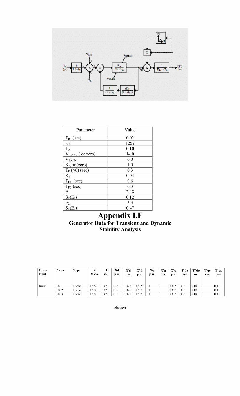
clxxxvi

Value Parameter

0.02 TR (sec) 1252 KA 0.10 TA 14.0 VRMAX ( or zero) 0.0 VRMIN 1.0 KE or (zero) 0.3 TE (>0) (sec)

0.03 KF 0.6 TF1 (sec) 0.3 TF2 (sec)

2.48 E1 0.12 SE(E1) 3.3 E2

0.47 SE(E2)

Appendix I.F Generator Data for Transient and Dynamic

Stability Analysis

Power Plant

Name Type S MVA

H sec

Xd p.u.

X′d p.u.

X″d p.u.

Xq p.u.

X′q p.u.

X″q p.u.

T′do sec

T″do sec

T′qo sec

T″qo sec

DG1 Diesel 12.8 1.42 1.75 0.325 0.215 1.1 0.375 3.9 0.04 0.1 DG2 Diesel 12.8 1.42 1.75 0.325 0.215 1.1 0.375 3.9 0.04 0.1

Burri

DG3 Diesel 12.8 1.42 1.75 0.325 0.215 1.1 0.375 3.9 0.04 0.1

clxxxvii

DG4 Diesel 12.8 1.42 1.75 0.325 0.215 1.1 0.375 3.9 0.04 0.1 DG5 Diesel 12.8 1.42 1.75 0.325 0.215 1.1 0.375 3.9 0.04 0.1 DG6 Diesel 12.8 1.42 1.75 0.325 0.215 1.1 0.375 3.9 0.04 0.1 G1 Diesel 1.25 1 1.27 0.355 0.21 0.89 0.18 2.7 0.039 0.08 G2 Diesel 1.25 1 1.27 0.355 0.21 0.89 0.18 2.7 0.039 0.08 G3 Diesel 1.25 1 1.27 0.355 0.21 0.89 0.18 2.7 0.039 0.08 G4 Diesel 1.25 1 1.27 0.355 0.205 0.89 0.18 2.7 0.039 0.08

Kassala

G5 Diesel 4.50 1.1 1.85 0.89 0.25 0.89 0.22 4.8 0.02 0.08 GT1 G.T. 23.5 7.92 2.16 0.20 0.142 2.10 0.3 0.15 5.34 0.05 0.59 0.06 GT2 G.T. 23.5 7.92 2.16 0.20 0.142 2.10 0.3 0.15 5.34 0.05 0.59 0.06 GT3 G.T. 25 7.92 2.16 0.20 0.142 2.10 0.3 0.15 5.34 0.05 0.59 0.06 GT4 G.T. 25 7.92 2.16 0.20 0.142 2.10 0.3 0.15 5.34 0.05 0.59 0.06 ST1 Steam 41.25 3.155 1.634 0.24 0.167 1.60 0.48 0.16 6.00 0.05 0.90 0.06 ST2 Steam 41.25 3.155 1.634 0.24 0.167 1.60 0.48 0.16 6.00 0.05 0.90 0.06 ST3 Steam 75 5.075 2.275 0.23 0.148 2.10 0.65 0.16 7.69 0.04 0.96 0.048

Kharto North

ST4 Steam 75 5.075 2.275 0.23 0.148 2.10 0.65 0.16 7.69 0.04 0.96 0.048 DG1 Diesel 4.50 1 1.85 0.89 0.235 0.89 0.22 4.8 0.02 0.08 DG2 Diesel 3.5 1.1 1.85 0.89 0.235 0.89 0.22 4.8 0.02 0.08 Kap.G1 Hydro 6.6 3.5 1.138 0.306 0.205 0.6832 0.12 6 0.05 0.1 Kap.G2 Hydro 6.6 3.5 1.138 0.306 0.205 0.6832 0.12 6 0.05 0.1 Pump.G1 Hydro 2.6 4 1.28 0.32 0.25 0.92 0.315 5.2 0.05 0.06 Pump.G2 Hydro 2.6 4 1.28 0.32 0.25 0.92 0.315 5.2 0.05 0.06

El Girba

Pump.G3 Hydro 2.6 4 1.28 0.32 0.25 0.92 0.315 5.2 0.05 0.06 Kuku GT1 G.T. 14.3 5 1.82 0.22 0.12 1 0.3 0.133 8.3 0.033 0.6 0.1

G1 Hydro 44.5 4.5 0.89 0.26 0.21 0.54 0.22 4.67 0.06 0.07 G2 Hydro 44.5 4.5 0.89 0.26 0.21 0.54 0.22 4.67 0.06 0.07 G3 Hydro 44.5 4.5 0.89 0.26 0.21 0.54 0.22 4.67 0.06 0.07 G4 Hydro 43 4.66 0.89 0.26 0.21 0.54 0.22 4.67 0.06 0.07 G5 Hydro 43 4.66 0.89 0.26 0.21 0.54 0.22 4.67 0.06 0.07 G6 Hydro 43 4.66 0.89 0.26 0.21 0.54 0.22 4.67 0.06 0.07

Roseires

G7 Hydro 43 4.66 0.89 0.26 0.21 0.54 0.22 4.67 0.06 0.07 G1 Hydro 9.4 2.22 1.02 0.3 0.2 0.65 0.25 5 0.041 0.074 Sennar G2 Hydro 9.4 2.22 1.02 0.3 0.2 0.65 0.25 5 0.041 0.074

Power

Plant

Name

Ra

p.u.

X1

p.u.

R2

p.u.

X2

p.u.

Ro

p.u.

Xo

p.u.

S(1.0)

S(1.2)

AVR

DG1 0.005 0.1 0.05 0.3 0.01 0.05 0.14 0.4 IEEET2 DG2 0.005 0.1 0.05 0.3 0.01 0.05 0.14 0.4 IEEET2 DG3 0.005 0.1 0.05 0.3 0.01 0.05 0.14 0.4 IEEET2 DG4 0.005 0.1 0.05 0.3 0.01 0.05 0.14 0.4 IEEET2 DG5 0.005 0.1 0.05 0.3 0.01 0.05 0.14 0.4 IEEET2

Burri

DG6 0.005 0.1 0.05 0.3 0.01 0.05 0.14 0.4 IEEET2 G1 0.005 0.13 0.05 0.2 0.01 0.05 0.14 0.5 IEEET2 G2 0.005 0.13 0.05 0.2 0.01 0.05 0.14 0.5 IEEET2 G3 0.005 0.13 0.05 0.2 0.01 0.05 0.14 0.5 IEEET2 G4 0.005 0.13 0.05 0.2 0.01 0.05 0.14 0.5 IEEET2

Kassala

G5 0.007 0.13 0.05 0.2 0.01 0.05 0.14 0.5 IEEET2 GT1 0.005 0.08 0.05 0.144 0.01 0.067 0.10 0.375 EXAC4 GT2 0.005 0.08 0.05 0.144 0.01 0.067 0.10 0.375 EXAC4 GT3 0.005 0.08 0.05 0.144 0.01 0.067 0.10 0.375 EXAC4 GT4 0.005 0.08 0.05 0.144 0.01 0.067 0.10 0.375 EXAC4 ST1 0.005 0.112 0.05 0.167 0.015 0.050 0.11 0.480 IEET5A ST2 0.005 0.112 0.05 0.167 0.015 0.050 0.11 0.480 IEET5A

Kharto North

ST3 0.005 0.10 0.05 0.153 0.015 0.091 0.11 0.463 ESDC1A

clxxxviii

ST4 0.005 0.10 0.05 0.153 0.015 0.091 0.11 0.463 ESDC1A DG1 0.007 0.13 0.05 0.2 0.01 0.05 0.14 0.5 IEEET2 DG2 0.007 0.13 0.05 0.2 0.01 0.05 0.14 0.5 IEEET2 Kap.G1 0.005 0.18 0.05 0.12 0.01 0.05 0.14 0.5 IEEET1 Kap.G2 0.005 0.18 0.05 0.12 0.01 0.05 0.14 0.5 IEEET1 Pump.G1 0.005 0.15 0.05 0.28 0.01 0.13 0.14 0.5 IEEET1 Pump.G2 0.005 0.15 0.05 0.28 0.01 0.13 0.14 0.5 IEEET1

El Girba

Pump.G3 0.005 0.15 0.05 0.28 0.01 0.13 0.14 0.5 IEEET1 Kuku GT1 0.005 0.1 0.05 0.13 0.01 0.06 0.14 0.5 IEEET2

G1 .0051 0.13 0.05 0.22 0.014 0.12 0.13 0.434 SCRX G2 .0051 0.13 0.05 0.22 0.014 0.12 0.13 0.434 SCRX G3 .0051 0.13 0.05 0.22 0.014 0.12 0.13 0.434 SCRX G4 .0051 0.13 0.05 0.24 0.014 0.12 0.13 0.434 SCRX G5 .0051 0.13 0.05 0.22 0.014 0.12 0.13 0.434 SCRX G6 .0051 0.13 0.05 0.22 0.014 0.12 0.13 0.434 SCRX

Roseires

G7 .0051 0.13 0.05 0.22 0.014 0.12 0.13 0.434 SCRX G1 .0075 0.16 0.05 0.205 0.014 0.13 0.11 0.48 IEEET1 Sennar G2 .0075 0.16 0.05 0.205 0.014 0.13 0.11 0.48 IEEET1

Appendix II

Appendix II.A Light Load

Load Flow Results

Busbar Name Voltage Generation Load MW MVAr MW MVAr 1 Burrold 1.061< -1.0 0.0 0.0 0.0 0.0 2 1.010< -1.0 0.0 0.0 0.0 0.0 3 Kuku 1.013< -0.9 0.0 0.0 23.5 14.1 4 1.022< 1.1 0.0 0.0 0.0 0.0 5 Khn1 1.020< 2.6 90.0 5.4 15.9 9.5 6 1.033< -0.5 0.0 0.0 0.0 0.0 7 1.023< -0.6 0.0 0.0 0.0 0.0 8 Khn2 1.074< -0.6 0.0 0.0 0.0 0.0 9 1.023< -0.7 0.0 0.0 0.0 0.0 10 El/Bashir 1.015< -1.3 0.0 0.0 0.0 0.0 11 KiloX 1.040< 0.0 13.1 9.5 0.0 0.0 12 Forest 1.017< -1.4 0.0 0.0 16.0 9.6 13 Magros 1.021< -1.3 0.0 0.0 28.0 16.8 14 KiloXL1 1.033< -0.6 0.0 0.0 1.1 0.7 15 1.030< -0.8 0.0 0.0 0.0 0.0 16 OmdurL1 1.003< -2.4 0.0 0.0 18.0 10.8 17 1.041< -0.5 0.0 0.0 0.0 0.0 18 1.047< -0.3 0.0 0.0 0.0 0.0 19 1.029< -0.8 0.0 0.0 0.0 0.0 20 Bager 1.034< -0.8 0.0 0.0 0.0 0.0 21 EL-BagL1 0.979< -1.3 0.0 0.0 4.3 2.6 22 EL-BagL2 0.978< -1.5 0.0 0.0 4.3 2.6 23 Maringan 1.073< 0.9 0.0 0.0 0.0 0.0

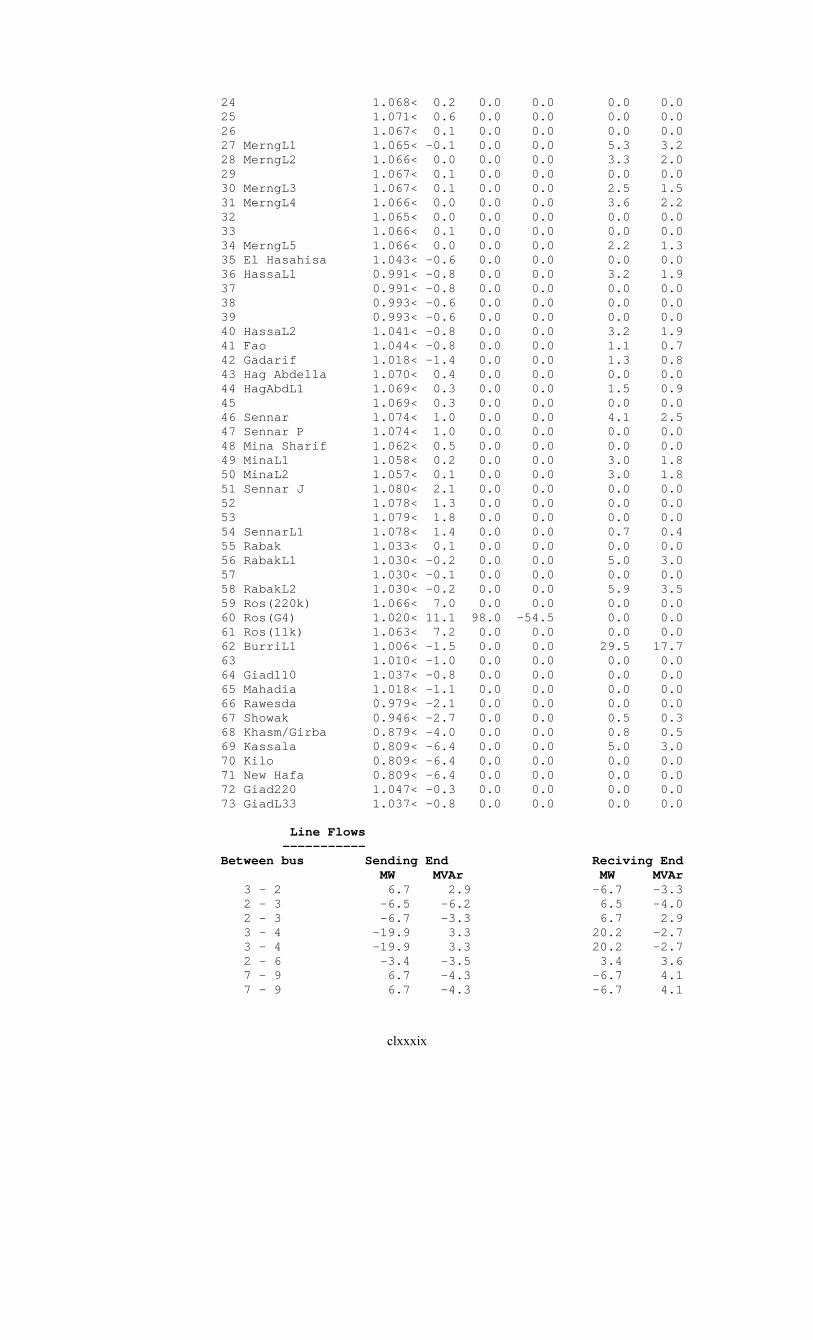
clxxxix

24 1.068< 0.2 0.0 0.0 0.0 0.0 25 1.071< 0.6 0.0 0.0 0.0 0.0 26 1.067< 0.1 0.0 0.0 0.0 0.0 27 MerngL1 1.065< -0.1 0.0 0.0 5.3 3.2 28 MerngL2 1.066< 0.0 0.0 0.0 3.3 2.0 29 1.067< 0.1 0.0 0.0 0.0 0.0 30 MerngL3 1.067< 0.1 0.0 0.0 2.5 1.5 31 MerngL4 1.066< 0.0 0.0 0.0 3.6 2.2 32 1.065< 0.0 0.0 0.0 0.0 0.0 33 1.066< 0.1 0.0 0.0 0.0 0.0 34 MerngL5 1.066< 0.0 0.0 0.0 2.2 1.3 35 El Hasahisa 1.043< -0.6 0.0 0.0 0.0 0.0 36 HassaL1 0.991< -0.8 0.0 0.0 3.2 1.9 37 0.991< -0.8 0.0 0.0 0.0 0.0 38 0.993< -0.6 0.0 0.0 0.0 0.0 39 0.993< -0.6 0.0 0.0 0.0 0.0 40 HassaL2 1.041< -0.8 0.0 0.0 3.2 1.9 41 Fao 1.044< -0.8 0.0 0.0 1.1 0.7 42 Gadarif 1.018< -1.4 0.0 0.0 1.3 0.8 43 Hag Abdella 1.070< 0.4 0.0 0.0 0.0 0.0 44 HagAbdL1 1.069< 0.3 0.0 0.0 1.5 0.9 45 1.069< 0.3 0.0 0.0 0.0 0.0 46 Sennar 1.074< 1.0 0.0 0.0 4.1 2.5 47 Sennar P 1.074< 1.0 0.0 0.0 0.0 0.0 48 Mina Sharif 1.062< 0.5 0.0 0.0 0.0 0.0 49 MinaL1 1.058< 0.2 0.0 0.0 3.0 1.8 50 MinaL2 1.057< 0.1 0.0 0.0 3.0 1.8 51 Sennar J 1.080< 2.1 0.0 0.0 0.0 0.0 52 1.078< 1.3 0.0 0.0 0.0 0.0 53 1.079< 1.8 0.0 0.0 0.0 0.0 54 SennarL1 1.078< 1.4 0.0 0.0 0.7 0.4 55 Rabak 1.033< 0.1 0.0 0.0 0.0 0.0 56 RabakL1 1.030< -0.2 0.0 0.0 5.0 3.0 57 1.030< -0.1 0.0 0.0 0.0 0.0 58 RabakL2 1.030< -0.2 0.0 0.0 5.9 3.5 59 Ros(220k) 1.066< 7.0 0.0 0.0 0.0 0.0 60 Ros(G4) 1.020< 11.1 98.0 -54.5 0.0 0.0 61 Ros(11k) 1.063< 7.2 0.0 0.0 0.0 0.0 62 BurriL1 1.006< -1.5 0.0 0.0 29.5 17.7 63 1.010< -1.0 0.0 0.0 0.0 0.0 64 Giad110 1.037< -0.8 0.0 0.0 0.0 0.0 65 Mahadia 1.018< -1.1 0.0 0.0 0.0 0.0 66 Rawesda 0.979< -2.1 0.0 0.0 0.0 0.0 67 Showak 0.946< -2.7 0.0 0.0 0.5 0.3 68 Khasm/Girba 0.879< -4.0 0.0 0.0 0.8 0.5 69 Kassala 0.809< -6.4 0.0 0.0 5.0 3.0 70 Kilo 0.809< -6.4 0.0 0.0 0.0 0.0 71 New Hafa 0.809< -6.4 0.0 0.0 0.0 0.0 72 Giad220 1.047< -0.3 0.0 0.0 0.0 0.0 73 GiadL33 1.037< -0.8 0.0 0.0 0.0 0.0

Line Flows -----------

Between bus Sending End Reciving End MW MVAr MW MVAr 3 - 2 6.7 2.9 -6.7 -3.3 2 - 3 -6.5 -6.2 6.5 -4.0 2 - 3 -6.7 -3.3 6.7 2.9 3 - 4 -19.9 3.3 20.2 -2.7 3 - 4 -19.9 3.3 20.2 -2.7 2 - 6 -3.4 -3.5 3.4 3.6 7 - 9 6.7 -4.3 -6.7 4.1 7 - 9 6.7 -4.3 -6.7 4.1

cxc

10 - 12 2.2 -3.2 -2.2 2.8 12 - 13 -13.8 -12.4 13.8 12.1 9 - 15 1.8 -15.6 -1.8 15.3 9 - 15 1.8 -15.6 -1.8 15.3 13 - 15 -41.8 -28.9 42.0 29.0 2 - 3 -6.2 -1.6 6.2 0.2 15 - 20 -7.6 -14.5 7.6 14.1 18 - 23 -18.4 -28.5 18.5 2.0 24 - 35 8.1 1.4 -8.0 -4.1 24 - 41 10.1 2.8 -9.9 -5.2 41 - 42 8.8 4.6 -8.7 -6.0 24 - 43 -3.1 -0.1 3.2 -1.3 43 - 46 -4.7 0.4 4.7 -2.6 46 - 48 6.1 1.2 -6.0 -3.7 23 - 51 -34.6 -9.3 34.7 -3.4 23 - 51 -34.6 -9.3 34.7 -3.4 52 - 46 14.9 -1.4 -14.8 -1.1 52 - 55 11.3 3.5 -10.9 -6.6 51 - 59 -48.2 2.0 49.0 -32.1 51 - 59 -48.2 2.0 49.0 -32.1 64 - 20 16.2 19.4 -16.2 -19.4 64 - 35 -1.6 -1.5 1.6 0.2 7 - 65 20.3 6.7 -20.2 -7.4 10 - 65 -20.2 -8.1 20.2 7.4 42 - 66 7.4 5.2 -7.1 -5.0 66 - 67 7.1 5.0 -7.0 -4.7 67 - 68 6.5 4.4 -6.1 -4.0 68 - 69 5.3 3.5 -5.0 -3.0 69 - 70 0.0 0.0 0.0 0.0 70 - 71 0.0 0.0 0.0 0.0 23 - 72 18.7 1.8 -18.5 -28.3 18 - 72 -3.9 -12.7 3.9 10.0

2-Winding Transformer Flows -----------

Between Bus Primary Secondary MW MVAr MW MVAr

1 - 2 0.0 0.0 0.0 0.0 5 - 4 74.1 -4.1 -74.1 6.1 4 - 7 33.8 -0.8 -33.8 1.8 8 - 7 0.0 0.0 0.0 0.0 3 - 9 -5.0 -11.4 5.0 11.6 6 - 11 -13.1 -9.3 13.1 9.5 10 - 16 18.0 11.3 -18.0 -10.8 24 - 27 5.3 3.2 -5.3 -3.2 24 - 28 3.3 2.0 -3.3 -2.0 35 - 40 3.2 1.9 -3.2 -1.9 46 - 47 0.0 0.0 0.0 0.0 55 - 58 5.9 3.6 -5.9 -3.5 62 - 2 -29.5 -17.7 29.5 18.0 3 - 9 -5.0 -11.4 5.0 11.6 63 - 2 0.0 0.0 0.0 0.0 64 - 73 0.3 0.4 -0.3 -0.4

3-Winding Transformer Flows -----------

Between Bus Primary Secondary Tertiary MW MVAr MW MVAr MW MVAr 15 - 6 - 14 -8.6 -5.0 9.7 5.7 -1.1 -0.7 18 - 17 - 15 5.9 10.9 0.0 0.0 -5.9 -10.7 18 - 15 - 19 16.4 30.3 -16.4 -29.6 0.0 0.0 20 - 21 - 22 8.6 5.3 -4.3 -2.6 -4.3 -2.6 23 - 24 - 26 23.2 10.7 -23.2 -10.4 0.0 0.0

cxci

23 - 25 - 24 8.7 4.0 0.0 0.0 -8.7 -3.9 24 - 29 - 30 2.5 1.5 0.0 0.0 -2.5 -1.5 24 - 31 - 32 3.6 2.2 -3.6 -2.2 0.0 0.0 24 - 33 - 34 2.2 1.3 0.0 0.0 -2.2 -1.3 35 - 36 - 37 3.2 1.9 -3.2 -1.9 0.0 0.0 35 - 38 - 39 0.0 0.0 0.0 0.0 0.0 0.0 43 - 44 - 45 1.5 0.9 -1.5 -0.9 0.0 0.0 48 - 49 - 50 6.0 3.7 -3.0 -1.8 -3.0 -1.8 51 - 53 - 52 6.5 0.7 0.0 0.0 -6.5 -0.6 51 - 52 - 54 20.4 2.2 -19.7 -1.5 -0.7 -0.4 55 - 56 - 57 5.0 3.1 -5.0 -3.0 0.0 0.0 59 - 60 - 61 -98.0 64.2 98.0 -54.5 0.0 0.0 72 - 64 - 73 14.7 18.2 -15.0 -18.3 0.3 0.4

Transimission Losses = 5.33MWs Number Of Iterations = 5

Appendix II.B Medium Load

Load Flow Results

Busbar Name Voltage Generation Load MW MVAr MW MVAr

1 Burrold 1.028< -8.7 0.0 0.0 0.0 0.0 2 0.979< -8.7 0.0 0.0 0.0 0.0 3 Kuku 0.985< -8.6 0.0 0.0 27.1 16.3 4 1.010< -6.6 0.0 0.0 0.0 0.0 5 Khn1 1.020< -5.2 90.0 39.5 20.4 12.2 6 1.018< -4.6 0.0 0.0 0.0 0.0 7 0.998< -8.0 0.0 0.0 0.0 0.0 8 Khn2 1.048< -8.0 0.0 0.0 0.0 0.0 9 0.998< -8.0 0.0 0.0 0.0 0.0 10 El/Bashir 0.982< -9.1 0.0 0.0 0.0 0.0 11 KiloX 1.040< 0.0 110.7 34.7 0.0 0.0 12 Forest 0.985< -9.1 0.0 0.0 41.5 12.9 13 Magros 0.992< -8.6 0.0 0.0 37.5 22.5 14 KiloXL1 1.017< -4.5 0.0 0.0 2.3 1.4 15 1.007< -7.7 0.0 0.0 0.0 0.0 16 OmdurL1/2 0.958<-11.4 0.0 0.0 33.0 19.8 17 1.017< -7.4 0.0 0.0 0.0 0.0 18 1.024< -7.3 0.0 0.0 0.0 0.0 19 1.005< -7.7 0.0 0.0 0.0 0.0 20 Bager 1.010< -7.7 0.0 0.0 0.0 0.0 21 EL-BagL1 0.957< -8.2 0.0 0.0 4.2 2.5 22 EL-BagL2 0.955< -8.4 0.0 0.0 4.2 2.5 23 Maringan 1.050< -6.5 0.0 0.0 0.0 0.0 24 1.043< -7.4 0.0 0.0 0.0 0.0 25 1.047< -6.8 0.0 0.0 0.0 0.0 26 1.042< -7.4 0.0 0.0 0.0 0.0 27 MerngL1 1.039< -7.7 0.0 0.0 5.7 3.4 28 MerngL2 1.040< -7.6 0.0 0.0 4.2 2.5 29 1.041< -7.5 0.0 0.0 0.0 0.0 30 MerngL3 1.042< -7.4 0.0 0.0 3.0 1.8 31 MerngL4 1.040< -7.6 0.0 0.0 4.8 2.9 32 1.040< -7.6 0.0 0.0 0.0 0.0 33 1.040< -7.5 0.0 0.0 0.0 0.0 34 MerngL5 1.039< -7.6 0.0 0.0 3.5 2.1 35 El Hasahisa 1.011< -8.0 0.0 0.0 0.0 0.0

cxcii

36 HassaL1 0.959< -8.4 0.0 0.0 5.0 3.0 37 0.959< -8.4 0.0 0.0 0.0 0.0 38 0.963< -8.0 0.0 0.0 0.0 0.0 39 0.963< -8.0 0.0 0.0 0.0 0.0 40 HassaL2 1.008< -8.3 0.0 0.0 5.0 3.0 41 Fao 1.014< -8.6 0.0 0.0 1.9 1.1 42 Gadarif 0.987< -9.5 0.0 0.0 4.1 2.5 43 Hag Abdella 1.046< -7.1 0.0 0.0 0.0 0.0 44 HagAbdL1 1.045< -7.2 0.0 0.0 1.2 0.8 45 1.045< -7.2 0.0 0.0 0.0 0.0 46 Sennar 1.052< -6.5 0.0 0.0 4.3 2.6 47 Sennar P 1.052< -6.5 0.0 0.0 0.0 0.0 48 Mina Sharif 1.038< -7.0 0.0 0.0 0.0 0.0 49 MinaL1 1.034< -7.4 0.0 0.0 3.3 2.0 50 MinaL2 1.033< -7.5 0.0 0.0 3.0 1.8 51 Sennar J 1.060< -5.3 0.0 0.0 0.0 0.0 52 1.057< -6.2 0.0 0.0 0.0 0.0 53 1.059< -5.7 0.0 0.0 0.0 0.0 54 SennarL1 1.057< -6.1 0.0 0.0 0.4 0.2 55 Rabak 1.001< -7.6 0.0 0.0 0.0 0.0 56 RabakL1 0.997< -7.9 0.0 0.0 5.8 3.5 57 0.998< -7.9 0.0 0.0 0.0 0.0 58 RabakL2 0.997< -8.0 0.0 0.0 6.8 4.1 59 Ros(220k) 1.056< -0.5 0.0 0.0 0.0 0.0 60 Ros(G4) 1.020< 3.7 98.0 -42.0 0.0 0.0 61 Ros(11k) 1.053< -0.3 0.0 0.0 1.6 1.0 62 BurriL1 0.971< -9.5 0.0 0.0 53.4 32.0 63 0.979< -8.7 0.0 0.0 0.0 0.0 64 Giad110 1.013< -7.7 0.0 0.0 0.0 0.0 65 Mahadia 0.987< -8.8 0.0 0.0 0.0 0.0 66 Rawesda 0.958<-10.1 0.0 0.0 0.0 0.0 67 Showak 0.934<-10.7 0.0 0.0 0.6 0.4 68 Khasm/Girba 0.889<-12.0 0.0 0.0 0.9 0.0 69 Kassala 0.840<-13.6 0.0 0.0 3.6 2.2 70 Kilo 0.840<-13.6 0.0 0.0 0.0 0.0 71 New Hafa 0.840<-13.6 0.0 0.0 0.0 0.0 72 Giad220 1.024< -7.3 0.0 0.0 0.0 0.0 73 GiadL33 1.013< -7.7 0.0 0.0 0.0 0.0

Line Flows ----------- Between bus Sending End Reciving End

MW MVAr MW MVAr 3 - 2 9.3 8.2 -9.3 -8.5 2 - 3 -10.0 -9.8 10.0 0.2 2 - 3 -9.3 -8.5 9.3 8.2 3 - 4 -21.7 -5.0 22.0 5.8 3 - 4 -21.7 -5.0 22.0 5.8 2 - 6 -15.3 -1.0 15.8 2.2 7 - 9 -3.9 -1.6 3.9 1.4 7 - 9 -3.9 -1.6 3.9 1.4 10 - 12 0.1 -4.9 -0.1 4.6 12 - 13 -41.4 -17.5 41.5 17.6 9 - 15 -14.9 -15.1 15.0 14.9 9 - 15 -14.9 -15.1 15.0 14.9 13 - 15 -79.0 -40.1 79.5 41.6 2 - 3 -9.6 -5.2 9.6 3.9 15 - 20 -2.1 -14.9 2.2 14.6 18 - 23 -13.4 -28.7 13.5 3.3 24 - 35 8.5 3.4 -8.3 -5.9 24 - 41 12.1 3.4 -11.8 -5.6 41 - 42 9.9 4.4 -9.8 -5.7

cxciii

24 - 43 -3.6 -0.7 3.6 -0.6 43 - 46 -4.8 -0.1 4.9 -2.0 46 - 48 6.4 1.5 -6.3 -3.8 23 - 51 -32.7 -13.1 32.8 0.9 23 - 51 -32.7 -13.1 32.8 0.9 52 - 46 15.6 -0.3 -15.5 -2.1 52 - 55 13.2 4.9 -12.6 -7.7 51 - 59 -47.4 -3.6 48.2 -25.9 51 - 59 -47.4 -3.6 48.2 -25.9 64 - 20 10.6 19.8 -10.6 -19.8 64 - 35 1.7 -1.1 -1.7 -0.1 7 - 65 33.3 16.0 -33.2 -16.2 10 - 65 -33.1 -16.7 33.2 16.2 42 - 66 5.7 3.3 -5.5 -3.1 66 - 67 5.5 3.1 -5.4 -3.0 67 - 68 4.8 2.6 -4.6 -2.4 68 - 69 3.7 2.4 -3.6 -2.2 69 - 70 0.0 0.0 0.0 0.0 70 - 71 0.0 0.0 0.0 0.0 23 - 72 13.7 3.2 -13.6 -28.6 18 - 72 -1.3 -12.1 1.3 9.6

2-Winding Transformer Flows -----------

Between Bus Primary Secondary MW MVAr MW MVAr

1 - 2 0.0 0.0 0.0 0.0 5 - 4 69.6 27.3 -69.6 -25.2 4 - 7 25.6 13.6 -25.6 -12.8 8 - 7 0.0 0.0 0.0 0.0 3 - 9 -11.0 -13.4 11.0 13.7 6 - 11 -110.6 -25.1 110.6 34.7 10 - 16 33.0 21.6 -33.0 -19.8 24 - 27 5.7 3.5 -5.7 -3.4 24 - 28 4.2 2.5 -4.2 -2.5 35 - 40 5.0 3.0 -5.0 -3.0 46 - 47 0.0 0.0 0.0 0.0 55 - 58 6.8 4.1 -6.8 -4.1 62 - 2 -53.4 -32.0 53.4 33.1 3 - 9 -11.0 -13.4 11.0 13.7 63 - 2 0.0 0.0 0.0 0.0 64 - 73 0.3 0.4 -0.3 -0.4

3-Winding Transformer Flows -----------

Between Bus Primary Secondary Tertiary MW MVAr MW MVAr MW MVAr 15 - 6 - 14 -92.6 -16.4 94.9 22.9 -2.3 -1.4 18 - 17 - 15 3.9 10.8 0.0 0.0 -3.9 -10.6 18 - 15 - 19 10.8 30.0 -10.8 -29.5 0.0 0.0 20 - 21 - 22 8.4 5.2 -4.2 -2.5 -4.2 -2.5 23 - 24 - 26 27.7 14.4 -27.7 -13.8 0.0 0.0 23 - 25 - 24 10.4 5.4 0.0 0.0 -10.4 -5.2 24 - 29 - 30 3.0 1.8 0.0 0.0 -3.0 -1.8 24 - 31 - 32 4.8 2.9 -4.8 -2.9 0.0 0.0 24 - 33 - 34 3.5 2.1 0.0 0.0 -3.5 -2.1 35 - 36 - 37 5.0 3.0 -5.0 -3.0 0.0 0.0 35 - 38 - 39 0.0 0.0 0.0 0.0 0.0 0.0 43 - 44 - 45 1.2 0.8 -1.2 -0.7 0.0 0.0 48 - 49 - 50 6.3 3.8 -3.3 -2.0 -3.0 -1.8 51 - 53 - 52 7.0 1.3 0.0 0.0 -7.0 -1.2 51 - 52 - 54 22.1 4.1 -21.7 -3.5 -0.4 -0.2 55 - 56 - 57 5.8 3.5 -5.8 -3.5 0.0 0.0

cxciv

59 - 60 - 61 -96.4 51.7 98.0 -42.0 -1.6 -1.0 72 - 64 - 73 12.3 19.0 -12.6 -19.1 0.3 0.4

Transimission Losses = 6.34MWs Number Of Iterations = 4

Appendix II.C Peak Load

Load Flow Results

Busbar Name Voltage Generation Load MW MVAr MW MVAr

1 Burrold 0.980< -1.0 0.0 0.0 0.0 0.0 2 0.933< -1.0 0.0 0.0 0.0 0.0 3 Kuku 0.939< -0.7 0.0 0.0 52.9 31.7 4 0.991< 4.5 0.0 0.0 0.0 0.0 5 Khn1 1.020< 8.7 196.0 83.9 0.0 0.0 6 0.989< -0.6 0.0 0.0 0.0 0.0 7 KhartoumN 0.952< -0.6 0.0 0.0 25.5 15.3 8 Khn2 1.000< -0.6 0.0 0.0 0.0 0.0 9 0.952< -0.7 0.0 0.0 0.0 0.0 10 El/Bashir 0.921< -2.5 0.0 0.0 0.0 0.0 11 KiloX 1.040< 0.0 14.4 69.2 0.0 0.0 12 Forest 0.925< -2.5 0.0 0.0 33.5 20.1 13 Magros 0.934< -2.1 0.0 0.0 60.0 36.0 14 KiloXL1 0.990< -0.7 0.0 0.0 1.6 0.9 15 0.956< -0.9 0.0 0.0 0.0 0.0 16 OmdurL1 0.879< -6.6 0.0 0.0 51.6 31.0 17 0.962< 0.0 0.0 0.0 0.0 0.0 18 0.967< 0.6 0.0 0.0 0.0 0.0 19 0.955< -1.0 0.0 0.0 0.0 0.0 20 Bager 0.959< -0.6 0.0 0.0 0.0 0.0 21 EL-BagL1 0.914< -1.5 0.0 0.0 6.2 3.7 22 EL-BagL2 0.912< -1.8 0.0 0.0 6.2 3.7 23 Maringan 0.988< 4.4 0.0 0.0 0.0 0.0 24 0.981< 3.0 0.0 0.0 0.0 0.0 25 0.985< 3.9 0.0 0.0 0.0 0.0 26 0.981< 2.9 0.0 0.0 0.0 0.0 27 MerngL1 0.977< 2.7 0.0 0.0 6.1 3.6 28 MerngL2 0.978< 2.7 0.0 0.0 5.2 3.1 29 0.980< 2.9 0.0 0.0 0.0 0.0 30 MerngL3 0.980< 2.9 0.0 0.0 3.6 2.2 31 MerngL4 0.985< 2.4 0.0 0.0 10.1 6.0 32 0.991< 2.4 0.0 0.0 0.0 0.0 33 0.977< 2.6 0.0 0.0 0.0 0.0 34 MerngL5 0.974< 2.3 0.0 0.0 7.4 4.4 35 El Hasahisa 0.960< 0.0 0.0 0.0 0.0 0.0 36 HassaL1 0.920< -0.4 0.0 0.0 6.4 3.8 37 0.924< -0.4 0.0 0.0 0.0 0.0 38 0.914< 0.0 0.0 0.0 0.0 0.0 39 0.914< 0.0 0.0 0.0 0.0 0.0 40 HassaL2 0.956< -0.3 0.0 0.0 6.4 3.8 41 Fao 0.946< 1.5 0.0 0.0 2.7 1.6 42 Gadarif 0.915< 0.3 0.0 0.0 6.2 3.7 43 Hag Abdella 0.980< 3.8 0.0 0.0 0.0 0.0 44 HagAbdL1 0.979< 3.6 0.0 0.0 2.6 1.6 45 0.979< 3.6 0.0 0.0 0.0 0.0 46 Sennar 0.984< 5.4 0.0 0.0 1.2 0.7

cxcv

47 Sennar P 0.984< 5.4 0.0 0.0 0.0 0.0 48 Mina Sharif 0.950< 4.3 0.0 0.0 0.0 0.0 49 MinaL1 0.942< 3.5 0.0 0.0 6.0 3.6 50 MinaL2 0.939< 3.3 0.0 0.0 6.0 4.0 51 Sennar J 0.997< 7.4 0.0 0.0 0.0 0.0 52 0.990< 5.8 0.0 0.0 0.0 0.0 53 0.995< 6.9 0.0 0.0 0.0 0.0 54 SennarL1 0.987< 5.7 0.0 0.0 4.5 2.7 55 Rabak 0.898< 3.8 0.0 0.0 0.0 0.0 56 RabakL1 0.892< 3.1 0.0 0.0 8.3 5.0 57 0.893< 3.2 0.0 0.0 0.0 0.0 58 RabakL2 0.891< 3.1 0.0 0.0 9.7 5.8 59 Ros(220k) 1.024< 17.9 0.0 0.0 0.0 0.0 60 Ros(G4) 1.020< 26.7 200.0 10.3 0.0 0.0 61 Ros(11k) 1.022< 18.3 0.0 0.0 2.7 1.6 62 BurriL1 0.924< -1.9 0.0 0.0 54.6 32.7 63 0.933< -1.0 0.0 0.0 0.0 0.0 64 Giad110 0.963< -0.4 0.0 0.0 0.0 0.0 65 Mahadia 0.931< -1.9 0.0 0.0 0.0 0.0 66 Rawesda 0.894< -0.5 0.0 0.0 0.0 0.0 67 Showak 0.877< -1.1 0.0 0.0 0.4 0.2 68 Khasm/Girba 0.843< -2.5 0.0 0.0 1.4 0.9 69 Kassala 0.823< -4.1 0.0 0.0 2.3 0.4 70 Kilo 0.823< -4.1 0.0 0.0 0.0 0.0 71 New Halfa 0.823< -4.1 0.0 0.0 0.0 0.0 72 0.968< 0.7 0.0 0.0 0.0 0.0 73 GiadL33 0.963< -0.5 0.0 0.0 0.0 0.0

Line Flows ----------- Between bus Sending End Reciving End

MW MVAr MW MVAr 3 - 2 12.9 4.5 -12.9 -4.8 2 - 3 -12.3 -5.4 12.3 -3.3 2 - 3 -12.9 -4.8 12.9 4.5 3 - 4 -51.0 -5.5 53.1 10.6 3 - 4 -51.0 -5.5 53.1 10.6 2 - 6 -4.9 -8.9 5.1 9.5 7 - 9 6.1 -1.0 -6.1 0.8 7 - 9 6.1 -1.0 -6.1 0.8 10 - 12 -0.2 -5.4 0.2 5.1 12 - 13 -33.7 -25.2 33.9 25.4 9 - 15 5.7 -9.7 -5.6 9.4 9 - 15 5.7 -9.7 -5.6 9.4 13 - 15 -93.8 -61.4 94.7 64.5 2 - 3 -11.7 -1.3 11.7 0.1 15 - 20 -20.2 -7.4 20.2 7.2 18 - 23 -44.1 -15.8 44.7 -4.3 24 - 35 14.5 -5.1 -13.9 3.3 24 - 41 13.9 4.5 -13.5 -6.2 41 - 42 10.8 4.5 -10.6 -5.5 24 - 43 -5.8 5.0 5.8 -6.0 43 - 46 -8.4 4.5 8.6 -6.2 46 - 48 12.3 6.3 -12.0 -7.9 23 - 51 -71.5 -3.2 72.3 -4.5 23 - 51 -71.5 -3.2 72.3 -4.5 52 - 46 22.2 -1.2 -22.0 -0.8 52 - 55 19.4 9.9 -17.9 -11.0 51 - 59 -95.3 -1.9 98.6 -11.1 51 - 59 -95.3 -1.9 98.6 -11.1 64 - 20 32.7 6.6 -32.6 -6.5 64 - 35 -1.1 1.5 1.1 -2.6

cxcvi

7 - 65 52.1 32.1 -51.6 -31.0 10 - 65 -51.4 -30.8 51.6 31.0 42 - 66 4.4 1.8 -4.3 -1.7 66 - 67 4.3 1.7 -4.2 -1.6 67 - 68 3.8 1.4 -3.7 -1.3 69 - 70 0.0 0.0 0.0 0.0 70 - 71 0.0 0.0 0.0 0.0 68 - 69 2.3 0.4 -2.3 -0.3 23 - 72 43.6 -5.1 -43.0 -15.1 18 - 72 -11.4 -8.5 11.4 6.3

2-Winding Transformer Flows -----------

Between Bus Primary Secondary MW MVAr MW MVAr

1 - 2 0.0 0.0 0.0 0.0 5 - 4 196.0 84.0 -196.0 -67.3 4 - 7 89.7 46.1 -89.7 -36.4 8 - 7 0.0 0.0 0.0 0.0 3 - 9 -0.4 -13.3 0.4 13.5 6 - 11 -14.4 -65.6 14.4 69.2 10 - 16 51.6 36.2 -51.6 -31.0 24 - 27 6.1 3.7 -6.1 -3.6 24 - 28 5.2 3.1 -5.2 -3.1 35 - 40 6.4 3.9 -6.4 -3.8 46 - 47 0.0 0.0 0.0 0.0 55 - 58 9.7 5.9 -9.7 -5.8 62 - 2 -54.6 -32.7 54.6 33.9 3 - 9 -0.4 -13.3 0.4 13.5 63 - 2 0.0 0.0 0.0 0.0 73 - 64 -0.7 -0.2 0.7 0.2

3-Winding Transformer Flows -----------

Between Bus Primary Secondary Tertiary MW MVAr MW MVAr MW MVAr 15 - 6 - 14 -7.7 -53.3 9.3 56.1 -1.6 -0.9 18 - 17 - 15 14.7 6.4 0.0 0.0 -14.7 -6.0 18 - 15 - 19 40.8 17.9 -40.8 -16.6 0.0 0.0 20 - 21 - 22 12.4 -0.7 -6.2 4.6 -6.2 -3.7 23 - 24 - 26 39.8 11.4 -39.8 -10.4 0.0 0.0 23 - 25 - 24 15.0 4.3 0.0 0.0 -15.0 -3.9 24 - 29 - 30 3.6 2.2 0.0 0.0 -3.6 -2.2 24 - 31 - 32 10.1 -3.6 -10.1 -6.0 0.0 9.8 24 - 33 - 34 7.4 4.5 0.0 0.0 -7.3 -4.4 35 - 36 - 37 6.4 -4.6 -6.4 -3.8 0.0 8.5 35 - 38 - 39 0.0 0.0 0.0 0.0 0.0 0.0 43 - 44 - 45 2.6 1.6 -2.6 -1.5 0.0 0.0 48 - 49 - 50 12.0 7.9 -6.0 -3.6 -6.0 -4.0 51 - 53 - 52 10.9 3.0 0.0 0.0 -10.9 -2.6 51 - 52 - 54 35.1 9.8 -30.6 -6.1 -4.5 -2.7 55 - 56 - 57 8.3 5.1 -8.3 -5.0 0.0 0.0 59 - 60 - 61 -197.3 22.1 200.0 10.3 -2.7 -1.6 72 - 64 - 73 31.6 8.8 -32.3 -8.3 0.7 0.2

Transimission Losses = 19.40MWs Number Of Iterations = 5

Appendix II.D Light Load (2006) Load Flow Results

cxcvii

Busbar Name Voltage Generation Load MW MVAr MW MVAr

1 Burrold 0.909<-12.5 0.0 0.0 26.9 35.8 2 0.913<-10.3 0.0 0.0 0.0 0.0 3 Kuku 0.923<-10.2 0.0 0.0 27.3 20.5 4 0.985< -7.5 0.0 0.0 0.0 0.0 5 Khn1 1.020< -5.2 150.0 130.4 44.1 33.1 6 0.965< -6.5 0.0 0.0 0.0 0.0 7 0.941< -9.7 0.0 0.0 0.0 0.0 8 Khn2 0.989< -9.7 0.0 0.0 0.0 0.0 9 0.939< -9.8 0.0 0.0 0.0 0.0 10 El/Bashir 0.818<-11.5 0.0 0.0 0.0 0.0 11 KiloX 1.040< 0.0 147.4 109.5 0.0 0.0 12 Forest 0.875<-11.2 0.0 0.0 8.8 2.0 13 Magros 0.895<-11.2 0.0 0.0 77.5 50.7 14 KiloXL1 0.947< -8.3 0.0 0.0 35.0 20.2 15 0.932<-10.1 0.0 0.0 0.0 0.0 16 OmdurL1 0.771<-15.6 0.0 0.0 41.1 30.9 17 0.944< -9.9 0.0 0.0 0.0 0.0 18 0.952< -9.8 0.0 0.0 0.0 0.0 19 0.931<-10.1 0.0 0.0 0.0 0.0 20 Bager 0.931<-10.6 0.0 0.0 0.0 0.0 21 EL-BagL1 0.862<-12.7 0.0 0.0 17.5 12.0 22 EL-BagL2 0.856<-13.2 0.0 0.0 10.0 8.0 23 Maringan 0.983< -9.0 0.0 0.0 0.0 0.0 24 0.967<-11.1 0.0 0.0 0.0 0.0 25 0.977< -9.8 0.0 0.0 0.0 0.0 26 0.966<-11.2 0.0 0.0 0.0 0.0 27 MerngL1 0.959<-11.7 0.0 0.0 10.0 8.0 28 MerngL2 0.957<-11.8 0.0 0.0 13.0 10.0 29 0.961<-11.5 0.0 0.0 0.0 0.0 30 MerngL3 0.963<-11.4 0.0 0.0 9.0 7.5 31 MerngL4 0.952<-12.4 0.0 0.0 20.0 14.5 32 0.951<-12.4 0.0 0.0 0.0 0.0 33 0.967<-11.2 0.0 0.0 0.0 0.0 34 MerngL5 0.966<-11.3 0.0 0.0 1.7 0.4 35 El Hasahisa 0.919<-13.0 0.0 0.0 0.0 0.0 36 HassaL1 0.859<-14.3 0.0 0.0 16.0 13.0 37 0.858<-14.3 0.0 0.0 0.0 0.0 38 0.894<-13.0 0.0 0.0 0.0 0.0 39 0.904<-13.0 0.0 0.0 0.0 0.0 40 HassaL2 0.913<-13.5 0.0 0.0 8.0 5.8 41 Fao 0.941<-14.7 0.0 0.0 3.4 2.6 42 Gadarif 0.930<-19.0 0.0 0.0 6.9 5.2 43 Hag Abdella 0.982<-10.9 0.0 0.0 0.0 0.0 44 HagAbdL1 0.978<-11.3 0.0 0.0 5.5 4.3 45 0.978<-11.3 0.0 0.0 0.0 0.0 46 Sennar 1.024<-10.3 0.0 0.0 15.6 11.7 47 Sennar P 1.080< -9.5 14.0 53.6 0.0 0.0 48 Mina Sharif 0.983<-11.9 0.0 0.0 0.0 0.0 49 MinaL1 0.974<-12.9 0.0 0.0 17.3 13.0 50 MinaL2 0.976<-13.0 0.0 0.0 0.0 0.0 51 Sennar J 1.005< -6.8 0.0 0.0 0.0 0.0 52 1.026< -9.3 0.0 0.0 0.0 0.0 53 1.012< -7.6 0.0 0.0 0.0 0.0 54 SennarL1 1.008< -9.9 0.0 0.0 11.3 8.4 55 Rabak 1.001<-17.8 0.0 0.0 0.0 0.0 56 RabakL1 1.019<-19.0 0.0 0.0 20.0 19.0

cxcviii

57 1.028<-18.8 0.0 0.0 0.0 0.0 58 RabakL2 0.995<-18.3 0.0 0.0 8.8 5.6 59 Ros(220k) 1.028< 3.7 0.0 0.0 0.0 0.0 60 Ros(G4) 1.020< 12.5 200.0 5.4 0.0 0.0 61 Ros(11k) 1.026< 4.1 0.0 0.0 2.1 1.5 62 BurriL1 0.905<-11.0 0.0 0.0 39.2 29.4 63 0.915<-10.3 0.0 0.0 0.0 0.0 64 Giad110 0.934<-10.8 0.0 0.0 0.0 0.0 65 Mahadia 0.813<-10.8 0.0 0.0 41.3 30.9 66 Rawesda 0.928<-22.7 0.0 0.0 1.3 1.0 67 Showak 0.935<-25.7 0.0 0.0 3.3 2.5 68 Khasm/Girba 0.996<-31.3 0.0 0.0 0.0 0.0 69 Kassala 0.940<-35.1 0.0 0.0 0.0 0.0 70 Kilo3 0.996<-31.3 0.0 0.0 0.0 0.0 71 New Hafa 0.996<-31.3 0.0 0.0 0.0 0.0 72 Giad220 0.955< -9.9 0.0 0.0 0.0 0.0 73 GiadL33 0.928<-11.2 0.0 0.0 15.2 11.4 74 Ezerg 0.860< -9.7 0.0 0.0 41.6 31.2 75 Babikr110 0.938< -9.4 0.0 0.0 0.0 0.0 76 Babik220 0.953< -6.1 0.0 0.0 0.0 0.0 77 0.948< -7.2 0.0 0.0 0.0 0.0 78 0.954< -6.0 0.0 0.0 0.0 0.0 79 0.954< -6.0 0.0 0.0 0.0 0.0 80 Gaili220 0.964< -4.9 0.0 0.0 0.0 0.0 81 GailiG1 1.000< 2.9 140.0 48.1 0.0 0.0 82 GailiG2 0.964< -4.9 0.0 0.0 0.0 0.0 83 GailiG3 0.964< -4.9 0.0 0.0 0.0 0.0 84 GailiL1 0.956< -5.5 0.0 0.0 10.4 7.8 85 0.925<-17.9 0.0 0.0 0.0 0.0 86 Girba 1.000<-31.2 10.0 13.9 6.1 4.6 87 Kassala 0.935<-35.5 0.0 0.0 7.2 5.4

Line Flows -----------

Between bus Sending End Reciving End MW MVAr MW MVAr 3 - 2 12.2 15.7 -12.1 -15.8 2 - 3 -14.1 -14.9 14.3 6.6 2 - 3 -12.1 -15.8 12.2 15.7 3 - 4 -32.9 -18.8 34.1 21.7 3 - 4 -32.9 -18.8 34.1 21.7 2 - 6 -14.0 -3.9 14.5 5.1 7 - 9 18.4 25.6 -18.4 -25.7 7 - 9 18.4 25.6 -18.4 -25.7 10 - 12 -9.1 -62.5 9.4 66.6 12 - 13 -18.2 -68.6 18.6 69.9 9 - 15 11.3 10.3 -11.3 -10.5 9 - 15 11.3 10.3 -11.3 -10.5 13 - 15 -96.1 -112.4 97.8 118.6 2 - 3 -13.7 -10.5 13.8 9.4 15 - 20 31.7 -4.8 -31.6 4.7 18 - 23 -12.9 -29.0 13.0 7.1 24 - 35 14.7 3.6 -14.1 -5.2 24 - 41 21.7 -3.6 -20.9 2.7 24 - 43 -7.3 -6.7 7.4 5.6 43 - 46 -12.9 -10.0 13.4 8.5 46 - 48 17.8 7.2 -17.3 -8.6 23 - 51 -56.7 -23.9 57.2 15.1 23 - 51 -56.7 -23.9 57.2 15.1 52 - 46 33.3 -25.0 -32.8 23.2 52 - 55 32.3 -17.9 -28.8 18.7 51 - 59 -95.6 0.0 99.0 -13.4 51 - 59 -95.6 0.0 99.0 -13.4

cxcix

64 - 20 -4.0 26.4 4.1 -26.5 64 - 35 10.2 -5.1 -9.9 1.1 10 - 65 -32.0 26.6 32.1 -26.6 42 - 66 10.0 -6.9 -9.6 7.5 66 - 67 8.3 -8.5 -7.9 9.0 67 - 68 4.6 -11.5 -3.6 12.6 68 - 69 7.5 1.6 -7.2 -1.1 70 - 71 0.0 0.0 0.0 0.0 23 - 72 17.6 2.0 -17.4 -37.4 18 - 72 3.9 -14.1 -3.9 3.4 65 - 74 -73.4 -4.3 77.5 5.9 74 - 75 -119.1 -37.1 129.7 41.3 7 - 75 0.9 7.1 -0.8 -7.1 76 - 80 -64.4 -25.6 64.8 5.3 76 - 80 -64.4 -16.6 64.8 14.5 41 - 85 17.5 -5.3 -16.9 4.8 68 - 70 0.0 0.0 0.0 0.0

2-Winding Transformer Flows

----------- Between Bus Primary Secondary

MW MVAr MW MVAr 1 - 2 -26.9 -35.8 26.9 38.8 5 - 4 105.9 97.3 -105.9 -89.7 4 - 7 37.7 46.3 -37.7 -42.9 8 - 7 0.0 0.0 0.0 0.0 3 - 9 -7.1 -15.1 7.1 15.4 6 - 11 -147.4 -85.5 147.4 109.5 10 - 16 41.1 35.9 -41.1 -30.9 24 - 27 10.0 8.2 -10.0 -8.0 24 - 28 13.0 10.3 -13.0 -10.0 35 - 40 8.0 5.9 -8.0 -5.8 46 - 47 -14.0 -50.7 14.0 53.6 55 - 58 8.8 5.7 -8.8 -5.6 62 - 2 -39.2 -29.4 39.2 30.1 3 - 9 -7.1 -15.1 7.1 15.4 63 - 2 0.0 8.1 0.0 -8.1 64 - 73 8.8 7.1 -8.8 -7.0 80 - 81 -140.0 -27.7 140.0 48.1 80 - 82 0.0 0.0 0.0 0.0 80 - 83 0.0 0.0 0.0 0.0 80 - 84 10.4 8.0 -10.4 -7.8 85 - 42 16.9 -4.8 -16.9 5.1 68 - 86 -2.0 -4.6 2.0 4.6 68 - 86 -2.0 -4.6 2.0 4.6 69 - 87 7.2 5.5 -7.2 -5.4

3-Winding Transformer Flows -----------

Between Bus Primary Secondary Tertiary MW MVAr MW MVAr MW MVAr 15 - 6 - 14 -97.9 -50.7 132.9 80.4 -35.0 -20.2 18 - 17 - 15 2.4 11.4 0.0 0.0 -2.4 -11.2 18 - 15 - 19 6.6 31.7 -6.6 -31.0 0.0 0.0 20 - 21 - 22 27.5 21.8 -17.5 -12.0 -10.0 -8.0 23 - 24 - 26 60.1 28.1 -60.1 -25.4 0.0 0.0 23 - 25 - 24 22.6 10.5 0.0 0.0 -22.6 -9.5 24 - 29 - 30 9.0 7.6 0.0 0.0 -9.0 -7.5 24 - 31 - 32 20.0 15.2 -20.0 -14.5 0.0 0.0 24 - 33 - 34 1.7 0.4 0.0 0.0 -1.7 -0.4 35 - 36 - 37 16.0 13.6 -16.0 -13.0 0.0 0.0 35 - 38 - 39 0.0 -15.4 0.0 0.0 0.0 15.9 43 - 44 - 45 5.5 4.4 -5.5 -4.3 0.0 0.0

cc

48 - 49 - 50 17.3 8.6 -17.3 -13.0 0.0 4.8 51 - 53 - 52 18.1 -7.7 0.0 0.0 -18.1 8.7 51 - 52 - 54 58.7 -22.5 -47.4 34.2 -11.3 -8.4 55 - 56 - 57 20.0 -24.4 -20.0 -19.0 0.0 44.7 59 - 60 - 61 -197.9 26.9 200.0 5.4 -2.1 -1.5 72 - 64 - 73 21.3 33.9 -14.9 -28.4 -6.4 -4.4 75 - 77 - 76 -30.7 -8.2 0.0 0.0 30.7 10.0 75 - 76 - 78 -49.1 -13.0 49.1 16.0 0.0 0.0 75 - 76 - 79 -49.1 -13.0 49.1 16.0 0.0 0.0

Transimission Losses = 38.98MWs Number Of Iterations = 5

Appendix II.E Peak Load (2006) Load Flow Results

cci

Busbar Name Voltage Generation Load

MW MVAr MW MVAr

1 Burrold 0.743<-21.6 0.0 0.0 100.0 61.8 2 0.821<-10.5 0.0 0.0 0.0 0.0 3 Kuku 0.848<-10.1 0.0 0.0 27.3 20.5 4 0.957< -6.5 0.0 0.0 0.0 0.0 5 Khn1 1.020< -4.2 150.0 204.0 44.1 33.1 6 0.937< -5.2 0.0 0.0 0.0 0.0 7 0.887< -7.2 0.0 0.0 0.0 0.0 8 Khn2 0.932< -7.2 0.0 0.0 0.0 0.0 9 0.884< -7.5 0.0 0.0 0.0 0.0 10 El/Bashir 0.841< -6.2 0.0 0.0 0.0 0.0 11 KiloX 1.040< 0.0 115.1 143.7 0.0 0.0 12 Forest 0.856< -7.9 0.0 0.0 16.0 9.6 13 Magros 0.863< -8.2 0.0 0.0 67.5 50.7 14 KiloXL1 0.920< -7.3 0.0 0.0 35.0 20.2 15 0.887< -7.5 0.0 0.0 0.0 0.0 16 OmdurL1 0.826< -7.8 0.0 0.0 18.0 10.8 17 0.895< -6.9 0.0 0.0 0.0 0.0 18 0.901< -6.6 0.0 0.0 0.0 0.0 19 0.886< -7.6 0.0 0.0 0.0 0.0 20 Bager 0.881< -8.0 0.0 0.0 0.0 0.0 21 EL-BagL1 0.812<-10.4 0.0 0.0 17.5 12.0 22 EL-BagL2 0.806<-10.9 0.0 0.0 10.0 8.0 23 Maringan 0.928< -4.0 0.0 0.0 0.0 0.0 24 0.918< -6.0 0.0 0.0 0.0 0.0 25 0.924< -4.8 0.0 0.0 0.0 0.0 26 0.918< -6.1 0.0 0.0 0.0 0.0 27 MerngL1 0.915< -6.3 0.0 0.0 5.3 3.2 28 MerngL2 0.917< -6.2 0.0 0.0 3.3 2.0 29 0.917< -6.1 0.0 0.0 0.0 0.0 30 MerngL3 0.918< -6.1 0.0 0.0 2.5 1.5 31 MerngL4 0.916< -6.2 0.0 0.0 3.6 2.2 32 0.916< -6.2 0.0 0.0 0.0 0.0 33 0.917< -6.1 0.0 0.0 0.0 0.0 34 MerngL5 0.916< -6.2 0.0 0.0 2.2 1.3 35 El Hasahisa 0.850< -8.6 0.0 0.0 0.0 0.0 36 HassaL1 0.802< -9.5 0.0 0.0 10.0 5.8 37 0.802< -9.5 0.0 0.0 0.0 0.0 38 0.818< -8.6 0.0 0.0 0.0 0.0 39 0.823< -8.6 0.0 0.0 0.0 0.0 40 HassaL2 0.836< -9.6 0.0 0.0 14.0 13.0 41 Fao 0.870<-11.8 0.0 0.0 3.4 2.6 42 Gadarif 0.844<-19.6 0.0 0.0 9.3 7.0 43 Hag Abdella 0.913< -5.5 0.0 0.0 0.0 0.0 44 HagAbdL1 0.909< -5.9 0.0 0.0 5.5 4.3 45 0.908< -6.0 0.0 0.0 0.0 0.0 46 Sennar 0.922< -4.4 0.0 0.0 11.3 8.4 47 Sennar P 0.922< -4.4 0.0 0.0 0.0 0.0 48 Mina Sharif 0.871< -6.2 0.0 0.0 0.0 0.0 49 MinaL1 0.859< -7.6 0.0 0.0 3.0 1.0 50 MinaL2 0.853< -8.3 0.0 0.0 14.3 12.0 51 Sennar J 0.944< -1.0 0.0 0.0 0.0 0.0 52 0.939< -3.8 0.0 0.0 0.0 0.0 53 0.942< -2.0 0.0 0.0 0.0 0.0 54 SennarL1 0.935< -3.7 0.0 0.0 3.7 2.8 55 Rabak 0.886<-13.0 0.0 0.0 0.0 0.0 56 RabakL1 0.900<-14.4 0.0 0.0 18.8 16.6 57 0.908<-14.2 0.0 0.0 0.0 0.0 58 RabakL2 0.880<-13.7 0.0 0.0 10.0 5.0 59 Ros(220k) 0.998< 11.0 0.0 0.0 0.0 0.0

ccii

60 Ros(G4) 1.020< 20.7 215.0 46.5 0.0 0.0 61 Ros(11k) 0.997< 11.5 0.0 0.0 2.1 1.5 62 BurriL1 0.809<-11.7 0.0 0.0 52.5 39.4 63 0.823<-10.5 0.0 0.0 0.0 0.0 64 Giad110 0.881< -8.0 0.0 0.0 0.0 0.0 65 Mahadia 0.842< -5.4 0.0 0.0 0.0 0.0 66 Rawesda 0.843<-27.2 0.0 0.0 1.3 1.0 67 Showak 0.862<-33.4 0.0 0.0 4.7 3.6 68 Khasm/Girba 0.986<-44.1 0.0 0.0 0.0 0.0 69 Kassala 0.812<-50.0 0.0 0.0 0.0 0.0 70 Kilo3 0.986<-44.1 0.0 0.0 0.0 0.0 71 New Hafa 0.986<-44.1 0.0 0.0 0.0 0.0 72 Giad220 0.902< -6.6 0.0 0.0 0.0 0.0 73 GiadL33 0.870< -9.0 0.0 0.0 28.3 21.2 74 Ezerg 0.867< -4.4 0.0 0.0 56.6 42.5 75 Babikr110 0.935< -4.2 0.0 0.0 0.0 0.0 76 Babik220 0.946< 0.3 0.0 0.0 0.0 0.0 77 0.941< -1.2 0.0 0.0 0.0 0.0 78 0.946< 0.5 0.0 0.0 0.0 0.0 79 0.946< 0.5 0.0 0.0 0.0 0.0 80 Gaili220 0.957< 2.1 0.0 0.0 0.0 0.0 81 GailiG1 1.000< 13.0 195.3 64.7 0.0 0.0 82 GailiG2 0.957< 2.1 0.0 0.0 0.0 0.0 83 GailiG3 0.957< 2.1 0.0 0.0 0.0 0.0 84 GailiL1 0.946< 1.2 0.0 0.0 15.2 11.4 85 0.836<-17.7 0.0 0.0 0.0 0.0 86 Girba 1.000<-43.8 20.0 37.0 9.6 7.3 87 0.801<-51.1 0.0 0.0 13.0 9.8

Line Flows -----------

Between bus Sending End Reciving End MW MVAr MW MVAr 3 - 2 32.4 35.6 -31.6 -34.5 2 - 3 -35.4 -25.8 36.4 19.9 2 - 3 -31.6 -34.5 32.4 35.6 3 - 4 -44.3 -34.7 47.4 42.2 3 - 4 -44.3 -34.7 47.4 42.2 2 - 6 -19.7 -11.3 21.2 14.9 7 - 9 37.0 28.5 -36.9 -28.4 7 - 9 37.0 28.5 -36.9 -28.4 10 - 12 27.0 -18.6 -26.9 19.5 12 - 13 10.9 -29.1 -10.9 29.1 9 - 15 -0.6 -6.3 0.6 6.0 9 - 15 -0.6 -6.3 0.6 6.0 13 - 15 -56.6 -72.2 57.3 74.6 2 - 3 -34.1 -21.0 35.1 20.9 15 - 20 29.6 16.7 -29.5 -16.7 18 - 23 -27.8 -21.1 28.1 2.4 24 - 35 18.7 6.2 -17.6 -6.9 24 - 41 33.2 -1.3 -31.2 2.6 24 - 43 -1.2 4.3 1.2 -5.2 43 - 46 -6.7 0.9 6.8 -2.5 46 - 48 18.0 9.5 -17.3 -10.1 23 - 51 -65.2 -11.4 65.9 4.9 23 - 51 -65.2 -11.4 65.9 4.9 52 - 46 36.6 14.2 -36.1 -15.4 52 - 55 32.4 -10.5 -28.8 12.0 51 - 59 -102.2 -9.9 106.5 3.9 51 - 59 -102.2 -9.9 106.5 3.9 64 - 20 -2.0 5.1 2.0 -5.3 64 - 35 6.6 2.7 -6.4 -6.2 10 - 65 -45.0 7.1 45.2 -7.1

cciii

42 - 66 16.8 -11.6 -15.2 13.8 66 - 67 13.9 -14.8 -12.5 16.5 67 - 68 7.8 -20.1 -4.4 24.3 68 - 69 14.8 9.9 -13.0 -6.9 70 - 71 0.0 0.0 0.0 0.0 23 - 72 34.7 -1.5 -34.3 -28.9 18 - 72 -1.5 -7.1 1.5 -2.4 65 - 74 -45.2 7.1 46.6 -6.5 74 - 75 -103.2 -36.0 111.2 39.2 7 - 75 -62.9 23.1 67.5 -20.8 76 - 80 -89.3 -20.8 90.1 2.2 76 - 80 -89.3 -11.9 90.1 11.3 41 - 85 27.8 -5.2 -26.1 6.5 68 - 70 0.0 0.0 0.0 0.0

2-Winding Transformer Flows -----------

Between Bus Primary Secondary MW MVAr MW MVAr

1 - 2 -100.0 -61.8 100.0 92.7 5 - 4 105.9 170.9 -105.9 -156.1 4 - 7 11.0 71.8 -11.0 -66.4 8 - 7 0.0 0.0 0.0 0.0 3 - 9 -37.5 -31.6 37.5 34.7 6 - 11 -115.1 -119.6 115.1 143.7 10 - 16 18.0 11.5 -18.0 -10.8 24 - 27 5.3 3.2 -5.3 -3.2 24 - 28 3.3 2.0 -3.3 -2.0 35 - 40 14.0 13.5 -14.0 -13.0 46 - 47 0.0 0.0 0.0 0.0 55 - 58 10.0 5.2 -10.0 -5.0 62 - 2 -52.5 -39.4 52.5 41.0 3 - 9 -37.5 -31.6 37.5 34.7 63 - 2 0.0 6.6 0.0 -6.6 64 - 73 16.2 12.7 -16.2 -12.2 80 - 81 -195.3 -25.3 195.3 64.7 80 - 82 0.0 0.0 0.0 0.0 80 - 83 0.0 0.0 0.0 0.0 80 - 84 15.2 11.8 -15.2 -11.4 85 - 42 26.1 -6.5 -26.1 7.5 68 - 86 -5.2 -14.6 5.2 14.9 68 - 86 -5.2 -14.6 5.2 14.9 69 - 87 13.0 10.2 -13.0 -9.8

3-Winding Transformer Flows -----------

Between Bus Primary Secondary Tertiary MW MVAr MW MVAr MW MVAr 15 - 6 - 14 -58.9 -76.0 93.9 104.6 -35.0 -20.2 18 - 17 - 15 7.7 7.5 0.0 0.0 -7.7 -7.2 18 - 15 - 19 21.5 20.7 -21.5 -20.1 0.0 0.0 20 - 21 - 22 27.5 22.0 -17.5 -12.0 -10.0 -8.0 23 - 24 - 26 49.2 15.9 -49.2 -14.1 0.0 0.0 23 - 25 - 24 18.5 6.0 0.0 0.0 -18.5 -5.3 24 - 29 - 30 2.5 1.5 0.0 0.0 -2.5 -1.5 24 - 31 - 32 3.6 2.2 -3.6 -2.2 0.0 0.0 24 - 33 - 34 2.2 1.3 0.0 0.0 -2.2 -1.3 35 - 36 - 37 10.0 6.0 -10.0 -5.8 0.0 0.0 35 - 38 - 39 0.0 -6.3 0.0 0.0 0.0 6.4 43 - 44 - 45 5.5 4.4 -5.5 -4.3 0.0 0.0 48 - 49 - 50 17.3 10.1 -3.0 -1.0 -14.3 -8.4 51 - 53 - 52 17.4 2.3 0.0 0.0 -17.4 -1.4 51 - 52 - 54 55.3 7.8 -51.6 -2.2 -3.7 -2.8

cciv

55 - 56 - 57 18.8 -17.2 -18.8 -16.6 0.0 34.9 59 - 60 - 61 -212.9 -7.8 215.0 46.5 -2.1 -1.5 72 - 64 - 73 32.8 31.4 -20.7 -20.5 -12.1 -9.0 75 - 77 - 76 -42.6 -4.4 0.0 0.0 42.6 7.8 75 - 76 - 78 -68.0 -7.0 68.0 12.5 0.0 0.0 75 - 76 - 79 -68.0 -7.0 68.0 12.5 0.0 0.0

Transimission Losses = 56.54MWs Number Of Iterations = 7

Appendix III Calculation of the Partial Derivatives of

Active and Reactive Power With Respect to the Transformer off-Nominal Ratio

It is required to prove (chapter II, page 18-19) that, for an off-nominal two-

winding transformer,

ccv

⎪⎪

⎭

⎪⎪

⎬

⎫

−⋅⋅=∂

∂

−⋅⋅−=∂

∂

)cos(

)sin(

2

2

ijj

tij

j

j

ijj

tij

j

j

ab

VVaQ

ab

VVaP

δδ

δδ

.. . . . . . . . . . . . . . . . . . . . . A3.1

⎪⎪⎭

⎪⎪⎬

⎫

−−⋅⋅=∂∂

−⋅⋅−=∂∂

32

2

2

2)cos(

)sin(

j

tiji

j

tji

j

i

jij

tji

j

i

ab

Vab

VVaQ

ab

VVaP

δδ

δδ

. . .. . . . . . . . . . . . . . . A3.2

Starting from the current injection at node i in a power system,

∑=

∠⋅∠=n

kikikkki YVI

1

ψδ . . . . . . . . . . . . . . . . . . . . . . . .. . A3.3

where Vk∠δk is the voltage at node k, ( Yik∠δik) are the elements of the nodal admittance matrix in row

i and n is the number of busbars in the system.

The complex power injected into node i is given by,

⎪⎭

⎪⎬

⎫

−−∠=

⋅=

∑=

n

kikkiikki

iii

YVV

IVS

1

*

)( ψδδ . . . . . . . . . . . . . . . . . . . . A3.4

Thus,

⎪⎪⎭

⎪⎪⎬

⎫

−−=

−−=

∑

∑

=

=

)sin(

)cos(

1

1

ikkiik

n

kkii

ikkiik

n

kkii

YVVQ

YVVP

ψδδ

ψδδ . . . . . . . . . . .. . . . . . . A3.5

Now suppose that node i represents the primary side of a transformer and node j

represents the secondary tap controlled side. The off-nominal tap ratio a will be

associated here with the secondary side (aj). Then, from equations A3.5,

⎪⎪

⎭

⎪⎪

⎬

⎫

−∂∂⋅+−−

∂

∂⋅⋅=

∂∂

−∂∂⋅+−−

∂

∂⋅⋅=

∂∂

)sin()sin(

)cos()cos(

2

2

iij

iiiijji

j

ijji

j

i

iij

iiiijji

j

ijji

j

i

aY

VaY

VVaQ

aY

VaY

VVaP

ψψδδ

ψψδδ

. . . . . . . . . .A3.6

ccvi

It is clear from the two winding transformer model in figure 2.4 (b) that the nodal

admittance matrix for the transformer will be,

tt

tt

Y a

-Yj

a-Y

aY

i

j i

2

Hence,

⎪⎪⎭

⎪⎪⎬

⎫

=∂

∂−=

−=∂∂

=

2

32

2

aY

aY

andaY

Y

aY

aY

andaY

Y

tijtij

tiitii

. . . . . . . . . . . . . . . . . . A3.7

Substituting in equation A3.6

⎪⎪⎭

⎪⎪⎬

⎫

−⋅−−−⋅⋅=∂∂

−⋅−−−⋅⋅=∂∂

)sin(2

)sin(

)cos(2

)cos(

32

2

32

2

iij

tiijji

j

tji

j

i

iij

tiijji

j

tji

j

i

aY

VaY

VVaQ

aY

VaY

VVaP

ψψδδ

ψψδδ

. . . . . . A3.8

If the transformer impedance is purely reactive, then

Yt = bt, ψij = -90°

Hence

⎪⎪⎭

⎪⎪⎬

⎫

⋅−−⋅⋅=∂∂

−⋅⋅−=∂∂

32

2

2

2)cos(

)sin(

j

tiji

j

tji

j

i

jij

tji

j

i

ab

Vab

VVaQ

ab

VVaP

δδ

δδ

. . . . . . . . . . . . . . . . . A3.9

Following the same step for node j, it is found that

⎪⎪

⎭

⎪⎪

⎬

⎫

−⋅⋅=∂

∂

−⋅⋅−=∂

∂

)cos(

)sin(

2

2

ijj

tij

j

j

ijj

tij

j

j

ab

VVaQ

ab

VVaP

δδ

δδ

. . . . . . . . . . . . . . . . . . . . A3.10

ccvii