A paper for the 2004 Structural Stability Research CouncilAnnual Stability Conference to be held in Long Beach, CA onMarch 24-27.

STABILITY DEGRADATION AND REDUNDANCY IN DAMAGED STRUCTURES

B.W. Schafer1 and P. Bajpai2

ABSTRACT The objective of this paper is to assess the promise of a novel tool for structural safety decision-making in severe unforeseen hazards. A straightforward measure is put forth for measuring the intensity of unforeseen hazards: the number of connected members removed from a structure in a brittle fashion. The tool selected for assessing this severe demand is the reduction in the buckling load capacity (stability) of the structure under service loads. Two examples of planar steel frames quantitatively demonstrate how the stability of structures degrade under this severe damage. Degradation of the buckling load, as members are removed, provides an efficient and unique tool for assessing fragility against unforeseen hazards in buildings. Further, a coarse, but efficient measure of progressive collapse is provided by the condition number of the stiffness matrix for the damaged structure. Comparison of a moment frame with and without cross-bracing indicates the beneficial role of redundancy as damage increases. Challenges remain, particularly in determining reasonable distributions for the intensity, improving the computational efficiency of the analysis, and insuring the degrading stability response tracks a buckling mode of interest. A framework for incorporating the analysis into decision-making, similar to that developed in seismic performance-based design, is provided.

1 Assistant Professor, Johns Hopkins University, schafer@jhu.edu 2 Graduate Research Asst., Johns Hopkins University, pbajpai@jhu.edu

INTRODUCTION Traditional design methodologies are typified by Figure 1(a): Given a known set of environmental loads estimate the probability of failure (Pf). Current design provides estimates of Pf for each component of the building, with no direct estimate of the system Pf. Next-generation, probabilistic performance-based design methods that aim to assess the system Pf for a given environmental hazard are under development (e.g., see Deierlein 2002). Today, design remains focused on deterministic load cases (e.g., ASCE 7) and component evaluation (e.g., AISC 2001). Each load case is applied to the intact structure. While each case may be slightly different in both magnitude and distribution, the structural analysis generally focuses on the same “weak links” in the building, and these members dominate the failure modes. In the prevailing methodology building sensitivity is not fully explored.

service loads(always present)

live loads(transient)

environmentalhazards

wind/seismic(transient)

Pf?service loads

(always present)

live loads(transient)

environmentalhazards

wind/seismic(transient)

Pf?

service loads(always present)Pf?

unforeseendamage

service loads(always present)Pf?

unforeseendamage

(a) Pf of foreseen events, goal of traditional environmental hazard

governed design

(b) Pf for unforeseen events, consideration of design for

unknown hazards

Figure 1 Summary of design philosophies for building structures

The motivation for examining stability degradation in damaged structures is to explore the far wider failure space opened up by considering Pf associated with Figure 1(b) – unforeseen damage. The damage may be of varying magnitude and correlation. When unforeseen damage occurs to a building – from any source – how does

the building respond? What is the Pf for the damaged building? Knowledge of the sensitivity of Pf of the damaged building is a key quantity for forming useful decision-making for catastrophic unforeseen events. Our current design philosophies assume, even for catastrophic low probability events, that an appropriate load can be assigned. If one considers the wide possibility of unforeseen low- probability events that can have significant impact on a building’s structure the load case approach is limiting. Yes, blast is a scenario one might need to consider, but so is other forms of terrorism on the building’s structures, as is unknown environmental degradation (steel rusts, chemicals attack concrete) or even re-design of a building structure by new occupants. The real information that we need is, how robust is my building to damage? How stable is my structure under any damage it might undergo?

The concept of redundancy is often cited as a key reason for successful building performance during calamitous/unforeseen events. However, redundancy is not formally considered in the design process, and its role in the engineering decision making process is not well understood. Redundancy is tied to system reliability for both known and unknown hazards, and sensitivity of response for known and unknown hazards. However, redundancy’s role in an intact structure is limited. Once scenarios are considered where components are removed, the alternate load paths that redundancy aims to provide must be engaged and a more thorough evaluation becomes possible.

If a redundancy measure could be determined in a computationally efficient manner it may provide an adequate indicator for the sensitivities of Pf, and may be useful in decision-making. Metrics which quantitatively assess redundancy provide a needed avenue for understanding degradation in a building’s response under unforeseen events. Knowledge of the intact Pf (Figure 1(a)) and a measure of redundancy may provide an incomplete, but still meaningful measure of structural sensitivity for the building’s degraded response under damage. In example 2 below we pursue the idea of quantifying the role of redundancy in the stability of a structure as damage occurs.

EXTENDING SEISMIC PBD FRAMEWORK Seismic performance-based design (PBD) is attempting to bring system reliability and decision-making under uncertainty into the structural design process (Cornell et al. 2002, Yun et al. 2002). Work at the Pacific Earthquake Engineering Research center typifies this approach. In particular, the probability framework equation for performance-based design for earthquakes may be summarized as: ( ) ∫∫∫ λ= )IM(d|IMEDPdG|EDPDMdG|DMDVGDVv (1)

where the variables are defined as, IM = Hazard intensity measure (e.g., spectral acceleration), EDP = Engineering demand parameter (e.g., inter-story drift), DM = Damage measure (e.g., condition assessment, repairs), DV = Decision variable (e.g., failure, or $ lost), and v(DV) = PDV (e.g., Pf, P mean annual $ loss, etc.). The expression looks more complicated than it really is, from right to left Eq. (1) expresses: given an earthquake (IM) then predict the demand on the building (EDP), given the demand on the building then predict the damage (DM), given the damage predict either (a) if it fails (DV = failure) or (b) what the cost of the damage is (DV = $). If we sum over all possible earthquakes then we can make rational decisions regarding seismic building safety.

This framework equation (Eq. 1) is attractive for other building safety issues and is being used to frame our own work on decision-making for unforeseen events. If we focus on v(DV) = Pf then ∫∫ λ= )IM(d|IMEDPdG|EDPDVGPf (2)

Where IM is the intensity of the unforeseen event in terms of damage, EDP is the demand on the building, such as the first eigenmode, and G is an indicator function for whether the building collapses or not.

Defining the intensity measure (IM) Hazard characterization for an unforeseen event is an inherently uncertain problem. Our event of concern is the loss of an unknown number of members in a brittle fashion. The magnitude, correlation and distribution of the loss needs to be considered. Possible criteria to be

considered for magnitude of unforeseen damage (IM) include, but are not limited too: m1 = ndamaged/ntotal (3) m2 = Vdamaged/Vtotal (4) m3 = SEreleased/SEtotal (5) where n is a member of the structure, V is a portion of the volume of a structure, and SE is the strain energy in a portion of the structure. Magnitude m1 is the easiest to implement for framework type structures, is the simplest possible definition of damage, and is the focus of the majority of analysis presented here. Not all structures are skeletal in nature – shear walls being a primary example. Thus, m2 provides a spatial version of m1 applicable to non-skeletal systems. Finally, m3 provides an alternative approach which is examined in example 1 below.

With regard to the magnitude, distribution and correlation of mi it is proposed to initially consider highly correlated damage, that associated with a singular event, as opposed to widely distributed damage that might be associated with durability or long-term reliability of a structure. However, for a given mi magnitude we would consider completely uncorrelated and random samples. At this time only discrete values of mi are considered. Generalization to categorical definitions of mi: minor, intermediate, major, catastrophic or continuous variable and determination of probabilistic distributions for IM (necessary for evaluating Eq. (2)) are currently items for future research. Our primary goal is first to assess the sensitivity of real building systems to these damage measures.

Defining the engineering demand parameter (EDP) As the intensity measure, mi, increases (e.g., members are removed) the engineering demand parameter (EDP) degrades. Candidates for EDP include stiffness, inter-story-drift, elastic buckling load, inelastic buckling load, and others. The elastic buckling load multiplier, λcr, is a particularly attractive measure because (1) λcr is a single scalar metric (2) λcr is formally related to stability, our primary issue of concern, and

(3) computation of λcr requires no iteration and has significant potential for efficient computation. Traditional eigenvalue buckling analysis is: (Ke - λcrKg(P))φ = 0 (6) where Ke is the elastic stiffness, and Kg is the geometric stiffness. Kg is a function of the distribution and magnitude of the applied reference load on the structure, P. (More correctly, Kg is a function of the internal forces that develop due to P, and these internal forces are determined by P and Ke) The buckling load is λcrP where λcr is a scalar that is multiplied times our reference load, and φ is the mode shape of the buckling load. If we set P equal to the service loads on the structure then λcr < 1 implies elastic buckling will occur under service loads, this ignores inelasticity, but provides a potentially useful, though coarse, indicator for Pf as G of Eq. (2) = 1, for λcr < 1.

Selection of λcr for the EDP has other potential limitations that will be examined further in the example problems. The primary difficulty is that the buckling mode, φ, in the damaged structure may not imply buckling of the structure as a whole, but only a small subset of members. Thus, methods must be explored to insure that the λcr,φ pair in the damaged structure is the actual one of interest. If we identify φi in a buckling analysis of the intact structure as the mode of interest where the entire frame is engaged, then potential solutions include: transform to the eigenbasis of the intact structure to examine modal contributions, use vector norms to examine the distance between candidate φ and φi, and iterative methods for Eq. (6) that use φi as the initial starting vector.

Efficient procedures for carrying out computation of Eq. (6) are essential for the analysis of real buildings. For a given intensity of m1, e.g., m1 = 4, many possible ways exist in which 4 connected members may be removed from the building. Figure 2 provides the number of connected combinations for simple moment resisting frame structures: (a) multi-bay, 1 story, (b) multi-story, 1 bay, and (c) multi-story, multi-bay. The large magnitude and quick growth in the number of possible combinations (m ≈ αn4) underscores the need for computational efficiency and also for efficient sampling techniques.

2 4 6 8 10 12 14 1610

0

101

102

103

104

n (No. of members in the structure)

m (

No.

of w

ays

for

dam

age

inse

rtio

n)

1−story multi−bay buildingsmulti−story 1−bay buildingsmulti−story multi−bay buildings

Figure 2 Computational effort as function of potential damage

B1:W27x84 B2:W36x170

B3:W21x44 B2:W27x102

C1:

W8x

15

C2:

W14

x132

C3:

W14

x120

20’ 48’

20’

15’

C4:

W8x

13

C5:

W14

x120

C6:

W14

x109

4.9 k/ft

10.5 k/ft

Figure 3 Frame of example 1, from Ziemian et al. (1992)

EXAMPLE 1: ZIEMIAN FRAME To provide an illustrative example of the ideas put forth for examining stability degradation in damaged structures one of the planar frames from Ziemian et al. (1992) is selected. This frame has been helpful in examining nonlinear analysis of steel frames and has many aspects typical of low-rise industrial buildings. The geometry of the selected Ziemian frame is shown in Figure 3 – a key behavioral feature is the slender nature of the left-most columns, which rely on the far stiffer

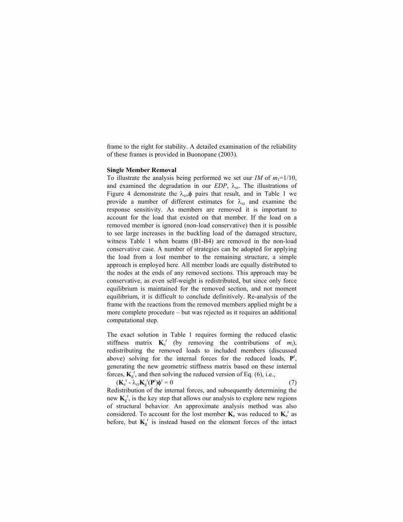
frame to the right for stability. A detailed examination of the reliability of these frames is provided in Buonopane (2003).

Single Member Removal To illustrate the analysis being performed we set our IM of m1=1/10, and examined the degradation in our EDP, λcr. The illustrations of Figure 4 demonstrate the λcr,φ pairs that result, and in Table 1 we provide a number of different estimates for λcr and examine the response sensitivity. As members are removed it is important to account for the load that existed on that member. If the load on a removed member is ignored (non-load conservative) then it is possible to see large increases in the buckling load of the damaged structure, witness Table 1 when beams (B1-B4) are removed in the non-load conservative case. A number of strategies can be adopted for applying the load from a lost member to the remaining structure, a simple approach is employed here. All member loads are equally distributed to the nodes at the ends of any removed sections. This approach may be conservative, as even self-weight is redistributed, but since only force equilibrium is maintained for the removed section, and not moment equilibrium, it is difficult to conclude definitively. Re-analysis of the frame with the reactions from the removed members applied might be a more complete procedure – but was rejected as it requires an additional computational step.

The exact solution in Table 1 requires forming the reduced elastic stiffness matrix Ke

r (by removing the contributions of mi), redistributing the removed loads to included members (discussed above) solving for the internal forces for the reduced loads, Pr, generating the new geometric stiffness matrix based on these internal forces, Kg

r, and then solving the reduced version of Eq. (6), i.e., (Ke

r - λcrKgr(Pr)φr = 0 (7)

Redistribution of the internal forces, and subsequently determining the new Kg

r, is the key step that allows our analysis to explore new regions of structural behavior. An approximate analysis method was also considered. To account for the lost member Ke was reduced to Ke

r as before, but Kg

r is instead based on the element forces of the intact

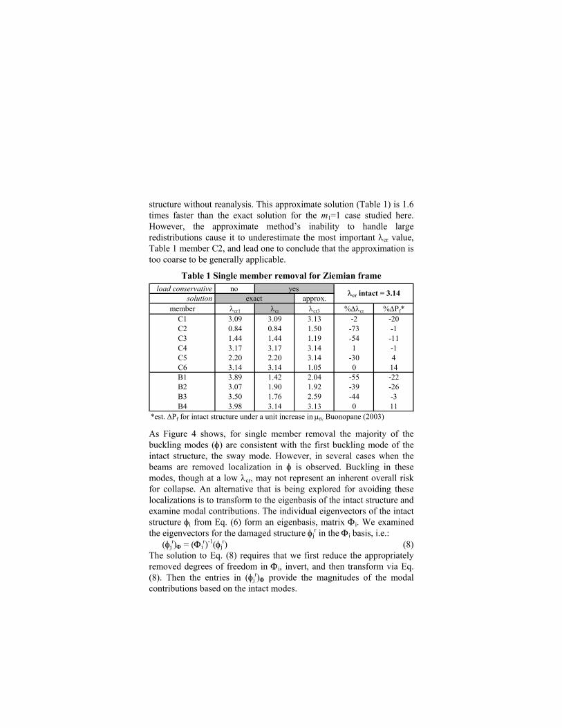
structure without reanalysis. This approximate solution (Table 1) is 1.6 times faster than the exact solution for the m1=1 case studied here. However, the approximate method’s inability to handle large redistributions cause it to underestimate the most important λcr value, Table 1 member C2, and lead one to conclude that the approximation is too coarse to be generally applicable.

Table 1 Single member removal for Ziemian frame load conservative no yes

solution exact approx.member λcr1 λcr λcr3 %∆λcr %∆Pf*

C1 3.09 3.09 3.13 -2 -20C2 0.84 0.84 1.50 -73 -1C3 1.44 1.44 1.19 -54 -11C4 3.17 3.17 3.14 1 -1C5 2.20 2.20 3.14 -30 4C6 3.14 3.14 1.05 0 14B1 3.89 1.42 2.04 -55 -22B2 3.07 1.90 1.92 -39 -26B3 3.50 1.76 2.59 -44 -3B4 3.98 3.14 3.13 0 11

*est. ∆Pf for intact structure under a unit increase in µfy Buonopane (2003)

λcr intact = 3.14

As Figure 4 shows, for single member removal the majority of the buckling modes (φ) are consistent with the first buckling mode of the intact structure, the sway mode. However, in several cases when the beams are removed localization in φ is observed. Buckling in these modes, though at a low λcr, may not represent an inherent overall risk for collapse. An alternative that is being explored for avoiding these localizations is to transform to the eigenbasis of the intact structure and examine modal contributions. The individual eigenvectors of the intact structure φi from Eq. (6) form an eigenbasis, matrix Φi. We examined the eigenvectors for the damaged structure φj

r in the Φi basis, i.e.: (φj

r)Φ = (Φir)-1(φj

r) (8) The solution to Eq. (8) requires that we first reduce the appropriately removed degrees of freedom in Φi, invert, and then transform via Eq. (8). Then the entries in (φj

r)Φ provide the magnitudes of the modal contributions based on the intact modes.

λcr

=3.09 λcr

=3.17

λcr

=0.839 λcr

=2.21

λcr

=1.44 λcr

=3.13

λcr

=1.76 λcr

=3.14

λcr

=1.42 λcr

=1.9

Figure 4 First buckling load and mode of example 1 with one member removed, λcr for intact structure is a sway mode at 3.14

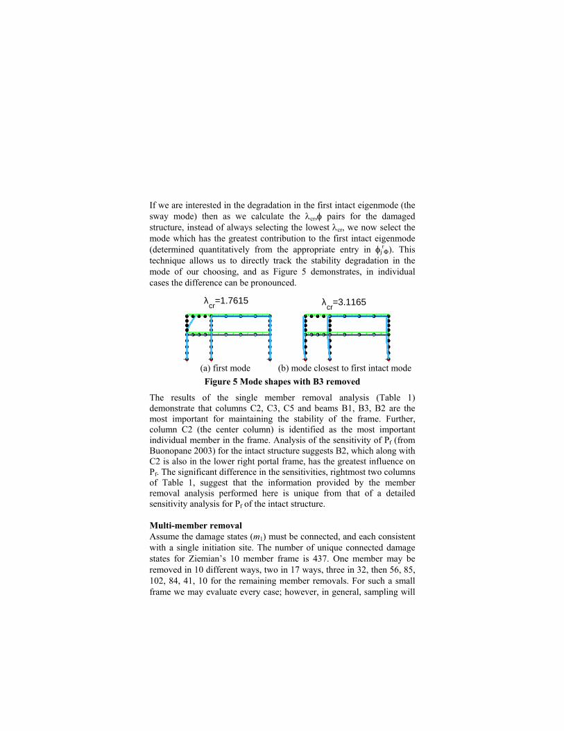
If we are interested in the degradation in the first intact eigenmode (the sway mode) then as we calculate the λcr,φ pairs for the damaged structure, instead of always selecting the lowest λcr, we now select the mode which has the greatest contribution to the first intact eigenmode (determined quantitatively from the appropriate entry in φj

rΦ). This

technique allows us to directly track the stability degradation in the mode of our choosing, and as Figure 5 demonstrates, in individual cases the difference can be pronounced.

λcr

=1.7615 λcr

=3.1165

(a) first mode (b) mode closest to first intact mode Figure 5 Mode shapes with B3 removed

The results of the single member removal analysis (Table 1) demonstrate that columns C2, C3, C5 and beams B1, B3, B2 are the most important for maintaining the stability of the frame. Further, column C2 (the center column) is identified as the most important individual member in the frame. Analysis of the sensitivity of Pf (from Buonopane 2003) for the intact structure suggests B2, which along with C2 is also in the lower right portal frame, has the greatest influence on Pf. The significant difference in the sensitivities, rightmost two columns of Table 1, suggest that the information provided by the member removal analysis performed here is unique from that of a detailed sensitivity analysis for Pf of the intact structure.

Multi-member removal Assume the damage states (m1) must be connected, and each consistent with a single initiation site. The number of unique connected damage states for Ziemian’s 10 member frame is 437. One member may be removed in 10 different ways, two in 17 ways, three in 32, then 56, 85, 102, 84, 41, 10 for the remaining member removals. For such a small frame we may evaluate every case; however, in general, sampling will

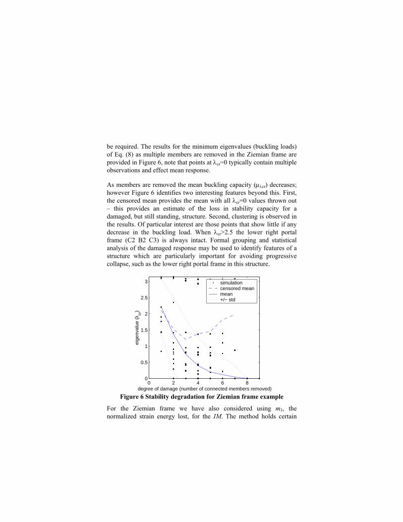
be required. The results for the minimum eigenvalues (buckling loads) of Eq. (8) as multiple members are removed in the Ziemian frame are provided in Figure 6, note that points at λcr=0 typically contain multiple observations and effect mean response.

As members are removed the mean buckling capacity (µλcr) decreases; however Figure 6 identifies two interesting features beyond this. First, the censored mean provides the mean with all λcr=0 values thrown out – this provides an estimate of the loss in stability capacity for a damaged, but still standing, structure. Second, clustering is observed in the results. Of particular interest are those points that show little if any decrease in the buckling load. When λcr>2.5 the lower right portal frame (C2 B2 C3) is always intact. Formal grouping and statistical analysis of the damaged response may be used to identify features of a structure which are particularly important for avoiding progressive collapse, such as the lower right portal frame in this structure.

0 2 4 6 8

0

0.5

1

1.5

2

2.5

3

degree of damage (number of connected members removed)

eige

nval

ue (λ

cr)

simulationcensored meanmean+/− std

Figure 6 Stability degradation for Ziemian frame example

For the Ziemian frame we have also considered using m3, the normalized strain energy lost, for the IM. The method holds certain

advantages as over 90% of the strain energy is contained in the stiffer right-side bay of the frame, and sensitivity to loss of these members is greater. However, it has disadvantages as well, in particular, bending strain energy dominates and the beams are given greater importance than the columns. Either m1 (normalized number of members removed) or m3 may be determined from the same analysis, so at this point they remain computationally interchangeable and the analysis presented here continues to focus on the simpler m1.

Fragility We may use the results of Figure 6 to provide the fragility response of our example frame, Figure 7. This fragility would then be convolved with a probabilistic measure of IM to solve Eq. (2) for Pf. Curves for P(λcr<1) and P(λcr=0) are both provided. If the applied reference loads are the service loads then λcr<1 implies elastic buckling may occur under the service loads in the damaged state.

The solutions where λcr = 0 are of particular interest. For one, finding λcr = 0 is cheap to calculate, only the condition number of Ke

r is needed to determine that the structure is unstable. Second, λcr = 0 implies that the damage will evolve to the next higher level, i.e., if n1 = 2 and λcr=0 then the particular frame would progress to n1=3 with no additional load; whether or not n1 = 3 would cause further progression would depend on exactly which 3 members had been lost. This suggests an estimate for the probability of progressive collapse given the damage level. Since the estimate only includes λcr = 0 values, it is a lower bound estimate of Pf, but cheap to calculate. Specifically, define the probability that λcr=0 at state nd as Pd. The probability that progressive collapse, Pc, will occur given nd=ni and a total of k members

( ) ∏+=

==k

iddiid PPnnP

1c (9)

Results of Eq. (9) are also provided in Figure 7.

0 2 4 6 8 100

0.1

0.2

0.3

0.4

0.5

0.6

0.7

0.8

0.9

1

degree of damage (number of connected members removed)

buck

ling

load

pro

babi

litie

s

P(λcr

<1)P(λ

cr=0)

Pc|(n

d=n

i)

Figure 7 Fragility of Ziemian frame

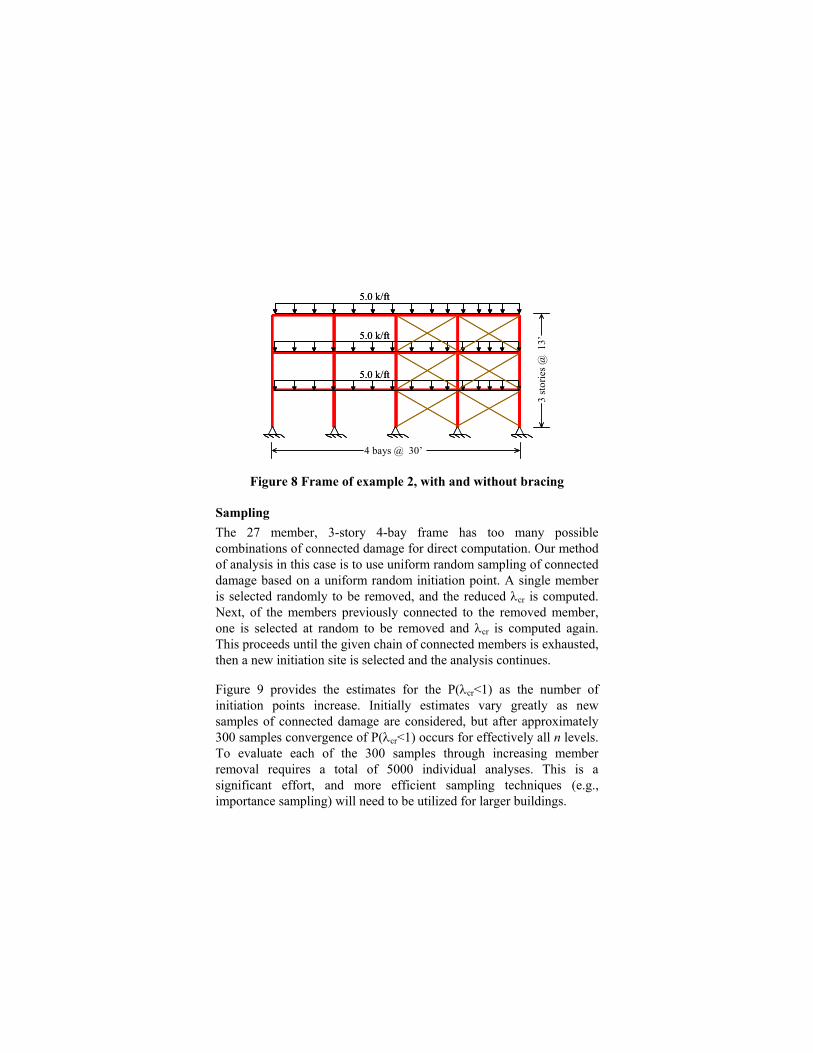
EXAMPLE 2: FRAME WITH AND WITHOUT BRACING The second example selected for study is a 3-story 4-bay moment frame. The basic geometry and assumed service load for the frame is shown in Figure 8. The member sizes are selected for demonstrative purposes only and employ lighter than normal sections (note the relatively low λcr values in Figure 10). Analysis considering the stability degradation of the moment frame under increasing damage is performed both with and without the cross-bracing. The cross-bracing is sized such that a simple braced frame would have the same sway buckling load as the full moment frame without the bracing. Consideration of the bracing is an attempt to examine the influence of a redundant secondary system on the degradation of the stability.

3 st

orie

s @ 1

3’

5.0 k/ft

5.0 k/ft

5.0 k/ft

4 bays @ 30’

3 st

orie

s @ 1

3’

5.0 k/ft

5.0 k/ft

5.0 k/ft

4 bays @ 30’

Figure 8 Frame of example 2, with and without bracing

Sampling The 27 member, 3-story 4-bay frame has too many possible combinations of connected damage for direct computation. Our method of analysis in this case is to use uniform random sampling of connected damage based on a uniform random initiation point. A single member is selected randomly to be removed, and the reduced λcr is computed. Next, of the members previously connected to the removed member, one is selected at random to be removed and λcr is computed again. This proceeds until the given chain of connected members is exhausted, then a new initiation site is selected and the analysis continues.

Figure 9 provides the estimates for the P(λcr<1) as the number of initiation points increase. Initially estimates vary greatly as new samples of connected damage are considered, but after approximately 300 samples convergence of P(λcr<1) occurs for effectively all n levels. To evaluate each of the 300 samples through increasing member removal requires a total of 5000 individual analyses. This is a significant effort, and more efficient sampling techniques (e.g., importance sampling) will need to be utilized for larger buildings.

100 200 300 400 500 6000

0.2

0.4

0.6

0.8

1

No. of Samples

Lim

it S

tate

Pro

babi

lity

(P[λ

cr <

1]) n = 5

n = 4

n = 3

n = 2

Figure 9 Sampling effort and convergence for example 2

0 5 10 15

0

0.5

1

1.5

2

2.5

3

3.5

degree of damage (no. of connected members removed)

eige

nval

ue (λ

cr)

simulationmeansimulation with x−bracingsmean with x−bracings

Figure 10 Stability degradation for example 2

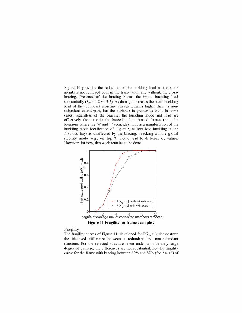
Figure 10 provides the reduction in the buckling load as the same members are removed both in the frame with, and without, the cross-bracing. Presence of the bracing boosts the initial buckling load substantially (λcr ~ 1.8 vs. 3.2). As damage increases the mean buckling load of the redundant structure always remains higher than its non-redundant counterpart, but the variance is greater as well. In some cases, regardless of the bracing, the buckling mode and load are effectively the same in the braced and un-braced frames (note the locations where the ‘o’ and ‘·’ coincide). This is a manifestation of the buckling mode localization of Figure 5, as localized buckling in the first two bays is unaffected by the bracing. Tracking a more global stability mode (e.g., via Eq. 8) would lead to different λcr values. However, for now, this work remains to be done.

0 2 4 6 8 10

0

0.2

0.4

0.6

0.8

1

degree of damage (no. of connected members removed)

limit

stat

e pr

obab

ility

(p[

λ cr <

1])

P[λcr

< 1] without x−bracesP[λ

cr < 1] with x−braces

Figure 11 Fragility for frame example 2

Fragility The fragility curves of Figure 11, developed for P(λcr<1), demonstrate the idealized difference between a redundant and non-redundant structure. For the selected structure, even under a moderately large degree of damage, the differences are not substantial. For the fragility curve for the frame with bracing between 63% and 87% (for 2<n<6) of

the λcr<1 values are actually λcr~0. These low λcr values occur due to buckling mode localization in the first two bays and are the same for the frame with and without braces. However, as the number of damaged members increases the redundant system provides benefits. If we assume a normal distribution for the intensity measure with mean of 2 removed members and variance of 2 removed members, i.e., IM = N(2,2), then Pf is 28% for the non-redundant frame and 23% for the redundant frame. For higher IM distribution, IM=N(5,2) Pf is 66% and 56% respectively. Though Pf decreases, whether or not the redundant system is worth the expense remains an open question, but could be evaluated by associating a cost with v(DV) of Eq. (1) instead of Pf.

DISCUSSION To provide the Pf in an unforeseen hazard, solution to Eq. (2) is needed. At this point the most problematic unknowns are the distributions of the intensities (e.g., IM=N(2,2)). What intensities match our desired/experienced levels of intensity? From a frequentist standpoint, with so little data available, this may sound impossible to do. However, even in conventional design, Pf is only useful for comparative purposes and does not strictly provide a prediction comparable to observed failure rates. We intend to develop our performance levels based on examinations of existing building systems, both bad and good, and subsequent categorization.

Since we are generally interested in structural collapse, rather than loss of stability in one portion of the structure, efficiently avoiding the mode localization of Figure 5(a) remains a distinct challenge. Use of the intact eigenbasis shows promise, but ignoring the minimum eigenmode in favor of one closer to the anticipated mode has its own hazards. The advantage of using the stability analysis is that λcr provides a single scalar measure of the response, if multiple modes and situations have to be tracked then this advantage may be lost.

The role redundancy plays in the stability response is not fully brought to light in example 2. Further work on redundant systems with multiple load paths is needed. Simple robust measures of redundancy, such as

the mean number of members that can be removed before the first λcr=0 is encountered, need further examination for a wider class of structures. A great deal of work on redundancy, for example that of Frangopol and his colleagues, provides insights not yet put into practice here.

Other essential future work includes the examination of additional intensity measures and demand parameters. Further, more formal methods for understanding the sensitivity of damaged structures are needed. For example, the probability and sensitivity each member has on the P(λcr<1) may be crucial information for identifying individual members that are highly influential to the system response.

The primary challenge for completing the analysis with large-scale three-dimensional structures is computational efficiency. Recent work by Kirsch (2003) provides alternatives, but more work clearly remains. Better sampling may provide the most efficient route, particularly if assessing P(λcr<x) is of greatest interest as opposed to the entire response. The direct use of the condition number under increasing intensity of damage, for a coarse estimate of stability, may provide an efficient check. This idea will be pursued for other structural systems.

CONCLUSIONS To explore system behavior and understand building response in extreme events we need to augment our load case based, foreseen event, environmental hazard analysis with damage based, unforeseen event, hazard analysis. It is suggested that the existing performance-based seismic design framework can be modified for unforeseen events. Employing an intensity measure based on removing members, and a demand parameter based on the degradation of the first buckling load is shown to provide a method for examining structures in unforeseen events. Load conservative, exact solutions are necessary, and computational demands grow quickly for this form of re-analysis. Comparing sensitivity of the intact structure’s Pf and sensitivity of the damaged structure’s stability (λcr) leads us to conclude that the new structural systems that result when discontinuities are introduced by member removal bring new failure paths and modes of behavior to

light. Tracking the degradation of buckling load in a given mode shape, and tracking the minimum buckling load regardless of mode shape are both possible, but give different results. Fragility curves developed based on degradation in the first buckling load (namely P(λcr<1) provide useful and reasonable tools for assessing fragility to severe unforeseen hazards. Progressive collapse may be cheaply estimated using the condition number of a damaged frame’s stiffness matrix. Even on relatively small two-dimensional structures the large number of possible damage combinations require sampling. Degradation of the first stability eigenmode, as members are removed, provides a method for examining fragility of structures under extreme unforeseen events.

ACKNOWLEDGMENTS The research for this paper was partially sponsored by a grant from the National Science Foundation (NSF-DMII-0228246).

REFERENCES AISC (2001). Manual of Steel Construction: Load and Resistance

Factor Design 3rd Ed. American Inst. of Steel Const. Chicago, IL. ASCE 7 (1998). Minimum Design Loads for Buildings and Other

Structures. ASCE. Buonopane, S.G. (2003). Reliability and Bayesian Approaches to the

Probabilistic Performance Based Design of Structures. Ph.D. Dissertation, Johns Hopkins University, Baltimore, MD.

Cornell. C.A. Jalayer, F., Hamburger, R.O. (2002). “Probabilistic Basis for the 2000 SAC FEMA Steel Moment Frame Guidelines.” ASCE. J. of Structural Engineering. 128 (4) 526-533.

Deierlein, G.G. (2002). “Overview of the PEER Performance-Based Earthquake Engineering Methodology.” PEER Center Annual Mtg.

Kirsch, U. (2003). “Design-Oriented Analysis of Structures – Unified Approach.” ASCE. J. of Structural Engineering. 129 (3) 264-272.

Yun, S., Hamburger, R.O., Cornell, C.A., Foutch, D.A. (2002). “Seismic Performance Evaluation for Steel Moment Frames.” ASCE. J. of Structural Engineering. 128 (4) 534-545.

Ziemian, R.D. McGuire, W. & Deierlein, G.G. (1992). “Inelastic limit states design. part I: planar frame studies.” J. of Structural Engineering, 118 (9) 2532-2549.

KEYWORD INDEX stability degradation 2,7,11,12,14,16 redundancy/redundant 1,3,14,17,19 damaged structure(s) 1,6-9,11,19,20 unforeseen hazard(s)/event(s) 1-5,18-20 progressive collapse 1,12,13,20 buckling 1,5,6,8,9,12-14,16,17,20 REFERENCE INDEX AISC (2001) 2 ASCE 7 (1998) 2 Buonopane (2003) 9 Cornell et al. (2002) 4 Deierlein (2002) 2 Kirsch, U. (2003) 19 Yun et al. (2002) 4 Ziemian et al. (1992) 7