Stability Analysis of Uzawa-Lucas Endogenous Growth Modelkuwpaper/2009Papers/201304.pdf ·...

1

Stability Analysis of Uzawa-Lucas Endogenous Growth Model

William A. Barnett*

University of Kansas, Lawrence

and Center for Financial Stability, NY City

and

Taniya Ghosh

Indira Gandhi Institute of Development Research (IGIDR), Reserve Bank of India, Mumbai

May 20, 2013

Abstract:

This paper analyzes, within its feasible parameter space, the dynamics of the Uzawa-Lucas endogenous growth

model. The model is solved from a centralized social planner perspective as well as in the model’s decentralized

market economy form. We examine the stability properties of both versions of the model and locate Hopf and

transcritical bifurcation boundaries. In an extended analysis, we investigate the existence of Andronov-Hopf

bifurcation, branch point bifurcation, limit point cycle bifurcation, and period doubling bifurcations. While these all

are local bifurcations, the presence of global bifurcation is confirmed as well. We find evidence that the model could

produce chaotic dynamics, but our analysis cannot confirm that conjecture.

It is important to recognize that bifurcation boundaries do not necessarily separate stable from unstable solution

domains. Bifurcation boundaries can separate one kind of unstable dynamics domain from another kind of unstable

dynamics domain, or one kind of stable dynamics domain from another kind (called soft bifurcation), such as

bifurcation from monotonic stability to damped periodic stability or from damped periodic to damped multiperiodic

stability. There are not only an infinite number of kinds of unstable dynamics, some very close to stability in

appearance, but also an infinite number of kinds of stable dynamics. Hence subjective prior views on whether the

economy is or is not stable provide little guidance without mathematical analysis of model dynamics.

When a bifurcation boundary crosses the parameter estimates’ confidence region, robustness of dynamical

inferences from policy simulations are compromised, when conducted, in the usual manner, only at the parameters’

point estimates.

Keywords: bifurcation, endogenous growth, Lucas-Uzawa model, Hopf, inference robustness, dynamics, stability.

*Corresponding author: William A. Barnett, email: [email protected], tel: 1-785-832-1342,

fax: 1-785-832-1527.

2

1. Introduction

The Uzawa-Lucas model (Uzawa (1965) and Lucas (1988)), upon which many others have

been built, is among the most important endogenous growth models. The model has two sectors:

the human capital production sector and the physical capital production sector producing human

capital and physical capital, respectively. Individuals have the same level of work qualification

and expertise (H). They allocate some of their time to producing final goods and dedicate the

remaining time to training and studying.

The social planner solution for the Uzawa-Lucas model is saddle path stable, but the

representative agent’s equilibrium can be indeterminate, as shown by Benhabib and Perli (1994).

As a result of the presence of externalities in human capital, the market solution is different from

the social planner solution. The externality creates a distinction between return on capital, as

perceived by the representative agent, to that perceived by a social planner.

We solve for the steady states and provide a detailed bifurcation analysis of the model. The

task of this paper is to examine whether the dynamics of the model change within the feasible

parameter space of the model. A system undergoes a bifurcation, if a small, smooth change in a

parameter produces a sudden qualitative or topological change in the nature of singular points and

trajectories of the system. The presence of bifurcation damages the inference robustness of the

dynamics, when inferences are based on point estimates of the model. Hence, knowing the

stability boundaries within the feasible region of the parameter space, especially near the point

estimates, can lead to more robust dynamical inferences and more reliable policy conclusions.

Using Mathematica, we locate transcritical and Hopf bifurcation boundaries in two-

dimension and three-dimension diagrams. The numerical continuation package, Matcont, is used

to analyze further the stability properties of the limit cycles generated by Hopf bifurcations and

the presence of other kinds of bifurcations. We show the existence of Hopf, branch-point, limit-

point-of-cycles, and period-doubling bifurcations within the feasible parameters set of the

model’s parameter space. While these are all local bifurcations, presence of global bifurcation is

also confirmed. There is some evidence of the possibility of chaotic dynamics through the

detected series of period-doubling bifurcations, known to converge to chaos. Some of these

results have not previously been demonstrated in the literature on endogenous growth models.

3

Benhabib and Perli (1994) analyzed the stability property of the long-run equilibrium in the

Lucas (1988) model. Arnold (2000a,b) analyzed the stability of equilibrium in the Romer (1990)

model. Arnold (2006) has done the same for the Jones (1995) model. Mondal (2008) examined

the dynamics of the Grossman-Helpman (1991b) model of endogenous product cycles. The

results derived in those papers provide important insights to researchers considering different

policies. But, as in the Benhabib and Perli (1994) paper, a detailed bifurcation analysis has not

been provided so far for many of these popular endogenous growth models. The current paper

aims to fill this gap for the Uzawa-Lucas model.

As pointed out by Banerjee et al (2011): “Just as it is important to know for what parameter

values a system is stable or unstable, it is equally important to know the nature of stability (e.g.

monotonic convergence, damped single periodic convergence, or damped multi-periodic

convergence) or instability (periodic, multi-periodic, or chaotic).” Barnett and his coauthors have

made significant contribution in this area. Barnett and He (1999, 2002) examined the dynamics of

the Bergstrom-Wymer continuous-time dynamic macroeconometric model of the UK economy.

Both transcritical bifurcation boundaries and the Hopf bifurcation boundaries for the model were

found. Barnett and He (2008) have found singularity bifurcation boundaries within the parameter

space for the Leeper and Sims (1994) model. Barnett and Duzhak (2010) found Hopf and period

doubling bifurcations in a New Keynesian model. More recently, Banerjee et al (2011) examined

the possibility of cyclical behavior in the Marshallian Macroeconomic Model and Barnett and

Eryilmaz (2013a,b) have found bifurcation in open economy models.

2. The Uzawa-Lucas Model

The production function in the physical sector is defined as follows:

,

where Y is output, A is constant technology level, K is physical capital, is the share of physical

capital, L is labor, and h is human capital per person. In addition, and are the fraction of

labor time devoted to producing output and human capital, respectively, where .

Observe that is the quantity of labor, measured in efficiency units, employed to produce

output, and

measures the externality associated with average human capital of the work

4

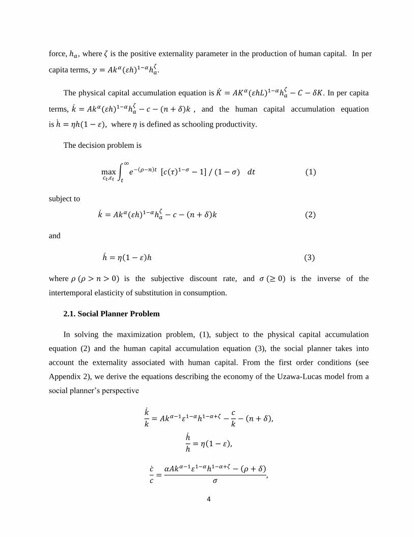
force, , where is the positive externality parameter in the production of human capital. In per

capita terms, .

The physical capital accumulation equation is . In per capita

terms, , and the human capital accumulation equation

is , where is defined as schooling productivity.

The decision problem is

∫

[ ]

subject to

and

where is the subjective discount rate, and is the inverse of the

intertemporal elasticity of substitution in consumption.

2.1. Social Planner Problem

In solving the maximization problem, (1), subject to the physical capital accumulation

equation (2) and the human capital accumulation equation (3), the social planner takes into

account the externality associated with human capital. From the first order conditions (see

Appendix 2), we derive the equations describing the economy of the Uzawa-Lucas model from a

social planner’s perspective

5

Taking logarithms of m and g and differentiating

with respect to time, equations (4) and (5) define the dynamics of Uzawa-Lucas model

(

)

(

)

The steady state is given by and derived to be

A unique steady state exists, if

.

In addition, provides the necessary and sufficient for the transversality condition to hold for the

consumer’s utility maximization problem (see Appendix 1). Following the footsteps of Barro and

Sala-i-Martín (2003) and Mattana (2004), it can be shown that social planner solution is saddle

path stable. We linearize around the steady state, , to analyze the local stability

properties of the system defined by equations (4) and (5). The result is

6

[ ]

[

|

|

|

| ]

⏟

[

]

where

[

(

) ]

As hence saddle path stable.

2.2. Representative Agent Problem

From the first order conditions (see Appendix 3) and setting ,we derive the equations

describing the economy of the Uzawa-Lucas model from a decentralized economy’s perspective.

. Taking logarithms of m and g and differentiating with respect to time, the

following three equations define the dynamics of Uzawa Lucas model

7

(

)

(

)

The steady state is given by and derived to be

[ ]

[ ]

[ ]

Note that as shown by Benhabib and Perli (1994)

[ ]

A unique steady state exists if

In addition, is the necessary and sufficient for the transversality condition to hold for the

consumer’s utility maximization problem (appendix 1), and is necessary for

We linearize the system (6), (7) and (8) around the steady state, , to acquire

[ ]

[

|

|

|

|

|

|

|

|

| ]

⏟

[

]

8

[

(

)

]

.

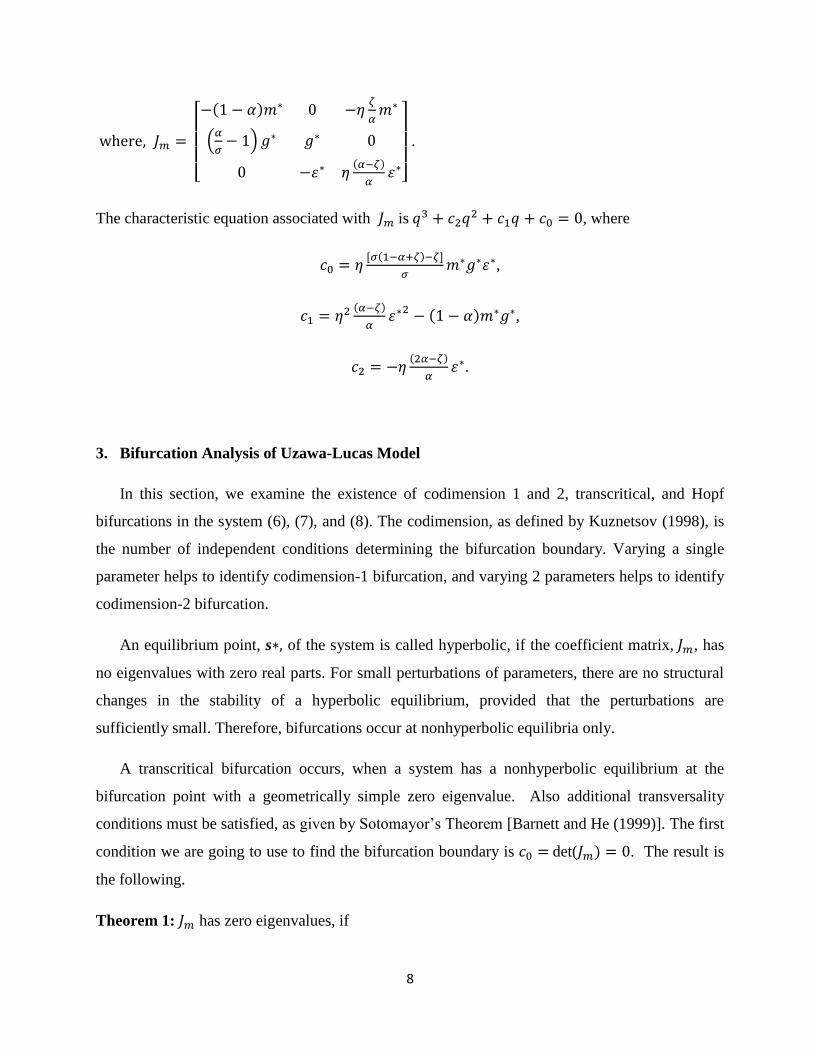
The characteristic equation associated with is , where

[ ]

,

,

.

3. Bifurcation Analysis of Uzawa-Lucas Model

In this section, we examine the existence of codimension 1 and 2, transcritical, and Hopf

bifurcations in the system (6), (7), and (8). The codimension, as defined by Kuznetsov (1998), is

the number of independent conditions determining the bifurcation boundary. Varying a single

parameter helps to identify codimension-1 bifurcation, and varying 2 parameters helps to identify

codimension-2 bifurcation.

An equilibrium point, s , of the system is called hyperbolic, if the coefficient matrix, , has

no eigenvalues with zero real parts. For small perturbations of parameters, there are no structural

changes in the stability of a hyperbolic equilibrium, provided that the perturbations are

sufficiently small. Therefore, bifurcations occur at nonhyperbolic equilibria only.

A transcritical bifurcation occurs, when a system has a nonhyperbolic equilibrium at the

bifurcation point with a geometrically simple zero eigenvalue. Also additional transversality

conditions must be satisfied, as given by Sotomayor’s Theorem [Barnett and He (1999)]. The first

condition we are going to use to find the bifurcation boundary is det( . The result is

the following.

Theorem 1: has zero eigenvalues, if

9

[ ]

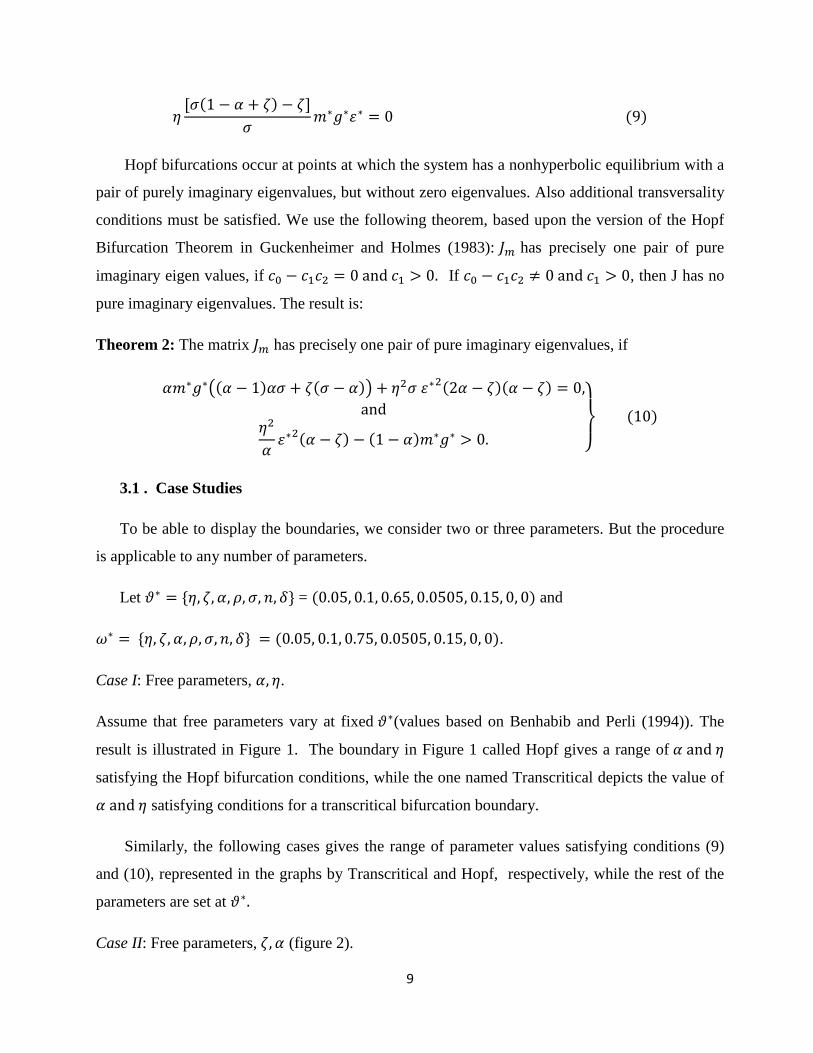
Hopf bifurcations occur at points at which the system has a nonhyperbolic equilibrium with a

pair of purely imaginary eigenvalues, but without zero eigenvalues. Also additional transversality

conditions must be satisfied. We use the following theorem, based upon the version of the Hopf

Bifurcation Theorem in Guckenheimer and Holmes (1983): has precisely one pair of pure

imaginary eigen values, if If , then J has no

pure imaginary eigenvalues. The result is:

Theorem 2: The matrix has precisely one pair of pure imaginary eigenvalues, if

( )

}

3.1 . Case Studies

To be able to display the boundaries, we consider two or three parameters. But the procedure

is applicable to any number of parameters.

Let = and

.

Case I: Free parameters, .

Assume that free parameters vary at fixed (values based on Benhabib and Perli (1994)). The

result is illustrated in Figure 1. The boundary in Figure 1 called Hopf gives a range of

satisfying the Hopf bifurcation conditions, while the one named Transcritical depicts the value of

satisfying conditions for a transcritical bifurcation boundary.

Similarly, the following cases gives the range of parameter values satisfying conditions (9)

and (10), represented in the graphs by Transcritical and Hopf, respectively, while the rest of the

parameters are set at

Case II: Free parameters, (figure 2).

10

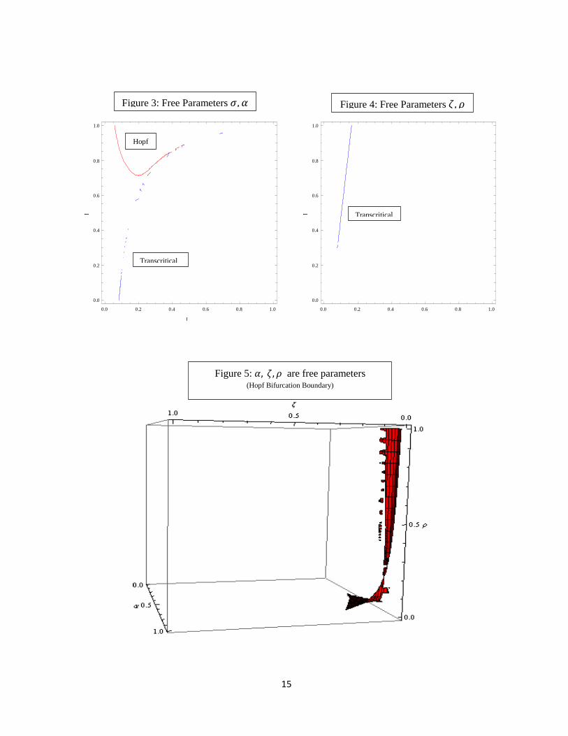
Case III: Free parameters, (figure 3).

Case IV: Free parameters, (figure 4). Notice that for case IV, we do not have a Hopf

bifurcation boundary.

We now add another parameter as a free parameter and continue with the analysis. The

following cases give the range of parameter values satisfying conditions (9) or (10), represented

in the graphs (5)-(9), while the rest of the parameters are assumed to be at

Case V: Free parameters, (figure 5).

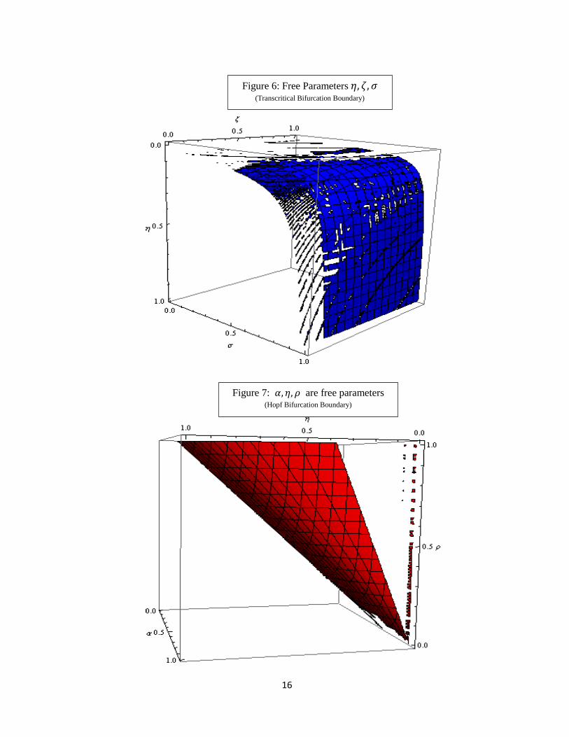
Case VI: Free parameters, (figure 6).

Case VII: Free parameters, (figure 7). Notice that for case IV, we do not have a Hopf

bifurcation boundary.

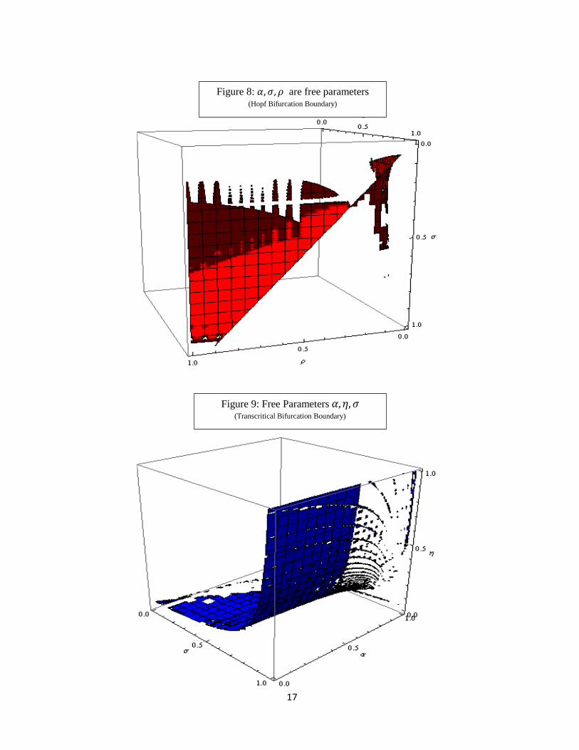
Case VIII: Free parameters, (figure 8).

Case IX: Free parameters, (figure 9).

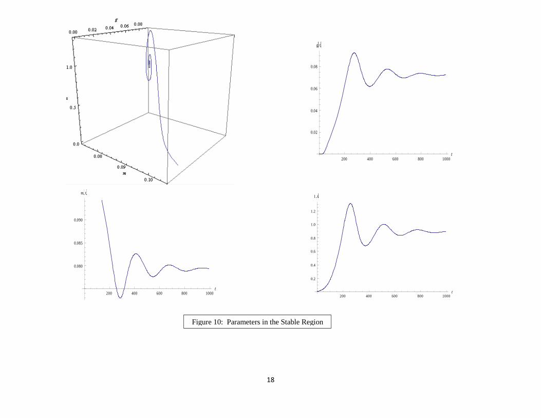
The following is an approach to exploring cyclical behavior in the model. Suppose the

externality parameter increases. This causes the savings rate to increase. This is because when

consumers are willing to cut current consumption in exchange for higher future consumption; that

is, when intertemporal elasticity of substitution for consumption is high ( is low), people start

saving more. Hence there is a movement of labor from output production to human capital

production. Human capital begins increasing. This implies faster accumulation of physical capital,

if sufficient externality to human capital in production of physical capital is present. If people care

about the future more (subjective discount rate is lower), consumption starts rising gradually

with faster capital accumulation, leading to greater consumption-goods production in the future.

This will eventually lead to a decline in savings rate. Two opposing effects come into play when

savings rate is different from the equilibrium rate, causing a cyclical convergence to equilibrium.

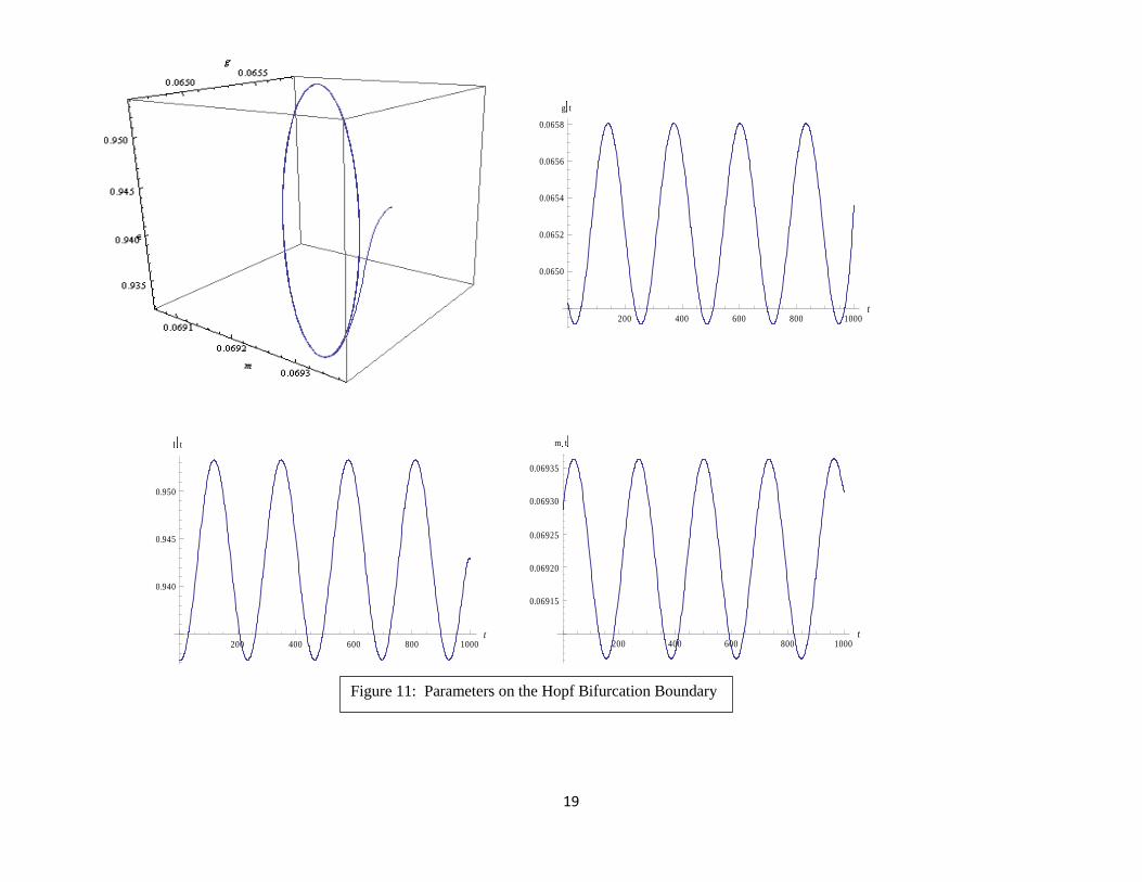
Hence, interaction between different parameters can cause cyclical convergence to equilibrium

(figure 10) or may cause instability; and for some parameter values we may have convergence to

cycles (figure 11).

11

Using the numerical continuation package Matcont, we further investigate the stability

properties of cycles generated by different combinations of parameters. While some of the limit

cycles generated by Andronov-Hopf bifurcation are stable (supercritical bifurcation), there could

be some unstable limit cycles (subcritical bifurcation) created as well. When Hopf bifurcations are

generated, Table 1 reports the values of the share of capital , externality in production of

human capital , and the inverse of intertemporal elasticity of substitution in consumption .

A positive value of the first Lyapunov coefficient indicates creation of subcritical Hopf

bifurcation. Thus for each of the cases reported in Table 1, an unstable limit cycle (periodic orbit)

bifurcates from the equilibrium. All of these cases also produce branch points

(pitchfork/transcritical bifurcations).

Continuation of limit cycles from the Hopf point, when is the free parameter, gives rise to

limit point (Fold/ Saddle Node) bifurcation of cycles. From the family of limit cycles bifurcating

from the Hopf point, limit point cycle (LPC) is a fold bifurcation, where two limit cycles with

different periods are present near the LPC point at = 0.738.

Continuing computation further from a Hopf point gives rise to a series of period doubling

(flip) bifurcations. Period doubling bifurcation is defined as a situation in which a new limit cycle

emerges from an existing limit cycle, and the period of the new limit cycle is twice that of the old

one. The first period doubling bifurcation, at = 0.7132369, has positive normal form

coefficients, indicating existence of unstable double-period cycles. The rest of the period

doubling bifurcations have negative normal-form coefficients, giving rise to stable double-period

cycles.

The period of the cycle rapidly increases for very small perturbation in parameter , as is

evident in figure 12(C). The limit cycle approaches a global homoclinic orbit. A homoclinic orbit

is a dynamical system trajectory, which joins a saddle equilibrium point to itself. In other words, a

homoclinic orbit lies in the intersection of equilibrium’s stable manifold and unstable manifold.

There exists the possibility of reaching chaotic dynamics in the decentralized version of Uzawa-

Lucas model through a series of period doubling bifurcations.

For the cases in which and are free parameters, we carry out the continuation of limit

cycle from the first Hopf point. Both cases give rise to limit point cycles with a nonzero normal-

http://en.wikipedia.org/wiki/Dynamical_system

http://en.wikipedia.org/wiki/Stable_manifold

http://en.wikipedia.org/wiki/Unstable_manifold

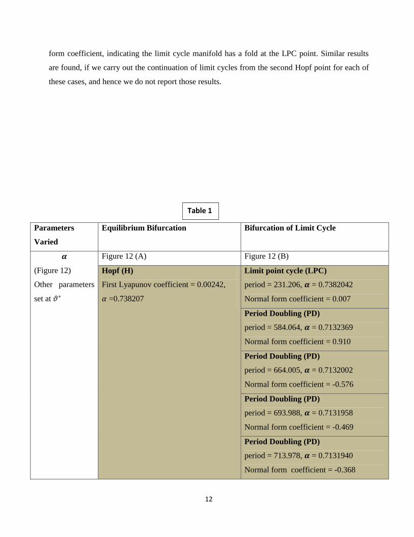
12

form coefficient, indicating the limit cycle manifold has a fold at the LPC point. Similar results

are found, if we carry out the continuation of limit cycles from the second Hopf point for each of

these cases, and hence we do not report those results.

Parameters

Varied

Equilibrium Bifurcation Bifurcation of Limit Cycle

(Figure 12)

Other parameters

set at

Figure 12 (A) Figure 12 (B)

Hopf (H)

First Lyapunov coefficient = 0.00242,

=0.738207

Limit point cycle (LPC)

period = 231.206, = 0.7382042

Normal form coefficient = 0.007

Period Doubling (PD)

period = 584.064, = 0.7132369



period = 664.005, = 0.7132002

Normal form coefficient = -0.576


period = 693.988, = 0.7131958



period = 713.978, = 0.7131940


Table 1

13


period = 725.667, = 0.7131932



period = 784.104, = 0.7131912


Branch Point (BP)

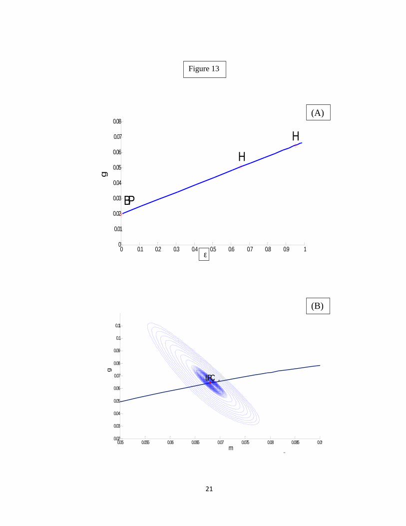
(Figure 13)

Other parameters

set at


Hopf (H)

First Lyapunov coefficient = 0.00250,

=0.107315


period = 215.751, = 0.1073147


Hopf (H)

First Lyapunov coefficient = 0.00246

=0.052623

Branch Point (BP)

(Figure 14)

Other parameters

set at


Hopf (H)


=0.278571


period = 213.83, = 0.1394026


Hopf (H)


=0.139394

Branch Point (BP)

14

0.0 0.2 0.4 0.6 0.8 1.0

0.0

0.2

0.4

0.6

0.8

1.0

0.0 0.2 0.4 0.6 0.8 1.0

0.0

0.2

0.4

0.6

0.8

1.0

Figure 2: Free Parameters 𝜁 𝛼

Figure 1: Free Parameters 𝛼 𝜂

Hopf

Transcritical

Hopf

Transcritical

15

0.0 0.2 0.4 0.6 0.8 1.0

0.0

0.2

0.4

0.6

0.8

1.0 T p qu

Figure 4: Free Parameters 𝜁 𝜌 Figure 3: Free Parameters 𝜎 𝛼

0.0 0.2 0.4 0.6 0.8 1.0

0.0

0.2

0.4

0.6

0.8

1.0

Figure 5: 𝛼 𝜁 𝜌 are free parameters (Hopf Bifurcation Boundary)

Transcritical

Transcritical

Hopf

16

Figure 6: Free Parameters 𝜂 𝜁 𝜎 (Transcritical Bifurcation Boundary)

𝜂 𝜁 𝜎

Figure 7: 𝛼 𝜂 𝜌 are free parameters (Hopf Bifurcation Boundary)

17

Figure 8: 𝛼 𝜎 𝜌 are free parameters (Hopf Bifurcation Boundary)

Figure 9: Free Parameters 𝛼 𝜂 𝜎 (Transcritical Bifurcation Boundary)

18

200 400 600 800 1000t

0.02

0.04

0.06

0.08

g t

200 400 600 800 1000t

0.080

0.085

0.090

m t

200 400 600 800 1000t

0.2

0.4

0.6

0.8

1.0

1.2

t

Figure 10: Parameters in the Stable Region

19

200 400 600 800 1000t

0.0650

0.0652

0.0654

0.0656

0.0658

g t

200 400 600 800 1000t

0.940

0.945

0.950

t

200 400 600 800 1000t

0.06915

0.06920

0.06925

0.06930

0.06935

m t

Figure 11: Parameters on the Hopf Bifurcation Boundary

20

0 0.1 0.2 0.3 0.4 0.5 0.6 0.7 0.8 0.9 10

0.02

0.04

0.06

0.08

0.1

0.12

e

g BP H

0.7 0.705 0.71 0.715 0.72 0.725 0.73 0.735 0.74 0.745

250

300

350

400

450

500

550

600

650

700

750

k1

Period

LPC

PD

PD PD

PD PD PD

PD

PD PD PD

0 0.01 0.02 0.03 0.04 0.05 0.06 0.07 0.08 0.09 0.10

0.05

0.1

0.15

0.2

0.25

m

g

LPC

PD

PD

PD

PD

PD

PD

PD

PD

α

(C)

(B)

(A)

Figure 12

Ɛ

21

0 0.1 0.2 0.3 0.4 0.5 0.6 0.7 0.8 0.9 10

0.01

0.02

0.03

0.04

0.05

0.06

0.07

0.08

e

g

H

H

BP

0.05 0.055 0.06 0.065 0.07 0.075 0.08 0.085 0.090.02

0.03

0.04

0.05

0.06

0.07

0.08

0.09

0.1

0.11

m

g

BP

H H

H

H

BP

H BPH LPC

Ɛ

Figure 13

(A)

(B)

22

0.05 0.055 0.06 0.065 0.07 0.075 0.08 0.085 0.09 0.095 0.10

0.02

0.04

0.06

0.08

0.1

m

g

H

BP

H

0 0.01 0.02 0.03 0.04 0.05 0.06 0.07 0.08 0.09 0.10

0.1

0.2

0.3

0.4

0.5

m

g

LPC

(A)

(B)

Figure 14

23

4. Conclusion

This paper provides a detailed stability and bifurcation analysis of the Uzawa-Lucas model.

Transcritical bifurcation and Hopf bifurcation boundaries, corresponding to different combinations

of parameters, are located for the decentralized version of the model. Examination of the stability

properties of the limit cycles generated from various Hopf bifurcations in the model depicts

occurrence of limit point-of-cycles bifurcations and period-doubling bifurcations within the model’s

feasible parameter set. The series of period-doubling bifurcations confirms the presence of global

bifurcation. Period-doubling bifurcations also reveal the possibility of chaotic dynamics, occurring

in the converged limit of the sequence of period doubling. In contrast, the centralized social planner

solution is always saddle path stable, with no possibility of bifurcation within the feasible parameter

set, but with no decentralized informational privacy. Thus the externality of the human capital

parameter plays an important role in determining the dynamics of the decentralized Uzawa-Lucas

model. Our result emphasizes the need for simulations of decentralized macro econometric models

at settings throughout the parameter-estimates’ confidence regions, rather than at the point estimates

alone, since dynamical inferences otherwise can produce oversimplified conclusions subject to

robustness problems.

=====================================================================

Appendix 1:

In the steady state, the constancy of implies

.

Transversality conditions require and , which in turn imply

,

where and are costate variables (appendix 2 and appendix 3)

Appendix 2:

Social Planner Problem:

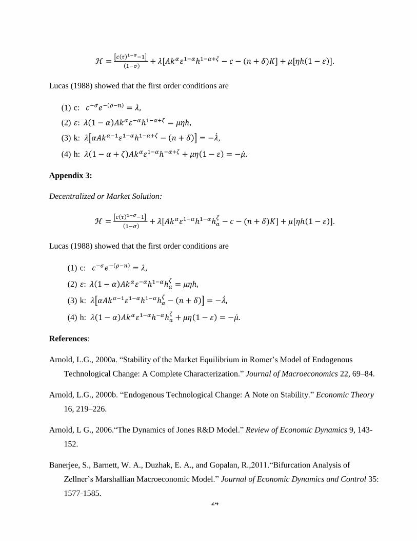
24

[ ]

[ ] [ ].

Lucas (1988) showed that the first order conditions are

(1) c:

(2)

(3) k: [ ]

(4) h:

Appendix 3:

Decentralized or Market Solution:

[ ]

[

] [ ].

Lucas (1988) showed that the first order conditions are

(1) c:

(2)

(3) k: [ ]

(4) h:

References:

Arnold, L.G., 2000a. “Stability of the Market Equilibrium in Romer’s Model of Endogenous

Technological Change: A Complete Characterization.” Journal of Macroeconomics 22, 69–84.

Arnold, L.G., 2000b. “Endogenous Technological Change: A Note on Stability.” Economic Theory

16, 219–226.

Arnold, L G., 2006.“The Dynamics of Jones R&D Model.” Review of Economic Dynamics 9, 143-

152.

Banerjee, S., Barnett, W. A., Duzhak, E. A., and Gopalan, R.,2011.“Bifurcation Analysis of

Zellner’s Marshallian Macroeconomic Model.” Journal of Economic Dynamics and Control 35:

1577-1585.

25

Barnett W.A. and Duzhak, E.A., 2010. “Empirical Assessment of Bifurcation Regions within New

Keynesian Models. “Economic Theory 45, 99-128.

Barnett, W. A. and He, Y., 1999. “Stability Analysis of Continuous-Time Macroeconometric

Systems.” Studies in Nonlinear Dynamics & Econometrics 3, 169-188.

Barnett, W. A. and He, Y., 2002. “Stabilization Policy as Bifurcation Selection: Would Stabilization

Policy Work If the Economy Really Were Unstable?” Macroeconomic Dynamics 6, 713-747

Barnett, W. A. and He, Y., 2008. “Existence of Singularity Bifurcation in an Euler-Equations Model

of the United States Economy: Grandmont Was Right.” Physica A 387, 3817-3825.

Barnett, W. A. and Eryilmaz, U., 2013a. "Hopf Bifurcation in the Clarida, Gali, and Gertler Model."

Economic Modelling 31, 401-404.

Barnett, W. A. and Eryilmaz, U., 2013b. "An Analytical and Numerical Search for Bifurcations in

Open Economy New Keynesian Models." Macroeconomic Dynamics, forthcoming.

Barro, R. J. and Sala-i-Martin, X., 2003, Economic Growth, Second Edition, The MIT Press

Benhabib, J. and Perli, R., 1994, “Uniqueness and Indeterminacy on the Dynamics of Endogenous

Growth.” Journal of Economic Theory 63, 113-142.

Guckenheimer, J. and Holmes, P. , 1983. Nonlinear Oscillations, Dynamical Systems, and

Bifurcations of Vector Fields. New York: Springer-Verlag.

Guckenheimer, J., Myers, M., and Sturmfels, B., 1997. “Computing Hopf Bifurcations, I.” SIAM

Journal on Numerical Analysis 34, 1–21.

Grossman, G. and Helpman, E., 1991b, “Endogenous Product Cycles, “Economic Journal 101,

1229–1241.

Kuznetsov, Yu. A., 1998. Elements of Applied Bifurcation Theory, 2nd edition. Springer-Verlag,

New York.

Lucas, R.,E., 1988. “On the Mechanics of Economic Development.” Journal of Monetary

Economics 22, 3-42.

26

Mondal, D. 2008. “Stability Analysis of the Grossman-Helpman Model of Endogenous Product

Cycles.” Journal of Macroeconomics 30, 1302-1322.

Mattana, P., 2004. The Uzawa-Lucas Endogenous Growth Model, Ashgate Publishing, Ltd.

Uzawa, H., 1965. “Optimum Technical Change in an Aggregative Model of Economic Growth.”

International Economic Review 6, 18-31.

Stability Analysis of Uzawa-Lucas Endogenous Growth Modelkuwpaper/2009Papers/201304.pdf ·...

Documents

Transcript of Stability Analysis of Uzawa-Lucas Endogenous Growth Modelkuwpaper/2009Papers/201304.pdf ·...