Stability analysis of model problems for elastodynamic...

Stability Analysis of Model Problems for Elastodynamic Boundary Element Discretizations A. Peirce Department of Mathematics, University of British Columbia, Vancouver, British Columbia, Canada; e-mail: anthony Qicarus. mcmasterxa

E. Siebrits Schlumberger Dowel1 Inc., Tulsa, Oklahoma

Received 15 August 1995; revised manuscript received 10 January 1996

In the literature there is growing evidence of instabilities in standard time-stepping schemes to solve boundary integral elastodynamic models [ 11-13]. In this article we use three distinct model problems to investigate the stability properties of various discretizations that are commonly used to solve elastodynamic boundary integral equations. Using the model problems, the stability properties of a large variety of discretization schemes are assessed. The features of the discretization procedures that are likely to cause instabilities can be established by means of the analysis. This new insight makes it possible to design new time-stepping schemes that are shown to be more stable. @ 19% John Wiley & Sons, Inc.

1. INTRODUCTION

There is considerable interest in the numerical solution of the elastodynamic equations in the geosciences both for geological prospecting and for assessing the effect of fault movement and fracture propagation on surface structures and mining excavations. The displacement discontinuity boundary element (BE) method provides perhaps the most ef- ficient representation of cracks and geological features such as faults and parting planes, and has, therefore, been actively investigated by a number of authors.

Unfortunately, there is growing evidence of “intermittent numerical instabilities” in boundary integral elastodynamic models. Mack [2] and Siebrits [3] have both noted numerical instabilities in their three-dimensional (3D) and two-dimensional (TW04D) displacement discontinuity codes, respectively. 3D uses linear in time and constant in space functional variationson flat rectangular elements TW04D uses linear in time, and either constant in space (“constant/linear” scheme) or linear in space (“linear/linear” scheme) functional variations on straight-line elements. Tian 141 and Loken [ 5 ] have both also noted numerical instabilities in their two-(IBEM2) and three-dimensional (3DFS) fictitious stress codes, respectively. 3DFS uses linear in time and constant in space functional variations on flat rectangular elements. IBEM2 uses constant or linear in time and constant in space

Numerical Methods for Partial bEcrential Equations 12, 585-61 3 (19%) 0 19% John Wiley & Sons, Inc. CCC 0749- 159W%/050585-29

586 PEIRCE AND SlEBRlTS

functional variation on straight-line elements. Tian’s I41 direct boundary element code (DBEM2), which uses linear in time and quadratic in space functional variations, also exhibits numerical instabilities.

The above codes all use analytical integrations in time and space. A more recently published direct boundary element code, QUADPLET [ 61, which uses quadratic spatial and linear temporal elements and numerical integrations for the spatial integrals, also goes unstable, e.g., the problem in which the circumference of a circular cavity is suddenly loaded by a normal traction axisymmetrically 171 is clearly unstable by 2000 time-steps. There are also other independent references made to unstable boundary element methods in the literature, e.g., [8], which had to resort to a penalized least-squares formulation in terms of a Tikhonov stabilizing functional to eliminate spurious numerical “oscillations.” Andrews [ 11 modeled mixed-mode shear slip with a boundary integral approach, where the spatial convolutions were performed in the Fourier domain. He also notes the presence of “oscillations” in almost all the boundary integral models he considered, for which he found no solution.

We have used the term “intermittent instabilities,” because of the way in which the instabilities appear and disappear as the time-step and spatial mesh parameters are changed. As an example of this type of instability, consider fixed spatial discretization of a boundary integral model of a given elastodynamic problem, and allow the time-step-size to change. The time-domain boundary element model can be unstable for a certain step-size and become stable if the step-size is increased. If the step-size is increased further, then the boundary element model may become unstable again. In addition, these instabilities may occur for certain problems and not for others depending on the specific geometry of the problem.

This intermittent instability is unacceptable, as one cannot provide coherent guidelines about the appropriate choice of time-step. In order to be practical, we require an algorithm whose stability is assured, provided that the time-step satisfies a relatively simple criterion. The Courant-Fredricks-Lewy (CFL) upper bound on the time-step for explicit finite difference and finite element schemes provides an example of such a criterion in numerical analysis. Such criteria cannot, however, be applied directly to boundary element schemes, as they are based on a different formulation and discretization of the original system of partial differential equations.

The discretized BE equations of elastodynamics are complicated and, therefore, are not amenable to direct analysis to determine their stability properties. The approach we adopt in this article is to consider a hierarchy of model problems that share many of the properties of the BE equations, but which are more tractable analytically. The model problems vary in complexity from the one that represents only the time-stepping part of the BE algorithtns without any representation of the spatial meshing, to the most complex model that represents a full space-time discretization of the one-dimensional wave equation. Fourier Analysis can be used to show how the elastodynamic wave equations can be reduced to the various model problems in certain special cases. Apart from their simplicity, the advantage of the model problems is that they allow the stability properties of large classes of discretization schemes to be assessed. Indeed, from the study of these schemes a pattern emerges that provides considerable insight into the requirements of a stable solution algorithm. It is, therefore, possible to propose new time-stepping schemes with enhanced stability characteristics.

The analysis presented here can be generalized to provide stability checking criteria and information useful for algorithm design for general BE models. As the focus of this

STABILITY ANALYSIS OF BE MODEL PROBLEMS 587

article is on the analysis of a variety of discretization schemes when applied to the model problems, these extensions are beyond the scope of this article and are reported elsewhere (see 191).

In Section I1 the BE equations of elastodynamics are summarized and the three model problems are presented. In Section I11 we analyze the stability of various discretization procedures when they are applied to the model problems, which involve only integrals over time without any explicit spatial meshing. The theoretical results are confirmed by means of numerical experiments. In Section IV we analyze the stability properties of the standard space-time discretizations that are commonly used to solve the RE equations when they are applied to the model problem comprising the integral form of the one-dimensional wave equation. In Section V we summarize the results and make some concluding remarks.

II. BE EQUATIONS AND MODEL PROBLEMS

A. Boundary Element Equations

The direct boundary element method is well documented (e.g., [lo]), and the derivation will not be repeated here. The direct boundary element method equations are obtained by combining the dynamic reciprocal theorem with the appropriate fundamental solutions. In the absence of body forces and given zero initial conditions, the direct boundary element equations are given by

(2.1)

where U l k ( g , t ; (, 0) represents the kth displacement component at the receiving point rr: at time t due 6 a unit point load in the ith direction, which was applied at time t = 0; and T t J k ( g , t ; (, O)nJ represents the kth displacement component at the receiving point g at time t due to a unit displacement in the ith direction, which was applied at time t = 0.

The indirect boundary element methods (i.e., the fictitious stress method and the displacement discontinuity method) can be obtained from the direct boundary element method by adding an interior to an exterior domain problem [3]-[5]. By subtracting the equations for the interior region from those for the exterior region, an equation similar to (2.1) is obtained in which the tractions t , and displacements 11, are replaced by the jumps in traction and displacement across the boundary between the two regions. By requiring that the displacement jumps are zero across the interface, we obtain the fictitious stress method. The displacements and stresses for the fictitious stress method are given by

(2.2)

(2.3)

where F7 = t: -- t ; are the traction jumps across the fictitious stress surface S. Similarly, by requiring that the tractions be continuous across the interface, we obtain

the displacement discontinuity method. The displacement and stress equations for the


displacement discontinuity method are given by

where I), = u,' - ua- are the displacement jumps across the displacement discontinuity surface S , and Sklz, is given by

The boundary integrals in the above equations contain two types of integrals, viz. time and space. The time integrals (embodied in the time convolution operator) are discretized into time-steps, with a particular functional variation over each time-step (e.g., constant, linear, etc.). The spatial boundaries are also discretized into elements. Each element is assumed to have certain geometric properties (e.g., straight or curved elements) and the functional variation over each element is assumed to be of a particular order (e.g., constant, linear, quadratic, etc.). The temporal integrals can all be performed analytically, and this is well documented 121-1 5 ) . The spatial integrations are often determined numerically (e.g., [ I 1 I), especially in the case of higher-order geometrical and functional variations over each element. In the case where each element is assumed to be straight (or flat), these integrals can also be determined analytically [2]-[ 51. There are restrictions governing the choice of functional variation in space and time. For example, in the displacement discontinuity method, a piecewise constant functional variation in time (in two and three dimensions) is not possible, because it leads to singular integrated stress expressions [2], 131, 151. Hence, a minimum requirement of the displacement discontinuity method is a linear variation within each time-step, with continuity between time-steps.

The discretization of the time and space integrals in any of the time domain direct or indirect boundary element methods leads to a system of time marching algebraic equations of the form:

flr

L O

where F is the vector of unknown boundary tractions and/or displacements, fictitious stresses, or displacement discontinuities; C,, is the influence coefficient matrix; b is the boundary displacement and/or traction vector; and nz is the current time-step number. The matrices C,,, are fully populated in general. It is clear that the unknown quantities F, at the current time-step rri are obtained via a convolution between the known coefficients and known quantities from all previous times (in the two-dimensional case). Algorithm (2.7) can be explicit (Co diagonal) or implicit (Co not diagonal), depending on the type of discretization that is used and the magnitude of the dimensionless mesh parameter

The stability of the algorithm is not guaranteed if the time-step is chosen such that the scheme becomes implicit. This has to be tested, and will be shown later to depend on the functional variations across time and space elements and the geometric distribution of elements.

c i A f & I = x.


B. Model Problems In order to motivate the model problems that we will consider, we observe that the equations of elastodynamics can be reduced to solving (see for example [12]) a scalar wave equation and a vector wave equation. Let us consider the scalar wave equation

d 2 U -- c2V2u(r, t ) = f ( r , t ) . at2

(2.8)

Taking the Fourier transform i i (k1, k2, k ~ ) = JR3 ~ Z ( ~ . ' ) u ( r ) d r ~ of both sides of (2.8), we obtain the following second-order ordinary differential equation:

& + w 2 & = f, (2.9)

where w = c d k f + k: + k:. The general solution to the homogeneous form of this equation is

ii = A(w) coswt + B(w) sinwt. (2.10)

Since (2.8) is linear, we see that solutions u to (2.8) are superpositions of spatial modes parameterized by w and whose time-evolution is of the form {coswt, sinwt}.

Our first model problem comprises the following Volterra integral equation:

u(t) = cosw(t - T)~(T)~T, I' (2.1 I)

in which u(t) is a given function that satisfies the compatibility condition u(0) = 0, and f ( t ) is the unknown function that needs to be determined. Therefore, (2.1 1) can be interpreted as tracking the time evolution of one of the spatial modes in (2.10) that are associated with a particular forcing function f ( t ) . A solution of (2.1 l), therefore, involves determining the appropriate distribution of sources f(7) over the time interval (0 , t ) in order that certain prescribed conditions u(t) are satisfied at time t . We note that the implicit assumption when using the Fourier transform is that we are considering an infinite domain. However, this line of reasoning is not restricted to problems that are defined on infinite domains. Indeed, given a different domain, we would proceed as before, but with an expansion of the solution u in terms of the spatial eigenfunctions associated with that geometry. This will yield time-dependent expansion coefficients that also satisfy (2.9). We see, therefore, that (2.1 1) can be regarded as an equation that tracks the time evolution of a typical spatial eigenmode of the elastodynamic equations. The range of eigenmodes that are present will depend on the particular problem under consideration. However, for our purposes we can regard these to be represented by a range of values of the parameter w. To distinguish it from other model problems that we shall consider, we refer to (2.11) as the modal model problem.

The model problem in (2.11) in the special case w = 0 reduces to the classic model problem

r t

(2.12)

which has been used to analyze approximate methods for Volterra integral equations (see for example [13], [14]). Differentiating (2.12) we obtain the equivalent ordinary differential equation f ( t ) = u'(t), so that the numerical solution of (2.12) is equivalent to numerical


differentiation-a notoriously difficult procedure particularly if u is subject to errors or uncertainties. The analytic solution to (2.1 1) can be obtained by taking the Laplace transform of both sides, solving for f ( s ) , and inverting the Laplace transform. For example, if u(t) = tsinwt, then

f ( t ) = 2siriwt. (2.13)

The above two model problems represent only the time evolution part of the elastodynamic boundary element equations. In our analysis, we will also need to consider the effect of spatial discretization on the solution of the boundary element equations. We consider the forced one-dimensional wave equation [see (2.8)] subject to the initial conditions u(z ,0) = 0 = ~ and the boundary conditions u(&m,t) = 0. In this case, (2.9) has the following solution:

(2.14)

Inverting the Fourier transform in (2.14), we obtain the classic D’ Alambert solution for the wave equation

(2.15)

Equation (2.15) is an expression for the solution u(z, t ) to the one-dimensional version of the wave Eq. (2.8) in terms of the source distribution f(x, t ) and the Green’s function for the one-dimensional wave Eq. g(z , t ) = & ( H ( z + ct) - H ( z - ct)) . In order to construct our space-time model problem, we consider the opposite situation: determine the appropriate source distribution f(z, t ) that will bring about a given set of displacements u(z, t ) . Comparing (2.15) with (2.3) and (2.5), we observe that this model problem has a similar form to the boundary element equations of elastodynamics. Indeed, this model problem retains many of the important features of the boundary element formulations of elastodynamics including the space-time convolution, the domain of dependence as represented by the light cone (x - c(t - T ) , Z + c(t - T ) ) , and the lack of decay of the signal with &stance from the source (a curious property of the wave fronts of certain persistent elastodynamic solutions in certain directions). In Section IV, we shall see that the discretization of (2.15) leads to a system of time marchng algebraic equations that are of precisely the same form as the discretized BE equations of elastodynamics (2.7).

111. STABILITY ANALYSIS OF DISCRETIZATIONS OF TIME-ONLY MODEL PROBLEMS

In this section we consider various discretization schemes to solve simple integral equations, which serve as model problems for the boundary element formulation of the equations of elastodynamics. The first model concentrates only on the time evolution part of the boundary element equations and disregards the spatial discretization. The second model problem represents a full space-time boundary element formulation of the one- dimensional wave equation. While these model problems do not yield stability criteria that can be applied directly to the boundary element elastodynamic models, they do high- light the stability characteristics of the various discretization schemes and allow certain


of them to be rejected without having to implement them in the complicated boundary element formulations.

A. Stability of Approximations to the Classic Model Problem

The model problem (2.12) that we consider in this section is useful in assessing the stability properties of some of the more complicated approximation schemes, as well as approximations that are cast within a general framework. The principal tool that we shall use for the stability analysis in this section and throughout the remainder of this article is the z-transform [ 1514 171 which is described in Appendix A.

We consider the following class of ( q + 1)-stage, ( r + 1)-step linear approximation schemes for (2.12):

(3.1) un+l = un-q + At(Pofn+l + P i f n + . . . + Pr fn- r+ l ) ,

where the ,& represent the appropriate quadrature weights used to approximate that part of the integral in (2.12) defined on the interval [tnPq, t,+l]. An important subclass of this algorithm is obtained by letting q = 0 so that the quadrature weights are determined by considering the integral over the last time step [tn,tn+l] only. The truncation error for this scheme can be obtained by direct Taylor expansion of each of the terms u,+~ and f n - k in (3.1) about the point t,. We then collect like powers in At and use the fact that f ( t ) = u'(t). For O(At3) accuracy, we require that the coefficients of each power of At in this expansion up to and including O(At5) should vanish, which leads to the following sequence of conditions that need to be satisfied by the ,&:

The lowest order truncation error for which the algorithm (3.1) will still converge is given by the special case of the above condition s = 1. This we refer to as the consistency condition. The stability properties of the above approximation can be established by taking the z-transform of both sides of (3.1) and expressing the z-transform F ( z ) of { f n } in terms of the z-transform U ( z ) of (u,]

From the inversion integral (z-transform property 5 ) we observe that f k can be expressed in terms of a sum of the residues of T ~ s ( z ) U ( z ) at the poles of the transfer function T ~ s ( z ) and the poles of the forcing function U ( z ) . From (3.3) we see that the poles of the transfer function are determined by the roots of the stability polynomial

(3.4)

An exponential numerical instability (i.e., due to the approximation (3.1) as opposed to an exponential growth that may be introduced by the forcing function {un}) will result if any of the poles of T ~ s ( z ) fall outside the unit disk ) z / > 1. In this case, the asymptotic behavior of the numerical solution { f n } will be

POZT+' + P1zT + . ' ' + P T Z + PT+l = 0.

(3.5) n-cc f n - czk--1,

where c is a constant that depends on the initial conditions and ZM is the pole of Tus ( z ) with the maximum modulus. A resonant numerical instability can also occur if T , ~ s ( z ) U ( z )


has any poles on the unit disk (i.e., 121 = 1) of multiplicity greater than unity. Such a situation can occur even if TMS ( 2 ) has only a simple pole on the unit disk, but which happens to coincide with a pole of V ( z ) . In this case, a spurious polynomial growth in the numerical approximation will be observed due to an undesirable resonance between the numerical scheme and the particular forcing function. The asymptotic behavior of the numerical solution in the case of such resonant instabilities will be

(3.6) f n - m N f K p l z1 n-l , where c is a constant, z1 is on the unit disk and is an Nth order pole for TMS ( z ) , and a Kth order pole for U ( z ) . Although these resonant instabilities are weaker than the exponential instabilities, in order to guarantee stability it is necessary to require that all the poles of TMS(Z) be inside the unit disk. We, therefore, introduce the following definition of stability for the purposes of this article.

Definition 3.1. A numerical approximation is stable provided that the poles of its transfer function lie inside the unit disk. The approximation is said to be marginally stable, if the poles of its transferfunction lie on and within the unit disk. A numerical approximation is unstable i f any of the poles of its transfer function falls outside the unit disk.

It is interesting to consider the stability and accuracy of the approximation (3.1) in some special cases. One-stage 2-step schemes, q = 0, T = 1: In this case (3.1) reduces to

n+cc

~ n + 1 = un + At(POfn+l + Plfn).

Po + P1 = 1,

(3.7)

The consistency condition for (3.7) is

(3.8)

while the stability polynomial is

Po2 + p1 = 0. (3.9)

From (3.9) it follows that for stability we require 121 = < 1 or, equivalently, I Po I

lPll < 1001. (3.10)

Because of the consistency condition (3.8), the two-parameter family of schemes (3.7) is reduced to one with a single free parameter, which needs to be chosen so that the stability inequality (3.9) is satisfied. If we try to use this free parameter to obtain a scheme with second-order accuracy, then it follows from (3.2) that

1 Po = 5’ (3.11)

which together with (3.9) implies that P1 = $. Thus, the Trapezoidal rule is the only O(At2) 2-step scheme. From (3.10) we see that the Trapezoidal scheme is not stable, but only marginally stable, and we have the following result.

Theorem 3.1. There is no one-stage two-step scheme in the class (3.1) that is second- order accurate and stable.

The weights and stability properties of a number of classic approximations are summarized in Table I. Even for this simple class of algorithms, we have observed a trade-off between stability and accuracy.


TABLE 1. Summary of multistep algorithms for the classic model problem. --__ ___

Scheme Q r Weights Order Stability roots Stability

Forward Euler

Backward Euler

Trapezium

Moulton

Quadratic

Adms-

Linear

Midpoint Simpson

Shifted

t-scheme Quadratic

Po = O , P , = 1

Po = 1,Pl = 0

1 None

1 21 = o

2 2 1 = - 1 3

2

2 z = o

z - - 4 r J 2 1 5

- - - 5 * m 4

4 2 = - - 2 * &

- 1 t d h 3

1

7

2 25 --1 + 4€. - c 2

Stable

Stable

Marginal Unstable

Unstable

Stable Unstable

Stable

Stable

One-stage 3-step schemes, q = 0, T := 2: In this case (3.1) reduces to

un+1 = un + A t ( h f n + ~ + P l f n + D 2 f n - 1 ) . (3.12)

The consistency condition and the condition for second-order accuracy for (3.12) are

Po + P I + P2 = 1 1

Po - P2 = - 2' (3.13)

Using (3.13) to express the two parameters PI = we obtain a 1-parameter family of algorithms with the following stability polynomial:

-- 2P0 and P2 = Po - in terms of Po,

(3.14)

If we try to use the free parameter PO to achieve an O(At:') scheme, then it follows that

(3.15) 1

Do -f P 2 = - 3 ' 1 from which it follows that Po = &,al = -=, and P3 = A , which are just the weights

of the Adams-Moulton corrector. The roots of the stability polynomial (3.14) in this case are

- 4 f f i 5 '

z = (3.16)

which implies that the O(At3) Adams-Moulton corrector will be unstable! As was the case with the 2-step scheme, the 3-step scheme with the smallest truncation error has a compromised stability characteristic.


Applying Jury’s criterion [15] to (3.14) in order to ensure that the roots are within the unit disk, we obtain the condition

1 2 < P o . (3.17)

Combining this condition with the first equation in (3.13), it follows that stability is assured by the condition

P1 +Pz < Po, (3.18)

which implies that the coefficient of the unknown fn+l in the last time-step should dom- inate the sum of the coefficients of the remaining unknowns f n and f n - l at the previous time-steps. It is also interesting to note from (3.14) that the value of Po for which the largest root of the 3-step scheme (3.12) just crosses the unit disk at z = -1 is Po = i, in which case p1 = 4, and Pz = 0, so that the 3-step scheme reduces to the 2-step Trape- zoidal rule.

Many of the weights for the above approximations can be derived alternatively by assuming the appropriate polynomial representation of the unknown f ( ~ ) over the last T + 1 time intervals before the final time horizon tn+l. For example, the Trapezoidal scheme assumes a linear variation in f ( ~ ) over the last time-step, while the Adams-Moulton scheme assumes a quadratic variation off(.) over the last two time-steps, which is integrated over the last time-step. If we assume that f ( ~ ) varies linearly over [tn-l, tn] and quadratically over [tn,tn+l] and that the gradients of the linear and quadratic functions agree at t,, then we obtain a 3-step scheme, which is second-order accurate but also unstable (see the Linear-Quadratic scheme in Table I).

A second sub-class of (3.1) is obtained by letting q = 1 so that the quadrature weights are determined by considering the integral over the last two time-steps [tn-l,tn+l]. The simplest such scheme is the Midpoint rule, which is second-order accurate and stable (see Table I). Simpson’s rule on the other hand is fourth-order accurate but unstable. We notice that stability can be improved by a scheme that places a large weight on the last value of the unknown f ( ~ ) in the recursion (3.1). An example of this among the classic quadrature schemes is the Midpoint rule. Another example, which we refer to as the Shifted Quadratic scheme, interpolates the points (tn-2, f n - 2 ) , ( tnp1, fn-l), and (t,, j n ) with a quadratic polynomial that is then integrated over the interval ( tn - l , tTL+l ) . In this case, (3.1) reduces to the form

at u,+1 = un-1 + 5(7h - 2f,-1 + f n - 2 ) . (3.19)

The properties of this scheme are summarized in Table I. We note that the scheme is stable and is third-order accurate. The enhanced stability for this particular scheme results from the relatively large weight given to the last unknown fn in the recursion (3.19).

In some boundary element formulations, it is difficult to perform analytic integrations of higher-order polynomial variations for the unknowns along the boundaries. The displacement discontinuity method is a case for which this is particularly pressing, because the hypersingular kernels make it necessary for analytic integrations to be used. On the other hand, if piecewise constant basis functions are used to time-step displacement discontinuity elastodynamic models, then nonremovable singularities occur at the wave fronts, which makes the scheme impossible to implement. In fact, Co continuity of the solution in time is required to make the displacement discontinuity method feasible. It is, therefore,


At 2At 3A1

FIG. 1. Basis functions for the t-scheme.

of interest to design a piecewise linear scheme that has enhanced stability characteristics. Similar to the Shifted Quadratic scheme, we use a linear interpolation of f through the values f,L and f,, + I and integrate this linear approximation over the interval (t,, t n + l + c ) . We refer to this scheme as the €-scheme. The forcing function u ( t ) is evaluated at the point t , , + ~ + ~ = t,, 1 + tat and the contribution to the integral in (2.12) from the previous time-steps 10. . . . , f r L is represented by the standard (Trapezoidal) approximation (see Fig. I ) . The approximation to (2.12) then becomes

At 2 1171 t 1 + r = - [ fo + 2f1 + . . . + 2 f I L - I + ( 2 - c2)fn + ( 1 + E ) ~ f I L 1- 1 1 . (3.20)

We note that when c = 0 this scheme reduces to the Trapezoidal scheme. The stability polynomial for this scheme is given by

(1 + Qt' + (1 - 2f - 2 4 2 + 2 = 0. (3.21)

The roots of (3.21) expanded in powers of c are of the form

z = -1 + 4 c - 6t2 + O(c').and z = - f 2 + O(c4), (3.22)

so we see that the effect of perturbing the upper bound of the integral in (2.12) by an amount FAt beyond the last unknown f ,L is to pull the Trapezoidal root t = -1 inside the unit disc. Thus, the additional weight to the last unknown fn+, in (3.20) makes the f-scheme more stable than the Trapezoidal scheme.

B. Polynomial Approximations to the Modal Model Problem

Various schemes to approximate (2.1 1) can be obtained by dividing the interval (0, t ) into N equal elements of width 4 t and assuming some form of approximation f (7) %

zfzo f k & ( 7 ) to f(T) in terms of piecewise polynomial basis functions &('r). Substituting this approximation to f(7) into (2.1 l), we obtain the discrete convolution equation of the form

(3.23)

Taking the z-transform of both sides of (3.23) and solving for F ( z ) , we obtain the algebraic equation

F ( z ) = T ( z ) U ( z ) , (3.24)


TABLE 11. Transfer functions for piecewise polynomial approximations to (2.1 1). _____-__

Scheme Transfer Function T ( z ) Poles Stability

1 Marginal

L(J 1 ) 0, 1 Marginal

Midpoint 1 / 2 z ( : - 1 ) Marginal

Trapezium ) *I Marginal

_____ .~

( 2 - P A t ) ( z - e - ‘ - A ‘ )

-2 ~ t , - (, 1uAt ) ( 8 - ~ - c-scheme __________ ’ (see (3.29)) ZI(W) E [ - l , O ] , z2 = 1 Marginal Dc !&-

where T ( z ) is the appropriate transfer function for the approximation scheme. For the special case w = 0, these approximation schemes reduce to the approximations to the classical model problem (2.12) considered in the last section.

For the sake of brevity, we give details only for the analysis of the escheme and merely summarize the results for the more standard approximation schemes in Table 11. When applied to (2.1 l) , the escheme can be expressed in the form

N

(3.25) k-0

where J , v + , - ~ is defined as follows:

J , = R( (1 -+ 6)At)

J l ~ r = R((2 + 6)At) - 2R((1 + f ) A t )

J N + < - ~ = R ( ( N + 6 - k + 1)At) - 2 R ( ( N + 6 - k)At)

+ R ( ( N + E - k - l ) A t ) , (3.26)

and R(t ) is the ramp function defined by

C O S ~ ( ~ - 7 ) d ~ = ( 1 -- coswt)/w*At. (3.27)

Taking the z-transform of (3.25) and solving for F ( z ) , we obtain

1 w2At(z - elaAt)(Z - e - ~ ~ A t

F ( z ) = ___ -[J(.), Df (.)

where

D, (z) = (1 - COS( 1 + c)wAt)z3

+ (2 COS( 1 + c)wAt - 2 cos wAt + cos CwAt - 1)z2

+ (1 - COS( 1 + t)wAt + 2 cos w A t - 2 cos cwAt)z

(3.28)


FIG. 2. The resonant trapezoidal solution with u( t ) = sin2 4t and At = rule which has no resonance at z := - 1.

compared to the midpoint

We observe that all the schemes considered have at least one pole at z = 1 on the unit disk. Thus, they are only marginally stable, since a resonance can occur if U ( z ) also has a pole at z = 1. For the piecewise constant schemes, none of the poles that were on the unit disc in the case w # 0 persist in the limit w --+ 0 (see Table I), while the pole z = -1 persists for the Trapezoidal scheme. The pole at z = -1 will resonate with frequency components from u( t ) of the form eaRAt('lAt), where QAt = x, which implies that R must be at the Nyquist frequency (see for example (181, [191) for such a resonance to occur. Therefore, depending on the particular eigenmodes that are present in a given problem and the choice of time-step At, a resonance may occur. Unfortunately, in a complicated elastodynamic model, we do not know Q priori which eigenmodes (i.e., which values of (1) are present in a given problem. However, as the size of the time-step is varied, one of the values of QAt may pass through the value x associated with resonance and an instability characterized by linear growth with t will occur. If At is moved away from the value 5, then the instability will disappear. The pole at z = 1, which was common to all the above schemes, is less problematic, since spurious resonance will occur only if u( t ) has a DC component (i-e., R = O), which corresponds to the presence of a rigid body mode in the problem, which is unlikely for a well posed boundary value problem.

As an illustration of the resonance due to the pole at z = -1, consider the numerical solution of (2.12) with u(t) = sin'4t = ;(l - cos8t) using the Midpoint rule and the Trapezoidal rule. For the time step 8At = x corresponding to resonance for the Trape- zoidal rule, both the Trapezoidal and the Midpoint solutions are shown in Fig. 2. We observe that the Trapezoidal solution grows linearly with t , whle the Midpoint rule remains bounded and still yields a fairly accurate approximation-compare the Midpoint solution (the circles) to the exact solution (the solid line). If the time-stepping parameters


Trapezoidal and Midpoint solutions with timestcp = 1.2xpii8

0 1 2 3 4 5 6 7 8 9 1 0

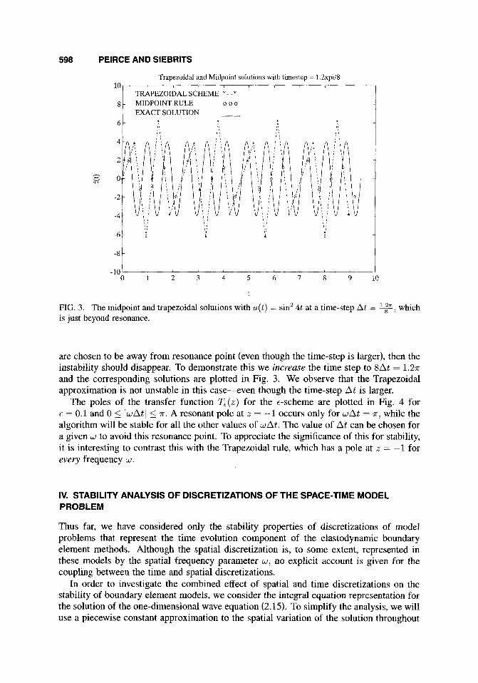
FIG. 3. The midpoint and trapezoidal solutions with u(t) = sin2 4t at a time-step At = 9, which is just beyond resonance.

are chosen to be away from resonance point (even though the time-step is larger), then the instability should disappear. To demonstrate this we increase the time step to 8At = 1 . 2 ~ and the corresponding solutions are plotted in Fig. 3. We observe that the Trapezoidal approximation is not unstable in this case-even though the time-step At is larger.

The poles of the transfer function T,(z) for the t-scheme are plotted in Fig. 4 for t = 0.1 and 0 5 IwAtl 5 IT. A resonant pole at z = -1 occurs only for wAt = T , while the algorithm will be stable for all the other values of wAt. The value of At can be chosen for a given w to avoid this resonance point. To appreciate the significance of this for stability, it is interesting to contrast this with the Trapezoidal rule, which has a pole at z = -1 for every frequency w.

IV. STABILITY ANALYSIS OF DISCRETIZATIONS OF THE SPACE-TIME MODEL PROBLEM

Thus far, we have considered only the stability properties of discretizations of model problems that represent the time evolution component of the elastodynamic boundary element methods. Although the spatial discretization is, to some extent, represented in these models by the spatial frequency parameter w, no explicit account is given for the coupling between the time and spatial discretizations.

In order to investigate the combined effect of spatial and time discretizations on the stability of boundary element models, we consider the integral equation representation for the solution of the one-dimensional wave equation (2.15). To simplify the analysis, we will use a piecewise constant approximation to the spatial variation of the solution throughout


Roots of the transfer function for the epsilon scheme

n LI \ / : : : : p i -1

-1 -0.5 0 0.5 1

FIG. 4. Poles of the transfer function for the t-scheme with 6 = 0.1

this section. The stability of various piecewise linear approximations to the time variation of the solution will be considered.

A. Spatial Semi-Discretization

We subdivide the spatial domain (-x, m) into elements each having a length Ax and assume that f ( < , 7) in (2.15) is constant over each subinterval. In this case, (2.15) reduces to

(4.1)

where


I t - r

X

FIG. 5. Light cone showing the elements and fractions of elements on which the point at the origin is dependent.

H is the Heaviside function, and T = % is the time period that it takes the wave to traverse one element. The function um(t) represents the influence at time t of the rnth element on the element that is centered at the origin. When the whole of the rnth element falls within the light cone centered at the origin then om = 1, whereas if only a portion of the element falls within the light cone, then om is the ratio of the part of the element in the light cone to Ax (see Fig. 5). This light cone information is all represented by means of the switches in the form of the Heaviside function in (4.2).

B. Fourier Transform of the Spatial Semi-Discretization

We notice that (4.1) involves a convolution sum over the spatial unknowns, which can be represented in the frequency domain as a multiplication of the Fourier transforms of u, and f m . This simplifies the stability analysis of the discrete algorithms substantially. To obtain this representation, we use the following pair of discrete Fourier transforms:

q w ) = F { U n }

= c e-iwxn U n n=-m

un = F-l{.iL(w)}

eZWxnti(w)dw, = "rAx ZIT - l r / A x

which we apply to (4.1) to obtain

(4.3)

(4.4)

At

2At

3At

4At

5At

6At

7At

8At

9At


N = O 1v=1 I v = 2 "3 - c

I T 12'1'

13T

1 4 7 '

FIG. 6. Light cone construction and values of N for the special case Q =

where t < l 7' - 2

where 0 = WAX, N ( t ) = [$ + i] - 1, and It] denote the function that evaluates the integer just less than t .

We note that the Volterra integral Eq. (4.4) is of a similar form to the modal model problem (2.1 I ) in which the kernel cosw(t - 7) has been replaced by the kernel &(w, t) defined in (4.5).

C. Fourier Transform of the Ramp Function

In this section we consider various piecewise linear approximations to (4.4). In Section IIIB we saw that the piecewise linear schemes can be conveniently constructed using the ramp function defined in (3.27). In a similar way, we use the following ramp integral as a basic building block for the analysis of piecewise linear time-stepping schemes:

h(t, At) = -&(w, t - T)&. I' i t After some manipulation, this integral can be reduced to the following form:

t 1 when - < -:

T - 2 t3

3AtT' R(t , At) = - t 1 when - > -: T 2

(4.6)


Spatial spectrum of 1D wave model: Q=1/2,1= 11 0.5

0.4

0.3

h

+4

4 0.2 v -

0.1

0

-0.1 0 0.1 0.2 0.3 0.4 0.5 0.6 0.7 0.8 0.9 1

t hct a/pi

FIG. 7. The analytic spatial spectrum Ji (0) of the constant-linear approximation (solid) compared with the spatial Discrete Fourier Transform of the constant-linear approximation (*).

T2 (2 - 3 cosec2g) + 6 [t - ( N + + ) I 2 s i n ( N + i ) o . + l2At sin 2

(4.7)

where 0 and N were defined below (4.5).

D. Stability of the Constant/Linear Scheme

The constant/linear scheme is obtained by applying the Trapezoidal rule to approximate the time integral in (4.1). In this case, the Fourier transform Eq. (4.4) assumes the form

(4.8)

where the kernel jl can be expressed as follows in terms of the ramp integral:

Sl(t9) = k(At( l + I), At) - 2k(AtZ, At) + k(At(Z - I), At). (4.9)

We observe that (4.8) involves a sum that is in the form of a z-transform convolution (see a-transform property 4 in Appendix A). Thus, by taking the z-transform of (4.8) we obtain the following simple algebraic equation representing the discretization of (2.15):

T 2 U ( z ) = - -J (z )F(z ) (4.10)


Zeros of J(z) for the Trapezoidal Scheme with Q=1/2

-4 -3 -2 -1 0 1 2 3 4

Re@)

FIG. 8. equation with Q = f .

Zeros of the transfer function J ( z ) for the constant-linear approximation of the wave

The stability of the discretization is determined by the poles of the transfer function A, or equivalently by the zeros of J ( z ) .

In order to obtain explicit expressions for J1 (O), it is necessary to make some specific assumptions about the relative magnitudes of the spatial meshing, the time meshing, and the wave velocity. The relationships among these three parameters can be determined by prescribing the value of the dimensionless mesh parameter Q = e. In the analysis presented in this work, we consider only two specific values Q = f and Q = 1. The first value, Q = f, represents the largest time-step for piecewise constant spatial elements for which the time-stepping can be performed explicitly, i.e., without inverting a matrix at each step. The second value, Q = 1, represents a time-step well into the implicit regime. An explicit scheme, Q = f , T = 2At: When determining an explicit expression for the function j l ( O ) , special care has to be taken to use the appropriate values of N in the formula (4.7). Figure 6 depicts the light cone for the case Q = f and the values of N as one moves away from an element on the wave front. In this case, & ( O ) can be expressed in the following form:

1 = 0

[sin (y) Bcot : + cos (9) 8 + cos (q) 01 , 1 odd . (4.11)

( Atsin (i) Ocot :, 1 even

In Fig. 7, we compare the function in (4.11) with the Discrete Fourier Transform of the actual constant/linear discretization of (2.15), whose discrete spectrum is denoted by asterisks.


Succesive trapezoidal solutions to 1 D wave equation 8 , I

Exact solution ---

Trapezoidal solution __ I

-1 -0.8 -0.6 -0.4 -0.2 0 0.2 0.4 0.6 0.8 I

X

FIG. 9. The constant-linear solution for the case Q = $.

In order to obtain the z-transform J ( z ) [see (4.10)J that applies in this case, we make use of (4.11) and the definition of the z-transform given in (A.1). After some simplification, we obtain

. (4.12) At[z4 + (5 + cos8)z3 + (6 + 4cos0)z2 + (5 + cos0)z + 11

6(z4 - 2 cos Oz2 + 1) J ( z ) =

As we described above, the stability of the constant/linear discretization of (2.15) in the case Q = is determined by the zeros of the function J ( z ) . In Fig. 8, the zeros of J ( z ) are plotted for the full range of values of 0: -7r 5 8 I n-. We note that, for each value of ~ , J ( z ) has one unstable root at z NN -3.732, one stable one at z NN 0.268, and a complex conjugate pair of roots are marginally stable so that the numerator of (4.12) factors as follows:

( z - eta(’))(z - e-ia(e))(z + 3.732)(z - 0.268).

In Fig. 9, the constant/linear numerical solution to (2.15) is compared to the analytic solution f(z, t) = sinvt sinzuz, which is the solution associated with the prescribed function

u(x,t) = . (4.13)

As predicted by the zeros of the above transfer function, we observe that the straight- forward constant/linear discretization of the one-dimensional wave equation leads to an unstable algorithm. In Fig. 10, the log of the amplitude of the numerical solution is also plotted for each time-step. The asymptotic gradient of this function is log(zll N” 1.32, which yields an estimate of the magnitude of the largest root z1 x -3.74. This agrees well with the value of the maximum root of the transfer function obtained from the stability

w[cosw(z - cc) - coszu(z + ct)] + cw[cos(vt + wz) - cos(vt - zuz)] 2CUI(V2 - c2w2)


Growth rate of the Trapezoidal instability

n

FIG. 10. The asymptotic growth rate of the constant-linear Q = $ solution.

analysis above. The question that remains unresolved is whether the scheme will become more stable when an implicit algorithm is used. To this end, we next consider an implicit scheme. An impkit scheme, Q = 1, T = At: Using a similar light cone diagram as that shown in Fig. 6 for the case Q = 1, j l ( 0 ) can be expressed in the form

$37 + 1 = Q

At (cot - q) sin10, ) I \ L 1 &(e) = (4.14)

Again, using the definition of the z-transform, we obtain

(4.15) At[(7+cos8)z2 + (22+10cos0)~+(7+cos8) ]

J ( z ) = 24( - 2 cos 82 + 1)

In Fig. 11, the zeros of J ( z ) are plotted for the full range of values of 0: -7r 5 0 5 7r.

As 0 varies from 7r to 0, the pole with the larger magnitude changes from being unstable at -3.8 to being stable at -0.2. Since there are unstable zeros for at least one of the possible values of the parameter 0 = wAz, the constant/linear discretization is unstable, in spite of the fact that the time-stepping scheme is implicit. The numerical solution in this case exhibits similar instabilities to that shown in Fig. 9.

E. Stability of the €-Scheme

Since both the explicit and implicit constandlinear schemes are unstable, we investigate the escheme to see if it yields improved stability characteristics as it did for the simpler model problems. We note that the t-scheme can be regarded as a perturbation to the


J @ , E ) = <

Zeros of J(z) for the Trapezoidal Scheme with Q=l

’ At( 1 + 3~ + 3e2 + c3 cos 0)/6, 1 = 0

at(5 + 3 ( ~ - E ~ ) + ((1 + E ) ~ - 2E3) cos8)/6, 111 = 1

At [sin (q) 0 (cot ; - sinO((1 + E ) ~ - 2 e 3 ) / 6 ) + ~ c o s ( ~ ) 8 ( 6 - ( l - ~ ) ~ + ( ( l + ~ ) ~ - 2 2 6 ~ ) ~ 0 ~ 8 ) ] , 111 > l o d d

1 at sin 0 cot; - $sine + [ ( 2 ) ( , 6 cos (i) 6)-4 + 6(1 + c ) ~ - 2(1 + E ) ~ + e3( l + C O S ~ ) ) ] , Ill 2 2 even.

-4 -3 -2 -1 0 1 2 3 4

W ) FIG. 11. equation with Q = 1.

Zeros of the transfer function J ( z ) for the constant-linear approximation of the wave


,-Q=1/2 and eps= 0 1 I

I I I

s , Q=1/2 and eps= 0.2

1

FIG. 12. Zeros of the transfer function J ( z , 6 ) for the c-scheme approximation of the wave equation with Q = f and 6 = 0 . 1 , ~ = 0 . 2 , ~ = 0.3, and t = 0.4.

Making use of the definition of the z-transform, we obtain the following expression for transfer function J ( z , E ) of the €-scheme:

z(z-l - 2 c o s e z 2 + 1) J ( z , 6 ) at

= (1 + 3c + 3E2 + 2 cose)25

+ [:, + (:OS e + 3( I + cos e)€ - 3 ( 1 - C O ~ e)f2 - 2 c o ~

+ [5 + - q i + cose)F - 3( i - cose)t2 + (1 + cose)E:3)z2

+ (1 - 3t + 3t2 + 2 ) z - 2. (4.18)

We note that the transfer function (4.18) for the t-scheme reduces to that of the Trapezoidal one (4.12) when E = 0. The zeros of the transfer function given in (4.18) are plotted in Fig. 12. We observe that the root structure in all these diagrams is similar to that given for the Trapezoidal constant/linear scheme in the case Q = $, which is plotted in Fig. 8. Increasing the parameter E brings the unstable zero closer to the unit disc until it finally falls within the unit disc for E 2 0.4. To demonstrate the validity of this analysis, in Fig. 13 we plot the 6-scheme solution for the cases E = 0.3, which is unstable, and the case E = 0.4, which is stable, as well as the exact solution.


Epsilon scheme approximates to exact solution f(x=-0.6,t)=sinvt.sin(-0.6~) for Q=In 8 -

-2 ‘ 0 0.1 0.2 0.3 0.4 0.5 0.6 0.7 0.8 0.9

t

FIG. 13. The exact solution and the Q = +€-scheme solutions with t = 0.3 and e = 0.4.

t-scheme Q = 1, T = Atl E 5 f : Making use of (4.16) and the appropriate light cone diagram for this case, the kernel j l ( 8 , t) can be expressed in the form

$ [4 + 6~ + 3(1 + 2 ~ ) ~ + (1 + 2 ~ ) ~ C O S ~ ] , 1 = 0

jl(8,t) = $ [ ( 2 3 + 6 t - 1 2 t 2 ) + 4 ( 6 + 9 t - 4 t 3 ) ~ ~ ~ 8 + ( 1 + 2 t ) 3 ~ ~ ~ 2 8 ] ( I 1 = 1

At [(cot C - sin8 (A + 2)) sinlo + E (2 - (1 + 26’) sin’ g ) c o ~ i e ) ] , 11) 2 2.

(4.19)

Making use of the definition of the z-transform, we obtain the following expression for transfer function J ( z , t) of the t-scheme:

i 24z(z2 - 2 cos 8z + 1) Jh €1 At

= [ (7 + cos 6 ) + 6( 3 + cos 6)t + 12( 1 + cos 6)t2 + 8 cos 8t3]z3 + [2(11+ 5c0s8) - 24(i + cos8)E2 - 8(i + 2cos8)t3]z2 + [ (7+c0s8) - 6 ( 3 + ~ 0 ~ 8 ) ~ + 1 2 ( 1 +cos8)t2 + 8 ( 2 + ~ ~ ~ 8 ) ~ ~ ] ~ - 8 ~ ~ . (4.20)

The transfer function (4.20) for the 6-scheme reduces to that of the Trapezoidal one (4.15) when E = 0. The zeros of the transfer function given in (4.15) have a similar structure to those in Fig. 11 and are plotted in Fig. 14. Once again, increasing the parameter E brings the unstable zeros closer to the unit disc until they finally fall within the unit disc for t > 0.366. In Fig. 15, we plot the exact solution and the escheme solution for the case E = 0.3, which is unstable, and the case E = 0.4, which is stable.


Q=l an*s 0 1 5 , Q=1 and7eps=0.2 I

I I

5 LA__. -5 0 5

5 ' , A 5 0 5

2 , Q=l and,eps= 0.3 , Q=1 and eps= 0.4 2 7 '

I

-21 --1- _ _ _ 2 0 2

2 I-_ I 2 0 2

FIG. 14. Zeros of the transfer funchon J ( z , c ) for the €-scheme approximation of the wave equation with Q = 1 and c = 0 .1 ,~ = 0 2 ,c = 0 3, and F = 0 4

V. CONCLUSIONS

Amid the growing evidence of numerical instabilities in boundary element elastodynamic models, there has hitherto been little theoretical investigation of the causes of these in-

Epsilon scheme approximates lo exact solution f(x=-0.6,t)=sinvt.sin(-0.6~) for Q=l 2.5

2

1.5

1

0.5 h a l o c

-0.5

- 1

-1.5

-2

1

FIG. 15. The exact solution and the Q = lc-scheme solutions with c = 0.3 and c = 0.4.

61 0 PEIRCE AND SlEBRlTS

stabilities and the possible strategies for remediation. Up till now, the user of a time domain BE algorithm had no way to guarantee a priori that a model with a given selection of meshing parameters would be stable. Indeed, there has been considerable frustration expressed in the literature [ I ] regarding the lack of predictability and alternative time- stepping procedures.

The objective of this article has been to address this lack of theory. Because of the complexity of the discretized boundary element equations, we have made use of a sequence of model problems in order to establish the appropriate tools to analyze the stability of existing time-stepping algorithms. The insight gained from these model problems has been useful in identifying the desirable properties that an improved time-stepping scheme should have. which has proved helpful in designing new time-stepping schemes with improved stability characteristics.

The basic device that we have used to perform the stability analysis is the z-transform. For the model problems considered, we were able to use the s-transform to reduce the time-convolution equations into a simple algebraic equation involving a transfer function that characterizes the stability properties of the algorithm in question.

In this article we have considered the stability properties of a variety of time-marching schemes when they are applied to three distinct model problems.

The simplest model problem is the one classically used by numerical analysts to investigate the stability properties of discrete approximations to Volterra integral equations (see for example [ 141). The stability analysis of boundary element type approximations applied to the classic model problem demonstrates quite clearly that the more stable schemes have larger or enhanced self effects-a property that is also important for more complicated boundary element models. However, the approximations to the model problem do not ex- hibit the type of exponential instability phenomena observed in actual boundary element models. This model problem was found to be inadequate as it does not give any account of the spatial discretization.

We then devised a new model problem that we referred to as the modal model problem. This model has Volterra-type time-stepping and attempts to represent the spatial discretization in terms of a single parameter w. Although this modal representation of the spatial information does not give any detailed account of the type of spatial approximation that is being used, the stability analysis does demonstrate additional possibilities for unstable behavior. The instabilities are in the form of resonances (giving polynomial growth with time) at certain spatial frequencies. However, this model does not manage to determine the source of the exponential instabilities observed in more general boundary element models.

We, therefore, considered a full space-time model problem based on the one-dimensional wave equation. A detailed stability analysis of the space-time discretizations of this model clearly demonstrated that exponential instabilities always occur for the Trapezoidal constant/linear discretization schemes. These results were verified numerically. The characteristic feature of this model problem, which is the source of the exponential instability, is that the Green’s function does not decay with space and time. Thus, close-coupling between neighboring and even remote elements leads to a situation in which the response of neighboring elements to a stimulus by a given element will involve more energy than the original signal. This positive feedback causes an exponential growth observed in all the numerical solutions. To remedy this situation, we devised a novel time-stepping scheme, named the c-scheme, which is a perturbation to the Trapezoidal constant/linear discretization. For this scheme, the self-effect of an element is enhanced while the other inter-

STABILITY ANALYSIS OF BE MODEL PROBLEMS 61 1

element influences remain largely unaltered. For a large enough choice of the parameter 6 , the constant/linear discretization becomes stable.

One key feature to emerge from the analysis of all these model problems was that the most stable schemes had self-effects that were larger than the other effects. The self-effect is the influence that an element or collocation point has on itself in the first time-step, whereas the influence an element has on itself at a later time, or the effects that an element has on one of its neighbors are referred to as "other effects," We exploited this insight to propose new time-stepping schemes with enhanced stability characteristics.

The tools and stability concepts developed in this article can be extended to enable them to be used for general boundary element models. As this article focuses on the analysis of model problems, this generalization will be treated in a future article.

APPENDIX A 2-TRANSFORM

Definition A.1. to be

The z-transform of a causal sequence { f k : f k = 0 if k < 0) is dejined

w

F ( z ) = z [ f k ] = f k z - ' , (A11

while the z-transform of a continuousfunction f ( t ) with the sampling period At is dejined to be

0

30

F ( z ) = Z [ f ( k A t ) ] = C f ( k A t ) z - ' . (A21 0

The z-transforms of some simple functions follow directly from the above definition.

Example 1. The z-transform of the Heaviside step function:

1 for t 2 0 0 for t < 0 H ( t ) =

is

Example 2. The z-transform of the exponential function:

Example 3. The z-transform of the siii function:

(A31

61 2 PEIRCE AND SlEBRlTS

Example 4. The a-transform of the cos function:

Although there are many more, we list only some of the important properties of the z-transform that we need in our stability analysis that follows. These properties can be derived from the definition of the z-transform.

Property 2. Backward shift:

Z [ f k ,,,I = z " Z [ f k ] .

Property 3. Forward shift:

Property 4. Convolution:

Lm -0 J

Property 5. Inversion integral: Let C be a closed contour enclosing all the poles of F ( z ) , (hen

The authors acknowledge the support of the Miningtek Laboratory of the Council for Scientific and Industrial Research of South Africa. The first author also acknowledges the support of the National Science and Engineering Research Council of Canada.

REFERENCES

1. D. J . Andrews, "Dynamic growth of mixed-mode shear cracks," Buff. Seism. SOC. Am. M, I184 ( I 994).


2.

3.

4.

8.

9.

10.

11

12.

13.

14.

15.

16.

17.

18.

19.

M. G. Mack, “A three-dimensional boundary element method for elastodynamics,” Ph. D. Thesis, University of Minnesota, 1991.

E. Siebrits, “Two-dimensional time domain elastodynamic displacement discontinuity method with mining applications,” Ph. D. Thesis, University of Minnesota, 1992.

Y. Tian, “Boundary element method in elastodynamics,” Ph. D. Thesis, University of Minnesota, 1990.

M. C. Loken, “A three-dmensional boundary element method for linear elastodynamics,” Ph. D. Thesis, University of Minnesota, 1992.

J. Dominguez, Boundary elements in dynamics, Computational Mechanics Publications, Southampton, ( 1 993).

H. L. Selberg, “Transient compression waves from spherical and cylindrical cavities,” Arkiv for Fysik 5, 97 (1951).

M. G. Koller, M. Bonnet, and R. Madariaga, “Modelling of dynamical crack propagation using time-domain boundary integrals,” Wave Motion 16, 339 (1992).

A. P. Peirce and E. Siebrits, “Stability analysis and design of time-stepping schemes for general elastodynamic boundary element models,” Int. J. Num. Meth. Eng., to appear.

S. Kobayashi, “Fundamentals of boundary integral equation methods in elastodynamics,” in Topics in boundary element research, 1101. 2: Time-dependent and vibration problems, Brebbia, Ed., Springer-Verlag, New York, p. 1, 1985. P. K. Banerjee, S. Ahmad, and G. D. Manolis, “Advanced elastodynamic analysis,” in Boundary Element Methods in Mechanics, Beskos, Ed., Elsevier Science Publishers B.V., Amsterdam, p. 258, 1987.

A. C. Eringen and E. S. Suhubi, Elastodynamics: Volume I1 Linear Theory, Academic Press, New York, 1975.

C. T. H. Baker, Numerical Treatment of Integral Equations, Oxford University Press, Oxford (1977).

C. T. H. Baker and N. J. Ford, “Some applications of the boundary-locus method and the method of D-partitions,” IMA J. Num. Anal. 11, 143 (1991).

E. I. Jury, Theory and Application of the z-Transfonn Method, Krieger, Florida, 1986.

K. Ogata, Discrete-7ime Control Systems, Prentice-Hall, New Jersey, 1987.

L. Sirovich, Introduction to Applied Mathematics, Springer-Verlag, New York, 1988.

W. H. Press, S. A. Teukolsky, W. T. Vetterling, and B. P. Flannery, Numerical Recipes, 2nd Ed, Cambridge University Press, New York, 1992.

A. P. Peirce, S. Spottiswoode, and J. A. L. Napier, “The spectral boundary element method: a new window on boundary elements in rock mechanics,” Int. J. Rock Mech. Min. Sci. & Geomech. A b s ~ , 29, 379 (1992).

Stability analysis of model problems for elastodynamic...

Documents

Transcript of Stability analysis of model problems for elastodynamic...