Stability Analysis and Design of Nonlinear Sampled-Data ...

INTERNATIONAL JOURNAL OF ROBUST AND NONLINEAR CONTROLInt. J. Robust. Nonlinear Control 2010; 00:1–23Published online in Wiley InterScience (www.interscience.wiley.com). DOI: 10.1002/rnc

Stability Analysis and Design of Nonlinear Sampled-DataSystems Under Aperiodic Samplings

K.Hooshmandi1, F. Bayat2∗†, M. R. Jahed-Motlagh1, A. A. Jalali1

1Department of Electrical Engineering, Iran University of Science and Technology, Tehran, Iran.

2Department of Engineering, University of Zanjan, Zanjan, Iran.

SUMMARY

In this paper, the problem of exponential stability analysis and design of sampled-data nonlinear systemshave been studied using a polytopic LPV approach. By means of modeling a new double-layer polytopicformulation for nonlinear sampled-data systems, a modified form of piecewise continuous Lyapunov-Krasovskii functional is proposed. This approach provides less conservative robust exponential stabilityconditions by using Wirtingers inequality in terms of linear matrix inequalities. The distances betweenthe real continuous parameters of the plant and the measured parameters of the controller are modeledby convex sets, and the analysis/design conditions are given at the vertices of some hyper-rectangles. Inorder to get tractable LMI conditions for the stabilization problem, we performed relaxation by introducinga slack variable matrix. Under the new stability criteria, an approach is introduced to synthesize a sampled-data polytopic LPV controller considering some constraints on the location of the closed-loop poles in thepresence of uncertainties on the varying parameters. It is shown that the proposed controller guaranteesthe exponential stability of the closed-loop system for aperiodic sampling periods smaller than a knownvalue, i.e. maximum allowable sampling period (MASP). Finally, the effectiveness of the proposed approachis verified and compared with some state-of-the-art existing approaches through numerical simulations.Copyright c© 2010 John Wiley & Sons, Ltd.

KEY WORDS: Nonlinear sampled-data systems; LPV systems; Lyapunov-Krasovskii functional;Wirtingers inequalities; LMI method.

1. INTRODUCTION

In many practical applications, the use of communication channels to implement control algorithmshas considerably increased. In such applications, a heavy temporary load of computation in aprocessor and communication constraints can corrupt the sampling period of a given controller.Therefore, the variation of the sampling period will affect the stability and the performance of theclosed loop system. So, it is quite important to determine a maximum allowable delay that the closedloop system remains stable for a given controller [1, 2, 3, 4]. The sampled-data control systemsare prevalent approaches for stability analysis and controller design for systems under aperiodicsampling. Different techniques, including lifting approach [5], robust approach [6], impulsive modelapproach [7, 8], looped-functional approach [9, 10] and the input delay approach [11, 12], have beenused to address the linear sampled-data systems and focused on only aperiodic sampling aspectwhich suitable for networked control systems.

∗Correspondence to: Farhad Bayat, Associate professor, University of Zanjan.†E-mail: [email protected]

Copyright c© 2010 John Wiley & Sons, Ltd.Prepared using rncauth.cls [Version: 2010/03/27 v2.00]

This article is protected by copyright. All rights reserved.

This is the author manuscript accepted for publication and has undergone full peer review buthas not been through the copyediting, typesetting, pagination and proofreading process, whichmay lead to differences between this version and the Version of Record. Please cite this articleas doi: 10.1002/rnc.4043

http://dx.doi.org/10.1002/rnc.4043

http://dx.doi.org/10.1002/rnc.4043

2

Nonlinear sampled-data systems arise when either the plant model or the controller is nonlinear.While their linear counterpart is now a mature area, nonlinear sampled-data systems are muchharder to deal with and, hence, much less studied. Therefore, there are a few references in theliterature of nonlinear sampled-data systems where the input delay model [13, 14] or hybrid model[15] of the system is studied. Their inherent complexity leads to a closed-loop system which ismathematically involved [13, 14, 15] and thus, can not be directly used to design a controller thatprovides a desired maximum allowable sampling periods (MASP). They only developed Lyapunov-like sufficient conditions for robust global asymptotic stability or input-to-output stability of agenerally nonlinear sampled-data system. In contrast, [16, 17] provide linear state feedback sampleddata controller design condition for nonlinear system with sector-bounded nonlinearity based on theinput delay approach and using a different LKF. The polytopic LPV (PLPV) systems are suitablefor the sampled-data control of nonlinear systems since many nonlinear systems can be modeledby a linear system with some time varying parameters [18, 19]. As a consequence, some powerfuldesign methods in the linear systems can be effectively extended to the PLPV systems, so thatstability analysis and design condition with sampled-data PLPV state feedback controller lead toconvex optimization problem in the framework of LMIs. Using PLPV model for stability analysisand design of nonlinear sampled-data systems faces the challenge of non-compliance between theactual and the measured parameters. This issue is addressed in this paper by analyzing the impactof the sampling interval and the rate of parameters variations on the stability and stabilization of theclosed-loop sampled-data system where the system is described by a double-layer polytopic model.

In the context of LPV systems, there are few research papers formally addressing the analysisof the sampled-data problem. In [20, 21], assuming that the parameters do not vary in the intervalbetween consecutive sampling, a lifting technique is applied to derive stability conditions. A time-delay approach is utilised by [22, 23, 24] for sampled-data controller design of continuous time LPVsystems through mapping the hybrid closed-loop system to a continuous-time state-delayed LPVsystem. Stability conditions are derived using a smooth LKF which utilised in stability analysis ofsystems with fast varying input delays. Reference [22] considered the sampled parameter vector as anew parameter which make the optimization problem corresponding to the sampled-data controllerdesign so conservative while in [23, 24] it is assumed that the time-varying parameters are constantbetween two consecutive samples which is restricted to slowly parameter varying systems. [25]and [26] addressed the problem of sampled-data MPC for PLPV system in the form of impulsivemodel. The sampled parameter vector is considered as a new parameter which is the price to pay forimperfect knowledge of the sampled parameter. Also, heavy online computation is required in theproposed methods because a set of LMIs must be solved at each sampling instant to determine thecontrol law. Contrary to the previous approaches, [27] utilized the sampling effect of the schedulingparameter for affine LPV systems where the input matrix does not depend on the parameters.Therefore, this approach cannot be utilized for all class of the PLPV systems. Also, the idea ofdefining of the system dynamics during the sampling interval inspired in the field of linear impulsivesystems [9]. However, applying this approach requires that the parameters vector to be constantduring the sampling intervals which is clearly in contradiction with the goal of analyzing the impactof parameters sampling on the stability of the closed-loop system.

Most of the previous studies in the field of sampled-data LPV systems assumed that the parametervector is constant in between two consecutive samples whereas this assumption is only valid forsystems with slowly varying parameters and small sampling periods. Therefore, it can not coverapplications such as network control systems with aperiodic sampling. For convenience of study,in some attempts in the literature of sampled-data LPV control systems the sampled parameter isconsidered as a new parameter which is quite conservative and is a major limitation for improvingperformance. In addition, the effects of the scheduling parameters sampling on the performanceand transient behaviors of the closed loop system is another important subject that needs to becarefully considered. To fill these gaps, in this paper the uncertainty of the measured parameters inthe controller are transferred to that of the plant parameters and the closed-loop sampled-data PLPVsystem is represented by a double-layer polytopic uncertain model. This technique can be applied to

Copyright c© 2010 John Wiley & Sons, Ltd. Int. J. Robust. Nonlinear Control (2010)Prepared using rncauth.cls DOI: 10.1002/rnc


3

a large class of multi model systems like Takagi-sugeno(T-S) model [28] which gives an effectiveway to represent complex nonlinear systems by some simple local linear dynamic systems.

The main contribution of this paper is to present exponential stability analysis and designcriteria for nonlinear sampled-data systems under aperiodic samplings based on the PLPV modelingapproach. By introducing a new double-layer polytopic formulation for nonlinear sampled-data sys-tems, a candidate discrete Lyapunov-Krasovskii functional is proposed which, by using Wirtingersinequality, provides less conservative robust stability conditions than the existing approaches. Underthe new stability criteria, an approach is introduced to synthesize a sampled-data PLPV controllerconsidering some constraints on the location of the closed-loop poles in the presence of uncertaintieson the varying parameters.

The paper is organized as follows. Section 2 presents the problem formulation and someassumptions used in this paper. Section 3 presents the derivation of exponential stability conditionfor sampled-data PLPV systems. In section 4 the problem of pole placement for sampled-data PLPVcontroller with aperiodic sampling time is stated. Numerical examples and conclusion are given insections 5 and 6, respectively.

Notation. Throughout the paper, sets of real numbers, nonnegative real numbers, real vectors ofdimension n, matrices of dimension n×m, symmetric and symmetric positive definite matrices ofdimension n are denoted byR,R+,Rn,Rn×m, Sn and Sn+ respectively. ‖.‖ stands for the Euclideannorm of a vector. For any square matrix A ∈ Rn×n, we define He(A) = A+AT . The notationP > 0, for P ∈ Rn×n, means that P is symmetric and positive definite. For symmetric matrices Xand Y ,X < Y means thatX − Y is negative definite. The notation I and 0 stand for the identity andzero matrices of appropriate dimensions. The symmetric elements of any symmetric matrix denotedby ∗. For a given positive number T , let W : [−T, 0]→ Rn be the space of absolutely continuousfunctions, with square integrable first order derivatives mapping the interval [−T, 0] toRn. Considerfunction xt ∈W defined as xt(θ) = x(t+ θ), θ ∈ [−T , 0] . Similar to [11], we denote the norm ofxt by

‖xt‖W = maxθ∈[−T,0]

‖xt(θ)‖+

0∫−T

‖xt(q)‖2dq

0.5

. (1)

2. PROBLEM FORMULATION

Linear parameter varying systems are a class of systems whose state space matrices depend on atime-varying parameter vector η : R+ → Rnη . It is assumed that, the parameter vector η(t) variescontinuously and its derivative is bounded. Define

Φ :=η : R+ → Rnη |η(t) ∈ ∆η, η(t) ∈ ∆v

(2)

where ∆η and ∆v are respectively the set of admissible parameter and its derivative. We also assumethat the sets ∆η and ∆v are compact and convex polyhedrons and bounded as follows:

∆η =η : R+ → Rnη |mi ≤ ηi(t) ≤ mi, i = 1, ..., nη

∆v =

η : R+ → Rnη |vi ≤ ηi(t) ≤ vi, i = 1, ..., nη

(3)

The state space model of LPV systems, defined as:

x(t) = A(η(t))x(t) +B(η(t))u(t) (4)

where x(t) ∈ Rnx is the state vector and u(t) ∈ Rnu is the control input vector.In the polytopic representation, the system state-space matrices take values inside a polytope

which is the convex hull of the parameters of a set of models, called vertex models. The system



4

matrices are given by

A(η(t)) =

N∑i=1

αi(t)Ai B(η(t)) =

N∑i=1

αi(t)Bi. (5)

where the time-varying parameters are given by η(t) =∑N

i=1 αi(t)Λi where Λi (vertices of thepolytope) are the extremal values of η(t) and αi(t) are the time-varying polytopic coordinatesevolving over the unit simplex Σ which is defined as

Σ =

α(t) = col (αi(t)) :

N∑i=1

αi(t) = 1, αi(t) ∈ [0, 1] , N = 2nη

. (6)

Any LPV system can be represented, up to a certain degree of accuracy, by a PLPV system.Whenever the matrices of the LPV system are affinely depend on η(t), there exists a linearrelationship between η(t) and α(t) that can be easily determined from the physical model.

As shown in Fig. 1 the controller output at each sampling instant is updated based on the value ofthe state vector and the corresponding LPV parameter vector, so the control signal will be piecewiseconstant. We consider the following polytopic state feedback controller:

u(t) = u(tn) =

N∑i=1

αi(tn)Kix(tn) t ∈ [tn, tn+1) , n ∈ N (7)

where, Ki denotes the i-th controller gain at the i-th vertex of the polytope that need to bedetermined. Then the closed-loop interconnection of Eq.(4) and Eq.(7) is

x(t) =

N∑i=1

αi(t)Aix(t) +

N∑i=1

αi(t)Bi

N∑i=1

αi(tn)Kix(tn). (8)

In networked setting, the effect of the network and aperiodic sampling period are integrated in asingle input-delay value τ(t). We model the sampled-data structure as a time-varying delay in theinput. The delay induced by the sampler is defined by:

τ(t) = t− tn for t ∈ [tn, tn+1) , n ∈ N, (9)

Sampling

Continuous

LPV Plant

Sampled-Data

LPV Controller

Sampling

ZOH

( )t

( )x t( )u t

Continuous LPV Controller

( )nx t( )nu t

( )nt

Figure 1. Closed-loop LPV sampled-data system.



5

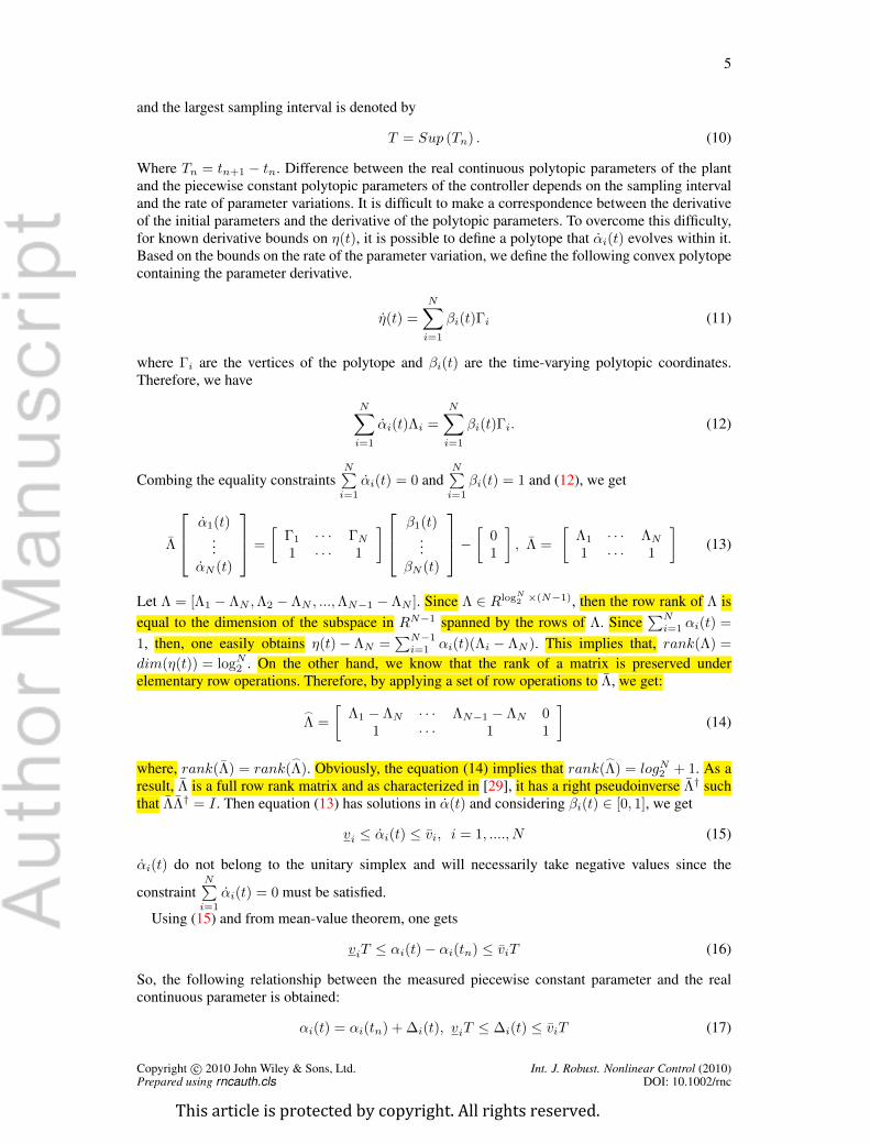
and the largest sampling interval is denoted by

T = Sup (Tn) . (10)

Where Tn = tn+1 − tn. Difference between the real continuous polytopic parameters of the plantand the piecewise constant polytopic parameters of the controller depends on the sampling intervaland the rate of parameter variations. It is difficult to make a correspondence between the derivativeof the initial parameters and the derivative of the polytopic parameters. To overcome this difficulty,for known derivative bounds on η(t), it is possible to define a polytope that αi(t) evolves within it.Based on the bounds on the rate of the parameter variation, we define the following convex polytopecontaining the parameter derivative.

η(t) =

N∑i=1

βi(t)Γi (11)

where Γi are the vertices of the polytope and βi(t) are the time-varying polytopic coordinates.Therefore, we have

N∑i=1

αi(t)Λi =

N∑i=1

βi(t)Γi. (12)

Combing the equality constraintsN∑i=1

αi(t) = 0 andN∑i=1

βi(t) = 1 and (12), we get

Λ

α1(t)...

αN (t)

=

[Γ1 · · · ΓN1 · · · 1

] β1(t)...

βN (t)

− [ 01

], Λ =

[Λ1 · · · ΛN1 · · · 1

](13)

Let Λ = [Λ1 − ΛN ,Λ2 − ΛN , ...,ΛN−1 − ΛN ]. Since Λ ∈ RlogN2 ×(N−1), then the row rank of Λ isequal to the dimension of the subspace in RN−1 spanned by the rows of Λ. Since

∑Ni=1 αi(t) =

1, then, one easily obtains η(t)− ΛN =∑N−1

i=1 αi(t)(Λi − ΛN ). This implies that, rank(Λ) =

dim(η(t)) = logN2 . On the other hand, we know that the rank of a matrix is preserved underelementary row operations. Therefore, by applying a set of row operations to Λ, we get:

_

Λ =

[Λ1 − ΛN · · · ΛN−1 − ΛN 0

1 · · · 1 1

](14)

where, rank(Λ) = rank(_

Λ). Obviously, the equation (14) implies that rank(_

Λ) = logN2 + 1. As aresult, Λ is a full row rank matrix and as characterized in [29], it has a right pseudoinverse Λ† suchthat ΛΛ† = I . Then equation (13) has solutions in α(t) and considering βi(t) ∈ [0, 1], we get

vi ≤ αi(t) ≤ vi, i = 1, ...., N (15)

αi(t) do not belong to the unitary simplex and will necessarily take negative values since the

constraintN∑i=1

αi(t) = 0 must be satisfied.

Using (15) and from mean-value theorem, one gets

viT ≤ αi(t)− αi(tn) ≤ viT (16)

So, the following relationship between the measured piecewise constant parameter and the realcontinuous parameter is obtained:

αi(t) = αi(tn) + ∆i(t), viT ≤ ∆i(t) ≤ viT (17)



6

Since,N∑i=1

αi(t) = 1 andN∑i=1

αi(tn) = 1 therefore we getN∑i=1

∆i(t) = 0. Then,by replacing Eq.(17)

in Eq.(8) we get

x(t) =

N∑i=1

λi(t) (Ai + ∆A(t))x(t) +

N∑i=1

λi(t) (Bi + ∆B(t))

N∑i=1

λi(t)Kix(t− τ(t)) (18)

Where

∆A(t) =

N−1∑j=1

∆j(t) (Aj −AN ),∆B(t) =

N−1∑j=1

∆j(t) (Bj −BN )

λi(t) = αi(tn) = αi(t− τ(t)) (19)

In this way, the uncertainty on the measured parameters of the controller is turned into theparameters of the plant and the closed-loop sampled-data LPV system represented by a double-layerpolytopic description model as illustrated in Fig. 2. The first polytope represents a LPV system ineach vertex where the LPV controller is designed for sampled-data of varying parameters shown asnominal vertex A1, A2, A3, A4. The second polytop is constructed at each vertex of the system inorder to model uncertainty of the varying parameters proportional to sampling period and the rate ofparameter variations as shown by A1,1, A1,2A1,3 around the first nominal vertex A1. It is obviousthat the systems(8) and (18) are equivalent. Thus, the stability analysis and design problems of (8)can be transformed to the same problem of (18), that can be easily verified using convex optimizationtechniques at the vertices of the model. To the best of the authors knowledge, this formulation forsampled-data LPV systems has not already been addressed in the literatures.

1( )

kt

2(

)kt

3 ()k

t

4 ()k

t

A

1,1A

1,2A

1,3A

4,1A

4,2A4,3A

3,3A

3,2A

3,1A

2,1A

2,2A

2,3A

3A1A

4A

2A

Figure 2. Double-layer polytopic description of PLPV sampled-data system.

3. EXPONENTIAL STABILITY CRITERIA

In this section, the problem of exponential stability analysis for system in Eq.(18) is addressed.It is assumed that the feedback gain matrices Kj have been well designed. In the following thesufficient conditions are formulated in terms of LMIs to find the MASP that preserves the closed-loop system’s exponential stability provided that the controller is implemented in a sample-and-hold



7

fashion. In the following we decoupled LKF matrix functions and system matrices which allows usto achieve robust exponential stability results. Before starting exponential stability analysis, thefollowing lemmas which will be used in the proofs of our results are presented.

Lemma 1 ([11])Let there exist positive numbers β, δ and functional V : R×W × L2 [−T, 0]→ R such that

β‖xt(0)‖2 ≤ V (t, xt, xt) ≤ δ ‖xt‖2W . (20)

Let the function V (t) = V (t, xt, xt) is continuous from the right for xt satisfying Eq.(18), absolutelycontinuous for t 6= tn and satisfies limt→t−n V (t) ≥ V (tn). If along Eq.(18)

˙V (t) ≤ −σ V (t) (21)

then system in Eq.(18) is exponentially stable with the decay rate σ/2 and µ =√δ/β.

Lemma 2 ([30])For matrices M , N and R > 0 with appropriate dimensions, the following inequality holds.

MN +NTMT ≤MRMT +NTR−1N. (22)

Lemma 3 ([31])(Wirtinger inequality) For a given matrixR ∈ Sn+, the following inequality holds for all continuouslydifferentiable function x ∈ [a, b]→ Rn:∫ b

a

xT (t)Rx(t)dt ≥ 1

b− a(x(b)− x(a))

TR(x(b)− x(a)) +

3

b− aΩTRΩ (23)

Where Ω = x(b) + x(a)− 2b−a

∫ bax(t)dt.

The next theorem provides conditions for exponential stability of the PLPV system in the Eq.(18).In some cases, for the sake of simplicity, explicit dependence on t omitted to shorten the notation.

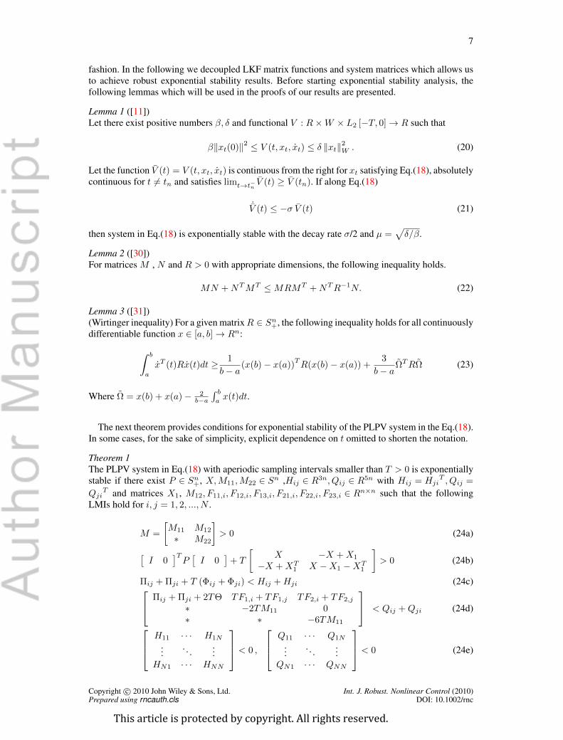
Theorem 1The PLPV system in Eq.(18) with aperiodic sampling intervals smaller than T > 0 is exponentiallystable if there exist P ∈ Sn+, X,M11,M22 ∈ Sn ,Hij ∈ R3n, Qij ∈ R5n with Hij = Hji

T , Qij =

QjiT and matrices X1, M12, F11,i, F12,i, F13,i, F21,i, F22,i, F23,i ∈ Rn×n such that the following

LMIs hold for i, j = 1, 2, ..., N .

M =

[M11 M12

∗ M22

]> 0 (24a)

[I 0

]TP[I 0

]+ T

[X −X +X1

−X +XT1 X −X1 −XT

1

]> 0 (24b)

Πij + Πji + T (Φij + Φji) < Hij +Hji (24c) Πij + Πji + 2TΘ TF1,i + TF1,j TF2,i + TF2,j

∗ −2TM11 0∗ ∗ −6TM11

< Qij +Qji (24d)

H11 · · · H1N

.... . .

...HN1 · · · HNN

< 0 ,

Q11 · · · Q1N

.... . .

...QN1 · · · QNN

< 0 (24e)



8

Where

Πij(1, 1) = He (P (Ai + ∆A(t))− F11,i − 3F21,i)−XΠij(1, 2) = P (Bi + ∆B(t))Kj −X1 +X + F11,i − FT12,i − 3F21,i − 3FT22,i −M12

Πij(1, 3) = −FT13,i + 6F21,i − 3FT23,iΠij(2, 2) = −X +He

(X1 + F12,i − 3FT22,i +M12

)Πij(2, 3) = FT13,i + 6F22,i − 3FT23,i, Πij(3, 3) = 6F23,i + 6FT23,iΘ = −

[0 I 0

]TM22

[0 I 0

]Φij(1, 1) = He (X (Ai + ∆A(t))) +

(ATi + ∆T

A(t))M11 (Ai + ∆A(t))

Φij(1, 2) =(ATi + ∆T

A(t))

(X1 −X +M12 +M12(Bi + ∆B(t))Kj) +X(Bi + ∆B(t))Kj

Φij(2, 2) = He((XT

1 −X +MT12

)(Bi + ∆B(t))Kj

)+

M22 +KTj (BTi + ∆T

B(t))M11(Bi + ∆B(t))Kj

Φij(1, 3) = Φij(2, 3) = Φij(3, 3) = 0

ProofAt the first step, we consider the following LKF for exponential stability analysis:

V (t) = V1(t) + V2(t, xt, xt) + V3(t, xt) t ∈ [tn, tn+1) (25)

V1(t) = xT (t)Px(t)

V2(t) = (tn+1 − t)∫ t

tn

[x(q)x(tn)

]TM

[x(q)x(tn)

]dq

V3(t) = (tn+1 − t)ξT (t)

[X −X +X1


1

]ξ(t)

Where ξT (t) =[xT (t), xT (tn)

].

We utilized, a piecewise smooth LKF which decreases the conservatism of the stability conditionswhen compared with a smooth LKF used for input delay approaches in [24, 32]. Performance ofLKF is intuitive, therefore we will show that the proposed structure lead to less conservative stabilityconditions. Based on Lemma 1, the candidate LKF must be right continuous. In the followinglemma, right continuity property of the LKF in Eq.(25) is presented.

Lemma 4The KFL defined in Eq.(25) is a right continuous and non increasing function of time at samplinginstant tn.

ProofWe assume that decision matrix P , M , X , X1 are chosen in such a way that condition in Eq.(20)satisfied. Obviously, the Lyapunov function V1 has quadratic form and thus is continuous. V2 iscontinuous between two sampling instants, so they are non-negative at t−n . At instant tn, the lowerand upper bounds of the integral become equal, thus V2 get zero. Also,V3 is continuous between twosampling instants and is non-negative at t−n . At the instants tn, because of x(t) = x(tn), V3 get zero.Therefore, the condition

limt→t−n V (t) ≥ V (tn) (26)

holds.After sampling, since lim

t→tn+τ(t) = τ(tn) = 0 then t = tn, and we have

limt→tn+

V2(t) + V3(t) = 0. (27)

Thus V (t) is right continuous in time since limt→tn+

V (t) = V (tn).



9

In the following, we compute lower and upper bounds of candidate LKF to ensure that inequalityin Eq.(20) satisfied. Constraint (24a) is sufficient conditions for positiveness of integral terms. Bycombination non-integral terms, we get

V1 + V3 = ξT (t)Ψξ(t), t ∈ [tn, tn+1)

Ψ =[I 0

]TP[I 0

]+ (tn+1 − t)

[X −X +X1


1

](28)

Since P > 0 and Eq.(24b) are sufficient condition for existence small β such that

β‖x(t)‖2 = β‖xt(0)‖2 ≤ V (t). (29)

Using the inequalities ‖x(t)‖ ≤ ‖xt‖W and ‖ξ(t)‖ ≤√

2 ‖x(t)‖ in Eq.(28), one gets

V1(t) + V3(t) ≤ 2λmax (Ψ) ‖xt‖2W . (30)

Also for V2(t), we have

V2 ≤ Tλmax (M)

(∫ t

tn

‖x(q)‖2dq +

∫ t

tn

‖x(tn)‖2dq)

(31)

Considering∫ 0

−T ‖xt(q)‖2dq ≤ ‖xt‖2W from Eq.(1) we can write

V2 ≤ Tλmax (M) (1 + T ) ‖xt‖2W(32)

Adding inequalities in Eq.(30) and Eq.(32) the upper bound on V (t) is obtained as

V (t) ≤2λmax (Ψ) + T (λmax (M))(1 + T )‖xt‖2W . (33)

Consequently, inequalities in Eqs.(29) and (33) guarantee the condition in Eq.(20).The exponential stability and stabilization conditions are derived from the time derivative of LKF.

Therefore candidate LKF must satisfy inequalities in Eq.(21). The derivative of Lyapunov functionV1(t) along the system trajectory is given by

V1 = xT(N∑i=1

λiHe (P (Ai + ∆A(t)))

)x+ xT (tn)

(N∑

i,j=1

λiλjP (Bi + ∆B(t))Kj

)x

+xT

(N∑

i,j=1

λiλjKTj (Bi + ∆B(t))

TP

)x(tn)

(34)

Also the derivative of Lyapunov function V3(t, xt) along the system trajectory is given by

V3 = ξT[X −X +X1

∗ X −X1 −XT1

]ξ+

(tn+1 − t)ξT(N∑i=1

λi

[He (X (Ai + ∆A(t))) (Ai + ∆A(t))

T(−X +X1)

∗ 0

])ξ+

(tn+1 − t)ξT(

N∑i,j=1

λiλj

[0 X (Bi + ∆B(t))Kj

∗ He ((−X +X1) (Bi + ∆B(t))Kj)

])ξ

(35)

Differentiating V2(t, xt, xt) along the system trajectory, we get

V2 = (tn+1 − t)xT (t)M11x(t) + xT

(N∑i=1

λi2(Ai + ∆A(t))TM12

)x(tn)

+(tn+1 − t)

xT (tn)

N∑i,j=1

λiλj2((Bi + ∆B(t))Kj)TM12x(tn) + xT (tn)M22x(tn)

−∫ ttnxT (q)M11x(q)dq − 2 (x(t)− x(tn))M12x(tn)− τxT (tn)M22x(tn)

(36)



10

Since M11 is positive definite, it can be rewritten as M11 = M0.511 M

0.511 . Using Eq.(18), we get

xTM11x = 0.5N∑

i,j,n,l=1

λiλjλnλl

(ξT[

ATi + ∆TA

KTj

(BTi + ∆T

B

) ]M0.511 M

0.511 [Al + ∆A (Bl + ∆B)Kn] ξ

)+0.5

N∑i,j,n,l=1

λiλjλnλl

(ξT[

ATl + ∆TA

KTn

(BTl + ∆T

B

) ]M0.511 M

0.511

[Ai + ∆A (Bi + ∆B)Kj

]ξ

)(37)

Applying Lemma 2 on (37), with considering

N = M0.511 [Al + ∆A (Bl + ∆B)Kn]

MT = M0.511

[Ai + ∆A (Bi + ∆B)Kj

], R = I (38)

the following inequality obtained.

xTM11x <

N∑i,j=1

λiλjξT

[ (ATi + ∆T

A

)M11 (Ai + ∆A)

(ATi + ∆T

A

)M11 (Bi + ∆B)Kj

∗(KTj

(BTi + ∆T

B

))M11 (Bi + ∆B)Kj

]ξ

(39)

By defining vector ζ(t) as

ζ(t) =[x(t) x(tn)

∫ ttnx(q)dq

τ(t)

](40)

and using Lemma (3), we have

−∫ ttnxT (q)M11x(q)dq ≤ − 2

τ(t)ζT(W1M11W

T1 + 3W2M11W

T2

)ζ

WT1 =

[I −I 0

], WT

2 =[I I −2I

] (41)

By using Lemma. (2), the following inequalities replaced in Eq(41)

F1 (λ)WT1 +W1F

T1 (λ) ≤ 2

τ(t)W1M11WT1 + τ(t)

2 F1 (λ)M−111 FT1 (λ)

F2 (λ)WT2 +W2F

T2 (λ) ≤ 2

τ(t)W2M11WT2 + τ(t)

2 F2 (λ)M−111 FT2 (λ)

FT1 (λ) =N∑i=1

λi[FT11,i FT12,i FT13,i

], F2 (λ) =

N∑i=1

λi[FT21,i FT22,i FT23,i

] (42)

Therefore ˙V (t) yields

˙V (t) = V1(t) + V2(t) + V3(t) ≤N∑

i,j=1

λiλjζT (Πij + (T − τ) Φij + τΘ)ζ+

τζT(F1M

−111 F

T1 + 3F2M

−122 F

T2

)ζ

(43)

For τ = 0, Eq.(24c) and Eq.(24e) implies

˙V (t) ≤ ζT (N∑i=1

λi2 (Πii + TΦii) +

N∑i=1

N∑i<j

λiλj (Πij + Πji + T (Φij + Φji)))ζ < λ1ζ...

λNζ

T H11 · · · H1N

.... . .

...HN1 · · · HNN

λ1ζ

...λNζ

< −α1

N∑i=1

λi2ζT ζ < −α1ζ

T ζ

(44)



11

Also for τ = T , by applying Schur complement to Eq.(43) thus Eq.(24d) and Eq.(24e) implies

˙V (t) ≤ ζT N∑i=1

λ2i

Πii + TΘ TF1,i TF2,i

∗ −TM11 0∗ ∗ −3TM11

+

N∑i=1

N∑i<j

λiλj

Πij + Πji + 2TΘ TF1,i + TF1,j TF2,i + TF2,j

∗ −2TM11 0∗ ∗ −6TM11

ζ < λ1ζ...

λN ζ

T Q11 · · · Q1N

.... . .

...QN1 · · · QNN

λ1ζ

...λN ζ

< −α2

N∑i=1

λ2i ζT ζ < −α2ζ

T ζ

ζT =[ζT ζT ζT

]

(45)

Where α1 > 0, α2 > 0. Since Eq.(43) is affine in τ , then there exists a small scalar c > 0 such that˙V (t) < −c ‖xt‖2W to hold for any instants t ∈ [tn, tn+1). ˙V (t) < −c ‖xt‖2W using Eq.(20) implied˙V (t) < −cδ V (t). Then system in Eq.(18) is exponentially stable with the decay rate c/2δ. With

this completes the proof.

Remark 1Here we could extend the stability conditions of LIT sampled-data systems given in [11] and [33]to the PLPV systems described in Eq.(8). However, since α(t) and α(tn) can take arbitrary values,then the feasibility of the derived conditions must be checked in all subsystems and this will behighly conservative. To moderate this conservatism, an approach is proposed in (44) and (45) toaddress the interactions of the subsystems via a single matrix and thereby the conservatism dueto the interactions is reduced. This is the advantage of extracting the stability conditions of thePLPV sampled-data system in (18). On the other hand, the uncertainty considered in this model istime-varying and thus the stability conditions of the LIT sampled-data systems can not be triviallyextended to the PLPV systems described in (18).

Remark 2The input-delay approach suffers from an important problem related to the structure of LKF, i.e.it is not clear how to choose the Lyapunov functional. Recently, in some application of sampled-data control for linear systems with uncertainties [32, 34, 35] and LPV systems [24, 22, 23], thestability conditions are derived using a smooth LKF which then utilised in the stability analysis ofthe systems with fast varying input delays. In this paper, the stability conditions are derived basedon a modified form of a piecewise smooth LKF presented in [11]. It is shown that the proposedapproach provides less conservative results for sampled-data systems, since it takes the informationabout the particularity of the sampling-induced saw-tooth delay into account.

Remark 3Regarding the proposed LKF in (25), the second component is a functional penalizing the derivativeof the state vector and the sampled state vector in the interval [tn, t). Therefore, we added decisionmatrices M12 and M22 into the stability conditions. However, the LKF proposed in [11, 33] onlyconsiders the derivative of the state vector. Therefore, the proposed LKF in this paper is moregeneral than the existing ones. Furthermore, extra terms M12, M22, F1 and F2 are added to relaxthe conditions for ensuring the negativeness of the derivative of the LKF. Therefore, the derivedstability conditions are more general than ones used in [11, 33] and it gives less conservative stabilityconditions for sampled-data systems. It is also noted that, the Wirtingers inequalities provide tighterbounds for the functional’s time derivative rather than the Jensens inequality used in [11, 34, 35, 33].

The principle of the polytopic formulation is based on the fact that the system and stabilityconditions have affine dependency on the parameters. If the affine dependency is lost the stabilityof the system is not equivalent to the feasibility of the LMI at each vertex. In the following somesufficient conditions are expressed to relax the parameter dependent LMI conditions where the affinedependency is lost.



12

Lemma 5 ([36])(Projection Lemma) Given a symmetric matrix Ψ and two matrices Γ and Σ the problem

Ψ + ΓTNΣ + ΣTNTΓ < 0 (46)

is solvable with respect to decision matrix N if only if

Γ⊥T

ΨΓ⊥ < 0 Σ⊥T

ΨΣ⊥ < 0 (47)

where Γ⊥ and Σ⊥ denote arbitrary base of the null spaces of Γ and Σ respectively, ΓΓ⊥ = 0 andΣΣ⊥ = 0.

The next theorem states the condition for parameter dependent exponential stability of the PLPVsystem described in Eq.(18).

Theorem 2The PLPV system in the Eq.(18) with aperiodic sampling intervals smaller than T > 0 isexponentially stable if there exist Pi ∈ Sn+,Xi,M11,i,M22,i ∈ Sn, Yij ∈ R4n, Zij ∈ R6n with Yij =

YjiT , Zij = Zji

T and matrices X1,i, N1,N2,N3,N4,M12,i, F11,i, F12,i, F13,i, F21,i, F22,i, F23,i ∈Rn×n such that the following LMIs hold for i, j = 1, 2, ..., N .

Mi =

[M11,i M12,i

∗ M22,i

]> 0 (48a)

[I 0

]TPi[I 0

]+ T

[Xi −Xi +X1,i

∗ Xi −X1,i −XT1,i

]> 0 (48b)

Eij + Eji < Yij + Yji (48c)Ξij + Ξji < Zij + Zji (48d) Y11 · · · Y1N

.... . .

...YN1 · · · YNN

< 0 ,

Z11 · · · Z1N

.... . .

...ZN1 · · · ZNN

< 0 (48e)

Where

Eij =

TM11,i −He (N1) Λ7,i Λ9,i +NT

1 (Bi + ∆B(t))Kj −TM12,i +NT1

∗ Λ8,i Λ2,i +NT2 (Bi + ∆B(t))Kj −Pi − TXi + Λ3,i +NT

2

∗ ∗ TM22,i + Λ4,i Λ9,i + Λ5,i

∗ ∗ ∗ TM11,i + Λ6,i

Ξij =

−He (N3) Λ10,i NT

3 (Bi + ∆B(t))Kj NT3 0 0

∗ Λ11,i Λ2,i +NT4 (Bi + ∆B(t))Kj −Pi + Λ3,i TF11,i 3TF21,i

∗ ∗ TM22,i + Λ4,i Λ5,i TF12,i 3TF22,i

∗ ∗ ∗ Λ6,i TF13,i 3TF23,i

∗ ∗ ∗ ∗ −TM11,i 0∗ ∗ ∗ ∗ ∗ −3TM11,i

Λ1,i = −Xi +He (−F11,i − 3F21,i)

Λ2,i = −X1,i +Xi + F11,i − FT12,i − 3F21,i − 3FT22,i −M12,i

Λ3,i = −FT13,i + 6F21,i − 3FT23,i, Λ4,i = −Xi +He(X1,i + F12,i − 3FT22,i +M12,i

)Λ5,i = FT13,i + 6F22,i − 3FT23,i, Λ6,i = 6F23,i + 6FT23,i

Λ7,i = Pi + TXi +NT1 (Ai + ∆A(t))−N2, Λ8,i = Λ1,i +He

(NT

2 (Ai + ∆A(t)))

Λ9,i = T (X1,i −Xi −M12,i) , Λ10,i = Pi +NT3 (Ai + ∆A(t))−N4

Λ11,i = Λ1,i +He(NT

4 (Ai + ∆A(t)))



13

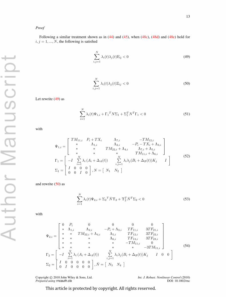
Proof

Following a similar treatment shown as in (44) and (45), when (48c), (48d) and (48e) hold fori, j = 1, ..., N , the following is satisfied

N∑i,j=1

λi(t)λj(t)Eij < 0 (49)

N∑i,j=1

λi(t)λj(t)Ξij < 0 (50)

Let rewrite (49) as

N∑i=1

λi(t)Ψ1,i + Γ1TNΣ1 + ΣT1N

TΓ1 < 0 (51)

with

Ψ1,i =

TM11,i Pi + TXi Λ7,i −TM12,i

∗ Λ1,i Λ2,i −Pi − TXi + Λ3,i

∗ ∗ TM22,i + Λ4,i Λ7,i + Λ5,i

∗ ∗ ∗ TM11,i + Λ6,i

Γ1 =

[−I

N∑i=1

λi (Ai + ∆A(t))N∑

i,j=1

λiλj(Bi + ∆B(t))Kj I

]Σ1 =

[I 0 0 00 0 I 0

], N =

[N1 N2

](52)

and rewrite (50) as

N∑i=1

λi(t)Ψ2,i + Σ2T NΥ2 + ΥT

2 NTΣ2 < 0 (53)

with

Ψ2,i =

0 Pi 0 0 0 0∗ Λ1,i Λ2,i −Pi + Λ3,i TF11,i 3TF21,i

∗ ∗ TM22,i + Λ4,i Λ5,i TF12,i 3TF22,i

∗ ∗ ∗ Λ6,i TF13,i 3TF23,i

∗ ∗ ∗ ∗ −TM11,i 0∗ ∗ ∗ ∗ ∗ −3TM11,i

Γ2 =

[−I

N∑i=1


i,j=1

λiλj(Bi + ∆B(t))Kj I 0 0

]Σ2 =

[I 0 0 0 0 00 I 0 0 0 0

], N =

[N3 N4

](54)



14

The matrix variables N1,N2,N3 and N4 are the slack variables. By finding explicit basis for thenull-space of Γ1 and Γ2 as

Γ⊥1 =

N∑i=1


i,j=1

λiλj(Bi + ∆B(t))Kj I

I 0 00 I 00 0 I

Γ⊥2 =

N∑i=1


i,j=1

λiλj(Bi + ∆B(t))Kj I 0 0

I 0 0 0 00 I 0 0 00 0 I 0 00 0 0 I 00 0 0 0 I

(55)

and applying the projection lemma, with considering P = Pi, X = Xi, X1 = X1,i, M11 =M11,i,M12 = M12,i,M22 = M22,i for i = 1, ..., N , we have

N∑i,j=1

λiλj (Πij + TΦij) = Γ⊥1T

(N∑i=1

λiΨ1,i

)Γ⊥1 (56)

and

N∑i,j=1

λiλj

Πij + TΘ TF1,i TF2,i

∗ −TM11 0∗ ∗ −3TM11

= Γ⊥2T

(N∑i=1

λiΨ2,i

)Γ⊥2 (57)

This means that the feasibility of Eq.(48c) implies the feasibility of Eq.(24c). Also the feasibilityof Eq.(48d) implies the feasibility of Eq.(24d). This completes the proof.

Remark 4The feasibility of criterion (48) implies the feasibility of the stability conditions (24) wherethe matrices P ,X ,M11,M12,M22 need to be found for all subsystems. Considering a parameterdependent functional P (λ(t)) =

∑Ni=1 λi(t)Pi implies that the LMI (24) is not affine in λi(t)

and thus the convexity is lost. Therefore, we cannot simply check the conditions at the verticesof the double-layer polytope. Decoupling between LKF matrices P , X , M11, M12, M22 and thedata matrices Ai + ∆A(t), Bi + ∆B(t), by means of introducing slack variables, allows the LMIcondition (24) to be turned into a finite set of LMIs and then robust stability with less conservativeconditions is achieved. This is a remarkable advantage of the proposed approach compared to theexisting state of the art approaches. Furthermore, in the stability analysis, the criterion (24) has animportant feature since it leads to a fairly low computational complexity due to the absence of slackvariables and the small number of decision matrices.

Remark 5It is well-known that, an LMI cab be effectively applied for a stabilization problem if thereis only one coupling between a decision matrix and the system variables. The LMI stabilitycondition (24) is not very suited for stabilization purposes due to the product terms P (Ai + ∆A(t)),(Ai + ∆A(t)

T)M11(Ai + ∆A(t)) and X(Ai + ∆A(t)). The stability analysis criterion (48) can be

efficiently solved for the stabilization problem, because by assuming all slack variables to be equal,then there is only one coupling between a decision matrix and the system variables.



15

4. CONTROLLER SYNTHESIS

In this section, we address synthesis of sampled-data PLPV controller for system in Eq.(18) usingthe results in Theorem 2. In order to improve the transient behaviour, a constrained pole placement isconsidered leading to robust controller design. Considering the performance criteria in the controllerdesign procedure is an important feature of the proposed method. Consequently, the main objectiveis to determine the feedback gain matrices Kj such that not only the inequality (48) holds but alsoadditional constraints on the location of the closed-loop poles are satisfied. To this aim, we extendedthe D-stability problem (introduced in [37]) for design of robust PLPV control with pole placementconstraints.

Lemma 6 ([37])The system matrix A is D-stable (i.e., all the poles of A lie in D) if and only if there exists asymmetric matrix Z such that D(A,Z) < 0, Z > 0, where D(A,Z) is related with the followingcharacteristic function fD(z) on the basis of the substitution

(Z,AZ,ZAT

)<=> (1, z, z):

(i) left half plane such that R(z) < −α

D = z ∈ C|fD(z) = z + z + 2α < 0 (58)

(ii) disk with center at (q, 0) and radius r:

D =

z ∈ C|fD(z) =

[−r q + zq + z −r

]< 0

(59)

(iii) conic sector centered at the origin and with inner angle 2θ:

D =

z ∈ C|fD(z) =

[sin θ (z + z) cos θ (z − z)cos θ (z − z) sin θ (z + z)

]< 0

(60)

The following theorem presents a set of LMIs for synthesis of robust pole placemen PLPVcontroller for PLPV system in (18) without considering aperiodic sampling from the states.

Theorem 3The PLVP system in (18) is D-stable if there exist a matrices Mij ∈ Rn, Lij ∈ R2n, Vij ∈ R2n

with Mij = MjiT , Lij = Lji

T , Vij = VjiT , a matrix Z ∈ Sn and matrices Yi ∈ Rn×nu such that

the following LMIs feasible for i, j = 1, ..., N

He [Ωij + Ωji + 2αZ] < Mij +Mji (61a)[−2rZ 2qZ + Ωij + Ωji∗ −2rZ

]< Lij + Lji (61b)[

sin θHe (Ωij + Ωji) cos θ(Ωij − ΩTij + Ωji − ΩTji

)∗ sin θHe (Ωij + Ωji)

]< Vij + Vji (61c) M11 · · · M1N

.... . .

...MN1 · · · MNN

< 0 ,

L11 · · · L1N

.... . .

...LN1 · · · LNN

< 0 ,

V11 · · · V1N...

. . ....

VN1 · · · VNN

< 0

(61d)

where Ωij = (Ai + ∆A(t))Z + (Bi + ∆B(t))Yj , then the control gains Kj can be reconstructed byKj = YjZ

−1.

ProofBased on Lemma 6, the pole placement constraints are satisfied if there exists Z > 0 such that

D

(N∑i=1

λi (Ai + ∆A(t)) +

N∑i,j=1

λiλj(Bi + ∆B(t))Kj , Z

)< 0 (62)



16

Therefore, the D-stability condition of (18) are given by

He [Ω (λ) + αZ] < 0 (63)

[−rZ q ∗ Z + Ω (λ)∗ −rZ

]< 0 (64)

[sin θHe (Ω (λ)) cos θ

(Ω (λ)− ΩT (λ)

)∗ sin θHe (Ω (λ))

]< 0 (65)

where

Ω (λ) =

N∑i=1

λi (Ai + ∆A(t)) +

N∑i=1

λi(Bi + ∆B(t))

N∑j=1

λjYj

N∑j=1

λjYj =

N∑j=1

λjKjZ,

Hence D-stability condition given in (63)-(65) can be assured by (61).

In the following, an efficient procedure for robust sampled-data PLPV controller synthesis forPLPV system (18) is proposed that meets the design specifications in the sampling interval whilethe aperiodic sampling period is considered as a parameter. By employing the presented results inTheorem 2 the exponential stability of the designed sampled-data controller is guaranteed.

Theorem 4Assume there exist Pi ∈ Sn+, Xi, M11,i, M22,i ∈ Sn, Yij ∈ R4n, Zij ∈ R6n with Yij = Y Tji , Zij =

ZTji and matrices N, X1,i, M12,i, F11,i, F12,i, F13,i, F21,i, F22,i, F23,i ∈ Rn×n, Yi ∈ Rn×nu withpositive scalars ε1, ε2, ε3 such that the following LMIs feasible for i, j = 1, ..., N[

M11,i M12,i

∗ M22,i

]> 0 (66a)

[I 0

]TPi[I 0

]+ T

[Xi −Xi + X1,i

∗ Xi − X1,i − XT1,i

]> 0 (66b)

Eij + Eji < Yij + Yji (66c)Ξij + Ξji < Zij + Zji (66d) Y11 · · · Y1N

.... . .

...YN1 · · · YNN

< 0 ,

Z11 · · · Z1N

.... . .

...ZN1 · · · ZNN

< 0 (66e)

Where

Eij =

TM11,i −He (N) Λ7,i Λ9,i + (Bi + ∆B(t))Yj −TM12,i +N∗ Λ8,i Λ2,i + ε1(Bi + ∆B(t))Yj −Pi − TXi + Λ3,i + ε1N∗ ∗ TM22,i + Λ4,i Λ9,i + Λ5,i

∗ ∗ ∗ TM11,i + Λ6,i



17

Ξij =

−ε2He (N) Λ10,i ε2(Bi + ∆B(t))Yj ε2N 0 0

∗ Λ11,i Λ2,i + ε3(Bi + ∆B(t))Yj −Pi + Λ3,i T F11,i 3T F21,i

∗ ∗ TM22,i + Λ4,i Λ5,i T F12,i 3T F22,i

∗ ∗ ∗ Λ6,i T F13,i 3T F23,i

∗ ∗ ∗ ∗ −TM11,i 0∗ ∗ ∗ ∗ ∗ −3TM11,i

Λ1,i = −Xi +He

(−F11,i − 3F21,i

)Λ2,i = −X1,i + Xi + F11,i − FT12,i − 3F21,i − 3FT22,i − M12,i

Λ3,i = −FT13,i + 6F21,i − 3FT23,i, Λ4,i = −Xi +He(X1,i + F12,i − 3FT22,i + M12,i

)Λ5,i = FT13,i + 6F22,i − 3FT23,i, Λ6,i = 6F23,i + 6FT23,i

Λ7,i = Pi + TXi + (Ai + ∆A(t))N, Λ8,i = Λ1,i +He (ε1 (Ai + ∆A(t))N)

Λ9,i = T(X1,i − Xi + M12,i

), Λ10,i = Pi + ε2 (Ai + ∆A(t))N

Λ11,i = Λ1,i +He (ε3 (Ai + ∆A(t))N)

Then, the sampled-data PLPV state feedback controller in Eq.(7) with vertex gains calculatedas Kj = Yj ∗N−1, exponentially stabilize the PLPV system in Eq.(18) with aperiodic samplingintervals smaller than T > 0.

ProofWe employ the stability analysis conditions presented in Eq.(48) to develop conditions for sampled-data PLPV controller design. Applying the congruent transformation diag(N,N) on Eqs.(48a) and(48b) with considering

M11,i = NTM11,iN, M12,i = NTM12,iN, M22,i = NTM22,iNPi = NTPiN, Xi = NTXiN, X1,i = NTX1,iN, N−11 = N

(67)

the LMI conditions in Eq.(66a) and Eq.(66b) obtained.Also LMI conditions in Eq.(66c) and Eq.(66d) with applying the congruent transformation

T1 = diag(N,N,N,N) and T2 = diag(N,N,N,N,N,N) on Eq.(51) and Eq.(53) respectively andconsidering

N2 = ε1N1, N3 = ε2N1, N4 = ε3N1, Yj = KjNF11,i = NTF11,iN, F12,i = NTF12,iN, F13,i = NTF13,iNF21,i = NTF21,iN, F22,i = NTF22,iN, F21,i = NTF22,iNYij = TT1 YijT1, Zij = TT2 ZijT2.

(68)

obtain. With this concludes the proof.

Remark 6We could combine the conditions of the sampled-data PLPV controller design in Theorem 4 andthe robust PLPV controller design with constrained pole placement method in Theorem 3. By doingthis, we obtained an LMI-based stabilization condition capable of achieving the pole-placementobjectives and considering sample and hold constraints (aperiodic sampling period). Consequently,the proposed method can be seen as a new approach to design sampled-data PLPV controller withimproved closed-loop transient behaviour.

5. NUMERICAL EXAMPLES

In this section, the efficiency of the proposed method is studied by three examples. In the firstexample, we show improvement in the performance of sampling interval bound by the proposedapproach for LTI system, compared with some recent state of the art input delay approaches. Thesecond example investigates the validity of the results of theorems stated in this paper for stability



18

analysis of sampled-data LPV systems. In this example, we consider a simple second order affineLPV system with a given affine LPV controller and the MASP is computed for different rates ofparameter variation. In the third example, the main application of the proposed method for sampled-data PLVP systems, has been investigated. A real world problem of balancing an inverted pendulumon a car is considered to illustrate the effectiveness of the proposed stability and design algorithmin reducing conservatism of stability analysis and improving transient behaviour of sampled-dataPLPV systems.Example 1: Consider the following well-known delay dependent stable linear system [38]:

x(t) =

[−2 00 −0.9

]x(t) +

[−1 0−1 −1

]x(tn) (69)

We use different methods to calculate the upper bound of the aperiodic sampling period thatguarantees the stability of this system. The results are presented in Table I. The MASP is usuallyused in the literature as criterion for comparing the conservativeness of stability theorems. Thebounds of the MASP are computed using the eigenvalue analysis of the corresponding transitionmatrix. Number of the scalar decision variables calculated based on Table II. The calculated valuesindicate that the proposed criteria in Theorem 1 leads to a less conservative result. Also one obtainsthat the results of Theorem 2 and Theorem 1 are same while Theorem 2 has higher computationalcomplexity.

Table I. Maximum bound on the aperiodic sampling period (Example 1).

Method Th. bounds [12] [11] [33](Theorem 2) Theorem 1 Theorem 2Tm 3.272 1.563 2.515 2.515 2.627 2.627No. of variables - 12 34 42 36 52

Table II. Numerical complexity of the different methods.

Method No. of decision variables No. of LMIs Maximum order of LMI[12] 2n2 + 2n 5 4n[11] 8n2 + n 3 4n[33] 10n2 + n 4 4nTheoream 1 8n2 + 2n 5 4nTheoream 2 12n2 + 2n 5 5n

Example 2: Consider the following LPV system.

x(t) =

[0 1

0.1 0.4 + 0.6σ(t)

]x(t) +

[01

]u(t) (70)

with |σ(t)| ≤ 1 and |σ(t)| ≤ 0.2. In [27], the following stabilizing sampled-data controller designedfor a given maximum bound on aperiodic sampling period (Tm = 400ms).

k = [−1.21 − 2.35] + [0.149 − 0.15]σ(tn) (71)

We can represent (70) accurately in PLVP form. According to (13), we have[α1(t)α1(t)

]=

[−0.5 0.50.5 0.5

]([−0.2 0.2

1 1

] [β1(t)β2(t)

]−[

01

]). (72)

Therefore, αi(t) ∈ [−0.1, 0.1] for i = 1, 2.In the following, we evaluate conservativeness of the stability conditions for different rates of

parameter variation. Table III shows maximum bound on the sampling period for different existingapproach for stability analysis of sampled-data LPV systems. It is verified that the proposed



19

Table III. Maximum bound on the aperiodic sampling period of sampled-data LPV system

Th. bounds on σ(t) 0.2 0.6 1[22] 0.39 0.38 0.36[27](P ) 0.65 0.58 0.52[27](P (σ(t))) 0.73 0.69 0.66Theoream 1 0.71 0.66 0.65Theoream 2 0.77 0.73 0.69

Radio Modem

Communication Boards

Serial Port

radio Link

( )x t ( )u t

( )ku t

( )kx t( ( ))x t t

( ( ))u t t

Figure 3. Control architecture of inverted pendulum on a car.

approach in Theorem 2 has higher performance than the loop functional [27] and a smooth LKF[22] approaches and reducing conservatism of stability.

Example 3: Consider the following equations of motion for the pendulum on a car

x1 = x2 (73)

x2 =g sin(x1)− amlx22 sin(2x1)/2− a cos(x1)u

4l/3− amlcos2(x1). (74)

where x1 denotes the angle of the pendulum from the vertical, x2 is the angular velocity, g =9.8m/s2 is the gravity, m is the mass of the pendulum, M is the mass of the cart, 2l is the length ofthe pendulum, and u is the force applied to the cart, a = 1/(m+M), m = 2kg, M = 8kg, 2l = 1mare chosen for simulation. The following polytopic quasi-LPV model of the inverted pendulum ona car systems presented in [39].

A1 =

[0 1

17.29 0

], B1 =

[0

−0.176

]A2 =

[0 1

12.63 0

], B2 =

[0

−0.077

]α1(t) =

(1− 1

1 + exp(−7[x1 − π/4])

)(1

1 + exp(−7[x1 + π/4]

)α2(t) = 1− α1(t) (75)

The sate of the inverted pendulum on a car are measured at sampling instants, tn and through a radiomodem sent to the PC. The PC computes desirable control input and sent it to inverted pendulumon a car, see Fig.(3).

We design the following controller1 with pole placement in regionsR(z) ≤ −3, and controller2without the pole placement constraints for T = 0.15 and |αi| ≤ 0.1.

controller1 = [191.31 53.11]α1(tn) + [339.98 101.23]α2(tn) (76)controller2 = [250.16 63.23]α1(tn) + [449.61 122.84]α2(tn) (77)



20

We also considered the following H∞ controller designed in [40].

K1 = [409.75 99.23], K2 = [512.91 121.79]. (78)

Fig. 4 and Fig. 5 show comparison of the response of closed loop of system for an initial conditionx1(0) = [1.2− 1]. Fig .6 shows applied control signals. We observe that designed controller1 hasthe suitable performance despite the variable sampling. The figures clearly demonstrate that in thepresence of aperiodic sampling period and despite of the uncertainties on scheduling parameters,the states tend to the origin with an acceptable settling time. Also the control signals are enoughsmooth and variation of sampling is not effective.

Figure 4. Comparison of the response of system under the controller obtained by Theorem 4.

The criteria proposed in Theorem 2 is applied to identify the upper bounded of aperiodic samplingperiod of the PLPV model of inverted pendulum on a car with different rate of parameter variationfor three different controllers. Table IV shows the results. This comparison shows the advantageousof the proposed sampled-data PLPV control design scheme for networked control systems.

Table IV. Maximum bound on the aperiodic sampling period of sampled-data LPV system

Th. bounds on αi(t) 0.1 0.3 1controller1 0.168 0.161 0.147controller2 0.202 0.194 0.175Liu Xiaodonga [40] 0.108 0.105 0.101

6. CONCLUSION

In this paper we proposed a new methodology for exponential stability analysis and design ofthe closed loop sampled-data PLPV systems with aperiodic sampling. The proposed method hasthree important features: (i) new form of discrete LKF with the Wirtingers inequality was proposedthat provides less conservative stability analysis condition of sampled-data PLPV systems ratherthan existing methods, (ii) double-layer description utilized to model inequality among real andsampled parameters which reduced the complexity and in combination with the proposed stability



21

Figure 5. Comparison of the response of system under the controller obtained by Theorem 4.

Figure 6. Control signal with T = 0.15.

conditions has suitable performance in MASP computations, and (iii) a sampled-data polytopicLPV controller was synthesized regarding the aperiodic sampling and the proposed pole placementtechnique provided a viable control strategy. The effectiveness of the approach was verified bymeans of numerical simulations that illustrated a significant robustness for aperiodic samplingwithout performance degrading. The computational complexity of the proposed approach for largesystems with large numbers of scheduling parameters is an important issue need to be considered.Finally, it is noted that the complexity reduction of the proposed method and extending it to theoutput feedback control problems is our current ongoing work. To this aim, the idea is to use lessconservative available tools rather than the Wirtinger-based inequalities (see e.g. [41, 42, 43]) toprovide a smaller bounding gap.



22

REFERENCES

1. Hespanha JP, Naghshtabrizi P, Xu Y. A survey of recent results in networked control systems. Proc-IEEE 2007;95(1):138.

2. Yang F, Zhang H, Liu Z, Li R. Delay-dependent resilient-robust stabilisation of uncertain networked control systemswith variable sampling intervals. International Journal of Systems Science 2014; 45(3):497–508.

3. Orihuela L, Millan P, Vivas C, Rubio FR. Event-based H2/H∞ controllers for networked control systems.International Journal of Control 2014; 87(12):2488–2498.

4. Park MJ, Kwon OM, Seuret A. Weighted consensus protocols design based on network centrality for multi-agentsystems with sampled-data. IEEE Transactions on Automatic Control 2017; 62(6):2916–2922.

5. Yamamoto Y. A function space approach to sampled data control systems and tracking problems. IEEE Transactionson Automatic Control 1994; 39(4):703–713.

6. Mirkin L, et al.. Some remarks on the use of time-varying delay to model sample-and-hold circuits. IEEETransactions on Automatic Control 2007; 52(6):1109.

7. Naghshtabrizi P, Hespanha JP, Teel AR. Exponential stability of impulsive systems with application to uncertainsampled-data systems. Systems & Control Letters 2008; 57(5):378–385.

8. van de Wouw N, Naghshtabrizi P, Cloosterman M, Hespanha JP. Tracking control for sampled-data systems withuncertain time-varying sampling intervals and delays. International Journal of Robust and Nonlinear Control 2010;20(4):387–411.

9. Seuret A. A novel stability analysis of linear systems under asynchronous samplings. Automatica 2012; 48(1):177–182.

10. Seuret A, Briat C. Stability analysis of uncertain sampled-data systems with incremental delay using looped-functionals. Automatica 2015; 55:274–278.

11. Fridman E. A refined input delay approach to sampled-data control. Automatica 2010; 46(2):421–427.12. Liu K, Fridman E. Wirtingers inequality and Lyapunov-based sampled-data stabilization. Automatica 2012;

48(1):102–108.13. Mazenc F, Malisoff M, Dinh TN. Robustness of nonlinear systems with respect to delay and sampling of the

controls. Automatica 2013; 49(6):1925–1931.14. Karafyllis I, Kravaris C. Global stability results for systems under sampled-data control. International Journal of

Robust and Nonlinear Control 2009; 19(10):1105–1128.15. Nesic D, Teel AR, Carnevale D. Explicit computation of the sampling period in emulation of controllers for

nonlinear sampled-data systems. IEEE Transactions on Automatic Control 2009; 54(3):619–624.16. Lee S, Park M, Kwon O, Sakthivel R. Synchronization of lur’e systems via stochastic reliable sampled-data

controller. Journal of the Franklin Institute 2017; 354(5):2437–2460.17. Lee S, Park M, Kwon O, Sakthivel R. Advanced sampled-data synchronization control for complex dynamical

networks with coupling time-varying delays. Information Sciences 2017; .18. Hoffmann C, Werner H. A survey of linear parameter-varying control applications validated by experiments or

high-fidelity simulations. IEEE Transactions on Control Systems Technology 2015; 23(2):416–433.19. Henry D, Cieslak J, Zolghadri A, Efimov D. H∞ LPV solutions for fault detection of aircraft actuator faults:

Bridging the gap between theory and practice. International Journal of Robust and Nonlinear Control 2015;25(5):649–672.

20. Tan K, Grigoriadis KM. State-feedback control of LPV sampled-data systems. Mathematical Problems inEngineering 2000; 6(2-3):145–170.

21. Tan K, Grigoriadis KM, Wu F. Output-feedback control of LPV sampled-data systems. International Journal ofControl 2002; 75(4):252–264.

22. Ramezanifar A, Mohammadpour J, Grigoriadis K. Sampled-data control of LPV systems using input delayapproach. IEEE 51st Annual Conference on Decision and Control (CDC), IEEE, 2012; 6303–6308.

23. Ramezanifar A, Mohammadpour J, Grigoriadis KM. Sampled-data control of linear parameter varying time-delaysystems using state feedback. American Control Conference (ACC), IEEE, 2013; 6847–6852.

24. Ramezanifar A, Mohammadpour J, Grigoriadis KM. Output-feedback sampled-data control design for linearparameter-varying systems with delay. International Journal of Control 2014; 87(12):2431–2445.

25. Shi T, Su H. Sampled-data mpc for LPV systems with input saturation. IET Control Theory & Applications 2014;8(17):1781–1788.

26. Lee S, Kwon O. Quantised mpc for LPV systems by using new lyapunov–krasovskii functional. IET Control Theory& Applications 2016; 11(3):439–445.

27. Da Silva JG, Moraes V, Flores J, Palmeira A. Sampled-data LPV control: a looped functional approach. IFAC-PapersOnLine 2015; 48(26):19–24.

28. Takagi T, Sugeno M. Fuzzy identification of systems and its applications to modeling and control. IEEE transactionson systems, man, and cybernetics 1985; (1):116–132.

29. Boustany N. Unified algebraic approach to linear control design. re skelton et al. APPLIED MECHANICSREVIEWS 1998; 51:B89–B89.

30. Xie L, de Souza Carlos E. Robust h/sub infinity/control for linear systems with norm-bounded time-varyinguncertainty. IEEE Transactions on Automatic Control 1992; 37(8):1188–1191.

31. Seuret A, Gouaisbaut F. Wirtinger-based integral inequality: application to time-delay systems. Automatica 2013;49(9):2860–2866.

32. Gao H, Sun W, Shi P. Robust sampled-data H∞ control for vehicle active suspension systems. IEEE Transactionson Control Systems Technology 2010; 18(1):238–245.

33. Zhang CK, Jiang L, He Y, Wu H, Wu M. Stability analysis for control systems with aperiodically sampled datausing an augmented lyapunov functional method. IET Control Theory & Applications 2013; 7(9):1219–1226.

34. Xu S, Sun G, Sun W. Fuzzy logic based fault-tolerant attitude control for nonlinear flexible spacecraft with sampled-data input. Journal of the Franklin Institute 2017; 354(5):2125–2156.



23

35. Xu S, Sun G, Sun W. Reliable sampled-data vibration control for uncertain flexible spacecraft with frequency rangelimitation. Nonlinear Dynamics 2016; 86(2):1117–1135.

36. Gahinet P, Apkarian P. A linear matrix inequality approach to H∞ control. International journal of robust andnonlinear control 1994; 4(4):421–448.

37. Chilali M, Gahinet P. H∞ design with pole placement constraints: an LMI approach. IEEE Transactions onautomatic control 1996; 41(3):358–367.

38. Kao CY, Rantzer A. Stability analysis of systems with uncertain time-varying delays. Automatica 2007; 43(6):959–970.

39. Cao SG, Rees NW, Feng G. Stability analysis and design for a class of continuous-time fuzzy control systems.International Journal of Control 1996; 64(6):1069–1087.

40. Xiaodong L, Qingling Z. New approaches to H∞ controller designs based on fuzzy observers for TS fuzzy systemsvia LMI. Automatica 2003; 39(9):1571–1582.

41. Zhang CK, He Y, Jiang L, Wu M, Zeng HB. Stability analysis of systems with time-varying delay via relaxedintegral inequalities. Systems & Control Letters 2016; 92:52–61.

42. Liu K, Seuret A, Xia Y. Stability analysis of systems with time-varying delays via the second-order bessel–legendreinequality. Automatica 2017; 76:138–142.

43. Zhang CK, He Y, Jiang L, Wu M, Wang QG. An extended reciprocally convex matrix inequality for stabilityanalysis of systems with time-varying delay. Automatica 2017; 85:481–485.



Minerva Access is the Institutional Repository of The University of Melbourne

Author/s:Hooshmandi, K;Bayat, F;Jahed-Motlagh, MR;Jalali, AA

Title:Stability analysis and design of nonlinear sampled-data systems under aperiodic samplings

Date:2018-05-10

Citation:Hooshmandi, K., Bayat, F., Jahed-Motlagh, M. R. & Jalali, A. A. (2018). Stability analysis anddesign of nonlinear sampled-data systems under aperiodic samplings. International Journalof Robust and Nonlinear Control, 28 (7), pp.2679-2699. https://doi.org/10.1002/rnc.4043.

Persistent Link:http://hdl.handle.net/11343/283554

http://hdl.handle.net/11343/283554

Stability Analysis and Design of Nonlinear Sampled-Data ...

Documents

Transcript of Stability Analysis and Design of Nonlinear Sampled-Data ...