
Sst from space
52
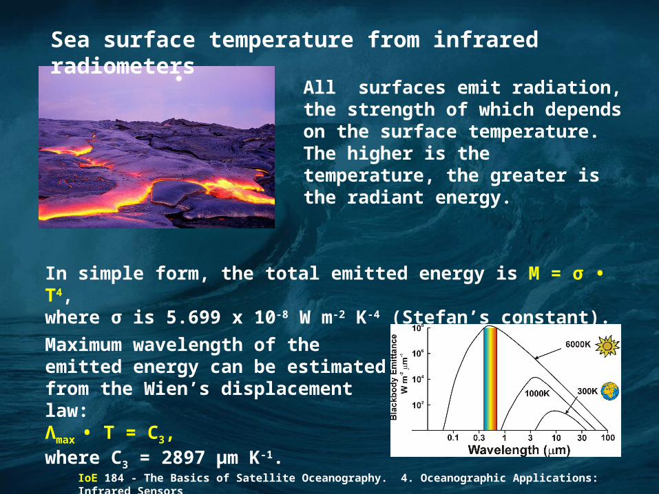
IoE 184 - The Basics of Satellite Oceanography. 4. Oceanographic Applications: Infrared Sensors Sea surface temperature from infrared radiometers All surfaces emit radiation, the strength of which depends on the surface temperature. The higher is the temperature, the greater is the radiant energy. In simple form, the total emitted energy is M = σ • T 4 , where σ is 5.699 x 10 -8 W m -2 K -4 (Stefan’s constant). Maximum wavelength of the emitted energy can be estimated from the Wien’s displacement law: Λ max • T = C 3 , where C 3 = 2897 μm K -1 .
-
Upload
nunung-aziizah -
Category
Education
-
view
45 -
download
0
Transcript of Sst from space
IoE 184 - The Basics of Satellite Oceanography. 4. Oceanographic Applications: Infrared Sensors
Sea surface temperature from infrared radiometers
All surfaces emit radiation, the strength of which depends on the surface temperature. The higher is the temperature, the greater is the radiant energy.
In simple form, the total emitted energy is M = σ • T4, where σ is 5.699 x 10⁻⁸ W m-2 K-4 (Stefan’s constant).
Maximum wavelength of the emitted energy can be estimated from the Wien’s displacement law:Λmax
• T = C3, where C3 = 2897 μm K-1.

IoE 184 - The Basics of Satellite Oceanography. 4. Oceanographic Applications: Infrared Sensors
Sea surface temperature from infrared radiometers
In practice, the measured brightness temperature differs from the actual temperature of the observed surface because of non-unit emissivity and the effect of the intervening atmosphere.
For infrared (IR) radiation the emissivity (i.e., the ratio between real exitance and a perfect emitter at this temperature) of sea surface is between 0.98 and 0.99.
The brightness temperature of the radiation is defined as the tempe-rature of the black body which would emit the measured radiance.
The brightness temperature: a descriptive measure of radiation in terms of the temperature of a hypothetical blackbody emitting an identical amount of radiation at the same wavelength.
IoE 184 - The Basics of Satellite Oceanography. 4. Oceanographic Applications: Infrared Sensors
Sea surface temperature from infrared radiometers
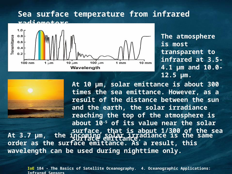
At 10 μm, solar emittance is about 300 times the sea emittance. However, as a result of the distance between the sun and the earth, the solar irradiance reaching the top of the atmosphere is about 10-5 of its value near the solar surface, that is about 1/300 of the sea surface emittance.
The atmosphere is most transparent to infrared at 3.5-4.1 μm and 10.0-12.5 μm.
At 3.7 μm, the incoming solar irradiance is the same order as the surface emittance. As a result, this wavelength can be used during nighttime only.
Sea surface temperature from infrared radiometers
IoE 184 - The Basics of Satellite Oceanography. 4. Oceanographic Applications: Infrared Sensors
For IR sensor calibration, a target of known temperature is used. This temperature is measured and transmitted to ground receiving station along with the signal measured by the IR sensor.
Atmospheric correction is based on multispectral approach, when the differences between brightness temperatures measured at different wavelengths are used to estimate the contribution of the atmosphere to the signal (more detail later, in AVHRR section).
For cloud detection, the thermal and near-infrared waveband thresholds are used, as well as different spatial coherency tests.

IoE 184 - The Basics of Satellite Oceanography. 4. Oceanographic Applications: Infrared Sensors
Sea surface temperature from infrared radiometersInterpretation of Sea Surface Temperature
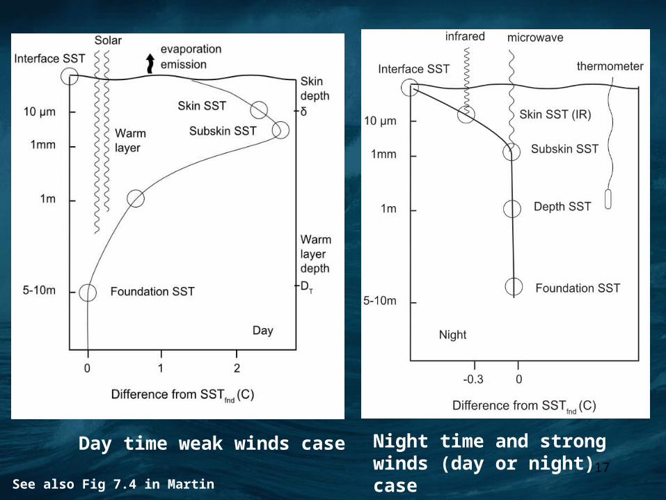
The actual thickens of the layer whose temperature is remotely sensed varies between 3 and 14 m. It is called skin SST and written Tskin or sometimes SSST.
At the same time, the measured in situ SST (called also bulk SST) corresponds to at least few centimeters or more, depending on waves. The SST measurements on buoys may be anything between 0.5 and 3 m deep.
Three physical effects may increase the difference between skin and bulk SSTs:
1) Diurnal thermocline;2) Thermal skin layer effect;3) The presence of surface film.

IoE 184 - The Basics of Satellite Oceanography. 4. Oceanographic Applications: Infrared Sensors
Sea surface temperature from infrared radiometersInterpretation of Sea Surface Temperature
Diurnal thermocline
As a result of insolation, daytime temperature in the upper layer of up to 50 cm can differ from deeper layers as much as 4C.
Since open skies are part of the requirement of diurnal warming, there is a higher probability of daytime satellite observations encountering diurnal warming events.
To control this effect, we should analyze the differences between day and night satellite SST observations.
The bulk SST (i.e., the parameter we are measuring) is invariant over the diurnal cycle.
IoE 184 - The Basics of Satellite Oceanography. 4. Oceanographic Applications: Infrared Sensors
Sea surface temperature from infrared radiometersInterpretation of Sea Surface Temperature
Diurnal thermocline
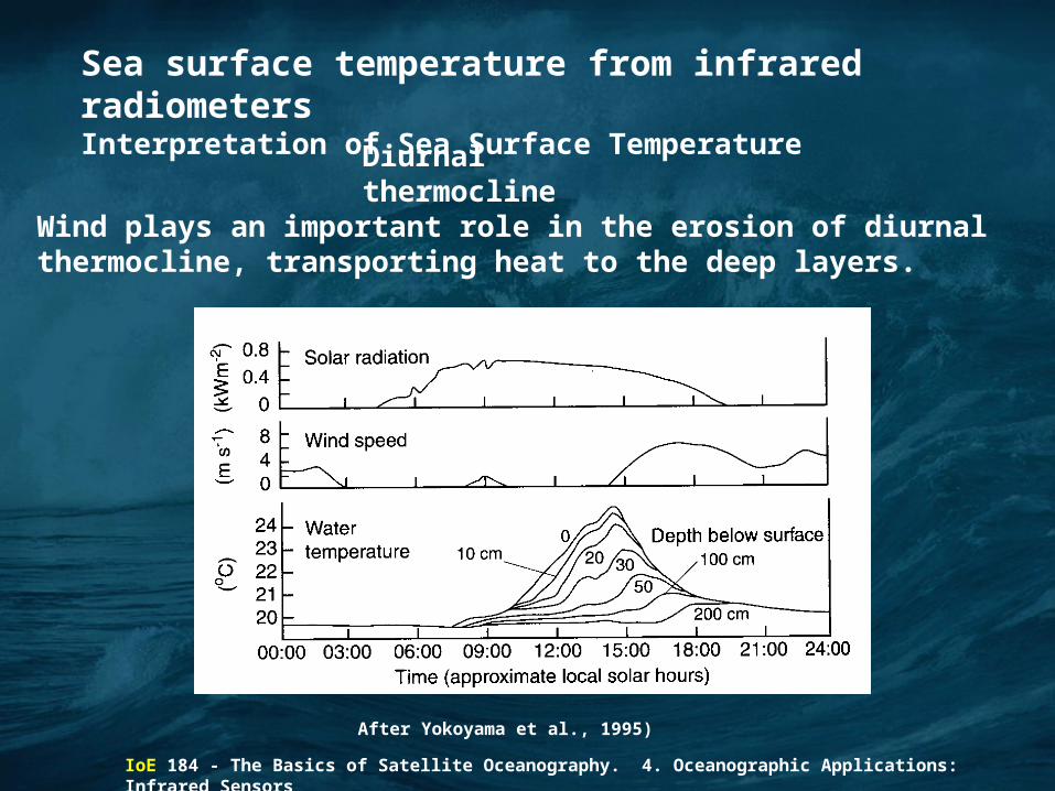
Wind plays an important role in the erosion of diurnal thermocline, transporting heat to the deep layers.
After Yokoyama et al., 1995)
IoE 184 - The Basics of Satellite Oceanography. 4. Oceanographic Applications: Infrared Sensors
Sea surface temperature from infrared radiometersInterpretation of Sea Surface Temperature
The thermal skin layer of the ocean surface
Heat flux from ocean surface to the atmosphere results in decrease of the skin temperature.
This effect is observed during both day and night.
The difference between the skin and the sub-skin temperature is typically –0.17ºC at wind speed >5 m s-1. At lower wind speeds, the picture is more complex, resulting from heat flux, which is different during day and night, humidity, swell, etc.
The skin layer is very robust. Experiments show that if the surface is completely broken and the skin is destroyed, for example by breaking wave, the skin layer reforms again in a few seconds.
IoE 184 - The Basics of Satellite Oceanography. 4. Oceanographic Applications: Infrared Sensors
Sea surface temperature from infrared radiometersInterpretation of Sea Surface Temperature
Effect of surface film
Surface film may be a naturally produced organic material or oil from shipping.
When the slick is thicker than a single layer of molecules, the emitted radiance and the resulting brightness temperature are lower.
A surface slick affects the thermal structure of the near-surface, inhibiting wind mixing and increasing diurnal thermocline. The slick also reduces evaporation. Moreover, a thick oil slick absorbs solar radiation effectively and becomes warmer than the underlying sea water.
With such a variety of opposing effects, it is not possible to predict whether the observed radiation temperature will be reduced or increased by a slick.

10

11

13
Ocean
Troposphere
Stratosphere
clouds
T
TS
Tb
sun glint
volcanic aerosols
tropospheric aerosols
sensor
Emitted surface radiance
upwelled atmospheric radiance
water vapor
buoy

14
10-12 m 3.5-4.1 m
Relative atmospheric transmission plotted vs. decreasing wavelength
p18

15
Relative atmospheric transmission plotted vs. increasing wavelength
10-12 m3.5-4.1 m

16wavelength
Sensitivity of brightness to change in blackbody temperature
brightness of 300K blackbody
Brightness temperature difference due to atmosphere
3.5 μm 10 μm 12 μm
17
Night time and strong winds (day or night) case
Day time weak winds case
See also Fig 7.4 in Martin
IoE 184 - The Basics of Satellite Oceanography. 4. Oceanographic Applications: Infrared Sensors
Sea surface temperature from infrared radiometers
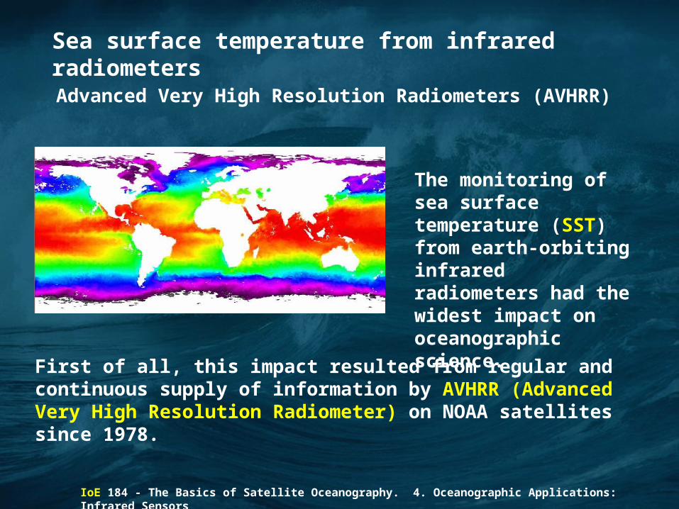
The monitoring of sea surface temperature (SST) from earth-orbiting infrared radiometers had the widest impact on oceanographic science.
First of all, this impact resulted from regular and continuous supply of information by AVHRR (Advanced Very High Resolution Radiometer) on NOAA satellites since 1978.
Advanced Very High Resolution Radiometers (AVHRR)

IoE 184 - The Basics of Satellite Oceanography. 4. Oceanographic Applications: Infrared Sensors
Sea surface temperature from infrared radiometers
VHRR (Very High Resolution Radiometer) used before had just one visible and one infrared channel.
AVHRR (Advanced Very High Resolution Radiometer) was first mounted on TIROS-N (Television Infrared Observation Satellite) in 1978.
NOAA-11
The satellites of NOAA series are near-polar sun-synchronous satellites.

IoE 184 - The Basics of Satellite Oceanography. 4. Oceanographic Applications: Infrared Sensors
Sea surface temperature from infrared radiometers
Temporal coverage of NOAA satellites with AVHRR
Satellite Number
Launch Date
Ascending Node
Descending Node
Service Dates
TIROS-N 10/13/78 1500 0300 10/19/7801/30/80
NOAA-6 06/27/79 1930 0730 06/27/7911/16/86
NOAA-7 06/23/81 1430 0230 08/24/8106/07/86
NOAA-8 03/28/83 1930 0730 05/03/8310/31/85
NOAA-9 12/12/84 1420 0220 02/25/8505/11/94
NOAA-10 09/17/86 1930 0730 11/17/86Present
NOAA-11 09/24/91 1340 0140 09/24/9109/13/94

IoE 184 - The Basics of Satellite Oceanography. 4. Oceanographic Applications: Infrared Sensors
Temporal coverage of NOAA satellites with AVHRR
Satellite Number
Launch Date
Ascending Node
Descending Node
Service Dates
NOAA-12 05/14/91 1930 0730 05/14/9112/15/94
NOAA-13 08/09/93 1430 0230 Failure
NOAA-14 12/30/94 1930 0730 12/30/9405/23/07
NOAA-15 05/13/98 1420 0220 05/13/98Present
NOAA-16 09/21/00 1930 0730 09/21/00Present
NOAA-17 06/24/02 1930 0730 06/24/02Present
NOAA-18 08/20/05 08/30/05Present
NOAA-19 02/06/09 06/02/09Present

IoE 184 - The Basics of Satellite Oceanography. 4. Oceanographic Applications: Infrared Sensors
Sea surface temperature from infrared radiometers
Sensor characteristics
Band SatellitesNOAA-6,8,10:
SatellitesNOAA-
7,9,11,12,14
SatellitesNOAA,15,16,
17,18,19
IFOV
1 0.58 - 0.68 0.58 - 0.68 0.58-0.68 1.39
2 0.725 - 1.10 0.725 - 1.10 0.73-0.98 1.41
3 3.55 - 3.93 3.55 - 3.93 1.58-1.633.54-3.87
1.51
4 10.50 - 11.50 10.3 - 11.3 10.3-11.3 1.41
5 band 4 repeated 11.5 - 12.5 11.5-12.4 1.30
(micrometers) (micrometers) (micrometers) (milli-radians)

IoE 184 - The Basics of Satellite Oceanography. 4. Oceanographic Applications: Infrared Sensors
Sea surface temperature from infrared radiometers
Sensor characteristics
The scanner has an IFOV of approximately 1.3 mrads and a cross-track scan of ±55.4º. With a nominal height of 833 km the ground FOV in nadir is 1.1 km and the swath width about 2500 km.
The orbit period is about 102 min and 14 orbits are completed per day.
The swath of adjacent orbits overlap, ensuring that the whole Earth surface is viewed at least twice a day, once from the ascending (daylight) passes and once from the descending (night) overpasses.

IoE 184 - The Basics of Satellite Oceanography. 4. Oceanographic Applications: Infrared Sensors
Sea surface temperature from infrared radiometers
The ratio between near-infrared and infrared wavebands, called Normalized Digital Vegetation Index (NDVI) is a wide-used method of the analysis of land vegetation.
IoE 184 - The Basics of Satellite Oceanography. 4. Oceanographic Applications: Infrared Sensors
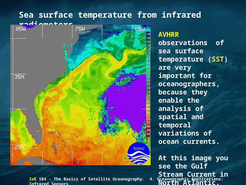
Sea surface temperature from infrared radiometers
AVHRR observations of sea surface temperature (SST) are very important for oceanographers, because they enable the analysis of spatial and temporal variations of ocean currents.
At this image you see the Gulf Stream Current in North Atlantic.

IoE 184 - The Basics of Satellite Oceanography. 4. Oceanographic Applications: Infrared Sensors
Sea surface temperature from infrared radiometers
AVHRR data are acquired in three formats:
High Resolution Picture Transmission (HRPT)
HRPT data are full resolution image data transmitted to a ground station as they are collected.
Local Area Coverage (LAC)
LAC are also full resolution data, but recorded with an on-board tape recorder for subsequent transmission during a station overpass.
Global Area Coverage (GAC)
GAC data provide daily subsampled global coverage recorded on the tape recorders and then transmitted to a ground station.

IoE 184 - The Basics of Satellite Oceanography. 4. Oceanographic Applications: Infrared Sensors
Sea surface temperature from infrared radiometers
The data are collected in several scientific centers:
EROS - Earth Resources Observation Systems data center;
EDC - Earth Resources Observation Systems Data Center;
NOAA/NESDIS - National Environmental Satellite, Data and Information Service of National Oceanic and Atmospheric Administration;
And some others.
IoE 184 - The Basics of Satellite Oceanography. 4. Oceanographic Applications: Infrared Sensors
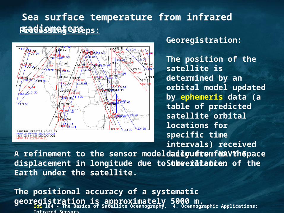
Sea surface temperature from infrared radiometersProcessing steps:
Georegistration:
The position of the satellite is determined by an orbital model updated by ephemeris data (a table of predicted satellite orbital locations for specific time intervals) received daily from NAVY Space Surveillance.
A refinement to the sensor model accounts for the displacement in longitude due to the rotation of the Earth under the satellite.
The positional accuracy of a systematic georegistration is approximately 5000 m.
IoE 184 - The Basics of Satellite Oceanography. 4. Oceanographic Applications: Infrared Sensors
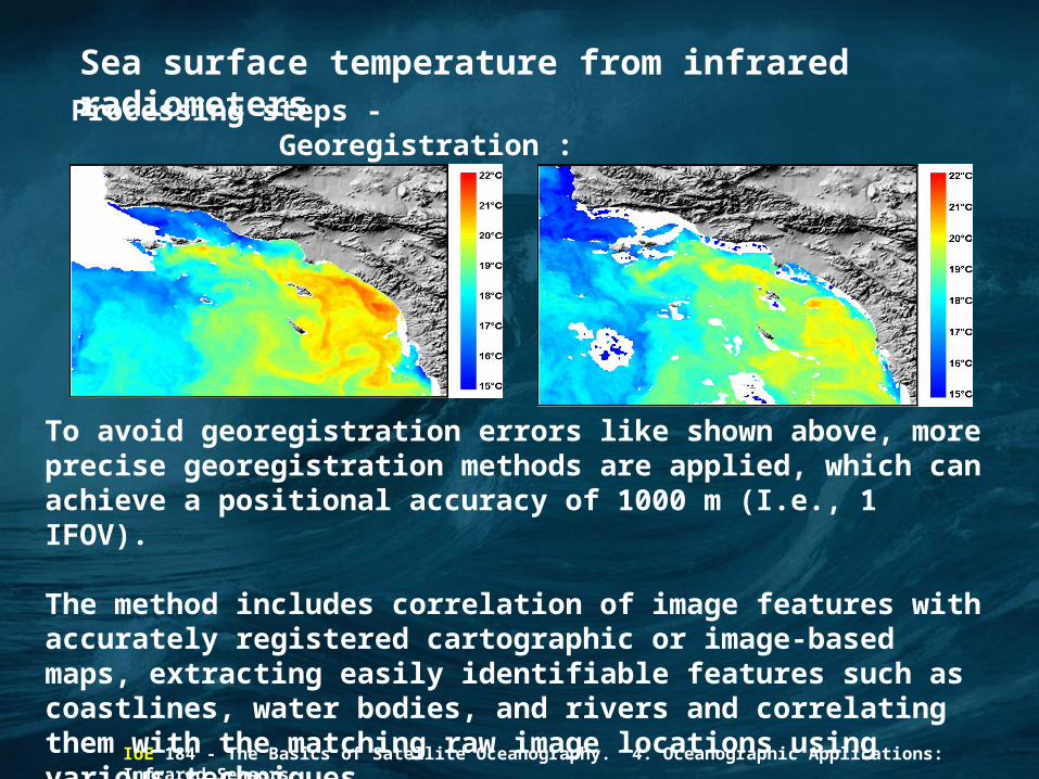
Sea surface temperature from infrared radiometersProcessing steps - Georegistration :
To avoid georegistration errors like shown above, more precise georegistration methods are applied, which can achieve a positional accuracy of 1000 m (I.e., 1 IFOV).
The method includes correlation of image features with accurately registered cartographic or image-based maps, extracting easily identifiable features such as coastlines, water bodies, and rivers and correlating them with the matching raw image locations using various techniques.

IoE 184 - The Basics of Satellite Oceanography. 4. Oceanographic Applications: Infrared Sensors
Sea surface temperature from infrared radiometersProcessing steps - Georegistration :
IoE 184 - The Basics of Satellite Oceanography. 4. Oceanographic Applications: Infrared Sensors
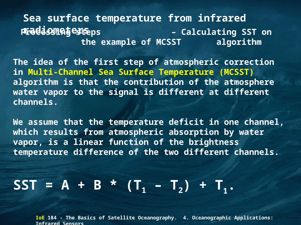
Sea surface temperature from infrared radiometersProcessing steps – Calculating SST on the
example of MCSST algorithm
The idea of the first step of atmospheric correction in Multi-Channel Sea Surface Temperature (MCSST) algorithm is that the contribution of the atmosphere water vapor to the signal is different at different channels.
We assume that the temperature deficit in one channel, which results from atmospheric absorption by water vapor, is a linear function of the brightness temperature difference of the two different channels.
SST = A + B * (T1 – T2) + T1.

IoE 184 - The Basics of Satellite Oceanography. 4. Oceanographic Applications: Infrared Sensors
Sea surface temperature from infrared radiometersProcessing steps – Calculating SST on the
example of MCSST algorithm
During daytime observations the channels 11 and 12 µm are used:
SST = 1.0346 * T11 + 2.5779 * (T11-T12) - 283.21;
During nighttime we can also use the channel 3.7 µm, which during daytime is contaminated with sunlight:
SST1 = 1.5018 * T3.7 - 0.4930 * T11 - 273.34;
SST2 = 3.6139 * T11 - 2.5789 * T12 - 283.18;
SST3 = 1.0170 * T11 + 0.9694 * (T3.7 - T12) - 276.58; (SST in degrees Celsius, T in degrees Kelvin).

IoE 184 - The Basics of Satellite Oceanography. 4. Oceanographic Applications: Infrared Sensors
Sea surface temperature from infrared radiometersProcessing steps – Calculating SST on the
example of MCSST algorithm
Atmospheric correction:
1. Visible or IR reflectance test (during daytime only):
The reflectance of the cloud-free ocean as measured at a satellite is generally less than 10%, whereas the reflectance of the most clouds is greater than 50%.

IoE 184 - The Basics of Satellite Oceanography. 4. Oceanographic Applications: Infrared Sensors
Sea surface temperature from infrared radiometersProcessing steps – Calculating SST on the
example of MCSST algorithm
Atmospheric correction:
2. Uniformity test Threshold of the variation of measurement values from adjacent cloud-free field of view is set to be slightly in excess of instrumental noise. With partially cloud-filled fields of view, the variations are generally larger.

IoE 184 - The Basics of Satellite Oceanography. 4. Oceanographic Applications: Infrared Sensors
Sea surface temperature from infrared radiometersProcessing steps – Calculating SST on the
example of MCSST algorithm
Atmospheric correction:
3. Channel intercomparison test. At night three independent measures of SST can be obtained from different channels:
SST1 = 1.5018 * T3.7 - 0.4930 * T11 - 273.34;
SST2 = 3.6139 * T11 - 2.5789 * T12 - 283.18;
SST3 = 1.0170 * T11 + 0.9694 * (T3.7 - T12) - 276.58;
When the contribution of the atmosphere is too strong, the difference between SST1, SST2 and SST3 exceeds the assumed threshold and the resulting SST is marked as invalid.

IoE 184 - The Basics of Satellite Oceanography. 4. Oceanographic Applications: Infrared Sensors
Sea surface temperature from infrared radiometersProcessing steps – Calculating SST on the
example of MCSST algorithm
Atmospheric correction:
4. The retrieved SSTs are compared with climatology and with SSTs retrieved using alternative algorithms.
First, the SST is subject to “unreasonableness” test, i.e., SST must be within the range from 2ºC to +35ºC.
Second, the retrieved SST must pass a climatology test, meaning that it must agree with monthly climatology at its location within 10ºC.
As a result, 80–90% of AVHRR pixels are considered cloudy.

IoE 184 - The Basics of Satellite Oceanography. 4. Oceanographic Applications: Infrared Sensors
Sea surface temperature from infrared radiometers
The AVHRR data obtained during one week contain many areas where no data was collected due to cloud cover.
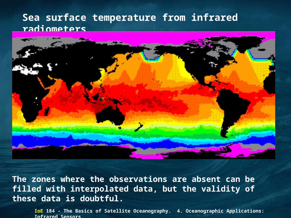
IoE 184 - The Basics of Satellite Oceanography. 4. Oceanographic Applications: Infrared Sensors
Sea surface temperature from infrared radiometers
The zones where the observations are absent can be filled with interpolated data, but the validity of these data is doubtful.

IoE 184 - The Basics of Satellite Oceanography. 4. Oceanographic Applications: Infrared Sensors
Sea surface temperature from infrared radiometers
During recent years AVHRR data are step-by-step reanalyzed within “Pathfinder” Project at NASA Jet Propulsion Laboratory (JPL) using sophisticated algorithm bases on numerous contact measurements of sea surface temperature.

IoE 184 - The Basics of Satellite Oceanography. 4. Oceanographic Applications: Infrared Sensors
Sea surface temperature from infrared radiometers
Sea Surface Temperatures obtained during daytime and nighttime are essentially different and should not be compared at the series of images. This difference results from not only the daytime thermocline, but from different algorithms also.
IoE 184 - The Basics of Satellite Oceanography. 4. Oceanographic Applications: Infrared Sensors
Sea surface temperature from infrared radiometers
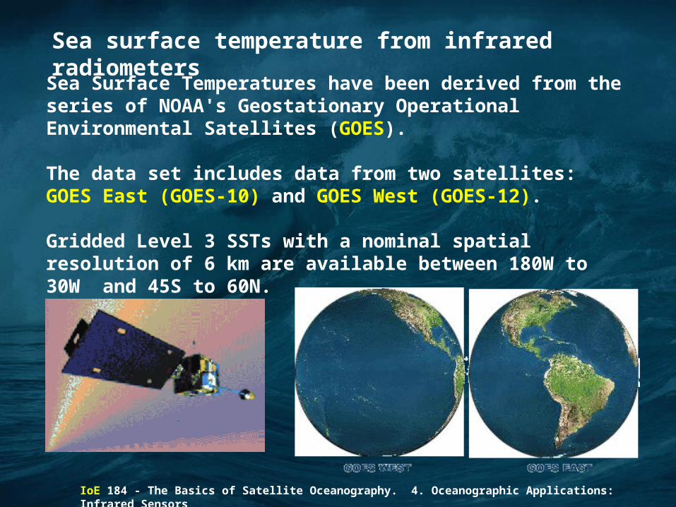
Sea Surface Temperatures have been derived from the series of NOAA's Geostationary Operational Environmental Satellites (GOES).
The data set includes data from two satellites: GOES East (GOES-10) and GOES West (GOES-12).
Gridded Level 3 SSTs with a nominal spatial resolution of 6 km are available between 180W to 30W and 45S to 60N.

IoE 184 - The Basics of Satellite Oceanography. 4. Oceanographic Applications: Infrared Sensors
Sea surface temperature from infrared radiometers
Each satellite is equipped with GOES Imager radiometer which collects information on 5 channels (1 visible and 4 infrared).
The scans are every hour, IFOV is 4 km.
Brightness temperatures from the 5-channel instrument are regressed against buoy data to derive a set of coefficients. These coefficients are then used to convert the brightness temperatures to an SST measurement. The theory itself is very similar to the non-linear algorithm used to process AVHRR-derived SSTs.

IoE 184 - The Basics of Satellite Oceanography. 4. Oceanographic Applications: Infrared Sensors
Sea surface temperature from infrared radiometers

IoE 184 - The Basics of Satellite Oceanography. 4. Oceanographic Applications: Infrared Sensors
Sea surface temperature from infrared radiometers
CoastWatch sea surface temperature data source and software
http://coastwatch.pfel.noaa.gov/
The CoastWatch Internet site is an example of satellite data source.
This site provides AVHRR SST data along the West Coast of USA during few recent months.
SeaDAS Training ~ NASA Ocean Biology Processing Group
45
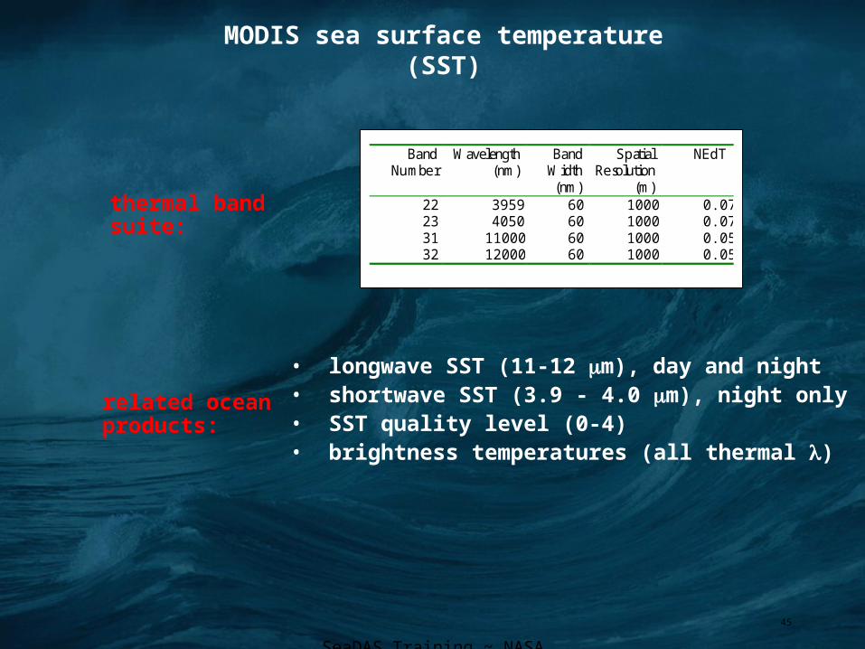
MODIS sea surface temperature (SST)
Band Number
Wavelength (nm)
Band Width
(nm)
Spatial Resolution
(m)
NEdT
22 3959 60 1000 0.07 23 4050 60 1000 0.07 31 11000 60 1000 0.05 32 12000 60 1000 0.05
• longwave SST (11-12 m), day and night• shortwave SST (3.9 - 4.0 m), night only• SST quality level (0-4)• brightness temperatures (all thermal )
thermal band suite:
related ocean products:

SeaDAS Training ~ NASA Ocean Biology Processing Group
46
Level-2 SST processing
(1) convert observed radiances to brightness temperatures (BTs)
(2) apply empirical algorithm to relate brightness temperature in 2 wavelengths to SST
sst = a0 + a1*BT1 + a2*(BT2-BT1) + a3*(1.0/-1.0)
(3) assess quality (0=best, 4=not computed)
* e.g., cloud or residual water vapor contamination
* no specific “cloud mask”

SeaDAS Training ~ NASA Ocean Biology Processing Group
47
Daytime SST products
longwave SST shortwave SST
Sun glintcloud
SeaDAS Training ~ NASA Ocean Biology Processing Group
48
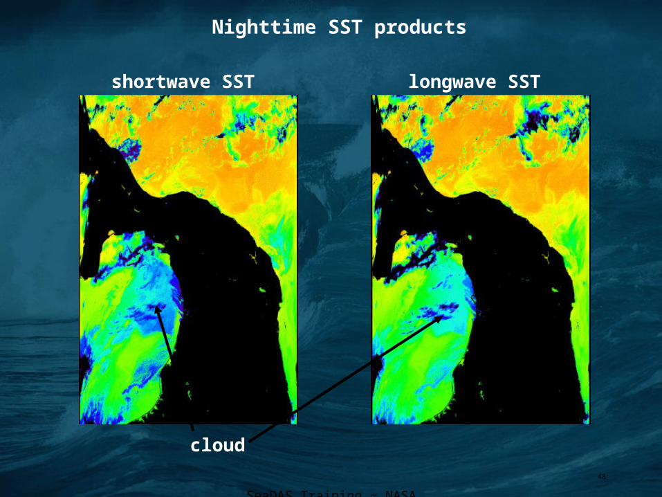
Nighttime SST products
longwave SSTshortwave SST
Cloud
cloud

SeaDAS Training ~ NASA Ocean Biology Processing Group
49
SST quality levels
QL=0
QL=1
QL=2
QL=4
QL=3
shortwave SST shortwave SST QL

SeaDAS Training ~ NASA Ocean Biology Processing Group
50
SST quality tests
SST quality tests
SST quality levels
SeaDAS Training ~ NASA Ocean Biology Processing Group
51
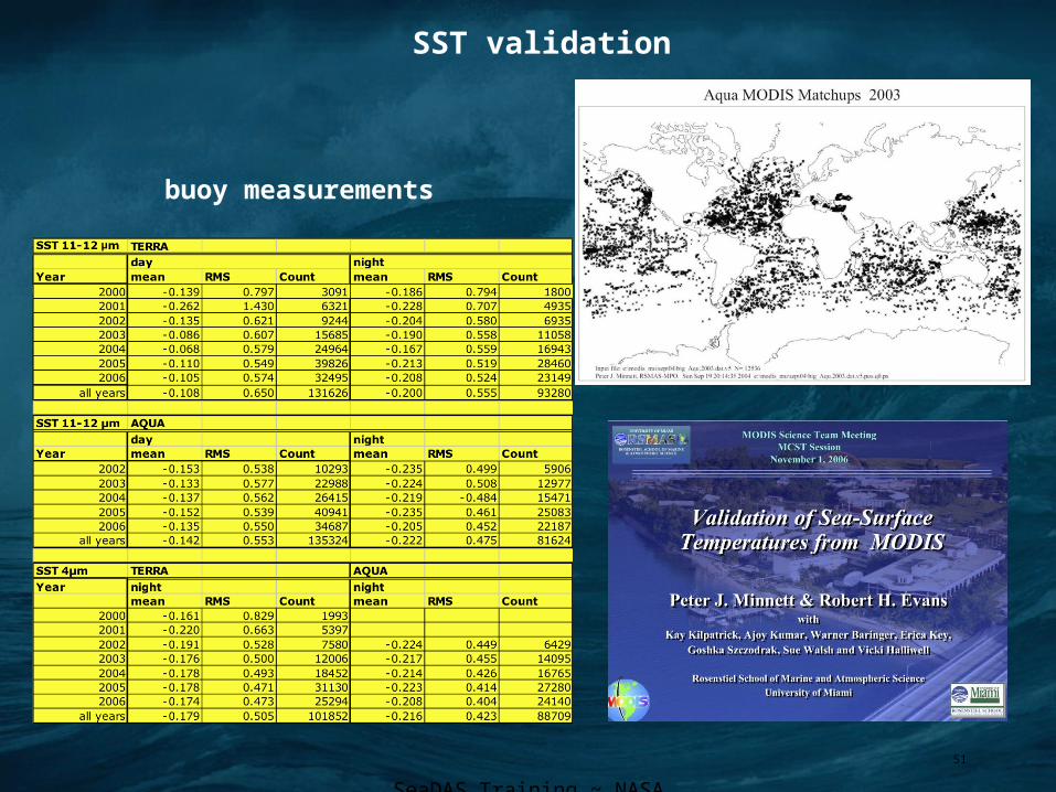
SST validation
buoy measurements

SeaDAS Training ~ NASA Ocean Biology Processing Group
52
Shortwave SST
sst4 = a0 + a1*BT39 + a2*dBT + a3*(1.0/-1.0)
where:BT39 = brightness temperature at 3.959 um, in deg-CBT40 = brightness temperature at 4.050 um, in deg-C= cosine of sensor zenith angledBT = BT39 - BT40
a0, a1, a2, a3 - fit coefficients derived derived by regression of MODIS BTs with in situ buoysvary seasonally (probably due to residual water-vapor effects)determined by science team PI (Peter Minnett and Univ. Miami staff)
SeaDAS Training ~ NASA Ocean Biology Processing Group
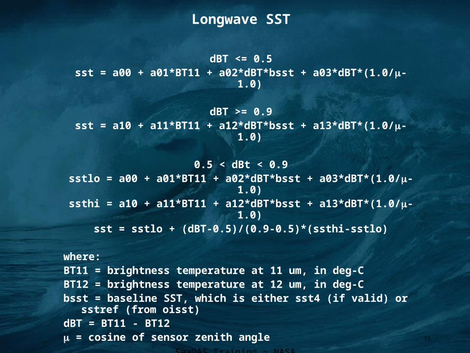
53
Longwave SST
dBT <= 0.5sst = a00 + a01*BT11 + a02*dBT*bsst + a03*dBT*(1.0/-1.0)
dBT >= 0.9sst = a10 + a11*BT11 + a12*dBT*bsst + a13*dBT*(1.0/-1.0)
0.5 < dBt < 0.9sstlo = a00 + a01*BT11 + a02*dBT*bsst + a03*dBT*(1.0/-1.0)ssthi = a10 + a11*BT11 + a12*dBT*bsst + a13*dBT*(1.0/-1.0)
sst = sstlo + (dBT-0.5)/(0.9-0.5)*(ssthi-sstlo)
where:BT11 = brightness temperature at 11 um, in deg-CBT12 = brightness temperature at 12 um, in deg-Cbsst = baseline SST, which is either sst4 (if valid) or sstref (from oisst)dBT = BT11 - BT12 = cosine of sensor zenith angle
![A Dimensions: [mm] B Recommended land pattern: [mm] · 2020. 8. 11. · 2014-03-11 2013-12-19 2013-12-04 2013-04-10 2013-03-06 2013-02-14 2012-12-10 DATE SSt SSt SSt SSt SSt SSt SSt](https://static.fdocuments.in/doc/165x107/6145e75a8f9ff812541fec6f/a-dimensions-mm-b-recommended-land-pattern-mm-2020-8-11-2014-03-11-2013-12-19.jpg)