SSRN-id2340547 hotmoneygoround

Electronic copy available at: http://ssrn.com/abstract=2340547

The Term Structure

of Currency Carry Trade Risk Premia

Hanno Lustig

UCLA and NBER

Andreas Stathopoulos

USC

Adrien Verdelhan

MIT and NBER

November 2013∗

Abstract

We find that average returns to currency carry trades decrease significantly as the ma-

turity of the foreign bonds increases, because investment currencies tend to have small local

bond term premia. The downward term structure of carry trade risk premia is informa-

tive about the temporal nature of risks that investors face in currency markets. We show

that long-maturity currency risk premia only depend on the domestic and foreign permanent

components of the pricing kernels, since transitory currency risk is automatically hedged by

interest rate risk for long-maturity bonds. Our findings imply that there is more cross-border

sharing of permanent than transitory shocks.

∗First Version: May 2013. Lustig: UCLA Anderson School of Management, 110 Westwood Plaza, SuiteC4.21, Los Angeles, CA 90095 ([email protected]). Stathopoulos: USC Marshall School of Business,3670 Trousdale Parkway, Hoffman Hall 711, Los Angeles, CA 90089 ([email protected]). Verdelhan:MIT Sloan School of Management, 100 Main Street, E62-621, Cambridge, MA 02139 ([email protected]). Manythanks to Mikhail Chernov, Ron Giammarino, Lars Hansen, Urban Jermann, Leonid Kogan, Ian Martin, TarunRamodoran, Lucio Sarno, Andrea Vedolin (discussant), Mungo Wilson, Irina Zviadadze, seminar participants atthe LSE, LBS, MIT, UC3 in Madrid, the Said School at Oxford, Cass at City University London, UBC, USC,and Wharton, as well as the participants at the First Annual Conference on Foreign Exchange Markets at theImperial College, London.


In this paper, we show that the term structure of currency carry trade risk premia is

downward-sloping: the returns to the currency carry trade are much smaller for bonds with

longer maturities. We derive a preference-free condition that links foreign and domestic long-

term bond returns, expressed in a common currency, to the permanent components of the

pricing kernels. The downward-sloping term structure of average carry trade returns is therefore

informative about the temporal nature of risks that investors face in currency markets.

Carry trades at the short end of the maturity curve are akin to selling Treasury bills in

funding currencies and buying Treasury bills in investment currencies. The exchange rate is

here the only source of risk. The set of funding and investment currencies can be determined

by the level of short-term interest rates or the slope of the yield curves, as noted by Ang and

Chen (2010). Likewise, carry trades at the long end of the maturity curve are akin to selling

long-term bonds in funding currencies and buying long-term bonds in investment currencies.

Each leg of the trade is subject to exchange rate and interest rate risk. The log return on a

foreign bond position (expressed in U.S. dollars) in excess of the domestic (i.e., U.S.) risk-free

rate is equal to the sum of the log excess bond return in local currency plus the return on a

long position in foreign currency. Therefore, average foreign bond excess returns converted in

domestic currency are the sum of a local bond term premium and a currency risk premium. The

absence of arbitrage has clear theoretical implications for those two risk premia.

On the one hand, at the short end of the maturity curve, currency risk premia are high when

there is less risk in foreign countries’ pricing kernels than at home (Bekaert, 1996; Bansal, 1997;

and Backus, Foresi, and Telmer, 2001). On the other hand, at the long end of the maturity curve,

local bond term premia compensate investors for the risk associated with temporary innovations

to the pricing kernel (Bansal and Lehmann, 1997; Alvarez and Jermann, 2005; Hansen, Heaton,

and Li, 2008; Hansen, 2009; Hansen and Scheinkman, 2009; and Bakshi and Chabi-Yo, 2012 ).

In this paper, we combine those two insights to derive three preference-free theoretical re-

sults that rely only on the absence of arbitrage in international financial markets. First, the

difference between domestic and foreign long-term bond risk premia, expressed in domestic cur-

rency terms, is pinned down by the entropies of the permanent components of the domestic and

1


foreign stochastic discount factors (SDF). This is due to the fact that the currency exposure

completely hedges the exposure of the long-short strategy in long-term bonds to the ‘unshared’

temporary pricing kernel shocks. Second, when permanent shocks are fully shared across coun-

tries and therefore exchange rates are driven by temporary innovations, bond returns in dollars

are identical across countries, date by date. We refer to this condition as the uncovered bond

return parity condition and test it in the data. Third, we derive a lower bound on the covariance

between the domestic and foreign permanent components of the pricing kernels when they are

lognormal. The lower bound depends on the difference between the maximum log return and

the return on a long-term bond in the domestic and foreign countries, as well as the volatility

of the permanent component of exchange rate changes. These three results suggest a novel look

at actual bond returns across countries.

We study the uncovered bond return parity condition both in the cross-section and in the

time-series of foreign bond returns. The theoretical results pertain to risk-free zero-coupon bonds

with infinite maturity: those characteristics are not available in practice, and thus we rely on

long-term government bonds of developed countries. Our data pertain to either long time-series

of G10 sovereign coupon bond returns over the 12/1950–12/2012 sample, or a shorter sample

(12/1971–12/2012) of G10 sovereign zero-coupon yield curves. Although we do not observe

infinite maturity bonds in either case, we find significant differences in carry trade returns

across maturities.

Between 12/1950 and 12/2012, the portfolio of flat-slope (mostly high short-term interest

rate) currencies yields a one-month currency risk premium of 3.0% and a local term premium of

−1.8% per annum (which sum to a bond premium of 1.2%). Over the same period, the portfolio

of steep-slope (mostly low short-term interest rate) currencies yields a currency risk premium

of 0.05% and a local term premium of 4.0% (which sum to a bond premium of 4.05%). The

average spread in dollar Treasury bill returns between the low slope and high slope portfolios is

thus 2.95% (3.0%− 0.05%) for Treasury bills, but it is −2.85% (1.2%− 4.05%) for the 10-year

bond portfolios. Countries with a high currency risk premium tend to have a low bond term

premium. The profitable bond strategy therefore involves shorting the carry trade currencies

2

and going long in the funding currencies. We obtain similar results when sorting countries by

the level of their short-term interest rates: the risk premia at the long end of the maturity

curve are significantly smaller that those at the short end, as the difference in local currency

bond term premia largely offsets the currency risk premium. As a result, the average returns

on foreign long-term bonds, once converted into U.S. dollars are small and rarely statistically

different from the average return on U.S. long-term bonds, as the uncovered bond return parity

condition implies on average.

The long-run uncovered bond parity condition is a better fit in the cross-section on average

than in the time series. In the post-Bretton Woods period, an 1% increase in U.S. long-term

bond returns increases foreign bond returns in dollars by an average of 0.4%. The exchange rate

exposure accounts for almost a third of this effect: the dollar appreciates on average against a

basket of foreign currencies when the U.S. bond returns are lower than average, and vice-versa,

except during flight-to-liquidity episodes. While we reject the long-run uncovered bond return

parity condition in the time series, we do find a secular increase in the sensitivity of foreign

long-term bond returns to U.S. bond returns over time, consistent with an increase in the risk-

sharing of permanent shocks in international financial markets. After 1991, an 1% increase in

U.S. long-term bond returns increases foreign bond returns in dollars by 0.5% on average. Since

bond returns expressed in dollars do not move one for one in the time-series, permanent shocks

to the foreign and domestic pricing kernels must not be perfectly shared.

To shed additional light on the nature of international risk sharing, we therefore decompose

exchange rates into their permanent and transitory components. Alvarez and Jermann (2005),

Hansen, Heaton, and Li (2008), Hansen and Scheinkman (2009), and Bakshi and Chabi-Yo

(2012) have explored the implications of such a decomposition of domestic pricing kernels for

asset prices. Given that exchange rates express differences in pricing kernels across countries,

the pricing kernel decomposition implies that exchange rate changes can be also broken into

two components, one that encodes cross-country differences in the permanent SDF components

and one that reflects differences in the transitory components. Data on long-maturity bond

returns allow us to extract the time series for two exchange rate components for a cross-section

3

of exchange rates. The characteristics of the permanent components of exchange rates are then a

key ingredient to compute our lower bound on the covariance between the domestic and foreign

permanent components of the pricing kernels.

We find that the two exchange rate components contribute about equally to the volatility of

exchange rate changes, implying that internationally unshared pricing kernel transitory shocks

are equally important to unshared permanent shocks for exchange rate determination. This

finding contrasts with previous results obtained on domestic markets. From the relative size of

the equity premium (large) and the term premium (small), Alvarez and Jermann (2005) infer

that almost all the variation in stochastic discount factors arises from permanent fluctuations.

Since permanent fluctuations are an order of magnitude larger than transitory fluctuations, our

findings imply that countries share permanent shocks to a much larger extent than transitory

fluctuations. Indeed, we show that the implied correlation of the transitory stochastic discount

factor components, although positive, is much lower than the implied correlation of state prices,

as calculated in Brandt, Cochrane, and Santa-Clara (2006). We also find that the two exchange

rate components are negatively correlated with each other: permanent innovations that raise

the state price of a given country relative to that of a foreign country tend to be partly offset

by unshared transitory innovations.

Our paper is related to three large strands of the literature: the extent of international

risk-sharing, the carry trade returns, and the term premia across countries.

The nature and magnitude of international risk sharing is a key question in macroeconomics,

and the object of a fierce debate (see, for example, Cole and Obstfeld, 1991; van Wincoop, 1994;

Lewis, 2000; Gourinchas and Jeanne, 2006; Coeurdacier, Rey, and Winant, 2013). It is well-

known since Cole and Obstfeld (1991) that the ratio of foreign and domestic marginal utilities

is tightly linked to international risk-sharing only when the domestic and foreign representative

agents consume the same baskets of goods. Under this usual assumption, the potential gains

to international risk sharing may be small for two reasons: the welfare gains from removing all

aggregate consumption uncertainty are large, but almost exclusively due to the low frequency

component in consumption, not the business cycle component (Alvarez and Jermann, 2004); the

4

bulk of the persistent shocks to the pricing kernel appear effectively traded away in international

financial markets. Our findings thus reinforce and generalize previous results in international

finance. As pointed out by Brandt, Cochrane, and Santa-Clara (2006), the combination of

relatively smooth exchange rates (10% per annum) and much more volatile stochastic discount

factors (50% per annum) implies that state prices are highly correlated across countries (at

least 0.98). Colacito and Croce (2011) argue in a long-run risk model that only the persistent

component of consumption growth is highly correlated across countries. Lewis and Liu (2012)

reach a similar conclusion. Our findings provide model-free evidence in support of the view

that the bulk of permanent shocks are shared across countries. In on-going work, Chabi-Yo

and Colacito (2013) generalize the lower bound on the comovement of domestic and foreign

permanent SDFs to pricing kernels that are not necessarily lognormal.

Our paper builds on the vast literature on uncovered interest rate parity condition (UIP) and

the currency carry trade [Engel (1996), and Lewis (2011) provide recent surveys]. We derive gen-

eral conditions under which long-run UIP follows from the absence of arbitrage: if all permanent

shocks to the pricing kernel are common, then foreign and domestic yield spreads in dollars on

long maturity bonds will be equalized, regardless of the properties of the pricing kernel. Chinn

and Meredith (2004) document some time-series evidence that supports UIP at longer holding

periods. Boudoukh, Richardson, and Whitelaw (2013) show that past forward rate differences

predict future changes in exchange rates. Lustig, Roussanov, and Verdelhan (2011) show that

asymmetric exposure to global innovations to the pricing kernel are key to understanding the

global currency carry trade premium. They identify innovations in the volatility of global equity

markets as candidate shocks, while Menkhoff, Sarno, Schmeling, and Schrimpf (2012) propose

the volatility in global currency markets instead. Building on the reduced-form model of Lustig,

Roussanov, and Verdelhan (2011), we show in closed form that if there is no heterogeneity in

the loadings of the permanent, global component of the SDF, then the foreign term premium,

once converted in U.S. dollars is the same as the U.S. term premium.

In closely related work, Koijen, Moskowitz, Pedersen, and Vrugt (2012) and Wu (2012)

examine the currency-hedged returns on ‘carry’ portfolios of international bonds, sorted by

5

a proxy for the carry on long-term bonds, but they do not examine the interaction between

currency and term risk premia, the topic of our paper. We focus on portfolios sorted by interest

rates, as well as yield spreads, since it is well-know since Campbell and Shiller (1991) that yield

spreads can predict excess returns on bonds. As already noted, Ang and Chen (2010) were the

first to show that yield curve variables can also be used to forecast currency excess returns, but

these authors do not examine the returns on foreign bond portfolios. Dahlquist and Hasseltoft

(2013) study international bond risk premia in an affine asset pricing model and find evidence

for local and global risk factors. Jotikasthira, Le, and Lundblad (2012) report similar findings.

Our paper revisits the empirical evidence on bond returns without committing to a specific term

structure model.

The rest of the paper is organized as follows. In Section 1, we derive the no-arbitrage,

preference-free theoretical restrictions imposed on currency and term risk premia. In Section

2, we provide three simple theoretical examples. In Section 3, we examine the cross-section of

bond excess returns in local currency and in U.S. dollars and contrasts it to the cross-section

of currency excess returns. In Section 4, we test the uncovered bond return parity condition

in the time-series. In Section 5, we decompose exchange rate changes into a permanent and

a temporary component and links their properties to the extent of risk-sharing. In Section 6,

we present concluding remarks. The Online Appendix contains all proofs and supplementary

material not presented in the main body of the paper.

1 The Term Premium and the Currency Risk Premium

We begin by defining notation and then deriving our main theoretical results.

1.1 Notation

In order to state our main results, we first need to introduce the domestic and foreign pricing

kernels, SDFs, and bond holding period returns.

6

Pricing Kernel, Stochastic Discount Factor, and Bond Return The nominal pricing

kernel is denoted Λt($); it corresponds to the marginal value of a dollar delivered at time

t in some state of the world $. The nominal SDF is the growth rate of the pricing kernel:

Mt+1 = Λt+1/Λt. The price of a zero-coupon bond that matures k periods into the future is

given by:

P(k)t = Et

(Λt+kΛt

).

The one-period return on the zero-coupon bond with maturity k is R(k)t+1 = P

(k−1)t+1 /P

(k)t . The

log excess returns, denoted rx(k)t+1, is equal to logR

(k)t+1/R

ft , where the risk-free rate are Rft =

R(0)t+1 = 1/P

(1)t . The expected log excess return on the zero-coupon bond with maturity k, or

term premium, is:

Et

[rx

(k)t+1

]= Et

[logR

(k)t+1/R

ft

].

The yield spread is the log difference between the yield of the k-period bond and the risk-free

rate: y(k)t = log

(Rft /(P

(k)t )1/k

).

Entropy Bond returns and SDFs are volatile, but not necessarily normally distributed. In

order to measure the time-variation in their volatility, it is convenient to use entropy.1 The

conditional volatility of any random variable Xt+1 is thus measured through its conditional

entropy Lt, defined as:

Lt (Xt+1) = logEt (Xt+1)− Et (logXt+1) .

The conditional entropy of a random variable is determined by its conditional variance, as well

as its higher moments; if vart (Xt+1) = 0, then Lt (Xt+1) = 0, but the reverse is not generally

true. If Xt+1 is conditionally lognormal, then the entropy is simply the half variance of the log

variable: Lt (Xt+1) = (1/2)vart (logXt+1). The relative entropy of the permanent and transitory

components of the domestic and foreign SDFs turns out to be key to understanding the term

structure of carry trade risk.

1Backus, Chernov, and Zin (2012) make a convincing case for the use of entropy in assessing macro-financemodels.

7

Permanent and Transitory Innovations Following Alvarez and Jermann (2005), Hansen,

Heaton, and Li (2008), and Hansen and Scheinkman (2009), we decompose each pricing kernel

into a transitory (ΛTt ) component and a permanent (ΛP

t ) component with:

Λt = ΛPt ΛT

t , where ΛTt = lim

k→∞

δt+k

P(k)t

.

The constant δ is chosen to satisfy the following regularity condition: 0 < limk→∞

P(k)t

δk<∞ for all

t. We also assume that, for each t+ 1, there exists a random variable xt+1 with finite Et(xt+1)

such that a.s. Λt+1

δt+1

P(k)t+1

δk≤ xt+1 for all k. Under those regularity conditions, the infinite maturity

bond return is then:

R(∞)t+1 = lim

k→∞R

(k)t+1 = lim

k→∞P

(k−1)t+1 /P

(k)t =

ΛTt

ΛTt+1

.

The permanent component, ΛPt , is a martingale.2 It is an important component of the pricing

kernel. Alvarez and Jermann (2005) derive a lower bound on its volatility, and, given the size of

the equity premium relative to the term premium, conclude that the permanent component of

the pricing kernel is large and accounts for most of the risk.3 In other words, a lot of persistence

is needed to deliver a low term premium and a high equity premium. In the absence of arbitrage,

Alvarez and Jermann (2005) show that the local term premium in local currency is given by:

Et

[rx

(∞)t+1

]= lim

k→∞Et

[rx

(k)t+1

]= Lt

(Λt+1

Λt

)− Lt

(ΛPt+1

ΛPt

).

Hansen, Heaton, and Li (2008), Hansen and Scheinkman (2009), and Borovicka, Hansen,

Hendricks, and Scheinkman (2011) provide examples of similar factorizations in affine models.

The SDF decomposition defined here is subject to important limitations that need to be high-

2Note that ΛPt is equal to:

ΛPt = lim

k→∞

P(k)t

δt+kΛt = lim

k→∞

Et(Λt+k)

δt+k.

The second regularity condition ensures that the expression above is a martingale.3Alvarez and Jermann (2005) derive the following lower bound:

Lt

(ΛP

t+1

ΛPt

)≥ Et (logRt+1)− Et

(logR

(∞)t+1

),

where Rt+1 denotes any positive return and R(∞)t+1 is the return on a zero-coupon bond of infinite maturity.

8

lighted. Hansen and Scheinkman (2009) point out that this decomposition is not unique in

general and provide parametric examples in which uniqueness fails. In addition, the temporary

(or transient) and permanent components are potentially highly correlated, which complicates

their interpretation.4 Despite these limitations, we show that this decomposition proves to be

particularly useful when analyzing foreign bond returns at longer maturities.

Exchange Rates The spot exchange rate in foreign currency per U.S. dollar is denoted St.

When S increases, the U.S. dollar appreciates. Similarly, Ft denotes the one-period forward

exchange rate, and ft its log value. When markets are complete, the change in the exchange

rate corresponds to the ratio of the domestic to foreign SDFs:

St+1

St=

Λt+1

Λt

Λ∗tΛ∗t+1

,

where ∗ denotes a foreign variable. The no-arbitrage definition of the exchange rate comes

directly from the Euler equations of the domestic and foreign investors, for any asset R expressed

in foreign currency: Et[Mt+1R∗t+1St/St+1] = 1 and Et[M

∗t+1R

∗t+1] = 1. When markets are

complete, the SDF is unique, and thus the change in exchange rate is the ratio of the two SDFs.

The exchange rate is not constant as soon as good markets are not frictionless. The log currency

excess return corresponds to:

rxFXt+1 = log

[StSt+1

Rf,∗t

Rft

]= (ft − st)−∆st+1,

when the investor borrows at the domestic risk-free rate, Rft , and invests at the foreign risk-

free rate, Rf,∗t , and where the forward rate is defined through the covered interest rate parity

condition: Ft/St = Rf,∗t /Rft . As Bekaert (1996) and Bansal (1997) show, in a lognormal model,

the log currency risk premium equals the half difference between the conditional volatilities

of the log domestic and foreign SDFs. Gavazzoni, Sambalaibat, and Telmer (2012), however,

4The authors thank Lars Hansen for a detailed account of these issues.

9

convincingly argue that higher moments are critical for understanding currency returns.5 When

higher moments matter and markets are complete, the currency risk premium is equal to the

difference between the entropy of the domestic and foreign SDFs (Backus, Foresi, and Telmer,

2001):

Et[rxFXt+1

]= (ft − st)− Et(∆st+1) = Lt

(Λt+1

Λt

)− Lt

(Λ∗t+1

Λ∗t

).

Following the decomposition of the pricing kernel discussed above, exchange rate changes

can also be decomposed into a permanent and a transitory component, defined below:

St+1

St=

(ΛPt+1

ΛPt

ΛP,∗t

ΛP,∗t+1

)(ΛTt+1

ΛTt

ΛT,∗t

ΛT,∗t+1

)=SPt+1

SPt

STt+1

STt

.

Exchange rate changes capture the differences in both the transitory and the permanent compo-

nent of the two countries’ SDFs. In this paper, we use returns on long term bonds to implement

this decomposition in the data.

Term Premium on Foreign Bonds The log return on a foreign bond position (expressed

in U.S. dollars) in excess of the domestic (i.e., U.S.) risk-free rate is denoted rx(k),$t+1 . It can be

expressed as the sum of the log excess return in local currency plus the return on a long position

in foreign currency:

rx(k),$t+1 = log

[R

(k),∗t+1

Rft

StSt+1

]= log

[R

(k),∗t+1

Rf,∗t

Rf,∗t

Rft

StSt+1

]= rx

(k),∗t+1 + rxFXt+1.

The first component of the foreign bond excess return is the excess return on a bond in foreign

currency, while the second component represents the log excess return on a long position in

foreign currency, given by the forward discount minus the rate of depreciation. Taking expecta-

tions, the total term premium in dollars thus consists of a foreign bond risk premium, Et[rx(k),∗t+1 ],

plus a currency risk premium, (ft − st)− Et∆st+1.

5In earlier work, Brunnermeier, Nagel, and Pedersen (2009) show that risk reversals increase with interestrates. Jurek (2008) provides a comprehensive empirical investigation of hedged carry trade strategies. Gourio,Siemer, and Verdelhan (2013) study a real business cycle with disaster risk. Farhi, Fraiberger, Gabaix, Ranciere,and Verdelhan (2013) estimate a no-arbitrage model with crash risk using a cross-section of currency options.Chernov, Graveline, and Zviadadze (2011) study jump risk at high frequencies.

10

1.2 Main Theoretical Results

In this section, we present our four key theoretical results on (i) the term structure of carry trade

premia; (ii) the decomposition of exchange rates into permanent and transitory components;

(iii) the long-term bond return parity condition; and (iv) a lower bound on the risk-sharing of

permanent shocks.

Carry Trade Term Premia We begin with a characterization of carry trade risk premia at

long maturities.

Proposition 1. The foreign term premium in dollars is equal to the domestic term premium

plus the difference between the domestic and foreign entropies of the permanent components of

the pricing kernels:

Et

[rx

(∞),∗t+1

]+ (ft − st)− Et[∆st+1] = Et

[rx

(∞)t+1

]+ Lt

(ΛPt+1

ΛPt

)− Lt

(ΛP,∗t+1

ΛP,∗t

).

In order to deliver a currency risk premium at longer maturities, entropy differences in

the permanent component of the pricing kernel are required. If there are no such differences

and domestic and foreign pricing kernels are symmetric, then high local currency term premia

coincide with low currency risk premia and vice-versa. In the symmetric case, dollar term premia

are identical across currencies. At shorter maturities, the currency risk premium is determined

by the entropy difference of the entire pricing kernel. Since carry trade returns are base-currency-

invariant, heterogeneity in the exposure of the pricing kernel to a global component of the pricing

kernel is required to explain the carry trade premium (Lustig, Roussanov, and Verdelhan, 2011).

Clearly, a carry trade premium at longer maturities exists only with heterogeneous exposure to

a permanent global component.

Permanent Component of Exchange Rates The valuation of long-maturity bonds thus

encodes information about the nature of shocks that drive the changes in exchange rates. Using

11

the prices of long-maturity bonds in the domestic and foreign countries, under the regularity

conditions defined previously, we can decompose the changes in the bilateral spot exchange rate

into two parts: a part that captures cross-country differences in the transitory components of the

pricing kernel and a part that encodes differences in the permanent components of the pricing

kernel.

Proposition 2. When markets are complete, the ratio of the domestic and foreign infinite

maturity bond returns, expressed in the same currency, measures the permanent component of

exchange rate changes:

limk→∞

StSt+1

R(k),∗t+1

R(k)t+1

=ΛP,∗t+1

ΛP,∗t

ΛPt

ΛPt+1

=SPt

SPt+1

.

The left-hand side of this equality can be approximated by long term bonds, thus leading to

a measure of the permanent component of exchange rates. Since exchange rates are observed,

the temporary component of the exchange rates can also be easily obtained.

Long-Term Bond Return Parity Condition The exchange rate decomposition above im-

plies an uncovered long-bond return parity condition when countries share permanent innova-

tions to their SDFs. In this polar case, even if most of the innovations to the pricing kernel are

highly persistent, the shocks that drive exchange rates are not, because the persistent shocks

are shared across countries.

Corollary 1. If the domestic and foreign pricing kernels have common permanent innovations,

ΛPt+1/Λ

Pt = ΛP,∗

t+1/ΛP,∗t for all states, then the one-period returns on the foreign longest maturity

bonds in domestic currency are identical to the domestic ones: R(∞),∗t+1

StSt+1

= R(∞)t+1 for all states.

Risk-Sharing The exchange rate decomposition also sheds light on cross-country risk-sharing.

Brandt, Cochrane, and Santa-Clara (2006) show that the combination of relatively smooth

exchange rates and much more volatile SDFs implies that state prices are very highly correlated

across countries. A 10% volatility in exchange rate changes and a volatility of marginal utility

12

growth rates of 50% imply a correlation of at least 0.98. We can derive a specific bound on the

covariance of the permanent component across different countries.

Proposition 3. If the permanent SDF component is unconditionally lognormal, the cross-

country covariance of the SDF’ permanent components is bounded below by:

cov

(log

ΛP,∗t+1

ΛP,∗t

, logΛPt+1

ΛPt

)≥ E

(log

R∗t+1

R(∞),∗t+1

)+ E

(log

Rt+1

R(∞)t+1

)− 1

2var

(log

SPt+1

SPt

).

for any positive returns Rt+1 and R∗t+1. A conditional version of the expression holds for con-

ditionally lognormal permanent pricing kernel components.

We can compute the variance of the permanent component of exchange rates, var(

logSPt+1

SPt

),

in the data; the contribution of the last term will typically be on the order of 1% or less — this

value will be discussed in our empirical work. Given the large size of the equity premium

compared to the term premium (a 7.5% difference according to Alvarez and Jermann, 2005),

and the relatively small variance of the permanent component of exchange rates, this bound

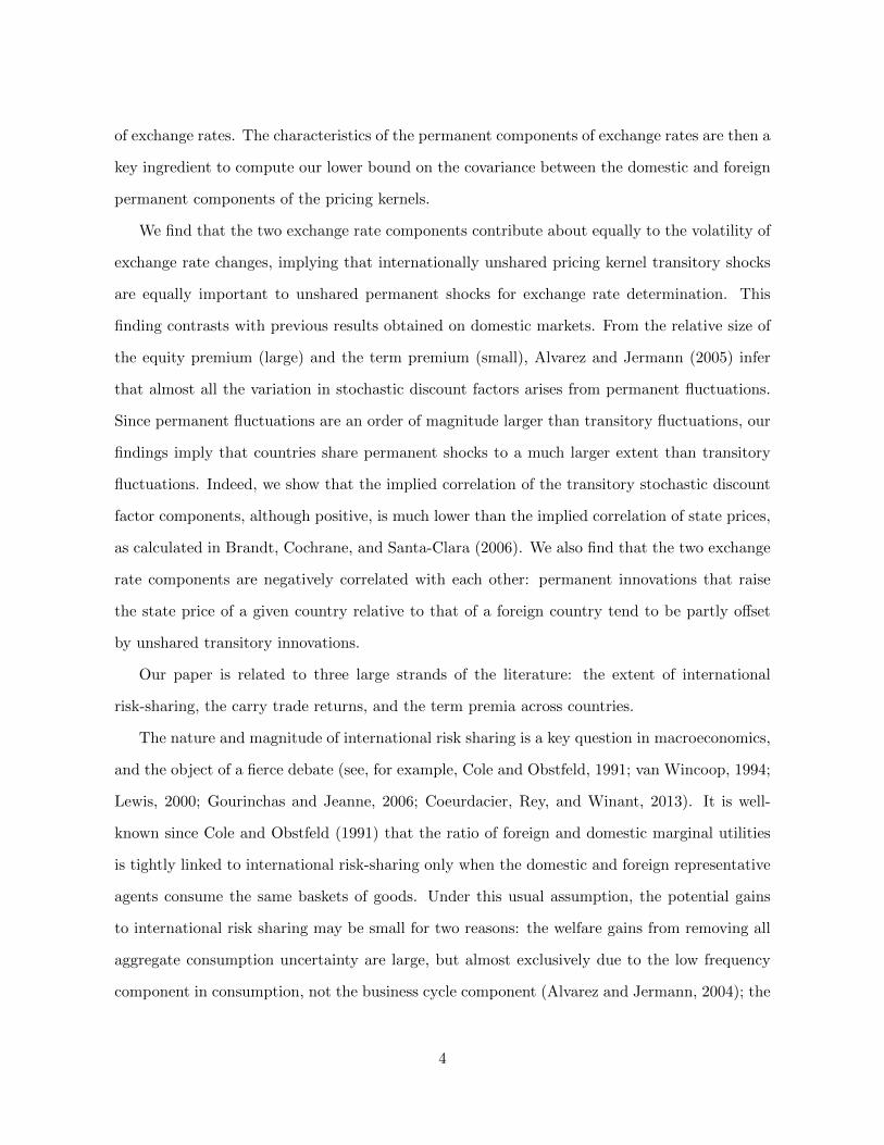
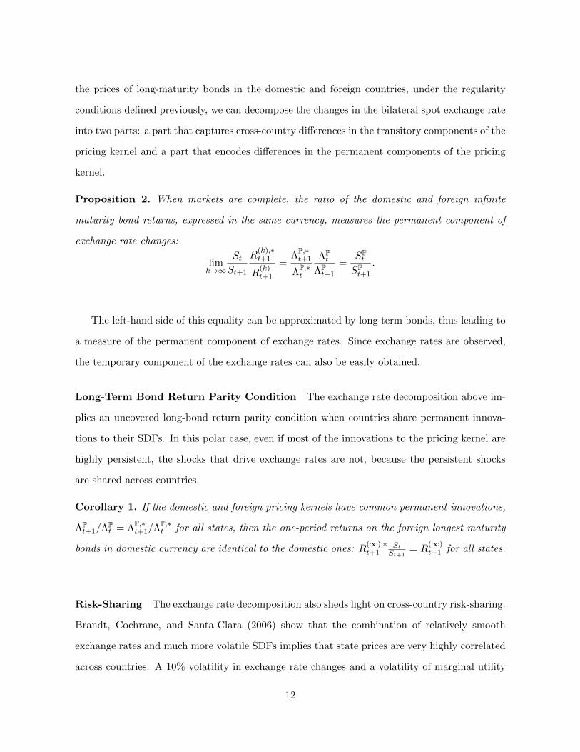
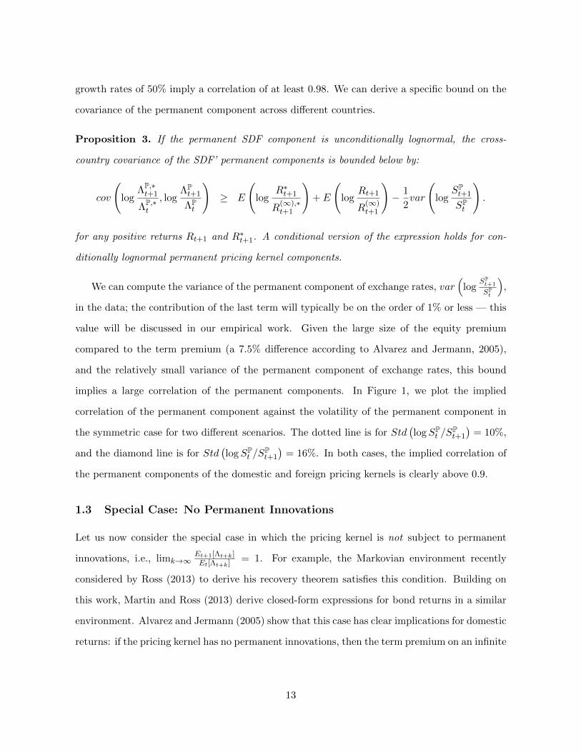
implies a large correlation of the permanent components. In Figure 1, we plot the implied

correlation of the permanent component against the volatility of the permanent component in

the symmetric case for two different scenarios. The dotted line is for Std(logSP

t /SPt+1

)= 10%,

and the diamond line is for Std(logSP

t /SPt+1

)= 16%. In both cases, the implied correlation of

the permanent components of the domestic and foreign pricing kernels is clearly above 0.9.

1.3 Special Case: No Permanent Innovations

Let us now consider the special case in which the pricing kernel is not subject to permanent

innovations, i.e., limk→∞Et+1[Λt+k]Et[Λt+k] = 1. For example, the Markovian environment recently

considered by Ross (2013) to derive his recovery theorem satisfies this condition. Building on

this work, Martin and Ross (2013) derive closed-form expressions for bond returns in a similar

environment. Alvarez and Jermann (2005) show that this case has clear implications for domestic

returns: if the pricing kernel has no permanent innovations, then the term premium on an infinite

13

0.4 0.5 0.6 0.7 0.8 0.9 10

0.1

0.2

0.3

0.4

0.5

0.6

0.7

0.8

0.9

1

Volatility of Permanent Component

Implie

d C

orr

ela

tion

10%

16%

Figure 1: Permanent Risk Sharing — In this figure, we plot the implied correlation of the domestic andforeign permanent components of the SDF against the standard deviation of the permanent component of theSDF. The dotted line is for Std

(logSP

t /SPt+1

)= 10%. The straight line is for Std

(logSP

t /SPt+1

)= 16%. Following

Alvarez and Jermann (2005), we assume that the domestic and foreign equity minus bond risk premia are 7.5%.

maturity bond is the largest risk premium in the economy.6

This case also has a strong implication for the term structure of the carry trade risk premia.

When the pricing kernels do not have permanent innovations, the foreign term premium in

dollars equals the domestic term premium:

Et

[rx

(∞),∗t+1

]+ (ft − st)− Et[∆st+1] = Et

[rx

(∞)t+1

].

The proof here is straightforward. In general, the foreign currency risk premium is equal to

6 If there are no permanent innovations to the pricing kernel, then the return on the bond with the longestmaturity equals the inverse of the SDF: limk→∞R

(k)t+1 = Λt/Λt+1. High marginal utility growth translates into

higher yields on long maturity bonds and low long bond returns, and vice-versa.

14

the difference in entropy. In the absence of permanent innovations, the term premium is equal

to the entropy of the pricing kernel, so the result follows. More interestingly, a much stronger

result holds in this case. Not only are the risk premia identical, but the returns on the foreign

bond position are the same as those on the domestic bond position state-by-state, because the

foreign bond position automatically hedges the currency risk exposure. As already noted, if the

domestic and foreign pricing kernels have no permanent innovations, then the one-period returns

on the longest maturity foreign bonds in domestic currency are identical to the domestic ones:

limk→∞

StSt+1

R(k),∗t+1

R(k)t+1

= 1.

In this class of economies, the returns on long-term bonds expressed in domestic currency are

equalized:

limk→∞

rx(k),∗t+1 + (ft − st)−∆st+1 = rx

(k)t+1.

In countries that experience higher marginal utility growth, the domestic currency appreciates

but is exactly offset by the capital loss on the bond. For example, in a representative agent

economy, when the log of aggregate consumption drops more below trend at home than abroad,

the domestic currency appreciates, but the real interest rate increases, because the representative

agent is eager to smooth consumption. The foreign bond position automatically hedges the

currency exposure.

2 Three Theoretical Lognormal Examples

This section provides three lognormal examples of the theoretical results derived above. We start

with a simple homoscedastic SDF suggested by Alvarez and Jermann (2005), and then turn to

a heteroscedastic SDF like the one proposed by Cox, Ingersoll, and Ross (1985). Building on

these two preliminary examples and on Lustig, Roussanov, and Verdelhan (2011), the section

ends with a model featuring global permanent and transitory shocks. This model illustrates the

necessary conditions for the cross-sections of carry and term premia.

15

2.1 Homoscedastic SDF

Alvarez and Jermann (2005) propose the following example of an economy without permanent

shocks: a representative agent economy with power utility investors in which the log of aggregate

consumption is a trend-stationary process with normal innovations:

log Λt =

∞∑i=0

αiεt−i + β log t,

with ε ∼ N(0, σ2), α0 = 1. If limk→∞ α2k = 0, then the SDF has no permanent component. The

foreign SDF is defined similarly. In this example, Alvarez and Jermann (2005) show that the

term premium equals one half of the variance: Et

[rx

(∞)t+1

]= σ2/2. In this case, we find that the

foreign term premium in dollars is identical to the domestic term premium:

Et

[rx

(∞),∗t+1

]+ (ft − st)− Et[∆st+1] =

1

2σ2 = Et

[rx

(∞)t+1

].

This result is straightforward to establish: recall that the currency risk premium is equal to

the half difference in the domestic and foreign SDF volatilities. Currencies with a high local

currency term premium (high σ2) also have an offsetting negative currency risk premium, while

those with a small term premium have a large currency risk premium. Hence, U.S. investors

receive the same dollar premium on foreign as on domestic bonds. There is no point in chasing

high term premia around the world, at least not in economies with only temporary innovations

to the pricing kernel. Currencies with the highest local term premia also have the lowest (i.e.,

most negative) currency risk premia.

Building on the previous example, Alvarez and Jermann (2005) consider a log-normal model

of the pricing kernel that features both permanent and transitory shocks:

log ΛPt+1 = −1

2σ2P + log ΛP

t + εPt+1,

log ΛTt+1 = log βt+1 +

∞∑i=0

αiεTt+1−i,

16

where α is a square summable sequence, and εP and εT are i.i.d. normal variables with mean

zero and covariance σTP . A similar decomposition applies to the foreign SDF. In this case,

Alvarez and Jermann (2005) show that the term premium is given by the following expression:

Et

[rx

(∞)t+1

]= σ2

T /2 + σTP . In this economy, the foreign term premium in dollars is:

Et

[rx

(∞),∗t+1

]+ (ft − st)− Et[∆st+1] =

1

2

(σ2 − σ2,∗

P

).

Provided that σ2,∗P = σ2

P , the foreign term premium in dollars equals the domestic term premium:

Et

[rx

(∞),∗t+1

]+ (ft − st)− Et[∆st+1] =

1

2σ2T + σTP = Et

[rx

(∞)t+1

].

2.2 Heteroscedastic SDFs: Cox, Ingersoll, and Ross (1985)

We turn now to a workhorse model in the term structure literature: the Cox, Ingersoll, and Ross

(1985) model (denoted CIR). The SDF M is defined by the following two equations:

− logMt+1 = α+ χzt +√γztut+1,

zt+1 = (1− φ)θ + φzt − σ√ztut+1.

In this model, log bond prices are affine in the state variable z: p(n)t = −Bn

0 − Bn1 zt, where Bn

0

and Bn1 are the solution to difference equations. The expected log excess return of an infinite

maturity bond is then:

Et

[rx

(∞)t+1

]=

[−1

2(B∞1 )2 σ2 + σ

√γB∞1

]zt =

[B∞1 (1− φ)− χ+

1

2γ

]zt,

where B∞1 is defined implicitly in the following second-order equation: B∞1 = χ− γ/2 +B∞1 φ−

(B∞1 )2 σ2/2+σ√γB∞1 . The first component, − (B∞1 )2 σ2/2, is a Jensen term. The term premium

is driven by the second component, σ√γB∞1 zt. In the CIR model, there are no permanent

innovations to the pricing kernel provided that B∞1 (1 − φ) = χ. In this case, the permanent

17

component of the pricing kernel is constant:

ΛPt+1

ΛPt

= β−1e−α−χθ.

In the case of no permanent innovations in the CIR model, the expected long-run term premium

is simply Et

[rx

(∞)t+1

]= γzt/2. Hence, in the symmetric case, the foreign term premium in dollars

is equal to the domestic term premium:

Et

[rx

(∞),∗t+1

]+ (ft − st)− Et[∆st+1] =

1

2γzt = Et

[rx

(∞)t+1

].

This result is equivalent to uncovered interest rate parity for very long holding periods. The

proof relies on an insight from Alvarez and Jermann (2005). They show that when the limits

of the k-period bond risk premium and the yield difference between the k-period discount bond

and the one-period riskless bond (when the maturity k tends to infinity) are well defined and

the unconditional expectations of holding returns are independent of calendar time, then the

average term premium equals the average yield difference. In the CIR model without permanent

shocks, the average foreign yield spread in dollars is identical to the domestic yield spread, an

example of a long-run uncovered interest rate parity condition:

y(∞),∗t + (ft − st)− E[ lim

k→∞

1

k

k∑j=1

∆st+j ] =1

2σ2 = y

(∞)t .

2.3 Heteroscedastic SDFs: Lustig, Roussanov, and Verdelhan (2011)

Lustig, Roussanov, and Verdelhan (2011) show that the CIR model with (i) global shocks and (ii)

heterogeneity in the SDFs’ loadings on those global shocks can replicate the empirical evidence

on currency excess returns.7 Building on their work, we turn now to a version of the CIR model

with two global components: a persistent component and a transitory component. We show

that heterogeneity in the SDFs’ loadings on the permanent global shocks is key to obtaining

7The model parameters must satisfy the two following constraints: interest rates must be pro-cyclical withrespect to the state variables, and high interest rate countries must load less on the global shocks than low interestrate countries.

18

a cross-section of foreign term premia expressed in U.S. dollars. The model is defined by the

following set of equations:

− logMt+1 = α+ χzt +√γztut+1 + τzPt +

√δzPt u

Pt+1,

zt+1 = (1− φ)θ + φzt − σ√ztut+1,

zPt+1 = (1− φP)θP + φPzPt − σP√zPt u

Pt+1,

where zt is the transitory factor, and zPt is the permanent factor. Note that the model abstracts

from the country-specific shocks and state variables; they can be added easily as in Lustig,

Roussanov, and Verdelhan (2011).

The nominal log zero-coupon n-month yield of maturity in local currency is given by the

standard affine expression y(n)t = − 1

n

(An +Bnzt + Cnz

Pt

), where the coefficients satisfy second-

order difference equations. The nominal log risk-free interest rate is an affine function of the

persistent and transitory factors: rft = α+(χ− 1

2γ)zt+

(τ − 1

2δ)zpt . In this model, the expected

log excess return on an infinite maturity bond is:

Et[rx(∞)t+1 ] =

[B∞(1− φ)− χ+

1

2γ

]zt −

[C∞(1− φp) + τ − 1

2δ

]zPt .

To give content to the notion that zt is transitory, we impose that B∞(1 − φ) = χ. This

restriction implies that the permanent component of the pricing kernel is not affected by the

transitory factor zt, as can easily be verified. In this case, the permanent component of the SDF

reduces to:

MPt+1

MPt

=Mt+1

Mt

(MTt+1

MTt

)−1

= β−1e−α−χθe−C∞

[(φP−1)(zPt−θP)−σP

√zPt ut+1

],

which does not depend on zt. Given this restriction, the bond risk premium is equal to:

Et[rx(∞)t+1 ] =

1

2γzt −

[τ − 1

2δ + C∞(1− φP)

]zPt .

Both factors are common across countries, but, following Lustig, Roussanov, and Verdelhan

19

(2011), we allow for heterogeneous loadings on these common factors. The foreign SDF is

therefore defined as:

− logM∗t+1 = α+ χzt +√γ∗ztut+1 + τzPt +

√δ∗zPt u

Pt+1.

The log currency risk premium is equal to: Et[rxFXt+1] = (γ−γ∗)zt/2 + (δ− δ∗)zPt /2. This implies

that the expected foreign log holding period return on a foreign long bond converted into U.S.

dollars is equal to:8

Et[rx(∞),$t+1 ] = Et[rx

(∞),∗t+1 ] + Et[rx

FXt+1] =

1

2γzt −

[τ − 1

2δ + C∞,∗(1− φP)

]zPt .

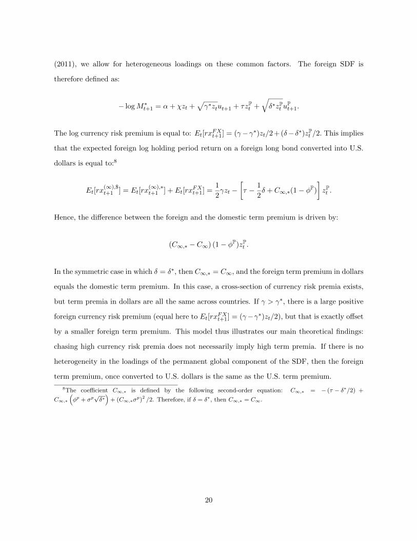
Hence, the difference between the foreign and the domestic term premium is driven by:

(C∞,∗ − C∞) (1− φP)zPt .

In the symmetric case in which δ = δ∗, then C∞,∗ = C∞, and the foreign term premium in dollars

equals the domestic term premium. In this case, a cross-section of currency risk premia exists,

but term premia in dollars are all the same across countries. If γ > γ∗, there is a large positive

foreign currency risk premium (equal here to Et[rxFXt+1] = (γ−γ∗)zt/2), but that is exactly offset

by a smaller foreign term premium. This model thus illustrates our main theoretical findings:

chasing high currency risk premia does not necessarily imply high term premia. If there is no

heterogeneity in the loadings of the permanent global component of the SDF, then the foreign

term premium, once converted to U.S. dollars is the same as the U.S. term premium.

8The coefficient C∞,∗ is defined by the following second-order equation: C∞,∗ = − (τ − δ∗/2) +

C∞,∗

(φp + σp

√δ∗)

+ (C∞,∗σp)2 /2. Therefore, if δ = δ∗, then C∞,∗ = C∞.

20

3 The Cross-Section of Long-Term Bond Returns

The empirical experiment is defined by the main theoretical results presented in Section 1. For

the reader’s convenience, we summarize them here in three equations:

Et[rxFXt+1

]= (ft − st)− Et(∆st+1) = Lt

(Λt+1

Λt

)− Lt

(Λ∗t+1

Λ∗t

)(1)

Et

[rx

(∞),∗t+1

]= lim

k→∞Et

[rx

(k),∗t+1

]= Lt

(Λ∗t+1

Λ∗t

)− Lt

(Λ∗,Pt+1

Λ∗,Pt

)(2)

Et

[rx

(∞),∗t+1

]+ Et

[rxFXt+1

]= Et

[rx

(∞)t+1

]+ Lt

(ΛPt+1

ΛPt

)− Lt

(ΛP,∗t+1

ΛP,∗t

). (3)

Equation (1) shows that the currency risk premium is equal to the difference between the entropy

of the domestic and foreign SDFs (Backus, Foresi, and Telmer, 2001). Equation (2) shows that

the term premium is equal to the difference between the total entropy of the SDF and the

entropy of its permanent component (Alvarez and Jermann, 2005). Equation (3) shows that the

foreign term premium in dollars is equal to the domestic term premium plus the difference in

the entropy of the permanent component of the pricing kernel of the domestic and the foreign

country. Our empirical work thus focuses on three average excess returns: the currency risk

premium, the term premium in foreign currency, and the term premium in U.S. dollars. To test

the predictions of the theory, we sort currencies into portfolios based on variables that can be

used to predict bond and currency returns: the slope of the yield curve and then the level of

short-term interest rates. Returns are computed over horizons of one, three, and twelve months.

In all cases, portfolios formed at date t only use information available at that date. Portfolios

are rebalanced monthly.

3.1 Samples

The benchmark sample consists of a small homogeneous panel of developed countries with rea-

sonably liquid bond markets. This G-10 panel includes Australia, Canada, Japan, Germany,

Norway, New Zealand, Sweden, Switzerland, and the U.K. The domestic country is the United

States. It only includes one country from the eurozone, Germany. For robustness checks, we

21

consider two additional sets of countries: first, a larger sample of 20 developed countries (Aus-

tralia, Austria, Belgium, Canada, Denmark, Finland, France, Germany, Greece, Ireland, Italy,

Japan, the Netherlands, New Zealand, Norway, Portugal, Spain, Sweden, Switzerland, and the

U.K.), and second, a large sample of 30 developed and emerging countries (Australia, Austria,

Belgium, Canada, Denmark, Finland, France, Germany, Greece, India, Ireland, Italy, Japan,

Mexico, Malaysia, the Netherlands, New Zealand, Norway, Pakistan, the Philippines, Poland,

Portugal, South Africa, Singapore, Spain, Sweden, Switzerland, Taiwan, Thailand, and the

U.K.).

In order to build the longest time-series possible, we obtain data from Global Financial

Data. The dataset includes a 10-year government bond total return index for each of our target

countries in dollars and in local currency and a Treasury bill total return index. The 10-year

bond returns are a proxy for the bonds with the longest maturity. Log returns on the currency

carry trade (rxFX) and the log returns on the bond portfolio in local currency (rx(10),∗) and

in U.S. dollars (rx(10),$) are first obtained at the country level. Then, portfolio returns are

obtained by averaging these log returns across all countries in a portfolio. The benchmark

sample is summarized by three portfolios while the other two samples are summarized by four

and five portfolios. For each set of countries, we report averages over the 12/1950–12/2012 and

12/1971–12/2012 periods. The main text focuses on the benchmark sample, while the Online

Appendix reports detailed results for the robustness checks.

While Global Financial Data offers, to the best of our knowledge, the longest time-series

of government bond returns available, the series have three key limits. First, they pertain to

discount bonds, while the theory pertains to zero-coupon bonds. Second, they include default

risk, while the theory focuses on default-free bonds. Third, they only offer 10-year bond returns,

not the entire term structure of bond returns. To address these issues, we use zero-coupon

bonds obtained from the estimation of term structure curves using government notes and bonds

and interest rate swaps of different maturities; the time-series are shorter and dependent on

the term structure estimations. In contrast, bond return indices, while spanning much longer

time-periods, offer model-free estimates of bond returns. Our results turn out to be similar in

22

both samples.

Our zero-coupon bond dataset consists of a panel of the benchmark sample of countries from

12/1971 to 12/2012. To construct our sample, we use the entirety of the dataset in Wright (2011)

and complement the sample, as needed, with sovereign zero-coupon curve data sourced from

Bloomberg. The panel is unbalanced: for each currency, the sample starts with the beginning

of the Wright (2011) dataset.9 Yields are available at maturities from 3 months to 15 years, in

3-month increments. We also construct an extended version of this dataset which, in addition

to the countries of the benchmark sample, includes the following countries: Austria, Belgium,

the Czech Republic, Denmark, Finland, France, Hungary, Indonesia, Ireland, Italy, Malaysia,

Mexico, the Netherlands, Poland, Portugal, Singapore, South Africa, and Spain. The data for

the aforementioned extra countries are sourced from Bloomberg.10

3.2 Sorting Currencies by the Slope of the Yield Curve

Let us start with portfolios of countries sorted by the slope of their yield curve. Recall that the

slope of the yield curve, a measure of the term premium, is largely determined by the entropy

of the temporary component of the pricing kernel. As this entropy increases, the local term

premium increases as well. However, the dollar term premium only compensates investors for the

relative entropy of the permanent component of the U.S. and the foreign pricing kernel, because

the interest rate risk associated with the temporary innovations is hedged by the currency risk.

In the extreme case in which all permanent shocks are common, the dollar term premium should

equal the U.S. term premium.

Benchmark Sample Figure 2 presents the composition over time of portfolios of the 9 cur-

rencies of the benchmark sample sorted by the slope of the yield curve. There is substantial

9The starting dates for each country are as follows: 2/1987 for Australia, 1/1986 for Canada, 1/1973 for Ger-many, 1/1985 for Japan, 1/1990 for New Zealand, 1/1998 for Norway, 12/1992 for Sweden, 1/1988 for Switzerland,1/1979 for the U.K., and 12/1971 for the U.S. For New Zealand, the data for maturities above 10 years start in12/1994.

10The starting dates for the additional countries are as follows: 12/1994 for Austria, Belgium, Denmark, Finland,France, Ireland, Italy, the Netherlands, Portugal, Singapore, and Spain, 12/2000 for the Czech Republic, 3/2001for Hungary, 5/2003 for Indonesia, 9/2001 for Malaysia, 8/2003 for Mexico, 12/2000 for Poland, and 1/1995 forSouth Africa.

23

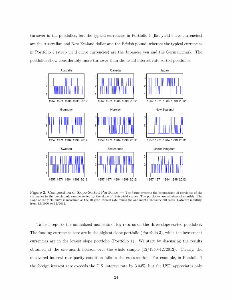
turnover in the portfolios, but the typical currencies in Portfolio 1 (flat yield curve currencies)

are the Australian and New Zealand dollar and the British pound, whereas the typical currencies

in Portfolio 3 (steep yield curve currencies) are the Japanese yen and the German mark. The

portfolios show considerably more turnover than the usual interest rate-sorted portfolios.

1957 1971 1984 1998 2012

1

2

3

Australia

1957 1971 1984 1998 2012

1

2

3

Canada

1957 1971 1984 1998 2012

1

2

3

Japan

1957 1971 1984 1998 2012

1

2

3

Germany

1957 1971 1984 1998 2012

1

2

3

Norway

1957 1971 1984 1998 2012

1

2

3

New Zealand

1957 1971 1984 1998 2012

1

2

3

Sweden

1957 1971 1984 1998 2012

1

2

3

Switzerland

1957 1971 1984 1998 2012

1

2

3

United Kingdom

Figure 2: Composition of Slope-Sorted Portfolios — The figure presents the composition of portfolios of thecurrencies in the benchmark sample sorted by the slope of their yield curves. The portfolios are rebalanced monthly. Theslope of the yield curve is measured as the 10-year interest rate minus the one-month Treasury bill rates. Data are monthly,from 12/1950 to 12/2012.

Table 1 reports the annualized moments of log returns on the three slope-sorted portfolios.

The funding currencies here are in the highest slope portfolio (Portfolio 3), while the investment

currencies are in the lowest slope portfolio (Portfolio 1). We start by discussing the results

obtained at the one-month horizon over the whole sample (12/1950–12/2012). Clearly, the

uncovered interest rate parity condition fails in the cross-section. For example, in Portfolio 1

the foreign interest rate exceeds the U.S. interest rate by 3.03%, but the USD appreciates only

24

by 0.01%. Average currency excess returns decline from 3.02% per annum on Portfolio 1 to

0.06% per annum on the Portfolio 3. Therefore, a long-short position of investing in steep-yield-

curve currencies and shorting flat-yield-curve currencies delivers an excess return of −2.97% per

annum and a Sharpe ratio of −0.47. Our findings confirm those of Ang and Chen (2010). The

slope of the yield curve predicts currency excess returns very well, implying that the entropy of

the temporary component plays a large role in currency risk premia.

As expected, Portfolio 3 produces large bond excess returns of 4% per annum, compared to

−1.82% per annum on Portfolio 1. Hence, a long-short position produces a spread of 5.82% per

annum.

A natural question is whether U.S. investors can “combine” this bond risk premium with

the currency risk premium. To answer this question, we compute the dollar bond excess returns

rx(10),$ by adding the currency excess returns rxFX and the local currency bond returns rx(10),∗.

In dollars, the aforementioned 5.82% spread is reduced to 2.85%, because of the partly offsetting

pattern in currency risk premia. What is driving these results? The low slope currencies tend

to be high interest rate currencies, while the high slope currencies tend to be low interest rate

currencies: Portfolio 1 has an interest rate difference of 3.03% relative to the U.S., while Portfolio

3 has a negative interest rate difference of −0.77% per annum. Thus, the flat slope currencies are

the investment currencies in the carry trade, whereas the steep slope currencies are the funding

currencies.

For long maturities, global bond investors want to reverse the standard currency carry trade.

They can achieve a return of 2.85% per annum by investing in the (low interest rate, steep curve)

funding currencies and shorting the (high interest rate, flat slope) carry trade currencies. This

difference is statistically significant. Importantly, this strategy involves long positions in bonds

issued by countries like Germany and Japan. These are countries with fairly liquid bond markets

and low sovereign credit risk. As a result, credit and liquidity risk differences are unlikely

candidate explanations for the return differences. Of course, at the one-month horizon, this

strategy involves frequent trading. At the 12-month horizon, these excess returns are essentially

gone. The local term premium almost fully offsets the carry trade premium.

25

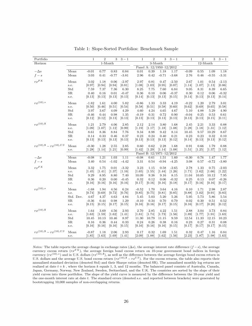
Table 1: Slope-Sorted Portfolios: Benchmark Sample

Portfolio 1 2 3 3− 1 1 2 3 3− 1 1 2 3 3− 1

Horizon 1-Month 3-Month 12-MonthPanel A: 12/1950–12/2012

−∆s Mean -0.01 0.77 0.83 0.84 0.01 0.39 1.18 1.17 -0.09 0.55 1.09 1.18f − s Mean 3.03 0.41 -0.77 -3.81 2.96 0.42 -0.71 -3.68 2.76 0.46 -0.55 -3.31

rxFX Mean 3.02 1.18 0.06 -2.97 2.97 0.81 0.47 -2.50 2.67 1.01 0.54 -2.13s.e. [0.97] [0.94] [0.94] [0.81] [1.08] [1.03] [0.95] [0.87] [1.14] [1.07] [1.13] [0.86]Std 7.59 7.37 7.36 6.30 8.25 7.75 7.60 6.84 9.05 8.31 8.39 6.65SR 0.40 0.16 0.01 -0.47 0.36 0.10 0.06 -0.37 0.30 0.12 0.06 -0.32s.e. [0.13] [0.13] [0.13] [0.13] [0.14] [0.13] [0.13] [0.15] [0.14] [0.13] [0.13] [0.14]

rx(10),∗ Mean -1.82 1.61 4.00 5.82 -0.86 1.33 3.33 4.19 -0.22 1.20 2.79 3.01s.e. [0.50] [0.46] [0.51] [0.54] [0.58] [0.51] [0.58] [0.60] [0.62] [0.69] [0.65] [0.58]Std 3.97 3.67 4.09 4.29 4.60 4.24 4.65 4.67 5.10 4.88 5.29 4.90SR -0.46 0.44 0.98 1.35 -0.19 0.31 0.72 0.90 -0.04 0.25 0.53 0.61s.e. [0.12] [0.12] [0.13] [0.13] [0.13] [0.13] [0.13] [0.13] [0.13] [0.13] [0.15] [0.11]

rx(10),$ Mean 1.21 2.79 4.06 2.85 2.12 2.14 3.80 1.68 2.45 2.21 3.33 0.88s.e. [1.09] [1.07] [1.12] [0.99] [1.19] [1.17] [1.18] [1.08] [1.28] [1.18] [1.31] [1.12]Std 8.61 8.36 8.84 7.76 9.34 8.98 9.42 8.14 10.45 9.57 10.29 8.67SR 0.14 0.33 0.46 0.37 0.23 0.24 0.40 0.21 0.23 0.23 0.32 0.10s.e. [0.13] [0.13] [0.13] [0.13] [0.13] [0.13] [0.13] [0.12] [0.14] [0.13] [0.13] [0.12]

rx(10),$ − rx(10),US Mean -0.30 1.28 2.55 2.85 0.60 0.62 2.28 1.68 0.91 0.66 1.79 0.88s.e. [1.28] [1.14] [1.21] [0.99] [1.42] [1.29] [1.14] [1.08] [1.51] [1.25] [1.37] [1.12]

Panel B: 12/1971–12/2012−∆s Mean -0.08 1.21 1.03 1.11 -0.08 0.61 1.51 1.60 -0.30 0.76 1.47 1.77f − s Mean 3.40 0.54 -1.02 -4.42 3.31 0.54 -0.94 -4.25 3.08 0.57 -0.72 -3.80

rxFX Mean 3.32 1.75 0.01 -3.32 3.23 1.15 0.58 -2.65 2.78 1.33 0.75 -2.03s.e. [1.45] [1.41] [1.37] [1.16] [1.65] [1.55] [1.44] [1.26] [1.71] [1.62] [1.66] [1.22]Std 9.29 8.95 8.80 7.40 10.09 9.38 9.16 8.15 11.04 10.05 10.12 7.95SR 0.36 0.20 0.00 -0.45 0.32 0.12 0.06 -0.32 0.25 0.13 0.07 -0.26s.e. [0.16] [0.16] [0.16] [0.16] [0.17] [0.16] [0.16] [0.18] [0.17] [0.16] [0.16] [0.17]

rx(10),∗ Mean -1.68 1.94 4.56 6.24 -0.52 1.70 3.64 4.16 0.10 1.71 2.98 2.87s.e. [0.74] [0.69] [0.72] [0.76] [0.85] [0.75] [0.81] [0.85] [0.88] [1.02] [0.91] [0.83]Std. Dev. 4.67 4.37 4.63 4.84 5.45 5.03 5.20 5.26 5.95 5.73 5.86 5.54SR -0.36 0.44 0.98 1.29 -0.10 0.34 0.70 0.79 0.02 0.30 0.51 0.52s.e. [0.15] [0.15] [0.17] [0.15] [0.16] [0.16] [0.17] [0.15] [0.16] [0.17] [0.20] [0.12]


rx(10),$ − rx(10),US Mean -0.87 1.18 2.06 2.93 0.17 0.32 1.69 1.51 0.32 0.47 1.16 0.84s.e. [1.85] [1.63] [1.69] [1.41] [2.09] [1.88] [1.62] [1.56] [2.23] [1.87] [1.98] [1.63]

Notes: The table reports the average change in exchange rates (∆s), the average interest rate difference (f −s), the averagecurrency excess return (rxFX), the average foreign bond excess return on 10-year government bond indices in foreigncurrency (rx(10),∗) and in U.S. dollars (rx(10),$), as well as the difference between the average foreign bond excess return inU.S. dollars and the average U.S. bond excess return (rx(10),$ − rxUS). For the excess returns, the table also reports theirannualized standard deviation (denoted Std) and their Sharpe ratios (denoted SR). The annualized monthly log returns arerealized at date t+ k , where the horizon k equals 1, 3, and 12 months. The balanced panel consists of Australia, Canada,Japan, Germany, Norway, New Zealand, Sweden, Switzerland, and the U.K. The countries are sorted by the slope of theiryield curves into three portfolios. The slope of the yield curve is measured by the difference between the 10-year yield andthe one-month interest rate at date t. The standard errors (denoted s.e. and reported between brackets) were generated bybootstrapping 10,000 samples of non-overlapping returns.

26

Our findings confirm that currency risk premia are driven to a large extent by temporary

shocks to the pricing kernel. When we sort currencies by the yield curve slope, roughly a measure

of the entropy of the temporary SDF component, we find large differences in currency risk premia:

the largest currency risk premia correspond to the lowest bond risk premia. This finding is

consistent with the theory, as total SDF entropy is negatively related to currency risk premia,

but positively related to bond risk premia. However, those differences in temporary pricing kernel

risk do not appear to produce significant cross-sectional differences in the quantity of permanent

risk: carry trade premia at the 10-year maturity, which are associated with differences in the

entropy of the permanent SDF component, are modest. Notably, the behavior of long-maturity

dollar bond returns suggests that local investors in carry trade countries are less exposed to

temporary risk than those in funding currencies, but more exposed to permanent risk.

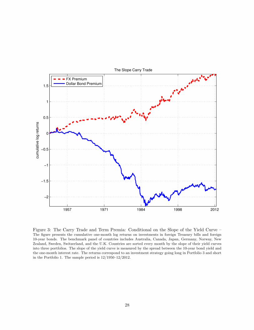
We get similar findings when we restrict our analysis to the post-Bretton Woods sample.

More generally, as can be verified from Figure 3 the difference in slope-sorted bond returns is

rather stable over time, although the difference in local bond premia is smaller in the last part

of the sample. For example, between 1991 and 2012, the difference in currency risk premia at

the one-month horizon between Portfolio 3 and Portfolio 1 is −4.20% per annum, compared to

a 3.29% spread in local term premia. This adds up to a −0.91% return on a long position in

the steep-sloped bonds and a short position in the flat-sloped bonds. However, this difference is

not statistically significant, as the standard error is 1.52% per annum.

Robustness Checks: Developed Countries and Whole Sample In the sample of devel-

oped countries, the steep-slope (low yielding) currencies are typically countries like Germany, the

Netherlands, Japan, and Switzerland, while the flat-slope (high-yielding) currencies are typically

Australia, New Zealand, Denmark and the U.K. At the one-month horizon, the 2.42% spread in

currency excess returns obtained in this sample is more than offset by the 5.90% spread in local

term premia. This produces a statistically significant 3.48% return on a position that is long

in the low yielding, high slope currencies and short in the high yielding, low slope currencies.

These results are essentially unchanged in the post-Bretton-Woods sample. At longer horizons,

the currency excess returns and the local risk premia almost fully offset each other.

27

1957 1971 1984 1998 2012

−2

−1.5

−1

−0.5

0

0.5

1

1.5

The Slope Carry Trade

cu

mula

tive log r

etu

rns

FX Premium

Dollar Bond Premium

Figure 3: The Carry Trade and Term Premia: Conditional on the Slope of the Yield Curve –The figure presents the cumulative one-month log returns on investments in foreign Treasury bills and foreign10-year bonds. The benchmark panel of countries includes Australia, Canada, Japan, Germany, Norway, NewZealand, Sweden, Switzerland, and the U.K. Countries are sorted every month by the slope of their yield curvesinto three portfolios. The slope of the yield curve is measured by the spread between the 10-year bond yield andthe one-month interest rate. The returns correspond to an investment strategy going long in Portfolio 3 and shortin the Portfolio 1. The sample period is 12/1950–12/2012.

28

In the entire sample of countries, including the emerging market countries, the difference in

currency risk premia in the 1-month horizon is 6.11% per annum, which is more than offset by

an 11.45% difference in local term premia. As a result, investors earn 5.33% per annum on a

long-short position in foreign bond portfolios of slope-sorted currencies. As before, this involves

shorting the flat-yield-curve currencies, typically high interest rate currencies, and going long in

the steep-slope currencies, typically the low interest rate ones. The annualized Sharpe ratio on

this long-short strategy is 0.60.

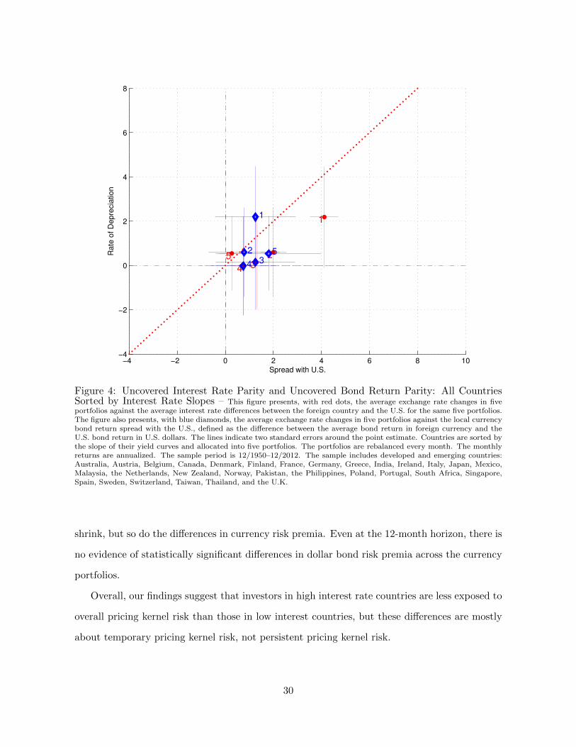
Figure 4 shows the deviations from the uncovered interest rate parity and long bond return

parity in the cross-section of the entire sample of countries. We form five currency portfolios. If

the UIP condition were a good description of the data, the red diamonds would be on the 45-

degree line. Notably, the biggest UIP violation occurs for Portfolio 1 (flat-yield-curve currencies),

for which high interest rates are not offset by an adequate rate of currency depreciation. If the

long-term bond return parity condition were a good description of the data, the blue dots would

be on the 45-degree line. In the data, the positive interest rate difference turns into a negative

bond return for the flat-slope portfolios (small dots), while the negative interest rate spread

becomes a positive return spread for the steep-slope bond portfolios (large dots).

3.3 Sorting Currencies by Interest Rates

Let us turn now to portfolios of countries sorted by their short-term interest rates. To save

space and because the results are very similar to those obtained on slope-sorted portfolios, we

summarize our findings rapidly here; detailed results are presented in the Online Appendix.

In our benchmark sample, as in our large samples, average currency excess returns increase

from low- to high-interest-rate portfolios. But local currency bond risk premia decrease from low-

to high-interest-rate portfolios. The decline in the local currency bond risk premia partly offsets

the increase in currency risk premia. As a result, the average excess return on the foreign bond

expressed in U.S. dollars measured in the high-interest-rate portfolio is only slightly higher than

the average excess returns measured in the low-interest-rate portfolio. As the holding period

increases from 1 to 3 and 12 months, the differences in local bond risk premia between portfolios

29

−4 −2 0 2 4 6 8 10−4

−2

0

2

4

6

8

1

234

5

1

234

5

Spread with U.S.

Rate

of D

epre

cia

tion

Figure 4: Uncovered Interest Rate Parity and Uncovered Bond Return Parity: All CountriesSorted by Interest Rate Slopes – This figure presents, with red dots, the average exchange rate changes in fiveportfolios against the average interest rate differences between the foreign country and the U.S. for the same five portfolios.The figure also presents, with blue diamonds, the average exchange rate changes in five portfolios against the local currencybond return spread with the U.S., defined as the difference between the average bond return in foreign currency and theU.S. bond return in U.S. dollars. The lines indicate two standard errors around the point estimate. Countries are sorted bythe slope of their yield curves and allocated into five portfolios. The portfolios are rebalanced every month. The monthlyreturns are annualized. The sample period is 12/1950–12/2012. The sample includes developed and emerging countries:Australia, Austria, Belgium, Canada, Denmark, Finland, France, Germany, Greece, India, Ireland, Italy, Japan, Mexico,Malaysia, the Netherlands, New Zealand, Norway, Pakistan, the Philippines, Poland, Portugal, South Africa, Singapore,Spain, Sweden, Switzerland, Taiwan, Thailand, and the U.K.

shrink, but so do the differences in currency risk premia. Even at the 12-month horizon, there is

no evidence of statistically significant differences in dollar bond risk premia across the currency

portfolios.

Overall, our findings suggest that investors in high interest rate countries are less exposed to

overall pricing kernel risk than those in low interest countries, but these differences are mostly

about temporary pricing kernel risk, not persistent pricing kernel risk.

30

3.4 The Term Structure of Currency Carry Trade Risk Premia

The previous results focus on the 10-year maturity and show that currency risk premia offset

local currency term premia for coupon bond returns. We now turn to a full set of returns in

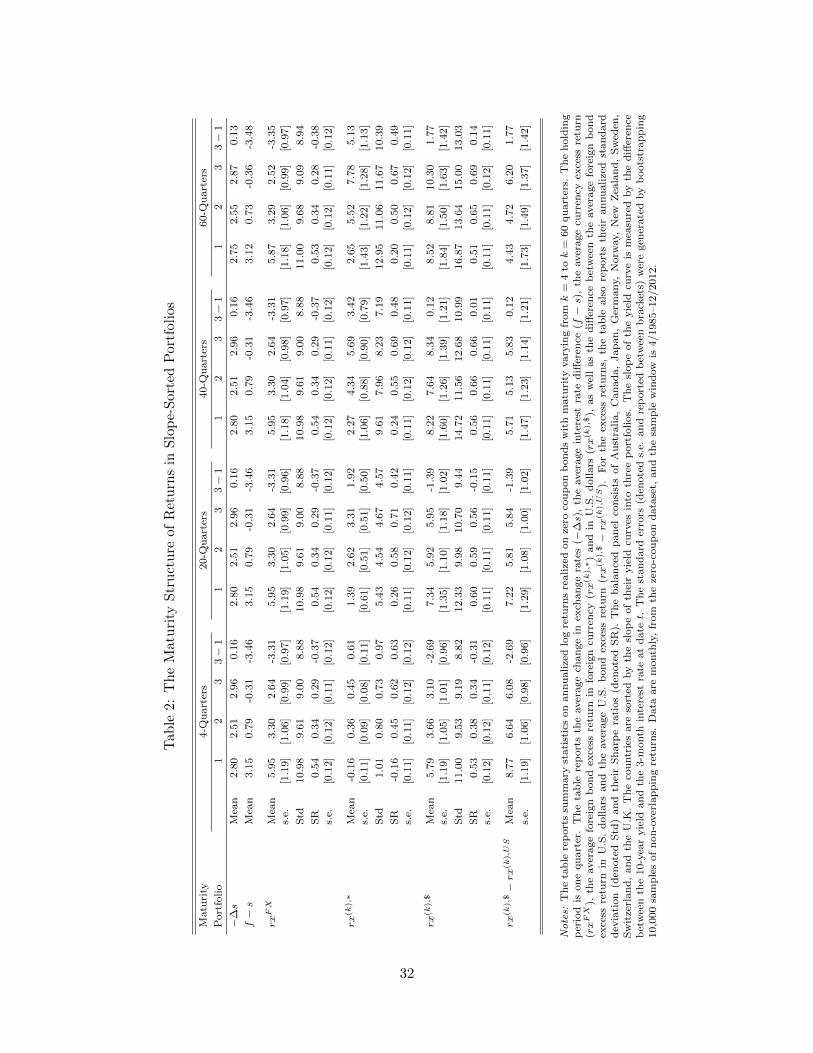
the maturity spectrum, using the zero-coupon bond dataset. Table 2 reports summary statistics

on one-quarter holding period returns on zero-coupon bond positions with maturities from 4 (1

year) to 60 quarters (15 years).

The term structure of currency carry trade risk premia is downward sloping: currency carry

trade strategies that yield positive risk premia for short-maturity bonds yield lower (or even

negative) risk premia for long-maturity bonds. This is due to the offsetting relationship between

currency premia and term premia. As we move from the 4-quarter maturity to the 60-quarter

maturity, the difference in the dollar term premium between Portfolio 1 (flat yield curve) cur-

rencies and Portfolio 3 (steep yield curve) currencies decreases from 2.69% to −1.77%. While

investing in flat yield curve currencies and shorting steep yield curve currencies provides signif-

icant gains in the short end of the term structure, it yields negative returns in the long end.

Figure 5 shows the local currency excess returns (in logs) in the top panel, and the dollar

excess returns (in logs) in the bottom panel. The top panel in Figure 5 shows that countries

with the steepest local yield curves (Portfolio 3, on the right-hand side) exhibit local bond excess

returns that are higher, and increase faster with the maturity than the flat yield curve countries

(Portfolio 1, on the left-hand side). This effect is strong enough to undo the effect of the level

differences in yields at the short end: the steep-slope currencies are typical funding currencies

with low yields in levels at the short end of the maturity curve while the flat-slope currencies

typically have high yields at the short end. At the 4-quarter maturity, Table 2 reports a −0.31%

interest rate difference with the U.S. in Portfolio 3, compared to a 3.15% interest rate difference

with the U.S. in Portfolio 1. Thus, ignoring the effect of exchange rates, investors should invest

in the bonds of steep yield curve currencies.

However, considering the effect of currency fluctuations by focusing on dollar returns radically

alters the results. Figure 5 shows that the dollar excess returns of Portfolio 1 are higher than

those of Portfolio 3 at the short maturity end, consistent with the carry trade results of Ang and

31

Tab

le2:

Th

eM

atu

rity

Str

uct

ure

ofR

etu

rns

inS

lop

e-S

orte

dP

ortf

olio

s

Matu

rity

4-Q

uart

ers

20-Q

uart

ers

40-Q

uart

ers

60-Q

uart

ers

Port

folio

12

33−

11

23

3−

11

23

3−

11

23

3−

1

−∆s

Mea

n2.8

02.5

12.9

60.1

62.8

02.5

12.9

60.1

62.8

02.5

12.9

60.1

62.7

52.5

52.8

70.1

3

f−s

Mea

n3.1

50.7

9-0

.31

-3.4

63.1

50.7

9-0

.31

-3.4

63.1

50.7

9-0

.31

-3.4

63.1

20.7

3-0

.36

-3.4

8

rxFX

Mea

n5.9

53.3

02.6

4-3

.31

5.9

53.3

02.6

4-3

.31

5.9

53.3

02.6

4-3

.31

5.8

73.2

92.5

2-3

.35

s.e.

[1.1

9]

[1.0

6]

[0.9

9]

[0.9

7]

[1.1

9]

[1.0

5]

[0.9

9]

[0.9

6]

[1.1

8]

[1.0

4]

[0.9

8]

[0.9

7]

[1.1

8]

[1.0

6]

[0.9

9]

[0.9

7]

Std

10.9

89.6

19.0

08.8

810.9

89.6

19.0

08.8

810.9

89.6

19.0

08.8

811.0

09.6

89.0

98.9

4

SR

0.5

40.3

40.2

9-0

.37

0.5

40.3

40.2

9-0

.37

0.5

40.3

40.2

9-0

.37

0.5

30.3

40.2

8-0

.38

s.e.

[0.1

2]

[0.1

2]

[0.1

1]

[0.1

2]

[0.1

2]

[0.1

2]

[0.1

1]

[0.1

2]

[0.1

2]

[0.1

2]

[0.1

1]

[0.1

2]

[0.1

2]

[0.1

2]

[0.1

1]

[0.1

2]

rx(k

),∗

Mea

n-0

.16

0.3

60.4

50.6

11.3

92.6

23.3

11.9

22.2

74.3

45.6

93.4

22.6

55.5

27.7

85.1

3s.

e.[0

.11]

[0.0

9]

[0.0

8]

[0.1

1]

[0.6

1]

[0.5

1]

[0.5

1]

[0.5

0]

[1.0

6]

[0.8

8]

[0.9

0]

[0.7

9]

[1.4

3]

[1.2

2]

[1.2

8]

[1.1

3]

Std

1.0

10.8

00.7

30.9

75.4

34.5

44.6

74.5

79.6

17.9

68.2

37.1

912.9

511.0

611.6

710.3

9

SR

-0.1

60.4

50.6

20.6

30.2

60.5

80.7

10.4

20.2

40.5

50.6

90.4

80.2

00.5

00.6

70.4

9s.

e.[0

.11]

[0.1

1]

[0.1

2]

[0.1

2]

[0.1

1]

[0.1

2]

[0.1

2]

[0.1

1]

[0.1

1]

[0.1

2]

[0.1

2]

[0.1

1]

[0.1

1]

[0.1

2]

[0.1

2]

[0.1

1]

rx(k

),$

Mea

n5.7

93.6

63.1

0-2

.69

7.3

45.9

25.9

5-1

.39

8.2

27.6

48.3

40.1

28.5

28.8

110.3

01.7

7s.

e.[1

.19]

[1.0

5]

[1.0

1]

[0.9

6]

[1.3

5]

[1.1

0]

[1.1

8]

[1.0

2]

[1.6

0]

[1.2

6]

[1.3

9]

[1.2

1]

[1.8

4]

[1.5

0]

[1.6

3]

[1.4

2]

Std

11.0

09.5

39.1

98.8

212.3

39.9

810.7

09.4

414.7

211.5

612.6

810.9

916.8

713.6

415.0

013.0

3

SR

0.5

30.3

80.3

4-0

.31

0.6

00.5

90.5

6-0

.15

0.5

60.6

60.6

60.0

10.5

10.6

50.6

90.1

4s.

e.[0

.12]

[0.1

2]

[0.1

1]

[0.1

2]

[0.1

1]

[0.1

1]

[0.1

1]

[0.1

1]

[0.1

1]

[0.1

1]

[0.1

1]

[0.1

1]

[0.1

1]

[0.1

1]

[0.1

2]

[0.1

1]

rx(k

),$−rx(k

),US

Mea

n8.7

76.6

46.0

8-2

.69

7.2

25.8

15.8

4-1

.39

5.7

15.1

35.8

30.1

24.4

34.7

26.2

01.7

7

s.e.

[1.1

9]

[1.0

6]

[0.9

8]

[0.9

6]

[1.2

9]

[1.0

8]

[1.0

0]

[1.0

2]

[1.4

7]

[1.2

3]

[1.1

4]

[1.2

1]

[1.7

3]

[1.4

9]

[1.3

7]

[1.4

2]

Notes:

Th

eta

ble

rep

ort

ssu

mm

ary

stati

stic

son

an

nu

alize

dlo

gre

turn

sre

ali

zed

on

zero

cou

pon

bon

ds

wit

hm

atu

rity

vary

ing

fromk

=4

tok

=60

qu

art

ers.

Th

eh

old

ing

per

iod

ison

equ

art

er.

Th

eta

ble

rep

ort

sth

eaver

age

chan

ge

inex

chan

ge

rate

s(−

∆s)

,th

eaver

age

inte

rest

rate

diff

eren

ce(f−s)

,th

eaver

age

curr

ency

exce

ssre

turn

(rxFX

),th

eaver

age

fore

ign

bon

dex

cess

retu

rnin

fore

ign

curr

ency

(rx(k

),∗)

an

din

U.S

.d

ollars

(rx(k

),$),

as

wel

las

the

diff

eren

ceb

etw

een

the

aver

age

fore

ign

bon

dex

cess

retu

rnin

U.S

.d

ollars

an

dth

eaver

age

U.S

.b

on

dex

cess

retu

rn(rx(k

),$−rx(k

),US

).F

or

the

exce

ssre

turn

s,th

eta

ble

als

ore

port

sth

eir

an

nu

alize

dst

an

dard

dev

iati

on

(den

ote

dS

td)

an

dth

eir

Sh

arp

era

tios

(den

ote

dS

R).

Th

eb

ala

nce

dp

an

elco

nsi

sts

of

Au

stra

lia,

Can

ad

a,

Jap

an

,G

erm

any,

Norw

ay,

New

Zea

lan

d,

Sw

eden

,S

wit

zerl

an

d,

an

dth

eU

.K.

Th

eco

untr

ies

are

sort

edby

the

slop

eof

thei

ryie

ldcu

rves

into

thre

ep

ort

folios.

Th

esl

op

eof

the

yie

ldcu

rve

ism

easu

red

by

the

diff

eren

ceb

etw

een

the

10-y

ear

yie

ldan

dth

e3-m

onth

inte

rest

rate

at

datet.

Th

est

an

dard

erro

rs(d

enote

ds.

e.an

dre

port

edb

etw

een

bra

cket

s)w

ere

gen

erate

dby

boots

trap

pin

g10,0

00

sam

ple

sof

non

-over

lap

pin

gre

turn

s.D

ata

are

month

ly,

from

the

zero

-cou

pon

data

set,

an

dth

esa

mp

lew

ind

ow

is4/1985–12/2012.

32

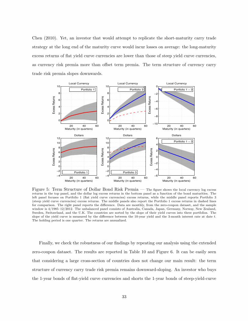
Chen (2010). Yet, an investor that would attempt to replicate the short-maturity carry trade

strategy at the long end of the maturity curve would incur losses on average: the long-maturity

excess returns of flat yield curve currencies are lower than those of steep yield curve currencies,

as currency risk premia more than offset term premia. The term structure of currency carry

trade risk premia slopes downwards.

Exc

ess

Ret

urns

Maturity (in quarters)

Local Currency

20 40 60

0

2

4

6

8

10

Portfolio 1

Exc

ess

Ret

urns


Local Currency

20 40 60

0

2

4

6

8

10

Portfolio 3

Exc

ess

Ret

urns


Local Currency

20 40 60−10

−8

−6

−4

−2

0

Portfolio 1 − 3

Exc

ess

Ret

urns


Dollars

20 40 60−4

−2

0

2

4

6

8

10

12

Portfolio 1

Exc

ess

Ret

urns


Dollars

20 40 60−4

−2

0

2

4

6

8

10

12

Portfolio 3

Exc

ess

Ret

urns


Dollars

20 40 60−6

−4

−2

0

2

4

6

Portfolio 1 − 3

Figure 5: Term Structure of Dollar Bond Risk Premia — The figure shows the local currency log excessreturns in the top panel, and the dollar log excess returns in the bottom panel as a function of the bond maturities. Theleft panel focuses on Portfolio 1 (flat yield curve currencies) excess returns, while the middle panel reports Portfolio 3(steep yield curve currencies) excess returns. The middle panels also report the Portfolio 1 excess returns in dashed linesfor comparison. The right panel reports the difference. Data are monthly, from the zero-coupon dataset, and the samplewindow is 4/1985–12/2012. The unbalanced panel consists of Australia, Canada, Japan, Germany, Norway, New Zealand,Sweden, Switzerland, and the U.K. The countries are sorted by the slope of their yield curves into three portfolios. Theslope of the yield curve is measured by the difference between the 10-year yield and the 3-month interest rate at date t.The holding period is one quarter. The returns are annualized.

Finally, we check the robustness of our findings by repeating our analysis using the extended

zero-coupon dataset. The results are reported in Table 10 and Figure 6. It can be easily seen

that considering a large cross-section of countries does not change our main result: the term

structure of currency carry trade risk premia remains downward-sloping. An investor who buys

the 1-year bonds of flat-yield curve currencies and shorts the 1-year bonds of steep-yield-curve

33

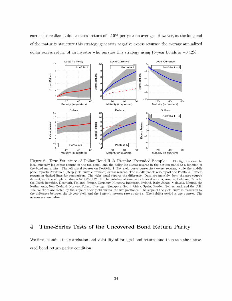
currencies realizes a dollar excess return of 4.10% per year on average. However, at the long end

of the maturity structure this strategy generates negative excess returns: the average annualized

dollar excess return of an investor who pursues this strategy using 15-year bonds is −0.42%.Ex

cess

Ret

urns


Local Currency

20 40 60

0

2

4

6

8

10Portfolio 1

Exce

ss R

etur

ns


Local Currency

20 40 60

0

2

4

6

8

10Portfolio 5

Exce

ss R

etur

ns


Dollars

20 40 60−4

−2

0

2

4

6

8

10

12

Portfolio 1

Exce

ss R

etur

ns


Dollars

20 40 60−4

−2

0

2

4

6

8

10

12

Portfolio 5

Exce

ss R

etur

ns


Local Currency

20 40 60−10

−8

−6

−4

−2

0Portfolio 1 − 5

Exce

ss R

etur

ns


Dollars

20 40 60−6

−4

−2

0

2

4

6Portfolio 1 − 5

Figure 6: Term Structure of Dollar Bond Risk Premia: Extended Sample — The figure shows thelocal currency log excess returns in the top panel, and the dollar log excess returns in the bottom panel as a function ofthe bond maturities. The left panel focuses on Portfolio 1 (flat yield curve currencies) excess returns, while the middlepanel reports Portfolio 5 (steep yield curve currencies) excess returns. The middle panels also report the Portfolio 1 excessreturns in dashed lines for comparison. The right panel reports the difference. Data are monthly, from the zero-coupondataset, and the sample window is 5/1987–12/2012. The unbalanced sample includes Australia, Austria, Belgium, Canada,the Czech Republic, Denmark, Finland, France, Germany, Hungary, Indonesia, Ireland, Italy, Japan, Malaysia, Mexico, theNetherlands, New Zealand, Norway, Poland, Portugal, Singapore, South Africa, Spain, Sweden, Switzerland, and the U.K.The countries are sorted by the slope of their yield curves into five portfolios. The slope of the yield curve is measured bythe difference between the 10-year yield and the 3-month interest rate at date t. The holding period is one quarter. Thereturns are annualized.

4 Time-Series Tests of the Uncovered Bond Return Parity

We first examine the correlation and volatility of foreign bond returns and then test the uncov-

ered bond return parity condition.

34

4.1 The Correlation and Volatility of Dollar Bond Returns

If international risk sharing is mostly due to countries sharing their permanent pricing kernel

fluctuations, holding period returns on zero-coupon bonds, once converted to a common cur-

rency (the U.S. dollar, in particular), should become increasingly similar as bond maturities

approach infinity. To determine whether this hypothesis has merit, Figure 7 reports the cor-

relation coefficient between three-month returns on foreign zero-coupon bonds (either in local

currency or in U.S. dollars) and corresponding returns on U.S. bonds for bonds of maturity

ranging from 1 year to 15 years. All foreign currency yield curves exhibit the same pattern:

correlation coefficients for U.S. dollar returns start from very low (often negative) values and

increase monotonically with bond maturity, tending towards one for long-term bonds. The clear

monotonicity is not observed on local currency returns. The local currency three-month return

correlations do not exhibit any discernible pattern with maturity, implying that the convergence

of U.S. dollar return correlations towards the value of one results from exchange rate changes

that partially offset differences in local currency bond returns. Similar results hold true for

volatility ratios (instead of correlations); we report those in the Online Appendix.

In sum, the behavior of U.S. dollar bond returns and local currency bond returns differs

markedly as bond maturity changes. While U.S. dollar bond returns become more correlated

and roughly equally volatile across countries as the maturity increases, the behavior of local

currency returns do not appear to change when bond maturity changes.

4.2 Testing Uncovered Bond Return Parity in the Time-Series

We now turn to tests of the bond return parity condition in the time series. To the extent the

10-year bond is a reasonable proxy for the infinite-maturity bond, uncovered long-bond parity

implies that the domestic and foreign 10-year bond returns are not statistically different across

countries, once converted into a common currency. To determine whether exchange rate changes

completely eliminate differences in countries’ permanent SDF components, nominal U.S. dollar

holding period returns on 10-year foreign bonds are thus regressed on the corresponding U.S.

35

5 10 15

0

0.5

1Australia

Maturity (in years)

Cor

rela

tion

coef

ficie

nt

LocalUSD

5 10 15

0

0.5

1Canada

Maturity (in years)

Cor

rela

tion

coef

ficie

nt

5 10 15

0

0.5

1Germany

Maturity (in years)

Cor

rela

tion

coef

ficie

nt

5 10 15

0

0.5

1Japan

Maturity (in years)

Cor

rela

tion

coef

ficie

nt

5 10 15

0

0.5

1New Zealand

Maturity (in years)

Cor

rela

tion

coef

ficie

nt

5 10 15

0

0.5

1Norway

Maturity (in years)

Cor

rela

tion

coef

ficie

nt5 10 15

0

0.5

1Sweden

Maturity (in years)

Cor

rela

tion

coef

ficie

nt

5 10 15

0

0.5

1Switzerland

Maturity (in years)

Cor

rela

tion

coef

ficie

nt

5 10 15

0

0.5

1United Kingdom

Maturity (in years)

Cor

rela

tion

coef

ficie

nt

Figure 7: The Maturity Structure of Bond Return Correlations — The figure presents the correlationof foreign bond returns with U.S. bond returns. The time-window is country-dependent. Data are monthly. The holdingperiod is three-months.

dollar returns on 10-year U.S. bonds:

r(10),$t+1 = α+ βr

(10)t+1 + εt+1,

where small letters denote the log of their capital letter counterpart. Uncovered long bond

parity implies α = 0 and β = 1. Table 3 also reports regressions results obtained with each

component of the dollar return, i.e., the local currency bond return r(10),∗t+1 and the change in the

log exchange rate, as well as total returns. The sum of the local currency bond return beta and

the exchange change beta equals the total dollar bond return beta. Section I of Table 3 uses

discount bonds, while Section II uses zero-coupon bonds.

36

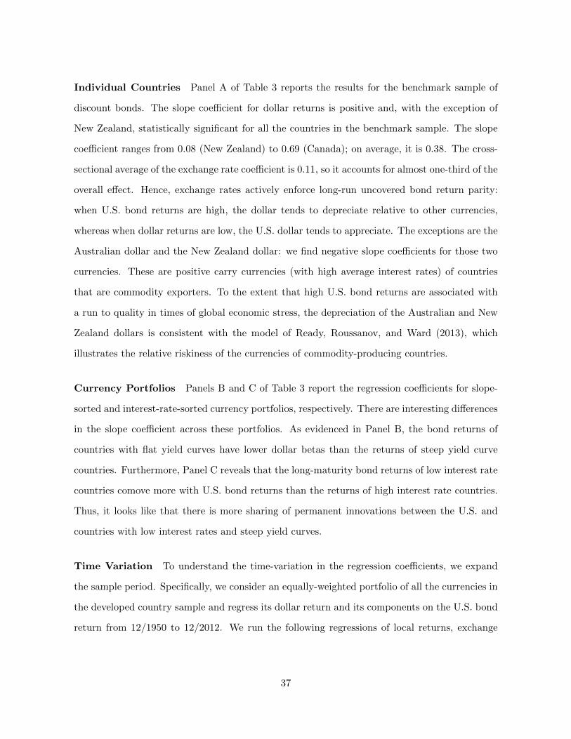
Individual Countries Panel A of Table 3 reports the results for the benchmark sample of

discount bonds. The slope coefficient for dollar returns is positive and, with the exception of

New Zealand, statistically significant for all the countries in the benchmark sample. The slope

coefficient ranges from 0.08 (New Zealand) to 0.69 (Canada); on average, it is 0.38. The cross-

sectional average of the exchange rate coefficient is 0.11, so it accounts for almost one-third of the

overall effect. Hence, exchange rates actively enforce long-run uncovered bond return parity:

when U.S. bond returns are high, the dollar tends to depreciate relative to other currencies,

whereas when dollar returns are low, the U.S. dollar tends to appreciate. The exceptions are the

Australian dollar and the New Zealand dollar: we find negative slope coefficients for those two

currencies. These are positive carry currencies (with high average interest rates) of countries

that are commodity exporters. To the extent that high U.S. bond returns are associated with

a run to quality in times of global economic stress, the depreciation of the Australian and New

Zealand dollars is consistent with the model of Ready, Roussanov, and Ward (2013), which

illustrates the relative riskiness of the currencies of commodity-producing countries.

Currency Portfolios Panels B and C of Table 3 report the regression coefficients for slope-

sorted and interest-rate-sorted currency portfolios, respectively. There are interesting differences

in the slope coefficient across these portfolios. As evidenced in Panel B, the bond returns of

countries with flat yield curves have lower dollar betas than the returns of steep yield curve

countries. Furthermore, Panel C reveals that the long-maturity bond returns of low interest rate

countries comove more with U.S. bond returns than the returns of high interest rate countries.

Thus, it looks like that there is more sharing of permanent innovations between the U.S. and

countries with low interest rates and steep yield curves.

Time Variation To understand the time-variation in the regression coefficients, we expand

the sample period. Specifically, we consider an equally-weighted portfolio of all the currencies in

the developed country sample and regress its dollar return and its components on the U.S. bond

return from 12/1950 to 12/2012. We run the following regressions of local returns, exchange

37

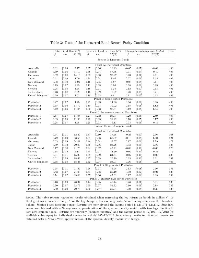
Table 3: Tests of the Uncovered Bond Return Parity Condition

Return in dollars (r$) Return in local currency (r∗) Change in exchange rate (−∆s) Obs.

β s.e. R2(%) β s.e. R2(%) β s.e. R2(%)

Section I: Discount Bonds

Panel A: Individual Countries

Australia 0.32 [0.08] 3.77 0.37 [0.06] 16.93 -0.05 [0.07] -0.08 493

Canada 0.69 [0.06] 31.19 0.68 [0.04] 57.58 0.01 [0.04] -0.19 493

Germany 0.62 [0.08] 14.16 0.38 [0.03] 25.97 0.23 [0.07] 2.61 493

Japan 0.51 [0.09] 8.09 0.24 [0.04] 8.46 0.27 [0.06] 3.55 493

New Zealand 0.08 [0.10] -0.02 0.16 [0.05] 1.87 -0.08 [0.08] 0.11 493

Norway 0.19 [0.07] 1.83 0.11 [0.03] 3.06 0.08 [0.06] 0.23 493

Sweden 0.28 [0.08] 3.55 0.16 [0.04] 5.25 0.12 [0.07] 0.63 493

Switzerland 0.43 [0.08] 7.39 0.15 [0.02] 15.97 0.28 [0.08] 3.21 493

United Kingdom 0.29 [0.07] 4.02 0.18 [0.03] 8.81 0.11 [0.07] 0.62 493

Panel B: Slope-sorted Portfolios

Portfolio 1 0.27 [0.07] 4.45 0.21 [0.03] 14.38 0.06 [0.06] 0.05 493

Portfolio 2 0.45 [0.06] 13.79 0.30 [0.03] 30.02 0.15 [0.06] 1.82 493

Portfolio 3 0.42 [0.06] 11.05 0.30 [0.03] 28.31 0.12 [0.05] 1.04 493

Panel C: Interest-rate-sorted Portfolios

Portfolio 1 0.47 [0.07] 11.98 0.27 [0.02] 28.97 0.20 [0.06] 2.89 493

Portfolio 2 0.39 [0.05] 11.90 0.29 [0.03] 29.92 0.10 [0.05] 0.77 493

Portfolio 3 0.28 [0.07] 4.48 0.25 [0.03] 16.13 0.03 [0.06] -0.15 493

Section II: Zero-Coupon Bonds

Panel A: Individual Countries

Australia 0.54 [0.11] 12.39 0.77 [0.10] 37.78 -0.23 [0.07] 2.96 308

Canada 0.72 [0.09] 33.56 0.81 [0.06] 65.07 -0.10 [0.05] 1.30 321

Germany 0.63 [0.08] 24.21 0.46 [0.04] 37.57 0.17 [0.06] 2.79 477

Japan 0.69 [0.12] 20.00 0.36 [0.06] 21.76 0.33 [0.09] 7.36 333

New Zealand 0.77 [0.10] 21.76 0.84 [0.07] 45.21 -0.08 [0.10] -0.03 273

Norway 0.38 [0.12] 5.81 0.44 [0.07] 18.70 -0.06 [0.14] -0.37 177

Sweden 0.61 [0.11] 15.39 0.68 [0.09] 34.34 -0.07 [0.10] -0.09 238

Switzerland 0.61 [0.09] 18.43 0.37 [0.05] 25.79 0.23 [0.10] 3.01 297

United Kingdom 0.58 [0.08] 18.44 0.52 [0.07] 28.97 0.06 [0.06] 0.22 405

Panel B: Slope-sorted Portfolios

Portfolio 1 0.68 [0.11] 21.22 0.56 [0.07] 32.98 0.12 [0.08] 0.96 333

Portfolio 2 0.53 [0.07] 21.03 0.51 [0.06] 39.19 0.02 [0.07] -0.24 333

Portfolio 3 0.74 [0.07] 35.03 0.57 [0.06] 47.61 0.17 [0.08] 3.35 333

Panel C: Interest-rate-sorted Portfolios

Portfolio 1 0.70 [0.09] 28.34 0.44 [0.05] 40.44 0.26 [0.07] 6.81 333

Portfolio 2 0.70 [0.07] 32.73 0.60 [0.07] 51.72 0.10 [0.09] 0.88 333

Portfolio 3 0.60 [0.09] 20.76 0.60 [0.07] 39.94 0.00 [0.08] -0.30 333

Notes: The table reports regression results obtained when regressing the log return on bonds in dollars r$, orthe log return in local currency r∗, or the log change in the exchange rate ∆s on the log return on U.S. bonds indollars. Section I uses discount bonds. Returns are monthly and the sample period is 12/1971–12/2012. Standarderrors are obtained with a Newey-West approximation of the spectral density matrix with two lags. Section IIuses zero-coupon bonds. Returns are quarterly (sampled monthly) and the sample period is 12/1971–12/2012 (oravailable subsample) for individual currencies and 4/1985–12/2012 for currency portfolios. Standard errors areobtained with a Newey-West approximation of the spectral density matrix with 6 lags.

38

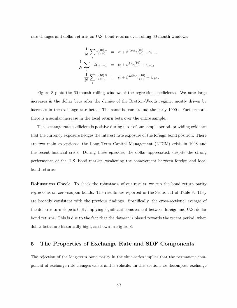
rate changes and dollar returns on U.S. bond returns over rolling 60-month windows:

1

N

∑i

r(10),∗i,t+1 = α+ βlocalr

(10)t+1 + εt+1,

1

N

∑i

−∆si,t+1 = α+ βfxr(10)t+1 + εt+1,

1

N

∑i

r(10),$i,t+1 = α+ βdollarr

(10)t+1 + εt+1.

Figure 8 plots the 60-month rolling window of the regression coefficients. We note large

increases in the dollar beta after the demise of the Bretton-Woods regime, mostly driven by

increases in the exchange rate betas. The same is true around the early 1990s. Furthermore,

there is a secular increase in the local return beta over the entire sample.

The exchange rate coefficient is positive during most of our sample period, providing evidence

that the currency exposure hedges the interest rate exposure of the foreign bond position. There

are two main exceptions: the Long Term Capital Management (LTCM) crisis in 1998 and

the recent financial crisis. During these episodes, the dollar appreciated, despite the strong

performance of the U.S. bond market, weakening the comovement between foreign and local

bond returns.

Robustness Check To check the robustness of our results, we run the bond return parity

regressions on zero-coupon bonds. The results are reported in the Section II of Table 3. They

are broadly consistent with the previous findings. Specifically, the cross-sectional average of

the dollar return slope is 0.61, implying significant comovement between foreign and U.S. dollar

bond returns. This is due to the fact that the dataset is biased towards the recent period, when

dollar betas are historically high, as shown in Figure 8.

5 The Properties of Exchange Rate and SDF Components

The rejection of the long-term bond parity in the time-series implies that the permanent com-

ponent of exchange rate changes exists and is volatile. In this section, we decompose exchange

39

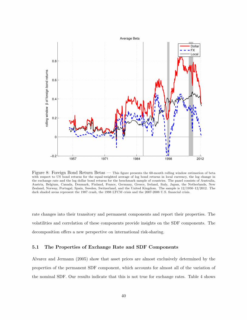
1957 1971 1984 1998 2012−0.2

0

0.2

0.4

0.6

0.8

rolli

ng w

indow

β o

f fo

reig

n b

ond r

etu

rns

Average Beta

Dollar

FX

Local

Figure 8: Foreign Bond Return Betas — This figure presents the 60-month rolling window estimation of betawith respect to US bond returns for the equal-weighted average of log bond returns in local currency, the log change inthe exchange rate and the log dollar bond returns for the benchmark sample of countries. The panel consists of Australia,Austria, Belgium, Canada, Denmark, Finland, France, Germany, Greece, Ireland, Italy, Japan, the Netherlands, NewZealand, Norway, Portugal, Spain, Sweden, Switzerland, and the United Kingdom. The sample is 12/1950–12/2012. Thedark shaded areas represent the 1987 crash, the 1998 LTCM crisis and the 2007-2008 U.S. financial crisis.

rate changes into their transitory and permanent components and report their properties. The

volatilities and correlation of these components provide insights on the SDF components. The

decomposition offers a new perspective on international risk-sharing.

5.1 The Properties of Exchange Rate and SDF Components

Alvarez and Jermann (2005) show that asset prices are almost exclusively determined by the

properties of the permanent SDF component, which accounts for almost all of the variation of

the nominal SDF. Our results indicate that this is not true for exchange rates. Table 4 shows

40

that the internationally unshared parts of the two components of the nominal SDF contribute

roughly equally to the volatility of the nominal SDF. The annualized volatility of the 3-month

exchange rate changes ranges from 7% to 12%. Although the two exchange rate components

contribute to exchange rate volatility about equally, the transitory component tends to be the

relatively smoother component, with its volatility ranging from 6% to 12%. The permanent

component is slightly more volatile than the overall exchange rate, ranging in volatility from

10% to 16%.

The two components are negatively correlated for all exchange rates. Across the countries

of the benchmark sample, the unconditional correlation of the two exchange rate components

ranges from -0.38 to -0.73. In unreported results, a similar decomposition of 6-month and 12-

month exchange rate changes produces quantitatively similar results. This implies that changes

in the unshared part of the permanent, asset-pricing component of the SDF are partly offset

by changes in the unshared part of the transitory component. This offsetting does not affect

asset prices, since the permanent SDF component is an order of magnitude larger than the

transitory component. However, it can potentially have large effects in the behavior of exchange

rates, as the size of the internationally non-shared parts of the two SDF components does not

differ much. Cross-sectionally, the correlation between overall exchange rate changes and their

transitory component ranges from -0.14 to 0.30, whereas the correlation between exchange rate

changes and their permanent component is much higher, ranging from 0.68 to 0.81.

In unreported results, proxying the infinite maturity bond with the 15-year bond delivers

substantially similar findings, indicating that our results are robust to alternative proxies for

the infinite maturity bond.

5.2 The Implications for International Risk Sharing

Our findings imply that fluctuations in the permanent SDF component are internationally shared

to a significantly larger extent than fluctuations in the transitory SDF component. For each

country’s transitory SDF component, we calculate the annualized standard deviation and the

correlation coefficient with the transitory component of the U.S. SDF and report the results in

41

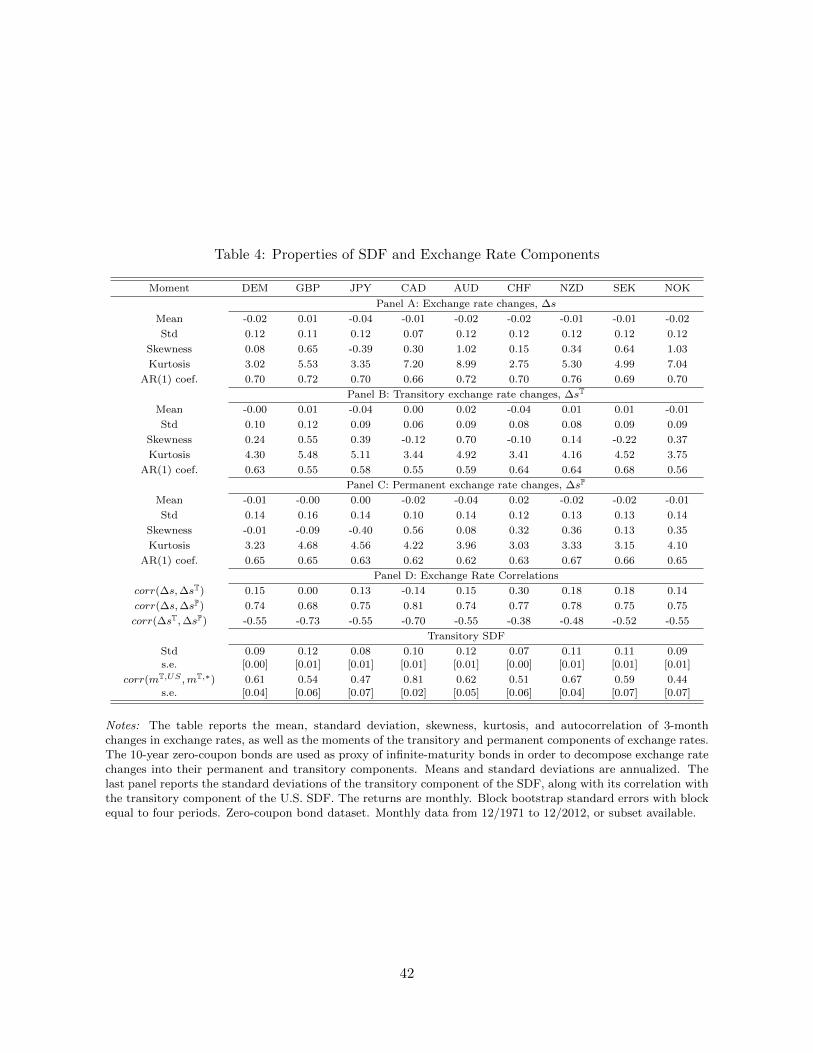
Table 4: Properties of SDF and Exchange Rate Components

Moment DEM GBP JPY CAD AUD CHF NZD SEK NOK

Panel A: Exchange rate changes, ∆s

Mean -0.02 0.01 -0.04 -0.01 -0.02 -0.02 -0.01 -0.01 -0.02

Std 0.12 0.11 0.12 0.07 0.12 0.12 0.12 0.12 0.12

Skewness 0.08 0.65 -0.39 0.30 1.02 0.15 0.34 0.64 1.03

Kurtosis 3.02 5.53 3.35 7.20 8.99 2.75 5.30 4.99 7.04

AR(1) coef. 0.70 0.72 0.70 0.66 0.72 0.70 0.76 0.69 0.70

Panel B: Transitory exchange rate changes, ∆sT

Mean -0.00 0.01 -0.04 0.00 0.02 -0.04 0.01 0.01 -0.01

Std 0.10 0.12 0.09 0.06 0.09 0.08 0.08 0.09 0.09

Skewness 0.24 0.55 0.39 -0.12 0.70 -0.10 0.14 -0.22 0.37

Kurtosis 4.30 5.48 5.11 3.44 4.92 3.41 4.16 4.52 3.75

AR(1) coef. 0.63 0.55 0.58 0.55 0.59 0.64 0.64 0.68 0.56

Panel C: Permanent exchange rate changes, ∆sP

Mean -0.01 -0.00 0.00 -0.02 -0.04 0.02 -0.02 -0.02 -0.01

Std 0.14 0.16 0.14 0.10 0.14 0.12 0.13 0.13 0.14

Skewness -0.01 -0.09 -0.40 0.56 0.08 0.32 0.36 0.13 0.35

Kurtosis 3.23 4.68 4.56 4.22 3.96 3.03 3.33 3.15 4.10

AR(1) coef. 0.65 0.65 0.63 0.62 0.62 0.63 0.67 0.66 0.65

Panel D: Exchange Rate Correlations

corr(∆s,∆sT) 0.15 0.00 0.13 -0.14 0.15 0.30 0.18 0.18 0.14

corr(∆s,∆sP) 0.74 0.68 0.75 0.81 0.74 0.77 0.78 0.75 0.75

corr(∆sT,∆sP) -0.55 -0.73 -0.55 -0.70 -0.55 -0.38 -0.48 -0.52 -0.55

Transitory SDF

Std 0.09 0.12 0.08 0.10 0.12 0.07 0.11 0.11 0.09s.e. [0.00] [0.01] [0.01] [0.01] [0.01] [0.00] [0.01] [0.01] [0.01]

corr(mT,US ,mT,∗) 0.61 0.54 0.47 0.81 0.62 0.51 0.67 0.59 0.44s.e. [0.04] [0.06] [0.07] [0.02] [0.05] [0.06] [0.04] [0.07] [0.07]

Notes: The table reports the mean, standard deviation, skewness, kurtosis, and autocorrelation of 3-monthchanges in exchange rates, as well as the moments of the transitory and permanent components of exchange rates.The 10-year zero-coupon bonds are used as proxy of infinite-maturity bonds in order to decompose exchange ratechanges into their permanent and transitory components. Means and standard deviations are annualized. Thelast panel reports the standard deviations of the transitory component of the SDF, along with its correlation withthe transitory component of the U.S. SDF. The returns are monthly. Block bootstrap standard errors with blockequal to four periods. Zero-coupon bond dataset. Monthly data from 12/1971 to 12/2012, or subset available.

42

Table 4. We also report the bootstrap standard error for each moment.

Table 4 shows that for all countries, the annualized standard deviation of the transitory

SDF component is significantly smaller than the typically calculated Hansen-Jagannathan lower

bound of total SDF volatility. For the 3-month pricing kernel changes, the volatility ranges from

7% (for Switzerland) to 12% (for a number of countries), whereas conventional estimates of the

SDF lower bound exceed 50%. Those results are consistent with the Alvarez and Jermann (2005)

findings that the transitory SDF component is second-order. However, by Brandt, Cochrane, and

Santa-Clara (2006) logic, the much smaller volatility of the transitory SDF component, coupled

with the fact that the transitory component of exchange rate changes is about as volatile as the

total exchange rate changes, implies that the cross-country correlation of the transitory SDF

component is significantly lower than the cross-country correlation of the overall SDF. Indeed,

the last panel of Table 4 reports that, for 3-month pricing kernel changes, correlations range from

0.44 (between the U.S. and Norway) to 0.81 (between the U.S. and Canada). Those correlation

coefficients represent much smaller common variation than the almost perfectly correlated SDFs

reported in Brandt, Cochrane, and Santa-Clara (2006). It follows that there is much more

internationally common variation regarding the permanent SDF component than the transitory

SDF component. In unreported results, we find that our conclusions are robust for six-month

and 12-month pricing kernel changes.

6 Conclusion

In this paper, we derive a novel uncovered bond return parity condition. If permanent shocks

to the pricing kernels are perfectly shared, then long-term bond returns, once expressed in a

common currency, should be equalized across countries. If permanent shocks are not perfectly

shared, then the difference between the domestic and foreign long-term bond risk premia, again

expressed in a common currency, reflects the difference in the entropy of the permanent com-

ponents of the stochastic discount factor. Our results are preference-free and rely only on the

absence of arbitrage.

In the cross-section, we find that the term structure of currency risk premia is downward

43

sloping. While carry trade strategies based on the three-month Treasury bills are highly prof-

itable, carry trade strategies using long-maturity bonds are not. On average, the excess returns

obtained by going long bonds in high interest rate currencies and short in low interest rate cur-

rencies do not offer significant excess returns. The same is true for investment strategies that go

long in countries whose yield curves are flat and short in countries whose yield curves are steep.

The downward-sloping term structure of carry trade risk premia implies that the permanent

component of the stochastic discount factor has similar entropy across countries. While Alvarez

and Jermann (2005) find that domestic equity and bond markets’ risk premia imply that the

pricing kernel is mostly driven by permanent shocks, our findings suggest that a large share of

these permanent shocks is already well-shared across countries. We confirm this insight in the

time-series by decomposing exchange rate changes into a component that reflects cross-country

differences in permanent pricing kernel innovations and one that encodes differences in transitory

innovations. It appears that the shocks not shared in international financial markets are much

less persistent than the overall shocks driving pricing kernels in asset markets.

44

References

Alvarez, F., and U. J. Jermann (2004): “Using Asset Prices to Measure the Cost of Business

Cycles,” Journal of Political Economy, 112(6), 1123–1256.

(2005): “Using Asset Prices to Measure the Persistence of the Marginal Utility of

Wealth,” Econometrica, 73(6), 1977–2016.

Ang, A., and J. S. Chen (2010): “Yield Curve Predictors of Foreign Exchange Returns,”

Working Paper, Columbia University.

Backus, D., M. Chernov, and S. Zin (2012): “Sources of entropy in representative agent

models,” Journal of Finance, forthcoming.

Backus, D., S. Foresi, and C. Telmer (2001): “Affine Models of Currency Pricing: Ac-

counting for the Forward Premium Anomaly,” Journal of Finance, 56, 279–304.

Bakshi, G., and F. Chabi-Yo (2012): “Variance bounds on the permanent and transitory

components of stochastic discount factors,” Journal of Financial Economics, 105, 191–208.

Bansal, R. (1997): “An Exploration of the Forward Premium Puzzle in Currency Markets,”

Review of Financial Studies, 10, 369–403.

Bansal, R., and B. N. Lehmann (1997): “Growth Optimal Portfolio Restrictions on Asset

Pricing Models,” Macroeconomic Dynamics, 1, 333–354.

Bekaert, G. (1996): “The Time Variation of Risk and Return in Foreign Exchange Markets:

A General Equilibrium Perspective,” The Review of Financial Studies, 9(2), 427–470.

Borovicka, J., L. P. Hansen, M. Hendricks, and J. A. Scheinkman (2011): “Risk Price

Dynamics,” Journal of Financial Econometrics, 9(1), 3–65.

Boudoukh, J., M. Richardson, and R. F. Whitelaw (2013): “New Evidence on the

Forward Premium Puzzle,” Working Paper, NYU.

45

Brandt, M. W., J. H. Cochrane, and P. Santa-Clara (2006): “International Risk Shar-

ing is Better Than You Think, or Exchange Rates are Too Smooth,” Journal of Monetary

Economics, 53(4), 671 – 698.

Brunnermeier, M. K., S. Nagel, and L. H. Pedersen (2009): “Carry Trades and Currency

Crashes,” NBER Macroeconomics Annual 2008, 23, 313–347.

Campbell, J. Y., and R. J. Shiller (1991): “Yield Spreads and Interest Rate Movements:

A Bird’s Eye View,” Review of Economic Studies, 58, 495–514.

Chernov, M., J. Graveline, and I. Zviadadze (2011): “Sources of Risk in Currency Re-

turns,” Working Paper, London School of Economics.

Chinn, M. D., and G. Meredith (2004): “Monetary Policy and Long-Horizon Uncovered

Interest Parity,” IMF Staff Papers, 51(3), 409–430.

Coeurdacier, N., H. Rey, and P. Winant (2013): “Financial Integration and Growth in a

Risky World,” Working Paper, London Business School.

Colacito, R., and M. M. Croce (2011): “Risks for the Long Run and the Real Exchange

Rate,” Journal of Political Economy, 119(1), 153–181.

Cole, H. L., and M. Obstfeld (1991): “Commodity Trade and International Risk Sharing:

How Much Do Financial Markets Matter?,” Journal of Monetary Economics, 28(1), 3–24.

Cox, J. C., J. E. Ingersoll, and S. A. Ross (1985): “A Theory of the Term Structure of

Interest Rates,” Econometrica, 53(2), 385–408.

Dahlquist, M., and H. Hasseltoft (2013): “International Bond Risk Premia,” Journal of

International Economics, 90, 12–32.

Engel, C. (1996): “The Forward Discount Anomaly and the Risk Premium: A Survey of

Recent Evidence,” Journal of Empirical Finance, 3, 123–192.

Farhi, E., S. P. Fraiberger, X. Gabaix, R. Ranciere, and A. Verdelhan (2013):

“Crash Risk in Currency Markets,” Working Paper, Harvard University.

46

Gavazzoni, F., B. Sambalaibat, and C. Telmer (2012): “Currency Risk and Pricing Kernel

Volatility,” Working Paper, Carnegie Mellon University.

Gourinchas, P.-O., and O. Jeanne (2006): “The elusive gains from international financial

integration,” The Review of Economic Studies, 73(3), 715–741.

Gourio, F., M. Siemer, and A. Verdelhan (2013): “International Risk Cycles,” Journal of

International Economics, 89, 471–484.

Hansen, L. P. (2009): “Modeling the Long Run: Valuation in Dynamic Stochastic Economies,”

Fisher-Schultz Lecture at the European Meetings of the Econometric Society.

Hansen, L. P., J. C. Heaton, and N. Li (2008): “Consumption Strikes Back? Measuring

Long-Run Risk,” Journal of Political Economy, 166(2), 260–302.

Hansen, L. P., and J. A. Scheinkman (2009): “Long-Term Risk: An Operator Approach,”

Econometrica, 77(1), 177–234.

Jotikasthira, C., A. Le, and C. Lundblad (2012): “Why Do Term Structures in Different

Currencies Comove?,” Working Paper, University of North Carolina.

Jurek, J. W. (2008): “Crash-neutral Currency Carry Trades,” Working Paper, Princeton

University.

Koijen, R., T. J. Moskowitz, L. H. Pedersen, and E. B. Vrugt (2012): “Carry,” Working

Paper, University of Chicago.

Lewis, K. K. (2000): “Why Do Stocks and Consumption Imply Such Different Gains From

International Risk-Sharing?,” Journal of International Economics, 52(1), 1–35.

Lewis, K. K. (2011): “Global Asset Pricing,” Annual Review of Financial Economics.

Lewis, K. K., and E. X. Liu (2012): “Evaluating International Consumption Risk Sharing

Gains: An Asset Return View,” Working Paper, University of Pennsylvania.

47

Lustig, H., N. Roussanov, and A. Verdelhan (2011): “Common Risk Factors in Currency

Returns,” Review of Financial Studies, 24(11).

Lustig, H., and A. Verdelhan (2007): “The Cross-Section of Foreign Currency Risk Premia

and Consumption Growth Risk,” American Economic Review, 97(1), 98–117.

Martin, I., and S. A. Ross (2013): “The Long Bond,” Working Paper, Stanford University.

Menkhoff, L., L. Sarno, M. Schmeling, and A. Schrimpf (2012): “Carry Trades and

Global FX Volatility,” Journal of Finance, 67(2), 681–718.

Ready, R. C., N. L. Roussanov, and C. Ward (2013): “Commodity Trade and the Carry

Trade: A Tale of Two Countries,” Working Paper, University of Pennsylvania.

Ross, S. (2013): “The Recovery Theorem,” Journal of Finance, forthcoming.

Wincoop, E. v. (1994): “Welfare Gains From International Risk-Sharing,” Journal of Mone-

tary Economics, 34(2), 175–200.

Wright, J. H. (2011): “Term Premia and Inflation Uncertainty: Empirical Evidence from an

International Panel Dataset,” American Economic Review, 101, 1514–1534.

Wu, L. J. (2012): “Global Yield Curve Risk Factors in International Bond and Currency

Portfolios,” Working Paper, UCLA.

48

Online Appendix for “The Term Structureof Currency Carry Trade Risk Premia”

—Not For Publication—

Section A reports the proofs of the theoretical results presented in the main text. Thedecomposition of the SDF in two affine term structure models is reported in Section B. Additionalempirical results on the cross-section of currency and risk premia are given in Section C.

A Proofs

• Proof of Proposition 1:

Proof. The proof builds on the results in Backus, Foresi, and Telmer (2001) and Alvarezand Jermann (2005). Specifically, Backus, Foresi, and Telmer (2001) show that the foreigncurrency risk premium is equal to the difference between domestic and foreign total SDFentropy:

(ft − st)− Et[∆st+1] = Lt

(Λt+1

Λt

)− Lt

(Λ∗t+1

Λ∗t

).

Furthermore, Alvarez and Jermann (2005) establish that total SDF entropy equals the sumof the entropy of the permanent SDF component and the expected log term premium:

Lt

(Λt+1

Λt

)= Lt

(ΛPt+1

ΛPt

)+ Et

(log

R(∞)t+1

Rft

).

Applying the Alvarez and Jermann (2005) decomposition to the Backus, Foresi, and Telmer(2001) expression yields the desired result.

To derive the Backus, Foresi, and Telmer (2001) expression, we consider a foreign investorwho enters a forward position in the currency market with payoff St+1−Ft. The investor’sEuler equation is:

Et

(Λ∗t+1

Λ∗t(St+1 − Ft)

)= 0.

In the presence of complete, arbitrage-free international financial markets, exchange ratechanges equal the ratio of the domestic and foreign stochastic discount factors:

St+1

St=

Λt+1

Λt

Λ∗tΛ∗t+1

,

Dividing the investor’s Euler equation by St and applying the no arbitrage condition wederive the following expression for the forward discount:

ft − st = logEt

(Λt+1

Λt

)− logEt

(Λ∗t+1

Λ∗t

).

49

The second component of the currency risk premium is expected foreign appreciation;applying logs and conditional expectations to the no arbitrage condition above we get:

Et[∆st+1] = Et

(log

Λt+1

Λt

)− Et

(log

Λ∗t+1

Λ∗t

).

Combining the two terms of the currency risk premium, we find that the premium is:

(ft− st)−Et[∆st+1] = logEt

(Λt+1

Λt

)−Et

(log

Λt+1

Λt

)− logEt

(Λ∗t+1

Λ∗t

)+Et

(log

Λ∗t+1

Λ∗t

)Applying the definition of conditional entropy in the equation above yields the Backus,Foresi, and Telmer (2001) expression.

We now move to proving the Alvarez and Jermann (2005) result. First, note that since thepermanent component of the pricing kernel is a martingale, its conditional entropy can beexpressed as follows:

Lt

(ΛPt+1

ΛPt

)= −Et

(log

ΛPt+1

ΛPt

).

From the definition of conditional entropy we get the following decomposition of total SDFentropy:

Lt

(Λt+1

Λt

)= logEt

(Λt+1

Λt

)− Et

(log

ΛTt+1

ΛTt

ΛPt+1

ΛPt

)or, using the above expression for the conditional entropy of the permanent SDF compo-nent:

Lt

(Λt+1

Λt

)= − logRft − Et

(log

ΛTt+1

ΛTt

)+ Lt

(ΛPt+1

ΛPt

).

Thus, to establish the Alvarez and Jermann (2005) result all we need to show is that:

limk→∞

R(k)t+1 = ΛT

t /ΛTt+1.

Under the assumption that 0 < limk→∞

P(k)t

δk<∞ for all t, we can write:

limk→∞

R(k)t+1 = lim

k→∞

Et+1

(Λt+k

Λt+1

)Et

(Λt+k

Λt

) =limk→∞

Et+1(Λt+k/δt+k)

Λt+1

limk→∞

Et(Λt+k/δt+k)Λt

=

ΛPt+1

Λt+1

ΛPt

Λt

= ΛTt /Λ

Tt+1.

Thus, the infinite-maturity bond is exposed only to transitory SDF risk.

• Proof of Proposition 2:

Proof. In the proof of Proposition 1 we show that Alvarez and Jermann (2005) establishthat the return of the infinite maturity bond reflects the transitory SDF component:

limk→∞

R(k)t+1 = ΛT

t /ΛTt+1.

50

The result of Proposition 2 follows directly from the no-arbitrage expression for the spotexchange rate when markets are complete:

St+1

St=

Λt+1

Λt

Λ∗tΛ∗t+1

.

Indeed, we have:

limk→∞

StSt+1

R(k),∗t+1

R(k)t+1

=StSt+1

limk→∞

R(k),∗t+1

limk→∞

R(k)t+1

=StSt+1

ΛTt

ΛTt+1

ΛT,∗t+1

ΛT,∗t

=ΛP,∗t+1

ΛP,∗t

ΛPt

ΛPt+1

=SPt

SPt+1

,

where we have used the decomposition of exchange rate changes into a permanent and atransitory component:

St+1

St=

(ΛPt+1

ΛPt

ΛP,∗t

ΛP,∗t+1

)(ΛTt+1

ΛTt

ΛT,∗t

ΛT,∗t+1

)=SPt+1

SPt

STt+1

STt

.

The exposure of the domestic and foreign infinite-maturity bonds to transitory risk fullyoffsets the transitory component of exchange rate changes, so only the exposure to thepermanent part remains.

• Proof of Proposition 3

Proof. Alvarez and Jermann (2005) establish that the lower bound of the entropy of thepermanent component of the SDF is given by the distance of the expected return of theinfinite-maturity bond from the maximum expected return in the economy:

Lt

(ΛPt+1

ΛPt

)≥ Et (logRt+1)− Et

(logR

(∞)t+1

).

Intuitively, the larger the difference between the maximum risk premium in the economy(which compensates investors for exposure to all shocks) and the term premium (whichcompensates investors only for transitory shocks), the larger the significance of permanentfluctuations.To construct this bound, we first use the concavity of the logarithmic function to showthat for any return Rt+1 it holds that:

Et

(log

Λt+1

Λt

)+ Et (logRt+1) = Et

(log

Λt+1

ΛtRt+1

)≤ logEt

(Λt+1

ΛtRt+1

)= 0,

where the last equality follows from the assumption of no arbitrage. Using the definitionof conditional entropy, we can rewrite this inequality to show that the maximum riskpremium in the economy establishes a lower bound for total SDF entropy:

Lt

(Λt+1

Λt

)= logEt

(Λt+1

Λt

)− Et

(log

Λt+1

Λt

)≥ Et (logRt+1)− logRft .

51

To understand the implications of that bound for the amount of permanent risk in theeconomy, we decompose total SDF entropy. Recall that in the proof of Proposition 1 weshow that total SDF entropy can be decomposed into the sum of permanent SDF entropyand the term risk premium:

Lt

(Λt+1

Λt

)= Lt

(ΛPt+1

ΛPt

)+ Et

(logR

(∞)t+1

)− logRft .

Since the infinite-maturity bond is solely exposed to transitory SDF fluctuations, ceterisparibus a large term premium implies significant transitory risk. Applying this decomposi-tion to the total SDF entropy bound above yields the Alvarez and Jermann (2005) boundon the entropy of the permanent SDF component.

We can use the Alvarez and Jermann (2005) bound to construct a bound for the covarianceof the log permanent component of two countries’ stochastic discount factors. First, by thedefinition of the permanent component of exchange rates, it holds that its variance reflectsthe variance of the difference of the two countries’ log permanent SDF components:

vart

(log

ΛPt+1

ΛPt

− logΛP,∗t+1

ΛP,∗t

)= vart

(SPt+1

SPt

),

so we can use the expression for the variance of the difference of two random variables toget:

covt

(log

ΛP,∗t+1

ΛP,∗t

, logΛPt+1

ΛPt

)=

1

2

[vart

(log

ΛP,∗t+1

ΛP,∗t

)+ vart

(log

ΛPt+1

ΛPt

)− vart

(log

SPt+1

SPt

)].

Given the assumption of conditional lognormality of the permanent component of pricingkernels, we can rewrite this expression in terms of conditional entropy as follows:

covt

(log

ΛP,∗t+1

ΛP,∗t

, logΛPt+1

ΛPt

)= Lt

(ΛP,∗t+1

ΛP,∗t

)+ Lt

(ΛPt+1

ΛPt

)− 1

2vart

(log

SPt+1

SPt

).

In effect, this expression applies the logic of the Brandt, Cochrane, and Santa-Clara (2006)decomposition to permanent SDF components: the implied covariance of the log perma-nent SDF components is increasing in the permanent SDF entropy of the two countriesand decreasing in the variance of the permanent component of exchange rate changes.Finally, we can relate the covariance above to risk premia by using the Alvarez and Jer-

mann (2005) bound for Lt

(ΛP,∗t+1

ΛP,∗t

)and Lt

(ΛPt+1

ΛPt

). This yields the expression in Proposition

3.

For the unconditional version of Proposition 3, we first follow Alvarez and Jermann (2005)

52

and establish a bound for the unconditional entropy of the permanent SDF component:

L

(ΛPt+1

ΛPt

)≥ E (logRt+1)− E

(logR

(∞)t+1

).

To derive this bound, we first apply unconditional expectations on the two sides of thepreviously established conditional SDF entropy bound:

Lt

(Λt+1

Λt

)≥ Et (logRt+1)− logRft ,

using the following property of entropy: for any admissible random variable X, it holdsthat

E [Lt(Xt+1)] = L(Xt+1)− L [Et(Xt+1)] .

After some algebra, we get the following bound for the unconditional entropy of the SDF:

L

(Λt+1

Λt

)≥ L

(1

Rft

)+ E

(log

Rt+1

Rft

).

To derive an expression for the unconditional entropy of the permanent SDF component,we need to decompose the unconditional SDF entropy. To do so, we start with the decom-position of the conditional SDF entropy:

Lt

(Λt+1

Λt

)= Lt

(ΛPt+1

ΛPt

)+ Et

(logR

(∞)t+1

)− logRft ,

and apply unconditional expectations on both sides of the expression. We get:

L

(Λt+1

Λt

)= L

(ΛPt+1

ΛPt

)+ L

(1

Rft

)+ E

(log

R(∞)t+1

Rft

),

where we use the fact that the permanent component of the pricing kernel is a martingale:

L

(Et

ΛPt+1

ΛPt

)= 0.

Using the above decomposition of unconditional SDF entropy, the unconditional entropybound can be written as follows:

L

(ΛPt+1

ΛPt

)+ L

(1

Rft

)+ E

(log

R(∞)t+1

Rft

)≥ L

(1

Rft

)+ E

(log

Rt+1

Rft

).

The Alvarez and Jermann (2005) unconditional bound follows immediately by rearrangingthe terms in the expression above. Considering the unconditional covariance of the domes-tic and foreign permanent SDF components and using this bound yields the unconditional

53

expression of Proposition 3:

cov

(log

ΛP,∗t+1

ΛP,∗t

, logΛPt+1

ΛPt

)≥ E

(log

R∗t+1

R(∞),∗t+1

)+ Et

(log

Rt+1

R(∞)t+1

)− 1

2var

(log

SPt+1

SPt

).

This result relies on the assumption thatΛPt+1

ΛPt

andΛP,∗t+1

ΛP,∗t

are unconditionally lognormal and

the entropy property

L(X) =1

2var(logX)

for any lognormal random variable X.

B Factorization in Affine Term Structure Models

In this Section, we analyze the Cox, Ingersoll, and Ross (1985) and Lustig, Roussanov, andVerdelhan (2011) models presented in the main text of the paper.

B.1 Cox, Ingersoll, and Ross (1985) Model

The Cox, Ingersoll, and Ross (1985) model (denoted CIR) is defined by the following two equa-tions:

− logMt+1 = α+ χzt +√γztut+1, (4)

zt+1 = (1− φ)θ + φzt − σ√ztut+1,

where M denotes the stochastic discount factor.

Bond Prices Log bond prices are affine in the state variable z:

p(n)t = −Bn

0 −Bn1 zt.

The price of a one period-bond is:

P (1) = Et(Mt+1) = e−α−(χ− 12γ)zt .

Bond prices are defined recursively by the Euler equation: P(n)t = Et(Mt+1P

(n−1)t+1 ). Thus the

bond price coefficients evolve according to the following second-order difference equations:

Bn0 = α+Bn−1

0 +Bn−11 (1− φ)θ, (5)

Bn1 = χ− 1

2γ +Bn−1

1 φ− 1

2

(Bn−1

1

)2σ2 + σ

√γBn−1

1 .

Decomposition The temporary pricing component of the pricing kernel is:

ΛTt = lim

n→∞

βt+n

P(n)t

= limn→∞

βt+neBn0 +Bn

1 zt ,

54

where the constant β is chosen in order to satisfy Assumption 1 in Alvarez and Jermann (2005):

0 < limn→∞

P(n)t

βn<∞.

The limit of Bn0 − B

n−10 is finite: limn→∞B

n0 − B

n−10 = α + B∞1 (1 − φ)θ, where B∞1 is defined

implicitly in a second-order equation above. As a result, Bn0 grows at a linear rate in the limit.

We choose the constant β to offset the growth in Bn0 as n becomes very large. Setting

β = e−α−B∞1 (1−φ)θ

guarantees that Assumption 1 in Alvarez and Jermann (2005) is satisfied. The temporary pricingcomponent of the SDF is thus equal to:

ΛTt+1

ΛTt

= βeB∞1 (zt+1−zt) = βeB

∞1 [(φ−1)(zt−θ)−σ

√ztut+1].

As a result, the martingale component of the SDF is then:

ΛPt+1

ΛPt

=Λt+1

Λt

(ΛTt+1

ΛTt

)−1

= β−1e−α−χzt−√γztut+1e−B

∞1 [(φ−1)(zt−θ)−σ

√ztut+1]. (6)

Bond Risk Premia The holding period return on a zero-coupon bond of maturity n between

date t and t + 1 is R(n)t+1 = P

(n−1)t+1 /P

(n)t . Let r

(n)t+1 denote the corresponding log holding period

return.

r(n)t+1 = Bn

0 −Bn−10 −Bn−1

1 zt+1 +Bn1 zt,

= Bn0 −Bn−1

0 −Bn−11 (1− φ)θ

+ [χ− 1

2γ − 1

2

(Bn−1

1

)2σ2 + σ

√γBn−1

1 ]zt

+ Bn−11 σ

√ztut+1.

Hence it follows that the log holding period return in excess of the risk-free rate is given by:

rx(n)t+1 = r

(n)t+1 − α− (χ− 1

2γ)zt,

= [−1

2

(Bn−1

1

)2σ2 + σ

√γBn−1

1 ]zt +Bn−11 σ

√ztut+1.

The expected log excess return is thus given by:

Et[rx(n)t+1] = [−1

2

(Bn−1

1

)2σ2 + σ

√γBn−1

1 ]zt.

55

The expected log excess return of an infinite maturity bond is then:

Et[rx(∞)t+1 ] = [−1

2(B∞1 )2 σ2 + σ

√γB∞1 ]zt,

= [B∞1 (1− φ)− χ+1

2γ]zt.

The −12 (B∞1 )2 σ2 is a Jensen term. The term premium is driven by σ

√γB∞1 zt, where B∞1 is

defined implicitly in the second order equation B∞1 = χ− 12γ +B∞1 φ− 1

2 (B∞1 )2 σ2 + σ√γB∞1 .

No Permanent Shocks Consider the special case of B∞1 (1 − φ) = χ. In this case, the

expected term premium is simply Et[rx(∞)t+1 ] = 1

2γzt, which is equal to one-half of the varianceof the log stochastic discount factor.

Foreign Pricing Kernel Suppose that the foreign pricing kernel is specified as in Equation(5) with the same parameters. However, the foreign country has its own factor z?. As a result,the difference between the domestic and foreign log term premia is equal to the log currencyrisk premium, which is given by Et[rx

FXt+1] = 1

2γ(zt − z∗t ). In other words, the expected foreignlog holding period return on a foreign long bond converted into U.S. dollars is equal to the U.S.

term premium: Et[rx(∞),∗t+1 ] + Et[rx

FXt+1] = 1

2γzt.This special case corresponds to the absence of permanent shocks to the SDF: when B∞1 (1−

φ) = χ, the permanent component of the stochastic discount factor is constant. To see thisresult, let us go back to the implicit definition of B∞1 in (6):

0 =1

2(B∞1 )2 σ2 + (1− φ− σ√γ)B∞1 − χ+

1

2γ,

0 =1

2(B∞1 )2 σ2 − σ√γB∞1 +

1

2γ,

0 = (σB∞1 −√γ)2 .

In this special case, B∞1 =√γ/σ. Using this result in expression 6, the permanent component

of the SDF reduces to:

MPt+1

MPt

=Mt+1

Mt

(MTt+1

MTt

)−1

= β−1e−α−χzt−√γztut+1e−B

∞1 [(φ−1)(zt−θ)−σ

√ztut+1] = β−1e−α−χθ,

which is a constant.The same structure exists in the foreign economy. All foreign variables are denoted with a ∗.

We do not impose the parameters to be the same. We define the log changes in exchange ratesas the log difference in the SDFs.

56

B.2 Lustig, Roussanov, and Verdelhan (2011) Model

Suppose we have a version of the CIR model with two common components: a persistent and atransitory component. This model is defined by the following set of equations:

− logMt+1 = α+ χzt +√γztut+1 + τzPt +

√δzPt u

Pt+1,

zt+1 = (1− φ)θ + φzt − σ√ztut+1,

zPt+1 = (1− φP)θP + φpzPt − σP√zPt u

Pt+1,

where zt is the transitory factor, and zPt is the permanent factor.

Bond Prices The nominal log zero-coupon yield of maturity n months in the currency ofcountry i is given by the standard affine expression:

y(n),$t = − 1

n

(An + Bnzt + Cnz

Pt

),

where the coefficients satisfy the second-order difference equation:

An = −α+ An−1 + Bn−1 (1− φ) θ + Cn−1

(1− φP

)θP, (7)

Bn = −(χ− 1

2γ

)+ Bn−1 (φ+ σ

√γ) +

1

2

(Bn−1σ

)2,

Cn = −(τ − 1

2δ

)+ Cn−1

(φP + σP

√δ)

+1

2

(Cn−1σ

p)2.

The nominal log zero-coupon price of maturity n months in the currency of country i is givenby the standard affine expression

p(n),$t =

(An + Bnzt + Cnz

Pt

).

Bond prices are defined recursively by the Euler equation: P(n)t = Et(Mt+1P

n−1t+1 ), and the price

of a one period-bond is given by:

P (1) = Et(Mt+1) = e−α−(χ− 12γ)zt−(τ− 1

2δ)zPt ,

which implies that the nominal risk-free interest rate (in logarithms) is given by this affinefunction of the persistent component and the transitory component:

rft = α+

(χ− 1

2γ

)zt +

(τ − 1

2δ

)zPt .

57

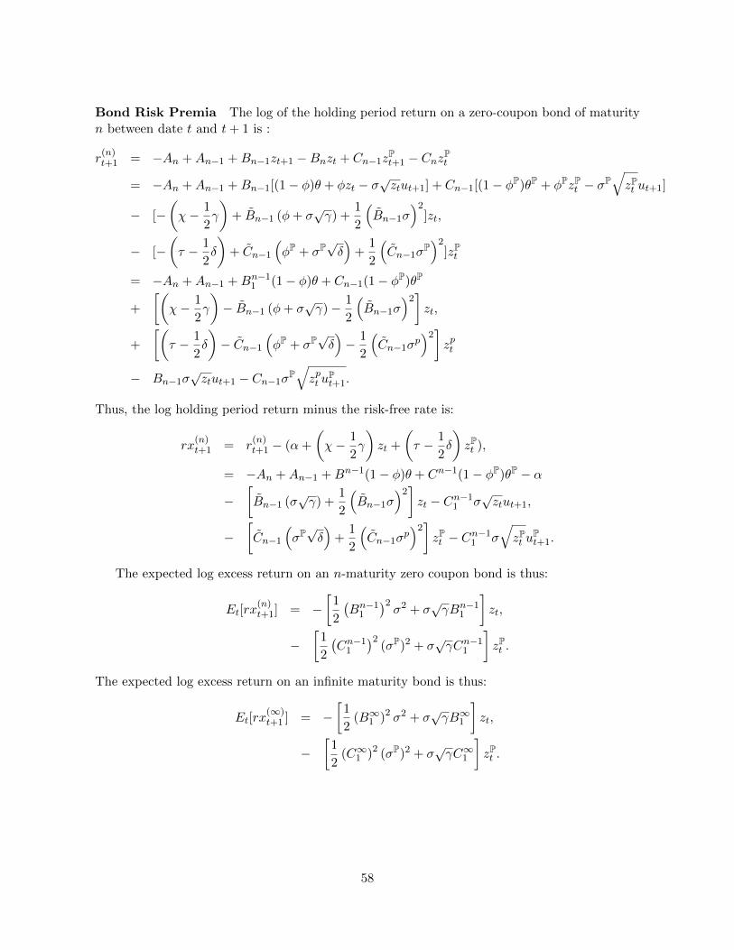
Bond Risk Premia The log of the holding period return on a zero-coupon bond of maturityn between date t and t+ 1 is :

r(n)t+1 = −An +An−1 +Bn−1zt+1 −Bnzt + Cn−1z

Pt+1 − CnzPt

= −An +An−1 +Bn−1[(1− φ)θ + φzt − σ√ztut+1] + Cn−1[(1− φP)θP + φPzPt − σP

√zPt ut+1]

− [−(χ− 1

2γ

)+ Bn−1 (φ+ σ

√γ) +

1

2

(Bn−1σ

)2]zt,

− [−(τ − 1

2δ

)+ Cn−1

(φP + σP

√δ)

+1

2

(Cn−1σ

P)2

]zPt

= −An +An−1 +Bn−11 (1− φ)θ + Cn−1(1− φP)θP

+

[(χ− 1

2γ

)− Bn−1 (φ+ σ

√γ)− 1

2

(Bn−1σ

)2]zt,

+

[(τ − 1

2δ

)− Cn−1

(φP + σP

√δ)− 1

2

(Cn−1σ

p)2]zpt

− Bn−1σ√ztut+1 − Cn−1σ

P√zpt u

Pt+1.

Thus, the log holding period return minus the risk-free rate is:

rx(n)t+1 = r

(n)t+1 − (α+

(χ− 1

2γ

)zt +

(τ − 1

2δ

)zPt ),

= −An +An−1 +Bn−1(1− φ)θ + Cn−1(1− φP)θP − α

−[Bn−1 (σ

√γ) +

1

2

(Bn−1σ

)2]zt − Cn−1

1 σ√ztut+1,

−[Cn−1

(σP√δ)

+1

2

(Cn−1σ

p)2]zPt − Cn−1

1 σ√zPt u

Pt+1.

The expected log excess return on an n-maturity zero coupon bond is thus:

Et[rx(n)t+1] = −

[1

2

(Bn−1

1

)2σ2 + σ

√γBn−1

1

]zt,

−[

1

2

(Cn−1

1

)2(σP)2 + σ

√γCn−1

1

]zPt .

The expected log excess return on an infinite maturity bond is thus:

Et[rx(∞)t+1 ] = −

[1

2(B∞1 )2 σ2 + σ

√γB∞1

]zt,

−[

1

2(C∞1 )2 (σP)2 + σ

√γC∞1

]zPt .

58

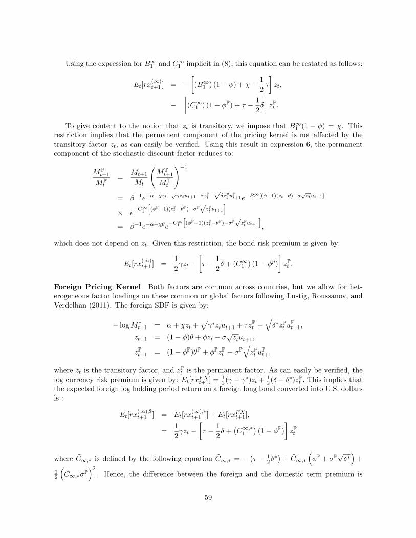
Using the expression for B∞1 and C∞1 implicit in (8), this equation can be restated as follows:

Et[rx(∞)t+1 ] = −

[(B∞1 ) (1− φ) + χ− 1

2γ

]zt,

−[(C∞1 ) (1− φP) + τ − 1

2δ

]zPt .

To give content to the notion that zt is transitory, we impose that B∞1 (1 − φ) = χ. Thisrestriction implies that the permanent component of the pricing kernel is not affected by thetransitory factor zt, as can easily be verified: Using this result in expression 6, the permanentcomponent of the stochastic discount factor reduces to:

MPt+1

MPt

=Mt+1

Mt

(MTt+1

MTt

)−1

= β−1e−α−χzt−√γztut+1−τzPt−

√δzpt u

Pt+1e−B

∞1 [(φ−1)(zt−θ)−σ

√ztut+1]

× e−C∞1

[(φP−1)(zPt−θP)−σP

√zPt ut+1

]= β−1e−α−χθe

−C∞1[(φP−1)(zPt−θP)−σP

√zPt ut+1

],

which does not depend on zt. Given this restriction, the bond risk premium is given by:

Et[rx(∞)t+1 ] =

1

2γzt −

[τ − 1

2δ + (C∞1 ) (1− φp)

]zPt .

Foreign Pricing Kernel Both factors are common across countries, but we allow for het-erogeneous factor loadings on these common or global factors following Lustig, Roussanov, andVerdelhan (2011). The foreign SDF is given by:

− logM∗t+1 = α+ χzt +√γ∗ztut+1 + τzPt +

√δ∗zPt u

Pt+1,

zt+1 = (1− φ)θ + φzt − σ√ztut+1,

zPt+1 = (1− φP)θP + φPzPt − σP√zPt u

Pt+1

where zt is the transitory factor, and zPt is the permanent factor. As can easily be verified, thelog currency risk premium is given by: Et[rx

FXt+1] = 1

2(γ − γ∗)zt + 12(δ− δ∗)zPt . This implies that

the expected foreign log holding period return on a foreign long bond converted into U.S. dollarsis :

Et[rx(∞),$t+1 ] = Et[rx

(∞),∗t+1 ] + Et[rx

FXt+1],

=1

2γzt −

[τ − 1

2δ +

(C∞,∗1

)(1− φP)

]zPt

where C∞,∗ is defined by the following equation C∞,∗ = −(τ − 1

2δ∗) + C∞,∗

(φP + σP

√δ∗)

+

12

(C∞,∗σ

P)2

. Hence, the difference between the foreign and the domestic term premium is

59

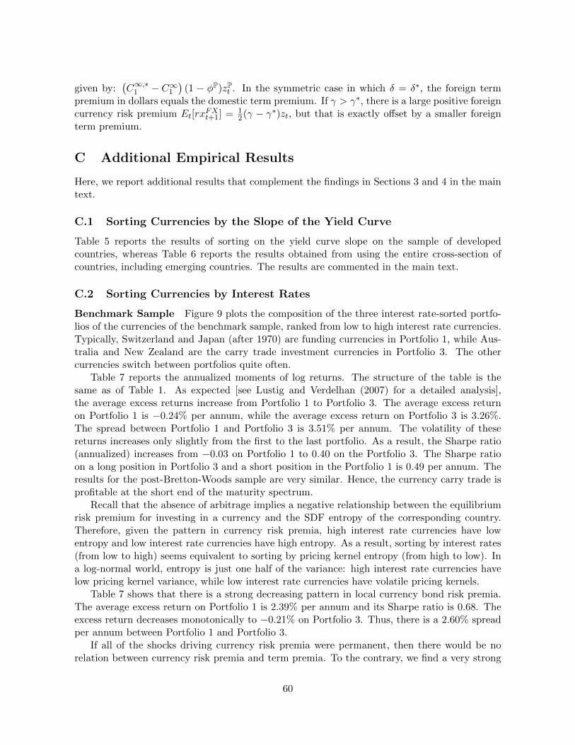
given by:(C∞,∗1 − C∞1

)(1 − φP)zPt . In the symmetric case in which δ = δ∗, the foreign term

premium in dollars equals the domestic term premium. If γ > γ∗, there is a large positive foreigncurrency risk premium Et[rx

FXt+1] = 1

2(γ − γ∗)zt, but that is exactly offset by a smaller foreignterm premium.

C Additional Empirical Results

Here, we report additional results that complement the findings in Sections 3 and 4 in the maintext.

C.1 Sorting Currencies by the Slope of the Yield Curve

Table 5 reports the results of sorting on the yield curve slope on the sample of developedcountries, whereas Table 6 reports the results obtained from using the entire cross-section ofcountries, including emerging countries. The results are commented in the main text.

C.2 Sorting Currencies by Interest Rates

Benchmark Sample Figure 9 plots the composition of the three interest rate-sorted portfo-lios of the currencies of the benchmark sample, ranked from low to high interest rate currencies.Typically, Switzerland and Japan (after 1970) are funding currencies in Portfolio 1, while Aus-tralia and New Zealand are the carry trade investment currencies in Portfolio 3. The othercurrencies switch between portfolios quite often.

Table 7 reports the annualized moments of log returns. The structure of the table is thesame as of Table 1. As expected [see Lustig and Verdelhan (2007) for a detailed analysis],the average excess returns increase from Portfolio 1 to Portfolio 3. The average excess returnon Portfolio 1 is −0.24% per annum, while the average excess return on Portfolio 3 is 3.26%.The spread between Portfolio 1 and Portfolio 3 is 3.51% per annum. The volatility of thesereturns increases only slightly from the first to the last portfolio. As a result, the Sharpe ratio(annualized) increases from −0.03 on Portfolio 1 to 0.40 on the Portfolio 3. The Sharpe ratioon a long position in Portfolio 3 and a short position in the Portfolio 1 is 0.49 per annum. Theresults for the post-Bretton-Woods sample are very similar. Hence, the currency carry trade isprofitable at the short end of the maturity spectrum.

Recall that the absence of arbitrage implies a negative relationship between the equilibriumrisk premium for investing in a currency and the SDF entropy of the corresponding country.Therefore, given the pattern in currency risk premia, high interest rate currencies have lowentropy and low interest rate currencies have high entropy. As a result, sorting by interest rates(from low to high) seems equivalent to sorting by pricing kernel entropy (from high to low). Ina log-normal world, entropy is just one half of the variance: high interest rate currencies havelow pricing kernel variance, while low interest rate currencies have volatile pricing kernels.

Table 7 shows that there is a strong decreasing pattern in local currency bond risk premia.The average excess return on Portfolio 1 is 2.39% per annum and its Sharpe ratio is 0.68. Theexcess return decreases monotonically to −0.21% on Portfolio 3. Thus, there is a 2.60% spreadper annum between Portfolio 1 and Portfolio 3.

If all of the shocks driving currency risk premia were permanent, then there would be norelation between currency risk premia and term premia. To the contrary, we find a very strong

60

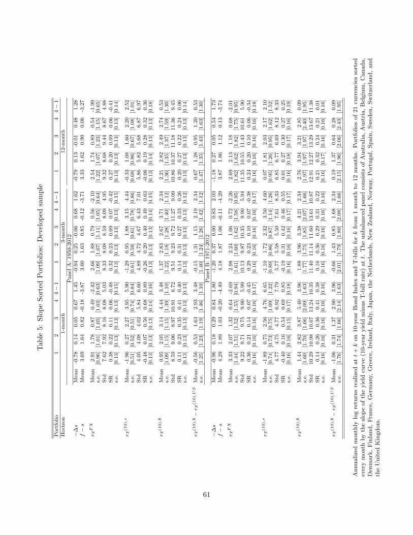
Tab

le5:

Slo

pe

Sor

ted

Por

tfol

ios:

Dev

elop

edsa

mp

le

Port

folio

12

34

4−

11

23

44−

11

23

44−

1H

ori

zon

1-m

onth

3-m

onth

12-m

onth

Pan

elA

:1950-2

012

−∆s

Mea

n-0

.78

0.1

40.0

50.6

71.4

5-0

.94

0.2

5-0

.06

0.6

81.6

2-0

.79

0.1

3-0

.01

0.4

81.2

8f−s

Mea

n3.6

91.6

40.8

2-0

.18

-3.8

73.6

01.6

30.8

5-0

.12

-3.7

13.3

31.6

20.9

00.0

6-3

.27

rxFX

Mea

n2.9

11.7

80.8

70.4

9-2

.42

2.6

61.8

80.7

90.5

6-2

.10

2.5

41.7

40.8

90.5

4-1

.99

s.e.

[0.9

6]

[1.0

1]

[1.0

5]

[1.0

3]

[0.6

3]

[1.0

9]

[1.0

7]

[1.1

1]

[1.0

5]

[0.6

4]

[1.2

2]

[1.0

7]

[1.2

3]

[1.1

5]

[0.6

5]

Std

7.6

27.9

28.1

68.0

85.0

38.3

38.0

88.5

98.0

94.9

59.3

28.6

89.4

48.6

74.8

8S

R0.3

80.2

20.1

10.0

6-0

.48

0.3

20.2

30.0

90.0

7-0

.42

0.2

70.2

00.0

90.0

6-0

.41

s.e.

[0.1

3]

[0.1

3]

[0.1

3]

[0.1

3]

[0.1

5]

[0.1

3]

[0.1

3]

[0.1

3]

[0.1

3]

[0.1

5]

[0.1

3]

[0.1

3]

[0.1

3]

[0.1

3]

[0.1

4]

rx(1

0),∗

Mea

n-1

.96

0.2

72.2

73.9

55.9

0-1

.29

0.9

51.8

83.1

54.4

4-0

.33

1.0

81.6

02.2

02.5

2s.

e.[0

.51]

[0.5

2]

[0.5

1]

[0.7

4]

[0.8

4]

[0.6

1]

[0.5

8]

[0.6

1]

[0.7

8]

[0.8

6]

[0.6

8]

[0.8

6]

[0.6

7]

[1.0

8]

[1.0

1]

Std

4.0

54.0

84.0

25.8

46.6

04.8

94.7

24.6

76.4

37.0

15.8

65.8

25.6

86.8

76.9

7S

R-0

.48

0.0

70.5

60.6

80.8

9-0

.26

0.2

00.4

00.4

90.6

3-0

.06

0.1

90.2

80.3

20.3

6s.

e.[0

.13]

[0.1

3]

[0.1

3]

[0.1

4]

[0.1

6]

[0.1

3]

[0.1

3]

[0.1

3]

[0.1

4]

[0.1

5]

[0.1

3]

[0.1

4]

[0.1

3]

[0.1

3]

[0.1

8]

rx(1

0),$

Mea

n0.9

52.0

53.1

44.4

43.4

81.3

72.8

32.6

73.7

12.3

42.2

12.8

22.4

92.7

40.5

3s.

e.[1

.09]

[1.1

5]

[1.1

5]

[1.3

9]

[1.1

0]

[1.2

2]

[1.1

8]

[1.2

8]

[1.4

0]

[1.1

2]

[1.3

6]

[1.3

5]

[1.3

7]

[1.5

9]

[1.3

0]

Std

8.5

99.0

68.9

710.9

18.7

29.5

19.2

39.7

211.2

79.0

910.8

610.3

711.1

811.3

69.4

5S

R0.1

10.2

30.3

50.4

10.4

00.1

40.3

10.2

70.3

30.2

60.2

00.2

70.2

20.2

40.0

6s.

e.[0

.13]

[0.1

3]

[0.1

3]

[0.1

3]

[0.1

3]

[0.1

3]

[0.1

3]

[0.1

3]

[0.1

3]

[0.1

2]

[0.1

3]

[0.1

3]

[0.1

3]

[0.1

3]

[0.1

4]

rx(1

0),$−rx(1

0),US

Mea

n-0

.56

0.5

31.6

32.9

33.4

8-0

.15

1.3

11.1

52.1

92.3

40.6

71.2

80.9

51.2

00.5

3s.

e.[1

.25]

[1.2

3]

[1.1

9]

[1.4

6]

[1.1

0]

[1.4

0]

[1.2

4]

[1.2

6]

[1.4

2]

[1.1

2]

[1.4

7]

[1.3

5]

[1.4

3]

[1.6

3]

[1.3

0]

Pan

elB

:1971-2

012

−∆s

Mea

n-0

.96

0.1

80.2

90.8

41.8

0-1

.20

0.3

70.0

00.8

32.0

3-1

.18

0.2

70.0

50.5

41.7

3f−s

Mea

n4.2

91.8

91.0

3-0

.20

-4.4

94.1

81.8

71.0

6-0

.11

-4.2

93.8

71.8

61.1

20.1

3-3

.74

rxFX

Mea

n3.3

32.0

71.3

20.6

4-2

.69

2.9

82.2

41.0

60.7

2-2

.26

2.6

92.1

31.1

80.6

8-2

.01

s.e.

[1.4

4]

[1.5

1]

[1.5

2]

[1.5

5]

[0.9

4]

[1.6

1]

[1.6

0]

[1.6

2]

[1.5

8]

[0.9

5]

[1.8

2]

[1.6

2]

[1.8

2]

[1.7

5]

[0.9

5]

Std

9.2

29.7

19.7

59.9

05.9

910.1

39.8

710.3

59.9

05.9

411.3

510.5

511.4

310.6

15.9

0S

R0.3

60.2

10.1

40.0

7-0

.45

0.2

90.2

30.1

00.0

7-0

.38

0.2

40.2

00.1

00.0

6-0

.34

s.e.

[0.1

6]

[0.1

6]

[0.1

6]

[0.1

6]

[0.1

7]

[0.1

6]

[0.1

6]

[0.1

6]

[0.1

6]

[0.1

7]

[0.1

6]

[0.1

6]

[0.1

6]

[0.1

6]

[0.1

8]

rx(1

0),∗

Mea

n-1

.89

0.7

52.5

64.7

66.6

5-1

.10

1.7

22.3

23.5

04.6

00.0

71.8

12.0

32.1

72.1

0s.

e.[0

.74]

[0.7

3]

[0.7

5]

[1.0

9]

[1.2

2]

[0.8

9]

[0.8

6]

[0.8

7]

[1.1

4]

[1.2

6]

[0.9

5]

[1.2

6]

[0.9

5]

[1.6

2]

[1.5

2]

Std

4.7

74.7

54.7

76.9

27.7

95.7

75.5

85.5

07.6

18.3

36.8

56.7

76.6

98.1

28.3

3S

R-0

.40

0.1

60.5

40.6

90.8

5-0

.19

0.3

10.4

20.4

60.5

50.0

10.2

70.3

00.2

70.2

5s.

e.[0

.16]

[0.1

6]

[0.1

5]

[0.1

7]

[0.1

8]

[0.1

6]

[0.1

6]

[0.1

6]

[0.1

7]

[0.1

7]

[0.1

6]

[0.1

8]

[0.1

7]

[0.1

6]

[0.1

9]

rx(1

0),$

Mea

n1.4

42.8

23.8

75.4

03.9

61.8

83.9

63.3

84.2

12.3

42.7

63.9

43.2

12.8

50.0

9s.

e.[1

.60]

[1.7

0]

[1.6

6]

[2.0

9]

[1.6

3]

[1.7

7]

[1.7

5]

[1.8

5]

[2.0

7]

[1.6

6]

[1.9

7]

[1.9

7]

[1.9

7]

[2.4

0]

[1.9

5]

Std

10.2

910.9

810.6

713.2

410.3

511.4

011.1

411.6

013.6

110.8

712.9

112.2

713.2

913.6

711.3

8S

R0.1

40.2

60.3

60.4

10.3

80.1

60.3

60.2

90.3

10.2

20.2

10.3

20.2

40.2

10.0

1s.

e.[0

.16]

[0.1

6]

[0.1

6]

[0.1

6]

[0.1

6]

[0.1

6]

[0.1

6]

[0.1

6]

[0.1

6]

[0.1

6]

[0.1

6]

[0.1

7]

[0.1

6]

[0.1

6]

[0.1

6]

rx(1

0),$−rx(1

0),US

Mea

n-1

.06

0.3

11.3

72.9

03.9

6-0

.66

1.4

30.8

51.6

82.3

40.1

91.3

70.6

40.2

80.0

9s.

e.[1

.76]

[1.7

4]

[1.6

6]

[2.1

4]

[1.6

3]

[2.0

1]

[1.7

9]

[1.8

0]

[2.0

8]

[1.6

6]

[2.1

5]

[1.9

6]

[2.0

6]

[2.4

3]

[1.9

5]

Annualize

dm

onth

lylo

gre

turn

sre

alize

datt

+k

on

10-y

ear

Bond

Index

and

T-b

ills

fork

from

1m

onth

to12

month

s.P

ort

folios

of

21

curr

enci

esso

rted

ever

ym

onth

by

the

slop

eof

the

yie

ldcu

rve

(10-y

ear

yie

ldm

inus

T-b

ill

rate

)att.

The

unbala

nce

dpanel

consi

sts

of

Aust

ralia,

Aust

ria,

Bel

giu

m,

Canada,

Den

mark

,F

inla

nd,

Fra

nce

,G

erm

any,

Gre

ece,

Irel

and,

Italy

,Japan,

the

Net

her

lands,

New

Zea

land,

Norw

ay,

Port

ugal,

Spain

,Sw

eden

,Sw

itze

rland,

and

the

Unit

edK

ingdom

.

61

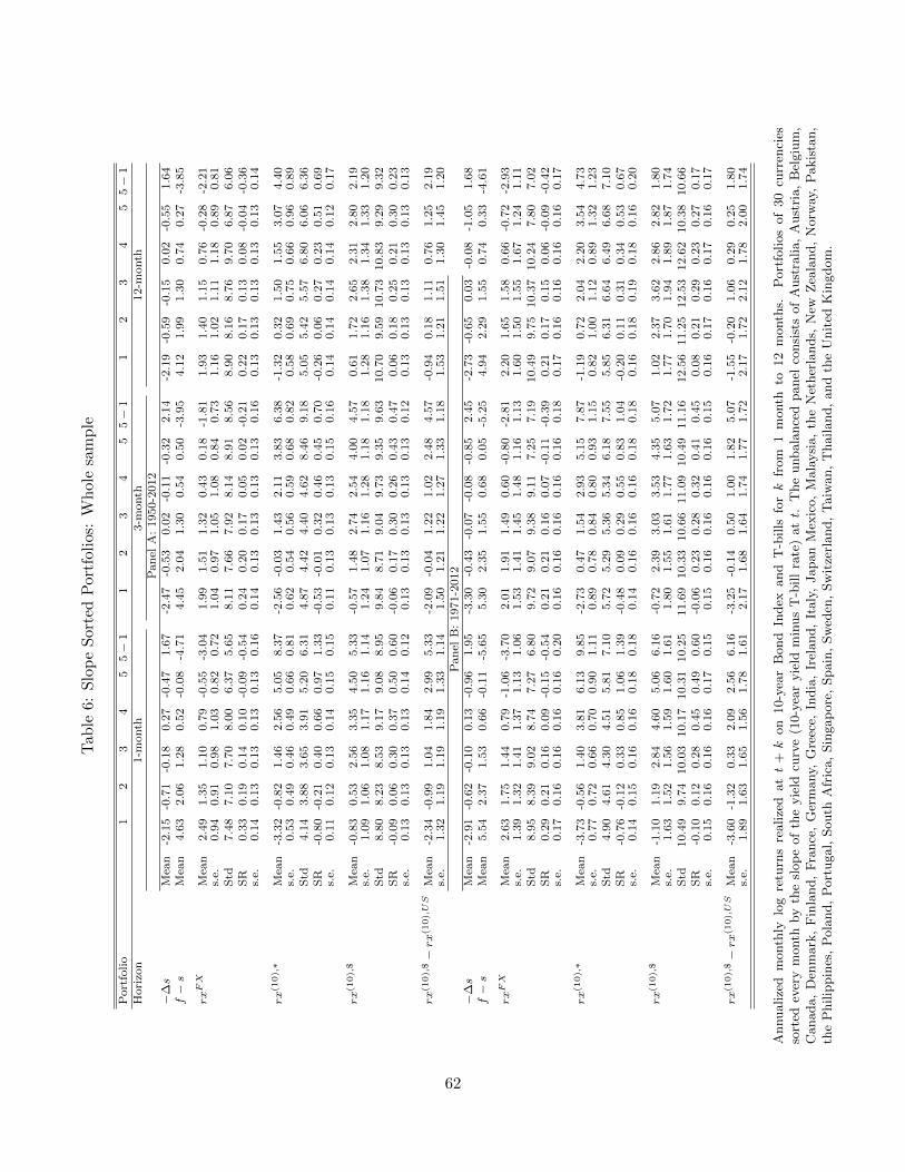
Tab

le6:

Slo

pe

Sor

ted

Por

tfol

ios:

Wh

ole

sam

ple

Port

folio

12

34

55−

11

23

45

5−

11

23

45

5−

1H

ori

zon

1-m

onth

3-m

onth

12-m

onth

Pan

elA

:1950-2

012

−∆s

Mea

n-2

.15

-0.7

1-0

.18

0.2

7-0

.47

1.6

7-2

.47

-0.5

30.0

2-0

.11

-0.3

22.1

4-2

.19

-0.5

9-0

.15

0.0

2-0

.55

1.6

4f−s

Mea

n4.6

32.0

61.2

80.5

2-0

.08

-4.7

14.4

52.0

41.3

00.5

40.5

0-3

.95

4.1

21.9

91.3

00.7

40.2

7-3

.85

rxFX

Mea

n2.4

91.3

51.1

00.7

9-0

.55

-3.0

41.9

91.5

11.3

20.4

30.1

8-1

.81

1.9

31.4

01.1

50.7

6-0

.28

-2.2

1s.

e.0.9

40.9

10.9

81.0

30.8

20.7

21.0

40.9

71.0

51.0

80.8

40.7

31.1

61.0

21.1

11.1

80.8

90.8

1S

td7.4

87.1

07.7

08.0

06.3

75.6

58.1

17.6

67.9

28.1

48.9

18.5

68.9

08.1

68.7

69.7

06.8

76.0

6S

R0.3

30.1

90.1

40.1

0-0

.09

-0.5

40.2

40.2

00.1

70.0

50.0

2-0

.21

0.2

20.1

70.1

30.0

8-0

.04

-0.3

6s.

e.0.1

40.1

30.1

30.1

30.1

30.1

60.1

40.1

30.1

30.1

30.1

30.1

60.1

30.1

30.1

30.1

30.1

30.1

4

rx(1

0),∗

Mea

n-3

.32

-0.8

21.4

62.5

65.0

58.3

7-2

.56

-0.0

31.4

32.1

13.8

36.3

8-1

.32

0.3

21.5

01.5

53.0

74.4

0s.

e.0.5

30.4

90.4

60.4

90.6

60.8

10.6

20.5

40.5

60.5

90.6

80.8

20.5

80.6

90.7

50.6

60.9

60.8

9S

td4.1

43.8

83.6

53.9

15.2

06.3

14.8

74.4

24.4

04.6

28.4

69.1

85.0

55.4

25.5

76.8

06.0

66.3

6S

R-0

.80

-0.2

10.4

00.6

60.9

71.3

3-0

.53

-0.0

10.3

20.4

60.4

50.7

0-0

.26

0.0

60.2

70.2

30.5

10.6

9s.

e.0.1

10.1

20.1

30.1

40.1

50.1

50.1

10.1

30.1

30.1

30.1

50.1

60.1

40.1

40.1

40.1

40.1

20.1

7

rx(1

0),$

Mea

n-0

.83

0.5

32.5

63.3

54.5

05.3

3-0

.57

1.4

82.7

42.5

44.0

04.5

70.6

11.7

22.6

52.3

12.8

02.1

9s.

e.1.0

91.0

61.0

81.1

71.1

61.1

41.2

41.0

71.1

61.2

81.1

81.1

81.2

81.1

61.3

81.3

41.3

31.2

0S

td8.8

08.2

38.5

39.1

79.0

88.9

59.8

48.7

19.0

49.7

39.3

59.6

310.7

09.5

910.7

310.8

39.2

99.3

2S

R-0

.09

0.0

60.3

00.3

70.5

00.6

0-0

.06

0.1

70.3

00.2

60.4

30.4

70.0

60.1

80.2

50.2

10.3

00.2

3s.

e.0.1

30.1

30.1

30.1

30.1

40.1

20.1

30.1

30.1

30.1

30.1

30.1

20.1

30.1

30.1

30.1

30.1

30.1

3

rx(1

0),$−rx(1

0),US

Mea

n-2

.34

-0.9

91.0

41.8

42.9

95.3

3-2

.09

-0.0

41.2

21.0

22.4

84.5

7-0

.94

0.1

81.1

10.7

61.2

52.1

9s.

e.1.3

21.1

91.1

91.1

91.3

31.1

41.5

01.2

11.2

21.2

71.3

31.1

81.5

31.2

11.5

11.3

01.4

51.2

0P

an

elB

:1971-2

012

−∆s

Mea

n-2

.91

-0.6

2-0

.10

0.1

3-0

.96

1.9

5-3

.30

-0.4

3-0

.07

-0.0

8-0

.85

2.4

5-2

.73

-0.6

50.0

3-0

.08

-1.0

51.6

8f−s

Mea

n5.5

42.3

71.5

30.6

6-0

.11

-5.6

55.3

02.3

51.5

50.6

80.0

5-5

.25

4.9

42.2

91.5

50.7

40.3

3-4

.61

rxFX

Mea

n2.6

31.7

51.4

40.7

9-1

.06

-3.7

02.0

11.9

11.4

90.6

0-0

.80

-2.8

12.2

01.6

51.5

80.6

6-0

.72

-2.9

3s.

e.1.3

91.3

21.4

11.3

71.1

31.0

61.5

31.4

11.4

51.4

81.1

61.1

31.6

01.5

01.5

51.6

71.2

41.1

1S

td8.9

58.3

99.0

28.7

47.2

76.8

09.7

29.0

79.3

89.1

17.2

57.1

910.4

99.7

510.3

710.2

47.8

07.0

2S

R0.2

90.2

10.1

60.0

9-0

.15

-0.5

40.2

10.2

10.1

60.0

7-0

.11

-0.3

90.2

10.1

70.1

50.0

6-0

.09

-0.4

2s.

e.0.1

70.1

60.1

60.1

60.1

60.2

00.1

60.1

60.1

60.1

60.1

60.1

80.1

70.1

60.1

60.1

60.1

60.1

7

rx(1

0),∗

Mea

n-3

.73

-0.5

61.4

03.8

16.1

39.8

5-2

.73

0.4

71.5

42.9

35.1

57.8

7-1

.19

0.7

22.0

42.2

03.5

44.7

3s.

e.0.7

70.7

20.6

60.7

00.9

01.1

10.8

90.7

80.8

40.8

00.9

31.1

50.8

21.0

01.1

20.8

91.3

21.2

3S

td4.9

04.6

14.3

04.5

15.8

17.1

05.7

25.2

95.3

65.3

46.1

87.5

55.8

56.3

16.6

46.4

96.6

87.1

0S

R-0

.76

-0.1

20.3

30.8

51.0

61.3

9-0

.48

0.0

90.2

90.5

50.8

31.0

4-0

.20

0.1

10.3

10.3

40.5

30.6

7s.

e.0.1

40.1

50.1

60.1

60.1

80.1

80.1

40.1

60.1

60.1

60.1

80.1

80.1

60.1

80.1

90.1

80.1

60.2

0

rx(1

0),$

Mea

n-1

.10

1.1

92.8

44.6

05.0

66.1

6-0

.72

2.3

93.0

33.5

34.3

55.0

71.0

22.3

73.6

22.8

62.8

21.8

0s.

e.1.6

31.5

21.5

61.5

91.6

01.6

11.8

01.5

51.6

11.7

71.6

31.7

21.7

71.7

01.9

41.8

91.8

71.7

4S

td10.4

99.7

410.0

310.1

710.3

110.2

511.6

910.3

310.6

611.0

910.4

911.1

612.5

611.2

512.5

312.6

210.3

810.6

6S

R-0

.10

0.1

20.2

80.4

50.4

90.6

0-0

.06

0.2

30.2

80.3

20.4

10.4

50.0

80.2

10.2

90.2

30.2

70.1

7s.

e.0.1

50.1

60.1

60.1

60.1

70.1

50.1

50.1

60.1

60.1

60.1

60.1

50.1

60.1

70.1

60.1

70.1

60.1

7

rx(1

0),$−rx(1

0),US

Mea

n-3

.60

-1.3

20.3

32.0

92.5

66.1

6-3

.25

-0.1

40.5

01.0

01.8

25.0

7-1

.55

-0.2

01.0

60.2

90.2

51.8

0s.

e.1.8

91.6

31.6

51.5

61.7

81.6

12.1

71.6

81.6

41.7

41.7

71.7

22.1

71.7

22.1

21.7

82.0

01.7

4

Annualize

dm

onth

lylo

gre

turn

sre

alize

datt

+k

on

10-y

ear

Bond

Index

and

T-b

ills

fork

from

1m

onth

to12

month

s.P

ort

folios

of

30

curr

enci

esso

rted

ever

ym

onth

by

the

slop

eof

the

yie

ldcu

rve

(10-y

ear

yie

ldm

inus

T-b

ill

rate

)att.

The

unbala

nce

dpanel

consi

sts

of

Aust

ralia,

Aust

ria,

Bel

giu

m,

Canada,

Den

mark

,F

inla

nd,

Fra

nce

,G

erm

any,

Gre

ece,

India

,Ir

eland,

Italy

,Japan

Mex

ico,

Mala

ysi

a,

the

Net

her

lands,

New

Zea

land,

Norw

ay,

Pakis

tan,

the

Philip

pin

es,

Pola

nd,

Port

ugal,

South

Afr

ica,

Sin

gap

ore

,Spain

,Sw

eden

,Sw

itze

rland,

Taiw

an,

Thailand,

and

the

Unit

edK

ingdom

.

62

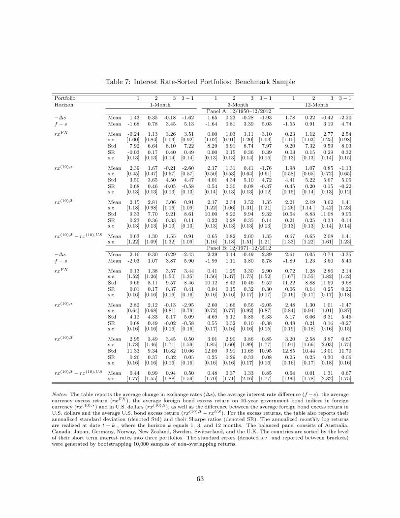
Table 7: Interest Rate-Sorted Portfolios: Benchmark Sample

Portfolio 1 2 3 3− 1 1 2 3 3− 1 1 2 3 3− 1

Horizon 1-Month 3-Month 12-MonthPanel A: 12/1950–12/2012

−∆s Mean 1.43 0.35 -0.18 -1.62 1.65 0.23 -0.28 -1.93 1.78 0.22 -0.42 -2.20f − s Mean -1.68 0.78 3.45 5.13 -1.64 0.81 3.39 5.03 -1.55 0.91 3.19 4.74

rxFX Mean -0.24 1.13 3.26 3.51 0.00 1.03 3.11 3.10 0.23 1.12 2.77 2.54s.e. [1.00] [0.84] [1.03] [0.92] [1.02] [0.91] [1.20] [1.03] [1.10] [1.03] [1.25] [0.98]Std 7.92 6.64 8.10 7.22 8.29 6.91 8.74 7.97 9.20 7.32 9.59 8.03SR -0.03 0.17 0.40 0.49 0.00 0.15 0.36 0.39 0.03 0.15 0.29 0.32s.e. [0.13] [0.13] [0.14] [0.14] [0.13] [0.13] [0.14] [0.15] [0.13] [0.13] [0.14] [0.15]

rx(10),∗ Mean 2.39 1.67 -0.21 -2.60 2.17 1.31 0.41 -1.76 1.98 1.07 0.85 -1.13s.e. [0.45] [0.47] [0.57] [0.57] [0.50] [0.53] [0.64] [0.61] [0.58] [0.65] [0.72] [0.65]Std 3.50 3.65 4.50 4.47 4.01 4.34 5.10 4.72 4.41 5.22 5.67 5.05SR 0.68 0.46 -0.05 -0.58 0.54 0.30 0.08 -0.37 0.45 0.20 0.15 -0.22s.e. [0.13] [0.13] [0.13] [0.13] [0.14] [0.13] [0.13] [0.12] [0.15] [0.14] [0.13] [0.12]

rx(10),$ Mean 2.15 2.81 3.06 0.91 2.17 2.34 3.52 1.35 2.21 2.19 3.62 1.41s.e. [1.18] [0.98] [1.16] [1.09] [1.22] [1.06] [1.31] [1.21] [1.26] [1.14 ] [1.42] [1.23]Std 9.33 7.70 9.21 8.61 10.00 8.22 9.94 9.32 10.64 8.83 11.08 9.95SR 0.23 0.36 0.33 0.11 0.22 0.28 0.35 0.14 0.21 0.25 0.33 0.14s.e. [0.13] [0.13] [0.13] [0.13] [0.13] [0.13] [0.13] [0.13] [0.13] [0.13] [0.14] [0.14]

rx(10),$ − rx(10),US Mean 0.63 1.30 1.55 0.91 0.65 0.82 2.00 1.35 0.67 0.65 2.08 1.41s.e. [1.22] [1.09] [1.32] [1.09] [1.16] [1.18] [1.51] [1.21] [1.33] [1.22] [1.61] [1.23]

Panel B: 12/1971–12/2012−∆s Mean 2.16 0.30 -0.29 -2.45 2.39 0.14 -0.49 -2.89 2.61 0.05 -0.74 -3.35f − s Mean -2.03 1.07 3.87 5.90 -1.99 1.11 3.80 5.78 -1.89 1.23 3.60 5.49

rxFX Mean 0.13 1.38 3.57 3.44 0.41 1.25 3.30 2.90 0.72 1.28 2.86 2.14s.e. [1.52] [1.26] [1.50] [1.35] [1.56] [1.37] [1.75] [1.52] [1.67] [1.55] [1.82] [1.42]Std 9.66 8.11 9.57 8.46 10.12 8.42 10.46 9.52 11.22 8.88 11.59 9.68SR 0.01 0.17 0.37 0.41 0.04 0.15 0.32 0.30 0.06 0.14 0.25 0.22s.e. [0.16] [0.16] [0.16] [0.16] [0.16] [0.16] [0.17] [0.17] [0.16] [0.17] [0.17] [0.18]

rx(10),∗ Mean 2.82 2.12 -0.13 -2.95 2.60 1.66 0.56 -2.05 2.48 1.30 1.01 -1.47s.e. [0.64] [0.68] [0.81] [0.79] [0.72] [0.77] [0.92] [0.87] [0.84] [0.94] [1.01] [0.87]Std 4.12 4.33 5.17 5.09 4.69 5.12 5.85 5.33 5.17 6.06 6.31 5.45SR 0.68 0.49 -0.02 -0.58 0.55 0.32 0.10 -0.38 0.48 0.21 0.16 -0.27s.e. [0.16] [0.16] [0.16] [0.16] [0.17] [0.16] [0.16] [0.15] [0.19] [0.18] [0.16] [0.15]


rx(10),$ − rx(10),US Mean 0.44 0.99 0.94 0.50 0.48 0.37 1.33 0.85 0.64 0.01 1.31 0.67s.e. [1.77] [1.55] [1.88] [1.59] [1.70] [1.71] [2.16] [1.77] [1.99] [1.78] [2.32] [1.75]

Notes: The table reports the average change in exchange rates (∆s), the average interest rate difference (f −s), the averagecurrency excess return (rxFX), the average foreign bond excess return on 10-year government bond indices in foreigncurrency (rx(10),∗) and in U.S. dollars (rx(10),$), as well as the difference between the average foreign bond excess return inU.S. dollars and the average U.S. bond excess return (rx(10),$ − rxUS). For the excess returns, the table also reports theirannualized standard deviation (denoted Std) and their Sharpe ratios (denoted SR). The annualized monthly log returnsare realized at date t + k , where the horizon k equals 1, 3, and 12 months. The balanced panel consists of Australia,Canada, Japan, Germany, Norway, New Zealand, Sweden, Switzerland, and the U.K. The countries are sorted by the levelof their short term interest rates into three portfolios. The standard errors (denoted s.e. and reported between brackets)were generated by bootstrapping 10,000 samples of non-overlapping returns.

63

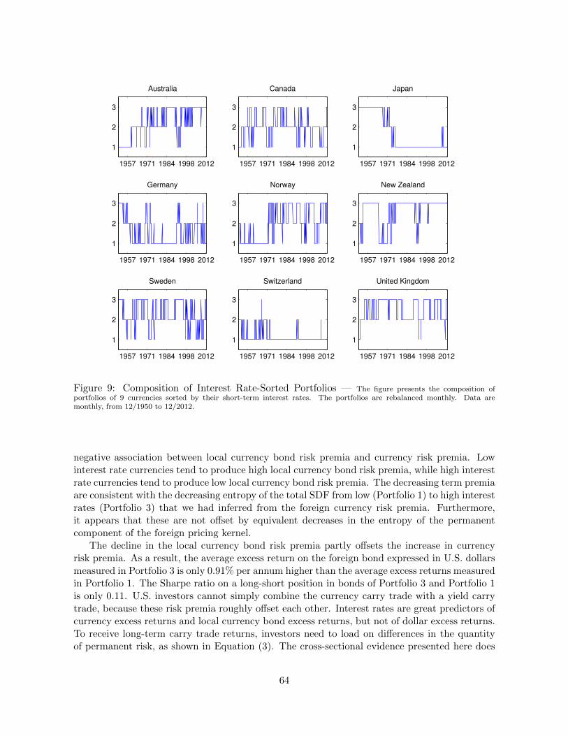
1957 1971 1984 1998 2012

1

2

3

Australia

1957 1971 1984 1998 2012

1

2

3

Canada

1957 1971 1984 1998 2012

1

2

3

Japan

1957 1971 1984 1998 2012

1

2

3

Germany

1957 1971 1984 1998 2012

1

2

3

Norway

1957 1971 1984 1998 2012

1

2

3

New Zealand

1957 1971 1984 1998 2012

1

2

3

Sweden

1957 1971 1984 1998 2012

1

2

3

Switzerland

1957 1971 1984 1998 2012

1

2

3

United Kingdom

Figure 9: Composition of Interest Rate-Sorted Portfolios — The figure presents the composition ofportfolios of 9 currencies sorted by their short-term interest rates. The portfolios are rebalanced monthly. Data aremonthly, from 12/1950 to 12/2012.

negative association between local currency bond risk premia and currency risk premia. Lowinterest rate currencies tend to produce high local currency bond risk premia, while high interestrate currencies tend to produce low local currency bond risk premia. The decreasing term premiaare consistent with the decreasing entropy of the total SDF from low (Portfolio 1) to high interestrates (Portfolio 3) that we had inferred from the foreign currency risk premia. Furthermore,it appears that these are not offset by equivalent decreases in the entropy of the permanentcomponent of the foreign pricing kernel.

The decline in the local currency bond risk premia partly offsets the increase in currencyrisk premia. As a result, the average excess return on the foreign bond expressed in U.S. dollarsmeasured in Portfolio 3 is only 0.91% per annum higher than the average excess returns measuredin Portfolio 1. The Sharpe ratio on a long-short position in bonds of Portfolio 3 and Portfolio 1is only 0.11. U.S. investors cannot simply combine the currency carry trade with a yield carrytrade, because these risk premia roughly offset each other. Interest rates are great predictors ofcurrency excess returns and local currency bond excess returns, but not of dollar excess returns.To receive long-term carry trade returns, investors need to load on differences in the quantityof permanent risk, as shown in Equation (3). The cross-sectional evidence presented here does

64

not lend much support to these differences in permanent risk.Table 7 shows that the results are essentially unchanged in the post-Bretton-Woods sample.

The Sharpe ratio on the currency carry trade is 0.41, achieved by going long in Portfolio 3 andshort in Portfolio 1. However, there is a strong decreasing pattern in local currency bond riskpremia, from 2.82% per annum in Portfolio 1 to −0.13% in the Portfolio 3. As a result, there isessentially no discernible pattern in dollar bond risk premia.

Figure 10 presents the cumulative one-month log returns on investments in foreign Treasurybills and foreign 10-year bonds. Most of the losses are concentrated in the 1970s and 1980s,and the bond returns do recover in the 1990s. In fact, between 1991 and 2012, the differenceis currency risk premia at the one-month horizon between Portfolio 1 and Portfolio 3 is 4.54%,while the difference in the local term premia is only 1.41% per annum. As a result, the un-hedgedcarry trade in 10-year bonds still earn about 3.13% per annum over this sample. However, thisdifference of 3.13% per annum has a standard error of 1.77% and, therefore, is not statisticallysignificant.

As we increase holding period k from 1 to 3 and 12 months, the differences in local bond riskpremia between portfolios shrink, but so do the differences in currency risk premia. Even at the12-month horizon, there is no evidence of statistically significant differences in dollar bond riskpremia across the currency portfolios.

Robustness Checks: Developed Countries and Whole Sample In the robustness tests,very similar patterns of risk premia emerge using larger sets of countries. In the sample ofdeveloped countries, we sort currencies in four portfolios. Figure 12 plots the composition ofthe four interest rate-sorted currency portfolios. Finally, Table 9 reports the results of sortingall the currencies in our sample, including those of emerging countries, into portfolios accordingto the level of their interest rate, ranked from low to high interest rate currencies. Switzerlandand Japan (after 1970) are funding currencies in Portfolio 1, while Australia and New Zealandare carry trade investment currencies in Portfolio 4. Credit risk seems to be concentrated inPortfolios 3 and 4.

Table 8 reports the results of sorting the developed country currencies into portfolios basedon the level of their interest rate, ranked from low to high interest rate currencies. Essentially,the results are very similar to those obtained on the benchmark sample of developed countries.There is no economically or statistically significant carry trade premium at longer maturities.The 2.98% spread in the currency risk premia is offset by the negative 3.03% spread in localterm premia at the one-month horizon against the carry trade currencies.

In the sample of developed and emerging countries, the pattern in returns is strikingly similar,but the differences are larger. At the one-month horizon, the 6.66% spread in the currency riskpremia is offset by a 5.15% spread in local term premia. A long-short position in foreign bondsdelivers an excess return of 1.51% per annum, which is not statistically significantly differentfrom zero. At longer horizons, the differences in local bond risk premia are much smaller, butso are the carry trade returns.

As in the previous samples, the rate at which the high interest rate currencies depreciate(2.99% per annum) is not high enough to offset the interest rate difference of 6.55%. Similarly,the rate at which the low interest rate currencies appreciate (0.43% per annum) is not highenough to offset the low interest rates (3.52% lower than the U.S. interest rate). Uncoveredinterest rate parity fails in the cross-section. However, the bond return differences (in local

65

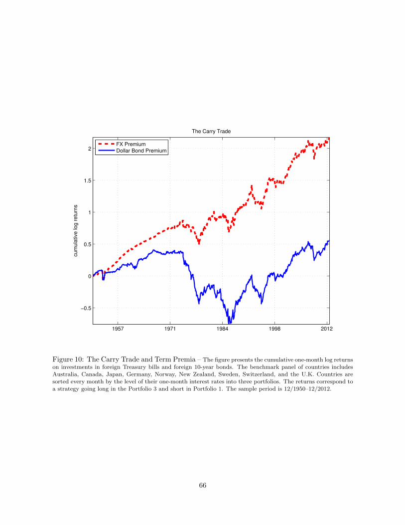
1957 1971 1984 1998 2012

−0.5

0

0.5

1

1.5

2

The Carry Trade

cum

ula

tive log r

etu

rns

FX Premium

Dollar Bond Premium

Figure 10: The Carry Trade and Term Premia – The figure presents the cumulative one-month log returnson investments in foreign Treasury bills and foreign 10-year bonds. The benchmark panel of countries includesAustralia, Canada, Japan, Germany, Norway, New Zealand, Sweden, Switzerland, and the U.K. Countries aresorted every month by the level of their one-month interest rates into three portfolios. The returns correspond toa strategy going long in the Portfolio 3 and short in Portfolio 1. The sample period is 12/1950–12/2012.

66

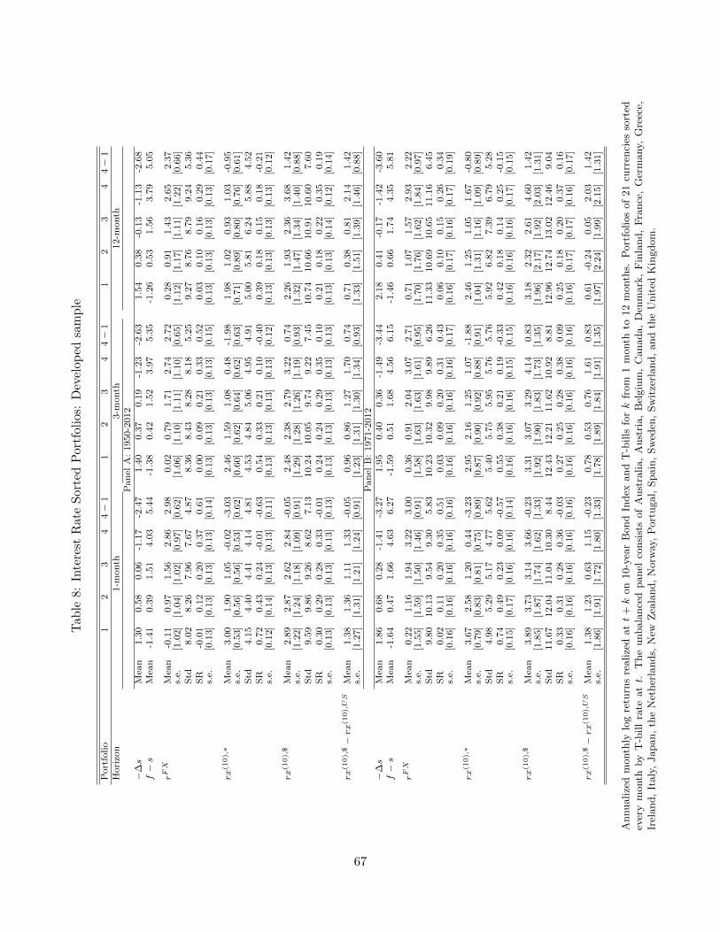
Tab

le8:

Inte

rest

Rat

eS

orte

dP

ortf

olio

s:D

evel

oped

sam

ple

Port

folio

12

34

4−

11

23

44−

11

23

44−

1H

ori

zon

1-m

onth

3-m

onth

12-m

onth

Pan

elA

:1950-2

012

−∆s

Mea

n1.3

00.5

80.0

6-1

.17

-2.4

71.4

00.3

70.1

9-1

.23

-2.6

31.5

40.3

8-0

.13

-1.1

3-2

.68

f−s

Mea

n-1

.41

0.3

91.5

14.0

35.4

4-1

.38

0.4

21.5

23.9

75.3

5-1

.26

0.5

31.5

63.7

95.0

5

rFX

Mea

n-0

.11

0.9

71.5

62.8

62.9

80.0

20.7

91.7

12.7

42.7

20.2

80.9

11.4

32.6

52.3

7s.

e.[1

.02]

[1.0

4]

[1.0

2]

[0.9

7]

[0.6

2]

[1.0

6]

[1.1

0]

[1.1

1]

[1.1

0]

[0.6

5]

[1.1

2]

[1.1

7]

[1.1

1]

[1.2

2]

[0.6

6]

Std

8.0

28.2

67.9

67.6

74.8

78.3

68.4

38.2

88.1

85.2

59.2

78.7

68.7

99.2

45.3

6S

R-0

.01

0.1

20.2

00.3

70.6

10.0

00.0

90.2

10.3

30.5

20.0

30.1

00.1

60.2

90.4

4s.

e.[0

.13]

[0.1

3]

[0.1

3]

[0.1

3]

[0.1

4]

[0.1

3]

[0.1

3]

[0.1

3]

[0.1

3]

[0.1

5]

[0.1

3]

[0.1

3]

[0.1

3]

[0.1

3]

[0.1

7]

rx(1

0),∗

Mea

n3.0

01.9

01.0

5-0

.02

-3.0

32.4

61.5

91.0

80.4

8-1

.98

1.9

81.0

20.9

31.0

3-0

.95

s.e.

[0.5

3]

[0.5

6]

[0.5

6]

[0.5

3]

[0.6

2]

[0.6

0]

[0.6

2]

[0.6

4]

[0.6

2]

[0.6

3]

[0.7

1]

[0.8

9]

[0.8

0]

[0.7

6]

[0.6

1]

Std

4.1

54.4

04.4

14.1

44.8

14.5

34.8

45.0

64.9

54.9

15.0

05.8

16.2

45.8

84.5

2S

R0.7

20.4

30.2

4-0

.01

-0.6

30.5

40.3

30.2

10.1

0-0

.40

0.3

90.1

80.1

50.1

8-0

.21

s.e.

[0.1

2]

[0.1

4]

[0.1

3]

[0.1

3]

[0.1

1]

[0.1

3]

[0.1

3]

[0.1

3]

[0.1

3]

[0.1

2]

[0.1

3]

[0.1

3]

[0.1

3]

[0.1

3]

[0.1

2]

rx(1

0),$

Mea

n2.8

92.8

72.6

22.8

4-0

.05

2.4

82.3

82.7

93.2

20.7

42.2

61.9

32.3

63.6

81.4

2s.

e.[1

.22]

[1.2

4]

[1.1

8]

[1.0

9]

[0.9

1]

[1.2

9]

[1.2

8]

[1.2

6]

[1.1

9]

[0.9

3]

[1.3

2]

[1.4

7]

[1.3

4]

[1.4

0]

[0.8

8]

Std

9.5

99.8

69.2

68.6

27.1

310.2

410.0

59.7

49.2

27.4

510.7

410.6

610.9

110.6

07.6

0S

R0.3

00.2

90.2

80.3

3-0

.01

0.2

40.2

40.2

90.3

50.1

00.2

10.1

80.2

20.3

50.1

9s.

e.[0

.13]

[0.1

3]

[0.1

3]

[0.1

3]

[0.1

3]

[0.1

3]

[0.1

3]

[0.1

3]

[0.1

3]

[0.1

3]

[0.1

3]

[0.1

3]

[0.1

4]

[0.1

2]

[0.1

4]

rx(1

0),$−rx(1

0),US

Mea

n1.3

81.3

61.1

11.3

3-0

.05

0.9

60.8

61.2

71.7

00.7

40.7

10.3

80.8

12.1

41.4

2s.

e.[1

.27]

[1.3

1]

[1.2

1]

[1.2

4]

[0.9

1]

[1.2

3]

[1.3

1]

[1.3

0]

[1.3

4]

[0.9

3]

[1.3

3]

[1.5

1]

[1.3

9]

[1.4

6]

[0.8

8]

Pan

elB

:1971-2

012

−∆s

Mea

n1.8

60.6

80.2

8-1

.41

-3.2

71.9

50.4

00.3

6-1

.49

-3.4

42.1

80.4

1-0

.17

-1.4

2-3

.60

f−s

Mea

n-1

.64

0.4

71.6

64.6

36.2

7-1

.59

0.5

11.6

84.5

66.1

5-1

.46

0.6

61.7

44.3

55.8

1

rFX

Mea

n0.2

21.1

61.9

43.2

23.0

00.3

60.9

12.0

43.0

72.7

10.7

11.0

71.5

72.9

32.2

2s.

e.[1

.55]

[1.5

9]

[1.5

0]

[1.4

6]

[0.9

1]

[1.5

8]

[1.6

3]

[1.6

3]

[1.6

1]

[0.9

5]

[1.7

0]

[1.7

6]

[1.6

2]

[1.8

4]

[0.9

7]

Std

9.8

010.1

39.5

49.3

05.8

310.2

310.3

29.9

89.8

96.2

611.3

310.6

910.6

511.1

66.4

5S

R0.0

20.1

10.2

00.3

50.5

10.0

30.0

90.2

00.3

10.4

30.0

60.1

00.1

50.2

60.3

4s.

e.[0

.16]

[0.1

6]

[0.1

6]

[0.1

6]

[0.1

6]

[0.1

6]

[0.1

6]

[0.1

6]

[0.1

6]

[0.1

7]

[0.1

6]

[0.1

7]

[0.1

6]

[0.1

7]

[0.1

9]

rx(1

0),∗

Mea

n3.6

72.5

81.2

00.4

4-3

.23

2.9

52.1

61.2

51.0

7-1

.88

2.4

61.2

51.0

51.6

7-0

.80

s.e.

[0.7

9]

[0.8

3]

[0.8

1]

[0.7

5]

[0.8

9]

[0.8

7]

[0.9

0]

[0.9

2]

[0.8

8]

[0.9

1]

[1.0

4]

[1.3

1]

[1.1

6]

[1.0

9]

[0.8

9]

Std

4.9

85.2

95.1

74.7

75.6

25.4

05.7

55.9

55.7

65.7

65.9

26.8

27.3

96.7

95.2

8S

R0.7

40.4

90.2

30.0

9-0

.57

0.5

50.3

80.2

10.1

9-0

.33

0.4

20.1

80.1

40.2

5-0

.15

s.e.

[0.1

5]

[0.1

7]

[0.1

6]

[0.1

6]

[0.1

4]

[0.1

6]

[0.1

6]

[0.1

6]

[0.1

5]

[0.1

5]

[0.1

6]

[0.1

6]

[0.1

6]

[0.1

7]

[0.1

5]

rx(1

0),$

Mea

n3.8

93.7

33.1

43.6

6-0

.23

3.3

13.0

73.2

94.1

40.8

33.1

82.3

22.6

14.6

01.4

2s.

e.[1

.85]

[1.8

7]

[1.7

4]

[1.6

2]

[1.3

3]

[1.9

2]

[1.9

0]

[1.8

3]

[1.7

3]

[1.3

5]

[1.9

6]

[2.1

7]

[1.9

2]

[2.0

3]

[1.3

1]

Std

11.6

712.0

411.0

410.3

08.4

412.4

312.2

111.6

210.9

28.8

112.9

612.7

413.0

212.4

69.0

4S

R0.3

30.3

10.2

80.3

6-0

.03

0.2

70.2

50.2

80.3

80.0

90.2

50.1

80.2

00.3

70.1

6s.

e.[0

.16]

[0.1

6]

[0.1

6]

[0.1

6]

[0.1

6]

[0.1

6]

[0.1

6]

[0.1

6]

[0.1

6]

[0.1

6]

[0.1

6]

[0.1

7]

[0.1

7]

[0.1

6]

[0.1

7]

rx(1

0),$−rx(1

0),US

Mea

n1.3

81.2

30.6

31.1

5-0

.23

0.7

80.5

30.7

61.6

10.8

30.6

1-0

.24

0.0

52.0

31.4

2s.

e.[1

.86]

[1.9

1]

[1.7

2]

[1.8

0]

[1.3

3]

[1.7

8]

[1.8

9]

[1.8

4]

[1.9

1]

[1.3

5]

[1.9

7]

[2.2

4]

[1.9

9]

[2.1

5]

[1.3

1]

Annualize

dm

onth

lylo

gre

turn

sre

alize

datt

+k

on

10-y

ear

Bond

Index

and

T-b

ills

fork

from

1m

onth

to12

month

s.P

ort

folios

of

21

curr

enci

esso

rted

ever

ym

onth

by

T-b

ill

rate

att.

The

unbala

nce

dpanel

consi

sts

of

Aust

ralia,

Aust

ria,

Bel

giu

m,

Canada,

Den

mark

,F

inla

nd,

Fra

nce

,G

erm

any,

Gre

ece,

Irel

and,

Italy

,Japan,

the

Net

her

lands,

New

Zea

land,

Norw

ay,

Port

ugal,

Spain

,Sw

eden

,Sw

itze

rland,

and

the

Unit

edK

ingdom

.

67

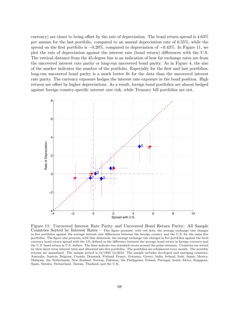
currency) are closer to being offset by the rate of depreciation. The bond return spread is 4.63%per annum for the last portfolio, compared to an annual depreciation rate of 6.55%, while thespread on the first portfolio is −0.29%, compared to depreciation of −0.43%. In Figure 11, weplot the rate of depreciation against the interest rate (bond return) differences with the U.S.The vertical distance from the 45-degree line is an indication of how far exchange rates are fromthe uncovered interest rate parity or long-run uncovered bond parity. As in Figure 4, the sizeof the marker indicates the number of the portfolio. Especially for the first and last portfolios,long-run uncovered bond parity is a much better fit for the data than the uncovered interestrate parity. The currency exposure hedges the interest rate exposure in the bond position. Highreturns are offset by higher depreciations. As a result, foreign bond portfolios are almost hedgedagainst foreign country-specific interest rate risk, while Treasury bill portfolios are not.

−4 −2 0 2 4 6 8 10−4

−2

0

2

4

6

8

12

3

4

5

12

3

4

5

Spread with U.S.

Rate

of D

epre

cia

tion

Figure 11: Uncovered Interest Rate Parity and Uncovered Bond Return Parity: All SampleCountries Sorted by Interest Rates – This figure presents, with red dots, the average exchange rate changesin five portfolios against the average interest rate differences between the foreign country and the U.S. for the same fiveportfolios. The figure also presents, with blue diamonds, the average exchange rate changes in five portfolios against the localcurrency bond return spread with the US, defined as the difference between the average bond return in foreign currency andthe U.S. bond return in U.S. dollars. The lines indicate two standard errors around the point estimate. Countries are sortedby their short-term interest rates and allocated into five portfolios. The portfolios are rebalanced every month. The monthlyreturns are annualized. The sample period is 12/1950–12/2012. The sample includes developed and emerging countries:Australia, Austria, Belgium, Canada, Denmark, Finland, France, Germany, Greece, India, Ireland, Italy, Japan, Mexico,Malaysia, the Netherlands, New Zealand, Norway, Pakistan, the Philippines, Poland, Portugal, South Africa, Singapore,Spain, Sweden, Switzerland, Taiwan, Thailand, and the U.K.

68

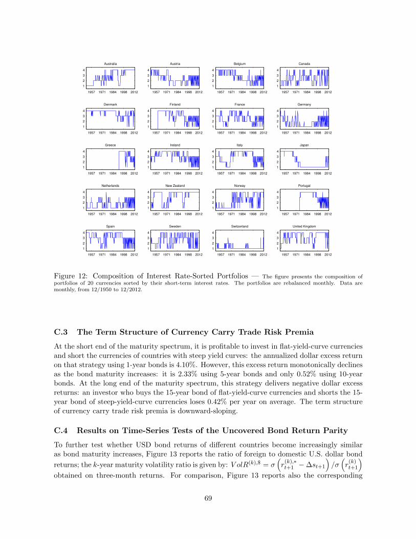
1957 1971 1984 1998 2012

1

2

3

4

Australia

1957 1971 1984 1998 2012

1

2

3

4

Austria

1957 1971 1984 1998 2012

1

2

3

4

Belgium

1957 1971 1984 1998 2012

1

2

3

4

Canada

1957 1971 1984 1998 2012

1

2

3

4

Denmark

1957 1971 1984 1998 2012

1

2

3

4

Finland

1957 1971 1984 1998 2012

1

2

3

4

France

1957 1971 1984 1998 2012

1

2

3

4

Germany

1957 1971 1984 1998 2012

1

2

3

4

Greece

1957 1971 1984 1998 2012

1

2

3

4

Ireland

1957 1971 1984 1998 2012

1

2

3

4

Italy

1957 1971 1984 1998 2012

1

2

3

4

Japan

1957 1971 1984 1998 2012

1

2

3

4

Netherlands

1957 1971 1984 1998 2012

1

2

3

4

New Zealand

1957 1971 1984 1998 2012

1

2

3

4

Norway

1957 1971 1984 1998 2012

1

2

3

4

Portugal

1957 1971 1984 1998 2012

1

2

3

4

Spain

1957 1971 1984 1998 2012

1

2

3

4

Sweden

1957 1971 1984 1998 2012

1

2

3

4

Switzerland

1957 1971 1984 1998 2012

1

2

3

4

United Kingdom

Figure 12: Composition of Interest Rate-Sorted Portfolios — The figure presents the composition ofportfolios of 20 currencies sorted by their short-term interest rates. The portfolios are rebalanced monthly. Data aremonthly, from 12/1950 to 12/2012.

C.3 The Term Structure of Currency Carry Trade Risk Premia

At the short end of the maturity spectrum, it is profitable to invest in flat-yield-curve currenciesand short the currencies of countries with steep yield curves: the annualized dollar excess returnon that strategy using 1-year bonds is 4.10%. However, this excess return monotonically declinesas the bond maturity increases: it is 2.33% using 5-year bonds and only 0.52% using 10-yearbonds. At the long end of the maturity spectrum, this strategy delivers negative dollar excessreturns: an investor who buys the 15-year bond of flat-yield-curve currencies and shorts the 15-year bond of steep-yield-curve currencies loses 0.42% per year on average. The term structureof currency carry trade risk premia is downward-sloping.

C.4 Results on Time-Series Tests of the Uncovered Bond Return Parity

To further test whether USD bond returns of different countries become increasingly similaras bond maturity increases, Figure 13 reports the ratio of foreign to domestic U.S. dollar bond

returns; the k-year maturity volatility ratio is given by: V olR(k),$ = σ(r

(k),∗t+1 −∆st+1

)/σ(r

(k)t+1

)obtained on three-month returns. For comparison, Figure 13 reports also the corresponding

69

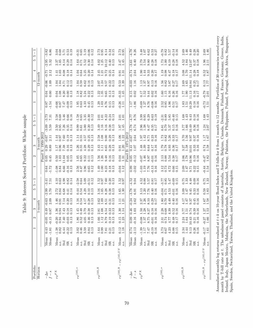
Tab

le9:

Inte

rest

Sor

ted

Por

tfol

ios:

Wh

ole

sam

ple

Port

folio

12

34

55−

11

23

45

5−

11

23

45

5−

1H

ori

zon

1-m

onth

3-m

onth

12-m

onth

Pan

elA

:1950-2

012

−∆s

Mea

n0.4

3-0

.05

0.4

9-0

.63

-2.9

9-3

.41

0.6

40.0

50.2

9-0

.67

-3.0

9-3

.73

0.8

70.0

4-0

.06

-0.7

1-2

.95

-3.8

2f−s

Mea

n-1

.81

-0.1

50.8

72.0

95.7

07.5

1-1

.72

0.4

50.8

92.1

15.5

97.3

1-1

.54

0.0

01.0

92.1

25.3

26.8

6

rxFX

Mea

n-1

.38

-0.2

01.3

61.4

62.7

24.1

0-1

.08

0.5

01.1

71.4

42.5

03.5

8-0

.66

0.0

41.0

41.4

12.3

73.0

4s.

e.0.8

20.9

40.9

40.9

10.8

40.6

30.8

41.0

30.9

60.9

70.9

50.6

80.8

71.0

81.0

41.0

31.0

50.6

8S

td6.4

47.4

07.4

37.1

46.6

84.9

86.6

611.0

47.3

87.6

07.2

65.4

67.4

78.2

08.7

18.0

88.1

45.7

1S

R-0

.22

-0.0

30.1

80.2

00.4

10.8

2-0

.16

0.0

50.1

60.1

90.3

50.6

6-0

.09

0.0

00.1

20.1

80.2

90.5

3s.

e.0.1

30.1

30.1

30.1

30.1

40.1

40.1

30.1

30.1

30.1

30.1

40.1

60.1

30.1

30.1

30.1

40.1

40.1

9

rx(1

0),∗

Mea

n3.0

21.8

61.4

51.1

60.4

4-2

.58

2.5

61.0

51.2

61.1

40.9

9-1

.58

1.9

51.1

81.0

41.0

41.6

4-0

.31

s.e.

0.4

60.5

20.4

80.5

40.5

40.6

40.4

70.6

50.5

50.5

50.6

10.6

50.6

30.8

20.5

90.6

40.7

10.6

5S

td3.5

94.0

53.7

94.1

74.2

95.0

93.9

69.2

24.2

84.5

75.0

05.3

54.3

35.2

46.6

25.2

55.5

25.1

9S

R0.8

40.4

60.3

80.2

80.1

0-0

.51

0.6

50.1

10.2

90.2

50.2

0-0

.30

0.4

50.2

20.1

60.2

00.3

0-0

.06

s.e.

0.1

30.1

30.1

30.1

30.1

30.1

20.1

20.1

30.1

30.1

30.1

30.1

20.1

30.1

30.1

30.1

40.1

40.1

2

rx(1

0),$

Mea

n1.6

41.6

62.8

12.6

23.1

61.5

21.4

91.5

62.4

32.5

83.4

92.0

11.2

91.2

22.0

72.4

54.0

22.7

3s.

e.0.9

91.1

21.0

81.0

91.0

50.9

71.0

01.2

61.1

11.0

81.1

61.0

11.0

31.3

51.2

41.2

11.2

50.9

5S

td7.8

18.7

98.5

48.5

18.2

87.6

08.2

39.4

88.6

59.0

09.1

68.2

28.7

69.6

59.5

79.7

210.1

28.1

4S

R0.2

10.1

90.3

30.3

10.3

80.2

00.1

80.1

60.2

80.2

90.3

80.2

40.1

50.1

30.2

20.2

50.4

00.3

4s.

e.0.1

30.1

30.1

30.1

30.1

30.1

30.1

30.1

30.1

30.1

30.1

30.1

30.1

30.1

30.1

30.1

40.1

30.1

5

rx(1

0),$−rx(1

0),US

Mea

n0.1

20.1

51.3

01.1

11.6

51.5

2-0

.04

0.0

40.9

11.0

61.9

72.0

1-0

.26

-0.3

30.5

30.9

12.4

72.7

3s.

e.1.1

81.2

31.1

41.2

11.3

00.9

71.1

21.3

11.2

01.2

21.4

51.0

11.1

11.4

51.3

91.3

11.4

50.9

5P

an

elB

:1971-2

012

−∆s

Mea

n0.7

40.0

90.4

6-0

.24

-3.7

8-4

.52

0.9

90.0

50.4

1-0

.67

-3.7

8-4

.77

1.1

70.1

5-0

.03

-0.7

4-3

.61

-4.7

8f−s

Mea

n-2

.13

-0.1

61.0

32.6

26.9

19.0

4-2

.02

-0.1

21.0

72.6

46.7

48.7

6-1

.86

0.0

21.1

62.6

46.4

08.2

6

rxFX

Mea

n-1

.39

-0.0

81.5

02.3

73.1

34.5

2-1

.03

-0.0

71.4

81.9

72.9

63.9

9-0

.69

0.1

71.1

31.9

02.7

93.4

8s.

e.1.1

71.3

71.2

81.2

61.2

00.8

81.1

91.4

61.3

91.4

21.3

80.9

51.2

71.5

21.3

71.4

41.5

41.0

7S

td7.4

78.7

58.2

78.1

07.7

65.5

77.7

68.9

78.6

48.7

18.4

76.2

98.7

69.4

48.9

79.3

39.8

06.6

2S

R-0

.19

-0.0

10.1

80.2

90.4

00.8

1-0

.13

-0.0

10.1

70.2

30.3

50.6

3-0

.08

0.0

20.1

30.2

00.2

80.5

3s.

e.0.1

60.1

60.1

60.1

70.1

60.1

70.1

60.1

60.1

60.1

60.1

70.1

90.1

60.1

60.1

60.1

70.1

80.2

7

rx(1

0),∗

Mea

n3.7

32.3

12.2

81.8

0-0

.04

-3.7

73.1

22.1

31.7

91.7

30.8

1-2

.31

2.5

21.6

01.5

61.1

91.7

3-0

.79

s.e.

0.6

70.7

40.6

80.7

00.7

10.8

50.7

30.8

80.7

80.8

20.7

90.8

90.8

51.1

50.8

20.9

81.0

00.8

2S

td4.2

34.7

74.3

94.4

94.5

35.4

74.7

25.5

44.9

35.2

65.3

75.8

54.9

66.1

65.8

76.4

76.1

95.5

7S

R0.8

80.4

80.5

20.4

0-0

.01

-0.6

90.6

60.3

80.3

60.3

30.1

5-0

.40

0.5

10.2

60.2

70.1

80.2

8-0

.14

s.e.

0.1

50.1

70.1

60.1

60.1

60.1

50.1

50.1

70.1

70.1

70.1

60.1

50.1

70.1

60.1

70.1

70.1

80.1

6

rx(1

0),$

Mea

n2.3

42.2

43.7

74.1

73.0

90.7

52.0

92.0

63.2

73.7

03.7

71.6

81.8

31.7

72.6

93.0

84.5

22.6

9s.

e.1.4

41.6

41.5

11.4

71.4

71.3

31.4

71.7

81.5

81.5

61.6

61.4

31.5

11.9

01.6

51.7

01.8

41.4

6S

td9.1

310.4

39.7

49.3

79.4

58.4

89.7

110.9

610.0

19.9

710.4

99.4

310.2

911.1

310.8

411.1

412.0

79.4

9S

R0.2

60.2

10.3

90.4

50.3

30.0

90.2

20.1

90.3

30.3

70.3

60.1

80.1

80.1

60.2

50.2

80.3

70.2

8s.

e.0.1

60.1

60.1

60.1

60.1

60.1

60.1

50.1

60.1

60.1

60.1

60.1

60.1

60.1

70.1

70.1

80.1

80.2

0

rx(1

0),$−rx(1

0),US

Mea

n-0

.17

-0.2

71.2

71.6

70.5

90.7

5-0

.44

-0.4

70.7

41.1

71.2

41.6

8-0

.73

-0.7

90.1

30.5

21.9

62.6

9s.

e.1.6

11.6

61.5

31.5

81.8

31.3

31.5

41.8

21.5

81.6

72.0

71.4

31.5

12.0

11.7

71.8

72.1

11.4

6

Annualize

dm

onth

lylo

gre

turn

sre

alize

datt+k

on

10-y

ear

Bond

Index

and

T-b

ills

fork

from

1m

onth

to12

month

s.P

ort

folios

of

30

curr

enci

esso

rted

ever

ym

onth

by

T-b

ill

rate

att.

The

unbala

nce

dpanel

consi

sts

of

Aust

ralia,

Aust

ria,

Bel

giu

m,

Canada,

Den

mark

,F

inla

nd,

Fra

nce

,G

erm

any,

Gre

ece,

India

,Ir

eland,

Italy

,Japan

Mex

ico,

Mala

ysi

a,

the

Net

her

lands,

New

Zea

land,

Norw

ay,

Pakis

tan,

the

Philip

pin

es,

Pola

nd,

Port

ugal,

South

Afr

ica,

Sin

gap

ore

,Spain

,Sw

eden

,Sw

itze

rland,

Taiw

an,

Thailand,

and

the

Unit

edK

ingdom

.

70

Tab

le10:

Th

eM

atu

rity

Str

uct

ure

ofR

etu

rns

inS

lop

e-S

orte

dP

ortf

olio

s:E

xte

nd

edS

am

ple

Matu

rity

4-q

uart

ers

20-q

uart

ers

40-q

uart

ers

60-q

uart

ers

Port

folio

12

34

55−

11

23

45

5−

11

23

45

5−

11

23

45

5−

1

−∆s

Mea

n0.9

00.5

90.2

92.3

4-0

.30

-1.1

90.9

00.5

90.2

92.3

4-0

.30

-1.1

90.9

00.5

90.2

92.3

4-0

.30

-1.1

90.9

40.4

30.3

52.3

8-0

.39

-1.3

3

f−s

Mea

n3.9

91.9

90.9

90.3

90.3

6-3

.63

3.9

91.9

90.9

90.3

90.3

6-3

.63

3.9

91.9

90.9

90.3

90.3

6-3

.63

3.9

32.0

00.9

50.3

20.3

2-3

.62

rxFX

Mea

n4.8

92.5

81.2

82.7

30.0

7-4

.82

4.8

92.5

81.2

82.7

30.0

7-4

.82

4.8

92.5

81.2

82.7

30.0

7-4

.82

4.8

72.4

31.3

02.7

0-0

.07

-4.9

4s.

e.[1

.26]

[1.1

8]

[1.1

9]

[1.1

6]

[0.9

8]

[0.9

1]

[1.2

6]

[1.1

9]

[1.1

9]

[1.1

7]

[0.9

8]

[0.9

0]

[1.2

6]

[1.1

8]

[1.2

0]

[1.1

6]

[0.9

8]

[0.9

1]

[1.2

6]

[1.1

8]

[1.1

9]

[1.1

9]

[0.9

9]

[0.9

1]

Std

11.0

010.3

610.4

410.2

48.5

67.9

511.0

010.3

610.4

410.2

48.5

67.9

511.0

010.3

610.4

410.2

48.5

67.9

511.0

110.3

410.4

410.4

48.6

57.9

9

SR

0.4

40.2

50.1

20.2

70.0

1-0

.61

0.4

40.2

50.1

20.2

70.0

1-0

.61

0.4

40.2

50.1

20.2

70.0

1-0

.61

0.4

40.2

40.1

20.2

6-0

.01

-0.6

2s.

e.[0

.13]

[0.1

2]

[0.1

2]

[0.1

2]

[0.1

2]

[0.1

2]

[0.1

2]

[0.1

2]

[0.1

2]

[0.1

2]

[0.1

2]

[0.1

2]

[0.1

2]

[0.1

2]

[0.1

2]

[0.1

2]

[0.1

1]

[0.1

2]

[0.1

2]

[0.1

2]

[0.1

2]

[0.1

2]

[0.1

2]

[0.1

2]

rx(k

),∗

Mea

n-0

.09

0.1

10.3

20.3

30.6

30.7

21.1

12.1

22.5

62.7

33.6

02.5

01.5

92.6

94.1

64.3

25.9

04.3

12.4

22.8

46.3

64.7

87.7

85.3

6s.

e.[0

.12]

[0.1

0]

[0.1

0]

[0.1

0]

[0.1

0]

[0.1

3]

[0.5

9]

[0.5

4]

[0.5

9]

[0.5

6]

[0.6

2]

[0.6

4]

[1.0

6]

[0.9

7]

[1.0

5]

[1.0

0]

[1.0

2]

[0.9

6]

[1.4

5]

[1.4

6]

[1.4

3]

[1.3

6]

[1.4

4]

[1.3

1]

Std

1.0

40.8

80.8

80.8

40.8

81.1

55.1

34.7

05.2

24.9

65.4

25.5

39.3

48.5

69.1

98.7

89.0

18.4

412.6

712.8

212.5

511.9

212.7

011.7

6

SR

-0.0

90.1

20.3

70.3

90.7

20.6

30.2

20.4

50.4

90.5

50.6

70.4

50.1

70.3

10.4

50.4

90.6

50.5

10.1

90.2

20.5

10.4

00.6

10.4

6s.

e.[0

.11]

[0.1

2]

[0.1

1]

[0.1

2]

[0.1

1]

[0.1

1]

[0.1

2]

[0.1

2]

[0.1

2]

[0.1

3]

[0.1

2]

[0.1

1]

[0.1

2]

[0.1

2]

[0.1

2]

[0.1

3]

[0.1

3]

[0.1

1]

[0.1

2]

[0.1

2]

[0.1

2]

[0.1

3]

[0.1

2]

[0.1

1]

rx(k

),$

Mea

n4.8

02.6

91.6

03.0

60.7

0-4

.10

6.0

04.7

03.8

45.4

63.6

7-2

.33

6.4

85.2

75.4

57.0

55.9

7-0

.52

7.2

95.2

77.6

67.4

77.7

10.4

2s.

e.[1

.26]

[1.1

7]

[1.1

7]

[1.1

6]

[1.0

0]

[0.9

1]

[1.3

5]

[1.2

6]

[1.2

3]

[1.3

0]

[1.2

2]

[1.0

5]

[1.5

9]

[1.4

8]

[1.5

0]

[1.5

5]

[1.4

8]

[1.2

6]

[1.8

7]

[1.8

4]

[1.7

8]

[1.8

2]

[1.8

0]

[1.5

4]

Std

11.0

510.2

910.3

210.2

78.7

27.9

911.8

711.0

711.0

211.5

010.7

19.1

714.1

013.1

313.2

513.8

413.1

411.2

416.4

516.1

015.7

416.0

415.9

613.9

7

SR

0.4

30.2

60.1

60.3

00.0

8-0

.51

0.5

10.4

20.3

50.4

70.3

4-0

.25

0.4

60.4

00.4

10.5

10.4

5-0

.05

0.4

40.3

30.4

90.4

70.4

80.0

3s.

e.[0

.12]

[0.1

2]

[0.1

2]

[0.1

2]

[0.1

2]

[0.1

2]

[0.1

2]

[0.1

2]

[0.1

2]

[0.1

2]

[0.1

2]

[0.1

2]

[0.1

2]

[0.1

2]

[0.1

2]

[0.1

2]

[0.1

2]

[0.1

2]

[0.1

2]

[0.1

2]

[0.1

2]

[0.1

2]

[0.1

2]

[0.1

2]

rx(k

),$−rx(k

),US

Mea

n7.6

65.5

64.4

75.9

23.5

7-4

.10

6.2

84.9

94.1

35.7

53.9

6-2

.33

4.8

93.6

83.8

65.4

64.3

8-0

.52

4.6

72.6

55.0

44.8

55.0

90.4

2s.

e.[1

.26]

[1.1

6]

[1.1

6]

[1.1

4]

[0.9

7]

[0.9

1]

[1.3

4]

[1.2

3]

[1.1

3]

[1.2

0]

[1.1

3]

[1.0

5]

[1.5

4]

[1.4

1]

[1.3

3]

[1.3

9]

[1.3

4]

[1.2

6]

[1.7

7]

[1.7

6]

[1.5

7]

[1.6

3]

[1.6

6]

[1.5

4]

Notes:

Th

eta

ble

rep

ort

ssu

mm

ary

stati

stic

son

an

nu

alize

dlo

gre

turn

sre

ali

zed

on

zero

cou

pon

bon

ds

wit

hm

atu

rity

vary

ing

fromk

=4

tok

=60

qu

art

ers.

Th

eh

old

ing

per

iod

ison

equ

art

er.

Th

eta

ble

rep

ort

sth

eaver

age

chan

ge

inex

chan

ge

rate

s(−

∆s)

,th

eaver

age

inte

rest

rate

diff

eren

ce(f−s)

,th

eaver

age

curr

ency

exce

ssre

turn

(rxFX

),th

eaver

age

fore

ign

bon

dex

cess

retu

rnin

fore

ign

curr

ency

(rx(k

),∗)

an

din

U.S

.d

ollars

(rx(k

),$),

as

wel

las

the

diff

eren

ceb

etw

een

the

aver

age

fore

ign

bon

dex

cess

retu

rnin

U.S

.d

ollars

an

dth

eaver

age

U.S

.b

on

dex

cess

retu

rn(rx(k

),$−rx(k

),US

).F

or

the

exce

ssre

turn

s,th

eta

ble

als

ore

port

sth

eir

an

nu

alize

dst

an

dard

dev

iati

on

(den

ote

dS

td)

an

dth

eir

Sh

arp

era

tios

(den

ote

dS

R).

Th

eu

nb

ala

nce

dp

an

elco

nsi

sts

of

Au

stra

lia,

Au

stri

a,

Bel

giu

m,

Can

ad

a,

the

Cze

chR

epu

blic,

Den

mark

,F

inla

nd

,F

ran

ce,

Ger

many,

Hu

ngary

,In

don

esia

,Ir

elan

d,

Italy

,Jap

an

,M

ala

ysi

a,

Mex

ico,

the

Net

her

lan

ds,

New

Zea

lan

d,

Norw

ay,

Pola

nd

,P

ort

ugal,

Sin

gap

ore

,S

ou

thA

fric

a,

Sp

ain

,S

wed

en,

Sw

itze

rlan

d,

an

dth

eU

.K.

Th

eco

untr

ies

are

sort

edby

the

slop

eof

thei

ryie

ldcu

rves

into

five

port

folios.

Th

esl

op

eof

the

yie

ldcu

rve

ism

easu

red

by

the

diff

eren

ceb

etw

een

the

10-y

ear

yie

ldan

dth

e3-m

onth

inte

rest

rate

at

datet.

Th

est

an

dard

erro

rs(d

enote

ds.

e.an

dre

port

edb

etw

een

bra

cket

s)w

ere

gen

erate

dby

boots

trap

pin

g10,0

00

sam

ple

sof

non

-over

lap

pin

gre

turn

s.D

ata

are

qu

art

erly

an

dth

esa

mp

lew

ind

ow

is5/1987–12/2012.

71

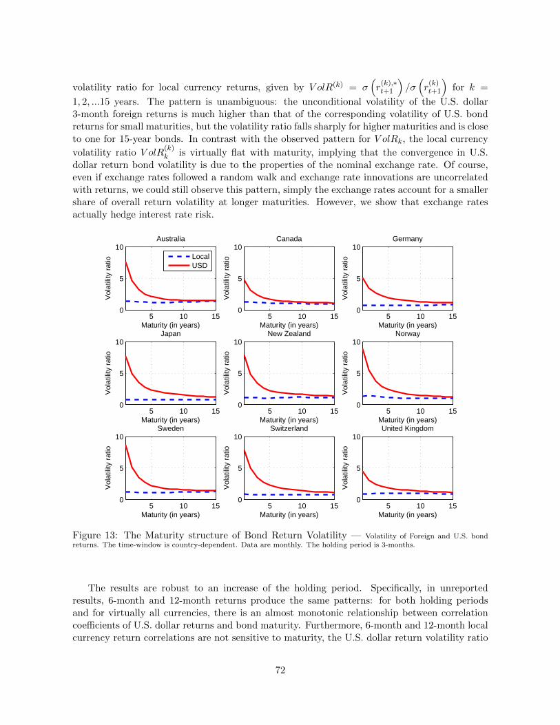
volatility ratio for local currency returns, given by V olR(k) = σ(r

(k),∗t+1

)/σ(r

(k)t+1

)for k =

1, 2, ...15 years. The pattern is unambiguous: the unconditional volatility of the U.S. dollar3-month foreign returns is much higher than that of the corresponding volatility of U.S. bondreturns for small maturities, but the volatility ratio falls sharply for higher maturities and is closeto one for 15-year bonds. In contrast with the observed pattern for V olRk, the local currency

volatility ratio V olR(k)k is virtually flat with maturity, implying that the convergence in U.S.

dollar return bond volatility is due to the properties of the nominal exchange rate. Of course,even if exchange rates followed a random walk and exchange rate innovations are uncorrelatedwith returns, we could still observe this pattern, simply the exchange rates account for a smallershare of overall return volatility at longer maturities. However, we show that exchange ratesactually hedge interest rate risk.

5 10 150

5

10Australia

Maturity (in years)

Vol

atili

ty r

atio

LocalUSD

5 10 150

5

10Canada

Maturity (in years)

Vol

atili

ty r

atio

5 10 150

5

10Germany

Maturity (in years)

Vol

atili

ty r

atio

5 10 150

5

10Japan

Maturity (in years)

Vol

atili

ty r

atio

5 10 150

5

10New Zealand

Maturity (in years)

Vol

atili

ty r

atio

5 10 150

5

10Norway

Maturity (in years)

Vol

atili

ty r

atio

5 10 150

5

10Sweden

Maturity (in years)

Vol

atili

ty r

atio

5 10 150

5

10Switzerland

Maturity (in years)

Vol

atili

ty r

atio

5 10 150

5

10United Kingdom

Maturity (in years)

Vol

atili

ty r

atio

Figure 13: The Maturity structure of Bond Return Volatility — Volatility of Foreign and U.S. bondreturns. The time-window is country-dependent. Data are monthly. The holding period is 3-months.

The results are robust to an increase of the holding period. Specifically, in unreportedresults, 6-month and 12-month returns produce the same patterns: for both holding periodsand for virtually all currencies, there is an almost monotonic relationship between correlationcoefficients of U.S. dollar returns and bond maturity. Furthermore, 6-month and 12-month localcurrency return correlations are not sensitive to maturity, the U.S. dollar return volatility ratio

72

is very high for short maturities, but quickly converges towards one, and the local currencyreturn volatility ratio is flat with maturity.

73

SSRN-id2340547 hotmoneygoround

Documents

Transcript of SSRN-id2340547 hotmoneygoround