SSC-392 PROBABILITY BASED SHIP DESIGN: IMPLEMENTATION …
157
NTIS # PB97-109961 SSC-392 PROBABILITY BASED SHIP DESIGN: IMPLEMENTATION OF DESIGN GUIDELINES This document has been approved For public release and sale; its Distribution is unlimited SHIP STRUCTURE COMMITTEE 1996
Transcript of SSC-392 PROBABILITY BASED SHIP DESIGN: IMPLEMENTATION …

NTIS # PB97-109961
SSC-392
PROBABILITY BASED SHIP DESIGN:
IMPLEMENTATION OF DESIGN GUIDELINES
This document has been approved For public release and sale; its
Distribution is unlimited
SHIP STRUCTURE COMMITTEE 1996


CONVERSION FACTORS (Approximate conversions to metric measures)
To convert from to Function Value LENGTH inches meters divide 39.3701 inches millimeters multiply by 25.4000 feet meters divide by 3.2808 VOLUME cubic feet cubic meters divide by 35.3149 cubic inches cubic meters divide by 61,024 SECTION MODULUS inches2 feet2 centimeters2 meters2 multiply by 1.9665 inches2 feet2 centimeters3 multiply by 196.6448 inches4 centimeters3 multiply by 16.3871 MOMENT OF INERTIA inches2 feet2 centimeters2 meters divide by 1.6684 inches2 feet2 centimeters4 multiply by 5993.73 inches4 centimeters4 multiply by 41.623 FORCE OR MASS long tons tonne multiply by 1.0160 long tons kilograms multiply by 1016.047 pounds tonnes divide by 2204.62 pounds kilograms divide by 2.2046 pounds Newtons multiply by 4.4482 PRESSURE OR STRESS pounds/inch2 Newtons/meter2 (Pascals) multiply by 6894.757 kilo pounds/inch2 mega Newtons/meter2
(mega Pascals) multiply by 6.8947
BENDING OR TORQUE foot tons meter tons divide by 3.2291 foot pounds kilogram meters divide by 7.23285 foot pounds Newton meters multiply by 1.35582 ENERGY foot pounds Joules multiply by 1.355826 STRESS INTENSITY kilo pound/inch2 inch½(ksi√in) mega Newton MNm3/2 multiply by 1.0998 J-INTEGRAL kilo pound/inch Joules/mm2 multiply by 0.1753 kilo pound/inch kilo Joules/m2 multiply by 175.3

TABLE OF CONTENTS
LIST OF SYMBOLS ....................................................................................................... vi
ACKNOWLEDGEMENT............................................................................................... xi
1. INTRODUCTION ......................................................................................................1
1.1 Background .........................................................................................................1 1.2 Advantages of a Probability-Based Design Code ...............................................1 1.3 Objectives of the Project .....................................................................................2 1.4 Organization of the Report ..................................................................................3
2. PROTOTYPE CODE STATEMENT.........................................................................4
2.1 Forward to the Code Statements .........................................................................4 2.2 Planning...............................................................................................................5 2.3 Hull Girder ..........................................................................................................6 2.4 Unstiffened Panel..............................................................................................10 2.5 Stiffened Panel ..................................................................................................16 2.6 Fatigue ...............................................................................................................23
APPENDICES
A LITERATURE REVIEW: STRUCTURAL RELIABILITY AND CODE DEVELOPMENT...............................................................................36
B TARGET RELIABILITIES......................................................................................39
C PARTIAL SAFETY FACTORS (PSF) AND SAFETY CHECK EXPRESSIONS .........................................................................................48
D COMMENTARY: LIMIT STATE FUNCTIONS FOR HULL GIRDER COLLAPSE...................................................................................57
E COMMENTARY: LIMIT STATE FUNCTIONS FOR BUCKLING OF PLATES BETWEEN STIFFENERS............................................61
F COMMENTARY: LIMIT STATE FUNCTIONS FOR STIFFENED PLATES..............................................................................................93
G COMMENTARY: LIMIT STATE FUNCTIONS FOR FATIGUE ...............................................................................................................119
REFERENCES .............................................................................................................142

LIST OF SYMBOLS
A = the sectional area of the longitudinal plate-stiffener combination
AS = sectional area of the longitudinal stiffener only
Atr = transformed area of the longitudinal plate-stiffener combination = bT + AS
A0 = fatigue strength coefficient (NSm = A0); defines design curve a = length or span of plate; the length or span of the panel between transverse webs; the
length of the longitudinal stiffener a/b = aspect ratio of plate B = plate slenderness ratio BP = breadth of the panel b = distance between longitudinal stiffeners bf = stiffener flange breadth C = panel stiffness parameter
Cr = factor by which plate rotational restraint is reduced due to web bending
CS = coefficient of variation of stress; includes modeling error and inherent stress uncertainty; equivalent to CB in Appendix G
c = buckling knock-down factor
c fy z = ultimate moment capacity of the hull D = fatigue damage; plate flexural rigidity, = Et3/12(1-ν2)
dw = stiffener web depth E = modulus of elasticity (Young’s modulus)
Fu = ultimate tensile strength; ultimate strength of plate under uniaxial compressive stress
f = stress
fE = Euler’s buckling stress for the plate-stiffener combination
fE,tr = Euler’s buckling stress for the transformed section
fi = frequency of wave loading in the ith sea-state
fp = proportional limit stress for the stiffener in compression
fS = stress due to stillwater pressure

LIST OF SYMBOLS - continued
fW = stress due to wave pressure
fX = factored extreme axial in-plane compressive stress from hull girder bending
fX,tr = transformed in-plane compressive stress
fx,T = the elastic tripping stress for the beam-column
fy = yield strength
fyp = yield strength of plate
fys = average compressive yield stress of the stiffener
f0 = the average frequency of stress cycles over the service life, NS
f1 = stress in the flange of the stiffener
f2 = stress in the plate flange of the stiffener G = shear modulus g = limit state or performance function
Ipx,Ipy = the moment of inertia of the effective plating (alone) about the neutral axis of the combined plate and stiffener, in the longitudinal & transverse directions, respectively
Isp = polar moment of inertia of stiffener about center of rotation
Isz = moment of inertia of the stiffener only about an axis through the centroid of the stiffener and parallel to the web
Ix, = the moment of inertia of the plate-stiffener combination, longitudinal
Ix,Iy = the moment of inertia of the combined plate and stiffener, longitudinal & transverse
Itr = the moment of inertia of the transformed longitudinal plate-stiffener combination J = St. Venant’s torsional constant k = buckling coefficient for a simply-supported plate under uniaxial in-plane load kD = load combination factor that accounts for phase angle for dynamic loads
kW = load combination factor that accounts for phase angle for wave loads
kw,kd = load combination factors

LIST OF SYMBOLS - continued
k1,k2 = coefficients that depend on the aspect ratio a/b
Md = extreme dynamic (slamming or springing induced) hull girder bending moment (nominal)
Ml = plastic moment of longitudinal stiffener at center
Ms = stillwater hull girder bending moment (nominal)
Mt = plastic moment of transverse stiffener at center
Mu = ultimate moment capacity
= c fy z
Mw = extreme wave induced hull girder bending moment (nominal)
M0 = max bending moment in a simply-supported beam under a uniform lateral load
m = negative reciprocal slope of the S-N curve; fatigue strength exponent (NSm = A0); number of longitudinal stiffeners; number of longitudinal half-waves for stiffener tripping
N = number of longitudinal sub-panels in overall (or gross) panel NS = fatigue stress cycles experienced during intended service life of ship
NSX,NSY = ultimate longitudinal and transverse in-plane load from the stillwater hull girder bending moment, respectively
NWX,NWY = ultimate longitudinal and transverse in-plane load from the wave hull girder bending moment, respectively
n = number of transverse stiffeners P = pressure PS = stillwater hydrostatic pressure
Ps = extreme lateral pressure due to stillwater condition
PW = wave hydrostatic pressure
Pw = extreme lateral pressure due to wave action
P1 = factored lateral pressure applied to the stiffened panel (Mode I)
P2 = factored lateral pressure applied to the stiffened panel
pf = probability of failure R = strength of plate under lateral pressure

LIST OF SYMBOLS - continued
Se = equivalent constant amplitude stress (Miner’s stress); nominal stress at a detail
Sm = maximum allowable stress peak to satisfy fatigue requirement
Sp = design stress; stress peak which is exceeded, on the average, once during NS cycles (Sp = S0/2)
S0 = stress range which is exceeded, on the average, once during NS cycles T = transformation factor based on secant modulus concept t = plate thickness tf = stiffener flange thickness
tw = stiffener web thickness
yf = distance from the centroidal axis of the cross-section to the mid-thickness of the stiffener flange
yp,tr = distance from the centroidal axis of the transformed cross section to the mid-thickness of the plating
Z = hull girder section modulus to the location of interest z = section modulus; section modulus at the compression flange (at deck in sagging or
at bottom in hogging condition) α = plate aspect ratio β = safety index (reliability index) β0 = target safety index
∆ = the initial eccentricity of the beam-column, typically taken as a/750 ∆p = eccentricity of load due to use of transformed section
∆0 = target damage level, maximum allowable value of D δ = length of the transferse stiffener
δ0 = the central deflection of a simply-supported beam under a uniform lateral load Γ = gamma function, Γ(x) = (x - 1)!. (Note that non- integer factorials can be computed
from many electronic calculators) Φ = cumulative distribution function for standard normal; magnification factor for in-
plane compressive loading φ = partial safety factor for strength
LIST OF SYMBOLS - continued
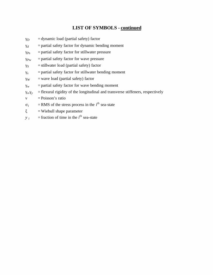
γD = dynamic load (partial safety) factor
γd = partial safety factor for dynamic bending moment
γPs = partial safety factor for stillwater pressure
γPw = partial safety factor for wave pressure
γS = stillwater load (partial safety) factor
γs = partial safety factor for stillwater bending moment
γW = wave load (partial safety) factor
γw = partial safety factor for wave bending moment
γx,γy = flexural rigidity of the longitudinal and transverse stiffeners, respectively ν = Poisson’s ratio
σi = RMS of the stress process in the ith sea-state
ξ = Wiebull shape parameter ψ i = fraction of time in the ith sea-state

ACKNOWLEDGMENT
This work was sponsored by the interagency Ship Structure Committee, under Contract No. DTCG 23-94-C-E01026. The authors are grateful for the guidance of the Project Technical Committee, especially the Chairman, William Richardson of the Naval Surface Warfare Center, Carderock Division.

1. INTRODUCTION
1.1 Background
The design of a marine structure depends upon predicted loads and the structure’s calculated capacity to resist them. There is always significant uncertainty in determining either. Historically, the engineering design process has compensated for these uncertainties by experience and subjective judgment. However, with reliability technology, these uncertainties can be considered more quantitatively. Specifically, the use of probability-based design criteria, or safety check expressions, has the promise of producing better engineered designs. For a naval surface ship, implementation of a probability-based design code can produce ship structure having, relative to structure designed by current procedures, (1) a higher level of reliability, or (2) lower overall weight, or (3) both.
The historical development of design criteria based on reliability analysis is described in the literature review of Appendix A. Directly relevant to this program is the probability-based Load and Resistance Factor Design (LRFD) procedure issued by the American Institute for Steel Construction (AISC) in 1986. Further, the American Petroleum Institute (API) has extrapolated this technology for offshore structures with RP2A-LRFD, also in 1989, with a draft “Recommended Practice for Design, Fabrication and Installation of Fixed Offshore Structures.” A review of the various possible formats for probability-based design criteria is presented in Appendix A, but the same partial safety factor approach used here is similar to those in the AISC and API work.
1.2 Advantages of a Probability-Based Design Code
Relative to a conventional factor of safety code, a probability-based design code has the promise of producing a better engineered structure. Specific benefits are well documented in the literature (see Appendix A).
1. A more efficiently-balanced design results in weight savings and/or an improvement of reliability.
2. Uncertainties in the design are treated more rigorously.
3. Because of an improved perspective of the overall design process, development of probability-based design procedures can stimulate important advances in structural engineering.
4. The codes become a living document. They can be easily revised periodically to include new sources of information and to reflect additional statistical data on design factors.
5. The partial safety factor format used herein also provides a framework for extrapolating existing design practice to new ships where experience is limited.
The bottom line is that experience has shown that adoption of a probability-based design code has resulted in significant savings in weight. The jury is still out on reliability improvements, although the new codes are specifically designed so that the reliability is equal to or better than the older codes they replace. Experiences are not well documented at this time, but designers have commented that, relative to the conventional working stress code, the new AISC-
LRFD requirements are saving anywhere from 5% to 30% steel weight, without about 10% being typical. This may or may not be the case for ships and other marine structures.
1.3 Objectives of the Project
The objective of this project is to provide a demonstration of a probability-based design code for ships. A specific provision of the code will be a safety check expression, which, for example, for three bending moments (stillwater Ms, wave Mw, and dynamic Md), and strength, Mu, might have the form, following the partial safety factor format of AISC and API,
γs Ms + γw M w + γd M d ≤ φ Mu (1.1)
γs, γw, γd, and φ are the partial safety factors. The design variables (M’s) are to be taken at their nominal values, typically values in the safe side of the respective distributions. Other safety check expressions for hull girder failure that include load combination factors as well as consequence of failure factors are considered in Appendix D. This report provides demonstrations of safety check expressions for several components and failure modes.
Development of a comprehensive structural code would require the following considerations:
1. Definition of all of the provisions of the code, which components and failure modes should be included.
2. Definition of the limit state function associated with each provision of the code. This would include:
(a) specific considerations of load combinations (b) considerations of stress and strength modeling error (c) statistical distributions of all design factors (d) the relationship between a nominal design or characteristic value of a design
factor and its distribution
3. Definition of the format of the safety check expressions. A partial safety factor format will be employed in this study.
4. Definition of the target reliabilities for the important provisions of the code.
5. Method of establishing the partial safety factors. In problems such as fatigue (typically), a lognormal format can be employed and a closed-form expression for the safety factor can be derived. For the more general case, one of the available reliability computer programs can be used.
6. Development of the prototype code statements.
It is the objective of this project to provide a road map for the development of a full code, demonstrating important components of the process.
1.4 Organization of the Report
The report is organized so that the prototype code statement is the centerpiece. Peripheral reference material is provided in the Appendices. Code requirements for (1) ultimate strength of

hull girder, a stiffened panel, an unstiffened panel, and (2) fatigue of select welded detail are presented for two ship types: (1) a tanker, and (2) a cruiser.
The main body of the report is a presentation of the prototype code. Section 2 is the prototype code statements for the tanker and the cruiser.
Appendices contain all of the background and supporting material:
A Literature Review: Structural Reliability and Code Development B Target Reliabilities C Partial Safety Factors (PSF) and Safety Check Expressions D Commentary: Limit State Functions for Hull Girder Collapse E Commentary: Limit State Functions for Buckling of Plates Between Stiffeners F Commentary: Limit State Functions for Stiffened Plates G Commentary: Limit State Functions for Fatigue

2. PROTOTYPE CODE STATEMENT
2.1 Forward to the Code Statements
While complete design criteria documents for the tanker and the cruiser would be separate, requirements are combined in this prototype code. The reason for this presentation is for pedagogical purposes. The authors believe that the reader will have a better understanding of the process if specific tanker and cruiser requirements are presented side-by-side.
The comentary that follows was inspired by API-RP2A-LRFD (1989), the probability-based design requirement for fixed offshore drilling and production platforms.
2.1.1 Scope
The partial safety factor (PSF) format (similar to LRFD) of this practice is reliability-based. Uncertainties that naturally occur in the determination of loads and member strengths are explicitly accounted for in the development of this format. While load and resistance factors have been chosen based on reliability considerations, the designer is not faced with carrying out probabilistic calculations. This work has been done in the development of code statements, as documented in the Appendices. The code statements are intended for design of new ships and not for reanalysis of existing ships or for maintenance decisions.
The PSF approach explicitly accounts for load and resistance uncertainties and thereby achieves more uniform reliability. Loads are modified by factors chosen on the basis of the load uncertainties. Similarly, calculated resistances are reduced by a factor that accounts for the uncertainty associated with the predictability of the failure mechanism.
2.1.2 Target Reliability
Target reliabilities were chosen on the basis of:
(1) reliability analysis of existing ship structure (SR-1344, among others)
(2) prior reliability analysis of ship structure and structural components
(3) use of target values in related applications
(4) the application of professional judgment
The choice of a target reliability is, in part, based on consideration of the consequences of failure. For example, the hull girder should have a higher reliability relative to collapse than a fatigue detail relative to crack initiation.
2.2 Planning
2.2.1 General Comments
The initial plnning for the ship should include the determination of all criteria upon which the design of the ship will be based. Design criteria, as used herein, include all operational requirements and environmental criteria which could affect the design of the ship.

2.2.2 Operational Considerations
Tanker. While the principal role of the tanker is to transport crude oil, any possible unusual operational requirements during the service life should be considered. This might include possible changes of cargo or structural modifications. The operational profile of the ship, such as route, speed, and headings also plays an important role.
Cruiser. While the principal role of the cruiser is to support military operations, any possible unusual requirements during the service life should be considered. This might include possible structural modifications. The operational profile of the ship, such as route, speed, headings, etc., also plays an important role.
2.2.3 Environmental Considerations
(1) Normal oceanographic and meteorological environmental conditions to which the vessel is exposed over the service life are needed.
(2) Extreme oceanographic and meterological environmental conditions to which the vessel is exposed over the service life are required to develop the extreme environmental load.
Wind driven waves are the principal source of environmental forces on the vessel. The heading of the ship relative to the waves, the speed of the ship and the cargo loading condition are significant to structural loads and should be considered in the process of defining design loads.
2.2.4 Factors
The factors to be considered in selecting design criteria are:
(1) Safety of life at sea
(2) Ability of the ship to carry out its assigned mission, particularly for naval vessels
(3) Possibility of detrimental pollution and other consequences of failure
(4) Requirements of classification societies or regulatory agencies
(5) Ability to define operational and extreme environmental conditions
(6) Ability to perform the structural analysis given the environmental conditions
(7) Ability to predict ultimate and fatigue strengths
(8) The probability of occurrence of unusual and potentially damaging events, e.g., iceberg impact
(9) The probability of human error in navigation
(10) Error in meteorological forecasts, storm avoidance, and routing
2.3 Hull Girder
2.3.1 Definitions of Terms
c fy z = ultimate moment capacity of the hull
Ms = hog or sag stillwater bending moment (nominal)

Mw = hog or sag wave bending moment (nominal)
Md = dynamic (slamming or springing) bending moment (nominal)
kw,kd = load combination factors
fy = yield strength (nominal) z = section modulus c = buckling knock-down factor
γs = partial safety factor for stillwater bending moment
γw = partial safety factor for wave bending moment
γd = partial safety factor for dynamic bending moment
φ = partial safety factor for yield strength
2.3.2 Preliminary Remarks
This section provides the requirements to avoid failure of the hull girder. To perform a safety check, it is necessary to provide the following information.
2.3.3 Hull Girder Bending Moments
Hull girder bending moments consist of stillwater bending moment Ms, wave beiding moment, Mw, and dynamic bending moment, Md. The dynamic bending moment is either a slamming or springing moment. The values of these moments to be used in the following safety check for hull ultimate limit state are nominal va lues defined as follows.
Ms is the maximum value of the stillwater bending moment resulting from the worst loading condition of the ship, in both hogging and sagging modes. For commercial ships, a default value for Ms may be taken as the maximum allowable stillwater bending moment permitted by Classification Societies for the ship under consideration. Both hogging and sagging modes, and the associated stillwater bending moments, should be examined using the safety checks given in Section 2.3.6.
The wave bending moment, Mw, is the mean value of extreme wave bending moments the ship is likely to encounter during its lifetime. Mw can be calculated on the basis of short-term analysis, where the ship is assumed to encounter a storm of specific duration (three to five hours) and with certain small encounter probability. Alternatively, long-term analysis may be used to determine Mw based on the operational profile of the ship in different sea-states and encounter probabilities. In both cases, short- and long-term analysis, a linear strip theory ship motion program may be used with adjustment made for hog/sag difference in the bending moment. A second-order strip theory ship motion program, which distinguishes between hog and sag moments, may also be used to determine Mw.
Md is the mean value of the extreme dynamic bending moment amplitude. Md can be either due to springing or slamming. In either case, Md is to be calculated based on a specialized computer program under the same conditions (e.g., sea-states) Mw was computed. The hull flexibility must be taken into consideration. Normally, springing is not important in very high

sea-states. As default values for slamming, Md may be taken as the values provided by Classification Societies, if any, or as 20% of Mw for commercial ships and 30% of Mw for Naval vessels, both in sagging condition. In hogging condition, Md for slamming may be taken as zero.
In the proceeding safety check inequality, all values of the bending moments should have the same sign, i.e., all sagging or all hogging bending moments.
2.3.4 Yield Strength of the Material
fy, which appears in the proceeding safety check, is the “minimum” nominal value of the yield strength of the material. If this value is not known, a default value of the minimum specified yield strength, as provided by Classification Society rules, may be used in the safety check inequality.
2.3.5 Other
kw, which appears in the proceeding safety check, is a load combination factor between the stillwater bending moment and the combined wave and dynamic moments. This factor depends on the magnitudes of combined wave and dynamic moments associated with different values of stillwater moments. Because of the manner the stillwater bending moment is defined in the safety check, a default value of kw may be taken as one.
kd is a load combination factor between the wave and dynamic bending moments. Its value depends on the correlation coefficient between these two moments, which can be determined on the basis of dynamic analysis of a ship in a seaway. A default value of kd may be taken as 0.7. For more information on kd, please see Ship Structure Committee Report SSC 373 (1994) or Mansour (1995).
“c,” which appears in the safety check inequality, is a buckling knock-down factor. It is equal to the ultimate collapse bending moment of the hull, taking buckling into consideration, divided by the initial yield moment. The ultimate collapse moment can be calculated using a nonlinear finite element program, USN “ULTSTR” or using a software based on the Idealized Structural Unit Method (see, e.g., Ueda et al., 1984). Approximate nonlinear buckling analysis may also be used. The initial yield moment is simply equal to the yield strength of the material multiplied by the section modulus of the hull at the compression flange, i.e., at deck in sagging condition, or at bottom in hogging condition. The default values for the buckling knock-down factor “c” may be taken as 0.80 for mild steel and 0.60 for high-strength steel.
2.3.6 Safety Check for Hull Girder Ultimate Limit State
The requirement for a safe design relative to the hull girder ultimate limit state is,
zM k M k M
c fs s w w w d d d
y
>+ +γ γ γ
φ( )
(2.3.1)
The partial safety factors are provided in Table 2.3.1 for the tanker and in Table 2.3.2 for the cruiser. These factors were derived using reliability methods, as described in Appendix C.
Correlation of the variables is taken into consideration through the load combination factors kd and kw.
Note that this is not a complete code requirement for this failure mode. Wider ranges of µd/µw, kw, and kd should be considered.
Although Tables 2.3.1 and 2.3.2 are meant to give “standardized” partial safety factors under the general conditions stated above, Appendix C may be used to obtain partial safety factors under other conditions.

Table 2.3.1 Partial Safety Factors for Tanker: Hull Girder Collapse
φ 0.97
γs 0.80
γw 1.48
γd 1.12
Conditions:
1) Valid for 0.38 < µs/µw < 0.56, where µs and µw are the mean wave and stillwater bending moments in hogging and in sagging condition.
2) Based on µd /µw = 0.20, where µd is the mean dynamic bending moment.
3) Factors: kw = 1.0 kd = 0.70
4) c =−
0 600 80..
for high strength steelfor mild steel
Table 2.3.2 Partial Safety Factors for Cruiser: Hull Girder Collapse
φ 0.95
γs 0.76
γw 1.86
γd 1.30
Conditions:
1) Valid for 0.25 < µs/µw < 0.33, where µs and µw are the mean wave and stillwater bending moments in hogging and in sagging condition.
2) Based on µd /µw = 0.30, where µd is the mean dynamic bending moment.
3) Factors: kw = 1.0 kd = 0.70
4) c =−
0 600 80..
for high strength steelfor mild steel

2.4 Unstiffened Panel
2.4.1 Definitions of Terms a = length or span of plate a/b = aspect ratio of plate such that a ≥ b b = distance between longitudinal stiffeners that define the ends of the plate B = plate slenderness ratio E = modulus of elasticity f = stress fS = stress due to stillwater pressure
fW = stress due to wave pressure
fyp = yield strength (stress) of plate
Fu = strength of plate under uniaxial compressive stress g = limit state or performance function k1,k2 = coefficients that depend on the aspect ratio a/b
kW = load combination factor that accounts for phase angle for wave loads
kD = load combination factor that accounts for phase angle for dynamic loads P = pressure PS = stillwater hydrostatic pressure
PW = wave hydrostatic presure R = strength of plate under lateral pressure t = thickness of plate α = plate aspect ratio β = target reliability index φ = strength (partial safety) factor
γS = stillwater load (partial safety) factor
γW = wave load (partial safety) factor
γD = dynamic load (partial safety) factor ν = Poisson’s ratio
2.4.2 Preliminary Remarks
The limit states for the strength of plates between stiffeners are defined in Section E.2. The limit states can be classified into serviceability and strength types. In Section E.3, two limit states were selected for the development of partial safety factors, one limit state of the serviceability type, and one of the strength type. The prototype code for stiffened panels is based on these two cases.

2.4.3 Serviceability (Stress) Limit State for Plates under Lateral Pressures
2.4.3.1 Load
The following two types of lateral pressure (i.e., normal to the plate) can be computed based on service conditions:
1. Service hydrostatic pressure (P1) due to S and W P1 = PS + PW
2. Service green-seas pressure (P2) due to GS P2
These pressure types do not include dynamic effects. The stress (f) in a plate can be computed as
f k Pbt
k Pbt
k k Pbt
=
+
−
1
2 24
22 2
4
1 22
4
(2.4.1)
where k1 and k2 = coefficients that depend on the aspect ratio of a plate (a/b, such that a≥b, as shown in Fig. 2.4.1) and its boundary conditions, t = plate thickness, and P = either P1 or P2. Values for k1 and k2 are shown in Table 2.4.1. The stress (f) load effect can be computed for either the hydrostatic pressure or the green-seas pressure.
PlatePressurenormal toplate
a
b
Figure 2.4.1 Plate Under Lateral Pressure
Table 2.4.1 Values of k1 and k2
a/b 1.0 1.2 1.4 1.6 1.8 2.0 3.0 4.0 5.0 ∞ k1 0.2674 0.3003 0.3030 0.2981 0.2676 0.2796 0.2435 0.2321 0.2290 0.2250
k2 0.2674 0.3762 0.4530 0.5172 0.5688 0.6102 0.5134 0.7410 0.7476 0.7500
2.4.3.2 Definition of Nominal Values
fyp is the nominal yield strength of the plate. This is the catalog value of yield strength.
The nominal stillwater hydrostatic pressure, PS, and the nominal wave induced hydrostatic pressure, PW, are taken as the mean (annual extreme) values.
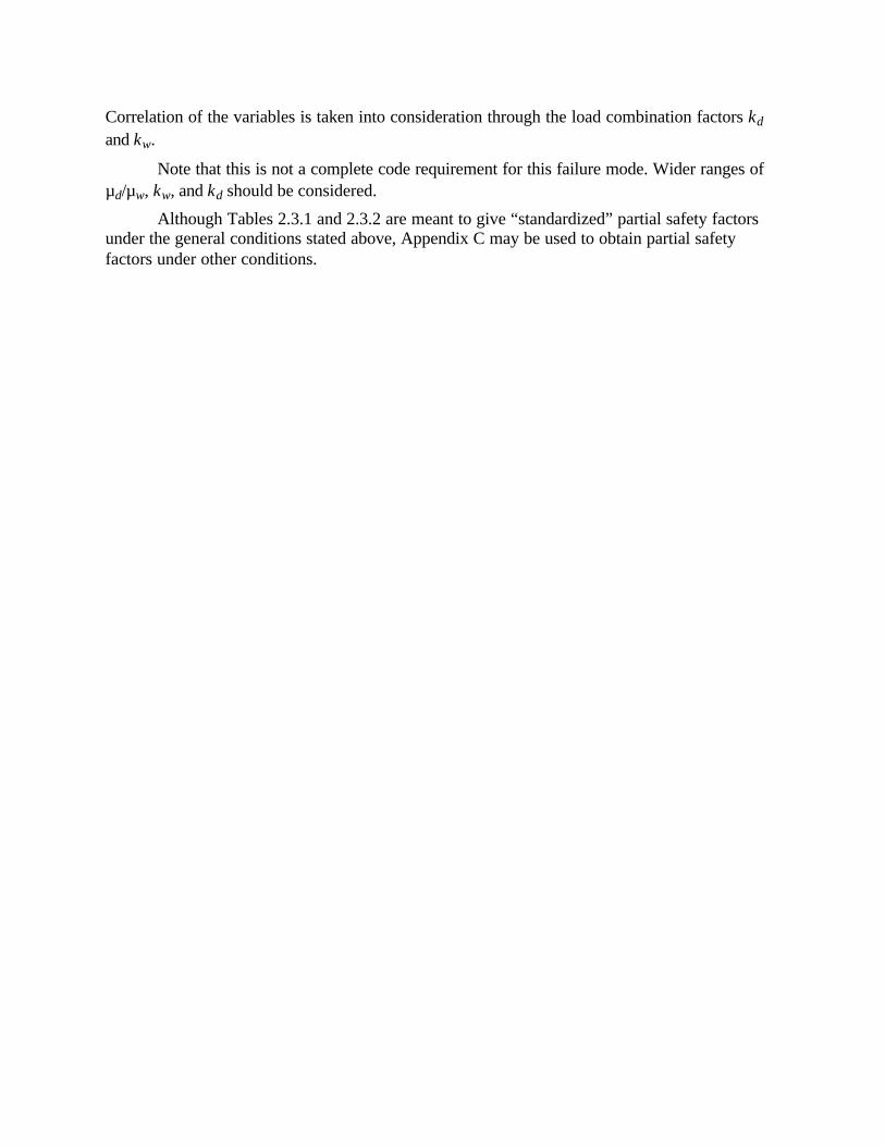
2.4.3.3 Limit State
Partial safety factors should be used to design plates to meet the serviceability condition of first yield at the center of a simply supported plate by satisfying the following safety checking equation:
φ γ γf
bt
k k k k
P PypS S W W
+ −
≥ +2
12
22
1 2
(2.4.2)
The partial safety factors are given for the tanker in Table 2.4.2 and for the cruiser in Table 2.4.3.
Table 2.4.2 Partial Safety Factors for Yielding of Plate
Under Lateral Pressure*: Tanker
φ 0.82
γs 1.37
γw 1.08
*based on a target safety index of 3.0
Table 2.4.3 Partial Safety Factors for Yielding of Plate
Under Lateral Pressure*: Cruiser
φ 0.79
γs 1.42
γw 1.11
*based on a target safety index of 3.5
2.4.4 Uniaxial Compressive Stress on Plates
2.4.4.1 Load Effect
The stress, f, is a function of extreme stillwater loads S, and extreme wave loads W, and can be computed as
f = fS + fW (2.4.3)

2.4.4.2 Strength
The strength Fu of a plate subjected to uniaxial compression parallel to the dimension a, as shown in Fig. 2.4.2, is given by one of the following two cases:
Platein-planecompression
a
b
Figure 2.4.2 Plate Subjected to In-Plane Compression

1. For a/b ≥ 1.0
Ff
B
B B
if B
if B
if B
u
yp
=
−
−
≥
≤ <
<
πν
2
2 2
2
3 1
2 25 1 25
1 0
3 5
1 0 3 5
1 0
( )
. .
.
.
. .
.
(2.4.4)
2. For a/b < 1.0
Ff
CB
u
ypu= + − +
≤α α0 08 1 11
102
2
. ( ) . (2.4.5)
where
C
B
B B
if B
if B
if B
u =
−
−
≥
≤ <
<
πν
2
2 2
2
3 1
2 25 1 25
1 0
3 5
10 3 5
10
( )
. .
.
.
. .
.
(2.4.6a)
α = a/b (2.4.6b)
and
Bbt
f
Eyp= (2.4.6c)
2.4.4.3 Definition of Nominal Values
fyp is the nominal yield strength of the plate. This is the catalog value of yield strength.
The nominal stillwater induced stress, fS, and the nominal wave induced stress, fW, are taken as the mean extreme values.
2.4.4.4 Limit States for the Load Combination of Stillwater and Wave Loads
Partial safety factors should be used to design plates to meet a strength limit state for plates under uniaxial compression by satisfying the following safety checking equation:
φFu ≥ γS fS + γW fW (2.4.7)
where Fu is computed according to Eqs. (2.4.4) through (2.4.6).

Table 2.4.4 Partial Safety Factors for Plate with
Uniaxial Compressive Stress*: Tanker
φ 0.88
γs 1.30
γw 1.25
*based on a target safety index of 3.0
Table 2.4.5 Partial Safety Factors for Plate with
Uniaxial Compressive Stress*: Cruiser
φ 0.88
γs 1.30
γw 1.40
*based on a target safety index of 3.5
2.4.4.5 Limit States for the Load Combination of Stillwater, Wave, and Dynamic Loads
Partial safety factors should be used to design plates to meet a strength limit state for plates under uniaxial compression by satisfying the following safety checking equation:
φFu ≥ γS fS + kW (γW fW + kD γD fD) (2.4.8)
where Fu is computed according to Eqs. (2.4.4) through (2.4.6). The stillwater and wave stresses, in this case, need to be based on the mean lifetime extreme loads, as defined in Section 2.4.
The partial safety factors are given in Table 2.4.6 for the tanker and Table 2.4.7 for the cruiser.
Table 2.4.6 Partial Safety Factors for Plate with
Uniaxial Compressive Stress, Including Dynamic Effects: Tanker*
φ 0.77
γs 0.75
γw 1.50
γd 1.27

*based on a target safety index of 3.0, kw = 1.0, kd = 0.7
Table 2.4.6 Partial Safety Factors for Plate with
Uniaxial Compressive Stress, Including Dynamic Effects: Cruiser*
φ 0.74
γs 0.75
γw 1.50
γd 1.27
*based on a target safety index of 3.5, kw = 1.0, kd = 0.7
2.5 Stiffened Panels
2.5.1 Definitions of Terms Used for Stiffened Panels A = the sectional area of the longitudinal plate-stiffener combination
AS = sectional area of the longitudinal stiffener only
Atr = transformed area of the longitudinal plate-stiffener combination
= bT+AS a = the length or span of the panel between transverse webs B = the plate slenderness ratio
BP = breadth of the panel b = distance between longitudinal stiffeners
bf = stiffener flange breadth C = panel stiffness parameter dw = stiffener web depth E = Young’s modulus Fu = plate collapse strength in terms of applied stress
fE,tr = Euler’s buckling stress for the transformed section
fX = factored extreme axial in-plane compressive stress from hull girder bending (Eq. (2.5.8a))
fX,tr = transformed in-plane compressive stress
f2 = stress in the plate flange of the stiffener
fyp = yield stress of the plate material

Ix,Iy = the moment of inertia of the plate-stiffener combination, longitudinal & transverse
Itr = the moment of inertia of the transformed longitudinal plate-stiffener combination
kw,kd = load combination factors
M0 = max bending moment in a simply supported beam under a uniform lateral load (Eq. (2.5.9b))
Ms = stillwater hull girder bending moment (nominal)
Mw = extreme wave induced hull girder bending moment (nominal)
Md = extreme dynamic (slamming or springing induced) hull girder bending moment (nominal)
Mp = full plastic moment for beam in bending N = number of longitudinal sub-panels in overall (or gross) panel n = number of longitudinal stiffeners in gross panel
Ps = extreme lateral pressure due to stillwater condition
Pw = extreme lateral pressure due to wave action
P2 = factored lateral pressure applied to the stiffened panel (Eq. (2.5.9a)) T = transformation factor based on a secant modulus concept (Eq. (2.5.5)) t = plate thickness
tf = stiffener flange thickness
tw = stiffener web thickness
yp,tr = distance from the centroidal axis of the transformed cross section to the mid-thickness of the plating
Z = hull girder section modulus to the location of interest z = section modulus of the beam-column ∆ = the initial eccentricity of the beam-column, typically taken as a/750
∆p = eccentricity of load due to use of transformed section
δ0 = the central deflection of a simply supported beam under a uniform lateral load (Eq. (2.5.9b))
Φ = magnification factor for in-plane compressive loading φ = strength reduction partial safety factor γs = partial safety factor for stillwater bending moment
γw = partial safety factor for wave bending moment
γd = partial safety factor for dynamic bending moment
γPs = partial safety factor for stillwater pressure
γPw = partial safety factor for wave pressure

2.5.2 Preliminary Remarks
This section provides the requirements to avoid failure of a stiffened panel. Six limit states were identified as important in determining the strength of a stiffened panel. Three are associated with the overall (or gross) panel and three are associated with the longitudinally stiffened sub-panel. In general, if the transverse stiffeners on the stiffened panel provide enough flexural rigidity, the strength of the longitudinally stiffened sub-panel will be the controlling factor in the strength of the stiffened panel. A more thorough discussion of the limit states is provided in Appendix F.
For the purpose of demonstrating a reliability-based code, two limit states are discussed in the following. Both limit states are checking limit states. That is, they are used to check the adequacy of the scantlings developed by another means. To perform the safety checks for these two limit states, it is necessary to provide the following information.
2.5.3 Loads
The stiffened panels are subjected to both in-plane stresses and lateral pressure. The limit states under consideration here are ultimate limit states in which the in-plane stresses are compressive. Those stresses are developed due to the hull girder bending moments.
The hull girder bending moments are defined in Section 2.4.3. The nominal values for all of the bending moments should be used. If results from ship motions programs or model testing are not available, the default values for Ms, Mw, and Md, as given in Section 2.4.3, may be used. In the following calculations, all values of bending moment should have the same sign, i.e., all should be sagging or all should be hogging bending moments.
The stillwater pressure applied to the panel, Ps, is simply the pressure due to the average hydrostatic head acting on the panel from all of the loading conditions expected during the lifetime of the ship. For panels in the ships bottom, the hydrostatic head is simply the average draft of the ship over its lifetime. For panels in the deck, the stillwater pressure is zero.
The wave induced pressure, Pw, is the mean value of the extreme wave which is taken onboard. This value can be determined from the number of occurrences of green-seas on deck based on a short-term analysis, where the ship is assumed to encounter a storm of a specified duration and with a certain small probability of occurrence. Alternatively, a long-term analysis may be used in which an operational profile for the ship is developed. Both cases, short- and long-term analysis, require either a ship motions program analysis or model testing to develop the needed information. As defaults, the Classification Societies values for wave induced hydrostatic pressure may be used for Pw.
2.5.4 Material Properties
The modulus of elasticity and Poisson’s ratio for the material used must be specified. The average compressive yield stress of the plating, fyp, is also required. If this value is not known, a default, specified by the Classification Societies, may be used in the checking equations.

2.5.5 Geometric Properties
In order to evaluate the strength of the stiffened panel, the scantlings of the stiffeners and plating that make up the panel must be known. The web height and thickness and the flange width and thickness of both the longitudinal and transverse stiffeners must be known. A typical longitudinal stiffener is shown in Figure 2.5.1, with the required dimensions identified. Similar dimensions for the transverse stiffener (or web frame) are also needed. Nominal values from the manufacturers’ specifications are suitable for use in the safety check equations. Based on these dimensions, the parameters which characterize the flexural and axial stiffness of the stiffeners can be determined.
bf
tf
tw
dw
t
b
Figure 2.5.1 Geometry Definitions
2.5.6 Other
The two load combination factors, kw and kd, depend on the magnitudes of the wave and dynamic moments associated with the stillwater and wave moments, respectively. Section 2.3.5 and Appendix B provide further discussion on determining the values to use for these factors. If model test data or a seekeeping program is not available, default values of kw = 1.0 and kd = 0.7 may be used.
2.5.7 Safety Check for Stiffened Panel Limit State
The purpose of this expression is to ensure that the size of the transverse stiffeners is sufficient to prevent buckling of the overall (or gross) stiffened panel. The safety check equation can be stated as:

I a
I b
B
C a ny
x
p≥ +
4
2 41
1π
(2.5.1)
where Bp is the width of the gross panel, a is the length of a single panel, n is the number of longitudinal stiffeners, and C is a parameter which depends on the number of longitudinal spans in the gross panel.
CN
= +0 252
3. (2.5.2)
Here, N is the number of longitudinal panels in the overall panel.
2.5.8 Safety Check for the Mode II Collapse of the Longitudinally Stiffened Sub-Panel
The combination of in-plane compression and positive bending (putting the stiffener flange in tension) gives rise to the possibility of what is referred to as a Mode II failure mechanism. With small or moderate lateral loads (M0 / Mp ≈ 0.7 or less), collapse occurs dur to compression failure of the plating. If the plate were to remain perfectly elastic through the range of loading, the analysis would be that for a simple beam-column. However, for most welded plating, the compressive collapse is a complex inelastic process. This is due, in part, to the presence of residual stresses due to welding.
To ensure that the stiffeners and plating are of sufficient size to prevent a Mode II collapse of the longitudinally stiffened sub-panel, the following limit state should be checked
φ Fu ≥ f2 (2.5.3)
Values of φ, the strength reduction partial safety factor, for different conditions are provided in Table 2.5.1. The strength term in Eq. (2.5.3) is defined as follows:
Table 2.5.1 Partial Safety Factors for Mode II Limit State
DECK STRUCTURE BOTTOM STRUCTURE
CRUISER TANKER CRUISER TANKER
γPs 0 0 1.40 1.40
γPw 1.10 1.10 1.10 1.10
γs 0.76 0.80 0.76 0.80
γw 1.86 1.48 1.86 1.48
γd 1.30 1.12 1.30 1.12
φ 0.54 0.59 0.54 0.59

FT
Tfu yp=
− 01. (2.5.4)
The transformation factor, T, is based on the secant modulus concept to account for the actual end shortening curve of welded steel plating (Hughes, 1980). The transformation factor is given as
TB
= + − −
0 25 2
10 422..
ξ ξ (2.5.5)
The terms in Eq. (2.5.5) are primarily functions of the plate strength. B is the plate slenderness ratio and is simply a factor which relates slenderness ratio to the plate yield stress. They are defined as
ξ = + =12 75
2
.B
Bbt
f
Eyp (2.5.6)
The load effect for this limit state is the compressive stress in the plate flange of the stiffener (f2) which results from the combination of applied pressure and axial compressive stress. The expression for f2 is (Hughes, 1988):
f fMz
f Az
f A
zX trp tr
X tr tr
p tr
X tr tr p
p tr2
0 0= + ++
+,,
,
,
,
,
( )δ ∆Φ
∆ (2.5.7)
where
zp,tr = section modulus of the combined stiffener and transformed plating to the plating. The plating has a thickness t and a width btr
btr = transformed plate width, = T × b ∆ = initial deflection, default is a/750
∆p = induced eccentricity,
h AA As
tr
1 1−
h = distance from midplane of the plating to the centroid of the stiffener As = sectional area of the stiffener only
A = sectional area of combined stiffener and plating (As + b t)
Atr = sectional area of transformed section (As + btr t)
Φ = magnification factor
= 1
1
2
2
−=
ff
fE I
A aX tr
E tr
E trtr
tr,
,
,whereπ

The load terms in Eq. (2.5.7) come from factored loads based on Sections 2.3.5 and 2.5.3. The in-plane compressive applied stress is found from
fM k M k M
ZXs s w w w d d d=
+ +γ γ γ( ) (2.5.8a)
f fAAX tr X
tr, =
(2.5.8b)
P2 = γPs Ps + kw (γPw Pw) (2.5.9a)
MP ba P a
E Itr0
22
02
4
8 384= =δ (2.5.9b)
Values for the load amplification partial safety for both moment and pressure are provided in Table 2.5.1.
2.6 Fatigue
2.6.1 Preliminary Remarks
Generally, it is assumed that the welded joints are more vulnerable to fatigue failure than the base material. Thus, relative to fatigue, attention should be focused on, but not restricted to, the welded interfaces between members.
In design for fatigue avoidance, one of two fatigue strength models can be used: (1) the characteristic S-N curve based on fatigue test data, and (2) the fracture mechanics approach based on crack growth data. For welded joints, it is assumed that the initiation phase is negligible and that life can be predicted using the fracture mechanics approach [Gurney (1979), Fatigue Handbook (1985)]. Because it is generally considered that the fracture mechanics approach is more refined, it will be used for, but not restricted to, components and detail for which the consequences of failure are relatively large. In this limited prototype code, only the S-N approach is considered.
NOTE: Fatigue stresses are assumed to be the nominal stresses in a joint. See also Section G.2.1 for a discussion of the hot spot stress approach.
Relative to the consequences of failure, i.e., the importance of a given member or detail, each component is to be considered in one of three categories:
Category 1 A significant fatigue crack is not considered to be dangerous to (Not Serious) the crew, will not compromise the integrity of the ship structure, will not result in pollution; repairs should be relatively inexpensive.
Category 2 A significant fatigue crack is not considered to be immediately (Serious) dangerous to the crew, will not immediately compromise the integrity of the ship, and will not result in pollution; but relatively expensive repairs will be required.
Category 3 A significant fatigue crack is considered to compromise the (Very Serious) integrity of the ship and put the crew at risk and/or will result

in pollution. Severe economic and political consequences will result from significant growth of the crack.
2.6.2 Design Based on Characteristic S-N Fatigue Strength Curve
(see Commentary, Appendix G, on Fatigue)
2.6.2.1 Definitions: A0 = fatigue strength coefficient (NSm = A0); defines design curve
CS = coefficient of variation of stress; includes modeling error and inherent stress uncertainty; equivalent to CB in Appendix G
D = fatigue damage
f0 = the average frequency of stress cycles over the service life, NS
fi = frequency of wave loading in the ith sea-state
m = negative reciprocal slope of the S-N curve; fatigue strength exponent (NSm = A0)
NS = fatigue stress cycles experienced during intended service life of ship
S0 = stress range which is exceeded, on the average, once during NS cycles
Se = equivalent constant amplitude stress (Miner’s stress); nominal stress at a detail
Sm = maximum allowable stress peak to satisfy fatigue requirement
Sp = design stress; stress peak which is exceeded, on the average, once during NS cycles (Sp = S0/2)
∆0 = target damage level, maximum allowable value of D Γ = gamma function, Γ(x) = (x - 1)!. (Note that non- integer factorials can be computed
from many electronic calculators) σi = RMS of the stress process in the ith sea-state
ξ = Weibull shape parameter ψ i = fraction of time in the ith sea-state
2.6.2.2 Fatigue Strength (S-N curves):
Design S-N curves specifying the fatigue strength coefficient, A0, and exponent, m, for various joint detail is given in Table 2.6.1. A specific ship detail must be translated into one of these categories.
Table 2.6.1 Design S-N Curves (NSm = A0) (S-N curves plotted in Fig. G.1)
Joint A0 Detail m Mpa Units ksi Units

B C D E F G
4.0 3.5 3.0 3.0 3.0 3.0
1.01 E15 4.23 E13 1.52 E12 1.04 E12 6.30 E11 2.50 E11
4.47 E11 4.91 E10 4.64 E 9 3.17 E 9 1.92 E 9 7.63 E 8
Description (see Gurney, 1979, for graphical presentations)
B Plain steel in the as-rolled condition. Ground butt welds parallel to direction of loading.
C
Butt welds parallel to direction of loading with welds made by an automatic process. Transverse butt welds ground and proved to be free from significant defects.
D High quality transverse butt welds made manually or by an automatic process.
E As-welded transverse butt welds. F Load-carrying full penetration fillet welds. G Load-carrying partial penetration fillet welds.
2.6.2.3 Safety Check Expression Involving Fatigue Damage:
(See Commentary, Section G.4.1)
For a given ship having a given operational profile, define fatigue damage for a specific component or detail as
DN S
AS e
m
=0
(2.6.1)
where NS is the number of fatigue stress cycles in the service life, and Se is Miner’s stress. The fatigue requirement is,
D ≤ ∆0 (2.6.2)
where the target damage level, ∆0, depends upon the stress analysis level, the reliability category, and the joint detail, e.g., see Table 2.6.2 and the following.
The stress analysis level (level of sophistication) must be defined. The levels are:
Level 1. The simplest approach. Default values are assumed for the service life and the Weibull shape parameter, which defines the long-term distribution of stress ranges. There is relatively little confidence in the estimates of the loads. The safety check expression is based on the design stress. Typically, this level would be used for screening Category 1 or 2 detail.

Level 2. The Weibull model for long-term stress ranges is used. Reasonable estimates of the parameters are available. This level also would be used for screening Category 1 or 2 detail.
Level 3. The Weibull model for long-term stress ranges is used with good estimates of the parameters obtained from tests, or experiences, on similar ships. Or, the histogram and/or spectral methods with only moderate confidence of the parameters is employed.
Level 4. A comprehensive dynamic and structural analysis of the ship over its predicted service history has been preformed as the basis for the input for the histogram or spectral method.
2.6.2.4 Level 1 Stress Analysis (to be used only for Category 1 and 2 components):
Level 1 stress analysis is assumed under two conditions:
A. The weibull model (see Sec. G.2.3) is assumed for the long-term distribution of stress ranges.
DEFAULT VALUES TANKER CRUISER
Weibull shape parameter, ξ 1.0 1.4
Service Life, NS 108 108
The safety check expression is based on the design stress peak. (See Commentary, Section G.4.4.)
The design stress, Sp, the largest expected stress peak during the service life of a component, will satisfy the requirement
Sp ≤ Sm (2.6.3)
where Sm is the maximum allowable stress peak. Values of Sm are given in Table 2.6.2 for the tanker and Table 2.6.3 for the cruiser for the various joint detail and target reliability.
B. Gross approximations are made relative to fatigue stresses, e.g., as in a preliminary design exercise. Fatigue damage is computed using Eq. (2.6.1). Target damage levels are given in Table 2.6.4 for the tanker and Table 2.6.5 for the cruiser.
Table 2.6.2 Allowable Design Stress to Satisfy Fatigue Requirement for Tanker;
Level 1 Stress Analysis (CS = 0.30)
Sm (ksi)
Category 1 (β = 2.0) B
29.6

C D E F G
24.2 16.8 15.2 12.6 8.9
Category 2 (β = 2.5) B C D E F G
25.0 20.5 14.0 12.7 10.6 7.5

Table 2.6.3 Allowable Design Stress to Satisfy Fatigue Requirement for Cruiser;
Level 1 Stress Analysis (CS = 0.30)
Sm (ksi)
Category 1 (β = 2.5) B C D E F G
16.0 12.7 8.4 7.6 6.3 4.5
Category 2 (β = 3.0) B C D E F G
13.8 10.8 7.0 6.3 5.4 3.8
Table 2.6.4 Target Damage Level for Level 1 Stress Analysis: Tanker
(CS = 0.30)
∆0
Category 1 (β = 2.0) B C D E F G
0.18 0.25 0.32 0.36 0.33 0.30
Category 2 (β = 2.5) B C D E F G
0.09 0.14 0.19 0.21 0.20 0.18
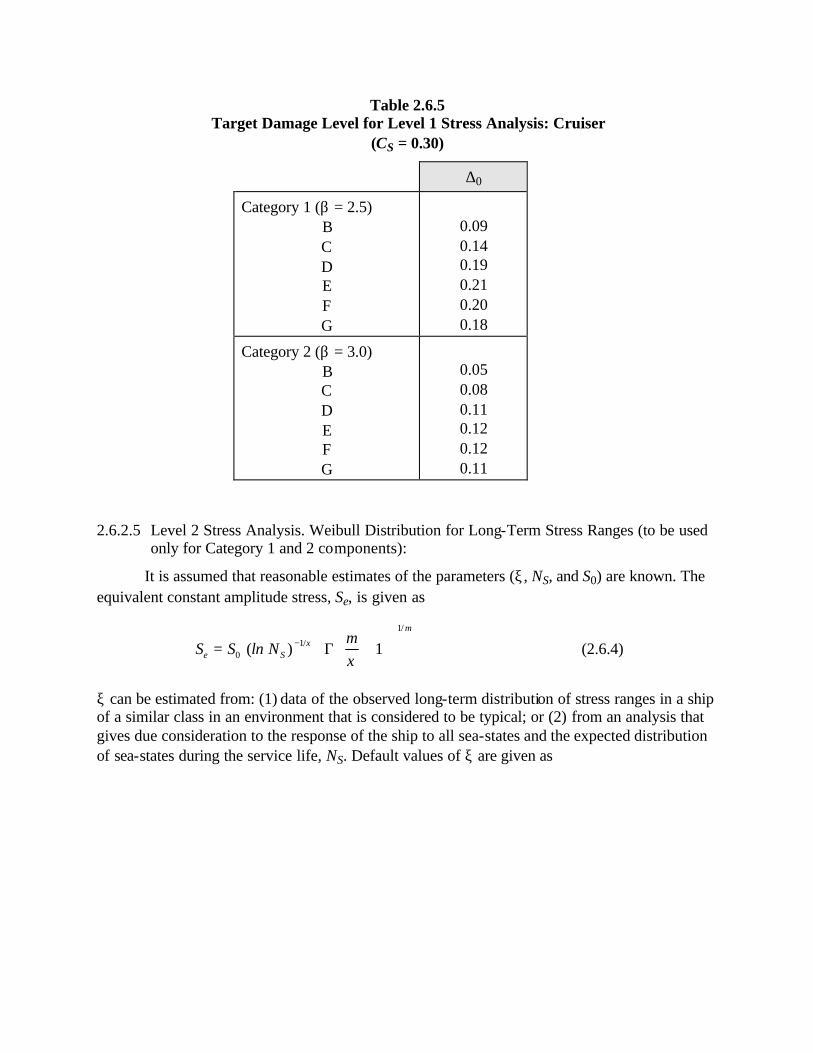
Table 2.6.5 Target Damage Level for Level 1 Stress Analysis: Cruiser
(CS = 0.30)
∆0
Category 1 (β = 2.5) B C D E F G
0.09 0.14 0.19 0.21 0.20 0.18
Category 2 (β = 3.0) B C D E F G
0.05 0.08 0.11 0.12 0.12 0.11
2.6.2.5 Level 2 Stress Analysis. Weibull Distribution for Long-Term Stress Ranges (to be used only for Category 1 and 2 components):
It is assumed that reasonable estimates of the parameters (ξ, NS, and S0) are known. The equivalent constant amplitude stress, Se, is given as
S S ln Nm
e S
m
= +
−0
1
1
1( ) /
/
ξ
ξΓ (2.6.4)
ξ can be estimated from: (1) data of the observed long-term distribution of stress ranges in a ship of a similar class in an environment that is considered to be typical; or (2) from an analysis that gives due consideration to the response of the ship to all sea-states and the expected distribution of sea-states during the service life, NS. Default values of ξ are given as

Table 2.6.5a Default Values of the Weibull Shape Parameter, ξ
ξ TANKER CRUISER
Exposure to normal operational seas 1.0 1.2
Exposure to extreme environments, e.g., North Atlantic, TAPS, or where significant dynamic response is anticipated
1.2
1.4
Fagitue damage is computed using Eq. (2.6.1). Values of the target damage level are given in Table 2.6.6 for the tanker and Table 2.6.7 for the cruiser.
Table 2.6.6 Target Damage Level for Level 2 Stress Analysis: Tanker
(CS = 0.25)
∆0
Category 1 (β0 = 2.0) B C D E F G
0.25 0.33 0.41 0.45 0.42 0.38
Category 2 (β0 = 2.5) B C D E F G
0.14 0.20 0.26 0.27 0.26 0.24

Table 2.6.7 Target Damage Level for Level 2 Stress Analysis: Cruiser
(CS = 0.25)
∆0
Category 1 (β0 = 2.5) B C D E F G
0.14 0.20 0.26 0.27 0.26 0.24
Category 2 (β0 = 3.0) B C D E F G
0.08 0.12 0.16 0.17 0.16 0.16
2.6.2.6 Level 3 Stress Analysis. Histogram of the Long-Term Distribution of Stress Ranges:
The histogram will consist of a table of values of constant amplitude stress ranges, Si, and the associated number of cycles, Ni, i = 1,J, where J is the number of levels chosen. The histogram is constructed from: (1) data of the observed long-term distribution of stress ranges in a ship of a similar class in an environment that is cons idered to be typical; or (2) from an analysis that gives due consideration to the response of the ship to all sea-states and the expected distribution of sea-states during the service life, NS.
The equivalent constant amplitude stress, Se, is given as,
SN
N SeS
i im
i
Jm
=
=∑1
1
1/
(2.6.5)
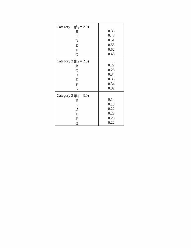
Fatigue damage is computed using Eq. (2.6.1). Values of the target damage level are given in Table 2.6.8 for the tanker and Table 2.6.9 for the cruiser.
Table 2.6.8 Target Damage Level for Level 3 Stress Analysis: Tanker
(CS = 0.20)
∆0
Category 1 (β0 = 2.0) B C D E F G
0.35 0.43 0.51 0.55 0.52 0.48
Category 2 (β0 = 2.5) B C D E F G
0.22 0.28 0.34 0.35 0.34 0.32
Category 3 (β0 = 3.0) B C D E F G
0.14 0.18 0.22 0.23 0.23 0.22

Table 2.6.9 Target Damage Level for Level 3 Stress Analysis: Cruiser
(CS = 0.20)
∆0
Category 1 (β0 = 2.5) B C D E F G
0.22 0.28 0.34 0.35 0.34 0.32
Category 2 (β0 = 3.0) B C D E F G
0.14 0.18 0.22 0.23 0.23 0.22
Category 3 (β0 = 3.5) B C D E F G
0.08 0.11 0.15 0.15 0.15 0.15
2.6.2.7 Level 4 Stress Analysis. Sea-States Modeled as Stationary Gaussian Processes:
It is anticipated that this method be analytical, although the collection and use of data is encouraged.
The distribution of operational sea-states in the service life of the ship is defined. The sea-states are discretized into J levels. The number of cycles for each level, Ni, is recorded. For each sea-state, the significant wave height, HSi, and/or the root mean square (RMS) wave height σXi, is determined; this value is translated into the RMS nominal stress, σi at the detail under consideration.
The equivalent constant amplitude stress, Se, is
Sm f
fei i i
m m
= +
2 83
21
0
1
./
ΓΣψ σ
(2.6.6)

where ψ i = the fraction of time in the ith sea-state, fi = the frequency of wave loading in the ith sea-state, f0 is the average frequency of the stress cycles over the service life, and σi = the RMS of the stress process in the ith sea-state.
Fatigue damage is computed using Eq. (2.6.1). Values of the target damage level are given in Table 2.6.10 for the tanker and Table 2.6.11 for the cruiser.
Table 2.6.10 Target Damage Level for Level 4 Stress Analysis: Tanker
(CS = 0.15)
∆0
Category 1 (β0 = 2.0) B C D E F G
0.48 0.56 0.62 0.66 0.63 0.59
Category 2 (β0 = 2.5) B C D E F G
0.32 0.38 0.43 0.44 0.44 0.42
Category 3 (β0 = 3.0) B C D E F G
0.22 0.26 0.30 0.30 0.30 0.30

Table 2.6.11 Target Damage Level for Level 4 Stress Analysis: Cruiser
(CS = 0.15)
∆0
Category 1 (β0 = 2.5) B C D E F G
0.32 0.38 0.43 0.44 0.44 0.42
Category 2 (β0 = 3.0) B C D E F G
0.22 0.26 0.30 0.30 0.30 0.30
Category 3 (β0 = 3.5) B C D E F G
0.15 0.18 0.21 0.20 0.20 0.21

APPENDIX A LITERATURE REVIEW: STRUCTURAL RELIABILITY AND CODE DEVELOPMENT
A.1 General Background
The modern era of probabilistic structural design started after the Second World War. In 1947, a paper entitled, “The Safety of Structures,” appeared in the Transactions of the American Society of Civil Engineers. This historical paper, written by A.M. Freudenthal, suggested that rational methods of developing safety factors for engineering structures should give due consideration to observed statistical distributions of the design factors. It wasn’t until the 1960’s that there was rapid growth of academic interest in structural reliability theory, stimulated in part by the publication of another paper by Freudenthal [Freudenthal, Garrelts, and Shinozuka (1966)].
In light of the practical difficulties in employing a probabilistic-statistical approach to design criteria development, C.A. Cornell (1969) suggested the use of a second moment format, and introduced the concept of a safety index. The safety index was the probabilistic analog of the factor of safety, widely employed to account for uncertainties in the design process. The method of computing the safety index is called mean value first order second moment analysis (MVFOSM).
But Cornell’s safety index depended on how the failure, or limit state, equation was written. This lack of invariance problem was resolved by Hasofer and Lind (1974) in a landmark paper in structural reliability. Their concept of a generalized safety index has been employed in all subsequent contributions to computational reliability.
But the Hasofer-Lind method used only the mean and standard deviation for each of the design variables. To account for full distributional information, a transformation of the basic variables to standard normal variates can be made [Rosenblatt (1952), Paloheimo and Hannus (1974), and Hohenbichler and Rackwitz (1981)]. Then beta (the safety index) would be computed using the Hasofer-Lind algorithm. Such an approach is now called a first order reliability method (FORM). A popular numerical method for computing beta is the Rackwitz-Fiessler algorithm [Rackwitz and Fiessler (1978)].
The probability of failure using FORM can be estimated by evaluating the standard normal distribution function at minus beta. Because significant errors were observed in some FORM analyses, more advanced “second order” reliability methods were developed [Breitung (1984), Wu and Wirsching (1984), and Tvedt (1983)]. These methods provide accurate estimates of the probability of failure in those cases where the limit state is generally well behaved.
A.2 Structural Reliability for Ships
In the almost two decades since researchers first began to look at the desirability of using probabilistic methods in the structural design of ships [Mansour (1972a, 1972b), Mansour and Faulkner (1972)], a significant amount has been accomplished. (Please refer to list of references). Much of that effort has been sponsored by the Ship Structure Committee through its projects and through interaction with various other governmental agencies and international organizations (e.g., ISSC). Because design is a synthesis process which involves configuration, analysis, assessment, and reconfiguration, early probabilistic efforts were aimed at developing the reliability assessment tools [Ang (1973), Ang and Cornell (1974), Stiansen et al. (1979), Ayyub

and Haldar (1984), White and Ayyub (1985)]. While some work continues in this area, it is generally felt that there are sufficient means available today to allow for the accurate assessment of the structural reliability components. There is still a continuing effort, which is looking at how these methods and procedures can be used in a system analysis.
The earliest applications of reliability methods to ship structures focused on overall hull girder reliability when subjected to wave bending moments [Mansour (1974), Stiansen et al. (1979), Mansour, et al. (1984), White and Ayyub (1985)]. This was a natural outgrowth of the way in which ship structures were designed. The wave bending response of the ships’ hull was seen as the mode in which failure would be catastrophic. It had been one of the biggest concerns to ship designers for over 100 years. But as reliability assessments of hull strength began to be performed, it was found that some other modes are just as important. Of particular concern has been the ultimate strength of the orthogonally-stiffened panels that make up the deck and bottom of a ship. Because of the very large in-plane loads and the possibility of large lateral pressures, the reliability of these panels is of concern. Failure of one of these panels could lead to progressive collapse and ultimate hull girder failure. Recent work in applying reliability methods to the ultimate strength of gross panels using second moment methods [Nikolaidis, et al. (1993)] has shown considerable promise.
Within the marine industry, the focus of the efforts in reliability-based design fell on three specific areas: loadings from the seaway, fatigue of structural details, and hull girder strength modeling. The loadings area has seen a tremendous amount of effort in attempts to develop statistical models for each of the major load effects [e.g., Guedes Soares and Moan (1985, 1988), Guedes Soares (1984), Ochi (1978, 1979a, 1979b, 1981), Sikora et al. (1983), Mansour (1987)]. The Ship Structures Committee recently sponsored work on investigating the uncertainties associated with loads and load effects [Nikolaidis and Kaplan (1991)], and on loads and load combinations [Mansour and Thayamballi (1993)].
A.3 Probability-Based Codes
There has been considerable interest within the offshore industry in developing a reliability-based design procedure. The American Petroleum Institute was one of the early leaders in this effort, sponsoring a number of research efforts which culminated in the proposed revision to the API design-recommended practice for fixed offshore structures [API RP2A-LRFD, Moses (1985, 1986)]. Other researchers have looked into a variety of approaches for including reliability methods in fatigue design [Munse, et al. (1983), Wirsching (1984), Wirsching and Chen (1988), Wirsching, et al. (1991), Madsen, et al. (1986), White and Ayyub (1987b), Kihl (1993)].
Mansour, et al. (1984), White and Ayyub (1987a), and Mansour et al. (1993), in SR-1330, provided a demonstration for computing the partial safety factors in a reliability-based design code for marine structures. Guedes Soares and Moan (1985) demonstrated how to develop checking equations for the midship section under longitudinal bending. They took into account uncertainties in stillwater and wave bending moments in calibrating the load and strength factors. Committee V.2 of ISSC also presented an example of calibrating load and strength factors for the structural design of ship hulls.
Reliability-based design codes were developed by the American Concrete Institute (ACI) using MVFOSM, and by the American Institute of Steel Construction [AISC (1994)], who used a concept, based on the lognormal format, called Load and Resistance Factor Design (LRFD)

[Galambos and Ravindra (1978), plus seven other papers in the same journal]. An effort was made by the National Standards Institute (ANSI) to develop probability-based load criteria for buildings [Ellingwood et al. (1982a, 1982b)]. This work is now published as ASCE 7-93 [ASCE (1993)]. Later, in an effort directed by Fred Moses, the American Petroleum Institute (API) extrapolated LRFD technology for use in fixed offshore platforms [API (1989)]. Other efforts which provide excellent and comprehensive summaries of implementation of modern probabilistic design theory into design codes include those of Siu, Parimi, and Lind (1975) for the National Building Code of Canada, Ellingwood et al. (1980) for the National Bureau of Standards, and the CIRIA 63 (1977) report.

APPENDIX B TARGET RELIABILITIES
B.1 Target Values
To establish probability-based design criteria, it is necessary to define a maximum allowable risk (or probability of failure), p0. Define
p0 = target risk, or probability of failure
pf = the probability of failure (as estimated from analyses)
Then, for a safe design,
pf ≤ p0 (B.1)
Alternatively, the safety index can be used. In fact, its use is more common for design criteria development. Define
β0 = target safety index β = safety index (as estimated from analyses)
β0 = Φ-1(p0) β = Φ-1(pf) (B.2)
Φ is the standard normal cumulative distribution function (cdf). Then, for a safe design,
β ≥ β0 (B.3)
The selection of target reliabilities is a difficult task (Payer, et al., 1994). These values are not readily available and need to be generated or selected. Also, these levels might vary from one industry to another due to factors such as the implied reliability levels in currently used design practices by industries, failure consequences, public and media sensitivity, or response to failures that can depend on the industry type, types of users or owners, design life of a structure, and other political, economic, and societal factors.
B.2 Method of Selecting Target Values
Target reliability values will be chosen by the authors of this report. The process by which they will do this is described in the following.
What value should be chosen for the target reliability (or target safety index)? In general, there are no easy answers. There are three methods which have been employed:
(1) The code writers and/or the profession agrees upon a “reasonable” value. This method is used for novel structures where there is no prior history.
(2) Code calibration. (calibrated reliability levels that are implied in currently used codes) The level of risk is estimated for each provision of a successful code. Safety margins are adjusted to eliminate inconsistencies in the requirements. This method has been commonly used for code revisions.
(3) Economic value analysis. (cost benefit analysis) Target reliabilities are chosen to minimize total expected costs over the service life of the structure. In theory, this

would be the preferred method, but it is impractical because of the data requirements for the model.
The second approach was commonly used to develop reliability-based codified design such as the LRFD format. The target reliability levels, according to this approach, are based on calibrated values of implied levels in a currently used design practice. The argument behind this approach is that a code represents a documentation of an accepted practice. Therefore, since it is accepted, it can be used as a launching point for code revision and calibration. Any adjustments in the implied levels should be for the purpose of creating consistency in reliability among the resulting designs according to the reliability-based code. Using the same argument, it can be concluded that target reliability levels used in one industry might not be fully applicable to another industry.
The third approach is based on cost-benefit analysis. This approach was used effectively in dealing with designs for which failures result in only economic losses and consequences. Because structural failures might result in human injury or loss, this method might be very difficult to use because of its need for assigning a monetary value to human life. Although this method is logical on an economic basis, a major shortcoming is its need to measure the value of human life. Consequently, the second approach is favored for this study and is discussed further in the following sections.
An important consideration in the choice of design criteria is the consequences of failure. Clearly the target reliability relative to collapse of the hull girder should be larger than that of a non-critical welded detail relative to fatigue.
In this exercise, a combination of (1) and (2) will be used. The following section provides a summary of the sources of information that will be used to make decisions on target reliabilities for the structural systems and subsystems considered.
B.3 Calibrated Reliability Levels
A number of efforts, in which target reliability levels (i.e., safety indices or β values) were developed for the purpose of calibrating a new generation structural design code to an existing code, have been completed.
According to Structural Reliability: Analysis and Prediction [Melchers (1987)], the general methodology for code calibration based on specific reliability theories, using second-moment reliability concepts, is discussed by Allen (1975), Baker (1976), CIRIA (1977), Hawrenek and Rackwitz (1976), Guiffre and Pinto (1976), Ravindra and Galambos (1978), Ellingwood et al. (1980), Lind (1976), and Ravindra et al. (1969). The key steps in the process, following the discussion in Melchers (1987), are as follows. First, the scope of the design situation must be identified (e.g., material, loads, structural type) and narrowed to fit the specific situation. Next, a design space reflecting all key variables (nominal yield stresses, range of applied loads, continuity conditions, etc.) is chosen and divided into discrete zones. These zones are used to develop typical designs using existing codes. Next, performance functions for the failure modes, expressed in terms of the basic variables, are defined. The statistical properties (distributions, means, variances, and average-point- in-time values) of the basic variables are used for the determination of the β indices using a specified method for reliability analysis (e.g., moment methods).

Next, each of the designs obtained above, together with the performance functions and the statistical data derived above, are used to determine β for each zone. Repeated analyses will yield the variation of β . From these data, a wieghted β is obtained and used as a target reliability level β0. Melchers notes that frequently the information is insufficient for this determination and one must make a “semi- intuitive” judgment in selecting β0 values; for example, recognizing a value is used for dead, live, and snow load combinations as compared to dead, live, and wind load combinations or dead, live, and earthquake load combinations. Divergent β0 values should be corrected by means of the partial factor(s) on material strength or resistance (e.g., through the strength reduction factor).
B.4 Sources of Information Used to Establish Target Reliabilities
B.4.1 SSC Project SR-1344
Project SR-1344 (Mansour Engineering, Inc., Contractor) is entitled “Assessment of Reliability of Existing Ship Structures.” The goal of this program is to estimate the level of risk relative to several failure modes in ship structure and structural components for four ships: two cruisers, a tanker, and a containership. One of the purposes of this project is to provide some guidance regarding reliabilities implied by the existing traditional design code requirements. In the forum to select probability-based design criteria, the principal testimony will be provided by these values.
Preliminary results from SR-1344 are summarized in Table B.1. At this time, the safety indices listed must be considered to be the first estimates.
B.4.2 Studies by A.E. Mansour
Mansour (1974) performed a preliminary study of the safety index relative to the ultimate strength of the hull girder over the service life for tankers, cargo ships, and bulk carriers. The results are plotted in Figs. B.1 and B.2 for the initial yield failure mode.
Table B.1 Preliminary Results of SR-1344 All mean values in 105 long ton-ft
STILLWATER WAVE STRENGTH SAFETY Mean COV Mean COV Mean COV INDEX, β hog(a) (%) hog sag(b) (%) hog sag (%) hog sag
Cruiser #1 0.72 15 1.69 2.59 9 5.23 5.18 10 5.51 5.46 Cruiser #2 0.58 15 1.56 2.78 9 4.38 4.55 10 5.23 4.46
Tanker 2.53 25 5.86 7.14 9 11.2 10.5 12 2.54 4.04 SL-7 3.27 25 9.70 13.8 9 18.9 22.9 12 2.98 4.20
DISTRIBUTION NORMAL EVD NORMAL
NOTES: (a) Worst case only considered

(b) Includes a slamming factor of 1.3 for Cruiser #1, Cruiser #2, and SL-7; and a factor of 1.2 for the tanker
B.4.3 LRFD Requirements
In the code calibration process of Load and Resistance Factor Design, Galambos and Ravindra (1978) recommended a default value of β0 = 3.0 as a general requirement. It is assumed by the authors that this would be for a component of a highly redundant structure. It should not apply if the consequences of failure are serious.
Reed and Brown (1992) provide a summary of the target reliability levels used in the AISC LRFD specifications. In addition to the values provided in Tables B.2 and Table B.3, values for high strength bolts in tension and shear were given as 5.0 to 5.1, and 5.9 to 6.0, respectively. Also, a value for fillet welds of 4.4 is given. Detailed information about these values are provided by Galambos (1989).
B.4.4 ANS (American National Standard) A58
While the specific reliabilities will be a function of the strength criteria needed for specific materials and load combinations within designated structures, it is useful to have an indication of the range of possible target reliability levels. Ellingwood et al. (1980) present ranges for reliability levels for metal structures, reinforced and prestressed concrete structures, heavy timber structures, and masonry structures, as well as discussions of issues that should be considered when making the calibrations. Table B.2 provides typical values for target reliability levels. This table was developed based on values provided by Ellingwood et al. (1980). The target reliability levels shown in Table B.3 were also used by Ellingwood and Galambos (1982) to demonstrate the development of partial safety factors. The β0 values in Tables B.2 and B.3 are for structural members designed for 50 years of service.


Table B.2 Target Reliability Levels
Structural Type Target Reliability Level (β0) Metal structures for buildings (dead, live, and snow loads)
3
Metal structures for buildings (dead, live, and wind loads)
2.5
Metal structures for buildings (dead, live, and snow, and earthquake loads)
1.75
Metal connections for buildings (dead, live, and snow loads)
4 to 4.5
Reinforced concrete for buildings (dead, live, and snow loads) ⋅ductile failure ⋅brittle failure
3
3.5
Table B.3 Target Reliability Levels Used by Ellingwood and Galambos (1982)
Member, Limit State Target Reliability Level (β0) Structural Steel Tension member, yield Beams in flexure Column, intermediate slenderness
3.0 3.0 3.5
Reinforced Concrete Beam in flexure Beam in shear Tied column, compressive failure
3.0 3.0 3.5
Masonry, unreinforced Wall in compression, uninspected Wall in compression, uninspected
5.0 7.5

B.4.5 Canadian Standard Association (CSA) Deliberations
The following figures were presented for review for possible adoption by the CSA for design criteria for offshore installations in Canadian waters.
10-5/year Safety Class 1. Failure results in a great loss of life or a high potential for environmental damage.
10-3/year Safety Class 2. Failure would result in small risk to life and a low potential for environmental damage.
B.4.6 National Building Code of Canada
Madsen et al. (1986) discuss target reliability levels that were used by the National Building Code of Canada (1977) for hot-rolled steel structures. The target reliability values were selected as follows: β0 = 4.00 for yielding in tension and flexure, β0 = 4.75 for compression and buckling failure, and β0 = 4.25 for shear failures. These values are larger than the values in Tables B.2 and B.3 because they reflect different environmental loading conditions and possibly different design life.
B.4.7 A.S. Veritas Research
A.S. Veritas Research was a subsidiary of Det norske Veritas. Target annual probabilities, recommended by this agency, are given in Table B.4 [see also Lotsberg (1991)]. Note that these values are annual probabilities. Thus, for example, if the failure is Type 1 (ductile failure with reserve capacity) and Serious, then the annual target is p1 = 10-4. But if the service life is 20 years, then the target for the service life would be p0 = 20 (10-4) or 2⋅10-3.
B.4.8 Nordic Building Committee
Madsen et al. (1986) also discuss target reliability levels that were used by the Nordic Building Code Committee (1978). The target reliability values were selected depending on the failure consequences of a building in the following ranges: β0 = 3.1 for less serious failure consequences, β0 = 5.2 for very serious failure consequences, and β0 = 4.27 for common cases.
B.4.9 AASHTO Specifications
Moses and Verma (1987) suggested target reliability levels in calibrating bridge codes (i.e., AASHTO Specifications). Assuming that bridge spans of less than 100 ft. are most common, a β0 of 2.5 to 2.7 is suggested for redundant bridges, and a β0 of 3.5 for non-redundant bridges.
Table B.4 Veritas Target Failure Probabilities
Ref: A.S. Veritas Research (Report No. 91-2000); Norwegian agency that certifies large scale structures worldwide

Target (annual) failure probabilities (Target safety index in parentheses)
Failure Type
Failure Consequences
1 2 3
Not serious 10-3 (3.09) 10-4 (3.71) 10-5 (4.26)
Serious 10-4 (3.71) 10-5 (4.26) 10-6 (4.75)
Very serious 10-5 (4.26) 10-6 (4.75) 10-7 (5.20)
FAILURE TYPE:
1. Ductile failure with reserve strength capacity resulting from strain hardening.
2. Ductile failure with no reserve capacity.
3. Brittle fracture and instability
FAILURE CONSEQUENCES:
Not serious . A failure implying small possibility for personal injuries; the possibility for pollution is small and the economic consequences are considered to be small.
Serious . A failure implying possibilities for personal injuries/fatalities or pollution or significant economic consequences.
Very serious . A failure implying large possibilities for several personal injuries/fatalities or significant pollution or very large economic consequences.
B.4.10 API Fatigue Studies
Using the best data available at the time, Wirsching (1984) estimated the safety index as β0 ≈ 2.5 implied by the API RP2A (for fixed offshore structures) fatigue design guidelines in tubular welded joints. The reality is that the reference wave designs most members (at least for platforms in water depths less than 300 feet), so that few joints have a safety index that low.
B.5 Recommended Target Safety Indices
Recommended target safety indices are summarized in Table B.5. These are lifetime values that are used to derive partial safety factors in this prototype code. The values were based on professional judgment applied to the evidence presented above in Section B.4.

Table B.5 Recommended Target Safety Indices
Relative to Service Life of Ships
Tanker, β0 Cruiser, β0
Hull girder collapse Hull girder initial yield Unstiffened panel Stiffened panel Fatigue Category 1 (Not Serious) Category 2 (Serious) Category 3 (Very Serious)
4
4.5 3
3.5
2.0
2.5
3.0
5
5.5
3.5 4
2.5
3.0
3.5

APPENDIX C PARTIAL SAFETY FACTORS (PSF) AND SAFETY CHECK EXPRESSIONS
C.1 Traditional Safety Check Expression
A design expression involves stress S (load, force, moment, pressure, etc.) and strength R (the minimum stress tha t causes failure in the component). In general, both S and R possess significant uncertainty. This uncertainty can be quantified by a statistical distribution, i.e., a random variable. Failure occurs when S exceeds R. Because both are random variables, the probability of (S > R) can be computed. This probability is called the estimated probability of failure.
The general goal of design is to select the geometry of a component, balancing both investment cost with the expected cost of failure. Thus, the goal of a design code containing safety check expressions is to provide cost-efficient, reliable designs. Probabilistic design theory provides a mechanism for providing a high quality design code that ensures a high level of structural integrity, avoiding costly inconsistencies and needless investment costs.
While conventional (traditional) design code safety check expressions may vary in format, they are essentially of the same form,
SRFSn
n< (C.1)
for a safe design. Sn is nominal value of stress. It is a value on the safe (or right) side of the distribution of S, although sometimes it is the best estimate of S. Rn is nominal strength, and is usually a value on the safe or left side of the distribution of R although it also could be a mean or median value. Additional uncertainty is accounted for by the factor of safety FS, where FS > 1. Historically, FS, Sn, and Rn are defined by committees charged with writing the code. These values are typically experienced-based.
In summary, structural integrity in the face of significant uncertainties is maintained by proper choice of FS, Sn, and Rn. Note that no meaningful index of quality or reliability can be explicitly implied from these values.
In American design practice, the factor of safety is generally applied to the strength, as shown in Eq. (C.1). The right-hand side can be interpreted as the maximum allowable stress, and the use of Eq. (C.1) is frequently referred to in the literature as allowable stress design (ASD) or working stress design (WSD).
While traditional ASD and WSD have served the engineering profession well, it has been suggested that the design codes lack consistency. Some provisions of the code produce over-designs, some produce under-designs. There has been a suspicion that this inconsistency results in a serious economic penalty. Starting from Freudenthal (1947), it has been argued in many papers that the use of probabilistic-statistical methods, giving explicit consideration of the statistical distribution of each, has the promise of producing better engineered designs. And, indeed, many organizations and agencies worldwide have already implemented probability-based design codes and have demonstrated significant cost savings.

C.2 Options for Probability-Based Safety Check Expressions
Options for the development of safety check expressions using probabilistic methods and reliability technology include the following:
(1) Specify the maximum allowable probability of failure. The designer would be required to perform a probabilistic analysis of the component or system. Subjective judgments would have to be made on the quality of data sets and distributional models of the random design factors. Generally, this is not a practical option for general design.
(2) Specifying a minimum allowable safety index. Again, the designer would perform a reliability analysis. A safety index can be computed using only the mean and standard deviation of the design factors.
(3) Using a partial safety factor format. Among code writers, this seems to be the method of choice. A target safety index is translated into safety factors applied separately to the key stress and strength variables.
(4) Using a working or allowable stress format. There is only one safety factor (e.g., Eq. (C.1)), and this factor can have a probability basis. But there are real advantages in using the partial safety factor format.
Upon review of the options, it was decided that the partial safety factor format provided the best compromise. The partial safety factors are derived from full distributional information from all of the design factors, and the format of the safety check equations are similar to those used by designers in traditional codes.
C.3 The Generalized Safety Index and First Order Reliability Analysis
Partial safety factors can be derived using first order (FORM) or second order (SORM) reliability methods, mathematical processes for computing point probabilities. These methods, described in Hasofer and Lind (1974), Madsen et al. (1986), and Melchers (1987), are summarized here for reference.
Hasofer-Lind (H-L) Generalized Safety Index. Define the design factors in a failure equation for a structural component,
X = X1, X2, ⋅⋅⋅, Xk (C.2)
In general, each Xi will be a random variable having a known mean µ and standard deviation, σ. Define the limit state function g(X) so that,
g(X) < 0 → FAILURE (C.3)
The limit state is defined as
g(X) = 0
This is the boundary between the safe and the failed regions in design parameter space.
Define reduced variables as,

uX
ii i
i
=− µ
σ i = 1,k (C.4)
Then the limit state equation can be expressed in terms of the reduced variables,
g′(u) = 0 (C.5)
Define the generalized safety index (beta) as the minimum distance from the origin of the reduced coordinates in design parameter space to the limit state function in reduced coordinates. Beta is illustrated for the case of two variables in Fig. C.1.
In the special case where g is a linear function of X and all Xi have normal distributions, then the probability of failure will be,
pf = Φ(-β) (C.6)
where Φ is the standard normal cumulative distribution function.
The point u* in Fig. C.1 is called the “design point” or the “most probable failure point.” It is the point on the limit state which is most probable. The most probable point plays a key role in deriving the partial safety factors. In terms of the basic variables, X i
* will be a value in the right tail distribution of a stress variable and in the left tail distribution of a strength variable. A stress variable is one in which the design becomes dangerous if the value becomes too large, and a strength variable is one in which the design is dangerous if the value becomes too small. Recall that the design point has the same basic characteristic that the nominal values of Eq. (C.1) had.
First Order Reliability Method. Distributional information on each Xi, even if it were available, is not used in the Hasofer-Lind generalized safety index. But in an extension of the H-L method, FORM requires that the distribution of each Xi be specified.
Transform all variables to standard normal variates, u, using the condition that, for each variable,
FX(x) = Φ(u) (C.7)

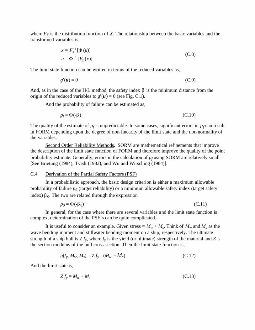
where FX is the distribution function of X. The relationship between the basic variables and the transformed variables is,
x F u
u F xX
X
=
=
−
−
1
1
[ ( )]
[ ( )]
Φ
Φ (C.8)
The limit state function can be written in terms of the reduced variables as,
g′(u) = 0 (C.9)
And, as in the case of the H-L method, the safety index β is the minimum distance from the origin of the reduced variables to g′(u) = 0 (see Fig. C.1).
And the probability of failure can be estimated as,
pf = Φ(-β) (C.10)
The quality of the estimate of pf is unpredictable. In some cases, significant errors in pf can result in FORM depending upon the degree of non- linearity of the limit state and the non-normality of the variables.
Second Order Reliability Methods. SORM are mathematical refinements that improve the description of the limit state function of FORM and therefore improve the quality of the point probability estimate. Generally, errors in the calculation of pf using SORM are relatively small [See Brietung (1984), Tvedt (1983), and Wu and Wirsching (1984)].
C.4 Derivation of the Partial Safety Factors (PSF)
In a probabilistic approach, the basic design criterion is either a maximum allowable probability of failure p0 (target reliability) or a minimum allowable safety index (target safety index) β0. The two are related through the expression
p0 = Φ(-β0) (C.11)
In general, for the case where there are several variables and the limit state function is complex, determination of the PSF’s can be quite complicated.
It is useful to consider an example. Given stress = Mw + Ms. Think of Mw and Ms as the wave bending moment and stillwater bending moment on a ship, respectively. The ultimate strength of a ship hull is Z fy, where fy is the yield (or ultimate) strength of the material and Z is the section modulus of the hull cross-section. Then the limit state function is,
g(fy, Mw, Ms) = Z fy - (Mw +Ms) (C.12)
And the limit state is,
Z fy = Mw + Ms (C.13)
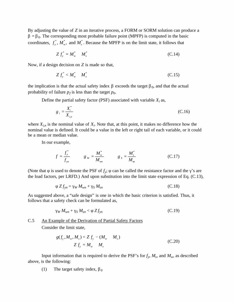
By adjusting the value of Z in an iterative process, a FORM or SORM solution can produce a β = β0. The corresponding most probable failure point (MPFP) is computed in the basic coordinates, f M My w s
* * *, , and . Because the MPFP is on the limit state, it follows that
Z f M My w s* * *= + (C.14)
Now, if a design decision on Z is made so that,
Z f M My w s* * *< + (C.15)
the implication is that the actual safety index β exceeds the target β0, and that the actual probability of failure pf is less than the target p0.
Define the partial safety factor (PSF) associated with variable Xi as,
γ ii
i n
XX
=*
,
(C.16)
where Xi,n is the nominal value of Xi. Note that, at this point, it makes no difference how the nominal value is defined. It could be a value in the left or right tail of each variable, or it could be a mean or median value.
In our example,
φ γ γ= = =f
fMM
MM
y
ynW
w
wnS
s
sn
* * *
(C.17)
(Note that φ is used to denote the PSF of fy; φ can be called the resistance factor and the γ’s are the load factors, per LRFD.) And upon substitution into the limit state expression of Eq. (C.13),
φ Z fyn = γW Mwn + γS Msn (C.18)
As suggested above, a “safe design” is one in which the basic criterion is satisfied. Thus, it follows that a safety check can be formulated as,
γW Mwn + γS Msn < φ Z fyn (C.19)
C.5 An Example of the Derivation of Partial Safety Factors Consider the limit state,
g f M M Z f M M
Z f M My w s y w s
y w s
( , , ) ( )= − +
= + (C.20)
Input information that is required to derive the PSF’s for fy, Ms, and Mw, as described above, is the following:
(1) The target safety index, β0

(2) The distribution family of fy, e.g., Weibull
(3) The COV of fy, CR
(4) The distribution of Mw
(5) The COV of Mw, CW
(6) The distribution family of Ms
(7) The COV of Ms, CS
(8) The ratio of the mean loads, µW/µS
(9) Definition of the nominal value of fy
(10) Definition of the nominal value of Mw
(11) Definition of the nominal value of Ms
In this example, the input information is provided in Table C.1.
Note that Z was introduced in this problem as the cross-sectional area (or perhaps section modulus). But it can also be thought of as a scale factor for the mean of fy.
The partial safety factors will be a function of the ratio of the means, µW/µS. But for a given µW/µS, the mean of fy does not have to be specified as it is scaled by Z.
In order to run the reliability program, specific values must be input. First, it is assumed that µW/µS = 1. The values chosen are µR = µW = µS = 1. Because the mean values are also the nominal values, when the reliability program (e.g., CALREL, FPI) is run, the MPFP values and the PSF’s are identical (Eq. (C.17)).
Table C.1 Input Data for Determination
of Partial Safety Factors
Distribution
Nominal Value
COV
fy Weibull µR 0.10
Mw
EVD (Type 1 extreme value distribution of
maxima)
µW
0.20
Ms Normal µS 0.20

µW/µS 1.0
Target Safety Index, β0 3.0
A computer code (e.g., CALREL, FPI) is used to perform the reliability analysis. Here, the two types of analysis as described above are performed: (1) first order reliability analysis (FORM), and (2) second order reliability analysis (SORM). For each of these methods, the computer code is run with different values of A until the computed β = β0. The resulting MPFP (and, therefore, the partial safety factors) of each of the design variables is given in Table C.2.
Table C.2 Partial Safety Factors
[also equal to the MPFP for this example]
φ γW γS
FORM* 0.677 1.26 1.18
SORM 0.660 1.25 1.18
*The value of Z, for this example, was 3.60

It has been observed from a number of examples that the FORM and SORM solutions are very close. Because the FORM solution process is generally more robust (fewer numerical difficulties), FORM analysis was used to derive the PSF’s of this study. Using the FORM results, the safety check expression would be,
1.25 Mwn + 1.18 Msn < 0.660 Z fyn (C.21)
Note that the PSF’s given in Eq. (C.21) are only for the case of µW/µS = 1.0. In general, the PSF’s will be functions of this ratio.
C.6 More Complicated Forms of the Limit State Function
The direct approach. Consider a limit state of the form,
Z aXbY
M Mw s2 +
= +
where X, Y, Mw, and Ms are random variables, and a and b are constants. Again, Z can play the role of a scale factor. Here, the resistance variable (left-hand side) is a function of several design factors.
Given the distributions of the four random variables, the PSF’s for each variable can be computed using an advanced reliability program, as described in the above examples. Each PSF will be a function of four parameters: µW/µS, µX/µS, a/µS, and a/b.
The safety check will be of the form,
a Xb
YM MX n
Y nW wn S sn( )γ
γγ γ2 + = +
An alternative approach. In this approach, there will be one PSF for resistance. Let
f aXbYy = +2
The mean ratios that define fy are µX/µY, a/µX, and a/b.
The magnitude of µX and µY is scaled by Z. Given the three mean ratios, and making an arbitrary choice of µX = 1, the distribution of X and Y are defined. Using Monte Carlo simulation, obtain a random sample of fy. Fit a standard distribution to fy. Then use FORM to compute φ. The safety check expression will be
φ γ γaXbY
M Mnn
W wn S sn2 +
= +
Each of the PSF’s will be functions of the µW/µS, µX/µS, a/µS, and a/b.

APPENDIX D COMMENTARY: LIMIT STATE FUNCTIONS FOR HULL GIRDER COLLAPSE
D.1 Discussion: Hull Capacity
The determination of the collapse load, which defines the true ultimate strength of a ships’ girder, has become a topic of increased interest to the ship research and design communities. One of the reasons behind this interest is that knowledge of the limiting conditions beyond which a hull girder will fail to perform its function will, undoubtedly, help in assessing more accurately the true margin of safety between the ultimate capacity of the hull and the maximum combined moment acting on the ship. Assessing the margins of safety more accurately will lead to a consistent measure of safety which can form a fair and a good basis for comparisons of ships of different sizes and types. It may also lead to changes in regulations and design requirements with the objective of achieving uniform safety standards among different ships.
The state-of-the-art in determining the true ultimate strength of a ship girder is at the point where changes in design standards can be made. Various definitions of the ultimate strength of a hull have been proposed, but the most acceptable one is the recommendation reported by Committee 10 in the proceedings of the Third International Ship Structures Congress, Vol. 2, 1967, quoted as:
“This occurs when a structure is damaged so badly that it can no longer fulfill its function. The loss of function may be gradual as in the case of lengthening fatigue crack or spreading plasticity, or sudden, when failure occurs through plastic instability or through a propagation of a brittle crack. In all cases, the collapse load may be defined as the minimum load which will cause this loss of function.”
Thus, besides instability (buckling), yielding, and spreading of plasticity, fracture may also be a significant mechanism of a hull girder failure under certain circumstances of repeated cyclic loads. Fracture includes brittle and fatigue failures which demand careful attention to material quality and the design of details (brackets, stiffener’s connections, welding, etc.). This study is concerned with the overall ductile failure of the hull as a girder in which yielding, spread of plasticity, buckling, and post-buckling strength are limiting factors. It is also concerned with the fatigue modes of failure.
A clear distinction should be made between two types of failure (excluding fracture) of the hull girder under extreme loads:
a. Failure due to spread of plastic deformation as can be predicted by the plastic limit analysis and the fully plastic moment.
b. Failure due to instability and buckling of the gross panels making up the hull girder.
These two types of failure require separate methods of analyses, as is the case in the usual elastic analysis where the possibility of buckling must be considered separately.

D.2 Identification of Possible Modes of Failure
Hull failure may assume one of several modes. Generally, it will not be known prior to conducting the failure analysis which mode of failure will be the governing one, i.e., which will give the smallest collapse vertical moment. A general procedure which provides a check of several modes of failure as part of its components is, therefore, essential.
Under extreme vertical moment, it is expected that the hull girder strains will increase to a point where either the yield strength of the “column” or “grillage” is reached, or the “column” or “grillage” is buckled. In the former case (unlikely), several methods may be used for predicting the ultimate strength. These include the initial yield moment, the fully plastic collapse moment, and the shakedown moment. However, for a typical “grillage,” the latter mode of failure will govern and include flexural buckling or tripping of stiffeners and overall grillage failure.
Thus, excluding fatigue and brittle fracture, we may classify the possible modes of failure under:
1. Failure due to yielding and plastic flow (usually not the governing mode) - The Plastic Collapse Moment - The Shakedown Moment - The Initial Yield Moment
2. Failure due to instability and buckling. (This is usually the governing mode of failure) - Failure of plating between stiffeners. - Panel failure mode (flexural buckling or tripping of longitudinals). - Overall grillage failure mode.
D.3 Discussion: Hull Bending Moment
Based on the analyses performed in Ship Structure Committee Projects SR-1310 (SSC-351) and SR-1330 (SSC-368), the stillwater bending moment is assumed to follow a normal distribution with a mean value equal to 60% of the maximum allowable limit established by Classification Societies. The coefficient of variation is of the order of 15% to 35%, depending on ship type. Lower coefficients of variation are expected for Naval vessels than for commercial ships.
The extreme wave bending moment can be represented by an extreme value distribution such as Gumbel type I asymptotic distribution or upcrossing analysis extreme distribution. The mean value of the distribution is to be calculated using a strip theory ship motion program in a severe storm condition with certain return period, i.e., short-term analysis. Or, it can be based on a long-term operational profile of the ship in different sea states and encountering probabilities, also using a strip theory ship motion program. Typical coefficients of variation of the wave bending moment extreme distribution range between 8% to 12%.
The dynamic bending moment (slamming or springing) should be calculated from either a specialized software or empirical data. Reference is also made to SR-1344 for which the final report will be published in 1996.
For a more detailed discussion of the determination of the stillwater and wave bending moments, please refer to SSC-351 and SSC-368.

D.4 Hull Girder Ultimate Limit State
D.4.1 Definitions of Terms
Mu = ultimate moment capacity
= c fy z
Ms = stillwater bending moment
Mw = wave bending moment
Md = dynamic bending moment (slamming or springing)
kw,kd = load combination factors
fy = yield strength z = section modulus at the compression flange (at deck in sagging or at bottom in
hogging condition) c = buckling knock-down factor
D.4.2 The Limit State The maximum mid-ship moment is given as,
Mmax = Ms + kw (Mw + kd Md)
and the moment capacity is Mu.
The limit state function is,
g = Mu - Mmax g = c fy z - [Ms + kw (Mw + kd Md)]
For the purpose of deriving partial safety factors, random design factors are defined in Table D.1. The coefficients of variation are considered to be characteristic for each of the variables. The parameters required for the PSF calculations are µw/µs and µd/µw. The values used in this exercise are summarized in Table D.1.
The target safety indices are β0 = 4.0 (tanker), and β0 = 5.0 (naval combatant). See Section B.5.
D.5 Definition of Nominal Values
The definition of nominal values is provided in Table D.1. These value were measured to derive the PSF’s in Section 2.
Table D.1 Definition of Nominal Values
Yield Strength, fy µfy = 1.15 fyn

Stillwater bending moment Tanker Cruiser*
µMs = 0.60 Msn µMs = 0.70 Msn
Wave bending moment (Same for tanker and cruiser)
µMw = Mwn
Dynamic bending moment (Same for tanker and cruiser) µMd = Mdn
* Because the COV of Ms for the cruiser (relative to the * tanker) is smaller, there the factor (distance between the * mean and nominal) should be closer to 1.0. The factor of * 0.70 was derived using the same probability level of the * tanker.

APPENDIX E COMMENTARY: LIMIT STATE FUNCTIONS FOR BUCKLING OF PLATES BETWEEN STIFFENERS
E.1 Preliminary Remarks
The limit states for the strength of plates between stiffeners are defined in Section E.2. The limit states can be classified into serviceability and strength types. In Section E.3, two limit states were selected for the development of partial safety factors, one limit state of the serviceability type, and one of the strength type. The definitions of limit states were based on AISC (1994), Hughes (1988), and Mansour (1986).
E.2 Definition of Limit States
E.2.1 Lateral Pressure
E.2.1.1 Serviceability (Stress) Limit State
E.2.1.1.1 Loads
The following service loads need to be considered.
1. Stillwater S 2. Waves W 3. Green-seas on deck GS
E.2.1.1.2 Load Effects
The following two types of lateral pressure (i.e., normal to the plate) can be computed based on service conditions:
1. Service hydrostatic pressure (P1) due to S and W P1 = PS+PW
2. Service green-seas pressure (P2) due to GS P2
The pressure types do not include dynamic effects. The pressure (f) in a plate can be computed as (Timoshenko, 1959; Hughes, 1988; Mansour, 1986)
f k Pbt
k Pbt
k k Pbt
=
+
−
1
2 24
22 2
4
1 22
4
(E.1)
where k1 and k2 = coefficients that depend on the aspect ratio of a plate (a/b, such that a ≥ b, as shown in Fig. E.1) and its boundary conditions, t = plate thickness, and P = either P1 or P2. Values for k1 and k2 are shown in Table E.1. The stress (f) load effect can be computed for either the hydrostatic pressure or the green-seas pressure.
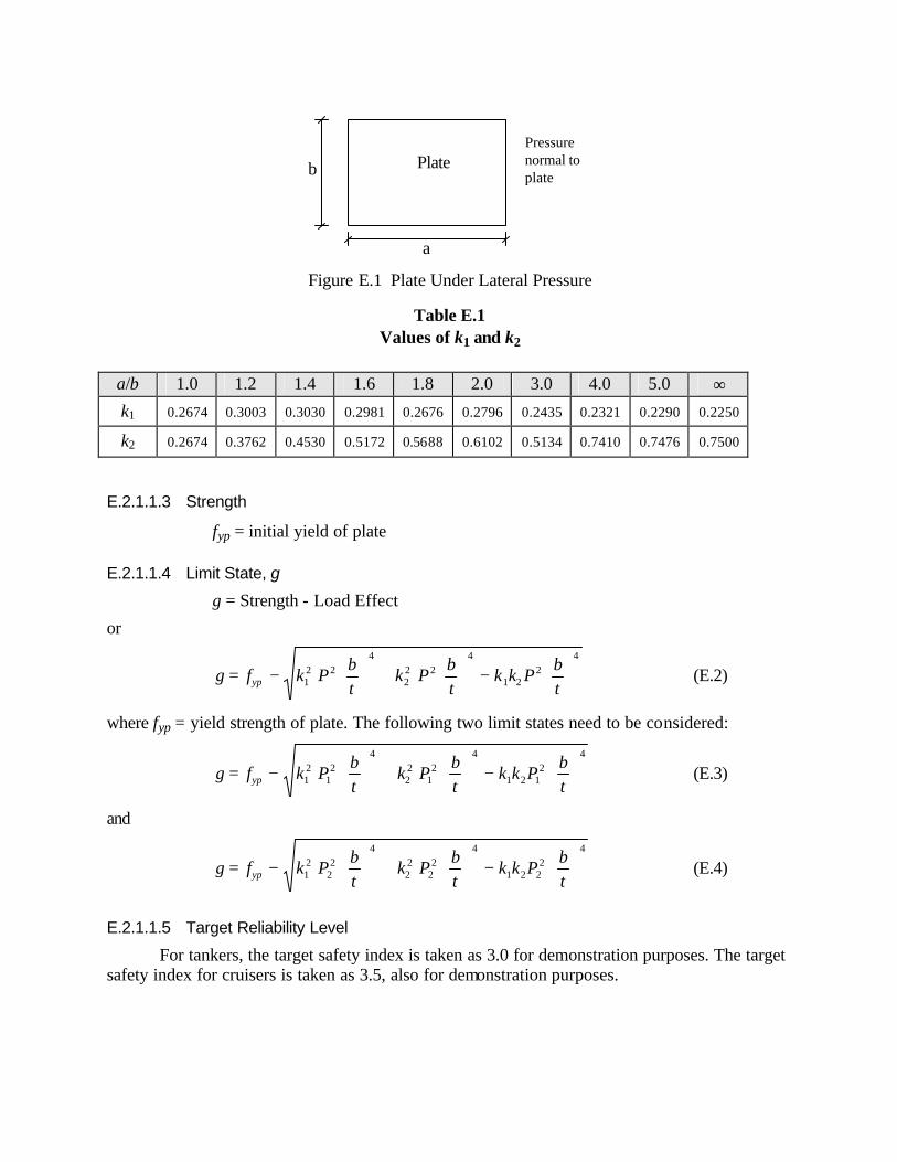
PlatePressurenormal toplate
a
b
Figure E.1 Plate Under Lateral Pressure
Table E.1 Values of k1 and k2
a/b 1.0 1.2 1.4 1.6 1.8 2.0 3.0 4.0 5.0 ∞ k1 0.2674 0.3003 0.3030 0.2981 0.2676 0.2796 0.2435 0.2321 0.2290 0.2250
k2 0.2674 0.3762 0.4530 0.5172 0.5688 0.6102 0.5134 0.7410 0.7476 0.7500
E.2.1.1.3 Strength
fyp = initial yield of plate
E.2.1.1.4 Limit State, g
g = Strength - Load Effect
or
g f k Pbt
k Pbt
k k Pbtyp= −
+
−
1
2 24
22 2
4
1 22
4
(E.2)
where fyp = yield strength of plate. The following two limit states need to be considered:
g f k Pbt
k Pbt
k k Pbtyp= −
+
−
1
212
4
22
12
4
1 2 12
4
(E.3)
and
g f k Pbt
k Pbt
k k Pbtyp= −
+
−
1
222
4
22
22
4
1 2 22
4
(E.4)
E.2.1.1.5 Target Reliability Level
For tankers, the target safety index is taken as 3.0 for demonstration purposes. The target safety index for cruisers is taken as 3.5, also for demonstration purposes.

E.2.1.2 Serviceability (Deformation) Limit State
E.2.1.2.1 Loads
The following service loads need to be considered:
1. Stillwater S 2. Waves W 3. Green-seas on deck GS
E.2.1.2.2 Load Effect
The following two types of pressure can be computed based on service conditions:
1. Service hydrostatic pressure (P1) due to S and W P1 = PS+PW
2. Service green-seas pressure (P2) due to GS P2
The deflection (w) due to these loads can be evaluated as follows (Hughes, 1988; Mansour, 1986):
w kPbEt
= 3
4
3 (E.5)
where k3 = a coefficient that depends on the aspect ratio of a plate (a/b, such that a ≥ b) and its boundary conditions, t = plate thickness, E = modulus of elasticity, and P = either P1 or P2. The deflection (w) can be computed for either the hydrostatic pressure or the green-seas pressure.
E.2.1.2.3 Strength
wa = limit on deflection
E.2.1.2.4 Limit State, g
g = Strength - Load Effect
or
g w kPbEta= − 3
4
3 (E.6)
This formulation can be used to size the plate, i.e., select t and b. The loads in this serviceability condition should be non-factored service loads.
E.2.1.2.5 Target Reliability Level
For tankers, the target safety index is taken as 3.0 for demonstration purposes. The target safety index for cruisers is taken as 3.5, also for demonstration purposes.

E.2.1.3 Strength Limit
Two methods to compute the ultimate strength of a plate are available: (1) Mansour Method (1986); and (2) Hughes Method (1988). One of these methods can be selected and used in future studies.
E.2.1.3.1 Loads
The following extreme loads need to be considered:
1. Stillwater S 2. Waves W 3. Green-seas on deck GS
E.2.1.3.2 Load Effect
The following two types of ultimate pressure can be computed based on extreme conditions:
1. Ultimate hydrostatic pressure (Pu1) due to S and W Pu1 = PuS+PuW
2. Ultimate green-seas pressure (Pu2) due to GS Pu2
E.2.1.3.3 Strength (in pressure units)
Two methods to compute the ultimate strength of a plate are available: (1) Mansour Method (1986); and (2) Hughes Method (1988). One of these methods will be selected and used in this study. One of the following two methods can be used to compute a plate’s ultimate strength (R) in pressure units:
1. Mansour’s Method (1986)
R kf t
abyp= 4
2
(E.7)
where k4 = a coefficient that depends on the aspect ratio of a plate (a/b, such that a ≥ b) and its boundary conditions, t = plate thickness, and fyp = the plate’s yield strength.
2. Hughes’ Method (1988)
For a specified maximum permanent set (wu), the strength (R) is
Rf
E B
ba
TB
ba
ba B
B
b a
BRyp
w=− +
+
+
+ + −
− ++
2
2 2
4
2 2
1 52
11 0 6
1 0 5 1 33 1
10 32
ν ν ν ν.
. ..
/.
(E.8)
where
Bbt
f
Eyp=

Rw
B twu=
− +24 115
2
2
ν ν.
[ ]T R RR
w w
w
= − −
≤>
1 11
11
3 1 3( )
/
in which ν = Poisson’s ratio = 0.3 (deterministic), E = modulus of elasticity, and plate size such that a > b. These strength equations can be reduced for a special case of wu by assigning a value for it.
E.2.1.3.4 Limit State, g
g = Strength - Load Effect
The following two states need to be considered:
g = R - Pu1 (E.9)
and
g = R - Pu2 (E.10)
E.2.1.3.5 Target Reliability Level
For tankers, the target safety index is taken as 3.0 for demonstration purposes. The target safety index for cruisers is taken as 3.5, also for demonstration purposes.
E.2.2 Unixial Compressive Stress
This section is limited to the ultimate limit state.
E.2.2.1 Loads
The following extreme loads need to be considered:
1. Stillwater S 2. Waves W 3. Dynamic effects D
E.2.2.2 Load Effect
The stress, f, is a function of S, W, and D, and can be computed as
f = fS + fW + fD (E.11)
E.2.2.3 Strength
The strength Fu of a plate subjected to uniaxial compression parallel to the dimension a, as shown in Fig. E.2, is given by one of the following two cases, as provided in AISC (1994) and described by Mansour (1986):

Platein-planecompression
a
b
Figure E.2 Plate Subjected to In-Plane Compression.
1. For a/b ≥1.0
Ff
B
B B
if B
if B
if B
u
yp
=
−
−
≥
≤ <
<
πν
2
2 2
2
3 1
225 125
10
35
10 35
10
( )
. .
.
.
. .
.
(E.12)
2. For a/b < 1.0
Ff
CB
u
ypu= + − +
≤α α0 08 1 1
11 0
2
2
. ( ) . (E.13)
where
C
B
B B
if B
if B
if B
u =
−
−
≥
≤ <
<
πν
2
2 2
2
3 1
2 25 125
10
35
10 35
10
( )
. .
.
.
. .
.
(E.14)
and α = a/b.
E.2.2.4 Limit State, g
g = Strength - Load Effect
g = Fu - f (E.15)
or
1. For a/b ≥1.0

g
f f f
f f f
f f f
if
if
if
yp s w
yp s w
yp s w
=
−− −
−
− −
− −
≥
≤ <
<
πν β
β β
β
β
β
2
2 2
2
3 1
2 25 1 25
3 5
1 0 3 5
10
( )
. .
.
. .
.
(E.16)
2. For a/b < 1.0
g f C f fyp u s w= + − +
− − ≤α αβ
0 08 1 11
102
2
. ( ) . (E.17)
where
C
if
if
if
u =
−
−
≥
≤ <
<
πν β
β β
β
β
β
2
2 2
2
3 1
2 25 125
10
35
10 35
10
( )
. .
.
.
. .
.
(E.18)
and
α = a/b
Bbt
f
Eyp= (E.19)
E.2.2.5 Target Reliability Level
For tankers, the target safety index is taken as 3.0 for demonstration purposes. The target safety index for cruisers is taken as 3.5, also for demonstration purposes.
E.2.3 Edge Shear
This section is limited to the ultimate limit state.
E.2.3.1 Loads
The following extreme loads need to be considered:
1. Stillwater S 2. Waves W 3. Dynamic effects D

E.2.3.2 Load Effect
The shear stress, τ, is a function of S, W, and D, and can be computed as follows, as provided in AISC (1994) and described by Mansour (1986):
τ = τS + τW + τD (E.20)
E.2.3.3 Strength
The strength formulation is taken similar to AISC LRFD (1994) formulation that accounts for both buckling and post-buckling strength. The ultimate strength (τu) is given by
τu = τcr + τpcr (E.21)
where τcr = critical or buckling strength, and τpcr = post-buckling strength using tension field action. The buckling strength can be computed based on one of the following three conditions that correspond to shear yield, inelastic buckling and elastic buckling:
τ
τ
τπ
ν
πν
τπ
ντ
τπ
ντ τ
πν
τπ
ν
cr
yp
pr s
s
pr s
yp
pr s
yp
s
pr
s
pr
kE t
b
kE t
b
forbt
kE
fork
Ebt
k E
forbt
k E
=−
−
≤−
−≤ ≤
−
≥−
2
2
2
2
2
2
2
2
2
2 2
2
2
2
12 1
12 1
12 1
12 112 1
12 1
( )
( )
( )
( )( )
( )
(E.22a)
(E.22b)
(E.22c)
where τyp = yield stress in shear, and τpr = proportional limit in shear which can be taken 0.8τyp. The yield stress in shear (τyp) is given by
τ ypypf
=3
(E.23)
where fyp = the yield stress of the plate. The value of the constant ks is
ka bs = +5
52( / )
(E.24)
The post buckling strength is

ττ
αpcr
yp crf=
−
+
3
2 1 2 (E.25)
where α = a/b.
E.2.3.4 Limit State, g
g = Strength - Load Effect
g = τu - τ (E.26)
E.2.3.5 Target Reliability Level
For tankers, the target safety index is taken as 3.0 for demonstration purposes. The target safety index for cruisers is taken as 3.5, also for demonstration purposes.
E.2.4 Biaxial Compressive Edge Stresses
This section is limited to ultimate limit state.
E.2.4.1 Loads
The following extreme loads need to be considered:
1. Stillwater S 2. Waves W 3. Dynamic effects D
E.2.4.2 Load Effect
The stresses, fX and fY, are functions of S, W, and D, and can be computed as
fX = fSX + fWX + fDX (E.27) fY = fSY + fWY + fDY
E.2.4.3 Strength
The strength needs to be obtained in both the X and Y directions of a plate. These values can be computed as described in Section E.2.1.3. They are denoted FuX and FuY, respectively. Then an interaction equation can be used to describe the strength, as provided in AISC (1994) and described by Mansour (1986).
E.2.4.4 Limit State, g
g = Strength - Load Effect
The limit state is given by the following interaction equation:

gfF
fF
fF
fF
X
uX
Y
uY
X
uX
X
uX
= −
+
−
1
2 2
η (E.28)
where
η =
≥
< <
=
0 25 30
10 30
10
. .
. .
.
linear interpolation
3.2exp(0.25 ) - 2B
forab
forab
forab
(E.29)
E.2.4.5 Target Reliability Level
For tankers, the target safety index is taken as 3.0 for demonstration purposes. The target safety index for cruisers is taken as 3.5, also for demonstration purposes.
E.2.5 Biaxial Compression and Edge Shear
This section is limited to ultimate limit state.
E.2.5.1 Loads
The following extreme loads need to be considered:
1. Stillwater S 2. Waves W 3. Dynamic effects D
E.2.5.2 Load Effect
The stresses, fX, fY, and τ, are functions of S, W, and D, and can be computed as
fX = fSX + fWX + fDX
fY = fSY + fWY + fDY (E.30)
τ = τS + τW + τD
E.2.5.3 Strength
The compressive strength needs to be obtained in both the X and Y directions of a plate. These values can be computed as described in Section E.2.1.3. They are denoted FuX and FuY, respectively. The shear strength (τu) needs to be obtained as described in Section E.2.3. Then an interaction equation can be used to describe the strength, as provided in AISC (1994) and described by Mansour (1986).

E.2.5.4 Limit State, g
g = Strength - Load Effect (E.31)
The limit state is given by the following interaction equation:
gf
Ff
FX
uX
Y
uY u
= −
+
+
1
2 2 2ττ
(E.32)
E.2.5.5 Target Reliability Level
For tankers, the target safety index is taken as 3.0 for demonstration purposes. The target safety index for cruisers is taken as 3.5, also for demonstration purposes.
E.2.6 Biaxial Compression, Edge Shear and Lateral Pressure
This section is limited to the ultimate limit state.
E.2.6.1 Loads
The following extreme loads need to be considered:
1. Stillwater S 2. Waves W 3. Dynamic effects D 4. Green-seas on deck GS
E.2.6.2 Load Effect
The load effects can be classified into two types, in-plane stresses and pressures. The stresses, fX, fY, and τ, are functions of S, W, and D, and can be computed as
fX = fSX + fWX + fDX
fY = fSY + fWY + fDY (E.33)
τ = τS + τW + τD
The pressures, Pu1 and Pu2 can be computed as
1. Hydrostatic pressure (Pu1) due to S and W Pu1
2. Green-seas pressure (Pu2) due to GS Pu2
E.2.6.3 Strength
A strength model for this case that is suitable for the development of a reliability-based design format is needed. Additional work in this area is needed.
E.2.6.4 Limit State, g
g = Strength - Load Effect (E.34)
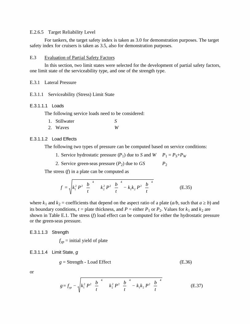
E.2.6.5 Target Reliability Level
For tankers, the target safety index is taken as 3.0 for demonstration purposes. The target safety index for cruisers is taken as 3.5, also for demonstration purposes.
E.3 Evaluation of Partial Safety Factors
In this section, two limit states were selected for the development of partial safety factors, one limit state of the serviceability type, and one of the strength type.
E.3.1 Lateral Pressure
E.3.1.1 Serviceability (Stress) Limit State
E.3.1.1.1 Loads
The following service loads need to be considered:
1. Stillwater S 2. Waves W
E.3.1.1.2 Load Effects
The following two types of pressure can be computed based on service conditions:
1. Service hydrostatic pressure (P1) due to S and W P1 = PS+PW
2. Service green-seas pressure (P2) due to GS P2
The stress (f) in a plate can be computed as
f k Pbt
k Pbt
k k Pbt
=
+
−
1
2 24
22 2
4
1 22
4
(E.35)
where k1 and k2 = coefficients that depend on the aspect ratio of a plate (a/b, such that a ≥ b) and its boundary conditions, t = plate thickness, and P = either P1 or P2. Values for k1 and k2 are shown in Table E.1. The stress (f) load effect can be computed for either the hydrostatic pressure or the green-seas pressure.
E.3.1.1.3 Strength
fyp = initial yield of plate
E.3.1.1.4 Limit State, g
g = Strength - Load Effect (E.36)
or
g f k Pbt
k Pbt
k k Pbtyp= −
+
−
1
2 24
22 2
4
1 22
4
(E.37)

where fyp = yield strength of plate. The limit state, as given by Eq. (E.37), can be expressed as follows:
gf
bt
k k k k
P PypS W=
+ −
− −2
12
22
1 2
(E.38)
Equation (E.38) provides a strength minus load effect expression of the limit state. The objective herein is to develop one strength reduction factor and one load amplification factor. Therefore, the strength (R) needs to be treated as a single random variable by expression Eq. (E.38) as
g = R - PS - PW (E.39a)
where
Rf
bt
k k k k
yp=
+ −2
12
22
1 2
(E.39b)
E.3.1.1.5 Derivation of Partial Safety Factors
Values of design factors used to derive the partial safety factors is summarized in Table E.2.
The probabilistic characteristics of the strength, R, need to be assessed based on the underlying basic random variables that define R according to Eq. (E.39b). Equation (E.39b) includes the variables b, t, a, k1, k2, and fyp. Although a does not appear in Eq. (E.39b), it is needed for computing k1 and k2. Monte Carlo simulation can be used to assess the probabilistic characteristics of the strength, R, by generating b, t, and fyp, and then feeding the generated values in Eq. (E.39b) with the appropriate k1 and k2 to obtain R values. This process needs to be repeated for the ranges of the key parameters (see Table E.2).
The results of the simulation were expressed in the form of nominal to mean value of R, the coefficients of variation of R, and distribution type of R. Statistical goodness of fit tests were used to determine the distribution of R.
Table E.2 Values of Design Factors Used in Derivation of Partial Safety Factors
Target Safety Index, β0 Tanker Cruiser
3.0 3.5
Yield Strength of Plate Nominal Bias (mean/nominal) COV Distribution
34 ksi 1.05 0.07
Normal Geometry Mean of b/a
2, 3, 4

Mean of b/t Std. Dev. of b or a Mean of t Std. Dev. of t Distribution of a, b, and t
50, 100, 150 0.125 in
0.25, 0.375, 0.5 in 0.0156 in Normal
Loads Stillwater Wave
Dist Normal EVD
COV 0.20 0.10
µW /µS 0.4 to 1.2 (Sec. E.3.1) 1.5 to 1.7 (Sec. E.3.2)
Poisson’s Ratio, ν 0.30 Modulus of Elasticity, E Mean COV Distribution
29,500 ksi
0.05 Normal
The number of simulation cycles was set at 200 which is adequate for all practical purposes as was demonstrated for the uniaxial compression of plates (Section E.3.2). The results of the simulation of R are summarized in Tables E.3a and E.3b. The distribution type was determined to be either normal or lognormal. A lognormal probability distribution for R was used in this study. The simulation results were based on mean to nominal ratio of fyp to be 1, not 1.05. Therefore, the recommended strength reduction factor needs to be revised by multiplying it by 1.05.
Table E.3a Mean to Nominal Strength Ratio ( R /Rn)
(for aspect ratios of 2, 3, and 4, respectively)
b/t Ratio Thickness 50 100 150
0.250
0.375
0.500
1.0055 1.0047 1.0033 1.0023 1.0020 1.0023 1.0019 1.0013 1.0011
1.0046 1.0045 1.0033 1.0027 1.0018 1.0014 1.0018 1.0015 1.0010
1.0040 1.0034 1.0028 1.0025 1.0019 1.0013 1.0009 1.0011 1.0010

Table E.3b Coefficient of Variation of Strength (R)
(for aspect ratios of 2, 3, and 4, respectively)
b/t Ratio Thickness (in) 50 100 150
0.250
0.375
0.500
.1440
.1442
.1343
.1069
.1109
.1120
.0976
.0972
.0921
.1404
.1494
.1413
.1144
.1067
.1064
.1004
.0969
.0930
.1434
.1383
.1372
.1115
.1093
.1077
.0934
.0932
.0949
The results of the simulation of R were used to develop partial safety factors for tankers based on the limit state of Eq. (E.39a). The partial safety factors were computed for several selected cases that cover the assumed ranges of the parameters b, t, a, k1, k2, and fyp. The resulting mean strength to stillwater load ratios based on a target reliability of 3.0, and the corresponding partial safety factors, are summarized using Tables E.4a and E.4b, respectively. The partial safety factors are also shown in Fig. E.1. Based on these results, the following preliminary average values are recommended for tankers:
Strength reduction factor (φ) = 1.05(0.78) = 0.82
Stillwater load factor (γS) = 1.37
Wave load factor (γW) = 1.08
Table E.4a Ratios of Mean for Strength/Stillwater Load (β = 3.0)
Ratios of Means for Strength/Stillwater Load
COV (Fu) 0.4 0.6 0.8 0.9 1.2
0.08 2.180627 2.42421 2.677333 2.807645 3.213074 0.14 2.484273 2.773078 3.069825 3.220969 3.684295
Table E.4b Partial Safety Factors
(for COV(R) of 0.08 and 0.14, respectively), β = 3.0
Ratios of Means for Wave/Stillwater Load

Partial Safety Factors 0.4 0.6 0.8 0.9 1.2 Strength Reduction
Factor (φ) 0.864813 0.717148
0.859929 0.710847
0.857622 0.706849
0.857478 0.705614
0.860179 0.704374
Stillwater Load Factor (γS)
1.472304 1.373342
1.444281 1.346652
1.410704 1.320271
1.392142 1.307362
1.334447 1.270576
Wave Load Factor (γW)
1.033828 1.020626
1.067278 1.040968
1.106793 1.062041
1.128169 1.072665
1.191143 1.103788
a. Strength Reduction Factor for Plates Under Lateral Pressure
0.4
0.6
0.8
1
0.3 0.4 0.5 0.6 0.7 0.8 0.9 1 1.1 1.2 1.3Mean Stillwater/Wave Ratio
COV=0.08COV=0.14
Figure E.1a Partial Safety Factors for Plates Under Lateral Pressure
(Target β = 3.0)
a. Stillwater Load Factor for Plates Under Lateral Pressure
1
1.2
1.4
1.6
0.3 0.4 0.5 0.6 0.7 0.8 0.9 1 1.1 1.2 1.3Mean Stillwater/Wave Ratio
COV=0.08COV=0.14
Figure E.1b Partial Safety Factors for Plates Under Lateral Pressure
(Target β = 3.0)

a. Wave Load Factor for Plates Under Lateral Pressure
1
1.2
1.4
1.6
0.3 0.4 0.5 0.6 0.7 0.8 0.9 1 1.1 1.2 1.3Mean Stillwater/Wave Ratio
COV=0.08COV=0.14
Figure E.1c Partial Safety Factors for Plates Under Lateral Pressure
(Target β = 3.0)
Similar calculations were performed for cruisers using a target reliability of 3.5, and the corresponding partial safety factors are summarized in Tables E.5a and E.5b, respectively. The partial safety factors are also shown in Fig. E.2. Based on these results, the following preliminary average values are recommended for cruisers:
Strength reduction factor (φ) = (1.05)0.75 = 0.79
Stillwater load factor (γS) = 1.42
Wave load factor (γW) = 1.11
Table E.5a Ratios of Mean for Strength/Stillwater Load (β = 3.5)
Ratios of Means for Strength/Stillwater Load
COV (Fu) 0.4 0.6 0.8 0.9 1.2
0.08 2.330699 2.584979 2.852561 2.991901 3.431348 0.14 2.717296 3.026376 3.345818 3.509285 4.013547

Table E.5b Partial Safety Factors
(for COV(R) of 0.08 and 0.14, respectively), β = 3.5
Ratios of Means for Wave/Stillwater Load Partial Safety Factors 0.4 0.6 0.8 0.9 1.2 Strength Reduction
Factor (φ) 0.841219 0.676507
0.836493 0.670302
0.835464 0.666763
0.836454 0.665927
0.84308 0.666544
Stillwater Load Factor (γS)
1.542791 1.427241
1.508419 1.396512
1.464543 1.36545
1.439425 1.349968
1.363046 1.305003
Wave Load Factor (γW)
1.044591 1.02757
1.08983 1.053454
1.148339 1.081773
1.181291 1.096623
1.274878 1.141835
a. Strength Reduction Factor for Plates Under Lateral Pressure
0.4
0.6
0.8
1
0.3 0.5 0.7 0.9 1.1 1.3Mean Stillwater/Wave Ratio
COV=0.08COV=0.14
Figure E.2a Partial Safety Factors for Plates Under Lateral Pressure
(Target β = 3.5)
a. Stillwater Load Factor for Plates Under Lateral Pressure
1
1.2
1.4
1.6
0.3 0.5 0.7 0.9 1.1 1.3Mean Stillwater/Wave Ratio
COV=0.08COV=0.14

Figure E.2b Partial Safety Factors for Plates Under Lateral Pressure (Target β = 3.5)
a. Wave Load Factor for Plates Under Lateral Pressure
1
1.2
1.4
1.6
0.3 0.5 0.7 0.9 1.1 1.3Mean Stillwater/Wave Ratio
COV=0.08COV=0.14
Figure E.2c Partial Safety Factors for Plates Under Lateral Pressure
(Target β = 3.5)
E.3.1.1.6 Use of Partial Safety Factors
The resulting partial safety factors can be used to design plates to meet the serviceability condition of first yield at the center of a simply-supported plate by satisfying the following safety checking equation:
φ γ γf
bt
k k k k
P PypS S W W
+ −
≥ +2
12
22
1 2
(E.40)
The stillwater and wave pressures, in this case, need to be specified for meeting a serviceability condition; for example, they can be taken as the annual extreme loads.
E.3.2 Uniaxial Compressive Stress
This section is limited to the ultimate limit state.
E.3.2.1 Loads
The following extreme loads need to be considered:
1. Stillwater S 2. Waves W 3. Dynamic D
E.3.2.2 Load Effect
The stress, f, is a function of S, and W, and can be computed as
f = fS + fW (E.41)

f = fS + fW + fD (E.42)
E.3.2.3 Strength
The strength Fu is given by one of the following two cases:
1. For a/b ≥ 1.0
Ff
B
B B
if B
if B
if B
u
yp
=
−
−
≥
≤ <
<
πν
2
2 2
2
3 1
2 25 1 25
1 0
3 5
1 0 3 5
1 0
( )
. .
.
.
. .
.
(E.43)
2. For a/b < 1.0
Ff
CB
u
ypu= + − +
≤α α0 08 1 1
11 0
2
2
. ( ) . (E.44)
where
C
B
B B
if B
if B
if B
u =
−
−
≥
≤ <
<
πν
2
2 2
2
3 1
2 25 125
1 0
35
1 0 35
10
( )
. .
.
.
. .
.
(E.45a)
α = a/b (E.45b)
and
Bbt
f
Eyp= (E.45c)
E.3.2.4 Limit State, g
g = Strength - Load Effect (E.46)
g = Fu - f (E.47)
The limit states for only stillwater and wave loads is given by the following cases:
1. For a/b ≥1.0

g
fB
f f
fB B
f f
f f f
if B
if B
if B
yp S W
yp S W
yp S W
=
−− −
−
− −
− −
≥
≤ <
<
πν
2
2 2
2
3 1
2 25 125
35
10 35
10
( )
. .
.
. .
.
(E.48)
2. For a/b < 1.0
g f CB
f fyp u S W= + − +
− −α α0 08 1 11
2
2
. ( ) (E.49)
with the limitation given by Eq. (E.44). Dynamic loads can be considered as described later in this section.
E.3.2.5 Derivation of Partial Safety Factors
The partial safety factors for this limit state were developed for demonstration purposes using the values of Table E.2. The limit state is given by:
g = Fu - fS - fW
The above equation provides a strength minus load effect expression of the limit state. The objective herein is to develop one strength reduction factor and one load amplification factor. Therefore, the strength (Fu) needs to be treated as a single random variable. The moments method for computing partial safety factors requires the probabilistic characteristics of both Fu, fS, and fW.
The probabilistic characteristics of the strength, Fu, need to be assessed based on the underlying basic random variables that define Fu. These variables are a, b, t, fyp, and E. Monte Carlo simulation can be utilized to assess the probabilistic characteristics of the strength, Fu, by generating a, b, t, fyp, and E, and then feeding the generated values in the strength equation to obtain Fu values. This process needs to be repeated for the ranges of the key parameters.
The results of the simulation were expressed in the form of nominal to mean value of R, the coefficient of variation of R, and distribution type of R. Statistical goodness of fit tests were used to determine the distribution type of R.
The results of the simulation were expressed in the form of nominal to mean value of Fu, the coefficient of variation (COV) of Fu, and the distribution type of Fu. The number of simulation cycles was set at 100, which is adequate for all practical purposes based on the charts provided in Fig. E.3 for a typical set of an estimated mean, coefficient of variation, and the coefficient of variation of the sample mean for Fu. The results of the simulation of Fu are summarized in Tables E.6a and E.6b. The distribution type for Fu was determined to be either normal or lognormal. A lognormal probability distribution for R was used in this study. The strength R has a mean to nominal ratio of about 1.03. This ratio is needed to revise the resulting

strength reduction factor by multiplying it by 1.03. The maximum and minimum strength ratios are 1.043, and 1.006, respectively. The maximum and minimum COV of strength are 0.08, and 0.04, respectively.
1.025
1.03
1.035
1.04
1.045
1.05
25 50 75 100 300 500 1000 2000 5000 7000 10000
Number Of Cycles
Mea
n Fu
/Fun
Figure E.3a Estimated Mean, Coefficient of Variation, and Coefficient of Variation
of Sample Mean for Fu
0
0.02
0.04
0.06
0.08
25 50 75 100 300 500 1000 2000 5000 7000 10000
Number of Cycles
CO
V(F
u)
Figure E.3b Estimated Mean, Coefficient of Variation, and Coefficient of Variation
of Sample Mean for Fu
0
0.002
0.004
0.006
0.008
0.01
25 50 75 100 300 500 1000 2000 5000 7000 10000
Number of Cycles
CO
V(S
ampl
e M
ean
of F
u/Fu
n)
Figure E.3c Estimated Mean, Coefficient of Variation, and Coefficient of Variation
of Sample Mean for Fu

Table E.6a Mean to Nominal Strength Ratio ( F / Fu un )
b/t a/b t (in) 50 100 150
0.250 1.0329 1.018011 1.024373 2 0.375 1.038469 1.02323 1.026731 0.500 1.041583 1.029762 1.027882 0.250 1.032268 1.024927 1.02176 3 0.375 1.040157 1.025057 1.009896 0.500 1.041212 1.021123 1.02741 0.250 1.043122 1.006146 1.030023 4 0.375 1.035976 1.029633 1.020356 0.500 1.031797 1.03514 1.021249 0.250 1.031613 1.036789 1.037933
0.4 0.375 1.028689 1.032298 1.027118 0.500 1.037029 1.031344 1.031872 0.250 1.029244 1.024514 1.028243
0.6 0.375 1.03174 1.032877 1.032408 0.500 1.040443 1.031721 1.034645 0.250 1.023216 1.012801 1.019138
0.8 0.375 1.040286 1.011904 1.014104 0.500 1.039777 1.034836 1.020961

Table E.6b Coefficient of Variation of Strength (Fu)
b/t a/b t (in) 50 100 150
0.250 0.058425 0.079082 0.069403 2 0.375 0.060794 0.051048 0.057236 0.500 0.052735 0.047537 0.055338 0.250 0.057636 0.07937 0.069333 3 0.375 0.054287 0.053333 0.058584 0.500 0.048914 0.05461 0.051153 0.250 0.066812 0.076344 0.070726 4 0.375 0.060021 0.047904 0.059547 0.500 0.055633 0.050637 0.054919 0.250 0.070527 0.074448 0.070684
0.4 0.375 0.05726 0.058802 0.053054 0.500 0.052342 0.053527 0.056163 0.250 0.057405 0.050443 0.048501
0.6 0.375 0.055282 0.055728 0.061751 0.500 0.054886 0.057613 0.04678 0.250 0.062148 0.070153 0.071715
0.8 0.375 0.059722 0.051749 0.058896 0.500 0.052693 0.046299 0.059177
The simulation results of Fu were used to developed the partial safety factors based on the limit state equations. The partial safety factors were computed for several selected cases that cover the assumed ranges of the parameters a, b, t, fyp, and E. The partial safety factors for a target reliability of 3.0 (for tankers) are summarized in Tables E.7a and E.7b, and Fig. E.4. Based on these results, the following preliminary values are recommended for tankers:
Strength reduction factor (φ) = 0.85(1.03) = 0.88
Stillwater load factor (γS) = 1.3
Wave load factor (γW) = 1.25
Table E.7a Ratios of Means for Strength/Stillwater Load (β = 3.0)
Ratios of Means for Wave/Stillwater Load
COV (Fu) 1.5 1.6 1.7
0.04 3.43035 3.56950 3.70977 0.08 3.63750 3.78170 3.92710

Table E.7b Partial Safety Factors
(for COV(Fu) of 0.04 and 0.08, respectively), β = 3.0
Ratios of Means for Wave/Stillwater Loads Partial Safety Factors 1.5 1.6 1.7 Strength Reduction
Factor (φ) 0.960338 0.863684
0.961079 0.86526
0.961747 0.86679
Stillwater Load Factor (γS)
1.301221 1.285660
1.283616 1.270806
1.267817 1.257081
Wave Load Factor (γW)
1.328696 1.237262
1.341832 1.250783
1.352955 1.262827
a. Strength Reduction Factor for In-Plane Compression
0.4
0.6
0.8
1
1.4 1.5 1.6 1.7 1.8
Mean Wave/Stillwater Ratio
COV(Fu) = 0.04COV(Fu) = 0.08
Figure E.4a Partial Safety Factors for Plates Under Uniaxial Compressive Stress
(Target β = 3.0)
b. Stillwater Load Factor for In-Plane Compression
1
1.2
1.4
1.6
1.4 1.5 1.6 1.7 1.8
Mean Wave/Stillwater Ratio
COV(Fu) = 0.04
COV(Fu) = 0.08
Figure E.4b Partial Safety Factors for Plates Under Uniaxial Compressive Stress
(Target β = 3.0)

c. Wave Load Factor for In-Plane Compression
1
1.2
1.4
1.6
1.4 1.5 1.6 1.7 1.8
Mean Wave/Stillwater Ratio
COV(Fu) = 0.04
COV(Fu) = 0.08
Figure E.4c Partial Safety Factors for Plates Under Uniaxial Compressive Stress
(Target β = 3.0)
The partial safety factors for a target reliability of 3.5 (for cruisers) are summarized in Tables E.8a and E.8b, and Fig. E.5. Based on these results, the following preliminary values are recommended for cruisers:
Strength reduction factor (φ) = 0.85(1.03) = 0.88
Stillwater load factor (γS) = 1.3
Wave load factor (γW) = 1.4
Table E.8a Ratios of Means for Strength/Stillwater Load (β = 3.5)
Ratios of Means for Wave/Stillwater Load
COV (Fu) 1.5 1.6 1.7
0.04 3.652 3.8048 3.9588 0.08 3.89665 4.0552 4.2151
Table E.8b Partial Safety Factors
(for COV(Fu) of 0.04 and 0.08, respectively), β = 3.5
Ratios of Means for Wave/Stillwater Load Partial Safety Factors 1.5 1.6 1.7
Strength Reduction Factor (φ)
0.95643 0.84844
0.9573 0.850685
0.95806 0.85277
Stillwater Load Factor (γS)
1.31339 1.3056
1.29422 1.28810
1.277271 1.27222
Wave Load Factor (γW)
1.45295 1.33345
1.46755 1.35085
1.479667 1.36593

a. Strength Reduction Factor for In-Plane Compression
0.4
0.6
0.8
1
1.4 1.5 1.6 1.7 1.8
Mean Stillwater/Wave Ratio
COV(Fu) = 0.04
COV(Fu) = 0.08
Figure E.5a Partial Safety Factors for Plates Under Uniaxial Compressive Stress
(Target β = 3.5)
b. Stillwater Load Factor for In-Plane Comprssion
1
1.2
1.4
1.6
1.4 1.5 1.6 1.7 1.8
Mean Stillwater/Wave Ratio
COV(Fu) = 0.04
COV(Fu) = 0.08
Figure E.5b Partial Safety Factors for Plates Under Uniaxial Compressive Stress
(Target β = 3.5)
c. Wave Load Factor for In-Plane Compression
1
1.2
1.4
1.6
1.4 1.5 1.6 1.7 1.8
Mean Stillwater/Wave Ratio
COV(Fu) = 0.04
COV(Fu) = 0.08
Figure E.5c Partial Safety Factors for Plates Under Uniaxial Compressive Stress
(Target β = 3.5)

E.3.2.6 Partial Safety Factors for the Load Combination of Stillwater, Wave, and Dynamic Loads
The partial safety factors for this load combination were developed for demonstration purposes using target reliability indexes of 3.0 and 3.5 for tankers and cruisers, respectively. The limit state is given by
g = Fu - fS - kW (fW + kD fD)
where kW and kD are the load combination factors that account for phase angles, as defined by Mansour (1994). Using the load factors that were developed for hull girder bending, the strength reduction factor can be reevaluated for plates under uniaxial compression. Appendix D shows the development of the load factors for hull girder bending. Therefore, the following preliminary values are recommended for tankers:
Load combination factors (kW) = 1.0
Load combination factors (kD) = 0.7
Strength reduction factor (φ) = 0.75(1.03) = 0.77
Stillwater load factor (γS) = 0.75
Wave load factor (γW) = 1.50
Dynamic load factor (γD) = 1.27
Similarly, preliminary values were developed for cruisers using the same load factors as tankers for demonstration purposes. The following values were obtained for cruisers:
Load combination factors (kW) = 1.0
Load combination factors (kD) = 0.7
Strength reduction factor (φ) = 0.72(1.03) = 0.74 Stillwater load factor (γS) = 0.75
Wave load factor (γW) = 1.50
Dynamic load factor (γD) = 1.27
E.3.2.7 Use of Partial Safety Factors
The resulting partial safety factors can be used to design plates to meet a strength limit state for plates under uniaxial compression by satisfying the following safety checking equations:
φ Fu ≥ γS fS + γW fW
φ Fu > γS fS + kW (γW fW + kD γD fD)
where Fu is computed according to Eqs. (E.43) through (E.45). The stillwater and wave stresses, in this case, need to be specified for meeting a strength condition; for example, they can be based on the life-time extreme loads, as defined in Appendix D.

APPENDIX F COMMENTARY: LIMIT STATE FUNCTIONS FOR STIFFENED PANELS
F.1 Discussion: Description of Stiffened Panel Failures
The stiffened panel forms the backbone of most of a ship’s structure. It is by far the most commonly used structural element in a ship; appearing in decks, bottoms, bulkheads, and side shell. The primary purpose of the panel is to absorb out of plane (or lateral) loads and distribute those loads to the ship’s primary structure. It also serves to carry part of the longitudinal bending stress because of the orientation of the stiffeners. The amount of in-plane compression or tension experienced depends primarily on the location of the panel. Deck panels tend to experience large in-plane compression and small lateral pressures. Bottom panels experience large in-plane tension and compression, but usually with very significant lateral pressures.
F.1.1 Stiffened Panel Definition
The definition of a stiffened panel (also called the gross panel), for this work, is a panel of plating which has stiffeners running in two orthogonal directions. This panel is bounded by other structure, which have significantly greater stiffness in the planes of the loads when compared to the panel and its stiffeners. These boundaries would be provided by structure, such as transverse bulkheads, longitudinal bulkheads, side shell, or large longitudinal girders (e.g., the CVK).
The collapse of a stiffened panel can be prevented by choosing the size of the transverse stiffeners so that they provide sufficient flexural rigidity to enforce nodes at the location of the transverse stiffeners. If the transverse stiffeners act as nodes, then the collapse of the stiffened panel is controlled by the strength of the longitudinally stiffened sub-panel.
F.1.2 Longitudinal Stiffened Sub-Panel Definition
A typical longitudinally stiffened sub-panel, as shown in Fig. F.1, is bounded on each end by a transverse struc ture which has significantly greater stiffness in the plane of the lateral load. The sides of the panel are defined by the presence of a large structural member which has greater stiffness in bending and much greater stiffness in axial loading. Such structural members as keels, bottom girders, longitudinal bulkheads, deck girders, etc., can act as the side boundaries of the panel. When the panel is located so as to be in a position to experience large in-plane compression, the boundary conditions for the ends are taken as simply-supported. The boundary conditions along the sides can also be considered simply-supported.

Gross Panel
Longitudinally StiffenedSub-Panel
Keel
Figure F.1 Longitudinally Stiffened Sub-Panel (Hughes, 1988)

Three types of loads affect the panel. Negative bending loads are the lateral loads due to uniform lateral pressure which causes the plate to be in tension and the stiffener flanges to be in compression. Positive bending loads are the lateral loads which put the plating in compression and the stiffener flange in tension. The third load type is uniform in-plane compression. This type of loading arises from the hull girder bending, and will be considered to be positive when the panel is in compression. These loads may act individually or in combination with one another.
F.2 Identification of Possible Modes of Failure
There are several failure modes involving the overall stiffened panel or gross panel. In design, often it is desirable to size members so that the failure mode is shifted from one type to another which is more easily quantified. In the case of stiffened panels, a collapse would be considered a catastrophic failure, while the collapse of a longitudinally stiffened sub-panel would not be nearly as disastrous.
Limit states which attempt to provide some control over the various failure modes of the stiffened panel are provided in this appendix. The three limit states discussed for the stiffened panel (or gross panel) should be used to check a design. Other means can be used to determine scantlings. The three limit states are:
1) Minimum transverse rigidity to prevent gross panel buckling
2) Biaxial compressive in-plane stress - serviceability limit
3) Uniform lateral pressure - ultimate limit state
Consequently, the first “limit state” considered for stiffened panels is one which will preclude stiffened panel collapse and turn the problem into one of sub-panel design. The other limit states investigated in this section are considered to be “checking equations” rather than ones used for determining scantlings.
When stiffened panel (or gross panel) collapse is prevented, the design problem shifts to prevent the buckling collapse of the longitudinally stiffened sub-panel. Three failure modes and corresponding limit states are provided in this appendix. They are all ultimate limit states for the longitudinally stiffened sub-panel. They are:
1) Compressive collapse of the stiffener flange - Mode I
2) Compressive collapse of the plate flange - Mode II
3) Combined compressive collapse of the plate flange and tensile failure of the stiffener flange - Mode III
F.3 Limit States for Stiffened Panel Failure
Three limit states will be considered for the stiffened panel (or gross panel). The first is intended as a checking limit which will ensure that overall stiffened panel collapse is prevented and the strength of the panel will depend on the longitudinally stiffened sub-panel. The second limit state considers the effects of transverse, as well as longitudinal, in-plane loads and is a serviceability limit state. The third limit state is an ultimate limit state which is intended to provide limits on panel deformation.

F.3.1 Minimum Transverse Rigidity to Prevent Gross Panel Buckling
This limit state is used to solve for the minimum required flexural rigidity of the transverse stiffeners. From this, a minimum required moment of inertia and section modulus can be found. As long as the moment of inertia and section modulus of the transverse stiffeners are larger than the prescribed value, the stiffened (or gross) panel failure will be controlled by the strength of the longitudinally stiffened sub-panel.
F.3.1.1 Definition of Terms
a = the length or span of the panel between transverse webs BP = breadth of the panel b = distance between longitudinal stiffeners C = panel stiffness parameter D = plate flexural rigidity = Et3/12(1-ν2) E = Young’s modulus
Ix,Iy = the moment of inertia of the plate-stiffener combination, longitudinal & transverse
N = number of longitudinal sub-panels in overall (or gross) panel γx, γy = flexural rigidity of the longitudinal and transverse stiffeners, respectively
F.3.1.2 Load Effect
This case does not have a real “load.” Rather, this is a measure that is based on the gross panel geometry, which will specify the minimum required ratio of the transverse flexural stiffness to the longitudinal flexural stiffness. It is given as
BCa n
P4
2 41
1π
+
(F.3.1)
F.3.1.3 Strength
The ratio of the flexural rigidity of the transverse stiffeners to the flexural rigidity of the longitudinal stiffeners,
γ
γy
x
y
x
y
x
EI
DbDaEI
I a
I b= × = (F.3.2)
F.3.1.4 Limit State, g
g = Strength - Load Effect
gI a
I b
B
Ca Ny
x
p= − +
4
2 41
1π
(F.3.3)

If the value of g is greater than zero, the transverse stiffeners will not deflect under the axial loading in the x-direction. If the deflection of the transverse stiffener is limited, the panel will not buckle as a gross panel, but will be forced to buckle as a longitudinally stiffened sub-panel.
F.3.2 Buckling Under Combined Loads - Orthotropic Plate Approach
When an explicit limit state function for the strength of the stiffened panel under in-plane loads is desired, the orthotropic plate approach can be considered. This approach accounts for both longitudinal and transverse in-plane loads. It treats the stiffened panel as a plate with different stiffness properties in each direction. The effect of the longitudinal and transverse stiffeners are “melted” into the plating.
F.3.2.1 Definition of Terms
a = the length or span of the panel between transverse webs BP = breadth of the panel b = distance between longitudinal stiffeners E = Young’s modulus k = buckling coefficient for a simply-supported plate under axial in-plane load
Ix,Iy = the moment of inertia of the combined plate and stiffener, longitudinal & transverse
Ipx,Ipy = the moment of inertia of the effective plating (alone) about the neutral axis of the combined plate and stiffener, in the longitudinal & transverse directions, respectively
NSX,NSY = ultimate longitudinal and transverse in-plane load from the stillwater hull girder bending moment, respectively
NWX,NWY = ultimate longitudinal and transverse in-plane load from the wave hull girder bending moment, respectively
F.3.2.2 Load Effect
1. Ultimate longitudinal in-plane load due to S and W:NX = NSX + NWX
2. Ultimate transverse in-plane load due to S and W: NY = NSY + NWY
F.3.2.3 Strength (Hughes, 1988)
( )N kB N
D
EI I
a bBX cr
p Y
y
x y
p
= − −
+
( )2 1 2
2
2
2
2πη
π (F.3.4)
where
(NX)cr = critical applied load in the x-direction η = torsional stiffness parameter

= I I
I Ipx py
x y
Dy = bending rigidity of the plate in the transverse direction
= E Iy / a
F.3.2.4 Limit State, g
g = Strength - Load Effect
g = (NX)cr - NX
F.3.3 Excessive Plastic Deformation of the Gross Panel
Excessive deformation of a stiffened panel (or gross panel) under hydrostatic pressure can be a limiting factor in some design situations. A procedure is presented here to allow expressing the requirement to avoid excessive plastic deformation as a limit state function.
F.3.3.1 Definition of Terms
a = the length of the longitudinal stiffener BP = breadth of the panel b = distance between longitudinal stiffeners δ = length of the transverse stiffener
Mt = plastic moment of transverse stiffener at center
Ml = plastic moment of longitudinal stiffener at center m = number of longitudinal stiffeners n = number of transverse stiffeners
F.3.3.2 Load Effect
1. Extreme hydrostatic pressure due to S and W: Pu1 = PuS + PuW
2. Extreme pressure due to green-seas on deck: Pu2
The hydrostatic pressure and the gree-seas pressure will have to be checked separately.
F.3.3.3 Strength
The strength is the stiffness of the gross panel under lateral pressure. An expression for ultimate strength can be given as (Mansour, 1977)
P na
c ( )+1 (F.3.5)
where Pc is a parameter representing stiffness, given as
Pm
m m BM
mB
Rcp
tp
c=+
++
+δ ( )( )
( )12
12
2 for m even (F.3.6)

PB
MmB
Rcp
cp
c= ++δ
2
1( ) for m odd (F.3.7)
with the value for Rc found as
Rn
n n aMc t=
++
δ ( )( )
12
for n even (F.3.8)
Rn a
Mc t=+δ
( )1 for n odd (F.3.9)
F.3.3.4 Limit State, g
g = Strength - Load Effect
gP n
aPc
u=+
−( )1
(F.3.10)
F.4 Longitudinally Stiffened Sub-Panel Failure
F.4.1 Background
When the in-plane and lateral loads act in combination, the plate-stiffener becomes a “beam-column.” Here, collapse is still the result of “failure of a flange” as it is in the case of a “column,” but the effect of bending moment M0 and deflection δ0 caused by the presence of a lateral load must be considered. For the purpose of this discussion, lateral deflections and in the direction of the stiffeners are considered as positive. Because we can have positive or negative bending moment due to the lateral load, either flange (the plate or the stiffener flange) can be the failure flange and the failure can be either tensile or compressive. This would seem to indicate that there are four possible collapse modes - either flange in tension or compression. In actuality, one of the modes, tensile failure of the plating, never occurs due to the neutral axis of the combined plate-stiffener being so close to the plating. The other three modes represent possible collapse mechanisms and are discussed briefly below. Much of the following discussion is after Chapter 14 of Hughes (1988), and the reader is directed there for further details.
F.4.1.1 Mode I - Compression Yield of the Stiffener Flange
Under the combination of axial compression and negative bending, the stiffener flange will be the compression flange. Collapse of the panel occurs as a result of compressive failure of the stiffener flange either by the entire section (plate and stiffener) reaching a full plastic moment, Mp, or by buckling of the stiffeners in compression. When there is a large amount of axial compressive stress fa, it directly increases the compressive stress in the stiffener flange that was due to the negative bending. This leads to early compressive yielding of the stiffener and a delay in the plate yielding. The result is that the combined plate-stiffener is unable to achieve a plastic hinge condition. Rather, the stiffener reaches its limit of stress absorption and becomes ineffective in carrying the load. The section is effectively reduced to the plating alone, which collapses shortly thereafter.

Figure F.2 is an interaction diagram showing the collapse mechanisms for a typical panel under lateral and in-plane loads. The vertical axis is the ratio of the bending moment from the lateral load, M0, to full plastic moment, Mp, at collapse. The horizontal axis is the ratio of the collapse value of the applied in-plane stress, fa,u, and the material yield stress, fY. Because the in-plane load is usually much greater than the lateral load, the analysis is usually to determine the level of in-plane stress needed for collapse given a specified level of lateral bending moment. The lateral bending moment M0 and deflection δ0 are those for a simply-supported beam experiencing a uniform lateral load. The curve from point A to point B in Fig. F.2 represents the Mode I failure mechanism.
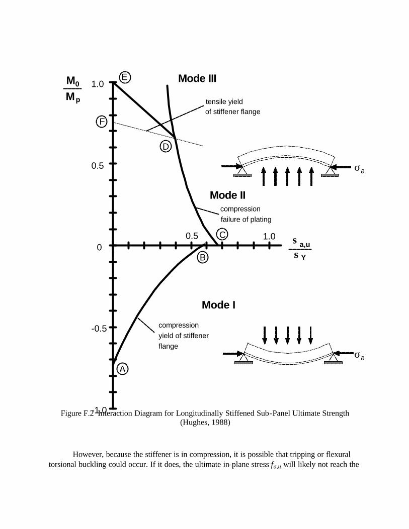
0
0.5
1.0
-0.5
-1.0
σa,u
σY
0.5 1.0
Mode I
Mode II
Mode IIIM0
pM
compression yield of stiffenerflange
tensile yieldof stiffener flange
compressionfailure of plating
σa
σa
A
B
C
D
E
F
Figure F.2 Interaction Diagram for Longitudinally Stiffened Sub-Panel Ultimate Strength (Hughes, 1988)
However, because the stiffener is in compression, it is possible that tripping or flexural torsional buckling could occur. If it does, the ultimate in-plane stress fa,u will likely not reach the

value indicated by curve AB. The common way to deal with this is to calculate fx,T, the elastic tripping stress for the beam-column and compare it to fY.
F.4.1.2 Mode II - Compression Failure of the Plating
The combination of in-plane compression and positive bending gives rise to the possibility of a Mode II failure mechanism. With small or moderate lateral loads (M0 / Mp ≈ 0.7 or less) collapse occurs due to compression failure of the plating. If the plate were to remain perfectly elastic through the range of loading the analysis would be that for a simple beam-column. However, for most welded plating the compressive collapse is a complex inelastic process. The curve from points C to D in Fig. F.2 represents the Mode II failure limit state.
Figure F.3 is a typical curve representing the relationship between average strain εa and total applied stress σpa for a welded plate. The curve shows that the relationship between εa and σpa becomes non-linear well before collapse. Plate failure is taken as the point on the curve where the plating has lost most of its stiffness. Usually this is the point where the tangent to the curve has reached some lower limiting value, and is represented on this figure as the value of the curve at a strain given by εult. Because it is easier to deal with stress in the analysis procedure, two levels of stress corresponding to a strain of εult are determined. The first is the actual value of the applied stress at failure, fpu. The second is the level of stress that would have been reached at a strain of εult if the plate had remained elastic. This value of stress is identified as fF. The curve in Fig. F.3 shows that the average value of stiffness of the plate is significantly less than the elastic material stiffness. We can account for this by defining a secant modulus Es = E⋅T, where T is given below (Hughes, 1988)
TB
= + − −
0 25 2
10 422..
ξ ξ (F.4.1)
where
ξ = 12 75
2+
.B
B = the plate slenderness ratio
= bt E
Yσ
t = plate thickness b = breadth of the panel

εa
fpa
fYp
fF
fpu
εult εYp
slope = Es = T E
slope = E
Figure F.3 Secant Modulus Concept

In order to account for this inelastic effect on the ultimate strength of the stiffened panel, a transformed section for the beam-column is defined. This is accomplished by defining a new effective width of plating to be used as one flange in the beam-column. The new transformed width is equal to the original width multiplied by the secant modulus transformation factor T. Given the transformed plating width, a whole new set of transformed section properties can be found. These transformed section properties are used in the determination of the panel ultimate stress.
F.4.1.3 Mode III - Combined Failure of the Stiffener and Plating
As the positive bending moment, M0, becomes very large, the Mode II description of collapse no longer is valid. When M0 is very large, there will be a large tensile stress in the flange of the stiffener. This tensile stress is somewhat reduced by the presence of the in-plane compressive stress, but if the bending moment is large enough, there will be tensile yielding in the stiffener flange as well as compressive failure of the plating. The point on the Mode II curve where this combined failure takes place is labeled point D in Fig. F.2.
When only bending loads are present, the collapse usually occurs at the value of the full plastic moment for the section. This is because the plastic neutral axis of the combined section often lies within the plating thickness. Point E on Fig. F.2 indicates the location of full plastic moment with no in-plane load. The straight line between points D and E represents the failure line for Mode III collapse. The actual collapse occurs slightly above this line, but the complicated interaction between stiffener tensile yielding and the compressive collapse of the plating makes this problem too difficult to calculate exactly with any efficiency.
To solve for the failure load, the equation for the line DE needs to be determined. This is accomplished by first determining the initial flange yield point D. The line shown in Fig. F.3 starting at point F and running through point D is used for this purpose. It is the line representing the first yielding of the stiffener flange in tension for a given applied moment M0. The intersection of this curve with the Mode II failure curve is found through an iterative solution to define point D. Once point D is known, an equation for line DE can easily be developed.
F.4.2 Mode I - Compression Failure of the Stiffener
F.4.2.1 Preliminary Remarks
This limit state is used to determine the strength of a longitudinally stiffened sub-panel experiencing in-plane compression and lateral pressure. The pressure is on the stiffener side, forcing the stiffener to deflect so that the stiffener flange is in compression and the plating is in tension. If the pressure causes a deflection of the stiffener away from the plating, or if there is a large enough initial deflection in this direction, a Mode I failure will not occur.
F.4.2.2 Definition of Terms
b = distance between longitudinal stiffeners bf = stiffener flange breadth
Cr = factor by which plate rotational restraint is reduced due to web bending
dw = stiffener web depth

E = Young’s modulus Fu = ultimate strength in Mode I
f1 = stress in the flange of the stiffener
fE = Euler’s buckling stress for the plate-stiffener combination
fX = factored extreme axial in-plane compressive stress from hull girder bending
fx,T = the elastic tripping stress for the beam-column
fys = average compressive yield stress of the stiffener
fp = proportional limit stress for the stiffener in compression G = shear modulus Ix, = the moment of inertia of the plate-stiffener combination, longitudinal
Isp = polar moment of inertia of stiffener about center of rotation
Isz = moment of inertia of the stiffener only about an axis through the centroid of the stiffener and parallel to the web
J = St. Venant’s torsional constant kw,kd = load combination factors
M0 = max bending moment in a simply-supported beam under a uniform lateral load
Ms = stillwater hull girder bending moment (nominal)
Mw = extreme wave induced hull girder bending moment (nominal)
Md = extreme dynamic (slamming or springing induced) hull girder bending moment (nominal)
m = number of longitudinal half-waves for stiffener tripping Ps = extreme lateral pressure due to stillwater condition
Pw = extreme lateral pressure due to wave action
P1 = factored lateral pressure applied to the stiffened panel (Mode I) t = plate thickness
tf = stiffener flange thickness
tw = stiffener web thickness
yf = distance from the centroidal axis of the cross-section to the mid-thickness of the stiffener flange
Z = hull girder section modulus to the location of interest ∆ = the initial eccentricity of the beam-column, typically taken as a/750 δ0 = the central deflection of a simply-supported beam under a uniform lateral load
Φ = magnification factor for in-plane compressive loading
γs = partial safety factor for stillwater bending moment
γw = partial safety factor for wave bending moment

γd = partial safety factor for dynamic bending moment
γPs = partial safety factor for stillwater pressure
γPw = partial safety factor for wave pressure
F.4.2.3 Load Effects
The loads can be classified into two types, in-plane stress and pressures. Both the axia l in-plane stress and the pressure are functions of have components which arise during the stillwater condition and the wave condition. Additionally, the in-plane stress has a component which is a function of the dynamic action, such as springing and slamming. For use in the limit states defined here, the input loads will be factored loads. The load fctors used are defined in Appendix A. The expression for the loads can be written as
1. Hydrostatic Pressure P1 = γPs Ps + kw (γPw Pw) (F.4.2)
2. Compressive Axial Stress fM k M k M
ZXs s w w w d d d=
+ +γ γ γ( ) (F.4.3)
The load effect for this limit state is the stress in the stiffener flange (f1) which results from the combination of applied pressure and axial compressive stress. An expression for f1 can be written as (Hughes, 1988):
f fM y
I
f A y
IXf
x
X f
x1
0 0= + ++( )δ
φ∆
(F.4.4)
where M0 and δ0 are the moment and deflection of a simply-supported beam under uniform lateral pressure P1. I, yf, and A are properties of the section composed of the combined stiffener and effective plating. ∆ is the initial stiffener deflection and φ is an amplification factor, given as:
Φ =−
1
1ff
fX
E
Ewhere is the Euler critical bucklingstress (F.4.5)
The first term in Eq. (F.4.4) is the compressive axial stress. The second term is the compressive stress in the stiffener flange for a simply-supported beam under a uniformly distributed lateral load. The third term is commonly known as the “P-Delta” effect. It accounts for the increase in compressive stress in the stiffener flange which results from the deflections caused by the lateral load and any initial deflection.
F.4.2.4 Strength
The strength side of the limit state is the critical stress for flexural torsional buckling, given by (Hughes, 1988)
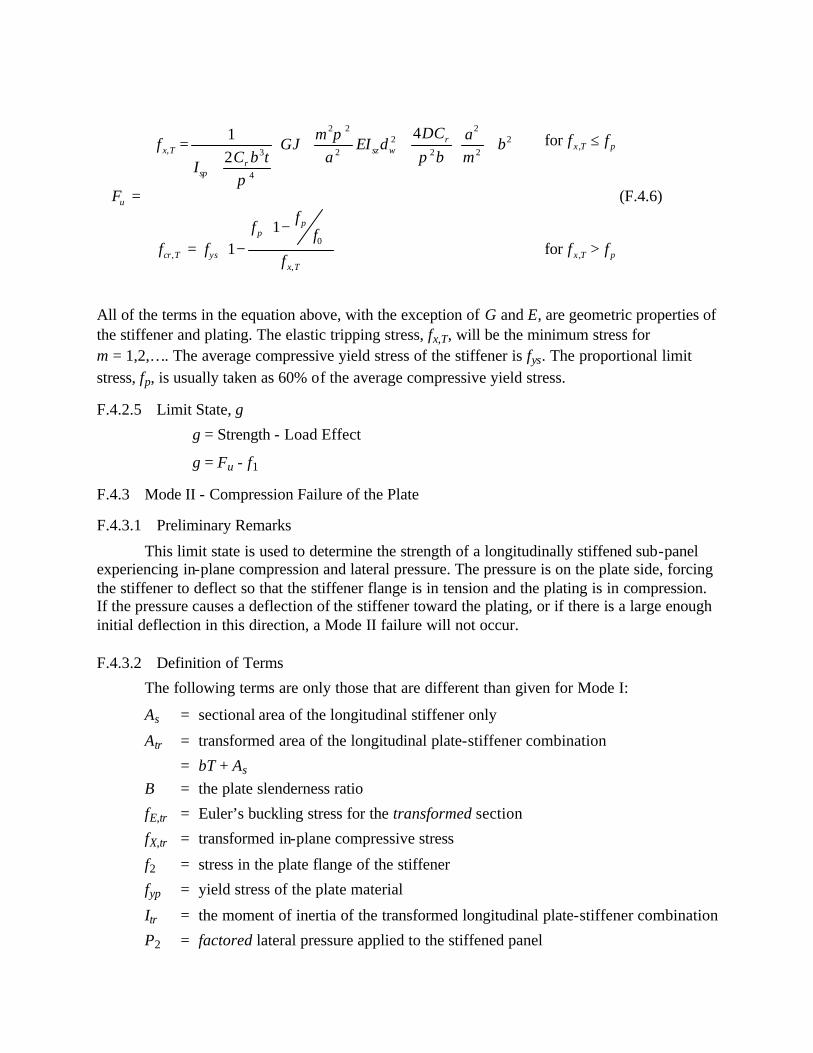
F
fI
C b tGJ
ma
EI dDC
bam
b
f ff
ff
f
f f
f f
u
x T
spr
sz wr
cr T ys
pp
x T
x T p
x T p
=
=+
+ + +
= −−
≤
>
,
,,
,
,
12
4
11
3
4
2 2
22
2
2
22
0
π
ππ
for
for
(F.4.6)
All of the terms in the equation above, with the exception of G and E, are geometric properties of the stiffener and plating. The elastic tripping stress, fx,T, will be the minimum stress for m = 1,2,…. The average compressive yield stress of the stiffener is fys. The proportional limit stress, fp, is usually taken as 60% of the average compressive yield stress.
F.4.2.5 Limit State, g
g = Strength - Load Effect
g = Fu - f1
F.4.3 Mode II - Compression Failure of the Plate
F.4.3.1 Preliminary Remarks
This limit state is used to determine the strength of a longitudinally stiffened sub-panel experiencing in-plane compression and lateral pressure. The pressure is on the plate side, forcing the stiffener to deflect so that the stiffener flange is in tension and the plating is in compression. If the pressure causes a deflection of the stiffener toward the plating, or if there is a large enough initial deflection in this direction, a Mode II failure will not occur.
F.4.3.2 Definition of Terms
The following terms are only those that are different than given for Mode I:
As = sectional area of the longitudinal stiffener only
Atr = transformed area of the longitudinal plate-stiffener combination
= bT + As B = the plate slenderness ratio
fE,tr = Euler’s buckling stress for the transformed section
fX,tr = transformed in-plane compressive stress
f2 = stress in the plate flange of the stiffener
fyp = yield stress of the plate material
Itr = the moment of inertia of the transformed longitudinal plate-stiffener combination
P2 = factored lateral pressure applied to the stiffened panel

T = transformation factor based on secant modulus concept yp,tr = distance from the centroidal axis of the transformed cross-section to the mid-
thickness of the plating ∆p = eccentricity of load due to use of transformed section
Φ = magnification factor for in-plane compressive loading
F.4.3.3 Loads Effect
The loads can be classified into two types, in-plane stress and pressures. Both the axial in-plane stress and the pressure are functions of have components which arise during the stillwater condition and the wave condition. Additionally, the in-plane stress has a component which is a function of the dynamic action such as springing and slamming. For use in the limit states defined here, the input loads will be factored loads. The load factors used are defined in Appendix A. The expression for the loads can be written as
1. Hydrostatic Pressure P2 = γPs Ps + kw (γPw Pw) (F.4.7)
2. Compressive Axial Stress same as Eq. (F.4.3)
The load effect for this limit state is the stress in the plate flange of the stiffener (f2) which results from the combination of applied pressure and axial compressive stress. An expression for f2 can be written as (Hughes, 1988):
f fM y
I
f A y
I
f A y
IX trp tr
tr
X tr tr p tr
tr
X tr tr p p tr
tr2
0 0= + ++
+,, , , , ,( )δ
φ∆ ∆
(F.4.8)
where M0, δ0 and ∆ are as defined before. The amplification factor φ is the same as in Eq. (F.4.5) except that fX,tr replaces fX. Itr, yp,tr, and A tr are properties of the transformed section composed of the combined stiffener and transformed plating. The transformed plating has a width btr, where btr = T × b. The transformation factor, T, is based on the secant modulus concept to account for the actual end shortening curve of welded steel plating. The transformation factor is given in Eq. (F.4.1).
The in-plane axial compressive stress must be modified to account for the reduced area over which the load is applied. The level of load has not decreased, therefore the level of stress must increase. The manner in which this is accounted for is to replace the axial stress fX by a transformed stress, such that fX,tr = fX(A/Atr).
The last term on the right-hand side of Eq. (F.4.8) is used to account for an induced load eccentricity due to decreased plate stiffness. Because the decreased stiffness of the plating was accounted for by using smaller plate width, the position of the neutral axis of the section has changed. The distance the neutral axis moved is ∆p. This last term is simply calculating the axial stress in the plating due to the shift in neutral axis.
F.4.3.4 Strength
The strength side of the limit state is determined by the value of applied axial stress in the beam-column which is sufficient to cause plate collapse. Because of the nonlinearity of the

modulus of elasticity in welded steel plating in compression, the failure stress is less than the yield stress in compression. The relationship is given as
FT
Tfu yp=
− 01. (F.4.9)
The factor T is as defined above and fyp is the yield strength of the plating in compression.
F.4.3.5 Limit State, g
g = Strength - Load Effect
g = Fu - f2
F.4.4 Mode III - Combined Failure of the Stiffener in Tension and the Plate in Compression
F.4.4.1 Preliminary Remarks
The Mode III collapse mechanism requires a combination of very high lateral pressure along with some in-plane compression. Because of the high lateral pressures required, it is not very likely to occur. However, the design should be checked to ensure that the possibility of Mode III failure does not exist. Therefore, rather than have a limit state which requires a certain specified level of safety, one which indicates if Mode III will be a problem will be used.
F.4.4.2 Definition of Terms
The following terms were not previously defined:
(M0)D = the value of moment at point D on Fig. F.2. This is the moment at the intersection of Eqs. (F.4.12) and F.4.13)
Mp = the moment required to develop a plastic hinge in the center of the beam-column under uniform lateral load only
yp,tr = distance from the centroidal axis of the transformed cross-section to the mid-thickness of the stiffener flange
F.4.4.3 Load Effect
The loads can be classified into two types, in-plane stress and pressures. Both the axial in-plane stress and the pressure are functionf of have components which arise during the stillwater condition and the wave condition. Additionally, the in-plane stress has a component which is a function of the dynamic action such as springing and slamming. For use in the limit states defined here, the input loads will be factored loads. The load factors used are defined in Appendix A. The expression for the loads can be written as
1. Hydrostatic Pressure P3 = γPs Ps + kw (γPw Pw) (F.4.10)
2. Compressive Axial Stress same as Eq. (F.4.3)

The load effect for this limit state is an expression which relates applied lateral pressure to a bending moment on the beam-column. Assuming that the beam-column is simply-supported, the expression is:
MP bau
0
2
8= (F.4.11)
where b is the spacing between stiffeners and a is the length of the stiffener.
F.4.4.4 Strength
The strength side of the limit state requires finding the combination of pressure and in-plane stress which causes simultaneous compression failure of the plating and tensile failure of the stiffener flange. The load combination at the intersection can be determined from the following equations:
TT
f fM y
I
f A y
I
f A y
Iyp X trp tr
tr
X tr tr p tr
tr
X tr tr p p tr
tr
−= + +
++
01 0 0. ( ),
, , , , ,δφ
∆ ∆ (F.4.12)
− = + ++
+f fM y
I
f A y
I
f A y
Iys X trf tr
tr
X tr tr f tr
tr
X tr tr p f tr
tr,
, , , , ,( )0 0δφ
∆ ∆ (F.4.13)
Equation (F.4.12) is the Mode II failure equation, with all of the variables as defined previously. The right-hand side of Eq. (F.4.13) is the stress in the stiffener flange. Due to the sign convention used in the analysis, compressive stress is positive. Consequently, tensile failure occurs when the stress reaches a value equal to the negative of the stiffener tensile yield stress (fys). The solution requires finding a combination of values for P3 and fx such that both Eqs. (F.4.12) and (F.4.13) are satisfied. These values will be designated (M0)D and (fx)D. This intersection corresponds to point D on the interaction diagram of Fig. F.2.
F.4.4.5 Limit State, g
This limit state is simply a safety check to preclude the possibility of combined failure. If the value of M0 is less than (M0)D or the full plastic moment Mp, then this failure mode will not occur. This limit can be expressed as:
MMM
D
p0
0<
Minimumof( )
(F.4.14)
F.5 Determining Partial Safety Factors for Longitudinally Stiffened Sub-Panel Failure
For demonstration purposes, one limit state for the longitudinally stiffened sub-panel was chosen for further development. In order to use any of the limit states expressed in this appendix in a design code, partial safety factors need to be developed. The limit states were developed so that they could be expressed in a Load and Resistance Factor Design (LRFD) format. This allows for the determination of load amplification partial safety factors and strength reduction partial safety factors. More detailed explanations on what partial safety factors are and how they fit in a

design equation are provided in Appendix A and Appendix C of this report. The discussion here will focus on how the partial safety factors were developed for the limit state chosen.
F.5.1 Compressive Failure of the Plate Flange - Mode II Collapse
The Mode II failure mode for the longitudinally stiffened sub-panel was chosen for demonstrating the develoment of partial safety factors. This limit state was chosen because it is represented by a fairly difficult, very non-linear expression. This type of failure is also the more likely mode of failure on modern ships. It occurs primarily in the decks of ships operating in a heavy sea. When the vessel begins to ship green-seas and experience large hull girder bending moments, this mode of failure is possible.
The partial safety factors for this limit state were developed for demonstration purposes using a reliability index, β0, of 3.5 for a tanker and 4.0 for a cruiser. The background on selecting these values for β0 is provided in Appendix B. The moments method for computing partial safety factors requires the probabilistic characteristics of both the strength and the load terms, Fu and f2, repsectively. The following describe how the probabilistic characteristics were developed.
F.5.1.1 Probabilistic Characteristics of the Strength
The strength side of the equation represents the compressive yield stress of a welded plate. This value is primarily a function of the plate compressive yield stress, fyp, and the plate width to thickness ratio, b/t, through the parameter B in Eq. (F.4.1). Chatterjee and Dowling (1976) found that the plate ultimate could be well approximated using the secant modulus factor T of Eq. (F.4.1) if corrected for the presence of residual stresses. Assuming that the ratio of the residual stresses to the yield stress is 0.10 has proven to be a very good approximation.
All four of the main parameters in the strength formulation given in Eq. (F.4.9) were considered to be random variables. The material yield stress was considered to be log-normally distributed with a COV of 0.08. The Young’s modulus was considered to be a normally distributed random variable with a COV of 0.05. The mean to nominal ratios for yield stress and Young’s modulus were taken as 1.0. This assumed that the designer would be using the actual mean of the variables. In the case of yield stress, if the actual mean was not available, the designer would be directed to multiply the nominal value by 1.15 to get a value to input into the design equation.
The plate width b, and plate thickness t, were treated somewhat differently. In ship construction, the variation in the dimensions of a part is not a function of the size of the part, but rather the ability to measure and control the measurements. As such, we determined that an appropriate means of including the random nature of plate thickness and plate width would be through the use of error terms. The plate thickness is the mean thickness plus a normally distributed error term with a mean of 0 and a standard deviation of 1/64th- inches. The error term for plate width is a normally distributed random variable with a mean of 0 and a standard deviation of 1/16th- inches. These values were chosen to reflect the manufacturer’s ability to use quality control to keep dimensions within tolerance.
To determine the probabilistic characteristics of the strength term Fu, these four random variables were used in a Monte Carlo simulation of Eq. (F.4.9). The simulations were run for 1000 cycles using a Latin Hypercube sampling technique. The mean to nominal ratio was

determined for each run, as was the COV of Fu. Each run was analyzed to determine the best fit probability distribution type by performing both a Chi-Square and a Kolmogorov-Smirnov test. To determine the effect of changing the mean dimensions on the probabilistic characteristics, different combinations of the variable mean values were tried. Table F.1 provides a summary of the parameters used to determine the geometry and characteristics of the plate for Eq. (F.4.9) as well as the range of parameters which were used in the Monte Carlo simulations.
Table F.1 Parameters Used In Monte Carlo Simulations
(Plate Geometry and Material Properties)
Parameter Description Values Used
t Plate Thickness (inches)
3/8, 1/2, 5/8
b/t Width to Thickness Ratio 40, 60, 80
fyp Average Compressive Yield Stress (psi)
34000, 42000, 60000
E Young’s Modulus (psi)
30 × 106
The results of the simulation over the range of the values shown in Table F.1 give the probabilistic characteristics of the strength. Fu was determined to be a normally distributed random variable with a mean-to-nominal ratio of 1.0 (rounded up from 0.9997) and a COV of 0.076.
F.5.1.2 Probabilistic Characteristics of the Load
The load side of the limit state contains the in-plane bending stresses and lateral pressures as well as all of the geometry variables needed to turn those loads into stress. The value presented for f2, given by Eq. (F.4.8) is the compressive stress in the plating due to the applied loads.
The usual procedure for developing a probabilistic-based design equation is to express the limit state as a simple function of the strength and loads. This allows the determination of partial safety factors which will let the designer produce a design with the specified level of safety. However, the limit state function in this case is extremely difficult and nonlinear. In order to develop a probabilistic design code, a number of simplifying assumptions needed to be made.
The first of these assumptions involved combining the weighted load effects in a simple manner prior to using them in Eq. (F.4.8). This is consistent with the approach taken by the American Institute of Steel Construction (AISC) in their 1994 LRFD Code. In LRFD-H1 for “beam-columns,” AISC uses factored loads in the limit state.
The load factors which make the most sense to use are the load factors for the ultimate strength of the hull girder. The hull girder bending moment can be directly converted to in-plane

stress through the knowledge of the section modulus. For the purpose of this demonstration, the loads were calculated as:
Hydrostatic Pressure P2 = γPs Ps + kw (γPw Pw) (F.5.1)
Compressive Axial Stress fX = γs fSX + kw (γw fWX + γd k d fDX) (F.5.2)
where the stress terms in Eq. (F.5.2) are found by dividing the appropriate hull girder bending moments by the section modulus of the hull. The statistical characteristics for the random variables used in the Monte Carlo simulation are provided in Table F.2. Note that the analysis assumes that the actual mean values are known for all variables but the yield stress. The mean-to-nominal ratio (Bias in Table F.2) for yield stress is assumed to to be 1.15.
Table F.2 Statistical Information for Monte Carlo Simulation
Statistical Information Bias or Error Information Variable Mean COV Dist. Type Category Mean COV Dist. Type
t µt Error 0 1/64″ Normal
b µb Error 0 1/16″ Normal
a µa Error 0 1/16″ Normal
fyp µf 0.08 Log-normal Bias 1.15
E µE 0.05 Normal Bias 1.00
fSX µSX 0.20 Normal Bias 1.00
fWX µWX 0.10 EV Type I Bias 1.00
fDX µDX 0.30 EV Type I Bias 1.00
PS µPS 0.20 Normal Bias 1.00
PW µPW 0.10 EV Type I Bias 1.00
To limit the number of random variables in the simulation of the load term, an analysis on the importance of each variable was considered. Nikolaidis, et al. (1994) performed a sensitivity analysis for the formulation for sub-panel strength used in this report. They found that the resulting ultimate stress was not very sensitive to minor variations in stiffener geometry, but was sensitive to variations in plate width and thickness. Consequently, we chose to only simulate values for t, b, and a. All of the dimensions of the panel were based on the mean value of the thickness and a set of non-dimensional parameters. The parameters used and the range of values for which simulations were conducted are provided in Table F.3.

Table F.3 Parameters Used in Monte Carlo Simulations for the Load
(Geometry, Loads and Load Ratios)
Parameter Description Values Used
t Plate Thickness (inches) 3/8, 1/2, 5/8 b/t Width to Thickness Ratio 40, 60, 80 a/b Plate Aspect Ratio 2, 3, 4
fyp Average Compressive Yield Stress (psi) 34000, 42000, 60000
E Young’s Modulus (psi) 30 × 106
Ap/As Plate Area-Stiffener Ratio 3, 4, 5
Af /As Flange Area-Stiffener Area Ratio .55
λc Column Slenderness Parameter 0.15, 0.30, 0.45, 0.60
µSX Mean Stillwater Bending Stress (psi) 6000, 8000, 10000
µWX /µSX Wave Induced Stress-Stillwater Stress Ratio
1.6, 1.8, 3.0
µPS /µSX Mean Stillwater Pressure-Mean Stillwater Bending Stress Ratio
.0003, .00045, .0006
µPW/µSX Mean Wave Induced Pressure-Mean Stillwater Bending Stress Ratio
.00012, .00018, .00024
Over two hundred simulations of Eq. (F.4.8) were run using various combinations of the values for the parameters of Table F.3. Each simulation run consisted of 2000 cycles. Statistical analysis on the output values of f2 was performed and the distribution type of the data was determined. Both Chi-Square and Kolmogorov-Smirnov goodness of fit tests were performed on the data. The ratio of the mean value of f2 from each simulation run was compared to the value of f2 found by using the nominal values of the variable directly in Eq. (F.4.8). As a result of the simulations performed, the statistical characteristics of the load term were determined to be:
mean-to-nominal ratio 1.0
COV of f2 0.092
Distribution Type Lognormal

0
0.1
0.2
0.3
0.4
0.5
0.6
0.7
0.8
0.9
1
0 0.1 0.2 0.3 0.4 0.5 0.6 0.7 0.8 0.9 1 1.1
Experimental Strength Ratio
Pre
dic
ted
Str
eng
th R
atio
Faulkner Parametric SeriesFaulkner Weld Series
Horne Fixed-end
Horne Pin-endLehigh Fixed-end
Lehigh Pin-endMurray
SmithUSNA
Mode I failure by theory
Lateral pressure
Figure F.4 Predicted Strength versus Experimental Strength (Vroman, 1995)

F.5.1.3 Probabilistic Characteristics of Modeling Bias
In order to develop a reliability-based design code, knowledge of the statistical characteristics of the key variables is required. An additional source of uncertainty also needs to be characterized. This source is the uncertainty associated with the analytical model (or algorithm) used as the limit state equation. Unless the algorithm represents an exact solution, there will be some bias associated with using the algorithm. Vroman (1995) investigated what he called the “modeling uncertainty” associated with the use of the “standard algorithm” for longitudinally stiffened sub-panels. The “standard algorithm” is the same limit state as provided in Eq. (F.4.8) and used in this report.
Figure F.4, from Vroman (1995), compares the ultimate stresses measured in eighty-six experiments to the values of ultimate stress determined by Eq. (F.4.8). The stresses are expressed as ratios of the ultimate stress to the yield stress of the material. The test database is made up of a variety of types of tests conducted at seven different locations in the U.S., the U.K., and Australia. Most of the tests were of the single bay variety; that is, there were no transverse stiffeners. In these tests, the type of boundary conditions used had a large effect on the ability of the limit state equation to predict the failure stress. A limited number of tests, those conducted by Smith (1975) and those conducted at the U.S. Naval Academy (Vroman, 1995), were multi-bay tests. These tests generally provided results that were more consistent with the predicted values from the limit state equation.
A statistical analysis of the data presented in Fig. F.4 (Vroman, 1995), indicates that the modeling uncertainty associated with all of the tests can be represented as a random variable (the Bias) with the following characteristics:
mean value of Bias 0.91 COV of Bias 0.156 Distribution Type Normal
F.5.1.4 Calculation of the Partial Safety Factors Using FORM
With the information on the strength, load, and bias random variables, the partial safety factors for the Mode II Collapse limit state could be determined. A comuter program which utilized a First-Order Reliability Method (FORM) approach was used. The limit state equation could be written as
φS Fu = γB BM × γf f2 (F.5.3) where
φS = strength reduction factor
γB = bias amplification factor
γf = load amplification factor
BM = the modeling bias
The bias amplification factor is in Eq. (F.53) because of the manner in which the FORM approach determines partial safety factors. Each random variable in the limit state equation will have a partial safety factor associated with it. In order to make the design equation appear like other equations in the proposed design code, the bias amplification factor and the load

amplification factor are multiplied and their product is considered to be the partial safety factor for the loading. That is
γL = γB × γf (F.5.4)
It should be pointed out again that, at the beginning of the definition of this limit state, we chose to use factored loads in Eq. (F.4.8). The factored loads are developed in Eqs. (F.5.2) and (F.5.2) using partial safety factors from hull girder bending. In order not to confuse the designer with too many partial safety factors, we have chosen to move the load amplification factor, γL, to the strength side of the equation. This will involve the introduction of a modified partial safety factor for strength
φ φγ= S
L (F.5.5)
The FORM program was run for a variety of values for the loads and the partial safety factor φ was determined. Using a reliability index β0 of 4.0 for cruisers, φ was found to be 0.54. When using a β0 value of 3.5 for tankers, φ was determined to be 0.59. A complete description of the code statement for the Mode II collapse with a table providing the partial safety factors is given in Section 2.5.8 of this report.

APPENDIX G COMMENTARY: FATIGUE
G.1 Limit State Equations
G.1.1 The Characteristic S-N Approach
The fatigue strength of a component is characterized by a relationship between the constant amplitude stress and cycles to failure. For welded joints, the following is assumed. For a general reference, see Wirsching (1984) and Wirsching and Chen (1988).
1. Fatigue strength is given by the characteristic S-N curve,
N Sm = A (G.1)
2. The equation is value to S = 0, i.e., there is no endurance limit,
3. Miner’s rule is valid
Uncertainty in fagitue strength is evidenced by the large scatter in fatigue S-N data. This uncertainty is accounted for by treating the fatigue strength coefficient, A, as a random variable.
Fatigue damage is given as
DnA
E S m= ( ) (G.2)
From Miner’s rule, the equivalent constant amplitude stress is
S E Sem m' /[ ( )]= 1 (G.3)
where S is a random variable denoting range of a stress cycle selected at random. E(⋅) denotes “expected value.” Fatigue loading models are described in Section G.2. The prime indicates “best estimate.” Introduce stress modeling error as a random variable, B. Stress modeling error relates to the uncertainties associated with translating statistics on the long-term environment (waves) and operating history to stresses on components. This would include errors associated with the loading models and the computer codes for translating loads into member stresses (see Section G.2).
The actual Miner’s stress is
S B Se e= ' (G.4)
Thus, damage becomes
DnA
B Smem= (G.5)
Let damage D at failure be denoted as ∆. Uncertainties in the performance of Miner’s rule is accounted for by treating ∆ as a random variable. At failure (limit state)
D = ∆ when n = N (G.6)
where N is the total number of cycles to failure.
NA
B Smem
=∆
(G.7)

Fatigue failure occurs when the cycles to failure, N, is less than the intended service life, NS, of the component. But N is a random variable by virtue of its relationship with random variables A, ∆, and B. Development of reliability-based fatigue design criteria is discussed in Section E.4.
G.1.2 The Fracture Mechanics Approach
Not considered in this report, but should be included in the complete code.
G.2 Fatigue Stress and Stress Modeling Error
G.2.1 Fagitue Stress: The Hot Spot Stress vs. the Characteristic S-N Approach
There are two fundamental approaches which have been employed in fatigue design of welded joints. In the first approach, a suite of S-N curves are developed for characteristic weld detail. British standards have nine classifications. In practice, each welded detail to be analyzed must be identified with a specific curve in the menu. Fatigue stress is the nominal stress in the joint. The limitation of this approach is that many joints in a ship do not match geometry well with that of one of the standard S-N curves.
In a second approach, the fatigue stress is defined as the hot spot stress at the toe of the weld, where the stress concentration is the highest and where the fatigue crack is expected to initiate. Only one universal S-N curve is required to define fatigue strength for all welds. The limitation of this approach is that determination of the hot spot stress may require finite element analysis.
The former approach (characteristic S-N) will be the method used in this document. However, the method for determining safety factors described herein apply directly to the hot spot approach, as well.
G.2.2 Miner’s Stress, Se
Models employed by the marine industry to compute Miner’s stress are summarized in Table G.1.
Table G.1 Commonly Used Expressions for Miner’s Stress, Se [Wirsching (1984)]
1.Wave exceedance diagram (deterministic method)
S Sem
i im
i
= ∑ ζ
Si = stress range ζi = fraction of total stress ranges that Si is acting
2. Spectral method (probabilistic method)

S ff
mfe
mm
i i im
i0
0
22
1= +
∑(2 )
γ σ
f0 = average frequency of stresses Γ(⋅) = gamma function γi = fraction of time in ith seastate fi = frequency of wave loading in the ith seastate σi = RMS of stress process in ith seastate
3. Weibull model for stress ranges
S S ln Nm
em m
Sm= +
−
0 1[ ] /ξ
ξΓ
S0 = stress that is exceeded on the average once out of NS stress cycles ξ = Weibull shape parameter NS = total number of stress ranges in design life Γ(⋅) = gamma function
Varying levels of sophistication are available for analysis. The Weibull model is widely employed because it has a closed analytical form and, therefore, is easy to use. Additional information on the Weibull model is given in the next section. The most refined model would start with a scatter diagram of seastates, information on ship’s routes and operating characteristics, and employ a ship response computer program to provide a detailed history of stress ranges over the service life of the ship. For this approach, one could use the wave exceedance diagram or the spectral method as given in Table G.1.
G.2.3 The Weibull Model
The Weibull distribution has the following form for the cumulative distribution function,
F xx
( ) exp= − −
1δ
ξ
(G.7a)
where ξ and δ are the Weibull shape and scale parameters, respectively. It is convenient to express δ in terms of the design stress, S0 [Fatigue Handbook (1985), Wirsching and Chen (1988)]
δ = S0 [ln NS]-1/ξ (G.7b)
S0 is the stress range that is exceeded, on the average, only once every NS cycles. NS is the service life.
The Weibull distribution has been shown to provide a good fit to the long-term distribution of stress ranges in ships [Munse, et al. (1983)]. And because of its ease of use, it is often employed as a default model for life prediction analysis.

The model parameters from the form given in Table G.1 are NS, the service life in cycles, S0, the stress that is exceeded on the average once during NS, and ξ, the Weibull shape parameter. S0 is often interpreted as the design stress range to compute the peak stress for quasi-static failure modes, e.g., buckling and fracture.
Measured values of ξ and S0 are given in Table G.2 for some commercial ships. Default values of ξ for preliminary design considerations are given in Table G.3. The recommended values in Table G.3 are assumed values based on measured values such as those of Table G.2.
G.2.4 Stress Modeling Error
Stress modeling error refers to the systematic and random errors in estimating the maximum stress that a component will see during its design life and/or the magnitude of the fatigue stresses. The process of computing stresses in a component includes the following steps: (1) defining and modeling the environment, (2) translating the environ-ment into forces on the structure, (3) computing the response of the structure to the environmental loads, (4) computing nominal stresses in the components, and (5) com-puting the stresses to be used for design, e.g., the stress at points of stress concentration. Assumptions are made at each step, and all of the assumptions contain some uncertainty.
In this exercise to develop design criteria, physical uncertainty associated with the environment and the choice of operations are included with modeling error to form a total stress uncertainty. This uncertainty is quantified with a random variable, B. The mean (or median) of B relates to bias or systematic errors, and the coefficient of variation refers to random errors. The lognormal distribution is assumed for B because: (1) it is known that the lognormal is a good default distribution, and (2) the easy to use lognormal format can be employed herein to derive safety factors.
Table G.2 Some Measured Values of ξ and S0
[after Munse, et al. (1983)]
Ship
Approximate Displacement
(dwt)
Weibull Shape Parameter, ξ
Midship Bending
Stress (once in 108 cycles)
S0 (ksi)
Notes
Bulk Carriers Wolverine State Mormacscan California Bear Fontini
15,300 12,500
13,400 74,000
1.2 1.3 1.0 1.0 0.9
16.5 12.0 10.0 18.0 29.5
No. Atlantic So. America
Tankers Idemitsu Maru
206,000 66,500
1.0 0.8
12.3 30.0

Follis Esso Malasia Universe Ireland
191,000 327,000
0.8 0.7
21.8 18.7
Container Ships (SL-7) SeaLand McLean
50,300
1.2
34.1
Dynamics Included
Table G.3 Default Values of ξ
Weibull Shape Parameter, ξ
• Commercial Ships
Exposure to normal operational seastates
1.0
Exposure to extreme environments
1.2
• Naval Ships
Non-combatants 1.2
Combatants 1.4
Four levels of refinement of stress analysis are proposed. Approximate tolerance levels for each are given in Table G.4. Note that the intervals are not symmetric because the lognormal is not symmetric. Also given are some guidelines regarding the choice of level. Safety factors for cases other than these can be obtained by interpolation.
Table G.4 Levels of Uncertainty in Stress Prediction
Level
Coefficient of Variation CB
Tolerance Level*
1 0.30 0.55 to 1.80
2 0.25 0.61 to 1.65
3 0.20 0.67 to 1.50
4 0.15 0.74 to 1.35

*Assume: (1) ~B = 1.0; (2) B has a lognormal distribution; and (3) tolerances based on ± 2 standard deviations.
Some general guidelines regarding the choice of level.
Level 1 Use for a safety check expression using the design stress. Default values are assumed for the Weibull shape parameter and the service life. There is little confidence in the estimates of the loads.
Level 2 The Weibull model for long-term stress ranges is used. Reasonable estimates of the parameters are available.
Level 3 The Weibull model for long-term stress ranges is used with good estimates of the parameters obtained from tests on similar ships. The histogram and/or spectral methods with only moderate confidence of the parameters.
Level 4 A comprehensive dynamic and structural analysis of the ship over its predicted service history has been performed as the basis for the input for the histogram or spectral method.

G.3 Fagitue Strength Statistics
G.3.1 S-N Curves Used in British and Norwegian Rules
Fatigue design curves for various welded details were developed by the British [BS 5400 (1980)] and used also in a Norwegian standard [NS 3472 (1984)]. See also Gurney (1979). Welded joints are classified into several categories, an abbreviated form of which is given in Table G.5. Extensive test data were obtained on each detail.
Table G.5 Abbreviated Joint Classification for BS 5400 and DnV
Fatigue Requirements
Presented here is only a summary description. For complete details, see Gurney (1979).
Class Description
B
Plain steel in the as-rolled condition, or with cleaned surfaces, but with no flame cut edges or re-entrant corners. Full penetration butt welds, parallel to the direction of applied stress, with the weld overfill dressed flush with the surface and finish-machined in the direction of stress, and with the weld proved free from significant defects by non-destructive examination
C
Butt or fillet welds, parallel to the direction of applied stress, with the welds made by an automatic submerged or open arc process and with no stop-start positions within the length. Transverse butt welds with the weld overfill dressed flush with the surface and with the weld proved free from significant defects by non-destructive examination.
D
Transverse butt welds with the welds made in the shop either manually or by an automatic process other than submerged arc, provided all runs are made in the flat position.
E Transverse butt welds that are not class C or D.
F Load-carrying fillet welds with the joint made with full penetration welds with any undercutting at the corners of the member dressed out by local grinding.
F2
Load-carrying fillet welds with the joint made with partial penetration or fillet welds with any undercutting at the corners of the member dressed out by local grinding.
G Parent metal at the ends of load-carrying fillet welds which are essentially parallel to the direction of applied stress.
W
Weld metal in load-carrying joints made with fillet or partial penetration welds, with the welds either transverse or parallel to the direction of applied stress (based on nominal shear stress on the minimum weld throat area).
The basic model describing fatigue strength is
N Sm = A (G.8)

Least squares estimates of m and A, and the standard deviation of log life given log stress (and therefore the coefficient of variation of A and life, N), are computed from the data of each detail. The results are shown in Table G.6. Note that it is implicitly assumed that log life given stress has a normal distribution, and therefore life given stress (and therefore A) has a lognormal distribution.
Also shown in Table G.6 are the values of A (denoted as A0) that define the design curve. The design curve is defined by the mean minus two standard deviations on a log basis (see Section G.3.3). A plot of the design curves is given in Figure G.1.
Table G.6 Statistical Summaries of Fatigue Data and Design S-N Curves
used in British and Norwegian Rules
Ref: BS 5400 (1980), NS 3472 (1984)
STATISTICAL SUMMARY DESIGN CURVE
Median A
~
COV of N
A0
Class(a) m MPa ksi (%) MPa ksi(b)
B 4.0 2.34 E15 1.04 E12 44 1.01 E15 4.47 E11
C 3.5 1.08 E14 1.25 E11 50 4.23 E13 4.91 E10
D 3.0 3.99 E12 1.21 E10 51 1.52 E12 4.64 E 9
E 3.0 3.29 E12 1.00 E10 63 1.04 E12 3.17 E 9
F 3.0 1.73 E12 5.28 E 9 54 6.30 E11 1.92 E 9
F2 3.0 1.23 E12 3.75 E 9 56 4.30 E11 1.31 E 9
G 3.0 5.66 E11 1.73 E 9 43 2.50 E11 7.63 E 8
W 3.0 3.68 E11 1.12 E 9 44 1.60 E11 2.88 E 8
Notes: (a) See Table F.5 for detail (b)Median minus two standard deviations on a log basis
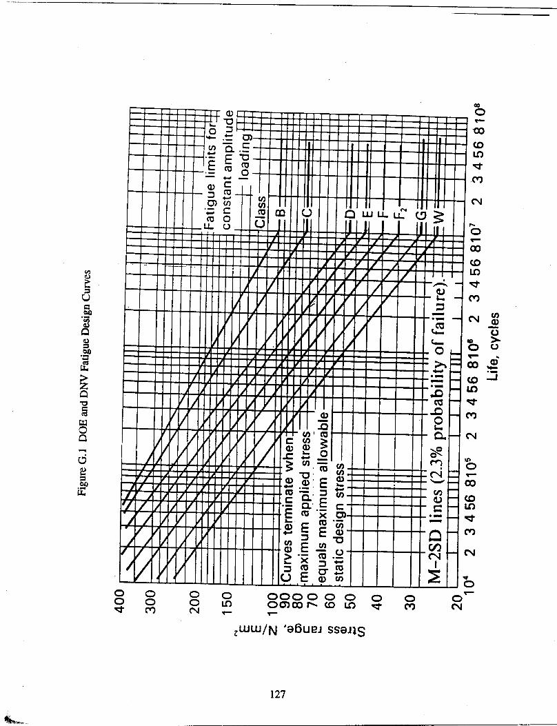

G.3.2 S-N Data on Welded Joints [after Munse, et al. (1983)]
More extensive summaries of welded joint data were provided by Munse, et al. (1983) on an SSC project. Munse correlated available data in the literature with typical welded detail in a ship. He identified 53 different joint details (shown in Figure G.2) and provided S-N data for each.
Parameters for each detail obtained by least squares analysis of the data are summarized in Table G.7.
Table G.7 Statistical Summary of S-N Fatigue Data
[Munse, et al. (1983)]
DETAIL (See Fig. E.2)
m log10 A
~ CN
1 (all steels) 1M 1H 1Q 1(F) 2 3 3(G) 4 5 6 7B 7P 8 9 10M 10H 10Q 10(G) 10A 10A(G)† 11 12 12(G) 13 14 14A†
5.729 12.229 15.449 5.199 4.805 6.048 5.946 6.370 5.663 3.278 5.663 3.771 4.172 6.549 9.643 7.589 12.795 5.124 7.130 5.468
-- 5.765 4.398 5.663 4.229 7.439
--
15.55 25.36 32.04 14.91 13.78 15.82 14.80 15.52 14.22 9.65 14.22 11.23 11.46 16.44 19.59 16.63 25.92 13.65 16.93 14.14
-- 13.77 11.69 14.12 12.12 16.96
--
0.75 0.71 0.91 0.68 0.60 0.64 0.63 0.74 0.61 0.48 0.61 0.53 0.51 0.81 0.90 0.88 0.96 0.76 0.94 0.79 --
0.68 0.43 0.60 0.45 0.91 --

Table G.7 -- continued
DETAIL (See Fig. E.2)
m log10 A
~ CN
35 36 36A 38 38(S) 40** 42 46** 51(V) 52(V)
3.808 6.966 5.163 3.462
10.225 3.533 7.358 4.348 3.818 4.042
10.75 15.15 12.88 10.17 17.39 9.71 16.98 10.67 10.93 11.24
0.28 0.63 0.46 0.36 0.88 --
0.83 --
0.07 0.19
Mean Value Std. Dev.
-- --
-- --
0.62 0.23
* Only three test points available. Not enough data to calculate δ f ** These are the estimated values † Data scatter makes evaluation questionable †† Range in lives is small--extrapolation questionable
NOTES:
B = bending stress (F) = flame cut surfaces P = principal stress (G) = surfaces have been ground M = mild steel flush H = high strength low alloy steel (V) = average shear based on net Q = quenched and tempered steel area of web (S) = shear stress on fasteners or welds

Table G.7 -- continued
DETAIL (See Fig. E.2)
m log10 A
~ CN
15 16 16(G) 17 17(S) 17A 17A(S) 18 18(S) 19 19(S) 20 20(S) 21 (1/4″ weld)* 21 (3/8″ weld)* 21(S) 22 23 24 25 25A 25B 26 27 27(S) 28 28(F)†† 30 30A 31** 31A 32A 32B** 33 33(S)
4.200 4.631 6.960 3.736 7.782 3.465 7.782 4.027 9.233 7.472 7.520 4.619 6.759
14.245 15.494 7.358 3.147 3.187 3.187 7.090 8.518 6.966 3.348 3.146 5.277 7.746
-- 3.159 3.368 4.348 3.453 4.200 3.533 3.660
10.368
10.83 12.02 15.55 10.39 16.28 10.14 16.28 10.26 18.02 15.19 15.83 11.57 14.73 26.72 25.49 16.98 10.04 9.94 9.94 15.79 19.47 15.15 10.13 9.40 12.06 17.41
-- 9.87 10.58 10.67 10.13 10.83 9.71 9.86 19.59
0.43 0.58 0.95 0.34 0.65 0.39 0.65 0.65 0.75 0.93 0.93 0.66 0.93 -- --
0.83 0.32 0.13 0.13 0.78 0.91 0.63 0.61 0.58 0.54 0.81 --
0.31 0.10 --
0.44 0.43 --
0.50 0.81


G.3.3 Strength Modeling Error: Uncertainty in Miner’s Rule
Miner’s rule is a simple algorithm to predict fatigue life under random loads using constant amplitude data. Because it is a simple algorithm, it is expected that there will be significant errors in life predictions—and indeed, experimental results.
For an S-N curve, NSm = A, fatigue damage D is,
Dn E S
A
m
=( )
(G.9)
If Miner’s rule were perfect, then D = 1 at failure (n = N). But observed values of D in experimental studies have shown significant scatter. A comprehensive review of random fatigue tests on welded joints, provided by Gurney (1986), indicate significant uncertainty in the performance of Miner’s rule.
Upon extensive review of random fatigue test data [e.g., Wirsching and Chen (1988)], it was suggested modeling damage, D, at failure as a random variable, ∆, having a lognormal distribution with median equal to one and a coefficient of variation of 0.30. This model has been used by Wirsching and others in performing fatigue reliability analysis, but it is important to note that it is based on subjective judgment of available evidence, and is, in essence, a blanket or default recommendation.
In summary, damage at failure, ∆, is treated herein as a random variable, ∆
∆ ∆∆ ∆
~
( )~
.( ) .
lognormal
MedianCOV
= == =
100 30C
(G.10)
G.3.4 Definition of the Design Curve
The design S-N curve is defined as a “lower bound” of the data. In fact, it is a curve that is parallel to the mean curve shifted two standard deviations on a log basis to the left. The design curve, defined by A0, is shown in Fig. G.3.
The relationship between the design curve, A0, and the median, A, is given by (using natural logs) (NOTE: For lognormal distribution mathematics, one can employ either base e or base 10 logs. This paper follows the custom in fatigue reliability of using base 10 logs for fatigue data analysis (e.g., Table G.7) and base e for reliability analysis as follows. Confusion is avoided by noting that the median and coefficient of variation of the random variable are the same in both systems.)
ln A ln A ln A0 2= −~
σ (G.11)
The scatter factor is defined as
λ =~AA0
(G.12)


NA
B Smem
=∆
(G.15)
Assume that ∆, A, and B are lognormally-distributed random variables. Then N will have an exact lognormal distribution. There will be a closed-form solution for the probability of a fatigue failure prior to the end of the intended service life, NS.
pf = P (N ≤ NS) (G.16) But the analytical form follows the lognormal format. Thus,
pf = Φ (-β) (G.17)
where β is the safety index, defined for this limit state as
βσ
=ln N N S
ln N
( ~ / ) (G.18)
where
~~ ~
~NA
B Smem
=∆
(G.19)
and
{ }σ ln N A Bmln C C C= + + +( ) ( ) ( )1 1 12 2 2 2
∆ (G.20)
The tildes over the variables denote median values, and the C’s denote coefficients of variation.
For a safety check expression, it is necessary to specify: (1) statistics on the design variables; and (2) minimum allowable safety index, β0.
The basic design requirement is that the safety index describing the reliability of a component exceeds the minimum allowable, or target, safety index.
β ≥ β0 (G.21)
The value of β0 and the statistics on the design variables are used to derive the expression for the target damage level.
Nominal (deterministic) damage is computed as,
DN S
AS e
m
00
= (G.22)
and the safety check expression is
D0 ≤ ∆0 (G.23)
Letting β = β0 and D0 = ∆0, and combining Eqs. (G.12), (G.18), (G.19), (G.22), and (G.23), and solving for ∆0,
∆∆
00
=~
~ exp( )λβ σB m
ln N
(G.24)
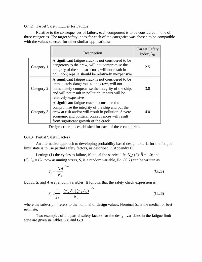
G.4.2 Target Safety Indices for Fatigue
Relative to the consequences of failure, each component is to be considered in one of three categories. The target safety index for each of the categories was chosen to be compatible with the values selected for other similar applications:
Description
Target Safety Index, β0
Category 1
A significant fatigue crack is not considered to be dangerous to the crew, will not compromise the integrity of the ship structure, will not result in pollution; repairs should be relatively inexpensive
2.5
Category 2
A significant fatigue crack is not considered to be immediately dangerous to the crew, will not immediately compromise the integrity of the ship, and will not result in pollution; repairs will be relatively expensive
3.0
Category 3
A significant fatigue crack is considered to compromise the integrity of the ship and put the crew at risk and/or will result in pollution. Severe economic and political consequences will result from significant growth of the crack
4.0
Design criteria is established for each of these categories.
G.4.3 Partial Safety Factors
An alternative approach to developing probability-based design criteria for the fatigue limit state is to use partial safety factors, as described in Appendix C.
Letting: (1) the cycles to failure, N, equal the service life, NS; (2) ~B = 1.0; and (3) CB = CS, now assuming stress, S, is a random variable, Eq. (G.7) can be written as
SA
NeS
m
=
∆1/
(G.25)
But Se, ∆, and A are random variables. It follows that the safety check expression is
SA
NeS
n A n
S
m
≤
11
γγ γ( ) ( )
/
∆ ∆ (G.26)
where the subscript n refers to the nominal or design values. Nominal Se is the median or best estimate.
Two examples of the partial safety factors for the design variables in the fatigue limit state are given in Tables G.8 and G.9.

Table G.8 Partial Safety Factors: Level 1 Stress Analysis (CS = 0.30)
γS γ∆ γA
Category 1 (β0 = 2.5) B C D E F G
1.91 1.84 1.79 1.75 1.77 1.79
0.88 0.86 0.84 0.85 0.84 0.84
1.76 1.68 1.59 1.55 1.59 1.26
Category 2 (β0 = 3.0) B C D E F G
2.20 2.09 2.03 1.95 2.01 2.02
0.85 0.83 0.81 0.81 0.81
0.806
1.63 1.52 1.43 1.33 1.40 1.12

Table G.9 Partial Safety Factors: Level 3 Stress Analysis (CS = 0.20)
γS γ∆ γA
Category 1 (β0 = 2.5) B C D E F G
1.49 1.44 1.40 1.37 1.39 1.39
0.82 0.81 0.79 0.80 0.79 0.79
1.52 1.42 1.32 1.26 1.33 1.07
Category 2 (β0 = 3.0) B C D E F G
1.62 1.55 1.50 1.46 1.49 1.50
0.78 0.77 0.79 0.77 0.75 0.75
1.38 1.26 1.17 1.06 1.15
0.925
Category 3 (β0 = 4.0) B C D E F G
1.85 1.82 1.65 1.70 1.73 1.75
0.72 0.69 0.59 0.65 0.64
0.634
0.978 0.957 0.901 0.852 0.943 0.752
G.4.4 Simplified Criteria Based on Peak Stress
The peak stress is defined as the expected maximum stress over the service life. It can be defined as the stress that is exceeded, on the average, once during the service life. Simplified criteria based on the peak stress only, and using default values for the basis parameters, is derived in the following. A Level 1 stress analysis having a COV of B equal to 0.30 is assumed.
By deterministic analysis, damage is computed as (Eq. (G.22))
DN S
AS e
m
00
= (G.27)
And the safety check expression is, (Eq. (G.23))
D0 ≤ ∆0 (G.28)

where ∆0 is chosen on the basis of a Level 1 analysis and the appropriate value of β0 and S-N curve.
Assume a Weibull shape parameter of ξ = 1.0 and a service life NS = 108 cycles. Using the Weibull model for stress ranges (Table G.1), it follows that,
S S ln mem m m= +−
0810 1( ) ( )Γ (G.29)
Define the peak stress as Smax. Assuming that a peak has twice the magnitude of a trough (this is an assumption based on the fact that wave heights are typically larger than wave troughs, as measured from the mean. The relationship of Eq. (G.30) is commonly used in the offshore industry), the relationship between the design peak stress and stress range is,
S Smax =23 0 (G.30)
Upon combining Eqs. (G.27) through (G.30), it follows that the safety check expression, based on the design stress, is,
SA
max m
m
≤+
0 667 18 4210 1
1 0 08
1
. ( . )( )
/
/
ξ
ξ
∆Γ
(G.31)
Example: Determine the design stress for the C curve. The data is given in Table G.10. Also given in the table are results of calculations, and corresponding equation numbers, in the sequence of steps to derive a safety check expression
Smax ≤ 20.5 ksi

Table G.10 Data for Example
C curve m 3.5
~A (ksi units) 1.25 E11
A0 (ksi units) 4.91 E10
CA 0.50
Weibull Shape Parameter ξ 1.0
Median COV
∆ 1.0 0.30
B 1.0 0.30
Calculated Values Equation σln A 0.472 F.14
λ 2.57 F.13
σln N 1.168 F.20
β0 2.5
∆0 0.14 F.24
Smax 20.5 F.31

142
REFERENCES
AISC, 1994, “Load and Resistance Factor Design,” Manual of Steel Construction, American Institute of Steel Construction, Chicago, IL.
Allen, D.E., 1975, “Limit States Design--A Probabilistic Study,” Canadian Journal of Civil Engineering, Vol. 2, No. 1, pp. 36-49.
Almar-Ness, A., 1985, Fatigue Handbook; Offshore Steel Structures, Tapir Publishers, Trondheim, Norway
Ang, A.H.-S., 1973, “Structural Risk Analysis and Reliability-Based Design,” Journal of the Structural Division, ASCI, Vol. 100, No. ST9, Paper 10777, pp. 1775-1769.
Ang, A.H.-S. and Tang, W., 1984, Probability Concepts in Engineering Planning and Design, Volumes I & II, John Wiley and Sons, New York.
Ang, S.H. and Cornell, C.A., 1974, “Reliability Bases of Structural Safety and Design,” Journal of Structural Engineering, ASCE, Vol. 100, No. 9, pp. 1755-1769.
API, 1989, “Draft Recommended Practice for Planning, Designing and Constructing Fixed Offshore PlatformsLoad and Resistance Factor Design,” API RP2A-LRFD, American Petroleum Institute, Dallas, TX.
ASCE, 1993, “Minimum Design Loads for Buildings and Other Structures,” ASCE 7-93 (formerly ANSI A58.1)
Ayyub, B.M. and Haldar, A., 1984, “Practical Structural Reliability Techniques,” Journal of Structural Engineering, ASCE, Vol. 110, No. 8, pp. 1707-1724.
Baker, M.J., 1976, “Evaluation of Partial Safety Factors for Level I Codes - Example of Application of Methods to Reinforced Concrete Beams,” Bulletin d’Information, Comite European du Beton, Paris, No. 112, pp. 190-211.
Breitung, K., 1984, “Asymptotic Approximations for Multinormal Integrals,” Journal of the Engineering Mechanics Division, ASCE, Vol. 110, pp. 357-366.
BS 5400, 1980, Part 10 “Steel, Concrete, and Composite Bridges; Code of Practice for Fatigue,” British Standards Instite, 2 Park Street, London W1A 2B5.
CIRIA 63, 1977, “Rationalisation of Safety and Serviceability Factors in Structural Codes,” CIRIA, Construction Industry Research and Information Association, 6 Storey’s Gate, London, SWIP 3AU, Report 63.
Cornell, C.A., 1969, “A Probability-Based Structural Code,” Journal of the American Concrete Institute, Vol. 66, No. 12.

143
DnV, 1977, “Rules for the Design Construction and Inspection of Offshore Structures,” Appendix C., Steel Structures, Det Norske Veritas, 1322 Hovik, Norway.
Ellingwood, B., Galambos, T.V., MacGregor, J.C., and Cornell, C.A., 1980, “Development of a Probability-Based Load Criterion for American National Standard A58,” National Bureau of Standards Publication 577, Washington, D.C.
Ellingwood, B., Galambos, T.V., MacGregor, J.C., and Cornell, C.A., 1982a, “Probability Based Load CriteriaAssessment of Current Design Practices,” Journal of the Structural Division, ASCE, Vol. 108, No. ST5, pp. 959-977.
Ellingwood, B. and Galambos, T.V., 1982, “Probability-Based Criteria for Structural Design,” Structural Safety, Vol. 1, pp. 15-26.
Ellingwood, B., Galambos, T.V., MacGregor, J.C., and Cornell, C.A., 1982b, “Probability Based Load CriteriaLoad Factors and Load Combinations,” Journal of the Structural Division, ASCE, Vol. 108, ST5, pp. 978-997.
Fruendenthal, A.M., 1947, “Safety of Structures,” Transactions of the ASCE, Vol. 112, pp. 125-180.
Freudenthal, a.M., Garrelts, J.M., and Shinozuka, M., 1966, “The Analysis of Structural Safety,” Journal of the Structural Division, ASCE, Vol. 92, No. STL, February.
Galambos, T.V., 1989, “Present and Future Developments in Steel Design Codes,” Proc. 5th Int. Conference on Structural Safety and Reliability, edited by Ang, A., et al., ASCE, New York, pp. 2011-2018.
Galambos, T.V. and Ravindra, M.K., 1978, “Properties of Steel for Use in LRFD,” Journal of Structural Engineering, ASCE, Vol. 104, No. 9, pp. 1459-1468.
Guedes Soares, C., 1984, “Probabilistic Models for Load Effects in Ship Structures,” Department of Marine Technology, Norwegian Institute of Technology, Trondheim, Norway, Report No. UR-84-38.
Guedes Soares, C. and Moan, T., 1985, “Uncertainty Analysis and Code Calibration of the Primary Load Effects in Ship Structures,” Proc., 4th International Conference on Structural Safety and Reliability (ICOSSAR ‘85), Kobe, Japan, Vol. 3, pp. 501-512.
Guedes Soares, C. and Moan, T., 1988, “Statistical Analysis of Still-water Load Effects in Ship Structures,” Trans. SNAME, Vol. 96, pp. 129-156.
Guiffre, N. and Pinto, P.E., 1976, “Discretization from a Level II Method,” Information Bulletin No. 112, CIB Joint Committee on Structural Safety, Paris, France, pp. 158-189.
Gurney, T.R., 1979, Fatigue of Welded Structures, 2nd Edition, Cambridge University Press, Cambridge, UK.

144
Gurney, T.R., 1986, “Summary of Variable Amplitude Fatigue Data for Welded Joints,” Report 3707/3877/1/86, The Welding Institute, Cambridge, UK.
Hasofer, A.M. and Lind, N.C., 1974, “Exact and Invariant Second Moment Code Format,” Journal of Engineering Mechanics, ASCE, Vol. 100, No. EM1, pp. 111-121.
Hawrenek, R. and Rackwitz, R., 1976, “Reliability Calculations for Steel Columns,” Information Bulletin No. 112, CIB Joint Committee on Structural Safety, Paris, France, pp. 125-157.
Hohenbichler, M. and Rackwitz, R., 1981, “Non-Normal Dependent Vectors in Structural Safety,” Journal of Engineering Mechanics, ASCE, Vol. 100, No. EM6, pp. 1227-1238.
Hughes, O.F., 1988, Ship Structural Design, A Rationally-Based, Computer-Aided Optimization Approach, The Society of Naval Architects and Marine Engineers, New York, NY.
Kihl, D.P., 1993, “A Comparison of Three Fatigue Assessment Procedures for Surface Ship Structures,” Report No. SSPD-93-173-19, Naval Surface Warfare Center, Carderock Division.
Lind, N.C., 1976, “Application to Design of Level I Codes,” Information Bulletin No. 112, CIB Joint Committee on Structural Safety, Paris, France, pp. 73-89.
Lotsberg, I., 1991, “Target Reliability Index, A Literature Survey,” Report No. 91-2023, A.S. Veritas Research, Norway.
Madsen, H.O., Krenk, S., and Lind, N.C., 1986, Methods of Structural Safety, Prentice Hall, Englewood Cliffs, NJ.
Mansour, A.E., 1972a, “Methods of Computing the Probability of Failure Under Extreme Values of Bending Moment,” Journal of Ship Research, Vol. 16, No. 2.
Mansour, A.E., 1972b, “Probabilistic Design Concepts in Ship Structural Safety and Reliability,” Trans. SNAME, Vol. 80, pp. 64-97.
Mansour, A.E., 1974, Approximate Probabilistic Method of Calculating Ship Longitudinal Strength,” Journal of Ship Research, Vol. 18, No. 3, pp. 201-213.
Mansour, A.E., 1977, “Gross Panel Strength Under Combined Loading,” Ship Structure Committee Report No. SSC-270, Washington, DC.
Mansour, A.E., 1986, “Approximate Formulae for Preliminary Design of Stiffened Plates,” Proc. OMAE, Tokyo, Japan.
145
Mansour, A.E., 1987, “Extreme Value Distributions of Wave Loads and Their Application to Marine Structures,” Marine Structural Reliability Symposium, Arlington, Virginia, May 1987.
Mansour, A.E., 1995, “Extreme Loads and Load Combinations,” Journal of Ship Research, Vol. 39, No. 1, March.
Mansour, A.E. and Faulkner, D., 1972, “On Applying the Statistical Approach to Extreme Sea Loads and Ship Hull Strength,” Trans. RINA, Vol. 114, pp. 273-314.
Mansour, A.E., et al., 1984, “Implementation of Reliability Methods to Marine Structures,” Trans. SNAME, Vol. 92, pp. 353-382.
Mansour, A.E., Lin, M., Hovem, L., and Thayamballi, A., 1993, “Probability-Based Ship Design Procedure: A Demonstration,” Ship Structure Committee, SR-1330. (also listed under SSC SR-1330)
Mansour, A.E. and Thayamballi, A., 1993, “Probability-Based Ship Design: Loads and Load Combinations,” Ship Structure Committee, SR-1337. (also listed under SSC SR-1337)
Melchers, R.E., 1987, Structural Reliability Analysis and Prediction, Ellis Horwood Limited, UK.
Moses, F., 1985, “Implementation of a Reliability-Based API RP2A Format,” Final Report, API PRAC 83-22, American Petroleum Institute.
Moses, F., 1986, “Development of Preliminary Load and Resistance Design Document for Fixed Offshore Platforms,” Final Report, API-PRAC 95-22, American Petroleum Institute.
Moses, F. and Verma, D., 1987, “Load Capacity Evaluation of Existing Bridges,” NCHRP Report 301, Transportation Research Board, Washington, DC.
Munse, W.H., Wilbur, T.W., Tellalian, M.L., Nicoll, K., and Wilson, K., 1983, “Fatigue Characterization of Fabricated Ship Details for Fatigue,” Ship Structure Committee, SSC-318, NTIS, Springfield, VA 22161. (also listed under SSC SR-1257)
National Research Council of Canada, 1977, National Building Code of Canada, Ottawa.
Nikolaidis, E., Hughes, O.F., Ayyub, B.M., and White, G.J., 1994, “A Methodology for Reliability Assessment of Ship Structures,” Ship Structures Symposium 93, The Society of Naval Architects and Marine Engineers, Arlington, VA, November 16-17, pp. H1-H10.
Nikolaidis, E. and Kaplan, P., 1991, “Uncertainties in Stress Analysis on Marine Structures,” Ship Structure Committee, SSC-363. (also listed under SSC-SR-1326)

146
Nordic Building Code Committee, 1978, “Recommendations for Loading and Safety Regulations for Structural Design,” Report No. 36, Copenhagen, Denmark, 148 pp.
NS 3472, 1984, Norwegian Standard “Design Rules for Steel Structures,” Norwegian Standards Association, Oslo, Norway.
Ochi, M.K., 1978, “Wave Statistics for the Design of Ships and Ocean Structures,” Trans. SNAME, Vol. 86, pp. 47-69.
Ochi, M.K., 1979a, “Principles of Extreme Value Statistics and Their Application,” Proc. Extreme Loads Response Symposium, SNAME, pp. 15-30.
Ochi, M.K., 1979b, “Extreme Values of Waves and Ship Responses Subject to the Markov Chain Condition,” Journal of Ship Research, Vol. 213, No. 3, pp. 188-197.
Ochi, M.K., 1981, “Principles of Extreme Value Statistics and Their Application,” Extreme Loads Response Symposium, SNAME, Arlington, Virginia.
Paloheimo, E. and Hannus, M., 1974, “Structural Design Based on Weighted Fractiles,” Journal of the Structural Division, ASCE, Vol. 100, No. ST7, pp. 1367-1378.
Payer, H.G., Huppman, H., Jochum, Chr., Madsen, H.O., Nittinger, K., Shibata, H., Wild, W., and Wingender, H.-J., 1994, “Plenary Panel Discussion on How Safe is Safe Enough?” in Structural Safety and Reliability, Schueller, Shinozuka & Yao (eds.), Balkema, Rotterdam, Netherlands, 57-74.
Rackwitz, R. and Fiessler, B., 1978, “Structural Reliability Under Combined Load Sequences,” Journal of Computers and Structures, Vol. 9, pp. 489-494.
Ravindra, M.K., Heany, A.C., and Lind, N.C., 1969, “Probabilistic Evaluation of Safety Factors,” Final Report, Symp. on Concepts of Safety of Structures and Methods of Design, IABSE, London, pp. 36-46.
Ravindra, M. and Galambos, T.V., 1978, “Load and Resistance Factor Design for Steel,” Journal of the Structural Division, Proc. of the American Society of Civil Engineers, NY, Vol. 104, No. 9, pp. 1337-1354.
Reed, D.A. and Brown, C.B., 1992, “Reliability in the Context of Design,” Structural Safety, Vol. 11, pp. 109-119.
Rosenblatt, M., 1952, “Remarks on a Multivariate Transformation,” Annals of Mathematical Statistics, Vol. 23, No. 3, pp. 470-472.
Ship Structure Committee (SSC) Reports:
SR-1310, 1990, “An Introduction to Structural Reliability Theory,” U.S. Coast Guard (SSC-351), available from NTIS, Springfield, Virginia 22161.

147
SR-1330, 1993, “Probability Based Design: A Demonstration.” SR-1344 (in progress), “Assessment of Reliability of Existing Ship Structures.”
Siu, W.W.C., Parimi, S.R., and Lind, N.C., 1975, “Practical Approach to Code Calibration,” Journal of the Structural Division, ASCE, Vol. 101, No. ST7, pp. 1469-1480.
Sikora, J.P., Disenbacher, A., and Beach, J.E., 1983, “A Method for Estimating Lifetime Loads and Fatigue Lives for SWATH and Conventional Monohulls,” Naval Engineers Journal, ASNE, Vol. 95, No. 4, pp. 63-85.
Smith, C.S., 1975, “Compressive Strength of Welded Steel Ship Grillages,” Trans. Royal Institute of Naval Architects, Vol. 117, pp. 325-359.
Stiansen, S.G., Mansour, A., Jan, H.Y., and Thayamballi, A., 1979, “Reliability Methods in Ship Structures,” Trans. RINA.
Thoft-Christensen, P. and Baker, M.J., 1982, Structural Reliability Theory and Its Application, Springer-Verlag, New York.
Tvedt, L., 1983, “Two Second Order Approximations to the Failure Probability,” Veritas Report, RDIV/20-004-83, Det norske Veritas, Oslo, Norway.
Ueda, Y., Rashed, S.M.H., and Paik, J.K., 1984, “Plate and Stiffened Plate Units of the Idealized Structural Unit Method Under Inplane Loading,” Journal of Society of Naval Architects of Japan, Vol. 156.
Veritas, A.S., 1991, “Guidelines for the Use of Reliability Methods,” Report No. 91-2000, A.S. Veritas Research, Oslo, Norway.
Vroman, R.H., 1995, “An Analysis into the Uncertainty of Stiffened Panel Ultimate Strength,” U.S. Naval Academy Trident Scholar Report, Annapolis, MD, U.S.A.
White, G.J. and Ayyub, B.M., 1985, “Reliability Methods for Ship Structures,” Naval Engineers Journal, ASNE, Vol. 97, No. 4, pp. 86-96.
White, G.J. and Ayyub, B.M., 1987a, “Reliability-Based Design Formats for Marine Structures,” Journal of Ship Research, SNAME, Vol. 31, No. 1, March, pp. 60-69.
White, G.J. and Ayyub, B.M., 1987b, “Reliability-Based Fatigue Design for Ship Structures,” Naval Engineers Journal, ASNE, Vol. 99, No. 3, pp. 135-149.
Wirsching, P.H., 1984, “Fatigue Reliability of Offshore Structures,” Journal of Structural Engineering, ASCE, Vol. 110, pp. 2340-2356.
Wirsching, P.H. and Chen, Y.N., 1988, “Considerations of Probability Based Fatigue Design Criteria for Marine Structures,” Marine Structures, Vol. 1, pp. 23-45.

148
Wirsching, P.H., Torng, T.Y., and Martin, W.S., 1991, “Advanced Fatigue Reliability Analysis,” International Journal of Fatigue, Vol. 13, pp. 389-394.
Wu, Y.T. and Wirsching, P.H., 1984, “Advanced Reliability Method for Fatigue Analysis,” Journal of Engineering Mechanics, ASCE, Vol. 110, No. ST4, April.
Wu, Y.-T. and Wirsching, P.H., 1987, “New Algorithm for Structural Reliability Estimation,” Journal of Engineering Mechanics, Vol. 113, No. 9, pp. 1319-1336.
Wu, K.-T., Millwater, H.R., and Cruse, T.A., 1990, “Advanced Probabilistic Structural Analysis Method for Implicit Performance Functions,” AIAA Journal, Vol. 28, No. 9.


![120+ Probability Questions With Solution - … · Daily Visit : [GOVERNMENTADDA.COM] GovernmentAdda.com | IBPS SSC SBI RRB FCI RAILWAYS 1 120+ Probability Questions With Solution](https://static.fdocuments.in/doc/165x107/5b157b307f8b9a45448c6b0b/120-probability-questions-with-solution-daily-visit-governmentaddacom.jpg)