SSC-335 PERFORMANCE OF UNDERWATER …Technical Report Decumentution Page 1. Report No. 2. Government...
254
SSC-335 PERFORMANCE OF UNDERWATER WELDMENTS ‘Ibis band has&enapproved forpublicreleasemd sal~ its dish’ibutim is unlimited SHIP STRUCTURE COMMITTEE
Transcript of SSC-335 PERFORMANCE OF UNDERWATER …Technical Report Decumentution Page 1. Report No. 2. Government...

SSC-335
PERFORMANCE OFUNDERWATER WELDMENTS
‘Ibis band has&enapprovedforpublicreleasemdsal~ its
dish’ibutim isunlimited
SHIP STRUCTURE COMMITTEE

SHIP STRUCTURE COMMITTEE
THE SHIP STRUCTURE COMMITTEE is constituted to prosecute a research program to improve the hull structure ofships and other marine structures by an extension of knowledge pertaining to design, materials and methods of construction.
RADM J. D. Sipes, USCG, (Chairman)Chief, Office of Marine Safety, security
and Environmental ProtectionU. S. Coast Guard
Mr. Alaxander MalakhoffDirector, Structural Integrity
Subgroup (SEA 55Y)Naval Sea Systems Command
Dr. Donald LiuSenior Vice PresidentAmerican Bureau of Shipping
Mr. H. T. Hal[erAssociate Administrator for Ship-
building and Ship OperationsMaritime Administration
Mr. Thomas W. AllenEngineering Oticer (N7)Military Sealift Command
CDR Michael K, Parmelee, USCG,SecretaW, Ship Structure CommitteeU. S. Coast Guard
CONTRACTING OFFICER TECHNICAL REPRESENTATIVES
Mr. William J. Siekierka Mr. Greg D, WoodsSEA55Y3 SEA55Y3Naval Sea Systems Command Naval Sea Systems Command
SHIP STRUCTURE SUBCOMMITTEE
THE SHIP STRUCTURE SUBCOMMllTEE acts for the Ship Structure Committee on technical matters by providingtechnical coordinating for the determination of goals and objectives of the program, and by evaluating and interpretingthe results in terms of structural design, construction and operation,
U. S. COASTGUARD
Dr. John S. Spencer (Chairman)CAPT T. E. ThompsonCAPT Donald S. JensenCDR Mark E. Nell
NAVALSEA SYSTEMS COMMAND
Mr. Robert A. SielskiMr. Charles L. NullMr. W. Thomas PackardMr. Allen H. Engle
MlLlTARYSE4Ll~COMMAN D
Mr. Glenn M. AsheMr. Michael W. ToumaMr. Albert J. AttermeyerMr, Jeffery E. Beach
AMERICANBUREAUOF SHIPPING
Mr. John F. ConIonMr. Stephen G, ArntsonMr. William M. HarwalekMr. Philip G. Rynn
MARITIMEADMINIST RATION
Mr. Frederick SeiboldMr. Norman O. HammerMr. Chao H. LinDr. Walter M. Maclean
SHIP STRUCTURE SUBCOMMllTEE LIAISON MEMBERS
U. S. COASTGUARD ACADEMY
LT Bruce Mustain
U.S. MERCHANTMARINEACADEMY
Dr. C, B, Kim
U.S. NAVALACADEMY
Dr. Ramswar Bhattacharyya
STATF UNIVERSll_YOF NEW YORKMARITIME COLLEGE
Dr, W. R. Porter
WELDING RESEARCHCOUNCIL
Dr. Glen W. Oyler
NATIONALACADEMYOF SCIFN cmMARINE BOARD
Mr. Alexander B. Stavovy
NATIONAIACADEMYOF SCIENCESCOMMI1 I FI-UN MA131NESTRUCTURES
Mr. Stanley G. Stiansen
SOCIETYOF NAVALARCHITECTSANDMARINEENGINEERS-HYDRO13YNAMI CSCOMMllTEE
Dr. William Sandberg
AMERICAN IRON AND STEEL INSTITUTE
Mr. Alexander D. Wilson

(THIS PAGE INTENTIONALLY LEFT BLANK)
Technical Report Decumentution Page
1. Report No. 2. Government Accession No. 3. Recipient’s C~tolog No.
SSC-335*
4. Title and Subtitle 5. Report Date
Performance of Underwater WeldmentsSeptember 1986
6. Performing Organization Cndc
SHIP STRUCTURE COMMITTEE
6. Performing Organizotinn Report No.
7. Author(s)
R. J. Dexter, E. B. Norris, W. R. Schick, P. D. Watson SR 1283
g. perforrni”~Organ izotio” Name an I Address 10. Wark UnitNo. (T RAIS)
Southwest Research InstituteP.O. Drawer 28510 Il. contract or Grdnt No.
San Antonio, TX 78284 DTCG23-82-C–20017
13. Type of Report and Pcried Covered7
12. Sponsoring Agency Name and Address
Ship Structure Committee FINAL REPORTc/o U.S. Coast Guard (G-M)2100 Second Street, SW 14. 5PO”zo~ingAgency Cede
Washington, D.C. 20593 G-M
15. Supplementary Notes
16. Abstruct
Data reported herein indicate that the wet and wet-backed metal arc welding (S~W)process can produce welds suitable for structural applications provided certainlimitations of the welds are considered in design. Welding procedure qualificationtests and fracture toughness (JIC) tests were performed on wet, wet–backed, and dryfillet and groove welds made with 1) A–36 steel and E6013 electrodes, and 2) A–516steel and nickel alloy electrodes . Despite hardness measurement exceeding 300 HV1.Oin ferritic welds and 400 HV1.O in austenitic welds, no hydrogen cracking or brittlefractu’re behavior was observed. Generally, the Charpy tests indicated upper–shelfbehavior at 28°F and the HAz WZ= found to be tougher than the weld metal. Statisticanalysis reveals the effect and infraction of water depth, plate thickness, restraintmaterial, and location of notch in the.weld. A correlation between the toughness andCharpy impact energy was developed. Design guidelines are formulated and illustratedby examples for the use of these welds in struitura+ applications:’ The fracturetoughness of the we”lds is sufficient”’t”o be tolerant of flaws much larger than thoseallowed under AWS specifications.
. . ... . . ..- ,’.
.
.
17. Key Words 18. Distribution Statement
Underwater Weld(s), Wet.. Weld(s),..Repair, Available from:
Wet-Backed Weld(s), Fractur”e Toughness,National .Technical Information Service
Mechanical Properties, Qualification Test , :“Springfield, VA 22151 or
Design, Design Guidelines, Fracture,Marine Technical Information Facility
FractVre Mechanics, Flaws, Defects, CrackNational Maritime Research Center
PorosltY Kings Point, NY 10024-169919- ‘Secu;ity Clossif. (of this report) 20. SecuritY Classic. (of\his page) 21. No. of Page* 22. Price
UNCLASSIFIED UNCLASSIFIED 248
Form DOT F1700.7 (8-72) Reproduction of eomplefed page authorized
,.. ,.. ., .-. :-.:,,
ABSTRACT
Data reported herein indicate that the wet and wet-backed
shielded metal arc welding (SMAW) process can produce welds
suitable for structural applications provided certain limitations
of the welds are considered in design. Welding procedure
qualification tests and fracture toughness (JIC) tests were
performed on wet, wet-backed, and dry fillet and groove welds made
with 1) A-36 steel and E6013 electrodes, and 2) A-516 steel and
nickel alloy electrodes. Despite hardness measurements exceeding
300 HV1.O in ferritic welds and 400 HV1.O in austenitic welds, no
hydrogen cracking or brittle fracture behavior was observed.
Generally, the Charpy tests indicated upper-shelf behavior at 28°F
and the HAZ was found to be tougher than the weld metal.
Statistical analysis reveals the effect and interaction of water
depth, plate thickness, restraint, material, and location of notch
in the weld. A correlation between the fracture toughness and
Charpy impact energy was developed. Design guidelines are
formulated and illustrated by examples for the use of these welds
in structural applications. The fracture toughness of the welds is
sufficient to be tolerant of flaws much larger than those allowed
under AWS specifications.
iv

TABLE OF CONTENTS
PAGE
1.0 Introduction . . . . . . . . ..*... . . . . . . . . . . . . . . . . . . . .*. . . ● . . . . 1
2.0 Discussion and Analysis of Available Data . . . . . . . . . . . . . .2.1 Discussion of the Quality of Underwater Welds . . . . .
2.1.1 Metallurgical Considerations . . . . . . . . . . . . . . .2.1.2 Hydrogen Damage . . . . . . . . . . . . ● ● * ● . . . . . . . . ● . . .2.I.3 Influence of Porosity on Fatigue
Resistance and Fracture Toughness . . . . . . . . . .2.1.4 Material Thickness . . . . . . . . . . . . . . . . . . . . . . . . .2.1.5 Water Depth . . . . ...* .* *..*.. . . . . . . . . . . . . . . . .2.1.6 Electrode Selection and Welding Position. . .
2.2 Analysis of Underwater Welding Data Availablefrom the Literature and from Industry . . . . . . . . . . . . .2.2.1 Peak HAZ Hardness . . . . . . . . . . . . . . . . . . . . . . . . . .2.2.2 Weld Metal Tensile Strength . . . . . . . . . . . . . . . .2.2.3 Radiographic and Visual Test (RT/VT)
Acceptability ..*.**. ● *..... . . . . . . . . . . . . . . . .2.2.4 Bend Test Acceptability . . . . . . . . . . . . . . . . . . . .
2.3 Conclusions: Factors Chosen for the Test Matrix. . .2.4 References . . . . . . . . . . . . . . . . . . . . . . . . . . . . . . . . . . . . . . . .
3.0 Experimental Program . . . . . . . . . ..****. . . . . . . . . . . . . . . . . . . .3.1 The Test Matrix . . . . . . . .** . . . . . . . . . . . . . . . . . . . ..*...3.2 Discussion of Test Results.. . . . . . . . . . . . . . . . . . . . . . .
3.2.1 Visual and Radiographic Examination . . . . . . . .3.2.2 Side Bend Tests . . . . . . ● ● .* . ● . . . . . . . . . . . . . . . .3.2.3 Transverse-Weld Tension Test . . . . . . . . . . . . . . .3.2.4 Hardness Traverse . . . . . . . . . . . . . ● ● . . . . . . . . . . .3.2.5 Fillet Weld Tests . . ...** . . . . . . . . . . . . . . . . . . .3.2.6 All-Weld-Metal Tensile Test . . . . . . . . . . . . . . . .3.2.7 Charpy Tests . . . ...* ● ***.*. . . . . . . . . . . ...* . . .3.2.8 J
3*2.9 &ml%t~~~l~~hness ‘eStS . . . . . . . . . . . . . . .. . ..*. .*. ● . . . . . . . . . . . . . . . .3.3 References . . . . . . . .* . . . . . . . . . . . ● * ● . . . . . . . . . . . . . . . . .
4.0 Statistical Analysis of Test Data . . . . . . . . . . . . . . . . . . . . . .4.1 Decomposition of the Test Matrix . . . . . . . . . . . . . . . . . .4.2 Grouping and Analysis of Variance . . . . . . . . . . . . . . . . .4.3 Results of Regression Analysis . . . . . . . . . . . . . . . . . . . .
4.3.1 K . ● ● ● * ● . . . . . . . . . ● ● ● ● . . . . . . . . . . . . . . . ● . . . . .4.3.2 C~fi .*.*... . . . ...* . . . . . . . . . . . . . . . . . . . . . . . . . .4.3.3 Bendscore . . . . . . . . . . . . . . . . . . . . . . . . . . . . . . . . . .4.3.4 All-Weld-Metal Test Results . . . . . . . . . . . . . . . .
:46
8121213
161820
23252731
3535
::424545464647506163
6464676768
n82
v

TABLE OF CONTENTS (Cent’d.)
4.4 Summary . . . . . . . . . . . . ● ● . . . . . . . . . . ● ● . ● . . . . . . . . . . . . . . .
5.0 Design Guidelines for Underwater Wet and Wet-BackedWelds . . . . - . . . . . . . . . ● ● ● ● . . . . . . . ..* . . . . . ● . . . . . . . . .5.1 Introduction and Overview. . . . . . . . . . . . . . . . . . . . . . . . .
5.1.1 Residual Stresses . ● ● ● *. . . . . . . . . . . . . ● * . .* . . .5.1.2 Tensile Strength ● ● . . . . . . . . . . . . . ● .* ● . . . . . . . .5.1.3 Ductility . ..*.... . . . . ...* ● **..... . . . . . . . . .*5.1.4 Susceptibility to Cracking and Other
Discontinuities .* *..... . . ...**. ● . . . . . . . . . . .5.1.5 Resistance to Fracture . . . . . . . . . . . . . . . . . . . . .5.1.6 Resistance to Subcritical Crack Growth . . . . .5.1.7 Statement of Design Guidelines . . . . . . . . . . . . .
5.2 Design Procedures to Assure Ductility of Wet andWet-Backed Welded Connections . . . . . . . . . . . . . . . . . . . . .
5.3 Design Details to Limit Impact of Cracking . . . . . . . .5.3.1 Details to Provide Redundancy . . . . . . . . . . . . . .5.3.2 Details to Limit Crack Size . . . . . . . . . . . . . . . .
5.4 Fracture Control Guidelines . . . . . . . . . . . . . . . . . . . . . . .5.5 Guidelines for Limiting Cyclic Stress to Control
Fatigue Crack Propagation. . . . . . . . . . . . . . . . . . . . . . . . .5.6 References . . .* . . . . . . . ● ● ● . . . . . . . . . . ● . . . . . . . . . . . . . . .
6.o Summary, Conclusions, and Recommendations . . . . . . . . . . . . . .6.1 Use of Wet and Wet-Backed Welds. . . . . . . . . . . . . . . . . . .6.2 Effect of Variables on Weld Quality . . . . . . . . . . . . . . .6.3 Material Property Data and Correlations . . . . . . . . . . .6.4 Summary of Design Guidelines. . . . . . . . . . . . . . . . . . . . . .6.5 Conclusions . . . . . . . . . . . . . . .*..*,. . . . . . . . . . . . . . . . . . .6.6 Recommendations . . . . ● . . . . . . . . . . . . . . . . . . . . . . ● . . . . . . .
Appendix A . . . . . . . . . . . . . ● ● . . . . . . . . . . ● ● . . . . . . . . . ● ● ● . . . .A.1 Documentation of Welding Parameters . . . . . . . . . . . . . . .A.2 Visual and Radiographic Examination . . . . . . . . . . . . . . .A.3 Side Bend Tests . . . . ● . . . . . . . . . . . . . . . . . . . . . . ● . . . . . . .A.4 Transverse-Weld Tension Test . . . . . . . . . . . . . . . . . . . . . .A.5 Hardness Traverse . . ● ● . . . . . . . . ● . . . . . . . . . . ● ● . . . . . . . .A.6 Fillet Weld Breakover Bend Test . . . . . . . . . . . . . . . . . . .A.7 Fillet Weld Tensile Test .** ● . . . . . . . . . ● ● . . ● . . . . . . ● .A.8 All-Weld-Metal Tension Test . . . . . . . . . . . . . . . . . . . . . . .A.9 Charpy V-Notch Impact Tests. . . . . . . . . . . . . . . . . . . . . . .A.1O JIC Tests . . . . . . . . . . . .** . . . . . ...**. . . . . . . . . . . . . . . ..
PAGE
83
8787878788
90909191
98100100101102
106108
109109112114119122126
128128128134147151155157160162171
vi

TABLE OF CONTENTS (Cent’d.)
PAGE
Appendix B . . . . . . . ● *. . . . . . . . . . . . . . . . . . . . . . . . . . . . . . . . . .B.1 Variables in the Analysis . . . . . . . . . . . . . . . . . . . . . . . . .
B.1.l Grouping Variables . . . . . . . . . . . . . . . . . . . . . . . . .B.1.2 Results of Tests . . . . . . ● ● ● .**. . . ● **. . . . . . . . .
B.2 Results of Grouping and Analysis of Variance . . . . . .B.2.1 Results Within the Weld Type Subgroup . . . . . .B.2.2 Results Within the Restraint Subgroup . . . . . .B.2.3 Results Within the Wet-Ferritic Subgroup. . .B.2.4 Results for All Data . . . . . . . . . . . . . . . . . . . . . . .
Appendix C . . . . . . . . . . . . . ● ● * . . . . . ● . . . . . . . . . . . . . . . . . . . . .
Bibliography . . . . . . . . . . . . . . . . . . . . . . . . . . . . . . . . . . . . . . . . . . .
181181181183187191199199218
228
239
vii

LIST OF FIGURES
FIGURE NO.
2.1
2.2
2.3
2.4
3.13.2
3.33.43.53.6
;:;4.24.3
4.4
4.5
4.6
4.7
4.8
4.9
5.15.25.35.4A-1
Sigmoidal Shape of Crack Growth Rate Curve forUnderwater Weld with Porosity . . . . . . . . . . . . . . . . . . . . .Macroscopic Examination Specimens Showing IncreasedPorosity with Depth . . . . . . . . . . . . . . . . . . . . . ● . . ● . . . . . .Effect of Carbon Equivalent and Wet vs Wet-BackedWelding on HAZ Hardness ● * . ● ● ● . . . . . . . . . . . . . . . . . . . . .Effect of Plate Thickness and Welding Depth onWeld Metal Tensile Strength. . . . . . . . . . . . . . . . . . . . . . .Test Matrix . ● ● ● . . . ● . . . . . . . . . . . . ● . . . ● . . . . . . . . . . . . . .Example of Load vs Load Line Displacement forJIc/CTOD Test . . . . . . . ● ***... . . . . . . . . . . . . . . . . .** . . . .Example of J Resistance Curve. . . . . . . . . . . . . . . . . . . . .Example of CTOD Resistance Curve . . . . . . . . . . . . . . . . . .Example of Relationship Between J and CLOD. . . . . . . .JIC Shown According to Weld Type . . . . . . . . . . . . . . . . . .Procedure and Location of Hardness Impressions . . . .Total Test Matrix of Groove Welds . . . . . . . . . . . . . . . . .Subgroups Within Total Test Matrix . . . . . . . . . . . . . . . .Display of KIC Vs CVN For Wet-Ferritic Subgroupof Underwater Welds . . . ● ● . , . . . . . . . . . . . . . . . . . . . . . . . .Regression Analysis: K
[vs KI Predicted by
Relation (E) as a Func ?on of &lN and Zone ForUnderwater Welds in Wet Ferritic Subgroup . . . . . . . . .Histograms of K
$Grouped by Weld Type for Weld
Type Subgroup o cUnderwater Welds . . . . . . . . . . . . . . . . .Results of Regression Analysis: K
ivs Predicted
by Relation (g) as a Function of ~terial,Thickness, Depth, Zone , and Restraint For AllTest Data on Underwater Welds. . . . . . . . . . . . . . . . . . . . .Display of K1
fvs CVN For All Test Data on
Underwater We ds . . . . . . . ● . . . . . . . . . . . . . . . . . . . . . . . . . .Results of Regression Analysis: K
ivs K
IfPredicted
by Relation (h) Which Includes CV Cas we asMaterial, Depth Zone , and Restraint For All TestData on Underwater Welds . . . . . . . . . . . . . . . . ● ● . . . . . . . .Histograms of KI Grouped by Material Combination
HFor All Data in eld Type Subgroup . . . . . . . . . . . . . . . .Typical Brace Replacement. . . . . . . . . . . . . . . . . . . . . . . . .Attachment of Cofferdam to Steel Place Structure. .Details to Limit Crack Size. . . . . . . . . . . . . . . . . . . . . . .Strip Patch Repair of Sheet Piling . . . . . . . . . . . . . . . .Macroscopic Examination Specimens ShowingIncreased Porosity with Depth . . . . . . . . . . . . . . . . . . . . .
PAGE
10
11
21
2436
5152545657596566
71
73
74
76
77
78
80
93959697
133
viii

LIST OF FIGURES (Cent’d.)
FIGURE NO.
A-2A-3A-4A-5
A-6A-7A-8A-9A-10A-II
A-12
A-13A-14
A-15A-16A-17B.1B.2B.3B.4B.5B.6B,7B.8B.9B.1OB.11B.12B.13B.14B.15B.16B.17B.18B.19B.20B.21B.22B.23B.24
Layout ofSide BendSide Bend
Test Plate for Qualification Tests . . . . . .Test Specimen . .* . . ● . ● . . . . . . . . . . . . . . . . . . .Test Procedure ● ● ● * ● . . . . . . . . . . . . . . . . . . . . .
Transverse-Weld Reduced-Section Tensile TestSpecimen ● . . . . . . . . . . . . . ● ● ● . . . . ● . . . . . . . . . . . . . . . . . . . .Procedure and Location of Hardness Impressions . . . .Procedure and Location of Hardness Traverse . . . . . . .Hardness Traverse: Specimen 41-3 . . . . . . . . . . . . . . . . . .Fillet Weld Break-Over Bend Test Specimen . . . . . . . . .Fillet Weld Tensile Test Specimen . . . . . . . . . . . . . . . . .Location and Drawing of All-Weld-Metal TensileTest Specimen . ..*.** . . . . . . . . . . . . . . . . . . . . . . . . . . . . . .Layout of Test Plate for Charpy Impact TestSpecimens . . ● ● . . . . . . . . . . . . ..* . . ● ● . . . . . . . . . . . . . . . . . .Charpy V-Notch Impact Test Specimen . . . . . . . . . . . . . . .Layout and Preliminary Preparation of JICTest Compact Tension Specimen . . . . . . . . . . . . . . . . . . . . .
‘I Compact Tension Specimen . . . . . . . . . . . . . . . . . . . . . .Fu?l Range J-Resistance Curve: Specimen 41-1-2H. . .J-Resistance Curve: Specimen 41-1-2H . . . . . . . . . . . . . .. . . . . . . . . . . . . . . . . . . . . . . . . . . . . . . . . . . . . . . . . . . . . . . . . .. . . . . . . . . ...*... . . . . . . . . . . ...*.. . . . . . . . . . . . . . . . . . .. . . . . . . . . . . . . . . . . . . . . . . . . . .* ● . . . . . . . . . . . . . . . . . . . . .. . . . . . . . . . . . . . . . . . . . . . . . . . . ● . . . . . . . . . . . . . . . . . . . . . .. . . . . . . . . . . . . . . . ● . . . . . . . . . . . . . . . . . . . . . . . . . . . . . . . . .. . . . . . . . . . . . . . . . ● . . . . . . . . . . . . . . ● . . . . . . . . . . . . . . . . . .. . . . . . . . . . . . . . . . . . . . . . . ● .**. . . . . . . . . . . . . . . . . . . . ● . .. . . . . . ● * . . . . . . . . . . . . . . ● . . . . . . . . . . . . . . . . ● . . . . . . . . . .. . . . . . . . . . . . . . . . . . . . . . . . . . . . . . . . . . . . . . . . . . . . . . . . . .. . . ● . . . . . . . . . . . ● . ● . . . . . . . . . . . . . . . . . . . . . . . . . . . . . . . .. . . . ● . . . . . . . . . . . . . ● . . . . . . . . . . . . . . . . . . . . . . . . . . . . . . .. . . . . . . ● . ● . . . . . . . . . . ● . ● . . . . . . . . . . . . . . . . .* . . . . . . . . .. . . . . . . . . ● . . . . . . . . . . . . . . . . . . . . . . . . . . . ● . . . ● . . . . . . . .. . . . . . . ● . . . . . . . . . . . . . . . . . . . . . . . . . . . . . . . . . . . . . . . . . .. . . . . . . . . ● . . . . . . . . . . . . . ● ● **. . . . . . . . . . . . .* . . . . . . . . .. . . . . . . . . . . . . . . . . . . . . . . . . . .* . . . . . . . . . . . . . . . . . . ● . . .. . . . . . . . . . ● . . . . . . . . . . . . . ● . . . . . . . . . . . . . . . . . . . . . . . . .. . . . . . ● ● . ● ● . . . . . . . . . . . ● * . . . . . . . . . . . . . . . . . . . . . . . . . .● . ● ● ● . . . . . . . . . . . . . ● ● . . ● * . . . . . . ● . . ● ● ● . . . . . . . . . . . . . .. . . . . . . . . . . . . . . .* . . . . . . . . . . . . ● * . . . . . . . . . . . . . . . ● . . .. . . . . . . ● . ● . . . . . . . . . . . . ● * . ● . . . . . . . . . . . . . . . . . . . . . . . .. . . . . . . . . . . . . .. . . . . . . ● . . . . . . . . . . . . . ● ● . . . . . . . . . . . . . ..*. . . . . . . . . . . . . . . . ● . . . . . . . . . . ,. ● . . . . . . . . . . . . . . . . . .. . . . . . . . ● , ● . . ● . . . . . . . . ● * . . . . . . . . . . ● ● . . . . . . . . . . . . . .
PAGE
135136137
149152153154158159
161
163164
1731741791801891941g5197198Igg201202203205206207208209211212213215216217218220221222
.ix

LIST OF FIGURES
FIGURE NO. PAGE
B.25 . . . . . . . . . . . . . . . ● .* . ● . . . . . . . . . . . . . . . . . . . . . . . . . ● . ● ● . 224B.26 . . . . ● * . ● . . . ● . . . . . . . . . . . . . . . . . . . . . . . . . . . . . . . . . . . . . . 225B.27 . . . . . . . . . . . . . . . . . . . . . . . . . ● . . ● . . . ● . . . ● *.. . ● . . . . . . . . 226
.

TABLE NO.
2.1
2.2
2.3
2.4
3.13.2
3*34.14.25.1A.1A.2A.3A.4A.5
A.6
Sigmoidal ShapeUnderwater Weld
LIST OF TABLES
of Crack Growth Rate Curve forwith Porosity [Ref. 2. 10] . . . . . . . . .
Macroscopic Examination Specimens ShowingIncreased Porosity with Depth . . . . . . . . . . . . . . . . . . . . .Effect of Carbon Equivalent and Wet vsWet-Backed Welding on HAZ Hardness . . . . . . . . . . . . . . . .Effect of Plate Thickness and Welding Depth onWeld Metal Tensile Strength. . . . . . . . . . . . . . . . . . . . . . .Test Matrix . . . . . . . . . . . . . . . . . . . . . . . . . . . . . . . . . . . . . . .Macroscopic Examination Specimens ShowingIncreased Porosity with Depth . . . . . . . . . . . . . . . . . . . . .Layout of Test Plate for Qualification Tests . . . . . .Total Test Matrix of Groove Welds . . . . . . . . . . . . . . . . .Subgroups Within Total Test Matrix . . . . . . . . . . . . . . . .Typical Brace Replacement. . . . . . . . . . . . . . . . . . . . . . . . .
. . . . . . . . . . . . . . . . . . . . . . . . . . . . . . . . . . . . . . . . . . ,Bend Test Results . . . . . . . . . . . . . . . . . . . . . . . . . . . . . . . . .Transverse-Weld Tensile Test Data . . . . . . . . . . . . . . . . .Weld Crown Hardness Range - HA. . . . . . . . . . . . . . . . . . . .Charpy Data Data for 25.4 mm (1/2 in.) Thick0.36 CEwith Ferritic Filler. . . . . . . . . . . . . . . . . . . . . .Compiled Results of JIc Tests. . . . . . . . . . . . . . . . . . . . .
PAGE
10
11
26
2843
48;;
66104129138150156
164174
xi

(THIS PAGE INTENTIONALLY LEFT BLANK)
.-w

1.0 INTRODUCTION
Wet welds are made with the pieces to be joined, the
welder/diver, and the arc surrounded by water. The wet and wet-
backed shielded metal arc welding (SMAW) process offers greater
versatility, speed, and economy over underwater welding techniques
involving chambers or minihabitats. However, the welds can rarely
achieve the same quality as dry welds. The welds are quenched very
rapidly often resulting in a very hard weld and heat-affected zone
(HAZ). Evolved gases trapped in the weld metal manifest as
porosity. Hydrogen (evolved as water is dissociated) may cause
cracking in the welds. Arc stability in water may be inferior to
that in air resulting in other discontinuities. Wet-backed welds
are performed with water behind the pieces to be joined only, but
are subject to some of the same problems. This report addresses
the quality of underwater wet and wet-backed SMAW welds and
presents preliminary design guidelines that facilitate the use of
these welds for structurally-critical connections despite limited
ductility and toughness and susceptibility to discontinuities.
The American Welding Society (AWS) has published rules
(AWS D3.6, “Specification for Underwater Welding”) for qualifying
the welder/diver and welding procedure for underwater welding. AWS
D3.6 Specification defines three types of underwater welds
including hyperbaric and dry chamber welds) according to some
mechanical and examination requirements. In descending order of
quality level are: Type A, intended for structural applications;
Type B, intended for limited structural applications; and Type C,
for application where structural quality is not critical. A fourth
category
qualities
standard
ANSI/AWS
apart from these three, Type O, is intended to have
equivalent to those normally specified by a code or
applicable to the particular type of work (e.g.,
D1.1, “Structural Welding Code - Steel”).
1
.
Data reported in the literature and those reported herein
indicate that the wet and wet-backed SMAW process can produce the
Type B quality level fo~ most structural steels. AWS D3.6
Specification states that Type B welds must be evaluated for
fitness and purpose but gives no guidelines for making this
evaluation. The purpose of this study is to supplement AWS D3.6
Specification by providing some data on the toughness and
mechanical properties of these welds as well as rational design
guidelines for the use of Type B wet and wet-backed welds in
structural applications. The guidelines focus on avoiding
yielding of the wet welds* avoiding continuous lengths of’
structurally-critical welds, and limiting the alternating stress.
As a basis for these guidelines, an effort was made to
gather data on the properties of wet and wet-backed welds. Data
were gathered from the literature and from industry. Statistical
analysis of this available data was used to identify important
variables for the design of an experimental program to supplement
the available data.
Welding procedure qualification
fillet and groove welds prepared by dry,
processes. These tests included visual
tests were performed on
wet-backed, and wet SMAW
(general and transverse
macrosection) and radiographic examinations, transverse weld
tensile tests, bend tests, all-weld-metal tensile tests, Charpy
impact tests, hardness tests, fillet weld break tests, and fillet
weld tensile tests. In addition, the fracture toughness of the
welds was characterized by the J resistance curve and J1e. For
some of these tests the crack tip opening displacement (CTOD) was
*Throughout this report, the term “wet weld” will be used forconvenience to include both wet and wet-backed underwater weldsprepared with the SMAW process.
2a

measured and related to J and crack extension. Charpy and JIC
tests were performed with the notch both in the weld metal and in
the heat-affected zone. The experimen% and subsequent statistical
analysis reveal the effect and interaction of weld type (dry, wet-
backed, or wet), water depth, plate thickness, restraint, and
material.
Two base metal/filler metal combinations were used in the
experiments: a 0.36 carbon-equivalent (CE)* A-36 steel with an
E6013 electrode and a 0.46 CE A-516 steel with a nickel alloy
electrode.
The scope of this study is limited to the mechanical
properties of wet and wet-backed welds, excluding the development
of electrodes and welding techniques. Extensive research of these
subjects has been reported elsewhere in the literature.
The following section of this report presents background
on the underwater wet and wet-backed SMAW process, including
discussion of data gathered from the literature and from industry
sources and how these data led to the choice of major variables in
the experiments. Section 3.0 presents details of the experimental
program. A statistical analysis of the test data is in Section
4.0. Section 5.0 presents the design guidelines. Example problems
using the design guidelines are contained in Appendix C. Section
6.o is a summary which includes relevant conclusions and
recommendations.
Mn Cr+Mo+V Ni + Cu~ CE = C +—
6+ 5 + 15(see Page 5)
3

2.0 DISCUSSION AND ANALYSIS OF AVAILABLE DATA
.
2.1 Discussion of the Quality of Underwater Welds
A review of the literature disclosed that a number of
effects contribute to significant differences between wet welds and
welds made in air. These effects can be grouped into several
specific categories:
● Metallurgical considerations
● Hydrogen damage
● Porosity
● Material thickness
● Water depth
● Electrode selection and welding position.
Each of these categories is discussed separately below.
2.1.1 Metallurgical Considerations
The major problem with wet welding is the inherent rapid
quench that the weldment receives due to the water environment.
The quenching effect has been reported to be primarily due to
conduction into the base plate [~] and not heat transfer directly
to the water. This rapid conductive heat loss is dependent on the
moving water generated by the rising bubble column caused by the
welding arc [2.2]. Cooling rates of wet welds are 10 to 15 times
more rapid than those welds made in air ‘= ‘1
This rapid quench causes
microstructure in the weld metal and
zone (HAZ) when compared with normal
been reported [~] that the width of
LI=.2J.
a significantly different
the adjacent heat-affected
atmospheric welds. It has
the HAZ is up to 50 percent
4

smaller in wet welds compared to dry welds. Martensite and other
brittle transformation structures form in the grain coarsened
region of the HAZ. These very hard microstructure have very
limited ductility and are much more susceptible to hydrogen
damage. Peak hardness of the HAZ is controlled by the
hardenability of the base material. The most common method of
classifying a materials hardenability is by its carbon equivalent
(CE), i.e.,
CE = C + Mn/6 +Cr+Mo+V Ni + Cu
5+
15 -
Recent work by Sea-Con Services [2.21] suggests that Silicon
affects the weldability of underwater welds and that a factor of
Si/6 should be included in the expression for CE. Cottrell [2.24]
has developed a formula for predicting heat affected zone hardness
and weldability which include other factors, especially cooling
rate. It is widely accepted that the higher the CE a material has,
the more hardenable it becomes. Data in this study (Section 3.6)
show higher hardness for the 0.46 CE material than the 0.36 CE
material (a different filler metal was also used). However, data
provided by Gooch [2.3] suggests that the character of the
microstructure and the peak HAZ hardness was not affected by carbon
equivalent over the range 0.28 to 0.47.
Recent work by Olson and Ibarra [2.20] shows
Manganese and Oxygen decrease as the depth of the underwater
increases. The decrease in Manganese in turn changes
microstructure obtained at a given cooling rate.
Even with the knowledge that excessive cooling rates
that
weld
the
will
exist in wet welding, it is not possible to accurately predict the
character of the microstructure nor the peak hardness. Other
factors have a direct impact on the hardness, Arc energy and
5

welding travel speed control the heat input of a weld. The higher
heat inputs, i.e., larger electrodes, wider weld beads and slower
travel speed, tend to produce less hardening in the weld metal and
HAZ due to slower cooling rates [2.1]. Further, the effect of
increasing arc energy does not affect the cooling rate for thin
plates as significantly as it does for thicker sections [2.2].
Local dry spot techniques have been developed which exclude the
water in the immediate area of the arc. Such devices must protect
a certain minimum area around the welding arc or increased cooling
rates can be experienced [~]. Cooling rates and peak harnesses
can be lowered significantly by the application of preheat to the
weld seam but this requires additional equipment, time and expense.
2.1.2 Hydrogen DamaRe
Underwater wet welding has experienced mixed results with
regard to hydrogen induced (H2) cracking. The literature contains
reports of hydrogen cracking in both the weld metal and HAZ in low
CE materials when using ferritic electrodes, however, there are a
large number of reports as well as practical experience that
conclude most structural steels can be welded with ferritic filler
materials. Interestingly and for reasons not well understood, a
relatively high hydrogen electrode, E6013, is widely used with
the underwater wet SMAW process with very good results. The E7018
electrode is commonly used with the wet-backed SMAW process. In
this study (Sections 3.3 and 3.4), crack-free ferritic wet welds
were made with the E6013 electrode. However, wet-backed welds
prepared from 12.7 mm (1/2 in.) plates with the E6013 electrode
contained large cracks, but this would not be the electrode of
choice for the wet-backed welds.
The source of hydrogen is the boiling and dissociation of
the water at the welding arc. An investigation at MIT studied the
6

arc bubble dynamics and heat transfer mechanisms of underwater
welding and this is covered thoroughly in Reference [2.4]. The
water dissociates into hydrogen and oxygen and the bubble is made
up of these and decomposition products of the electrode. Dadian
[Q] reported that the bubbles contain 70 percent hydrogen, 1
percent oxygen, 27 percent C02/C0 and it has been estimated [~]
that the arc column may be 90 percent hydrogen.
This abundance of hydrogen is available to the weld pool,
dissolves into the molten metal and diffuses to the HAZ. Upon
solidification, the hydrogen can manifest as porosity or HAZ
cracking. The cracking can occur when a sufficient quantity of
diffused hydrogen is present in a suitably stressed and sensitive
microstructure. The hardenability (CE) of the base material and
the cooling rate are thought to have a direct bearing upon crack
susceptibility.
The use of austenitic or nickel alloy electrodes is
believed to reduce the amount of diffusible hydrogen available to
the HAZ. This is due to the higher volubility of hydrogen in
austenite and the lower diffusibility. It was found in Reference
[~] that successful welds can be made on relatively high CE
materials using austenitic electrodes. (In Section 3.3, it is
reported that crack-free wet-backed welds and wet welds at a depth
of 10 m (33 ft) were obtained for this study on a 0.46 CE A-516
steel with a proprietary nickel alloy electrode.)
There still exists a problem with HAZ and fusion zone
cracking when many of the stainless steel electrodes are used under
restrained conditions. In addition, some fully austenitic
electrodes can be poor performers in bend testing if contamination
in the weld pool causes hot cracking or liquified grain
boundaries. Based upon a rather large number of tests and
7

practical experience [2.7) it is believed that mild steel with
CE s 0.40 can be successfully welded with ferritic electrodes and
0.40 < CE < 0.60 can be welded with austenitic (high nickel or
nickel base) electrodes. However, this rule of thumb does not
necessarily apply to higher yield strength steels, and procedure
qualification tests should be performed under high restraint to
assure the materials weldability.
Methods to reduce the amount of hydrogen available to the
weld pool have included shrouding the arc with a small container or
stream of gas. Properly applied shrouding can reduce the quench
effect and reduce the HAZ and weld metal hardness. Note that
waterproofing of the electrodes is a very important variable, yet
most of the waterproofing techniques and compounds remain
proprietary information.
2.1.3 Influence of Porosity on FatiRue Resistance and Fracture
Toughness
Changes in fatigue lives and fracture toughness caused by
porosity in dry SMAW welds have been indicated in the literature
[2.11-2.17]. Carter et al. [2.18] investigated double-vee butt
welds with varying degrees of porosity in 19 mm (3/4 in.) steel
plates with yield strengths of 345 MPa (50 ksi) and concluded that
the lives of welds with fine, medium, and large porosity (as
defined in the ASME Boiler and Pressure Vessel Code) were reduced
by 16, 24, and 6 percent, respectively, when compared to clear
welds. Harrison [2.19] has compiled data available in the litera-
ture prior to 1972 in the form of quality levels divided by S-N
curves for O, 3, 8, 20 and 20+ percent porosity in as-welded C-MII
steel weldments.
8

Matlock et al. [2.10] have obtained crack growth rate data
on surface, habitat, and wet underwater welds from several
suppliers (Figure 2.1). Surface and habitat welds (free from
porosity) had growth rates slower than or equal to growth rates of
comparable steel base plate, but underwater wet ferritic welds
prepared at a depth of 10 m (33 ft) (affected by porosity)
exhibited’s da/dN curve with an unusually high slope which, for AK
less than 30 MPa/=, (27 ksif~) (which would be near the end of the
fatigue life) indicated growth rates much less than surface or
habitat welds and comparable steel plate. They found that the slope
of the da/dN curve monotonically increased according to the
porosity level. Interestingly, wet welds prepared by a different
supplier at a depth of only 3 m (10 ft) did not have much porosity
and behaved just like the surface welds, which indicates that the
effect of the crack growth rate is due mainly to porosity rather
than microstructural changes from the rapid quench. Examination of
fracture surfaces revealed that for small crack extensions
(lOw AK), pores act to “pin” the crack front and retard crack
growth. Hence for low AK, increasing porosity led to a decrease in
crack growth rate. At high AK, the size of the pores was
comparable to the plastic zone width and increments of crack
extension, and the pinning mechanism was no longer active, but the
pores acted to reduce cross-sectional area and increase the local
stress at the crack tip. This same mechanism was attributed to a
reduction in plastic limit load at fracture with increasing
porosity.
For underwater wet welds in this study (as shown in Figure
2.2), the porosity increased markedly with increasing depth, and
the mean KIC (as determined from JIC) decreased from 195 MPa/= (177
ksi/fi.) for dry welds to arrange from 120 to 85 MPa/= (109 to 77
ksii=) ) for wet welds prepared at 10 m (33 ft) and 60 m (198 ft,)
respectively. Ibarra and Olson [2.20] have noted changes in weld
9

. ‘,
GROUP ~ WELDS: SUPPLIER M
M3 UNDERWATER WELD
daTN = a.?%ld5(AK)6”6
WROUGHTFERRITE- PEARLITESTEELS
$N = 6.9 XIO”9(AK)3;%
/0.
/.0
/0
0Ml SURFACE WELD
00
0
M2 +IABITAT WELO
# 1 # * I 1 #
20 25 30 35 40 45 50
AK (MPw%)*
/ .- .
FIGURE 2.1. SIGMOIDAL SHAPE OF CRACK GROWTHRATE CURVE FORUNDERWATERWELD WITH POROSITY [REF. 2. 10].
*English Equivalent Units: AK(ksi~.)=(MPa@ /1.10
~ (in./cycle)=(uun/cycle)/25.4
10

20-2Dry Weld
21R-1Wet Weldat 10 m
(33 Ft)
23 R-1Wet Weldat60m
[198 Ft)
FIGURE 2.2.” MACROSCOPIC EXAMINATION SPECIMENS SHOWINGINCREASED POROSITY WITH DEPTH.
u
chemistry and microstructure
changes in toughness.
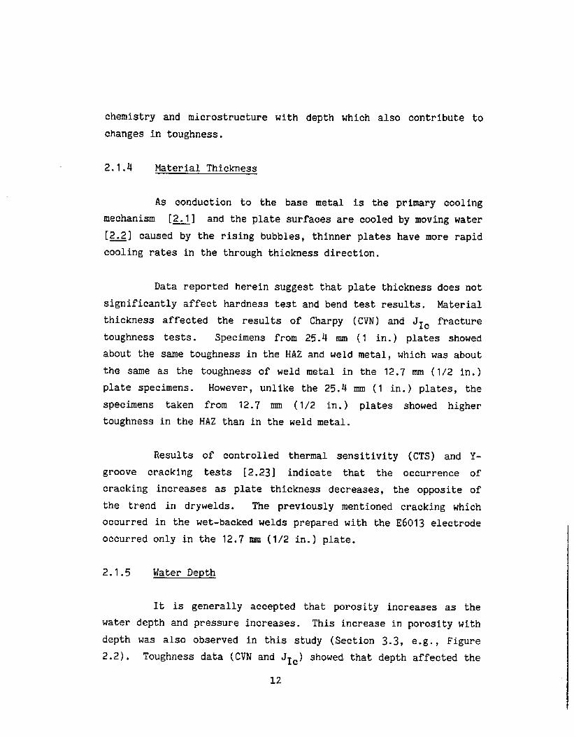
2.1.4 Material Thickness
with depth which also contribute to
As conduction to the base metal is the
mechanism [~] and the plate surfaces are cooled
[2.J] caused
cooling rates
Data
significantly
by the rising bubbles, thinner plates
in the through thickness direction.
primary cooling
by moving water
have more rapid
reported herein suggest that plate thickness does not
affect hardness test and bend test results. Material
thickness affected the results of Charpy (CVN) and JIC fracture
toughness tests. Specimens from 25.4 mm (1 in.) plates showed
about the same toughness in the HAZ and weld metal, which was about
the same as the
plate specimens.
specimens taken
toughness in the
Results
groove cracking
toughness of weld metal in the 12.7 mm (1/2 in.)
However, unlike the 25.4 mm (1 in.) plates, the
from 12.7 mm (1/2 in.) plates showed higher
HAZ than in the weld metal.
of controlled thermal sensitivity (CTS) and Y-
tests [2.23] indicate that the occurrence of
cracking increases as plate thickness decreases, the opposite of
the trend in drywelds. The previously mentioned
occurred in the wet-backed welds prepared with the
occurred only in the 12.7 mm (1/2 in.) plate.
2.1.5 Water Depth
cracking which
E6013 electrode
It is generally accepted that porosity increases as the
water depth and pressure increases. This increase in porosity with
depth was also observed in this study (Section 3.3, e.g., Figure
2.2)* Toughness data (CVN and JIC) showed. that depth affected the
12

weld metal toughness, but HAZ toughness showed inconsistent
results. Bend test results were clearly poorer with increasing
depth. ,
Tests were made in the Gulf of Mexico to determine the
effects of seawater at increasing depths as reported by Grubs and
Seth [2.7]. Four welds were made down to 51 m (166 ft) using E6013
electrodes and the appearance and tensile results were good .
Tensile strength of specimens made from butt welds all exceeded the
minimum for the plate material. Porosity was the only reported
defect. Porosity was rated excessive in the 10 m (33 ft) and 31 m
(102 ft) depth welds and it was noted that the 51 m (166 ft) weld
had an even greater amount of porosity. Porosity was attributed to
the wet electrode coating or waterproofing method used.
2.1.6 Electrode Selection and Welding Position
A wide range of electrodes, both ferritic and austenitic,
have been investigated for metallurgical properties and performance
in underwater welding. Testing has included a variety of coatings
and flux coverings, e.g., cellulose, rutile, oxidizing, and acid
iron oxide and basic types. The rutile ferritic AWS type E6013 is
the most widely applied underwater electrode and is also sold
specifically for underwater welding.
One study [~] found that coatings with iron powder
additions gave the best arc stability where the current and voltage
fluctuations were minimal. A stable cup was provided on the end of
the electrode which appears to provide some degree of mechanical
protection from the water environment. A coating based on iron
oxide gave better resistance to hydrogen cracking which was
attributed to a combination of low-strength weld metal and
beneficial effects of high FeO content on weld metal and HAZ
hydrogen concentrations.
13

The only other alternative found in the study [~] to
reduce hydrogen cracking susceptibility was high nickel or nickel
base deposits. However, austenitic welds contained bands of hard
martensite along the fusion boundaries. High nickel austenitic
welds produced for this same study [2.8] were found to have low
bend test ductility, attributed to grain boundary segregates.
Results reported herein (S”ection 3.4) show the austenitic wet welds
had poorer bend test results than the ferritic welds.
In other tests [2.7], E6013 electrodes were selected
because of better weldability in all positions when used
underwater. Based on the dry weld metal properties E6013
electrodes would not be first choice because of less ductility and
lower radiographic quality than low hydrogen electrodes. However,
low hydrogen electrodes had very poor weldability underwater.
Observations made [2.7] using restraint welding conditions
indicated that the maximum carbon equivalent (CE) without underbead
cracking was 0.392 while the minimum carbon equivalent with
underbead cracking was 0.445. From this study, a “rule of thumbll
was established to use mild steel electrodes for a CE of 0.40 and
lower and for material with a CE of 0.40 and greater austenitic
electrodes should be used. Values recorded for the maximum heat-
affected zone hardness on restrained tests that did not have
underbead cracking were Vickers 30Kg 408 (Rockwell C34). The
minimum heat-affected zone hardness with cracking was Vickers 30Kg
439 (Rockwell C42).
Good tensile test results were reported by Grubbs and Seth
[~] for the E6013 electrodes in spite of the porosity level which
was rated from good to excessive. (The tensile test results
reported herein, Section 3.5, were all greater than the minimum
specified for the base material also despite excessive porosity.)
Porosity was the only discontinuity present in the mild steel welds
14

[~] except for the underbead cracking on the higher
Impact tests conducted on underwater welds compared
indicated the impact strength of the underwater welds
of the strength of the dry weld. However, reasonable
the underwater weld was reported at -l°C (+30°F) with
CE materials.
to dry welds
is about half
toughness for
an average of
30 J (22 ft-lbs) [~]. Results of the present study reported in
Section 3.10 show an average impact energy of 43 J (32 ft-lbs) for
ferritic wet welds compared to 56 J (41 ft-lbs) for dry welds made
with the same electrode.
Testing of austenitic electrodes was made to find suitable
all position welding characteristics that also produce crack-free
welds in the high carbon equivalent materials [~]. Tests made
with the same restraint as for mild steel electrodes on 0.597 CE
material (A-517 25.4 mm (1 in.) plate) demonstrated that high
carbon equivalent material could be successfully wet welded with
high nickel or nickel base electrodes. Results of this study
(Section 3. 10) show an average impact energy of 72 J (53 ft-lbs)
for austenitic wet welds compared to 94 J (69 ft-lbs) for dry welds
made with the same electrode.
Development of a nickel base or austenitic electrode was
conducted for the Naval Facilities Engineering Command [2.9] which
would give deposits having a greater tolerance for hydrogen for
steels of all carbon equivalents. Based on the results obtained in
these tests and other work, the 112 nickel-based electrode and the
R142 stainless steel electrode were recommended. Observations made
on these
undercut
porosity
thickness
results included comments that: welds were free of
and underbead cracking, bead appearance improved and
increased with increasing current, optimum coating
varied with each electrode, depth of cup increased with
increasing coating thickness, proper waterproofing was necessary
for satisfactory operation, and excessive heating damages the
15

waterproof coating even though the coating is not burned completely
by the arc.
2.2 Analysis of Underwater Welding Data Available ~rom theLiterature and from Industry
A statistical analysis was performed of available test
data reported in the literature and gathered for this study from
industry sources. The objectives of this study was to create a
basis for the design of the test matrix. The data were very sparse
(e.g., no JIC or KI~ fracture toughness data was available, only
limited CTOD data was available [2.3] and the only known crack
growth rate data was only recently reported [2.10]). Industry
sources were generally reluctant to release data. Very little data
is available on the long-term performance of underwater wet welded
repairs, because the wet welding technique is widely used only in
the Gulf of Mexico, where inspection requirements are less
stringent, hence many of the repairs have never been reinspected
following completion and acceptance of the work.
A statistical analysis of the experimental data generated
in this program was performed separately and is reported in Section
4. Comparison of the results of these separate analyses is mostly
reserved for Section 4.4. The nature of the test data analyzed in
this section is different than that analyzed in Section 4. The.
data in this section includes a wide variety of materials, test
methods, and test results reported. This data shows only general
effects but is useful because it shows the variability expected for
a wider population of test data. The data analyzed in Section 4 is
for two specific heats of base metal/filler metal combinations, and
tests were conducted under similar and controlled conditions.
Therefore, more significant conclusions can be drawn about the
effect of the variables on these materials, but the results are
1
16

limited to these materials and
generally applicable.
The underwater welding
stepwise regression routine.
cannot therefore be proven to be
data were analyzed using a forward
In this procedure, independent
variables are added one-by-one to a prediction equation on a
dependent variable. The criterion for entering a variable into the
above equation was based on the significance of the partial F test
for the entering variable. If the variable was significant at the
0.25 level, it was included and the stepping procedure continued.
The significance of the estimated coefficients also was determined
using a 0.10 significance level. This was done in order to
discover which variables contributed most to the regression
equation.
The independent variables utilized in the statistical
analyses were:
Wet or wet-backed welding
Carbon or low-alloy steel base plate
Carbon equivalent
Base plate thickness
Carbon steel, stainless, or nickel-base weld metal
DCRP or DCSP (Direct Current Reversed orStandard Polarity)
Flatj vertical, horizontal, or overhead position
Fresh water or salt water
Water temperature
Water depth
Rod or wire diameter.
The dependent variables which were used to examine the
effects of these independent variables were weld metal tensile
17

strength, peak heat-affected zone (HAZ) hardness, bend test (pass
or fail), and nondestructive examination by radiographic (RT)
and/or visual (VT) tests (pass or fail).
Most of the welds in
shielded metal arc weld (SMAW)
data reported for flux core arc
welds (MIG) were also analyzed.
the data base were made by the
process, but a limited amount of
welds (FCAW) and metal inert gas
The contributions of all applicable independent variables
were examined against each of the dependent variables. Subsets
were then selected to eliminate any independent variables which
severely restricted the number of observations because of blanks in
the data base. The evaluations by each dependent variable are
discussed separately in the following paragraphs.
2.2.1 Peak HAZ Hardness
Five independent variables which significantly (90 percent
confidence) explained HAZ hardness were defined as shown in Table
2.1A. The physical effects of two of these, plate steel grade and
water temperature , were rather small (<40 HVN). On the other hand,
wet welding tended to increase the peak HAZ hardness more than 100
HVN compared to water-backed welding, and base metal carbon
equivalent was indicated to increase the peak HAZ hardness
approximately 5 HVN per point (0.01 percent). The prediction
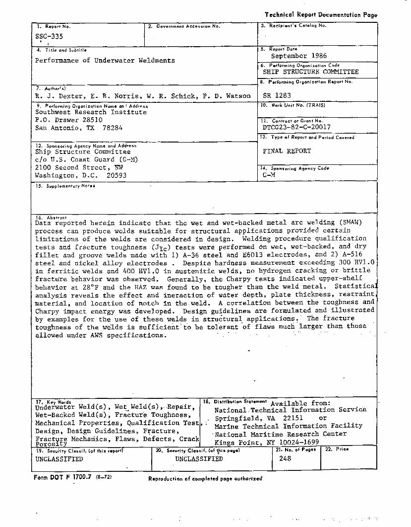
equations for peak Vickers HAZ hardness are:
HVN = 157 + 566(C.E.) for wet-backed welds
HVN = 282 + 566(C.E.) for wet welds
and
18

TABLE 2.1. EFFECT OF WELDING VARIABLES ON HAZ HARDNESS
A. SMAW Only, All CoatinEs --190 Observations
RangeVariables Added (min/max)
Mult. R* Reg.Re~#’a) ( ~ercent) Coeff.
C.E. ( percent) .109/.597Wet 0/1A-36 0/1Thickness (in.)* .375/1.000Water temp. (“F)* 44/80Vertical position 0/1Fresh water 0/1Water depth (ft)* 1/293Electrode dia. (in.)x .125/.188Horizontal position 0/1Flat position 0/1C.S. weld metal -1/1DCRP 0/1
55.557.329.292.203.160.100.670.350.250.760.720.050.02
47.5751.3553.0454.21
55.1355.4455.5555.6355.6955.7155.8855.8955.90
157(b)
566125
-42-45
-1-lo
19<1
282-30-26-1
-2
B. FCAW/MIG Only --44 Observations
(All were wet welds using C.S. weld metal in the flatposition and in fresh water.)
Range Reg.Rem~v~?c) ~~~~c~~t) Coeff.Variables Added (min/max)
760(b)
C.E. ( percent) .180/_.499 64~04 46~10 1638Water temp. (“F)* 60/80 64.71 65.71 14Water depth (ft)* 1/33 26.87 84.16 -7Thickness (in.)* .500/.875 35.68 86.84 -657A-36 0/1 26.28 92.55 195Electrode dia. (in.)x .045/.094 0.18 92.58 95
(a) 90 percent confidence level, F ❑ 2.75(b) Intercept value(c) 90 percent confidence level, F = 2.84* 1.0 in. ❑ 25.4 mm, 1.0 ft = 3048m, (“F-32) 5/9 = “C
19

where (C.E.) = carbon equivalent in percent. The magnitudes of the
contributions of carbon equivalent for wet and wet-backed welds are
illustrated by Figure 2.3.
When two reduced subsets (the top five variables with and
without coating) were evaluated, no other significant variables
were discovered. However, an analysis of the FCAW and MIG data
selected 44 observations, and water temperature, plate thickness,
water depth, and base plate material were indicated to be
additional significant variables for these welding processes (see
Table 2.1-B). It should be pointed out that the 44 observations
were all obtained on wet welds, therefore, no comparative
evaluation could be made between wet and water-backed welds in this
data set.
2.2.2 Weld Metal Tensile Strength
The statistically significant (>90 percent confidence
level) independent variables affecting weld metal tensile strength
were determined to be plate thickness and water depth. The
analysis was repeated using the top five entering variables (plate
thickness, water depth, flat position, base plate material, and
carbon equivalent), both with and without electrode coating as a
sixth variable, to evaluate the latter’s contribution. However,
the number of observations in the six-variable analysis was too
small to provide significant results.
The analysis based on the 13 independent variables
applicable to SMAW welds provided the most useful subset, and the
results are summarized in Table 2.2-A. Again, all of these data
applied to wet welds, so the wet versus water-backed parameter
could not be evaluated. The prediction equation utilizing the two
significant (90 percent confidence) independent variables is:
20

&
600
Wet
500 “
400 “
Wet-Backed
300 ~ 1 I 1●
.30 ● 40 ● 50
Carbon Equivalent, %
FIGURE 2.3. EFFECT OF CARBON EQUIVALENT AND WET VSWET-BACKED WELDING ON HAZ HARDNESS.
21

TABLE 2.2. EFFECT OF WELDING VARIABLES ON WELDMETAL TENSILE STRENGTH
A. SMAW Only, All Coatings --95 Observations
(All were wet welds.)
RangeVariables Added (min/max)
Thickness (in.)~ .375/1.000Flat position 0/1Water depth (ft)* 1/295A-36 0/1C.E. ( percent) .109/.597Water temp. (“F)* 46/85Electrode dia. (in.)* .125/.188DCRP 0/1Horizontal position 0/1Vertical position 0/1
Ft?)Remove a
24.o10.362.852.331.500.960.74o.6g0.070.02
B. FCAW/MIG Only -- 38 Observations
(All were wet welds using C.S. weldposition and in fresh water.)
Range FtVariables Added (min/max) ?)Remove c
Electrode dia. (in.)* .045/.094 2,32C.E. ( percent) .270/.499 1.6oThickness (in.)* .625/.875 0.47Water temp. (“F)* 60/80 0.58Water depth (ft)* 1/33 0.34DCRP 0/1 0.02
(a) 90 percent confidence level, F = 2.79(b) Intercept value(c) 90 ~ercent confidence level, F ❑ 2.88
Mult. R2 Reg.( percent) Coeff.
34:5045.3246.6147.3548.4448.8749.2649.6649.7149.72
54.2(b)41.9
7.2-0.037-5.7
-26.20.2
-123.0-3.0-3.2-1.9
metal in the flat
Mult. R2 Reg.( percent) Coeff.
34.14:62 176.18.61 78.29.76 28.5
10.51 -0.511.42 0.311.47 0.6
* i.o-in-. = 25.4 mm, 1.0 ft = .3048m, (“F-32) 5/9=°C
22
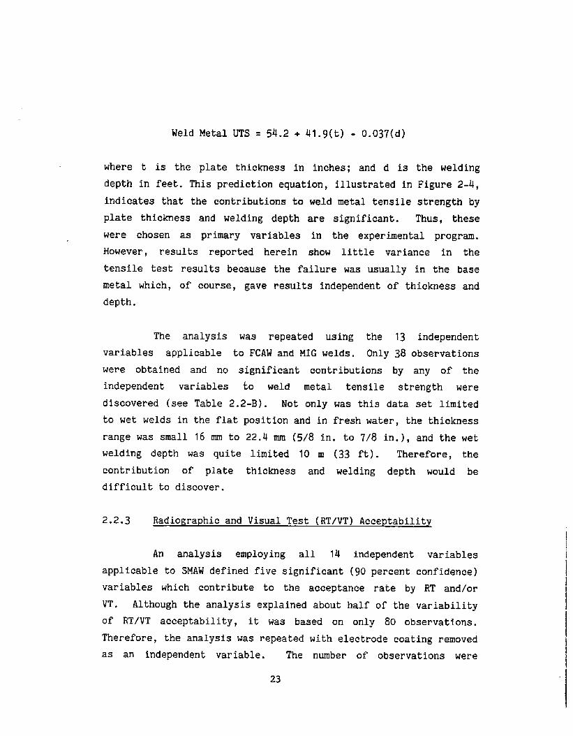
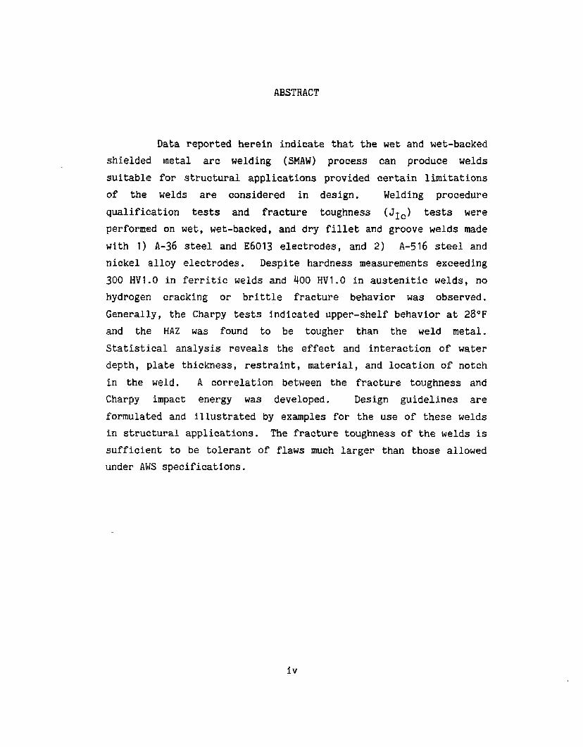
Weld Metal UTS = 54.2+41.9(t) - 0.037(d)
where t is the plate thickness in inches; and d is the welding
depth in feet. This prediction equation, illustrated in Figure 2-4,
indicates that the contributions to weld metal tensile strength by
plate thickness and welding depth are significant. Thus , these
were chosen as primary variables in the experimental program.
However, results reported herein show little variance in the
tensile test results because the failure was usually in the base
metal which, of course, gave results
depth.
The analysis
variables applicable
were obtained and no
independent variables
was repeated
to FCAW and MIG
independent of thickness and
using the 13 independent
welds. Only 38 observations
significant contributions by any of the
to weld metal tensile strength were
discovered (see Table 2.2-B). Not only was this data set limited
to wet welds in the flat
range was small 16 mm to
welding depth was quite
contribution of plate
difficult to discover.
position and in fresh water, the thickness
22.4 mm (5/8 in. to 7/8 in.), and the
limited 10 m (33 ft). Therefore,
thickness and welding depth would
wet
the
be
2.2.3 Radiographic and Visual Test (RT/VT) Acceptability
An analysis employing all 14 independent variables
applicable to SMAW defined five significant (90 percent confidence)
variables which contribute to the acceptance rate by RT and/or
VT. Although the analysis explained about half of the variability
of RT/VT acceptability, it was based on only 80 observations.
Therefore, the analysis was repeated with electrode coating removed
as an independent variable. The number of observations were
23

u
90
80 - (552 MPa)
10 m (33 ft)
70 _ (483 MPa)
60 _ (414 MPa
so (345 MPa)1 1
1/4 (6 mm) 1/2 (13 mm) 3/4 (19”lr011)
Plate Thickness, in.
FIGURE 2.4. EFFECT OF PLATE THICKNESS AND WELDINGDEPTH ON WELD METAL TENSILE STRENGTH.
24

increased to 184, but only one-fourth of the variability was
explained, see Table 2.3. Both analyses indicate that:
● Welds made on A-36 steel base plate tend toproduce less rejects than welds made on low-alloy base plate.
● Increasing carbon equivalent tends to increasethe acceptance rate. This may be confounded bythe electrode selection that could not beincluded in the analysis.
● Warmer water reduces the number of defectivewelds.
● Sounder welds may be produced in thicker plates.
In addition, the 80-observation data set analysis indicates
that increasing the welding depth may decrease the acceptance
rate. Alternately, the 184-observation data set analysis
indicates that fresh water welds may produce less rejects than
salt water welds. Analysis of another subset indicates that
less rejects may be produced when welding in the flat
position.
2.2.4 Bend Test Acceptability
When all 14 independent variables applicable to SMAW
were evaluated against all bend test results, six of the
variables were discovered to be a statistically significant
(9O percent confidence) contributor based on 74 observations,
see Table 2.4-A. Three subsets were evaluated, but the
overall fit appeared to be worse even though more observations
were included. However, since the bend radii varied by nearly
an order of magnitude (1.5t to 10t), the data base was divided
into three groups and reanalyzed.
25

TABLE 2.3. EFFECT OF WELDING VARIABLES ON ACCEPTANCE BY RT/VT
A. SMAW Only -.8o Observations+
.-Range
Variables Added (min/max) Re~o~~a)
A-36 0/1C.E. ( percent) .237/.510Thickness (in.)* .375/1.000Water depth (ft)* 1/295Water temp. (“F)* 46/85Flat position 0/1Rutile coating 0/1Wet 0/1Vertical position 0/1Fresh water 0/1Horizontal position 0/1Electrode dia. (in.) .125/.188
20.808.OO3.256.9o6.540.890.580.330.250.190.050.01
B. SMAW Only, All Coatings--l84 Observations
Mult. R2 Reg.( percent) Coeff.
-1.48(b)
20.23 0.6333.89 2.340.47 0.6044.03 -0.00246.89 0.01248.97 -0.1749.52 0.2049.8g -0.1650.08 -0.09750.26 0.04650.29 -0.04150 ● 30 -0.46
Variables Added
Water temp. (°F)*Fresh waterA-36Thickness (in.)AC.E, ( percent)Flat positionC.S. weld metalWater depth (ft)*WetHorizontal position
Range(min/max)
44;850/10/1
.375/1.000
.109/.5970/1
-1/11/2950/10/1
F toMu t R2 Reg./)Remove a ( percent) Coeff.
O.go(b)5.04 -7.31 -0.0089.33
15.8611.695.912.411.160.590.320.18
13.7817.6721.6223.1525.7326.5026.7526.9026.98
0.310.34
-0.701.3
-0.15-0.04-0.001
0.150.05
Electrode dia. (in.)* .125/.188 0.02 26.99 -0.40
(a) 90 percent confidence level, F ❑ 2.75 ../,
(b) Intercept value(c) 90 percent confidence level, F = 2.79*1.O in. = 25.4 mm, 1.0 ft = .3048 m, (“F-32) 5/9=*c
26. , = -.: ., . .
.... >..-. ...,.... -. .+.W,. ,.. . ..—l.

As an additional independent variable, bend radius was
discovered to be a significant factor, as would be expected, along
with polarity (DCSP is better) and plate thickness (thinner
llaterial is better).
Separate analyses were
subjected to 2t bend tests and 3t
2t bend test group is summarized
carried out on welds that were
bend tests. The analysis of the
in Table 2.4-B; the 3t bend test
group is summarized in Table 2.4-c.
When 2t bend test data were considered separately, weld
metal composition, base metal composition , and water depth emerged
as significant variables, based on 56 observations. An analysis of
the 3t data (79 observations) defined polarity, carbon equivalent
(lower is better) and base plate material (low-alloy steel is
better) as significant variables.
2.3 Conclusions: Factors Chosen for the Test Matrix
Based on the review of the literature and statistical
analysis of available data, the following conclusions were reached:
Weld Type: There is an obvious difference between wet and
wet-backed welds, and since the scope of the project was to include
both types of welds, they were both included in the test matrix.
Dry welds were also included as a basis for comparison. To achieve
consistency, wet, wet-backed welds are normally made with a
different electrode (E7018) than the wet welds (E6013) and the
results for the wet-backed welds made with the E6013 electrode are
not representative of ferritic wet-backed welds in general.
Base Plate Carbon Equivalent and Filler Metal: The
weldability of base plate is related to the amount of carbon and
27

TABLE 2.4. EFFECT OF WELDING VARIABLES ON ACCEPTANCE BY TEND TEST
A. SMAW Only, All Bend Test Diameters -- 74 Observations
Range R to Mult. R2 Reg
Variables Added (min/max) Remove(a) (percent) Coeff.
Water temp. (“F)*Flat positionDCRPRutile CoatingA-36Fresh waterThickness (in.)~Electrode dia. (in.)*C.E. ( percent)Horizontal positionVertical positionWater depth
50~850/10/10/10/10/1
.375/1.000.125/.156.139/.446
0/10/18/295
4:244.05
15.1311.906.583.050.570.640.500.290.030.02
9.4813.7118.4731.5634.3938.1139.9340.4540.9641.3041.3341.35
--3.59(W0.0180.441.61.21.0
-0.610.376.30.720.130.040nil
B. SMAW Only, Bend Test Diameter ~ 2t -- 56 Observations
(All fresh water , no vertical welds.)
Significant RangeRemov~(:?
Multi. R2 Reg.Variables Added (min/max) ( percent) Coeff.
-1.37m
C.S. weld metal -1/1 14.82 13.30 -0.52Water depth 1/293 12.83 22.63 -0.007A-36 0/1 19.74 44.2I 0.88
c. SMAW Only, Bend Test Diameter . 3t -- 79 Observations
(All wet welds.)
Significant. Variables Added
~~:r temp. (OF)*
C.E. ( percent)A-36Fresh water
Range(min/max) Remov~(:y
50/80 1.180/1 6.68
.180/.597 6.130/1 4.150/1 2.61
Multi. R2 Reg.( percent) Coeff.
-2.16(b)
13.26 -0.01019.32 -0.3924.93 -2.530.71 -0.3834.52 0.64
(a) 90 percent confidence level, F ❑ 2.79(b) Intercept value(c) 90 percent confidence level, F ❑ 2.84*1.O in. ❑ 25.4 mm, 1.0 ft = .3048m, (oF-32) 5/9 . oc
28

other elements in
than 0.40 can be
usually requires
cracking. The CE
the steel. Presently mild steels with a CE less
readily welded underwater. Higher CE material
an austenitic filler metal..to prevent hydrogen
influences the hardness of the HAZ. Statistical
analysis showed that increasing the CE decreased the likelihood of
rejection based on NDE, but this is likely to be due to the use of
the austenitic electrodes with these higher CE base plates. Lower
CE base plates performed better in the bend test, but this is also
likely to be influenced by electrode selection.
Small” variation of the carbon equivalent within the range
where ferritic electrodes can be used did not significantly affect
the mechanical properties of test welds [2.3]. Therefore, it was
decided to use a high CE base plate and austenitic filler metal as
well as a mild steel base plate with CE less than 0.40 and a
ferritic filler metal to gather data on these two unique types of
welds. Actual comparison to determine the effect of CE will, of
course, be confounded by the differing filler metal.
Welding Depth: Welding depth influences bead shape and
arc stability as well as the chemistry, microstructure, and
porosity of the weld. It has been shown to affect the occurrence
of cracking (especially under restraint), weld metal tensile
strength, bend test acceptability, and RT/VT acceptability.
Therefore, depth was included in the test matrix. At the time the
test matrix was planned, ferritic wet welds were made down to 60 m
(198 ft), although this capability was recently extended down to
below 100 m (330 ft). Ferritic welds were therefore planned in the
range of 10 m to 60 m (33 to 198 ft) or one to six atmospheres.
Austenitic welds on higher CE base plate are limited to a depth of
about 10 m (33 ft). Originally, the capability to make these welds
down to 60 m (198 ft) was thought to be within reach. However,
attempts to weld at deeper depths failed and the test matrix was
revised to include more ferritic welds instead.
29

Plate Thickness: Plate thickness directly affects the
cooling rate, and hence the hardness and crack susceptibility of
welds. Statistical analysis revealed a possible influence on weld
strength, therefore 12.7 mm and 25.4 mm (1/2 in. and 1 in.) plates
were included in the test matrix.
Other Variables: The above variables were thought to be
the primary factors influencing underwater wet and wet-backed weld
performance. Other variables considered were:
● Polarity: Straight polarity is normally used and
seems to yield better results.
● Water Temperature: Small variations in water
temperature in the range O to 21°C (32 to 70”F)
cannot be shown to contribute significantly to weld
performance.
● Electrode Diameter and Type: Only a few electrode
types and diameters are successfully being used in
wet welding. We chose to use two of the most
commonly used. For one condition in the test matrix,
a weld was made with a larger diameter 4.1 mm (5/32
in.) electrode as well as the 3.3 mm (1/8 in.)
electrode to examine this effect.
● Welding Position: Although the difficulty of welding
is affected by welding position, it could not be
shown to significantly affect hardness, RT/VT
acceptability, weld strength, or bend test
performance, and was therefore not included in the
test matrix.
30

2.4
2.1
2.2
2.3
2.4
2.5
2.6
● Salinity: The performance of welds made in salt
water has been shown to be better than those made in
fresh water [2.22]. Therefore, as a worst case and
for convenience, the test welds were prepared in
fresh water.
References
Brown
Under
June <
Tsai,
R.T., and Masubuchi, K., “Fundamental Research on
Water Welding,tl Welding Journal, Vol. 54, No. 6,
975.
C.L., and Masubuchi, K., “Mechanisms of Rapid
Cooling and Their Design Considerations in Underwater
Welding,” Proceedings Offshore Technology Conference,
Houston, Texas, OTC 3469, April 30 May 3, 1979.
Gooch, T.G., “Properties of Underwater Welds, part 1
Procedural Trials and Part 2 Mechanical Properties,” Metal
Construction, March 1983.
Tsai, C.L., and Masubuchi, K., “Interpretive Report on
Underwater Welding,” Welding Research Council, Bulletin
No. 224, February 1977.
Dadian, M., “Review of Literature on the Weldability
Underwater of Steels,f’ Welding In The World, Vol. 14, No.
3/4, 1976.
Brown, A.J., Staub, J.A., and Masubuchi, K., “Fundamental
Study of Underwater Welding,” 4th Annual Offshore
Technology Conference OTC 1621, April 30 - May 3, 1972.
31

2.7 Grubbs, C.E., and Seth, O.W., “Underwater Wet Welding with
Manual Arc Electrodes,” Published in Underwater Weldi~
for Offshore Installations, The Welding Institute,
Abington Hall, Abington, Cambridge, 1977.
2.8 Stalker, A.W., Hart, P.H.M., and Salter, G.R., “An
Assessment of Shielded Metal Arc Electrodes for the
Underwater Welding of Carbon Manganese Structural Steels,”
Offshore Technology Conference, OTC 2301, Houston, Texas,
May 5-8, 1975.
2.9 Sadowski, E.P., “Underwater Wet Welding Mild Steel with
Nickel Base and Stainless Steel Electrodes,” Welding
Journal, July 30, 1980, pp. 30-38.
2.10 Matlock, D.K., Edwards, G.R., Olson, D.L., and Ibarra, S.,
“An Evaluation of the Fatigue Behavior in Surface,
Habitat, and Underwater Wet Welds,” Underwater Welding
Soudage Sous L’Eau, Proceedings of the International
Conference held at Trondheim, Norway, 27-28 June 1983
under the auspices of the International Institute of
Welding, Pergamon Press, Oxford, England, p. 303, 1983.
2.11 Kobayash, K.,
Proceedings of
London, England,
“Quality Control in Shipbuilding,” in
the International Conference held in
November 19-20, 1975, Vol. 1, The Welding
Institute, Cambridge, p. 28, 1976.
2.12 Newman, R.P., “Effect on Fatigue Strength of Internal
Defects in Welded Joints--A Survey of the Literature,”
BWRA Report D2/2/58, Weld. Res. Abroad, Vol. V, No. 5,
1959.
32

2.13
2.14
2.15
2.16
2.17
2.18
2-.1 g
2.20
Burdekin, F. M., Harrison, J. D., and Young, J. G., “The
Effect of Weld Defects with Special Reference to BWRA
Research,” Weld. Res. Abroad, Vol. 14, No. 7, pp. 58-67,
August-September 1968.
Clough, R., “Application of Weld Performance Data,” ~
Weld. J., Vol. 15, No. 7, pp. 319-325, July 1968.
Pollard, B. and Cover, R.J., “Fatigue of Steel Weldments,”
Weld. J., Vol. 51, No. 11, pp. 544s-554s, 1972.
Honig, E.M., “Effects of Cluster Porosity on the Tensile
Properties of Butt-Weldments in T-1 Steel,” CERL Report
M-109, November 1974.
de Kazinczy, F., “Fatigue
Steel,~l Br. Weld. J.,
Properties of Repair Welded Cast
VO1. 15, No. 9, pp. 447-450,
September 1968.
Carter, C.J., et al., !!Ultrasonic Inspection and Fatigue
Evaluation of Critical Pore Size in Welds,” Technical
Report AMMRC TR-80-35, International Harvester Company,
Hinsdale, IL, AMMRC Contract DAAG46-76-c-0058, September
1982.
Harrison, J.D., “Basis for a Proposed
for Weld Defects”, Metal Construction,
99-107, March 1972.
Acceptance-Standard
VO1. 4, No. 3, pp.
Olson, D.L. and Ibarra, S., “Underwater Welding
Metallurgy” presented at Underwater Welding Workshop,
November 13 and 14, 1985, Colorado School of Mines,
Golden, CO.
33

2.21 Personal communication with J. Dally of Sea-Con Services.
2.22 Grubbs, C.E., “Qualification of Underwater Wet Weld
Procedures at Water Depths Down to 325 Feet” presented at
ADC Diving Symposium, Houston, TX, 1986.
2.23 Masumoto, I., Matsuda, K. and H. Masayoshi “Study on the
Crack Sensitivity of Mild Steel Welded Joint by Underwater
Welding”, Trans. of the Japan Welding Society, Vol. 14,
No. 2, October, 1983.
2.24 Cottrell, C.L.M., “Hardness Equivalent May Lead to a More
Critical Measure of Weldability,” Metal Construction
December, 1984.
34

3.0 EXPERIMENTAL PROGRAM
3.1 The Test Matrix
An experimental program was conducted as part of an effort
to quantify the changes in strength, ductility, and toughness of
wet and wet-backed underwater fillet and groove welds. The test
matrix is shown in Figure 3.1. The experiment was primarily
designed to examine the effect on these properties of:
● Material: A-36 steel with a carbon equivalent
of 0.36 t 0.03 was used with a ferritic filler
metal; and A-516 Grade 70 steel with a carbon
equivalent of 0.46 t 0.03 was used with a nickel
alloy filler metal.
● Plate thickness: For each material combination
above, single bevel groove weld specimens were
prepared from 12.7 mm (1/2 in.) and 25.4 mm
(1 in.) plate thicknesses.
● Depth : Ferritic wet welds of 12.7 mm (1/2 in.)
and 25.4 mm (1 in.) thickness were prepared at
60, 35, and 10 m (198, 115, and 33 ft); as well
as dry welds prepared at the surface. 25.4 mm
(1 in.) thick ferritic welds were also made at
20 and 30 m (66 and 99 ft). Wet-backed welds
are prepared only at 10 m (33 ft). Austenitic
wet and wet backed welds were also prepared at a
depth of 10 m (33 ft) as well as dry welds.
35

FIGURI 3.1. TEST MATRIX
Note: 1/2 in. = 12.7 mm1 ill. = 25.4 mm1 ft = .3048 m

Other plates were prepared to examine:
● Restraint: A series of 25.4 mm (1 in.) thick A-
36 groove weld plate specimens were prepared
from plates pre-welded to a very stiff frame,
simulating restrained structural joints.
● Weld Preparation: A double bevel weld was
prepared at 10 m (33 ft) for the 25.4 mm (1 in.)
ferritic weld. All other welds in the study
were single bevel preparations.
● Procedure Variation: An additional 25.4 mm (1
in.) ferritic single bevel weld was made with a
procedure variation, specifically a 4.1 mm (5/32
in.) electrode was used rather than the standard
3.3 mm (1/8 in.) electrode.
● Fillet welds: A set of fillet weld tensile
tests and fillet weld break-over tests will be
conducted on ferritic fillet welds prepared at
three depths from 12.7 mm (1/2 in.) material.
● Weld metal tensile strength: Extra width 25.4
mm (1 in.) thick groove welds are prepared to
extract all-weld-metal tensile test specimens.
The austenitic welds at 35 and 60 m (115 and 198 ft) depth
were originally planned, however, these welds could not be made and
were dropped from the test
the matrix are hatched.
the additional 25.4 mm (1
20 and 30 m (66 and 99
procedure and preparation
matrix. In Figure 3.1 these sectors of
Instead of the deeper austenitic welds,
in.) ferritic welds were made; welds at
ft) and welds at 10 m (33 ft) using a
variation. With these additions, better
information about the variation of weld quality and toughness can
be obtained by concentrating tests at 10 m (33 ft). Also the
37
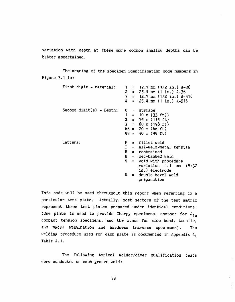
variation with depth at these more common shallow depths can be
better ascertained.
The meaning of the specimen identification code numbers in
Figure 3.1 is:
First digit - Material: 1 = 12.7 mm (1/2 in.) A-36= 25.4MM (1 in.) A-36
S ❑ 12.7MM (1/2 in.) A-5164 = 25.4MM (1 in.) A-516
Second digit(s) - Depth: O = surface1 = 10m (33ft))2= 35m(l15ft)3= 60m (198ft)66 ❑ 20m (66 ft)99 = 30m (99 ft)
Letters: F = fillet weldT= all-weld-metal tensileR= restrainedB = wet-backed welds= weld with procedure
variation 4.1 mm (5/32in.) electrode
D = double bevel weldpreparation
This code will be used throughout this report when referring to a
particular test plate. Actually, most sectors of the test matrix
represent three test plates prepared under identical conditions.
(One plate is used to provide Charpy specimens, another for JIC
compact tension specimens, and the other for side bend, tensile,
and macro examination and hardness traverse specimens). The
welding procedure used for each plate is documented in Appendix A,
Table Al.
The following typical welder/diver qualification tests
were conducted on each groove weld:
38
i

1. Visual examination
2. Radiographic examinations
3* Bend tests at 57.2 mm (2.25 in.) radius, 25.4 mm (1in.) radius , and 19.0 mm (0.75 in.) radius
4. Reduced section (transverse weld) tensile tests
5. Metallographic macro examination
6. Hardness traverse
All-weld-metal tensile tests were performed on specially
prepared ferritic groove welds at 10, 3S and 60 m (33, 115, and
60m (lg8 ft). Chemical analysis of the base metal and filler
metals was also performed. Charpy V-notch impact tests and J1c/-
CTOD fracture mechanics tests were conducted for both the weld
metal and heat affected zone locations of all the welds. The
purpose of the JIC tests is to make comparisons of fracture
toughness among the welds and to establish the ability of the
Charpy test to predict the fracture toughness. For most groove
welds, only two JIC tests were performed, one precracked in the
heat affected zone (HAZ) and one precracked in the weld metal.
The fillet weld specimens are tested for ductility in a
break-over bend test and for shear strength in a fillet weld
tensile test. Comparisons are made of the shear strength of these
fillet welds to the tensile strength obtained from all-weld-metal
tensile specimens prepared from the same filler metal at the same
depth .
Section 3.2 presents a discussion of findings from the
experimental program, excluding the statistical analysis which is
presented in Section 4.0. Detailed descriptions of the test
procedures and results are presented in Appendix A.
3.2 Discussion of Test Results
39

3.2.1
parallel
Visual and Radiographic Examination
Wet-welded plates were generally found to have two
grooves along each fusion line at the weld root
(inadequate joint penetration). Radiography revealed the porosity
in the wet-welds, and slag inclusions in a few plates. A crack was
found in the 12.7 mm (1/2 in.) ferritic wet-backed weld llB-2. The
ferritic wet backed welds were purposefully made with a poor choice
of electrode for wet-backed welding. Wet-backed welds are usually
made with an E7018 electrode. However, the same E6013 electrode
that was used for the wet welds was also used for these wet-backed
welds in order to have consistency in the test matrix. Results
from these ferritic wet-backed welds cannot be thought of as
typical for wet or wet-backed welds. Note that it is possible the
poor results obtained for the wet-backed weld could possibly be
affected by the waterproof coating used on the E6013 electrode,
which was not intended to be used in the dry.
The order and/or spacing of the specimens was in four
cases rearranged to avoid defects detected from radiography. Since
there is an extra bend specimen provided, the defect was generally
isolated in a single bend specimen. The following plates were the
only plates purposefully rearranged to avoid defects:
llB-1 tens ile and bend specimens were
rearranged to get tensile specimens
away from a large crack.
11-1 tensile and bend specimens were
rearranged to isolate a slag
inclusion approximately 12.7 mm (1/2
in.) long slag in several bend
specimens.
40

20-2 tensile and bend specimens were
rearranged to isolate a slag
inclusion approximately 9.5 mm (3/8
in.) long in a bend specimen.
21-T-2 all-weld-metal tensile specimen loca-
tion was chosen to avoid two slag
inclusions in the gage length.
In all other plates, it was not deemed advantageous
specimens, i.e. either the discontinuities were small
to rearrange
and would be
typical of Type B welds or they were prevalent throughout the weld,
e.g. porosity. The significance of the limited rearranging that
was done is not thought to be great, since many discontinuities
were discovered in test specimens after sawing or testing which
were not evident from the NDE. Note also that 1) plate llB is a
wet-backed weld made with an improper electrode, and the results of
these wet-backed welds are of questionable use anyway, 2) plate 20
is a dry weld, and 3) plate 21-T is used only for
metal specimen. Therefore, only one wet welded plate
for test specimens and this could not significantly
results of this program.
the all-weld-
was rearranged
bias the test
Normally a plate would be rejected on the basis of the
radiographic indication. In view of the use of this data for
application in design rules, it was decided to proceed with testing
of these plates. Once a welding procedure is qualified under the
AWS D3.6 specification for Type B welds, subsequent production
underwater welds prepared with this qualified procedure would
probably be subjected to less scrutiny than the welds used in these
tests. Hence, the number and size of these defects in the test
welds are probably less than those of actual service welds.
41

3.2.2 Side Bend Tests
Side bend tests were performed as part of the typic~l
qualification tests as outlined in AWS D3.6 Specification.
weld
The
test gages the ability of the weld to deform plastically as it is
bent 1800 at a specified radius. The specification requires that
for Type B welds, four side bend test specimens be bent to a radius
of six times the 9.5 mm (3/8 in.) specimen thickness (6T) or 57.2
mm (2.25 in.). In addition, for the purposes of this project,
specimens are bent to selected smaller radii so that it can not
only be determined if the weld qualifies as a Type B weld, but also
just how much additional ductility is afforded by the welds.
Actually, to qualify as a Type A weld, four side bend tests should
be bent to a (2T) or 19 mm (3/4 in.) radius. We have indicated
several weldments that appear to be able to meet this requirement
of Type A welds, although because of a limited number of specimens,
only two or three specimens were bent to the (2T) or 19 mm (3/4
in.) radius.
The results of the bend tests are summarized in Table 3.1
in the form of a relative score based on the best performance being
equal to 100. The weld type shown in Table 3.1 indicates that only
the results of the bend test satisfy the requirements of that weld
type, i.e. other requirements may not be satisfied. In addition,
because only a limited number of specimens were available and most
were used at larger radii, those welds indicated to have passed the
Type A bend test requirements did not always pass four tests.
Strict interpretation of the AWS D3.6 Specification
indicated that if any of the first four 6T 57.2 mm (2.25 in.) bend
tests fail to meet the requirements (i.e.,
3.3 mm (1/8 in.)), the procedure is not
weld. By this strict interpretation,
42
cracks must be less than
qualified as a Type B
the 12.7 mm (1/2 in.)
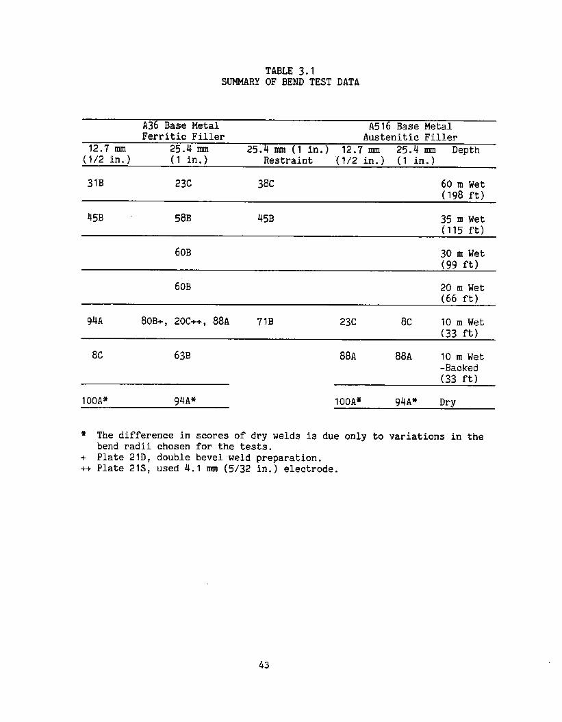
TABLE 3.1SUMMARY OF BEND TEST DATA
A36 Base Metal A516 Base MetalFerritic Filler Austenitic Filler
12.7 mm 25.4 mm 25.4 mm (1 in.) 12.7mm 25.4 mm Derth(1/2 in.) (1 in.) Restraint “ “(1/2 in.) (1 in.) ‘
31B 23C 38c 60 m Wet(198 ft)
45B 58B 45B 35 mWet(115 ft)
60B 30 m Wet
60B 20 m Wet(66 ft)
94A 80B+, 20C++, 88A 71B 23c 8C 10 mWet
8C 63B 88A 88A 10 m Wet-Backed
(33 ft)
10OAS 94A* 100A* 94A* Dry
* The difference in scores of dry welds is due only to variations in thebend radii chosen for the tests.
+ Plate 21D, double bevel weld preparation.++ Plate 21S, used 4.1 mm (5/32 in.) electrode.
43

ferritic wet-back weld, a ferritic wet weld prepared at 10 m (33
ft) with a 4.1 mm (5/32 in. ) electrode as an intentional procedure
variation, both austenitic wet welds, and the 25.4 mm (1 in.)
ferritic wet welds from 60 m (198 ft) depth (both with and without
restraint) do not qualify as Type B welds. The 25.4 mm (1 in.)
ferritic wet welds from 60 m (198 ft) were clearly very close to
the borderline of Type C to Type B classification according to bend
test criteria. Specificallyj four out of five 6T bends for the
25.4 mm (1 in.) unrestrained ferritic wet weld at 60 m (198 ft),
(23-3) and six out of seven for the same weld restrained (23 R-1 )
did pass. The results of tests on these ferritic welds from 60 m
(198 ft)
group of
depth were therefore conservatively considered among the
Type B welds.
The austenitic wet welds did not qualify as Type B welds
according to bend test criteria; e.g., 6 out of 8 6T bends passed
for the 12.7 mm (1/2 in.) weld and 4 out of 7 for the 25.4 mm (1
in.) weld. It is interesting to note that although the austenitic
wet-welds exhibited poor bend test results, these welds have very
good fracture toughness. These bend tests failed because pores
opened up to greater than 3.3 mm (1/8 in.) although they were bent
fully 180°. The present requirement of AWS D3.6 is a good
screening test for weld workmanship, but should not be regarded as
indicative of the total ductile capacity to rotate (i.e. only the
capacity to rotate up to par elongation is indicated) or toughness.
The failure of the 12.7 mtn (1/2 in.)ferritic wet-backed
weld must be considered along with the fact that these welds were
prepared with an improper electrode, E6013. The 25.4 mm (1 in.)
ferritic wet-backed weld passed all the 6T bend tests; however, one
of the bend specimens (which remains untested) contains
would obviously fail if tested. A 2T and 2.67T bend
for this weld, indicating the ductility is quite good.
44
a crack and
also passed
Therefore,

the 25.4 mm (1 in. ) ferritic wet-backed weld was still classed as
Type B with respect to bend test criteria, not withstanding the
obvious cracking problem that was caused by intentional use of an
improper electrode.
3.2.3 Transverse-Weld Tension Test
The transverse-weld reduced-section tensile tests all
passed the requirements for Type A welds (identical to the
requirements for Type B welds). Most (76 percent) of the specimens
fractured in the base metal, with the tendency to fracture in the
weld increasing with depth (and porosity). Those specimens which
fracture in the weld metal exhibited very little elongation. The
transverse weld tension test reveals very little about the
performance of the weld other than assuring adequate strength and
fusion, which can be assured by the bend test. More useful
information can be obtained from an all-weld-metal tension test,
e.g. weld metal yield , ultimate, and elongation.
3.2.4 Hardness Traverse
Small portions of the heat-affected zone (HAZ), usually
found near the weld crown, had Vickers hardness (HV1.0) of up to
334 for the wet ferritic welds and up to 46o HV for the austenitic
wet welds. Nearby impressions (within 0.5 mm (.008 in.)) were
often 200 HV less hard, indicating the high hardness” was a very
localized phenomenon. This spatial variability on a single
specimen explains the wide scatter in hardness measurements both
for a single specimen and between specimens. Dry and wet-backed
welds were not nearly as hard. In the statistical analysis in
section 4.0 it is shown that hardness is generally independent of
depth and cannot be correlated to toughness or performance in the
bend test. Because of the absence of cracking or brittle fracture
45

behavior in all the wet welds, the hardness of the weld seems
insignificant.
3.2.5 Fillet Weld Tests
Fillet weld break-over bend tests and fillet weld tensile
tests were conducted and the results of these tests would qualify
these fillet welds as Type B. The fillet weld bend specimens
failed before being bent to 45”, but failed in the throat
exhibiting good fusion and lack of obvious defects.
The failures of the fillet weld tensile tests were all
remarkably ductile, i.e. the plates extended (slid apart)
appreciably before breaking. The results from pairs of these tests
were as follows:
● llF: Shear(6o percent
● 12F: Shear(6o percent
● 13F: Shear(6o percent
strength = 373 and 337 MPa (54.1 and 48AWM tensile strength = 47.6 ksi)
strength = 379 and 338 MPa (54.9 and 49AWM tensile strength = 281 MPa(40.7 ksi,
strength = 322 and 310MPa (46.7 and 45.AWM tensile strength = 271 MPa (39.3 ksi)
9 ksi)
O ksi)
O ksi)
Sixty percent of the specified minimum tensile strength
(400 MPa (58 ksi)) of the A-36 base material is 24o MPa (34.8 ksi),
. and since the shear strength is larger the welds are qualified as
Type B fillet welds. They also meet the more stringent
requirements for a Type A fillet weld (6o percent of the average of
the all-weld-metal ultimate tensile strength) which is also
reported above.
3.2.6 All-Weld-Metal Tensile Tests
All-weld-metal tensile tests
46
were conducted on the ferritic

wet-welds although these tests are not required for Type B
qualification. The tests revealed the weld metal has the required
strength, although elongation was insufficient to qualify the welds
as Type A. The results are summarized in Table 3.2.
3.2.7 Charp y Tests
Charpy impact tests are often used to indirectly estimate
the fracture toughness of metals. This practice is less desirable
than direct measurement of toughness with KIC, JIC or CTOD tests.
However, due to the relative difficulty and expense of the latter,
the Charpy test will probably continue to be used. Therefore, as
part of our investigation, we will investigate the correlation
between Charpy impact toughness and JIC or KIC, as well as
investigate the trends in impact energy and toughness among the
variables of this experimental program.
Charpy tests were conducted at -2° and 160c (28° and 60°F)
for all weldments. The impact energy for the ferritic weld metal
was low (typically 20-47 J (15-35 ft-lbs)) with the exception of
the dry welds. For the 12.7 mm (1/2 in.) ferritic welds, HAZ*
impact energy 54-76 J (40-56 ft-lbs) was higher than the weld metal
impact energy. For the 25.4 mm (1 in.) ferritic wet welds, the HAZ
impact energy 9-15 J (7-11 ft-lbs) was lower than the weld impact
energy. The impact,energy for the austenitic welds was much higher,
ranging from 45 to 155 J (33 to 114 ft-lbs).
Most of the conditions tested indicate “upper shelf” or
full shear behavior at 28°F. Specimens which did not exhibit full
shear behavior include both thicknesses of the dry and wet-backed
*The notch for these HAZ Charpy tests was located about 1 mm fromthe fusion line, see the Appendix Section A.9.
47

TABLE 3.2
SUMMARYOF ALL-WELD-METAL TENSILE TESTS(25.4mm (1 in.) Thick A-36 Plate, Ferritic Filler)
Proportional Yield TensileLimit Point Strength Elongation
(MPa) ks i (MPa) ks i (MPa) ks i (%)
60 m 350 50.8 402 58.4 451 65.5 9.4(198 ft) 350 50.8 402 58.4 451 65.5 9.4
35 m 384 55.8 437 63.5 475 69.0 6.3(115 ft) 395 57.4 423 61.4 458 66.5 6.3
10 m 472 68.5 507 73.6 556 80.7 12.5(33 ft) 464 67.3 493 71.6 539 78.2 9.4
48

E6013 weld metal, the 25.4 mm (1 in.) ferritic HAZ’S, and the 25.4
mm (1 in.) dry austenitic HAZ.
If the Charpy tests exhibit upper shelf behavior at this
temperature, then the more slowly loaded JIC fracture toughness,
and the fracture toughness exhibited by the welds in the structure
will also be expected to be upper shelf at this temperature.
Therefore ductile tearing rather than brittle fracture would
generally be anticipated in structures with underwater welds with
the following exception. As pointed out above, the HAZ of 25.4 mm
(1 in.) thick and thicker is in the transition or lower shelf
region of the Charpy toughness vs temperature curve at 28o. The
fracture of structures welded with 1 in. thick and thicker plates
with the ferritic electrode cannot be generally assured to be
ductile above -2°C (28°F) but may depend on strain rate,
temperature and constant. Ductile tearing allows load to
redistribute and in a redundant structure, considerable stable
tearing can probably be accommodated without complete separation of
the component.
Although there was some considerable scatter in the Charpy
data, as the ranges above show, the toughness within any category
of weld and in a particular location (HAZ or weld) varied in a
fairly narrow range. The variance exhibited for austenitic welds
is primarily due to several exceptionally tough samples. The
Charpy test often exhibits a great deal of scatter even for
homogeneous base metals. This scatter is partly due to the fact
that the Charpy specimen samples only a small volume of material.
This localized variation of material properties, as was noted for
the hardness test results, is more apprent in the results of a
Charpy test then a tensile test, for example.
49

3.2.8 JIP Fracture Toughness Tests
Tests were conducted to determine the fracture toughness of
the weld and heat affected zone. The test selected for this
purpose was ASTM E813 “J ~C, a Measure of Fracture Toughness”. This
test is more appropriate than ASTM E399 (KIC) “Plane-Strain
Fracture Toughness” for ductile materials. The KIC toughness can
still be determined by JIC = K1c2/E. For
data was reduced such that the crack
(CTOD) could also be determined.
The value of KIC determined from
to be generally conservative [~1. This
different point of measurement inherent
“several of the tests, the
tip opening displacement
this test has been shown
is chiefly because of the
in the test methods E813
(JIC) and E399 (KIC); i.e., the measurement of JIC is taken at a
point where the R-curve intersects the “blunting line” given by:
J = 2 uflowAa.
The total crack growth, Aa, at this intersection, theoretically the
point of initial actual crack advance, is generally much smaller
than the 2 percent offset of the crack length used as a measurement
point for KIC in ASTM E399. Thus, for steels which fracture by a
ductile mode, JIC represents a lower bound to KIC.
Figure 3.2 shows a typical load vs load line (clip gage)
displacement trace for a J1c/CTOD test of a 25.4 mm (1 in.)
ferritic weld metal mode at 10 m (33 ft). Partial unloading were
performed to obtain the crack length by compliance. J is
calculated from the area under the curve, and CTOD is calculated
from the clip gage displacement. Figure 3.3 shows the J-resistance
curve. The line to the left is the blunting line. Note the clear
50
,..

I I 1 I I\
I I I I
.-., .,. . . . . . . . . . . . . -,, < . . . . . . . . . . . . . . . , . . .
. . . . . . . . . . .,, ,, ... .+ “. . . . . . . .
. .
. . . . . . .,1-Ln
. . . . . . .
. . . . . . . . . . . . . . . . . . . .
IA1-
. . . . . . ., . . . . . . . . . . . .
. . .
,.. .
. . . . . . . . . . . . . . .. . . . . . .,t?
U-Jml
, . . . . .
. . . .
. .
. . . . . . . . ‘Ei<’”:. . . . . . . . . .. . . . .. . . . . . .
.,
. . . . . . . . . . . . . . . . .
‘L< ~k........---i-””-”+ ““””
b:,- ;.....,J-” ””:.””-””;:””””.-,Ae : :
..........-
.........., —. .........:.....,,”
1
- .,Ei-a . .
. .
. . .
. . . . . . . . . . ..
...“
II II
00. .
51

O.lyj
e.
. . . .
. . . .
. . . .
. . . . .
.,.
,,-
-,
. . . . . . . ..
. . .
. . .
. . . .
. . . .
. . . .
1’
. .
. . . .
. .
. .
-,. .
. . . . . .
. . . . . .,+.
. . . . . ..%+
M-
. . .
,..
:E
F.:,.A.x
. . . . . . . . . .
. . . . . . . . .
I
. . .
.,
.
. .
. .
. . .
.x
. . .
. . .
,.FIGURE 3.3 EXAMPLE OF J ‘IUZSISTAI?CE CURVE
1.0 in lb = .175 ~
in2‘2
m
1.0 in. = 25.4 mm
“52;

break in slope as the initiation of tearing occurs. ‘Ic for this
specimen was 91 kJ/m2 (522 in~lb/in.2), KIC derived from JIC was
135 MPa#~ (123 ksi/~).
For failure to occur by ductile tearing in the structure,
two criteria must be satisfied: 1) the applied J (from structural
analysis) must exceed JIC and 2) the rate of change of the applied
J with respect to crack extension must exceed the rate of change of
the J-resistance curve with respect to crack extension, i.e. the J
applied must remain above the J-resistance. The slope of the J
resistance curve is therefore also an important material property
and has been given the name “tearing modulus” or T’.
L
The slope of the curve is normalized by the modulus over the flow
stress squared because it is dimensionless and this is how the term
appears in a structural analysis. If, for example, a crack in the
structure is loaded such that J exceeds JIC but the applied T is
less than T-resistance, only a limited amount of tearing will occur
(until J-resistance exceeds J-applied) and the structure will
remain stable. Thus a great deal more resistance to fracture is
afforded by these welds than is evident by JIC or KIC derived from
JIC.
The CTOD also increases in a stable manner with crack
extension. Figure 3.4 shows the CTOD vs. crack extension for this
weld and a resistance curve construction similar to that for JIC
determination. Here the blunting line is given by:
CTOD = 2Aa
53

1 II 1-
. . . . . . . . . . . . . ..-. . . . .. . . ., . . . . .
. . . . .
.,
“l””rlI
1
.1
r
1 [
,. ...%. . . . . . . .
c
. . .
. . .
. . .
i/I
,.. . ..+
r-l---. . . . . . . . . . . . . . ..-
. . . . . . . . . . . . .!
. . . . . . .
. . . . . . .
... ,.. . . . . . . . .
. . . . . -. . . . . . .
II
71
CURVEFIGURE 3.4. EXAM?LE OF CTOD P2LSISTANCE
= 25.4 mm1.0 in.
.34

Theoretically, J is equal to the flow stress times CTOD, and the
above expression for the blunting line for J is based on the simple
assumption that the apparent crack extension will be one half the
CTOD. Again, this analysis works very well for there is a clear
break in slope at the initiation of tearing. The point of
intersection of the regression line of points between offsets of
0.15 and 1.52 mm (0.006 and 0.06 in.) from the blunting line with
the blunting line is designated as the initiation value of CTOD, or
CTODi . CTODi for this case was 0.12 mm (0.0048 in.) In the
British Standard for CTOD testing, BS 5762 [3.4], there is no
definition of CTODi. Rather, to simplify the test and not require
compliance crack length measurements, CTOD is taken as the value at
maximum load. In Figure 3.4 this point is labelled “max” and has a
value of 0.13 mm (.0052 in.) Experience in this type of testing
indicates that there is much more scatter in the maximum load value
and there is also some thickness and specimen dependence which is
not observed for the CTODi. Therefore, the more conservative value
of CTODi is recommended.
J and CTOD are theoretically related
J = n Uf CTOD
where q is a factor greater than but nearly
by the expression
equal to 1 and depends
on the constraint in the specimen and hardening of the material.
Figure 3.5 shows a plot of J vs CTOD multiplied by flow stress
where J and CTOD were measured independently. From Figure 3.5 it
is seen that the value of n is about 1.5 for the 25.4 mm (1 in.)
thick specimen. Similar results show n is about 1.7 for the 12.7
mm (1/2 in.) thick specimens.
The bars in Figure 3.6 show JIC and are grouped according
to the depth of the weld preparation. Figure 3.6 shows the
55

.
.
----
-.
. . . .
. .
,.
. . . . .
. . . . .
. .
,.
,.
.
. . . . .
. . . .
. . . . . .
,.. . . . .
. . . .
. . . . . .
.
. .
. . . .
. . .
. . .
,. ...
. . . . . . .
. . . . . ,4. . .
. ...<
. .
,..
,
. .
.,
.-. .. . . . ..- . . . . . . . . . ~
. . . . . . . . . . . . . . -.. . . . . . . . . . . . . . . . . . . .. . . . . . . . . . . . . . . . .
. . . . . .. .
. . . . . . . . . . . . . . . . . . . .
‘J
. . . . . . . .
in-lbs1.0 ~ = 0.175 ~
in m
FIGURE 3.5 EXAITFLE OF RELATIONSHIP BETWEEN J AND CTOD

EitiHJ
1 %............... ,..,,.:,:i..:.;?......... -.
t-m-l-l
II
au-l
57
. ..> .

relatively
welds in
austenitic
than their
high toughness of the wet-backed and dry austenitic
both the weld metal and heat-affected zone. The
wet welds at 10 m (33 ft) are not significantly better
ferritic counterparts.
Restraint does not seem to significantly influence the
fracture toughness, although the restrained welds consistently
performed slightly worse than the unrestrained equivalent welds in
both weld metal and heat-affected zone.
With two significant exceptions 25.4 mm (1 in.) ferritic
air weld and 25.4 mm (1 in.) austenitic wet-back weld, the heat-
affected zone toughness was generally greater than or about the
same as the weld-metal toughness. This may simplify any
application of this study to design guidelines.
Figure 3.7 shows the value obtained for KIC plotted with
the upper shelf Charpy impact energy. Also shown on the figure is
the Rolfe-Novak correlation for upper shelf KIC and CVN [~]:
Here u is the yield stress in ksix and the two lines correspond
to uys!~6 (base-metal yield strength) and uys =, 60 (average yield
strength of the weld metals). KIC in this relation is in ksiiin.
and CVN is the upper shelf Charpy impact energy in ft-lbs.*
Note that for some HAZ specimens of the 25.4 mm (1 in.)
thick ferritic weldments the Rolfe-Novak correlation would yield
~1.O ksi=6.895 MPa, 1.0 ksi~.=1.l MPafi, 1.0 ft-lb=l~356 J
58

C4
.
-4
:’59

unconservative estimates of KIC. However, for these 25.4 mm
(1 in.) thick ferritic HAZ specimens, the Charpy test did not
exhibit upper shelf results at -2°C (280F), and the JIC results
“non-upper-shelf”.could also be Therefore, the Rolfe-Novak
correlation is not applicable to these points. The points with
very high KIC for which the Rolfe-Novak correlation is overly
conservative are for the most part austenitic welds, for which the
correlation, which was developed for ferritic materials, is also
not applicable. Finally, the one result at 30 J (22 ft-lbs) for
which KIC is only 33 MPa/~ (30 ksi~~.) is probably a special
case. The JIC curve for this case exhibited virtually no blunting
and was probably in the vicinity of a gross defect. The tearing
modulus for this specimen (12-2-lW) was about the same as the
tearing modulus for the weld metal specimen at 60 m (198 ft) (13-3-
lW). ‘et ‘Ic for the ferritic weld metal at 60 m (198 ft) was much
higher, i.e. 85 MPa /~ (77 ksi/~). Because the trend is
decreasing toughness with increasing depth, one would expect the
toughness at 35 m (115 ft) to exceed 85 MPa/~ (77 ksi l=.).
There appears to be less scatter among the weld-metal
results than among the heat-affected zone specimens. Therefore,
there may be a better correlation for the weld-metal toughness.
JIC tests indicated great variability in toughness smong
the welds tested. JIC ranged from 4.9 to 565 kJ/m2 (28 to 3231.
in.-lb/in.2 and corresponding KIC (calculated from JIC) ranged from
33 to 353 MPa/fi (30 to 321 ksi/fi.). Austenitic welds were
generally tougher than the ferritic welds and the minimum KIC was
45 MPa#~ (41 ksi/~.). Excluding the special case discussed above,
the minimum JIC was 9.5 kJ/m2 (54 in-lb/in2). The HAZ toughness
was generally greater than the weld metal toughness. Toughness
seemed to decrease with depth, with the exception of the 12.7 mm
(1/2 in.) ferritic HAZ specimens.
60
3.2.9 Chemical Analyses
Chemical analysis was performed on
base metals, a sample of the ferritic weld
both thicknesses of the
metal made at 60 m (198
ft), and a sample of the austenitic weld metal mode in a wet-backed
weld. At the time, it wasn’t realized that the weld metals
chemistry might change with depth. In retrospect, it would better
to have samples of the weld metal from all depths, dry, and wet-
backed welds.
Table 3.3 shows the results of these chemical analyses.
Note the particularly low mangense in the ferritic weld at 60 m
(198 ft). This percentage is probably much lower than would be
obtained in a dry weld and is consistent with the results of Ibarra
and Olson discussed in Section 2.
61

TABLE 3.3
CHEMICAL ANALYSIS
(percent by weight)
Plate Sample c MNSiPS Ni Cr Mo Cu V CE
(13) 1/2 in.A-36 (12.7 rmn) .17 .87 .26 .014 .016
(26) 1 in.A-36 (25.4 mm) .14 .86 .23 .033 .023
(23) E6013welded at198 ft (60m) .09 .32 .22 .020 .010
(31) 1/2 in.A-516 (12.7 MM) .22 1.04 .20 .018 .015
(41B) 1 in.A-516 (25.4 mm) .22 1.07 .21 .024 .011
(41B)Austenitic
J-J1* .O1* .O1* .01 .o1* .32
.09 .02 .O1* .04 .01 .30
.02 JJ1* .O1* *O1 .01
.O1* .02 .O1* .01 .O1* .40
.01 .02 .O1* .01 ●01* .41
Wet-Backed .05 2.03 .34 .008 .012 62.72 12.52 5.61 .02
*Less than or equal to
62

3.3 References
3.1. Landes, J.D., and Begley, J.A., “Recent Development in JIC
Testing,” Development in Fracture Mechanics Test Methods
Standardization, ASTM STP 63z, 1977, pp. 57-81.
3.2. Landes, J.D., and Begley, J.A., in Fracture Analysis, ASTM
STP 560, 1974, pp. 170-186.
3*3. Rolfe, S.T., and Novak, S.R., “Slow-Bend KIC Testing of
Medium Strength High-Toughness Steels,!’ ASTM STP 463,
1970, pp. 124-159.
3.4 British Standards Institute BS5762 “Methods for Crack
Opening Displacement (COD) Testing”.
63

4.0 STATISTICAL ANALYSIS OF TEST DATA
4.1.1 Decomposition of The Test Matrix
Statistical analysis was performed for the overall test
matrix shown in Figure 4.1 which identifies the test welds from
which specimens for bend tests, transverse weld tension tests,
Charpy impact tests, hardness traverse, and JIC fracture toughness
tests have been taken. Not shown in this test matrix are the
fillet weld tests and all-weld-metal tension tests, which are
analyzed separately.
The test matrix can be considered in total and as the
combination of three separate subgroups within which some of the
test variables are removed. These subgroups are shown in Figure
4.2.
The Restraint Subgroup allows a one-to-one comparison of
25.4 mm (1 in.) A36 base plate welded with and without restraint of
the plates during welding and cooling. Since restraint can cause
cracking from the shrinkage strains, it is of interest to see if
this restraint influences the test results as well. Since this
subgroup includes only one plate thickness and one base metal
filler metal combination, conclusions based on analysis of this
subgroup are limited to these conditions.
The two variations of the Wet Ferritic Subgroup contain
only wet ferritic welds. The first variation (named Wet Ferritic
A) is a balanced matrix and includes only those welds prepared
without restraint. The second variation (named Wet Ferritic B)
includes the restraint welds. Based on analysis of the Restraint
Subgroup the restraint variable could not be shown to have a
64

A36 Base Plate 0.36CE A516 Gr. 70 Base Plate 0.46CEE6013 Ferritic Filler
Depth qt;:’ned A36 Plate A36 Plate
Weld-Type 1 in. 1/2 in.(25.4 ~m) (25.4 mm) (12.7 mm)
198 ft Wet 23R 23 13(60 m)
115 ft Wet 22R 22 12(35 m)
.
Austenitic Filler
I II II II I
II
/. .
33 ft Wet(10 m) 21R 21 11 41 31
33 ft Wet-Backed 21B llB 41B(10 m)
31B
——— ——— —
Dry 20 10 40 30——— _—— — *
First Digit: 1 =3=
Second Digit: O =3=
Letters: B=
12.7mm (1/2 in. A36, 2 = 25.4mm (1 in.)12.7rMn (1/2 in.) A516, 4= 25.4mm (1 in.) A516
Dry weld, 1 = 10m (33ft), 2=35m (l15ft),60 m (198 ft)
Wet Backed, R= Restrained
FIGURE4.1 TOTALTEST MATRIXOF GROOVEWELDS
, 65

A36 Base Plate 0.36CEE6013 Ferritic Filler
* Restrained1 in. A36 Plate 1 in, A36 Plate
60 m Wet 23R 21(198 ft)
35 m Wet 22R 22(115 ft)
10 m Wet 21R 21(33 ft)
Restraint Subgroup
60M Wet(198 ft)
35 m Wet(115 ft)
10mWet(33 ft)
,436 Zase Plate 0.35CE A36 Base Plate 0.36CEE6013 Ferritic Filler E6013 Ferritic Filler
23 13
22 12
H+Wet Ferritic Subgroup A Wet Ferritic Subgroup B
A516 Gr. 70A36 Base Plate 0.36CE Base Plate 0.46CE
,Iusten;tic Fillep
‘ 1/2 in. 1/2 in.*I in. 36 Plate A36 Plate 1 in. A516 Plate A516 Plate
10 m Wet 21 11 41 31(33 ft)
10 m Wet Backed 21B IIB 41B 31B(33 ft)
Dry 20 Jo 40 30
*1.O in.=25,4 mm
Weld-Type Subgroup
FIGURE 4.2 SUBGROUPSWITHINTOTAL TEST MATRIX
. . -. . ,.-

significant effect on test results. Therefore, the restrained
welds were included in the Wet Ferritic B Subgroup to strengthen
the statistical significance of conclusions about the wet ferritic
welds. Subgroup B is unbalanced, i.e., there were a greater number
of tests on 25.4 mm (1 in.). plate than 12.7 mm (1/2 in.) plate.
These subgroups should provide information on how depth and
thickness affect the test results, unperturbed by other weld types
(e.g., wet-backed and dry) and by other materials.
The Weld Type Subgroup was assembled to study the effects
of weld type (i.e., dry welds, wet-backed, and wet welds) and
includes both ferritic and austenitic welds. This is also a
balanced subgroup.
Finally, the test data can be examined for the total test
matrix of Figure 4.1, which is very unbalanced. It is dominated by
ferritic welds and contains more 25.4 mm (1 in.) welds than 12.7 mm
(1/2 in.) welds. The usefulness of the total test matrix is mainly
to examine how conclusions reached for a particular subgroup apply
to the data as a whole.
4.2 Grouping and Analysis of Variance
The test results were analyzed by separating them into
categories defined by one or two grouping variables (such as depth
or thickness) and comparing the means and variances among the
groups. Histograms were constructed for each category. All test
variables were compared for each grouping variable and for every
combination of two grouping variables. This was done smong each of
the three subgroups and for the total test matrix. The results of
these analyses are presented in detail in Appendix B.
4.3 Results of Regression Analysis
67

4.3.1 ‘Ic
Regression analyses were performed for variables which may
be significant in terms of structural performance, i.e., KIC, ‘1~,
Charpy impact energy (CVN), and the bend test score. Hardness
would have been included if it could have correlated with KIC or
Bendscore, but the correlation coefficient to KIC was less than 0.1
and the correlation coefficient to Bendscore was only .234,
therefore hardness could not be considered as significant in terms
of structural performance.
Rolfe and Novak have suggested the following correlation
for mild steel when KIC and CVN are “upper-shelf”:
2‘Ic ,L (CVN - ~)
ays ‘ys
where
‘Ic= fracture toughness (ksi/~)*
‘ys❑ yield stress (ksi)*
CVN ❑ Charpy impact energy (ft-lbs)*
%Throughout this chapter , correlations are stated for the variables
in English units because the application of these data in themarine industry mainly uses English units. The S1 version ofcorrelations (not shown to avoid confusion) can be obtained by theappropriate conversion factors, e.g.
1.0 ksi.in. = 1.1 MPa~1.0 ft-lb ❑ 1.356 J1.0 ksi = 6.895 MPa.
68

This correlation can be stated as:
K1C2 = bO + b, CVN
Recall that JIC K1c2/E. The Rolfe Novak correlation then
amounts to a linear relationship between JIC and CVN. However,
attempts to correlate JIC with CVN and other variables were never
much better than the correlations of KIC with CVN and other
variables. For example, within the Wet Ferritic Subgroup the
correlation coefficient of JIC to CVN is .726, and the correlation
coefficient to KIC to CVN is .723. For all data in the whole test
matrix, the correlation of KIC to CVN is even better, .795. Since
KIC 1‘s more easily applied in a fracture mechanics analysis,‘Ic
was dropped and an attempt to find a linear relation between KIC
and CVN
KIC on
between
where
and other variables was continued.
The following relations were obtained for regression of
different single variables. The correlation coefficient
the variables is shown in parentheses.
(a) ‘Ic = 3.19(CVN) + 17.2 (.723)
(b) KIC = -135(THICKNESS) + 213 (-.54)
(c) ‘Ic s 45(z0NE) + 79 (.383)
(d) KIC = -.196(DEPTH) + 124 (-.225)
‘Ic=
CVN =
THICKNESS =
ZONE =
DEPTH =
fracture toughness ksi/~ [1.0 ksi~~. = 1.1 MPa/~]
Charpy energy ft-lbs [1.0 ft-lb = 1.356 J]
base plate thickness (in.) [1.0 in. = 25.4 mm]
O for weld metal, 1 for HAZ
depth of weld (ft) [1.0 ft ❑ 0.3048 m]
Relationship (b) shows that ‘Ic
thickness. The Charpy energy also decreases
69
decreases with
with thickness,

however, and among regressions with two or more variables (which
included CVN), thickness was never a part of the relations,
indicating that the thickness effect was taken into account in the
value of CVN. (For example, KIC and CVN share the same thickness/-
zone interaction.) This also shows the thickness independence of
JIC, i.e. the Charpy specimen shows the same relative change as the
JIC specimen, therefore the thickness effect is real and cannot be
attributed to the difference in constraint.
Relationship (c) shows the increase in KIC for HAZ as
opposed to weld metal. This increase is shown in all subsequent
relations and leads to the conclusion that weld metal toughness
tests conservatively estimate the toughness for a crack anywhere in
the weld or HAZ.
Relationship (d) shows the general decrease in KIC with
depth. Depth was also not present in any relations with CVN and
other variables, indicating the depth effect is well represented by
CVN. The following relation was considered optimum (i.e.,
improvement by adding
Ferritic Subgroup:
(e) KIC
more variables was minimal) for the Wet
❑ 2.78 CVN+ 35.13 ZONE+ 19.4
The square of the multiple correlation coefficient (R2) for this
expression is .67o, compared to .522 for CVN alone. Note that the
coefficients for CVN and ZONE are close to the coefficients in the
individual relations (a) and (c).
Figure 4.3 shows a plot of KIC versus CVN, the numbers on
the plot indicate the number of data points at that location. The
three outlying and unconservative points between 47 and 61 J (35
and 45 ft-lbs) and between 38.5 and 77 MPa/~ (35 and 70 ksi/~.)
70,

-.7-..
. + . *..+....+ . ...+*...+.* ..+. ..mm9m9. +*. **+ ...8+* ● **+.
●
●
9
210 +..
K ●
1 ●
c 175 +●
●
.
●
70. .:●
●
1
1111
121
2 lL 112
●
9
121.t
●
●
1 11 :+
.●
.●
+
●
.11 11 ●
.+
●
●
●
8+
1 211 111 Outlying W :
21 1(
Results (Not .31 Upper Shelf) .
n“ +111 2 1 lL ●
121 ●
.1 1 22111 2 w:
35. : +● 1 12 ●
9 .. *....+.**.+ ● **.+.*.*+.. . .+*.*.+**.. +...*+....+* ● **+*
5* 15 25 35 45 5510 20 30 40 50
CVM (ft-lb)
FIGURE 4.3. DISPLAY OFk
VS CVN FOR WET-FERRITIC SUBGROUPOF UNDERWAT *S
1.0 ksi~. = 1.1 MPafi
1.0 ft-lb = 1.356 J
7,1

are HAZ results. The HAZ Charpy results were not upper shelf but
rather are in the temperature transition region. Because the
transition is sensitive to strain-rate, the results cannot be
expected to correlate well without a temperature shift. Figure 4.4
shows a plot of KIC versus the predicted KIC by the above
relationship.
2 of .6s7 when applied toThe relationship retained an R
all data, but weld metal/base metal and WETORDRY or DEPTH proved to
be significant as well and improved the relationship. WETORDRY
(which is equal to O for dry welds, 1 for wet-backed welds, and 2
for wet welds at any depth) gave better correlations than depth.
Interestingly, it was noted in looking at histogram of the data in
groups like Figure 4.5, that the value of many test variables (like
KIC in Figure 4.5) for wet-backed welds was just between that for
dry and wet welds at 10 m (33 ft). Assigning a depth of 4.9 m (16
ft), for the wet-backed welds prepared at 10 m (33 ft) improved the
correlation using depth and gave better results than the correla-
tion using WETORDRY.
The strong correlation of KIC to CVN is helpful and may be
useful in estimating KIC from the economical Charpy test. It is
informative, however, to look at the regression of KIC on grouping
variables alone, i.e., exclusive of CVN. The following relation
(with an R2 of .6I) was obtained using a depth of 4.9m (I6 ft) for
the wet-backed welds:
(f) ‘Ic = 75.1(A) - 94.2(THIcK) ‘- .321(DEPTH)+ 33.9(ZONE) + 201
where A = O for ferritic welds and A36 base plate
= 1 for austenitic welds and A516 base plate
72

. --- ~L. F.....-, -----
● ☛ ☛ ✎☛☞✎☛☛✎☞✎ ✎ ✎✎☛✎✎✎☛☞☛☛✎ ● ☞✎✎ m.+*..*+ ● *mm+m*. m*.. ●X+**●
●
●
●
✎
.ZIG +
●
.●
●
‘. 175 +
.
[
. .3 .
●
●
●
.70. +
.●
.
1 1 11
21 1
12 1
211 11 2
131 L L1
21131
1 11 21 1131
1 1131 1.-
●
1 2X 0+
;●
●
☞
.+●
●
L1 11 .●
☞
●
●
●
✍
☞
☛
..ZZ35* ●
w+
13;
●
●
. -- *9*X*..+ ● **m- Ore*.+. ..o+ . . .. ~.. -.*...*+.*. .+ ...*+**
60. 100 14Q L90 220*O* 80. L20 1*O
N= - 72200
CCR= . e:~9j .-
predicred ksi~.
YEa& $Ta2Ev. ~EGZESSION LINE RES. US.x inl.5d *i.457 X* ,47223v Y+ 33.2$9 ?80.43Y 101.50 53.101 Y= L. OQQO*X-14E-L3 llbl.3
FIGURE 4 ● 4, REGRESSION ANALYSIS : K PREDICTED BYRELATION (s) AS A F’UNC~fO;sO;lcCVN AND ZONEFOR UNDERWATERWELDS IN WET FERRITIC SUBGROUP
1.0 ksi~- = 1.1 MPa=
‘“73
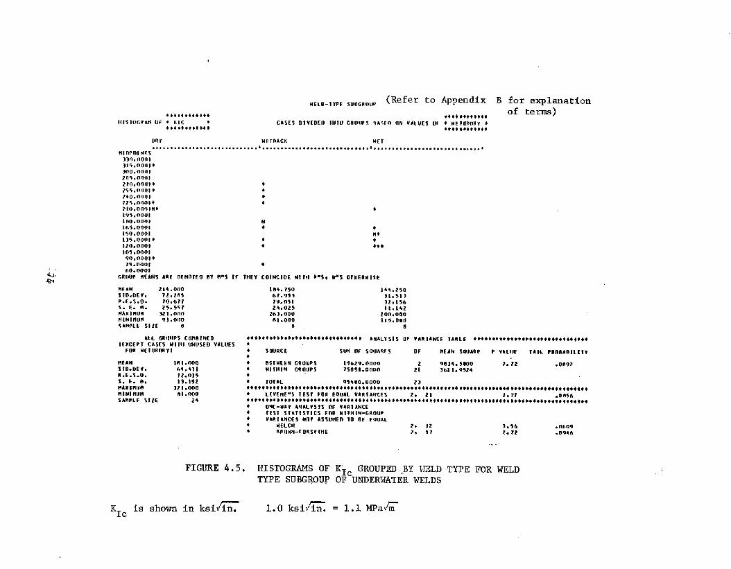
(Refer to Appendix B for explanationwELo-lrPf SUOCROLJP
********+4** ●*4*4*******of terms)
N15!UGRM4 Of * KIC * c~5E5 o]v[fl~~ lt#lLt GMOUP5 MA5E0 flN ViLUEj o} 4 IAE~oRon7 t4*********** ****+*4*****
ORv )IEIRACK HEt. . . . . . . . . . . . . . . . . . . . . . . . . . . . . . . . . . . . . . . . . . ● ...,,*.**.*., ● . . . . . . . . . . . . . . . . . . . . . . . . . . . . . . . . .
nloPol N[s130.000)315. oonl*300.00N1.?05.0001zfo. oou)4 *
?55.00UI* ●
)+0.00IIJ ●
2/5.0001+ 4
Zlo.000)rl*1V5.0001ino. oon# Nlh5.01301 +150.0001135.0001+ *
1?0.000) *
105.000190.13001*75. rloot *flo.000#
GRUUP HEAPAS ARE OEMOrf O E17 PI-S IF THEY CO INCIOE ult!I *-$, MM5 0? IIERU15E
PIFAN .?14.000SIO. F)EV. ?z. zn5R. f. S.O. ?0.67$S. E. M. 25.55?wA!tl MuM 321 .OnoHINIMUH 93.0120$fiMPLF SIZE 8
ALL CROUPS COMBINEDtFECEPt CASES Ullll UNUSEO VfiL.lfES
FOR lAEIORORrl
IIEAM Iml.000STO. OEV. 6!. +31n. E.5.0i ?2.0155. E. m. 13.152MAXIMUM 111.000rllwlmum 01.000SAMPLE S1lE
K~c iS shown
104. 7s0 14~..25o6r.953 31.513?9.051 32.154.?4.025 11.142
263.000 2on.000?li.000 La5.000
n, 8
●*****4++********************* * hNALYsl$ OF V4RtANCE tAn LE +*4+4 *4+++ *+?++ *44*+ *++*44****4*+ SOURCE SUH OF SOUARFS OF MEAN SOUAUE F VILUE IAIL PROt3ARtE_t Tr4* nEr HEEM GROUPS 194z~. nooo 2 ~el+. scoo ?. ?2*
.onw!Al~141N GitlEUP5 75051.00430 .21 3611. q524
*b 10rhL ?5400.0000 23***** ******#****************+ *4*** *********************** ***+* 4***+**+**********+**** ****4bfi● LCVENE*5 lES1 FOa EOL)AL VA R! At7CES 2* ?1 1.77 .On%fl* ************+4**+*********** *+**************+******* **** ***********************************
FIGURE 4*5.
in ksi~
Q~E-MAY AWLr5!5 OF VARIANCETEST 5tATt Sll CS FnR HI! NIP4-GROUFvARl Af4CE5 Hllf hSSUHEi3 VO OE EQUAL
HfLCHFIPOUN-FOKSrrME
HISTOGRAMS OFTYPE SUBGROUP
2, 12 l,5bz, 1?
.0609?. 72 .oqi&
.. . .
K~c GROUPEI.,$Y WELD TYPE FOR WELDOF UNDERWATERWELDS
= 1.1 MPaG
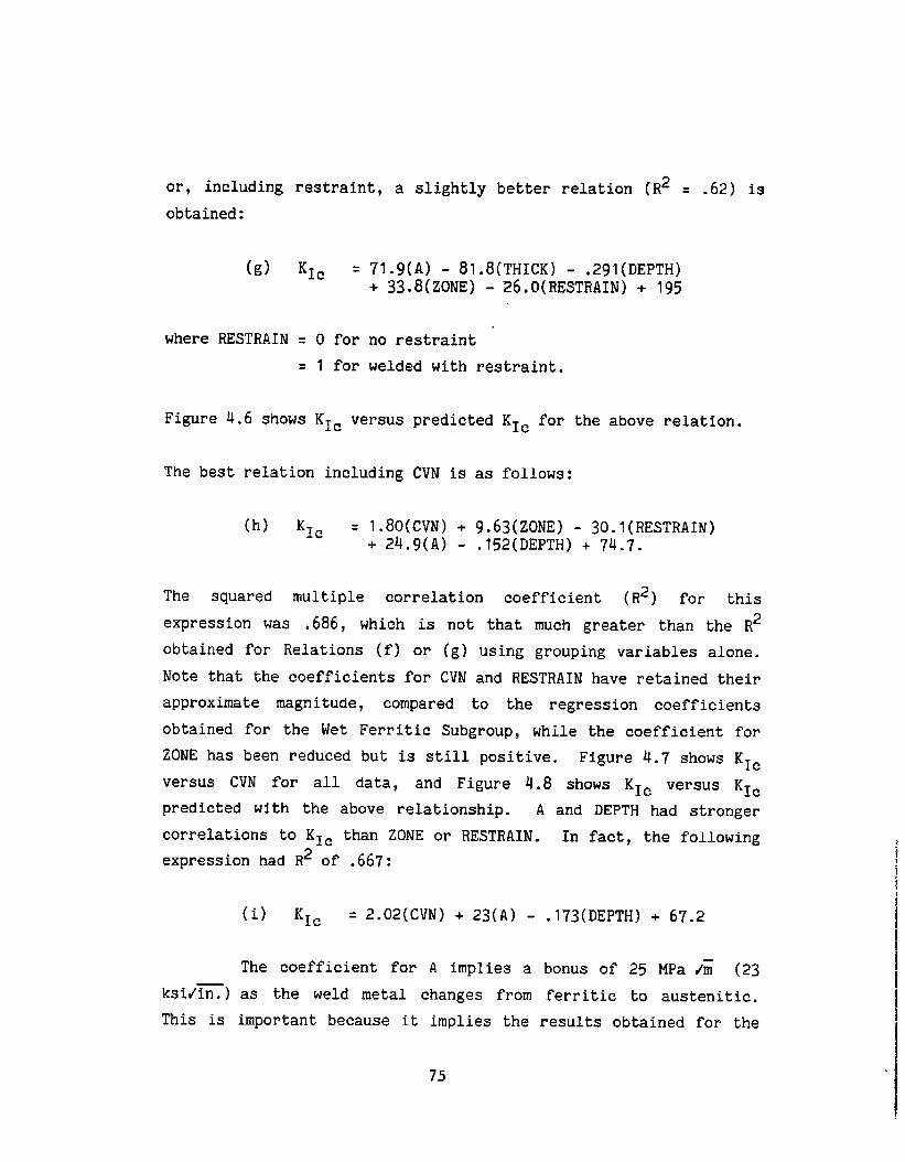
or, including restraint, a slightly better relation (R2 = .62) is
obtained:
where RESTRAIN ❑ O for
= 1 for
71.9(A) -81.8(THICK) - .291(DEpTH)+ 33.8(zoNE) - 26.O(RESTRAIN) + 195
no restraint
welded with restraint.
Figure 4.6 shows KIC versus predicted KIC for the above relation.
The best relation including CVN is as follows:
(h) ‘Ic = 1.80(CVN) + 9.63(ZONE) - 30.I(RESTRAIN)+ 24.9(A) - .152(DEPTH) + 74.7.
The squared multiple correlation coefficient (R2) for this
expression was .686, which is not that much greater than the R2
obtained for Relations (f) or (g) using grouping variables alone.
Note that the coefficients for CVN and RESTRAIN have retained their
approximate magnitude, compared to the regression coefficients
obtained for the Wet Ferritic Subgroup, while the coefficient for
ZONE has been reduced but is still positive. Figure 4.7 shows KIC
versus CVN for all data, and Figure 4.8 shows KIC versus KIC
predicted with the above relationship. A and DEPTH had stronger
correlations to KIC than ZONE or RESTRAIN. In fact, the following
expression had R2 of .667:
(i) ‘Ic = 2.02(CVN) + 23(A) - .173(DEPTH) + 67.2
The coefficient for A implies a bonus of 25 MPa i; (23
ksi/~) as the weld metal changes from ferritic to austenitic.
This is important because it implies the results obtained for the
75

350
300
250
2Q0
r5 o
10C
50.
9.0
●✎☞✎✎☛☛☞✎☛☛✎●✎✎☛☛☞☛✎✎☛☞✎✎✎✎☞✎✎✎✎☞✎✎✎✎☞✎✎✎✎☞✎✎✎✎☞✎✎✎✎✎+
.
.●
✎
☞
..●
☞
●
●
..+.9
●
●
☞
●
✎
☞
● 4.Y●
+
4
4
4
4
4
4
4
4 4
4
44 4
4 4 4
4 844
4
44
4
4
44
4
48
4
4
x
●
●
4.●
+
●
;4.
+
●
●
●
4.+
●
●
●
●
+
9●
.●
☞
●
✎
9
●
+
●
●
●
9+
+.* .*.* x . ...+****+ . .**+*.*.+ . .*.+.*..+ ●..*+.*.*+ . . . . .25* 75. 125 175
50.225
100 150v L52
zoo 25@,xCOQ= .7075 Predicted KIC ks i=
~EA4 5Tm DEV* REGRESSION LINEx
RES. flS.149.05 bom253 X= ●62010 *Y+ 56*245
Y 148-051388.4
7b- 515 Y= l. OCO@*X+ 55E-13 2239-0
FIGURE 4.6. RESULTS OF REGRESSION ANALYSIS: KIC VSPREDICTED BY RELATION (g) AS A FUNCTIONOF MATERIAL, THICKNESS, DEPTH, ZONE, ANDRESTRAINT FOR ALL TEST DATA ON UNDERWATERWELDS
1.0 ksi~ = 1.1 MPa&
76

. +.*.*+.***+.* ..+** *.+*. *m+. . * . + * .*.+.X.*+ . . ..+ . . ..y.350
300
25iI
200
150
10C
50.
O*O
+
●
●
✎
●
☞
.●
●
●
☞
●
●
☞
.●
●
☞
●
●
●
●
☞
.Y●
.+
31
1121 1 1 1
1722
11211 2 lZLlIIL
1111111 1112
11 11121
211 111111 11
121 422 111 1 1 212 1
11231
12 21 1182 11
23 131 111 12211
22112
1
+●
✎
●
9+
●
●
●
●
+
●
.
●
●
+
●
●
●
●
+
.
●
●
●
+
●
●
●
●
+
●
●
●
●
☞
●+X...+..*.+ ✎✎✎✎☞✎✎✎✎☞✎✎✎✎☞☛☛✎✎☞☛☛✎☛☞☛☛✎☛☞✎☛✎✎☞☛✎✎✎☞☛
12.50 37*5O 62*5o 87.50 112*50.000 25-00 50.00 75.00 100*O 125-0
152COR= .7951 CVN (ft-lb)
5EAN ST-DEV. REGRESSION LINE RES. MS.x 41.638 23.620 X= .2+543 *Y+ 5.3009 206.58Y 148.05 76.515 Y= 2.5757*X+ 40.807 21 b8m0
. FIGURE 4.7. DISPLAY OF KIC VS CVN FOR ALL TESTDATA ON UNDERWATERWELDS
1.0 ksi~. = 1.1 MPa/& 1.0 ft-lb = 1.356 J
77.i
I
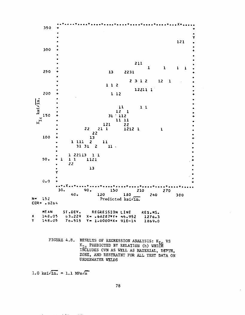
●✎☞✎☛✎✎+m *.* +**.*+...** . *.*+...*+. . ..+....+.. ●x+....*
350
300
250
100
50.
0.0
+
●
●
9
+
●
●
☞
●
●
●
●
☞
9
●
+
●
.●
●
9
+1●
;●
+
2111 1
13 2231
2312 12112
12211 11 12
11 1112 1
31 ‘ 11211 11
121 2222 21 1 1212 1
2213
1 111 2 1131 31 2 11 ~
1 22113 1 111 112122
13
L
+
;121 .
1
1
●
☞
●
●
●
1.+●
●
. .+*X. .+ . . ..+ . ...+....+ . . ..+ . . . .+ . . ..+....+. . ..+.....30. 90. 150 210 270
60. 120 1s0 240 300N= 152 Predicted ksi~COR= .S~64
MEAN ST.DEv. REGRESSION LINE RES.9S.x 14a.05 iJ3.2Z9 X= .68287*Y+ 45.952 1276.3Y 149.05 76.515 Y= I,GOOO*X+ YIE-14 1069.0
FIGURE 4.8. RESULTS OF REGRESSION ANALYSIS: K~c VsKIC PREDICTED BY RELATION (h) WHICHINCLUDES CVN AS WELL AS MATERIAL, DEPTH,ZONE, AND RESTWINT FOR ALL TEST DATA ONUNDERWATERWELDS
1.0 ksi~ = 1.1 MPa&
78

ferritic welds are conservative if applied to austenitic welds as
well. Figure 4.9 shows histograms for KIC grouped by A. (Refer to
Appendix B for definition the terms in Figure 4.9). The mean KIC
for ferritic welds is 158 MPa#= (144 ksi~.) and for austenitic
welds is 238 MPa/~ (217 ksi/F), and the minimum is 89 and
126 MPa#~ (8I and 115 ksi/~ for ferritic and austenitic welds,
respectively.
The residual mean square, i.e., the sum of the squares of
the predicted minus actual KIC for the above relation is 1907 in
English units. For confidence of 95%, the one-sided value of t is
1.65. To bound the regression estimate on the intercept only, we
should subtract 79 MPa/~ (1.65/R=i’2 ksii~) from the regression
relationship. This is doubly conservative, owing to the
conservative estimate of KIC derived from JIC. Further, the weld
can be assumed to be ferritic since the austenitic welds performed
better. The bonus for being in the HAZ can likewise be ignored.
Taking all these factors and the confidence limit into account, the
following simple conservative
(J) ‘IC = 2(CVN)
relationship is offered:
- .15(DEPTH) - 8
where depth for a wet-backed weld is equal to half the acutal
depth.
4.3.2 CVN
Charpy impact energy in itself is useful only as an
indicator of material quality; but because of the
‘It! it is interesting to look at the regression
grouping variables, and compare this to Relations
the previous section.
correlation to
of CVN on the
(f) and (g) in
79

UELO-tYPE SUBGROUP
*******+*+** **+**+*****+MI STOGRAtl OF * I(1C + ChSES OIVIDEO INTO GROUPS IIAsED m $ALUES OF ● A *
************ *4**********
FERRITIC AUStEMll. ***..*.*.. 9*., ****... .*****,.*.. .****4+..6. ●. ..4#4*.. * ● &*b.A**.*. ● *be.*,.*... .+
MII)PnINTs
330.(IOOB315.0001 ●
300.0001285.00082?0.0001 ● *
255.0001* ●
2+0.000) ●
225.0001 m+2L0.000)* **i95.oilolllio.0001lrD5.0001* *150.000)H*135.000)***120.0001** **105.000190.0001*75.000#*ho.000D
~ GRIJUP MEANS ARE tlENOTED BY H*S tF ltlEY COINCIOE ttiTti *-S* t4*S OttihtUISEo
FtFAM 144* 333 zil.66T
ITIJ.OEV. +6,7?5 5~065b11.E.S*O. *%.3hz 58.325S. E. H. 13.503 1?.221Haxl wm 251.000 3zl.oof3MIr41flllH 81.000 115.000SAMPLE S[lF 12 12
hLL GR13UPS COH91ME0 +**+*****+**+********0***++**** AmWYSIS (JF VBRIAMCE TA9LE *0********@40@+*+4@*++*+*s@@oo@4EHCEPT ChSES WITH UNUSEO VALUES ●
FOR CE 1 ● SOURCE SUM OF SQUAWS OF ?WAM SOUARE F VALUE TAfL PRtll)AFItt_tfY*
MFAM L81.000 ● 13ETuEEN GROUPS$TD.OFV.
32266-6+67 1 3226bmt6f)7h4.431
11.23* tiITFfIN GROUPS
. Oozq63213.J333 Zz Z87303333
R.F.s.tl. 72.015 ●
S- E. M. 13.1s2 * TOTAL 95+80-0000 23MAXI HUF 321.000 ******#******+*********t*+**+****************** ****+*********++******** ●**+*+**+*********+**HINtHUfl 81.000 ● LEVENEWS TEST FOR EQUAL VARldNCES I* 22 . w .+51qShHPLE StZE 24 ●*************************** *********+************** ******+***********************+** *******
@ OWE-HAY fiNALYStS OF vAUtANCE● TEST SThTIST~CS FI)R UITM1?I-GRUUP+ VhRtANCES MOT A%SIJMEII TO BE EOUAL# UELCtl 1s 21 11.23#
.0030f!ROtlN-FORSY~WE 1* 21 L1.23 .0030
FIGURE 4.9.‘lsToGws ‘F ‘Ic
GROUPED BY MATERIAL COMBINATION FOR ALL DATA INWELD TYPE SUBGROUP
‘Icshown in ksi~~ ; 1.0 ksi~ = 1.1 MPa&
The following relation is considered optimum and gave an
R2 of .642:
CVN = 26.5(A) + 13.5(zONE) - 25.7(THIcK) - .0804(DEPTH)
+ 51.7
This relation contains the same variables and the coefficients have
the same sign as Relation (f).
4.3.3 Bendscore
Attempts to correlate bendscore with grouping variables
for all data were not very successful. The following relations
were obtained:
(a) BENDSCORE = -.275(DEPTH) - 9.62(A) + 151(R2 = ●S,)
(b) BEND5CORE = -.247(DEPTH) + 76.2(R2 s .29)
Both relationships show the decrease of ductility with increasing
depth, and Relation (a) shows that the ferritic welds were
generally more ductile than austenitic welds.
If the correlation to all-weld-metal tensile test results
were included, excellent relations (valid only for wet ferritic
welds) were obtained:
(c) BENDSCORE = 3.13(AWMPL) - 128.3(R2 = .90)
(d) BENDSCORE = 3.55(AWMSU) - 197.7(R2 = .86)
81

where: AWMPL = all-weld-metal proportional limit in ksi
[1.0 ksi = 6.895 MPa]
AWMSU= all-weld-metal ultimate strength in ksi
[1.0 ksi = 6.895 MPa]
The excellent multiple correlation coefficient (R2) shows how
dependent the Bendscore is on the weld metal tensile properties.
4.3.4 All-Weld-Metal Test Results
The all weld metal tensile test results can be related to
depth, and the following relationships were obtained.
(a) YA PL ❑ 70.4 - .104(DEPTH)(R = .965)
(b) A SU = 81.4 - .088(DEPTH)Y(R = .894)
These relations are valid only for wet ferritic welds. An
attempt was made to relate the percent elongation to depth, but the
elongation was lower for 35 m (115 ft) than for 60 m (198 ft) and
the regression slope was close to zero. The elongation for pairs
of wet ferritic weld metal specimens was:
10 m (33 ft): 12.5 percent, 9.4 percent
35m (115 ft): 6.3 percent, 6.3 percent
60m (198 ft): 9.4 percent, 9.4 percent
Like the hardness data which were lower for 35 m (115 ft) than for
10 or 60 m (33 ft or 198 ft), this may be the result of something
unique in the welding procedure used at 35 m (115 ft). Recall that
the worst fracture toughness 33 MPa/~ (30 ksi/~. also occurred for
the 25.4 mm (1 in.) thick 35 m (115 ft) weld metal.
82

4.4 Summary of Statistical Analysis
The results of laboratory tests (bend tests, Charpy tests,
JIC tests, and all-weld-metal tensile tests) were analyzed with the
statistical analysis computer programs BMDP. The results were
grouped according to carbon equivalent and electrode, weld type,
depth, thickness, weld or HAZ, with or without restraint, and test
temperature, and all combinations of two of these grouping
variables. Analysis of variance was used to determine the
significance of these grouping variables and interactions among the
grouping variables. Regression analysis was used to fit linear
relations between test results and grouping variables and other
test results. In general, the number of tests performed is
sufficient to support the conclusions below with good statistical
significance.
The following relation for KIC, based on weld metal/base
metal thickness, depth, and zone (weld or HAZ) was developed:
KIC ❑ 75.1(A) - 94.2(THICK) - .321(DEPTH) + SS.9(ZONE)+ 201
where: A = O for ferritic welds and A-36 base plate,1 for austenitic welds and A516 base plate
THICK = thickness in inches [1.0 in. = 25.4 mm]
DEPTH = depth of weld preparation in feet[1.0 ft = 0.3048 m]
ZONE ❑ O for weld metal, 1 for HAZ
A slightly better estimate of KIC can be obtained using
the following correlation to the Charpy impact energy, CVN, in ft-
lb:
‘Ic ❑ 2.02(CVN) + 23(A) - .173(DEPTH) + 67.2
83

An expression which contains a 95 percent confidence limit
on the intercept (lower bound) and which provides a conservative
estimate of KIC for all test conditions studied (see Section 4.3.1)
is:
‘I C= 2(CVN) - .15(DEPTH) - 8
It is possible that this conservative expression could
implemented in design guidelines to estimate fracture toughness
underwater welds. If the resultant toughness cannot be shown to
adequate, JIC or CTOD testing could be required.
be
of
be
Other significant findings of the statistical analysis
include:
1) The austenitic welds evaluated have greater KIC than
the ferritic welds, especially for dry and wet-backed welds, and
toughness decreases with increasing depth.
2) The ductility of ferritic wet-backed welds and
austenitic wet welds is very poor.
3) Increased thickness had a small deleterious effect on
toughness and hardness, but had no effect on ductility.
4) HAZ specimens removed from 12.T mm (1/2 in. )-thick
welds were significantly tougher than the corresponding weld metal
specimens. The 25.4 mm (1 in.)-thick specimens had roughly equal
HAZ and weld metal toughness.
5) Temperature changes within the service temperature
range of marine structures had no significant effect on impact
toughness.
6) Restraint had a possible deleterious effect on
toughness, but there is approximately 34 percent probability of
error in this
this chance of
conclusion. However, it is conservative to accept
error and consider the effect of restraint.
84

7) Restraint had no significant effect on ductility or
hardness.
8) Hardness of austenitic welds was significantly
greater than hardness of ferritic welds, and wet welds were much
harder than dry or wet-backed welds. Results from the literature
and service experience reported in Section 2.2.1 of this report
included the following regression relations:
HVN = 157 + 566(CE) for wet-backed welds
HVN = 282 + 566(CE) for wet welds
The relations given above correctly predicted the effect of carbon
equivalent and weld type but overestimated the hardness of wet-
backed welds by about 150, and the hardness of wet welds by about
230, as shown in the following table.
Predicted Observed Mean HVNWeld Type Peak HVN for 33-ft Depth
Wet-backed ferritic 36o 230
Wet-backed austenitic 417 246
Wet ferritic 485 236
Wet austenitic 542 329
Since these relations were formulated to predict peak hardness
(i.e., HAZ near weld crown) while the observed mean is an average
of peak weld-metal-crown hardness and peak midplane HAZ hardness
(i.e., the observed hardness excluded HAZ -near weld crown) the
agreement is considered good.
9) Hardness could not be correlated to either weld metal
tensile strength, toughness, or ductility, and therefore is not
considered useful in predicting these properties of the welds.
85

10) The results of bend tests could not be correlated to
grouping variables (e.g., depth, CE, thickness, weld type), but the
correlation to all-weld-metal tensile properties (proportional
limit, yield stress , or ultimate strength) was excellent.
11) The correlation
depth was excellent; the
of the weld metal tensile properties to
following results were obtained:
(a) Proportional limit:
(b) Ultimate strength:
Section 2.2.2 of this report gave
‘pl = .1o4- 104(DEPTH), ksi*
‘Uts =81.4- .088(DEPTH), ksi*
the following relation for uut~:
(c) uu~~ = 54.2 + 41.9(THICK) - .037(DEPTH), ksi*.
Since our results were based on all-weld-metal tensile tests from
25.4 mm (1 in.) welds, this expression reduces
25.4 mm (1 in.) welds:
(d) uut- = 96.1 - .037(DEPTH), ksi*
This expression predicts higher strength weld
in these test welds as seen by comparing to Expression (b) above.
to the following for
metal than resulted
Transverse-weld tension tests were conducted, but the results
were not statistically analyzed because fracture occurred in the
base plate for almost all specimens , and the ultimate strength and
yield strength of all test specimens fell within a narrow range
near the specified base plate material” strengths, unaffected by
depth, thickness, restraint, or weld type.
*1.O ksi = 6.895 MPa, Depth in feet: 1.0 ft = .souam
86
5.0 DESIGN GUIDELINES FOR UNDERWATERWET AND WET-BACKED WELDS
5.1 Introduction and Overview
Properties and conditions that could influence the
performance of underwater wet and wet-backed welds include the
state of residual stresses in the weld, yield strength, ductility,
ultimate strength, susceptibility to and characteristics of
discontinuities, rate of subcritical crack propagation due to
fatigue and/or stress corrosion cracking, and fracture toughness.
5.1.1 Residual Stresses
The state of residual stresses is difficult to quantify
even for dry welds. Due to lack of information, one must assume
that residual stresses of magnitude equal to the yield strength of
the base plate or weld material (whichever is lower) may exist
locally in underwater wet welds. Higher residual stresses may be
present in fillet welds, depending on the configuration. Under
applied loads, the strain in the welds may reach up to twice the
yield strain of the base plate or weld metal.
5,1.2 Tensile Strength
The weldments tested in this study exhibited excellent
yield strength and ultimate strength. Most (76 percent) of the
transverse weld tensile specimens failed in the base metal, and
even those that failed in the weld (which were only those prepared
at greater than 10 m (33 ft) depth) exhibited strengths greater
than the minimum specified for the base metal. A rule of thumb
widely used in estimating wet weld performance [ ] suggests that
the strength of wet welds is about 80 percent of the strength of
87

corresponding dry welds. The
strength of the wet weld may
and are at least as high.
5.1.3 Ductility
A rule of
only 50 percent of
thumb [5.1]
experimental data suggests that the
exceed the strength of the dry weld
suggests that wet welds may exhibit
the ductility of corresponding dry welds. In the
transverse weld tension tests of this study, the ductility of the
weld metal was generally not a problem because the base metal
yielded, but the specimens that failed in the weld failed suddenly,
and the load-displacement curves exhibited little or no plastic
deformation. Fillet weld tensile tests exhibited much better
ductility, indicating that the ductility for shear failure (the
primary failure made for the fillet weld tensile specimens) is
better than for direct tension.
All-weld-metal tensile tests were conducted using an
extensometer to measure elongation of the weld metal. These tests
showed the elongation of wet welds ranged from 6.3 percent to 12.5
percent which is about 33 to 66 percent of the 19 percent elonga-
tion required by AWS D3.6 Specification for qualification as Type A
welds (those suitable for use as structurally critical welds) and
about 25 to 50 percent of the 23 percent elongation expected for
the base metal.
Bend tests may indicate the ductility of the welds. Side
bend tests for groove welds (AWS D3.6 Specification) are required
to bend to a radius of 19 mm (3/4 in. or 2T) for Type A welds, but
only (57.2 mm (2.25 in. or 6T) for Type B welds. Dry welds, ferri-
tic wet welds at 10 m (33 ft) and austenitic wet-backed welds 10 m
(33 ft) passed the bend test requirements for Type A. Ferritic
wet-backed welds and austenitic wet welds at 10 m (33 ft) and some
88

ferritic wet welds at 60 m (198 ft) did not qualify as Type B.
(Ferritic wet-backed welds were made with an electrode, E6013, not
normally used for wet-backed welds.) It appears that this
requirement of AWS D3.6 Specification should assure that qualified
Type B welds have at least the ductility observed in these test
plates. However, the fact that the austenitic wet welds did not
pass the bend tests is misleading. The austenitic wet welds
exhibit very” good fracture toughness. Most specimens bend to the
required radius only they exhibited cracks at pores which opened up
greater than 3 mm (1/8 in.) The fact that the weld could tolerate
these cracks at such high strains is actually an indication of the
good toughness.
Fillet weld break-over bend tests were also performed.
The requirements for qualification are not as well defined as the
side bend test, and there is essentially no difference in the
requirements for Type A and Type B welds. None of the specimens
bent 90° but rather fractured at 30° - 45°.
Lack of ductility is a serious but not insurmountable
problem for wet welds. The existence of residual stresses probably
requires that the limited ductility available be used for the shake
down (yielding and redistribution) of these residual stresses.
Fortunately, through proper design, underwater wet welded
repairs, attachments, and even original fabrication can be made
such that the reserve ductility exhibited by dry welds is not
required. The principle involves insuring that the structural
member remote from the wet weld can become fully plastic before the
applied stress (excluding residual stress) in the weld metal
exceeds the its yield stress. These design procedures are
discussed in the following Section 5.2.
89

5.1.4 Susceptibility to Cracking and Other Discontinuities
Probably the biggest concern about underwater welds is the
susceptibility to cracking and other discontinuities. The
weldments for this study were produced in the horizontal flat
position in a dive tank without the problems of visibility, access,
and diver discomfort attendant to welding underwater in the
field. The fabricator inspected the weldments visually, with
magnetic particle technique, and with radiography. It must be
considered, however, that the only weldments containing cracks were
ferritic wet-backed welds made with an electrode not normally used
for this purpose. Other discontinuities (within AWS D3.6
Specification requirements) were found and porosity was severe.
The susceptibility to discontinuities will largely depend on the
experience and skill of the welder/diver.
5.1.5 Resistance to Fracture
In some designs, the problem of fracture occurring because
of the presence of cracks may be accommodated by redundancy and
interruption in the weld to prevent cracks from propagating into
adjacent weld lengths. In other situations, welds may be designed
to turn in directions parallel to the direction of applied
stresses. If the wet is to be used for a fracture critical member,
there must still be considerations of fracture control based on a
minimum toughness requirement in the weld qualification procedures
and a maximum stress based on this toughness and a maximum credible
initial crack size. These restrictions should be more severe for
cases where redundancy cannot be accommodated in the design.
Fortunately, the weldments tested in this study exhibited a ductile
failure mode and sufficient toughness to practically enforce such
requirements. Design details to minimize the impact of cracking
and fracture control guidelines are discussed in Sections 5.3 and
5.4, respectively.
90

5.1.6 Resistance to Subcritical Crack Growth
Environmentally enhanced subcritical crack propagation
under static load or stress corrosion cracking is generally not a
problem in mild steels used in offshore and marine construction.
Gooch [5,3] found underwater welds to be resistant to stress
corrosion cracking (SCC) under normal cathodic protection.
However, the effect of sour gas or cathodic overprotection remains
to be investigation.
Subcritical crack propagation from corrosion fatigue must
be considered. Crack propagation rate data reported by Matlock et
al. [~] indicates that for range in stress intensity factor (AK)
less than about 33 MPa/~ (30 ksiifi. ), the crack propagation rate
for wet welds is generally lower than that of dry welds or base
plate material. However, for higher AK, the crack propagation rate
is high and increases at a much greater exponential rate than dry
welds or base plate material. Together with a maximum credible
initial crack size dependent on the design configuration, pa
requirement could be formulated to limit the normally occurring
cyclic stress range such that the stress intensity factor range
remains well below 33 MPa/~ (30 ksi/~.). In this manner the
underwater weld can be assured to be as resistant to fatigue crack
propagation as a dry weld, and normal fatigue design procedures
applicable to offshore structures should be applicable. Limitation
of cyclic stress from fatigue considerations is discussed in
Section 5.5.
5.1.7 Statement of Design Guidelines
In summary, assuming that wet welding has been selected as
the best approach to the problem, the design guidelines proposed
herein consist of a four step procedure as follows:
91

1) Evaluate the design problem (usually a repair or
modification) for the solution which relies most on
compressive or shear stresses in the wet or wet-
backed welds. The following exanples show designs
which help limit tensile stress in the welds. These
designs may be more complicated and expensive than
the designs currently used by underwater welding
contractors. Naturally, if the conditions of the
repair do not warrant more complicated designs, they
would not be required. However, if the use of Type B
underwater welds was questionable and the alternative
would be a much more expensive dry or hyperbaric
repair, then consideration of the following details
may be worthwhile. Further, because of extensive
redundancy of these designs, NDE requirements may
possibly be made less stringent or waived, resulting
in additional savings. For example;
● if the chord is too small to allow for a large
enough doubler, try to utilize full
encirclement split-sleeve doublers when
doublers are subject to out of plane loads to
distribute the load through compressive contact
stresses to the underlying member (as doubler A
in Figure 5.1.)
● try to use scalloped doublers (as is currently
standard procedure) when doublers are subject
to axial load to maximize weld area and make
most weld area act in shear rather than tension
(as doubler B in Figure 5.1.)
92

-.
“WETWELDFULL ENCIRCLEMENT SPLITSLEEVE DOUBLER
/
tEXISTING CHORD FILLET WELD
INTERRUPTED BEFOREINTERSECTION (TYP)
EXISTINGBRACE
\
~lET WELD
Y,‘\\ / SCALLOPED FULL ENCIRCLEMENT SPLIT/: SLEEVE DOUBLER
/’
DOUBLER “B”
/v
FIGURE 5.1 BIUCE REPLACEMENT
93
● try to use an irregular interlocking connection
when groove welds are subject to tension. Note
that if the repair was for a pipeline, a leak
constitutes a failure and therefore the
complicated split sleeve would not be useful.
For pipeline repairs , only control of toughness
to prevent crack initiation would be useful.
● try to provide as much redundancy as possible.
For exsmple, the addition of clip angles to the
seam weld as shown in Figure 5.2.
● try to change direction of weld, use discontin-
uous weld segments, or take other measures
which can limit the extent of crack propagation
or act as a crack arrestor, as shown in Figure
5.3. Be careful not to create stress
concentrations which would be worse than the
uninterrupted weld.
● design the repair to minimize restraint and
hence reduce the risk of hot cracking.
2) Design the wet weld to be below yield stress when the
weakest link remote from the weld is fully yielded
from” the worst case load combination, as shown in
Figure 5.4.
3) Check maximum stress in the weld for fracture based
on the fracture toughness, maximum credible crack
size, and appropriate stress intensity expression.
Alternatively, the CTOD design curve (PD 6493) [5.4]
may be used to estimate the maximum flaw size for a
94

tin.i-d
l-d&
El
o%1
\\
\ \\ {

WJJ*
%s.mwaq
‘%”$ @‘%uu@w)))s’+,,.,‘
Interlocking Groove
(a)
Discontinuous Fillet
(b)
Discontinuous Fillet
Tabs Shop Welded ToAttachment
,Weld Grinding
(c) (d)
Holes Drilled inGroove Weld
Exploded Viewof Bolt andWasher
(f)
FIGURE 5.3 DETAILS TO LIMIT CIUICK SIZE
96
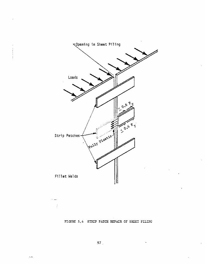
Stri
~Opening in Sheet Piling
-.—
FIGURE 5.4 STRIP PATCH REPAIR OF SHEET PILING
97,

given state of stress. Reduce stress by design
change if necessary.
4) Check maximum frequently occurring alternating
stresses in underwater weld to keep the range in
stress intensity factor well below 33 MPa/= (30
ksi /~.), i.e., in the regime where the crack would
grow faster in the base plate material. Reduce
stress by design change if necessary.
5.2 Design Procedures to Assure Ductility of Wet and Wet-Backed Welded Connections
The design problem that arises from using underwater wet
and wet-backed welds of limited ductility together with members
fabricated from ductile mild steel and dry welds is in some ways
analogous to the problem of using brittle and crack-prone concrete
together with ductile reinforcing steel. The principle involved in
the design of reinforced concrete can be applied to the design of
wet welded connections, i.e., to provide sufficient material to
assure that the weaker material does not reach its limit state
before the ductile material has fully yielded, thus avoiding
undesirable failure and allowing the redundant structure to
redistribute load as the connection yields.
Using such “a limit-state procedure is more rational than
merely using a reduction factor on allowable stress or additional
factor of safety for the weld because it in theory guarantees that
overload failure cannot occur in the wet weld, whereas an allowable
stress approach could still result in wet weld failure. Further,
the limit-state procedure is easier to use because the load used in
the analysis will depend only on the plastic capacity of the
weakest member in the connection, and not on the external loads
98

applied to the structure. The assumed external loads may not be
known, especially when a repair is made to a structure that was
designed many years earlier.
This proposed element of the design procedure can
stated as the following rule:
“The stress in the wet weld should not exceed Fy (where
be
‘Yis the yield stress of base plate or weld metal, whichever is less)
for tensile or compressive stress and 0.6 Fy for shear stress,
under loading which
connection by either
or any combination
highest stress in
perpendicular to the
would fully yield at least one member of the
axial load, bending or torsional moment, shear
loading, whichever combination creates the
the wet weld. Critical cross-sections
applied stress should not be composed entirely
of wet weld (this precludes girth welds) and shall meet the above
requirements .“
The procedure is illustrated in Appendix C in several
examples corresponding to common usage of underwater wet and wet-
backed welding, i.e.,
1)
2)
3)
A full encirclement split sleeve placed over a hole
or crack in a pipeline subject to internal pressure
(e.g., for repair of damaged pipeline).
Strip patches on separating sheet piling subject to
tensile hoop stress (e.g., for littoral sheet-pile
structures retaining soil as shown in Figure 5.4).
Attachment of doublers subject to axial load and
bending (e.g., for replacement of members in offshore
structures as shown in Figure 5.1).
99

5.3 Design Details to Limit Impact of CrackinE
Wet welds (as well as dry welds) are susceptible to
cracking. Even though no welds prepared properly for this program
exhibited cracking, underwater inspection is uncertain and large
initial flaw sizes are possible. However, reasonably small initial
crack sizes can be achieved using stringent procedure control and
quality assurance. If a repair is thought to be so critical that
the designer would have difficulty convincing the owner that Type B
wet welds can be safely used, it may be reasonable to incorporate
in the design some means of limiting the possible initial crack
size or otherwise limit the impact of this cracking on overall
structural integrity. Design details to limit the impact of
cracking on structural integrity will be discussed in the following
categories:
● Details to
● Details to
provide redundancy;
limit crack size in
and
the wet weld.
5.3.1 Details to Provide Redundancy
Any welds are susceptible to cracking and in the ocean
environment these cracks can be expected to propagate and may lead
eventually to instability. Therefore, the designs should
incorporate as much
Sufficient
original structure,
Redundancy
redundancy as is reasonable.
redundancy could possibly be provided by the
if it were highly redundant to begin with.
can be inherent in the design system chosen.
For example, an underwater lift operation could be conducted with
multiple lifting lugs wet welded to the object, and the system
capable of safely completing the lift even if one or more of the
100

lugs were to fail. The design of a repair for a dmaged member of
an offshore structure might entail the addition of two or more new
members to brace the damaged member. The strip patch repair design
of Example 2 in Appendix C is inherently redundant, since a number
of strips could fail without impairing the performance of the
system, and cracks in one strip cannot directly propagate into
other strips.
Redundancy could also be provided by an additional and
completely independent load transfer system. For example, a
cracked plate could be patched inside and out, each patch plate
capable of independently carrying the load in the damaged plate.
Figure 5.2 shows a continuous seam weld required to provide a
watertight seal and capable of carrying the required load. Clip
angles are welded on the opposite side (also capable of carrying
all the load) to provide a backup against complete collapse if the
seam begins to crack.
5.3.2 Details to Limit Crack Size
Because the maximum credible initial crack size in a
continuous wet weld could be too large with respect to the
toughness of the weld and applied stress intensity factor, it may
be necessary to limit the maximum credible crack size by having the
weld change direction (Figure 5.3a and b), using a discontinuous
fillet weld with smooth runout (Figure 5.3c) or using some other
feature to get independent discontinuous welds (tabs like those
shown in Figure 5.3d, holes (with or without the addition of high
strength bolts) like those shown in Figure 5.3e, or grinding as
shown in Figure 5.3f).
Such details should be designed with careful consideration
of the stress concentration that may be caused by the detail.
Y
101

These stress concentrations could create a worse situation than the
continuous weld. Where weld is interrupted but a watertight seal
is required, another material could be used to affect the seal.
5.4 Fracture Control Guidelines
The fracture control requirements should reflect the de-
gree of redundancy and control of maximum crack size incorporated
in the design. The fracture toughness may be determined directly
through JIC testing of the weld qualification test plate, through a
correlation to Charpy impact energy which has been shown to be con-
servative for the materials involved such as the correlation
developed in this study (see Section 4.3.1), or just estimated from
available data on similar weld material. The uncertainty inherent
in these estimates of toughness should also be reflected in the
guidelines. Alternatively, the CTOD design curve (PD 6493) [5.4]
can be used. This empirical design curve is based on much
experience and already contains a sufficient margin of safety.
The method of evaluating the weld for possible fracture
involves a basic fracture mechanics analysis wherein:
1)
2)
3)
A critical location and maximum credible critical
size of a flaw is identified.
The maximum credible nominal stress in the weld is
calculated, or may be conservatively taken as Fy (the
yield strength of weld metal or base plate whichever
is less).
The maximum credible stress iTItenSity faCtOr (~ax)
is calculated with 1) and 2) and established stress
analysis procedures or handbook solutions for K.
102

Factors of safety to account for uncertainty should
be applied to the crack length and stress. Alter-
natively, the procedures of PD 6493 may be employed.
4) The material toughness (KIC or CTOD) is obtained, and
reduction factors applied to the toughness.
5) If KIC < %x, design Changes are implemented and the
process repeated. For the CTOD curve approach,
if ; ~ax (the maximum tolerable flaw size) is less
than the estimate of the maximum critical flaw size,
the design changes are implemented and the process
repeated.
Table 5.1 contains suggested factors of safety for use
with fracture mechanics analysis which are devised in a way which
rationally reflects redundancy, control of crack size, and method
of obtaining KIC.
The above guidelines are implemented and illustrated in
the examples of Appendix C. As a general notion of what size
cracks would be allowed according to the toughness data collected
in this program , consider the following:
● minimum toughness levels for we~ds prepared at 10 m
(33 ft) depth are about 110 MPa/m ( 100 ksiifi. );
● a through thickness crack in a. wide plate would havea stress intensity factor equal to or less than about1.2 u i= (where u = applied stress and a = half thetotal crack length);
103

T!’lBLE 5.1
4 SUGGESTED LOADFACTORSAND STWWGTHREDUCTION FACTOF@
Reduction Factor on Total Efrec ti veControl of Factor on Esthnate or Factor on Degree OF Applied Factor nCrack Size Crack Length iToughness Toughness Redundancy Stress Safety
Changed direction 2.0but stresses remaintensile A
B t.8
No control 4.0 Similar Haterialc
Charpy Test
JIC or CTOD
Similar Materialc
Charpy Test
JIC or CTOD
Sini~lar Materialc
Changed direction 1.6into shear stress A
Charpy Test
JIC or CTOD
Similar Materialc
Charpy Test
JIC or CTOD
0.5
0.67
0.83
0.5
0,67
0.83
0.5
0.67
0,83
0.5
0.67
0.83
D
E
F
D
E
F
:
F
D
E
F
D
E
F
D
E
F
D
E
F
D
E
F
D
E
F
D
E
F
D
E
F
D
E
F
1.8G1.41.2
1.8G1.41.2
, ,8G
1.41.2
, ,8G
1.U1.2
, .BG
1.41.2
~ ,8G
1.41.2
,*8G
1.41.2
, .8G
).41.2
, .8G
1.41.2
,*8G
1.41.2
~,8G
1.41,2
, ,8G
?.41.2
E4.B
?:3.6
4,43.42.8
5.0:.;
3.82.92.5
3.12.42.0
4.83.83.2
3.62.82.4
3.02.31.9
4.63.53.0
2.82,72.3
2.82.21.8

Control ofCrack Size
TABLE 5.1 (Cent’d.)SUGGESTED LOAD FACTORSAND STRENGTH REDUCTION FACTORS
Factor on Estimate ofCrack Length Toughness
B I .0 S!milar t.iaterialc
DiscontinuousWeld A 1.4
Charpy Test
J~~ or CTOD
Similar Materialc
Charpy Test
Jlc or CIOD
B I .0 Similar Haterlalc
Charpy Test
J* ~ or Croll
Redllct.ion
Factor onToughness
0.5
0.67
0.83
0,5
0.67
0.83
0.5
0.67
0.83
Degree ofWdundancy
DEF
DEF
DEF
DEf?
DE
F
D
E
F
D
E
F
D
E
F
D
E
F
Factor onllppliedSkress
,*8G
1,41.2
, @
1.41.2
,*BG
I .41.2
, -Ho
1.41.2
,,~c
1 .fl1.2
, .~G
l.q1,2
, ,,OG
I.u1,2
, ,BG
1.41,2
,*8G
l.rl1.2
A Crack length in analysis is some maximum credible crack length less than the total contlnousslwatght weld length. if %!henmultiplied by the factor, the crack length e~ceeds that whichwould be calculated by D below, that procedure can be used,
B Crack length is the total continuous straight weld length.C Toughness was estimated horn available toughness data for a similar material,D NO redundancy.E ‘rlo I ndepe!!clent and redundant loafl trmmrer systems are used.
F Hultlple (greater than E) redundancy is provided. ~C tlse 1.8 t!mes design tnaxlmum stress or 1.0 times yield stress, whichever is Iese,
H hssurnes that the stress intensl ty factor is proportional to the square root of crack length.
Total EfTect~ve
Factor n
Safety11
3.62.82.4
2.’/2.1t.a
2.2t.71.4
U.33.32.B
3.22.52.1
2.62.01.7
3,62.82,4
2.72,1I.e
2.21.7I.4

● if stresses about 250 MPa (36 ksi) were applied(yield stress for A-36 ) the maximum half crack lengthwould be about 43 mm (1.7 in.), or a crack of 86 mm
(3.4 in.) total length could be tolerated.
5.5 Guidelines For Limiting Cyclic Stress To Control FatiEue
Crack Propagation
Obviously, in order to accurately assess the fatigue life
of an underwater welded repair subject to cyclic or repeated loads,
good crack growth rate data at the appropriate range in stress
intensity factor, load ratio, and environment are needed as well as
an accurate estimate of future loads and existing flaw size. Only
limited crack growth rate data for underwater welds have been
generated to date. However, some useful observations may be made
from the existing data of Matlock et al. [5.2] (see Figure 2.1).
Specifically, these data
intensity factor (AK) of about
growth rates of shallow depth wet
suggest that for range in stress
33 MPa#~ (30 ksiifi. ), the crack
welds
generally less than 2.5x10”4 mm/cycle
for AK less than 33 MPa/~ (30 ksi~~.),
water wet welds were less than those
metal. This suggests that if the range—
from several suppliers was
(10-5in/cycle). Further,
the growth rates in under-
of surface welds or base
in stress intensity factor
were kept below 33 MPaim (30 ksi~in.), a worst-case fatigue
analysis could be performed using data applicable to the base
metal, which is more plentiful. Such fatigue analysis
methodologies using either fracture mechanics or the Miner’s rule
(S-N) approach are well established and will not be reviewed
herein.
The design guidelines for fatigue amount to a limitation
of the range in stress intensity factor and may be stated as
follows:
106

1) Calculate the maximum credible nominal stress range
that may occur more than 10,000 times in the lifetime
of the wet weld. (10,OOO is chosen because less
frequent stress ranges which may cause a range in
stress intensity factor greater than 33 MPa/=
(30MPa ksi~~) will probably still have growth
rates much less than 2.5xIO”3 mm/cycle or (10”4
in./cycle), probably resulting in less than 25.4 mm
(1 in.) of crack growth over the life of the
structure, which seems tolerable for shallow welds
with good fracture toughness. Further, occasional
overloads act to retard crack growth which is
beneficial.)
2) Identify the critical location and the maximum
credible crack size at the beginning of the
lifetime. (This maximum credible initial crack size
could rationally be much less than the maximum
credible critical crack size used in the fracture
control guidelines of the previous section. )
3) Maximum credible frequently occurring A~ax is
calculated from 1) and 2) and established stress
analysis procedures or handbook solutions for K.
4) If b~x >33 MPaJ~ (30 ksii~), design changes are
implemented and the process repeated.
5) If A$ax <33 MPa/~ (30 ksi/F), fatigue life calcu-
lations are performed according to established proce-
dures using base plate material properties (crack
growth rate data or S-N data).
107

6) If fatigue life calculated is not adequate, design
changes are implemented and the process repeated.
Note the crack growth rate data which show a growth in wet welds
lower than the growth rate for surface welds or base metal (Figure
2.1) are limited to shallow depths only, and this behavior may not
be the same for deeper welds. Clearly there is a need for
additional crack growth rate data for wet welds.
5.6 References
5.1 Grubbs, C.E., and Seth, O.W., “Underwater Wet Welding with
Manual Arc Electrodes”, Published in Underwater Welding
for Offshore Installations, The Welding Institute,
Abington Hall, Abington, Cambridge, 1977.
5.2 Matlock, D.K., Edwards, G.R., Olson, D.L., and Ibarra, S.,
“An Evaluation of the Fatigue Behavior in Surface,
Habitat, and Underwater Wet Welds”, Underwater Welding
Soudage Sous L’Eau, Proceedings of the International
Conference held at Trondheim, Norway, 27-28 June 1983
under the auspices of the International Institute of
Welding, Pergamon Press, Oxford, England, p. 303, 1983.
5.3 Gooch, T.G., “Properties of Underwater Welds, Part 1
Procedural Trials and Part 2 Mechanical Properties,” Metal
Construction, March 1983.
5*4 “British Standards Institution, Guidance on Some Methods
for the Derivation of Acceptance Levels for Defects in
Fusion in Welded Joints,” PD64gs, London, 1980.
!
108.i
I

6.0 SUMMARY, CONCLUSIONS, AND RECOMMENDATIONS
6.1 Use of Wet and Wet-Backed Welds
After an extensive review of the literature, collection of
information from contractors and an experimental program; it is
concluded that the wet and wet-backed shielded metal arc welding
(SMAW) process can produce welds suitable for critical structural
applications. However, the limitations of the welds must be
considered in the design. The design process should include a
thorough consideration of fracture and is therefore inherently more
complicated than standard design practice. Material properties may
be required that are more expensive to obtain than the results of
weld qualification tests. Design details may be required that are
more expensive to fabricate than standard weld details. But these
expenses should be offset by the savings relative to alternatives
of wet and wet-backed welding, e.g., hyperbaric chambers, mini-
habitats, or drydocking. Further savings may result from a more
efficient plan for quality assurance based on fracture mechanics
considerations.
Wet and wet-backed welds can rarely achieve the same
quality as dry welds. Wet welds generally have more quality
problems than wet-backed welds. Two unique aspects of wet and wet-
backed welding are responsible (directly or indirectly) for many of
these quality assurance problems: 1) the rapid quench of the weld
and 2) evolved gases including dissociation of water.
Wet welds are cooled 10 to 15 times faster than dry
welds. Depending on oxygen and manganese content, this cooling may
cause martensite and other brittle transformation structures to
form in the grain coarsened region of the HAZ. These hard
microstructure have limited ductility and are susceptible to
109

hydrogen damage. Additional variables such as arc energy, weld
travel speed, water temperature and water currents make prediction
of microstructure difficult.
Evolved gases manifest as porosity which increases with
depth. The most troublesome gas is hydrogen, which is available to
the weld pool, dissolves into the molten metal and diffuses to the
HAZ. The hydrogen may manifest as HAZ cracking as well as
porosity. Control of hydrogen cracking is the main consideration
in choice of electrode.
It is generally accepted (and supported by this program)
that crack-free ferritic wet welds can be made for base metal
carbon equivalent (CE) less than 0.4. The electrode which works
best seems to be the E6013, an electrode which ironically results
in less ductility and lower radiographic quality than low hydrogen
electrodes in dry welds. The E6013 electrode has been successfully
used in all welding positions. The E7018 electrode is commonly
used for wet-backed welds. Base metals with 0.4 < CE < 0.6 can be
welded with austenitic (high-nickel) electrodes. The commercially
used austenitic electrodes are proprietary. Efforts for this
program to make austenitic wet welds on A-516 steel (CE = 0.46)
deeper than 30 m (100 ft) were not successful.
Another quality problem present in the groove welds
prepared for the experimental program was the presence of two
parallel grooves (along fusion lines) up to 2.5 mm (0.1 in.) deep
due to inadequate joint penetration. It is not known how common
this problem is in the general population of wet welds and it has
been stated that this problem can be avoided by good workmanship.
The American Welding Society (AWS) has published rules
(AWS D3.6, “Specification for Underwater Welding”) for qualifying
110

the welder/diver and welding procedure for underwater welding. AWS
D3.6 defines three types of underwater welds according to some
mechanical and examination requirements. In descending order of
quality level are: Type A, intended for structural applications;
Type B, intended for limited structural applications; and Type C,
for applications where structural quality is not critical. A
fourth type, type O, is intended to have qualities equivalent to
those normally specified by
particular type of work
Welding Code - Steel”).
the code or standard applicable to the
(e.g., ANSI/AWS D1.1-82, “Structural
Data reported in the literature generally conclude that
the wet and wet-backed SMAW process can produce the Type B quality
level for most structural steels.
Experiments including weld
D3.6 specification were performed on
with the E6013 electrode (ferritic)
qualification tests per AWS
a 0.36 CE A-36 steel welded
and a 0.46 CE A-516 steel
welded with a proprietary nickel-alloy electrode (austenitic). Dry
welds, wet-backed welds and wet welds at 10, 20, 30, 35, and 60 m
(33, 66, 99, 115, and 198 ft) were tested. The dry welds, ferritic
wet welds at 10 m (33 ft), and austenitic wet-backed welds
qualified as Type A as far as bend and tensile test requirement.
However, since the all-weld metal tensile test was not performed,
these welds cannot be qualified as Type A. Most welds qualified as
Type B except some ferritic welds at 60 m
welds failed to pass the 6T bend test
longer than 3.3 mm (1/8 in.). However,
(198 ft). Austenitic wet
because pores opened up
austenitic wet welds had
very good toughness. Ferritic wet-backed welds also did not pass
as Type B welds. These ferritic wet-backed welds were prepared
with the E6013 electrode; had the E7018 electrode been used, they
may have been acceptable.
111

The fact that some welds did not qualify as Type B
indicates that the AWS specification is sufficiently
discriminatory.
6.2 Effect of Variables on Weld Quality
The main variables identified through statistical analysis
of data from the literature, from contractors, and from the
experimental program are (in descending order of importance):,
● Material Composition
● Depth
● Thickness
● Location of Notch in Weld (Weld or HAZ)
● Restraint
Material composition includes base metal and weld metal. The
carbon equivalent (CE) of the base metal governs the hardenability
of the HAZ (the limits of CE and choice of electrode were discussed
previously). Thust the material composition has a direct effect on
ductility, susceptibility to cracking (RT/VT acceptability), and
toughness. Bend test results were most dramatically affected;
austenitic wet welds exhibited poor bend test ductility attributed
to grain boundary segregates. A-36 base metal produces better
RT/VT acceptability than low alloy steels, but the austenitic welds
were generally tougher than their ferritic counterparts.
Increasing depth usually means poorer RTWT acceptability,
poorer bend test results, and poorer toughness. Possible mechanisms
for this degradation with depth include the increase in porosity
with depth. The orientation of elongated porosity, which is
determined by the welding position, significantly affects the
ability of the weld to pass the bend test. Limited crack growth
, 112

rate data available for underwater welds shows
significant effect on fatigue life and actually
crack ~rowth rate in the high cycle regime.
porosity has a
may retard the
Another mechanism for the degradation of performance with
depth is the changes in weld metal chemistry with depth and
concomitant changes in microstructure. In the ferritic weld metal,
the loss of manganese increases with depth. The loss of manganese
with depth and increasing oxygen content with depth both shift the
CCT diagram to a shorter time for a given cooling rate, resulting
in a lower proportion of fine acicular ferrite. Acicular ferrite
gives a higher resistance to cleavage fracture. Note that the loss
of manganese can possibly be compensated by additional manganese in
the electrodes used for deeper depth.
Thickness has a direct effect on cooling rate (thinner
plates give higher cooling rates), since cooling is thought to be
controlled primarily by conduction through the base metal rather
than heat transfer directly into the water. Thickness has no
apparent effect on ductility. Results from the literature show
that the tensile strength is greater for thicker specimens, but in
this study the welds generally broke in the base metal so this was
not observed. Thicker specimens were observed to have a better
RT/VT acceptability rate.
There is a significant interaction between
the location of the notch for the fracture toughness.
thickness and
Specifically,
the 12.7 mm (1/2 in.) ferritic welds had very tough HAZrelative to
the toughness of the weld. The weld and HAZ toughness of the 25.4
mm (1 in.) ferritic welds were comparable to the lower toughness of
the weld metal. This result is believed to be due to the observed
tendency of the JIC and Charpy fractures to deviate from the 12.7
MM (1/2 in.) HAZ into the base metal, which was not observed for
113

the 25.4 mm (1 in. ) welds. Also the 12.7 mm (1/2 in. ) base metal
may have been tougher than the 25.4 mm (1 in. ) base plate. In
general, however,’ the toughness measured from JIC and Charpy tests
was greater when the notch was located in the HAZ.
Restraint was considered as a possibly important variable.
The effect of restraint is to increase the state of residual stress
and the possibility of cracking. Restrained welds showed poorer
RT/VT acceptability. However, in the experimental program,
restraint could not be shown to significantly effect the various
test results.
Analysis of the literature and contractor data could not
show significance for the effect of polarity, welding position,
water temperature and salinity , and rod or wire diameter.
6.3 Material Property Data and Correlations
Hardness was measured with Vickers 1 kgf test. Maximum
hardness was found in the HAZ in the untempered last passes, 334
HVN1.O for the ferritic wet welds and 46o HVN1.O for the austenitic
wet welds. The hardness was found to be very localized, impressions
0.5 mm (0.02 in.) from the location of maximum hardness were found
to be less hard by as much as 200 HVN. Results in the literature
report hardness above 500 HVN. Wet-backed welds had much lower
hardness than wet welds. The literature and contractor data
suggested the following correlation:
HVN ❑ 157 + 566 (CE) for wet-backed welds
HVN = 282 + 566 (CE) for wet welds
where: CE = carbon equivalent in percent.
114

In the experimental program, hardness could not be successfully
correlated to the depth or thickness. Interestingly, none of the
test results (e.g., bend test, JIC test, Charpy test, or tensile
test) could be correlated to hardness, indicating hardness is not a
factor in weld performance although it may be an indirect indicator
for susceptibility to hydrogen cracking in ferritic welds.
Statistical analysis revealed that RT/VT acceptability
increased with increasing plate thickness, decreasing water depth
and increasing water temperature. RT/VT acceptability for A-36
plates was better than for low-alloy plates.
There was very little toughness, fatigue or Charpy data
available from the literature or from contractors. Results from
this study (applicable only to the two materials tested) suggest
the following correlation of KIC to carbon equivalent, thickness,
depth, and location of the notch (weld or HAZ):
KIe ❑ 75.1(A) - 94.2(THICK) - .321(DEPTH) + 33.9(ZONE) +201
where: ‘Ic = fracture toughness, ksi/~
[1.0 ksi/~ = 1.1 MPa#~]
A = O for A-36/ferritic weld,1 for A-516/austenitic weld
THICK ❑ thickness in inches [1.0 in. = 25.4 mm]
DEPTH = depth of weld preparation in feet
[1.0 ft = 0.s048m]
ZONE = O for weld metal, 1 for HAZ
ranged from 33.163 MPa/~
and from 126 to 179 MPa#=
metal.
(30-148 ksi~fi.) for
(115 to 163 ksiifi.)
115

The correlation for Charpy impact toughness shows the same
trends:
CVN ❑ 26.6(A) - 25.7(THICK) - .0804(DEPTH) + 13.5(ZONE) + 52.1
where: CVN ❑ impact toughness (ft-lbs). [1.0 ft-lb = 1.356 J]
CVN at -2°C (28”F) for wet welds ranged from 20-48 J (15-35 ft-lbs)
for ferritic weld metal, and from 45-117 J (33-86 ft-lbs) for
austenitic weld metal.
The apparent detrimental effect of thickness and benefi-
cial effect of having the notch in the HAZ reflect the previously
discussed observation that the 12.7 mm (1/2 in.) ferritic wet welds
had very tough HAZ, and often the crack deviated into (preferred)
the base metal in these tests.
The HAZ was generally tougher in all types of welds, and
toughness was generally reduced by increasing depth.
A slightly better estimate of KIC can be obtained using
the following correlation to the Charpy impact energy, CVN, in ft-
lb:
‘Ic ❑ 2.02(CVN) + 23(A) - .173(DEPTH) + 67.2
An expression which contains a 95 percent confidence limit
on the intercept (lower bound) and which provides a conservative
estimate of KIC for all test conditions studied (see Section 4.3.1)
is:
‘Ic = 2(CVN) - .15(DEPTH) - 8
116

It is suggested that this relation be used as part of the
design guidelines to estimate toughness from CVN data. The
expression will give very low estimates of the ‘.oughness for CVN
less than 40 J (30 ft-lbs), and if the estimate of toughness is not
adequate, the guidelines suggest that the designer go to the
expense of obtaining an estimate of KIC directly from JIC or CTOD
type tests.
Bend test results are chiefly influenced by material
composition (austenitic wet welds showed poor results) and depth
(increasing depth decreased bend test performance, probably due to
increased porosity with depth). The literature and contractor data
suggested polarity may be significant (DCSP is better). The
correlation to the primary variables was poor, but the bend test
performance was highly correlated to either weld metal tensile
strength or proportional limit, i.e.,
BENDSCORE = 3.13(AWMPL) - 128.3
BENDSCORE = 3.55(AWMSU) - 197.7
where: AWMPL ❑ all-weld-metal
AWMSU ❑ all-weld-metal
Fillet weld break-over
ferritic welds at three depths.
more than 45° before breaking,
Iproportional limit in ksi*
ultimate strength in ksi*
bend tests were performed on wet
None of the specimens bent over
but all met the requirements for
Type B welds.
All-weld-metal
in.) thick wet ferritic
tensile tests were conducted on 25.4 mm (1
welds at three depths. The correlation of
the weld metal tensile properties (in ksi) to depth (in feet) was
*1.O ksi = 6.895 MPa
117

excellent; the following results were obtained:
(a) Proportional limit: Dpl = 70.4 - .104(DEPTH), ksi*
(b) Ultimate strength: uut~ = 81.4 - .088(DEPTH), ksi*
Analysis of the contractor and literature data gave the following
relation for uut~ of welds from transverse weld tension tests:
(d) outs ❑ 54.2 + 41.9( THIcK) - .037 (DEPTH), ksi*
since our results were based on all-weld-metal tensile tests from
25.4 mm (1 in.) welds, this expression reduces to the following for
25.4 mm (1 in.) welds:
(e) uut~ ❑ 96.1 - .037(DEPTH), ksi*
This expression predicts higher strength weld metal than resulted
in these test welds as seen by comparing to Expression (b) above.
Transverse weld tensile test results from this study
showed little variability because 76 percent of these tests
fractured in the base metal, yielding identical results. The
tendency to fracture in
. porosity). The fractures
strength comparable to the
exhibiting little ductility.
the weld increased with depth (and
which occurred in the weld exhibited
base metal but failures were abrupt,
Fillet weld tensile tests
as Type A welds, i.e., the shear
were performed and all qualified
strength exceeded 60 percent of
the all-weld-metal tensile strength and 60 percent of the minimum
specified base metal tensile strength. Shear strength ranged from
*1.O ksi = 6.895 MPa
118

310 to 379 MPa (45 to 55 ksi). The failures were ductile, i.e.
considerable extension (sliding apart) took place prior to
separation.
6.4 Summary of Design Guidelines
Properties and conditions that could influence the
performance of underwater wet and wet-backed welds include the
state of residual stresses in the weld, yield strength, ductility,
ultimate strength, susceptibility to and characteristics of
discontinuities, rate of subcritical crack propagation due to
fatigue and/or stress corrosion cracking, and fracture toughness.
The state of residual stresses is difficult to quantify
even for dry welds. Due to lack of information, one must assume
that residual stresses of magnitude equal to the yield strength of
the weld metal may exist locally in underwater wet or wet-backed
welds. If the direction of the residual stress under consideration
is such that yielding of the base plate would occur prior to
yielding of the weld metal, then the residual stresses should be
assumed of magnitude equal to the base plate yield strength.
The yield strength of the wet and wet-backed weld metals
in this program exceeded base plate yield strength, i.e. the welds
were overmatched. .Note that this overmatching could not be assured
if these weld metals were used with higher strength base
materials.
Reserve ductility of the wet or wet-backed welds
never be counted upon, i.e., the design should incorporate a
link” that fails before
assured by overmatching
ment, techniques which
the weld yields. Note that this
plate
should
“weak-
can be
weld metal and providing weld reinforce-
are commonly used for dry welds. Thus ,
119

incorporating a “weak-link” is just prudent design, and is not
meant to alarm or detract from the usefulness of underwater
welding.
The possibility of cracking, subcritical crack growth, and
fracture should be dealt with explicitly. Again, this is prudent
design procedure and should probably be followed in design of dry
welded connections as well.
Assuming that wet welding has been selected as the best
approach to the problem, the design guidelines proposed herein
consist of a four step procedure as follows:
1)
2)
3)
Evaluate the design problem (usually a repair or
modification) for the solution which relies least on
tensile stresses in the wet or wet-backed welds. Try
to use as much redundancy as is reasonable, minimize
restraint and use details which can limit the size of
initial cracks. Examples are provided in Section
5.3.
Design the wet weld such that applied stress is below
yield stress when the weakest link remote from the
weld is fully yielded from the worst case load
combination.
Check maximum stress in the weld for fracture based
on the fracture toughness, maximum credible crack
size, and appropriate stress intensity expression
taking into account residual stress distribution in
the weld. Alternatively the empirically based CTOD
design curve could be used. Reduce stress by design
change if necessary.
120

4) Check maximum frequently occurring alternating
stresses in underwater weld to keep the range in
stress intensity factor well below 33 MPa/~ (30
ksiiin.), i.e., in the regime where the crack would
grow faster in the base plate material. This assures
that standard fatigue design procedures applicable to
offshore structures will be satisfactory for the
underwater weld. Reduce stress by design change if
necessary.
Safety from overload tensile failure is assured by the
limit state procedure Step 2. This procedure is more rational than
simply specifying a factor of safety on tensile strength.
For the fracture assessment (Step 3) a system of safety
factors is developed in Section 5.4. The system includes a factor
on crack length (ranging from 1.0 to 4.0) based on how this crack
length was estimated and design details (if any) to limit crack
size. There is a reduction factor on toughness (ranging from 0.83
to 0.5) based on how the toughness was estimated (e.g., a JTC test
could be performed (0.83), or the toughness could be assumed to be
equal to the toughness of a similar material welded under similar
conditions (0.5)). Finally, there is a factor on applied nominal
stress (ranging from 1.2 to 1.8) based on the degree of redundancy.
(The CTOD design curve has a sufficient margin of safety built into
it and such factors are not applicable for the CTOD approach.)
The total effect of these factors when implemented in a
fracture mechanics assessment can be equated to a total factor of
safety. For example, consider the largest and smallest possible
safety factors:
121

● Total factor of safety of 7.2 - no control of initial
crack size, toughness estimated from a similar
material, and no redundancy.
● Total factor of safety of 1.4 - crack control is
provided by using discontinuous lengths of weld,
toughness is estimated by performing a JIC test, and
multiple redundancy is provided by the design.
Fatigue life calculations should be performed using
realistic (unfactored) stresses, crack growth rate data, and crack
lengths. The reduction in toughness described above should be
used; this will provide a sufficient margin of safety on life.
6.5 Conclusions
1. The data gathered from industry sources and from the
literature, and the experimental data obtained
provide a basis for the use of the wet and wet-backed
SMAW process for critical structural applications
provided the limitations of the welds are considered
in the design.
2. Despite severe porosity which significantly reduces
the net area, the tensile strength of the welds
exceeds the rated strength of the ferritic electrode
414 MPa (6o ksi) and exceeds 552 MPa (8o ksi) for the
austenitic welds. The shear strength of fillet welds
exceeds both 60 percent of the base metal minimum
tensile strength and 60 percent of the all-weld-metal
tensile strength.
122

3. Ductility of these welds is limited. Maximum bend
test radius for the deeper ferritic welds is 6T or
57.2 mm (2.25 in.). The austenitic wet welds could
not bend to this radius without opening up pores
greater than 3.3 mm (1/8 in.) and therefore did not
qualify as Type B welds. Because these austenitic
welds are very tough and strong and otherwise appear
to be suitable for use as structurally critical
welds, perhaps this requirement of AWS D3.6
Specification should be reconsidered for austenitic
welds. The elongation for the ferritic all-weld-
metal tests ranged from 6.3 percent to 12.5 percent.
4. The fracture toughness of the welds is sufficient to
tolerate flaws (without initiating tearing) larger
than those allowed under .AWS D3.6 Specification
3.3 mm (1/8 in.) in the presence of stresses as high
as the minimum strength of the weld metal 414 MPa
(6o ksi). Wet-backed welds and wet welds made at 10m
(33 ft) have fracture toughness (KIC, derived from
JIC) gr@ater than 102 MPa/~ (93 ksi~~) Initiation
values of CTOD were greater than 0.09 mm (0.0034
in.). Simple fracture mechanics analysis yield a
tolerable defect size of about 25.4 mm (1 in.) in the
presence of stress as high as the strength of the
weld metal, or about 6.4 mm (1/4 in.) in the presence
of twice the minimum yield stress. The CTOD design
curve procedure requires consideration of residual
stress. The stress considered in a fracture
assessment by the CTOD approach can be as high as
twice the yield stress, and more conservative results
are obtained. For CTOD of 0.09 mm (0.0034 in.), a
tolerable defect size just greater than 3.3 mm (1/8
in.) is obtained.
123
5. The HAZ
(1 in. )
12.7 mm
tougher
is as tough as the weld metal for 25.4 mm
welds and tougher than the weld metal for
(1/2 in. ) welds. Austenitic welds were much
than ferritic welds. Toughness decreases
significantly with depth, probably due to chemical
and microstructural changes as well as increasing
porosity.
6. All fracture toughness tests failed in a ductile
tearing mode. Four of 19 JIc/CTOD tests with the
crack in the HAZ exhibited a pop-in after some stable
tearing. (None of the 29 tests of weld metal popped
in. ) The four plates were all 25.4 mm (1 in.) thick
including a Q ferritic weld 102 MPa/~ (K1C=93
ksi~~), a wet-backed austenitic weld 256 MPa/~
(K1C=233 ksi/~), and a wet austenitic weld
135 MPa/~ (KIC=123 ksii~). All of the pop-ins
arrested and stable tearing was resumed as the
failure mode. The maximum crack jump was about 5.1
mm (0.2 in.).
7. The austenitic weld
ited fully-shear,
and HAZ Charpy specimens exhib-
upper-shelf fracture at -2°C
(28oF). The wet ferritic weld metal was also upper-
shelf at -2°C (28°F). Dry and wet-backed ferritic
welds and the HAZ of the wet ferritic welds were
tougher than the wet ferritic weld metal but were
generally not upper-shelf.
8. No cracks were observed either in NDE or in cutting
up specimens
which were
electrode.
except the ferritic wet-backed welds
intentionally made with an improper
124
>
.1

9. Porosity was excessive in the wet welds and increased
with depth. Slag inclusions and lack of penetration
were found. These discontinuities were acceptable
within AWS D3.6 Specification.
10. Peak hardness in the last passes of the welds,
particularly in the HAZ, was high. Ferritic welds
exceeded 300 HV1.O and austenitic welds exceeded 400
HV1.O. Since 1) no cracking was observed in the
welds, 2) no brittle behavior was exhibited, and 3)
hardness could not be correlated to bend test,
toughness, or strength performance; it is concluded
that the hardness is not a meaningful indicator of
weld quality or performance.
11. Bend test performance correlates well with all-weld-
metal yield and ultimate stress.
12. All-weld-metal yield and ultimate stress correlate
very well (decreasing) with depth.
13. CTOD was shown experimentally to be linearly
proportional to J. Since J and K are analytically
related, all these toughness parameters are
related. KIC (from JIC) was correlated to CVN.
14. Design guidelines were formulated which focus on
design to add redundancy, limit crack size, minimize
restraint, and reduce stress in the weld. The design
guidelines give a procedure for fracture analysis.
An alternative procedure using the British CTOD
design curve would also be applicable. Guidance on
fatigue is also offered, but this is based on limited
data. Example problems illustrate the applicability
and workability of these design procedures.
125

6.6 Recommendations
1.
2.
3.
4.
Underwater wet and wet-backed welding should be
allowed on mar ine structures where presently
prohibited by companies or regulatory agencies.
Underwater welding should be used carefully and
limitations of the welds should be considered in the
design.
More experimental data should be obtained on the
fatigue crack growth rate, SCC susceptibility, and
fracture toughness of these welds. There is
presently enough material left over from the
experiments to extract two compact specimens from
each plate in the test matrix. In view of the
expense of producing these plates, good use could be
made of these specimens for the needed
relatively small cost.
Testing should also be conducted on welds
tests at a
prepared in
poor visibility and in other than the flat horizontal
position.
Transverse weld tension testing could be eliminated
from the AWS D3.6 Specification requirements for
procedure qualification provided adequate bend test
performance has been demonstrated. All-weld-metal
tension tests are useful and should be considered in
requirement for Type B welds. Hardness does not seem
to indicate weld quality or performance, and maximum
hardness requirements could possibly be raised. The
allowable size of opened-up pores in the bend test
could be increased for austenitic welds. Shear
strength requirements of 60 percent of all weld metal
strength can easily be obtained for Type B welds.
126

5. More research should be done on the chemical and
concomitant microstructural changes that occur with
depth. Weld chemistries and microstructure could be
obtained on the scraps of underwater welds from this
project. Porosity should also be quantified for the
welds used in this project.
6. Research should be performed to document and
demonstrate by example the design of underwater
welded repairs in handbook form. The repairs should
be analyzed by finite element methods to obtain hot
spot stresses.
7. There is still a need for continued electrode
development, particularly for an electrode to weld
higher CE materials at depths greater than 10 m (33
ft).
8. Design guidelines, using those proposed herein as a
starting point, should be examined and debated by a
committee and eventually published in the form of
recommended practice.
127
i

APPENDIX A
A.1 Documentation of Welding Parameters
Underwater electrodes were transported to the working
depth using Sea-Con’s patented “Electrode Transfer Device” which
was pressurized to the approximate ambient pressure at the working
depth. Waterproofing of the electrodes is very important but the
techniques and coating are proprietary.
All plate surfaces and edges that were joined by welding
were either sandblasted or ground to clean, sound base metal,
removing all mill scale or rust that was present.
Plates were welded with the stringer bead technique using
Sea-Con’s proprietary electrodes. The E6013 electrode used has
also been modified by Sea-Con.
Table A.1 shows relevant welding parameters including the
initials of the diver, the amperage and voltage range, weld travel
speed, and number of passes. This welding data was incomplete for
the welds 266, 299, 21S and 21D.
A.2 Visual and Radio~raphic Examination
All welds were visually inspected upon receipt at SWRI for
the following defects:
● cracks
● surface porosity
● entrapped slag
● incomplete fusion (both at crown andat root after removal of backing bar)
128

Table A,l
Plate Welder Amp volts Travel PassesSpeed
(in/rein)*
1o-1
10-2
10-311-111-211-3llF-111F-2llF-lT1 lF-2TllB-11 lB-21 lB-312-112-212-312F-112F-212F-lT12F-2T13-113-213-313F-1lSF-213F-lT13F-2T20-120-220-s21T-121T-221-121-221-3-21R-121 R-221 R-321B-121 B-221B-321s-121s-2
GLHGLHGLHGLHCAKCAKGLHGLHGLHGLHCAKCAKCAKCAKCAKCAKCAKCAKCAKCAKCAKCAKCAKCAKCAKCAKCAKGLHGLHGLHCAKCAKCAKCAKCAKCAKCAKCAKCAKCAKCAK(5/32 in.)(5/32 in.)
*1.O in. = 25.4mm
150150150175170170150150150150170 - 165170 - 165175180 - 150150170170170175 - 170175165165165 - 16o16516516516516016o16o17017017017060 - ‘--70707075
::
1“(u
129
2626262628282828282825::
24 “ 182228242424 - 28222828 “ 3024 - 30262828282525252828282826 - 28282828282830
w6-87*7
;!’15.665.65.810.610 611.1 - 6.6
H - 7.99.1 - 128.8107611 - 1210 - 1212 - 13.3
:.53.5;.8
6“86-81010
N8.7
;:;10
9-121011.2 - 13.3
212120222020
:44202624252527336634273333
z.40414345496256835759
&4459

Table Ll(Continued)
Plate Welder Lmlp volts Travel PassesSpeed
(in/rein)*
21D-121D-2266-1266-2299-1299-222-122-222-322R- 122R-222R-322T-222T-223-123-223-323R- I23R-223R-323T-123T-240-140-340-541-141-241-341B-141B-241B-330-230-430-6.31-131-231-331B-131B-231B-3
CAKCAKCAKCAKCAKCAKCAKCAKCAKCAKCAKCAKCAKCAKCAKCAKCAKCAKCAKCAKCAKCAKCAKCAKCAKCAKCAKCAKCAKCAKCAKCAKCAKCAK
170 “ 14085 - 16o6580 - 15065 - 15065 - 1554060
165165170 “ 155165 - 155165165 - 155165 - 150165 “ 160165165165160155 - 150155-15014016o155165165165155155155140 - 155140 - 55155
25 - 2630- 2426 - 2828 - 3024 - 3026 - 302220262624 “ 3024 “ 302426 - 2826 “ 2826 - 28242424
;; - 3230- 31;:
3024242432303030;;
9.1 - 127 - 1210 - 13.3
- 12:?3 - 13*39.1 - 14*110 - 1110.9121212121212 - 1112 - 11
i:; : :5.8 - 6.4;.4 - 7.9
10
;“! 6.36.1 - 8.85- 13.36.4 - 6.75 - 5.65 - 5.613.38-1111 - 12.55 - 8.18.5 “ 10.96.3 - 6
ig
a56666265427377
::799150592830
::3342232624131115131414a
108
1.0 in. = 25.4mm
130
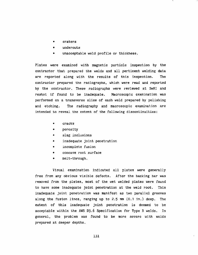
● craters
● undercuts
● unacceptable weld profile or thickness.
Plates were examined with magnetic particle inspection by the
contractor that prepared the welds and all pertinent welding data
are reported along with the results of this inspection. The
contractor prepared the radiographs, which were read and reported
by the contractor. These radiographs were reviewed at SWRI and
reshot if found to be inadequate. Macroscopic examination was
performed on a transverse slice of each weld prepared by polishing
and etching. The radiography and macroscopic examination are
intended to reveal the extent of the following discontinuities:
● cracks
● porosity
● slag inclusions
● inadequate joint penetration
● incomplete fusion
● concave root surface
● melt-through.
Visual examination indicated all plates were generally
free from any obvious visible defects. After the backing bar was
removed from the plates, most of the wet welded plates were found
to have some inadequate joint penetration at the weld root. This
inadequate joint penetration was manifest as two parallel grooves
along the fusion lines, ranging up to 2.5 mm (0.1 in.) deep. The
extent of this inadequate joint penetration is deemed to be
acceptable within the AWS D3.6 Specification for Type B welds. In
general, the problem was found to be more severe with welds
prepared at deeper depths.
131

Specimens were generally suitable for testing. Holes,
arc-strikes, and surface gouges in the base plate were found, but
could be avoided by proper layout of the test specimens. The
majority of the plates were winged or misaligned, a condition which
results from cooling in the absence of restraint.
Magnetic particle examination reports indicated no
detectable defects other than external defects such as poor bead
profile, bead overlap, undercut, low weld-metal, surface porosity,
and indentations. All of the above were deemed acceptable
according to AWS D3.6 Specification for Type A welds.
Radiography and macroscopic examination revealed a variety
of discontinuities. Porosity was, of course, prevalent in the
underwater welds. In most cases, the extent of this porosity was
deemed acceptable within the AWS D3.6 Specification for Type B
welds. The density and size of the pores was found to be related
to the depth of the weld. As an illustration of this phenomenon,
three photographs of 25.4 mm (1 in.) groove weld macroscopic
examination specimens prepared at different depths are presented in
Figure A-1. Unacceptable slag inclusions were found in a few
plates, but in most cases they were avoided during specimen
layout. The inadequate joint penetration at the weld root was also
detectable with radiography (RT).
Recall that three groove weld test plates are available
for each material/depth combination in the test matrix. One plate
was used to extract compact tension specimens for JIC tests,
another plate used for Charpy impact test specimens, and a third
for the macroscopic examination specimen, the transverse weld
tension specimens, and the side bend test specimens. Plates which
contained defects were generally used for the tensile and bend test
specimens.
132
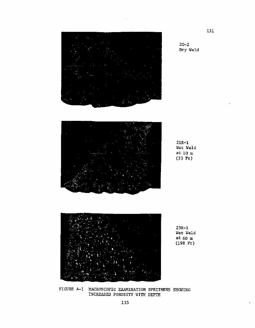
131
20-2Dry Weld
21R-1Wet Weldat 10 .m
(33 Ft)
23 R-1Wet Weldat 60 m
(198 Ft)
FIGLTRX A-1 MACROSCOPIC EXAMINATION SPECIMENS SHOWINGINCREASED POROSITY WITH DEPTH
133

A.3 Side Bend Tests
Figure A-2 shows the test plate layout and the location of
the side bend test specimens. (Also shown is the location of the
“macro” or macroscopic examination and hardness test specimen and
the tensile specimens.) Note that 25.4 mm (1 in.) of material at
the extremities of the plate are discarded.
The side bend test specimen is shown in Figure A-3.
Figure A-4 shows the usual logic of the testing procedure. Recall
that eight bend test specimens are prepared, but only seven tests
are required to be performed. Usually, however, all eight
specimens are tested. Four bend tests at S7.2 mm (2.25 in.) radius
(6T) are performed on all plates. If none of these fail, remaining
specimens are tested at smaller radii as shown in Figure A-4. AWS
D3.6 Specification requires four 6T bend tests be performed for
qualification as Type B welds. All four of these tests pass (i.e.,
not fracture or reveal any defects larger than allowed in the
specification). Therefore, classification of the welds as Type B
depends only on the first four tests. Often, one of the first four
6T bends failed, but further testing showed we could get four or
more bends at 6T to eventually pass. These welds are still not
classified as Type B.
Table A-2 presents the results obtained (pass or fail) on
individual bend specimens. In addition, each weld has been rated
as Type A, B, or C, (only insofar as the results of the bend test)
and a relative score assigned to each plate according to the
following system:
● Since the strain in the bend test is proportional to
the radius of curvature, successful completion of a
bend test is assigned a number of points inversely
134

.,- ..--” ,
—
!
I
& ——— .— ——
“L SI’ua 5t%JP—— —. — ——
I +IPE 6ENP——— ——— —.
I-—————— ——,
+——————” .
---+
II
1
FIGURE A–2 LAYOUT OF TEST PLATE FOR
.
.,
QUALIFICATION TESTS
-.,”..— ....—..—....— .——-—
-,. 13L

I . I !
. .
F-- —t
- =..~i.--4-
%.
FIGURE A-3 SIDE BEND TEST SPECIMEN
136
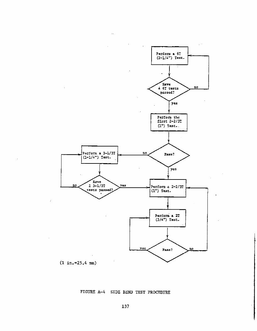
“F=+
+
Petiam theftisz 2-213T(l”)TI=%.
(1-1/4”) Test.
na
zests passed? (l”) Test.
(1 in. =25.4 mm)
FIGURE A-4 SIDE BEND TEST PROCEDURE
137

TABLE A-2BEND TEST RESULTS
Air WeldsA36 A516
Weld Qualification: Type A ASpecimen 10-3 20-: 30-2 40.;
BendRadius Score 100 94 100 94
6T P P P’ P
6T P P P P
6T P P P P
6T P P P P
2 2/3T P P P P
2 2/3T P P
2T P P P P
2T P P P P
2T P P P P
Notes:
P = PassF = FailA Qualifies as Type A as far as the bend test is concerned.B Qualifies as Type B as far as the bend test is concerned.c Does not qualify as a structural weld.
.
138

TABLE A-2 (Cent’ d.)BEND TEST RESULTS
Wet-Backed Welds (33’) (10 m)A36 A516
Weld Qualification: Type c BSpecimen 1 lB-2 21 B-3 31 B-: 41B~3
BendRadius Score 8 63 88 88
6T F*+ F+ P P
6T F*+ P P P
6T 1?+ P P P
6T
6T
P P P P
P P
6T P
6T P
P P
P
F
P
P
P
F
P
2 2/3T
2 2/3T
2T P
2T
Notes:
P = PassF= Fail+ Large visible crack”in machined specimen* In location of known defectA Qualifies as Type A as far as the bend test is concerned.B Qualifies as Type B as far as the bend test is concerned.c Does not qualify as a structural weld.
139

TABLE A-2 (Cent’ d.)BEND TEST RESULTS
Wet Welds (33’) (10 m)A36 A516
Weld Qualification: TypeSpecimen 1!-2 2!-1 21:-1 21:-1 21:-1 3;-3 4:-3BendRadius
6T
6T
6T
6T
6T
6T
6T
6T
2 2/3T
2 2/3T
2T
2T
Score 94 88 20* 80+ 71 23
PP P P PF
PP P P PF
PP F P PP
PP F P PP
P
P
P
P
PP F
PP P
PF F
PP P P
a
F
F
F
P
P
P
P
F
Notes:
= Pass: = Fail* These scores were estimated since only four tests were conducted.A Qualifies aq Type A as far as the bend test is concerned.B Qualifies as Type B as far as the bend test is concerned.c Does not qualify as a structural weld.
140
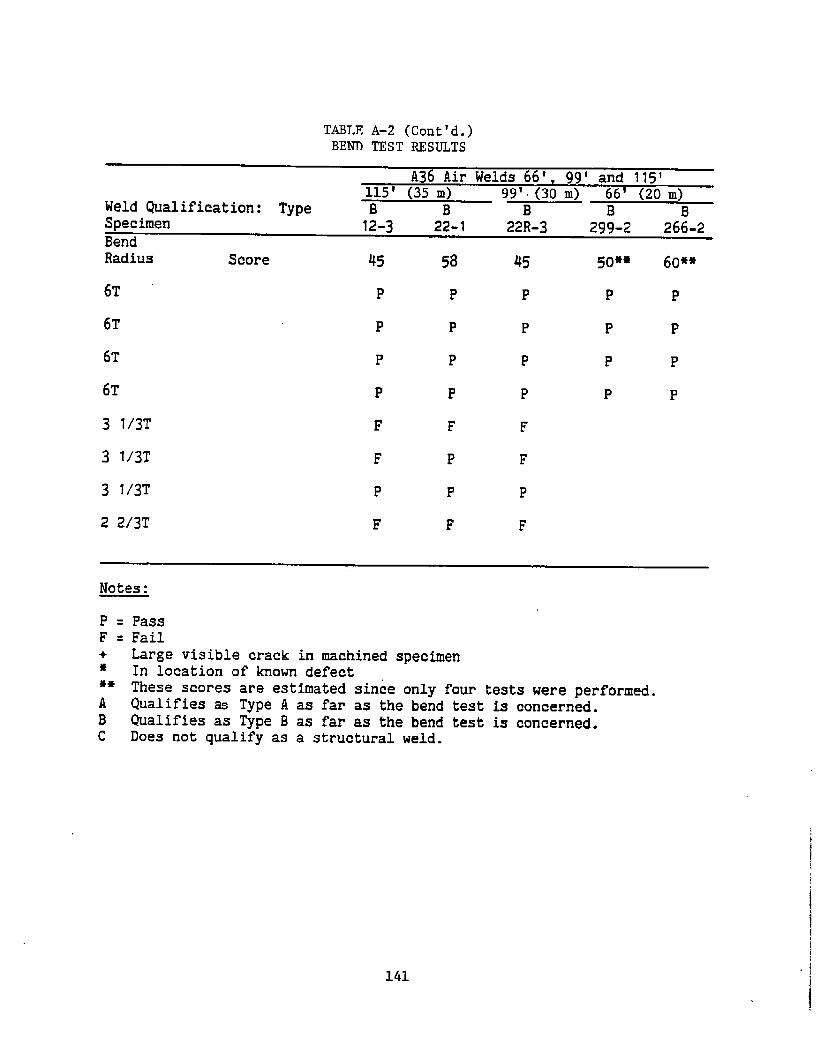
TABLE A-2 (Cent’d.)BEND TEST RESULTS
A36 Air Welds 66’, 99’ and 115’115’ (35 m) 99’ (3O m) 66’ (20m)
Weld Qualification: Type B B B B BSpecimen 12-3 22-1 22R-3 299-2 266-2BendRadius 3core 45 5a 45 50** Go**
6T P P P P P
6T P P P P P
6T P P P P P
6T P P P P P
3 l/3T F F F
3 l/3T F P F
3 l/3T P P P
2 2/3T F F F
Notes :
P = PassF = Fail+ Large visible crack in machined specimen* In location of known defect** These scores are estimated since only four tests were performed.A Qualifies as Type A as far as the bend test is concerned.B Qualifies as Type B as far as the bend test is concerned.c Does not qualify as a structural weld.
141
i

TABLE A-2 (Cent’d.)BEND TEST RESULTS
Wet Welds (198’) (60 m)A36
Weld Qualification: Type B cSpecimen 13-1 2& 23 R-1BendRadius
6T
6T
6T
6T
6T
6T
6T
3 l/3T
3 l/3T
3 l/3T
2 2/3T
Score 31
P
P
P
P
F
F
F
F
23
F
P
P
P
P
38
F
P
P
P
P
P
P
F F
F
F
2 2/3T
2T
2T
2T
Notes:
P = PassF = Fail+ Large visible crack in machined specimen* In location of known defectA Qualifies as Type A as far as the bend test is concerned.B tialifies as Type B as far as the bend test is concerned.c Does not qualify as a structural weld.
142

proportional to the radius, i.e., 1 point for
completion of the 6T bend test, 1.8 points for the
3-1/3T, 2.25 points for the 2-2/3T, and 3 points for
the 2T test.
● One point is subtracted for each 6T bend test that
fails, since this test is essential for
qualification.
● No points are subtracted for failed bend tests at
smaller radii.
● The scoring is done on the basis of seven tests,
including first all 6T bend tests (all failures plus
those that passed, up to seven total). The remainder
of the seven tests, if any, are chosen for maximum
point value.
● The scores are then normalized by dividing by the
highest score (13 points for 10-3 and 30-2) and the
percentage is reported in Table A-2.
All the bend tests from the dry welded plates passed,
qualifying all the welds as Type A as far as the bend test. It was
observed that a very small 0.8 mm (1/32 in.) crack developed in the
12.7 mm (1/2 in.) A-36 plate, and that larger cracks 2.3 mm (3/32
in.) developed in both the A-516 plates. There was no dimpling on
the bent surfaces from porosity observed in these specimens, nor
was there any evidence of inadequate joint penetration at the root
of the welds.
In the wet welds, the extent of inadequate joint
penetration on both sides of the root is significant, and often
143

cracks would form near these discontinuities. Also , there are
visible pores in the weld before bending which would open up or
dimple on either face (compression or tension).
The ferritic wet-backed welds llB-2 and 21B-3 both
contained cracks which were clearly visible upon sawing the
specimen blanks from the plate. Recall that these welds were
prepared with the E6013 electrode, when the E7018 electrode is the
electrode of choice for wet-backed welds. (The E6013 electrode was
used for the dry and wet-backed welds as well as the wet welds to
provide consistency in the test matrix.) The crack surfaces
contained black and aquamarine (light blue) deposits, indicating
the cracks probably occurred while the ,weld was still hot. These
cracks were nearly through the thickness, longitudinal, and
parallel to the vertical edge of the welds. As for 21B-3, this
crack was isolated to one test specimen, but it eluded the
radiographers. Radiographic indications were found for plate llB-2
and it was called out to be about 38.1 mm (1.5 in.) long. However,
this crack was found to extend through one-half of the plate. This
plate (lIB-2) failed to qualify as a structural weld. (The
specimens selected for JIC testing from a companion plate, llB-3,
developed cracks along the fusion line when we tested it, the other
‘Ic specimen from llB-3 had a large through thickness crack that
prevented precracking.) The performance of all bend test specimens
of 21B-3 was good except the cracked specimen which was not tested,
and we allowed this plate to qualify as a Type B weld.
All specimens from plate 21-1 passed with the exception of
one of the 2T bends which fractured. A large 6.4 mm (1/4 in. dia.)
slag deposit was observed at the root of this weld. After testing,
upon review of the RT, it was noted that this slag was called out
in the RT report by both SWRI and the contractor. It is still felt
that this weld should qualify as Type A as far as the bend test.
144 I

In the restrained plate 21 R-1 all the 6T bends passed.
One of the 2-2/3T bends passed, but another developed a 3.3 mm (1/8
in.) crack which was associated with a void in the weld, and is
therefore cause for rejection according to AWS D3.6
Specification. Slag was noted in the SWRI RT report in the
location of this bend specimen, but was not reported by the
contractor. One of the 2T bends passed, although the pores dimpled
and some developed rracks up to 2.3 mm (3/32 in.) long. Another of
the 2T bends fractured. There was no noticeable defect in this
weld except for excessive porosity, and no defects were noted in
either of the RT reports in this location. This plate would only
qualify as a Type B weld as far as the bend test is concerned.
The austenitic wet welds prepared at 10 m (33 ft) yielded
two failed 6T bends in the process of obtaining four 6T bends which
passed. Strict interpretation of the AWS D3.6 Specification (on
page 26, column 1, item (4) in section 4.5.2) would reject these
plates as Type B welds. The austenitic wet-backed welds performed
well, and both qualified as Type A welds.
all
the
Ferritic welds at 20, 30, and 35 m (66, 99, and 115 ft)
qualified as Type B welds, although 6T was about the limit of
consistently passing bend tests.
The ferritic welds at 60 m (198 ft) suffered generally
from extreme porosity. The 6T bends all passed in plate 13-1, but
cracks up to 2.3 mm (3/32 in.) long developed about the pores. One
bend test was attempted at 2-2/3T or 25.4 mm (1 in. radius), but
this specimen fractured. Three tests were then performed at 3-1/3T
or 31.8 mm (1.25 in. radius). One of these fractured, and two
developed cracks greater than 3.3 mm (1/8 in.) long associated with
pores, therefore, all tests at less than 6T failed according to AWS
D3.6 Specification. This qualifies this plate only as a Type B
145

weld as far as the bend test. The 25.4 mm (1 in.) plates from this
same depth each failed one of the first four attempted 6T bend
tests. Strict interpretation of the AWS D3.6 Specification would
disqualify these plates even though four out of five successful 6T
bends were obtained and even six out of seven for plate 23R-1. We,
therefore, felt that these plates were satisfactory for further
testing.
The bend tests seem to uphold the relationship between
degradation of ductility in the welds with depth. There might also
be preliminary indications that:
● The ferritic wet-backed welds made with the E6013
electrode have problems with cracking. This
statement must be tempered with the knowledge that
these welds are prepared with other than the ideal
electrode (E7018) for wet-backed welds. We used the
same ferritic electrode (E6013) as used in the wet
welds to promote consistency for comparisons.
● Wet-backed welds made of the A-516 steel material
with nickel alloy filler performed quite well, but
the wet welds of this material combination could not
qualify as Type B welds.
● The thicker plates welded underwater are more
susceptible to severe porosity, and therefore,
degradation in strength and ductility. This is
apparent in comparing plates 11-2 vs. 21-1 and in
plates 13-1 vs. 23-3. This is contradicted by the
performance of plate 22-1 which performed better than
the 12.7 mm (1/2 in.) weld at that depth 35 m (115
ft).
146

A.4
● Restraint may play some additional role in
degradation of strength or ductility as evidenced by
the poorer performance of plate 21R-1 VS. 21-1,
and 22R-3 vs. 22-1. The general performance of 23R-I
was better than 23-3, but neither of these plates
qualified as Type B welds.
Transverse-Weld Tension Test
The transverse weld tension test is a qualification test
in which the weld is tested in tension perpendicular to the
longitudinal axis of the weld. In order to pass, the weld must
exhibit tensile strength as great as the minimum specified base
metal ultimate tensile strength. The base metals used in the test
program were ASTM A-36 structural steel (for specimen numbers with
a first digit of 1 or 2) and A-516 pressure vessel plates, carbon
steel, for moderate and lower temperature service (for specimen
numbers with a first digit of 3 or 4). These specifications
require the following tensile properties:
A-36 Steel: minimum yield point - 36 ksitensile strength - 58-8o ksi.
A-516 Steel (grade 70): minimum yield strength - 38 ksitensile strength - 70-90 ksi
The test plate layout showing location of the specimens is
given in Figure A-2 and was discussed in the previous section. The
test specimen is shown in Figure A-5. Because of the bad alignment
of the plate and the inadequate joint penetration at the weld root,
it was often necessary to mill the specimens down from full
thickness to obtain a flat, unnotched specimen.
Table A-3 shows the ultimate strength, yield strength, and
the average of the ultimate strength and yield strength (called
147

.
\ t%
\~ii-j
1.1&
\
I ! / l\l
I ~L \l’
FIGURE A-5 TRANSVERSE-WELD REDUCED-SECTIONTENSILE TEST SPECIMEN
14.8

TABLE A-3TIUNSVERSE-WELD TENSILE TEST DATA
f136Base Metal A36 Base Hetal
Ferritic1/2 in,
Spec # !3-1-3 13-1-11Uu 73. 1* 73.7~
‘Y55.6 56.2
‘f 64.4 64.o
Spec #l$j3~3 12-3-11
% 73. 5~
‘Y52.2 58,4
‘f 63.3 66.0
w
Spec # 11-2-3 11-2-11
QU 73.8 73.9‘Y 57.2 56.1‘Jf 65.5 65.o
Spec # IIB-2-3 IIB-2-1’
% 77.6 76.6
‘Y68.7 61.1
of 73.2 68. g
Spec # 10-2-2 10-3-11
% 73.3 72,6
“Y 49.0 50.8or 61.1 61.7
Filler Ferritic Filler1 in. 1 in. Depth 1 in,
23-3-33 23-3-11 23 R-I-3 23 R-1-11 -J 299-2-1 299-2-2i’o.5* 70.99 69.9* 72.2* u 98.8* 102.OH
46.6 46.o 46.8 49.5 190’
58.5 58.5 58,3 60,9 Net
22-1-3 .22-1-11 22R-3-3 22R-3-11 7 266-2-1 266-2-271 .6* 67.4* 71.3 71.9 u
?02.5* 106,0
48.8 52.2 47.6 47.5 115’
I
5/8” Electrode Double Bevel21S-2-1 21S-2-2 21D-2-2 211)-2-2
60.2 59,8 59.5, 59.7 Wet ~94.8n 75, O* 103.8 95,0*
21-1-3 21-1-11 2111-1-3 21R-1-374.3 73.4 73.5 73.251.5 51.3 46.5 46.o62.9 62.3 60.0 59.6
21B-3-l! 21-B-1?73.1 73.245,0 46.559.0 60.0
)A516 Base Metal
Austenitlc Filler
31-3-3 ;;-:-11 ;:-:-3 41-3-1185.7 85.769.9 64:o 55:5 49.977.8 73.7 70.2 67.8
31B-1-3&l-?l 41B-3-3 41-3-?185.6 83.5 84,770.0 72:0 49,7 54.87’7.8 7’8.8 66.6 69.8
20-2-7 20-2-1173.0 72.647.6 47.660.3 60, t
30-2-3 ;;-;-11 $-;-3 40-3-1181.7 82.857.2 57:7 54:9 54.569.4 70.2 69.3 68.6
au= ultimate tensile strength (ksi)
= 0,2 percent ofrset yield strength‘Y
af =flou stress ❑ ~ (ksi)
m . indicates fracture in weld metal
1.0 ksi = 6.895MPa
(ksl) 1.0 in} = 25.4mm1.0 ftl = 0.3048 m
Depth
99 ‘Wet
66’Wet
33’Wet
33’Met
33’ WetBacked
oDry

flow stress) computed from the test data. All of the tests
qualified as Type A as far as the tensile test is concerned (the
requirements for Type A and Type B are identical with respect to
the transverse-weld tension test).
It appears that, in general, the tendency to fracture in
the weld metal increases with depth, and that this tendency is
shared by both specimens from a given plate. The ultimate strengths
of specimens fracturing in the weld metal are comparable to those
fracturing in the base metal. However, the yield strength of
specimens which fractured in the weld metal is noticeably smaller
than the yield strength of similar specimens which fractured in the
base metal. The load vs. cross-head displacement was
autographically recorded during these tests. These curves reveal
that the specimens fracturing in the weld metal failed at their
ultimate load, while base metal fractures were much more ductile
and continued to elongate.
Ultimate strengths of A-36 steel specimens ranged from 466
to 535 MPa (67.7 to 77.6 ksi). The welds prepared at 20 and 30 m
(66 and 99 ft) as well as the weld made with a 4.1 mm (5/32 in.)
electrode (21S and the double bevel weld (21D) at 10 m (33 ft) were
prepared separately from the other A-36 steel specimens. With the
exception of one test, the ultimate strength of these specimens
ranged from a 48 to 731 MPa (95 to 106 ksi). Because of the higher
strength plate apparently used, all but two of these failed in the
weld metal. Note that this does not indicate the welds were any
worse, only that the base metal strength was greater. Ultimate
strengths of A-516 steel specimens ranged from 563 to 590 MPa (81.7
to 85.7 ksi).
150

A.5 Hardness Traverse
Vickers Hardness Test (ASTM E 92) was performed on trans-
verse sections of the weldments. Impressions were made in the
general regions shown in Figure A-6 as well as a hardness traverse
across the mid-thickness of the weld as shown in Figure A-7. AWS
D3.6 Specification requires that impressions be made with a 10 kgf
load. Due to specification limitations, we performed those tests
with a 1 kgf load (HV1.0). There is probably not a significant
difference in the results for the test, and the hardness data is
all consistent for comparisons.
Plots of the hardness (HV vs. distance) were prepared from
the hardness traverse across the mid-thickness (Figure A-7). An
example of such a plot is given in Figure A-8 for the weld with the
highest hardness. In general, the hardest area in this traverse is
in the straight (vertical) heat affected zone. This corresponds to
the location of the notch in Charpy and JIC compact tension
specimens.
The hardest material (in all welds except the ferritic
wet-backed welds ) seems to be in the heat affected zone,
particularly at the crown of the weld. (The last pass is expected
to be the hardest since all previous passes are tempered.) For
ferritic wet welds, this material had a Vickers hardness number
(Hv) of up to 334. (This is roughly equivalent to a Rockwell C
Hardness Number of 34.) The HAZ hardness at the weld crown seems
to be independent of depth and thickness for wet welds.
For austenitic wet welds, the hardness of the HAZ at the
crown was up to 46o HV. Even at mid-thickness, the hardness
traverse for 41-3 (shown in Fig. A-8) showed one point at 436 HV.
Interestingly, only 0.5 mm (0.02 in.) away the hardness was only
151

/
FIqJm A-6 PROC~UM~ LOCATION OF HARDNESS 1MPRESS1ONS
-. 152

‘\
—.— —*.********● ● —.—
A high densityof pointsin a traversealong the mid-thicbees of
the weld is required. For thtse’points,the distancealong che zraverse
is required. Ten pointsat about0.5 mm spacimgshould be centered
on eachHA2 such that the firstpoht lies b the base metal amd the
tenthpointlies in the weld metal. If che EM is greaterthan about
4 m wide, cknge the spacingon the oucermosrpointsto get tipressions
at least 0.5 nm outstiethe W. Finally,three pdmts are required
in the weld metal, one a: the approximatecenterline of the weld at
mid-thiclmessand one each about1 mm from the groupof 10 potits.
, Record the hardness from left to right from 1 to 23 along vith theI
diszancefrom petit 1 is mm.
FIGURE A-7 PROCEDURE AND LOCATION OF HARDNESS TRAVERSE
153

.
7-
H---‘“ 150.
12!5.
--r--r---l-p-l-’-’ ~-l--J-
. . . . . . . . .
. . . . . . . . .
. . . . . ... . .
. . . . . . . . .
. . . . . . . . . .
. . . . . . . . .
. . . . . . . . .
. . . . . . . . .
. . . . . . . . . .
. . . . . . . . . . . . . . .. . . . . . . . . . . . . .?---- . .
,... . . . . . . . . . . . . . . . . . . . . . . . . . . . . . . . . . .
..-.
. . . . . . . . . . . . . . . . . . . . . . . . . . . . . .
. .
. .
. .
. .
. .
. .
. .
. .
. .
-15.0 -IWO -5, w ij.im 5. m m. ii is. n 213.0 25. i.i 30.ii 35.0
I.JIST(WKX1
1--—
FILWG TFWIVERSE (WI)in.ft
FIGURE A-8 HARDNESS
= 25.4 mm= .3048 m
TRAVERSE: SPECIMEN 41-3
154
. . . .
I
i

218 and 2s7 HV on both sides. A point adjacent to where 46o HV was
measured at the top (crown) of the HAZ in 41-3 had a hardness of
only 26o HV, indicating that this extreme hardness is very
localized.
The hardest material in the ferritic wet-backed welds was
the weld metal.
Base metal hardness remote from the weld ranged typically
from 135 HV to 165 HV for the A-36 material, and from 150 HV to 190
HV for the A-516 material.
Meld metal hardness varied typically from 170 HV to 180 I-SV
at mid-thickness for the ferritic filler when welded wet or dry.
The austenitic filler at mid-thickness ranged from 175 to 225 HV.
The wet weld 25.4 mm (1 in.) thick at 10 m (33 ft) (as shown in
Figure A-8) measured harder at about 250 HV. Ferritic wet-back
welds were much harder in the weld metal at mid-thickness than
their dry and wet counterparts; llB-2 was about 225 and 21B-3 was
250 HV. (These plates, welded with an improper electrode, also
were found to contain visible cracks and performed poorly in side
bend tests.)
Weld crown hardness data are summarized in Table A-4. For
the dry welds, the weld crown hardness was typically HV 190 to
215. The ferritic wet welds produced weld crown hardness of HV
180-250. The restrained had a range in weld crown hardness of HV
230 to 285.
A.6 Fillet Weld Break-Over Bend Test
The fillet weld break-over bend test is a qualification
test for fillet welds designed to determine the ductility and
155

TABLE A.4WELD CROWN HARDNESS RANGE - HV
12.7 mm 25.4 mm 25.4 mm 12.7 mm 25.4 mm(1/2 in.) (1 in.) (1 in.) Thick (1/2 in.) (1 in.)
Thick Thick Restrained Thick ThickFerritic Ferritic Ferritic Austenitic Austenitic
Dry 208-213 1130-201 194-210 1$)7-213
10 m(33 ft)Wet-Back 226-232 213-230 141-208 221-227
10 m(33 ft)Wet 199-247 20s-249 227-283 196-210 193-413
35 rn(115 ft)Wet 191-211 165-187 172-180
60 m(198 ft)Wet 185-206 180-222 239-285
156

fusion of fillet welds, i.e., for much the same purpose as the bend
test for groove welds. The test specimen is shown in Figure A-9.
The specimen is bent over until it is flat against the base or
fractures. If it fractures, it may still be acceptable provided
there is complete fusion and the fracture surface reveals no
defects unacceptable according to AWS D3.6 Specification.
Six fillet weld break-over tests were conducted, two each
for llF (lOm (33 ft) 12F (115 ft) and 13F (198 ft). All specimens
fractured when bent over 30° to 45°. Complete fusion was
exhibited; the cracks ran at about 45° through the center or throat
of the weld. Porosity was prevalent in the welds, particularly in
13F (the deeper weld). Although it is difficult to determine if
13F was within code requirements for porosity, it is judged that
all these tests passed and are qualified as Type B fillet welds.
A.7 Fillet Weld Tensile Test
The fillet weld tensile test is a qualification test for
fillet welds designed to determine the shear strength of the fillet
welds. The test specimen is shown in Figure A-10. All four
continuous welds to be sheared are measured with a steel rule, both
legs and the throat , and the length of the welds is measured with a
micrometer. The specimen is then pulled apart in a tensile machine
and the ultimate load reported.
The resultant shear strength is computed. The results
were reported in Section 3.2.5. For Type B welds this should be
greater than 60 percent of the specified minimum tensile strength
of the base metal. For Type A welds, the shear strength of the
weld metal should be greater than 60 percent of the tensile
strength of the weld metal, measured with an all weld metal tensile
test. The results of all-weld-metal tensile tests are reported in
Section 3.2.6.
157

FIGURE A-9 FILLET WELD BREAK-OVER BEND TEST SPECIMEN
158

.-
,.
r-is-l ml.3’%’
.,.
LTw
T
1“.L77.0 flIq
(7”)
iI
. .
FIGURE A-10 FILLET WELD TENSILE TEST
159

Six fillet weld tensile tests were conducted, two from
llF, 12F and 13F. Usually one side would fail first, the specimen
would bend due to the eccentric load, then the second side would
fail. On specimen llF-2, after the first side failed the plate
broke, but the ultimate strength is considered to be at the first
failure. Specimen 13F-1 failed on both sides simultaneously.
A.8 All-Weld-Metal Tension Test
All-weld-metal tension tests were conducted to determine
the stress-strain behavior of the ferritic weld metal. Duplicate
specimens (Figure A-n) were prepared from pairs of 25.4 mm (1 in.)
thick plates welded at 10, 3S, and 60 m (33, 115, and 198 ft and
tested according to ASTM A 370 specifications. An extensometer was
used to measure displacement of the 50.8 mm (2 in.) gage section up
to 1.5 percent strain.
The AWS D3.6 Specification requires that for Type A
the yield point and ultimate tensile strength should meet or
the minimum requirements specified
36 base metal, the required tensile
● Minimum yield point =
for the base metal. For
properties are:
248 MPa (36 ksi)
welds,
exceed
the A-
● Minimum tensile strength = 400 MPa (58 ksi).
In addition, the AWS D3.6 Specification requires minimum
elongation of 19 percent for Type A welds. The specification makes
no requirements for all-weld-metal tension tests for Type B welds.
The results of the six weld metal tests are summarized in Section
3.2.6. All of the tensile strength properties exceed the require-
ments, but the elongation ranged from only 6.3 to 12.5 percent.
Therefore, this test limits all wet ferritic welds to Type B
qualification. The stress-strain curves exhibited little work
160

‘=-
.
SFECI17EM
TE5T PLATE S+10141t-IG LOCA71GM 4= TEm S.I=EElrlEMS
-ri-lP.
.“..FIGURE A~ll LOCATION &- DEAWING OF
TENSTLE TEST SPECIMEN
161,.~-.

hardening. The yield point and tensile strength generally decrease
with increasing depth.
A.9 Charpy V-Notch Impact Tests
Charpy specimens are taken from a plate according to the
layout shown in Figure A-12. Two Charpys are tested at -2°C
(28”F), two at 16oc (600F), then four more are tested at various
temperatures to locate the upper shelf of the transition curve.
This set of tests is performed for notches located in the weld
metal and in the heat affected zone, for a total of 16 tests for
each groove weld.
The specimen is machined as shown in Figure A-13. Weld
metal Charpys are machined with the notch located in the center of
the weld at the elevation of the center of the specimen. The notch
in the HAZ Charpy specimens was located in the straight or vertical
heat affected zone by scribing a vertical line tangent to the
scallops in the weld. Thus, the root of the notch would lie within
25.4 (1 mm) of the fusion line and entirely in the heat affected
zone. Refer to Figure A-1 for a macro-etch section to visualize
the location of this line.
For weldments not exhibiting full shear fracture appear-
ance at 160c (60”F), tests were conducted at 54°C and 93°C (130°.
and 200”F), and depending on these results at some intermediate
temperatures. The -2 and 160c (28o and 60eF) results are presented
in Tables A-5 along with a summary of the upper shelf data. A
separate page is devoted to each column of the test matrix, i.e.
for each material/thickness combination.
Table A-5a shows the Charpy data obtained on the 12.7 mm
(1/2 in.) A-36 plates welded with ferritic filler material. The
162

1
r‘“304.8 mm (~~”)-—
25,4 mm 254 tnm (M”j—.——
(1”)
lz7mnn (5”)~Kpw. “’mm”~l-lEl-p c t-lAf7F’Y 5
FIGURE A-12 LAYOUT OF TEST PLATE FOR CHARPY IMPACT TEST SPECIMENS
163

1 L
55 mm +@ -2.51
(Z165” w -A)
t=z5 mm (1”)
.
FIGURE&13. CHARPYV-NOTCHIMPACTTEST SPECIMEN.
164
----

TABLE A-5aCHARPY DATA FOR 12.7 mm (1/2 in.) THICK 0.36 CE WITH FERRITIC FILLER
Weld Metal28°F 600F Upper Shelf
Energy Fracture Energy Fracture Temp Energy FractureDepth (ft.-lbs) App. $ (ft-lbs) App. % (“F) (ft-lbs) App. %
60 m(198 ft) 22 100 20 100 28 “ Z.Wet 20 100 20 100 100
(13-2)35 m(115 ft) 24 100 27 100Wet 23 100 24 100 28 24 100
(12-1)
(33 ft) 34 95 39 100Wet 37 100 35 100 28 37 100
(11-3)
(33 ft) 20Wet
30 36 50200
Backed 20 40 33 65(llB-1)
47 100
Dry(lo-2)
4245
5453
9595 55 98
HAZ28°F 60OF Upper Shelf
60 m(198 ft) 100 50 100Wet :: 100 52 100 28 50 100
(13-2) 8 10 11 20
(115 ft) 52 100 40 100Wet 51 100 44 100 28 51 100*
(12-1)
10m(33 m) 98 54 100Wet :: 98 53 100 200 83 97
(11-3);0 m..
(33 ft) 54 97 56 95Wet- 55 97 54 95 28 55 97Backed(llB-1)
Dry 51 100 53(lo-2) 55 100 54
28 55 100
ft-lb=l .356 J OF=l.80C + 32
165

TABLEA-5bCHARPYDATAFOR 25.4 mm ( 1 in. ) THICK 0.36CE WITH FERRITIC FILLER
Weld Metal28” 60° Upper Shelf
Energy Fracture Energy Fracture TempDepth (ft-lbs)
Energy FractureApp. % (ft-lbs) App. %
60 ❑
(“F) (ft-lbs) App. %
(198 ft) 19 100 20 100Wet 19 100 18 100 28 19 100(23-2)
35 m(115 ft) 23Wet 21
100 27 100100 23 100 28 23 100
(66 t%) 28 100 24 100Wet 27 100 28 100’ 28 30 100(266-2) 26 100
i99 m) 20 100 22 100lB 100 20 100 28 21 100
Met 21 100(299-2) 18 10010 m(33 ft) 34 100Wet 30 100 :7 28 35 10021 D-2 35 32
31 4110m(33”“ft ) 24 100 25Wet 23 100 21 28 24 10021s-2 20 100 25 100
20 100 21 10010 m(33”””ft) , 32Wet 30
100 34 10098 32 100 28 32 100
21-2)10 m(33 ft) 30 20 21 10Wet.
Backed(21B-2)
26 20 23 15 130 47 100
Dry 41 65 47(20-3)
95130
36 6554
477a
95
HAZ28°F 600F Upper shelr
Energy Fracture Energy Fracture TempDepth (ft-lbs)
Energy FractureApp. : ( ft-lbs ) APP. % (’F)
60 m(ft-lbs) App. %
(198 ft) T 10 11 20Wet 200(23-2) 8
8610
9911 20
35 m92= 27 98*90, 27 qam 130 37 100*
(115 ft) 24Wet 22
(33 ft) 8 15 11 25Wet 200(21-2J
83 97
10 m
(33.ft) 50 65Wet-,, ;: K 73 65 130 103 100Backed ‘ 8 15 10 25(210-2)
Dry 10 10 30(20-3) 200
1085 100
10 28 25
ft-lb=l .356 J
● Fracture jumped
0F=l.8uC + 32
into weld metal
166

CHARPY DATA
28°F
TABLE A-5cFOR 25.4 mm (1 in.) THICK 0.s6 CE WITH
FERRITIC FILLER, RESTRAINED
With RestraintWeld Metal
600F Umer Shelf. .
Energy Fracture Energy Fracture Temp Energy FractureDepth (ft-lbs) App . % (ft-lbs) App. % (“F) (ft-lbs) App . %60 m(198 ft) 15 100 18 100Wet 16 100 218 100 28 16 100
(22R-2)
35 m(115 ft) 19 100 19 100Wet 20 100 22 100 28 20 100
(21R-1)
(33 ft) 31 100 32 100Wet 31 100 29 100 28 31 100
(21R-3)
With Restraint
HA728OF 60°1i Upper Shelf
Energy Fracture Energy Fracture Temp Energy FractureDepth (ft-lbs) App. $ (ft-lbs) App. ~ (°F)60 m
(ft-lbs) App. ~
(198 ft) 21 2 6 0Wet 39 2 15 0 200 59 100*(23R-3)35 m(115 ft) 9 8 50Wet 22 20 ;; 20 200 59 100(22R-1)10 m(33 ft) 14 10 18 40Wet 7 10 16 40 200 69 100(21R-3)
ft-lb=l.356 J OF=l.80c + 32
167

TABLE A.5dCHARPY DATA FOR 25.4 mm (1/2 in.) THICK 0.46 CE
Weld Metal28°F 60F0
Energy Fracture EnerEv Fracture
WITH AUSTENITIC FILLER
Upper Shelf
Temp Energy FractureDepth (ft-lbs) App. % (ft-l~;) App. % (“F) (ft-lbs) App. ~10 m(33 ft) 37 100 38 100 28Wet 33 100 45 100 37 100
(31-1)10 m(33 ft)Wet-Backed(31B-3)
4749
100100
53 10054 100 28 49 100
Dry 54 100 57 100(30-4) 53 100 58 100 28 54 100
28°F ~?F Upper ShelfEnergy Fracture Energy Fracture Temp Energy Fracture
Depth (ft-lbs) App. $ (ft-lbs) App. % (°F) (ft-lbs) App. ~10 m(33 ft)Wet
7’363
75100*
6468 73 75
(31-1)10 m(33 ft) 65 103Wet- :; 70 114 x 60 103 95Backed(31B-3)
Dry 106 85 110 100(30-4) 104 85 105 100 28 104 85
* Fracture jumped into the weld metalft-lb=l.356 J 0F=l.80C + 32
168

TABLE A-5eCHARPY DATA FOR 25.4 mm (1 in.) THICK 0.46 CE WITH AUSTENITIC FILLER
~.‘ ,- Weld Metal28OF 60 ‘F Upper Shelf
Energy Fracture Energy Fracture Temp Energy FractureDepth (ft-lbs) App. $ (ft-lbs) App. % (“F) (ft-lbs) App. %10 m
(33 ft) 50 100 42 100Wet 52 100 47 100 28 52 100
(41-2)
(33 ft) 49 100 49 100Wet- 49 100 50 100 28 49 100
Backed(41B-1)
Dry 53 100 55 100(40-1) 57 100 59 100 28 57 100
28°F 60OF Upper ShelfEnergy Fracture Energy Fracture Temp Energy Fracture
Depth (ft-lbs) App. % (ft-lbs) App. ~ (“F) (ft-lbs) App. %
10 m(33 ft) 60 80- 47 100*Wet 86 20 52 100* 28 86 20
(41-2)
10 m(33 ft) 81 15 85 10Wet- 85 20 96 20 60 96 20
Backed(41B-1)
Dry 85 64 100(40-1)
;;85 66 98 130 91 100
’80% of the fracture jumped into the weld metal, the remaining 20% was brittle*Fracture jmped into the weld metal
ft-lb=l.356 J ‘F=l.8°C + 32
169

results for the HAZ (full shear fractures, 65.75 J (48- 55 ft-lbs)
do not appear to depend on either depth or test temperature, and
these results are similar to the weld metal, tested at 160c (60”F).
The
at both test
as the depth
m (198 ft)).
weld metal, wet-welded, exhibits full shear fractures
temperatures, but generally takes less energy to break
(and porosity) increases (e.g. 21’ J (20 ft-lbs) at 60
The air weld, tested at -2°C (28°F), exhibited some
brittle behavior. The wet-backed welds appeared to have 30-40
percent shear at -2°C (28°F) and 50-65 percent shear at 160c
(60°F), and had energies of 27 J (20 ft-lb) for -2°C (28°F) and 45
to 49 J (33 to
either the dry
performance of
fact that this
36 ft-lbs) for 16°C (60°F), considerably worse than
or wet welds at the same depth. (Recall the poor
these ferritic wet-back welds in other tests and the
poor performance is undoubtedly attributable to the
purposefully poor choice of electrode for these welds.)
Table A-5b shows the Charpy data for the 25.4 mm (1 in.)
thick A-36 plate welded with a ferritic filler. Weld metal impact
energies and fracture appearance
12.7 mm (1/2 in.) plate. (Note
metal for the wet-backed welds.)
at each depth are similar to the
the poor performance of the weld
The HAZ fracture energy seems to be affected by the
thickness. Where the HAZ fractures were generally full shear in the
12.7 mm (1/2 in.) plate, the wet 25.4 mm (1 in.) plate HAZ
fractures were only 10 to 25 percent shear with impact energies
from 9.5 to 15 J (7
exclusively dependent
is no distinguishable
to 11 ft-lbs). These
on plate thickness and
trend with depth.
The exception is the plate welded at
results seem
temperature as
35 m (115 ft)
to be
there
where
the HAZ had sufficient toughness to force the fracture to jump a
170
!
“1
few millimeters away from the notch into the weld metal. The
energy and fracture appearance of these specimens was similar to
the results for weld metal at this depth.
The HAZ toughness of the air weld in the 25.4 mm (1 in.)
plate was also lower than that of the 12.7 mm (1/2 in.) plate with
impact energies of only 13.6 J (10 ft-lb) at -2°C (2&°F) and 40.7 J
(30 ft-lb) at 16°C (600F).
wet-backed weld, having more
fracture appearance than the
mm (1/2 in.) plate.
The HAZ performed very well for the
energy but exhibiting a more brittle
corresponding specimens from the 12.7
Table A-5c shows the data from the 25.4 nun (1 in.) A-36
plate with ferritic filler welded under restraint. The HAZ shows
an improvement compared to the unrestrained 25.4 mm (1 in.) plate
in Table A.5b. The weld metal, exhibiting full shear at all
depths, seems to absorb slightly less impact energy than the
unrestrained 25.4 mm (1 in.) plate.
Table A-5d and A-5e have the results for the 12.7 mm (1/2
in.) and 25.4 mm (1 in.) A-516 plate welded with an austenitic
filler material. The weld metal exhibits a full shear fracture
under all conditions, unlike the ferritic weld metal which
exhibited brittle fractures in the wet-backed welds and in the dry
weld at -2° (28°) only. Impact energies of the weld metal for the
wet weld are similar to the ferritic welds at this depth; the dry
weld impact energies were about 53 to 58 ft-lbs (10 ft-lbs higher
than the corresponding ferritic weld). The 25.4 mm (1 in.)
austenitic weld at 10 m (33 ft) (Table A-5d) exhibited higher
impact energy at -2°C (28°F) than at 16°C (60°F) (a reversal of the
usual trend). The Charpy energy at -2°C (28°F) in the 25.4 mm (1
in.) weld was higher than in the 12.7 mm (1/2 in.) weld.
171

Like the ferritic welds, the HAZ toughness of the
austenitic welds is adversely affected by the increase of plate
thickness, especially significant in the dry weld. This is
especially important since the difference in fracture toughness due
to thickness could otherwise be explained away as a difference in
constraint.
The 25.4 mm (1 in.) A16 plate HAZ notched specimens seemed
to prefer fracturing in the weld metal several millimeters from the
notch. Unlike the ferritic welds, which exhibited increased impact
energy when this occurred, the austenitic welds exhibited less
impact energy when the fracture jumped into the weld metal.
A.1O JIC Tests
The test specimen layout, Figure A-14, allows for four
blanks to be extracted, polished and etched. After careful
consideration of notch placement, the final specimens were machined
as shown in Figure A-15. (The location of the notch for these
specimens was selected according to the same criteria for notch
placement described for Charpy specimens in the previous
section.) Two specimens were tested for each groove weld, one is
precracked in the HAZ and another in the weld metal. There is
sufficient material still on hand to extract two more compact
specimens from each plate.
Table A-6 compiles the JIC test results. Also shown is
the corresponding estimate of KIC. J2C and K2C represent a J
measurement taken at an offset of 2 percent of the initial precrack
length from the blunting line, and presumably K2C is a closer
estimate of the KIC that would be obtained from ASTM E 399 because
of a similar point of measurement. T is the dimensionless tearing
modulus, related to the slope of the J-As resistance curve by:
172

I— i ! IJ I1
MdL
%-7W.,1 !
I - ,,
I-J=-/.
ml’ z.+o~ 5 .&z .i—.
w
Note: Dimensions shown in inches, 1 in. = 25.4 mm
FIGURE A. 14 LAYOUT AND PMLIITCNARY PREPARATION OF JICTEST COMFACT TENSION SPECIMEN
173

i 14
.—
Note:
I
l-lI I1]
Dimensions shown in inches, 1 in. = 25.4 mm
FIGURE A. 15 J:lC COMPACT TENSION SPECIMEN
174

TABLE A.6 COMPILED RESULTS OF JIC TESTS
JIC
2% Offset
‘I C ‘2C K2C
Specimen in.-lb/in.2) (ksi~) (in,-lb/in.2) ksl~
l/2-In. Ferritic Welds
1O-1-2W 582 136 1731 23510-I-3H 1981 251 2704 294
llB-3-3W 206 81 868 166IIB-3-2H 526 130 1310 204
11-I-lW 689 148 1405 21211-1-2H 748 154 1483 217
12-2-lW 28 30 284 9512-2-2H 1478 217 2300 271
13-3-IW 185 77 422 116~ 13-3-2H 1996 252 3164 318q!!
l-in. Ferritic Welds20-1-2W 1302 204 1841 24220-I-lH 273 93 487 125
21B-I-lW 48o 124 1049 18321B-I-2H 890 168 1290 203
21-3-lW 51121-3-2H 41821-3-3W 62421-3-4w 52221S-1-IW 43521S-1-2W 43221D-1-IW 83321D-1-2W 308266-l-lw 358266-l-2w 397299-1-lW 416299-1-2W 30921R-2-IW 2982?R-2-2H1.0 in-1.b/in2=0.175 EJ/m
$73
12811513512311211216095102107110959793
1.0 ks~~,=l.1 MPafi’-
770946805718637599115046954360258948I64438o
157174153144136132182117125132131118143110
_ T Comments
259 *188 B
134152
166163
69183
60237
15268
161118
711364244463959;;
53495010535
B
B14, B
NSP, P
BM
P

Specimen
22-2-lW22-2-2H22R-2-3W22R-2-2H
23- I-2w23-I-lH23R-2-2w23R-2-lH
Pwm
30-6-2W30-6-3H
31B-2-lW31B-2-2H
31-2-lW31-2-2H
.‘Ic
in,-lb/in.2)
78390208121
22273231
16682176
8301359
40-5-2W 141440-5-lH 1647
41B-2-lw 19364113-2-2H 1706
41-1-lW 41441-I-2H 473
., :,.‘i,,
TABLE A.6 COMPILED RESULTS OF JIC TESTS (Contrd.)
‘1 c
(ksifi)
50?118162
59624150
266321
231263
163208
212229
248
233
115123
2% Offset
‘2C ‘2C
(in.-lb/in.2) (ksi ~)
292544438341
302281157554
34684596
24923623
12072000
32252649
29922219
643473
I-In. I?errikic Welds96
132118104
98
95
:;3
l/2-In. Austenitic
332
l-In. Austenitic
383
282340
196252
321291
309266
143123
T Comments
67497367
6453 NSP34 NSP133
211 B241 B
132 B*204 B, BM
71112
277194
211114 P
550 NSP, P
1.0 in-lb/in2=0,175kJ/m2 1.0 ksi~=l.1 MPafi

,, ,. :.:..t ,,, ,. ,:l,:,;,/,:
TABLE A-6 CO~lLED RESULTS oF JIC TESTS (Cent’d.)
Key to Comments
w=
H=
*=
BM =
B=
NSP =
P-4 P=Q
Meld metal
Heat-affected zone
As explained in text, a better estimate of JIC was obtained by including “invalid”points
Crack may have deviated from HAZ into basemetal
Thickness requirement of ASSTM E 813 not satisfied
Not sufficient points within bounds to satisfy ASTM E 813
Pop-in or sudden large crack advance occurred

L
The tearing nmdulus is of interest regarding instability
of the crack. While JIC is a measure of the resistance to slow
stable crack advance, the criteria for instability in the structure
include an applied J greater than JIC along with an applied T
greater than the tearing modulus.
In a few of the cases the specimen thickness
insufficient to satisfy the requirements of ASTM E813 that
thickness be greater than 25 J1c/uf. This was the case for
seven of the tests, namely Specimens 1O-1-3H, 12-2-2H, lS-S-2H,
was
this
only
30-
6-2W, 30-6-3H, 31B-2-lW, and 31B-2-2H, all 12.7 mm (1/2 in.) thick
with JIC greater than 263 kJ/m2 (1500 in. -lb/in.2). Previous
testing [1] indicates that the value of JQ probably overestimates
JIC for these cases.
Other tests which do not meet the specifications of ASTM
E813 include 20-1-lH, 23-1-IH, 23R-2-2W, and 41-1-2H. The problem
with all of these tests was the existence of only two or three
valid points between the limits of acceptable crack growth (the
bounded region in the J-resistance curves). These points are used
to perform the regression analysis to fit a straight line to the
curve between the bounds. ASTM E813 requires at least four valid
points, but by judging from nearby points slightly outside the
bounded region, a good fit was obtained in all cases except 41-I-2H
and the reported JIC is considered acceptable for these cases. The
exception, 41-1-2H, experienced “pop-in” or a sudden large
increment of crack growth early in the test and only four test
points were obtained, all close to the blunting line. Actually,
other points were obtained, as shown in Figure A-16 only Aa for
these points was outside the bounded region of Figure A-17.
However, since JIC is intended to measure the initiation toughness,
178

n 5. QOz“m=
1. QO
kit
FIGURE A-16 FULL RANGE J-RESISTANCE CURVE: SPECIMEN 41-1-2H
Note: 1.0 in., = 25.4mm1.0 in-lb/in2 = 0.175~
m
179

:.06
“m
SPECIMEN 4i-1-2H
I1 “1’ 1’ I
I
I
//
P?--------
1m mI
/,, I I r, 1.
Q. 00 . E2% .Q4Ef . asa . 0S0 . iBG . la .1* .Ma
FIGURE A-17 J-RESISTANCE CURVE: SPECI~ 41-1-2H
Note: 1.0 in. = 25.4mm
1.0 in-lb/in2 = 0.175+m
120

the highest J reached before the “pop-intt is a conservative
estimate of JIC. The tearing modulus for this case is estimated to
0.0, i.e., instability would occur whenever J exceeds Jic.
181

APPENDIX
B.1. Variables in the Analysis
B.1.l Grouping Variables
The grouping variables are
which define the test matrix. The
were used in the analysis.
● WETORDRY
This variable was used
the materials and conditions
following grouping variables
in analysis of
matrix and the Weld Type Subgroup. It
assigned a value of O for dry welds, 1
welds, and 2 for wet welds.
● DEPTH
the total test
is arbitrarily
for wet-backed
This variable is used in all analyses except the Weld
Type Subgroup. It is assigned a value equal to the
depth (in feet) at which the weld was prepared.
Because many tests indicated the wet-backed welds
gave results halfway between the dry and 10 m (33 ft)
wet welds, it was convenient to assign to
backed welds a depth of 5 m (16 ft) (half
(33 ft) depth at which they were prepared).
● THICK
This variable is used in all analyses
Restraint Subgroup, and is assigned a value
182
the wet-
the 10 m
but the
equal to

the plate thickness in inches (i. e., either 12.’/ mm
(1/2) or 25.4mm (1.0).
● RESTRAIN
This variable was used for analysis of the Restraint
Subgroup only. It was arbitrarily assigned a value
of O for welds prepared without restraint and 1 for
welds prepared with restraint.
● CE—
This variable is used in the analysis of the total
test matrix and of the Weld Type Subgroup. It is
equal to the carbon equivalent expressed in percent
(i.e., either 0.36 or 0.46). Some confusion
regarding the influence of CE could arise because the
0.46 CE plate was welded with an austenitic
electrode. Thus another variable is used which is
called “A” and is O for the A-36/ferritic welds and 1
for the A-516/austenitic welds.
● ZONE
This variable was used to distinguish
and JIC tests for which the notch
located in either the HAZ or the weld
between Charpy
or crack was
❑etal. It was
also used to distinguish between peak midplane HAZ
hardness and weld crown hardness. It is assigned a
value of O for weld metal and 1 for HAZ. Obviously,
ZONE is not applied to group test results like bend
test data, because there is no relation to HAZ or
183

weld metal. The ZONE variable was used in all
analyses.
● TEMP
This variable, used in all analyses, is
results of the Charpy impact tests,
performed at -2°C (280F) and 160c (60°F),
applied to
which were
I plus many
temperatures above 160c (60”F) selected to determine
the temperature at which full-shear upper shelf
behavior occurred. The value assigned to the
variable is the test temperature in degrees
Fahrenheit.
B.1.2 Results of Tests
The results
the above variables
the effect of the
of tests were separated
and were statistically
grouping variables.
into groups defined by
analyzed to determine
These effects were
subsequently quantified with regression analysis. Regression
analysis was also used to try to predict test results that are
expensive to obtain (e.g., KIC) from test results more easily
obtained (e.g., Charpy impact energy).
Not all test data were useful in the statistical analysis.
For example, results from the transverse weld tension tests (which
mostly failed in the base metal) could not be used because they
exhibit little variability and seem to only indicate base metal
strength, which. of course is fairly constant. The following
dependent variables were used to evaluate weld performance.
184

● BENDSCORE
The bend test data could be examined on a pass/fail
basis for each test, or on a number of pass/number of
failure basis for each bend radius. However, these
results are not as useful as the Bendscore, which
seems to provide a good indication of the overall
performance of each weld in the test matrix. The
Bendscore concept is explained in the previous
Section 3.4.
The Bendscore is a relative index which could range
from 0-100. To generalize results to tests not yet
performed, the Bendscore could be converted back to
the unnormalized point value by multiplying by
13/100.
● HVN
Many hardness impressions were taken on the weld
specimens, both in general areas of the weld cross
section and on a traverse across the weld midplane.
The hardest material was generally located in the HAZ
at the crown of the weld. However, this hardness was
relatively independent of depth and thickness among
the wet weld population and was not thought to be
very useful. Therefore, the peak HAZ hardness at
midplane (which showed more variation) was chosen for
analysis. This is simply the highest Vickers
Hardness Number near the HAZ from the midplane
hardness traverse (HVN).
1s5

Hardness of the weld metal at midplane was also
relatively independent of depth and weld type (wet,
wet-backed, or dry). Therefore, peak weld crown
hardness was chosen as a significant test result.
These two values of hardness are distinguished by the
grouping variable, ZONE.
● CVN
The Charpy impact energy expressed in ft-lb is used
as a test result variable. Only those values at -2°C
(28°F) and 160c (60°F) were included because this
essentially covers the range of application tempera-
tures (the temperature of seawater). Two identical
tests were performed for each temperature. There are
thus four values of CVN for the HAZ and four
weld metal.
● PCTSHEAR
This variable is the observed percentage
Charpy impact specimen fracture surface which
for the
of the
appears
to be ductile. The usefulness of this variable is
not great, but it is interesting to look at the
histograms of PCTSHEAR defined by different
groupings. There is a value of PCTSHEAR for each
value of CVN.
● TEMPUS
This is the “upper-shelf”
Fahrenheit at which onset
186
temperature in degrees
of full shear fracture
appearance was obtained. There is just one TEMPUS
for the HAZ and for the weld metal for each square in
the test matrix. The usefulness of this variable is
limited.
●
‘Ic
This variable is the value of JIC in inch-pounds per
square inch determined from the JIC tests as
prescribed in ASTM E813. There is one JIC value for
the weld metal and one for the HAZ for each square in
the test matrix. The value of JIC and the tearing
modulus T, described below, are useful in an elasto-
plastic analysis of crack stability.
● ~
This is the tearing modulus in dimensionless units.
The tearing modulus is the slope of the J-resistance
curve normalized
modulus for each
●
‘Ic
by E/uflow2.
value of JIC.
This variable is
strain fracture
a conservative
toughness KIC
There is one tearing
estimate of the plain
expressed in ksi/in.
KIC is determined from JIC by the relation:
‘Ic = JJIC.E
In addition to JIC and KIC, the variables J2C and the
corresponding K2C were also examined, but no better
correlations could be obtained. For a complete
187

B.2
explanation of the variables JIC, T, KIC, J2C, and
K2C, refer to Section 3.2.8.
● ALLWELDMETAL
Results of all-weld-metal tension tests (proportional
limit, yield stress, ultimate stress, modulus of
elasticity, and percent elongation) were used in
regression analysis only. These tests could only be
grouped by depth.
Results of Grouping and Analysis of Variance
Extensive reference will be made to the histograms and
analysis of variance tables produced by the computer program
BMDP7D● An explanation of these tables follows. Items in Figure
B-1 with a circled number correspond to the explanations below.
1. Side by side histograms of the data in each group.
The base of each histogram is the vertical axis.
The frequencies are plotted horizontally with the
groups offset from one another. Each asterisk
represents an observation. When there are too many
observations to be plotted in the available space,
the number of observations are printed at the right
end of the line of asterisks. The M in the histogram
represents the group mean; when the group mean does
~ coincide with an observation, an N is plotted
instead of an M.
The midpoint for each interval is printed to the left
of the histograms. Each interval includes its upper
limit.
188

(D
@
(3
. . . . . . . . . . . . . . . . . ..4...... . . . . . . . . . . . . . 0,, . . . . . . . . ● .,,.4.*.*.. . . . . . .
*
● ☛☛☛☛☛☛☛☛☛☛☛
VaLUF3 !Pr + OEPI!I $ [VAql ARLf ?I***+*4******
“ 198 F?WE1. . . . . . . . . . . . . . . . . . . . . . . . . . . . . ..*
●
M*
::
~o. tb?ao.l~a1+.062
M4x IMIIH IJ1. oorl 2hl.000 zoa.00032. r*l
Mlwlmuli217. oon
9).000 al .000/%2.01)0
91.000 30. rFoo 41.0005fiMPLf !IIE n PI
*********************,
HIMIMuH 10.OmoShWLF 511E )0
KIC is shown in ksi~.;
●*******4 ANALT$I! OF Vha ht4CF TA~Lt! ● ******************************
* nrt UFFt4 GqUl)PS+ , Wlllllw GLIOUP$** Irlr a~
* LEVI Nt~l S 1[S[ FtFn EOUAL VAFltht4CES 4* 3} t.ol .4 rk90***** ***** o ******m***** **+** ********************** **4** +********************* +**************
:@ Ri”!;fi:;:l;::’,:[ ;:W&N”PVhSt ANCE5 WI 455UHF0 10 nE EOIIFIF.
* W1LC8# 4, t+*
1.01 .026QnRNllN-f[lr15Y[l!F $, 2+ 4.0+ .0053
1.0 ksi~ = 1.1 Ml?a~, 1 ft = .3048 m
FIGURE E .1.

2. For each group, the program prints
mean: ;
standard deviation: s
standard error of the mean (S.E.M.)
maximum observed value
minimum observed value
sample size (frequency: N)
3* For all
standard
maximum,
groups combined, BMDP7D prints the mean,
deviation, standard error of the mean,
minimum, and frequency. The standard
deviation is computed
variable (not from the
4. A one-way or two-way
from the overall mean for the
group means).
analysis of variance (ANOVA)
that tests the equality of group means.
Let xij represent the jth observation in the ith
group and -xi the mean and Ni the n~ber of
observations in the
- between sum of
where ~ = Xi Ni~i/z
ith group. Then
2squares: BSS = Zi Ni(~i-~)
Ni
- “between degrees of freedom = g-1
where g is the number of groups
- between mean square = BSS/(g-1)2
within sum of squares: Wss = Xixj (x.. - ii)lJ
within degrees of freedom = zi
(ni-l)
190

within mean square = WSS/Zi (Ni-l)
- F value = (between mean square)/within mean
square)
- tail probability is the probability of exceeding
the F ratio when the group means are equal.
(The probability reported is appropriate when
the data are sampled from normal populations
with equal population variances; however, the
distribution of the F ratio is sensitive to the
assumption of equal population variances.)
5. Two additional one-way analysis of variance
statistics are computed. Neither statistic assumes
the equality of variances in each group. The two are:
Welch statistic:
xi Wi(ii - i)/(g - 1)w=
1 + 2(g - 2) Z.(I - wi/u)2/(Ni - 1)(g2- 1) 1
where
w. = Ni/s.2, U1 1
❑ Ziwi, and x = z wi=i/u
When all population means are equal
variances are unequal), W is
distributed as an F statistic with g-1
(even if the
approximately
and f degrees
of freedom, where f is implicitly defined as
l/f = (3/(g2 - 1)) xi (1 - wi/u)2/(Ni - 1)
191

Brown-Forsythe statistic:
F* = xi Ni(;i - ~)2/zi (1 - Ni/N)si2
Critical values are obtained from the F distribution
with g-1 and f degrees of freedom where f is
implicitly defined by the Satterthwaite approximation
+ ❑ Zi ci2/(Ni - 1)
and
c. ❑ (1 - Ni/N)si2/[xi (1 - Ni/N)si2].1
When there are only two groups, both F* and W reduce
to the separate variance t test. W and F* weight the
sums of squares in the numerator differently. The
two statistics are described by Brown and Forsythe
(1974).
A robust test of the equality of variances is
provided by a one-way analysis of variance computed
on the absolute values of the deviations from the
group means (Brown and Forsythe, 1974). This test,
named after Levene, is included in the results
printed.
B.2.1 Results Within the Weld Type Subgroup
The variable WETORDRY, which groups the data according to
whether it was a surface weld (dry), wet-backed, or a wet weld
prepared at 10 m (33 ft) depth, was shown to be a significant
192

variable for all test results except upper shelf temperature.
Figures B-2 through B-6 show test results grouped by weld type
(WETORDRY) and CE. The data in each group include both 12.7 mm
(1/2 in.) and 25.4 mm (1 in.) and, except for Bendscore, both weld
metal and HAZ.
●
‘IC
Austenitic welds have
Figure B-2, the effect
is more pronounced in
greater KIC, but as shown in
of base metal and filler metal
dry and wet-backed welds. The
analysis of variance tables calculate the F statistic
for the effect of weld type, base plate/filler metal,
and the interaction effect. The tail probability is
the level of significance of the effect, or the
probability that the conclusion that there is an
effect is incorrect. The weld-type effect and CE
effect are significant at less than 1 percent, and
the interaction effect is
percent. The meaning of the
evident in the histograms of
effect of CE is not consistent
● CVN
significant at 7.5
interaction effect is
Figure B-2, i.e., the
for each weld type.
As shown in Figure B-3, the CVN energy decreases from
dry to wet-backed to wet welds, and increases for
austenitic welds compared to ferritic welds, but
there is no interaction.
193

Vfi Rlfl IILES ~11R HELII-17P[ SOflGqnUP
************Iq). C4SL5 lIIVIOEU !Hlfl GROW< nhWIJ Ill+ VMOE$ nF * UC IIIRFIRV * IVA{IIIILF F,)
* CF * IWA41 Alrl. F *I**********b*
MC tnfic~ Mrraflcw MI r !4} IrFan If[c i!z$trr+l I rruu Iltc filJs lEtf Ir
. . . . . . . . . . . . ., ...,...0,. . . . . . . . . . . . . . . *, ...,.... . . . . ...*.... . . . . . . . . . . . . ,
●
*4*********
.?5. r50 241. rlo15.%31 14.,1o11I!.4. +# 1 ?.!105I?. nlfi F. 454b8, (100 2b3. rEOO!51.000 231.(IUO
* h
*
*t+**
#+**b**** ******#**** fiNALl S15 OF VAMIA!4CE Tfinl$ *** b**+* *+*4+ **+** +++** **+4+b m+
* Snllr!cf Ium m 5UUAHC$ rff mm 5MIMUEb
F U~LUf IAIL PRrln4nllll T
* Iff lrrRWr IW??.0000 2 Voh+. ?aoo 5. W*
.n143Uf JZZb6. IJf, h? I 322 bb. bhr, r II. I(, .nrwl
* lNl FRAClt O!4 IUB!35.1311 2 5+4 Z. bhh P.+ cmmn
t.nn .trr-l11607.0000 Im IaIh. *111
** *******b****************** #**** ***** ****+ *#***** *#*** 0***04*** *** b** m*************** !****** LEVr NLni !E!l FnU EOUA1 VhUlhUtf5 5, Ifi ? . ,10 .OW****** *** D**** ** b ***********b* ***** ***** *b** b*****a #4*** 0**** ***,0,*+,** ,*, *******+,***,**+*,* Orm-uaw htffilrflf I)F vhn4Ltlr. E
FIGURE B.2.
-—.

ORV ml v w VOACU M( Imhcn w r w vIF PS!IIC AvJ\lfr41 1 rclfnlrrc Awltrlll rcRRlllc amTcrflr. . . . . . . . . . . . . . . . . . . . . . . . . . . . . . . ..1...... . . . . . . . ...*.. . . . . . . ...*... . . . . . . . . . . . . . . . . . . . . . . . . . . . ...,,..+,
fimnlt4f>lJh.00f1l
R
*******4
*●☛
☛☛☛
N*****
ilu. uf v. zl. o~ll + [F Iblmibflin. f.$. vt. 20, h~b * lMJf RAcllofi1. E. m. ?.15r .*
2*?.00JJERROR Jolll.lz50
H*X1 mum 11+.000 *4*4* ***** ***** 4**4*4 ***4* ***** *+, +**** ****4* ******ma******,*********** #**o **********d******
IZ.lnn 53.5$1t5. b5h 14.+%119.260 14. qn?
3.q14 3. b1054.000 nil. olm
n.000 11. ovo14! 12!
vnRIAucE ra,q LE 44*** *4*** **4** *4**4**********+
m HE4N 50UARF F VNLUF Ialr. PEnlvAfil LIIv
1 1 IS5. Iqll 7.21 .OutaIbl?!l. lbbr 4r. ?*
!.V!tvoll
tl+. s$it . Yhqfl
.h*5?341.21+?
tllNIHUH n.urvo * LIVIN[+$S 1[51 run Eu4it_ waql AMcts 5, ~oSfllVFLf !IIE WI
1.?0 .02%34**** *********4******** ***4+ ***** ***4* 4*4+9 **44 ***** ***** b4+***** #b*#****** **********4******* am-uhr ArvALrs15 OF v#mt AFfcf4 lE\t II1!ISI ICI Fffl VAIWIN-W!OUP* W&Plfl NCFS tfttl A55u HF0 tO 06 &OUAL* wrccw 5, +24
In. IItmmw-r flR5Ylllf 5* 7!
.000011. m .nono
FIGURE B.3.
CVN is shown in ft-lb: 1.0 ft-lb = 1.356 J
.—.-..—— .-.—.

● BENDSCORE
As shown in Figure B-4,
of dry welds, wet-backed
the Bendscore for both types
austenitic, and wet ferritic
welds is good. The wet-backed
austenitic wet welds had poor
ductility.
● HVN
As shown in Figure B-5, the
ferritic welds and the
scores and hence poor
hardness of ferritic
welds and dry austenitic welds is relatively low
compared to the austenitic wet-backed welds and
especially the austenitic wet welds.
● TearinR Modulus
The tearing modulus decreases from dry to wet-backed
to wet welds. The effect of CE is not consistent,
for dry and wet-backed welds the austenitic welds had
a higher T, but for wet welds, the austenitic welds
had a lower T, as shown in Figure B-6.
● Thickness Effect
The 25.4 (1 in.)
percent shear,
thick specimens had lower KIC, CVN,
and T, and higher HVN, but the
differences were small and generally statistically
insignificant.
● Zone Effect
The HAZ specimens had greater KIC and CVN, and, as
196

197

I
**4***,,,**,**;;.*******
irrfrIlc
Mfln A(M Utl HACK uETlUS Fillt FtRRlt!C Au51Ffl Il FE RRlrtC
. . . . . . . . ...*.. . . . . . . . . . . . . . . . . . . . . . . . . . . . ...+ . . . . . . . . . . . . . ●. . . . . . . . . . . . . . . . ...+..... . . . . . . . . ...*
* *H+*
R[AU J+ J.*115fu, !Jrv. 55. Moa.r. !.rs. +r, vlzs. F. H. 11. !0015 AX IU11U 413.000HlMtf5t1r4 1,10.000SIMPLE 5S1FI 24
rrF tWS1[MII
*
*
N●
●
*tl*●
?4tl.15il 236.500)’4. ?3h t>. !rlrl61.*01 lb.h~>l~,abn h.w+e
300,000 z**.4t00Zoe. nuu Zzo.000
$. 4
b
Jz’v. 2$0Ila. elh~?.15***. *oe
*i3. OrsO210.000
4
tfinLE ● ********************************** *+*******************+***** ANALY51s or vaa ImcE*+ slP.lRcf. SUM V3F \OUhR[5 F)F IvFnu Sclrlhlrf r W*L W till FnOFiAnt1117*
FIGURE E.5.
.—— —..,...

Illlv
utJlJrr4un?r R tic Lo5 - rFltlrn
#**********+*r * lVARIAfJLF+**** m**m ***
IIRYrrmflllc #u\ IElvl I
v4n IhHLr J Toa ucv. Lv-lf Pc strmcnnur
++*+,*******● Uc fllaftRY o [Vh!l 4rrtc 61* CE * Ivhkl arrLF 49*****4*+****
WEIMJ\lr NrI
. . . . . . . . . . . . . . . . . . . . . . . . . . . . . . . . . . . . . . . . . . . . . . . . . . . . . . . . . . . . . . . . . . . . . . . . . . . . . . . . . . . . . . . . . . . . . . . . . . . . . .
*bH●
N*4
l+k.z~n1’2,118zz,nrnq.5f,v
Ibl. ntloI In. rloo
4
**H
9.53 .Olltl5.11 .Vltll
FIGURE B.6.

shown in Figure B-7 there is an interaction effect on
CVN with weld type and zone; i.e., the increase in
toughness for the HAZ is more pronounced in wet-
backed welds. This
‘It”
● Temperature Effect
Temperature did not
or percent shear,
grouping variables.
interaction was not observed. for
have a significant effect on CVN
even when separated by uther
B.2.2 Results Within the Restraint SubKroup
Generally, restraint had no significant effect on the test
variables. Figure B-8 shows the results for KIC divided by ZONE
and RESTRAIN. Although the results are not statistically
significant, there appears to be an interaction in that the greater
toughness in the HAZ compared to weld metal appears to diminish for
the restraint case.
the HAZ CVN appears
Figure B-9.
This effect is not apparent
to be larger for restrained
for CVN, for which
welds, as shown in
No interaction effects were observed for depth and
restraint or thickness and restraint. As for CVN and percent
shear, no temperature effect or interaction of temperature with
restraint was evident.
B.2.3 Results Within the Wet-Ferritic Subgroup
The wet ferritic subgroup can be considered exclusive of
the 25.4 mm (1 in.)-thick restrained welds (referred to as Wet
Ferritic A) or including these restrained welds (Wet Ferritic B).
200

F*GF 4 ‘1 UtO)TRMAlt R bl~l.l); - CVH Af+l> PC ISIIFh!l F(IR MFLO-!71’E 5fJflGl!nllF
*+*******+** ******+*****
*********#**
{m v OUT UE Tllacl( MET9ACRW LO
!AEIUhr
if[ IWflo I$hi Mt in Mht
. . . . . . . . . . . . . . . . . . . . . . . . . . . . . . . . . . . . . . . . . . . . . . . ...*.. . . . . . . . . . . . . . . . . . . . . . . . . . . . . . . . . . . . . . . . . . . . . . . . . .Wll)rnlflrs
!/6.0001ll~t. o(fotIlz.tloo) *lr15.4fo(ll **4
VU. IJOO* ,,tl. (lonl04. OUI-1371.-00110. OLIOIh+. oo(ll t!+5h.00111***** ***** ******?. tlo4)14t* *+1.0001***35.00IJ1*J1l. noot **21.000)14. oorFb
?.00UI ● *O.noo#
Gmol’ H[AHS ARE nrwnrEo Ov M-5 IF
** ********** **PI****+**
***M!***********
HFA12 50. *ea 59.011 30.063 ?4.561$IJI.0[ v. h. ff+!3 32.*51 11. tloR. K.$. FF. r.$fll
.?O. I!*31. rlY 15.45.! 2t.9,?*
5. F. n. 1./12 0.!1? 1..?04 3.05bfFfi# Itnlm 5“1.OlfO llEE. ono 34.000 11*.000H15JIFU211 lb.000 10.000 20.000 +8.000SWIPLE S!tE I& lb th 16
MA* 51, *#q 4 ur!oifnav 35rl. sfi3] 1 t? f15. lql?Sill.nEV.
*.5F?I.0*1 * lttNf
.Ol?v/d+ IS. lbb7 t
U. F.5. n. Zlk. bw .4Zo*o. labr Z!l. m
gtllfnacflotl +OFI.05JJ.Onoo
S. E. P. 1.3s1 4z
fnnnq/0!5. 541r $.?l .Onr?
J$lbl.lzso ?0MAXIHUN I 1$.000
3vo.br~l4*4*4 *#*** *m*b**** ***4* **4**4 **+** ***** +**** **** D4**4**4* ****4 *+*0* 444** ***#+ *4*** *******4*4
Mllzlnufl m.000 * LCV~M~-SIC51 FOREO!IALVAIEIARCES 5* To ?. 00SAMPLE S1/f 96 4*44* ** b**** *4*** *b** **4******** ***** *4*** **#** **a44+**** 94+** *44** **44+ ********44*** ***D***
.0000
* nNE-MAV hUhLV51S UF VfiR IANC~* ?f$t stfi[l$!lC5 Fllll MI III IN-G14011P* W4L!tAHCkl NO I fiSl105F0 IIJ IM LOUAL* uEs-CN*
5, +11 12.5? . flofmoRoutl-r41R5Tl14c 5, +~ r.?3 . nom
FIGURE B.i’,
CVN is shown in ft-lb: 1.0 ft-lb = 1.356 J

!2N
511FIGROUP
mmws nhwn,***b#+*b **o
tru vdLu45 nr * Irr NF ** nksrnalw 4************
Itatu!rlt rirs
.. . . . . . . . . . . . . . . . . . . . . . . . . . . . . . . . . . . . . . . . . . . . . . . . . . . . . . . . . . . . . . . . . . . . . . . . . . . . . . . . . . . .. . . . . . . ...**lrwnl Mr5
●
●
K~C is shown in ksi~:
* LEV1W”5 tE51 ?OQ EoUAL V4#141JCr5 ), n 1:00 .~+lb***** ***************+*,****** +**** +**** ****+ ***** *o*** *9*** **e** *#****4 *4******+************* lht[-tiAt ~fEdtY$lS OF VfiQIAIJCE* TFSI 51 All SIt CS FOR U! I111!4-GRIIIJP**●

. . . ..*.. :.-.E:z :::%*Cc-c .C.. . . . .... :
:::: .:.. .*.---.*.-<**C... . . ..* - -*-::::*.. .. .-.--*W. .Oc c--
:zz;~: -. . . . .M*-*. :---”-. **k. **.
::.-.***. .---~. .r. .-
*-.**.
::..-
“.:::::....:
:..: .
u-l●:....
.:: .:
z::....*-.:...:.:.:.....
“.:.
:
::... .:... r--
.--* *.*....
****
::
:. . . .. —.-...--- .’=%---
.
203

Both cases were analyzed, and the conclusions are indistinguish-
able, further supporting the apparent insignificance of restraint.
The Wet Ferritic B Subgroup has a larger sample size and this
strengthens the statistical significance of the conclusions.
Therefore, this discussion is confined to the Wet Ferritic B
Subgroup.
●
‘IC
Figure B-10 shows KIC grouped by depth for the
Restraint Subgroup, i.e., for all 25.4 mm (1 in.)
welds.
monoton:
sion is
12.7 mm
Both the mean and the minimum KIC appear to
tally decrease with depth, and this conclu-
significant at less than 1 percent. When the
( 1/2 in. ) welds are added, as in Figure B-11,
these trends are confounded. In order to fully
understand what is happening to KIC, it is necessary
to look at Figures B-12, B-13, and B-14. Figure B-12
shows KIC grouped by depth and thickness. The 25.4
mm (1 in.) columns are the same as the columns in
Figure B-10, but the 12.7 mm (1/2 in.) KIC is both
extremely high and low. Figure B-13 shows KIC
grouped by thickness and zone, from which it is clear
that the apparent greater toughness for the HAZ is a
phenomenon common only to the 12.7 mm (1/2 in.)
welds. Finally, Figure B-14, which has KIC grouped
by depth and zone, shows that the apparent greater
toughness of the HAZ occurs only for the 35 and 60 m
(115 and 198 ft) depths. The highest values of HAZ
toughness are the 12.7 mm (1/2 in.) welds. These
12.7 mm (1/2 in.) HAZ JIC tests are suspicious, but
the validity of these results is supported by the
results of the Charpy tests, as explained below.
204
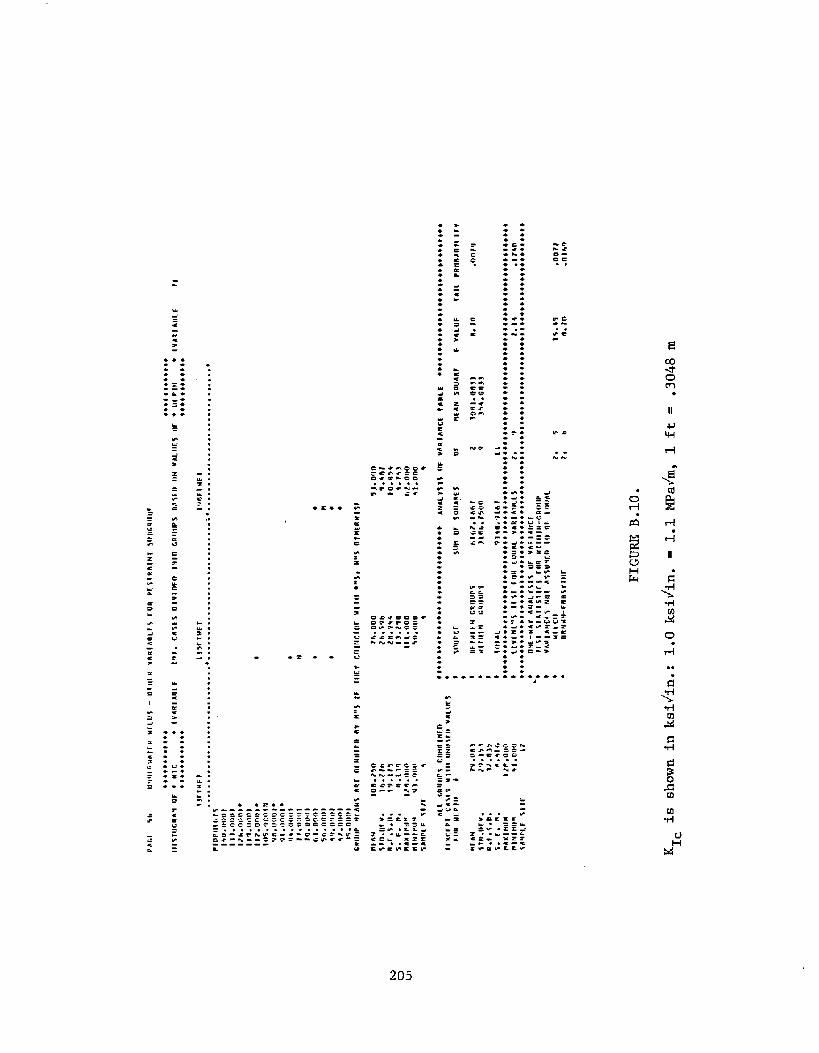
*::::::::..:.;..*:.
.
i=.:.:...:.::..::-.
u.::::
:..“
:
.
:
:
.
:
.
.
:
.
.
.
.
*:
~:*.L.m.-.-.
.
:...
:..:.
::.
-.k.x.-.-.-,-.
wdR.II
G
.-.. .*****: :::
*..:..:...:●✎
✚
✚✎✎☛✎
✚✎✎✎
II
:*
i:=*J.
:E. .-..- Z:=>-.
:
0.l-l
. :.* ..-*-*.. .*. ..*.-*.
:-2
v
MH

Mom
PLGF 5t. IJMWRMAIER lFfLIFS - UINtR V* RlfiFIIE\ FOR WFT ttR@lll C SUn Ct!!IUP
************ ******O*****N15rUGfltlY l?F * KIC + lVARIAfi LE t~). casFI utvliwn IMin GROIIPS oA51iI m vml. IIEt UF * nfpw + 4YhQ#AFYLE 1$
+9*+*+*+**** ********+***
llFIUrl S15Fl Htl 19aFtuEI. . . . . . . . . . . . . . . . . . . . . . . . . . . . . . . . . . . . . . . . . . . . . . . . . . . . . . . . . . . . . . . . . . . . . . . . . . . . . . . . . *.......?
HIF)PII INISire. nnolJ57. o(lnl *z+ll.ll(tol225.0 {!4)1?Io. titlol18*5.01101ll+o. Floflllb5. ooal150. oonl**135.00IJI*l>u. oollllllo~.nnnl *qu. noov** M Nt5. oilol ● ●
ho. (loo) * **45.0001 + **]n. onul *15.tum9
GRnllP HFAt41 hRE DtHFFt FIF BY lln S IF ItIF? COIMCIOE tiltt! **fi FFn5 tll MERWISE
ql.03? flo. lb?b7.253 no. }*nhh.05* 7t. OhZ27*+56 IZ. r+l
/1 ?.000 252.000m. oon +1. ono
t! b
● ☞☛☛☛☛☛☛☞☛☞☛☛☛☛☛☛☛☛☛☛☛☛☛☛☞☛☞☛☛☛ ANAL Y\l S EIF VAR’[AFFCE tfiOLE*
***** ***************4**********
* SOURCE J1)FI EIF SOUARf S mF MEhN 10uAm E f Vituf IAIL PulFmhni LtrY
● 1 IFVAL hzooo. 5ono 1?*b* **#***b*************** **** ***********+**+*********** ** ***+*+***********+******+*** **+****b. LEVCNf145 !E$[ Ftla EONAL VARIANCES 2, 15 1.1? .3317***** ************4******+**++ ***4*********+*********+ ****a ***** ***** **** D**** *t*************
* VMtl#~CES-Nnl ~sSNH[U lrF BE EOUflL+ IN l_cM* RROltN-rnll SY?NF.
FIGURE
K~c is shown in ksi~: 1.0 ksi~. = 1.1
1, n .02 .4 72YI?, 11 .11 .hl#7
B.Il.
MPa~, 1 ft = .3048 m

. . . . . . . . . . . . . . . . . . . . . . . . , . . . . . . . . . . . . . . . . . . . . . . . . . *. . . . . . . . . . . . . ...*.... . . . . . . . . . . . . . . . . . . . . .
rwfirl!IU. UEW.n.r.5, n.!. 1. If.PIfixl HUHr!twl1411HSAHPI E llr!
+
N
H
●
+4*+** **4** ****4 **4** 4******** *4 AtiiM.v51s rw vfi RI AwcF
. . . . . ...*
H*●*
5>. OUOT. 4111
10. nl+4.r+3
Liz .000$a. ono
4
***+* ***** 44**#***4****4 ********
● lull Wficl Irrrl l?ll. tl,ni* [uutta
t9f.1.5olt . fib .%lrnmool. f!uo t; )000. 1410
***** ***** b**** ***** **+* b** ****4 +**** +*4* **4********* *** D**** **4 b**** ***4 #*** ***** **+ ****4++
* vARt ANtFs rlol hsslmln 111 nf fuuAL* MILr,ll 5. 4 1*. YI* nuflluM-Frrn5vrllt
.001s5, 7 .nr .61?1
FIGURE B.12.
K~c is shown in lcsi~: 1.0 ksf~ = 1.1 MPa&, 1 ft = .3048 m, 1 in. = 25.4 mm
.—. —... ... ,.-.—.

woco
. . .. . . . . . . .. . . . . . . . . . . . . . . . . . . . . . . . . . . . . . . . . . . . *. . . . . . . . . . . . . . . . . . . . ...*... . . . . . . . . . .. . . . . . . ...*HIOP!IIWJ1
zl~. 4111*$155.00111 e?Go. urln)??5. unn)ztrr.w.in I H!.1%. UirallIno. uoot#1m5.<ln,ll
I
K~c is shown in
***** ********+*************.*** nMALY5t5 m vhRlmcc fnnl~*
**#** +***************+*********
4 %Wl!cc fun m Sal$hars rrr+
ur4r4 SmIM*F f Vtluc IAIL P#nnanlt Irv
FIGURE B.13.
ksi~: 1.0 ksi~ = 1.1 MPa&, 1 ft = .3048 m, 1 in. = 25.4 mm
— ......-–....+..,,>.>..>.s+.,._.-..______

************+ Dcpt$# 40 Inuf ●
*** be***+***
. . . . . . . . . . . . . . . . . . . . . . . . . . . . . . . . . . . . . . . . . . . . . ...*.*.. . . . . . . . . . . . . . . . . . . . . . . . . . . . . . . . . . . . . . . . . . . . . . ...+Hufrnlwf>
*
m
*
l? O.l, hFlo.n~ll14.111l#. nlb
15+. aooql.m!r
I
Culllclof UIlll +-1.
N
●
●
M-S UTltFn U15E
bM4
5’?. iloftIn. orroIn. +?oIn. Wttr, mo● 1 .000
1
Atl V,Rllll@l CIIHI14P3CIS **** ***+*********************** 4NL1v I!S OF VARI*WCF lAmLEttKCFPl cA51% !3111! UMOWII WALUFS *
dldll10NE
Inl. wohll, 1?15,1. J’thI+.?!*
/52 .000wt.*o(l
10
l?l. 1)1111.1?0133.115
r15.4#3252. rEoo
50.000I
● ********+++*******************
FIGURE B .14.
K~c is shown in ksi~in. : 1.0 ksi~in. = 1.1 MPa~m, 1 in. = 25*4 ~

● CVN
When CVN and percent shear are grouped by depth,
there is “no apparent effect. CVN showed no apparent
effect for zone, although there was greater variance
among the HAZ results. The 25.4 (1 in.)-thick welds
appeared to have lower CVN and percent shear, and
this effect was consistent at all depths. All of the
above conclusions
Figure B-15 shows
was the case for
are only half true, however.
CVN grouped by depth and zone. As
KIC (Figure B-14), the weld metal
toughness decreases with depth and exhibits little
variance, while the HAZ toughness is extremely high
and low with great variance and an apparently
constant mean with depth. Figure B-16 shows the
fracture appearance (percent shear) for the same
groups. Note that all the weld metal specimens were
full shear, and the HAZ specimens had mixed fracture
appearances.
The thickness effect is also influenced
shown in Figure B-17. Among the
specimens, thickness has very
12.7 mm (1/2 in.) HAZ specimens
all the rest, but for specimens
in.) welds, the HAZ toughness
by zone, as
weld metal
little effect. The
are much tougher than
taken from 25.4
is much lower,
even than the corresponding 25.4 mm (1 in.)
metal specimens. Hence, the thickness effect
manifestation of a change in HAZ toughness
mm (1
lower
weld
is a
with
thickness. This is important because it confirms the
suspicious phenomenon observed in the JIC tests, and
the number of Charpy specimens is sufficient to
210

******4*****
13FIWT It5Fwl l15rlMtl*{AI lrrt,ll }thl
. . . . . . ...+ . . . . . . . . . . . . . . ..0.,...,,., . . . . . . . . . . . . . . . . . . . . . ...*. . . . . . . . . . . . . . . . . . . . . . . . . . . . . . ...*
* ** Nt4 *4**+ *
m*** 4* ** ** 1** +* ***** * ●
+ ++
*****M******
11, orm 2+. I%o Zz.lr)l 31.11! 18.150/.,lJ1 1~.s,l 1 Z.1z’1 I 1.15i
26.5nol.~11 11. t+5
1 .0%! .?J.l/kl 2.*orl t5. rr5* 1, 10? ?l. ?)6.rl+* 5. ?4.? .fitz Y. f154 .5%2 5.hlt
lq , Orm 54. imlrr Zr. !roo 1/.000 22 .43r50 52 .rrtro.?,1 .Wlo 7.kM10 t’4.45r?tJ ‘+.000
itI 5.000 f,. 000
1> 12 12 12 1?
fitk mrrw~ cIIr5nlu*o ***** ****+ #******e**** ********* aNmLY
.:●
✎✎
✚
✚✎☛
✚
✚
✎✎☛
✚✎☛✎
::.*:..:
.:.
::::::----
a===5===Cecc. . . .g:::
:
.●
. .. .
212

..::..::....::*.::..:.
. .. ::..*..-**C*● .=*: .*.● *. .:: .:. .:.L:- .-..-..*::
: :: .:.:::
. .*<-=. ::: 52: .“-am-... ...***S *.* .
c--a- .k-- .9’-. : .*::.=...?..----- :
.s - . ..-.
::****
.:.
izi.
.- .::W .● . *- ....*. *.* ..-=. .. **.=***.. II
.:..:.:...
*.:●☛●✎
✚✎ z. ~:=.&-.:...**
...
..::
$:-, .w- ,.- .-=.
“.:
0●
l-l.:*. . .
.-r.
-.- ..*?*.*.* . .
:..:
:. G
g
m:. .. . . .. ----:-=**=: -.
m+
213

●
assure statistical significance at
percent (as given in the analysis of
in Figure B-17).
less than .01
variance table
Figure B-18 shows that the “thickness effect in the
HAZ” is associated with brittle fracture in the 25.4
mm (1 in.) HAZ specimens. These 25.4 mm (l-in.) HAZ
specimens are the only specimens with a fracture
appearance less than full shear, with a mean percent
shear of 30 percent.
As was the case for the other subgroups, there was no
temperature effect on the Charpy results.
Tearing Modulus
The tearing modulus was fairly constant with depth,
but like KIC and CVN, exhibited interactions with
thickness and zone. Figure B-19 resembles Figures B-
13 and B-17, i.e., the 12.7 mm (1/2 in.) HAZ
exhibited very high tearing modulus, nearly twice as
high as the weld metal, while the tearing modulus for
25.4 mm (1 in.) welds was independent of zone and of
the same order as the 12.7 mm (1/2 in.) weld metal.
● Bendscore
The ductility of the welds “is measured with the
Bendscore, which decreased monotonically with depth,
as shown in Figure B-20. Thickness had no effect on
the Bendscore.
214

wFm
. . . . . . . . . . . . . . . . . . . . ...0... . . . . . . . . . . . . . . . . . ...*..... . . . . . . . . . . . . . . . . . . . . . . . . . . . . . . . . . . . . . . . . ..*
CVN is shown in in. :
W,bh7.?lrl.Izr.ZZ5
Ioo. ofloqn. rroo
Z* ..
********************* homrll
●☛
*●☛
II*****e++*4******
?0.0003Z.4W131 .7!1
h.5$5~E.oOn
‘ae V& RlaUCF IhlELf +* b+++* *+*** ****4 +++** ***+* m+* b
t Iqzza. 4454 55. ZI . m-ml* llvfl Ivsoh. tl?e I 1950!I. Itrn
I14!IRACIION56. nz
*9 bofl. oorlo I. non o
I*ban. oaoo; Ci?qnn Zlfi??. $lt, r
9%. Z9 ,nnno60 1$0. IWI
***** ***** **4 *************9 **+*********+************* **+44 +*4************************ *****+** lIvr. F4rl*5 1[11 FNII Eoom Vanin!ccfi 1. an Z*.41 .nnon++*** ** D* ***b**************** **** ******************44*** ***#* ***** ***4* 4**+? ****4**** +*#*4*B* OWF-UA1 *4Fht Y315 IIF Vhnlhocc4 IE$l 51* II STICS FNR HIJI!III-CR!NIP* 9irll MlcEs Mnl k55UHE0 lU m run Al,* HELcM 3* 25*
3h.’3l .oonir9nuuM-rnnsrrt4c 1. 23 131. J6 . 00EHI
1 in. = 25.4 mm
FIGURE B.18.

t
***********D
Ifz Iq. Ill IN. 1 lW.w i n NA[ WEL!f. . . . . . . . . . . . . . . . . . . . ...*... . . . . . . . . . . . . . . . . . ...*..... . . . . . . . . . . . . .
****4*******nrf Vtl.llfs IIF * lNICM *
* lfl Mf +************
1 IN.Iial
. . . . . . . . . . . . . . . . . . . . . . . . . .
***U* fr*4 **
4* *
***+* ***4* *+ b*4***********+4* ** htlhl Yin*
fcr wfiul Awcf lAn Lf **4*,
. ..*
W************, ****4******
*- L(ti!.MI.”~ IEII FOn FONfiL VAUIANr.Ll ), 14***** ** b*4 ****+*06+** **404 +**** 4**** *m+0**4** *****m+ UNF-UAV AN4L?IJ5 OF wti121fiOC[* Ilfr Z! fill $llcs FIIR UIIIIIEE-GROUP* Vhqlh NCf5 rNcl A5StOfE0 Tn nc rullhl+ UFLCI! Y. 3* nnnmv-fufli7f*4F ). 6
FIGURE B.19.
CVN is shown in in, : 1 in. = 25.4 mm
Z. 741 .Ontfrb**4*0+4* **** 0* ***# ***** ***4+ **4** 4**4 **
?.20 .nznkb.lo .02q F
--, -. -. .... . ,.

PAGE II (ttWtC*Mal ER vIILYIS - SE M!FICOR FEVt MET FE FIRIFIC SUFIGRIEIIP
***********4
tll%lflGkfiM !lF * UIF4il%CilR * 4VAlllh8LE HI. CASE$ O[wlorvv Itflo Gnnurs BASFO ON VAL41E5 nF******O*****
YIFIME1 I15FIWEI lqLIFIUEf
vMl hBtE ?1
. . . . . . . . . . . . . . . . . . . . . . . . . . . . . 4, . .,, . . . . . ...+... * . ., . * . ., ...*.,... . . . . . . . . . . . . . . . . . . . . . ...*MIOP01M15
11>. moollF15. nFlnl
qn .0001vt. nnoO**64. (Fn(EINrr. nooaIo. ooi!l *bhnaol5b.0001~~.oalll+z. onom?5. !IOOI20.000121.0001t~.oaot
r,mlF18cmFluP IVEAHS
mra FAlln. nEv.S. E.S. O.5. F. *.mnxlmunIYIHIHUFISAFIPLE IIFE
ARE DfNtlWU OY IV-S IF lt4Fr CatlfClnE ILllll
04. I’1111. *)O11.6++
b.ene9$.00071. awo
1/1.000
I
********+**** II EFIII +**********8*
FIGURE B.20.
CVN is shown in ft. : 1 ft = .3048 m

..
:,.::..:::.:::.“..::::.:.:....:..
:
.’:.
:..:..:::..:.
:
. .FZ:C
*=~:z
.
b
.:.::::+:*:.....:..:...s..
:.;:
‘&.:..z<...:..:..::..:*.::..:●. .
●
✚
✚
✚
✚●
✚☞
✚
✚
✚
✚✎
✚●✎☛☛
✚☛☛
s.:.***:..*--..:*:.*.
m.b.G*-..*M-.*-.-.h.-.::..:*.::..A.
● *=:-.*...:
218

● HVN
B.2.4
includes
As shown in Figure B-21, hardness exhibited a
peculiar behavior. The hardness for 35 III (115 ft)
deep welds was lower than that of the 10 m (33 ft)-
deep welds and 60 m (198 ft) welds, which were
approximately equal. This effect is significant at
about 1 percent and was independent of thickness and
zone; the latter is surprising considering that the
weld metal hardness was measured at the weld crown,
while the HAZ hardness was measured at the
midplane. This reduction of hardness at 35 m (115
ft) may be due to something unique about the welding
procedure at that depth.
Results for All Data
The usefulness of looking at all the data together
verifying the applicability of trends observed in the
subgroups.
● Temperature Effect
Figure B-22 confirms the independence of toughness
from temperature.
● Thickness Effect on Ductility
Figure B-23 confirms the independence of Bendscore
from thickness and also shows how the scores tend to
cluster in groups. Figure B-24 shows the
Bendscore with depth. The mean Bendscore
from 97 for dry welds, to 61 for wet-backed
’219
trend of
decreases
welds, to

+tELoi - CVU hfln PC IJllEh~ rlSfl ALL Ft4T&
***+**+***+*15). Cfi5ES ~lVllLE13 lt4f0 GROUPS llAff D llN V41UfS EIF * ltMP ● lvmqi AnLE
*********+**
60 WC $
I* I
. . . . . . . . . . . . . . . . . . . . . . . . . . . . . . . . . . . . . . . . . . . . . . . . . . . . . . . . . . . . . . . . . . . . . . . . . . . . ...*rrmmrtfcrs
111. rFnnlIZF!.0001Il*b. nlln)113.1)01)1in%. omll**
,In. nllol’41.!P0411*a4. nml)l ***tl. iloo t*In.nnn)**h3.0001*blh. noo)****** m**4~. Ooal****b *********+.?. OI?IJIM***35.000)4+*+*42a.0001 *****21. UOOI******* ***+*****14. nu411***
r.aon I********ojriooi
-t. ouo#GR!FIIP tlF4M!
tlFhPI$ltF. oF V.
●
**
I!******+**+************$**********● ****4*
m. F.l. D. 23.9rQS. E. H. Z.blbJ5bm9Hun 10b. noaHIFll HurF s.nonSfitlP1.E $IJE 76
43.olqZ1. qElo2!.1/5
#.?51*tk.000
6.000Ih
●+***+**+******************** **●
hFIALrsls OF vAm
* \ouncE Zlln EIF fOUA#ES●
~F
* EIEIUEEM GaOUPS 29a. *ao3*
1ulr!lln GROUPS Rl~42.61n+
*190
&NcE tAn LE’ 4+++* #at****++*’ B*+** +4+4++++*?
* . Iotm n*241. oqn# 151***** **0* ***** ***** ***** ***** *m*** ***** **@** ***** ***** ***** ***** ***** ***** +**** *******4****** LE*EPJE-$ IESI FOk EOUiL VARlit4CES 1, 1>0 .05 .3)10***** **4** ***** ***** ***** ***** *#*4* ***u******** 6*9*, *+*** ****4+4*4*.,,*,,,,.,****,+,,,,,**+** iWff-Ufi Y AMILv51S ISF VASIAtlCE● 1[S1 Slh115Tl CS F4FR Wttl+l N-GROUPe VfiUIAHCES HnT aSSUMEO IU RE FotOhL* +lELCt!* BEl_EMt4-FwR$Yl!lF
1, 1501, 150
FIGURE B.22.
CVN is shown in ft-lb: 1.0 ft-lb = 1.356 J, “F = 1.8° C + 32
.4663
.4bh3
.,—?. ,-. . . . ... .... . . . . .

*O. VIIV2*.64331.618
fl. mlfl,)4.000
n.000tl
* +*******++****************** ** AwM.vS15 FFF Vfi RtAMIT lAn LE **+* O**** ********t****** *+*+***** SNFIRCF $4JM (EF 5011AlIr5 nF rllhfl snuAJrE F vnr-m IAIL pnorianatarv* -.* orr#r FF4 C-nu?s .113,) I . 115* . nn .9s?1* 1411111w GRINI?5 19055, ?n*l Ir 11.20 .q2n5** ~q[h~ l*056. orrm) in***** ***** ***** ***40 *****4***** ******************4*** ****# ***** *** O**** ********************e* Lrvrt4r~f IFfr Fon rotmt rfiRlm4ct5 I* 17 .?.59 .I?n?*+* #*************m**** *O******+************** ****a ***** ***a* ***m**** ***4************+******** NNr-W~? *NALfl15 (If Vh@l#NCE* * Irsr SIAI1511CS Fon !ll Tt41F4-wJroiIo* u#RlatlcFJ Nnr hlSNHEfl 111 Ok l~jllfil* wr.L r.4t 1, II . on*
. ~avr.IIrt NUP4-FNa JY rrir 1* II . on .~n~h
FIGURE 3.23.
CVN is shown in in. = 1 in. = 25.4 mm

.*::.*-=.:::*C**.*. .. ..**.:. .. .
:::-. ::!.:----*.. .. .::::::::. .. .. ... :.-..:**.*-*.- *E:. *-w..*. ..-**. ..-
....:..
-:;: .u.=,::
....
.
.
.-:~.
z:L.k-.-.-.
..:.::...-.
w.::s:-.
“.....
....z.w..?.=.-.
k:..:.
::.:.
.=.
.*2.
*. ● Z
●.x
Is● ✍✎☛ ✍✎.-..-..*
.
#:::=.+.=:~:=.-.-. II
.-* -.*.--**-* -----
i-l
● ☛
uw. . .
&:e:.=.
. -u.*W.7:::.::=:.-c.c ..+
.5
-:
222

56, 49, and 30 forwet weldsat 10, 35, and 60m (33,
115, and 198 ft), respectively. The minimum for wet-
backed welds is the 12.7 mm (1/2 in.) ferritic, and
the two smallest for the 10 m (33 ft) depth were both
austenitic. Obviously, these welds were not suitable
and they can be considered misapplications.
Disregarding these three, the minimum Bendscore
decreases from 94 for dry welds, to 65 for wet-backed
welds, 70, 45, and 23 for wet welds at 10, 35, and 60
m (33, 115, and 198 ft), respectively.
‘IC
Figure B-25 shows KIC g rouped by depth and zone. The
zone grouping was used to eliminate the extraordin-
arily high 12.7 mm (1/2 in.) HAZ values. Focusing on
weld metal K1C7 the mean decreases from 220 MPa/~
(200 ksi~~) for dry welds, to 187 MPa/~ (170
ksi/fi.) for wet-backed welds, and to 143, 58,
54 MPa/~, (130, 53, and 49 ksii~) for wet welds at
10, 35 and 60 m (33, 115, and 198 ft), respectively.
The minimum ‘Ic decreases from 149 MPa/~ (136
ksi~in.) for dry welds, to 89 MPaJfi (81 ksi~~) for
wet-backed welds, and to 107, 33, and 45 MPa/~ (97,
30, and 41 ksiJin.) for wet welds at 10, 35, and 60 m
(33, 115, and 198 ft), respectively.
● Thickness/Zone Interaction for Toughness
Figures B-26 and B-27 show the thickness/zone
interaction for CVN and KIC, and the results for all
data are consistent with those observed for other
223

Phlx Iar Rw.Y5tf m NtmwmII R wu)5 - E31wm wrlmcf InR JLL trnln
● *b********* ***+*+*+****untmwntior - KIC * !vARlfiu[r t~t. cri; fs rrlvltwtr Irm Cm ImFI ohwn m wnLiJEs rrr * rtr PIN * lvfit14nLE
*******4*+**rb
* lrtwF * !VMI ml.~ 2}1#**** ****9*#
oar EraT w rnrncu ME$trficK I!rl Hrl Ilrrwrl ll+Fl14tf 115Fl Wft l~nrfwEF t911rlUEFWFLfl Iml ur~ o Mhl U[LD IIA1 u r~ II t$fir Wr t N It& t. . . . . . . . . . . . . . . . . . . . . . . . . . . . . . ..*...... . . . . . . . . . . . . . . .! . . . . . . . ...* ., . . . . . ...* . . . . . . . ...) . . . . . . . . . . . . .,. ,.. . ..t
u
**
H
●
●
**
*rr●
*
*n*
N

..●✎✎✎
✚✎✎
✚✎
✎
✚✎✎✎
z“ :---9.-=.●....●....:..:.
.==:-.-% :..:...:....●..
<:-.-M :.- .-=..
:...:...::
:....
::
●✚✚✎ ✎ ✚✚✚✚✎ ✎ ✎✎✎ ✎✎✎✍✍✍✍✍✎☛☛☛✎✎☛✝✍✎● ✎
.In
.
*.:
.--m.*- .---
.
.●✎
✚
☛ ✚✎● ●✚
✎✍✚✎✎ ✍
✎ ✎ ✎ ✎ ✎☛☛☛☛☛✎✎ ✍✎☛☛✎✍☛✎✝✎☛☛ .
r*
*.*-● ✎. .
:--...**. =. :-....
...:.:
*:.

MC.Jm
pficr 5nr ArIhIr515 IIr UutnlunuhrtwUIC05- Ilrtltn vhulhntts IIIH Att N61n
*b*** b*** *e* *4**4**e ***b
ll15TNGltnH nr I H Ir. * 4Vh RIAOl F 171. ch$[f !)lvtrwn Ir4111 rJEIIUPS nnJIn w VAI. UIS OF * IUICH t***+*4****** + Iflfl E +
*********#**
ti) JJ4. 1/) Ill. 1 IN. I 114.Hiiu 186! U( Lu blat. . . . . . . . . . . . . . . . . . . . ...+ . . . . . . . . . . . . . . . . . . . . . . . . . . . . . . . . . . . . . . . . . . . . . . . . . . . . . . . . . . . . . . . . . . . . .
.
*#*●
H b
* *
flF hw 1+1 ,Wnsvn. nrv. r~.551*.r. s.n. H1. rlhlf. F. *. In.lz-l
aLL mlr411P5 C-trmllllwoIFw.*Pt chm dIIII Ntw1411 vmurs
Fll!r INICH atw turl( 1
*
H++**
..*
************+*************+** #* atmivill UF VLUlfir4C[ rAll LF4
**a **************b*************
* srlllrc E sun IIF sauA#f 5 nr#
HEWI SOOARr F V*lltF 14fL Pnrvnfintttrv
+ 1!11 cm Jlls?, aoln 1 33r5z. en3a*
V.h*10NI 15.?* t.lnl!I 1
.011715zf12. le19 1.15 .Onrll
6 wrkehctld~n lf, hhO. 011, h I lhhhO.03hh 1.55 .nhfl?+ [ IrqlJll 1’!4!684.110,11 )+ 4h,lh. t,1517***** **4m**b *m#***b $+***** i**** +m *4********************** ***** ***** ***** **+** **+** a*********
FIGURE 13.27.
.
‘Icis shown in ksi~in.: 1.0 ksi~in. = 1.1 MPaJm, 1 in. = 25.4 mm

groups, i.e. , the 12.7 mm (1/2 in. ) HAZ specimens
show higher toughness than both the HAZ and weld
metal 25.4 mm (1 in.) specimens and the 12.7 mm (1/2
in.) weld metal specimens.
227

APPENDIX C
Example 1: .Design of a Pipeline Repair
Problem: A 305 mm (12 in.) diameter 6.4 mm (1/4 in.) thick
pipeline riser requires a wet-welded sleeve to
cover and seal a hole about 76 mm (3 in.) long.
The yield strength of the pipe is 345 MPa (50
ksi) .
Considerations: The repair must be leak proof, therefore details
to limit crack size are unnecessary because
“failure” or leaking will occur upon crack
initiation. Therefore a more conservative
approach than usual will be adopted when designing
against crack initiation. The “second line of
defense”; i.e. crack arrest and/or redundancy,
which may preclude instability or collapse, does
not preclude leaking.
Solution: A simple full encirclement split sleeve is
chosen. The sleeve requires two longitudinal
groove welds and a circumferential fillet weld to
close each end.
1. The thickness of the sleeve is chosen to
ensure full section yielding of the pipeline
before yielding of the weld. A-36 plate is
chosen for the sleeve. Conservatively
assuming a yield strength of 248 MPa (36 ksi)
for the sleeve and uniform stress through the
thickness

F (pipeline)t
sleeve = Fy (sleeve) ‘pipeline
= ~~ $; (o.25 in) = .35 in.
use 9.7 mm (3/8 in.) thick sleeve.
2. Because the wet weld metal can be counted on
to have a strength greater than 345 MPa (50
ksi), the weld can be detailed normally, i.e.
per governing code such as AWS rules.
3. Check maximum stress in
fracture. The critical
longitudinal weld. Assume
the weld for
location is the
the load is high
enough to yield the pipeline, therefore the
stress in the groove weld is about 248 MPa (36
ksi) not considering the weld reinforcement.
The critical crack
(3/8 in.) since
constitute failure
5.1:
a. The repair wil
size is less
any through
by leaking.
1 be subject
than 9.7 mm
crack would
From Table
to a 4 hour
hydro test at greater than operating
pressure. This proof test will screen out
cracks larger than a given size that would
cause failure. However, to prevent
failure in the proof test, assume no
control of crack size: factor on crack
length = 4.0
{
,
229.:
,
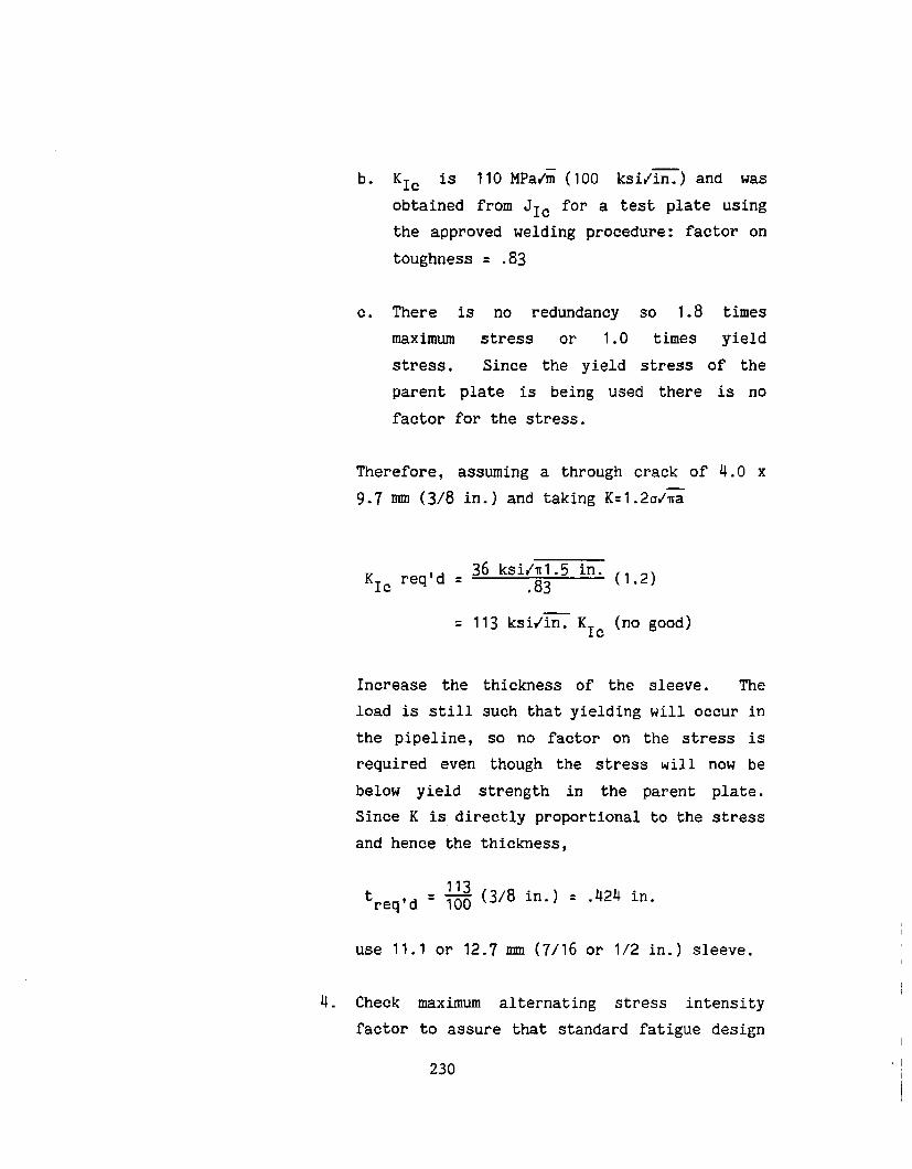
b. ‘Ic is 110 MPa/= (100 ksii~) and was
obtained from JIC for a test plate using
the approved welding procedure: factor on
toughness = .83
c. There is no redundancy so 1.8 times
maximum stress or 1.0 times yield
stress. Since the yield stress of the
parent plate is being used there is no
factor for the stress.
Therefore, assuming a through crack of 4.0 x
9.7 mm (3/8 in.) and taking K=l.2u/~
36 ksi4~l.5 in. (I ~,‘Ic
req’d =.83
.
= 113 ksi/~K,A (no good)
Increase the
load is still
the pipeline,
required even
Au
thickness of the sleeve. The
such that yielding will occur in
so no factor on the stress is
though the stress will now be
below yield strength in the parent plate.
Since K is directly proportional to the stress
and hence the thickness,
t113
req’d =~ (3/8 in.) = .424 in.
use 11.1 or 12.7 mm (7/16 or 1/2 in.) sleeve.
4. Check maximum alternating stress intensity
factor to assure that standard fatigue design
230

rules are applicable. Alternating stress
arises from being. downstream of a compressor
and from vortex shedding on the riser. The
maximum alternating stress range is 41.4 MPa
(6 ksi).
AK= 1.2
which is
The stress intensity range is:
6 ksi/~.375) = 7.8 ksid~.
well below 33 MPa/= (30 ksi/in.) and
in the regime where fatigue crack growth would
be much slower in the underwater weld than in
the base metal.
231

Example 2: Design of Strip Patch Repair for Sheet Piling
Problem: In order to carry the load across a split in some
sheet piling, it has been determined that 12.7 mm
(1/2 in.) thick 102mm (4 in.) wide plates will be
welded across the split on 0.61 m (2 ft) centers
as shown in Figure 5.4. For the plates, Fy is 248
MPa (36 ksi).
Considerations: The sheet piling is holding wet soil, so the
problem is to keep a split on some sheet piling
from getting wider and the repair does not have to
be water tight.
Solution: 1. Use fillet welds along the sides of the plates
to rely only on shear stress. The rated
strength of the E6013 electrodes is 414 MPa
(6o ksi).
2. Determine the length of plates required. The
effective throat distance for the fillet welds
is:
t= (.7o7) (1/2 in. - l/16 in.) = .3 in.
recognizing some weld throat loss due to “suck
up”, use t=.25 in.
Fv = 0.225 (6o ksi) = 13.5 ksi
The strength of the welds is therefore
f = 13.5 ksi . .25 in. = 3.37 k/in.
232

Design the fillet welds so that the plate can
be fully yielded before the shear stress in
the fillet welds approaches Fv.
Force in plate at yield . 36 ksi (4 in.) . 0.5 in. . 72 k
72 kE
req’d = 3.4 k/in = 21 in.
Assume the gap is less than 51 mm (2 in.)
wide, then use plates 610 mm (24 in.) long
with 267 mm (10.5 in.) long fillet welds on
each side.
3. Fracture is not a problem because of the
reliance solely on shear stresses and the high
degree of redundancy (number of patch plates).
4. Fatigue from alternating stress is not a
problem.
233

Example 3: Design of a Replacement of Damaged Tubular Brace
Subject to Tension
Problem: The brace is cracked at the weld to the spud
can. The spud can is not damaged, so the brace
will be cut away and a replacement component will
be fit and attached to the brace with a doubler.
The replacement component will be shop welded in
advance to half a sleeve which will be attached to
the spud can, see Figure 5.1. The spud can is 305
IMKI (12 in.) in diameter and 12.7 mm (1/2 in.)
thick. The original brace is 254 mm (10 in.) in
diameter and 12.7 mm (1/2 in.) thick. Both
components have a yield strength of 345 MPa (50
ksi) .
Considerations: The brace can be put into significant tension
when structure is subject to wave loading.
Therefore, the use of details to limit the crack
size are warranted since the brace is deemed
critical.
Solution: 1. The brace connection should use a scalloped
full encirclement split sleeve (Doubler B in
Figure 5.1) to maximize weld length and area,
and to utilize shear stress as much as
possible to transfer the axial load. The
connection to the spud can (Doubler A in
Figure 5.1) should use an interlocking full
encirclement split sleeve doubler to transfer
axial load from the brace through contact on
the opposite side of the spud can. Since the
longitudinal weld of this split sleeve will
234

still have to support tension, circumferential
fillet welds are used on the ends to provide a
redundant load path. The weld is to be made
in shallow water (depth of 10 m (33 ft)) and
since higher carbon equivalent base plate is
to be welded, austenitic electrodes are
selected. The rated strength of the electrode
is 552 MPa (8o ksi), so the allowable stress
is .225 the rated strength or 124 MPa (18
ksi) . The toughness of the weld is 253 MPa/~
(230 ksii~) which was obtained from a
correlation to the Charpy toughness.
2. Size the split sleeves. Use a replacement
brace component the same size as the original
brace to minimize stiffening of the joint.
The shop weld is designed under the governing
code, e.g. AWS rules, and is not considered
here.
Doubler B:
1. Try a 19 mm (3/4 in.) thick sleeve with FY=248
MPa (36 ksi). The scalloped sleeve has a
total circumference of 838 mm (33 in.) but an
arc length of weld of 1575 mm (62 in.) on
either end. Take 838 mm (33 in.) as being in
tension and 737 mm (29 in.) in shear. The
throat for the 19 mm (3/4 in.) leg fillet weld
is:
.707(.75-.06) - .12 = .37 in.
235
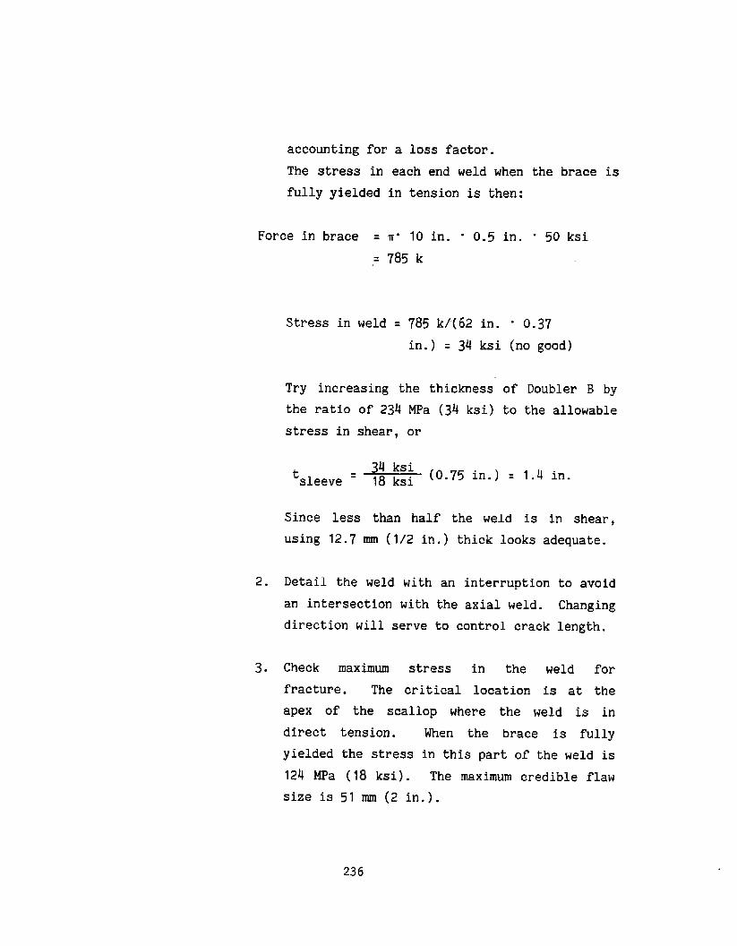
accounting for a loss factor.
The stress in each end weld when the brace is
fully yielded in tension is then:
Force in brace = m- 10 in. - 0.5 in. “ 50 ksi
= 785 k
2.
3.
Stress in weld
Try increasing
= 785 k/(62 in. - 0.37
in.) ❑ 34 ksi (no good)
the thickness of
the ratio of 234 MPa (34 ksi) to
stress in shear, or
t34 ksi
sleeve = 18 ksi(0.75 in.) =
Since less than half the weld
Doubler B by
the allowable
1.4 in.
is in shear,
using 12.’7 mm (1/2 in.) thick looks adequate.
Detail the weld with an interruption
an intersection with the axial weld.
direction will serve to control crack
to avoid
Changing
length.
Check maximum stress in the weld for
fracture. The critical location is at the
apex of the scallop where the weld is in
direct tension. When the brace is fully
yielded the stress in this part of the weld is
124 MPa (18 ksi). The maximum credible flaw
size is 51 mm (2 in.).
236

From Table 5.1:
a. Changed direction into shear stress, and
maximum flaw size is less than the
continuous length of weld. The factor on
crack length is therefore 1.6.
b. The toughness
test, use a
toughness.
c. The structure
factor of
appropriate.
Stress analysis
was estimated from a Charpy
factor of 0.67 on the
is highly redundant, so a
1.2 on the stress is
reveals that the stress
concentration factor for this geometry is
2.0. The maximum K is then:
‘Icreq’d ❑ (2.o) (1.2) 18 ksi/~(1.6)2/.67
❑ 137 ksi/~/.67 = 204 < 236
Doubler A:
The
the
the
chord is in compression from dead load, so
critical load for fracture of doubler A is
axial tension in the brace. The split
sleeve will have two longitudinal groove welds
subject to tensile or hoop stress. Since the
maximum credible flaw size is the same, i.e.
S1 mm (2 in.), try a 19 mm (3/4 in.) doubler
sleeve. It is now known that the stress must
be kept below 124 MPa (I8 ksi) to tolerate
237

this flaw, so calculate the length of the
doubler:
785k!2req’d ❑ 18 ksi 0.75 in. ❑ 58 in.
Doubler A should be 1.5 m (5 ft) long.
Since circumferential fillet welds also hold
the doubler to the chord, this system is
highly redundant. Check maximum alternating
stress intensity for fatigue. Max imum
alternating
be 100k.
either weld
load in the brace is estimated to
The alternating stress range in
(Doubler A or B) is then.
1Ook— x 18 ksi = 2.3 ksi785k
The maximum range in stress intensity factor
is then:
AK = (2.0) 2.3 ksi#(2 in.)
= 11.5 ksii~ < 30 ksii~
Therefore crack growth will be in the regime
where the crack would grow faster in the base
metal, and standard fatigue design procedures
are applicable.
238

BIBLIOGRAPHY
1.
2.
3.
4.
5.
-.
6.
7.
American Welding Society, “Specification for Underwater
Welding--AWS D3.6,” 1983, Miami, Fla.
Brown, A. J.; Staub, J. A.; and Masubuchi; K.,
“Fundamental Study of Underwater Welding,!’ 4th Annual
Offshore Technology Conference OTC 1621, April 30 - May 3,
1972.
Brown, R. T., and Masubuchi, K., llFundmental Research on
Underwater Welding, “ WeldinR Journal, Vol. 54, No. 6, June
1975.
Burner, W. K., “Generalized Summary of the State-of-the-
Art of Underwater Welding,’! Naval Engineers Journal.
April 1978, pp. 68-74.
Dadian, M., “Review of Literature on the Weldability
Underwater of steels,” Welding In The World, Vol. 14, No.
3/4, 1976.
Fukushima, T.; Fukushirna, S.; Kinugawa, J., “Some
Mechanical Properties of Multi-pass Welds by Underwater
Wet Plasma Welding,” National Research Institute for
Metals, Tokyo, Japan, 1979.
Grubbs, C. E., and Seth, O. W., “Underwater Wet Welding
with Manual Arc Electrodes,’f Published in Underwater
WeldinE for Offshore Installations, The Welding Institute,
Abington Hall, Abington, Cambridge, 1977.
239

8.
9.
10.
11.
12.
13.
14.
15.
Hamasaki, M.; Sakakibara, J.; and Arata, y., “underwater
Wet Welding and Hydrogen, ” Metal Construction, December
1981, pp. 755-756.
Helburn, S., “Underwater Welders Repair Drilling Rig,’t
welding Design & Fabrication, July 1979.
Madatov, N. M., “Energy Characteristics of the Underwater
Welding Arc,” WeldinR Research, Vol. 13, No. 5, May 1967.
Masubuchi, K., and Meloney, M. B., “underwater welding of’
Low-Carbon and High-Strength (HY-80) Steel,’! Offshore
Technology Conference, OTC 1951, 1974.
Military Standard: Underwater Welding Requirements for
Naval Facilities, MIL-STD-1692 (YD) February 1976.
Nagarajan, V., and Loper, C. R., “underwater welding of
mild Steel-A Metallurgical Investigation of Critical
Factors,” Offshore Technology Conference, Houston, Texas,
OTC 2668, 1976.
Sadowski, E. P., “Underwater Wet Welding Mild Steel with
Nickel Base and Stainless Steel Electrodes,” Welding
Journal, July 30, 1980, pp. 30-38.
Shinada, K.; Nagata, Y.; Wada, H., Tamura, M.; Mae, T.;
Manabe, Y.; and Nobushige, T., “Development of Underwater
Welding Techniques,” Technical Review, Mitsubishi Heavy
Industries, Vol. 16, No. 2, Ser. No. 45, June 1979.
240

16. Stalker, Q. W., “Welding Institute Research on Underwater
Welding,” Published in Underwater Welding for Offshore
Installations, The Welding Institute, Abington Hall,
Abington, Cambridge, 1977.
17. Stalker, A. W.; Hart, P. H. M.; and Salter, G. R., ‘tA
Preliminary Study of Underwater Manual Arc Welding,” The
Welding Institute, Abington Hall, Abington, Cambridge,
December 1974.
18. Stalker, A. W.; Hart, P. H. M.; and Salter, G. R., !!An
Assessment of Shielded Metal Arc Electrodes for the
Underwater Welding of Carbon Manganese Structural Steels,”
Offshore Technology Conference, OTC 2301, Houston, Texas,
May 5-8, 1975.
19. Tsai, C. L., and Masubuchi, K., “Interpretive Report on
Underwater Welding,” Welding Research Council, Bulletin
No. 224, February 1977.
241
, .,.,,,,,..