SSA SWE TWO NEW PRECURSOR SERVICES - TECHNICAL NOTE...
43
EUROPEAN SPACE AGENCY DIRECTORATE OF OPERATIONS AND INFRASTRUCTURE OPS-GI SSA SWE – TWO NEW PRECURSOR SERVICES - TECHNICAL NOTE 2 DESCRIPTION OF THE ALGORITHMS AND THE MATHEMATICAL FORMULA- TION FOR BOTH NEW PRECURSOR SERVICES Reference: SSA-SWE-SWEP-TN-0003 Version: 1.1 Date: 24 February 2014
Transcript of SSA SWE TWO NEW PRECURSOR SERVICES - TECHNICAL NOTE...
EUROPEAN SPACE AGENCY
DIRECTORATE OF OPERATIONS AND INFRASTRUCTURE
OPS-GI
SSA SWE – TWO NEW PRECURSOR SERVICES - TECHNICAL NOTE 2
DESCRIPTION OF THE ALGORITHMS
AND THE MATHEMATICAL FORMULA-TION FOR BOTH NEW PRECURSOR
SERVICES
Reference: SSA-SWE-SWEP-TN-0003
Version: 1.1
Date: 24 February 2014
EUROPEAN SPACE AGENCY
DIRECTORATE OF OPERATIONS AND INFRASTRUCTURE
OPS-GI
VERSION: 1.1 - 24 FEBRUARY 2014 I / VIII © COPYRIGHT EUROPEAN SPACE AGENCY 2012
Document Title: SSA SWE – Two New Precursor Services – Technical Note 2: Description of algorithms and their mathematical formulation for both new precursor services
Document Reference: SSA-SWE-SWEP-TN-0003
Document Version: 1.1 Date: 24 February 2014
Abstract
Approval Table:
Action Name Function Signature Date
Prepared by: Ralf Keil Project Manager 24 February 2014
Verified by: Pablo Beltrami Technical Consultant 24 February 2014
Approved by: [Vicente Navarro] ESA Technical Officer <<Authorised On>>
Authors and Contributors:
Name Contact Description Date
Ralf Keil [email protected] Author 30 September 2013
Kirsti Kauristie [email protected] Contributor FMI 25 September 2013
Philippe Yaya [email protected] Contributor CLS 27 September 2013
Yannick Béniguel [email protected] Contributor IEEA 06 September 2013
Louis Hecker [email protected] Contributor CLS 27 September 2013
Distribution List:
© COPYRIGHT EUROPEAN SPACE AGENCY, 2012
The copyright of this document is vested in European Space Agency. This document may only be reproduced in whole or in part, stored in a retrieval system, transmitted in any form, or by any means electronic, mechanical, photocopying, or otherwise, with the prior permission of the owner.
Document Change Log
Reason for change Issue Revision Date
Draft version 0 1 06 August 2013
First release 1 0 30 September 2013
Implementation of CDR RIDs 1 1 24 February 2014
Document Change Record
DCR No: 0001 Originator:
Date: Approved by:
Document Title: SSA SWE – Two New Precursor Services – Technical Note 2: Description of algorithms and their mathematical formulation for both new precursor services
Document Reference: SSA-SWE-SWEP-TN-0003

SSA-SWE-SWEP-TN-0003 TECHNICAL NOTE 2: DESCRIPTION OF ALGORITHMS
VERSION: 1.1 - 24 FEBRUARY 2014 II / VIII © COPYRIGHT EUROPEAN SPACE AGENCY 2012
Page Paragraph Reason for Change
4f. 3.3 RID #107: added more text on alert thresholds
33 B.3 RID #108: ACE alerts explained in more detail; link from AurorasNow! service to FMI/ACE alerts clarified
7 3.6.3 RID #109: added an explanation of a potentially large difference between the model and the magnetometer data
9f. 3.6.4 RID #110: updated description of the Blinking lamps mechanism; Tlamp parameters removed
9ff. 3.6.5 RID #111: added an explanation of the *) marking; added a description of an approach to handle cases of too few data points (strong activity)
III – IV, 16, 18, 26 - 28, 30
Table of Content, Table of Figures, Table of tables, 4.2.3.1, 5.3.2, 5.5
RID #112: remove non-headers from doc map
Title RID #120: change doc title
SSA-SWE-SWEP-TN-0003 TECHNICAL NOTE 2: DESCRIPTION OF ALGORITHMS
VERSION: 1.1 - 24 FEBRUARY 2014 III / VIII © COPYRIGHT EUROPEAN SPACE AGENCY 2012
TABLE OF CONTENTS
1. APPLICABLE AND REFERENCE DOCUMENTS ............................................................................. VII
1.1 APPLICABLE DOCUMENTS .................................................................................................................. VII
1.2 REFERENCE DOCUMENTS .................................................................................................................. VII
2. INTRODUCTION ...................................................................................................................................... 1
3. THE REGIONAL AURORA FORECAST .............................................................................................. 3
3.1 SCIENTIFIC BACKGROUND ................................................................................................................... 3
3.2 NOWCASTING AURORAL ACTIVITY FROM THE BASIS OF MAGNETIC RECORDINGS .................................. 3
3.3 FORECASTING AURORAL ACTIVITY FROM THE BASIS OF STATISTICAL RELATIONSHIPS ........................... 4
3.4 GETTING INFORMATION ABOUT CLOUDINESS ....................................................................................... 6
3.5 GETTING INFORMATION ABOUT THE SUN AND MOON RISE AND SET TIMES ........................................... 6
3.6 ALGORITHMS ...................................................................................................................................... 7
3.6.1 Determining the location of the auroral band based on dB/dt (Nowcast) .................................. 7
3.6.2 Determining the location of the statistical auroral oval based on Kp ......................................... 7
3.6.3 The algorithm for OvalMakerNow ................................................................................................ 7
3.6.4 Algorithm for BlinkingLamps ........................................................................................................ 9
3.6.5 Algorithm for OvalMakerFore ....................................................................................................... 9
4. THE IONOSPHERIC SCINTILLATION MONITORING ...................................................................... 14
4.1 IONOSPHERE OBSERVATION WITH GPS............................................................................................. 14
4.1.1 Pseudo-range or code observation ........................................................................................... 14
4.1.2 Carrier phase observation .......................................................................................................... 14
4.1.3 Geometry-free linear combination ............................................................................................. 15
4.1.4 TEC computation ........................................................................................................................ 15
4.2 ALGORITHMS FOR KEY PARAMETERS CALCULATION ........................................................................... 16
4.2.1 ROTI ............................................................................................................................................ 16
4.2.2 IndexDtDS1 ................................................................................................................................ 16
4.2.3 Single layer model ...................................................................................................................... 16
4.2.4 TEC Calibration .......................................................................................................................... 18
5. IONOSPHERIC SCINTILLATION MAPPING ..................................................................................... 20
5.1 INTRODUCTION.................................................................................................................................. 20
5.2 RAW DATA ANALYSIS ......................................................................................................................... 20
5.2.1 Introduction ................................................................................................................................. 20
5.2.2 Power Density Spectrum ........................................................................................................... 21
5.2.3 Under sampling effects............................................................................................................... 22

SSA-SWE-SWEP-TN-0003 TECHNICAL NOTE 2: DESCRIPTION OF ALGORITHMS
VERSION: 1.1 - 24 FEBRUARY 2014 IV / VIII © COPYRIGHT EUROPEAN SPACE AGENCY 2012
5.2.4 S4 comparison over one night of observation .......................................................................... 24
5.3 GISM MODELLING ............................................................................................................................ 25
5.3.1 Introduction ................................................................................................................................. 25
5.3.2 Comparison with measurements ............................................................................................... 26
5.4 INPUT DATA ....................................................................................................................................... 27
5.5 ALGORITHM ...................................................................................................................................... 28
5.6 EXAMPLE OF RESULTS ...................................................................................................................... 30
APPENDIX A URL ADDRESSES ............................................................................................................ 32
APPENDIX B ALERTS .............................................................................................................................. 33
B.1 NOAA ALERTS.................................................................................................................................. 33
B.2 SIDC HALO-CME ALERT .................................................................................................................. 33
B.3 FMI/ACE ALERT ............................................................................................................................... 33
SSA-SWE-SWEP-TN-0003 TECHNICAL NOTE 2: DESCRIPTION OF ALGORITHMS
VERSION: 1.1 - 24 FEBRUARY 2014 V / VIII © COPYRIGHT EUROPEAN SPACE AGENCY 2012
TABLE OF FIGURES FIGURE 1 ARCHITECTURAL DESIGN OF THE SWE WEB PORTAL AND ITS SERVICES WITH PARTICULAR REGARD
TO THE BPS AND SERVICES OF THE TWO NEW PRECURSOR SERVICES RAF AND ISM ...................................... 1
FIGURE 2 MAGNETOMETER STATIONS (RED CIRCLES) AND AURORAL CAMERA STATIONS (FIELD-OF-VIEWS
MARKED WITH ORANGE CIRCLES) PROVIDING NRT FOR RAF SERVICE. THE LOCATIONS OF HEL AND NYR
CAMERA STATIONS ARE MARKED WITH ORANGE DOTS. THE TWO OTHER CAMERA STATIONS ARE LOCATED IN
KEV AND MUO. ........................................................................................................................................................ 4
FIGURE 3 PROBABILITY TO RECORD DB/DT VALUES HIGHER THAN 0.57 NT/S IN KEV DURING THE 48 HOURS
AFTER THE ISSUANCE OF NOAA ALTK06 ALERT. ................................................................................................. 6
FIGURE 4 EXAMPLE PLOT FROM THE RAF NOWCAST PART. GREEN SHOWS THE LOCATION OF AURORAL BAND
AS DETERMINED FROM NRT MAGNETOMETER DATA AND CYAN SHOWS THE STATISTICAL AURORAL OVAL
MODEL (DEPENDENT ON KP VALUE). THE RED LINE SHOWS THE EQUATORWARD BOUNDARY OF THE DIFFUSE
OVAL. 8
FIGURE 5 QUIET TIME PLOT FROM THE RAF NOWCAST PART. THE GREY BAND SHOWS THE APPROXIMATE
LOCATION OF AURORAL OVAL IN CASE OF NO SIGNIFICANT ACTIVITY .................................................................... 8
FIGURE 6 AN EXAMPLE OF THE PLOTS WHICH WILL BE SHOWN ON THE FORECAST WEB PAGES. GREEN (CYAN) SHOWS THE LATITUDE BAND WHERE THE DB/DT THRESHOLD IS EXCEEDED WITH >0.7 (0.5) PROBABILITY. .. 12
FIGURE 7 FLOW CHART DESCRIBING THE SELECTION OF PROBABILITYCURVES FOR THE DIFFERENT
TRIGGERINGALERTS ............................................................................................................................................... 13
FIGURE 8 IONOSPHERIC PIERCE POINT .................................................................................................................... 17
FIGURE 9 SINGLE LAYER MODEL ................................................................................................................................ 18
FIGURE 10 1-MIN SAMPLE PHASE AND INTENSITY AND CORRESPONDING SPECTRUM ........................................ 21
FIGURE 11 P SLOPE SPECTRUM HISTOGRAMS OF INTENSITY AND PHASE SCINTILLATION .................................. 22
FIGURE 12 UNDERSAMPLING AT 1 HZ AND CORRESPONDING SPECTRUM .......................................................... 23
FIGURE 13 PHASE INDEX CALCULATION USING 50 HZ DATA AS COMPARED TO A 1 HZ DATA CALCULATION .... 24
FIGURE 14 S4 INDEX AND ROTI INDEX CALCULATED FROM 50 HZ AND 1 HZ DATA AT TWO CLOSE LOCATIONS
25
FIGURE 15 INTENSITY AND PHASE SCINTILLATION INDICES MEASUREMENTS ON GPS WEEK N° 377 .............. 26
FIGURE 16 INTENSITY AND PHASE SCINTILLATION INDICES ON DAY 314, GPS WEEK N° 377, OBTAINED BY
MODELING ................................................................................................................................................................. 27
FIGURE 17 THE VARIOGRAM FUNCTION OBTAINED BY MODELING (LEFT PANEL) PROVIDES A GOOD ESTIMATE
OF THE ONE OBTAINED USING THE MEASUREMENTS (RIGHT PANEL). ................................................................. 29
FIGURE 18 KRIGING SCINTILLATION MAP AND ESTIMATES ON A CUT AT ONE PARTICULAR LATITUDE VALUE .... 30
FIGURE 19 FMI/ACE ALERT TABLE AS SHOWN IN THE AURORASNOW! SERVICE (AURORA.FMI.FI). MIN(RX) AND MAX(RX) VALUES WHICH ARE USED IN THE RAF SERVICE ARE GIVEN IN THE 2
ND AND 3
RD COLUMNS OF
THE GEOMAGNETIC ACTIVITY TABLE. ..................................................................................................................... 34
TABLE OF TABLES TABLE 1 APPLICABLE DOCUMENTS ......................................................................................................................... VII
TABLE 2 REFERENCE DOCUMENTS ........................................................................................................................ VIII
TABLE 3 LIST OF DELAY TIMES WHEN THE PROBABILITY TO EXCEED THE DB/DT VALUE IS 0.5-0.7 (FIRST SUB-COLUMN) AND >0.7 (SECOND SUB-COLUMN) FOR EACH ALERT TYPE AND STATION. N/A MEANS THAT THE
THRESHOLD EITHER FOR 0.5 OR 0.7 IN THE PROBABILITY HAS NOT BEEN EXCEEDED IN OUR DATA SET. *) MEANS THAT LESS THAN 21 DATAPOINTS (FOR EACH TIMESTEP) WERE AVAILABLE FOR THE ANALYSIS. ........ 11

SSA-SWE-SWEP-TN-0003 TECHNICAL NOTE 2: DESCRIPTION OF ALGORITHMS
VERSION: 1.1 - 24 FEBRUARY 2014 VI / VIII © COPYRIGHT EUROPEAN SPACE AGENCY 2012
TABLE 4 INDICES AND PERIODS ................................................................................................................................ 16
TABLE 5 LIST OF URL ADDRESSES RELEVANT FOR THE RAF SERVICE ............................................................... 32
SSA-SWE-SWEP-TN-0003 TECHNICAL NOTE 2: DESCRIPTION OF ALGORITHMS
VERSION: 1.1 - 24 FEBRUARY 2014 VII / VIII © COPYRIGHT EUROPEAN SPACE AGENCY 2012
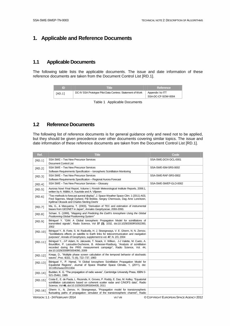
1. Applicable and Reference Documents
1.1 Applicable Documents
The following table lists the applicable documents. The issue and date information of these reference documents are taken from the Document Control List [RD.1].
ID Title Reference
[AD.1] DC-IV SSA Prototype Pilot Data Centres: Statement of Work Appendix I to ITT
SSA-DC-CF-SOW-0004
Table 1 Applicable Documents
1.2 Reference Documents
The following list of reference documents is for general guidance only and need not to be applied, but they should be given precedence over other documents covering similar topics. The issue and date information of these reference documents are taken from the Document Control List [RD.1].
Ref. Title Code
[RD.1] SSA SWE – Two New Precursor Services
Document Control List
SSA-SWE-DCIV-DCL-0001
[RD.2] SSA SWE – Two New Precursor Services
Software Requirements Specification – Ionospheric Scintillation Monitoring
SSA-SWE-ISM-SRS-0002
[RD.3] SSA SWE – Two New Precursor Services
Software Requirements Specification – Regional Aurora Forecast
SSA-SWE-RAF-SRS-0002
[RD.4] SSA SWE – Two New Precursor Services – Glossary SSA-SWE-SWEP-GLO-0002
[RD.5] Auroras Now! Final Report, Volume I, Finnish Meteorological Institute Reports, 2006:1, written by A. Mälkki, K. Kauristie and A. Viljanen
[RD.6] “Two methods to forecast auroral display”, J. Space Weather Space Clim. 1 (2011) A03, Fred Sigernes, Margit Dyrland, Pål Brekke, Sergey Chernouss, Dag Arne Lorentzen, Kjellmar Oksavik and Charles Sterling Deehr
[RD.7] Ma, G., & Maruyama, T. (2003), “Derivation of TEC and estimation of instrumental biases from GEONET in Japan”, Annales Geophysicae, 2093-2093.
[RD.8] Schaer, S. (1999), “Mapping and Predicting the Earth's Ionosphere Using the Global Positionning Global Positionning System”
[RD.9] Béniguel Y. "GIM: A Global Ionospheric Propagation Model for scintillations of transmitted signals", Radio Science, Vol 37 (3), 1032, doi:10.1029/2000RS002393, 2002
[RD.10] Béniguel Y., B. Forte, S. M. Radicella, H. J. Strangeways, V. E. Gherm, N. N. Zernov, "Scintillations effects on satellite to Earth links for telecommunication and navigation purposes", Annals of Geophysics, supplement to vol. 47, N. 2/3, 2004
[RD.11] Béniguel Y., J-P Adam, N. Jakowski, T. Noack, V. Wilken, J-J Valette, M. Cueto, A. Bourdillon, P. Lassudrie-Duchesne, B. Arbesser-Rastburg, “Analysis of scintillation recorded during the PRIS measurement campaign”, Radio Science, Vol. 44, doi:10.1029/2008RS004090, 2009
[RD.12] Knepp, D., “Multiple phase screen calculation of the temporal behavior of stochastic waves”, Proc. IEEE, 71 (6), 722–737, 1983
[RD.13] Béniguel Y., P. Hamel, “A Global Ionosphere Scintillation Propagation Model for Equatorial Regions”, Journal of Space Weather Space Climate, 1, (2011), doi: 10.1051/swsc/2011004
[RD.14] Budden, K. G. “The propagation of radio waves”, Cambridge University Press, ISBN 0-521-25461, 1985
[RD.15] Costa E., E. de Paula, L. Rezende, K. Groves, P. Roddy, E. Dao, M. Kelley, “Equatorial scintillation calculations based on coherent scatter radar and C/NOFS data”, Radio Science, Vol 46, doi:10.1029/2010RS004435, 2011
[RD.16] Gherm V., N. Zernov, H. Strangeways, “Propagation model for transionospheric
fluctuating paths of propagation: simulator of the transionospheric channel”, Radio
SSA-SWE-SWEP-TN-0003 TECHNICAL NOTE 2: DESCRIPTION OF ALGORITHMS
VERSION: 1.1 - 24 FEBRUARY 2014 VIII / VIII © COPYRIGHT EUROPEAN SPACE AGENCY 2012
Ref. Title Code
Science, Vol 40, RS1003, doi:10.1029/2004RS003097, 2005
[RD.17] Radicella S.M., “The NeQuick model genesis, uses and evolution”, Annals of Geophysics, Vol 52 (3-4), 2009.
[RD.18] J.J. Valette, P. Lassudrie-Duchesne, N. Jakowski, Y. Beniguel, V. Wilken, M. Cuerto, A. Bourdillon, C. Pollara-Brevart, P. Yaya, J.P. Adam, R. Fleury, “Observations of ionospheric perturbations on GPS signals at 50 Hz, 1 Hz and 0.03 Hz in South America and Indonesia”, European Space Weather Week, Brussels, November 2007
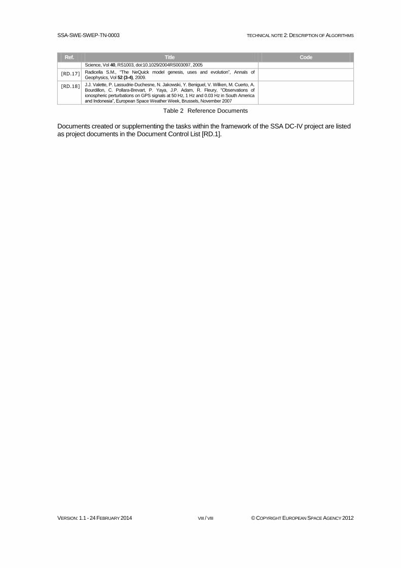
Table 2 Reference Documents
Documents created or supplementing the tasks within the framework of the SSA DC-IV project are listed as project documents in the Document Control List [RD.1].
SSA-SWE-SWEP-TN-0003 TECHNICAL NOTE 2: DESCRIPTION OF ALGORITHMS
VERSION: 1.1 - 24 FEBRUARY 2014 1 / 34 © COPYRIGHT EUROPEAN SPACE AGENCY 2012
2. Introduction
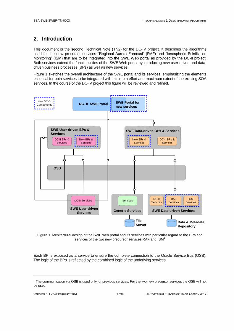
This document is the second Technical Note (TN2) for the DC-IV project. It describes the algorithms used for the new precursor services “Regional Aurora Forecast” (RAF) and “Ionospheric Scintillation Monitoring” (ISM) that are to be integrated into the SWE Web portal as provided by the DC-II project. Both services extend the functionalities of the SWE Web portal by introducing new user-driven and data-driven business processes (BPs) as well as new services.
Figure 1 sketches the overall architecture of the SWE portal and its services, emphasizing the elements essential for both services to be integrated with minimum effort and maximum extent of the existing SOA services. In the course of the DC-IV project this figure will be reviewed and refined.
OSB
Services
Generic Services
File
Server
ISM
Services
Data & Metadata
Repository
SWE Data-driven Services
SWE Data-driven BPs & Services
New BPs &
Services
RAF
Services
SWE User-driven BPs &
Services
SWE User-driven
Services
DC-II BPs &
Services
DC-II BPs &
Services
SWE Portal for
new servicesDC- II SWE Portal
DC-II
ServicesDC-II Services
New DC-IV
Components
New BPs &
Services
Figure 1 Architectural design of the SWE web portal and its services with particular regard to the BPs and
services of the two new precursor services RAF and ISM1
Each BP is exposed as a service to ensure the complete connection to the Oracle Service Bus (OSB). The logic of the BPs is reflected by the combined logic of the underlying services.
1 The communication via OSB is used only for previous services. For the two new precursor services the OSB will not
be used.
SSA-SWE-SWEP-TN-0003 TECHNICAL NOTE 2: DESCRIPTION OF ALGORITHMS
VERSION: 1.1 - 24 FEBRUARY 2014 2 / 34 © COPYRIGHT EUROPEAN SPACE AGENCY 2012
The new services require the definition and design of new BPs and services, both data-driven and user-driven.
They need to interact with the SWE web portal, the Data & Metadata Repository and the File Server, all representing non-SOA components.
The user-driven BPs comprise of the processes of human access to the data for further processing, e.g. visualisation, for the user. The user-driven services are responsible for this functionality and call SOA services from the DC-II project, both SWE services and generic services, as well as newly defined services.
Both new precursor services require features for image retrieval and processing. For this reason, functions of the user-driven services to be incorporated into the Web-based Interface (WBI) cover the
Search for data,
Visualisation of data,
Analysis of data, and the
Distribution of data
in order to extend the functionality offered by the SWE web portal.
The Statement of Work ([AD.1]) lists requirements on this service functionality (section 5.1.1). Based on these functional requirements system requirements are defined and presented in the dedicated SRS documents [RD.2] and [RD.3].
Refer to the Glossary document ([RD.4]) to loop up a definition of terms or abbreviation used in this document.

SSA-SWE-SWEP-TN-0003 TECHNICAL NOTE 2: DESCRIPTION OF ALGORITHMS
VERSION: 1.1 - 24 FEBRUARY 2014 3 / 34 © COPYRIGHT EUROPEAN SPACE AGENCY 2012
3. The Regional Aurora Forecast
3.1 Scientific background Eruptions on the solar surface spring vast amounts of high-energy particles into the interstellar medium. Some of these plasma bursts are Earth directed and their energy may be transferred from the solar wind stream into the near-Earth plasma environment. Most geoeffective solar events are flares (fast eruptions of very high energy plasma) and coronal mass ejections (CMEs, large magnetized plasma clouds), which can be detected by solar imaging satellites. X-rays and EUV radiation from solar flares reach the Earth atmosphere in eight minutes. Energetic particles travel to the Earth in some hours. CME travels the same distance in about 1-3 days. The effect of the plasma cloud hitting the Earth’s magnetosphere may result in a geomagnetic storm leaving the near-Earth space in a disturbed state for several days.
The charged particles causing the auroral emission in the upper atmosphere also enhance the ionospheric conductivity and thus, the electric currents. According to the Maxwell’s equations the changing currents create a changing magnetic field. Therefore auroral activity is related to variations in the geomagnetic field, and the variations are strong enough to be measured by the ground-based magnetometers. The magnetic field changes during very intense storms may be up to 4-5% of the total strength of the geomagnetic field (about 50000 nT). The field variations range from the time scales of seconds (pulsations) to disturbances of the order of days (magnetic storms). Even during long-term magnetic disturbances fast field changes are embedded. The time derivative of the horizontal component of magnetic field variations as measured at ground is a good indicator of the level of activity. This linkage is utilized in the already existing public auroral monitoring system AurorasNow!, which was designed as an ESA Space Weather Applications Pilot Project in early 2000. The service has become popular with thousands of visitors daily and several feedback/question e-mails every month. The Regional Auroral Forecast (RAF) will be an upgrade of AurorasNow! RAF will provide for the first time an auroral forecast with several hours of lead time.
3.2 Nowcasting auroral activity from the basis of magnetic recordings Auroras Now! (Anow! hereafter) uses magnetometer recordings from two stations: Nurmijärvi (sub-auroral latitudes) and Sodankylä (auroral latitudes). Enhanced opportunity to see auroras is defined to take place when the hourly maximum of magnetic field time derivative exceeds 0.3 nT/s in Nurmijärvi and 0.5 nT/s in Sodankylä. More exactly, the hourly maxima of time derivatives of X- and Y-components (geographic north and east components with 1 minute time resolution) are calculated and the bigger value of them is compared with the threshold for alert.
The final report of the ANow! project [RD.5] present some statistics of the service performance. These results tell also about the linkage between auroral displays and magnetic time derivatives. The evaluation was conducted with the auroral and magnetometer recordings collected at Sodankylä during the season from November 1 2003 to March 31 2004. The analysis shows that the Anow! approach works correctly with better than 85% probability (in 85% cases when the alert was given also auroras were observed).
In RAF we will use the same empirical rule between auroral occurrence and magnetic field time derivative as used in Anow! The threshold values for the magnetometer stations to be used in RAF depend on the latitudes of the stations and they are determined by linear interpolation from the corresponding values of Nurmijärvi and Sodankylä. We thus assume that also RAF will be able to recognize auroral periods with the same accuracy as Anow.
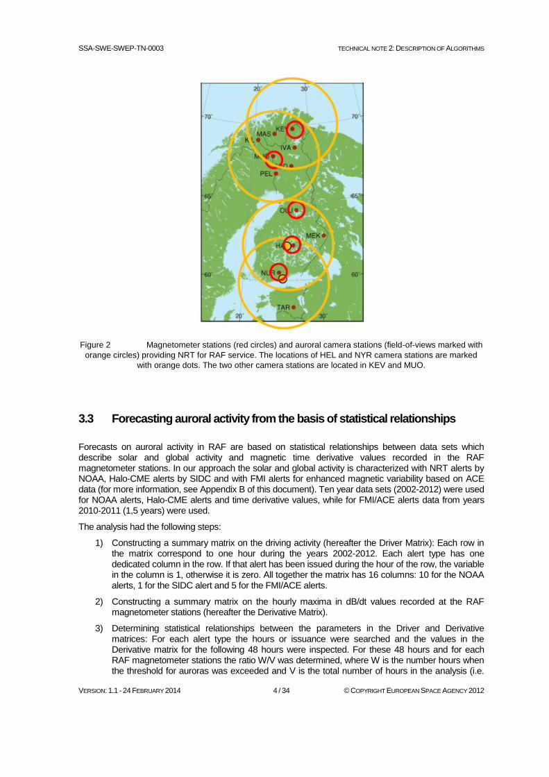
The magnetometer stations which are used in RAF belong to the IMAGE magnetometer chain and are the following NUR (60.50N, 24.65E), HAN (62.25N, 26.60E), OUJ (64.52N, 27.23E), MUO (68.02N, 23.53E) and KEV (69.76N, 27.01E). The stations are located around the same meridian and at latitudes across the southern part of the average auroral zone (c.f. Figure 2). The thresholds used for the stations are 0.30 nT/s (NUR), 0.35 nT/s (HAN), 0.42 nT/s (OUJ), 0.52 nT/s (MUO) and 0.57 nT/s (KEV).
SSA-SWE-SWEP-TN-0003 TECHNICAL NOTE 2: DESCRIPTION OF ALGORITHMS
VERSION: 1.1 - 24 FEBRUARY 2014 4 / 34 © COPYRIGHT EUROPEAN SPACE AGENCY 2012
Figure 2 Magnetometer stations (red circles) and auroral camera stations (field-of-views marked with
orange circles) providing NRT for RAF service. The locations of HEL and NYR camera stations are marked
with orange dots. The two other camera stations are located in KEV and MUO.
3.3 Forecasting auroral activity from the basis of statistical relationships
Forecasts on auroral activity in RAF are based on statistical relationships between data sets which describe solar and global activity and magnetic time derivative values recorded in the RAF magnetometer stations. In our approach the solar and global activity is characterized with NRT alerts by NOAA, Halo-CME alerts by SIDC and with FMI alerts for enhanced magnetic variability based on ACE data (for more information, see Appendix B of this document). Ten year data sets (2002-2012) were used for NOAA alerts, Halo-CME alerts and time derivative values, while for FMI/ACE alerts data from years 2010-2011 (1,5 years) were used.
The analysis had the following steps:
1) Constructing a summary matrix on the driving activity (hereafter the Driver Matrix): Each row in the matrix correspond to one hour during the years 2002-2012. Each alert type has one dedicated column in the row. If that alert has been issued during the hour of the row, the variable in the column is 1, otherwise it is zero. All together the matrix has 16 columns: 10 for the NOAA alerts, 1 for the SIDC alert and 5 for the FMI/ACE alerts.
2) Constructing a summary matrix on the hourly maxima in dB/dt values recorded at the RAF magnetometer stations (hereafter the Derivative Matrix).
3) Determining statistical relationships between the parameters in the Driver and Derivative matrices: For each alert type the hours or issuance were searched and the values in the Derivative matrix for the following 48 hours were inspected. For these 48 hours and for each RAF magnetometer stations the ratio W/V was determined, where W is the number hours when the threshold for auroras was exceeded and V is the total number of hours in the analysis (i.e.

SSA-SWE-SWEP-TN-0003 TECHNICAL NOTE 2: DESCRIPTION OF ALGORITHMS
VERSION: 1.1 - 24 FEBRUARY 2014 5 / 34 © COPYRIGHT EUROPEAN SPACE AGENCY 2012
the number of issuances of the analysed alert type during the ten year period). Figure 3 is an example plot on the probability to record threshold exceeding dB/dt values in KEV during the next 48 hours after the NOAA ALTK06 issuance. According to this plot the opportunity to see auroras with higher than 85% probability is more than 0.5 for 18 hours after the ALTK06 issuance.
4) Identifying those parameters in the Driver matrix which yield W/V values equal or larger than 0.5 or showing otherwise promising behaviour in the above described analysis.
5) Refining the analysis of step 3 by binning the data points according to magnetic local time and by studying the combined effect of some of the most influential driver parameters. Four bins were used in the local time binning: Noon (06-12 UT), midnight (18-24 UT), dawn (00-06 UT) and dusk (12-18 UT). (Note: for the MIRACLE local time sector MLT~UT+2.5h.)
The above described analysis revealed that the following parameters in the Driver Matrix showed potential to become useful input data for the RAF forecast service as they showed W/V values higher than 0.5:
Alerts on enhanced global geomagnetic activity (ALTK04…ALTK09); Binning according to local time yields higher W/V values.
Alerts on enhanced proton fluxes in the geostationary distances (ALTPX1…ALTPX4): If an alert of enhanced proton fluxes (any level from ALTPX1 to ALTPX4) has been issued during 24 hours prior to a ALTK06 the W/V values are higher than in the case of ALTK06 alone. This is taken into account in the forecast service. The thresholds for alerts ALTPX1…ALTPX4 are determined according to the integral flux of protons with energies above 10 MeV. More information is available in the following link: http://www.swpc.noaa.gov/alerts/AlertsTable.html
Alerts on enhanced electron fluxes in the geostationary distances (ALTEF3): Combining with K06-alerts yields higher W/V values (c.f. the case above). The threshold for alert ALTEF3 is determined according to the integral flux of electrons with energies above 2 MeV. More information is available in the following link: http://www.swpc.noaa.gov/alerts/AlertsTable.html
In addition, the following parameters cause a clear enhancement in the probability to record high dB/dt values after some delay, but the enhanced probability does not reach 0.5. These parameters will be used in the Blinking lamps element of the RAF Nowcast page:
X-ray Flare alerts (ALTXMF): Probability for high dB/dt values enhance on average after 37 hours from the alert.
SIDC Halo CME: These alerts have a wide established user community which further motivates their usage in RAF.
FMI/ACE alerts: Probability for high dB/dt values for next 2-3 hours enhanced. The Anow! user community has given positive feedback about the FMI/ACE short time forecasts which encourages their usage also in RAF blinking lights.

SSA-SWE-SWEP-TN-0003 TECHNICAL NOTE 2: DESCRIPTION OF ALGORITHMS
VERSION: 1.1 - 24 FEBRUARY 2014 6 / 34 © COPYRIGHT EUROPEAN SPACE AGENCY 2012
Figure 3 Probability to record dB/dt values higher than 0.57 nT/s in KEV during the 48 hours after the
issuance of NOAA ALTK06 alert.
The reliability of the W/V values given in plots like Figure 3 depends on the number of samples used to derive the curves. For example, in the case of Figure 3 195 samples have been available for each delay time listed in the horizontal axis. The error estimate for the W/V is 1/sqrt(195)~0.07 (assuming that the samples have Poisson distribution).
3.4 Getting information about Cloudiness Cloudiness map is a standard weather prediction model output for Northern Europe. The background model (FMI model HIRLAM or European model ECMWF) is chosen by the forecaster and corrections to the selected model are based on the forecaster's experience. The map has shaded regions for the totally cloudy areas (cloudiness larger than 6/8, i.e. 75% of the sky). The spatial resolution in the maps is 15 km and their time resolution is one hour.
3.5 Getting information about the Sun and Moon rise and set times Rise and set times for the Sun are computed in the RAF code with widely known formulas published in several places in the Internet. The Moon rise and set times and the Moon phases are given in numeric form from a lookup table. The annual lookup tables are created in FMI with the help of tools available in the Internet (see URLs 1 & 2 in Appendix A). The Moon rise and set times are only included during three

SSA-SWE-SWEP-TN-0003 TECHNICAL NOTE 2: DESCRIPTION OF ALGORITHMS
VERSION: 1.1 - 24 FEBRUARY 2014 7 / 34 © COPYRIGHT EUROPEAN SPACE AGENCY 2012
nights before and after the full Moon, when it most disturbs the auroral observations. Full Moon is almost ten times brighter than a half Moon and strongly dilutes the faint colours of the aurora.
3.6 Algorithms
3.6.1 Determining the location of the auroral band based on dB/dt (Nowcast)
Current geomagnetic activity is illustrated in terms of the location of the auroral band on a map where also the locations of the RAF magnetometers stations are shown with dots with varying colors. Maximum time derivative of the horizontal magnetic field component (maximum of max(dX/dt) and max(dY/dt) in nT/s) during one hour is calculated from data recorded at the RAF magnetometer stations. The magnetic data are averaged over one minute from the 10-sec raw data. Once the threshold values are exceeded, the corresponding station location marker on the geographic map changes its colour from black to red. In case of missing data, the station location marker will become an open circle on the map. The dB/dt oval is drawn as a green band to follow the magnetic latitude lines within +- 2 latitude degrees from each station where the derivative threshold is exceeded. From individual station oval bands the northernmost and southernmost boundaries are displayed on the map.
3.6.2 Determining the location of the statistical auroral oval based on Kp
In addition to the dB/dt oval, statistical auroral oval boundaries are plotted on the Fennoscandian map. We use the same approach as presented by Sigernes et al. 2011 ([RD.6]; see URL 3 in Appendix A). From the two options presented by Sigernes et al., the Starkov-oval which is based on ground-based optical data is used in the RAF service. The statistical model uses the global geomagnetic activity index Kp as input parameter. According to this model, the auroral oval boundaries are estimated as polynomials of Kp and as a function of local time. Polynomial coefficients have been calculated for poleward, equatorward and diffuse oval boundaries separately. Kp index is a 3-hour average index ranging from 0 (quiet) to 9 (active). The service of Sigernes et al. uses the one-hour prediction for the planetary Kp index provided by NOAA/SWPC with updating rate of once every 15 min. RAF service will use the Kp proxy provided by NOAA (URL 6 in Appendix A). The geographic position of the statistical auroral oval in the Fennoscandia region depends not only on the Kp value but also on the UT. The RAF service will take into account the UTdependency at least with one-hour time resolution.
3.6.3 The algorithm for OvalMakerNow
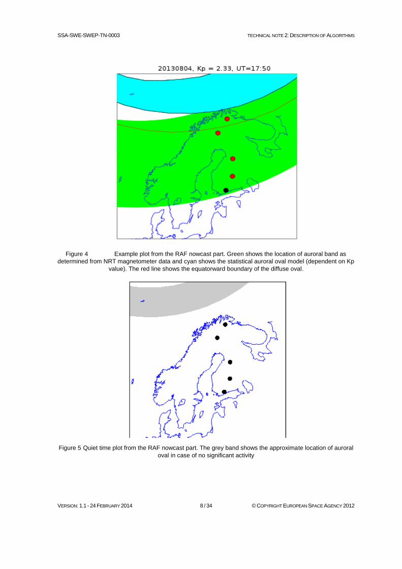
In the two above sections we have described the principles which are used to create the map plots for the RAF nowcasting service. An example of these plots is shown in Figure 4. In this example the discrepancy between the oval derived from NRT dB/dt and that from the model by Sigernes et al. is rather large. In reality the discrepancy will typically smaller. However, there may be situations where the absolute value of magnetic field disturbances are relatively high (i.e. Kp is around 4) but the time derivatives are small (RAF does not show auroras). The opposite may also happen: At the beginning of a storm period high dB/dt values may appear (RAF shows auroras) but Kp values have not yet reached the high levels. In a continuation study we will investigate these controversial situations in order to learn more on the conditions where they appear. Conclusions from this study will be presented in the RAF service introductory pages (How this service works).
SSA-SWE-SWEP-TN-0003 TECHNICAL NOTE 2: DESCRIPTION OF ALGORITHMS
VERSION: 1.1 - 24 FEBRUARY 2014 8 / 34 © COPYRIGHT EUROPEAN SPACE AGENCY 2012
Figure 4 Example plot from the RAF nowcast part. Green shows the location of auroral band as
determined from NRT magnetometer data and cyan shows the statistical auroral oval model (dependent on Kp
value). The red line shows the equatorward boundary of the diffuse oval.
Figure 5 Quiet time plot from the RAF nowcast part. The grey band shows the approximate location of auroral
oval in case of no significant activity
SSA-SWE-SWEP-TN-0003 TECHNICAL NOTE 2: DESCRIPTION OF ALGORITHMS
VERSION: 1.1 - 24 FEBRUARY 2014 9 / 34 © COPYRIGHT EUROPEAN SPACE AGENCY 2012
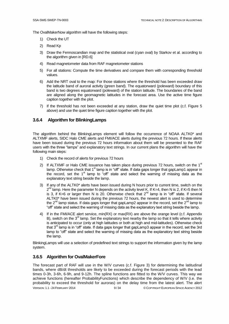
The OvalMakerNow algorithm will have the following steps:
1) Check the UT
2) Read Kp
3) Draw the Fennoscandian map and the statistical oval (cyan oval) by Starkov et al. according to the algorithm given in [RD.6]
4) Read magnetometer data from RAF magnetometer stations
5) For all stations: Compute the time derivatives and compare them with corresponding threshold values.
6) Add the NRT oval to the map: For those stations where the threshold has been exceeded draw the latitude band of auroral activity (green band). The equatorward (poleward) boundary of this band is two degrees equatorward (poleward) of the station latitude. The boundaries of the band are aligned along the geomagnetic latitudes in the forecast area. Use the active time figure caption together with the plot.
7) If the threshold has not been exceeded at any station, draw the quiet time plot (c.f. Figure 5 above) and use the quiet time figure caption together with the plot.
3.6.4 Algorithm for BlinkingLamps
The algorithm behind the BlinkingLamps element will follow the occurrence of NOAA ALTK0* and ALTXMF alerts, SIDC Halo CME alerts and FMI/ACE alerts during the previous 72 hours. If these alerts have been issued during the previous 72 hours information about them will be presented to the RAF users with the three “lamps” and explanatory text strings. In our current plans the algorithm will have the following main steps:
1) Check the record of alerts for previous 72 hours
2) If ALTXMF or Halo CME issuance has taken place during previous 72 hours, switch on the 1st
lamp. Otherwise check that 1st lamp is in “off” state. If data gaps longer that gapLamp1 appear in
the record, set the 1st lamp to “off” state and select the warning of missing data as the
explanatory text string beside the lamp.
3) If any of the ALTK0* alerts have been issued during N hours prior to current time, switch on the 2
nd lamp. Here the parameter N depends on the activity level K. If K=4, then N is 2, if K=5 then N
is 3, if K=6 or larger then N is 20. Otherwise check that 2nd
lamp is in “off” state. If several ALTK0* have been issued during the previous 72 hours, the newest alert is used to determine the 2
nd lamp status. If data gaps longer that gapLamp2 appear in the record, set the 2
nd lamp to
“off” state and select the warning of missing data as the explanatory text string beside the lamp.
4) If in the FMI/ACE alert service, min(RX) or max(RX) are above the orange level (c.f. Appendix B), switch on the 3
rd lamp. Set the explanatory text nearby the lamp so that it tells where activity
is anticipated to occur (only at high latitudes or both at high and mid-latitudes). Otherwise check that 3
rd lamp is in “off” state. If data gaps longer that gapLamp3 appear in the record, set the 3rd
lamp to “off” state and select the warning of missing data as the explanatory text string beside the lamp.
BlinkingLamps will use a selection of predefined text strings to support the information given by the lamp system.
3.6.5 Algorithm for OvalMakerFore
The forecast part of RAF will use in the W/V curves (c.f. Figure 3) for determining the latitudinal bands, where dB/dt thresholds are likely to be exceeded during the forecast periods with the lead times 0-3h, 3-6h, 6-9h, and 9-12h. The spline functions are fitted to the W/V curves. This way we achieve functions (hereafter ProbabilityFunctions) which describe the dependency of W/V (i.e. the probability to exceed the threshold for auroras) on the delay time from the latest alert. The alert
SSA-SWE-SWEP-TN-0003 TECHNICAL NOTE 2: DESCRIPTION OF ALGORITHMS
VERSION: 1.1 - 24 FEBRUARY 2014 10 / 34 © COPYRIGHT EUROPEAN SPACE AGENCY 2012
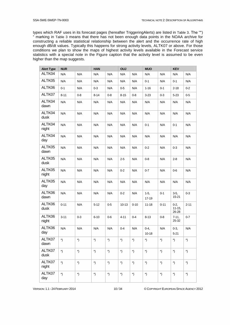
types which RAF uses in its forecast pages (hereafter TriggeringAlerts) are listed in Table 3. The “*) “ marking in Table 3 means that there has not been enough data points in the NOAA archive for constructing a reliable statistical relationship between the alert and the occurrence rate of high enough dB/dt values. Typically this happens for strong activity levels, ALTK07 or above. For those conditions we plan to show the maps of highest activity levels available in the Forecast service statistics with a special note in the Figure caption that the activity level is assumed to be even higher than the map suggests.
Alert Type NUR HAN OUJ MUO KEV
ALTK04 N/A N/A N/A N/A N/A N/A N/A N/A N/A N/A
ALTK05 N/A N/A N/A N/A N/A N/A 0-1 N/A 0-1 N/A
ALTK06 0-1 N/A 0-3 N/A 0-5 N/A 1-16 0-1 2-18 0-2
ALTK07 8-11 0-8 8-14 0-8 8-15 0-8 3-23 0-3 5-23 0-5
ALTK04 dawn
N/A N/A N/A N/A N/A N/A N/A N/A N/A N/A
ALTK04 dusk
N/A N/A N/A N/A N/A N/A N/A N/A N/A N/A
ALTK04 night
N/A N/A N/A N/A N/A N/A 0-1 N/A 0-1 N/A
ALTK04 day
N/A N/A N/A N/A N/A N/A N/A N/A N/A N/A
ALTK05 dawn
N/A N/A N/A N/A N/A N/A 0-2 N/A 0-3 N/A
ALTK05 dusk
N/A N/A N/A N/A 2-5 N/A 0-8 N/A 2-8 N/A
ALTK05 night
N/A N/A N/A N/A 0-2 N/A 0-7 N/A 0-6 N/A
ALTK05 day
N/A N/A N/A N/A N/A N/A N/A N/A N/A N/A
ALTK06 dawn
N/A N/A N/A N/A 0-2 N/A 1-5,
17-19
0-1 3-5, 15-21
0-3
ALTK06 dusk
0-11 N/A 5-12 0-5 10-13 0-10 11-18 0-11 0-2, 11-15, 26-28
2-11
ALTK06 night
3-11 0-3 6-10 0-6 4-11 0-4 8-13 0-8 7-11, 25-32
0-7
ALTK06 day
N/A N/A N/A N/A 0-4 N/A 0-4,
10-18
N/A 0-3,
5-21
N/A
ALTK07 dawn
*) *) *) *) *) *) *) *) *) *)
ALTK07 dusk
*) *) *) *) *) *) *) *) *) *)
ALTK07 night
*) *) *) *) *) *) *) *) *) *)
ALTK07 day
*) *) *) *) *) *) *) *) *) *)
SSA-SWE-SWEP-TN-0003 TECHNICAL NOTE 2: DESCRIPTION OF ALGORITHMS
VERSION: 1.1 - 24 FEBRUARY 2014 11 / 34 © COPYRIGHT EUROPEAN SPACE AGENCY 2012
Alert Type NUR HAN OUJ MUO KEV
ALTK04
& EF3
N/A N/A N/A N/A N/A N/A N/A N/A N/A N/A
ALTK04
& PX
N/A N/A N/A N/A N/A N/A N/A N/A N/A N/A
ALTK05
& EF3
N/A N/A N/A N/A N/A N/A 0-2 N/A 0-3 N/A
ALTK05
& PX
N/A N/A N/A N/A 0-1 N/A 0-5 N/A 1-5 0-1
ALTK06
& EF3
0-3 N/A 0-3 N/A 1-4 0-1 1-12 0-1 3-18 0-3
ALTK06
& PX
3-13 0-3 5-13 0-5 4-13 0-4 5-30 0-5 12-24 0-12
ALTK07
& EF3
9-13 0-9 10-15 0-10 5-12 0-5 0-12 N/A 6-18 0-6
ALTK07
& PX
10-16 0-10 10-18 0-10 9-20 0-9 20-25 0-20 20-48 0-20
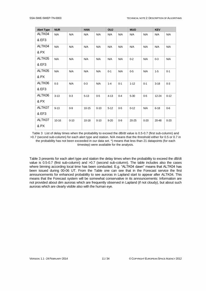
Table 3 List of delay times when the probability to exceed the dB/dt value is 0.5-0.7 (first sub-column) and
>0.7 (second sub-column) for each alert type and station. N/A means that the threshold either for 0.5 or 0.7 in
the probability has not been exceeded in our data set. *) means that less than 21 datapoints (for each
timestep) were available for the analysis.
Table 3 presents for each alert type and station the delay times when the probability to exceed the dB/dt value is 0.5-0.7 (first sub-column) and >0.7 (second sub-column). The table includes also the cases where binning according local time has been conducted. E.g. “ALTK04 dawn” means that ALTK04 has been issued during 00-06 UT. From the Table one can see that in the Forecast service the first announcements for enhanced probability to see auroras in Lapland start to appear after ALTK04. This means that the Forecast system will be somewhat conservative in its announcements: Information are not provided about dim auroras which are frequently observed in Lapland (if not cloudy), but about such auroras which are clearly visible also with the human eye.
SSA-SWE-SWEP-TN-0003 TECHNICAL NOTE 2: DESCRIPTION OF ALGORITHMS
VERSION: 1.1 - 24 FEBRUARY 2014 12 / 34 © COPYRIGHT EUROPEAN SPACE AGENCY 2012
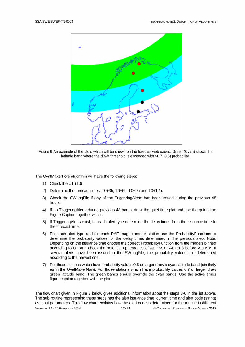
Figure 6 An example of the plots which will be shown on the forecast web pages. Green (Cyan) shows the
latitude band where the dB/dt threshold is exceeded with >0.7 (0.5) probability.
The OvalMakerFore algorithm will have the following steps:
1) Check the UT (T0)
2) Determine the forecast times, T0+3h, T0+6h, T0+9h and T0+12h.
3) Check the SWLogFile if any of the TriggeringAlerts has been issued during the previous 48 hours.
4) If no TriggeringAlerts during previous 48 hours, draw the quiet time plot and use the quiet time Figure Caption together with it.
5) If TriggeringAlerts exist, for each alert type determine the delay times from the issuance time to the forecast time.
6) For each alert type and for each RAF magnetometer station use the ProbabilityFunctions to determine the probability values for the delay times determined in the previous step. Note: Depending on the issuance time choose the correct ProbabilityFunction from the models binned according to UT and check the potential appearance of ALTPX or ALTEF3 before ALTK0*. If several alerts have been issued in the SWLogFile, the probability values are determined according to the newest one.
7) For those stations which have probability values 0.5 or larger draw a cyan latitude band (similarly as in the OvalMakerNow). For those stations which have probability values 0.7 or larger draw green latitude band. The green bands should override the cyan bands. Use the active times figure caption together with the plot.
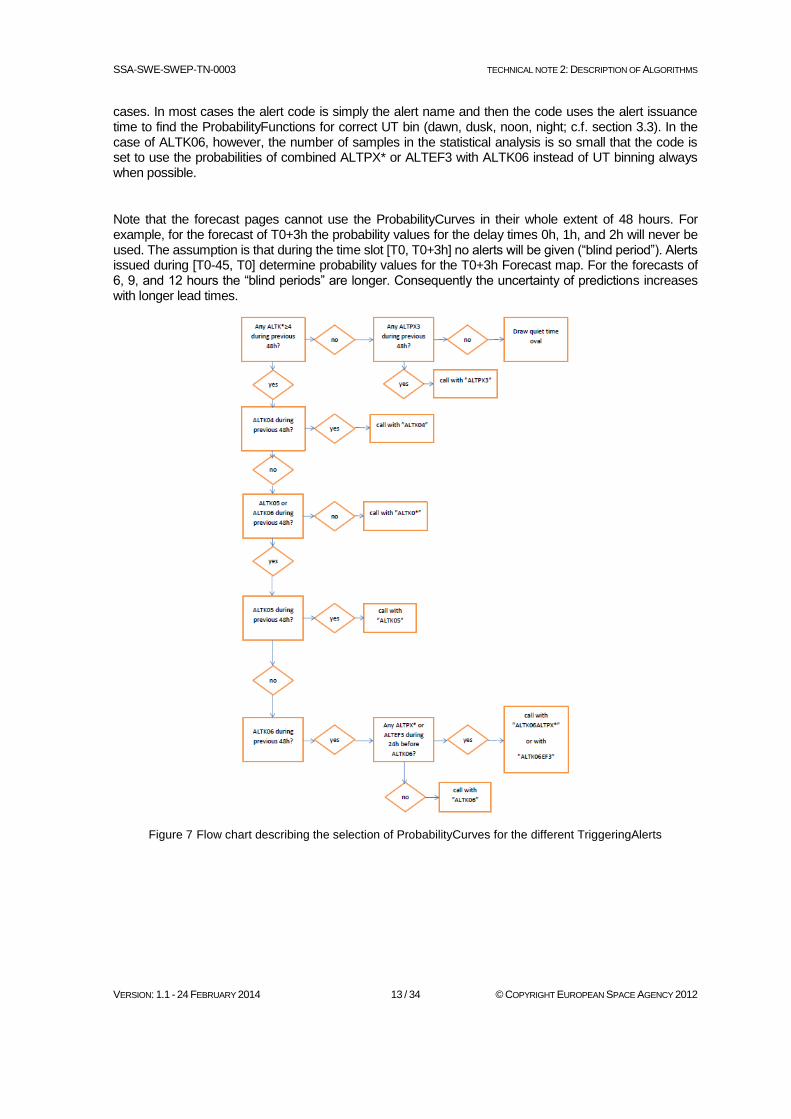
The flow chart given in Figure 7 below gives additional information about the steps 3-6 in the list above. The sub-routine representing these steps has the alert issuance time, current time and alert code (string) as input parameters. This flow chart explains how the alert code is determined for the routine in different
SSA-SWE-SWEP-TN-0003 TECHNICAL NOTE 2: DESCRIPTION OF ALGORITHMS
VERSION: 1.1 - 24 FEBRUARY 2014 13 / 34 © COPYRIGHT EUROPEAN SPACE AGENCY 2012
cases. In most cases the alert code is simply the alert name and then the code uses the alert issuance time to find the ProbabilityFunctions for correct UT bin (dawn, dusk, noon, night; c.f. section 3.3). In the case of ALTK06, however, the number of samples in the statistical analysis is so small that the code is set to use the probabilities of combined ALTPX* or ALTEF3 with ALTK06 instead of UT binning always when possible.
Note that the forecast pages cannot use the ProbabilityCurves in their whole extent of 48 hours. For example, for the forecast of T0+3h the probability values for the delay times 0h, 1h, and 2h will never be used. The assumption is that during the time slot [T0, T0+3h] no alerts will be given (“blind period”). Alerts issued during [T0-45, T0] determine probability values for the T0+3h Forecast map. For the forecasts of 6, 9, and 12 hours the “blind periods” are longer. Consequently the uncertainty of predictions increases with longer lead times.
Figure 7 Flow chart describing the selection of ProbabilityCurves for the different TriggeringAlerts
SSA-SWE-SWEP-TN-0003 TECHNICAL NOTE 2: DESCRIPTION OF ALGORITHMS
VERSION: 1.1 - 24 FEBRUARY 2014 14 / 34 © COPYRIGHT EUROPEAN SPACE AGENCY 2012
4. The Ionospheric Scintillation Monitoring
4.1 Ionosphere observation with GPS
The ionosphere acts as a dispersive medium on the GPS radio signal. It applies a group delay and a phase advance respectively to the code and carrier observables. Combining the two GPS frequencies is useful to isolate this effect and obtain some information on the ionosphere
4.1.1 Pseudo-range or code observation
The C/A-, P-, or Y-code k
iP , transmitted by satellite k at time tk and registered by receiver i at time ti is
defined as (Schaer, 1999; [RD.8]):
)()()( ,, i
kk
ionoi
k
tropi
k
i
k
i
k
i
k
i bbcttcttcP
where
k
i is the geometric distance between the satellite and the receiver
k
i tt , are the receiver and satellite clocks offsets with respect to the GPS system time,
k
tropi, is the tropospheric delay,
k
ioni, is the ionospheric delay,
i
k bb , are the satellite and receiver hardware delays, expressed in unit of time,
is a random error (or residual).
k
iP estimated uncertainties are 3 meters for C/A code and 0.3 m for P-code.
4.1.2 Carrier phase observation
The carrier phase observation is nearly the same with:
k
i
k
ionoi
k
tropi
k
i
k
i
k
i BttcL ,,)(
where:
is the corresponding wavelength and
k
iB is the constant bias (initial carrier phase ambiguity k
iN ), expressed in cycles
Estimated uncertainties ofk
iL is 2 mm.
For dual-frequency geodetic GPS receivers, a simplified frequency-dependent notation (1=1575.42
MHz, 2=1227.60 MHz) is adopted k
tropi
k
i
k
i
k
i ttc ,
' )(
P-code observations on both frequencies can be written as:
SSA-SWE-SWEP-TN-0003 TECHNICAL NOTE 2: DESCRIPTION OF ALGORITHMS
VERSION: 1.1 - 24 FEBRUARY 2014 15 / 34 © COPYRIGHT EUROPEAN SPACE AGENCY 2012
)(' 1,
1,
1, i
kk
iono
k
i
k
i bbcP
)(' 2,
2,
2, i
kk
iono
k
i
k
i bbcP
Carrier phase observations on both frequencies can be written as:
k
i
k
iono
k
i
k
i BL 1,1, '
k
i
k
iono
k
i
k
i BL 2,2, '
where 647.1/ 2
2
2
1 . To keep equations simple the term has been omitted.
4.1.3 Geometry-free linear combination
The linear combination 214 LLL , resp. 214 PPP , is simply obtained by subtracting the second
frequency from the first on carrier phase, resp. code. The assumption is done that receivers track the satellite simultaneously with both frequencies. This LC is also called the Geometry-free linear
combination because it eliminates the geometric term' .
The LC leads to undifferenced observation equations:
k
i
k
iono
k
i BL 4,44,
)(44, i
kk
iono
k
i bbcP (LC G-F)
where 647.0/11 2
2
2
14 and k
iB 4, is an ambiguity parameter.
From these formulas, the determination of the absolute ionospheric delay suffers from the unknown
parameters: the differential code biases (DCBs) ckb and c ib for satellite and receivers as well as
the ambiguity parameterk
iB 4, .
4.1.4 TEC computation
Across the ionosphere, the signals are both bent and retarded because of the electronic density of the medium. The ionospheric path delay results from the integration of the refractive index as follows:
2
2)( TEC
Cdn x
iono where
233.402
smCx
(>0 for code and <0 for phase),
TEC is the line-of-sight or slant Total Electronic Content in 1016
electrons per square meter (TECU unit),
and is the frequency.
The ionospheric path delay is about 0.162m/TECU at frequency 1.
SSA-SWE-SWEP-TN-0003 TECHNICAL NOTE 2: DESCRIPTION OF ALGORITHMS
VERSION: 1.1 - 24 FEBRUARY 2014 16 / 34 © COPYRIGHT EUROPEAN SPACE AGENCY 2012
4.2 Algorithms for key parameters calculation
4.2.1 ROTI
The Rate of TEC Index (ROTI) is an indicator of ionospheric phase scintillations applicable with geodetic 1 Hz or 1/30 Hz GPS receivers. The ROTI is the standard deviation of the time derivative of the ionospheric delay, deduced from the carrier.
To monitor the time variation of the TEC one can calculate the geometry free linear combination LC6 of
successive observations at time lt and time 1lt with the same receiver i. LC6 expression for phase is
then:
))()((2
)()( 1
2
1416
l
k
il
k
ix
l
k
il
k
i
k
i tTECtTECC
tLtLL (LC temp)
The slant TEC variation in time )()( 1 l
k
il
k
i
k
i tTECtTECTEC can be derived as long as no cycle
slip occurs.
The ROTI is then expressed as:
)( k
iTECROTI
4.2.2 IndexDtDS1
The IndexDtDS1 is an indicator of amplitude scintillations obtained from geodetic GPS receivers. It corresponds to the standard deviation of the time derivative of S1 (signal amplitude on L1).
)(1 1,
k
iSIndexDtDS
The following table shows the period used for the statistics of the two indices:
Observation rate Number of observations Period
1 Hz 60 1 min
1/30 Hz 10 5 min
Table 4 Indices and periods
4.2.3 Single layer model
To convert the GPS observations into ionospheric data, a common model is to consider the ionosphere as a thin shell localized at an altitude of 400 km above the WGS-84 ellipsoid, which corresponds approximately to the ionization maximum of the real ionosphere.
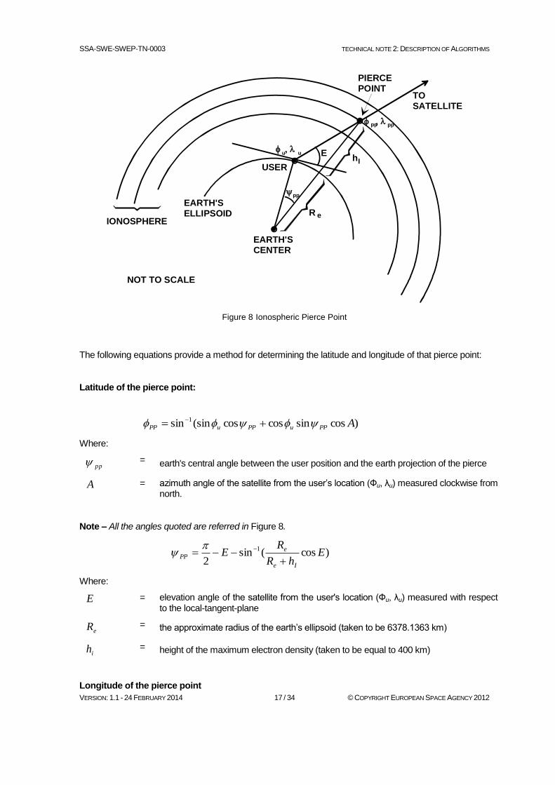
4.2.3.1 Ionospheric Pierce Points
The intersection of the satellite – receiver line of sight with the shell is called the Ionospheric Pierce Point
(IPP), represented in Figure 8. Its location is defined in WGS-84 latitude (pp) and longitude (λpp).
SSA-SWE-SWEP-TN-0003 TECHNICAL NOTE 2: DESCRIPTION OF ALGORITHMS
VERSION: 1.1 - 24 FEBRUARY 2014 17 / 34 © COPYRIGHT EUROPEAN SPACE AGENCY 2012
E
pp
u u
pp pp
EARTH'SCENTER
EARTH'SELLIPSOID
IONOSPHERE
hI
R e
USER
TOSATELLITE
PIERCEPOINT
NOT TO SCALE
Figure 8 Ionospheric Pierce Point
The following equations provide a method for determining the latitude and longitude of that pierce point:
Latitude of the pierce point:
)cossincoscos(sinsin 1 APPuPPuPP
Where:
pp = earth's central angle between the user position and the earth projection of the pierce
A = azimuth angle of the satellite from the user’s location (Фu, λu) measured clockwise from north.
Note – All the angles quoted are referred in Figure 8.
)cos(sin2
1 EhR
RE
Ie
ePP
Where:
E = elevation angle of the satellite from the user's location (Фu, λu) measured with respect to the local-tangent-plane
eR
= the approximate radius of the earth’s ellipsoid (taken to be 6378.1363 km)
ih
= height of the maximum electron density (taken to be equal to 400 km)
Longitude of the pierce point

SSA-SWE-SWEP-TN-0003 TECHNICAL NOTE 2: DESCRIPTION OF ALGORITHMS
VERSION: 1.1 - 24 FEBRUARY 2014 18 / 34 © COPYRIGHT EUROPEAN SPACE AGENCY 2012
PP
PPu
PP
PPu
PP
A
A
cos
sinsinsin
cos
sinsinsin
1
1
otherwise
2tancostan and 70
ifor 2
tancostan and 70 if
uPPu
uPPu
AA
A
4.2.3.2 Slant TEC to Vertical TEC
The electronic content measured along the slant path of the signal depends on the angle at which it crosses the ionosphere and needs to be projected into the vertical TEC. The relation between the vertical VTEC or TEC(0) and the slant TEC(z) if z and the satellite zenith distance at the receiver’s location is:
'2zs in-1
1 TEC(0) TEC(z) with
H R
R z s in
'sin z
z’ being the satellite’s zenith distance at the point where the single layer is pierced.
The different angles and distances are defined in Figure 9.
Figure 9 Single layer model
4.2.4 TEC Calibration
The TEC derived from the geometry-free linear combination still contains the satellite and receivers differential clock biases (DCBs) that need to be removed to obtain the absolute value.
The satellite biases are computed each day and published by the IGS Analysis Centers. The ISM routines directly use the ones computed by the Center for Orbit Determination in Europe (CODE).
SSA-SWE-SWEP-TN-0003 TECHNICAL NOTE 2: DESCRIPTION OF ALGORITHMS
VERSION: 1.1 - 24 FEBRUARY 2014 19 / 34 © COPYRIGHT EUROPEAN SPACE AGENCY 2012
Receiver biases are also published, but for a limited set of IGS stations, that does not cover the whole network used for the ISM service. The method used to determine them independently is adapted from (Ma & Maruyama, 2003; [RD.7]).
If the vertical TEC is calculated from a slant TEC still containing the receiver clock bias, for one satellite at an elevation z:
F(z) . TEC(0) DCB TEC(z) ,
where
TEC(z) is the unbiased slant TEC
DCB is the receiver differential clock bias
TEC(0) is the vertical TEC
F(z) is the projection function
The principle of the method is to assume that the ionosphere is homogeneous between all the satellites in sight of the receiver at a given time. Then, the correct DCB will minimize the differences between the vertical TEC obtained from all the satellites.

SSA-SWE-SWEP-TN-0003 TECHNICAL NOTE 2: DESCRIPTION OF ALGORITHMS
VERSION: 1.1 - 24 FEBRUARY 2014 20 / 34 © COPYRIGHT EUROPEAN SPACE AGENCY 2012
5. Ionospheric Scintillation Mapping
5.1 Introduction
As a result of propagation through ionosphere electron density irregularities, transionospheric radio signals may experience amplitude and phase fluctuations. In equatorial regions, these signal fluctuations specially occur during equinoxes, after sunset, and last for a few hours. They are more intense in periods of high solar activity. There is also a longitudinal dependency. Scintillations are more common in South America near the December solstice than at the equinoxes. These fluctuations result in signal degradation from VHF up to C band. They are a major issue for many systems including Global Navigation Satellite Systems (GNSS), telecommunications, remote sensing and earth observation systems.
The signal fluctuations, referred as scintillations, are created by random fluctuations of the medium’s refractive index, which are caused by inhomogeneities inside the ionosphere. These inhomogeneities are sub structures of bubbles, which may reach dimensions of several hundreds of kilometers as can be seen from radar observations (Costa et al, 2011; [RD.15]). These bubbles present a patchy structure. They appear after sunset, when the sun ionization drops to zero. Instability processes develop inside these bubbles with creation of turbulences inside the medium. As a result, depletions of electron density appear. In the L band and for the distances usually considered, the diffracting pattern of inhomogeneities in the range of one kilometer size, is inside the first Fresnel zone and contribute to scintillation.
The aim of this work is the development of an algorithm for scintillation mapping for both nowcast and forecast purposes. This mapping will address regional areas at any location on earth and will use as much as possible real time measured data.
Section 5.2 of this chapter presents the results of a raw data analysis and in particular the effects of undersampling as most of the available data do not meet the sampling requirements.
Section Fehler! Verweisquelle konnte nicht gefunden werden. presents the modeling algorithm which will be used as a replacement in case of lack of data.
Section 5.4 is a list of the available sources which could be used for this work.
Section Fehler! Verweisquelle konnte nicht gefunden werden. presents the scintillation mapping algorithm.
Section 5.6 presents some preliminary results.
5.2 Raw data analysis
5.2.1 Introduction
The considered raw data were recorded in Cayenne (French Guiana) in the frame of the PRIS measurement campaign (Béniguel, 2009; [RD.11]). The days 314 to 318 in year 2006 are taken into
SSA-SWE-SWEP-TN-0003 TECHNICAL NOTE 2: DESCRIPTION OF ALGORITHMS
VERSION: 1.1 - 24 FEBRUARY 2014 21 / 34 © COPYRIGHT EUROPEAN SPACE AGENCY 2012
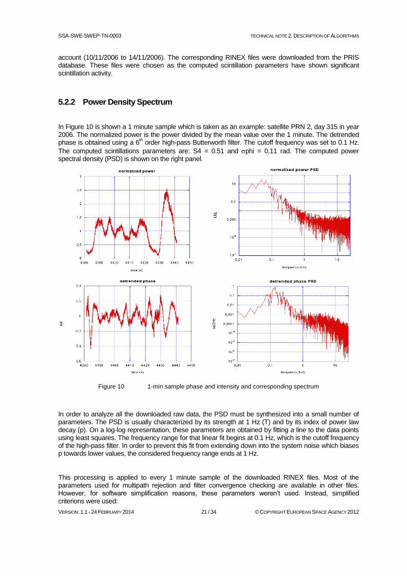
account (10/11/2006 to 14/11/2006). The corresponding RINEX files were downloaded from the PRIS database. These files were chosen as the computed scintillation parameters have shown significant scintillation activity.
5.2.2 Power Density Spectrum
In Figure 10 is shown a 1 minute sample which is taken as an example: satellite PRN 2, day 315 in year 2006. The normalized power is the power divided by the mean value over the 1 minute. The detrended phase is obtained using a 6
th order high-pass Butterworth filter. The cutoff frequency was set to 0.1 Hz.
The computed scintillations parameters are: S4 = 0.51 and phi = 0.11 rad. The computed power spectral density (PSD) is shown on the right panel.
Figure 10 1-min sample phase and intensity and corresponding spectrum
In order to analyze all the downloaded raw data, the PSD must be synthesized into a small number of parameters. The PSD is usually characterized by its strength at 1 Hz (T) and by its index of power law decay (p). On a log-log representation, these parameters are obtained by fitting a line to the data points using least squares. The frequency range for that linear fit begins at 0.1 Hz, which is the cutoff frequency of the high-pass filter. In order to prevent this fit from extending down into the system noise which biases p towards lower values, the considered frequency range ends at 1 Hz.
This processing is applied to every 1 minute sample of the downloaded RINEX files. Most of the parameters used for multipath rejection and filter convergence checking are available in other files. However, for software simplification reasons, these parameters weren’t used. Instead, simplified criterions were used:

SSA-SWE-SWEP-TN-0003 TECHNICAL NOTE 2: DESCRIPTION OF ALGORITHMS
VERSION: 1.1 - 24 FEBRUARY 2014 22 / 34 © COPYRIGHT EUROPEAN SPACE AGENCY 2012
No missing measurements (3000 points in a 1 minute sample)
S4 > 0.2 to avoid weak multipath
phi < 2. to check the filter convergence
The histograms of the p index for the power and of the detrended phase PSD are shown in Figure 11. These histograms are directly related to the probability density distributions of p. It can be observed that both distributions are centered on 2.8. Usually, p is considered to be in the range between 1 and 4.
Figure 11 p slope spectrum histograms of intensity and phase scintillation
The phase PSD can be approximated by Tf-p. As a consequence, the phase standard deviation phi is
expressed as following, where fc is the cutoff frequency:
1) p (if )1(
2
122)(2
1
12
p
fc
p
fc
p
fcfcp
T
p
fTdfTfdffPSDphi
5.2.3 Under sampling effects
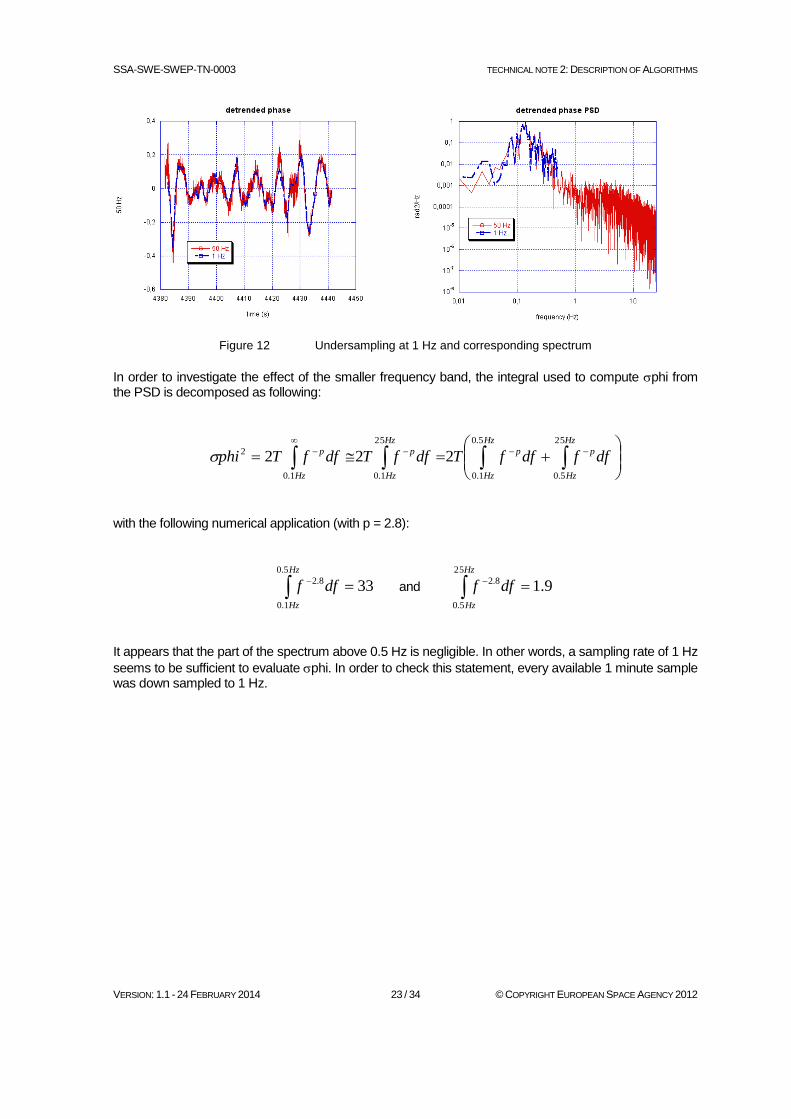
Figure 12 presents the effect of an under sampling for the previous example (satellite PRN 2, day 315 in year 2006). The detrended 50 Hz raw data were sampled down to 1 Hz. As a consequence, the explored frequency range drops from 25 Hz to 0.5 Hz. As in the IGS data processing only the phase is taken into account, in this part only the phase is considered. In this example, it appears that the effect of the 1 Hz sampling is moderate.
SSA-SWE-SWEP-TN-0003 TECHNICAL NOTE 2: DESCRIPTION OF ALGORITHMS
VERSION: 1.1 - 24 FEBRUARY 2014 23 / 34 © COPYRIGHT EUROPEAN SPACE AGENCY 2012
Figure 12 Undersampling at 1 Hz and corresponding spectrum
In order to investigate the effect of the smaller frequency band, the integral used to compute phi from the PSD is decomposed as following:
Hz
Hz
Hz
Hz
pp
Hz
Hz
p
Hz
p dffdffTdffTdffTphi
5.0
1.0
25
5.0
25
1.01.0
2 222
with the following numerical application (with p = 2.8):
33
5.0
1.0
8.2
Hz
Hz
dff and 9.1
25
5.0
8.2
Hz
Hz
dff
It appears that the part of the spectrum above 0.5 Hz is negligible. In other words, a sampling rate of 1 Hz
seems to be sufficient to evaluate phi. In order to check this statement, every available 1 minute sample was down sampled to 1 Hz.

SSA-SWE-SWEP-TN-0003 TECHNICAL NOTE 2: DESCRIPTION OF ALGORITHMS
VERSION: 1.1 - 24 FEBRUARY 2014 24 / 34 © COPYRIGHT EUROPEAN SPACE AGENCY 2012
The phi computed over these 60 points samples are compared with the phi computed over the full 3000 points samples. The results of this comparison are presented in Figure 13. It is noticed that the 1
Hz phi is a good estimation of the 50 Hz phi.
Figure 13 Phase index calculation using 50 Hz data as compared to a 1 Hz data calculation
The effects of a 0.03 Hz (30 s) sampling rate is more difficult to study as this frequency is below the cutoff frequency of the high-pass filter.
5.2.4 S4 comparison over one night of observation
This undersampling study has been complemented by a 1 Hz IGS data analysis from Kourou, located at a short distance from Cayenne. The chosen index for IGS data is the ROTI index (Valette et al., 2007; [RD.18]). This phase index is deducted from the change rate in geometry after removing mean variation using L1 and L2 frequencies. A day of intense scintillations at Cayenne was selected for this comparison. Figure 14 shows the comparison between the 1-min S4 index recorded by the GSVreceiver in Cayenne, and the empirical ROTI scintillation index derived from the IGS 1 s data in Kourou. As can be seen, the major trends can be observed. This enables, through IGS high rate network use, to get some information on the scintillation activity.

SSA-SWE-SWEP-TN-0003 TECHNICAL NOTE 2: DESCRIPTION OF ALGORITHMS
VERSION: 1.1 - 24 FEBRUARY 2014 25 / 34 © COPYRIGHT EUROPEAN SPACE AGENCY 2012
Figure 14 S4 index and ROTI index calculated from 50 Hz and 1 Hz data at two close locations
5.3 GISM Modelling
5.3.1 Introduction
The Global Ionospheric Scintillation Propagation Model (GISM) uses the Multiple Phase Screen technique (MPS) (Knepp, 1983 [RD.12], Béniguel, 2002 [RD.9] & 2004 [RD.10], Gherm, 2005 [RD.16]). The locations of transmitter and receiver are arbitrary. The incidence link angle is arbitrary regarding the ionosphere layers and to the magnetic field vector orientation. It can cross the entire ionosphere or a small part of it. At each screen location along the line of sight, the parabolic equation (PE) is solved. GISM allows calculating mean errors and scintillations due to propagation through the ionosphere.
The mean errors are obtained using a ray technique solving the Haselgrove equations (Budden, 1985; [RD.14]). The ionosphere electronic density at any point inside the medium, required for this calculation, is provided by the NeQuick model (Radicella, 2009; [RD.17]), which is included in the GISM.
The line of sight being determined, the fluctuations are calculated in a second stage using the multiple phase screen technique. The medium is divided into successive layers, each of them acting as a phase screen and the field is scattered from one screen to the next one.
Inputs of the model are the transmitter and receiver locations, the time, day and year of observation, and the geophysical parameters. Based on the PRIS measurements campaign, experimental laws have been derived for the geographic and local time dependency. The spectrum of inhomogeneities is linear in

SSA-SWE-SWEP-TN-0003 TECHNICAL NOTE 2: DESCRIPTION OF ALGORITHMS
VERSION: 1.1 - 24 FEBRUARY 2014 26 / 34 © COPYRIGHT EUROPEAN SPACE AGENCY 2012
a Log – Log scale representation. It is characterized by three parameters: the slope, a typical dimension
of inhomogeneities and the strength. Default values are respectively set to p = 3, 0L = 1 kilometre
and N 0.1 eNe . As geophysical input parameters, only the average 10.7 cm solar flux number is
considered. Its value is taken from the curves published by the National Oceanic and Atmospheric Administration (www.noaa.gov). The magnetic activity is ignored. It is not considered either in the NeQuick model.
GISM calculates a mean value of the scintillation indices both for intensity and phase fluctuations. More details can be found in (Béniguel, 2011; [RD.13]).
5.3.2 Comparison with measurements
The results reported hereafter are taken from the PRIS measurement campaign (Béniguel, 2009; [RD.11]) carried out under ESA / ESTEC contract N° 19530. For this study, a number of receivers were deployed both at low and high latitudes, in particular in Vietnam, Indonesia, Guiana, Cameroon, Chad and Sweden. These receivers were dedicated receivers, operating at 50 Hz. A data bank was constituted and the scintillation characteristics were derived from an extensive analysis of this data bank. Comparisons between measurements and results provided by the GISM model in the same conditions (re playing the scenarios) were performed both for the scintillation indices and on the spectrum.
Scintillation indices
One week of measurements at Cayenne, French Guiana was selected. The results are presented in Figure 15. The x axis corresponds to local time at receiver location. The 0 value has been set arbitrarily to Saturday 19:00, the week of observation.
0
0.2
0.4
0.6
0.8
1
-40 -20 0 20 40 60 80 100
S4 all satellites
Cayenne days 314 to 319 : year 2006
PRN2
PRN13
PRN10
PRN4
PRN24
PRN28
PRN17
PRN12
PRN8
PRN29
PRN26
PRN9
PRN6
PRN23
S4
LT
0
0.2
0.4
0.6
0.8
1
-40 -20 0 20 40 60 80 100
Sigma Phi all satellites
Cayenne, days 314 to 319 / year 2006
PRN2
PRN13
PRN10
PRN4
PRN24
PRN28
PRN17
PRN12
PRN8
PRN29
PRN26
PRN9
PRN6
PRN23
Sig
ma
Ph
i (r
ad
ian
)
LT
Figure 15 Intensity and phase scintillation indices measurements on GPS week N° 377
The local time of the x axis corresponds to hours in GPS time. Each point corresponds to a 1 minute sample. Only points with a S4 value greater than 0.2 were retained in the analysis. A 5° mask elevation angle was taken when recording the data. In addition multipath is rejected using the code carrier divergence algorithm recommended in the Novatel GSV 4004 user manual. As can be seen in the Figure, the points are clustered every evening at post sunset hours, typically 19:00 - 24:00. No average is taken on the data. The scintillation activity occurred quite regularly that week with comparable levels. The S4 average value is about 0.4. The flux number that week (GPS week N° 377, modulo 1024) was equal to 90.
SSA-SWE-SWEP-TN-0003 TECHNICAL NOTE 2: DESCRIPTION OF ALGORITHMS
VERSION: 1.1 - 24 FEBRUARY 2014 27 / 34 © COPYRIGHT EUROPEAN SPACE AGENCY 2012
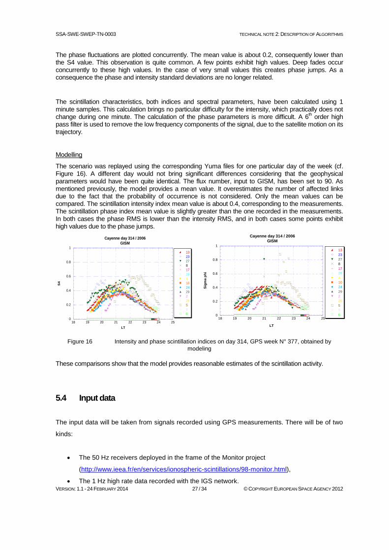
The phase fluctuations are plotted concurrently. The mean value is about 0.2, consequently lower than the S4 value. This observation is quite common. A few points exhibit high values. Deep fades occur concurrently to these high values. In the case of very small values this creates phase jumps. As a consequence the phase and intensity standard deviations are no longer related.
The scintillation characteristics, both indices and spectral parameters, have been calculated using 1 minute samples. This calculation brings no particular difficulty for the intensity, which practically does not change during one minute. The calculation of the phase parameters is more difficult. A 6
th order high
pass filter is used to remove the low frequency components of the signal, due to the satellite motion on its trajectory.
Modelling
The scenario was replayed using the corresponding Yuma files for one particular day of the week (cf. Figure 16). A different day would not bring significant differences considering that the geophysical parameters would have been quite identical. The flux number, input to GISM, has been set to 90. As mentioned previously, the model provides a mean value. It overestimates the number of affected links due to the fact that the probability of occurrence is not considered. Only the mean values can be compared. The scintillation intensity index mean value is about 0.4, corresponding to the measurements. The scintillation phase index mean value is slightly greater than the one recorded in the measurements. In both cases the phase RMS is lower than the intensity RMS, and in both cases some points exhibit high values due to the phase jumps.
0
0.2
0.4
0.6
0.8
1
18 19 20 21 22 23 24 25
Cayenne day 314 / 2006
GISM
13
23
27
8
17
28
4
10
24
29
2
26
5
9
6
S4
LT
0
0.2
0.4
0.6
0.8
1
18 19 20 21 22 23 24 25
Cayenne day 314 / 2006
GISM
13
23
27
8
17
28
4
10
24
29
2
26
5
9
6
Sig
ma
ph
i
LT
Figure 16 Intensity and phase scintillation indices on day 314, GPS week N° 377, obtained by
modeling
These comparisons show that the model provides reasonable estimates of the scintillation activity.
5.4 Input data
The input data will be taken from signals recorded using GPS measurements. There will be of two
kinds:
The 50 Hz receivers deployed in the frame of the Monitor project
(http://www.ieea.fr/en/services/ionospheric-scintillations/98-monitor.html),
The 1 Hz high rate data recorded with the IGS network.
SSA-SWE-SWEP-TN-0003 TECHNICAL NOTE 2: DESCRIPTION OF ALGORITHMS
VERSION: 1.1 - 24 FEBRUARY 2014 28 / 34 © COPYRIGHT EUROPEAN SPACE AGENCY 2012
In addition when no measurement will be available, the required information will be obtained using
the GISM model (http://www.ieea.fr/en/softwares/gism-ionospheric-model.html).
5.5 Algorithm
Nowcast Mapping
The algorithm uses a Kriging technique. This appears to be the most suited technique for this
problem for the following reasons:
It allows considering random variables
It provides estimates and a confidence level on these estimates concurrently
The algorithm is built such that it minimizes the variance of observables
The accuracy increases with the number of input data
The Kriging algorithm is an interpolation technique. It is applied to the intensity and phase variance
of scintillations, namely the S4 & indices. These indices are approximated by equation:
) , f ( ) f ( m ) , f ( Y
where Y is one of these indices, m its mean value and a random component around the mean
value.
f is a vector of factors. They can be of any kind: location, time, …, and
is a random variable.
Of particular interest in this technique is the calculation of the covariance function of the function:
)h ( c ) , f ( ) , f ( ) f , f ( c jiji
In this expression, h is the distance between observables.
If there are enough measurement points, this function is calculated using these data. On the
contrary, it is estimated by modeling, using GISM.

SSA-SWE-SWEP-TN-0003 TECHNICAL NOTE 2: DESCRIPTION OF ALGORITHMS
VERSION: 1.1 - 24 FEBRUARY 2014 29 / 34 © COPYRIGHT EUROPEAN SPACE AGENCY 2012
The value at any point (latitude, longitude) is given by equation
) , f ( Y *Y j
N
1
j
The j are the Lagrange multipliers.
As it is an interpolation technique, the values obtained are identical to measured values at these
points. The algorithm is built such it minimizes the variance for points at the other locations. In
addition, it gives an estimate of this variance.
A subsidiary function which is a key function for this algorithm is the variogram function related to
the covariance function. It is given by the relation:
) r ( Y ) r ( Y )h ( 2
j i
To check the capability of GISM to be used for this calculation, a comparison (cf. Figure 17) was
made for the calculation of this function using either measurements or modeling (GISM). The data
used correspond to one year of measurements in Cayenne. The result obtained by modeling was
produced re playing the scenarios for the GPS constellation for the same events (location and
time).
0.006
0.008
0.01
0.012
0.014
0.016
0.018
0.02
0.022
0 2000 4000 6000 8000 1 104
GISM Variogram (Cayenne input data scenario)
Distance (km)
0.012
0.013
0.014
0.015
0.016
0.017
0.018
0.019
0 2000 4000 6000 8000 1 104
Variogram using Measurements in Cayenne
Distance (km) Figure 17 The variogram function obtained by modeling (left panel) provides a good estimate of the
one obtained using the measurements (right panel).
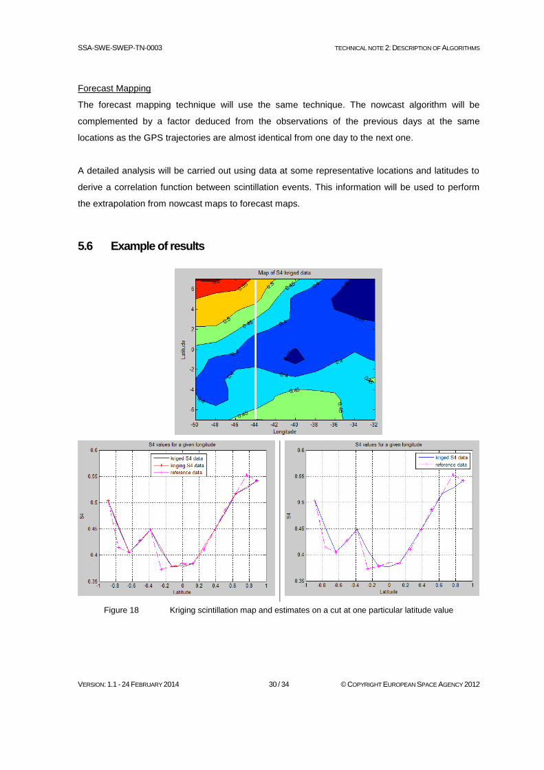
SSA-SWE-SWEP-TN-0003 TECHNICAL NOTE 2: DESCRIPTION OF ALGORITHMS
VERSION: 1.1 - 24 FEBRUARY 2014 30 / 34 © COPYRIGHT EUROPEAN SPACE AGENCY 2012
Forecast Mapping
The forecast mapping technique will use the same technique. The nowcast algorithm will be
complemented by a factor deduced from the observations of the previous days at the same
locations as the GPS trajectories are almost identical from one day to the next one.
A detailed analysis will be carried out using data at some representative locations and latitudes to
derive a correlation function between scintillation events. This information will be used to perform
the extrapolation from nowcast maps to forecast maps.
5.6 Example of results
Figure 18 Kriging scintillation map and estimates on a cut at one particular latitude value

SSA-SWE-SWEP-TN-0003 TECHNICAL NOTE 2: DESCRIPTION OF ALGORITHMS
VERSION: 1.1 - 24 FEBRUARY 2014 31 / 34 © COPYRIGHT EUROPEAN SPACE AGENCY 2012
This example is provided as an illustration of the algorithm capability. The top panel shows a
scintillation map at IPP altitude (350 km), produced by modeling. The mesh size is 1° x 1°. The
modeling result is named reference data in the two below figures.
We have considered the case which will always occurs when we do not have measurements with a
fine mesh but on the contrary with a few points on this grid. The Kriging S4 data (red curve)
represents the curve obtained with the points used in the Kriging algorithm as input data. One point
every two points is skipped. The blue curve shows the result obtained with the Kriging algorithm.
As mentioned this curve minimizes the variance along this line.
Sampled coordinates were used for these plots.
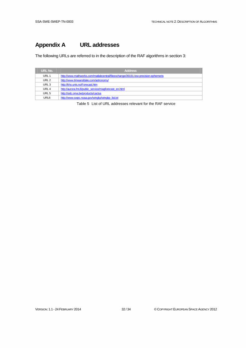
SSA-SWE-SWEP-TN-0003 TECHNICAL NOTE 2: DESCRIPTION OF ALGORITHMS
VERSION: 1.1 - 24 FEBRUARY 2014 32 / 34 © COPYRIGHT EUROPEAN SPACE AGENCY 2012
Appendix A URL addresses
The following URLs are referred to in the description of the RAF algorithms in section 3:
URL No. Address
URL 1 http://www.mathworks.com/matlabcentral/fileexchange/39191-low-precision-ephemeris
URL 2 http://www.timeanddate.com/astronomy/
URL 3 http://kho.unis.no/Forecast.htm
URL 4 http://aurora.fmi.fi/public_service/magforecast_en.html
URL 5 http://sidc.oma.be/products/cactus
URL6 http://www.swpc.noaa.gov/wingkp/wingkp_list.txt
Table 5 List of URL addresses relevant for the RAF service
SSA-SWE-SWEP-TN-0003 TECHNICAL NOTE 2: DESCRIPTION OF ALGORITHMS
VERSION: 1.1 - 24 FEBRUARY 2014 33 / 34 © COPYRIGHT EUROPEAN SPACE AGENCY 2012
Appendix B Alerts
This appendix gives a description of the solar and global geomagnetic activity alerts used in the RAF service.
B.1 NOAA alerts
RAF uses the following alerts from NOAA:
ALTK04---ALTK09: Geomagnetic K index alerts are issued in near real time for K values K=4 or higher, K=5 corresponding to NOAA scale Minor geomagnetic storm, G1. The K index data comes from selected mid- and high-latitude magnetometers, from which the data are available online in real-time.
ALTPX1-ALTPX4: Proton flux alerts are issued for 10MeV and 100MeV protons when the integral flux level exceeds 10, 100, 1000, 10000 or 100000 pfu (proton flux unit = particles per second, steradian and square cm) at geosynchronous orbit observed by GOES satellites. Proton 10 MeV flux threshold of 10 pfu corresponds to the NOAA scale Minor radiation storm, S1.
ALTXMF: X-ray alert is issued when the X-ray flux exceeds the M5 level. M5 level as recorded by the GOES X-ray satellite exceeds 5*10^-5 W/m^2 in the wavelength regime 0.1-0.8 nm. M5 corresponds to the NOAA scale Moderate Radio Black Out, R2.
ALTEF3 alert is issued when the electron 2-MeV Integral flux exceeds 1000 pfu.
B.2 SIDC Halo-CME alert
Halo CME alerts are issued by Solar Influences Data analysis Center (SIDC) when Computer Aided CME Tracking Software (CACTUS) detects a halo or a partial halo CME in SOHO/LASCO (Solar & Heliospheric Observatory / Large Angle and Spectrometric Coronograph) images (see URL 5 in Appendix A). This alert comes with a timing, velocity, propagation and angle estimate of the observed CME. Based on these parameters the plasma cloud's impact on near-Earth space can be estimated.
B.3 FMI/ACE alert
The FMI/ACE alerts give one hour prediction for the range of the magnetic X (north) component (range of X is called RX hereafter) at each of the five RAF stations. More accurately, the service provides two values, min(RX) and max(RX) (2
nd and 3
rd column in Figure 19, below). The RX value for the next coming
hour will lie between these values with 90% probability. Min(RX) and max (RX) are determined from the basis of IMF data collected by the ACE satellite at L1 point during the previous hour. The statistical method used to create the predictions is described in detail in the service web page (see URL 4 in Appendix A). The solar wind data are monitored for the range of magnetic Z-component, wind speed and density, and only negative interplanetary magnetic field is taken to indicate activity. The RX values are divided into five levels (in colour scale green, yellow, orange, red and dark red), from which the three highest levels (orange and red colours) have been observed to be related to appearance of visual aurora. For the RAF stations KEV, MUO, OUJ, HAN and NUR the threshold values for orange color are 326, 303, 167, 77 and 64 nT respectively. The thresholds of RX for the three highest levels correspond to

SSA-SWE-SWEP-TN-0003 TECHNICAL NOTE 2: DESCRIPTION OF ALGORITHMS
VERSION: 1.1 - 24 FEBRUARY 2014 34 / 34 © COPYRIGHT EUROPEAN SPACE AGENCY 2012
about 1.9, 1 and 0.1% tail of the range distribution. The orange colour in the magnetic activity corresponds to the NOAA scale Moderate geomagnetic storm level, G2.
Figure 19 FMI/ACE alert table as shown in the AurorasNow! service (aurora.fmi.fi). Min(RX) and
max(RX) values which are used in the RAF service are given in the 2nd
and 3rd
columns of the Geomagnetic
activity table.
![Software User Manual - ESAswe.ssa.esa.int/DOCS/SSA-DC/SSA-SWE-SWEP-SUM-0001.pdf[AD.29] SWE Portal Services – Software Requirements Specification SSA-SWE-SWEP-SRS-0200 [AD.30] File](https://static.fdocuments.in/doc/165x107/5f8dbc6dab6efb5e327aa85e/software-user-manual-ad29-swe-portal-services-a-software-requirements-specification.jpg)