IMAGE FUSION: A POWERFUL TOOL FOR OBJECT IDENTIFICATION

Filip Sroubek (sroubekf@utia.cas.cz), Jan Flusser (flusser@utia.cas.cz)and Barbara Zitova (zitova@utia.cas.cz)Institute of Information Theory and AutomationAcademy of Sciences of the Czech RepublicPod vodarenskou vezı 4, Praha 8, 182 08, Czech Republic

Abstract. Due to imperfections of imaging devices (optical degradations, limited resolution ofCCD sensors) and instability of the observed scene (object motion, media turbulence), acquiredimages are often blurred, noisy and may exhibit insufficient spatial and/or temporal resolution. Suchimages are not suitable for object detection and recognition. Reliable detection requires recoveringthe original image. If multiple images of the scene are available, this can be achieved by imagefusion.

In this chapter we review the respective methods of image fusion. We address all three ma-jor steps - image registration, blind deconvolution and resolution enhancement. Image registrationbrings the acquired images into spatial alignment, multiframe deconvolution estimates and removesthe blur, and the spatial resolution of the image is increased by so-called superresolution fusion.Superresolution is the main topic of the chapter. We propose a unifying system that simultaneouslyestimates blurs and recovers the original undistorted image, all in high resolution, without any priorknowledge of the blurs and original image. We accomplish this by formulating the problem as con-strained least squares energy minimization with appropriate regularization terms, which guaranteesa close-to-perfect solution.

We demonstrate the performance of the method on many examples, namely on car licenseplate recognition and face recognition. Both of these tasks are of great importance in security andsurveillance systems.

Key words: Image fusion, Multichannel systems, Blind deconvolution, Superresolution, Regular-ized energy minimization

1. Introduction

Imaging devices have limited achievable resolution due to many theoretical andpractical restrictions. An original scene with a continuous intensity functiono[x, y]warps at the camera lens because of the scene motion and/or change of the cameraposition. In addition, several external effects blur images: atmospheric turbulence,camera lens, relative camera-scene motion, etc. We will call these effectsvolatileblurs to emphasize their unpredictable and transitory behavior, yet we will assumethat we can model them as convolution with an unknown point spread function

c© 2006Springer. Printed in the Netherlands.

2 F. SROUBEK ET AL.

(PSF)v[x, y]. This is a reasonable assumption if the original scene is flat andperpendicular to the optical axis. Finally, the CCD discretizes the images andproduces a digitized noisy imageg[i, j] (frame). We refer tog[i, j] as a low-resolution (LR) image, since the spatial resolution is too low to capture all thedetails of the original scene. In conclusion, the acquisition model becomes

g[i, j] = D((v ∗ o[W(n1,n2)])[ x, y]) + n[i, j] , (1)

wheren[i, j] is additive noise andW denotes geometric deformation (spatial warp-ing) of the image. Geometric deformations are partly caused by the fact that theimage is a 2-D projection of a 3-D world, and partly by lens distortions and/ormotion of the sensor during the acquisition.D(·) = S(g ∗ ·) is the decimationoperatorthat models the function of the CCD sensors. It consists of convolutionwith thesensor PSF g[i, j] followed by thesampling operator S, which we defineas multiplication by a sum of delta functions placed on an evenly spaced grid. Theabove model for one single observationg[i, j] is extremely ill-posed. Instead oftaking a single image we can takeK (K > 1) images of the original scene and, inthis way, partially overcome the equivocation of the problem. Hence we write

gk[i, j] = D((vk ∗ o[Wk(n1,n2)])[ x, y]) + nk[i, j] , (2)

wherek = 1, . . . ,K andD remains the same in all the acquisitions. In the perspec-tive of this multiframe model, the original sceneo[x, y] is a single input and theacquired LR imagesgk[i, j] are multiple outputs. The model is therefore called asingle input multiple output (SIMO) formation model. To our knowledge, this isthe most accurate, state-of-the-art model, as it takes all possible degradations intoaccount.

Because of many unknown parameters of the model, it is hard to analyze(automatically or visually) the imagesgk and to detect and recognize objects inthem. A very powerful strategy is offered byimage fusion.

The term fusion means in general an approach to extraction of informationadopted in several domains. The goal of image fusion is to integrate complemen-tary information from all frames into one new image containing information thequality of which cannot be achieved otherwise. Here, the term “better quality”means less blur and geometric distortion, less noise, and higher spatial resolution.We may expect that object detection and recognition will be easier and morereliable when performed on the fused image. Regardless of the particular fusionalgorithm, it is unrealistic to assume that the fused image can recover the originalsceneo[x, y] exactly. A reasonable goal of the fusion is a discrete version ofo[x, y]that has higher spatial resolution than the resolution of the LR images and that isfree of the volatile blurs. In the sequel, we will refer to this fused image as ahighresolution (HR) image f[i, j].

Fusion of images acquired according to the model (2) is a three-stage process– it consists of image registration (spatial alignment), which should compensate

IMAGE FUSION 3

Figure 1. Image fusion in brief: Acquired images (left), registered frames (middle), fused image(right).

for geometric deformationsWk, followed by amultichannel(or multiframe)blinddeconvolution(MBD) and superresolution (SR) fusion. The goal of MBD is toremove the impact of volatile blurs and the aim of SR is to increase spatial res-olution of the fused image by a user-defined factor. While image registration isactually a separate procedure, we integrate both MBD and SR into a single step(see Fig 1), which we callblind superresolution(BSR). The approach presentedin this chapter is one of the first attempts to solve BSR under realistic assumptionswith only little a priori knowledge.

Image registration is a very important step of image fusion, because all MBDand SR methods require either perfectly aligned channels (which is not realistic)or allow at most small shift differences. Thus, the role of registration methods isto suppress large and complex geometric distortions. Image registration in generalis a process of transforming two or more images into a geometrically equivalentform. From the mathematical point of view, it consists of approximatingW−1

kand of resampling the image. For images which are not blurred, registration hasbeen extensively studied in the recent literature (see (Zitova and Flusser, 2003)for a survey). However, blurred images require special registration techniques.They can be, as well as the general-purpose registration methods, divided in twogroups – global and landmark-based ones. Regardless of the particular technique,all feature extraction methods, similarity measures, and matching algorithms usedin the registration process must be insensitive to image blurring.

Global methods do not search for particular landmarks in the images. Theytry to estimate directly the between-channel translation and rotation. In (Mylesand Lobo, 1998) they proposed an iterative method which works well if a goodinitial estimate of the transformation parameters is available. In (Zhang et al.,2000; Zhang et al., 2002) the authors proposed to estimate the registration param-eters by bringing the channels into canonical form. Since blur-invariant moments

4 F. SROUBEK ET AL.

were used to define the normalization constraints, neither the type nor the levelof the blur influences the parameter estimation. In (Kubota et al., 1999) theyproposed a two-stage registration method based on hierarchical matching, wherethe amount of blur is considered as another parameter of the search space. In(Zhang and Blum, 2001) they proposed an iterative multiscale registration basedon optical flow estimation in each scale, claiming that optical flow estimation isrobust to image blurring. All global methods require considerable (or even com-plete) spatial overlap of the channels to yield reliable results, which is their majordrawback.

Landmark-based blur-invariant registration methods have appeared very re-cently, just after the first paper on the moment-based blur-invariant features (Flusseret al., 1996). Originally, these features could only be used for registration of mutu-ally shifted images (Flusser and Suk, 1998), (Bentoutou et al., 2002). The proposalof their rotational-invariant version (Flusser and Zitova, 1999) in combinationwith a robust detector of salient points (Zitova et al., 1999) led to the registrationmethods that are able to handle blurred, shifted and rotated images (Flusser et al.,1999), (Flusser et al., 2003).

Although the above-cited registration methods are very sophisticated and canbe applied almost to all types of images, the results tend to be rarely perfect.The registration error usually varies from subpixel values to a few pixels, so onlyMBD and SR methods sufficiently robust to between-channel misregistration canbe applied to channel fusion. We will assume in the sequel that the LR images areroughly registered and thatWk’s reduce to small translations.

During the last twenty years, blind deconvolution has attracted considerableattention as a separate image processing task. Initial blind deconvolution attemptswere based on single-channel formulations, such as in (Lagendijk et al., 1990;Reeves and Mersereau, 1992; Chan and Wong, 1998; Haindl, 2000). A goodoverview is in (Kundur and Hatzinakos, 1996a; Kundur and Hatzinakos, 1996b).The problem is extremely ill-posed in the single-channel framework and cannotbe resolved in the fully blind form. These methods do not exploit the potential ofmultiframe imaging, because in the single-channel case the missing informationabout the original image in one channel cannot by supplemented by informationobtained from the other channels. Research on intrinsically multichannel methodshas begun fairly recently; refer to (Harikumar and Bresler, 1999; Giannakis andHeath, 2000; Pai and Bovik, 2001; Panci et al., 2003;Sroubek and Flusser, 2003)for a survey and other references. Such MBD methods break the limitations ofprevious techniques and can recover the blurring functions from the degradedimages alone. We further developed the MBD theory in (Sroubek and Flusser,2005) by proposing a blind deconvolution method for images, which might bemutually shifted by unknown vectors. A similar idea is used here as a part of thefusion algorithm to remove volatile blurs and will be explained more in Section 3.

Superresolution has been mentioned in the literature with an increasing fre-

IMAGE FUSION 5

quency in the last decade. The first SR methods did not involve any deblurring;they just tried to register the LR images with subpixel accuracy and then to resam-ple them on a high-resolution grid. A good survey of SR techniques can be foundin (Park et al., 2003; Farsui et al., 2004). Maximum likelihood (ML), maximuma posteriori (MAP), the set theoretic approach using POCS (projection on convexsets), and fast Fourier techniques can all provide a solution to the SR problem. Ear-lier approaches assumed that subpixel shifts are estimated by other means. Moreadvanced techniques, such as in (Hardie et al., 1997; Segall et al., 2004; Woodset al., 2006), include shift estimation in the SR process. Other approaches focuson fast implementation (Farsiu et al., 2004), space-time SR (Shechtman et al.,2005) or SR of compressed video (Segall et al., 2004). Some of the recent SRmethods consider image blurring and involve blur removal. Most of them assumeonly a priori known blurs. However, few exceptions exist. Authors in (Nguyenet al., 2001; Woods et al., 2003) proposed BSR that can handle parametric PSFswith one parameter. This restriction is unfortunately very limiting for most realapplications. Probably the first attempts for BSR with an arbitrary PSF appearedin (Wirawan et al., 1999; Yagle, 2003), where polyphase decomposition of theimages was employed.

Current multiframe blind deconvolution techniques require no or very littleprior information about the blurs, they are sufficiently robust to noise and providesatisfying results in most real applications. However, they can hardly cope with thedownsampling operator, which violates the standard convolution model. On thecontrary, state-of-the-art SR techniques achieve remarkable results in resolutionenhancement in the case of no blur. They accurately estimate the subpixel shiftbetween images but lack any apparatus for calculating the blurs.

We propose a unifying method that simultaneously estimates the volatile blursand HR image without any prior knowledge of the blurs and the original image.We accomplish this by formulating the problem as a minimization of a regularizedenergy function, where the regularization is carried out in both the image and blurdomains. Image regularization is based on variational integrals, and a consequentanisotropic diffusion with good edge-preserving capabilities. A typical example ofsuch regularization is total variation. However, the main contribution of this worklies in the development of the blur regularization term. We show that the blurscan be recovered from the LR images up to small ambiguity. One can considerthis as a generalization of the results proposed for blur estimation in the caseof MBD problems. This fundamental observation enables us to build a simpleregularization term for the blurs even in the case of the SR problem. To tackle theminimization task we use an alternating minimization approach, consisting of twosimple linear equations.

The rest of the chapter is organized as follows. Section 2 outlines the degrada-tion model. In Section 3 we present a procedure for volatile blur estimation. Thiseffortlessly blends in a regularization term of the BSR algorithm as described in

6 F. SROUBEK ET AL.

Section 4. Finally, Section 5 illustrates applicability of the proposed method toreal situations.

2. Mathematical Model

To simplify the notation, we will assume only images and PSFs with squaresupports. An extension to rectangular images is straightforward. Letf [x, y] bean arbitrary discrete image of sizeF × F, thenf denotes an image column vec-tor of sizeF2 × 1 andCA{ f } denotes a matrix that performs convolution offwith an image of sizeA × A. The convolution matrix can have a different outputsize. Adopting the Matlab naming convention, we distinguish two cases: “full”convolution CA{ f } of size (F + A − 1)2 × A2 and “valid” convolutionCv

A{ f }of size (F − A + 1)2 × A2. In both cases the convolution matrix is a Toeplitz-block-Toeplitz (TBT) matrix. In the sequel we will not specify dimensions ofconvolution matrices if it is obvious from the size of the right argument.

Let us assume we haveK different LR frames{gk} (each of sizeG ×G) thatrepresent degraded (blurred and noisy) versions of the original scene. Our goalis to estimate the HR representation of the original scene, which we denoted asthe HR imagef of size F × F. The LR frames are linked with the HR imagethrough a series of degradations similar to those betweeno[x, y] and gk in (2).First f is geometrically warped (Wk), then it is convolved with a volatile PSF (Vk)and finally it is decimated (D). The formation of the LR images in vector-matrixnotation is then described as

gk = DVkWkf + nk , (3)

wherenk is additive noise present in every channel. The decimation matrixD =SU simulates the behavior of digital sensors by first performing convolution withthe U × U sensor PSF (U) and then downsampling (S). The Gaussian functionis widely accepted as an appropriate sensor PSF and it is also used here. Itsjustification is experimentally verified in (Capel, 2004). A physical interpretationof the sensor blur is that the sensor is of finite size and it integrates impinginglight over its surface. The sensitivity of the sensor is highest in the middle anddecreases towards its borders with Gaussian-like decay. Further we assume thatthe subsampling factor (or SR factor, depending on the point of view), denotedby ε, is the same in both x and y directions. It is important to underline thatεis a user-defined parameter. In principle,Wk can be a very complex geometrictransform that must be estimated by image registration or motion detection tech-niques. We have to keep in mind that sub-pixel accuracy ingk’s is necessary forSR to work. Standard image registration techniques can hardly achieve this andthey leave a small misalignment behind. Therefore, we will assume that complexgeometric transforms are removed in the preprocessing step andWk reduces to a

IMAGE FUSION 7

small translation. HenceVkWk = Hk, whereHk performs convolution with theshifted version of the volatile PSFvk, and the acquisition model becomes

gk = DHkf + nk = SUHkf + nk . (4)

The BSR problem then adopts the following form: We know the LR images{gk}

and we want to estimate the HR imagef for the givenSand the sensor blurU. Toavoid boundary effects, we assume that each observationgk captures only a partof f . HenceHk andU are “valid” convolution matricesCv

F{hk} andCvF−H+1{u},

respectively. In general, the PSFshk are of different size. However, we postulatethat they all fit into aH × H support.

In the case ofε = 1, the downsamplingS is not present and we face a slightlymodified MBD problem that has been solved elsewhere (Harikumar and Bresler,1999;Sroubek and Flusser, 2005). Here we are interested in the case ofε > 1,when the downsampling occurs. Can we estimate the blurs as in the caseε = 1?The presence ofS prevents us from using the cited results directly. However, wewill show that conclusions obtained for MBD apply here in a slightly modifiedform as well.

3. Reconstruction of Volatile Blurs

Estimation of blurs in the MBD case (no downsampling) attracted considerableattention in the past. A wide variety of methods were proposed, such as in (Hariku-mar and Bresler, 1999; Giannakis and Heath, 2000), that provide a satisfactorysolution. For these methods to work correctly, certain channel disparity is neces-sary. The disparity is defined as weak co-primeness of the channel blurs, whichstates that the blurs have no common factor except a scalar constant. In otherwords, if the channel blurs can be expressed as a convolution of two subkernelsthen there is no subkernel that is common to all blurs. An exact definition ofweakly co-prime blurs can be found in (Giannakis and Heath, 2000). Many prac-tical cases satisfy the channel co-primeness, since the necessary channel disparityis mostly guaranteed by the nature of the acquisition scheme and random pro-cesses therein. We refer the reader to (Harikumar and Bresler, 1999) for a relevantdiscussion. This channel disparity is also necessary for the BSR case.

Let us first recall how to estimate blurs in the MBD case and then we willshow how to generalize the results for integer downsampling factors. For the timebeing we will omit noisen, until Section 4, where we will address it appropriately.

3.1. THE MBD CASE

The downsampling matrixS is not present in (4) and only convolution binds theinput with the outputs. The acquisition model is of the SIMO type with one

8 F. SROUBEK ET AL.

input channelf and K output channelsgk. Under the assumption of channelco-primeness, we can see that any two correct blurshi andh j satisfy

‖gi ∗ h j − g j ∗ hi‖2 = 0 . (5)

Considering all possible pairs of blurs, we can arrange the above relation into onesystem

N ′h = 0 , (6)

whereh = [hT1 , . . . ,h

TK ]T andN ′ consists of matrices that perform convolution

with gk. In most real situations the correct blur size (we have assumed squaresize H × H) is not known in advance and therefore we can generate the aboveequation for different blur dimensionsH1×H2. The nullity (null-space dimension)ofN ′ is exactly 1 for the correctly estimated blur size. By applying SVD (singularvalue decomposition), we recover precisely the blurs except for a scalar factor.One can eliminate this magnitude ambiguity by stipulating that

∑x,y hk[x, y] = 1,

which is a common brightness preserving assumption. For the underestimatedblur size, the above equation has no solution. If the blur size is overestimated,then nullity(N ′) = (H1 − H + 1)(H2 − H + 1).

3.2. THE BSR CASE

Before we proceed, it is necessary to define precisely the sampling matrixS. LetSε1 denote a 1-D sampling matrix, whereε is the integer subsampling factor. Eachrow of the sampling matrix is a unit vector whose nonzero element is at such aposition that, if the matrix multiplies an arbitrary vectorb, the result of the productis everyε-th element ofb starting fromb1. If the vector length isM then the sizeof the sampling matrix is (M/ε) × M. If M is not divisible byε, we can pad thevector with an appropriate number of zeros to make it divisible. A 2-D samplingmatrix is defined by

Sε := Sε1 ⊗ Sε1 , (7)

where⊗ denotes the matrix direct product (Kronecker product operator). Note thatthe transposed matrix (Sε)T behaves as an upsampling operator that interlaces theoriginal samples with (ε − 1) zeros.

A naive approach, e.g. proposed in (Sroubek and Flusser, 2006; Chen et al.,2005), is to modify (6) in the MBD case by applying downsampling and formu-lating the problem as

minh‖N ′[I K ⊗ SεU]h‖2 , (8)

whereI K is theK × K identity matrix. One can easily verify that the condition in(5) is not satisfied for the BSR case as the presence of downsampling operatorsviolates the commutative property of convolution. Even more disturbing is thefact that minimizers of (8) do not have to correspond to the correct blurs. We are

IMAGE FUSION 9

going to show that if one uses a slightly different approach, reconstruction of thevolatile PSFshk is possible even in the BSR case. However, we will see that someambiguity in the solution ofhk is inevitable.

First, we need to rearrange the acquisition model (4) and construct from theLR imagesgk a convolution matrixG with a predetermined nullity. Then we takethe null space ofG and construct a matrixN , which will contain the correct PSFshk in its null space.

Let E × E be the size of “nullifying” filters. The meaning of this name willbe clear later. DefineG := [G1, . . . ,GK ], whereGk := Cv

E{gk} are “valid” con-volution matrices. Assuming no noise, we can expressG in terms of f , u andhk

asG = SεFUH , (9)

whereH := [CεE{h1}(Sε)T , . . . ,CεE{hK}(Sε)T ] , (10)

U := CεE+H−1{u} andF := CvεE+H+U−2{ f }.

The convolution matrixU has more rows than columns and therefore it is offull column rank (see proof in (Harikumar and Bresler, 1999) for general convo-lution matrices). We assume thatSεF has full column rank as well. This is almostcertainly true for real images ifF has at leastε2-times more rows than columns.Thus Null(G) ≡ Null(H) and the difference between the number of columns androws ofH bounds from below the null space dimension, i.e.,

nullity(G) ≥ KE2 − (εE + H − 1)2 . (11)

SettingN := KE2 − (εE + H − 1)2 andN := Null(G), we visualize the null spaceas

N =

n1,1 . . . n1,N.... . .

...nK,1 . . . nK,N

, (12)

wherenkn is the vector representation of the nullifying filterηkn of sizeE × E,k = 1, . . . ,K andn = 1, . . . ,N. Let ηkn denote upsampledηkn by factorε, i.e.,ηkn := (Sε)Tηkn. Then, we define

N :=

CH{η1,1} . . . CH{ηK,1}...

. . ....

CH{η1,N} . . . CH{ηK,N}

(13)

and conclude thatNh = 0 , (14)

wherehT = [h1, . . . ,hK ]. We have arrived at an equation that is of the same formas (6) in the MBD case. Here we have the solution to the blur estimation problem

10 F. SROUBEK ET AL.

for the BSR case. However, sinceSε is involved, ambiguity of the solution ishigher. Without proofs we provide the following statements. For the correct blursize, nullity(N) = ε4. For the underestimated blur size, (14) has no solution. Forthe overestimated blur sizeH1 × H2, nullity(N) = ε2(H1 − H + ε)(H2 − H + ε).

The conclusion may seem to be pessimistic. For example, forε = 2 the nullityis at least 16, and forε = 3 the nullity is already 81. Nevertheless, Section 4 willshow thatN plays an important role in the regularized restoration algorithm andits ambiguity is not a serious drawback.

It is interesting to note that a similar derivation is possible for rational SRfactorsε = p/q. We downsample the LR images with the factorq, thereby creatingq2K images, and apply thereon the above procedure for the SR factorp.

Another consequence of the above derivation is the minimum necessary num-ber of LR images for the blur reconstruction to work. The condition of theGnullity in (11) implies that the minimum number isK > ε2. For example, forε = 3/2, 3 LR images are sufficient; forε = 2, we need at least 5 LR images toperform blur reconstruction.

4. Blind Superresolution

In order to solve the BSR problem, i.e, determine the HR imagef and volatilePSFshk, we adopt a classical approach of minimizing a regularized energy func-tion. This way the method will be less vulnerable to noise and better posed. Theenergy consists of three terms and takes the form

E(f ,h) =K∑

k=1

‖DHkf − gk‖2 + αQ(f ) + βR(h) . (15)

The first term measures the fidelity to the data and emanates from our acquisitionmodel (4). The remaining two are regularization terms with positive weightingconstantsα andβ that attract the minimum ofE to an admissible set of solutions.The form ofE very much resembles the energy proposed in (Sroubek and Flusser,2005) for MBD. Indeed, this should not come as a surprise since MBD and SRare related problems in our formulation.

RegularizationQ(f ) is a smoothing term of the form

Q(f ) = fTLf , (16)

whereL is a high-pass filter. A common strategy is to use convolution with theLaplacian forL , which in the continuous case corresponds toQ( f ) =

∫|∇ f |2. Re-

cently, variational integralsQ( f ) =∫φ(|∇ f |) were proposed, whereφ is a strictly

convex, nondecreasing function that grows at most linearly. Examples ofφ(s) ares (total variation),

√1+ s2 − 1 (hypersurface minimal function), log(cosh(s)), or

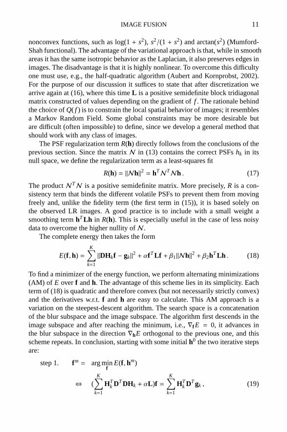
IMAGE FUSION 11

nonconvex functions, such as log(1+ s2), s2/(1 + s2) and arctan(s2) (Mumford-Shah functional). The advantage of the variational approach is that, while in smoothareas it has the same isotropic behavior as the Laplacian, it also preserves edges inimages. The disadvantage is that it is highly nonlinear. To overcome this difficultyone must use, e.g., the half-quadratic algorithm (Aubert and Kornprobst, 2002).For the purpose of our discussion it suffices to state that after discretization wearrive again at (16), where this timeL is a positive semidefinite block tridiagonalmatrix constructed of values depending on the gradient off . The rationale behindthe choice ofQ( f ) is to constrain the local spatial behavior of images; it resemblesa Markov Random Field. Some global constraints may be more desirable butare difficult (often impossible) to define, since we develop a general method thatshould work with any class of images.

The PSF regularization termR(h) directly follows from the conclusions of theprevious section. Since the matrixN in (13) contains the correct PSFshk in itsnull space, we define the regularization term as a least-squares fit

R(h) = ‖Nh‖2 = hTNTNh . (17)

The productNTN is a positive semidefinite matrix. More precisely,R is a con-sistency term that binds the different volatile PSFs to prevent them from movingfreely and, unlike the fidelity term (the first term in (15)), it is based solely onthe observed LR images. A good practice is to include with a small weight asmoothing termhTLh in R(h). This is especially useful in the case of less noisydata to overcome the higher nullity ofN .

The complete energy then takes the form

E(f ,h) =K∑

k=1

‖DHkf − gk‖2 + αfTLf + β1‖Nh‖2 + β2hTLh . (18)

To find a minimizer of the energy function, we perform alternating minimizations(AM) of E over f andh. The advantage of this scheme lies in its simplicity. Eachterm of (18) is quadratic and therefore convex (but not necessarily strictly convex)and the derivatives w.r.t.f andh are easy to calculate. This AM approach is avariation on the steepest-descent algorithm. The search space is a concatenationof the blur subspace and the image subspace. The algorithm first descends in theimage subspace and after reaching the minimum, i.e.,∇f E = 0, it advances inthe blur subspace in the direction∇hE orthogonal to the previous one, and thisscheme repeats. In conclusion, starting with some initialh0 the two iterative stepsare:

step 1. fm = arg minf

E(f ,hm)

⇔ (K∑

k=1

HTk DTDHk + αL )f =

K∑k=1

HTk DTgk , (19)

12 F. SROUBEK ET AL.

step 2. hm+1 = arg minh

E(fm,h)

⇔ ([I K ⊗ FTDTDF] + β1NTN + β2L )h = [I K ⊗ FTDT ]g ,(20)

whereF := CvH{ f }, g := [gT

1 , . . . ,gTK ]T andm is the iteration step. Note that both

steps consist of simple linear equations.EnergyE as a function of both variablesf and h is not convex due to the

coupling of the variables via convolution in the first term of (18). Therefore, it isnot guaranteed that the BSR algorithm reaches the global minimum. In our expe-rience, convergence properties improve significantly if we add feasible regions forthe HR image and PSFs specified as lower and upper bounds constraints. To solvestep 1, we use the method of conjugate gradients (functioncgs in Matlab) andthen adjust the solutionfm to contain values in the admissible range, typically, therange of values ofg. It is common to assume that PSF is positive (hk ≥ 0) and thatit preserves image brightness. We can therefore write the lower and upper boundsconstraints for PSFs ashk ∈ 〈0,1〉H

2. In order to enforce the bounds in step 2, we

solve (20) as a constrained minimization problem (functionfminconin Matlab)rather than using the projection as in step 1. Constrained minimization problemsare more computationally demanding but we can afford it in this case since thesize ofh is much smaller than the size off .

The weighting constantsα andβi depend on the level of noise. If noise in-creases,α andβ2 should increase, andβ1 should decrease. One can use parameterestimation techniques, such as cross-validation (Nguyen et al., 2001) or expecta-tion maximization (Molina et al., 2003), to determine the correct weights. How-ever, in our experiments we set the values manually according to a visual assess-ment. If the iterative algorithm begins to amplify noise, we have underestimatedthe noise level. On the contrary, if the algorithm begins to segment the image, wehave overestimated the noise level.

5. Experiments

This section consists of two parts. In the first one, a set of experiments on syn-thetic data evaluate performance of the BSR algorithm with respect to the SRfactor and compare the reconstruction quality with other methods. The secondpart demonstrates the applicability of the proposed method to real data. Resultsare not evaluated with any measure of reconstruction quality, such as mean-squareerrors or peak signal to noise ratios. Instead we print the results and leave thecomparison to a human eye as we believe that in this case the visual assessment isthe only reasonable method.

In all the experiments the sensor blur is fixed and set to a Gaussian functionof standard deviationσ = 0.34 (relative to the scale of LR images). One shouldunderline that the proposed BSR method is fairly robust to the choice of the Gaus-

IMAGE FUSION 13

1 4 7

1

4

7

a. b.

Figure 2. Simulated data: (a) original 150×230 image; (b) six 7×7 volatile PSFs used to blur theoriginal image.

sian variance, since it can compensate for insufficient variance by automaticallyincluding the missing factor of Gaussian functions in the volatile blurs.

Another potential pitfall that we have to take into consideration is a feasiblerange of SR factors. Clearly, as the SR factorε increases we need more LR imagesand the stability of BSR decreases. In addition, rational SR factorsp/q, wherep and q are incommensurable and large regardless of the effective value ofε,also make the BSR algorithm unstable. It is the numeratorp that determines theinternal SR factor used in the algorithm. Hence we limit ourselves toε between 1and 2.5, such as 3/2, 5/3, 2, etc., which is sufficient in most practical applications.

5.1. SIMULATED DATA

First, let us demonstrate the BSR performance with a simple experiment. A 150×

230 image in Fig. 2.a blurred with the six masks in Fig. 2.b and downsampledwith factor 2 generated six LR images. In this case, registration is not necessarysince the synthetic data are precisely aligned. Using the LR images as an input, weestimated the original HR image with the proposed BSR algorithm forε = 1.25and 1.75. In Fig. 3 one can compare the results printed in their original size. TheHR image forε = 1.25 (Fig. 3.b) has improved significantly on the LR imagesdue to deconvolution, however some details on the column are still distorted. Forthe SR factor 1.75, the reconstructed image in Fig. 3.c is almost perfect.

Next we compare performance of the BSR algorithm with two methods: in-terpolation technique and state-of-the-art SR method. The former technique con-sists of the MBD method proposed in (Sroubek and Flusser, 2005) followed by

14 F. SROUBEK ET AL.

a. LR b. ε = 1.25 c. ε = 1.75

Figure 3. BSR of simulated data: (a) one of six LR images with the downsampling factor 2; (b)BSR forε = 1.25; (c) BSR forε = 1.75.

standard bilinear interpolation (BI) resampling. The MBD method first removesvolatile blurs and then BI of the deconvolved image achieves the desired spatialresolution. The latter method, which we will call herein a “standard SR algo-rithm”, is a MAP formulation of the SR problem proposed, e.g., in (Hardie et al.,1997; Segall et al., 2004). This method uses a MAP framework for the joint es-timation of image registration parameters (in our case only translation) and theHR image, assuming only the sensor blur (U) and no volatile blurs. For an imageprior, we use edge preserving Huber Markov Random Fields (Capel, 2004).

In the case of BSR, Section 3 has shown that two distinct approaches existfor blur estimation. Either we use the naive approach in (8) that directly utilizesthe MBD formulation, or we apply the intrinsically SR approach summarized in(14). Altogether we have thus four distinct methods for comparison: standard SRapproach, MBD with interpolation, BSR with naive blur regularization and BSRwith intrinsic blur regularization. Using the original image and PSFs in Fig. 2,six LR images (see one LR image in Fig. 3.a) were generated as in the firstexperiment, only this time we added white Gaussian noise with SNR= 50dB1.

Estimated HR images and volatile blurs for all four methods are in Fig. 4.The standard SR approach in Fig. 4.a gives unsatisfactory results, since heavyblurring is present in the LR images and the method assumes only the sensorblur and no volatile blurs. (For this reason, we do not show volatile blurs in thiscase). The MBD method in Fig. 4.b ignores the decimation operator and thusthe estimated volatile blurs are similar to LR projections of the original blurs.Despite the fact that blind deconvolution in the first stage performed well, many

1 The signal-to-noise ratio is defined as SNR= 10 log(σ2f /σ

2n), whereσ f andσn are the image

and noise standard deviations, respectively.

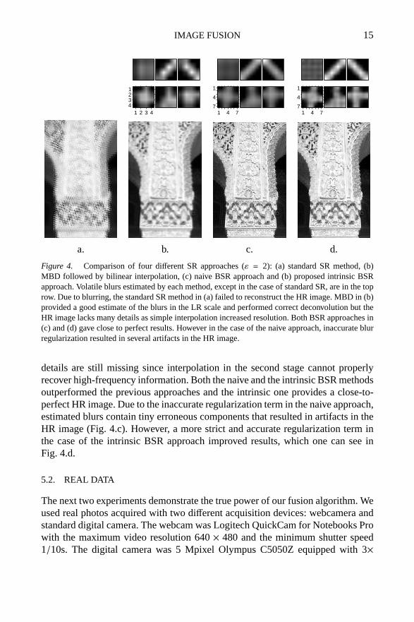
IMAGE FUSION 15

1 2 3 4

1234

1 4 7

1

4

71 4 7

1

4

7

a. b. c. d.

Figure 4. Comparison of four different SR approaches (ε = 2): (a) standard SR method, (b)MBD followed by bilinear interpolation, (c) naive BSR approach and (b) proposed intrinsic BSRapproach. Volatile blurs estimated by each method, except in the case of standard SR, are in the toprow. Due to blurring, the standard SR method in (a) failed to reconstruct the HR image. MBD in (b)provided a good estimate of the blurs in the LR scale and performed correct deconvolution but theHR image lacks many details as simple interpolation increased resolution. Both BSR approaches in(c) and (d) gave close to perfect results. However in the case of the naive approach, inaccurate blurregularization resulted in several artifacts in the HR image.

details are still missing since interpolation in the second stage cannot properlyrecover high-frequency information. Both the naive and the intrinsic BSR methodsoutperformed the previous approaches and the intrinsic one provides a close-to-perfect HR image. Due to the inaccurate regularization term in the naive approach,estimated blurs contain tiny erroneous components that resulted in artifacts in theHR image (Fig. 4.c). However, a more strict and accurate regularization term inthe case of the intrinsic BSR approach improved results, which one can see inFig. 4.d.

5.2. REAL DATA

The next two experiments demonstrate the true power of our fusion algorithm. Weused real photos acquired with two different acquisition devices: webcamera andstandard digital camera. The webcam was Logitech QuickCam for Notebooks Prowith the maximum video resolution 640× 480 and the minimum shutter speed1/10s. The digital camera was 5 Mpixel Olympus C5050Z equipped with 3×

16 F. SROUBEK ET AL.

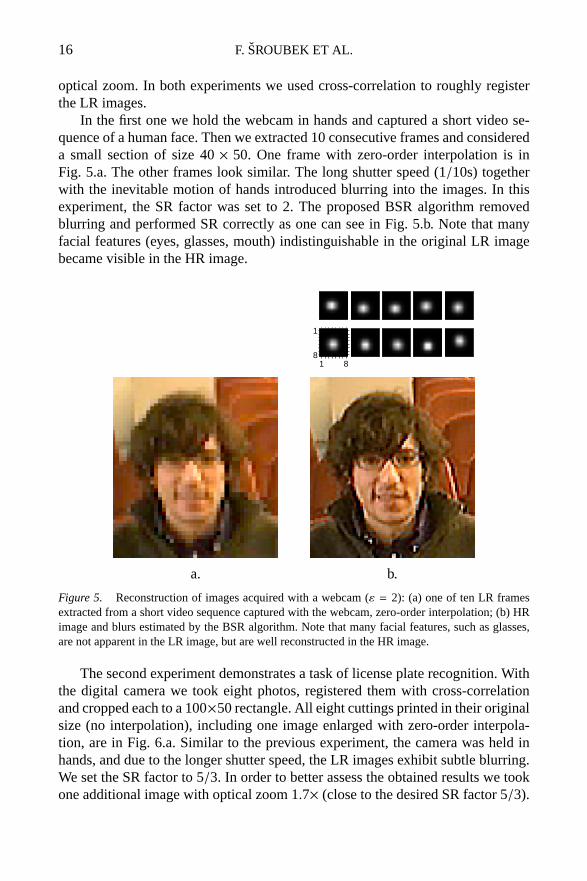
optical zoom. In both experiments we used cross-correlation to roughly registerthe LR images.

In the first one we hold the webcam in hands and captured a short video se-quence of a human face. Then we extracted 10 consecutive frames and considereda small section of size 40× 50. One frame with zero-order interpolation is inFig. 5.a. The other frames look similar. The long shutter speed (1/10s) togetherwith the inevitable motion of hands introduced blurring into the images. In thisexperiment, the SR factor was set to 2. The proposed BSR algorithm removedblurring and performed SR correctly as one can see in Fig. 5.b. Note that manyfacial features (eyes, glasses, mouth) indistinguishable in the original LR imagebecame visible in the HR image.

1 8

1

8

a. b.

Figure 5. Reconstruction of images acquired with a webcam (ε = 2): (a) one of ten LR framesextracted from a short video sequence captured with the webcam, zero-order interpolation; (b) HRimage and blurs estimated by the BSR algorithm. Note that many facial features, such as glasses,are not apparent in the LR image, but are well reconstructed in the HR image.

The second experiment demonstrates a task of license plate recognition. Withthe digital camera we took eight photos, registered them with cross-correlationand cropped each to a 100×50 rectangle. All eight cuttings printed in their originalsize (no interpolation), including one image enlarged with zero-order interpola-tion, are in Fig. 6.a. Similar to the previous experiment, the camera was held inhands, and due to the longer shutter speed, the LR images exhibit subtle blurring.We set the SR factor to 5/3. In order to better assess the obtained results we tookone additional image with optical zoom 1.7× (close to the desired SR factor 5/3).

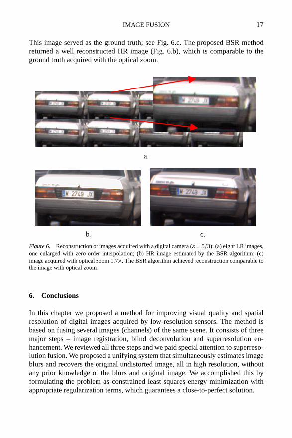
IMAGE FUSION 17

This image served as the ground truth; see Fig. 6.c. The proposed BSR methodreturned a well reconstructed HR image (Fig. 6.b), which is comparable to theground truth acquired with the optical zoom.

a.

b. c.

Figure 6. Reconstruction of images acquired with a digital camera (ε = 5/3): (a) eight LR images,one enlarged with zero-order interpolation; (b) HR image estimated by the BSR algorithm; (c)image acquired with optical zoom 1.7×. The BSR algorithm achieved reconstruction comparable tothe image with optical zoom.

6. Conclusions

In this chapter we proposed a method for improving visual quality and spatialresolution of digital images acquired by low-resolution sensors. The method isbased on fusing several images (channels) of the same scene. It consists of threemajor steps – image registration, blind deconvolution and superresolution en-hancement. We reviewed all three steps and we paid special attention to superreso-lution fusion. We proposed a unifying system that simultaneously estimates imageblurs and recovers the original undistorted image, all in high resolution, withoutany prior knowledge of the blurs and original image. We accomplished this byformulating the problem as constrained least squares energy minimization withappropriate regularization terms, which guarantees a close-to-perfect solution.

18 F. SROUBEK ET AL.

Showing the good performance of the method on real data, we demonstratedits capability to improve the image quality significantly and, consequently, tomake the task of object detection and identification much easier for human ob-servers as well as for automatic systems. We envisage the application of theproposed method in security and surveillance systems.

Acknowledgements

This work has been supported by Czech Ministry of Education under project No.1M0572 (Research Center DAR), and by the Grant Agency of the Czech Republicunder project No. 102/04/0155.

References

Aubert, G. and Kornprobst, P. (2002)Mathematical Problems in Image Processing, New York,Springer Verlag.

Bentoutou, Y., Taleb, N., Mezouar, M., Taleb, M., and Jetto, L. (2002) An invariant approach forimage registration in digital subtraction angiography,Pattern Recognition35, 2853–2865.

Capel, D. (2004)Image Mosaicing and Super-Resolution, New York, Springer.Chan, T. and Wong, C. (1998) Total variation blind deconvolution,IEEE Trans. Image Processing

7, 370–375.Chen, Y., Luo, Y., and Hu, D. (2005) A general approach to blind image super-resolution using a

PDE framework, InProc. SPIE, Vol. 5960, pp. 1819–1830.Farsiu, S., Robinson, M., Elad, M., and Milanfar, P. (2004) Fast and robust multiframe super

resolution,IEEE Trans. Image Processing13, 1327–1344.Farsui, S., Robinson, D., Elad, M., and Milanfar, P. (2004) Advances and challenges in super-

resolution,Int. J. Imag. Syst. Technol.14, 47–57.Flusser, J., Boldys, J., and Zitova, B. (2003) Moment forms invariant to rotation and blur in arbitrary

number of dimensions,IEEE Transactions on Pattern Analysis and Machine Intelligence25,234–246.

Flusser, J. and Suk, T. (1998) Degraded image analysis: an invariant approach,IEEE Trans. PatternAnalysis and Machine Intelligence20, 590–603.

Flusser, J., Suk, T., and Saic, S. (1996) Recognition of blurred images by the method of moments,IEEE Trans. Image Processing5, 533–538.

Flusser, J. and Zitova, B. (1999) Combined invariants to linear filtering and rotation,Intl. J. PatternRecognition Art. Intell.13, 1123–1136.

Flusser, J., Zitova, B., and Suk, T. (1999) Invariant-based registration of rotated and blurred images,In I. S. Tammy (ed.),Proceedings IEEE 1999 International Geoscience and Remote SensingSymposium, Los Alamitos, pp. 1262–1264, IEEE Computer Society.

Giannakis, G. and Heath, R. (2000) Blind identification of multichannel FIR blurs and perfect imagerestoration,IEEE Trans. Image Processing9, 1877–1896.

Haindl, M. (2000) Recursive model-based image restoration, InProceedings of the 15th Interna-tional Conference on Pattern Recognition, Vol. III, pp. 346–349, IEEE Press.

Hardie, R., Barnard, K., and Armstrong, E. (1997) Joint MAP registration and high-resolution imageestimation using a sequence of undersampled images,IEEE Trans. Image Processing6, 1621–1633.

IMAGE FUSION 19

Harikumar, G. and Bresler, Y. (1999) Perfect blind restoration of images blurred by multiple filters:theory and efficient algorithms,IEEE Trans. Image Processing8, 202–219.

Kubota, A., Kodama, K., and Aizawa, K. (1999) Registration and blur estimation methods for multi-ple differently focused images, InProceedings International Conference on Image Processing,Vol. II, pp. 447–451.

Kundur, D. and Hatzinakos, D. (1996)a Blind image deconvolution,IEEE Signal ProcessingMagazine13, 43–64.

Kundur, D. and Hatzinakos, D. (1996)b Blind image deconvolution revisited,IEEE SignalProcessing Magazine13, 61–63.

Lagendijk, R., Biemond, J., and Boekee, D. (1990) Identification and restoration of noisy blurredimages using the expectation-maximization algorithm,IEEE Trans. Acoust. Speech SignalProcess.38, 1180–1191.

Molina, R., Vega, M., Abad, J., and Katsaggelos, A. (2003) Parameter estimation in Bayesian high-resolution image reconstruction with multisensors,IEEE Trans. Image Processing12, 1655–1667.

Myles, Z. and Lobo, N. V. (1998) Recovering affine motion and defocus blur simultaneously,IEEETrans. Pattern Analysis and Machine Intelligence20, 652–658.

Nguyen, N., Milanfar, P., and Golub, G. (2001) Efficient generalized cross-validation with ap-plications to parametric image restoration and resolution enhancement,IEEE Trans. ImageProcessing10, 1299–1308.

Pai, H.-T. and Bovik, A. (2001) On eigenstructure-based direct multichannel blind image restora-tion, IEEE Trans. Image Processing10, 1434–1446.

Panci, G., Campisi, P., Colonnese, S., and Scarano, G. (2003) Multichannel blind image deconvolu-tion using the bussgang algorithm: spatial and multiresolution approaches,IEEE Trans. ImageProcessing12, 1324–1337.

Park, S., Park, M., and Kang, M. (2003) Super-resolution image reconstruction: a technicaloverview, IEEE Signal Proc. Magazine20, 21–36.

Reeves, S. and Mersereau, R. (1992) Blur identification by the method of generalized cross-validation, IEEE Trans. Image Processing1, 301–311.

Segall, C., Katsaggelos, A., Molina, R., and Mateos, J. (2004) Bayesian resolution enhancement ofcompressed video,IEEE Trans. Image Processing13, 898–911.

Shechtman, E., Caspi, Y., and Irani, M. (2005) Space-time super-resolution,IEEE Trans. PatternAnalysis and Machine Intelligence27, 531–545.

Sroubek, F. and Flusser, J. (2003) Multichannel blind iterative image restoration,IEEE Trans. ImageProcessing12, 1094–1106.

Sroubek, F. and Flusser, J. (2005) Multichannel blind deconvolution of spatially misaligned images,IEEE Trans. Image Processing14, 874–883.

Sroubek, F. and Flusser, J. (2006) Resolution enhancement via probabilistic deconvolution ofmultiple degraded images,Pattern Recognition Letters27, 287–293.

Wirawan, Duhamel, P., and Maitre, H. (1999) Multi-channel high resolution blind image restoration,In Proc. IEEE ICASSP, pp. 3229–3232.

Woods, N., Galatsanos, N., and Katsaggelos, A. (2003) EM-based simultaneous registration,restoration, and interpolation of super-resolved images, InProc. IEEE ICIP, Vol. 2, pp.303–306.

Woods, N., Galatsanos, N., and Katsaggelos, A. (2006) Stochastic methods for joint registration,restoration, and interpolation of multiple undersampled images,IEEE Trans. Image Processing15, 201–213.

Yagle, A. (2003) Blind superresolution from undersampled blurred measurements, InAdvanced

20 F. SROUBEK ET AL.

Signal Processing Algorithms, Architectures, and Implementations XIII, Vol. 5205, Bellingham,pp. 299–309, SPIE.

Zhang, Y., Wen, C., and Zhang, Y. (2000) Estimation of motion parameters from blurred images,Pattern Recognition Letters21, 425–433.

Zhang, Y., Wen, C., Zhang, Y., and Soh, Y. C. (2002) Determination of blur and affine combinedinvariants by normalization,Pattern Recognition35, 211–221.

Zhang, Z. and Blum, R. (2001) A hybrid image registration technique for a digital camera imagefusion application,Information Fusion2, 135–149.

Zitova, B. and Flusser, J. (2003) Image registration methods: a survey,Image and Vision Computing21, 977–1000.

Zitova, B., Kautsky, J., Peters, G., and Flusser, J. (1999) Robust detection of significant points inmultiframe images,Pattern Recognition Letters20, 199–206.