Squares of Random Linear Codes

Ignacio Cascudo∗, Ronald Cramer†, Diego Mirandola‡and Gilles Zemor§

January 14, 2015

Abstract

Given a linear code C, one can define the d-th power of C as thespan of all componentwise products of d elements of C. A power of Cmay quickly fill the whole space. Our purpose is to answer the follow-ing question: does the square of a code “typically” fill the whole space?We give a positive answer, for codes of dimension k and length roughly12k

2 or smaller. Moreover, the convergence speed is exponential if thedifference k(k+ 1)/2−n is at least linear in k. The proof uses randomcoding and combinatorial arguments, together with algebraic tools in-volving the precise computation of the number of quadratic forms of agiven rank, and the number of their zeros.Keywords: Error-correcting codes, Schur-product codes, Randomcodes, Quadratic forms.

∗Aarhus University, Denmark. Email: ignacio@cs.au.dk.†CWI Amsterdam and the Mathematical Institute, Leiden University, The Nether-

lands. Email: cramer@cwi.nl, cramer@math.leidenuniv.nl.‡CWI Amsterdam and Mathematical Institute, Leiden University, The Netherlands,

and Institut de Mathematiques de Bordeaux, UMR 5251, Universite de Bordeaux, France.Email: diego@cwi.nl.§Institut de Mathematiques de Bordeaux, UMR 5251, Universite de Bordeaux, France.

Email: zemor@math.u-bordeaux.fr.I. Cascudo acknowledges support from the Danish National Research Foundation and

The National Science Foundation of China (under the grant 61361136003) for the Sino-Danish Center for the Theory of Interactive Computation and from the Center for Re-search in Foundations of Electronic Markets (CFEM), supported by the Danish StrategicResearch Council. Moreover, the research was partially carried out while I. Cascudowas at CWI Amsterdam, The Netherlands, supported by STW Sentinels program underProject 10532 and by Cramer’s NWO VICI Grant Mathematics of Secure Computation.D. Mirandola acknowledges the support of the ALGANT-DOC programme.

Material in this paper was presented at the “Mathematics of Information-TheoreticCryptography” workshop, Leiden, May 13-25 2013 and at the “Algebra, Codes and Net-works” workshop, Bordeaux, June 16-20 2014. To appear on IEEE Transactions on Infor-mation Theory.

1

1 Introduction

Let K be a field and denote by ∗ the coordinatewise product of vectors ofKn, so that:

(x1, . . . , xn) ∗ (y1, . . . , yn) = (x1y1, . . . , xnyn).

When V and W are subspaces of Kn let us denote similarly by V ∗W thesubspace generated by all ∗-products of vectors of V and W , i.e. V ∗W :=〈x ∗ y : x ∈ V, y ∈ W 〉. We also use the shorthand V ∗1 = V , V ∗2 := V ∗ Vand define inductively the powers of V , V ∗d := V ∗ V ∗(d−1) for d > 1.

When K = Fq is a finite field and C is a q-ary linear code, asking whatare the possible parameters of the linear code C∗2 arises in a number ofdifferent contexts and has attracted a lot of attention recently. Possibly oneof the earliest appearances of this question in coding theory goes back to [28]where it is relevant to the notion of error-locating pairs used for algebraicdecoding.

“Products” and “squares” of codes are the primary focus of work onsecret sharing [8, 3, 4, 5] and its application to secure multi-party computa-tion [14]. To share a secret vector s ∈ Fkq among n players using a linear code

C ⊆ Fn+kq , one standardly chooses a random codeword with some fixed k-tuple of coordinates equal to s: the other coordinates are the shares. Whentwo secrets s and t are shared in this way, summing coordinatewise the sharevectors gives naturally a share vector of the coordinatewise sum s+ t of thesecrets. When one considers the ∗-product of the share vectors, one obtainsa share of the product s∗t, but for a different secret-sharing scheme, namelythat associated to the ∗-product code C∗2. Since the parameters of a codeare relevant to the associated secret-sharing scheme, studying the parame-ters of C∗2 becomes important. More precisely, interest is focused on familiesof linear codes (Ci)i∈N of unbounded length, such that the families of thedual codes (C⊥i )i∈N and of the squares (C∗2i )i∈N are asymptotically good. Afamily of codes satisfying this property yields linear secret-sharing schemeson arbitrarily many players with good parameters (privacy, reconstruction,multiplication) [3]. Such families were first constructed, over almost all fi-nite fields, in [8] using techniques from algebraic geometry (asymptoticallygood towers of algebraic function fields). This work was subsequently ex-tended in [3, 4] involving novel algebraic-geometric ideas. We remark thatno elementary construction is known so far.

Secret sharing has as main motivation and application secure multi-partycomputation (MPC). Any linear secret-sharing scheme yields an MPC pro-tocol [14], and the family of all malicious coalitions of players the protocolcan tolerate depends on the parameters of the LSSS listed above.

Besides its original application, the result of [8] played a central rolein the paper [22] on the “secure MPC in the head” paradigm: here secure

2

MPC is used as an abstract primitive for efficient two-party cryptography.1

Among other subsequent fundamental results, let us mention that asymp-totically good codes whose dual and square are also asymptotically good arean essential ingredient in the recent constructions of efficient unconditionallysecure oblivious transfer protocols from noisy channels [21, 27].

The same issue is also pertinent to algebraic complexity theory: thereone wishes to express multiplication in the extension field Fqm through abilinear algorithm involving a small number of multiplications in Fq, see[1, 7, 29, 6] for recent developments.

Motivated in part by these applications, asymptotically good codes whosesquares are also asymptotically good (and we impose no conditions on theduals) have been shown to exist for all finite fields in [30]. This constructioncarefully combines algebraic geometric codes that have asymptotically goodhigher powers, which can be constructed over large enough finite fields, witha field descent concatenation technique. Again, no elementary constructionis known in this case.

Powers of linear codes also turn up in lattice constructions, as was re-cently elaborated on in [23]. If C is a binary linear code, then, abusingnotation by identifying C with its natural lift in Zn, the most natural latticeconstruction from C is Λ = C+2Zn (construction A in Conway and Sloane’sterminology [10]). The minimum Euclidean norm of a lattice vector is thenmin(

√dmin(C), 2), where dmin(C) is the minimum Hamming distance of the

code C. If one wishes to generate from the code C a lattice with larger Eu-clidean distance, one may try to construct the lattice generated by C+4Zn:a close look shows that this lattice actually equals

C + 2C∗2 + 4Zn

and its minimum Euclidean norm is

min(√

dmin(C), 2√dmin(C∗2), 4

).

One may generalize the construction to C + 2C∗2

+ 4C∗4 + 8Zn and so on,or more generally to (construction D [10]) C0 + 2C1 + · · ·+ 2`−1C`−1 + 2`Zn,which is a lattice if and only if C∗2j ⊂ Cj+1, a fact not usually explicitelystated in the literature.

Finally, there has been some recent use of ∗-squares in the cryptanalysisof variants of the McEliece cryptosystem [19, 11, 12, 13]. The idea thatis exploited is that Goppa codes have a ∗-square that has a substantiallysmaller dimension than typical random linear codes: this allows to build adistinguisher which can be used to attack the cryptosystem.

The motivation for a systematic code-theoretic study of ∗-squares istherefore quite strong. For a wide collection of results on the topic see [31]

1For an extensive treatment of the interplay between secure multiparty computation,(arithmetic) secret sharing, codes and algebraic geometry, please consult [15].

3

and references therein. With a view to contribute to such an endeavour,our concern in the present work is with the dimension of squares of randomlinear codes: we see that this is especially relevant in particular to the lastapplication to cryptanalysis.

Since a generating set of vectors for the square of a code C of dimension kcan be constructed by taking all possible k(k+1)/2 products of two elementsof a basis of the code C, it is reasonable to expect that a randomly chosencode of block length n < k(k + 1)/2 has a ∗-square which fills up the wholespace, i.e. C∗2 = Fnq . However, linear relations between products of elementsof C are not typically independent random events, and one has to overcomea certain number of obstacles to prove such a statement. Our main resultis indeed to show that when the difference k(k + 1)/2 − n goes to infinityas a function of k, however slowly, the probability that a random code oflength n and dimension k has a square different from Fnq goes to zero. Wealso study the speed of convergence, which is exponential if the differencek(k+1)/2−n is at least linear in k, and the limiting case n = k(k+1)/2. Weshall also consider the slightly easier case when the blocklength n is suchthat n ≥ k(k + 1)/2: we obtain that with probability tending to 1 whenn − k(k + 1)/2 goes to infinity, the dimension of the square of the randomcode is exactly k(k + 1)/2. Again, this convergence is exponentially fastif n − k(k + 1)/2 is at least linear in k. Previously, the best-known facton this problem was given by Faugere et al. in [19] who proved that forn ≥ k(k + 1)/2 and for any function ω(k) that goes to infinity with k, thedimension of the square of the random code is at least k(k + 1)/2 − kω(k)with probability tending to 1 when k goes to infinity.

Our techniques break significantly with the approach of [19] and combinethe study of the dual distance of the square of a random code, and thedistribution of zeros of random quadratic forms. In the next section wedescribe our results precisely and give an overview of our proofs and thestructure of the paper.

2 Overview

Throughout this paper, q denotes a fixed prime power and Fq a field with qelements.

We first define the probabilistic model we shall work with. For all positiveintegers n ≥ k, we define C(n, k) to be the family of all [n, k]-codes over Fqwhose first k coordinates make up an information set: equivalently, membersof C(n, k) have a generator matrix which can be written in systematic form,i.e. as

G =

1. . .

1

A

,

4

for some k× (n−k) matrix A. We endow C(n, k) with the uniform distribu-tion. Since codes of C(n, k) are in one-to-one correspondence with k×(n−k)matrices A, choosing a random element of C(n, k) amounts to choosing arandom uniform matrix A.

Remark 2.1. There are several possible choices for the probabilistic model.An alternative way of choosing a random code consists of choosing its gen-erator matrix uniformly at random among all k × n matrices. Yet anotheralternative is to consider the uniform distribution among all codes of lengthn and dimension k. The first alternative probability distribution has thedisadvantage that the resulting code may be of dimension < k. The secondalternative distribution is perhaps the most theoretically elegant but makesit somewhat cumbersome to use the puncturing arguments that we will workwith, hence the above choice of a probabilistic model. In Section 6 we shallargue however that our results are not altered significantly under these al-ternative probability distributions.

Our main result is:

Main Theorem 2.2. Let n : N→ N be such that k(k+ 1)/2 ≥ n(k) ≥ k forall k ∈ N and define t : N → N, t(k) := k(k + 1)/2− n(k). Then there existconstants γ, δ ∈ R>0 such that, for all large enough k,

Pr(C∗2 = Fn(k)q ) ≥ 1− 2−γk − 2−δt(k),

where C is chosen uniformly at random from C(n(k), k).

For lengths n that are larger than k(k + 1)/2, we also have:

Theorem 2.3. Let n : N→ N be such that n(k) ≥ k(k + 1)/2 for all k ∈ Nand define s : N→ N, s(k) := n(k)−k(k+1)/2. Then there exists a constantδ ∈ R>0 such that, for all large enough k,

Pr

(dimC∗2 =

k(k + 1)

2

)≥ 1− 2−δs(k),

where C is chosen uniformly at random from C(n(k), k).

Strangely enough, Theorems 2.2 and 2.3 are not quite symmetrical. Inparticular the term 2−γk is absent from the statement of Theorem 2.3 butcan not be avoided in Theorem 2.2: this is because with probability at least1/qk, the random matrix G will contain a column of zeros, or two identical

columns, in which case the square C∗2 can not be equal to Fn(k)q . The twotheorems will not require exactly the same methods and Theorem 2.2 willneed more work than Theorem 2.3. We shall deal with them separately.

Our first step towards establishing Theorem 2.2 will be to estimate theexpected minimum distance of the dual of the square of a random code oflength k(k + 1)/2. Specifically, we shall prove:

5

Proposition 2.4. There exist constants (depending only on q) c, c ∈ R>0

such that, for all large enough k, if C is chosen uniformly at random fromC(k(k + 1)/2, k) then

Pr

(dmin((C∗2)

⊥) ≤ c · k(k + 1)

2

)≤ 2−ck.

This last proposition enables us to use puncturing arguments. In ourprobabilistic model, a random code of length n can be obtained by firstchoosing a random code of length n + t and then puncturing t times ona random position. The probability that a punctured code has the samedimension as the original code is well-separated from zero whenever thedual distance of the original code is large enough. This fact will be enoughin itself to establish the following weaker version of Main Theorem 2.2.

Theorem 2.5. There exist constants (depending only on q) c, c ∈ R>0 suchthat, if n : N→ N satisfies

k ≤ n(k) ≤ c · k(k + 1)

2

for all k ∈ N then, for all large enough k,

Pr(C∗2 = Fn(k)q ) ≥ 1− 2−ck,

where C is chosen uniformly at random from C(n(k), k).

However, in order to deal with block lengths that approach the upperbound k(k + 1)/2 on the dimension of the square of C, and prove the full-fledged Main Theorem 2.2, we need some additional ingredients.

Given an [n, k]-code C and denoting by π1, . . . , πn ∈ Fkq the columns ofa generator matrix of C, define the linear map

evC : Quad(Fkq ) → Fnq ,Q 7→ (Q(π1), . . . , Q(πn))

where Quad(Fkq ) denotes the vector space of quadratic forms on Fkq . Thenone can see that the image of evC does not depend on the choice of agenerator matrix of C, and it is equal to C∗2, see [31, §1.31]. In particular,C∗2 = Fnq if and only if evC is surjective. Moreover, by basic linear algebraC∗2 = Fnq if and only if

dim ker evC = dim Quad(Fkq )− n =k(k + 1)

2− n.

So it makes sense to focus on this kernel. We view its cardinality as arandom variable, with distribution induced by the uniform distribution ofC over C(n, k): formally, for all positive integers n ≥ k we define

X(n, k) := | ker evC |.

Our main intermediate result, of interest in its own right, is:

6

Theorem 2.6. We have that

limk→∞

E[X

(k(k + 1)

2, k

)]= 2.

A simple use of Markov’s inequality will then give us that, for a randomcode C of length k(k + 1)/2, the probability that the codimension of C∗2

does not exceed `,

Pr

(dimC∗2 ≥ k(k + 1)

2− `)

tends to 1 when ` goes to infinity, furthermore exponentially fast if ` is linearin k. Puncturing arguments, again relying on Proposition 2.4, will enableus to conclude the proof of Theorem 2.2 when the block length n is wellseparated from k(k + 1)/2.

As a by-product, Theorem 2.6 also enables us to deal easily with thecase when n ≥ k(k + 1)/2. Theorem 2.3 will follow as a straightforwardconsequence.

We conclude this overview by giving a rough idea of the proof of Theo-rem 2.6. It involves computing the number of zeros of a quadratic form ofgiven rank and the number of quadratic forms of given rank; the results weneed are stated precisely in Section 4 and a detailed proof is provided in theAppendix.

By definition, for all positive integers m ≥ k we have

E[X(m, k)] =

= E[|{Q ∈ Quad(Fkq ) : Q(π1) = · · · = Q(πm) = 0}|],

where we can assume that, for i = 1, . . . , k, πi = ei is the i-th unit vectorwhile πk+1, . . . , πm ∈ Fkq have independent, uniform distribution over Fkq , bydefinition of the family C(m, k) and our probabilistic model.

Note that the conditions Q(e1) = · · · = Q(ek) = 0 are independent (inthe sense of linear algebra), hence the subspace

S := {Q ∈ Quad(Fkq ) : Q(e1) = · · · = Q(ek) = 0}

of Quad(Fkq ) has dimension k(k − 1)/2. Moreover, as πk+1, . . . , πm ∈ Fkq areindependent (in the sense of probability), we have

Pr(Q(πk+1) = · · · = Q(πm) = 0) =

= Pr(Q(πk+1) = 0)m−k =

(|Z(Q)|qk

)m−kfor any Q ∈ Quad(Fkq ). Here Z(Q) denotes the zero set of Q. Finally, by

7

linearity of the expectation we have

E[X(m, k)] =

= E[|{Q ∈ S : Q(πk+1) = · · · = Q(πm) = 0}|] =

=∑Q∈S

(|Z(Q)|qk

)m−k. (1)

Now if it were true (it is not) that all non-zero quadratic forms on Fkqhave qk−1 zeros, we would have, when we set m = k(k + 1)/2,

E[X(m, k)] = 1 +1

qm−k(q

k(k−1)2 − 1) −→ 2

“proving” Theorem 2.6. However, even though it is false that all non-zeroquadratic forms on Fkq have qk−1 zeros, this still holds “on average”: roughly

speaking, most quadratic forms have qk−1 zeros, quadratic forms whosenumber of zeros is far from this value are those of small rank, and thenumber of such forms is so small that it contributes almost nothing to theexpectation. In other words, the expectation behaves as if it were true thatall non zero quadratic forms on Fkq have qk−1 zeros.

The rest of the paper is organized as follows. Section 3 is devoted toproving Proposition 2.4 and Theorem 2.5. Section 4 states the results thatwe need on quadratic forms, namely the number of forms of a given rank,and the number of their zeros. Some of these results can be found in theliterature, but only in part, and we have felt it useful to derive what weneed in a unified way: this is provided in the Appendix so as not to disruptthe flow of the paper. Finally, in Section 5 we use the results of Section 4to derive Theorem 2.6. Theorem 2.3 is then derived as an almost immedi-ate consequence. We then apply the methods and results of Section 3 toconclude the proof of Theorem 2.2.

3 Proof of Theorem 2.5

In this section we prove Proposition 2.4 and Theorem 2.5, the weaker versionof our main result. We start by introducing some notation and classicalresults that we shall need.

Definition 3.1 (Gaussian binomial coefficient). For all non-negative inte-gers n ≥ k, we define the q-ary Gaussian binomial coefficient to be[

n

k

]q

:=

k∏i=1

qn−k+i − 1

qi − 1.

8

By convention, we define a product with no factors to be equal to 1.This is the case if k = 0. As q is assumed to be fixed, it will be suppressedfrom the notation from here on. It is well-known that the Gaussian binomialcoefficient

[nk

]equals the number of k-dimensional subspaces of any Fq-vector

space of dimension n.

Remark 3.2. For all non-negative integers n ≥ k, we bound[n

k

]≤ 2kqk(n−k).

This holds as[nk

]is the product of k terms, and each term is bounded by

2qn−k.

Definition 3.3 (entropy function). The q-ary entropy function is definedby

Hq(x) := x logq(q − 1)− x logq x− (1− x) logq(1− x)

for all 0 < x ≤ 1− q−1.

Again, from here on q will be suppressed from the notation. In particular,all logarithms will be in base q. The following lemma is folklore, see e.g. [20,§2.10.3] for a proof.

Lemma 3.4. For all 0 < δ ≤ 1− q−1 and all integers n, we have

bδnc∑i=0

(n

i

)(q − 1)i ≤ qnH(δ).

For ease of notation, we define m : N→ N by m(k) := k(k + 1)/2. Also,recall that, given a code C, we denote by C⊥ its dual and by dmin(C) itsminimum distance.

We prove now Proposition 2.4.Proof of Proposition 2.4. Let C ∈ C(m(k), k). By definition, C

admits a generator matrix of the form1. . .

1

g1...gk

.

Note that a uniform random selection of C from C(m(k), k) induces an inde-

pendent, uniform random selection of g1, . . . , gk from Fm(k)−kq . We consider

the code〈gi ∗ gj : 1 ≤ i ≤ k/2 < j ≤ k〉

and we define D to be its dual. This is a code of length k(k− 1)/2 and it iseasy to see that

dmin((C∗2)⊥

) ≥ dmin(D).

9

In the following, when D is involved in some probability measure, we implic-itly mean that it has the distribution induced by the uniform distributionof C on C(m(k), k). We remark that this does not necessarily correspond toa uniform distribution on the set of all possible D’s.

For any positive integer w and any code C ′, denote by Ew(C ′) the event“there exists a non-zero codeword of C ′ of weight w”. We shall now provethe following statement, which clearly implies the Proposition. There existconstants c, c ∈ R>0 such that, for all large enough k,

cm(k)∑w=1

Pr(Ew(D)) ≤ 2−ck.

Note that, for any positive integer w,

Pr(Ew(D)) =∑

z∈Fk(k−1)/2q

of weight w

Pr(z ∈ D). (2)

So we need to estimate, for all positive integers w and all vectors z of weightw, the probability that z belongs to D.

We do that as follows. For 1 ≤ i ≤ k/2, let xi be the projection of gi onthe support of z. Similarly, for k/2 < j ≤ k, let yj be the projection of gj onthe support of z. This defines k vectors in Fwq . Moreover, a uniform randomselection of C from C(m(k), k) induces an independent, uniform randomselection of the xi’s and the yj ’s from Fwq . Note now that if we identify zwith a vector of Fwq , we can define the non-degenerate bilinear form that toany two vectors a, b of Fwq associates the quantity

(a|b)z := 1 · (z ∗ a ∗ b)

where 1 denotes the all-one vector of Fwq and · denotes the standard innerproduct. Let us say that a and b are z-orthogonal if (a|b)z = 0. The purposeof this definition is to note that z ∈ D if and only if, for all 1 ≤ i ≤ k/2 <j ≤ k, xi is z-orthogonal to yj . In the computation that follows we assumethat k is even, thus avoiding cumbersome floor and ceiling notation, andgiving us the same number of xi’s and of yj ’s, namely k/2. It is readily seenthat the case k odd can be dealt with in a similar fashion.

For all positive integers r < k/2, denote by Hr the event “dim〈xi : 1 ≤i ≤ k/2〉 < r”. Conditioning by this event, we have

Pr(z ∈ D) = Pr(Hr) Pr(z ∈ D|Hr)++ Pr(Hr) Pr(z ∈ D|Hr) ≤≤ Pr(Hr) + Pr(z ∈ D|Hr),

for any choice of r. In order to estimate Pr(Hr), note that dim〈xi : 1 ≤ i ≤k/2〉 < r if and only if there exists an (r − 1)-dimensional subspace of Fwq

10

containing all xi’s. The probability that an xi falls into a given subspaceof dimension r − 1 is 1/qw−r+1 and since the xi’s are independent randomvariables, the probability that all the xi’s fall into the same subspace is1/q(w−r+1)k/2. We have therefore,

Pr(Hr) ≤[w

r − 1

]1

qk2(w−r+1)

≤ 2r

q(w−r)(k/2−r),

where we have used the upper bound of Remark 3.2 on the number[wr−1]

ofsubspaces of dimension r − 1.

On the other hand, z ∈ D if and only if all yj ’s are z-orthogonal to thespace 〈xi : 1 ≤ i ≤ k/2〉, which has dimension at least r, under the conditionHr. Therefore, using the independence of the random variables yi,

Pr(z ∈ D|Hr) ≤(

1

qr

) k2

=1

qrk2

.

Now fixing r := min{w/2, k/4} it follows that there exist two positive con-stants c′ and c′′ such that

Pr(z ∈ D) ≤ 1

qc′kw+

1

qc′′k2.

Applying this last upper bound to (2), we now have

Pr(Ew(D)) =∑

z∈Fk(k−1)/2q

of weight w

Pr(z ∈ D) ≤

≤(k(k−1)

2

w

)(q − 1)w

(1

qc′kw+

1

qc′′k2

)for any positive integer w. Therefore, for any constant c we have

cm(k)∑w=1

Pr(Ew(D)) ≤

cm(k)∑w=1

(k(k−1)2

w

)(q − 1)w

qc′kw

+

+1

qc′′k2

cm(k)∑w=1

(k(k−1)2

w

)(q − 1)w. (3)

We deal with the two terms separately.We bound the first sum in (3) as follows,

cm(k)∑w=1

(k(k−1)2

w

)(q − 1)w

qc′kw≤

cm(k)∑w=1

(k(k − 1)

2

)w (q − 1)w

qc′kw≤

≤cm(k)∑w=1

qw(−c′k+o(k)) ≤ q−c′k+o(k)

11

since there are not more than m(k) = qo(k) terms in the sum and none islarger than q−c

′k+o(k).

Writing( k(k−1)

2w

)≤(m(k)w

)for any w ≤ cm(k), the second term in (3) is

upper bounded by

1

qc′′k2

cm(k)∑w=1

(m(k)

w

)(q − 1)w.

We now set c ≤ 1− q−1 and apply Lemma 3.4:

1

qc′′k2

cm(k)∑w=1

(m(k)

w

)(q − 1)w ≤ 1

qc′′k2qm(k)H(c) ≤

≤ q(12H(c)−c′′)k2+o(k2).

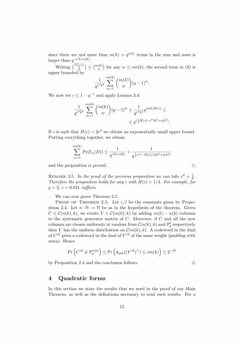
If c is such that H(c) < 2c′′ we obtain an exponentially small upper bound.Putting everything together, we obtain

cm(k)∑w=1

Pr(Ew(D)) ≤ 1

qc′k+o(k)+

1

q12(c′′−H(c)/2)k2+o(k2)

and the proposition is proved. 4

Remark 3.5. In the proof of the previous proposition we can take c′′ = 18 .

Therefore the proposition holds for any c with H(c) < 1/4. For example, forq = 2, c = 0.041 suffices.

We can now prove Theorem 2.5.Proof of Theorem 2.5. Let c, c be the constants given by Propo-

sition 2.4. Let n : N → N be as in the hypothesis of the theorem. GivenC ∈ C(n(k), k), we create V ∈ C(m(k), k) by adding m(k) − n(k) columnsto the systematic generator matrix of C. Moreover, if C and all the newcolumns are chosen uniformly at random from C(n(k), k) and Fkq respectivelythen V has the uniform distribution on C(m(k), k). A codeword in the dualof C∗2 gives a codeword in the dual of V ∗2 of the same weight (padding withzeros). Hence

Pr(C∗2 6= Fn(k)q

)≤ Pr

(dmin((V ∗2)

⊥) ≤ cm(k)

)≤ 2−ck

by Proposition 2.4 and the conclusion follows. 4

4 Quadratic forms

In this section we state the results that we need in the proof of our MainTheorem, as well as the definitions necessary to read such results. For a

12

more involved discussion, see Appendix A, where we include full proofs ofthe results stated here as well. Even though these can be found, at leastpartly, in the literature, we have felt it necessary to derive what we need ina unified way.

Throughout this section, let K be an arbitrary field.

Definition 4.1 (quadratic form). Let V be a finite dimensional K-vectorspace. A quadratic form on V is a map Q : V → K such that

(i) Q(λx) = λ2Q(x) for all x ∈ V, λ ∈ K,

(ii) the map (x, y) 7→ Q(x+ y)−Q(x)−Q(y) is a bilinear form on V .

The K-vector space of all quadratic forms on V is denoted by Quad(V ).A pair (V,Q) where V is a finite dimensional K-vector space and Q is aquadratic form on V is called a K-quadratic space.

Let (V,Q) be a K-quadratic space. With abuse of terminology, fromhere on we call V a quadratic space, omitting the quadratic form Q whichdefines the quadratic space structure on the vector space V . We define asymmetric bilinear form BQ on V by

BQ(x, y) := Q(x+ y)−Q(x)−Q(y)

for all x, y ∈ V .

Definition 4.2 (radical). The radical of the quadratic space V is the K-vector space

RadV := {x ∈ V : BQ(x, y) = 0 for all y ∈ V }.

We say that V is non-degenerate (as a quadratic space) if BQ is non-degenerate (as a bilinear form), i.e. if RadV = 0.

Definition 4.3 (rank). Let Rad0 V := {x ∈ RadV : Q(x) = 0}. We definethe rank of Q to be

rkQ := dimV − dim Rad0 V.

Remark 4.4. Note that in the case charK 6= 2, it holds that Q(x) =12BQ(x, x) and therefore Rad0 V = RadV . Hence in this case (V,Q) isnon-degenerate if and only if Q has full rank. In the appendix we show thatthis is not the case if charK = 2.

We are now ready to state the results we need. Theorem 4.5 counts thenumber of zeros of a given quadratic form. Theorem 4.6 counts the numberof quadratic forms of a given rank.

13

Theorem 4.5. Let (V,Q) be an Fq-quadratic space, set k := dimV andr := rkQ. The number of vectors x ∈ V such that Q(x) = 0 is

a. qk−1 if r is odd,

b. either qk−1 − (q − 1)qk−r2−1 or qk−1 + (q − 1)qk−

r2−1 if r is even.

Theorem 4.6. For all non-negative integers k, the number of full-rankquadratic forms on an Fq-vector space of dimension k is

N(k) = qbk2c(b k2c+1)

d k2e∏i=1

(q2i−1 − 1) =

=

qk−12

k+12∏ k+1

2i=1 (q2i−1 − 1) if k is odd,

qk2 ( k2+1)∏ k

2i=1(q

2i−1 − 1) if k is even.

For all non-negative integers k ≥ r, the number of rank r quadratic formson an Fq-vector space of dimension k is

N(k, r) =

[k

r

]N(r),

where[kr

]denotes the q-ary Gaussian binomial coefficient (see Definition 3.1).

A more general result implying Theorem 4.5 appears in [25, Chapter 6,Section 2].

As to Theorem 4.6, the following references need to be mentioned. In[2, Lemma 9.5.9] the number of symmetric bilinear forms of given rankis computed. In the odd characteristic case, as symmetric bilinear formscorrespond to quadratic forms and the two notions of rank coincide, thisresult is equivalent to Theorem 4.6. As to the arbitrary characteristic case,[2] refers to [18]. The latter uses the language of association schemes andgives a result that allows to compute (even though this is not explicitlystated) the number N ′(k, s) of quadratic forms of rank r ∈ {2s − 1, 2s} onan Fq-vector space of dimension k. This result is slightly weaker than ourtheorem, as it allows to compute the sum N(k, 2s− 1) +N(k, 2s) instead ofN(k, 2s− 1) and N(k, 2s) separately, but it would be sufficient for the mainpurpose of this work.

5 Proof of Main Theorem 2.2

We recall the notation introduced in Section 2. Given an [n, k]-code C anddenoting by π1, . . . , πn ∈ Fkq the columns of a generator matrix of C (i.e. amatrix whose rows form a basis of C), we define the linear map

evC : Quad(Fkq ) → Fnq ,Q 7→ (Q(π1), . . . , Q(πn))

14

whose image is C∗2.Recall that we have defined the random variable X(n, k) := | ker evC |,

with distribution induced by a uniform random selection of C from C(n, k).For simplicity, we will write Xk as a shorthand for X(k(k + 1)/2, k).

It is convenient to measure “how far” C∗2 is from being the full spaceby defining, for all positive integers n ≥ k and all non-negative integers `,the probabilities:

p`(n, k) := Pr(codimC∗2 ≤ `),

where C is chosen uniformly at random from C(n, k). Using this notation,Main Theorem 2.2 claims that there exists δ ∈ R>0 such that, for all largeenough k, p0(n(k), k) ≥ 1− 2−δt(k).

As mentioned before, crucial to the proof of Main Theorem 2.2 is toestimate the expected value of Xk = X(k(k + 1)/2, k): this is preciselythe purpose of Theorem 2.6, that states that limk→∞ E [Xk] = 2. We nowproceed to its proof.

Proof of Theorem 2.6. In Section 2 we defined the space S of allquadratic forms vanishing at all unit vectors and we proved that, for allpositive integers m ≥ k,

E[X(m, k)] =∑Q∈S

(|Z(Q)|qk

)m−k. (1)

We now fix a rank threshold, i.e. a fraction of k, and we classify theforms in S accordingly. Precisely, for any 0 < α < 1 we define

S−(α) := {Q ∈ S : 0 < rkQ ≤ αk},S+(α) := {Q ∈ S : rkQ > αk},

so S = {0} ∪ S+(α) ∪ S−(α). We observe that

|S−(α)| ≤ q(−α2

2+α)k2+o(k2). (4)

Indeed, by Theorem 4.6 we have

|S−(α)| =αk∑r=1

N(k, r) =αk∑r=1

[k

r

]N(r).

We loosely bound[kr

]≤ qr(k−r+1) and N(r) ≤ |Quad(Frq)| = qr(r+1)/2 and

we obtain

|S−(α)| ≤αk∑r=1

qr(k−r+1)qr(r+1)/2 =αk∑r=1

q−r2

2+(k+ 3

2)r ≤

≤ αkq(−α2

2+α)k2+ 3

2αk,

15

proving (4). This yields

|S−(α)||S|

≤ q(−α2

2+α)k2+o(k2)

qk(k−1)

2

= q−12(α−1)2k2+o(k2)

which tends to 0 as k →∞. Hence, noting that |S+(α)| = |S|−1−|S−(α)|,we obtain

limk→∞

|S+(α)||S|

= 1. (5)

In view to using the observations (4) and (5) on the “density” of S+(α) andS−(α) in S, we apply the partition of S to (1) and write

E[X(m, k)] =

= 1 +∑

Q∈S+(α)

(|Z(Q)|qk

)m−k+

∑Q∈S−(α)

(|Z(Q)|qk

)m−k. (6)

We now prove that the first sum tends to 1 while the second one (for somesuitable value of α) tends to 0.

By Theorem 4.5, the number of zeros of any form Q ∈ S+(α) is boundedby

|Z(Q)| ≤ qk−1 + (q − 1)qk−αk2−1 ≤ qk−1

(1 +

1

qαk2−1

)and

|Z(Q)| ≥ qk−1 − (q − 1)qk−αk2−1 ≥ qk−1

(1− 1

qαk2−1

).

It follows that

1

q

(1− 1

qαk2−1

)≤ |Z(Q)|

qk≤ 1

q

(1 +

1

qαk2−1

)hence (

1− 1

qαk2−1

)m−k|S+(α)|qm−k

≤∑

Q∈S+(α)

(|Z(Q)|qk

)m−k≤

≤

(1 +

1

qαk2−1

)m−k|S+(α)|qm−k

.

Setting m = k(k + 1)/2, we get(1− 1

qαk2−1

) k(k−1)2 |S+(α)|

|S|≤

∑Q∈S+(α)

(|Z(Q)|qk

) k(k−1)2

≤

≤

(1 +

1

qαk2−1

) k(k−1)2 |S+(α)|

|S|.

16

So the first sum in (6) is bounded, from above and from below, by functionswhich tend to 1 (by (5)), hence it tends to 1, too.

We now prove that if we take any 0 < α < 1 −√

logq(2q − 1)− 1, the

last sum in (6) tends to 0, which will conclude the proof of the theorem.By Theorem 4.5, all forms Q ∈ S−(α) satisfy

|Z(Q)| ≤ qk−1 + (q − 1)qk−2 = 2qk−1 − qk−2.

This is trivial for odd rank forms, as they always have exactly qk−1 zeros.We get ∑

Q∈S−(α)

(|Z(Q)|qk

)m−k≤(

2q − 1

q2

)m−k|S−(α)|.

Setting m = k(k + 1)/2 and using (4) we finally obtain∑Q∈S−(α)

(|Z(Q)|qk

)m−k≤

≤(

2q − 1

q2

) k(k−1)2

q(−α2

2+α)k2+o(k2) = qµ(α)k

2+o(k2),

where µ(α) := −12(α2−2α+ 2− logq(2q−1)) < 0 under the assumptions on

α. Therefore the right hand side tends to 0. This concludes the proof. 4As a first consequence of Theorem 2.6, we derive a proof of Theorem 2.3.Proof of Theorem 2.3. As before, set m(k) := k(k + 1)/2. Given a

code C ∈ C(n(k), k), we obtain a code C ′ ∈ C(m(k), k) puncturing the lasts(k) coordinates of C. We define N to be the event “dimC∗2 = m(k)” and,for all j ∈ N, we define Ej to be the event “| ker evC′ | = j”. We observe thatdimC∗2 = m(k) if and only if ker evC = 0, and this holds if and only if for allnonzero Q ∈ ker evC′ there exists i ∈ {m(k)+1, . . . , n(k)} such that Q(πi) 6=0. Hence, if in the case of Ej we write ker evC′ \{0} = {Q1, . . . , Qj−1}, wehave

Pr(N|Ej) =

= Pr

(j−1⋃i=1

{Qi(πm(k)+1) = · · · = Qi(πn(k)) = 0

})≤

≤j−1∑i=1

Pr(Qi(π) = 0)s(k),

for all j ∈ N, where π ∈ Fkq is chosen uniformly at random. Moreover, for

any nonzero quadratic form Q ∈ Quad(Fkq ),

Pr(Q(π) = 0) ≤ qk−1 + (q − 1)qk−2

qk=

2q − 1

q2.

17

Note that (2q − 1)/q2 is a constant strictly smaller than 1. It follows that

Pr(N|Ej) ≤j−1∑i=1

(2q − 1

q2

)s(k)= (j − 1)

(2q − 1

q2

)s(k).

Applying the law of total probability to Pr(N ) together with the aboveobservations we finally have

Pr(N ) =∑j∈N

Pr(Ej) Pr(N|Ej) ≤

≤(

2q − 1

q2

)s(k)∑j∈N

Pr(Ej)(j − 1) =

=

(2q − 1

q2

)s(k)(E[Xk]− 1).

The conclusion follows by Theorem 2.6. 4Next, we derive from the estimation of the expectation of Xk given by

Theorem 2.6, a lower bound for the probability of Xk being smaller thansome fixed constant. Precisely, the following holds.

Proposition 5.1. For any ε > 0 there exists kε ∈ N such that, for allk ≥ kε, for every non-negative integer ` we have

Pr

(dimC∗2 ≥ k(k + 1)

2− `)≥ 1− 2 + ε

q`+1,

where C is chosen uniformly at random from C(k(k + 1)/2, k).

Proof. We apply Markov’s inequality to the random variable Xk,namely:

Pr(Xk < δ) ≥ 1− E[Xk]

δ(7)

for any δ > 0. By Theorem 2.6 there exists kε ∈ N such that, for all k ≥ kε,we have E [Xk] ≤ 2 + ε, hence for any δ > 0, (7) gives

Pr(Xk < δ) ≥ 1− 2 + ε

δ

if k ≥ kε. Now setting δ = q`+1 and noting that Pr(Xk < q`+1) =Pr(dimC∗2 ≥ k(k + 1)/2− `) we conclude. 4

Proposition 5.1 together with Proposition 2.4 allow us to conclude theproof of Main Theorem 2.2.

Proof of Main Theorem 2.2. Let k ≤ n < m := k(k + 1)/2 bepositive integers, and let t := m − n. We use a puncturing argument.

18

The key observation is that a random code of length n can be obtained byfirst choosing a random code of length m and then deleting m− n randomcoordinates. We shall look closely at the probability that non-zero wordssurvive in the dual of the punctured code.

Precisely, consider a uniform random code C ∈ C(m, k): let C ′ ∈ C(n, k)be obtained from C by removing t random coordinates among the last m−k.Let these t coordinates be chosen uniformly, independently of C.

In order to estimate p0(n, k), we define the following events. Call E theevent studied in Proposition 2.4, namely dmin((C∗2)⊥) ≤ cm where c is theconstant of Proposition 2.4. For all non-negative integers i, call Ei the eventcodimC∗2 = i. As before, bar denotes the complement event.

For any positive integer ` we have

p0(n, k) ≥∑i=1

Pr(E ∩ Ei) Pr(codim(C ′)∗2 = 0|E ∩ Ei). (8)

Let C0 be a fixed code of length m and suppose x is a codeword of C⊥0 ofweight w. Puncture C0 by removing t random coordinates among the lastm−k. The probability that none of the random t coordinates belong to thesupport of x is at most (

m−wt

)(m−kt

) (9)

(and actually equal to (9) if the support of x contains the first k coordinates).If the dual code C⊥0 contains exactly qi− 1 non-zero codewords all of whichhave weight at least cm, then the probability that the t random coordinatesmiss the support of at least one codeword of C⊥0 is, by (9) and the unionbound, bounded from above by

(qi − 1)

(m−cm

t

)(m−kt

) .Now observing that a non-zero codeword in ((C ′)∗2)⊥ exists only if thereexists a non-zero codeword in (C∗2)⊥ with support disjoint from the chosent coordinates, we obtain that, for all i = 1, . . . , `,

Pr(codim(C ′)∗2 6= 0|E ∩ Ei) ≤ (qi − 1)

(m−cm

t

)(m−kt

) ≤≤ q`

(m−cm

t

)(m−kt

) .

19

We bound the fraction as follows:(m−cm

t

)(m−kt

) =(m− cm) · · · (m− cm− t+ 1)

(m− k) · · · (m− k − t+ 1)≤

≤(m− cmm− k

)t= (1− c)t

(k + 1

k − 1

)tfrom which we obtain

Pr(codim(C ′)∗2 6= 0|E ∩ Ei) ≤ q`+t(log(1−c)+log k+1k−1

).

Since log k+1k−1 goes to zero when k goes to infinity and log(1− c) is negative,

by fixing ` = αt we get the existence of a positive β such that, for any klarge enough,

Pr(codim(C ′)∗2 6= 0|E ∩ Ei) ≤ q−βt. (10)

Now note that by the union bound

Pr(E ∩ Ei) = 1− Pr(E ∪ E i) ≥ 1− Pr(E)− Pr(E i) =

= Pr(Ei)− Pr(E).

Therefore, (10) with (8) give

p0(n, k) ≥ (1− q−βt)∑i=1

(Pr(Ei)− Pr(E))

≥ (1− q−βt)(1− Pr(dimC∗2 ≤ m− `)− `Pr(E)). (11)

Proposition 5.1 gives us, since ` = αt, that Pr(dimC∗2 ≤ m − `) ≤ 2β′t for

a constant β′. Proposition 2.4 gives us, since ` ≤ k2, that `Pr(E) ≤ 2−γk

for some constant γ. From (11) we therefore get

p0(n, k) ≥ 1− 2−γk − 2−δt.

for constants γ and δ. 4

6 Changing the probabilistic model

In this section we expand Remark 2.1, with the purpose of showing that,even though our probabilistic model may appear restrictive, our analysisgives all the ingredients necessary to consider different models.

For all positive integers n ≥ k we define the following two families ofcodes. Let A(n, k) be the family of all codes of length n and dimension atmost k with the following distribution: choose a k × n matrix A uniformlyat random and pick the code spanned by the rows of A. Let U(n, k) be thefamily of all codes of length n and dimension k, with uniform distribution.

20

Note that it is equivalent to a uniform random choice of a k × n full-rankmatrix, as each such a code has the same number of bases, hence the samenumber of generator matrices.

We first argue that all our results hold if we replace C(n, k) with A(n, k).The two probability distributions are subtly different and it is not easy toderive results for A(n, k) from the results for C(n, k) seen as “black boxes”.However, if we go over the proofs of our theorems, we see that they willcarry over to A(n, k) with no significant change of strategy. Specifically,in the proof of Theorem 2.6, one will replace the study of the quantity∑

Q∈S

(|Z(Q)|qk

)m−kin (1) by

∑Q

(|Z(Q)|qk

)mwhere Q ranges over all quadratic forms on k variables. The quantity tobe studied is simply the expected number of quadratic forms that vanishon m random values. Going over the proof one will end up with exactlythe same expected value. We sum over a space with qk more quadraticforms but replace probabilities of the form (|Z(Q)|/qk)m−k by (|Z(Q)|/qk)mwhich behaves like 1/qk times less. Regarding the probabilistic analysisthat proves Proposition 2.4, we see that it is virtually unchanged when thefirst k coordinates become random. Also the puncturing argument thatproves Theorem 2.2 sees only the punctured coordinates being chosen from{1, . . . ,m} rather than from {k + 1, . . . ,m}.

Regarding the second distribution U(n, k), we argue differently and relateit to A(n, k). From here on n and k will be suppressed from the notation,since they are assumed to be fixed. We add indices as C ← A or C ← U toour probability notation to make the probabilistic model explicit. Observethat for any fixed code C0 of dimension k, we have

PrC←A

(C = C0|dimC = k) = PrC←U

(C = C0).

It follows that, if P(C) denotes a property that a code C may have,

PrD←U

(P(D)) = PrC←A

(P(C)| dimC = k).

We deduce from this observation that:

Lemma 6.1. For any property P,

PrD←U

(P(D)) ≥ PrC←A

(P(C))− PrC←A

(dimC < k).

21

Proof. We have

PrC←A

(P(C)) = PrC←A

(P(C)|dimC = k) PrC←A

(dimC = k)+

+ PrC←A

(P(C)|dimC < k) PrC←A

(dimC < k) ≤

≤ PrD←U

(P(D)) + PrC←A

(dimC < k).

4Next, recall this well-known result on random matrices:

PrC←A

(dimC < k) ≤ 1

qn−k.

Together with Lemma 6.1 this gives us:

PrD←U

(P(D)) ≥ PrC←A

(P(C))− 1

qn−k.

We can now apply this to versions of our Theorems forA(n, k). In particular,our main Theorem 2.2 will read, under the uniform distribution U(n, k), thatthere exist some positive real constants γ, δ such that

PrC←U

(C∗2 = Fn(k)q ) ≥ 1− 2−γk − 2−δt(k) − 1

qn(k)−k.

This simple argument is enough to recover an asymptotically optimal versionof our main result for the uniform distribution, except for code rates thattend to 1.

A Quadratic forms

This appendix is meant to be a continuation of Section 4. In particular, werefer to that section for the definitions of quadratic form, radical and rank.

Let K be a field, let (V,Q) be a K-quadratic space.With abuse of terminology, V itself is called a quadratic space. Recall

that V , as a vector space, is finite dimensional by definition. Any sub-space W of V inherits a natural structure of quadratic space, defined by therestriction of Q to W .

Recall that we defined a symmetric bilinear form BQ on V by

BQ(x, y) := Q(x+ y)−Q(x)−Q(y)

for all x, y ∈ V . If charK 6= 2 we also define the symmetric bilinear formBQ := 1

2BQ, which satisfies BQ(x, x) = Q(x) for all x ∈ V . If charK = 2

note that BQ is alternating, i.e. BQ(x, x) = 0 for all x ∈ V . As a shorthand,if there is no ambiguity we write x · y instead of BQ(x, y) for x, y ∈ V .

22

A remark concerning the definitions of radical and rank follows. IfcharK 6= 2 then Q vanishes on RadV : indeed, for all x ∈ RadV we haveQ(x) = BQ(x, x) = 1

2x · x = 0 by definition of the radical. If charK = 2this is not always the case: for example, consider the quadratic form on F2

defined by Q(x) := x2; note that BQ is identically zero, hence the radical isthe whole space, but Q does not vanish at x = 1. So in the characteristic 2case Rad0 V , the zero locus of the restriction of Q to RadV , is not neces-sarily trivial. Following [16], we have defined the rank of a quadratic formto be the codimension of this zero locus.

In the characteristic 2 case, under the additional assumption that K isperfect, i.e. squaring is an automorphism of K (which is always the case ifK is a finite field), one can prove that the difference between the rank of Qand the codimension of the radical of V is either zero or one.

We define orthogonality and isotropy with respect to BQ, as follows.Two vectors x, y ∈ V are orthogonal if x ·y = 0. Two subspaces V1, V2 ⊆

V are orthogonal if x · y = 0 for all x ∈ V1, y ∈ V2. We use the symbol ⊥ forthe orthogonality relation. The orthogonal of a subspace V1 ⊆ V is

V ⊥1 := {x ∈ V : x · y = 0 for all y ∈ V1}.

Note that V1 ∩V ⊥1 = RadV1, so RadV1 = 0 implies V1 ∩V ⊥1 = 0. Moreover,by basic linear algebra dimV1 + dimV ⊥1 = dimV . Hence in this case V ⊥1is a complement of V1, called the orthogonal complement of V1. Finally, adecomposition of V is orthogonal if the components are pairwise orthogonal.

A non-zero vector x ∈ V is isotropic if x · x = 0. A subspace of V isisotropic if it contains an isotropic vector, anisotropic otherwise. Note thatif charK = 2 then every vector is isotropic, as BQ is alternating, hence itdoes not make sense to use this notion.

A quadratic space (V,Q) is classified according to the orthogonal decom-position induced on V by Q. The “building blocks” in this decompositionare hyperbolic and symplectic planes, that are defined below.

Definition A.1 (hyperbolic plane). Assume that charK 6= 2. A hyperbolicplane is a non-degenerate 2-dimensional subspace which admits a basis ofisotropic vectors.

Note that any hyperbolic plane H admits a basis {v1, v2} of isotropicvectors such that v1 · v2 = 1. Indeed, for any basis {v1, w}, with v1, wisotropic, it holds that α := v1 · w 6= 0 as H is non-degenerate, hence{v1, v2} with v2 := α−1w satisfies the property.

Theorem A.2 (Witt’s decomposition). Assume that charK 6= 2. Then thequadratic space V orthogonally decomposes as

V = RadV ⊕m⊕i=1

Hi ⊕W,

23

where the Hi’s are hyperbolic planes and W is anisotropic. Moreover, if Kis finite then dimW ≤ 2.

Proof. Any complement of RadV is non-degenerate and orthogonal toRadV , so we may assume that RadV = 0, i.e. V is non-degenerate. If V isanisotropic we are done, with m = 0 and V = W . Otherwise there existsan isotropic vector v1 ∈ V , hence x ∈ V such that α := v1 · x 6= 0, as V isnon-degenerate. Now take

v2 :=1

αx− x · x

2α2v1,

H1 := 〈v1, v2〉 and apply induction.If K is finite then dimW ≤ 2, as any quadratic form on a non-degenerate

space of dimension larger than 2 has a non trivial zero, which is an isotropicvector of V . This is a consequence of the Chevalley-Warning Theorem, seefor example [32]. 4

Definition A.3 (symplectic plane). Assume that charK = 2. A symplecticplane is a subspace which admits a basis {v1, v2} such that v1 · v2 = 1.

Non-degeneracy is implied by this definition.

Theorem A.4. Assume that charK = 2. Then the quadratic space V or-thogonally decomposes as

V = RadV ⊕m⊕i=1

Si,

where the Si’s are symplectic planes. Moreover, all but at most one amongthe Si’s admit a K-basis {v1, v2} such that v1·v2 = 1 and Q(v1) = Q(v2) = 0.

Proof. Again, we may assume that V is non-degenerate. Let v1 ∈ V ,let x ∈ V be such that α := v1 · x 6= 0. Take v2 := 1

αx, S1 := 〈v1, v2〉and argue by induction. For the last statement, see [17] or [16, Chapter I,Section 16]. 4

Remark A.5. Stronger results actually hold. The decompositions above are,in some sense, unique: for example, in a Witt decomposition, the numberm of hyperbolic planes is unique while the anisotropic space W is unique upto “isometry”. For details, see [24, 32] for Theorem A.2 and [17, 16] forTheorem A.4. However, these stronger results are not needed here.

A.1 Number of zeros of a quadratic form

Let (V,Q) be a quadratic space over the finite field Fq.

24

In this section we compute the number of zeros in V of the quadratic formQ, as a function of the dimension k of V , the rank r ofQ and the cardinality qof the base field. Even though the definition of rank is essentially dependenton charFq, the formula we give is characteristic-free.

Theorem A.6. The number of vectors x ∈ V such that Q(x) = 0 is

a. qk−1 if r is odd,

b. either qk−1 − (q − 1)qk−r2−1 or qk−1 + (q − 1)qk−

r2−1 if r is even.

Remark A.7. The “±” in claim b of Theorem A.6 (and of the forthcom-ing Theorem A.9) only depends on the “last component” in the orthogonaldecomposition of V given by Theorem A.2 or Theorem A.4.

In [25, Chapter 6, Section 2] the number of vectors x ∈ V such thatQ(x) = b, for any full-rank quadratic form Q on V and any b ∈ Fq, iscomputed. Theorem A.9 below, whence Theorem A.6 easily follows, is aninstance of this result. However, for completeness, and to show an applica-tion of the classification theorems, we include a full proof of Theorem A.9.

Here, it is convenient to view quadratic forms as polynomials, as follows.This correspondence holds over an arbitrary field K (so we abandon fora moment the assumption that the base field is finite). Fixing a K-basis{v1, . . . , vk} of V we can associate to Q a homogeneous quadratic k-variatepolynomial fQ ∈ K[X1, . . . , Xk] such that, for all (α1, . . . , αk) ∈ Kk,

Q(α1v1 + · · ·+ αkvk) = fQ(α1, . . . , αk),

namely

fQ :=∑

1≤i≤kQ(vi)X

2i +

∑1≤i<j≤k

BQ(vi, vj)XiXj .

Clearly there is a one-to-one correspondence between zeros of Q and zerosof fQ, independently of the basis choice. We remark that the rank of Q canbe equivalently defined as the minimal number of variables appearing in thepolynomial fQ associated to Q, where minimality is taken over all possiblebasis choices.

Back to the case of K = Fq, we have the following straightforward con-sequence of the classification theorems.

Corollary A.8. Assume that r ≥ 3. Then the polynomial fQ associatedto Q in some suitable basis can be written as

fQ = gQ +Xk−1Xk, with gQ ∈ Fq[X1, . . . , Xk−2].

Proof. As r ≥ 3, the classification theorems give an Fq-basis {v1, . . . , vk}of V such that BQ(vk−1, vk) = 1, Q(vk−1) = Q(vk) = 0 and 〈v1, . . . , vk−2〉 ⊥

25

〈vk−1, vk〉. The polynomial fQ associated to Q with respect to this basis hasthe desired form. 4

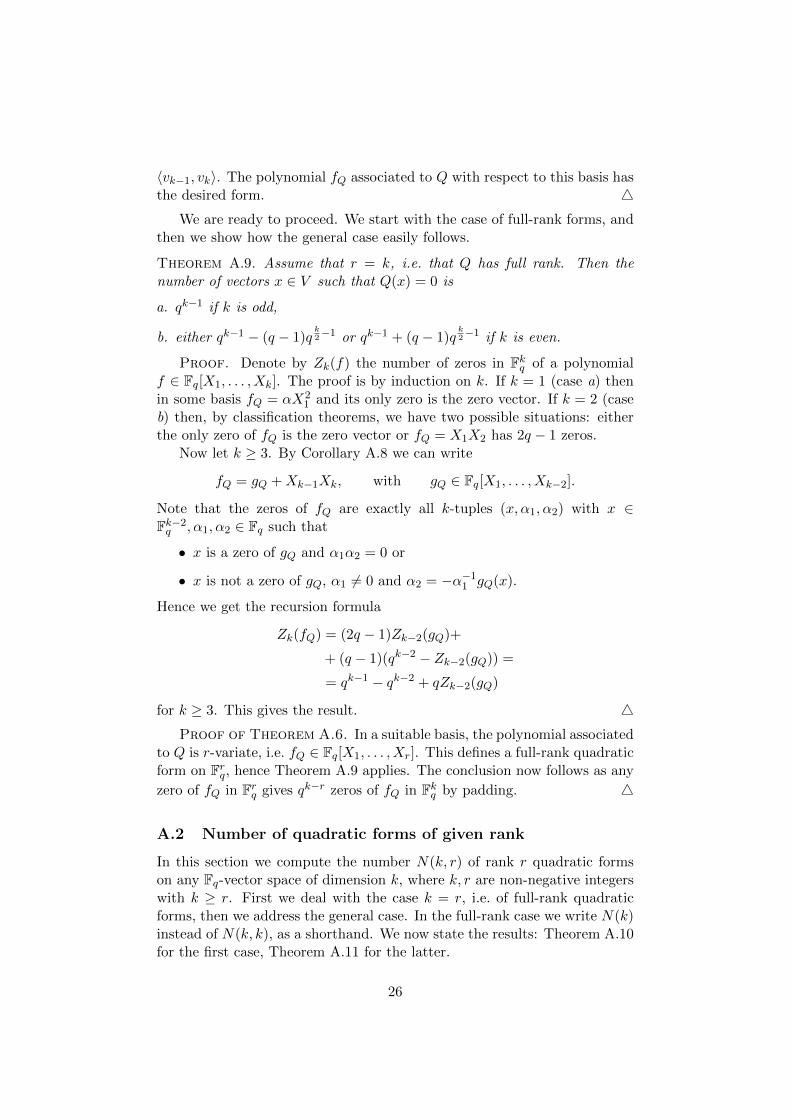
We are ready to proceed. We start with the case of full-rank forms, andthen we show how the general case easily follows.

Theorem A.9. Assume that r = k, i.e. that Q has full rank. Then thenumber of vectors x ∈ V such that Q(x) = 0 is

a. qk−1 if k is odd,

b. either qk−1 − (q − 1)qk2−1 or qk−1 + (q − 1)q

k2−1 if k is even.

Proof. Denote by Zk(f) the number of zeros in Fkq of a polynomialf ∈ Fq[X1, . . . , Xk]. The proof is by induction on k. If k = 1 (case a) thenin some basis fQ = αX2

1 and its only zero is the zero vector. If k = 2 (caseb) then, by classification theorems, we have two possible situations: eitherthe only zero of fQ is the zero vector or fQ = X1X2 has 2q − 1 zeros.

Now let k ≥ 3. By Corollary A.8 we can write

fQ = gQ +Xk−1Xk, with gQ ∈ Fq[X1, . . . , Xk−2].

Note that the zeros of fQ are exactly all k-tuples (x, α1, α2) with x ∈Fk−2q , α1, α2 ∈ Fq such that

• x is a zero of gQ and α1α2 = 0 or

• x is not a zero of gQ, α1 6= 0 and α2 = −α−11 gQ(x).

Hence we get the recursion formula

Zk(fQ) = (2q − 1)Zk−2(gQ)+

+ (q − 1)(qk−2 − Zk−2(gQ)) =

= qk−1 − qk−2 + qZk−2(gQ)

for k ≥ 3. This gives the result. 4Proof of Theorem A.6. In a suitable basis, the polynomial associated

to Q is r-variate, i.e. fQ ∈ Fq[X1, . . . , Xr]. This defines a full-rank quadraticform on Frq, hence Theorem A.9 applies. The conclusion now follows as any

zero of fQ in Frq gives qk−r zeros of fQ in Fkq by padding. 4

A.2 Number of quadratic forms of given rank

In this section we compute the number N(k, r) of rank r quadratic formson any Fq-vector space of dimension k, where k, r are non-negative integerswith k ≥ r. First we deal with the case k = r, i.e. of full-rank quadraticforms, then we address the general case. In the full-rank case we write N(k)instead of N(k, k), as a shorthand. We now state the results: Theorem A.10for the first case, Theorem A.11 for the latter.

26

Theorem A.10. For all non-negative integers k, the number of full-rankquadratic forms on an Fq-vector space of dimension k is

N(k) = qbk2c(b k2c+1)

d k2e∏i=1

(q2i−1 − 1) =

=

qk−12

k+12∏ k+1

2i=1 (q2i−1 − 1) if k is odd,

qk2 ( k2+1)∏ k

2i=1(q

2i−1 − 1) if k is even.

Theorem A.11. For all non-negative integers k ≥ r, the number of rank rquadratic forms on an Fq-vector space of dimension k is

N(k, r) =

[k

r

]N(r),

where[kr

]denotes the q-ary Gaussian binomial coefficient (see Definition 3.1).

Remark A.12. Recall that[kr

]equals the number of r-dimensional subspaces

of any Fq-vector space of dimension k.

Our proofs of Theorems A.10 and A.11 follow. Our strategy consists ofconstructing all quadratic forms on a given space as “combinations” (in thesense of Definition A.13 and Construction A.14 below) of quadratic forms onsubspaces. Counting recursively the number of forms constructed in this wayand dividing by the number of repetitions will give the required quantity.

Towards a proof of Theorem A.10, we fix a non-negative integer k andan Fq-vector space V of dimension k. We define the following “sum” ofquadratic forms.

Definition A.13. Let V1, V2 ≤ V be subspaces such that V1 ∩ V2 = 0, letQ1 be a quadratic form on V1 and Q2 a quadratic form on V2. We defineQ := Q1 ⊕ Q2 to be the unique quadratic form on V1 ⊕ V2 defined by theconditions Q|V1 = Q1, Q|V2 = Q2 and V1 ⊥ V2.

In other words, for v ∈ V1 ⊕ V2, we define Q(v) := Q1(v1) + Q2(v2),where v1 ∈ V1 and v2 ∈ V2 are the unique vectors such that v1 + v2 = v.Also note that Rad(V1 ⊕ V2) = RadV1 ⊕RadV2. So we construct quadraticforms on V as follows.

Construction A.14. Let h ≤ k be a non-negative integer. Let (V1, V2, Q1, Q2)be a 4-tuple consisting of a subspace V1 ≤ V of dimension h, a complementV2 ≤ V of V1, a full-rank quadratic form Q1 on V1 and a full-rank quadraticform Q2 on V2. Define Q := Q(V1,V2,Q1,Q2) := Q1 ⊕Q2 ∈ Quad(V ).

The choice of the parameter h is determined by the characteristic of Fqand the parity of the dimension k of V , as follows:

27

1. h = 1 if k is odd and charFq 6= 2,

2. h = 2 if k is even and charFq 6= 2,

3. h = 2 if charFq = 2.

We prove that, with this choice of h, all full-rank quadratic forms on Vare obtained by Construction A.14 and, conversely, all forms defined usingConstruction A.14 have full rank.

Lemma A.15. Any full-rank quadratic form on V is an instance of Con-struction A.14 with h chosen as above.

Proof. First assume that charFq 6= 2. If Q is a full-rank quadraticform on V then by Theorem A.2 we have an orthogonal decomposition

V =m⊕i=1

Hi ⊕W,

with dimHi = 2 for all i = 1, . . . ,m and dimW ≤ 2. If k is odd thendimW is also odd, hence it must equal 1. Let V1 := W , V2 :=

⊕mi=1Hi,

Q1 := Q|V1 and Q2 := Q|V2 , then Q = Q(V1,V2,Q1,Q2) with h = dimW = 1.If k is even, let V1 := H1, V2 :=

⊕mi=2Hi ⊕W,Q1 := Q|V1 , Q2 := Q|V2 , then

Q = Q(V1,V2,Q1,Q2) with h = dimH1 = 2.Now assume charFq = 2. If Q is a full-rank quadratic form on V then

by Theorem A.4 we have an orthogonal decomposition

V = RadV ⊕m⊕i=1

Si

with dim RadV = 0 or 1. Let V1 := S1, V2 := RadV ⊕⊕m

i=2 Si, Q1 :=Q|V1 , Q2 := Q|V2 , then Q = Q(V1,V2,Q1,Q2) with h = dimS1 = 2. 4

Lemma A.16. Any instance of Construction A.14, with h chosen as above,is a full-rank quadratic form on V .

Proof. Let V1, V2, Q1, Q2 be as in Construction A.14, and let Q :=Q(V1,V2,Q1,Q2). The statement is obvious if charFq is odd: in this case bothRadV1 = RadV2 = 0, hence Rad(V1 ⊕ V2) = 0 as well. The same happensin the characteristic 2 case if both h and k are even.

The only non trivial case is the one of charFq = 2 and k odd. We havechosen h to be even, hence RadV1 = 0 while RadV2 = 〈w〉 for some w ∈ V2such that Q(w) 6= 0. Then Rad(V1 ⊕ V2) = 〈w〉 and Q(w) = Q2(w) 6= 0,hence Q has full rank. 4

It follows that the number of full-rank quadratic forms on V is givenby the number of suitable 4-tuples (V1, V2, Q1, Q2) divided by the numberof repetitions. The number of possible choices for V1 is given by a Gaus-sian binomial coefficient. The following combinatorial lemma computes thenumber of possible choices for V2.

28

Lemma A.17. Let h ≤ k be a non-negative integer. The number of comple-ments of an h-dimensional subspace of V is qh(k−h).

Proof. LetW be an h-dimensional subspace of V , with basis {v1, . . . , vh}.This can be completed to a basis of V in (qk − qh)(qk − qh+1) · · · (qk − qk−1)ways. Any complement of W has dimension k− h, hence (qk−h− 1)(qk−h−q) · · · (qk−h − qk−h−1) different bases. Hence the number of complements ofW is

qk − qh

qk−h − 1· q

k − qh+1

qk−h − q· · · qk − qk−1

qk−h − qk−h−1= qh(k−h).

4Finally, we count how many times a quadratic form is repeated.

Lemma A.18. Let Q be a full-rank quadratic form on V . For any non-degenerate h-dimensional subspace V1 of V , with h chosen as above, wehave a unique complement V2 of V1 and unique full-rank quadratic forms Q1

and Q2 on V1 and V2 respectively such that Q = Q(V1,V2,Q1,Q2).

Proof. Let V1 be a non-degenerate h-dimensional subspace of V . Wewant to define V2, Q1, Q2 such that Q(V1,V2,Q1,Q2) = Q. Clearly we have totake Q1 := Q|V1 . The choice of h implies that RadV1 = 0, hence V1 has an

orthogonal complement. So take V2 := V ⊥1 and Q2 := Q|V2 . Note that theseare the only possible choices, hence this proves the lemma. 4

For all full-rank quadratic forms Q on V and all non-negative integers hwe denote byR(Q, h) the number of non-degenerate h-dimensional subspacesof V . A priori, this number depends on Q, but we will see that under ourchoice of h it only depends on k and h. In those cases we denote it byR(k, h).

All lemmas above together prove the following.

Lemma A.19. Let h be chosen as above, assume that R(k, h) = R(Q, h) isindependent of the choice of a quadratic form Q. Then

N(k) =

[kh

]qh(k−h)

R(k, h)N(h)N(k − h).

Remark A.20. By classification theorems, any quadratic form can be ob-tained by Construction A.14 with h = 2, independently of the rank parity.So it is natural to ask why, in the odd characteristic case, we are dealingseparately with odd rank and even rank quadratic forms, using h = 1 in thefirst case and h = 2 in the second. The reason is that if rkQ is odd thenR(Q, 2) depends on Q, yielding a formula more complicated than the onegiven by Lemma A.19, involving terms which also depend on Q. So ourstrategy allows a simpler proof.

29

Computing the number R(k, h) is the last non trivial step towards thecomputation of N(k). We are going to do that in the next two sections,obtaining the following recursion formula.

Theorem A.21. For k ≥ 1,

N(k) =

{(qk − 1)N(k − 1) if k is odd,

qkN(k − 1) if k is even.

Theorem A.21 will be proved in the next two sections, dealing with theodd characteristic case and with the characteristic 2 case separately. We nowuse it to prove the closed-form expression for N(k) stated by Theorem A.10.Then we will conclude this section with the proof of Theorem A.11.

Proof of Theorem A.10. We argue by induction on k. First note thatN(0) = 1 and N(1) = q − 1. Now let k > 1 and assume that the statementis true for k − 1. We use the recursion formula given by Theorem A.21. Ifk is odd then

N(k) = (qk − 1)N(k − 1) =

= (qk − 1)qk−12 ( k−1

2+1)

k−12∏i=1

(q2i−1 − 1) =

= qk−12

k+12

k+12∏i=1

(q2i−1 − 1).

If k is even then

N(k) = qkN(k − 1) =

= qkqk2 ( k2−1)

k2∏i=1

(q2i−1 − 1) =

= qk2 ( k2+1)

k2∏i=1

(q2i−1 − 1).

4Proof of Theorem A.11. Consider the following construction. For

any choice of a subspace V0 of dimension r, a full-rank quadratic form Q0

on V0 and a direct complement R of V0 we can define the quadratic formQ := Q(V0,Q0,R) := Q0 ⊕ 0 ∈ Quad(V ) of rank r, i.e. the unique quadraticform on V defined by the conditions Q|V0 = Q0, Q|R = 0 and V0 ⊥ R.By classification of quadratic forms, any rank r quadratic form is given byQ(V0,Q0,R) for some triple (V0, Q0, R).

30

So we only need to compute the number of times each form is repeated,i.e. the number of triples (V ′0 , Q

′0, R

′) such that Q(V ′0 ,Q′0,R′) = Q(V0,Q0,R) =:

Q, where (V0, Q0, R) is a fixed triple. First note that

R′ = {x ∈ RadV : Q(x) = 0} = R,

hence V ′0 has to be a direct complement of R. But for any direct complementV ′0 of R we have that the triple (V ′0 , Q|V ′0 , R) defines the form Q. So, for any

triple (V0, Q0, R), the number of triples (V ′0 , Q′0, R

′) such that Q(V ′0 ,Q′0,R′) =

Q(V0,Q0,R) is equal to the number of direct complements of R.

We are ready to conclude. We have[kr

]choices for V0, N(r) choices for

Q0 by definition, qr(k−r) choices for R by Lemma A.17 and any form occursqr(k−r) times. Hence N(k, r) =

[kr

]N(r), as claimed. 4

The next two sections constitute the proof of Theorem A.21. They sharea similar structure: first we compute R(k, h) in some interesting cases, thenwe use it, together with Lemma A.19, to prove Theorem A.21. Section A.2.1deals with the odd characteristic case, Section A.2.2 deals with the charac-teristic 2 case.

A.2.1 Odd characteristic case

In this section, assume that charFq is odd.

Lemma A.22. We have that

1. R(k, 1) = qk−1 if k is odd,

2. R(k, 2) = qk−2 qk−1q2−1 if k is even.

In particular, these numbers are independent of the choice of a full-rankquadratic form Q.

Proof. Let Q be a full-rank quadratic form on V . All 1-dimensionalsubspaces V1 ≤ V such that Q|V1 has full rank are given by V1 = 〈v1〉 for

some vector v1 ∈ V such that Q(v1) 6= 0. As Q has odd rank, it has qk−1

zeros, hence we have qk − qk−1 possible choices for v1. But 〈λv1〉 = 〈v1〉for any λ ∈ Fq, λ 6= 0, hence each subspace is counted q − 1 times. So

R(k, 1) = qk−qk−1

q−1 = qk−1, and this proves the first claim.We now prove the second claim. We can choose any non zero v1 ∈ V

as first basis vector of V1 and we want to count the number of vectorsv2 ∈ V \ 〈v〉 such that Q|〈v1,v2〉 has full rank. This holds if and only if

det

(BQ(v1, v1) BQ(v1, v2)

BQ(v1, v2) BQ(v2, v2)

)6= 0,

31

i.e. if and only if v2 is not a zero of the quadratic form on V defined by

Q′(x) := BQ(v1, v1)BQ(x, x)− BQ(v1, x)2

for x ∈ V . One can easily verify that this is indeed a quadratic form andthat the associated bilinear form is defined by

BQ′(x, y) = 2BQ(v1, v1)BQ(x, y)− 2BQ(v1, x)BQ(v1, y)

for x, y ∈ V . We distinguish two cases. If BQ(v1, v1) = 0 then Q′(x) =

−BQ(v1, x)2

is the square of a non zero linear form, hence it has rank 1. IfBQ(v1, v1) 6= 0 then the radical of V with respect to BQ′ is exactly the spanof v1, hence rkQ′ = rkQ− 1 is odd as rkQ is even. In order to prove this,let w ∈ RadV (with respect to BQ′), i.e. BQ′(w, y) = 0 for all y ∈ V . Then

BQ′(w, y) = 2BQ(v1, v1)BQ(w, y)− 2BQ(v1, w)BQ(v1, y) =

= 2BQ(BQ(v1, v1)w − BQ(v1, w)v1, y) = 0

for all y ∈ V . But BQ is non-degenerate, hence this implies that BQ(v1, v1)w =BQ(v1, w)v1, therefore w ∈ 〈v1〉 as BQ(v1, v1) 6= 0. This proves that RadV ⊆〈v1〉, and the converse inclusion is obvious. So in any case rkQ′ is odd, henceQ′ has qk−1 zeros. We can finally conclude. We have qk − 1 choices for v1and qk − qk−1 choices for v2, and any subspace is given by (q2 − 1)(q2 − q)different choices of v1, v2 (corresponding to the number of bases of 〈v1, v2〉).So we have R(k, 2) = (qk−1)(qk−qk−1)

(q2−1)(q2−q) = qk−2 qk−1q2−1 . This concludes the proof.

4The following theorem implies Theorem A.21 in the odd characteristic

case. First we need two remarks. Full-rank quadratic forms on Fq correspondto non zero elements of Fq, hence N(1) = q − 1. Full-rank quadratic formson F2

q correspond to triples (x, y, z) ⊆ F3q such that xy − z2 6= 0, which is a

quadratic form of rank 3, hence N(2) = q3 − q2 = q2(q − 1).

Theorem A.23. For k ≥ 1,

N(k) =

{(qk − 1)N(k − 1) if k is odd,

qk(qk−1 − 1)N(k − 2) if k is even.

Proof. If k is odd then we apply Construction A.14 with h = 1. ByLemma A.19 and the first claim of Lemma A.22 we have

N(k) =

[k1

]qk−1

R(k, 1)N(1)N(k − 1) =

=qk − 1

q − 1

qk−1

qk−1(q − 1)N(k − 1) =

= (qk − 1)N(k − 1).

32

If k is even then we apply Construction A.14 with h = 2. By Lemma A.19and the second claim of Lemma A.22 we have

N(k) =

[k2

]q2(k−2)

R(k, 2)N(2)N(k − 2) =

=(qk − 1)(qk−1 − 1)

(q2 − 1)(q − 1)q2(k−2)×

× 1

qk−2q2 − 1

qk − 1q2(q − 1)N(k − 2) =

= qk(qk−1 − 1)N(k − 2).

4

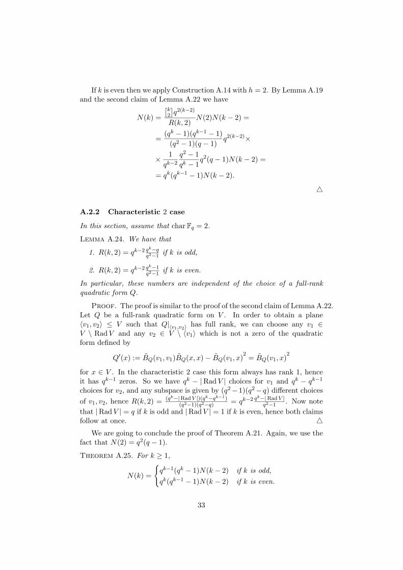
A.2.2 Characteristic 2 case

In this section, assume that charFq = 2.

Lemma A.24. We have that

1. R(k, 2) = qk−2 qk−qq2−1 if k is odd,

2. R(k, 2) = qk−2 qk−1q2−1 if k is even.

In particular, these numbers are independent of the choice of a full-rankquadratic form Q.

Proof. The proof is similar to the proof of the second claim of Lemma A.22.Let Q be a full-rank quadratic form on V . In order to obtain a plane〈v1, v2〉 ≤ V such that Q|〈v1,v2〉 has full rank, we can choose any v1 ∈V \ RadV and any v2 ∈ V \ 〈v1〉 which is not a zero of the quadraticform defined by

Q′(x) := BQ(v1, v1)BQ(x, x)− BQ(v1, x)2

= BQ(v1, x)2

for x ∈ V . In the characteristic 2 case this form always has rank 1, henceit has qk−1 zeros. So we have qk − |RadV | choices for v1 and qk − qk−1choices for v2, and any subspace is given by (q2−1)(q2− q) different choices

of v1, v2, hence R(k, 2) = (qk−|RadV |)(qk−qk−1)(q2−1)(q2−q) = qk−2 q

k−|RadV |q2−1 . Now note

that |RadV | = q if k is odd and |RadV | = 1 if k is even, hence both claimsfollow at once. 4

We are going to conclude the proof of Theorem A.21. Again, we use thefact that N(2) = q2(q − 1).

Theorem A.25. For k ≥ 1,

N(k) =

{qk−1(qk − 1)N(k − 2) if k is odd,

qk(qk−1 − 1)N(k − 2) if k is even.

33

Proof. Recall that in this case we use Construction A.14 with h = 2.By Lemma A.19 we have

N(k) =

[k2

]q2(k−2)

R(k, 2)N(2)N(k − 2) =

=1

R(k, 2)q2(k−2)q2(q − 1)×

× (qk − 1)(qk−1 − 1)

(q2 − 1)(q − 1)N(k − 2).

If k is odd then by claim 1 of Lemma A.24 we have

N(k) =q2 − 1

qk − q1

qk−2q2(k−2)q2(q − 1)×

× (qk − 1)(qk−1 − 1)

(q2 − 1)(q − 1)N(k − 2) =

= qk−1(qk − 1)N(k − 2).

If k is even then by claim 2 of Lemma A.24 we have

N(k) =q2 − 1

qk − 1

1

qk−2q2(k−2)q2(q − 1)×

× (qk − 1)(qk−1 − 1)

(q2 − 1)(q − 1)N(k − 2) =

= qk(qk−1 − 1)N(k − 2).

4

Acknowledgment

We wish to thank an anonymous reviewer for valuable comments that helpedsubstantially improve the paper.

References

[1] S. Ballet, J. Pieltant. On the tensor rank of multiplication in anyextension of F2. J. Complexity, Vol. 27, pp. 230-245, 2011.

[2] A. E. Brouwer, A. M. Cohen, A. Neumaier. Distance-Regular Graphs.Springer Verlag, 1989.

[3] I. Cascudo, H. Chen, R. Cramer, C. Xing. Asymptotically good ideallinear secret sharing with strong multiplication over any finite field.Proc. of 29th Annual IACR CRYPTO, Santa Barbara, Ca., USA,Springer Verlag LNCS, vol. 5677, pp. 466-486, August 2009.

34

[4] I. Cascudo, R. Cramer, C. Xing. The Torsion-Limit for Algebraic Func-tion Fields and Its Application to Arithmetic Secret Sharing. Proc. of31st Annual IACR CRYPTO, Santa Barbara, Ca., USA, Springer Ver-lag LNCS, vol. 6842, pp. 685-705, August 2011.

[5] I. Cascudo, R. Cramer, C. Xing. The Arithmetic Codex. IACR Cryptol-ogy ePrint Archive 2012: 388 (2012). A 5-page summary also appearedin Proceedings of IEEE Information Theory Workshop (ITW) 2012.

[6] I. Cascudo, R. Cramer, C. Xing. Torsion Limits and Riemann-RochSystems for Function Fields and Applications. IEEE Trans. Inform.Theory, Vol. 60, pp. 3871-3888, July 2014.

[7] I. Cascudo, R. Cramer, C. Xing, A. Yang. Asymptotic bound for multi-plication complexity in the extensions of small finite fields. IEEE Trans.Inform. Theory, Vol. 58, pp. 4930-4935, July 2012.

[8] H. Chen and R. Cramer. Algebraic Geometric Secret Sharing Schemesand Secure Multi-Party Computation over Small Fields. Proc. of 26thAnnual IACR CRYPTO, Springer Verlag LNCS, vol. 4117, pp. 516-531,Santa Barbara, Ca., USA, August 2006.

[9] H. Chen, R. Cramer, S. Goldwasser, R. de Haan, V. Vaikuntanathan.Secure Computation from Random Error Correcting Codes. Proc. of27th Annual IACR EUROCRYPT, Barcelona, Spain, Springer VerlagLNCS, vol. 4515, pp. 291-310, 2007.

[10] J. H. Conway, N. J. A. Sloane. Sphere packings, lattices and groups.Springer, 1999 (3rd Edition).

[11] A. Couvreur, P. Gaborit, V. Gauthier, A. Otmani, J.-P. Tillich.Distinguisher-based attacks on public-key cryptosystems using Reed-Solomon codes. Designs Codes and Cryptography, vol. 73, pp. 641-666,November 2014.

[12] A. Couvreur, A. Otmani, J.-P. Tillich. New Identities Relating WildGoppa Codes. Finite Fields Appl., vol. 29, pp. 178-197, 2014.

[13] A. Couvreur, A. Otmani, J.-P. Tillich. Polynomial Time Attack onWild McEliece Over Quadratic Extensions. Proceedings of 33rd AnnualIACR EUROCRYPT, Copenhagen, Denmark, Springer Verlag LNCS,vol. 8441, pp. 17-39, May 2014.

[14] R. Cramer, I. Damgard, U. Maurer. General secure multi-party compu-tation from any linear secret sharing scheme. Proceedings of 19th An-nual IACR EUROCRYPT, Brugge, Belgium, Springer Verlag LNCS,vol. 1807, pp. 316-334, May 2000.

35

[15] R. Cramer, I. Damgard, J. B. Nielsen. Secure Multiparty Computationand Secret Sharing. Cambridge University Press, to appear.

[16] J. Dieudonne. La Geometrie des Groupes Classiques, 2nd edition.Springer-Verlag, 1963.

[17] R. H. Dye. On the Arf Invariant. Journal of Algebra, pp. 36-39, 1978.

[18] Y. Egawa. Association Schemes of Quadratic Forms. Journal of Com-binatorial Theory, Series A 38, pp. 1-14, 1985.

[19] J.-C. Faugere, V. Gauthier-Umana, A. Otmani, L. Perret, J-P. Tillich,A distinguisher for high rate McEliece cryptosystems. Proceedings IEEEInformation Theory Workshop, Paraty, Brazil 2011.

[20] W. C. Huffman, V. Pless. Fundamentals of Error-Correcting Codes.Cambridge University Press, 2003.

[21] Y. Ishai, E. Kushilevitz, R. Ostrovsky, M. Prabhakaran, A. Sahai,J. Wullschleger. Constant-Rate Oblivious Transfer from Noisy Chan-nels. Crypto 2011, LNCS 6841, pp. 667-684, 2011.

[22] Y. Ishai, E. Kushilevitz, R. Ostrovsky, A. Sahai. Zero-knowledge proofsfrom secure multiparty computation. SIAM J. Comput., Vol. 39(3),pp. 1121-1152, 2009.

[23] W. Kositwattanarerk, F. Oggier. Connections Between Construction Dand Related Constructions of Lattices. Designs Codes and Cryptogra-phy, vol. 73,pp. 441-455, November 2014.

[24] T. Y. Lam. Introduction to Quadratic Forms over Fields. GraduateStudies in Mathematics 67, American Mathematical Society, 2005.

[25] R. Lidl, H. Niederreiter. Finite Fields. Addison-Wesley, 1983.

[26] F. J. McWilliams, N. J. A. Sloane. The Theory of Error-CorrectingCodes. North-Holland, 1977.

[27] F. Oggier, G. Zemor. Coding constructions for efficient oblivious trans-fer from noisy channels. Preprint.

[28] R. Pellikaan. On decoding by error location and dependent sets of errorpositions. Discrete Math., Vol. 106/107, pp. 369-381, 1992.

[29] H. Randriambololona. Bilinear complexity of algebras and theChudnovsky-Chudnovsky interpolation method. J. Complexity, Vol. 28,pp. 489-517, 2012.

36

[30] H. Randriambololona. Asymptotically good binary linear codes withasymptotically good self-intersection spans. IEEE Trans. Inform. The-ory, Vol. 59, pp. 3038-3045, May 2013.

[31] H. Randriambololona. On products and powers of lin-ear codes under componentwise multiplication. Preprint:http://arxiv.org/abs/1312.0022.

[32] J. -P. Serre. A Course in Arithmetic. Graduate Texts in Mathematics7, Springer, 1973.

37