SPSS Trends™ 14 - Kuwait University Trends 14.0.pdf · Training Seminars SPSS Inc. provides both...

SPSS Trends™ 14.0

For more information about SPSS® software products, please visit our Web site at http://www.spss.com or contact

SPSS Inc.

233 South Wacker Drive, 11th Floor

Chicago, IL 60606-6412

Tel: (312) 651-3000

Fax: (312) 651-3668

SPSS is a registered trademark and the other product names are the trademarks of SPSS Inc. for its proprietary computer software. No

material describing such software may be produced or distributed without the written permission of the owners of the trademark and

license rights in the software and the copyrights in the published materials.

The SOFTWARE and documentation are provided with RESTRICTED RIGHTS. Use, duplication, or disclosure by the Government is

subject to restrictions as set forth in subdivision (c) (1) (ii) of The Rights in Technical Data and Computer Software clause at 52.227-7013.

Contractor/manufacturer is SPSS Inc., 233 South Wacker Drive, 11th Floor, Chicago, IL 60606-6412.

General notice: Other product names mentioned herein are used for identification purposes only and may be trademarks of their

respective companies.

TableLook is a trademark of SPSS Inc.

Windows is a registered trademark of Microsoft Corporation.

DataDirect, DataDirect Connect, INTERSOLV, and SequeLink are registered trademarks of DataDirect Technologies.

Portions of this product were created using LEADTOOLS © 1991–2000, LEAD Technologies, Inc. ALL RIGHTS RESERVED.

LEAD, LEADTOOLS, and LEADVIEW are registered trademarks of LEAD Technologies, Inc.

Sax Basic is a trademark of Sax Software Corporation. Copyright © 1993–2004 by Polar Engineering and Consulting. All rights reserved.

Portions of this product were based on the work of the FreeType Team (http://www.freetype.org).

A portion of the SPSS software contains zlib technology. Copyright © 1995–2002 by Jean-loup Gailly and Mark Adler. The zlib

software is provided “as is,” without express or implied warranty.

A portion of the SPSS software contains Sun Java Runtime libraries. Copyright © 2003 by Sun Microsystems, Inc. All rights reserved.

The Sun Java Runtime libraries include code licensed from RSA Security, Inc. Some portions of the libraries are licensed from IBM and

are available at http://oss.software.ibm.com/icu4j/.

SPSS Trends™ 14.0

Copyright © 2005 by SPSS Inc.

All rights reserved.

Printed in the United States of America.

No part of this publication may be reproduced, stored in a retrieval system, or transmitted, in any form or by any means, electronic,

mechanical, photocopying, recording, or otherwise, without the prior written permission of the publisher.

1 2 3 4 5 6 7 8 9 0 08 07 06 05

ISBN 1-56827-373-8

Preface

SPSS 14.0 is a comprehensive system for analyzing data. The SPSS Trends optionaladd-on module provides the additional analytic techniques described in this manual.The Trends add-on module must be used with the SPSS 14.0 Base system and iscompletely integrated into that system.

Installation

To install the SPSS Trends add-on module, run the License Authorization Wizard usingthe authorization code that you received from SPSS Inc. For more information, see theinstallation instructions supplied with the SPSS Trends add-on module.

Compatibility

SPSS is designed to run on many computer systems. See the installation instructionsthat came with your system for specific information on minimum and recommendedrequirements.

Serial Numbers

Your serial number is your identification number with SPSS Inc. You will need thisserial number when you contact SPSS Inc. for information regarding support, payment,or an upgraded system. The serial number was provided with your Base system.

Customer Service

If you have any questions concerning your shipment or account, contact your localoffice, listed on the SPSS Web site at http://www.spss.com/worldwide. Please haveyour serial number ready for identification.

iii

Training Seminars

SPSS Inc. provides both public and onsite training seminars. All seminars featurehands-on workshops. Seminars will be offered in major cities on a regular basis. Formore information on these seminars, contact your local office, listed on the SPSS Website at http://www.spss.com/worldwide.

Technical Support

The services of SPSS Technical Support are available to maintenance customers.Customers may contact Technical Support for assistance in using SPSS or forinstallation help for one of the supported hardware environments. To reach TechnicalSupport, see the SPSS Web site at http://www.spss.com, or contact your local office,listed on the SPSS Web site at http://www.spss.com/worldwide. Be prepared to identifyyourself, your organization, and the serial number of your system.

Additional Publications

Additional copies of SPSS product manuals may be purchased directly from SPSS Inc.Visit the SPSS Web Store at http://www.spss.com/estore, or contact your local SPSSoffice, listed on the SPSS Web site at http://www.spss.com/worldwide. For telephoneorders in the United States and Canada, call SPSS Inc. at 800-543-2185. For telephoneorders outside of North America, contact your local office, listed on the SPSS Web site.

The SPSS Statistical Procedures Companion, by Marija Norušis, has been publishedby Prentice Hall. A new version of this book, updated for SPSS 14.0, is planned.The SPSS Advanced Statistical Procedures Companion, also based on SPSS 14.0, isforthcoming. The SPSS Guide to Data Analysis for SPSS 14.0 is also in development.Announcements of publications available exclusively through Prentice Hall will beavailable on the SPSS Web site at http://www.spss.com/estore (select your homecountry, and then click Books).

Tell Us Your Thoughts

Your comments are important. Please let us know about your experiences with SPSSproducts. We especially like to hear about new and interesting applications usingthe SPSS Trends add-on module. Please send e-mail to [email protected] or writeto SPSS Inc., Attn.: Director of Product Planning, 233 South Wacker Drive, 11thFloor, Chicago, IL 60606-6412.

iv

About This Manual

This manual documents the graphical user interface for the procedures included in theSPSS Trends add-on module. Illustrations of dialog boxes are taken from SPSS forWindows. Dialog boxes in other operating systems are similar. Detailed informationabout the command syntax for features in the SPSS Trends add-on module is availablein two forms: integrated into the overall Help system and as a separate document inPDF form in the SPSS 14.0 Command Syntax Reference, available from the Help menu.

Contacting SPSS

If you would like to be on our mailing list, contact one of our offices, listed on our Website at http://www.spss.com/worldwide.

v

Contents

Part I: User's Guide

1 Introduction to Time Series in SPSS 1

Time Series Data in SPSS . . . . . . . . . . . . . . . . . . . . . . . . . . . . . . . . . . . . . . . . 2Data Transformations . . . . . . . . . . . . . . . . . . . . . . . . . . . . . . . . . . . . . . . . . . . 2Estimation and Validation Periods . . . . . . . . . . . . . . . . . . . . . . . . . . . . . . . . . . 3Building Models and Producing Forecasts . . . . . . . . . . . . . . . . . . . . . . . . . . . 3

2 Time Series Modeler 5

Specifying Options for the Expert Modeler . . . . . . . . . . . . . . . . . . . . . . . . . . . 9Model Selection and Event Specification . . . . . . . . . . . . . . . . . . . . . . . . 10Handling Outliers with the Expert Modeler . . . . . . . . . . . . . . . . . . . . . . . 12

Custom Exponential Smoothing Models . . . . . . . . . . . . . . . . . . . . . . . . . . . . 13Custom ARIMA Models. . . . . . . . . . . . . . . . . . . . . . . . . . . . . . . . . . . . . . . . . 15

Model Specification for Custom ARIMA Models. . . . . . . . . . . . . . . . . . . 16Transfer Functions in Custom ARIMA Models . . . . . . . . . . . . . . . . . . . . 18Outliers in Custom ARIMA Models . . . . . . . . . . . . . . . . . . . . . . . . . . . . . 20

Output . . . . . . . . . . . . . . . . . . . . . . . . . . . . . . . . . . . . . . . . . . . . . . . . . . . . . 21Statistics and Forecast Tables . . . . . . . . . . . . . . . . . . . . . . . . . . . . . . . . 22Plots . . . . . . . . . . . . . . . . . . . . . . . . . . . . . . . . . . . . . . . . . . . . . . . . . . . 24Limiting Output to the Best- or Poorest-Fitting Models . . . . . . . . . . . . . . 26

Saving Model Predictions and Model Specifications. . . . . . . . . . . . . . . . . . . 28Options. . . . . . . . . . . . . . . . . . . . . . . . . . . . . . . . . . . . . . . . . . . . . . . . . . . . . 30TSMODEL Command Additional Features . . . . . . . . . . . . . . . . . . . . . . . . . . . 32

vii

3 Apply Time Series Models 33

Output . . . . . . . . . . . . . . . . . . . . . . . . . . . . . . . . . . . . . . . . . . . . . . . . . . . . . 37Statistics and Forecast Tables . . . . . . . . . . . . . . . . . . . . . . . . . . . . . . . . 38Plots . . . . . . . . . . . . . . . . . . . . . . . . . . . . . . . . . . . . . . . . . . . . . . . . . . . 41Limiting Output to the Best- or Poorest-Fitting Models . . . . . . . . . . . . . . 43

Saving Model Predictions and Model Specifications. . . . . . . . . . . . . . . . . . . 45Options. . . . . . . . . . . . . . . . . . . . . . . . . . . . . . . . . . . . . . . . . . . . . . . . . . . . . 47TSAPPLY Command Additional Features . . . . . . . . . . . . . . . . . . . . . . . . . . . . 48

4 Seasonal Decomposition 49

Seasonal Decomposition Save . . . . . . . . . . . . . . . . . . . . . . . . . . . . . . . . . . . 51SEASON Command Additional Features . . . . . . . . . . . . . . . . . . . . . . . . . . . . 52

5 Spectral Plots 53

SPECTRA Command Additional Features. . . . . . . . . . . . . . . . . . . . . . . . . . . . 56

Part II: Examples

6 Bulk Forecasting with the Expert Modeler 59

Examining Your Data . . . . . . . . . . . . . . . . . . . . . . . . . . . . . . . . . . . . . . . . . . . 59Running the Analysis . . . . . . . . . . . . . . . . . . . . . . . . . . . . . . . . . . . . . . . . . . 61Model Summary Charts . . . . . . . . . . . . . . . . . . . . . . . . . . . . . . . . . . . . . . . . 68

viii

Model Predictions . . . . . . . . . . . . . . . . . . . . . . . . . . . . . . . . . . . . . . . . . . . . 70Summary . . . . . . . . . . . . . . . . . . . . . . . . . . . . . . . . . . . . . . . . . . . . . . . . . . . 71

7 Bulk Reforecasting by Applying Saved Models 73

Running the Analysis . . . . . . . . . . . . . . . . . . . . . . . . . . . . . . . . . . . . . . . . . . 73Model Fit Statistics . . . . . . . . . . . . . . . . . . . . . . . . . . . . . . . . . . . . . . . . . . . . 78Model Predictions . . . . . . . . . . . . . . . . . . . . . . . . . . . . . . . . . . . . . . . . . . . . 79Summary . . . . . . . . . . . . . . . . . . . . . . . . . . . . . . . . . . . . . . . . . . . . . . . . . . . 79

8 Using the Expert Modeler to Determine SignificantPredictors 81

Plotting Your Data . . . . . . . . . . . . . . . . . . . . . . . . . . . . . . . . . . . . . . . . . . . . . 81Running the Analysis . . . . . . . . . . . . . . . . . . . . . . . . . . . . . . . . . . . . . . . . . . 84Series Plot . . . . . . . . . . . . . . . . . . . . . . . . . . . . . . . . . . . . . . . . . . . . . . . . . . 89Model Description Table . . . . . . . . . . . . . . . . . . . . . . . . . . . . . . . . . . . . . . . . 90Model Statistics Table . . . . . . . . . . . . . . . . . . . . . . . . . . . . . . . . . . . . . . . . . 90ARIMA Model Parameters Table. . . . . . . . . . . . . . . . . . . . . . . . . . . . . . . . . . 91Summary . . . . . . . . . . . . . . . . . . . . . . . . . . . . . . . . . . . . . . . . . . . . . . . . . . . 91

9 Experimenting with Predictors by Applying SavedModels 93

Extending the Predictor Series . . . . . . . . . . . . . . . . . . . . . . . . . . . . . . . . . . . 94Modifying Predictor Values in the Forecast Period . . . . . . . . . . . . . . . . . . . . 99Running the Analysis . . . . . . . . . . . . . . . . . . . . . . . . . . . . . . . . . . . . . . . . . 101

ix

10 Seasonal Decomposition 107

Removing Seasonality from Sales Data . . . . . . . . . . . . . . . . . . . . . . . . . . . . 107Preliminaries . . . . . . . . . . . . . . . . . . . . . . . . . . . . . . . . . . . . . . . . . . . . 107Determining and Setting the Periodicity . . . . . . . . . . . . . . . . . . . . . . . . 108Running the Analysis . . . . . . . . . . . . . . . . . . . . . . . . . . . . . . . . . . . . . . 113Understanding the Output . . . . . . . . . . . . . . . . . . . . . . . . . . . . . . . . . . 114Summary . . . . . . . . . . . . . . . . . . . . . . . . . . . . . . . . . . . . . . . . . . . . . . . 116

Related Procedures . . . . . . . . . . . . . . . . . . . . . . . . . . . . . . . . . . . . . . . . . . 117

11 Spectral Plots 119

Using Spectral Plots to Verify Expectations about Periodicity . . . . . . . . . . . 119Running the Analysis . . . . . . . . . . . . . . . . . . . . . . . . . . . . . . . . . . . . . . 119Understanding the Periodogram and Spectral Density . . . . . . . . . . . . . 121Summary . . . . . . . . . . . . . . . . . . . . . . . . . . . . . . . . . . . . . . . . . . . . . . . 124

Related Procedures . . . . . . . . . . . . . . . . . . . . . . . . . . . . . . . . . . . . . . . . . . 124

x

Appendices

A Goodness-of-Fit Measures 125

B Outlier Types 127

C Guide to ACF/PACF Plots 129

Bibliography 135

Index 137

xi

Part I:User's Guide

Chapter

1Introduction to Time Series inSPSS

A time series is a set of observations obtained by measuring a single variable regularlyover a period of time. In a series of inventory data, for example, the observations mightrepresent daily inventory levels for several months. A series showing the market shareof a product might consist of weekly market share taken over a few years. A series oftotal sales figures might consist of one observation per month for many years. Whateach of these examples has in common is that some variable was observed at regular,known intervals over a certain length of time. Thus, the form of the data for a typicaltime series is a single sequence or list of observations representing measurementstaken at regular intervals.

Table 1-1Daily inventory time series

Time Week Day Inventorylevel

t1 1 Monday 160

t2 1 Tuesday 135

t3 1 Wednesday 129

t4 1 Thursday 122

t5 1 Friday 108

t6 2 Monday 150

...

t60 12 Friday 120

One of the most important reasons for doing time series analysis is to try to forecastfuture values of the series. A model of the series that explained the past values mayalso predict whether and how much the next few values will increase or decrease. The

1

2

Chapter 1

ability to make such predictions successfully is obviously important to any businessor scientific field.

Time Series Data in SPSS

When you define time series data for use with SPSS Trends, each series corresponds toa separate variable. For example, to define a time series in the Data Editor, click theVariable View tab and enter a variable name in any blank row. Each observation in atime series corresponds to a case in SPSS (a row in the Data Editor).

If you open a spreadsheet containing time series data, each series should be arrangedin a column in the spreadsheet. If you already have a spreadsheet with time seriesarranged in rows, you can open it anyway and use Transpose on the Data menu to flipthe rows into columns.

Data Transformations

A number of data transformation procedures provided in the SPSS Base system areuseful in time series analysis.

The Define Dates procedure (on the Data menu) generates date variables usedto establish periodicity and to distinguish between historical, validation, andforecasting periods. Trends is designed to work with the variables created bythe Define Dates procedure.

The Create Time Series procedure (on the Transform menu) creates new timeseries variables as functions of existing time series variables. It includes functionsthat use neighboring observations for smoothing, averaging, and differencing.

The Replace Missing Values procedure (on the Transform menu) replaces system-and user-missing values with estimates based on one of several methods. Missingdata at the beginning or end of a series pose no particular problem; they simplyshorten the useful length of the series. Gaps in the middle of a series (embeddedmissing data) can be a much more serious problem.

See the SPSS Base User’s Guide for detailed information concerning datatransformations for time series.

3

Introduction to Time Series in SPSS

Estimation and Validation Periods

It is often useful to divide your time series into an estimation, or historical, periodand a validation period. You develop a model on the basis of the observations inthe estimation (historical) period and then test it to see how well it works in thevalidation period. By forcing the model to make predictions for points you alreadyknow (the points in the validation period), you get an idea of how well the modeldoes at forecasting.

The cases in the validation period are typically referred to as holdout cases becausethey are held-back from the model-building process. The estimation period consists ofthe currently selected cases in the active dataset. Any remaining cases following thelast selected case can be used as holdouts. Once you’re satisfied that the model doesan adequate job of forecasting, you can redefine the estimation period to include theholdout cases, and then build your final model.

Building Models and Producing Forecasts

SPSS Trends provides two procedures for accomplishing the tasks of creating modelsand producing forecasts.

The “Time Series Modeler” procedure creates models for time series, and producesforecasts. It includes an Expert Modeler that automatically determines the bestmodel for each of your time series. For experienced analysts who desire a greaterdegree of control, it also provides tools for custom model building.

The “Apply Time Series Models” procedure applies existing time seriesmodels—created by the Time Series Modeler—to the active dataset. This allowsyou to obtain forecasts for series for which new or revised data are available,without rebuilding your models. If there’s reason to think that a model haschanged, it can be rebuilt using the Time Series Modeler.

Chapter

2Time Series Modeler

The Time Series Modeler procedure estimates exponential smoothing, univariateAutoregressive Integrated Moving Average (ARIMA), and multivariate ARIMA (ortransfer function models) models for time series, and produces forecasts. The procedureincludes an Expert Modeler that automatically identifies and estimates the best-fittingARIMA or exponential smoothing model for one or more dependent variable series,thus eliminating the need to identify an appropriate model through trial and error.Alternatively, you can specify a custom ARIMA or exponential smoothing model.

Example. You are a product manager responsible for forecasting next month’s unitsales and revenue for each of 100 separate products, and have little or no experience inmodeling time series. Your historical unit sales data for all 100 products is stored in asingle Excel spreadsheet. After opening your spreadsheet in SPSS, you use the ExpertModeler and request forecasts one month into the future. The Expert Modeler finds thebest model of unit sales for each of your products, and uses those models to producethe forecasts. Since the Expert Modeler can handle multiple input series, you only haveto run the procedure once to obtain forecasts for all of your products. Choosing to savethe forecasts to the active dataset, you can easily export the results back to Excel.

Statistics. Goodness-of-fit measures: stationary R-square, R-square (R2), root meansquare error (RMSE), mean absolute error (MAE), mean absolute percentageerror (MAPE), maximum absolute error (MaxAE), maximum absolute percentageerror (MaxAPE), normalized Bayesian information criterion (BIC). Residuals:autocorrelation function, partial autocorrelation function, Ljung-Box Q. For ARIMAmodels: ARIMA orders for dependent variables, transfer function orders forindependent variables, and outlier estimates. Also, smoothing parameter estimates forexponential smoothing models.

Plots. Summary plots across all models: histograms of stationary R-square, R-square(R2), root mean square error (RMSE), mean absolute error (MAE), mean absolutepercentage error (MAPE), maximum absolute error (MaxAE), maximum absolute

5

6

Chapter 2

percentage error (MaxAPE), normalized Bayesian information criterion (BIC); boxplots of residual autocorrelations and partial autocorrelations. Results for individualmodels: forecast values, fit values, observed values, upper and lower confidence limits,residual autocorrelations and partial autocorrelations.

Time Series Modeler Data Considerations

Data. The dependent variable and any independent variables should be numeric.

Assumptions. The dependent variable and any independent variables are treated as timeseries, meaning that each case represents a time point, with successive cases separatedby a constant time interval.

Stationarity. For custom ARIMA models, the time series to be modeled shouldbe stationary. The most effective way to transform a nonstationary series into astationary one is through a difference transformation—available from the CreateTime Series dialog.

Forecasts. For producing forecasts using models with independent (predictor)variables, the active dataset should contain values of these variables for all cases inthe forecast period. Additionally, independent variables should not contain anymissing values in the estimation period.

Defining Dates

Although not required, it’s recommended to use the Define Dates dialog box to specifythe date associated with the first case and the time interval between successive cases.This is done prior to using the Time Series Modeler and results in a set of variablesthat label the date associated with each case. It also sets an assumed periodicity of thedata—for example, a periodicity of 12 if the time interval between successive casesis one month. This periodicity is required if you’re interested in creating seasonalmodels. If you’re not interested in seasonal models and don’t require date labels onyour output, you can skip the Define Dates dialog box. The label associated witheach case is then simply the case number.

To Use the Time Series Modeler

From the menus choose:Analyze

Time SeriesCreate Models...

7

Time Series Modeler

Figure 2-1Time Series Modeler, Variables tab

E On the Variables tab, select one or more dependent variables to be modeled.

E From the Method drop-down box, select a modeling method. For automatic modeling,leave the default method of Expert Modeler. This will invoke the Expert Modeler todetermine the best-fitting model for each of the dependent variables.

To produce forecasts:

E Click the Options tab.

E Specify the forecast period. This will produce a chart that includes forecasts andobserved values.

8

Chapter 2

Optionally, you can:

Select one or more independent variables. Independent variables are treated muchlike predictor variables in regression analysis but are optional. They can beincluded in ARIMA models but not exponential smoothing models. If you specifyExpert Modeler as the modeling method and include independent variables, onlyARIMA models will be considered.

Click Criteria to specify modeling details.

Save predictions, confidence intervals, and noise residuals.

Save the estimated models in XML format. Saved models can be applied to newor revised data to obtain updated forecasts without rebuilding models. This isaccomplished with the “Apply Time Series Models” procedure.

Obtain summary statistics across all estimated models.

Specify transfer functions for independent variables in custom ARIMA models.

Enable automatic detection of outliers.

Model specific time points as outliers for custom ARIMA models.

Modeling Methods

The available modeling methods are:

Expert Modeler. The Expert Modeler automatically finds the best-fitting model foreach dependent series. If independent (predictor) variables are specified, the ExpertModeler selects, for inclusion in ARIMA models, those that have a statisticallysignificant relationship with the dependent series. Model variables are transformedwhere appropriate using differencing and/or a square root or natural log transformation.By default, the Expert Modeler considers both exponential smoothing and ARIMAmodels. You can, however, limit the Expert Modeler to only search for ARIMAmodels or to only search for exponential smoothing models. You can also specifyautomatic detection of outliers.

Exponential Smoothing. Use this option to specify a custom exponential smoothingmodel. You can choose from a variety of exponential smoothing models that differ intheir treatment of trend and seasonality.

ARIMA. Use this option to specify a custom ARIMA model. This involves explicitlyspecifying autoregressive and moving average orders, as well as the degree ofdifferencing. You can include independent (predictor) variables and define transfer

9

Time Series Modeler

functions for any or all of them. You can also specify automatic detection of outliers orspecify an explicit set of outliers.

Estimation and Forecast Periods

Estimation Period. The estimation period defines the set of cases used to determinethe model. By default, the estimation period includes all cases in the active dataset.To set the estimation period, select Based on time or case range in the Select Casesdialog box. Depending on available data, the estimation period used by the proceduremay vary by dependent variable and thus differ from the displayed value. For a givendependent variable, the true estimation period is the period left after eliminating anycontiguous missing values of the variable occurring at the beginning or end of thespecified estimation period.

Forecast Period. The forecast period begins at the first case after the estimation period,and by default goes through to the last case in the active dataset. You can set the end ofthe forecast period from the Options tab.

Specifying Options for the Expert Modeler

The Expert Modeler provides options for constraining the set of candidate models,specifying the handling of outliers, and including event variables.

10

Chapter 2

Model Selection and Event Specification

Figure 2-2Expert Modeler Criteria dialog box, Model tab

The Model tab allows you to specify the types of models considered by the ExpertModeler and to specify event variables.

Model Type. The following options are available:

All models. The Expert Modeler considers both ARIMA and exponential smoothingmodels.

Exponential smoothing models only. The Expert Modeler only considers exponentialsmoothing models.

ARIMA models only. The Expert Modeler only considers ARIMA models.

11

Time Series Modeler

Expert Modeler considers seasonal models. This option is only enabled if a periodicityhas been defined for the active dataset. When this option is selected (checked), theExpert Modeler considers both seasonal and nonseasonal models. If this option is notselected, the Expert Modeler only considers nonseasonal models.

Current Periodicity. Indicates the periodicity (if any) currently defined for the activedataset. The current periodicity is given as an integer—for example, 12 for annualperiodicity, with each case representing a month. The value None is displayed if noperiodicity has been set. Seasonal models require a periodicity. You can set theperiodicity from the Define Dates dialog box.

Events. Select any independent variables that are to be treated as event variables. Forevent variables, cases with a value of 1 indicate times at which the dependent series areexpected to be affected by the event. Values other than 1 indicate no effect.

12

Chapter 2

Handling Outliers with the Expert ModelerFigure 2-3Expert Modeler Criteria dialog box, Outliers tab

The Outliers tab allows you to choose automatic detection of outliers as well as thetype of outliers to detect.

Detect outliers automatically. By default, automatic detection of outliers is notperformed. Select (check) this option to perform automatic detection of outliers, thenselect one or more of the following outlier types:

Additive

Level shift

Innovational

13

Time Series Modeler

Transient

Seasonal additive

Local trend

Additive patch

For more information, see “Outlier Types” in Appendix B on p. 127.

Custom Exponential Smoothing ModelsFigure 2-4Exponential Smoothing Criteria dialog box

Model Type. Exponential smoothing models (Gardner, 1985) are classified as eitherseasonal or nonseasonal. Seasonal models are only available if a periodicity has beendefined for the active dataset (see “Current Periodicity” below).

Simple. This model is appropriate for series in which there is no trend orseasonality. Its only smoothing parameter is level. Simple exponential smoothingis most similar to an ARIMA model with zero orders of autoregression, one orderof differencing, one order of moving average, and no constant.

14

Chapter 2

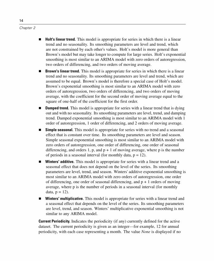
Holt's linear trend. This model is appropriate for series in which there is a lineartrend and no seasonality. Its smoothing parameters are level and trend, whichare not constrained by each other's values. Holt’s model is more general thanBrown’s model but may take longer to compute for large series. Holt’s exponentialsmoothing is most similar to an ARIMA model with zero orders of autoregression,two orders of differencing, and two orders of moving average.

Brown's linear trend. This model is appropriate for series in which there is a lineartrend and no seasonality. Its smoothing parameters are level and trend, which areassumed to be equal. Brown’s model is therefore a special case of Holt’s model.Brown’s exponential smoothing is most similar to an ARIMA model with zeroorders of autoregression, two orders of differencing, and two orders of movingaverage, with the coefficient for the second order of moving average equal to thesquare of one-half of the coefficient for the first order.

Damped trend. This model is appropriate for series with a linear trend that is dyingout and with no seasonality. Its smoothing parameters are level, trend, and dampingtrend. Damped exponential smoothing is most similar to an ARIMA model with 1order of autoregression, 1 order of differencing, and 2 orders of moving average.

Simple seasonal. This model is appropriate for series with no trend and a seasonaleffect that is constant over time. Its smoothing parameters are level and season.Simple seasonal exponential smoothing is most similar to an ARIMA model withzero orders of autoregression, one order of differencing, one order of seasonaldifferencing, and orders 1, p, and p + 1 of moving average, where p is the numberof periods in a seasonal interval (for monthly data, p = 12).

Winters' additive. This model is appropriate for series with a linear trend and aseasonal effect that does not depend on the level of the series. Its smoothingparameters are level, trend, and season. Winters' additive exponential smoothing ismost similar to an ARIMA model with zero orders of autoregression, one orderof differencing, one order of seasonal differencing, and p + 1 orders of movingaverage, where p is the number of periods in a seasonal interval (for monthlydata, p = 12).

Winters' multiplicative. This model is appropriate for series with a linear trend anda seasonal effect that depends on the level of the series. Its smoothing parametersare level, trend, and season. Winters’ multiplicative exponential smoothing is notsimilar to any ARIMA model.

Current Periodicity. Indicates the periodicity (if any) currently defined for the activedataset. The current periodicity is given as an integer—for example, 12 for annualperiodicity, with each case representing a month. The value None is displayed if no

15

Time Series Modeler

periodicity has been set. Seasonal models require a periodicity. You can set theperiodicity from the Define Dates dialog box.

Dependent Variable Transformation. You can specify a transformation performed oneach dependent variable before it is modeled.

None. No transformation is performed.

Square root. Square root transformation.

Natural log. Natural log transformation.

Custom ARIMA Models

The Time Series Modeler allows you to build custom nonseasonal or seasonal ARIMA(Autoregressive Integrated Moving Average) models—also known as Box-Jenkins(Box, Jenkins, and Reinsel, 1994) models—with or without a fixed set of predictorvariables. You can define transfer functions for any or all of the predictor variables,and specify automatic detection of outliers, or specify an explicit set of outliers.

All independent (predictor) variables specified on the Variables tab are explicitlyincluded in the model. This is in contrast to using the Expert Modeler whereindependent variables are only included if they have a statistically significantrelationship with the dependent variable.

16

Chapter 2

Model Specification for Custom ARIMA ModelsFigure 2-5ARIMA Criteria dialog box, Model tab

The Model tab allows you to specify the structure of a custom ARIMA model.

ARIMA Orders. Enter values for the various ARIMA components of your modelinto the corresponding cells of the Structure grid. All values must be non-negativeintegers. For autoregressive and moving average components, the value representsthe maximum order. All positive lower orders will be included in the model. Forexample, if you specify 2, the model includes orders 2 and 1. Cells in the Seasonalcolumn are only enabled if a periodicity has been defined for the active dataset (see“Current Periodicity” below).

17

Time Series Modeler

Autoregressive (p). The number of autoregressive orders in the model.Autoregressive orders specify which previous values from the series are used topredict current values. For example, an autoregressive order of 2 specifies that thevalue of the series two time periods in the past be used to predict the current value.

Difference (d). Specifies the order of differencing applied to the series beforeestimating models. Differencing is necessary when trends are present (series withtrends are typically nonstationary and ARIMA modeling assumes stationarity) andis used to remove their effect. The order of differencing corresponds to the degreeof series trend—first-order differencing accounts for linear trends, second-orderdifferencing accounts for quadratic trends, and so on.

Moving Average (q). The number of moving average orders in the model. Movingaverage orders specify how deviations from the series mean for previous valuesare used to predict current values. For example, moving-average orders of 1 and 2specify that deviations from the mean value of the series from each of the last twotime periods be considered when predicting current values of the series.

Seasonal Orders. Seasonal autoregressive, moving average, and differencingcomponents play the same roles as their nonseasonal counterparts. For seasonal orders,however, current series values are affected by previous series values separated by oneor more seasonal periods. For example, for monthly data (seasonal period of 12), aseasonal order of 1 means that the current series value is affected by the series value 12periods prior to the current one. A seasonal order of 1, for monthly data, is then thesame as specifying a nonseasonal order of 12.


Dependent Variable Transformation. You can specify a transformation performed oneach dependent variable before it is modeled.




Include constant in model. Inclusion of a constant is standard unless you are sure thatthe overall mean series value is 0. Excluding the constant is recommended whendifferencing is applied.

18

Chapter 2

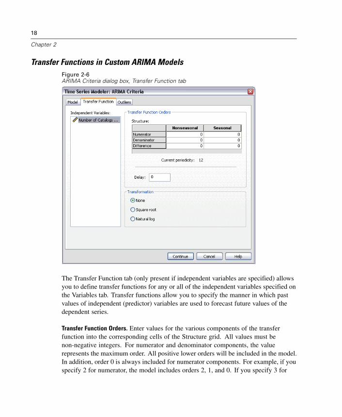
Transfer Functions in Custom ARIMA ModelsFigure 2-6ARIMA Criteria dialog box, Transfer Function tab

The Transfer Function tab (only present if independent variables are specified) allowsyou to define transfer functions for any or all of the independent variables specified onthe Variables tab. Transfer functions allow you to specify the manner in which pastvalues of independent (predictor) variables are used to forecast future values of thedependent series.

Transfer Function Orders. Enter values for the various components of the transferfunction into the corresponding cells of the Structure grid. All values must benon-negative integers. For numerator and denominator components, the valuerepresents the maximum order. All positive lower orders will be included in the model.In addition, order 0 is always included for numerator components. For example, if youspecify 2 for numerator, the model includes orders 2, 1, and 0. If you specify 3 for

19

Time Series Modeler

denominator, the model includes orders 3, 2, and 1. Cells in the Seasonal column areonly enabled if a periodicity has been defined for the active dataset (see “CurrentPeriodicity” below).

Numerator. The numerator order of the transfer function. Specifies which previousvalues from the selected independent (predictor) series are used to predict currentvalues of the dependent series. For example, a numerator order of 1 specifies thatthe value of an independent series one time period in the past—as well as thecurrent value of the independent series—is used to predict the current value ofeach dependent series.

Denominator. The denominator order of the transfer function. Specifies howdeviations from the series mean, for previous values of the selected independent(predictor) series, are used to predict current values of the dependent series. Forexample, a denominator order of 1 specifies that deviations from the mean value ofan independent series one time period in the past be considered when predictingthe current value of each dependent series.

Difference. Specifies the order of differencing applied to the selected independent(predictor) series before estimating models. Differencing is necessary when trendsare present and is used to remove their effect.

Seasonal Orders. Seasonal numerator, denominator, and differencing componentsplay the same roles as their nonseasonal counterparts. For seasonal orders, however,current series values are affected by previous series values separated by one or moreseasonal periods. For example, for monthly data (seasonal period of 12), a seasonalorder of 1 means that the current series value is affected by the series value 12 periodsprior to the current one. A seasonal order of 1, for monthly data, is then the sameas specifying a nonseasonal order of 12.


Delay. Setting a delay causes the independent variable’s influence to be delayed bythe number of intervals specified. For example, if the delay is set to 5, the value ofthe independent variable at time t doesn’t affect forecasts until five periods haveelapsed (t + 5).

20

Chapter 2

Transformation. Specification of a transfer function, for a set of independent variables,also includes an optional transformation to be performed on those variables.




Outliers in Custom ARIMA ModelsFigure 2-7ARIMA Criteria dialog box, Outliers tab

The Outliers tab provides the following choices for the handling of outliers (Pena,Tiao, and Tsay, 2001): detect them automatically, specify particular points as outliers,or do not detect or model them.

21

Time Series Modeler

Do not detect outliers or model them. By default, outliers are neither detected normodeled. Select this option to disable any detection or modeling of outliers.

Detect outliers automatically. Select this option to perform automatic detection ofoutliers, and select one or more of the following outlier types:

Additive

Level shift

Innovational

Transient

Seasonal additive

Local trend

Additive patch

For more information, see “Outlier Types” in Appendix B on p. 127.

Model specific time points as outliers. Select this option to specify particular time pointsas outliers. Use a separate row of the Outlier Definition grid for each outlier. Entervalues for all of the cells in a given row.

Type. The outlier type. The supported types are: additive (default), level shift,innovational, transient, seasonal additive, and local trend.

Note 1: If no date specification has been defined for the active dataset, the OutlierDefinition grid shows the single column Observation. To specify an outlier, enter therow number (as displayed in the Data Editor) of the relevant case.

Note 2: The Cycle column (if present) in the Outlier Definition grid refers to the valueof the CYCLE_ variable in the active dataset.

Output

Available output includes results for individual models as well as results calculatedacross all models. Results for individual models can be limited to a set of best- orpoorest-fitting models based on user-specified criteria.

22

Chapter 2

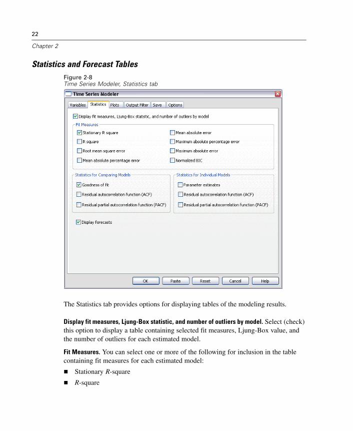
Statistics and Forecast TablesFigure 2-8Time Series Modeler, Statistics tab

The Statistics tab provides options for displaying tables of the modeling results.

Display fit measures, Ljung-Box statistic, and number of outliers by model. Select (check)this option to display a table containing selected fit measures, Ljung-Box value, andthe number of outliers for each estimated model.

Fit Measures. You can select one or more of the following for inclusion in the tablecontaining fit measures for each estimated model:

Stationary R-square

R-square

23

Time Series Modeler

Root mean square error

Mean absolute percentage error

Mean absolute error

Maximum absolute percentage error

Maximum absolute error

Normalized BIC

For more information, see “Goodness-of-Fit Measures” in Appendix A on p. 125.

Statistics for Comparing Models. This group of options controls display of tablescontaining statistics calculated across all estimated models. Each option generates aseparate table. You can select one or more of the following options:

Goodness of fit. Table of summary statistics and percentiles for stationary R-square,R-square, root mean square error, mean absolute percentage error, mean absoluteerror, maximum absolute percentage error, maximum absolute error, andnormalized Bayesian Information Criterion.

Residual autocorrelation function (ACF). Table of summary statistics and percentilesfor autocorrelations of the residuals across all estimated models.

Residual partial autocorrelation function (PACF). Table of summary statistics andpercentiles for partial autocorrelations of the residuals across all estimated models.

Statistics for Individual Models. This group of options controls display of tablescontaining detailed information for each estimated model. Each option generates aseparate table. You can select one or more of the following options:

Parameter estimates. Displays a table of parameter estimates for each estimatedmodel. Separate tables are displayed for exponential smoothing and ARIMAmodels. If outliers exist, parameter estimates for them are also displayed in aseparate table.

Residual autocorrelation function (ACF). Displays a table of residual autocorrelationsby lag for each estimated model. The table includes the confidence intervals forthe autocorrelations.

Residual partial autocorrelation function (PACF). Displays a table of residualpartial autocorrelations by lag for each estimated model. The table includes theconfidence intervals for the partial autocorrelations.

Display forecasts. Displays a table of model forecasts and confidence intervals for eachestimated model. The forecast period is set from the Options tab.

24

Chapter 2

PlotsFigure 2-9Time Series Modeler, Plots tab

The Plots tab provides options for displaying plots of the modeling results.

Plots for Comparing Models

This group of options controls display of plots containing statistics calculated acrossall estimated models. Each option generates a separate plot. You can select one ormore of the following options:

Stationary R-square

R-square

25

Time Series Modeler



Mean absolute error



Normalized BIC

Residual autocorrelation function (ACF)

Residual partial autocorrelation function (PACF)


Plots for Individual Models

Series. Select (check) this option to obtain plots of the predicted values for eachestimated model. You can select one or more of the following for inclusion in the plot:

Observed values. The observed values of the dependent series.

Forecasts. The model predicted values for the forecast period.

Fit values. The model predicted values for the estimation period.

Confidence intervals for forecasts. The confidence intervals for the forecast period.

Confidence intervals for fit values. The confidence intervals for the estimationperiod.

Residual autocorrelation function (ACF). Displays a plot of residual autocorrelations foreach estimated model.

Residual partial autocorrelation function (PACF). Displays a plot of residual partialautocorrelations for each estimated model.

26

Chapter 2

Limiting Output to the Best- or Poorest-Fitting Models

Figure 2-10Time Series Modeler, Output Filter tab

The Output Filter tab provides options for restricting both tabular and chart output toa subset of the estimated models. You can choose to limit output to the best-fittingand/or the poorest-fitting models according to fit criteria you provide. By default, allestimated models are included in the output.

Best-fitting models. Select (check) this option to include the best-fitting models in theoutput. Select a goodness-of-fit measure and specify the number of models to include.Selecting this option does not preclude also selecting the poorest-fitting models. In thatcase, the output will consist of the poorest-fitting models as well as the best-fitting ones.

27

Time Series Modeler

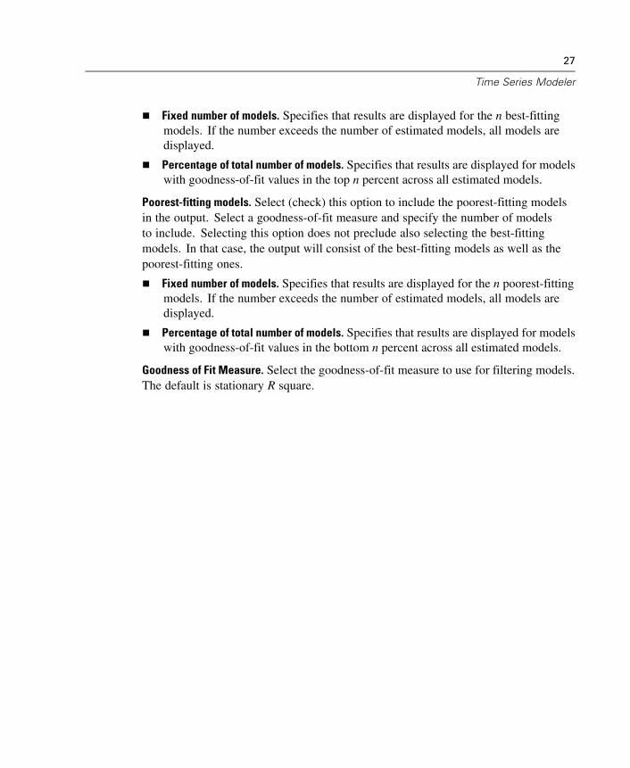
Fixed number of models. Specifies that results are displayed for the n best-fittingmodels. If the number exceeds the number of estimated models, all models aredisplayed.

Percentage of total number of models. Specifies that results are displayed for modelswith goodness-of-fit values in the top n percent across all estimated models.

Poorest-fitting models. Select (check) this option to include the poorest-fitting modelsin the output. Select a goodness-of-fit measure and specify the number of modelsto include. Selecting this option does not preclude also selecting the best-fittingmodels. In that case, the output will consist of the best-fitting models as well as thepoorest-fitting ones.

Fixed number of models. Specifies that results are displayed for the n poorest-fittingmodels. If the number exceeds the number of estimated models, all models aredisplayed.

Percentage of total number of models. Specifies that results are displayed for modelswith goodness-of-fit values in the bottom n percent across all estimated models.

Goodness of Fit Measure. Select the goodness-of-fit measure to use for filtering models.The default is stationary R square.

28

Chapter 2

Saving Model Predictions and Model SpecificationsFigure 2-11Time Series Modeler, Save tab

The Save tab allows you to save model predictions as new variables in the activedataset and save model specifications to an external file in XML format.

Save Variables. You can save model predictions, confidence intervals, and residualsas new variables in the active dataset. Each dependent series gives rise to its ownset of new variables, and each new variable contains values for both the estimationand forecast periods. New cases are added if the forecast period extends beyond thelength of the dependent variable series. Choose to save new variables by selecting theassociated Save check box for each. By default, no new variables are saved.

Predicted Values. The model predicted values.

29

Time Series Modeler

Lower Confidence Limits. Lower confidence limits for the predicted values.

Upper Confidence Limits. Upper confidence limits for the predicted values.

Noise Residuals. The model residuals. When transformations of the dependentvariable are performed (for example, natural log), these are the residuals for thetransformed series.

Variable Name Prefix. Specify prefixes to be used for new variable names, orleave the default prefixes. Variable names consist of the prefix, the name ofthe associated dependent variable, and a model identifier. The variable name isextended if necessary to avoid variable naming conflicts. The prefix must conformto the rules for valid SPSS variable names.

Export Model File. Model specifications for all estimated models are exported to thespecified file in XML format. Saved models can be used to obtain updated forecasts,based on more current data, using the “Apply Time Series Models” procedure.

30

Chapter 2

OptionsFigure 2-12Time Series Modeler, Options tab

The Options tab allows you to set the forecast period, specify the handling of missingvalues, set the confidence interval width, specify a custom prefix for model identifiers,and set the number of lags shown for autocorrelations.

Forecast Period. The forecast period always begins with the first case after the end ofthe estimation period (the set of cases used to determine the model) and goes througheither the last case in the active dataset or a user-specified date. By default, the end ofthe estimation period is the last case in the active dataset, but it can be changed fromthe Select Cases dialog box by selecting Based on time or case range.

31

Time Series Modeler

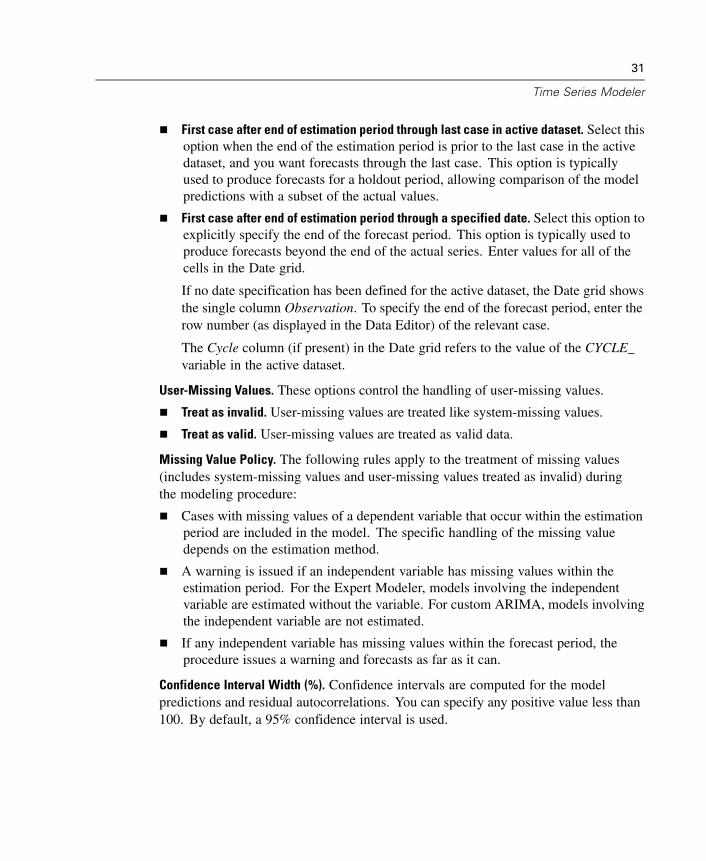
First case after end of estimation period through last case in active dataset. Select thisoption when the end of the estimation period is prior to the last case in the activedataset, and you want forecasts through the last case. This option is typicallyused to produce forecasts for a holdout period, allowing comparison of the modelpredictions with a subset of the actual values.

First case after end of estimation period through a specified date. Select this option toexplicitly specify the end of the forecast period. This option is typically used toproduce forecasts beyond the end of the actual series. Enter values for all of thecells in the Date grid.

If no date specification has been defined for the active dataset, the Date grid showsthe single column Observation. To specify the end of the forecast period, enter therow number (as displayed in the Data Editor) of the relevant case.

The Cycle column (if present) in the Date grid refers to the value of the CYCLE_variable in the active dataset.

User-Missing Values. These options control the handling of user-missing values.

Treat as invalid. User-missing values are treated like system-missing values.

Treat as valid. User-missing values are treated as valid data.

Missing Value Policy. The following rules apply to the treatment of missing values(includes system-missing values and user-missing values treated as invalid) duringthe modeling procedure:

Cases with missing values of a dependent variable that occur within the estimationperiod are included in the model. The specific handling of the missing valuedepends on the estimation method.

A warning is issued if an independent variable has missing values within theestimation period. For the Expert Modeler, models involving the independentvariable are estimated without the variable. For custom ARIMA, models involvingthe independent variable are not estimated.

If any independent variable has missing values within the forecast period, theprocedure issues a warning and forecasts as far as it can.

Confidence Interval Width (%). Confidence intervals are computed for the modelpredictions and residual autocorrelations. You can specify any positive value less than100. By default, a 95% confidence interval is used.

32

Chapter 2

Prefix for Model Identifiers in Output. Each dependent variable specified on the Variablestab gives rise to a separate estimated model. Models are distinguished with uniquenames consisting of a customizable prefix along with an integer suffix. You can entera prefix or leave the default of Model.

Maximum Number of Lags Shown in ACF and PACF Output. You can set themaximum number of lags shown in tables and plots of autocorrelations and partialautocorrelations.

TSMODEL Command Additional Features

You can customize your time series modeling if you paste your selections into a syntaxwindow and edit the resulting TSMODEL command syntax. SPSS command languageallows you to:

Specify the seasonal period of the data (with the SEASONLENGTH keyword onthe AUXILIARY subcommand). This overrides the current periodicity (if any)for the active dataset.

Specify nonconsecutive lags for custom ARIMA and transfer function components(with the ARIMA and TRANSFERFUNCTION subcommands). For example, you canspecify a custom ARIMA model with autoregressive lags of orders 1, 3, and 6; or atransfer function with numerator lags of orders 2, 5, and 8.

Provide more than one set of modeling specifications (for example, modelingmethod, ARIMA orders, independent variables, and so on) for a single run of theTime Series Modeler procedure (with the MODEL subcommand).

See the SPSS Command Syntax Reference for complete syntax information.

Chapter

3Apply Time Series Models

The Apply Time Series Models procedure loads existing time series models from anexternal file and applies them to the active dataset. You can use this procedure to obtainforecasts for series for which new or revised data are available, without rebuilding yourmodels. Models are generated using the “Time Series Modeler” procedure.

Example. You are an inventory manager with a major retailer, and responsible for eachof 5,000 products. You’ve used the Expert Modeler to create models that forecast salesfor each product three months into the future. Your data warehouse is refreshed eachmonth with actual sales data which you’d like to use to produce monthly updatedforecasts. The Apply Time Series Models procedure allows you to accomplish thisusing the original models, and simply reestimating model parameters to account forthe new data.

Statistics. Goodness-of-fit measures: stationary R-square, R-square (R2), root meansquare error (RMSE), mean absolute error (MAE), mean absolute percentageerror (MAPE), maximum absolute error (MaxAE), maximum absolute percentageerror (MaxAPE), normalized Bayesian information criterion (BIC). Residuals:autocorrelation function, partial autocorrelation function, Ljung-Box Q.

Plots. Summary plots across all models: histograms of stationary R-square, R-square(R2), root mean square error (RMSE), mean absolute error (MAE), mean absolutepercentage error (MAPE), maximum absolute error (MaxAE), maximum absolutepercentage error (MaxAPE), normalized Bayesian information criterion (BIC); boxplots of residual autocorrelations and partial autocorrelations. Results for individualmodels: forecast values, fit values, observed values, upper and lower confidence limits,residual autocorrelations and partial autocorrelations.

Apply Time Series Models Data Considerations

Data. Variables (dependent and independent) to which models will be applied shouldbe numeric.

33

34

Chapter 3

Assumptions. Models are applied to variables in the active dataset with the same namesas the variables specified in the model. All such variables are treated as time series,meaning that each case represents a time point, with successive cases separated by aconstant time interval.

Forecasts. For producing forecasts using models with independent (predictor)variables, the active dataset should contain values of these variables for all casesin the forecast period. If model parameters are reestimated, then independentvariables should not contain any missing values in the estimation period.

Defining Dates

The Apply Time Series Models procedure requires that the periodicity, if any, of theactive dataset matches the periodicity of the models to be applied. If you’re simplyforecasting using the same dataset (perhaps with new or revised data) as that used tothe build the model, then this condition will be satisfied. If no periodicity exists forthe active dataset, you will be given the opportunity to navigate to the Define Datesdialog box to create one. If, however, the models were created without specifying aperiodicity, then the active dataset should also be without one.

To Apply Models

From the menus choose:Analyze

Time SeriesApply Models...

35

Apply Time Series Models

Figure 3-1Apply Time Series Models, Models tab

E Enter the file specification for a model file or click Browse and select a model file(model files are created with the “Time Series Modeler” procedure).


Reestimate model parameters using the data in the active dataset. Forecasts arecreated using the reestimated parameters.

Save predictions, confidence intervals, and noise residuals.

Save reestimated models in XML format.

36

Chapter 3

Model Parameters and Goodness of Fit Measures

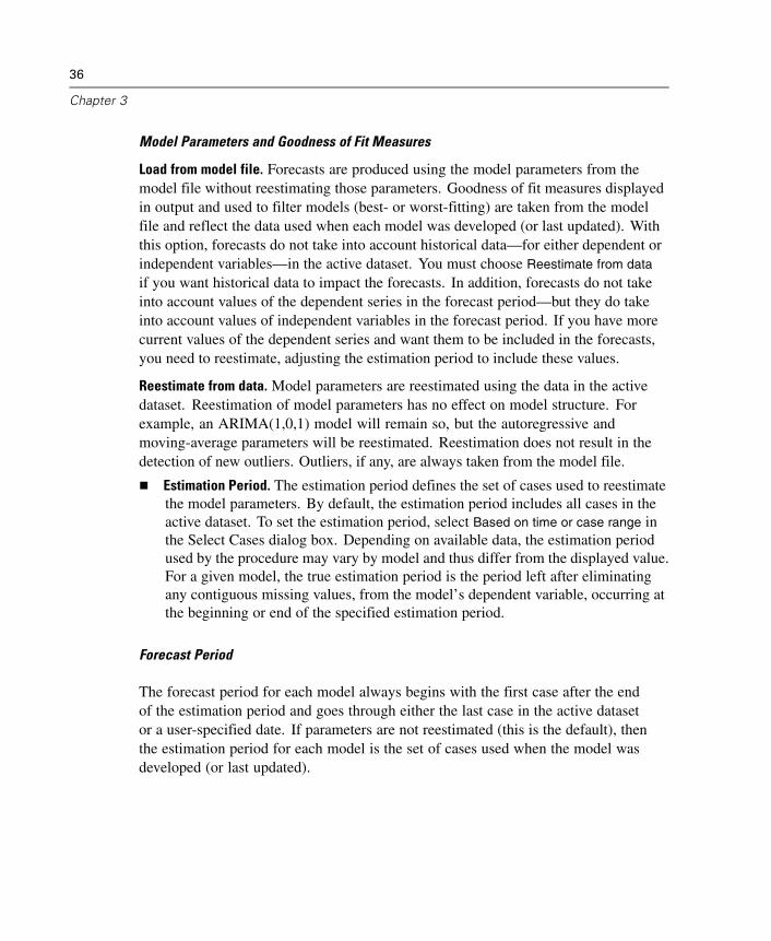
Load from model file. Forecasts are produced using the model parameters from themodel file without reestimating those parameters. Goodness of fit measures displayedin output and used to filter models (best- or worst-fitting) are taken from the modelfile and reflect the data used when each model was developed (or last updated). Withthis option, forecasts do not take into account historical data—for either dependent orindependent variables—in the active dataset. You must choose Reestimate from data

if you want historical data to impact the forecasts. In addition, forecasts do not takeinto account values of the dependent series in the forecast period—but they do takeinto account values of independent variables in the forecast period. If you have morecurrent values of the dependent series and want them to be included in the forecasts,you need to reestimate, adjusting the estimation period to include these values.

Reestimate from data. Model parameters are reestimated using the data in the activedataset. Reestimation of model parameters has no effect on model structure. Forexample, an ARIMA(1,0,1) model will remain so, but the autoregressive andmoving-average parameters will be reestimated. Reestimation does not result in thedetection of new outliers. Outliers, if any, are always taken from the model file.

Estimation Period. The estimation period defines the set of cases used to reestimatethe model parameters. By default, the estimation period includes all cases in theactive dataset. To set the estimation period, select Based on time or case range inthe Select Cases dialog box. Depending on available data, the estimation periodused by the procedure may vary by model and thus differ from the displayed value.For a given model, the true estimation period is the period left after eliminatingany contiguous missing values, from the model’s dependent variable, occurring atthe beginning or end of the specified estimation period.

Forecast Period

The forecast period for each model always begins with the first case after the endof the estimation period and goes through either the last case in the active datasetor a user-specified date. If parameters are not reestimated (this is the default), thenthe estimation period for each model is the set of cases used when the model wasdeveloped (or last updated).

37


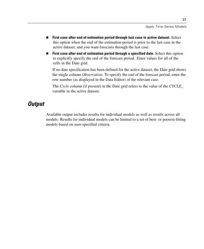
First case after end of estimation period through last case in active dataset. Selectthis option when the end of the estimation period is prior to the last case in theactive dataset, and you want forecasts through the last case.

First case after end of estimation period through a specified date. Select this optionto explicitly specify the end of the forecast period. Enter values for all of thecells in the Date grid.

If no date specification has been defined for the active dataset, the Date grid showsthe single column Observation. To specify the end of the forecast period, enter therow number (as displayed in the Data Editor) of the relevant case.

The Cycle column (if present) in the Date grid refers to the value of the CYCLE_variable in the active dataset.

Output

Available output includes results for individual models as well as results across allmodels. Results for individual models can be limited to a set of best- or poorest-fittingmodels based on user-specified criteria.

38

Chapter 3

Statistics and Forecast TablesFigure 3-2Apply Time Series Models, Statistics tab

The Statistics tab provides options for displaying tables of model fit statistics, modelparameters, autocorrelation functions, and forecasts. Unless model parameters arereestimated (Reestimate from data on the Models tab), displayed values of fit measures,Ljung-Box values, and model parameters are those from the model file and reflect thedata used when each model was developed (or last updated). Outlier information isalways taken from the model file.

39


Display fit measures, Ljung-Box statistic, and number of outliers by model. Select (check)this option to display a table containing selected fit measures, Ljung-Box value, andthe number of outliers for each model.

Fit Measures. You can select one or more of the following for inclusion in the tablecontaining fit measures for each model:

Stationary R-square

R-square



Mean absolute error



Normalized BIC


Statistics for Comparing Models. This group of options controls the display of tablescontaining statistics across all models. Each option generates a separate table. You canselect one or more of the following options:

Goodness of fit. Table of summary statistics and percentiles for stationary R-square,R-square, root mean square error, mean absolute percentage error, mean absoluteerror, maximum absolute percentage error, maximum absolute error, andnormalized Bayesian Information Criterion.

Residual autocorrelation function (ACF). Table of summary statistics and percentilesfor autocorrelations of the residuals across all estimated models. This table isonly available if model parameters are reestimated (Reestimate from data on theModels tab).

Residual partial autocorrelation function (PACF). Table of summary statistics andpercentiles for partial autocorrelations of the residuals across all estimated models.This table is only available if model parameters are reestimated (Reestimate fromdata on the Models tab).

40

Chapter 3

Statistics for Individual Models. This group of options controls display of tablescontaining detailed information for each model. Each option generates a separatetable. You can select one or more of the following options:

Parameter estimates. Displays a table of parameter estimates for each model.Separate tables are displayed for exponential smoothing and ARIMA models. Ifoutliers exist, parameter estimates for them are also displayed in a separate table.

Residual autocorrelation function (ACF). Displays a table of residual autocorrelationsby lag for each estimated model. The table includes the confidence intervalsfor the autocorrelations. This table is only available if model parameters arereestimated (Reestimate from data on the Models tab).

Residual partial autocorrelation function (PACF). Displays a table of residualpartial autocorrelations by lag for each estimated model. The table includes theconfidence intervals for the partial autocorrelations. This table is only available ifmodel parameters are reestimated (Reestimate from data on the Models tab).

Display forecasts. Displays a table of model forecasts and confidence intervals foreach model.

41


PlotsFigure 3-3Apply Time Series Models, Plots tab

The Plots tab provides options for displaying plots of model fit statistics,autocorrelation functions, and series values (including forecasts).

Plots for Comparing Models

This group of options controls the display of plots containing statistics across allmodels. Unless model parameters are reestimated (Reestimate from data on the Modelstab), displayed values are those from the model file and reflect the data used when each

42

Chapter 3

model was developed (or last updated). In addition, autocorrelation plots are onlyavailable if model parameters are reestimated. Each option generates a separate plot.You can select one or more of the following options:

Stationary R-square

R-square



Mean absolute error



Normalized BIC

Residual autocorrelation function (ACF)

Residual partial autocorrelation function (PACF)


Plots for Individual Models

Series. Select (check) this option to obtain plots of the predicted values for each model.Observed values, fit values, confidence intervals for fit values, and autocorrelationsare only available if model parameters are reestimated (Reestimate from data on theModels tab). You can select one or more of the following for inclusion in the plot:

Observed values. The observed values of the dependent series.

Forecasts. The model predicted values for the forecast period.

Fit values. The model predicted values for the estimation period.

Confidence intervals for forecasts. The confidence intervals for the forecast period.

Confidence intervals for fit values. The confidence intervals for the estimationperiod.

Residual autocorrelation function (ACF). Displays a plot of residual autocorrelations foreach estimated model.

Residual partial autocorrelation function (PACF). Displays a plot of residual partialautocorrelations for each estimated model.

43


Limiting Output to the Best- or Poorest-Fitting ModelsFigure 3-4Apply Time Series Models, Output Filter tab

The Output Filter tab provides options for restricting both tabular and chart outputto a subset of models. You can choose to limit output to the best-fitting and/or thepoorest-fitting models according to fit criteria you provide. By default, all models areincluded in the output. Unless model parameters are reestimated (Reestimate from data

on the Models tab), values of fit measures used for filtering models are those from themodel file and reflect the data used when each model was developed (or last updated).

44

Chapter 3

Best-fitting models. Select (check) this option to include the best-fitting models in theoutput. Select a goodness-of-fit measure and specify the number of models to include.Selecting this option does not preclude also selecting the poorest-fitting models. In thatcase, the output will consist of the poorest-fitting models as well as the best-fitting ones.

Fixed number of models. Specifies that results are displayed for the n best-fittingmodels. If the number exceeds the total number of models, all models aredisplayed.

Percentage of total number of models. Specifies that results are displayed for modelswith goodness-of-fit values in the top n percent across all models.

Poorest-fitting models. Select (check) this option to include the poorest-fitting modelsin the output. Select a goodness-of-fit measure and specify the number of modelsto include. Selecting this option does not preclude also selecting the best-fittingmodels. In that case, the output will consist of the best-fitting models as well as thepoorest-fitting ones.

Fixed number of models. Specifies that results are displayed for the n poorest-fittingmodels. If the number exceeds the total number of models, all models aredisplayed.

Percentage of total number of models. Specifies that results are displayed for modelswith goodness-of-fit values in the bottom n percent across all models.

Goodness of Fit Measure. Select the goodness-of-fit measure to use for filtering models.The default is stationary R-square.

45


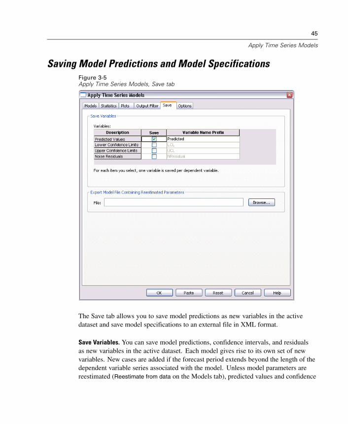
Saving Model Predictions and Model SpecificationsFigure 3-5Apply Time Series Models, Save tab

The Save tab allows you to save model predictions as new variables in the activedataset and save model specifications to an external file in XML format.

Save Variables. You can save model predictions, confidence intervals, and residualsas new variables in the active dataset. Each model gives rise to its own set of newvariables. New cases are added if the forecast period extends beyond the length of thedependent variable series associated with the model. Unless model parameters arereestimated (Reestimate from data on the Models tab), predicted values and confidence

46

Chapter 3

limits are only created for the forecast period. Choose to save new variables byselecting the associated Save check box for each. By default, no new variables aresaved.

Predicted Values. The model predicted values.

Lower Confidence Limits. Lower confidence limits for the predicted values.

Upper Confidence Limits. Upper confidence limits for the predicted values.

Noise Residuals. The model residuals. When transformations of the dependentvariable are performed (for example, natural log), these are the residuals forthe transformed series. This choice is only available if model parameters arereestimated (Reestimate from data on the Models tab).

Variable Name Prefix. Specify prefixes to be used for new variable names orleave the default prefixes. Variable names consist of the prefix, the name ofthe associated dependent variable, and a model identifier. The variable name isextended if necessary to avoid variable naming conflicts. The prefix must conformto the rules for valid SPSS variable names.

Export Model File Containing Reestimated Parameters. Model specifications, containingreestimated parameters and fit statistics, are exported to the specified file in XMLformat. This option is only available if model parameters are reestimated (Reestimate

from data on the Models tab).

47


OptionsFigure 3-6Apply Time Series Models, Options tab

The Options tab allows you to specify the handling of missing values, set theconfidence interval width, and set the number of lags shown for autocorrelations.

User-Missing Values. These options control the handling of user-missing values.

Treat as invalid. User-missing values are treated like system-missing values.

Treat as valid. User-missing values are treated as valid data.

48

Chapter 3

Missing Value Policy. The following rules apply to the treatment of missing values(includes system-missing values and user-missing values treated as invalid):

Cases with missing values of a dependent variable that occur within the estimationperiod are included in the model. The specific handling of the missing valuedepends on the estimation method.

For ARIMA models, a warning is issued if a predictor has any missing valueswithin the estimation period. Any models involving the predictor are notreestimated.

If any independent variable has missing values within the forecast period, theprocedure issues a warning and forecasts as far as it can.

Confidence Interval Width (%). Confidence intervals are computed for the modelpredictions and residual autocorrelations. You can specify any positive value less than100. By default, a 95% confidence interval is used.

Maximum Number of Lags Shown in ACF and PACF Output. You can set themaximum number of lags shown in tables and plots of autocorrelations and partialautocorrelations. This option is only available if model parameters are reestimated(Reestimate from data on the Models tab).

TSAPPLY Command Additional Features

Additional features are available if you paste your selections into a syntax window andedit the resulting TSAPPLY command syntax. SPSS command language allows you to:

Specify that only a subset of the models in a model file are to be applied to theactive dataset (with the DROP and KEEP keywords on the MODEL subcommand).

Apply models from two or more model files to your data (with the MODELsubcommand). For example, one model file might contain models for series thatrepresent unit sales, and another might contain models for series that representrevenue.


Chapter

4Seasonal Decomposition

The Seasonal Decomposition procedure decomposes a series into a seasonalcomponent, a combined trend and cycle component, and an “error” component. Theprocedure is an implementation of the Census Method I, otherwise known as theratio-to-moving-average method.

Example. A scientist is interested in analyzing monthly measurements of the ozonelevel at a particular weather station. The goal is to determine if there is any trend inthe data. In order to uncover any real trend, the scientist first needs to account for thevariation in readings due to seasonal effects. The Seasonal Decomposition procedurecan be used to remove any systematic seasonal variations. The trend analysis is thenperformed on a seasonally adjusted series.

Statistics. The set of seasonal factors.

Data. The variables should be numeric.

Assumptions. The variables should not contain any embedded missing data. At leastone periodic date component must be defined.

Estimating Seasonal Factors

E From the menus choose:Analyze

Time SeriesSeasonal Decomposition...

49

50

Chapter 4

Figure 4-1Seasonal Decomposition dialog box

E Select one or more variables from the available list and move them into the Variable(s)list. Note that the list includes only numeric variables.

Model. The Seasonal Decomposition procedure offers two different approaches formodeling the seasonal factors: multiplicative or additive.

Multiplicative. The seasonal component is a factor by which the seasonally adjustedseries is multiplied to yield the original series. In effect, Trends estimates seasonalcomponents that are proportional to the overall level of the series. Observationswithout seasonal variation have a seasonal component of 1.

Additive. The seasonal adjustments are added to the seasonally adjusted seriesto obtain the observed values. This adjustment attempts to remove the seasonaleffect from a series in order to look at other characteristics of interest that maybe "masked" by the seasonal component. In effect, Trends estimates seasonalcomponents that do not depend on the overall level of the series. Observationswithout seasonal variation have a seasonal component of 0.

Moving Average Weight. The Moving Average Weight options allow you to specify howto treat the series when computing moving averages. These options are availableonly if the periodicity of the series is even. If the periodicity is odd, all points areweighted equally.

51

Seasonal Decomposition

All points equal. Moving averages are calculated with a span equal to the periodicityand with all points weighted equally. This method is always used if the periodicityis odd.

Endpoints weighted by .5. Moving averages for series with even periodicity arecalculated with a span equal to the periodicity plus 1 and with the endpoints of thespan weighted by 0.5.


Click Save to specify how new variables should be saved.

Seasonal Decomposition SaveFigure 4-2Season Save dialog box

Create Variables. Allows you to choose how to treat new variables.

Add to file. The new series created by Seasonal Decomposition are saved as regularvariables in your active dataset. Variable names are formed from a three-letterprefix, an underscore, and a number.

Replace existing. The new series created by Seasonal Decomposition are savedas temporary variables in your active dataset. At the same time, any existingtemporary variables created by the Trends procedures are dropped. Variable namesare formed from a three-letter prefix, a pound sign (#), and a number.

Do not create. The new series are not added to the active dataset.

New Variable Names

The Seasonal Decomposition procedure creates four new variables (series), with thefollowing three-letter prefixes, for each series specified:

SAF. Seasonal adjustment factors. These values indicate the effect of each periodon the level of the series.

52

Chapter 4

SAS. Seasonally adjusted series. These are the values obtained after removing theseasonal variation of a series.

STC. Smoothed trend-cycle components. These values show the trend and cyclicalbehavior present in the series.

ERR. Residual or “error” values. The values that remain after the seasonal, trend,and cycle components have been removed from the series.

SEASON Command Additional Features

The SPSS command language also allows you to:

Specify any periodicity within the SEASON command rather than select one of thealternatives offered by the Define Dates procedure.


Chapter

5Spectral Plots

The Spectral Plots procedure is used to identify periodic behavior in time series.Instead of analyzing the variation from one time point to the next, it analyzes thevariation of the series as a whole into periodic components of different frequencies.Smooth series have stronger periodic components at low frequencies; random variation(“white noise”) spreads the component strength over all frequencies.

Series that include missing data cannot be analyzed with this procedure.

Example. The rate at which new houses are constructed is an important barometer ofthe state of the economy. Data for housing starts typically exhibit a strong seasonalcomponent. But are there longer cycles present in the data that analysts need to beaware of when evaluating current figures?

Statistics. Sine and cosine transforms, periodogram value, and spectral density estimatefor each frequency or period component. When bivariate analysis is selected: real andimaginary parts of cross-periodogram, cospectral density, quadrature spectrum, gain,squared coherency, and phase spectrum for each frequency or period component.

Plots. For univariate and bivariate analyses: periodogram and spectral density.For bivariate analyses: squared coherency, quadrature spectrum, cross amplitude,cospectral density, phase spectrum, and gain.

Data. The variables should be numeric.

Assumptions. The variables should not contain any embedded missing data. The timeseries to be analyzed should be stationary and any non-zero mean should be subtractedout from the series.

Stationary. A condition that must be met by the time series to which you fit anARIMA model. Pure MA series will be stationary; however, AR and ARMAseries might not be. A stationary series has a constant mean and a constantvariance over time.

53

54

Chapter 5

Obtaining a Spectral Analysis

E From the menus choose:Graphs

Time SeriesSpectral...

Figure 5-1Spectral Plots dialog box

E Select one or more variables from the available list and move them to the Variable(s)list. Note that the list includes only numeric variables.

E Select one of the Spectral Window options to choose how to smooth the periodogramin order to obtain a spectral density estimate. Available smoothing options areTukey-Hamming, Tukey, Parzen, Bartlett, Daniell (Unit), and None.

Tukey-Hamming. The weights are Wk = .54Dp(2 pi fk) + .23Dp (2 pi fk + pi/p) +.23Dp (2 pi fk - pi/p), for k = 0, ..., p, where p is the integer part of half the spanand Dp is the Dirichlet kernel of order p.

Tukey. The weights are Wk = 0.5Dp(2 pi fk) + 0.25Dp (2 pi fk + pi/p) + 0.25Dp(2pi fk - pi/p), for k = 0, ..., p, where p is the integer part of half the span and Dp isthe Dirichlet kernel of order p.

Parzen. The weights are Wk = 1/p(2 + cos(2 pi fk)) (F[p/2] (2 pi fk))**2, for k=0, ... p, where p is the integer part of half the span and F[p/2] is the Fejer kernelof order p/2.

55

Spectral Plots

Bartlett. The shape of a spectral window for which the weights of the upper halfof the window are computed as Wk = Fp (2*pi*fk), for k = 0, ... p, where p isthe integer part of half the span and Fp is the Fejer kernel of order p. The lowerhalf is symmetric with the upper half.

Daniell (Unit). The shape of a spectral window for which the weights are all equalto 1.

None. No smoothing. If this option is chosen, the spectral density estimate isthe same as the periodogram.

Bivariate analysis – first variable with each. If you have selected two or more variables,you can select this option to request bivariate spectral analyses.

The first variable in the Variable(s) list is treated as the independent variable, andall remaining variables are treated as dependent variables.

Each series after the first is analyzed with the first series independently of otherseries named. Univariate analyses of each series are also performed.

Span. The range of consecutive values across which the smoothing is carried out.Generally, an odd integer is used. Larger spans smooth the spectral density plot morethan smaller spans.

Center variables. Adjusts the series to have a mean of 0 before calculating the spectrumand to remove the large term that may be associated with the series mean.

Plot. Periodogram and spectral density are available for both univariate and bivariateanalyses. All other choices are available only for bivariate analyses.

Periodogram. Unsmoothed plot of spectral amplitude (plotted on a logarithmicscale) against either frequency or period. Low-frequency variation characterizesa smooth series. Variation spread evenly across all frequencies indicates "whitenoise."

Spectral density. A periodogram that has been smoothed to remove irregularvariation.

Cospectral density. The real part of the cross-periodogram, which is a measure ofthe correlation of the in-phase frequency components of two time series.

Quadrature spectrum. The imaginary part of the cross-periodogram, which is ameasure of the correlation of the out-of-phase frequency components of two timeseries. The components are out of phase by pi/2 radians.

Cross amplitude. The square root of the sum of the squared cospectral densityand the squared quadrature spectrum.

56

Chapter 5

Gain. The quotient of dividing the cross amplitude by the spectral density for oneof the series. Each of the two series has its own gain value.

Squared coherency. The product of the gains of the two series.

Phase spectrum. A measure of the extent to which each frequency component ofone series leads or lags the other.

By frequency. All plots are produced by frequency, ranging from frequency 0 (theconstant or mean term) to frequency 0.5 (the term for a cycle of two observations).

By period. All plots are produced by period, ranging from 2 (the term for a cycle of twoobservations) to a period equal to the number of observations (the constant or meanterm). Period is displayed on a logarithmic scale.

SPECTRA Command Additional Features

The SPSS command language also allows you to:

Save computed spectral analysis variables to the active dataset for later use.

Specify custom weights for the spectral window.

Produce plots by both frequency and period.

Print a complete listing of each value shown in the plot.


Part II:Examples

Chapter

6Bulk Forecasting with the ExpertModeler

An analyst for a national broadband provider is required to produce forecasts ofuser subscriptions in order to predict utilization of bandwidth. Forecasts are neededfor each of the 85 local markets that make up the national subscriber base. Monthlyhistorical data is collected in broadband_1.sav, found in the \tutorial\sample_files\folder where SPSS was installed.

In this example, you will use the Expert Modeler to produce forecasts for the nextthree months for each of the 85 local markets, saving the generated models to anexternal XML file. Once you are finished, you might want to work through the nextexample, “Bulk Reforecasting by Applying Saved Models” in Chapter 7 on p. 73,which applies the saved models to an updated dataset in order to extend the forecastsby another three months without having to rebuild the models.

Examining Your Data

It is always a good idea to have a feel for the nature of your data before building amodel. Does the data exhibit seasonal variations? Although the Expert Modelerwill automatically find the best seasonal or non-seasonal model for each series, youcan often obtain faster results by limiting the search to non-seasonal models whenseasonality is not present in your data. Without examining the data for each of the 85local markets, we can get a rough picture by plotting the total number of subscribersover all markets.


Sequence...

59

60

Chapter 6

Figure 6-1Sequence Charts dialog box

E Select Total Number of Subscribers and move it into the Variables list.

E Select Date and move it into the Time Axis Labels box.

E Click OK.

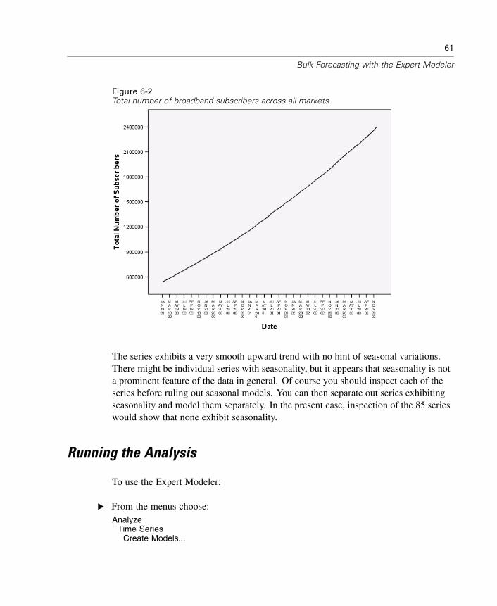
61

Bulk Forecasting with the Expert Modeler

Figure 6-2Total number of broadband subscribers across all markets

The series exhibits a very smooth upward trend with no hint of seasonal variations.There might be individual series with seasonality, but it appears that seasonality is nota prominent feature of the data in general. Of course you should inspect each of theseries before ruling out seasonal models. You can then separate out series exhibitingseasonality and model them separately. In the present case, inspection of the 85 serieswould show that none exhibit seasonality.

Running the Analysis

To use the Expert Modeler:



62

Chapter 6

Figure 6-3Time Series Modeler dialog box

E Select Subscribers for Market 1 through Subscribers for Market 85 for dependentvariables.

E Verify that Expert Modeler is selected in the Method drop-down list. The ExpertModeler will automatically find the best-fitting model for each of the dependentvariable series.

The set of cases used to estimate the model is referred to as the estimation period.By default, it includes all of the cases in the active dataset. You can set the estimationperiod by selecting Based on time or case range in the Select Cases dialog box. For thisexample, we will stick with the default.

63


Notice also that the default forecast period starts after the end of the estimationperiod and goes through to the last case in the active dataset. If you are forecastingbeyond the last case, you will need to extend the forecast period. This is done fromthe Options tab as you will see later on in this example.

E Click Criteria.

Figure 6-4Expert Modeler Criteria dialog box, Model tab

E Deselect Expert Modeler considers seasonal models in the Model Type group.

Although the data is monthly and the current periodicity is 12, we have seen that thedata does not exhibit any seasonality, so there is no need to consider seasonal models.This reduces the space of models searched by the Expert Modeler and can significantlyreduce computing time.

64

Chapter 6

E Click Continue.

E Click the Options tab on the Time Series Modeler dialog box.

Figure 6-5Time Series Modeler, Options tab

E Select First case after end of estimation period through a specified date in the ForecastPeriod group.

E In the Date grid, enter 2004 for the year and 3 for the month.

The dataset contains data from January 1999 through December 2003. With the currentsettings, the forecast period will be January 2004 through March 2004.

E Click the Save tab.

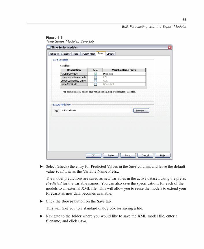
65


Figure 6-6Time Series Modeler, Save tab

E Select (check) the entry for Predicted Values in the Save column, and leave the defaultvalue Predicted as the Variable Name Prefix.

The model predictions are saved as new variables in the active dataset, using the prefixPredicted for the variable names. You can also save the specifications for each of themodels to an external XML file. This will allow you to reuse the models to extend yourforecasts as new data becomes available.

E Click the Browse button on the Save tab.

This will take you to a standard dialog box for saving a file.

E Navigate to the folder where you would like to save the XML model file, enter afilename, and click Save.

66

Chapter 6

The path to the XML model file should now appear on the Save tab.

E Click the Statistics tab.

Figure 6-7Time Series Modeler, Statistics tab

E Select Display forecasts.

This option produces a table of forecasted values for each dependent variable seriesand provides another option—other than saving the predictions as new variables—forobtaining these values.

The default selection of Goodness of fit (in the Statistics for Comparing Modelsgroup) produces a table with fit statistics—such as R-squared, mean absolutepercentage error, and normalized BIC—calculated across all of the models. It providesa concise summary of how well the models fit the data.

67


E Click the Plots tab.

Figure 6-8Time Series Modeler, Plots tab

E Deselect Series in the Plots for Individual Models group.

This suppresses the generation of series plots for each of the models. In this example,we are more interested in saving the forecasts as new variables than generating plots ofthe forecasts.

The Plots for Comparing Models group provides several plots (in the form ofhistograms) of fit statistics calculated across all models.

E Select Mean absolute percentage error and Maximum absolute percentage error in thePlots for Comparing Models group.

68

Chapter 6

Absolute percentage error is a measure of how much a dependent series varies from itsmodel-predicted level. By examining the mean and maximum across all models, youcan get an indication of the uncertainty in your predictions. And looking at summaryplots of percentage errors, rather than absolute errors, is advisable since the dependentseries represent subscriber numbers for markets of varying sizes.

E Click OK in the Time Series Modeler dialog box.

Model Summary ChartsFigure 6-9Histogram of mean absolute percentage error

This histogram displays the mean absolute percentage error (MAPE) across all models.It shows that all models display a mean uncertainty of roughly 1%.

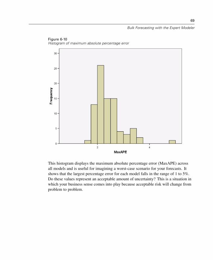
69


Figure 6-10Histogram of maximum absolute percentage error

This histogram displays the maximum absolute percentage error (MaxAPE) acrossall models and is useful for imagining a worst-case scenario for your forecasts. Itshows that the largest percentage error for each model falls in the range of 1 to 5%.Do these values represent an acceptable amount of uncertainty? This is a situation inwhich your business sense comes into play because acceptable risk will change fromproblem to problem.

70

Chapter 6

Model PredictionsFigure 6-11New variables containing model predictions

The Data Editor shows the new variables containing the model predictions. Althoughonly two are shown here, there are 85 new variables, one for each of the 85 dependentseries. The variable names consist of the default prefix Predicted, followed by thename of the associated dependent variable (for example, Market_1), followed by amodel identifier (for example, Model_1).

Three new cases, containing the forecasts for January 2004 through March 2004,have been added to the dataset, along with automatically generated date labels. Each ofthe new variables contains the model predictions for the estimation period (January1999 through December 2003), allowing you to see how well the model fits the knownvalues.

Figure 6-12Forecast table

71


You also chose to create a table with the forecasted values. The table consists of thepredicted values in the forecast period but—unlike the new variables containing themodel predictions—does not include predicted values in the estimation period. Theresults are organized by model and identified by the model name, which consistsof the name (or label) of the associated dependent variable followed by a modelidentifier—just like the names of the new variables containing the model predictions.The table also includes the upper confidence limits (UCL) and lower confidence limits(LCL) for the forecasted values (95% by default).

You have now seen two approaches for obtaining the forecasted values: saving theforecasts as new variables in the active dataset and creating a forecast table. With eitherapproach, you will have a number of options available for exporting your forecasts(for example, into an Excel spreadsheet).

Summary

You have learned how to use the Expert Modeler to produce forecasts for multipleseries, and you have saved the resulting models to an external XML file. In thenext example, you will learn how to extend your forecasts as new data becomesavailable—without having to rebuild your models—by using the Apply Time SeriesModels procedure.

Chapter

7Bulk Reforecasting by ApplyingSaved Models

You have used the Time Series Modeler to create models for your time series data andto produce initial forecasts based on available data. You plan to reuse these models toextend your forecasts as more current data becomes available, so you saved the modelsto an external file. You are now ready to apply the saved models.

This example is a natural extension of the previous one, “Bulk Forecasting with theExpert Modeler” in Chapter 6 on p. 59, but can also be used independently. In thisscenario, you are an analyst for a national broadband provider who is required toproduce monthly forecasts of user subscriptions for each of 85 local markets. You havealready used the Expert Modeler to create models and to forecast three months intothe future. Your data warehouse has been refreshed with actual data for the originalforecast period, so you would like to use that data to extend the forecast horizon byanother three months.

The updated monthly historical data is collected in broadband_2.sav, andthe saved models are in broadband_models.xml. Both files can be found in the\tutorial\sample_files\ folder where SPSS was installed. Of course, if you workedthrough the previous example and saved your own model file, you can use that oneinstead of broadband_models.xml.


To apply models:


Time SeriesApply Models...

73

74

Chapter 7

Figure 7-1Apply Time Series Models dialog box

E Click Browse, navigate to the \tutorial\sample_files\ folder where you installed SPSS,and select broadband_models.xml (or choose your own model file saved from theprevious example).

The path to broadband_models.xml (or your own model file) should now appear onthe Models tab.

E Select Reestimate from data.

75

Bulk Reforecasting by Applying Saved Models

To incorporate new values of your time series into forecasts, the Apply Time SeriesModels procedure will have to reestimate the model parameters. The structure of themodels remains the same though, so the computing time to reestimate is much quickerthan the original computing time to build the models.

The set of cases used for reestimation needs to include the new data. This will beassured if you use the default estimation period of First Case to Last Case. If you everneed to set the estimation period to something other than the default, you can do so byselecting Based on time or case range in the Select Cases dialog box.

E Select First case after end of estimation period through a specified date in the ForecastPeriod group.


The dataset contains data from January 1999 through March 2004. With the currentsettings, the forecast period will be April 2004 through June 2004.


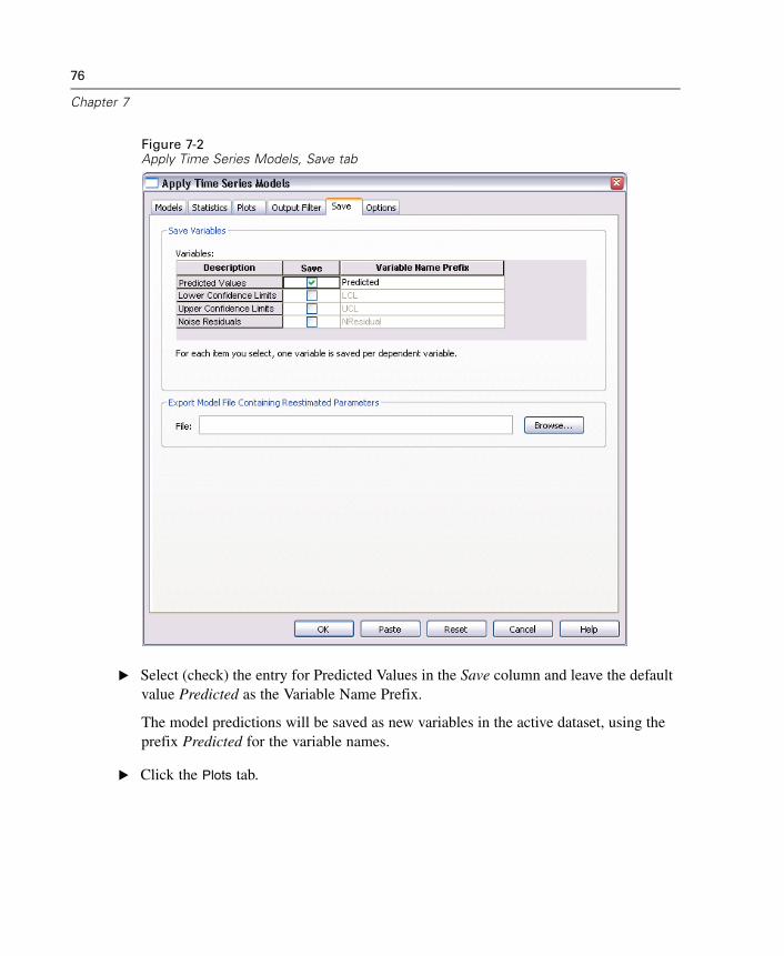
76

Chapter 7

Figure 7-2Apply Time Series Models, Save tab

E Select (check) the entry for Predicted Values in the Save column and leave the defaultvalue Predicted as the Variable Name Prefix.

The model predictions will be saved as new variables in the active dataset, using theprefix Predicted for the variable names.


77


Figure 7-3Apply Time Series Models, Plots tab

E Deselect Series in the Plots for Individual Models group.

This suppresses the generation of series plots for each of the models. In this example,we are more interested in saving the forecasts as new variables than generating plots ofthe forecasts.

E Click OK in the Apply Time Series Models dialog box.

78

Chapter 7

Model Fit StatisticsFigure 7-4Model Fit table

The Model Fit table provides fit statistics calculated across all of the models. Itprovides a concise summary of how well the models, with reestimated parameters, fitthe data. For each statistic, the table provides the mean, standard error (SE), minimum,and maximum value across all models. It also contains percentile values that provideinformation on the distribution of the statistic across models. For each percentile,that percentage of models have a value of the fit statistic below the stated value. Forinstance, 95% of the models have a value of MaxAPE (maximum absolute percentageerror) that is less than 3.676.

While a number of statistics are reported, we will focus on two: MAPE (meanabsolute percentage error) and MaxAPE (maximum absolute percentage error).Absolute percentage error is a measure of how much a dependent series variesfrom its model-predicted level and provides an indication of the uncertainty in yourpredictions. The mean absolute percentage error varies from a minimum of 0.669% toa maximum of 1.026% across all models. The maximum absolute percentage errorvaries from 1.742% to 4.373% across all models. So the mean uncertainty in eachmodel’s predictions is about 1% and the maximum uncertainty is around 2.5% (themean value of MaxAPE), with a worst case scenario of about 4%. Whether thesevalues represent an acceptable amount of uncertainty depends on the degree of riskyou are willing to accept.

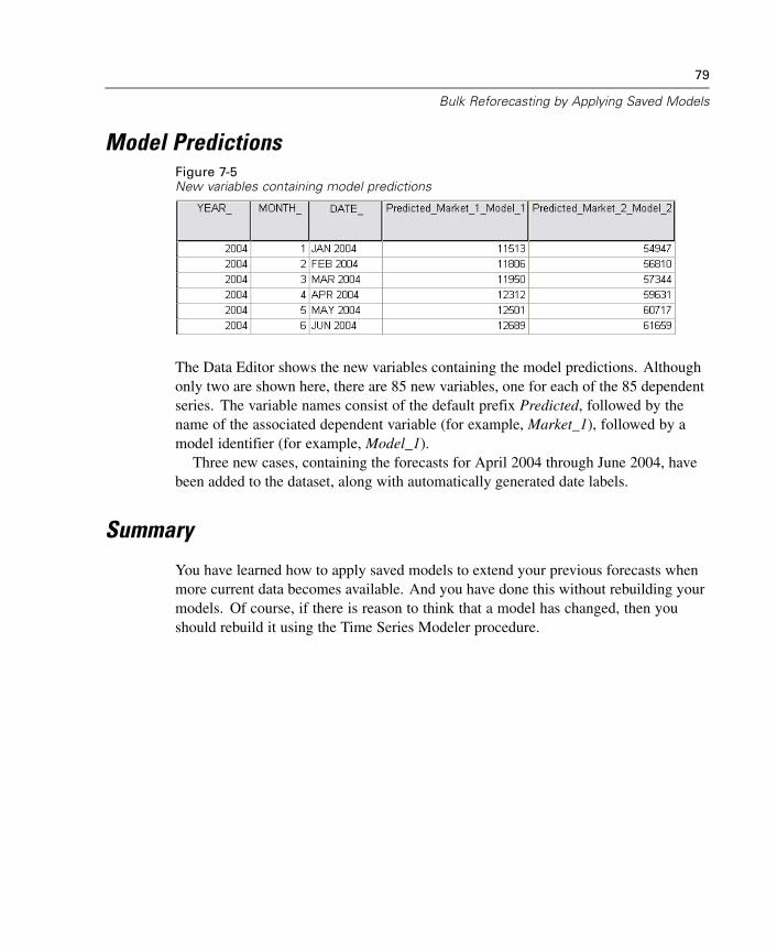
79


Model PredictionsFigure 7-5New variables containing model predictions

The Data Editor shows the new variables containing the model predictions. Althoughonly two are shown here, there are 85 new variables, one for each of the 85 dependentseries. The variable names consist of the default prefix Predicted, followed by thename of the associated dependent variable (for example, Market_1), followed by amodel identifier (for example, Model_1).

Three new cases, containing the forecasts for April 2004 through June 2004, havebeen added to the dataset, along with automatically generated date labels.

Summary

You have learned how to apply saved models to extend your previous forecasts whenmore current data becomes available. And you have done this without rebuilding yourmodels. Of course, if there is reason to think that a model has changed, then youshould rebuild it using the Time Series Modeler procedure.

Chapter

8Using the Expert Modeler toDetermine Significant Predictors

A catalog company, interested in developing a forecasting model, has collected dataon monthly sales of men’s clothing along with several series that might be usedto explain some of the variation in sales. Possible predictors include the number ofcatalogs mailed, the number of pages in the catalog, the number of phone lines openfor ordering, the amount spent on print advertising, and the number of customer servicerepresentatives. Are any of these predictors useful for forecasting?

In this example, you will use the Expert Modeler with all of the candidate predictorsto find the best model. Since the Expert Modeler only selects those predictors that havea statistically significant relationship with the dependent series, you will know whichpredictors are useful, and you will have a model for forecasting with them. Once youare finished, you might want to work through the next example, “Experimenting withPredictors by Applying Saved Models” in Chapter 9 on p. 93, which investigates theeffect on sales of different predictor scenarios using the model built in this example.

The data for the current example is collected in catalog_seasfac.sav, found in the\tutorial\sample_files\ folder where you installed SPSS.

Plotting Your Data

It is always a good idea to plot your data, especially if you are only working withone series:


Sequence...

81

82

Chapter 8


E Select Sales of Men’s Clothing and move it into the Variables list.

E Select Date (the one labeled DATE_) and move it into the Time Axis Labels box.

E Click OK.

83

Using the Expert Modeler to Determine Significant Predictors

Figure 8-2Sales of men’s clothing (in U.S. dollars)

The series exhibits numerous peaks, many of which appear to be equally spaced, aswell as a clear upward trend. The equally spaced peaks suggests the presence of aperiodic component to the time series. Given the seasonal nature of sales, with highstypically occurring during the holiday season, you should not be surprised to find anannual seasonal component to the data.

There are also peaks that do not appear to be part of the seasonal pattern and whichrepresent significant deviations from the neighboring data points. These points may beoutliers, which can and should be addressed by the Expert Modeler.

84

Chapter 8


To use the Expert Modeler:




E Select Sales of Men’s Clothing for the dependent variable.

E Select Number of Catalogs Mailed through Number of Customer ServiceRepresentatives for the independent variables.

85


E Verify that Expert Modeler is selected in the Method drop-down list. The ExpertModeler will automatically find the best-fitting seasonal or non-seasonal model forthe dependent variable series.

E Click Criteria and then click the Outliers tab.

Figure 8-4Expert Modeler Criteria dialog box, Outliers tab

E Select Detect outliers automatically and leave the default selections for the types ofoutliers to detect.

Our visual inspection of the data suggested that there may be outliers. With the currentchoices, the Expert Modeler will search for the most common outlier types andincorporate any outliers into the final model. Outlier detection can add significantlyto the computing time needed by the Expert Modeler, so it is a feature that should

86

Chapter 8

be used with some discretion, particularly when modeling many series at once. Bydefault, outliers are not detected.

E Click Continue.

E Click the Save tab on the Time Series Modeler dialog box.


You will want to save the estimated model to an external XML file so that you canexperiment with different values of the predictors—using the Apply Time SeriesModels procedure—without having to rebuild the model.

E Click the Browse button on the Save tab.

This will take you to a standard dialog box for saving a file.

87


E Navigate to the folder where you would like to save the XML model file, enter afilename, and click Save.

The path to the XML model file should now appear on the Save tab.


Figure 8-6Time Series Modeler, Statistics tab

E Select Parameter estimates.

This option produces a table displaying all of the parameters, including the significantpredictors, for the model chosen by the Expert Modeler.


88

Chapter 8

Figure 8-7Time Series Modeler, Plots tab

E Deselect Forecasts.

In the current example, we are only interested in determining the significant predictorsand building a model. We will not be doing any forecasting.

E Select Fit values.

This option displays the predicted values in the period used to estimate the model. Thisperiod is referred to as the estimation period, and it includes all cases in the activedataset for this example. These values provide an indication of how well the modelfits the observed values, so they are referred to as fit values. The resulting plot willconsist of both the observed values and the fit values.

E Click OK in the Time Series Modeler dialog box.

89


Series PlotFigure 8-8Predicted and observed values

The predicted values show good agreement with the observed values, indicating thatthe model has satisfactory predictive ability. Notice how well the model predicts theseasonal peaks. And it does a good job of capturing the upward trend of the data.

90

Chapter 8

Model Description TableFigure 8-9Model Description table

The model description table contains an entry for each estimated model and includesboth a model identifier and the model type. The model identifier consists of thename (or label) of the associated dependent variable and a system-assigned name.In the current example, the dependent variable is Sales of Men’s Clothing and thesystem-assigned name is Model_1.

The Time Series Modeler supports both exponential smoothing and ARIMAmodels. Exponential smoothing model types are listed by their commonly used namessuch as Holt and Winters’ Additive. ARIMA model types are listed using the standardnotation of ARIMA(p,d,q)(P,D,Q), where p is the order of autoregression, d is theorder of differencing (or integration), and q is the order of moving-average, and(P,D,Q) are their seasonal counterparts.

The Expert Modeler has determined that sales of men’s clothing is best described bya seasonal ARIMA model with one order of differencing. The seasonal nature of themodel accounts for the seasonal peaks that we saw in the series plot, and the singleorder of differencing reflects the upward trend that was evident in the data.

Model Statistics TableFigure 8-10Model Statistics table

The model statistics table provides summary information and goodness-of-fit statisticsfor each estimated model. Results for each model are labeled with the model identifierprovided in the model description table. First, notice that the model contains twopredictors out of the five candidate predictors that you originally specified. So itappears that the Expert Modeler has identified two independent variables that mayprove useful for forecasting.

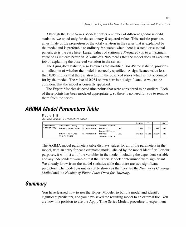
91


Although the Time Series Modeler offers a number of different goodness-of-fitstatistics, we opted only for the stationary R-squared value. This statistic providesan estimate of the proportion of the total variation in the series that is explained bythe model and is preferable to ordinary R-squared when there is a trend or seasonalpattern, as is the case here. Larger values of stationary R-squared (up to a maximumvalue of 1) indicate better fit. A value of 0.948 means that the model does an excellentjob of explaining the observed variation in the series.

The Ljung-Box statistic, also known as the modified Box-Pierce statistic, providesan indication of whether the model is correctly specified. A significance value lessthan 0.05 implies that there is structure in the observed series which is not accountedfor by the model. The value of 0.984 shown here is not significant, so we can beconfident that the model is correctly specified.

The Expert Modeler detected nine points that were considered to be outliers. Eachof these points has been modeled appropriately, so there is no need for you to removethem from the series.

ARIMA Model Parameters TableFigure 8-11ARIMA Model Parameters table

The ARIMA model parameters table displays values for all of the parameters in themodel, with an entry for each estimated model labeled by the model identifier. For ourpurposes, it will list all of the variables in the model, including the dependent variableand any independent variables that the Expert Modeler determined were significant.We already know from the model statistics table that there are two significantpredictors. The model parameters table shows us that they are the Number of CatalogsMailed and the Number of Phone Lines Open for Ordering.

SummaryYou have learned how to use the Expert Modeler to build a model and identifysignificant predictors, and you have saved the resulting model to an external file. Youare now in a position to use the Apply Time Series Models procedure to experiment

92

Chapter 8

with alternative scenarios for the predictor series and see how the alternatives affectthe sales forecasts.

Chapter

9Experimenting with Predictors byApplying Saved Models

You’ve used the Time Series Modeler to create a model for your data and to identifywhich predictors may prove useful for forecasting. The predictors represent factorsthat are within your control, so you’d like to experiment with their values in theforecast period to see how forecasts of the dependent variable are affected. This task iseasily accomplished with the Apply Time Series Models procedure, using the modelfile that is created with the Time Series Modeler procedure.

This example is a natural extension of the previous example, “Using the ExpertModeler to Determine Significant Predictors” in Chapter 8 on p. 81, but this examplecan also be used independently. The scenario involves a catalog company that hascollected data about monthly sales of men’s clothing from January 1989 throughDecember 1998, along with several series that are thought to be potentially useful aspredictors of future sales. The Expert Modeler has determined that only two of the fivecandidate predictors are significant: the number of catalogs mailed and the number ofphone lines open for ordering.

When planning your sales strategy for the next year, you have limited resources toprint catalogs and keep phone lines open for ordering. Your budget for the first threemonths of 1999 allows for either 2000 additional catalogs or 5 additional phone linesover your initial projections. Which choice will generate more sales revenue for thisthree-month period?

The data for this example are collected in catalog_seasfac.sav, andcatalog_model.xml contains the model of monthly sales that is built with the ExpertModeler. Both files can be found in the \tutorial\sample_files\ subdirectory ofthe directory in which you installed SPSS. Of course, if you worked through theprevious example and saved your own model file, you can use that file instead ofcatalog_model.xml.

93

94

Chapter 9

Extending the Predictor Series

When you’re creating forecasts for dependent series with predictors, each predictorseries needs to be extended through the forecast period. Unless you know preciselywhat the future values of the predictors will be, you’ll need to estimate them. You canthen modify the estimates to test different predictor scenarios. The initial projectionsare easily created by using the Expert Modeler.



95

Experimenting with Predictors by Applying Saved Models


E Select Number of Catalogs Mailed and Number of Phone Lines Open for Ordering forthe dependent variables.


96

Chapter 9


E In the Save column, select (check) the entry for Predicted Values, and leave the defaultvalue Predicted for the Variable Name Prefix.

E Click the Options tab.

97


Figure 9-3Time Series Modeler, Options tab

E In the Forecast Period group, select First case after end of estimation period through a

specified date.


The data set contains data from January 1989 through December 1998, so with thecurrent settings, the forecast period will be January 1999 through March 1999.

E Click OK.

98

Chapter 9

Figure 9-4New variables containing forecasts for predictor series

The Data Editor shows the new variables Predicted_mail_Model_1 andPredicted_phone_Model_2, containing the model predicted values for the number ofcatalogs mailed and the number of phone lines. To extend our predictor series, weonly need the values for January 1999 through March 1999, which amounts to cases121 through 123.

E Copy the values of these three cases from Predicted_mail_Model_1 and append themto the variable mail.

E Repeat this process for Predicted_phone_Model_2, copying the last three cases andappending them to the variable phone.

Figure 9-5Predictor series extended through the forecast period

The predictors have now been extended through the forecast period.

99


Modifying Predictor Values in the Forecast Period

Testing the two scenarios of mailing more catalogs or providing more phone linesrequires modifying the estimates for the predictors mail or phone, respectively.Because we’re only modifying the predictor values for three cases (months), it wouldbe easy to enter the new values directly into the appropriate cells of the Data Editor.For instructional purposes, we’ll use the Compute Variable dialog box. When you havemore than a few values to modify, you’ll probably find the Compute Variable dialogbox more convenient.

E From the menus choose:Transform

Compute...

100

Chapter 9

Figure 9-6Compute Variable dialog box

E Enter mail for the target variable.

E In the Numeric Expression text box, enter mail + 2000.

E Click If.

101


Figure 9-7Compute Variable If Cases dialog box

E Select Include if case satisfies condition.

E In the text box, enter $CASENUM > 120.

This will limit changes to the variable mail to the cases in the forecast period.

E Click Continue.

E Click OK in the Compute Variable dialog box, and click OK when asked whether youwant to change the existing variable.

This results in increasing the values for mail—the number of catalogs mailed—by2000 for each of the three months in the forecast period. You’ve now prepared the datato test the first scenario, and you are ready to run the analysis.

Running the AnalysisE From the menus choose:

AnalyzeTime Series

Apply Models...

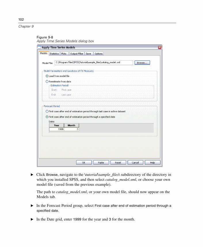
102

Chapter 9


E Click Browse, navigate to the \tutorial\sample_files\ subdirectory of the directory inwhich you installed SPSS, and then select catalog_model.xml, or choose your ownmodel file (saved from the previous example).

The path to catalog_model.xml, or your own model file, should now appear on theModels tab.

E In the Forecast Period group, select First case after end of estimation period through a

specified date.


103



Figure 9-9Apply Time Series Models, Statistics tab

E Select Display forecasts.

This results in a table of forecasted values for the dependent variable.


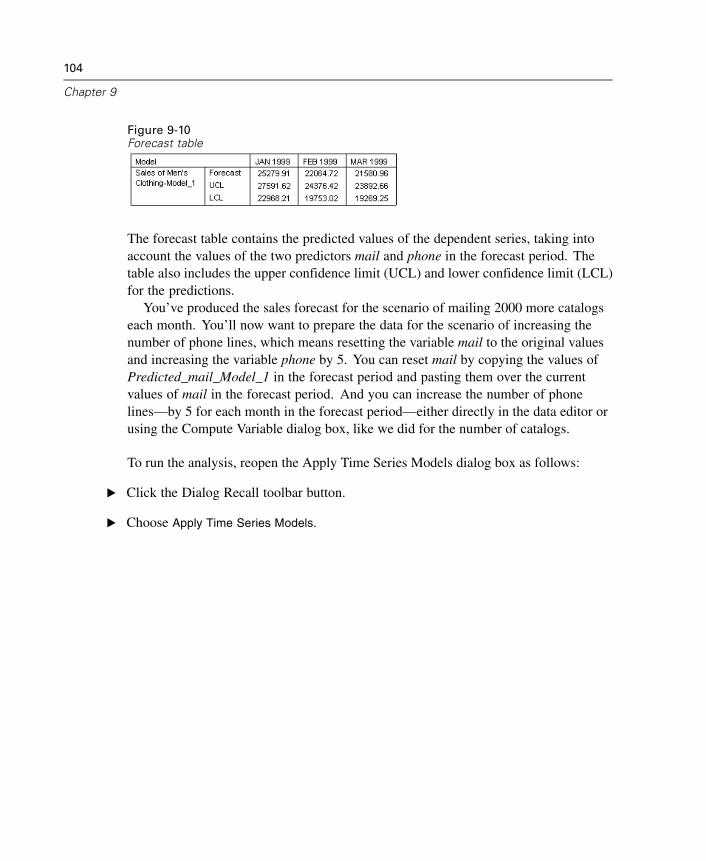
104

Chapter 9

Figure 9-10Forecast table

The forecast table contains the predicted values of the dependent series, taking intoaccount the values of the two predictors mail and phone in the forecast period. Thetable also includes the upper confidence limit (UCL) and lower confidence limit (LCL)for the predictions.

You’ve produced the sales forecast for the scenario of mailing 2000 more catalogseach month. You’ll now want to prepare the data for the scenario of increasing thenumber of phone lines, which means resetting the variable mail to the original valuesand increasing the variable phone by 5. You can reset mail by copying the values ofPredicted_mail_Model_1 in the forecast period and pasting them over the currentvalues of mail in the forecast period. And you can increase the number of phonelines—by 5 for each month in the forecast period—either directly in the data editor orusing the Compute Variable dialog box, like we did for the number of catalogs.

To run the analysis, reopen the Apply Time Series Models dialog box as follows:

E Click the Dialog Recall toolbar button.

E Choose Apply Time Series Models.

105




106

Chapter 9

Figure 9-12Forecast tables for the two scenarios

Displaying the forecast tables for both scenarios shows that, in each of the threeforecasted months, increasing the number of mailed catalogs is expected to generateapproximately $1500 more in sales than increasing the number of phone lines thatare open for ordering. Based on the analysis, it seems wise to allocate resources tothe mailing of 2000 additional catalogs.

Chapter

10Seasonal Decomposition

Removing Seasonality from Sales Data

A catalog company is interested in modeling the upward trend of sales of its men’sclothing line on a set of predictor variables (such as the number of catalogs mailedand the number of phone lines open for ordering). To this end, the company collectedmonthly sales of men’s clothing for a 10-year period. This information is collected incatalog.sav, which is found in the \tutorial\sample_files\ subdirectory of the directoryin which you installed SPSS.

To perform a trend analysis, you must remove any seasonal variations present in thedata. This task is easily accomplished with the Seasonal Decomposition procedure.

Preliminaries

In the examples that follow, it is more convenient to use variable names rather thanvariable labels.

E From the menus choose:Edit

Options...

107

108

Chapter 10

Figure 10-1Options dialog box

E Select Display names in the Variable Lists group.

E Click OK.

Determining and Setting the Periodicity

The Seasonal Decomposition procedure requires the presence of a periodic datecomponent in the active dataset—for example, a yearly periodicity of 12 (months),a weekly periodicity of 7 (days), and so on. It’s a good idea to plot your time seriesfirst, because viewing a time series plot often leads to a reasonable guess about theunderlying periodicity.

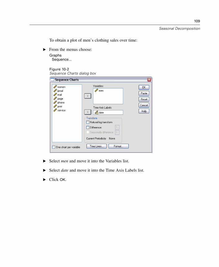
109


To obtain a plot of men’s clothing sales over time:


Sequence...


E Select men and move it into the Variables list.

E Select date and move it into the Time Axis Labels list.

E Click OK.

110

Chapter 10

Figure 10-3Sales of men’s clothing (in U.S. dollars)

The series exhibits a number of peaks, but they do not appear to be equally spaced.This output suggests that if the series has a periodic component, it also has fluctuationsthat are not periodic—the typical case for real-time series. Aside from the small-scalefluctuations, the significant peaks appear to be separated by more than a few months.Given the seasonal nature of sales, with typical highs during the December holidayseason, the time series probably has an annual periodicity. Also notice that the seasonalvariations appear to grow with the upward series trend, suggesting that the seasonalvariations may be proportional to the level of the series, which implies a multiplicativemodel rather than an additive model.

Examining the autocorrelations and partial autocorrelations of a time series provides amore quantitative conclusion about the underlying periodicity.


Time SeriesAutocorrelations...

111


Figure 10-4Autocorrelations dialog box


E Click OK.

Figure 10-5Autocorrelation plot for men

112

Chapter 10

The autocorrelation function shows a significant peak at a lag of 1 with a longexponential tail—a typical pattern for time series. The significant peak at a lag of 12suggests the presence of an annual seasonal component in the data. Examination of thepartial autocorrelation function will allow a more definitive conclusion.

Figure 10-6Partial autocorrelation plot for men

The significant peak at a lag of 12 in the partial autocorrelation function confirms thepresence of an annual seasonal component in the data.

To set an annual periodicity:

E From the menus choose:Data

Define Dates...

113


Figure 10-7Define Dates dialog box

E Select Years, months in the Cases Are list.

E Enter 1989 for the year and 1 for the month.

E Click OK.

This sets the periodicity to 12 and creates a set of date variables that are designed towork with Trends procedures.


To run the Seasonal Decomposition procedure:


Time SeriesSeasonal Decomposition...

114

Chapter 10

Figure 10-8Seasonal Decomposition dialog box


E Select Multiplicative in the Model group.

E Click OK.

Understanding the Output

The Seasonal Decomposition procedure creates four new variables for each of theoriginal variables analyzed by the procedure. By default, the new variables are added tothe active data set. The new series have names beginning with the following prefixes:

SAF. Seasonal adjustment factors, representing seasonal variation. For the multiplicativemodel, the value 1 represents the absence of seasonal variation; for the additive model,the value 0 represents the absence of seasonal variation.

SAS. Seasonally adjusted series, representing the original series with seasonalvariations removed. Working with a seasonally adjusted series, for example, allows atrend component to be isolated and analyzed independent of any seasonal component.

STC. Smoothed trend-cycle component, which is a smoothed version of the seasonallyadjusted series that shows both trend and cyclic components.

ERR. The residual component of the series for a particular observation.

115


For the present case, the seasonally adjusted series is the most appropriate, because itrepresents the original series with the seasonal variations removed.


To plot the seasonally adjusted series:

E Open the Sequence Charts dialog box.

E Click Reset to clear any previous selections, and then select SAS_1 and move it intothe Variables list.

E Click OK.

116

Chapter 10

Figure 10-10Seasonally adjusted series

The seasonally adjusted series shows a clear upward trend. A number of peaks areevident, but they appear at random intervals, showing no evidence of an annual pattern.

Summary

Using the Seasonal Decomposition procedure, you have removed the seasonalcomponent of a periodic time series to produce a series that is more suitable for trendanalysis. Examination of the autocorrelations and partial autocorrelations of the timeseries was useful in determining the underlying periodicity—in this case, annual.

117


Related Procedures

The Seasonal Decomposition procedure is useful for removing a single seasonalcomponent from a periodic time series.

To perform a more in-depth analysis of the periodicity of a time series than isprovided by the partial correlation function, use the Spectral Plots procedure.For more information, see Chapter 11.

Chapter

11Spectral Plots

Using Spectral Plots to Verify Expectations about Periodicity

Time series representing retail sales typically have an underlying annual periodicity,due to the usual peak in sales during the holiday season. Producing sales projectionsmeans building a model of the time series, which means identifying any periodiccomponents. A plot of the time series may not always uncover the annual periodicitybecause time series contain random fluctuations that often mask the underlyingstructure.

Monthly sales data for a catalog company are stored in catalog.sav, which is foundin the \tutorial\sample_files\ subdirectory of the directory in which you installed SPSS.Before proceeding with sales projections, you want to confirm that the sales dataexhibits an annual periodicity. A plot of the time series shows many peaks with anirregular spacing, so any underlying periodicity is not evident. Use the Spectral Plotsprocedure to identify any periodicity in the sales data.


To run the Spectral Plots procedure:


Time SeriesSpectral...

119

120

Chapter 11

Figure 11-1Spectral Plots dialog box

E Select Sales of Men’s Clothing and move it into the Variables list.

E Select Spectral density in the Plot group.

E Click OK.

121

Spectral Plots

Understanding the Periodogram and Spectral DensityFigure 11-2Periodogram

The plot of the periodogram shows a sequence of peaks that stand out from thebackground noise, with the lowest frequency peak at a frequency of just less than0.1. You suspect that the data contain an annual periodic component, so consider thecontribution that an annual component would make to the periodogram. Each of thedata points in the time series represents a month, so an annual periodicity correspondsto a period of 12 in the current data set. Because period and frequency are reciprocalsof each other, a period of 12 corresponds to a frequency of 1/12 (or 0.083). So anannual component implies a peak in the periodogram at 0.083, which seems consistentwith the presence of the peak just below a frequency of 0.1.

122

Chapter 11

Figure 11-3Univariate statistics table

The univariate statistics table contains the data points that are used to plot theperiodogram. Notice that, for frequencies of less than 0.1, the largest value in thePeriodogram column occurs at a frequency of 0.08333—precisely what you expectto find if there is an annual periodic component. This information confirms theidentification of the lowest frequency peak with an annual periodic component. Butwhat about the other peaks at higher frequencies?

123

Spectral Plots

Figure 11-4Spectral density

The remaining peaks are best analyzed with the spectral density function, which issimply a smoothed version of the periodogram. Smoothing provides a means ofeliminating the background noise from a periodogram, allowing the underlyingstructure to be more clearly isolated.

The spectral density consists of five distinct peaks that appear to be equally spaced.The lowest frequency peak simply represents the smoothed version of the peak at0.08333. To understand the significance of the four higher frequency peaks, rememberthat the periodogram is calculated by modeling the time series as the sum of cosine andsine functions. Periodic components that have the shape of a sine or cosine function(sinusoidal) show up in the periodogram as single peaks. Periodic components that arenot sinusoidal show up as a series of equally spaced peaks of different heights, withthe lowest frequency peak in the series occurring at the frequency of the periodiccomponent. So the four higher frequency peaks in the spectral density simply indicatethat the annual periodic component is not sinusoidal.

You have now accounted for all of the discernible structure in the spectral densityplot and conclude that the data contain a single periodic component with a periodof 12 months.

124

Chapter 11

Summary

Using the Spectral Plots procedure, you have confirmed the existence of an annualperiodic component of a time series, and you have verified that no other significantperiodicities are present. The spectral density was seen to be more useful than theperiodogram for uncovering the underlying structure, because the spectral densitysmoothes out the fluctuations that are caused by the nonperiodic component of the data.

Related Procedures

The Spectral Plots procedure is useful for identifying the periodic components ofa time series.

To remove a periodic component from a time series—for instance, to perform atrend analysis—use the Seasonal Decomposition procedure. See Chapter 10 fordetails.

Appendix

AGoodness-of-Fit Measures

This section provides definitions of the goodness-of-fit measures used in time seriesmodeling.

Stationary R-squared. A measure that compares the stationary part of the model to asimple mean model. This measure is preferable to ordinary R-squared when thereis a trend or seasonal pattern. Stationary R-squared can be negative with a range ofnegative infinity to 1. Negative values mean that the model under considerationis worse than the baseline model. Positive values mean that the model underconsideration is better than the baseline model.

R-squared. An estimate of the proportion of the total variation in the series that isexplained by the model. This measure is most useful when the series is stationary.R-squared can be negative with a range of negative infinity to 1. Negative valuesmean that the model under consideration is worse than the baseline model. Positivevalues mean that the model under consideration is better than the baseline model.

RMSE. Root Mean Square Error. The square root of mean square error. A measureof how much a dependent series varies from its model-predicted level, expressedin the same units as the dependent series.

MAPE. Mean Absolute Percentage Error. A measure of how much a dependentseries varies from its model-predicted level. It is independent of the units used andcan therefore be used to compare series with different units.

MAE. Mean absolute error. Measures how much the series varies from itsmodel-predicted level. MAE is reported in the original series units.

MaxAPE. Maximum Absolute Percentage Error. The largest forecasted error,expressed as a percentage. This measure is useful for imagining a worst-casescenario for your forecasts.

MaxAE. Maximum Absolute Error. The largest forecasted error, expressed in thesame units as the dependent series. Like MaxAPE, it is useful for imagining theworst-case scenario for your forecasts. Maximum absolute error and maximum

125

126

Appendix A

absolute percentage error may occur at different series points--for example, whenthe absolute error for a large series value is slightly larger than the absolute errorfor a small series value. In that case, the maximum absolute error will occur atthe larger series value and the maximum absolute percentage error will occur atthe smaller series value.

Normalized BIC. Normalized Bayesian Information Criterion. A general measureof the overall fit of a model that attempts to account for model complexity. It isa score based upon the mean square error and includes a penalty for the numberof parameters in the model and the length of the series. The penalty removes theadvantage of models with more parameters, making the statistic easy to compareacross different models for the same series.

Appendix

BOutlier Types

This section provides definitions of the outlier types used in time series modeling.

Additive. An outlier that affects a single observation. For example, a data codingerror might be identified as an additive outlier.

Level shift. An outlier that shifts all observations by a constant, starting at aparticular series point. A level shift could result from a change in policy.

Innovational. An outlier that acts as an addition to the noise term at a particularseries point. For stationary series, an innovational outlier affects severalobservations. For nonstationary series, it may affect every observation starting at aparticular series point.

Transient. An outlier whose impact decays exponentially to 0.

Seasonal additive. An outlier that affects a particular observation and allsubsequent observations separated from it by one or more seasonal periods. Allsuch observations are affected equally. A seasonal additive outlier might occur if,beginning in a certain year, sales are higher every January.

Local trend. An outlier that starts a local trend at a particular series point.

Additive patch. A group of two or more consecutive additive outliers. Selecting thisoutlier type results in the detection of individual additive outliers in addition topatches of them.

127

Appendix

CGuide to ACF/PACF Plots

The plots shown here are those of pure or theoretical ARIMA processes. Here aresome general guidelines for identifying the process:

Nonstationary series have an ACF that remains significant for half a dozen or morelags, rather than quickly declining to 0. You must difference such a series untilit is stationary before you can identify the process.

Autoregressive processes have an exponentially declining ACF and spikes in thefirst one or more lags of the PACF. The number of spikes indicates the order ofthe autoregression.

Moving average processes have spikes in the first one or more lags of the ACFand an exponentially declining PACF. The number of spikes indicates the orderof the moving average.

Mixed (ARMA) processes typically show exponential declines in both the ACFand the PACF.

At the identification stage, you do not need to worry about the sign of the ACF orPACF, or about the speed with which an exponentially declining ACF or PACFapproaches 0. These depend upon the sign and actual value of the AR and MAcoefficients. In some instances, an exponentially declining ACF alternates betweenpositive and negative values.

ACF and PACF plots from real data are never as clean as the plots shown here. Youmust learn to pick out what is essential in any given plot. Always check the ACF andPACF of the residuals, in case your identification is wrong. Bear in mind that:

Seasonal processes show these patterns at the seasonal lags (the multiples of theseasonal period).

129

130

Appendix C

You are entitled to treat nonsignificant values as 0. That is, you can ignorevalues that lie within the confidence intervals on the plots. You do not have toignore them, however, particularly if they continue the pattern of the statisticallysignificant values.

An occasional autocorrelation will be statistically significant by chance alone. Youcan ignore a statistically significant autocorrelation if it is isolated, preferably ata high lag, and if it does not occur at a seasonal lag.

Consult any text on ARIMA analysis for a more complete discussion of ACF andPACF plots.

ARIMA(0,0,1), θ>0

ACF PACF

131

Guide to ACF/PACF Plots

ARIMA(0,0,1), θ<0

ACF PACF

ARIMA(0,0,2), θ1θ2>0

ACF PACF

132

Appendix C

ARIMA(1,0,0), φ>0

ACF PACF

ARIMA(1,0,0), φ<0

ACF PACF

133

Guide to ACF/PACF Plots

ARIMA(1,0,1), φ<0, θ>0

ACF PACF

ARIMA(2,0,0), φ1φ2>0

ACF PACF

134

Appendix C

ARIMA(0,1,0) (integrated series)

ACF

Bibliography

Box, G. E. P., G. M. Jenkins, and G. C. Reinsel. 1994. Time series analysis:Forecasting and control, 3rd ed. Englewood Cliffs, N.J.: Prentice Hall.

Gardner, E. S. 1985. Exponential smoothing: The state of the art. Journal ofForecasting, 4, 1–28.

Pena, D., G. C. Tiao, and R. S. Tsay, eds. 2001. A course in time series analysis.New York: John Wiley and Sons.

135

Index

ACF

in Apply Time Series Models, 38, 41in Time Series Modeler, 22, 24plots for pure ARIMA processes, 129

additive outlier, 127in Time Series Modeler, 12, 20

additive patch outlier, 127in Time Series Modeler, 12, 20

Apply Time Series Models, 33, 73, 93best- and poorest-fitting models, 43Box-Ljung statistic, 38confidence intervals, 41, 47estimation period, 36fit values, 41forecast period, 36, 75, 102forecast table, 104forecasts, 38, 41, 103goodness-of-fit statistics, 38, 41, 78missing values, 47model fit table, 78model parameters, 38new variable names, 45, 79reestimate model parameters, 36, 74residual autocorrelation function, 38, 41residual partial autocorrelation function, 38, 41saving predictions, 45, 76saving reestimated models in XML, 45statistics across all models, 38, 41, 78

ARIMA model parameters table

in Time Series Modeler, 91ARIMA models, 8, 16

autoregressive orders, 16

constant, 16differencing orders, 16moving average orders, 16outliers, 20seasonal orders, 16transfer functions, 18

autocorrelation function


autoregression

ARIMA models, 16

Box-Ljung statistic

in Apply Time Series Models, 38in Time Series Modeler, 22, 91

Brown’s exponential smoothing model, 13

confidence intervals

in Apply Time Series Models, 41, 47in Time Series Modeler, 24, 30

damped exponential smoothing model, 13difference transformation

ARIMA models, 16

estimation period, 3in Apply Time Series Models, 36in Time Series Modeler, 9, 62

events, 11in Time Series Modeler, 10

137

138

Index

Expert Modeler, 8, 59limiting the model space, 10, 63outliers, 12, 85

exponential smoothing models, 8, 13

fit values


forecast period

in Apply Time Series Models, 36, 75, 102in Time Series Modeler, 9, 30, 62, 64

forecast table

in Apply Time Series Models, 104in Time Series Modeler, 70

forecasts

in Apply Time Series Models, 38, 41, 103in Time Series Modeler, 22, 24, 66

goodness of fit

definitions, 125in Apply Time Series Models, 38, 41, 78in Time Series Modeler, 22, 24, 66

harmonic analysis, 53historical data


historical period, 3holdout cases, 3Holt’s exponential smoothing model, 13

innovational outlier, 127in Time Series Modeler, 12, 20

integration

ARIMA models, 16

level shift outlier, 127in Time Series Modeler, 12, 20

local trend outlier, 127in Time Series Modeler, 12, 20

log transformation

in Time Series Modeler, 13, 16, 18

MAE, 125in Apply Time Series Models, 38, 41in Time Series Modeler, 22, 24

MAPE, 125in Apply Time Series Models, 38, 41, 78in Time Series Modeler, 22, 24, 67

MaxAE, 125in Apply Time Series Models, 38, 41in Time Series Modeler, 22, 24

MaxAPE, 125in Apply Time Series Models, 38, 41, 78in Time Series Modeler, 22, 24, 67

maximum absolute error, 125in Apply Time Series Models, 38, 41in Time Series Modeler, 22, 24

maximum absolute percentage error, 125in Apply Time Series Models, 38, 41, 78in Time Series Modeler, 22, 24, 67

mean absolute error, 125in Apply Time Series Models, 38, 41in Time Series Modeler, 22, 24

mean absolute percentage error, 125in Apply Time Series Models, 38, 41, 78in Time Series Modeler, 22, 24, 67

missing values


model description table

in Time Series Modeler, 90

139

Index

model fit table

in Apply Time Series Models, 78model names

in Time Series Modeler, 30model parameters


model statistics table

in Time Series Modeler, 90models

ARIMA, 8, 16Expert Modeler, 8exponential smoothing, 8, 13

moving average

ARIMA models, 16

natural log transformation

in Time Series Modeler, 13, 16, 18normalized BIC (Bayesian information criterion),125


outliers

ARIMA models, 20definitions, 127Expert Modeler, 12, 85

PACF


partial autocorrelation function


periodicity

in Time Series Modeler, 10, 13, 16, 18

R2, 125in Apply Time Series Models, 38, 41in Time Series Modeler, 22, 24

reestimate model parameters

in Apply Time Series Models, 36, 74residuals


RMSE, 125in Apply Time Series Models, 38, 41in Time Series Modeler, 22, 24

root mean square error, 125in Apply Time Series Models, 38, 41in Time Series Modeler, 22, 24

save

model predictions, 28, 45model specifications in XML, 28new variable names, 28, 45reestimated models in XML, 45

seasonal additive outlier, 127in Time Series Modeler, 12, 20

Seasonal Decomposition, 49, 51–52assumptions, 49computing moving averages, 49create variables, 51models, 49new variables, 114periodic date component, 108related procedures, 117saving new variables, 51

seasonal difference transformation

ARIMA models, 16

140

Index

seasonal orders

ARIMA models, 16simple exponential smoothing model, 13simple seasonal exponential smoothing model, 13Spectral Plots, 53, 56

assumptions, 53bivariate spectral analysis, 55centering transformation, 55periodogram, 121related procedures, 124spectral density, 121spectral windows, 54

square root transformation

in Time Series Modeler, 13, 16, 18stationary R2, 125

in Apply Time Series Models, 38, 41in Time Series Modeler, 22, 24, 90

Time Series Modeler, 5ARIMA, 8, 16ARIMA model parameters table, 91best- and poorest-fitting models, 26Box-Ljung statistic, 22confidence intervals, 24, 30estimation period, 9, 62events, 10Expert Modeler, 8, 59, 81exponential smoothing, 8, 13fit values, 24, 88forecast period, 9, 30, 62, 64forecast table, 70forecasts, 22, 24, 66goodness-of-fit statistics, 22, 24, 66, 90missing values, 30model description table, 90model names, 30model parameters, 22, 87

model statistics table, 90new variable names, 28, 70outliers, 12, 20, 85periodicity, 10, 13, 16, 18residual autocorrelation function, 22, 24residual partial autocorrelation function, 22, 24saving model specifications in XML, 28, 65, 86saving predictions, 28, 65series transformation, 13, 16, 18statistics across all models, 22, 24, 66, 68transfer functions, 18

transfer functions, 18delay, 18denominator orders, 18difference orders, 18numerator orders, 18seasonal orders, 18

transient outlier, 127in Time Series Modeler, 12, 20

validation period, 3variable names


Winters’ exponential smoothing model

additive, 13multiplicative, 13

XML

saving reestimated models in XML, 45saving time series models in XML, 28, 65, 86

SPSS Trends™ 14 - Kuwait University Trends 14.0.pdf · Training Seminars SPSS Inc. provides both...

Documents

Transcript of SPSS Trends™ 14 - Kuwait University Trends 14.0.pdf · Training Seminars SPSS Inc. provides both...