SPSS Neural Network 16.0
107
SPSS Neural Networks ™ 16.0
-
Upload
tanu-priya -
Category
Documents
-
view
243 -
download
0
Transcript of SPSS Neural Network 16.0

8/8/2019 SPSS Neural Network 16.0
http://slidepdf.com/reader/full/spss-neural-network-160 1/107
SPSS Neural Networks™
16.0

8/8/2019 SPSS Neural Network 16.0
http://slidepdf.com/reader/full/spss-neural-network-160 2/107
For more information about SPSS® software products, please visit our Web site at http://www.spss.com or contact
SPSS Inc.
233 South Wacker Drive, 11th Floor
Chicago, IL 60606-6412
Tel: (312) 651-3000
Fax: (312) 651-3668
SPSS is a registered trademark and the other product names are the trademarks of SPSS Inc. for its proprietary computer
software. No material describing such software may be produced or distributed without the written permission of the owners of
the trademark and license rights in the software and the copyrights in the published materials.
The SOFTWARE and documentation are provided with RESTRICTED RIGHTS. Use, duplication, or disclosure by the
Government is subject to restrictions as set forth in subdivision (c) (1) (ii) of The Rights in Technical Data and Computer Software
clause at 52.227-7013. Contractor/manufacturer is SPSS Inc., 233 South Wacker Drive, 11th Floor, Chicago, IL 60606-6412.
Patent No. 7,023,453
General notice: Other product names mentioned herein are used for identification purposes only and may be trademarks of
their respective companies.
Windows is a registered trademark of Microsoft Corporation.
Apple, Mac, and the Mac logo are trademarks of Apple Computer, Inc., registered in the U.S. and other countries.
This product uses WinWrap Basic, Copyright 1993-2007, Polar Engineering and Consulting, http://www.winwrap.com.
SPSS Neural Networks™ 16.0
Copyright © 2007 by SPSS Inc.
All rights reserved.
Printed in the United States of America.
No part of this publication may be reproduced, stored in a retrieval system, or transmitted, in any form or by any means,
electronic, mechanical, photocopying, recording, or otherwise, without the prior written permission of the publisher.
ISBN-13: 978-1-56827-393-8
ISBN-10: 1-56827-393-2
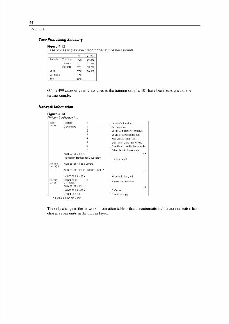
1 2 3 4 5 6 7 8 9 0 10 09 08 07
8/8/2019 SPSS Neural Network 16.0
http://slidepdf.com/reader/full/spss-neural-network-160 3/107
8/8/2019 SPSS Neural Network 16.0
http://slidepdf.com/reader/full/spss-neural-network-160 4/107
site at http://www.spss.com, or contact your local of fice, listed on the SPSS Web site at
http://www.spss.com/worldwide. Be prepared to identify yourself, your organization, and the
serial number of your system.
Additional Publications
Additional copies of product manuals may be purchased directly from SPSS Inc. Visit the SPSS
Web Store at http://www.spss.com/estore, or contact your local SPSS of fice, listed on the SPSS
Web site at http://www.spss.com/worldwide. For telephone orders in the United States and
Canada, call SPSS Inc. at 800-543-2185. For telephone orders outside of North America, contact
your local of fice, listed on the SPSS Web site.
The SPSS Statistical Procedures Companion, by Marija Norušis, has been published by
Prentice Hall. A new version of this book, updated for SPSS 16.0, is planned. The SPSS
Advanced Statistical Procedures Companion, also based on SPSS 16.0, is forthcoming. The
SPSS Guide to Data Analysis for SPSS 16.0 is also in development. Announcements of
publications available exclusively through Prentice Hall will be available on the SPSS Web site at
http://www.spss.com/estore (select your home country, and then click Books).
Tell Us Your Thoughts
Your comments are important. Please let us know about your experiences with SPSS products.
We especially like to hear about new and interesting applications using the SPSS Neural
Networks add-on module. Please send e-mail to [email protected] or write to SPSS Inc., Attn.:
Director of Product Planning, 233 South Wacker Drive, 11th Floor, Chicago, IL 60606-6412.
About This Manual
This manual documents the graphical user interface for the procedures included in the SPSS Neural Networks add-on module. Illustrations of dialog boxes are taken from SPSS. Detailed
information about the command syntax for features in the SPSS Neural Networks add-on module
is available in two forms: integrated into the overall Help system and as a separate document in
PDF form in the SPSS 16.0 Command Syntax Reference, available from the Help menu.
Contacting SPSS
If you would like to be on our mailing list, contact one of our of fices, listed on our Web site
at http://www.spss.com/worldwide.
iv

8/8/2019 SPSS Neural Network 16.0
http://slidepdf.com/reader/full/spss-neural-network-160 5/107
Contents
Part I: User’s Guide
1 Introduction to SPSS Neural Networks 1
What Is a Neural Network?. . . . . . . . . . . . . . . . . . . . . . . . . . . . . . . . . . . . . . . . . . . . . . . . . . . . . . 1
Neural Network Structure . . . . . . . . . . . . . . . . . . . . . . . . . . . . . . . . . . . . . . . . . . . . . . . . . . . . . . 2
2 Multilayer Perceptron 4
Partitions . . . . . . . . . . . . . . . . . . . . . . . . . . . . . . . . . . . . . . . . . . . . . . . . . . . . . . . . . . . . . . . . . . . 8
Architecture . . . . . . . . . . . . . . . . . . . . . . . . . . . . . . . . . . . . . . . . . . . . . . . . . . . . . . . . . . . . . . . . 9
Training . . . . . . . . . . . . . . . . . . . . . . . . . . . . . . . . . . . . . . . . . . . . . . . . . . . . . . . . . . . . . . . . . . . . 12
Output . . . . . . . . . . . . . . . . . . . . . . . . . . . . . . . . . . . . . . . . . . . . . . . . . . . . . . . . . . . . . . . . . . . . . 14
Save . . . . . . . . . . . . . . . . . . . . . . . . . . . . . . . . . . . . . . . . . . . . . . . . . . . . . . . . . . . . . . . . . . . . . . 17
Export . . . . . . . . . . . . . . . . . . . . . . . . . . . . . . . . . . . . . . . . . . . . . . . . . . . . . . . . . . . . . . . . . . . . . 19
Options . . . . . . . . . . . . . . . . . . . . . . . . . . . . . . . . . . . . . . . . . . . . . . . . . . . . . . . . . . . . . . . . . . . . 20
3 Radial Basis Function 22
Partitions . . . . . . . . . . . . . . . . . . . . . . . . . . . . . . . . . . . . . . . . . . . . . . . . . . . . . . . . . . . . . . . . . . . 25
Architecture . . . . . . . . . . . . . . . . . . . . . . . . . . . . . . . . . . . . . . . . . . . . . . . . . . . . . . . . . . . . . . . . 26
Output . . . . . . . . . . . . . . . . . . . . . . . . . . . . . . . . . . . . . . . . . . . . . . . . . . . . . . . . . . . . . . . . . . . . . 28
Save . . . . . . . . . . . . . . . . . . . . . . . . . . . . . . . . . . . . . . . . . . . . . . . . . . . . . . . . . . . . . . . . . . . . . . 30
Export . . . . . . . . . . . . . . . . . . . . . . . . . . . . . . . . . . . . . . . . . . . . . . . . . . . . . . . . . . . . . . . . . . . . . 32
Options . . . . . . . . . . . . . . . . . . . . . . . . . . . . . . . . . . . . . . . . . . . . . . . . . . . . . . . . . . . . . . . . . . . . 33
v
8/8/2019 SPSS Neural Network 16.0
http://slidepdf.com/reader/full/spss-neural-network-160 6/107
Part II: Examples
4 Multilayer Perceptron 35
Using a Multilayer Perceptron to Assess Credit Risk. . . . . . . . . . . . . . . . . . . . . . . . . . . . . . . . . . . 35
Preparing the Data for Analysis . . . . . . . . . . . . . . . . . . . . . . . . . . . . . . . . . . . . . . . . . . . . . . . 35
Running the Analysis . . . . . . . . . . . . . . . . . . . . . . . . . . . . . . . . . . . . . . . . . . . . . . . . . . . . . . . 38
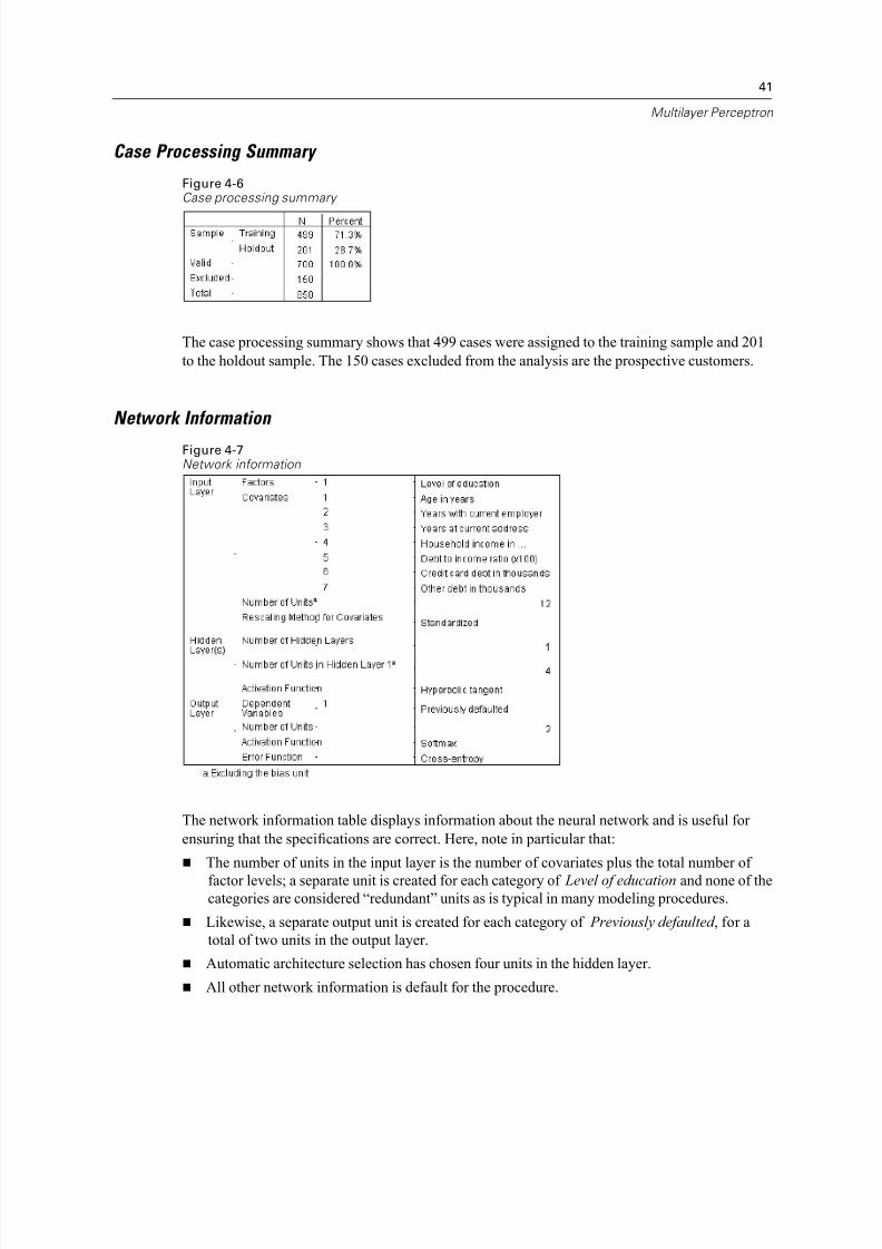
Case Processing Summary . . . . . . . . . . . . . . . . . . . . . . . . . . . . . . . . . . . . . . . . . . . . . . . . . . 41
Network Information . . . . . . . . . . . . . . . . . . . . . . . . . . . . . . . . . . . . . . . . . . . . . . . . . . . . . . . 41
Model Summary . . . . . . . . . . . . . . . . . . . . . . . . . . . . . . . . . . . . . . . . . . . . . . . . . . . . . . . . . . 42
Classification. . . . . . . . . . . . . . . . . . . . . . . . . . . . . . . . . . . . . . . . . . . . . . . . . . . . . . . . . . . . . 42
Correcting Overtraining . . . . . . . . . . . . . . . . . . . . . . . . . . . . . . . . . . . . . . . . . . . . . . . . . . . . . 43
Summary . . . . . . . . . . . . . . . . . . . . . . . . . . . . . . . . . . . . . . . . . . . . . . . . . . . . . . . . . . . . . . . . 53
Using a Multilayer Perceptron to Estimate Healthcare Costs and Lengths of Stay . . . . . . . . . . . . . 54
Preparing the Data for Analysis . . . . . . . . . . . . . . . . . . . . . . . . . . . . . . . . . . . . . . . . . . . . . . . 54
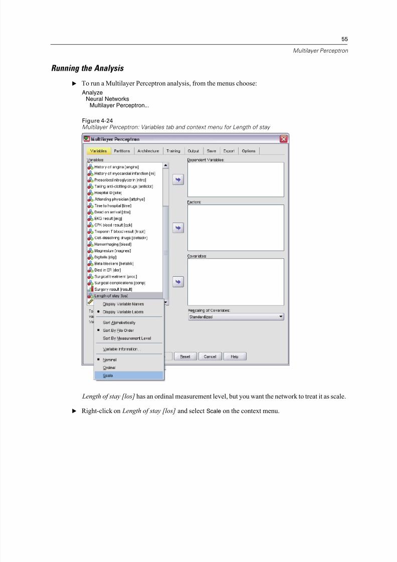
Running the Analysis . . . . . . . . . . . . . . . . . . . . . . . . . . . . . . . . . . . . . . . . . . . . . . . . . . . . . . . 55
Warnings. . . . . . . . . . . . . . . . . . . . . . . . . . . . . . . . . . . . . . . . . . . . . . . . . . . . . . . . . . . . . . . . 61
Case Processing Summary . . . . . . . . . . . . . . . . . . . . . . . . . . . . . . . . . . . . . . . . . . . . . . . . . . 62
Network Information . . . . . . . . . . . . . . . . . . . . . . . . . . . . . . . . . . . . . . . . . . . . . . . . . . . . . . . 63
Model Summary . . . . . . . . . . . . . . . . . . . . . . . . . . . . . . . . . . . . . . . . . . . . . . . . . . . . . . . . . . 64
Predicted-by-Observed Charts. . . . . . . . . . . . . . . . . . . . . . . . . . . . . . . . . . . . . . . . . . . . . . . . 65
Residual-by-Predicted Charts . . . . . . . . . . . . . . . . . . . . . . . . . . . . . . . . . . . . . . . . . . . . . . . . 67
Independent Variable Importance . . . . . . . . . . . . . . . . . . . . . . . . . . . . . . . . . . . . . . . . . . . . . 69
Summary . . . . . . . . . . . . . . . . . . . . . . . . . . . . . . . . . . . . . . . . . . . . . . . . . . . . . . . . . . . . . . . . 69
Recommended Readings . . . . . . . . . . . . . . . . . . . . . . . . . . . . . . . . . . . . . . . . . . . . . . . . . . . . . . . 70
5 Radial Basis Function 71
Using Radial Basis Function to Classify Telecommunications Customers. . . . . . . . . . . . . . . . . . . . 71
Preparing the Data for Analysis . . . . . . . . . . . . . . . . . . . . . . . . . . . . . . . . . . . . . . . . . . . . . . . 71
Running the Analysis . . . . . . . . . . . . . . . . . . . . . . . . . . . . . . . . . . . . . . . . . . . . . . . . . . . . . . . 72
Case Processing Summary . . . . . . . . . . . . . . . . . . . . . . . . . . . . . . . . . . . . . . . . . . . . . . . . . . 76
Network Information . . . . . . . . . . . . . . . . . . . . . . . . . . . . . . . . . . . . . . . . . . . . . . . . . . . . . . . 77
Model Summary . . . . . . . . . . . . . . . . . . . . . . . . . . . . . . . . . . . . . . . . . . . . . . . . . . . . . . . . . . 78
Classification. . . . . . . . . . . . . . . . . . . . . . . . . . . . . . . . . . . . . . . . . . . . . . . . . . . . . . . . . . . . . 78Predicted-by-Observed Chart . . . . . . . . . . . . . . . . . . . . . . . . . . . . . . . . . . . . . . . . . . . . . . . . 79
ROC Curve. . . . . . . . . . . . . . . . . . . . . . . . . . . . . . . . . . . . . . . . . . . . . . . . . . . . . . . . . . . . . . . 80
Cumulative Gains and Lift Charts . . . . . . . . . . . . . . . . . . . . . . . . . . . . . . . . . . . . . . . . . . . . . . 81
Recommended Readings . . . . . . . . . . . . . . . . . . . . . . . . . . . . . . . . . . . . . . . . . . . . . . . . . . . . . . . 83
vi

8/8/2019 SPSS Neural Network 16.0
http://slidepdf.com/reader/full/spss-neural-network-160 7/107
Appendix
A Sample Files 84
Bibliography 94
Index 96
vii

8/8/2019 SPSS Neural Network 16.0
http://slidepdf.com/reader/full/spss-neural-network-160 8/107

8/8/2019 SPSS Neural Network 16.0
http://slidepdf.com/reader/full/spss-neural-network-160 9/107
Part I: User’s Guide

8/8/2019 SPSS Neural Network 16.0
http://slidepdf.com/reader/full/spss-neural-network-160 10/107
8/8/2019 SPSS Neural Network 16.0
http://slidepdf.com/reader/full/spss-neural-network-160 11/107
Chapter
1
Introduction to SPSS Neural Networks
Neural networks are the preferred tool for many predictive data mining applications because of
their power, flexibility, and ease of use. Predictive neural networks are particularly useful in
applications where the underlying process is complex, such as:
Forecasting consumer demand to streamline production and delivery costs.
Predicting the probability of response to direct mail marketing to determine which households
on a mailing list should be sent an offer. Scoring an applicant to determine the risk of extending credit to the applicant.
Detecting fraudulent transactions in an insurance claims database.
Neural networks used in predictive applications, such as the multilayer perceptron (MLP) and
radial basis function (RBF) networks, are supervised in the sense that the model-predicted
results can be compared against known values of the target variables. The SPSS Neural Networks
option allows you to fit MLP and RBF networks and save the resulting models for scoring.
What Is a Neural Network?
The term neural network applies to a loosely related family of models, characterized by a large parameter space and flexible structure, descending from studies of brain functioning. As the
family grew, most of the new models were designed for nonbiological applications, though much
of the associated terminology reflects its origin.
Specific definitions of neural networks are as varied as the fields in which they are used. While
no single definition properly covers the entire family of models, for now, consider the following
description (Haykin, 1998):
A neural networ k is a massively parallel distributed processor that has a natural propensity for
storing experiential knowledge and making it available for use. It resembles the brain in two
respects:
Knowledge is acquired by the network through a learning process.
Interneuron connection strengths known as synaptic weights are used to store the knowledge.
For a discussion of why this definition is perhaps too restrictive, see (Ripley, 1996).
In order to differentiate neural networks from traditional statistical methods using this definition,
what is not said is just as significant as the actual text of the definition. For example, the traditional
linear regression model can acquire knowledge through the least-squares method and store that
knowledge in the regression coef ficients. In this sense, it is a neural network. In fact, you can
1

8/8/2019 SPSS Neural Network 16.0
http://slidepdf.com/reader/full/spss-neural-network-160 12/107
2
Chapter 1
argue that linear regression is a special case of certain neural networks. However, linear regression
has a rigid model structure and set of assumptions that are imposed before learning from the data.
By contrast, the definition above makes minimal demands on model structure and assumptions.
Thus, a neural network can approximate a wide range of statistical models without requiring
that you hypothesize in advance certain relationships between the dependent and independent
variables. Instead, the form of the relationships is determined during the learning process. If a
linear relationship between the dependent and independent variables is appropriate, the results
of the neural network should closely approximate those of the linear regression model. If a
nonlinear relationship is more appropriate, the neural network will automatically approximate the
“correct” model structure.
The trade-off for this flexibility is that the synaptic weights of a neural network are not
easily interpretable. Thus, if you are trying to explain an underlying process that produces the
relationships between the dependent and independent variables, it would be better to use a more
traditional statistical model. However, if model interpretability is not important, you can often
obtain good model results more quickly using a neural network.
Neural Network Structure
Although neural networks impose minimal demands on model structure and assumptions, it is
useful to understand the general network architecture. The multilayer perceptron (MLP) or
radial basis function (RBF) network is a function of predictors (also called inputs or independent
variables) that minimize the prediction error of target variables (also called outputs).
Consider the bankloan.sav dataset that ships with the product, in which you want to be able to
identify possible defaulters among a pool of loan applicants. An MLP or RBF network applied to
this problem is a function of the measurements that minimize the error in predicting default. The
following figure is useful for relating the form of this function.

8/8/2019 SPSS Neural Network 16.0
http://slidepdf.com/reader/full/spss-neural-network-160 13/107
3
Introduction to SPSS Neural Networks
Figure 1-1Feedforward architecture with one hidden layer
This structure is known as a feedforward architecture because the connections in the network
flow forward from the input layer to the output layer without any feedback loops. In this figure:
The input layer contains the predictors.
The hidden layer contains unobservable nodes, or units. The value of each hidden unit is
some function of the predictors; the exact form of the function depends in part upon the
network type and in part upon user-controllable specifications.
The output layer contains the responses. Since the history of default is a categorical variable
with two categories, it is recoded as two indicator variables. Each output unit is some function
of the hidden units. Again, the exact form of the function depends in part on the network type
and in part on user-controllable specifications.
The MLP network allows a second hidden layer; in that case, each unit of the second hidden layer
is a function of the units in the first hidden layer, and each response is a function of the units
in the second hidden layer.

8/8/2019 SPSS Neural Network 16.0
http://slidepdf.com/reader/full/spss-neural-network-160 14/107
Chapter
2Multilayer Perceptron
The Multilayer Perceptron (MLP) procedure produces a predictive model for one or more
dependent (target) variables based on the values of the predictor variables.
Examples. Following are two scenarios using the MLP procedure:
A loan of ficer at a bank needs to be able to identify characteristics that are indicative of people
who are likely to default on loans and use those characteristics to identify good and bad credit
risks. Using a sample of past customers, she can train a multilayer perceptron, validate the analysis
using a holdout sample of past customers, and then use the network to classify prospective
customers as good or bad credit risks.
A hospital system is interested in tracking costs and lengths of stay for patients admitted for
treatment of myocardial infarction (MI, or “heart attack”). Obtaining accurate estimates of these
measures allows the administration to properly manage the available bed space as patients are
treated. Using the treatment records of a sample of patients who received treatment for MI, the
administrator can train a network to predict both cost and length of stay.
Dependent variables. The dependent variables can be:
Nominal. A variable can be treated as nominal when its values represent categories with nointrinsic ranking (for example, the department of the company in which an employee works).
Examples of nominal variables include region, zip code, and religious af filiation.
Ordinal. A variable can be treated as ordinal when its values represent categories with some
intrinsic ranking (for example, levels of service satisfaction from highly dissatisfied to
highly satisfied). Examples of ordinal variables include attitude scores representing degree
of satisfaction or confidence and preference rating scores.
Scale. A variable can be treated as scale when its values represent ordered categories with a
meaningful metric, so that distance comparisons between values are appropriate. Examples of
scale variables include age in years and income in thousands of dollars.
The procedure assumes that the appropriate measurement level has been assigned to all
dependent variables; however, you can temporarily change the measurement level for a
variable by right-clicking the variable in the source variable list and selecting a measurement
level from the context menu.
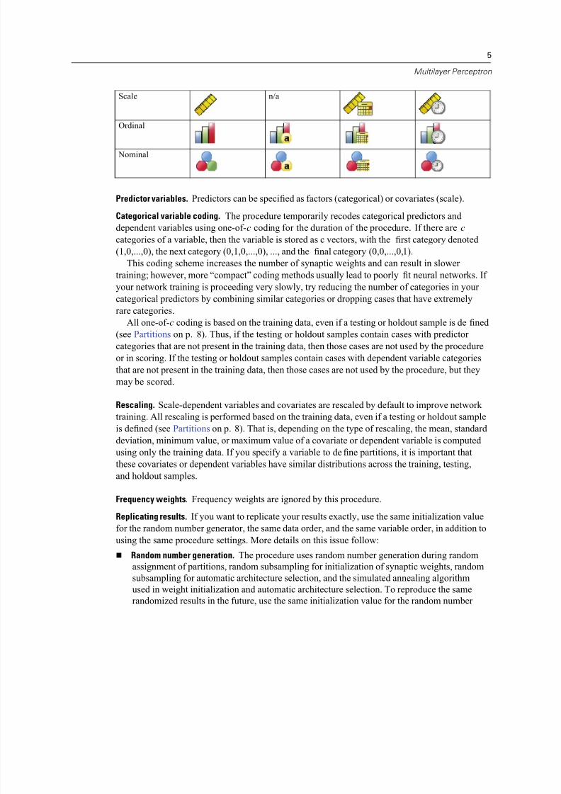
An icon next to each variable in the variable list identifies the measurement level and data type:
Data TypeMeasurementLevel
Numeric String Date Time
4
8/8/2019 SPSS Neural Network 16.0
http://slidepdf.com/reader/full/spss-neural-network-160 15/107
5
Multilayer Perceptron
Scale n/a
Ordinal
Nominal
Predictor variables. Predictors can be specified as factors (categorical) or covariates (scale).
Categorical variable coding. The procedure temporarily recodes categorical predictors and
dependent variables using one-of-c coding for the duration of the procedure. If there are c
categories of a variable, then the variable is stored as c vectors, with the first category denoted
(1,0,...,0), the next category (0,1,0,...,0), ..., and the final category (0,0,...,0,1).
This coding scheme increases the number of synaptic weights and can result in slower
training; however, more “compact” coding methods usually lead to poorlyfi
t neural networks. If your network training is proceeding very slowly, try reducing the number of categories in your
categorical predictors by combining similar categories or dropping cases that have extremely
rare categories.
All one-of-c coding is based on the training data, even if a testing or holdout sample is de fined
(see Partitions on p. 8). Thus, if the testing or holdout samples contain cases with predictor
categories that are not present in the training data, then those cases are not used by the procedure
or in scoring. If the testing or holdout samples contain cases with dependent variable categories
that are not present in the training data, then those cases are not used by the procedure, but they
may be scored.
Rescaling. Scale-dependent variables and covariates are rescaled by default to improve network
training. All rescaling is performed based on the training data, even if a testing or holdout sampleis defined (see Partitions on p. 8). That is, depending on the type of rescaling, the mean, standard
deviation, minimum value, or maximum value of a covariate or dependent variable is computed
using only the training data. If you specify a variable to define partitions, it is important that
these covariates or dependent variables have similar distributions across the training, testing,
and holdout samples.
Frequency weights. Frequency weights are ignored by this procedure.
Replicating results. If you want to replicate your results exactly, use the same initialization value
for the random number generator, the same data order, and the same variable order, in addition to
using the same procedure settings. More details on this issue follow:
Random number generation. The procedure uses random number generation during randomassignment of partitions, random subsampling for initialization of synaptic weights, random
subsampling for automatic architecture selection, and the simulated annealing algorithm
used in weight initialization and automatic architecture selection. To reproduce the same
randomized results in the future, use the same initialization value for the random number

8/8/2019 SPSS Neural Network 16.0
http://slidepdf.com/reader/full/spss-neural-network-160 16/107
6
Chapter 2
generator before each run of the Multilayer Perceptron procedure. See Preparing the Data for
Analysis on p. 35 for step-by-step instructions.
Case order. The Online and Mini-batch training methods (see Training on p. 12) are explicitly
dependent upon case order; however, even Batch training is dependent upon case order because initialization of synaptic weights involves subsampling from the dataset.
To minimize order effects, randomly order the cases. To verify the stability of a given solution,
you may want to obtain several different solutions with cases sorted in different random
orders. In situations with extremely large file sizes, multiple runs can be performed with a
sample of cases sorted in different random orders.
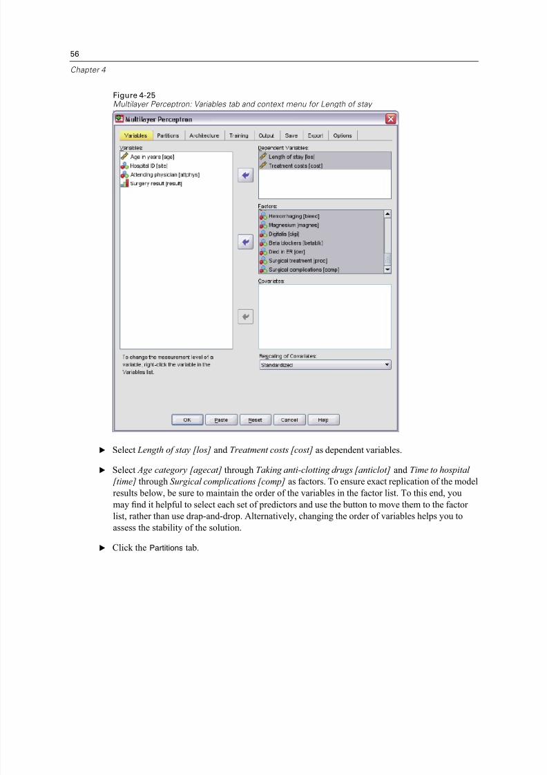
Variable order. Results may be influenced by the order of variables in the factor and covariate
lists due to the different pattern of initial values assigned when the variable order is changed.
As with case order effects, you might try different variable orders (simply drag and drop
within the factor and covariate lists) to assess the stability of a given solution.
Creating a Multilayer Perceptron Network
From the menus choose:
AnalyzeNeural Networks
Multilayer Perceptron...

8/8/2019 SPSS Neural Network 16.0
http://slidepdf.com/reader/full/spss-neural-network-160 17/107
7
Multilayer Perceptron
Figure 2-1Multilayer Perceptron: Variables tab
E Select at least one dependent variable.
E Select at least one factor or covariate.
Optionally, on the Variables tab you can change the method for rescaling covariates. The choices
are:
Standardized. Subtract the mean and divide by the standard deviation, ( x−mean)/ s.
Normalized. Subtract the minimum and divide by the range, ( x−min)/(max−min). Normalized
values fall between 0 and 1. Adjus ted Normalized. Adjusted version of subtracting the minimum and dividing by the range,
[2*( x−min)/(max−min)]−1. Adjusted normalized values fall between −1 and 1.
None. No rescaling of covariates.
8/8/2019 SPSS Neural Network 16.0
http://slidepdf.com/reader/full/spss-neural-network-160 18/107
8
Chapter 2
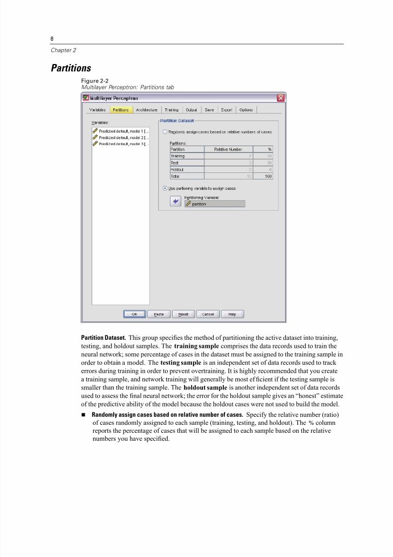
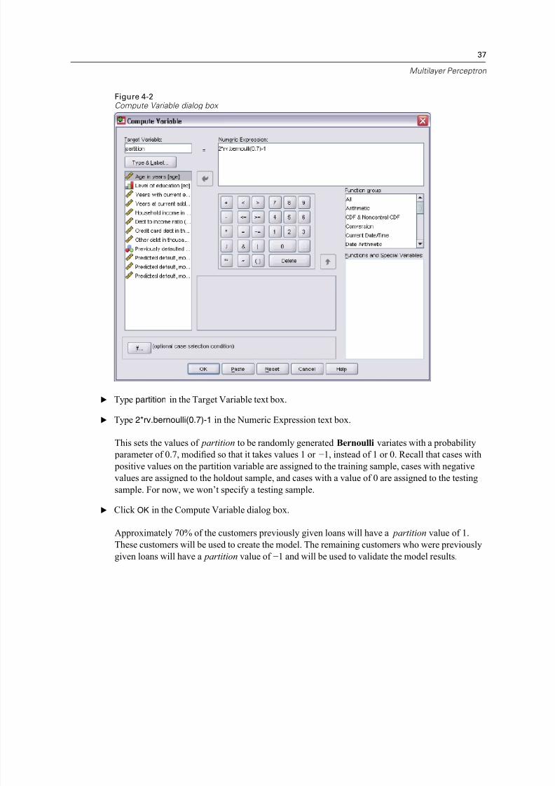
Partitions Figure 2-2Multilayer Perceptron: Partitions tab
Partition Dataset. This group specifies the method of partitioning the active dataset into training,
testing, and holdout samples. The training sample comprises the data records used to train the
neural network; some percentage of cases in the dataset must be assigned to the training sample in
order to obtain a model. The testing sample is an independent set of data records used to track
errors during training in order to prevent overtraining. It is highly recommended that you create
a training sample, and network training will generally be most ef ficient if the testing sample is
smaller than the training sample. The holdout sample is another independent set of data recordsused to assess the final neural network; the error for the holdout sample gives an “honest” estimate
of the predictive ability of the model because the holdout cases were not used to build the model.
Randomly assign cases based on relative number of cases. Specify the relative number (ratio)
of cases randomly assigned to each sample (training, testing, and holdout). The % column
reports the percentage of cases that will be assigned to each sample based on the relative
numbers you have specified.

8/8/2019 SPSS Neural Network 16.0
http://slidepdf.com/reader/full/spss-neural-network-160 19/107
9
Multilayer Perceptron
For example, specifying 7, 3, 0 as the relative numbers for training, testing, and holdout
samples corresponds to 70%, 30%, and 0%. Specifying 2, 1, 1 as the relative numbers
corresponds to 50%, 25%, and 25%; 1, 1, 1 corresponds to dividing the dataset into equal
thirds among training, testing, and holdout.
Use partitioning variable to assign cases. Specify a numeric variable that assigns each case
in the active dataset to the training, testing, or holdout sample. Cases with a positive value
on the variable are assigned to the training sample, cases with a value of 0, to the testing
sample, and cases with a negative value, to the holdout sample. Cases with a system-missing
value are excluded from the analysis. Any user-missing values for the partition variable
are always treated as valid.
Note: Using a partitioning variable will not guarantee identical results in successive runs of
the procedure. See “Replicating results” in the main Multilayer Perceptron topic.
Architecture Figure 2-3Multilayer Perceptron: Architecture tab
8/8/2019 SPSS Neural Network 16.0
http://slidepdf.com/reader/full/spss-neural-network-160 20/107
8/8/2019 SPSS Neural Network 16.0
http://slidepdf.com/reader/full/spss-neural-network-160 21/107
11
Multilayer Perceptron
Hyperbolic tangent. This function has the form: γ(c) = tanh(c) = (ec−e−c)/(ec+e−c). It takes
real-valued arguments and transforms them to the range (–1, 1).
Sigmoid. This function has the form: γ(c) = 1/(1+e−c). It takes real-valued arguments and
transforms them to the range (0, 1).
Rescaling of Scale Dependent Variables. These controls are available only if at least one
scale-dependent variable has been selected.
Standardized. Subtract the mean and divide by the standard deviation, ( x−mean)/ s.
Normalized. Subtract the minimum and divide by the range, ( x−min)/(max−min). Normalized
values fall between 0 and 1. This is the required rescaling method for scale-dependent
variables if the output layer uses the sigmoid activation function. The correction option
specifies a small number ε that is applied as a correction to the rescaling formula;
this correction ensures that all rescaled dependent variable values will be within the
range of the activation function. In particular, the values 0 and 1, which occur in the
uncorrected formula when x takes its minimum and maximum value, define the limits of
the range of the sigmoid function but are not within that range. The corrected formula is[ x−(min−ε)]/[(max+ε)−(min−ε)]. Specify a number greater than or equal to 0.
Adjusted Normalized. Adjusted version of subtracting the minimum and dividing by the range,
[2*( x−min)/(max−min)]−1. Adjusted normalized values fall between −1 and 1. This is the
required rescaling method for scale-dependent variables if the output layer uses the hyperbolic
tangent activation function. The correction option specifies a small number ε that is applied
as a correction to the rescaling formula; this correction ensures that all rescaled dependent
variable values will be within the range of the activation function. In particular, the values−1 and 1, which occur in the uncorrected formula when x takes its minimum and maximum
value, define the limits of the range of the hyperbolic tangent function but are not within that
range. The corrected formula is {2*[( x−(min−ε))/((max+ε)−(min−ε))]}−1. Specify a number
greater than or equal to 0.
None. No rescaling of scale-dependent variables.
8/8/2019 SPSS Neural Network 16.0
http://slidepdf.com/reader/full/spss-neural-network-160 22/107
12
Chapter 2
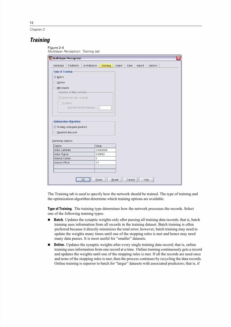
Training Figure 2-4Multilayer Perceptron: Training tab
The Training tab is used to specify how the network should be trained. The type of training and
the optimization algorithm determine which training options are available.
Type of Training. The training type determines how the network processes the records. Select
one of the following training types:
Batch. Updates the synaptic weights only after passing all training data records; that is, batch
training uses information from all records in the training dataset. Batch training is often
preferred because it directly minimizes the total error; however, batch training may need toupdate the weights many times until one of the stopping rules is met and hence may need
many data passes. It is most useful for “smaller” datasets.
Online. Updates the synaptic weights after every single training data record; that is, online
training uses information from one record at a time. Online training continuously gets a record
and updates the weights until one of the stopping rules is met. If all the records are used once
and none of the stopping rules is met, then the process continues by recycling the data records.
Online training is superior to batch for “larger” datasets with associated predictors; that is, if
8/8/2019 SPSS Neural Network 16.0
http://slidepdf.com/reader/full/spss-neural-network-160 23/107
13
Multilayer Perceptron
there are many records and many inputs, and their values are not independent of each other,
then online training can more quickly obtain a reasonable answer than batch training.
Mini-batch. Divides the training data records into groups of approximately equal size, then
updates the synaptic weights after passing one group; that is, mini-batch training usesinformation from a group of records. Then the process recycles the data group if necessary.
Mini-batch training offers a compromise between batch and online training, and it may be
best for “medium-size” datasets. The procedure can automatically determine the number of
training records per mini-batch, or you can specify an integer greater than 1 and less than or
equal to the maximum number of cases to store in memory. You can set the maximum number
of cases to store in memory on the Options tab.
Optimization Algorithm. This is the method used to estimate the synaptic weights.
Scaled conjugate gradient. The assumptions that justify the use of conjugate gradient methods
apply only to batch training types, so this method is not available for online or mini-batch
training.
Gradient descent. This method must be used with online or mini-batch training; it can also beused with batch training.
Training Options. The training options allow you to fine-tune the optimization algorithm. You
generally will not need to change these settings unless the network runs into problems with
estimation.
Training options for the scaled conjugate gradient algorithm include:
Initial Lambda. The initial value of the lambda parameter for the scaled conjugate gradient
algorithm. Specify a number greater than 0 and less than 0.000001.
Initial Sigma. The initial value of the sigma parameter for the scaled conjugate gradient
algorithm. Specify a number greater than 0 and less than 0.0001. Interval Center and Interval Offset. The interval center (a0) and interval offset (a) define the
interval [a0−a, a0+a], in which weight vectors are randomly generated when simulated
annealing is used. Simulated annealing is used to break out of a local minimum, with the
goal of finding the global minimum, during application of the optimization algorithm. This
approach is used in weight initialization and automatic architecture selection. Specify a
number for the interval center and a number greater than 0 for the interval offset.
Training options for the gradient descent algorithm include:
Initial Learning Rate. The initial value of the learning rate for the gradient descent algorithm. A
higher learning rate means that the network will train faster, possibly at the cost of becoming
unstable. Specify a number greater than 0.
Lower Boundary of Learning Rate. The lower boundary on the learning rate for the gradient
descent algorithm. This setting applies only to online and mini-batch training. Specify a
number greater than 0 and less than the initial learning rate.
8/8/2019 SPSS Neural Network 16.0
http://slidepdf.com/reader/full/spss-neural-network-160 24/107
14
Chapter 2
Momentum. The initial momentum parameter for the gradient descent algorithm. The
momentum term helps to prevent instabilities caused by a too-high learning rate. Specify
a number greater than 0.
Learning rate reduction, in Epochs. The number of epochs ( p), or data passes of the trainingsample, required to reduce the initial learning rate to the lower boundary of the learning rate
when gradient descent is used with online or mini-batch training. This gives you control of the
learning rate decay factor β = (1/ pK )*ln(η0/ηlow), where η0 is the initial learning rate, ηlow is
the lower bound on the learning rate, and K is the total number of mini-batches (or the number
of training records for online training) in the training dataset. Specify an integer greater than 0.
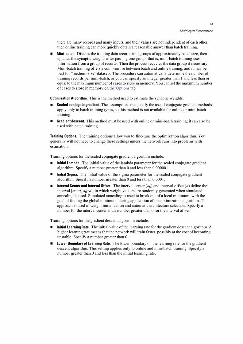
Output Figure 2-5Multilayer Perceptron: Output tab
Network Structure. Displays summary information about the neural network.
Description. Displays information about the neural network, including the dependent variables,
number of input and output units, number of hidden layers and units, and activation functions.

8/8/2019 SPSS Neural Network 16.0
http://slidepdf.com/reader/full/spss-neural-network-160 25/107
15
Multilayer Perceptron
Diagram. Displays the network diagram as a non-editable chart. Note that as the number of
covariates and factor levels increases, the diagram becomes more dif ficult to interpret.
Synaptic weights. Displays the coef ficient estimates that show the relationship between the
units in a given layer to the units in the following layer. The synaptic weights are based on thetraining sample even if the active dataset is partitioned into training, testing, and holdout data.
Note that the number of synaptic weights can become rather large and that these weights are
generally not used for interpreting network results.
Network Performance. Displays results used to determine whether the model is “good”. Note:
Charts in this group are based on the combined training and testing samples or only on the training
sample if there is no testing sample.
Model summary. Displays a summary of the neural network results by partition and overall,
including the error, the relative error or percentage of incorrect predictions, the stopping rule
used to stop training, and the training time.
The error is the sum-of-squares error when the identity, sigmoid, or hyperbolic tangent
activation function is applied to the output layer. It is the cross-entropy error when the softmaxactivation function is applied to the output layer.
Relative errors or percentages of incorrect predictions are displayed depending on the
dependent variable measurement levels. If any dependent variable has scale measurement
level, then the average overall relative error (relative to the mean model) is displayed. If all
dependent variables are categorical, then the average percentage of incorrect predictions
is displayed. Relative errors or percentages of incorrect predictions are also displayed for
individual dependent variables.
Classification results. Displays a classification table for each categorical dependent variable by
partition and overall. Each table gives the number of cases classified correctly and incorrectly
for each dependent variable category. The percentage of the total cases that were correctly
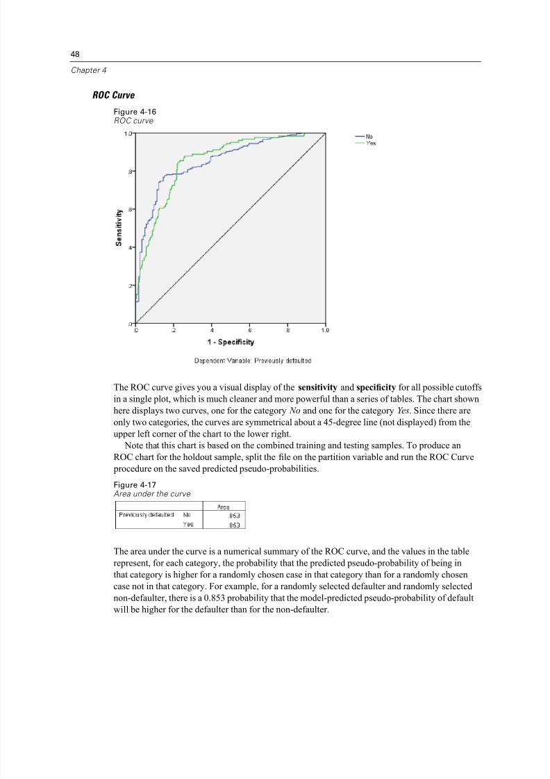
classified is also reported. ROC curve. Displays an ROC (Receiver Operating Characteristic) curve for each categorical
dependent variable. It also displays a table giving the area under each curve. For a given
dependent variable, the ROC chart displays one curve for each category. If the dependent
variable has two categories, then each curve treats the category at issue as the positive state
versus the other category. If the dependent variable has more than two categories, then
each curve treats the category at issue as the positive state versus the aggregate of all other
categories.
Cumulative gains chart. Displays a cumulative gains chart for each categorical dependent
variable. The display of one curve for each dependent variable category is the same as for
ROC curves.
Lift chart. Displays a lift chart for each categorical dependent variable. The display of onecurve for each dependent variable category is the same as for ROC curves.

8/8/2019 SPSS Neural Network 16.0
http://slidepdf.com/reader/full/spss-neural-network-160 26/107
16
Chapter 2
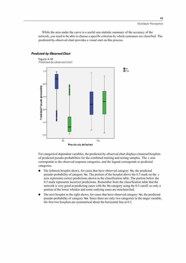
Predicted by observed chart. Displays a predicted-by-observed-value chart for each
dependent variable. For categorical dependent variables, clustered boxplots of predicted
pseudo-probabilities are displayed for each response category, with the observed response
category as the cluster variable. For scale-dependent variables, a scatterplot is displayed.
Residual by predicted chart. Displays a residual-by-predicted-value chart for each
scale-dependent variable. There should be no visible patterns between residuals and predicted
values. This chart is produced only for scale-dependent variables.
Case processing summary. Displays the case processing summary table, which summarizes the
number of cases included and excluded in the analysis, in total and by training, testing, and
holdout samples.
Independent variable importance analysis. Performs a sensitivity analysis, which computes the
importance of each predictor in determining the neural network. The analysis is based on
the combined training and testing samples or only on the training sample if there is no testing
sample. This creates a table and a chart displaying importance and normalized importance for each predictor. Note that sensitivity analysis is computationally expensive and time-consuming if
there are large numbers of predictors or cases.

8/8/2019 SPSS Neural Network 16.0
http://slidepdf.com/reader/full/spss-neural-network-160 27/107
17
Multilayer Perceptron
Save Figure 2-6Multilayer Perceptron: Save tab
The Save tab is used to save predictions as variables in the dataset.
Save predicted value or category for each dependent variable. This saves the predicted value for
scale-dependent variables and the predicted category for categorical dependent variables.
Save predicted pseudo-probability or category for each dependent variable. This saves the
predicted pseudo-probabilities for categorical dependent variables. A separate variable is
saved for each of the first n categories, where n is specified in the Categories to Save column.
Names of Saved Variables. Automatic name generation ensures that you keep all of your work.Custom names allow you to discard/replace results from previous runs without first deleting the
saved variables in the Data Editor.

8/8/2019 SPSS Neural Network 16.0
http://slidepdf.com/reader/full/spss-neural-network-160 28/107
18
Chapter 2
Probabilities and Pseudo-Probabilities
Categorical dependent variables with softmax activation and cross-entropy error will have a
predicted value for each category, where each predicted value is the probability that the case
belongs to the category.
Categorical dependent variables with sum-of-squares error will have a predicted value for each
category, but the predicted values cannot be interpreted as probabilities. The procedure saves
these predicted pseudo-probabilities even if any are less than 0 or greater than 1, or the sum for a
given dependent variable is not 1.
The ROC, cumulative gains, and lift charts (see Output on p. 14) are created based on
pseudo-probabilities. In the event that any of the pseudo-probabilities are less than 0 or greater
than 1, or the sum for a given variable is not 1, they are first rescaled to be between 0 and 1 and to
sum to 1. Pseudo-probabilities are rescaled by dividing by their sum. For example, if a case has
predicted pseudo-probabilities of 0.50, 0.60, and 0.40 for a three-category dependent variable,
then each pseudo-probability is divided by the sum 1.50 to get 0.33, 0.40, and 0.27.
If any of the pseudo-probabilities are negative, then the absolute value of the lowest is added toall pseudo-probabilities before the above rescaling. For example, if the pseudo-probabilities are
-0.30, 0.50, and 1.30, then first add 0.30 to each value to get 0.00, 0.80, and 1.60. Next, divide
each new value by the sum 2.40 to get 0.00, 0.33, and 0.67.

8/8/2019 SPSS Neural Network 16.0
http://slidepdf.com/reader/full/spss-neural-network-160 29/107
19
Multilayer Perceptron
Export Figure 2-7Multilayer Perceptron: Export tab
The Export tab is used to save the synaptic weight estimates for each dependent variable to an
XML (PMML) file. SmartScore and SPSS Server (a separate product) can use this model file to
apply the model information to other data files for scoring purposes. This option is not available if
split files have been defined.
8/8/2019 SPSS Neural Network 16.0
http://slidepdf.com/reader/full/spss-neural-network-160 30/107
20
Chapter 2
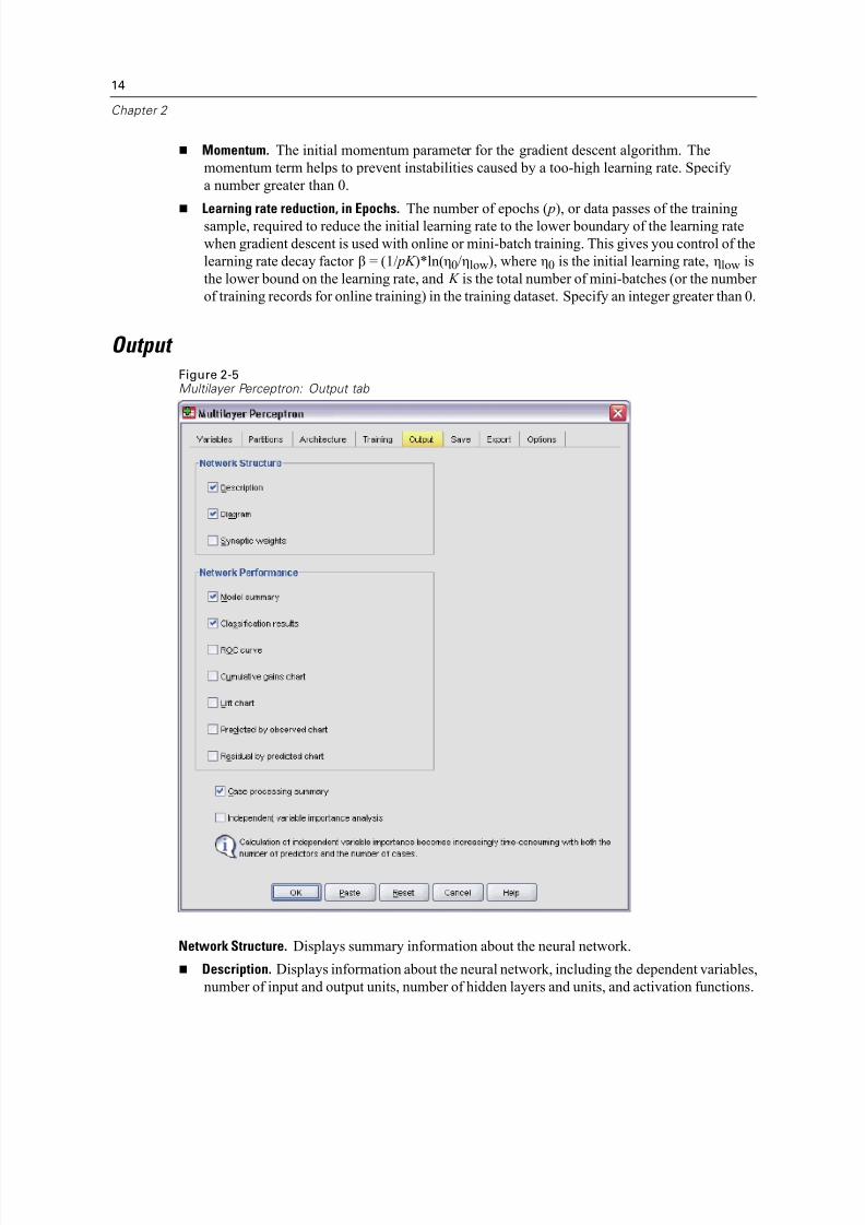
Options Figure 2-8Multilayer Perceptron: Options tab
User-Missing Values. Factors must have valid values for a case to be included in the analysis.
These controls allow you to decide whether user-missing values are treated as valid among factors
and categorical dependent variables.
Stopping Rules. These are the rules that determine when to stop training the neural network.
Training proceeds through at least one data pass. Training can then be stopped according to the
following criteria, which are checked in the listed order. In the stopping rule definitions thatfollow, a step corresponds to a data pass for the online and mini-batch methods and an iteration
for the batch method.
Maximum steps without a decrease in error. The number of steps to allow before checking for
a decrease in error. If there is no decrease in error after the specified number of steps, then
training stops. Specify an integer greater than 0. You can also specify which data sample is
used to compute the error. Choose automatically uses the testing sample if it exists and uses
the training sample otherwise. Note that batch training guarantees a decrease in the training

8/8/2019 SPSS Neural Network 16.0
http://slidepdf.com/reader/full/spss-neural-network-160 31/107
21
Multilayer Perceptron
sample error after each data pass; thus, this option applies only to batch training if a testing
sample exists. Both training and test data checks the error for each of these samples; this
option applies only if a testing sample exits.
Note: After each complete data pass, online and mini-batch training require an extra data passin order to compute the training error. This extra data pass can slow training considerably, so
it is generally recommended that you supply a testing sample and select Choose automatically
in any case.
Maximum training time. Choose whether to specify a maximum number of minutes for the
algorithm to run. Specify a number greater than 0.
Maximum Training Epochs. The maximum number of epochs (data passes) allowed. If the
maximum number of epochs is exceeded, then training stops. Specify an integer greater than 0.
Minimum relative change in training error. Training stops if the relative change in the training
error compared to the previous step is less than the criterion value. Specify a number greater
than 0. For online and mini-batch training, this criterion is ignored if only testing data is
used to compute the error.
Minimum relative change in training error ratio. Training stops if the ratio of the training error to
the error of the null model is less than the criterion value. The null model predicts the average
value for all dependent variables. Specify a number greater than 0. For online and mini-batch
training, this criterion is ignored if only testing data is used to compute the error.
Maximum cases to store in memory. This controls the following settings within the multilayer
perceptron algorithms. Specify an integer greater than 1.
In automatic architecture selection, the size of the sample used to determine the network
archicteture is min(1000,memsize), where memsize is the maximum number of cases to store
in memory.
In mini-batch training with automatic computation of the number of mini-batches, the
number of mini-batches is min(max(M /10,2),memsize), where M is the number of cases in
the training sample.
8/8/2019 SPSS Neural Network 16.0
http://slidepdf.com/reader/full/spss-neural-network-160 32/107
Chapter
3Radial Basis Function
The Radial Basis Function (RBF) procedure produces a predictive model for one or more
dependent (target) variables based on values of predictor variables.
Example. A telecommunications provider has segmented its customer base by service usage
patterns, categorizing the customers into four groups. An RBF network using demographic data
to predict group membership allows the company to customize offers for individual prospective
customers.
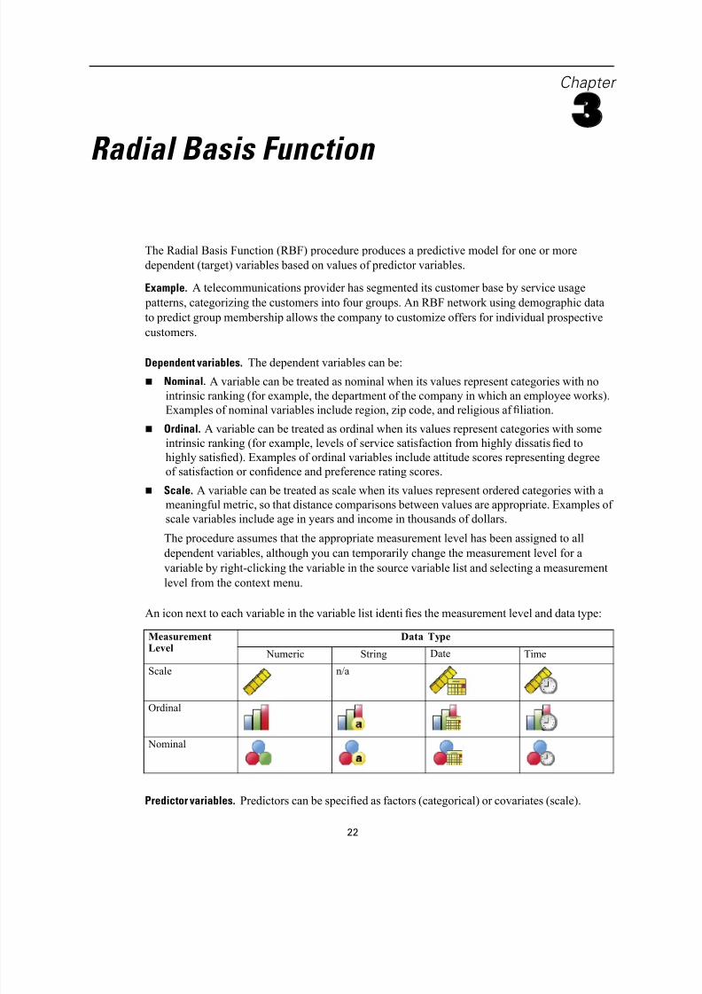
Dependent variables. The dependent variables can be:
Nominal. A variable can be treated as nominal when its values represent categories with no
intrinsic ranking (for example, the department of the company in which an employee works).
Examples of nominal variables include region, zip code, and religious af filiation.
Ordinal. A variable can be treated as ordinal when its values represent categories with some
intrinsic ranking (for example, levels of service satisfaction from highly dissatisfied to
highly satisfied). Examples of ordinal variables include attitude scores representing degree
of satisfaction or confidence and preference rating scores.
Scale. A variable can be treated as scale when its values represent ordered categories with a
meaningful metric, so that distance comparisons between values are appropriate. Examples of
scale variables include age in years and income in thousands of dollars.The procedure assumes that the appropriate measurement level has been assigned to all
dependent variables, although you can temporarily change the measurement level for a
variable by right-clicking the variable in the source variable list and selecting a measurement
level from the context menu.
An icon next to each variable in the variable list identifies the measurement level and data type:
Data TypeMeasurementLevel
Numeric String Date Time
Scale n/a
Ordinal
Nominal
Predictor variables. Predictors can be specified as factors (categorical) or covariates (scale).
22
8/8/2019 SPSS Neural Network 16.0
http://slidepdf.com/reader/full/spss-neural-network-160 33/107
23
Radial Basis Function
Categorical variable coding. The procedure temporarily recodes categorical predictors and
dependent variables using one-of-c coding for the duration of the procedure. If there are c
categories of a variable, then the variable is stored as c vectors, with the first category denoted
(1,0,...,0), the next category (0,1,0,...,0), ..., and the final category (0,0,...,0,1).
This coding scheme increases the number of synaptic weights and can result in slower training,
but more “compact” coding methods usually lead to poorly fit neural networks. If your network
training is proceeding very slowly, try reducing the number of categories in your categorical
predictors by combining similar categories or dropping cases that have extremely rare categories.
All one-of-c coding is based on the training data, even if a testing or holdout sample is de fined
(see Partitions on p. 25). Thus, if the testing or holdout samples contain cases with predictor
categories that are not present in the training data, then those cases are not used by the procedure
or in scoring. If the testing or holdout samples contain cases with dependent variable categories
that are not present in the training data, then those cases are not used by the procedure but they
may be scored.
Rescaling. Scale dependent variables and covariates are rescaled by default to improve network training. All rescaling is performed based on the training data, even if a testing or holdout sample
is defined (see Partitions on p. 25). That is, depending on the type of rescaling, the mean, standard
deviation, minimum value, or maximum value of a covariate or dependent variable are computed
using only the training data. If you specify a variable to define partitions, it is important that
these covariates or dependent variables have similar distributions across the training, testing,
and holdout samples.
Frequency weights. Frequency weights are ignored by this procedure.
Replicating results. If you want to exactly replicate your results, use the same initialization value
for the random number generator and the same data order, in addition to using the same proceduresettings. More details on this issue follow:
Random number generation. The procedure uses random number generation during random
assignment of partitions. To reproduce the same randomized results in the future, use the
same initialization value for the random number generator before each run of the Radial Basis
Function procedure. See Preparing the Data for Analysis on p. 71 for step-by-step instructions.
Case order. Results are also dependent on data order because the two-step cluster algorithm is
used to determine the radial basis functions.
To minimize order effects, randomly order the cases. To verify the stability of a given solution,
you may want to obtain several different solutions with cases sorted in different random
orders. In situations with extremely large file sizes, multiple runs can be performed with a
sample of cases sorted in different random orders.
Creating a Radial Basis Function Network
From the menus choose:
AnalyzeNeural Networks
Radial Basis Function...
8/8/2019 SPSS Neural Network 16.0
http://slidepdf.com/reader/full/spss-neural-network-160 34/107
24
Chapter 3
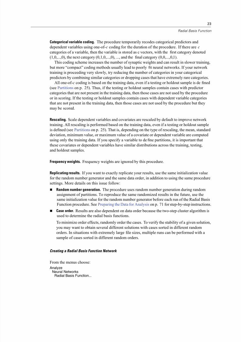
Figure 3-1Radial Basis Function: Variables tab
E Select at least one dependent variable.
E Select at least one factor or covariate.
Optionally, on the Variables tab you can change the method for rescaling covariates. The choices
are:
Standardized. Subtract the mean and divide by the standard deviation, ( x−mean)/ s.
Normalized. Subtract the minimum and divide by the range, ( x−min)/(max−min). Normalized
values fall between 0 and 1.
Adjusted Normalized. Adjusted version of subtracting the minimum and dividing by the range,
[2*( x−min)/(max−min)]−1. Adjusted normalized values fall between −1 and 1.
None. No rescaling of covariates.

8/8/2019 SPSS Neural Network 16.0
http://slidepdf.com/reader/full/spss-neural-network-160 35/107
25
Radial Basis Function
Partitions Figure 3-2Radial Basis Function: Partitions tab
Partition Dataset. This group specifies the method of partitioning the active dataset into training,
testing, and holdout samples. The training sample comprises the data records used to train the
neural network; some percentage of cases in the dataset must be assigned to the training sample in
order to obtain a model. The testing sample is an independent set of data records used to track
errors during training in order to prevent overtraining. It is highly recommended that you create
a training sample, and network training will generally be most ef ficient if the testing sample is
smaller than the training sample. The holdout sample is another independent set of data records
used to assess the final neural network; the error for the holdout sample gives an “honest” estimate
of the predictive ability of the model because the holdout cases were not used to build the model.
Randomly assign cases based on relative number of cases. Specify the relative number (ratio)
of cases randomly assigned to each sample (training, testing, and holdout). The % column
reports the percentage of cases that will be assigned to each sample based on the relative
numbers you have specified.
8/8/2019 SPSS Neural Network 16.0
http://slidepdf.com/reader/full/spss-neural-network-160 36/107
26
Chapter 3
For example, specifying 7, 3, 0 as the relative numbers for training, testing, and holdout
samples corresponds to 70%, 30%, and 0%. Specifying 2, 1, 1 as the relative numbers
corresponds to 50%, 25%, and 25%; 1, 1, 1 corresponds to dividing the dataset into equal
thirds among training, testing, and holdout.
Use partitioning variable to assign cases. Specify a numeric variable that assigns each case
in the active dataset to the training, testing, or holdout sample. Cases with a positive value
on the variable are assigned to the training sample, cases with a value of 0, to the testing
sample, and cases with a negative value, to the holdout sample. Cases with a system-missing
value are excluded from the analysis. Any user-missing values for the partition variable
are always treated as valid.
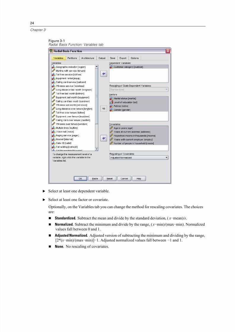
Architecture Figure 3-3Radial Basis Function: Architecture tab
The Architecture tab is used to specify the structure of the network. The procedure creates a
neural network with one hidden “radial basis function” layer; in general, it will not be necessary to
change these settings.

8/8/2019 SPSS Neural Network 16.0
http://slidepdf.com/reader/full/spss-neural-network-160 37/107
27
Radial Basis Function
Number of Units in Hidden Layer. There are three ways of choosing the number of hidden units.
1. Find the best number of units within an automatically computed range. The procedure automatically
computes the minimum and maximum values of the range and finds the best number of hidden
units within the range.
If a testing sample is defined, then the procedure uses the testing data criterion: The best number
of hidden units is the one that yields the smallest error in the testing data. If a testing sample is not
defined, then the procedure uses the Bayesian information criterion (BIC): The best number of
hidden units is the one that yields the smallest BIC based on the training data.
2. Find the best number of units within a specified range. You can provide your own range, and the
procedure will find the “best” number of hidden units within that range. As before, the best
number of hidden units from the range is determined using the testing data criterion or the BIC.
3. Use a specified number of units. You can override the use of a range and specify a particular
number of units directly.
Activation Function for Hidden Layer. The activation function for the hidden layer is the radial basis
function, which “links” the units in a layer to the values of units in the succeeding layer. For the
output layer, the activation function is the identity function; thus, the output units are simply
weighted sums of the hidden units.
Normalized radial basis function. Uses the softmax activation function so the activations of
all hidden units are normalized to sum to 1.
Ordinary radial basis function. Uses the exponential activation function so the activation of the
hidden unit is a Gaussian “bump” as a function of the inputs.
Overlap Among Hidden Units. The overlapping factor is a multiplier applied to the width of the
radial basis functions. The automatically computed value of the overlapping factor is 1+0.1d ,
where d is the number of input units (the sum of the number of categories across all factors and
the number of covariates).
8/8/2019 SPSS Neural Network 16.0
http://slidepdf.com/reader/full/spss-neural-network-160 38/107
28
Chapter 3
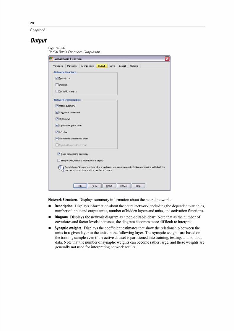
Output Figure 3-4Radial Basis Function: Output tab
Network Structure. Displays summary information about the neural network.
Description. Displays information about the neural network, including the dependent variables,
number of input and output units, number of hidden layers and units, and activation functions.
Diagram. Displays the network diagram as a non-editable chart. Note that as the number of
covariates and factor levels increases, the diagram becomes more dif ficult to interpret.
Synaptic weights. Displays the coef ficient estimates that show the relationship between the
units in a given layer to the units in the following layer. The synaptic weights are based onthe training sample even if the active dataset is partitioned into training, testing, and holdout
data. Note that the number of synaptic weights can become rather large, and these weights are
gener ally not used for interpreting network results.
8/8/2019 SPSS Neural Network 16.0
http://slidepdf.com/reader/full/spss-neural-network-160 39/107
29
Radial Basis Function
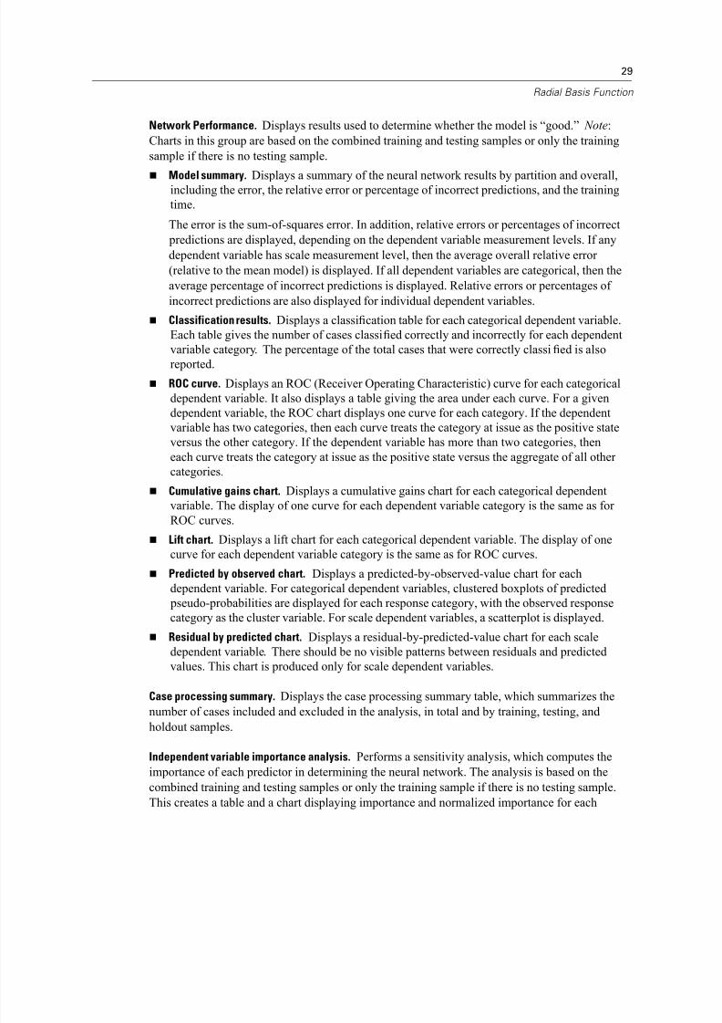
Network Performance. Displays results used to determine whether the model is “good.” Note:
Charts in this group are based on the combined training and testing samples or only the training
sample if there is no testing sample.
Model summary. Displays a summary of the neural network results by partition and overall,including the error, the relative error or percentage of incorrect predictions, and the training
time.
The error is the sum-of-squares error. In addition, relative errors or percentages of incorrect
predictions are displayed, depending on the dependent variable measurement levels. If any
dependent variable has scale measurement level, then the average overall relative error
(relative to the mean model) is displayed. If all dependent variables are categorical, then the
average percentage of incorrect predictions is displayed. Relative errors or percentages of
incorrect predictions are also displayed for individual dependent variables.
Classification results. Displays a classification table for each categorical dependent variable.
Each table gives the number of cases classified correctly and incorrectly for each dependent
variable category. The percentage of the total cases that were correctly classified is also
reported.
ROC curve. Displays an ROC (Receiver Operating Characteristic) curve for each categorical
dependent variable. It also displays a table giving the area under each curve. For a given
dependent variable, the ROC chart displays one curve for each category. If the dependent
variable has two categories, then each curve treats the category at issue as the positive state
versus the other category. If the dependent variable has more than two categories, then
each curve treats the category at issue as the positive state versus the aggregate of all other
categories.
Cumulative gains chart. Displays a cumulative gains chart for each categorical dependent
variable. The display of one curve for each dependent variable category is the same as for
ROC curves.
Lift chart. Displays a lift chart for each categorical dependent variable. The display of onecurve for each dependent variable category is the same as for ROC curves.
Predicted by observed chart. Displays a predicted-by-observed-value chart for each
dependent variable. For categorical dependent variables, clustered boxplots of predicted
pseudo-probabilities are displayed for each response category, with the observed response
category as the cluster variable. For scale dependent variables, a scatterplot is displayed.
Residual by predicted chart. Displays a residual-by-predicted-value chart for each scale
dependent variable. There should be no visible patterns between residuals and predicted
values. This chart is produced only for scale dependent variables.
Case processing summary. Displays the case processing summary table, which summarizes the
number of cases included and excluded in the analysis, in total and by training, testing, andholdout samples.
Independent variable importance analysis. Performs a sensitivity analysis, which computes the
importance of each predictor in determining the neural network. The analysis is based on the
combined training and testing samples or only the training sample if there is no testing sample.
This creates a table and a chart displaying importance and normalized importance for each

8/8/2019 SPSS Neural Network 16.0
http://slidepdf.com/reader/full/spss-neural-network-160 40/107
30
Chapter 3
predictor. Note that sensitivity analysis is computationally expensive and time-consuming if
there is a large number of predictors or cases.
Save
Figure 3-5Radial Basis Function: Save t ab
The Save tab is used to save predictions as variables in the dataset.
Save predicted value or category for each dependent variable. This saves the predicted value for
scale dependent variables and the predicted category for categorical dependent variables.
Save predicted pseudo-probability for each dependent variable. This saves the predicted
pseudo-probabilities for categorical dependent variables. A separate variable is saved for each
of the first n categories, where n is specified in the Categories to Save column.
Names of Saved Variables. Automatic name generation ensures that you keep all of your work.
Custom names allow you to discard or replace results from previous runs without first deleting the
saved variables in the Data Editor.

8/8/2019 SPSS Neural Network 16.0
http://slidepdf.com/reader/full/spss-neural-network-160 41/107
31
Radial Basis Function
Probabilities and Pseudo-Probabilities
Predicted pseudo-probabilities cannot be interpreted as probabilities because the Radial Basis
Function procedure uses the sum-of-squares error and identity activation function for the output
layer. The procedure saves these predicted pseudo-probabilities even if any are less than 0 or
greater than 1 or the sum for a given dependent variable is not 1.
The ROC, cumulative gains, and lift charts (see Output on p. 28) are created based on
pseudo-probabilities. In the event that any of the pseudo-probabilities are less than 0 or greater
than 1 or the sum for a given variable is not 1, they are first rescaled to be between 0 and 1 and to
sum to 1. Pseudo-probabilities are rescaled by dividing by their sum. For example, if a case has
predicted pseudo-probabilities of 0.50, 0.60, and 0.40 for a three-category dependent variable,
then each pseudo-probability is divided by the sum 1.50 to get 0.33, 0.40, and 0.27.
If any of the pseudo-probabilities are negative, then the absolute value of the lowest is added to
all pseudo-probabilities before the above rescaling. For example, if the pseudo-probabilities are
–0.30, .50, and 1.30, then first add 0.30 to each value to get 0.00, 0.80, and 1.60. Next, divide each
new value by the sum 2.40 to get 0.00, 0.33, and 0.67.
8/8/2019 SPSS Neural Network 16.0
http://slidepdf.com/reader/full/spss-neural-network-160 42/107
32
Chapter 3
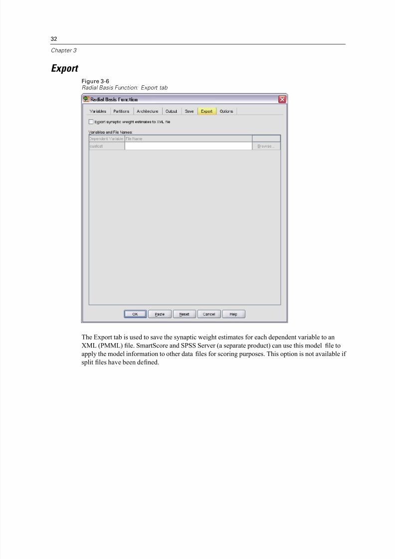
Export Figure 3-6Radial Basis Function: Export tab
The Export tab is used to save the synaptic weight estimates for each dependent variable to an
XML (PMML) file. SmartScore and SPSS Server (a separate product) can use this model file to
apply the model information to other data files for scoring purposes. This option is not available if
split files have been defined.

8/8/2019 SPSS Neural Network 16.0
http://slidepdf.com/reader/full/spss-neural-network-160 43/107

8/8/2019 SPSS Neural Network 16.0
http://slidepdf.com/reader/full/spss-neural-network-160 44/107
8/8/2019 SPSS Neural Network 16.0
http://slidepdf.com/reader/full/spss-neural-network-160 45/107

8/8/2019 SPSS Neural Network 16.0
http://slidepdf.com/reader/full/spss-neural-network-160 46/107
8/8/2019 SPSS Neural Network 16.0
http://slidepdf.com/reader/full/spss-neural-network-160 47/107

8/8/2019 SPSS Neural Network 16.0
http://slidepdf.com/reader/full/spss-neural-network-160 48/107
38
Chapter 4
Running the Analysis
E To run a Multilayer Perceptron analysis, from the menus choose:
Analyze
Neural NetworksMultilayer Perceptron...
Figure 4-3Multilayer Perceptron: Variables tab
E Select Previously defaulted [default] as a dependent variable.
E Select Level of education [ed] as a factor.
E Select Age in years [age] through Other debt in thousands [othdebt] as covariates.
E Click the Partitions tab.
8/8/2019 SPSS Neural Network 16.0
http://slidepdf.com/reader/full/spss-neural-network-160 49/107
39
Multilayer Perceptron
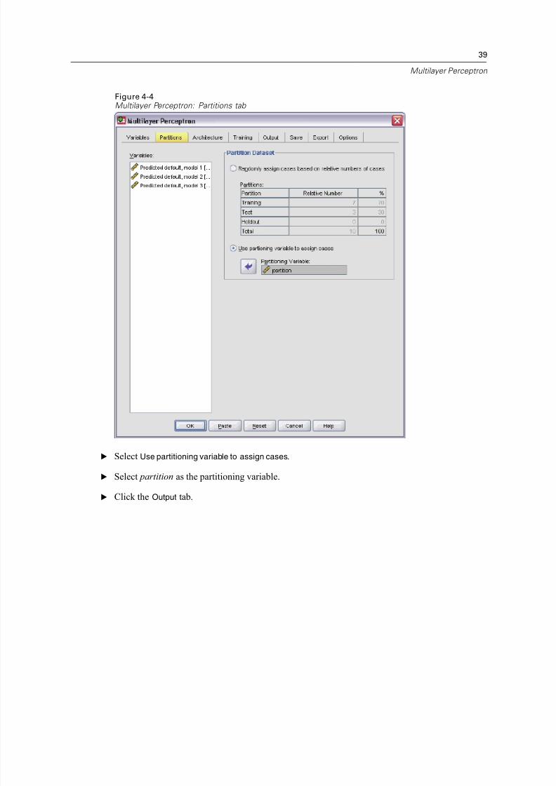
Figure 4-4Multilayer Perceptron: Partitions tab
E Select Use partitioning variable to assign cases.
E Select partition as the partitioning variable.
E Click the Output tab.

8/8/2019 SPSS Neural Network 16.0
http://slidepdf.com/reader/full/spss-neural-network-160 50/107
40
Chapter 4
Figure 4-5Multilayer Perceptron: Output tab
E Deselect Diagram in the Network Structure group.
E Select ROC curve, Cumulative gains chart, Lift chart, and Predicted by observed chart in the Network
Perfor mance group. The Residual by predicted chart is unavailable because the dependent
variable is not scale.
E Select Independent variable importance analysis.
E Click OK.
8/8/2019 SPSS Neural Network 16.0
http://slidepdf.com/reader/full/spss-neural-network-160 51/107

8/8/2019 SPSS Neural Network 16.0
http://slidepdf.com/reader/full/spss-neural-network-160 52/107

8/8/2019 SPSS Neural Network 16.0
http://slidepdf.com/reader/full/spss-neural-network-160 53/107

8/8/2019 SPSS Neural Network 16.0
http://slidepdf.com/reader/full/spss-neural-network-160 54/107

8/8/2019 SPSS Neural Network 16.0
http://slidepdf.com/reader/full/spss-neural-network-160 55/107
8/8/2019 SPSS Neural Network 16.0
http://slidepdf.com/reader/full/spss-neural-network-160 56/107
8/8/2019 SPSS Neural Network 16.0
http://slidepdf.com/reader/full/spss-neural-network-160 57/107
47
Multilayer Perceptron
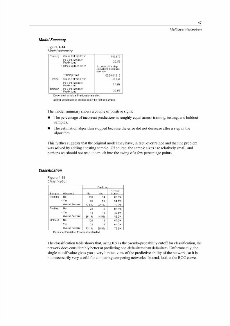
Model Summary
Figure 4-14Model summary
The model summary shows a couple of positive signs:
The percentage of incorrect predictions is roughly equal across training, testing, and holdout
samples.
The estimation algorithm stopped because the error did not decrease after a step in the
algorithm.
This further suggests that the original model may have, in fact, overtrained and that the problem
was solved by adding a testing sample. Of course, the sample sizes are relatively small, and
perhaps we should not read too much into the swing of a few percentage points.
Classification Figure 4-15Classification
The classification table shows that, using 0.5 as the pseudo-probability cutoff for classification, the
network does considerably better at predicting non-defaulters than defaulters. Unfortunately, the
single cutoff value gives you a very limited view of the predictive ability of the network, so it is
not necessarily very useful for comparing competing networks. Instead, look at the ROC curve.
8/8/2019 SPSS Neural Network 16.0
http://slidepdf.com/reader/full/spss-neural-network-160 58/107
8/8/2019 SPSS Neural Network 16.0
http://slidepdf.com/reader/full/spss-neural-network-160 59/107
8/8/2019 SPSS Neural Network 16.0
http://slidepdf.com/reader/full/spss-neural-network-160 60/107
50
Chapter 4
The third boxplot shows, for cases that have observed category Yes, the predicted
pseudo-probability of category No. It and the last boxplot are symmetrical about the
horizontal line at 0.5.
The last boxplot shows, for cases that have observed category Yes, the predicted pseudo-probability of category Yes. The portion of the boxplot above the 0.5 mark on the y
axis represents correct predictions shown in the classification table. The portion below the
0.5 mark represents incorrect predictions. Remember from the classification table that the
network predicts slightly more than half of the cases with the Yes category using the 0.5
cutoff, so a good portion of the box is misclassified.
Looking at the plot, it appears that by lowering the cutoff for classifying a case as Yes from 0.5
to approximately 0.3—this is roughly the value where the top of the second box and the bottom
of the fourth box are—you can increase the chance of correctly catching prospective defaulters
without losing many potential good customers. That is, moving from 0.5 to 0.3 along the second
box incorrectly reclassifies relatively few non-defaulting customers along the whisker as predicted
defaulters, while along the fourth box, this move correctly reclassifi
es many defaulting customerswithin the box as predicted defaulters.
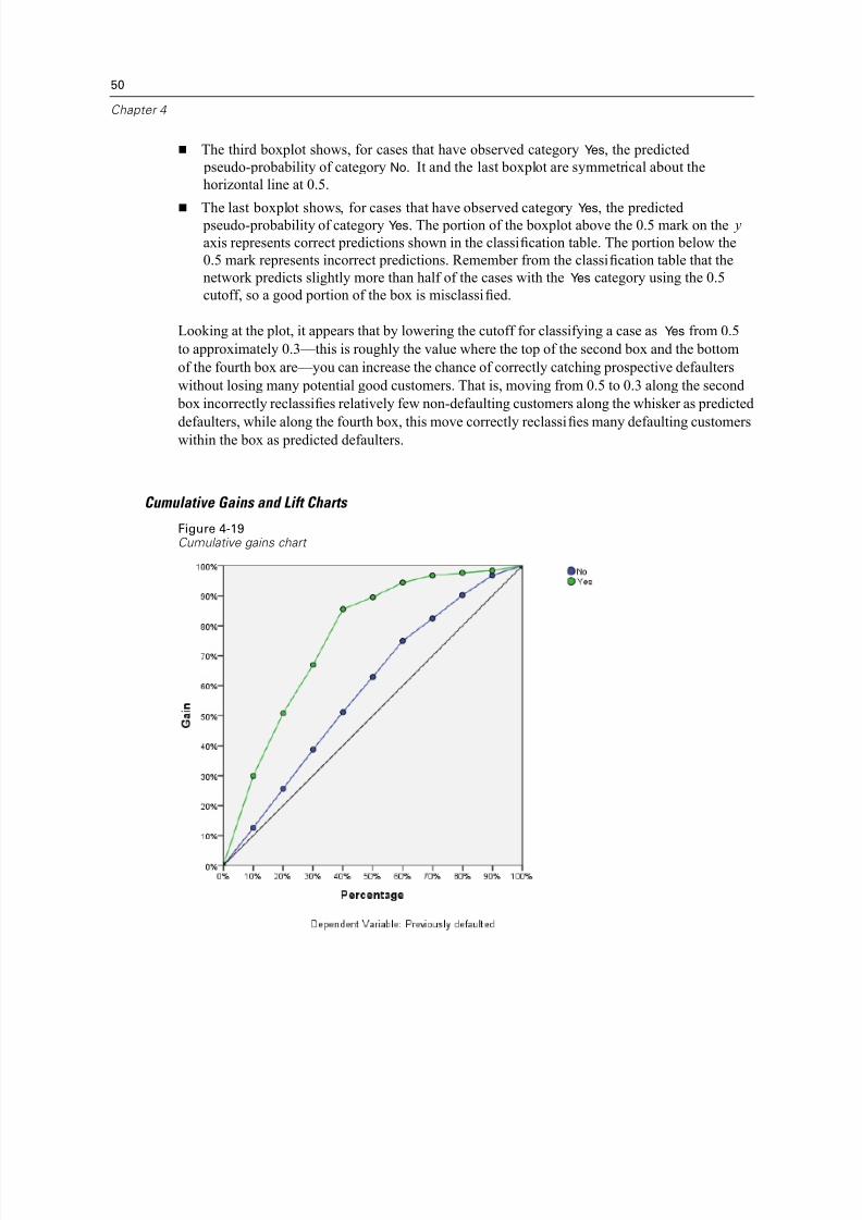
Cumulative Gains and Lift Charts
Figure 4-19Cumulative gains chart

8/8/2019 SPSS Neural Network 16.0
http://slidepdf.com/reader/full/spss-neural-network-160 61/107

8/8/2019 SPSS Neural Network 16.0
http://slidepdf.com/reader/full/spss-neural-network-160 62/107
52
Chapter 4
Figure 4-20Lift chart
The lift chart is derived from the cumulative gains chart; the values on the y axis correspond
to the ratio of the cumulative gain for each curve to the baseline. Thus, the lift at 10% for the
category Yes is 30%/10% = 3.0. It provides another way of looking at the information in the
cumulative gains chart.
Note: The cumulative gains and lift charts are based on the combined training and testing samples.
Independent Variable Importance
Figure 4-21Independent variable importance

8/8/2019 SPSS Neural Network 16.0
http://slidepdf.com/reader/full/spss-neural-network-160 63/107
8/8/2019 SPSS Neural Network 16.0
http://slidepdf.com/reader/full/spss-neural-network-160 64/107
54
Chapter 4
Using a Multilayer Perceptron to Estimate Healthcare Costs and Lengths of Stay
A hospital system is interested in tracking costs and lengths of stay for patients admitted for treatment of myocardial infarction (MI, or “hear t attack”). Obtaining accurate estimates of
these measures allow the administration to properly manage the available bed space as patients
are treated.
The data file patient_los.sav contains the treatment records of a sample of patients who
received treatment for MI. For more information, see Sample Files in Appendix A on p. 84. Use
the Multilayer Perceptron procedure to build a network for predicting costs and length of stay.
Preparing the Data for Analysis
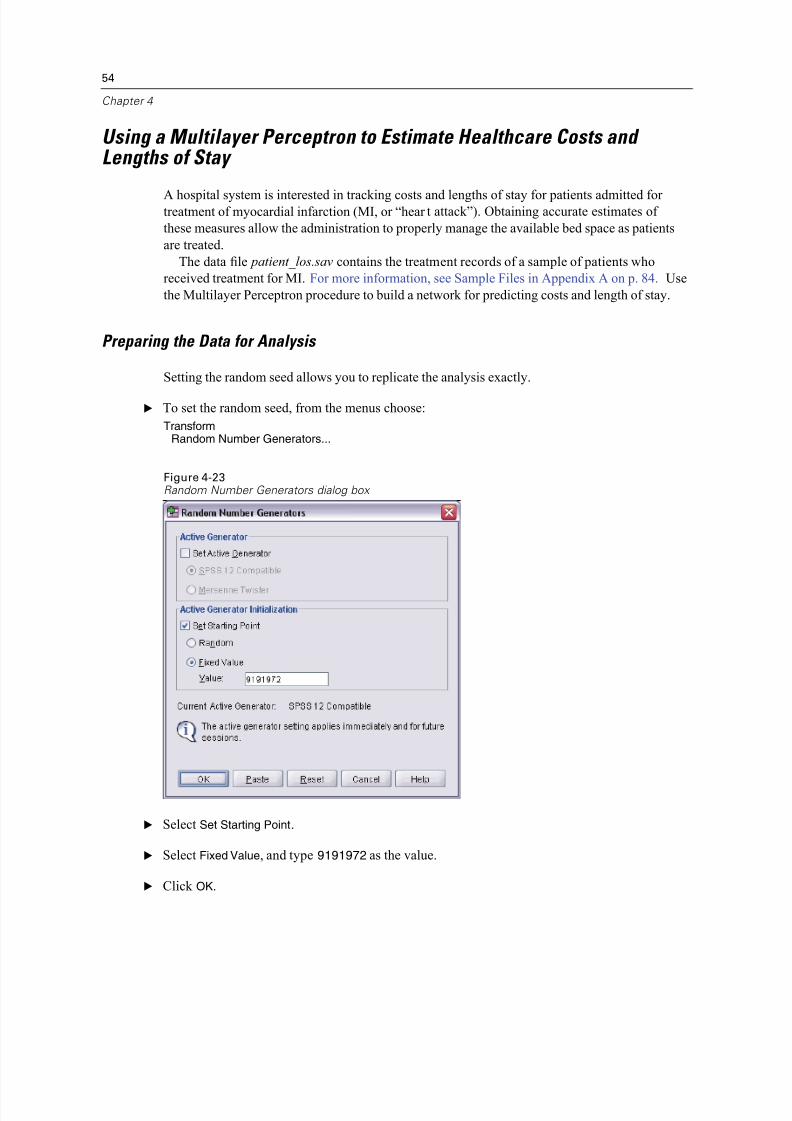
Setting the random seed allows you to replicate the analysis exactly.
E To set the random seed, from the menus choose:
TransformRandom Number Generators...
Figure 4-23Random Number Generators dialog box
E Select Set Starting Point.
E Select Fixed Value, and type 9191972 as the value.
E Click OK.
8/8/2019 SPSS Neural Network 16.0
http://slidepdf.com/reader/full/spss-neural-network-160 65/107
8/8/2019 SPSS Neural Network 16.0
http://slidepdf.com/reader/full/spss-neural-network-160 66/107
8/8/2019 SPSS Neural Network 16.0
http://slidepdf.com/reader/full/spss-neural-network-160 67/107
57
Multilayer Perceptron
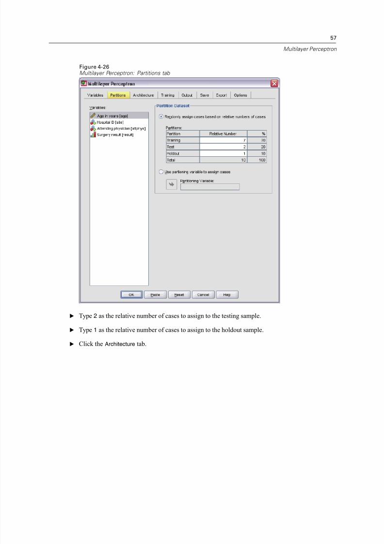
Figure 4-26Multilayer Perceptron: Partitions tab
E Type 2 as the relative number of cases to assign to the testing sample.
E Type 1 as the relative number of cases to assign to the holdout sample.
E Click the Architecture tab.

8/8/2019 SPSS Neural Network 16.0
http://slidepdf.com/reader/full/spss-neural-network-160 68/107
8/8/2019 SPSS Neural Network 16.0
http://slidepdf.com/reader/full/spss-neural-network-160 69/107
59
Multilayer Perceptron
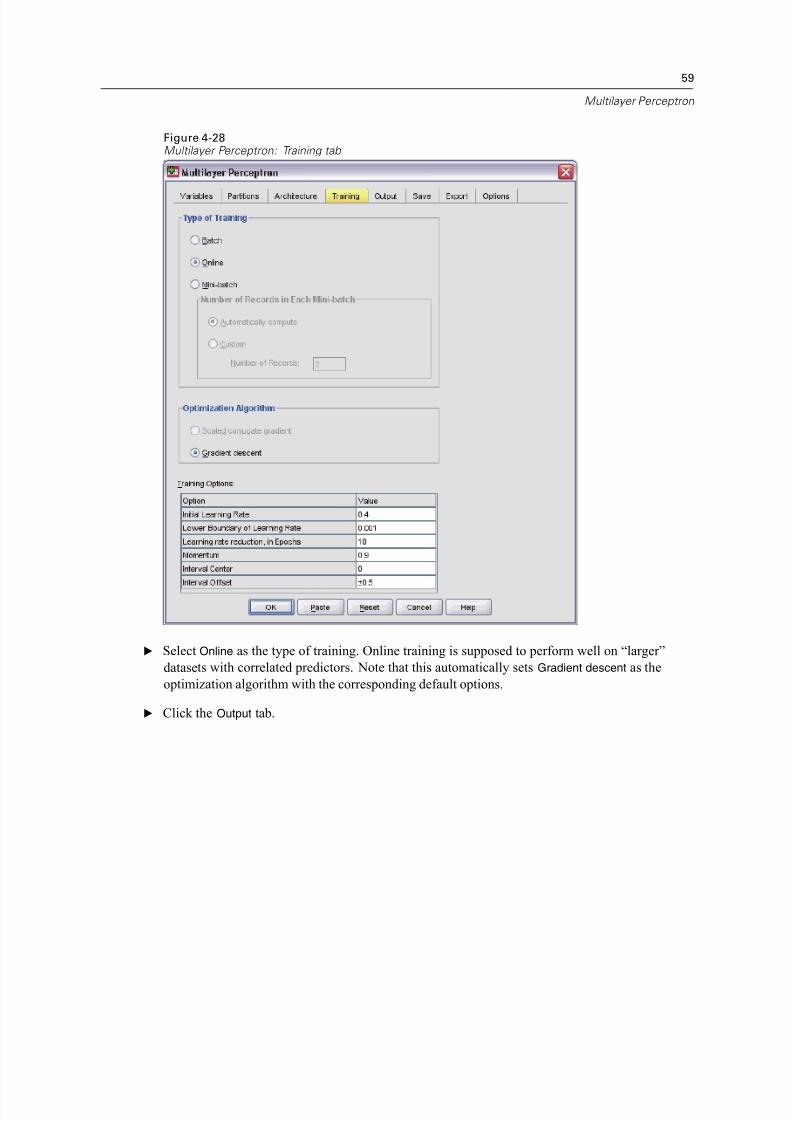
Figure 4-28Multilayer Perceptron: Training tab
E Select Online as the type of training. Online training is supposed to perform well on “larger”
datasets with correlated predictors. Note that this automatically sets Gradient descent as the
optimization algorithm with the corresponding default options.
E Click the Output tab.

8/8/2019 SPSS Neural Network 16.0
http://slidepdf.com/reader/full/spss-neural-network-160 70/107
8/8/2019 SPSS Neural Network 16.0
http://slidepdf.com/reader/full/spss-neural-network-160 71/107
61
Multilayer Perceptron
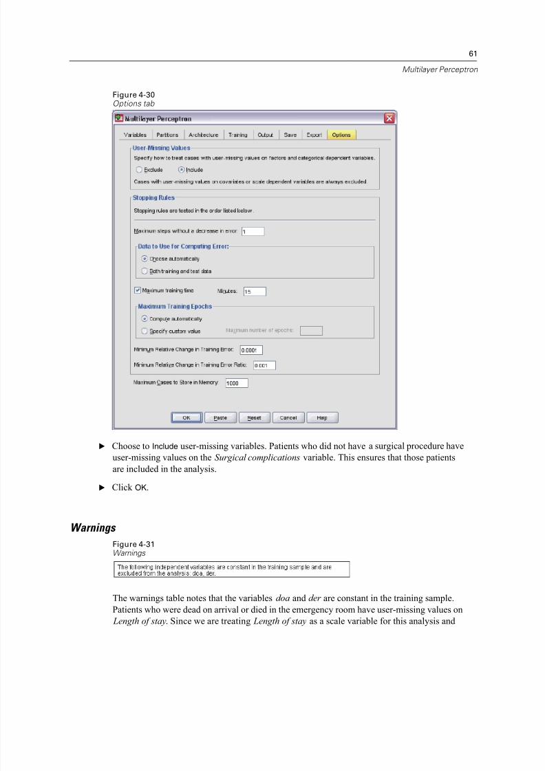
Figure 4-30Options tab
E Choose to Include user-missing variables. Patients who did not have a surgical procedure have
user-missing values on the Surgical complications variable. This ensures that those patients
are included in the analysis.
E Click OK.
Warnings
Figure 4-31Warnings
The warnings table notes that the variables doa and der are constant in the training sample.
Patients who were dead on arrival or died in the emergency room have user-missing values on
Length of stay. Since we are treating Length of stay as a scale variable for this analysis and

8/8/2019 SPSS Neural Network 16.0
http://slidepdf.com/reader/full/spss-neural-network-160 72/107

8/8/2019 SPSS Neural Network 16.0
http://slidepdf.com/reader/full/spss-neural-network-160 73/107
63
Multilayer Perceptron
Network Information
Figure 4-33Network information
The network information table displays information about the neural network and is useful for
ensur ing that the specifications are correct. Here, note in particular that:
The number of units in the input layer is the total number of factor levels (there are no
covariates).
Two hidden layers were requested, and the procedure has chosen 12 units in the first hiddenlayer and 9 in the second.
A separate output unit is created for each of the scale-dependent variables. They are rescaled
by the adjusted normalized method, which requires the use of the hyperbolic tangent
activation function for the output layer.
Sum-of-squares error is reported because the dependent variables are scale.

8/8/2019 SPSS Neural Network 16.0
http://slidepdf.com/reader/full/spss-neural-network-160 74/107
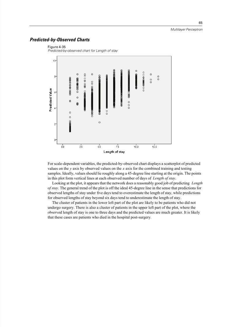
8/8/2019 SPSS Neural Network 16.0
http://slidepdf.com/reader/full/spss-neural-network-160 75/107
65
Multilayer Perceptron
Predicted-by-Observed Charts
Figure 4-35Predicted-by-observed chart for Length of stay
For scale-dependent variables, the predicted-by-observed chart displays a scatterplot of predicted
values on the y axis by observed values on the x axis for the combined training and testing
samples. Ideally, values should lie roughly along a 45-degree line starting at the origin. The points
in this plot form vertical lines at each observed number of days of Length of stay.
Looking at the plot, it appears that the network does a reasonably good job of predicting Length
of stay. The general trend of the plot is off the ideal 45-degree line in the sense that predictions for
observed lengths of stay under five days tend to overestimate the length of stay, while predictions
for observed lengths of stay beyond six days tend to underestimate the length of stay.
The cluster of patients in the lower left part of the plot are likely to be patients who did not
undergo surgery. There is also a cluster of patients in the upper left part of the plot, where the
observed length of stay is one to three days and the predicted values are much greater. It is likely
that these cases are patients who died in the hospital post-surgery.
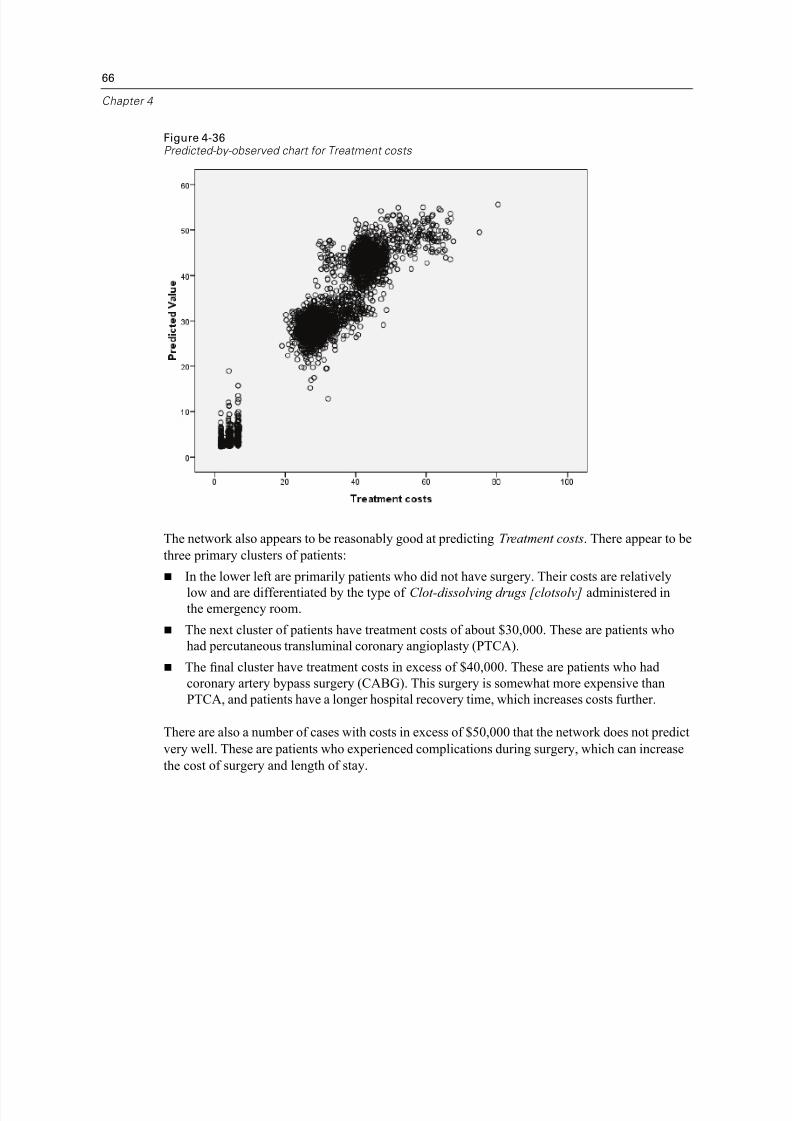
8/8/2019 SPSS Neural Network 16.0
http://slidepdf.com/reader/full/spss-neural-network-160 76/107
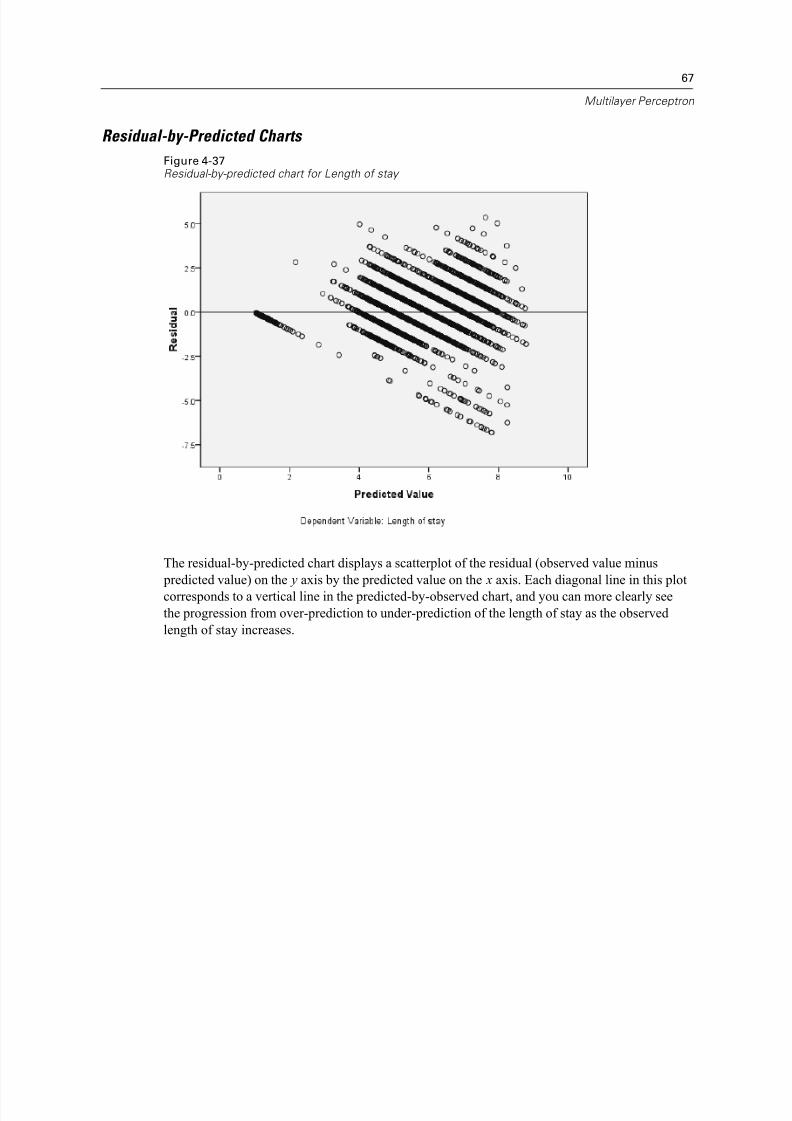
8/8/2019 SPSS Neural Network 16.0
http://slidepdf.com/reader/full/spss-neural-network-160 77/107
67
Multilayer Perceptron
Residual-by-Predicted Charts
Figure 4-37Residual-by-predicted chart for Length of stay
The residual-by-predicted chart displays a scatterplot of the residual (observed value minus
predicted value) on the y axis by the predicted value on the x axis. Each diagonal line in this plot
corresponds to a vertical line in the predicted-by-observed chart, and you can more clearly see
the progression from over-prediction to under-prediction of the length of stay as the observed
length of stay increases.
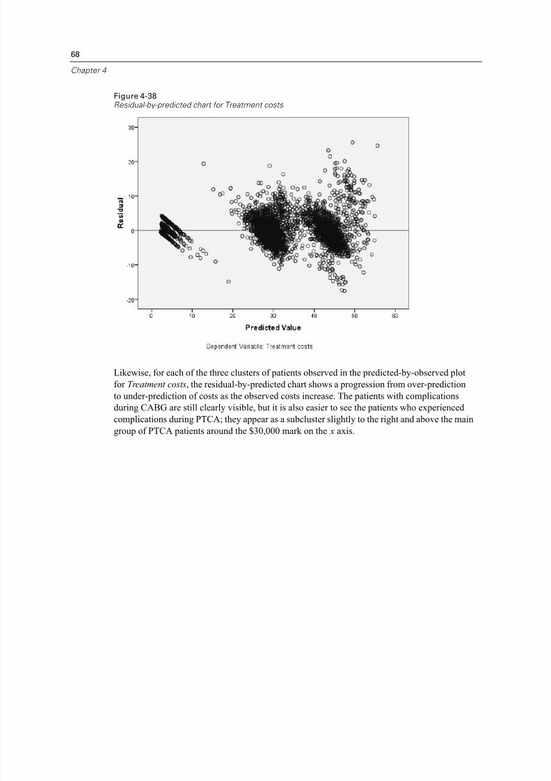
8/8/2019 SPSS Neural Network 16.0
http://slidepdf.com/reader/full/spss-neural-network-160 78/107
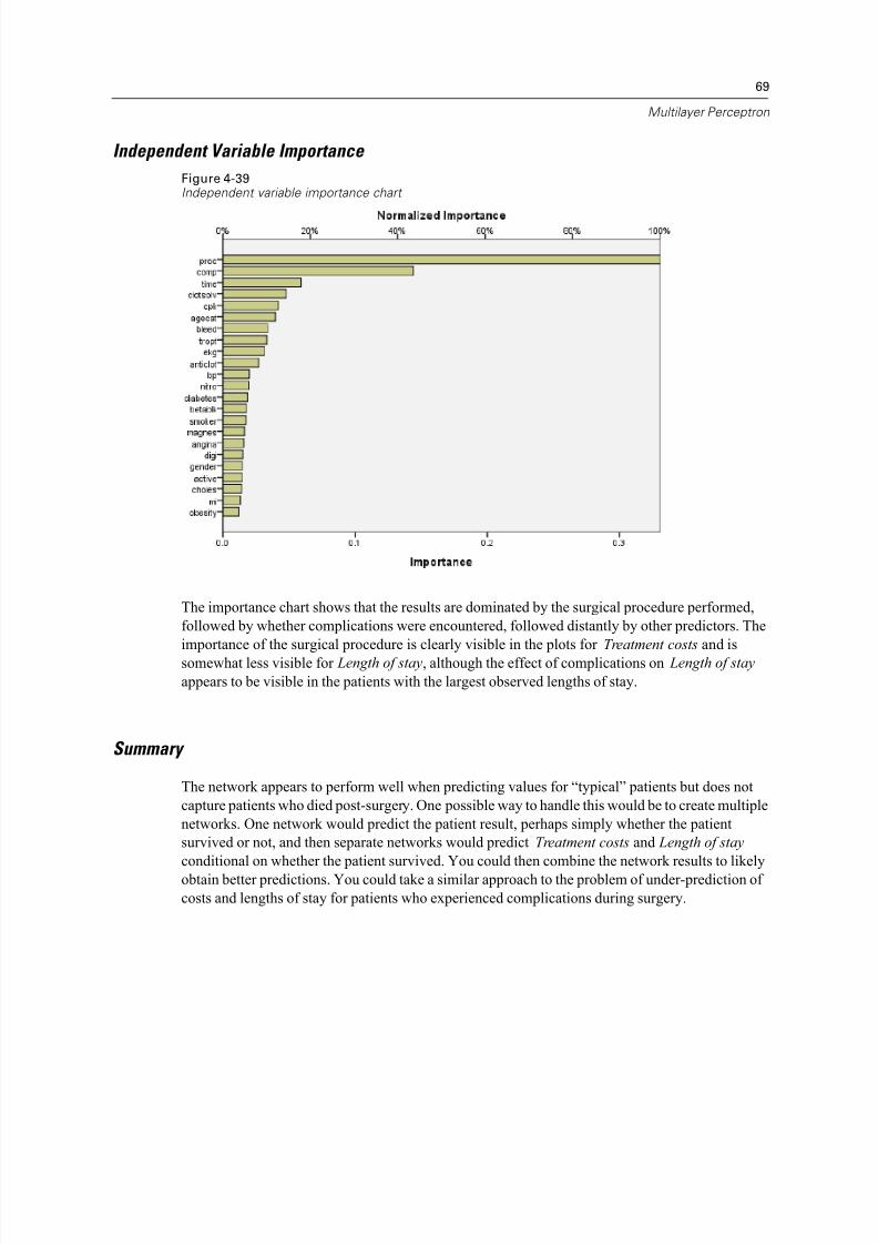
8/8/2019 SPSS Neural Network 16.0
http://slidepdf.com/reader/full/spss-neural-network-160 79/107

8/8/2019 SPSS Neural Network 16.0
http://slidepdf.com/reader/full/spss-neural-network-160 80/107
70
Chapter 4
Recommended Readings
See the following texts for more information on neural networks and multilayer perceptrons:
Bishop, C. M. 1995. Neural Networks for Pattern Recognition, 3rd ed. Oxford: Oxford University
Press.
Fine, T. L. 1999. Feedforward Neural Network Methodology, 3rd ed. New York: Springer-Verlag.
Haykin, S. 1998. Neural Networks: A Comprehensive Foundation, 2nd ed. New York: Macmillan
College Publishing.
Ripley, B. D. 1996. Pattern Recognition and Neural Networks. Cambridge: Cambridge University
Press.
8/8/2019 SPSS Neural Network 16.0
http://slidepdf.com/reader/full/spss-neural-network-160 81/107
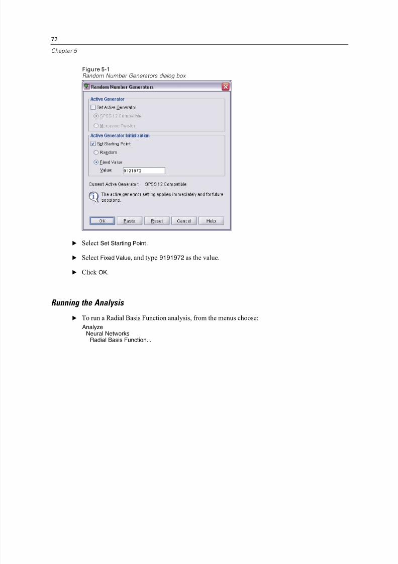
8/8/2019 SPSS Neural Network 16.0
http://slidepdf.com/reader/full/spss-neural-network-160 82/107
72
Chapter 5
Figure 5-1Random Number Generators dialog box
E Select Set Starting Point.
E Select Fixed Value, and type 9191972 as the value.
E Click OK.
Running the Analysis
E To run a Radial Basis Function analysis, from the menus choose:
AnalyzeNeural Networks
Radial Basis Function...

8/8/2019 SPSS Neural Network 16.0
http://slidepdf.com/reader/full/spss-neural-network-160 83/107
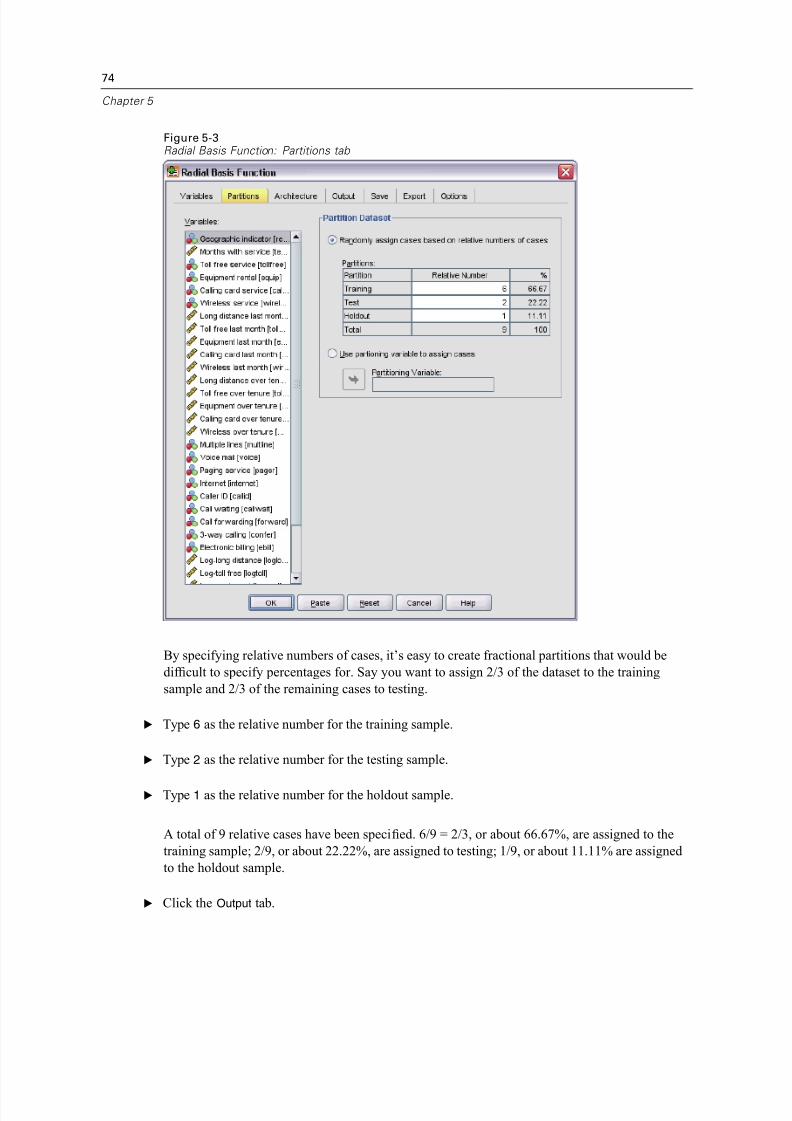
8/8/2019 SPSS Neural Network 16.0
http://slidepdf.com/reader/full/spss-neural-network-160 84/107
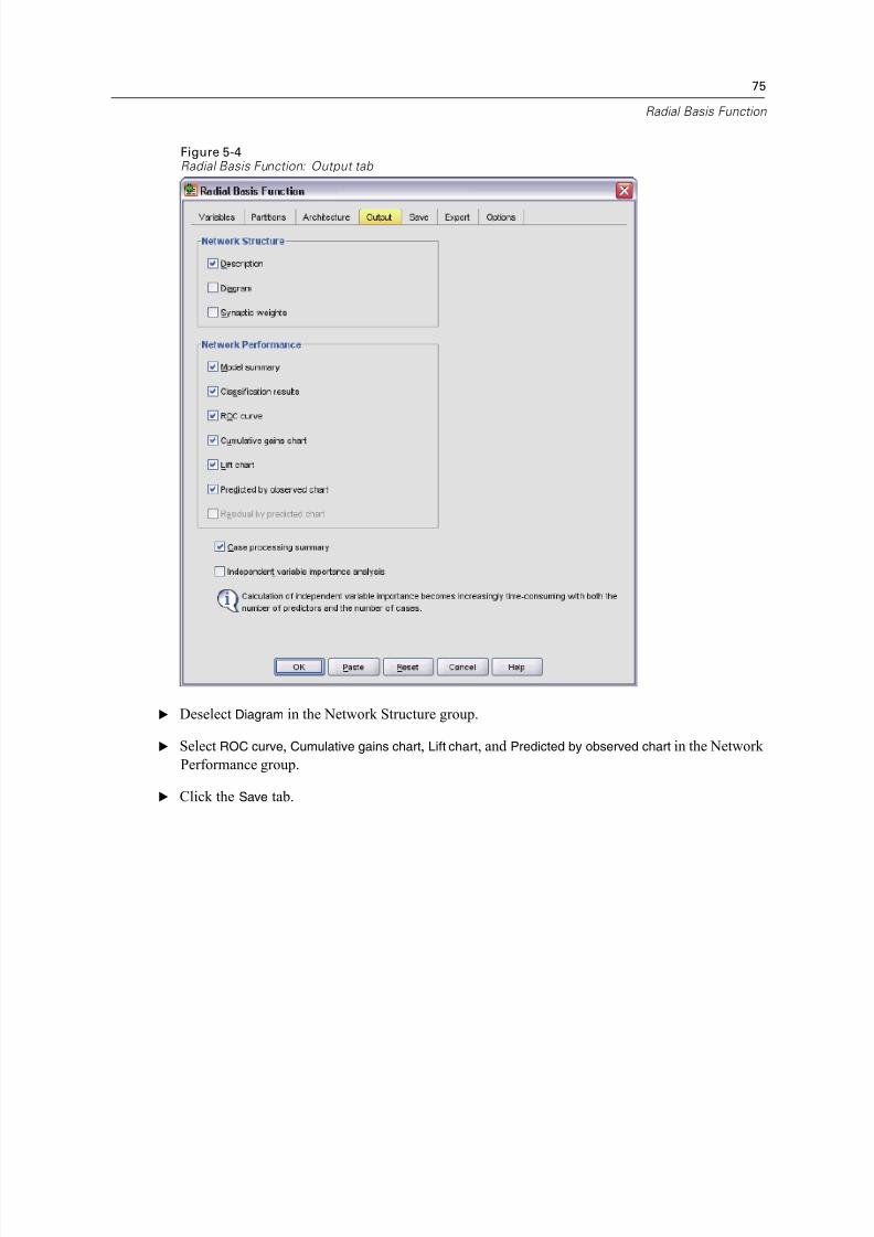
8/8/2019 SPSS Neural Network 16.0
http://slidepdf.com/reader/full/spss-neural-network-160 85/107

8/8/2019 SPSS Neural Network 16.0
http://slidepdf.com/reader/full/spss-neural-network-160 86/107

8/8/2019 SPSS Neural Network 16.0
http://slidepdf.com/reader/full/spss-neural-network-160 87/107

8/8/2019 SPSS Neural Network 16.0
http://slidepdf.com/reader/full/spss-neural-network-160 88/107

8/8/2019 SPSS Neural Network 16.0
http://slidepdf.com/reader/full/spss-neural-network-160 89/107
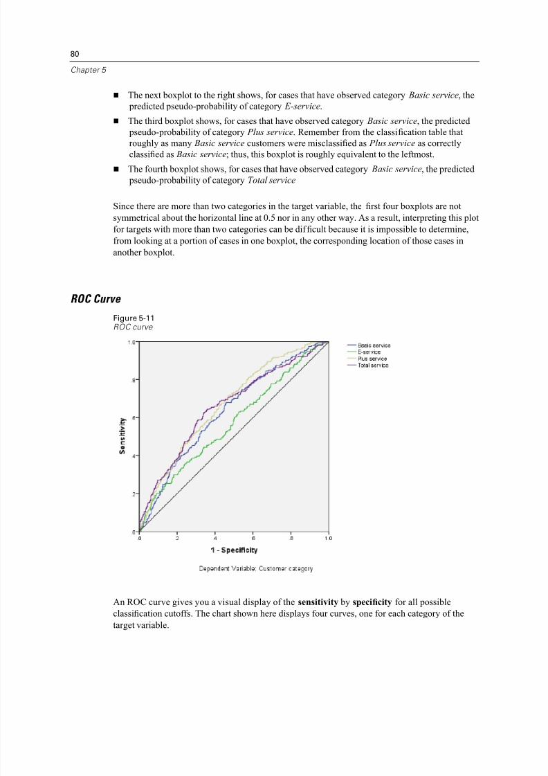
8/8/2019 SPSS Neural Network 16.0
http://slidepdf.com/reader/full/spss-neural-network-160 90/107
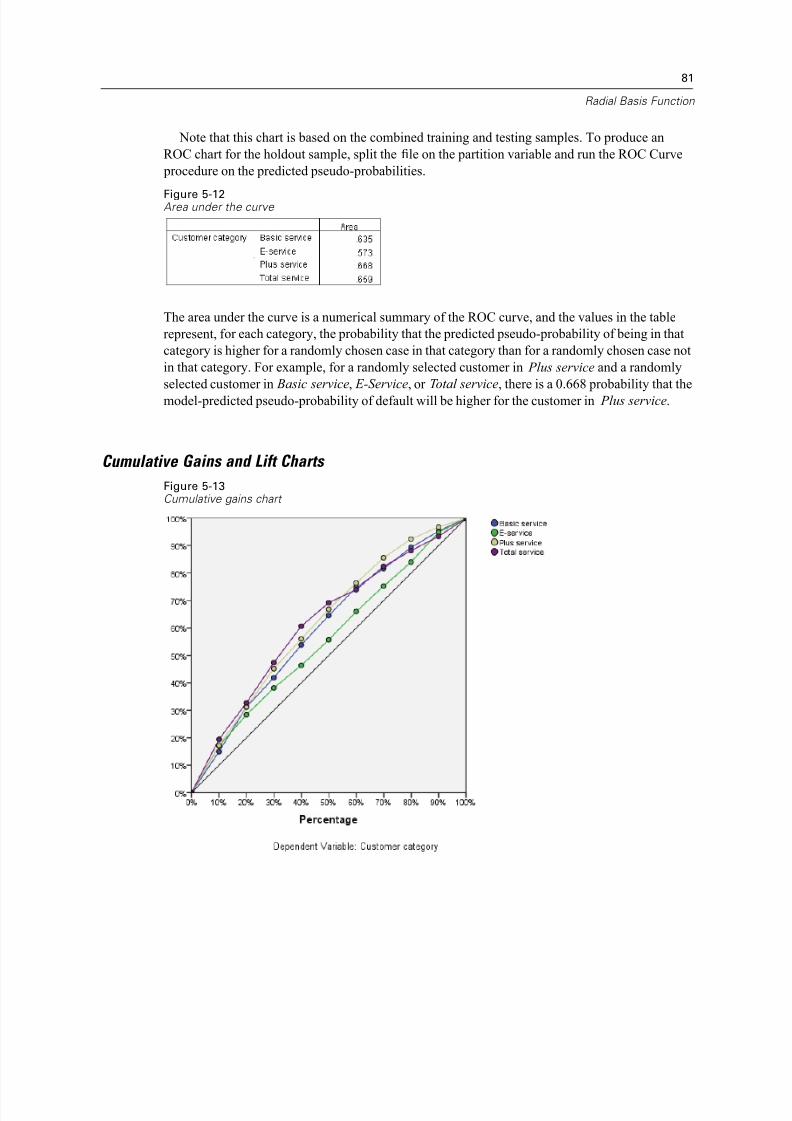
8/8/2019 SPSS Neural Network 16.0
http://slidepdf.com/reader/full/spss-neural-network-160 91/107

8/8/2019 SPSS Neural Network 16.0
http://slidepdf.com/reader/full/spss-neural-network-160 92/107

8/8/2019 SPSS Neural Network 16.0
http://slidepdf.com/reader/full/spss-neural-network-160 93/107
83
Radial Basis Function
Recommended Readings
See the following texts for more information on Radial Basis Function:
Bishop, C. M. 1995. Neural Networks for Pattern Recognition, 3rd ed. Oxford: Oxford University
Press.
Fine, T. L. 1999. Feedforward Neural Network Methodology, 3rd ed. New York: Springer-Verlag.
Haykin, S. 1998. Neural Networks: A Comprehensive Foundation, 2nd ed. New York: Macmillan
College Publishing.
Ripley, B. D. 1996. Pattern Recognition and Neural Networks. Cambridge: Cambridge University
Press.
Tao, K. K. 1993. A closer look at the radial basis function (RBF) networks. In: Conference Record of the Twenty-Seventh Asilomar Conference on Signals, Systems, and Computers, A.
Singh, ed. Los Alamitos,Calif.: IEEE Comput. Soc. Press, 401–405.
Uykan, Z., C. Guzelis, M. E. Celebi, and H. N. Koivo. 2000. Analysis of input-output clustering
for determining centers of RBFN. IEEE Transactions on Neural Networks, 11, 851–858.
8/8/2019 SPSS Neural Network 16.0
http://slidepdf.com/reader/full/spss-neural-network-160 94/107
Appendix
ASample Files
The sample files installed with the product can be found in the Samples subdirectory of the
installation directory.
Descriptions
Following are brief descriptions of the sample files used in various examples throughout the
documentation:
accidents.sav. This is a hypothetical data file that concerns an insurance company that is
studying age and gender risk factors for automobile accidents in a given region. Each case
corresponds to a cross-classification of age category and gender.
adl.sav. This is a hypothetical data file that concerns efforts to determine the benefits of a
proposed type of therapy for stroke patients. Physicians randomly assigned female stroke patients to one of two groups. The first received the standard physical therapy, and the second
received an additional emotional therapy. Three months following the treatments, each
patient’s abilities to perform common activities of daily life were scored as ordinal variables.
advert.sav. This is a hypothetical data file that concerns a retailer’s efforts to examine the
relationship between money spent on advertising and the resulting sales. To this end, they
have collected past sales figures and the associated advertising costs.. aflatoxin.sav. This is a hypothetical data file that concerns the testing of corn crops for
aflatoxin, a poison whose concentration varies widely between and within crop yields. A grain
processor has received 16 samples from each of 8 crop yields and measured the alfatoxin
levels in parts per billion (PPB).
aflatoxin20.sav. This data file contains the aflatoxin measurements from each of the 16 samples
from yields 4 and 8 from the a fl atoxin.sav data file.
anorectic.sav. While working toward a standardized symptomatology of anorectic/bulimic
behavior, researchers (Van der Ham, Meulman, Van Strien, and Van Engeland, 1997) made a
study of 55 adolescents with known eating disorders. Each patient was seen four times over
four years, for a total of 220 observations. At each observation, the patients were scored for
each of 16 symptoms. Symptom scores are missing for patient 71 at time 2, patient 76 at time2, and patient 47 at time 3, leaving 217 valid observations.
autoaccidents.sav. This is a hypothetical data file that concerns the efforts of an insurance
analyst to model the number of automobile accidents per driver while also accounting for
driver age and gender. Each case represents a separate driver and records the driver’s gender,
age in years, and number of automobile accidents in the last five years.
band.sav. This data file contains hypothetical weekly sales figures of music CDs for a band.
Data for three possible predictor variables are also included.
84

8/8/2019 SPSS Neural Network 16.0
http://slidepdf.com/reader/full/spss-neural-network-160 95/107
85
Sample Files
bankloan.sav. This is a hypothetical data file that concerns a bank’s efforts to reduce the
rate of loan defaults. The file contains financial and demographic information on 850 past
and prospective customers. The first 700 cases are customers who were previously given
loans. The last 150 cases are prospective customers that the bank needs to classify as good
or bad credit risks.
bankloan_binning.sav. This is a hypothetical data file containing financial and demographic
information on 5,000 past customers.
behavior.sav. In a classic example (Price and Bouffard, 1974), 52 students were asked to
rate the combinations of 15 situations and 15 behaviors on a 10-point scale ranging from
0=“extremely appropriate” to 9=“extremely inappropriate.” Averaged over individuals, the
values are taken as dissimilarities.
behavior_ini.sav. This data file contains an initial configuration for a two-dimensional solution
for behavior.sav.
brakes.sav. This is a hypothetical data file that concerns quality control at a factory that
produces disc brakes for high-performance automobiles. The data file contains diameter
measurements of 16 discs from each of 8 production machines. The target diameter for the
brakes is 322 millimeters.
breakfast.sav. In a classic study (Green and Rao, 1972), 21 Wharton School MBA students
and their spouses were asked to rank 15 breakfast items in order of preference with 1=“most
preferred” to 15=“least preferred.” Their preferences were recorded under six different
scenarios, from “Overall preference” to “Snack, with beverage only.”
breakfast-overall.sav. This data file contains the breakfast item preferences for the first
scenario, “Overall preference,” only.
broadband_1.sav. This is a hypothetical data file containing the number of subscribers, by
region, to a national broadband service. The data file contains monthly subscriber numbers
for 85 regions over a four-year period.
broadband_2.sav. This data file is identical to broadband_1.sav but contains data for three
additional months.
car_insurance_claims.sav. A dataset presented and analyzed elsewhere (McCullagh and
Nelder, 1989) concerns damage claims for cars. The average claim amount can be modeled
as having a gamma distribution, using an inverse link function to relate the mean of the
dependent variable to a linear combination of the policyholder age, vehicle type, and vehicle
age. The number of claims filed can be used as a scaling weight.
car_sales.sav. This data file contains hypothetical sales estimates, list prices, and physical
specifications for various makes and models of vehicles. The list prices and physical
specifications were obtained alternately from edmunds.com and manufacturer sites.
carpet.sav. In a popular example (Green and Wind, 1973), a company interested in
marketing a new carpet cleaner wants to examine the influence of five factors on consumer preference—package design, brand name, price, a Good Housekeeping seal, and a
money-back guarantee. There are three factor levels for package design, each one differing in
the location of the applicator brush; three brand names ( K2R, Glory, and Bissell ); three price
levels; and two levels (either no or yes) for each of the last two factors. Ten consumers rank
22 profiles defined by these factors. The variable Preference contains the rank of the average
rankings for each profile. Low rankings correspond to high preference. This variable reflects
an overall measure of preference for each profile.

8/8/2019 SPSS Neural Network 16.0
http://slidepdf.com/reader/full/spss-neural-network-160 96/107
86
Appendix A
carpet_prefs.sav. This data file is based on the same example as described for carpet.sav, but it
contains the actual rankings collected from each of the 10 consumers. The consumers were
asked to rank the 22 product profiles from the most to the least preferred. The variables PREF1 through PREF22 contain the identifiers of the associated profiles, as defined in
carpet_plan.sav.
catalog.sav. This data file contains hypothetical monthly sales figures for three products sold
by a catalog company. Data for five possible predictor variables are also included.
catalog_seasfac.sav. This data file is the same as catalog.sav except for the addition of a set
of seasonal factors calculated from the Seasonal Decomposition procedure along with the
accompanying date variables.
cellular.sav. This is a hypothetical data file that concerns a cellular phone company’s efforts
to reduce churn. Churn propensity scores are applied to accounts, ranging from 0 to 100.Accounts scoring 50 or above may be looking to change providers.
ceramics.sav. This is a hypothetical data file that concerns a manufacturer’s efforts to
determine whether a new premium alloy has a greater heat resistance than a standard alloy.
Each case represents a separate test of one of the alloys; the heat at which the bearing failed is
recorded.
cereal.sav. This is a hypothetical data file that concerns a poll of 880 people about their
breakfast preferences, also noting their age, gender, marital status, and whether or not they
have an active lifestyle (based on whether they exercise at least twice a week). Each case
represents a separate respondent.
clothing_defects.sav. This is a hypothetical data file that concerns the quality control process
at a clothing factory. From each lot produced at the factory, the inspectors take a sample of
clothes and count the number of clothes that are unacceptable.
coffee.sav. This data file pertains to perceived images of six iced-coffee brands (Kennedy,
Riquier, and Sharp, 1996) . For each of 23 iced-coffee image attributes, people selected all
brands that were described by the attribute. The six brands are denoted AA, BB, CC, DD, EE,and FF to preserve confidentiality.
contacts.sav. This is a hypothetical data file that concerns the contact lists for a group of
corporate computer sales representatives. Each contact is categorized by the department of
the company in which they work and their company ranks. Also recorded are the amount of
the last sale made, the time since the last sale, and the size of the contact’s company.
creditpromo.sav. This is a hypothetical data file that concerns a department store’s efforts to
evaluate the effectiveness of a recent credit card promotion. To this end, 500 cardholders were
randomly selected. Half received an ad promoting a reduced interest rate on purchases made
over the next three months. Half received a standard seasonal ad.
customer_dbase.sav. This is a hypothetical data file that concerns a company’s efforts to use
the information in its data warehouse to make special offers to customers who are mostlikely to reply. A subset of the customer base was selected at random and given the special
offers, and their responses were recorded.
customers_model.sav. This file contains hypothetical data on individuals targeted by a
marketing campaign. These data include demographic information, a summary of purchasing
history, and whether or not each individual responded to the campaign. Each case represents a
separate individual.

8/8/2019 SPSS Neural Network 16.0
http://slidepdf.com/reader/full/spss-neural-network-160 97/107
8/8/2019 SPSS Neural Network 16.0
http://slidepdf.com/reader/full/spss-neural-network-160 98/107
8/8/2019 SPSS Neural Network 16.0
http://slidepdf.com/reader/full/spss-neural-network-160 99/107
89
Sample Files
kinship_var.sav. This data file contains independent variables gender , gener (ation), and degree
(of separation) that can be used to interpret the dimensions of a solution for kinship_dat.sav.
Specifically, they can be used to restrict the space of the solution to a linear combination of
these variables.
mailresponse.sav. This is a hypothetical data file that concerns the efforts of a clothing
manufacturer to determine whether using first class postage for direct mailings results in
faster responses than bulk mail. Order-takers record how many weeks after the mailing
each order is taken.
marketvalues.sav. This data file concerns home sales in a new housing development in
Algonquin, Ill., during the years from 1999–2000. These sales are a matter of public record.
mutualfund.sav. This data file concerns stock market information for various tech stocks listed
on the S&P 500. Each case corresponds to a separate company.
nhis2000_subset.sav. The National Health Interview Survey (NHIS) is a large, population-based
survey of the U.S. civilian population. Interviews are carried out face-to-face in a nationally
representative sample of households. Demographic information and observations about
health behaviors and status are obtained for members of each household. This data
file contains a subset of information from the 2000 survey. National Center for Health
Statistics. National Health Interview Survey, 2000. Public-use data file and documentation. ftp://ftp.cdc.gov/pub/Health_Statistics/NCHS/Datasets/NHIS/2000/ . Accessed 2003.
ozone.sav. The data include 330 observations on six meteorological variables for predicting
ozone concentration from the remaining variables. Previous researchers (Breiman and
Friedman, 1985), (Hastie and Tibshirani, 1990), among others found nonlinearities among
these variables, which hinder standard regression approaches.
pain_medication.sav. This hypothetical data file contains the results of a clinical trial for
anti-inflammatory medication for treating chronic arthritic pain. Of particular interest is the
time it takes for the drug to take effect and how it compares to an existing medication.
patient_los.sav. This hypothetical data file contains the treatment records of patients who wereadmitted to the hospital for suspected myocardial infarction (MI, or “heart attack”). Each case
corresponds to a separate patient and records many variables related to their hospital stay.
patlos_sample.sav. This hypothetical data file contains the treatment records of a sample
of patients who received thrombolytics during treatment for myocardial infarction (MI, or
“heart attack”). Each case corresponds to a separate patient and records many variables
related to their hospital stay.
polishing.sav. This is the “Nambeware Polishing Times” data file from the Data and Story
Library. It concerns the efforts of a metal tableware manufacturer (Nambe Mills, Santa Fe, N.
M.) to plan its production schedule. Each case represents a different item in the product line.
The diameter, polishing time, price, and product type are recorded for each item.
poll_cs.sav. This is a hypothetical data file that concerns pollsters’ efforts to determine thelevel of public support for a bill before the legislature. The cases correspond to registered
voters. Each case records the county, township, and neighborhood in which the voter lives.
poll_cs_sample.sav. This hypothetical data file contains a sample of the voters listed in poll_cs.sav. The sample was taken according to the design specified in the poll.csplan plan
file, and this data file records the inclusion probabilities and sample weights. Note, however,
that because the sampling plan makes use of a probability-proportional-to-size (PPS) method,
there is also a file containing the joint selection probabilities ( poll_jointprob.sav). The

8/8/2019 SPSS Neural Network 16.0
http://slidepdf.com/reader/full/spss-neural-network-160 100/107
90
Appendix A
additional variables corresponding to voter demographics and their opinion on the proposed
bill were collected and added the data file after the sample as taken.
property_assess.sav. This is a hypothetical data file that concerns a county assessor’s efforts to
keep property value assessments up to date on limited resources. The cases correspond to properties sold in the county in the past year. Each case in the data file records the township
in which the property lies, the assessor who last visited the property, the time since that
assessment, the valuation made at that time, and the sale value of the property.
property_assess_cs.sav. This is a hypothetical data file that concerns a state assessor’s efforts
to keep property value assessments up to date on limited resources. The cases correspond
to properties in the state. Each case in the data file records the county, township, and
neighborhood in which the property lies, the time since the last assessment, and the valuation
made at that time.
property_assess_cs_sample.sav. This hypothetical data file contains a sample of the properties
listed in property_assess_cs.sav. The sample was taken according to the design specified in
the property_assess.csplan plan file, and this data file records the inclusion probabilities
and sample weights. The additional variable Current value was collected and added to thedata file after the sample was taken.
recidivism.sav. This is a hypothetical data file that concerns a government law enforcement
agency’s efforts to understand recidivism rates in their area of jurisdiction. Each case
corresponds to a previous offender and records their demographic information, some details
of their first crime, and then the time until their second arrest, if it occurred within two years
of the first arrest.
recidivism_cs_sample.sav. This is a hypothetical data file that concerns a government law
enforcement agency’s efforts to understand recidivism rates in their area of jurisdiction. Each
case corresponds to a previous offender, released from their first arrest during the month of
June, 2003, and records their demographic information, some details of their first crime, and
the data of their second arrest, if it occurred by the end of June, 2006. Offenders were selected
from sampled departments according to the sampling plan specified in recidivism_cs.csplan;
because it makes use of a probability-proportional-to-size (PPS) method, there is also a file
containing the joint selection probabilities (recidivism_cs_jointprob.sav).
salesperformance.sav. This is a hypothetical data file that concerns the evaluation of two
new sales training courses. Sixty employees, divided into three groups, all receive standard
training. In addition, group 2 gets technical training; group 3, a hands-on tutorial. Each
employee was tested at the end of the training course and their score recorded. Each case in
the data file represents a separate trainee and records the group to which they were assigned
and the score they received on the exam.
satisf.sav. This is a hypothetical data file that concerns a satisfaction survey conducted by
a retail company at 4 store locations. 582 customers were surveyed in all, and each case
represents the responses from a single customer. screws.sav. This data file contains information on the characteristics of screws, bolts, nuts,
and tacks (Hartigan, 1975).
shampoo_ph.sav. This is a hypothetical data file that concerns the quality control at a factory
for hair products. At regular time intervals, six separate output batches are measured and their
pH recorded. The target range is 4.5–5.5.
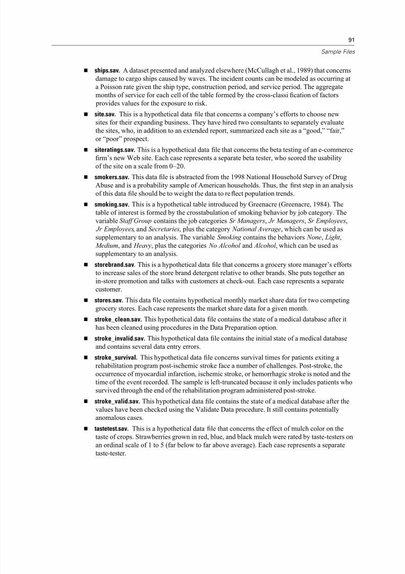
8/8/2019 SPSS Neural Network 16.0
http://slidepdf.com/reader/full/spss-neural-network-160 101/107

8/8/2019 SPSS Neural Network 16.0
http://slidepdf.com/reader/full/spss-neural-network-160 102/107
92
Appendix A
telco.sav. This is a hypothetical data file that concerns a telecommunications company’s
efforts to reduce churn in their customer base. Each case corresponds to a separate customer
and records various demographic and service usage information.
telco_extra.sav. This datafi
le is similar to the telco.sav datafi
le, but the “tenure” andlog-transformed customer spending variables have been removed and replaced by
standardized log-transformed customer spending variables.
telco_missing.sav. This data file is the same as the telco_mva_complete.sav data file, but some
of the data have been replaced with missing values.
telco_mva_complete.sav. This data file is a subset of the telco.sav data file but with different
variable names.
testmarket.sav. This hypothetical data file concerns a fast food chain’s plans to add a new item
to its menu. There are three possible campaigns for promoting the new product, so the new
item is introduced at locations in several randomly selected markets. A different promotion
is used at each location, and the weekly sales of the new item are recorded for the first four
weeks. Each case corresponds to a separate location-week.
testmarket_1month.sav. This hypothetical data file is the testmarket.sav data file with the
weekly sales “rolled-up” so that each case corresponds to a separate location. Some of the
variables that changed weekly disappear as a result, and the sales recorded is now the sum of
the sales during the four weeks of the study.
tree_car.sav. This is a hypothetical data file containing demographic and vehicle purchase
price data.
tree_credit.sav. This is a hypothetical data file containing demographic and bank loan history
data.
tree_missing_data.sav This is a hypothetical data file containing demographic and bank loan
history data with a large number of missing values.
tree_score_car.sav. This is a hypothetical data file containing demographic and vehicle purchase price data.
tree_textdata.sav. A simple data file with only two variables intended primarily to show the
default state of variables prior to assignment of measurement level and value labels.
tv-survey.sav. This is a hypothetical data file that concerns a survey conducted by a TV studio
that is considering whether to extend the run of a successful program. 906 respondents were
asked whether they would watch the program under various conditions. Each row represents a
separate respondent; each column is a separate condition.
ulcer_recurrence.sav. This file contains partial information from a study designed to compare
the ef ficacy of two therapies for preventing the recurrence of ulcers. It provides a good
example of interval-censored data and has been presented and analyzed elsewhere (Collett,
2003).
ulcer_recurrence_recoded.sav. This file reorganizes the information in ulcer_recurrence.sav to
allow you model the event probability for each interval of the study rather than simply the
end-of-study event probability. It has been presented and analyzed elsewhere (Collett etal., 2003).
verd1985.sav. This data file concerns a survey (Verdegaal, 1985). The responses of 15 subjects
to 8 variables were recorded. The variables of interest are divided into three sets. Set 1
includes age and marital , set 2 includes pet and news, and set 3 includes music and live.
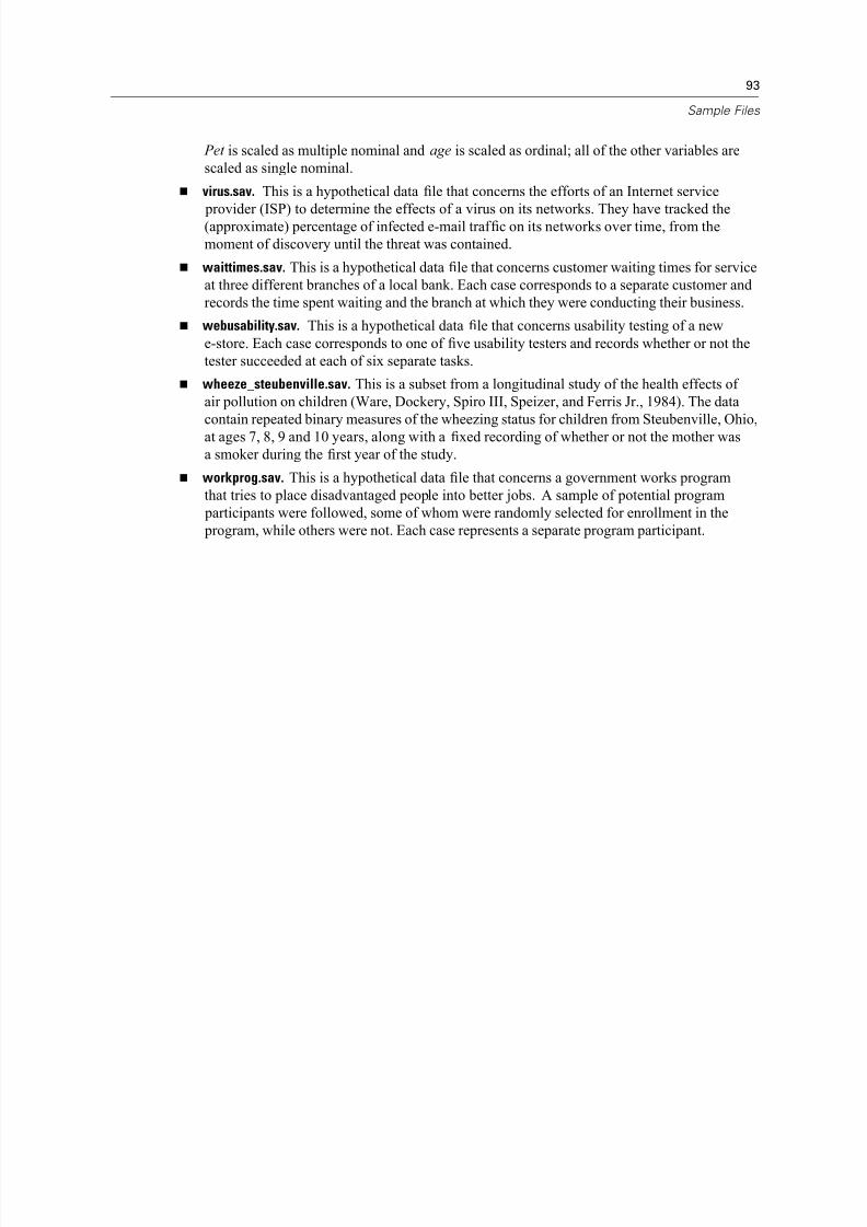
8/8/2019 SPSS Neural Network 16.0
http://slidepdf.com/reader/full/spss-neural-network-160 103/107
93
Sample Files
Pet is scaled as multiple nominal and age is scaled as ordinal; all of the other variables are
scaled as single nominal.
virus.sav. This is a hypothetical data file that concerns the efforts of an Internet service
provider (ISP) to determine the effects of a virus on its networks. They have tracked the(approximate) percentage of infected e-mail traf fic on its networks over time, from the
moment of discovery until the threat was contained.
waittimes.sav. This is a hypothetical data file that concerns customer waiting times for service
at three different branches of a local bank. Each case corresponds to a separate customer and
records the time spent waiting and the branch at which they were conducting their business.
webusability.sav. This is a hypothetical data file that concerns usability testing of a new
e-store. Each case corresponds to one of five usability testers and records whether or not the
tester succeeded at each of six separate tasks.
wheeze_steubenville.sav. This is a subset from a longitudinal study of the health effects of
air pollution on children (Ware, Dockery, Spiro III, Speizer, and Ferris Jr., 1984). The data
contain repeated binary measures of the wheezing status for children from Steubenville, Ohio,
at ages 7, 8, 9 and 10 years, along with a fixed recording of whether or not the mother was
a smoker during the first year of the study.
workprog.sav. This is a hypothetical data file that concerns a government works program
that tries to place disadvantaged people into better jobs. A sample of potential program
participants were followed, some of whom were randomly selected for enrollment in the
program, while others were not. Each case represents a separate program participant.

8/8/2019 SPSS Neural Network 16.0
http://slidepdf.com/reader/full/spss-neural-network-160 104/107

8/8/2019 SPSS Neural Network 16.0
http://slidepdf.com/reader/full/spss-neural-network-160 105/107
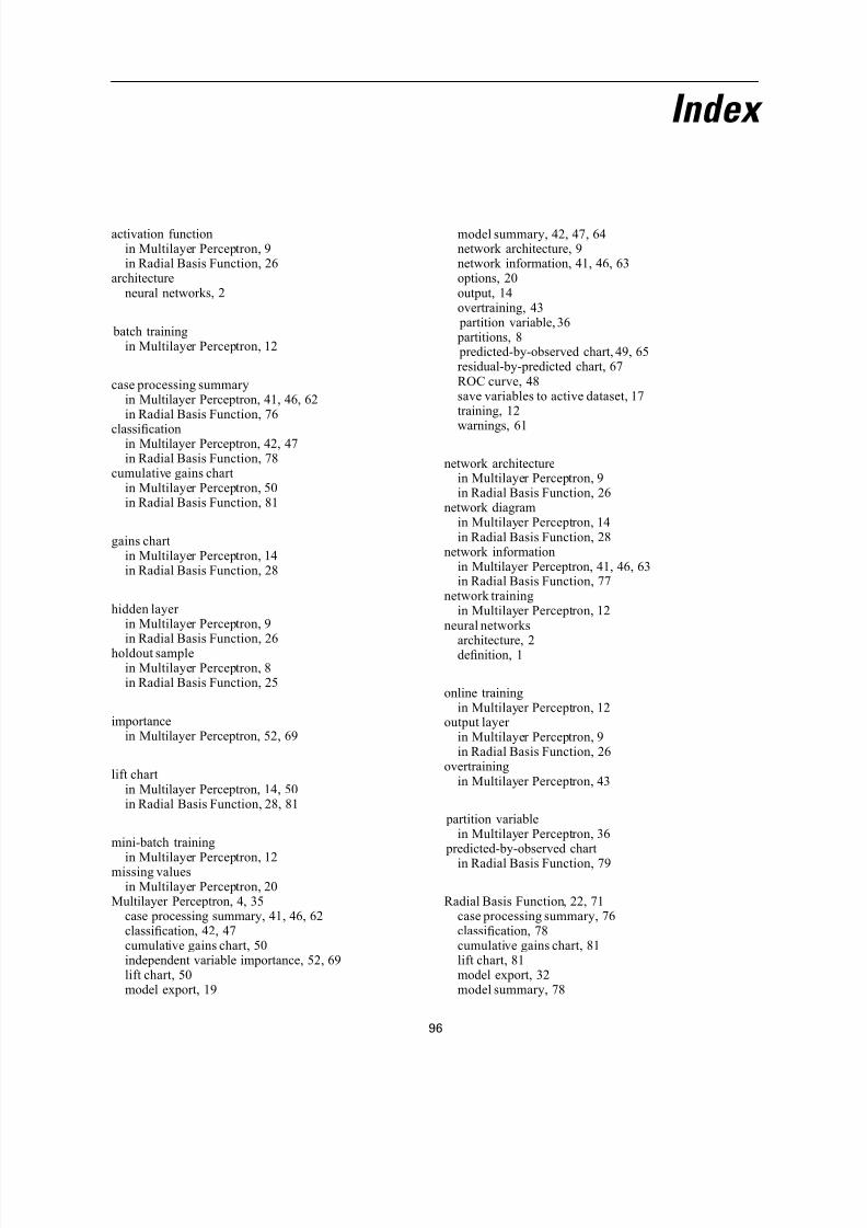
8/8/2019 SPSS Neural Network 16.0
http://slidepdf.com/reader/full/spss-neural-network-160 106/107

8/8/2019 SPSS Neural Network 16.0
http://slidepdf.com/reader/full/spss-neural-network-160 107/107