SPSS Conjoint

8/7/2019 SPSS Conjoint

1/63

i

SPSSConjoint

17.0


2/63

For more information about SPSS Inc. software products, please visit our Web site at http://www.spss.com or contact

SPSS Inc.

233 South Wacker Drive, 11th Floor

Chicago, IL 60606-6412

Tel: (312) 651-3000

Fax: (312) 651-3668

SPSS is a registered trademark and the other product names are the trademarks of SPSS Inc. for its proprietary comp

software. No material describing such software may be produced or distributed without the written permission of the

owners of the trademark and license rights in the software and the copyrights in the published materials.

The SOFTWARE and documentation are provided with RESTRICTED RIGHTS. Use, duplication, or disclosure by

the Government is subject to restrictions as set forth in subdivision (c) (1) (ii) of The Rights in Technical Data and

Computer Software clause at 52.227-7013. Contractor/manufacturer is SPSS Inc., 233 South Wacker Drive, 11th

Floor, Chicago, IL 60606-6412.

Patent No. 7,023,453

General notice: Other product names mentioned herein are used for identification purposes only and may be tradema

of their respective companies.

Windows is a registered trademark of Microsoft Corporation.

Apple, Mac, and the Mac logo are trademarks of Apple Computer, Inc., registered in the U.S. and other countries.

This product uses WinWrap Basic, Copyright 1993-2007, Polar Engineering and Consulting, http://www.winwrap.co

Printed in the United States of America.

No part of this publication may be reproduced, stored in a retrieval system, or transmitted, in any form or by any mea

electronic, mechanical, photocopying, recording, or otherwise, without the prior written permission of the publisher.


3/63

Preface

SPSS Statistics 17.0 is a comprehensive system for analyzing data. The Conjoint

optional add-on module provides the additional analytic techniques described in this

manual. The Conjoint add-on module must be used with the SPSS Statistics 17.0 Base

system and is completely integrated into that system.

Installation

To install the Conjoint add-on module, run the License Authorization Wizard using the

authorization code that you received from SPSS Inc. For more information, see the

installation instructions supplied with the Conjoint add-on module.

Compatibility

SPSS Statistics is designed to run on many computer systems. See the installation

instructions that came with your system for specific information on minimum and

recommended requirements.

Serial Numbers

Your serial number is your identification number with SPSS Inc. You will need this

serial number when you contact SPSS Inc. for information regarding support, payment

or an upgraded system. The serial number was provided with your Base system.

Customer Service

If you have any questions concerning your shipment or account, contact your local

office, listed on the Web site at http://www.spss.com/worldwide . Please have your

serial number ready for identification.

iii


4/63

Training Seminars

SPSS Inc. provides both public and onsite training seminars. All seminars feature

hands-on workshops. Seminars will be offered in major cities on a regular basis.

For more information on these seminars, contact your local office, listed on the Website at http://www.spss.com/worldwide .

Technical Support

Technical Support services are available to maintenance customers. Customers may

contact Technical Support for assistance in using SPSS Statistics or for installation

help for one of the supported hardware environments. To reach Technical Support,

see the Web site at http://www.spss.com, or contact your local office, listed on the

Web site at http://www.spss.com/worldwide . Be prepared to identify yourself, your

organization, and the serial number of your system.

Additional Publications

The SPSS Statistical Procedures Companion, by Marija Noruis, has been published

by Prentice Hall. A new version of this book, updated for SPSS Statistics 17.0,

is planned. The SPSS Advanced Statistical Procedures Companion, also based

on SPSS Statistics 17.0, is forthcoming. The SPSS Guide to Data Analysis for

SPSS Statistics 17.0 is also in development. Announcements of publications

available exclusively through Prentice Hall will be available on the Web site at

http://www.spss.com/estore (select your home country, and then clickBooks).

iv


5/63

Contents

1 Introduction to Conjoint Analysis 1

The Full-Profile Approach . . . . . . . . . . . . . . . . . . . . . . . . . . . . . . . . . . . . . . . . 2

An Orthogonal Array . . . . . . . . . . . . . . . . . . . . . . . . . . . . . . . . . . . . . . . . 2

The Experimental Stimuli . . . . . . . . . . . . . . . . . . . . . . . . . . . . . . . . . . . . . 3

Collecting and Analyzing the Data . . . . . . . . . . . . . . . . . . . . . . . . . . . . . . 3

Part I: User's Guide

2 Generating an Orthogonal Design 6

Defining Values for an Orthogonal Design . . . . . . . . . . . . . . . . . . . . . . . . . . . . 8

Orthogonal Design Options . . . . . . . . . . . . . . . . . . . . . . . . . . . . . . . . . . . . . . . 9

ORTHOPLAN Command Additional Features . . . . . . . . . . . . . . . . . . . . . . . . . 10

3 Displaying a Design 11

Display Design Titles. . . . . . . . . . . . . . . . . . . . . . . . . . . . . . . . . . . . . . . . . . . 12

PLANCARDS Command Additional Features . . . . . . . . . . . . . . . . . . . . . . . . . 13

v


6/63

4 Running a Conjoint Analysis 14

Requirements . . . . . . . . . . . . . . . . . . . . . . . . . . . . . . . . . . . . . . . . . . . . . . . 14

Specifying the Plan File and the Data File. . . . . . . . . . . . . . . . . . . . . . . . 15

Specifying How Data Were Recorded . . . . . . . . . . . . . . . . . . . . . . . . . . 15

Optional Subcommands . . . . . . . . . . . . . . . . . . . . . . . . . . . . . . . . . . . . . . . . 17

Part II: Examples

5 Using Conjoint Analysis to Model Carpet-CleanerPreference 21

Generating an Orthogonal Design . . . . . . . . . . . . . . . . . . . . . . . . . . . . . . . . . 22

Creating the Experimental Stimuli: Displaying the Design . . . . . . . . . . . . . . . 26

Running the Analysis . . . . . . . . . . . . . . . . . . . . . . . . . . . . . . . . . . . . . . . . . . 29

Utility Scores . . . . . . . . . . . . . . . . . . . . . . . . . . . . . . . . . . . . . . . . . . . . . . . . 32

Coefficients . . . . . . . . . . . . . . . . . . . . . . . . . . . . . . . . . . . . . . . . . . . . . . . . . 33

Relative Importance . . . . . . . . . . . . . . . . . . . . . . . . . . . . . . . . . . . . . . . . . . . 33

Correlations . . . . . . . . . . . . . . . . . . . . . . . . . . . . . . . . . . . . . . . . . . . . . . . . . 34

Reversals . . . . . . . . . . . . . . . . . . . . . . . . . . . . . . . . . . . . . . . . . . . . . . . . . . . 35

Running Simulations . . . . . . . . . . . . . . . . . . . . . . . . . . . . . . . . . . . . . . . . . . . 35

Preference Probabilities of Simulations . . . . . . . . . . . . . . . . . . . . . . . . . . . . 37

vi


7/63

Appendix

A Sample Files 38

Bibliography 52

Index 54

vii


8/63


9/63

Chapte1Introduction to Conjoint Analysis

Conjoint analysis is a market research tool for developing effective product design.

Using conjoint analysis, the researcher can answer questions such as: What product

attributes are important or unimportant to the consumer? What levels of product

attributes are the most or least desirable in the consumers mind? What is the market

share of preference for leading competitors products versus our existing or proposedproduct?

The virtue of conjoint analysis is that it asks the respondent to make choices in the

same fashion as the consumer presumably doesby trading off features, one against

another.

For example, suppose that you want to book an airline flight. You have the choice

of sitting in a cramped seat or a spacious seat. If this were the only consideration, your

choice would be clear. You would probably prefer a spacious seat. Or suppose you

have a choice of ticket prices: $225 or $800. On price alone, taking nothing else into

consideration, the lower price would be preferable. Finally, suppose you can take

either a directfl

ight, which takes two hours, or afl

ight with one layover, which takesfive hours. Most people would choose the direct flight.

The drawback to the above approach is that choice alternatives are presented on

single attributes alone, one at a time. Conjoint analysis presents choice alternatives

between products defined by sets of attributes. This is illustrated by the following

choice: would you prefer a flight that is cramped, costs $225, and has one layover, or a

flight that is spacious, costs $800, and is direct? If comfort, price, and duration are the

relevant attributes, there are potentially eight products:

Product Comfort Price Duration

1 cramped $225 2 hours




1


10/63

2

Chapter 1

Product Comfort Price Duration

5 spacious $225 2 hours




Given the above alternatives, product 4 is probably the least preferred, while product 5

is probably the most preferred. The preferences of respondents for the other product

offerings are implicitly determined by what is important to the respondent.

Using conjoint analysis, you can determine both the relative importance of each

attribute as well as which levels of each attribute are most preferred. If the most

preferable product is not feasible for some reason, such as cost, you would know the

next most preferred alternative. If you have other information on the respondents,such as background demographics, you might be able to identify market segments

for which distinct products can be packaged. For example, the business traveler and

the student traveler might have different preferences that could be met by distinct

product offerings.

The Full-Profile Approach

Conjoint uses the full-profile (also known as full-concept) approach, where

respondents rank, order, or score a set of profiles, or cards, according to preference.

Each profile describes a complete product or service and consists of a differentcombination of factor levels for all factors (attributes) of interest.

An Orthogonal Array

A potential problem with the full-profile approach soon becomes obvious if more than

a few factors are involved and each factor has more than a couple of levels. The total

number of profiles resulting from all possible combinations of the levels becomes too

great for respondents to rank or score in a meaningful way. To solve this problem, the

full-profi

le approach uses what is termed a fractional factorial design, which presenta suitable fraction of all possible combinations of the factor levels. The resulting set,

called an orthogonal array, is designed to capture the main effects for each factor

level. Interactions between levels of one factor with levels of another factor are

assumed to be negligible.


11/63

3

Introduction to Conjoint Analysis

The Generate Orthogonal Design procedure is used to generate an orthogonal array

and is typically the starting point of a conjoint analysis. It also allows you to generate

factor-level combinations, known as holdout cases, which are rated by the subjects

but are not used to build the preference model. Instead, they are used as a check on

the validity of the model.

The Experimental Stimuli

Each set of factor levels in an orthogonal design represents a different version of the

product under study and should be presented to the subjects in the form of an individua

product profile. This helps the respondent to focus on only the one product currently

under evaluation. The stimuli should be standardized by making sure that the profiles

are all similar in physical appearance except for the different combinations of featuresCreation of the product profiles is facilitated with the Display Design procedure. It

takes a design generated by the Generate Orthogonal Design procedure, or entered by

the user, and produces a set of product profiles in a ready-to-use format.

Collecting and Analyzing the Data

Since there is typically a great deal of between-subject variation in preferences, much

of conjoint analysis focuses on the single subject. To generalize the results, a random

sample of subjects from the target population is selected so that group results canbe examined.

The size of the sample in conjoint studies varies greatly. In one report (Cattin and

Wittink, 1982), the authors state that the sample size in commercial conjoint studies

usually ranges from 100 to 1,000, with 300 to 550 the most typical range. In another

study (Akaah and Korgaonkar, 1988), it is found that smaller sample sizes (less

than 100) are typical. As always, the sample size should be large enough to ensure

reliability.

Once the sample is chosen, the researcher administers the set of profiles, or cards, to

each respondent. The Conjoint procedure allows for three methods of data recording.

In thefi

rst method, subjects are asked to assign a preference score to each profi

le.This type of method is typical when a Likert scale is used or when the subjects are

asked to assign a number from 1 to 100 to indicate preference. In the second method,

subjects are asked to assign a rank to each profile ranging from 1 to the total number

of profiles. In the third method, subjects are asked to sort the profiles in terms of


12/63

4

Chapter 1

preference. With this last method, the researcher records the profile numbers in the

order given by each subject.

Analysis of the data is done with the Conjoint procedure (available only through

command syntax) and results in a utility score, called a part-worth, for each factor

level. These utility scores, analogous to regression coefficients, provide a quantitative

measure of the preference for each factor level, with larger values corresponding to

greater preference. Part-worths are expressed in a common unit, allowing them to be

added together to give the total utility, or overall preference, for any combination of

factor levels. The part-worths then constitute a model for predicting the preference

of any product profile, including profiles, referred to as simulation cases, that were

not actually presented in the experiment.

The information obtained from a conjoint analysis can be applied to a wide variety

of market research questions. It can be used to investigate areas such as product design

market share, strategic advertising, cost-benefit analysis, and market segmentation.Although the focus of this manual is on market research applications, conjoint

analysis can be useful in almost any scientific or business field in which measuring

peoples perceptions or judgments is important.


13/63

Part I:User's Guide


14/63

Chapte2Generating an Orthogonal Design

Generate Orthogonal Design generates a data file containing an orthogonal main-effect

design that permits the statistical testing of several factors without testing every

combination of factor levels. This design can be displayed with the Display Design

procedure, and the data file can be used by other procedures, such as Conjoint.

Example. A low-fare airline startup is interested in determining the relative importance

to potential customers of the various factors that comprise its product offering. Price is

clearly a primary factor, but how important are other factors, such as seat size, number

of layovers, and whether or not a beverage/snack service is included? A survey asking

respondents to rank product profiles representing all possible factor combinations is

unreasonable given the large number of profiles. The Generate Orthogonal Design

procedure creates a reduced set of product profiles that is small enough to include in a

survey but large enough to assess the relative importance of each factor.

To Generate an Orthogonal Design

E From the menus choose:

DataOrthogonal Design

Generate...

6


15/63

7

Generating an Orthogonal Design

Figure 2-1Generate Orthogonal Design dialog box

E Define at least one factor. Enter a name in the Factor Name text box. Factor names

can be any valid variable name, except status_ orcard_. You can also assign an

optional factor label.

E ClickAdd to add the factor name and an optional label. To delete a factor, select it in

the list and clickRemove. To modify a factor name or label, select it in the list, modify

the name or label, and click Change.

E Define values for each factor by selecting the factor and clicking Define Values.

Data File. Allows you to control the destination of the orthogonal design. You can save

the design to a new dataset in the current session or to an external data file.

Create a new dataset. Creates a new dataset in the current session containing the

factors and cases generated by the plan.

Create new data file. Creates an external data file containing the factors and cases

generated by the plan. By default, this data file is named ortho.sav, and it is saved

to the current directory. ClickFile to specify a different name and destination for

the file.


16/63

8

Chapter 2

Reset random number seed to. Resets the random number seed to the specified value.

The seed can be any integer value from 0 through 2,000,000,000. Within a session,

a different seed is used each time you generate a set of random numbers, producing

different results. If you want to duplicate the same random numbers, you should set the

seed value before you generate yourfirst design and reset the seed to the same value

each subsequent time you generate the design.

Optionally, you can:

ClickOptions to specify the minimum number of cases in the orthogonal design

and to select holdout cases.

Defining Values for an Orthogonal Design

Figure 2-2Generate Design Define Values dialog box

You must assign values to each level of the selected factor or factors. The factor name

will be displayed afterValues and Labels for.Enter each value of the factor. You can elect to give the values descriptive labels.

If you do not assign labels to the values, labels that correspond to the values are

automatically assigned (that is, a value of 1 is assigned a label of 1, a value of 3 is

assigned a label of 3, and so on).


17/63

9


Auto-Fill. Allows you to automatically fill the Value boxes with consecutive values

beginning with 1. Enter the maximum value and clickFill to fill in the values.

Orthogonal Design Options

Figure 2-3Generate Orthogonal Design Options dialog box

Minimum number of cases to generate. Specifies a minimum number of cases for the

plan. Select a positive integer less than or equal to the total number of cases that can be

formed from all possible combinations of the factor levels. If you do not explicitly

specify the minimum number of cases to generate, the minimum number of cases

necessary for the orthogonal plan is generated. If the Orthoplan procedure cannot

generate at least the number of profiles requested for the minimum, it will generate the

largest number it can that fits the specified factors and levels. Note that the design doe

not necessarily include exactly the number of specified cases but rather the smallestpossible number of cases in the orthogonal design using this value as a minimum.

Holdout Cases. You can define holdout cases that are rated by subjects but are not

included in the conjoint analysis.

Number of holdout cases. Creates holdout cases in addition to the regular plan

cases. Holdout cases are judged by the subjects but are not used when the

Conjoint procedure estimates utilities. You can specify any positive integer less

than or equal to the total number of cases that can be formed from all possible

combinations of factor levels. Holdout cases are generated from another random

plan, not the main-effects experimental plan. The holdout cases do not duplicate

the experimental profiles or each other. By default, no holdout cases are produced

Randomly mix with other cases. Randomly mixes holdout cases with the

experimental cases. When this option is deselected, holdout cases appear

separately, following the experimental cases.


18/63

10

Chapter 2

ORTHOPLAN Command Additional Features

The command syntax language also allows you to:

Append the orthogonal design to the active dataset rather than creating a new one.

Specify simulation cases before generating the orthogonal design rather than after

the design has been created.

See the Command Syntax Reference for complete syntax information.


19/63

Chapte3Displaying a Design

The Display Design procedure allows you to print an experimental design. You can

print the design in either a rough-draft listing format or as profiles that you can present

to subjects in a conjoint study. This procedure can display designs created with the

Generate Orthogonal Design procedure or any designs displayed in an active dataset.

To Display an Orthogonal Design



Display...

Figure 3-1Display Design dialog box

E Move one or more factors into the Factors list.

E Select a format for displaying the profiles in the output.

11


20/63

12

Chapter 3

Format. You can choose one or more of the following format options:

Listing for experimenter. Displays the design in a draft format that differentiates

holdout profi

les from experimental profi

les and lists simulation profi

les separatelyfollowing the experimental and holdout profiles.

Profiles for subjects. Produces profiles that can be presented to subjects. This

format does not differentiate holdout profiles and does not produce simulation

profiles.

Optionally, you can:

ClickTitles to define headers and footers for the profiles.

Display Design TitlesFigure 3-2Display Design Titles dialog box

Profile Title. Enter a profile title up to 80 characters long. Titles appear at the top of

the output if you have selected Listing for experimenter and at the top of each new

profile if you have selected Profiles for subjects in the main dialog box. ForProfiles for

subjects, if the special character sequence )CARD is specified anywhere in the title, the

procedure will replace it with the sequential profile number. This character sequence is

not translated for Listing for experimenter.

Profile Footer. Enter a profile footer up to 80 characters long. Footers appear at the

bottom of the output if you have selected Listing for experimenter and at the bottom of

each profile if you have selected Profiles for subjects in the main dialog box. ForProfiles

for subjects, if the special character sequence )CARD is specified anywhere in the


21/63

13

Displaying a Design

footer, the procedure will replace it with the sequential profile number. This character

sequence is not translated forListing for experimenter.

PLANCARDS Command Additional Features

The command syntax language also allows you to:

Write profiles for subjects to an external file (using the OUTFILE subcommand).

See the Command Syntax Reference for complete syntax information.


22/63

Chapte4Running a Conjoint Analysis

A graphical user interface is not yet available for the Conjoint procedure. To obtain a

conjoint analysis, you must enter command syntax for a CONJOINT command into a

syntax window and then run it.

For an example of command syntax for a CONJOINT command in the context of a

complete conjoint analysisincluding generating and displaying an orthogonaldesignsee Chapter 5.

For complete command syntax information about the CONJOINT command, see

the Command Syntax Reference.

To Run a Command from a Syntax Window

From the menus choose:

FileNew

Syntax...

This opens a syntax window.

E Enter the command syntax for the CONJOINT command.

E Highlight the command in the syntax window, and click the Run button (the

right-pointing triangle) on the Syntax Editor toolbar.

See the Base Users Guide for more information about running commands in syntax

windows.

RequirementsThe Conjoint procedure requires two filesa data file and a plan fileand the

specification of how data were recorded (for example, each data point is a preference

score from 1 to 100). The plan file consists of the set of product profiles to be rated

14


23/63

15

Running a Conjoint Analysis

by the subjects and should be generated using the Generate Orthogonal Design

procedure. The data file contains the preference scores or rankings of those profiles

collected from the subjects. The plan and data files are specified with the PLAN and

DATA subcommands, respectively. The method of data recording is specified with the

SEQUENCE, RANK, orSCORE subcommands. The following command syntax shows a

minimal specification:

CONJOINT PLAN='CPLAN.SAV' /DATA='RUGRANKS.SAV'/SEQUENCE=PREF1 TO PREF22.

Specifying the Plan File and the Data File

The CONJOINT command provides a number of options for specifying the plan file andthe data file.

You can explicitly specify the filenames for the two files. For example:

CONJOINT PLAN='CPLAN.SAV' /DATA='RUGRANKS.SAV'

If only a plan file or data file is specified, the CONJOINT command reads the

specified file and uses the active dataset as the other. For example, if you specify a

data file but omit a plan file (you cannot omit both), the active dataset is used as

the plan, as shown in the following example:

CONJOINT DATA='RUGRANKS.SAV'

You can use the asterisk (*) in place of a filename to indicate the active dataset, asshown in the following example:

CONJOINT PLAN='CPLAN.SAV' /DATA=*

The active dataset is used as the preference data. Note that you cannot use the

asterisk (*) for both the plan file and the data file.

Specifying How Data Were Recorded

You must specify the way in which preference data were recorded. Data can berecorded in one of three ways: sequentially, as rankings, or as preference scores. These

three methods are indicated by the SEQUENCE, RANK, and SCORE subcommands.

You must specify one, and only one, of these subcommands as part of a CONJOINT

command.


24/63

16

Chapter 4

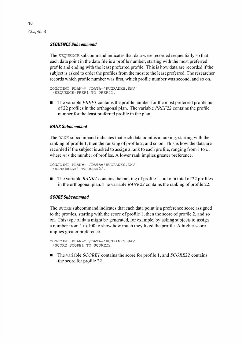
SEQUENCE Subcommand

The SEQUENCE subcommand indicates that data were recorded sequentially so that

each data point in the data file is a profile number, starting with the most preferredprofile and ending with the least preferred profile. This is how data are recorded if the

subject is asked to order the profiles from the most to the least preferred. The researcher

records which profile number was first, which profile number was second, and so on.

CONJOINT PLAN=* /DATA='RUGRANKS.SAV'/SEQUENCE=PREF1 TO PREF22.

The variable PREF1 contains the profile number for the most preferred profile out

of 22 profiles in the orthogonal plan. The variable PREF22 contains the profile

number for the least preferred profile in the plan.

RANK Subcommand

The RANK subcommand indicates that each data point is a ranking, starting with the

ranking of profile 1, then the ranking of profile 2, and so on. This is how the data are

recorded if the subject is asked to assign a rank to each profile, ranging from 1 to n,

where n is the number of profiles. A lower rank implies greater preference.

CONJOINT PLAN=* /DATA='RUGRANKS.SAV'/RANK=RANK1 TO RANK22.

The variable RANK1 contains the ranking of profile 1, out of a total of 22 profilesin the orthogonal plan. The variable RANK22 contains the ranking of profile 22.

SCORE Subcommand

The SCORE subcommand indicates that each data point is a preference score assigned

to the profiles, starting with the score of profile 1, then the score of profile 2, and so

on. This type of data might be generated, for example, by asking subjects to assign

a number from 1 to 100 to show how much they liked the profile. A higher score

implies greater preference.

CONJOINT PLAN=* /DATA='RUGRANKS.SAV'/SCORE=SCORE1 TO SCORE22.

The variable SCORE1 contains the score for profile 1, and SCORE22 contains

the score for profile 22.


25/63

17


Optional Subcommands

TheCONJOINT

command offers a number of optional subcommands that provideadditional control and functionality beyond what is required.

SUBJECT Subcommand

The SUBJECT subcommand allows you to specify a variable from the data file to

be used as an identifier for the subjects. If you do not specify a subject variable,

the CONJOINT command assumes that all of the cases in the data file come from

one subject. The following example specifies that the variable ID, from the file

rugranks.sav, is to be used as a subject identifier.

CONJOINT PLAN=* /DATA='RUGRANKS.SAV'/SCORE=SCORE1 TO SCORE22 /SUBJECT=ID.

FACTORS Subcommand

The FACTORS subcommand allows you to specify the model describing the expected

relationship between factors and the rankings or scores. If you do not specify a model

for a factor, CONJOINT assumes a discrete model. You can specify one of four models

DISCRETE. TheDISCRETE

model indicates that the factor levels are categorical andthat no assumption is made about the relationship between the factor and the scores or

ranks. This is the default.

LINEAR. The LINEAR model indicates an expected linear relationship between the

factor and the scores or ranks. You can specify the expected direction of the linear

relationship with the keywords MORE and LESS. MORE indicates that higher levels of a

factor are expected to be preferred, while LESS indicates that lower levels of a factor

are expected to be preferred. Specifying MORE orLESS will notaffect estimates of

utilities. They are used simply to identify subjects whose estimates do not match

the expected direction.

IDEAL. The IDEAL model indicates an expected quadratic relationship between the

scores or ranks and the factor. It is assumed that there is an ideal level for the factor,

and distance from this ideal point (in either direction) is associated with decreasing

preference. Factors described with this model should have at least three levels.


26/63

18

Chapter 4

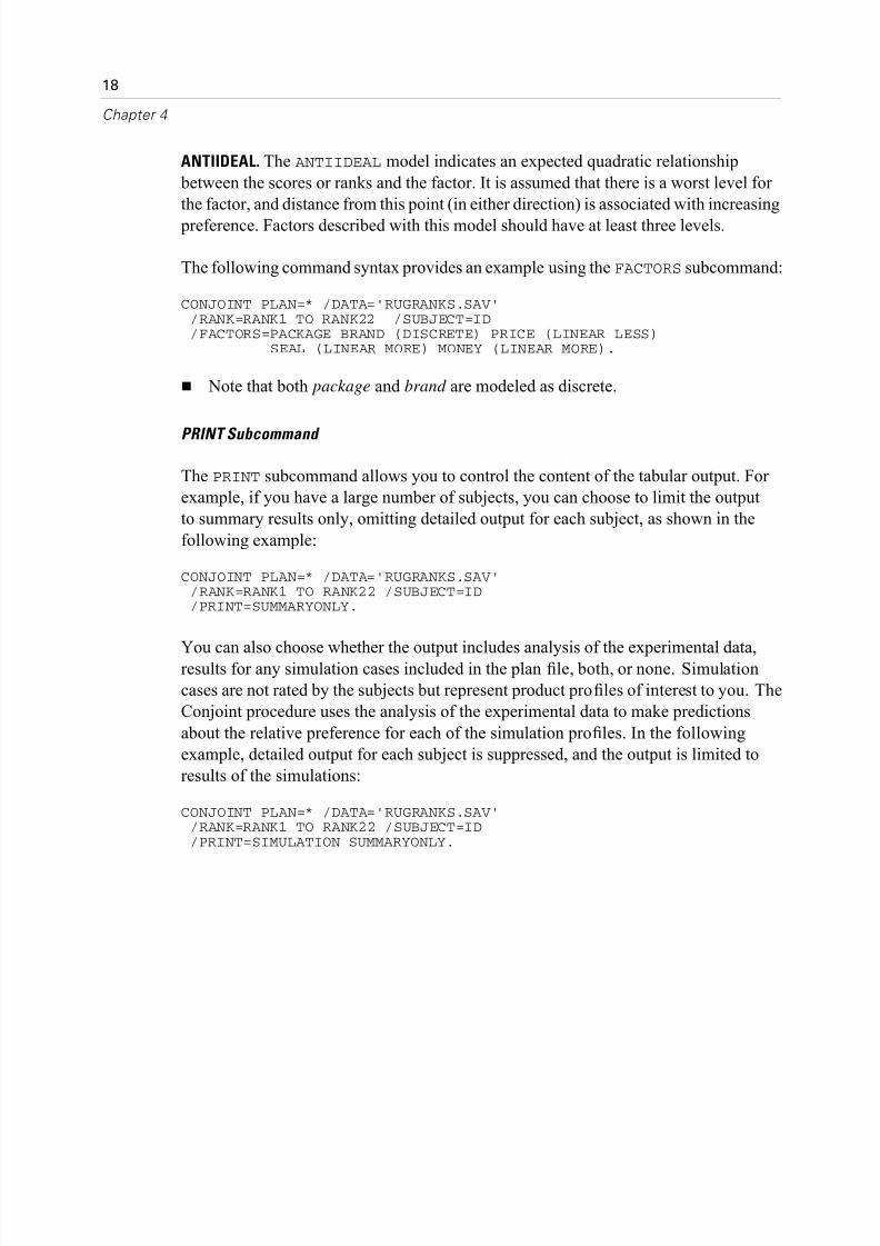
ANTIIDEAL. The ANTIIDEAL model indicates an expected quadratic relationship

between the scores or ranks and the factor. It is assumed that there is a worst level for

the factor, and distance from this point (in either direction) is associated with increasing

preference. Factors described with this model should have at least three levels.

The following command syntax provides an example using the FACTORS subcommand

CONJOINT PLAN=* /DATA='RUGRANKS.SAV'/RANK=RANK1 TO RANK22 /SUBJECT=ID/FACTORS=PACKAGE BRAND (DISCRETE) PRICE (LINEAR LESS)

SEAL (LINEAR MORE) MONEY (LINEAR MORE).

Note that both package and brandare modeled as discrete.

PRINT Subcommand

The PRINT subcommand allows you to control the content of the tabular output. For

example, if you have a large number of subjects, you can choose to limit the output

to summary results only, omitting detailed output for each subject, as shown in the

following example:

CONJOINT PLAN=* /DATA='RUGRANKS.SAV'/RANK=RANK1 TO RANK22 /SUBJECT=ID/PRINT=SUMMARYONLY.

You can also choose whether the output includes analysis of the experimental data,results for any simulation cases included in the plan file, both, or none. Simulation

cases are not rated by the subjects but represent product profiles of interest to you. The

Conjoint procedure uses the analysis of the experimental data to make predictions

about the relative preference for each of the simulation profiles. In the following

example, detailed output for each subject is suppressed, and the output is limited to

results of the simulations:

CONJOINT PLAN=* /DATA='RUGRANKS.SAV'/RANK=RANK1 TO RANK22 /SUBJECT=ID/PRINT=SIMULATION SUMMARYONLY.


27/63

19


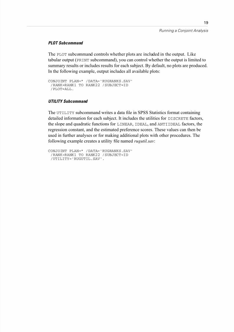
PLOT Subcommand

The PLOT subcommand controls whether plots are included in the output. Like

tabular output (PRINT subcommand), you can control whether the output is limited to

summary results or includes results for each subject. By default, no plots are produced

In the following example, output includes all available plots:

CONJOINT PLAN=* /DATA='RUGRANKS.SAV'/RANK=RANK1 TO RANK22 /SUBJECT=ID/PLOT=ALL.

UTILITY Subcommand

The UTILITY subcommand writes a data file in SPSS Statistics format containing

detailed information for each subject. It includes the utilities for DISCRETE factors,

the slope and quadratic functions for LINEAR, IDEAL, and ANTIIDEAL factors, the

regression constant, and the estimated preference scores. These values can then be

used in further analyses or for making additional plots with other procedures. The

following example creates a utility file named rugutil.sav:

CONJOINT PLAN=* /DATA='RUGRANKS.SAV'/RANK=RANK1 TO RANK22 /SUBJECT=ID/UTILITY='RUGUTIL.SAV'.


28/63

Part II:Examples


29/63

Chapte5Using Conjoint Analysis to ModelCarpet-Cleaner Preference

In a popular example of conjoint analysis (Green and Wind, 1973), a company

interested in marketing a new carpet cleaner wants to examine the influence of

five factors on consumer preferencepackage design, brand name, price, a GoodHousekeeping seal, and a money-back guarantee. There are three factor levels for

package design, each one differing in the location of the applicator brush; three brand

names (K2R, Glory, and Bissell); three price levels; and two levels (either no or yes)

for each of the last two factors. The following table displays the variables used in the

carpet-cleaner study, with their variable labels and values.

Table 5-1Variables in the carpet-cleaner study

Variable name Variable label Value label

package package design A*, B*, C*

brand brand name K2R, Glory, Bissellprice price $1.19, $1.39, $1.59

seal Good Housekeeping seal no, yes

money money-back guarantee no, yes

There could be other factors and factor levels that characterize carpet cleaners, but

these are the only ones of interest to management. This is an important point in conjoin

analysis. You want to choose only those factors (independent variables) that you

think most influence the subjects preference (the dependent variable). Using conjoint

analysis, you will develop a model for customer preference based on these five factors

This example makes use of the information in the following data files:carpet_prefs.sav contains the data collected from the subjects, carpet_plan.sav

contains the product profiles being surveyed, and conjoint.sps contains the command

21


30/63

22

Chapter 5

syntax necessary to run the analysis. For more information, see Sample Files in

Appendix A on p. 38.


The first step in a conjoint analysis is to create the combinations of factor levels that are

presented as product profiles to the subjects. Since even a small number of factors and

a few levels for each factor will lead to an unmanageable number of potential product

profiles, you need to generate a representative subset known as an orthogonal array.

The Generate Orthogonal Design procedure creates an orthogonal arrayalso

referred to as an orthogonal designand stores the information in a data file. Unlike

most procedures, an active dataset is not required before running the Generate

Orthogonal Design procedure. If you do not have an active dataset, you have theoption of creating one, generating variable names, variable labels, and value labels

from the options that you select in the dialog boxes. If you already have an active

dataset, you can either replace it or save the orthogonal design as a separate data file.

To create an orthogonal design:



Generate...


31/63

23

Using Conjoint Analysis to Model Carpet-Cleaner Preference

Figure 5-1Generate Orthogonal Design dialog box

E Enterpackage in the Factor Name text box, and enter package design in the Factor

Label text box.

E ClickAdd.

This creates an item labeled package package design (?). Select this item.

E ClickDefine Values.


32/63

24

Chapter 5

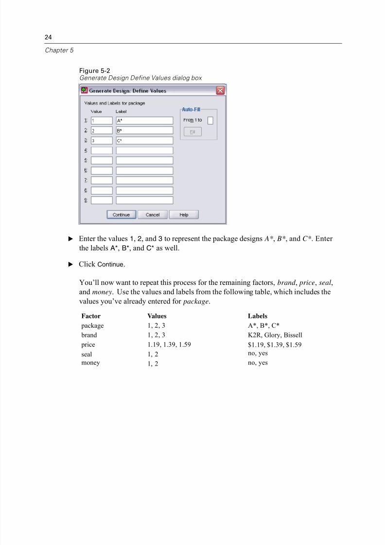
Figure 5-2Generate Design Define Values dialog box

E Enter the values 1, 2, and 3 to represent the package designs A*, B*, and C*. Enter

the labels A*, B*, and C* as well.

E ClickContinue.

Youll now want to repeat this process for the remaining factors, brand, price, seal,and money. Use the values and labels from the following table, which includes the

values youve already entered for package.

Factor Values Labels

package 1, 2, 3 A*, B*, C*

brand 1, 2, 3 K2R, Glory, Bissell

price 1.19, 1.39, 1.59 $1.19, $1.39, $1.59

seal 1, 2 no, yes

money 1, 2 no, yes


33/63

25


Once you have completed the factor specifications:

E In the Data File group, leave the default ofCreate a new dataset and enter a dataset

name. The generated design will be saved to a new dataset, in the current session,with the specified name.

E Select Reset random number seed to and enter the value 2000000.

Generating an orthogonal design requires a set of random numbers. If you want to

duplicate a designin this case, the design used for the present case studyyou need

to set the seed value before you generate the design and reset it to the same value each

subsequent time you generate the design. The design used for this case study was

generated with a seed value of 2000000.

E ClickOptions.

Figure 5-3Generate Orthogonal Design Options dialog box

E In the Minimum number of cases to generate text box, type 18.

By default, the minimum number of cases necessary for an orthogonal array is

generated. The procedure determines the number of cases that need to be administered

to allow estimation of the utilities. You can also specify a minimum number of cases to

generate, as youve done here. You might want to do this because the default number

of minimum cases is too small to be useful or because you have experimental design

considerations that require a certain minimum number of cases.

E Select Number of holdout cases and type 4.

Holdout cases are judged by the subjects but are not used by the conjoint analysis to

estimate utilities. They are used as a check on the validity of the estimated utilities.

The holdout cases are generated from another random plan, not the experimental

orthogonal plan.


34/63

26

Chapter 5

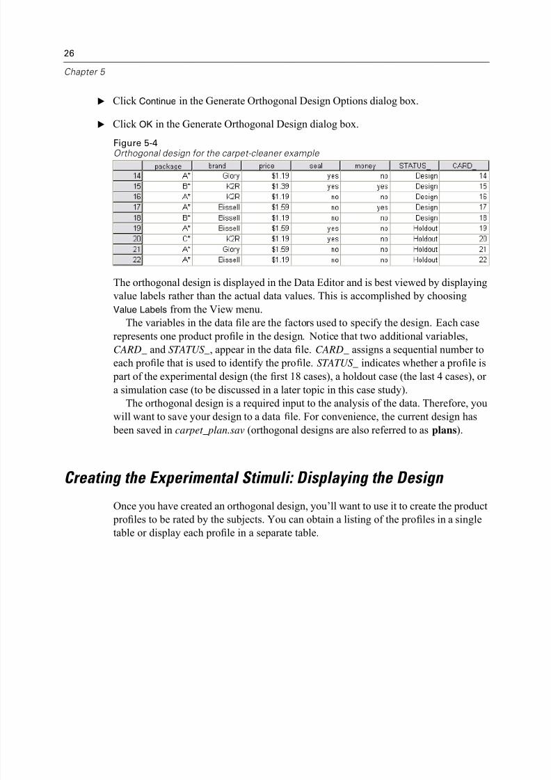
E ClickContinue in the Generate Orthogonal Design Options dialog box.

E ClickOK in the Generate Orthogonal Design dialog box.

Figure 5-4Orthogonal design for the carpet-cleaner example

The orthogonal design is displayed in the Data Editor and is best viewed by displaying

value labels rather than the actual data values. This is accomplished by choosing

Value Labels from the View menu.

The variables in the data file are the factors used to specify the design. Each case

represents one product profile in the design. Notice that two additional variables,

CARD_ and STATUS_, appear in the data file. CARD_ assigns a sequential number to

each profile that is used to identify the profile. STATUS_ indicates whether a profile is

part of the experimental design (the first 18 cases), a holdout case (the last 4 cases), or

a simulation case (to be discussed in a later topic in this case study).

The orthogonal design is a required input to the analysis of the data. Therefore, youwill want to save your design to a data file. For convenience, the current design has

been saved in carpet_plan.sav (orthogonal designs are also referred to as plans).

Creating the Experimental Stimuli: Displaying the Design

Once you have created an orthogonal design, youll want to use it to create the product

profiles to be rated by the subjects. You can obtain a listing of the profiles in a single

table or display each profile in a separate table.


35/63

27


To display an orthogonal design:



Display...

Figure 5-5Display Design dialog box

E Select package, brand, price, seal, and money for the factors.

The information contained in the variables STATUS_ and CARD_ is automatically

included in the output, so they dont need to be selected.

E Select Listing for experimenter in the Format group. This results in displaying the entire

orthogonal design in a single table.

E ClickOK.


36/63

28

Chapter 5

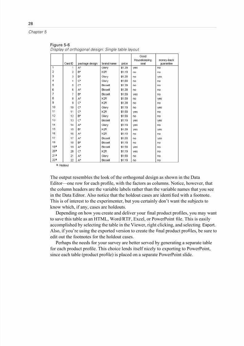
Figure 5-6Display of orthogonal design: Single table layout

The output resembles the look of the orthogonal design as shown in the Data

Editorone row for each profile, with the factors as columns. Notice, however, that

the column headers are the variable labels rather than the variable names that you see

in the Data Editor. Also notice that the holdout cases are identified with a footnote.

This is of interest to the experimenter, but you certainly dont want the subjects to

know which, if any, cases are holdouts.

Depending on how you create and deliver yourfinal product profiles, you may wan

to save this table as an HTML, Word/RTF, Excel, or PowerPoint file. This is easily

accomplished by selecting the table in the Viewer, right clicking, and selecting Export.

Also, if youre using the exported version to create the final product profiles, be sure to

edit out the footnotes for the holdout cases.

Perhaps the needs for your survey are better served by generating a separate tablefor each product profile. This choice lends itself nicely to exporting to PowerPoint,

since each table (product profile) is placed on a separate PowerPoint slide.


37/63

29


To display each profile in a separate table:

E Click the Dialog Recall button and select Display Design.

E Deselect Listing for experimenter and select Profiles for subjects.

E ClickOK.

Figure 5-7Display of orthogonal design: Multitable layout

The information for each product profile is displayed in a separate table. In addition,

holdout cases are indistinguishable from the rest of the cases, so there is no issue of

removing identifiers for holdouts as with the single table layout.

Running the Analysis

Youve generated an orthogonal design and learned how to display the associated

product profiles. Youre now ready to learn how to run a conjoint analysis.


38/63

30

Chapter 5

Figure 5-8Preference data for the carpet-cleaner example

The preference data collected from the subjects is stored in carpet_prefs.sav. The data

consist of responses from 10 subjects, each identified by a unique value of the variableID. Subjects were asked to rank the 22 product profiles from the most to the least

preferred. The variables PREF1 through PREF22 contain the IDs of the associated

product profiles, that is, the card IDs from carpet_plan.sav. Subject 1, for example,

liked profile 13 most of all, so PREF1 has the value 13.

Analysis of the data is a task that requires the use of command syntaxspecifically

the CONJOINT command. The necessary command syntax has been provided in the

file conjoint.sps.

CONJOINT PLAN='file specification'/DATA='file specification'

/SEQUENCE=PREF1 TO PREF22/SUBJECT=ID/FACTORS=PACKAGE BRAND (DISCRETE)

PRICE (LINEAR LESS)SEAL (LINEAR MORE) MONEY (LINEAR MORE)

/PRINT=SUMMARYONLY.

The PLAN subcommand specifies the file containing the orthogonal designin

this example, carpet_plan.sav.

The DATA subcommand specifies the file containing the preference datain this

example, carpet_prefs.sav . If you choose the preference data as the active dataset,

you can replace the file specification with an asterisk (*), without the quotation

marks.

The SEQUENCE subcommand specifies that each data point in the preference data

is a profile number, starting with the most-preferred profile and ending with the

least-preferred profile.


39/63

31


The SUBJECT subcommand specifies that the variable ID identifies the subjects.

The FACTORS subcommand specifies a model describing the expected relationship

between the preference data and the factor levels. The specifi

ed factors refer tovariables defined in the plan file named on the PLAN subcommand.

The keyword DISCRETE is used when the factor levels are categorical and no

assumption is made about the relationship between the levels and the data. This

is the case for the factors package and brandthat represent package design and

brand name, respectively. DISCRETE is assumed if a factor is not labeled with

one of the four alternatives (DISCRETE, LINEAR, IDEAL, ANTIIDEAL) or is not

included on the FACTORS subcommand.

The keyword LINEAR, used for the remaining factors, indicates that the data are

expected to be linearly related to the factor. For example, preference is usually

expected to be linearly related to price. You can also specify quadratic models (notused in this example) with the keywords IDEAL and ANTIIDEAL.

The keywords MORE and LESS, following LINEAR, indicate an expected direction

for the relationship. Since we expect higher preference for lower prices, the

keyword LESS is used forprice. However, we expect higher preference for either

a Good Housekeeping seal of approval or a money-back guarantee, so the keyword

MORE is used forseal and money (recall that the levels for both of these factors

were set to 1 forno and 2 foryes).

Specifying MORE orLESS does not change the signs of the coefficients or affect

estimates of the utilities. These keywords are used simply to identify subjects

whose estimates do not match the expected direction. Similarly, choosing IDEALinstead ofANTIIDEAL, or vice versa, does not affect coefficients or utilities.

The PRINT subcommand specifies that the output contains information for the

group of subjects only as a whole (SUMMARYONLY keyword). Information for

each subject, separately, is suppressed.

Try running this command syntax. Make sure that you have included valid paths to

carpet_prefs.sav and carpet_plan.sav. For a complete description of all options, see

the CONJOINT command in the Command Syntax Reference.


40/63

32

Chapter 5

Utility ScoresFigure 5-9

Utility scores

This table shows the utility (part-worth) scores and their standard errors for each facto

level. Higher utility values indicate greater preference. As expected, there is an inverse

relationship between price and utility, with higher prices corresponding to lower utility

(larger negative values mean lower utility). The presence of a seal of approval or

money-back guarantee corresponds to a higher utility, as anticipated.

Since the utilities are all expressed in a common unit, they can be added together

to give the total utility of any combination. For example, the total utility of a

cleaner with package design B*, brand K2R, price $1.19, and no seal of approval ormoney-back guarantee is:

utility(package B*) + utility(K2R) + utility($1.19)

+ utility(no seal) + utility(no money-back) + constant

or

1.867 + 0.367 + (6.595) + 2.000 + 1.250 + 12.870 = 11.759

If the cleaner had package design C*, brand Bissell, price $1.59, a seal of approval,

and a money-back guarantee, the total utility would be:

0.367 + (0.017) + (8.811) + 4.000 + 2.500 + 12.870 = 10.909


41/63

33


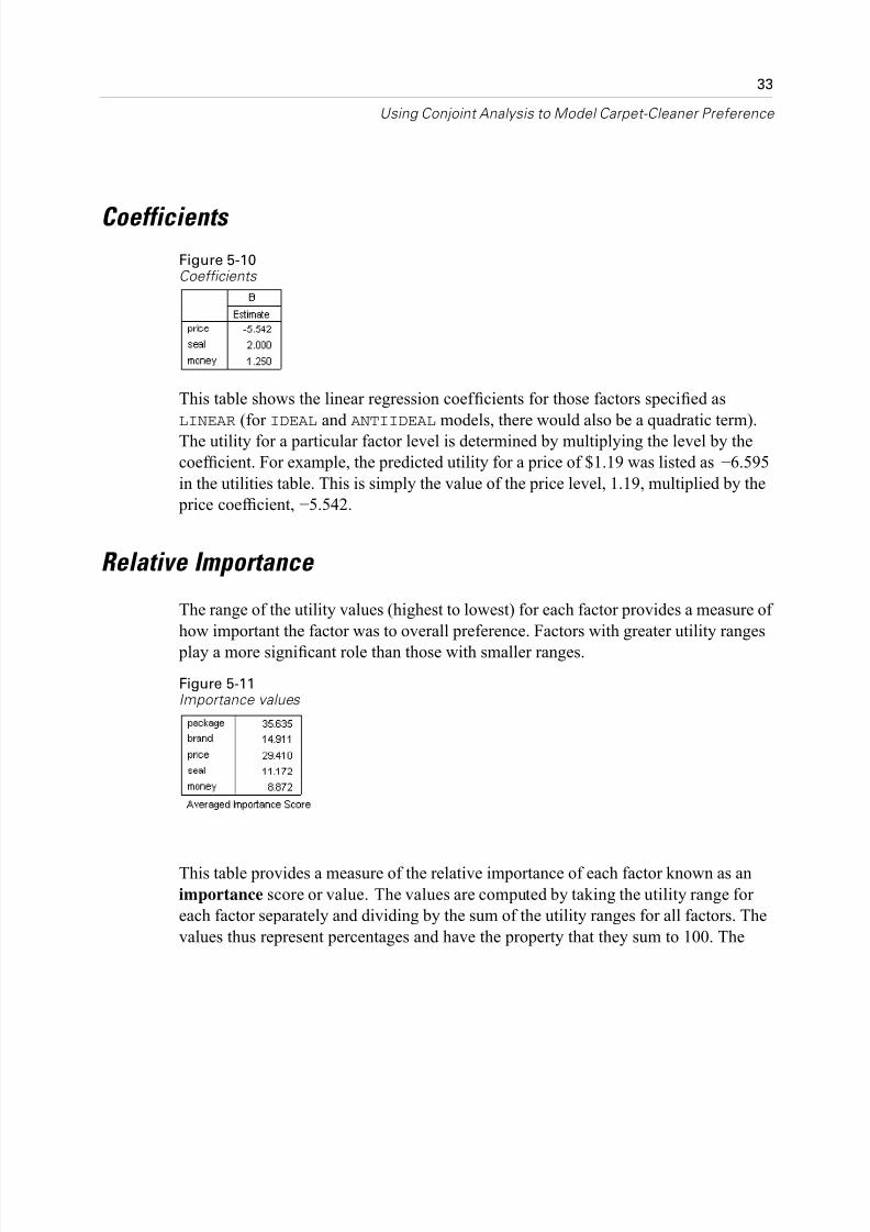
CoefficientsFigure 5-10Coefficients

This table shows the linear regression coefficients for those factors specified as

LINEAR (forIDEAL and ANTIIDEAL models, there would also be a quadratic term).

The utility for a particular factor level is determined by multiplying the level by the

coefficient. For example, the predicted utility for a price of $1.19 was listed as 6.595

in the utilities table. This is simply the value of the price level, 1.19, multiplied by the

price coefficient, 5.542.

Relative Importance

The range of the utility values (highest to lowest) for each factor provides a measure o

how important the factor was to overall preference. Factors with greater utility ranges

play a more significant role than those with smaller ranges.

Figure 5-11Importance values

This table provides a measure of the relative importance of each factor known as an

importance score or value. The values are computed by taking the utility range for

each factor separately and dividing by the sum of the utility ranges for all factors. The

values thus represent percentages and have the property that they sum to 100. The


42/63

34

Chapter 5

calculations, it should be noted, are done separately for each subject, and the results

are then averaged over all of the subjects.

Note that while overall or summary utilities and regression coefficients from

orthogonal designs are the same with or without a SUBJECT subcommand, importance

will generally differ. For summary results without a SUBJECT subcommand, the

importances can be computed directly from the summary utilities, just as one can

do with individual subjects. However, when a SUBJECT subcommand is used, the

importances for the individual subjects are averaged, and these averaged importances

will not in general match those computed using the summary utilities.

The results show that package design has the most influence on overall preference.

This means that there is a large difference in preference between product profiles

containing the most desired packaging and those containing the least desired packaging

The results also show that a money-back guarantee plays the least important role in

determining overall preference. Price plays a significant role but not as significant aspackage design. Perhaps this is because the range of prices is not that large.

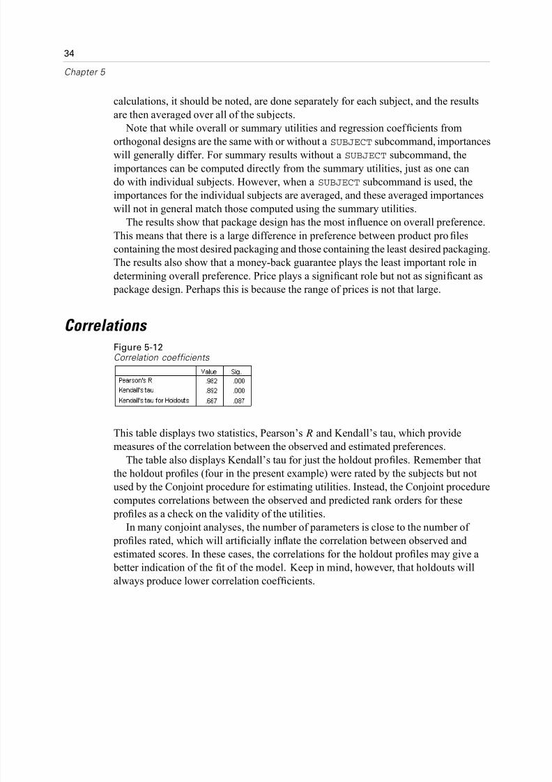
CorrelationsFigure 5-12Correlation coefficients

This table displays two statistics, Pearsons R and Kendalls tau, which provide

measures of the correlation between the observed and estimated preferences.

The table also displays Kendalls tau for just the holdout profiles. Remember that

the holdout profiles (four in the present example) were rated by the subjects but not

used by the Conjoint procedure for estimating utilities. Instead, the Conjoint procedure

computes correlations between the observed and predicted rank orders for these

profiles as a check on the validity of the utilities.

In many conjoint analyses, the number of parameters is close to the number of

profi

les rated, which will artifi

cially infl

ate the correlation between observed andestimated scores. In these cases, the correlations for the holdout profiles may give a

better indication of the fit of the model. Keep in mind, however, that holdouts will

always produce lower correlation coefficients.


43/63

35


Reversals

When specifying LINEAR models forprice, seal, and money, we chose an expected

direction (LESS orMORE) for the linear relationship between the value of the variable

and the preference for that value. The Conjoint procedure keeps track of the number

of subjects whose preference showed the opposite of the expected relationshipfor

example, a greater preference for higher prices, or a lower preference for a money-back

guarantee. These cases are referred to as reversals.

Figure 5-13Number of reversals by factor and subject

This table displays the number of reversals for each factor and for each subject. For

example, three subjects showed a reversal for price. That is, they preferred product

profiles with higher prices.

Running Simulations

The real power of conjoint analysis is the ability to predict preference for product

profiles that werent rated by the subjects. These are referred to as simulation cases.

Simulation cases are included as part of the plan, along with the profiles from the

orthogonal design and any holdout profiles.

The simplest way to enter simulation cases is from the Data Editor, using the valuelabels created when you generated the experimental design.


44/63

36

Chapter 5

To enter a simulation case in the plan file:

E On a new row in the Data Editor window, select a cell and select the desired value from

the list (value labels can be displayed by choosing Value Labels from the View menu).Repeat for all of the variables (factors).

E Select Simulation for the value of the STATUS_ variable.

E Enter an integer value, to be used as an identifier, for the CARD_ variable. Simulation

cases should be numbered separately from the other cases.

Figure 5-14Carpet-cleaner data including simulation cases

The figure shows a part of the plan file for the carpet-cleaner study, with two simulation

cases added. For convenience, these have been included in carpet_plan.sav.

The analysis of the simulation cases is accomplished with the same command

syntax used earlier, that is, the syntax in thefi

leconjoint.sps

. In fact, if you ran thesyntax described earlier, you would have noticed that the output also includes results

for the simulation cases, since they are included in carpet_plan.sav.

You can choose to run simulations along with your initial analysisas done

hereor run simulations at any later point simply by including simulation cases in

your plan file and rerunning CONJOINT. For more information, see the CONJOINT

command in the Command Syntax Reference.


45/63

37


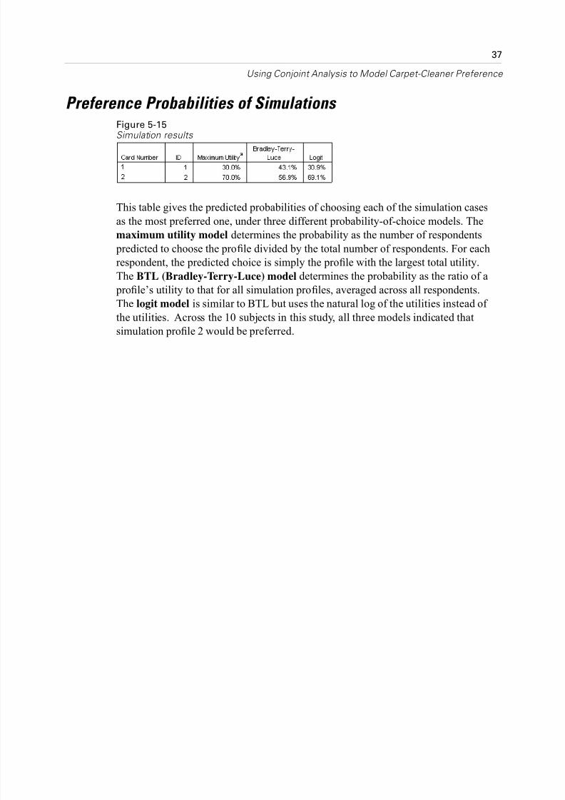
Preference Probabilities of SimulationsFigure 5-15

Simulation results

This table gives the predicted probabilities of choosing each of the simulation cases

as the most preferred one, under three different probability-of-choice models. The

maximum utility model determines the probability as the number of respondents

predicted to choose the profile divided by the total number of respondents. For each

respondent, the predicted choice is simply the profile with the largest total utility.

The BTL (Bradley-Terry-Luce) model determines the probability as the ratio of aprofiles utility to that for all simulation profiles, averaged across all respondents.

The logit model is similar to BTL but uses the natural log of the utilities instead of

the utilities. Across the 10 subjects in this study, all three models indicated that

simulation profile 2 would be preferred.


46/63

AppendixASample Files

The sample files installed with the product can be found in the Samples subdirectory o

the installation directory. There is a separate folder within the Samples subdirectory for

each of the following languages: English, French, German, Italian, Japanese, Korean,

Polish, Russian, Simplified Chinese, Spanish, and Traditional Chinese.

Not all sample files are available in all languages. If a sample file is not available in a

language, that language folder contains an English version of the sample file.

Descriptions

Following are brief descriptions of the sample files used in various examples

throughout the documentation.

accidents.sav. This is a hypothetical data file that concerns an insurance company

that is studying age and gender risk factors for automobile accidents in a given

region. Each case corresponds to a cross-classification of age category and gender

adl.sav. This is a hypothetical data file that concerns efforts to determine the

benefits of a proposed type of therapy for stroke patients. Physicians randomly

assigned female stroke patients to one of two groups. The first received the

standard physical therapy, and the second received an additional emotional

therapy. Three months following the treatments, each patients abilities to perform

common activities of daily life were scored as ordinal variables.

advert.sav. This is a hypothetical data file that concerns a retailers efforts to

examine the relationship between money spent on advertising and the resulting

sales. To this end, they have collected past sales figures and the associated

advertising costs..

38


47/63

39

Sample Files

aflatoxin.sav. This is a hypothetical data file that concerns the testing of corn crops

for aflatoxin, a poison whose concentration varies widely between and within crop

yields. A grain processor has received 16 samples from each of 8 crop yields and

measured the alfatoxin levels in parts per billion (PPB).

aflatoxin20.sav. This data file contains the aflatoxin measurements from each of the

16 samples from yields 4 and 8 from the aflatoxin.sav data file.

anorectic.sav. While working toward a standardized symptomatology of

anorectic/bulimic behavior, researchers (Van der Ham, Meulman, Van Strien, and

Van Engeland, 1997) made a study of 55 adolescents with known eating disorders

Each patient was seen four times over four years, for a total of 220 observations.

At each observation, the patients were scored for each of 16 symptoms. Symptom

scores are missing for patient 71 at time 2, patient 76 at time 2, and patient 47 at

time 3, leaving 217 valid observations.

autoaccidents.sav. This is a hypothetical data file that concerns the efforts of an

insurance analyst to model the number of automobile accidents per driver while

also accounting for driver age and gender. Each case represents a separate driver

and records the drivers gender, age in years, and number of automobile accidents

in the last five years.

band.sav. This data file contains hypothetical weekly sales figures of music CDs

for a band. Data for three possible predictor variables are also included.

bankloan.sav. This is a hypothetical data file that concerns a banks efforts to reduce

the rate of loan defaults. The file contains financial and demographic information

on 850 past and prospective customers. Thefi

rst 700 cases are customers whowere previously given loans. The last 150 cases are prospective customers that

the bank needs to classify as good or bad credit risks.

bankloan_binning.sav. This is a hypothetical data file containing financial and

demographic information on 5,000 past customers.

behavior.sav. In a classic example (Price and Bouffard, 1974), 52 students were

asked to rate the combinations of 15 situations and 15 behaviors on a 10-point

scale ranging from 0=extremely appropriate to 9=extremely inappropriate.

Averaged over individuals, the values are taken as dissimilarities.

behavior_ini.sav. This data file contains an initial configuration for a

two-dimensional solution forbehavior.sav.


48/63

40

Appendix A

brakes.sav. This is a hypothetical data file that concerns quality control at a factory

that produces disc brakes for high-performance automobiles. The data file contain

diameter measurements of 16 discs from each of 8 production machines. The

target diameter for the brakes is 322 millimeters.

breakfast.sav. In a classic study (Green and Rao, 1972), 21 Wharton School MBA

students and their spouses were asked to rank 15 breakfast items in order of

preference with 1=most preferred to 15=least preferred. Their preferences

were recorded under six different scenarios, from Overall preference to Snack,

with beverage only.

breakfast-overall.sav. This data file contains the breakfast item preferences for the

first scenario, Overall preference, only.

broadband_1.sav. This is a hypothetical data file containing the number of

subscribers, by region, to a national broadband service. The datafi

le containsmonthly subscriber numbers for 85 regions over a four-year period.

broadband_2.sav. This data file is identical to broadband_1.sav but contains data

for three additional months.

car_insurance_claims.sav. A dataset presented and analyzed elsewhere (McCullagh

and Nelder, 1989) concerns damage claims for cars. The average claim amount

can be modeled as having a gamma distribution, using an inverse link function

to relate the mean of the dependent variable to a linear combination of the

policyholder age, vehicle type, and vehicle age. The number of claims filed can

be used as a scaling weight.

car_sales.sav. This data file contains hypothetical sales estimates, list prices,and physical specifications for various makes and models of vehicles. The list

prices and physical specifications were obtained alternately from edmunds.com

and manufacturer sites.

carpet.sav. In a popular example (Green and Wind, 1973), a company interested in

marketing a new carpet cleaner wants to examine the influence offive factors on

consumer preferencepackage design, brand name, price, a Good Housekeeping

seal, and a money-back guarantee. There are three factor levels for package

design, each one differing in the location of the applicator brush; three brand

names (K2R, Glory, and Bissell); three price levels; and two levels (either no or

yes) for each of the last two factors. Ten consumers rank 22 profiles defined bythese factors. The variable Preference contains the rank of the average rankings

for each profile. Low rankings correspond to high preference. This variable

reflects an overall measure of preference for each profile.


49/63

41

Sample Files

carpet_prefs.sav. This data file is based on the same example as described for

carpet.sav, but it contains the actual rankings collected from each of the 10

consumers. The consumers were asked to rank the 22 product profiles from the

most to the least preferred. The variables PREF1 through PREF22 contain theidentifiers of the associated profiles, as defined in carpet_plan.sav.

catalog.sav. This data file contains hypothetical monthly sales figures for three

products sold by a catalog company. Data forfive possible predictor variables

are also included.

catalog_seasfac.sav. This data file is the same as catalog.sav except for the

addition of a set of seasonal factors calculated from the Seasonal Decomposition

procedure along with the accompanying date variables.

cellular.sav. This is a hypothetical data file that concerns a cellular phone

companys efforts to reduce churn. Churn propensity scores are applied toaccounts, ranging from 0 to 100. Accounts scoring 50 or above may be looking to

change providers.

ceramics.sav. This is a hypothetical data file that concerns a manufacturers efforts

to determine whether a new premium alloy has a greater heat resistance than a

standard alloy. Each case represents a separate test of one of the alloys; the heat at

which the bearing failed is recorded.

cereal.sav. This is a hypothetical data file that concerns a poll of 880 people about

their breakfast preferences, also noting their age, gender, marital status, and

whether or not they have an active lifestyle (based on whether they exercise at

least twice a week). Each case represents a separate respondent. clothing_defects.sav. This is a hypothetical data file that concerns the quality

control process at a clothing factory. From each lot produced at the factory, the

inspectors take a sample of clothes and count the number of clothes that are

unacceptable.

coffee.sav. This data file pertains to perceived images of six iced-coffee brands

(Kennedy, Riquier, and Sharp, 1996) . For each of 23 iced-coffee image attributes

people selected all brands that were described by the attribute. The six brands are

denoted AA, BB, CC, DD, EE, and FF to preserve confidentiality.

contacts.sav. This is a hypothetical data file that concerns the contact lists for a

group of corporate computer sales representatives. Each contact is categorizedby the department of the company in which they work and their company ranks.

Also recorded are the amount of the last sale made, the time since the last sale,

and the size of the contacts company.


50/63

42

Appendix A

creditpromo.sav. This is a hypothetical data file that concerns a department stores

efforts to evaluate the effectiveness of a recent credit card promotion. To this

end, 500 cardholders were randomly selected. Half received an ad promoting a

reduced interest rate on purchases made over the next three months. Half receiveda standard seasonal ad.

customer_dbase.sav. This is a hypothetical data file that concerns a companys

efforts to use the information in its data warehouse to make special offers to

customers who are most likely to reply. A subset of the customer base was selected

at random and given the special offers, and their responses were recorded.

customer_information.sav. A hypothetical data file containing customer mailing

information, such as name and address.

customers_model.sav. This file contains hypothetical data on individuals targeted

by a marketing campaign. These data include demographic information, asummary of purchasing history, and whether or not each individual responded to

the campaign. Each case represents a separate individual.

customers_new.sav. This file contains hypothetical data on individuals who are

potential candidates for a marketing campaign. These data include demographic

information and a summary of purchasing history for each individual. Each case

represents a separate individual.

debate.sav. This is a hypothetical data file that concerns paired responses to a

survey from attendees of a political debate before and after the debate. Each case

corresponds to a separate respondent.

debate_aggregate.sav. This is a hypothetical data file that aggregates the responsesin debate.sav. Each case corresponds to a cross-classification of preference before

and after the debate.

demo.sav. This is a hypothetical data file that concerns a purchased customer

database, for the purpose of mailing monthly offers. Whether or not the customer

responded to the offer is recorded, along with various demographic information.

demo_cs_1.sav. This is a hypothetical data file that concerns the first step of

a companys efforts to compile a database of survey information. Each case

corresponds to a different city, and the region, province, district, and city

identification are recorded.

demo_cs_2.sav. This is a hypothetical data file that concerns the second step

of a companys efforts to compile a database of survey information. Each case

corresponds to a different household unit from cities selected in the first step, and


51/63

43

Sample Files

the region, province, district, city, subdivision, and unit identification are recorded

The sampling information from the first two stages of the design is also included.

demo_cs.sav. This is a hypothetical datafi

le that contains survey informationcollected using a complex sampling design. Each case corresponds to a different

household unit, and various demographic and sampling information is recorded.

dietstudy.sav. This hypothetical data file contains the results of a study of the

Stillman diet (Rickman, Mitchell, Dingman, and Dalen, 1974). Each case

corresponds to a separate subject and records his or her pre- and post-diet weights

in pounds and triglyceride levels in mg/100 ml.

dischargedata.sav. This is a data file concerning Seasonal Patterns of Winnipeg

Hospital Use, (Menec , Roos, Nowicki, MacWilliam, Finlayson , and Black, 1999)

from the Manitoba Centre for Health Policy.

dvdplayer.sav. This is a hypothetical data file that concerns the development of anew DVD player. Using a prototype, the marketing team has collected focus

group data. Each case corresponds to a separate surveyed user and records some

demographic information about them and their responses to questions about the

prototype.

flying.sav. This data file contains the flying mileages between 10 American cities.

german_credit.sav. This data file is taken from the German credit dataset in

the Repository of Machine Learning Databases (Blake and Merz, 1998) at the

University of California, Irvine.

grocery_1month.sav. This hypothetical data file is the grocery_coupons.sav data file

with the weekly purchases rolled-up so that each case corresponds to a separate

customer. Some of the variables that changed weekly disappear as a result, and

the amount spent recorded is now the sum of the amounts spent during the four

weeks of the study.

grocery_coupons.sav. This is a hypothetical data file that contains survey data

collected by a grocery store chain interested in the purchasing habits of their

customers. Each customer is followed for four weeks, and each case corresponds

to a separate customer-week and records information about where and how the

customer shops, including how much was spent on groceries during that week.

guttman.sav. Bell (Bell, 1961) presented a table to illustrate possible social groups.

Guttman (Guttman, 1968) used a portion of this table, in which five variables

describing such things as social interaction, feelings of belonging to a group,

physical proximity of members, and formality of the relationship were crossed

with seven theoretical social groups, including crowds (for example, people at a


52/63

44

Appendix A

football game), audiences (for example, people at a theater or classroom lecture),

public (for example, newspaper or television audiences), mobs (like a crowd but

with much more intense interaction), primary groups (intimate), secondary groups

(voluntary), and the modern community (loose confederation resulting from closephysical proximity and a need for specialized services).

healthplans.sav. This is a hypothetical data file that concerns an insurance groups

efforts to evaluate four different health care plans for small employers. Twelve

employers are recruited to rank the plans by how much they would prefer to

offer them to their employees. Each case corresponds to a separate employer

and records the reactions to each plan.

health_funding.sav. This is a hypothetical data file that contains data on health care

funding (amount per 100 population), disease rates (rate per 10,000 population),

and visits to health care providers (rate per 10,000 population). Each case

represents a different city.

hivassay.sav. This is a hypothetical data file that concerns the efforts of a

pharmaceutical lab to develop a rapid assay for detecting HIV infection. The

results of the assay are eight deepening shades of red, with deeper shades indicating

greater likelihood of infection. A laboratory trial was conducted on 2,000 blood

samples, half of which were infected with HIV and half of which were clean.

hourlywagedata.sav. This is a hypothetical data file that concerns the hourly wages

of nurses from office and hospital positions and with varying levels of experience.

insure.sav. This is a hypothetical data file that concerns an insurance company that

is studying the risk factors that indicate whether a client will have to make a claimon a 10-year term life insurance contract. Each case in the data file represents a

pair of contracts, one of which recorded a claim and the other didnt, matched

on age and gender.

judges.sav. This is a hypothetical data file that concerns the scores given by trained

judges (plus one enthusiast) to 300 gymnastics performances. Each row represents

a separate performance; the judges viewed the same performances.

kinship_dat.sav. Rosenberg and Kim (Rosenberg and Kim, 1975) set out to

analyze 15 kinship terms (aunt, brother, cousin, daughter, father, granddaughter,

grandfather, grandmother, grandson, mother, nephew, niece, sister, son, uncle).

They asked four groups of college students (two female, two male) to sort theseterms on the basis of similarities. Two groups (one female, one male) were asked

to sort twice, with the second sorting based on a different criterion from the first

sort. Thus, a total of six sources were obtained. Each source corresponds to a


53/63

45

Sample Files

proximity matrix, whose cells are equal to the number of people in a source

minus the number of times the objects were partitioned together in that source.

kinship_ini.sav. This datafi

le contains an initial confi

guration for athree-dimensional solution forkinship_dat.sav.

kinship_var.sav. This data file contains independent variables gender, gener(ation)

and degree (of separation) that can be used to interpret the dimensions of a solution

forkinship_dat.sav. Specifically, they can be used to restrict the space of the

solution to a linear combination of these variables.

mailresponse.sav. This is a hypothetical data file that concerns the efforts of a

clothing manufacturer to determine whether using first class postage for direct

mailings results in faster responses than bulk mail. Order-takers record how many

weeks after the mailing each order is taken.

marketvalues.sav. This data file concerns home sales in a new housing developmenin Algonquin, Ill., during the years from 19992000. These sales are a matter

of public record.

mutualfund.sav. This data file concerns stock market information for various tech

stocks listed on the S&P 500. Each case corresponds to a separate company.

nhis2000_subset.sav. The National Health Interview Survey (NHIS) is a large,

population-based survey of the U.S. civilian population. Interviews are

carried out face-to-face in a nationally representative sample of households.

Demographic information and observations about health behaviors and status

are obtained for members of each household. This data file contains a subset

of information from the 2000 survey. National Center for Health Statistics.National Health Interview Survey, 2000. Public-use data file and documentation.

ftp://ftp.cdc.gov/pub/Health_Statistics/NCHS/Datasets/NHIS/2000/. Accessed

2003.

ozone.sav. The data include 330 observations on six meteorological variables for

predicting ozone concentration from the remaining variables. Previous researcher

(Breiman and Friedman, 1985), (Hastie and Tibshirani, 1990), among others found

nonlinearities among these variables, which hinder standard regression approaches

pain_medication.sav. This hypothetical data file contains the results of a clinical

trial for anti-inflammatory medication for treating chronic arthritic pain. Of

particular interest is the time it takes for the drug to take effect and how itcompares to an existing medication.


54/63

46

Appendix A

patient_los.sav. This hypothetical data file contains the treatment records of

patients who were admitted to the hospital for suspected myocardial infarction

(MI, or heart attack). Each case corresponds to a separate patient and records

many variables related to their hospital stay.

patlos_sample.sav. This hypothetical data file contains the treatment records of a

sample of patients who received thrombolytics during treatment for myocardial

infarction (MI, or heart attack). Each case corresponds to a separate patient and

records many variables related to their hospital stay.

polishing.sav. This is the Nambeware Polishing Times data file from the Data and

Story Library. It concerns the efforts of a metal tableware manufacturer (Nambe

Mills, Santa Fe, N. M.) to plan its production schedule. Each case represents a

different item in the product line. The diameter, polishing time, price, and product

type are recorded for each item.

poll_cs.sav. This is a hypothetical data file that concerns pollsters efforts to

determine the level of public support for a bill before the legislature. The cases

correspond to registered voters. Each case records the county, township, and

neighborhood in which the voter lives.

poll_cs_sample.sav. This hypothetical data file contains a sample of the voters

listed in poll_cs.sav. The sample was taken according to the design specified in

the poll.csplan plan file, and this data file records the inclusion probabilities and

sample weights. Note, however, that because the sampling plan makes use of

a probability-proportional-to-size (PPS) method, there is also a file containing

the joint selection probabilities (poll_jointprob.sav). The additional variables

corresponding to voter demographics and their opinion on the proposed bill were

collected and added the data file after the sample as taken.

property_assess.sav. This is a hypothetical data file that concerns a county

assessors efforts to keep property value assessments up to date on limited

resources. The cases correspond to properties sold in the county in the past year.

Each case in the data file records the township in which the property lies, the

assessor who last visited the property, the time since that assessment, the valuation

made at that time, and the sale value of the property.

property_assess_cs.sav. This is a hypothetical data file that concerns a state

assessors efforts to keep property value assessments up to date on limited

resources. The cases correspond to properties in the state. Each case in the data

file records the county, township, and neighborhood in which the property lies, the

time since the last assessment, and the valuation made at that time.


55/63

47

Sample Files

property_assess_cs_sample.sav. This hypothetical data file contains a sample of

the properties listed in property_assess_cs.sav. The sample was taken according

to the design specified in the property_assess.csplan plan file, and this data file

records the inclusion probabilities and sample weights. The additional variableCurrent value was collected and added to the data file after the sample was taken.

recidivism.sav. This is a hypothetical data file that concerns a government law

enforcement agencys efforts to understand recidivism rates in their area of

jurisdiction. Each case corresponds to a previous offender and records their

demographic information, some details of theirfirst crime, and then the time until

their second arrest, if it occurred within two years of the first arrest.

recidivism_cs_sample.sav. This is a hypothetical data file that concerns a

government law enforcement agencys efforts to understand recidivism rates

in their area of jurisdiction. Each case corresponds to a previous offender,

released from theirfirst arrest during the month of June, 2003, and records

their demographic information, some details of theirfirst crime, and the data

of their second arrest, if it occurred by the end of June, 2006. Offenders were

selected from sampled departments according to the sampling plan specified in

recidivism_cs.csplan; because it makes use of a probability-proportional-to-size

(PPS) method, there is also a file containing the joint selection probabilities

(recidivism_cs_jointprob.sav ).

rfm_transactions.sav. A hypothetical data file containing purchase transaction

data, including date of purchase, item(s) purchased, and monetary amount of

each transaction.

salesperformance.sav. This is a hypothetical data file that concerns the evaluation

of two new sales training courses. Sixty employees, divided into three groups, all

receive standard training. In addition, group 2 gets technical training; group 3,

a hands-on tutorial. Each employee was tested at the end of the training course

and their score recorded. Each case in the data file represents a separate trainee

and records the group to which they were assigned and the score they received

on the exam.

satisf.sav. This is a hypothetical data file that concerns a satisfaction survey

conducted by a retail company at 4 store locations. 582 customers were surveyed

in all, and each case represents the responses from a single customer.

screws.sav. This data file contains information on the characteristics of screws,

bolts, nuts, and tacks (Hartigan, 1975).


56/63

48

Appendix A

shampoo_ph.sav. This is a hypothetical data file that concerns the quality control at

a factory for hair products. At regular time intervals, six separate output batches

are measured and their pH recorded. The target range is 4.55.5.

ships.sav. A dataset presented and analyzed elsewhere (McCullagh et al., 1989)

that concerns damage to cargo ships caused by waves. The incident counts can be

modeled as occurring at a Poisson rate given the ship type, construction period, and

service period. The aggregate months of service for each cell of the table formed

by the cross-classification of factors provides values for the exposure to risk.

site.sav. This is a hypothetical data file that concerns a companys efforts to choose

new sites for their expanding business. They have hired two consultants to

separately evaluate the sites, who, in addition to an extended report, summarized

each site as a good, fair, or poor prospect.

siteratings.sav. This is a hypothetical datafi

le that concerns the beta testing of ane-commerce firms new Web site. Each case represents a separate beta tester, who

scored the usability of the site on a scale from 020.

smokers.sav. This data file is abstracted from the 1998 National Household Survey

of Drug Abuse and is a probability sample of American households. Thus, the

first step in an analysis of this data file should be to weight the data to reflect

population trends.

smoking.sav. This is a hypothetical table introduced by Greenacre (Greenacre,

1984). The table of interest is formed by the crosstabulation of smoking behavior

by job category. The variable Staff Group contains the job categories Sr Managers

Jr Managers, Sr Employees, Jr Employees, and Secretaries, plus the categoryNational Average, which can be used as supplementary to an analysis. The

variable Smoking contains the behaviors None, Light, Medium, and Heavy, plus

the categories No Alcohol and Alcohol, which can be used as supplementary to an

SPSS Conjoint

Documents

Transcript of SPSS Conjoint

Conjoint En

SPSS Conjoint™ 16 - Marketing Forge · 2009-10-19 · Introduction to Conjoint Analysis 1988), it is found that smaller sample sizes (lessthan 100) are typical. As always, the sample

IBM SPSS Conjoint 19 - szit.bme.hukela/SPSSStatistics (E)/Documentation/German/Manuals...Vorwort IBM® SPSS® Statistics ist ein umfassendes System zum Analysieren von Daten. Das optionale

Demo Conjoint

Conjoint Ppt

IBM SPSS Conjoint 21

IBM SPSS Conjoint 19 - California State University, Northridge

Chainsaw Conjoint

IBM SPSS Conjoint 19kela/SPSSStatistics (E)/Documentation...3 Introducción al Análisis conjunto Recopilación y análisis de datos Como suele haber muchas variaciones intra-sujetos

SPSS Conjoint 8 - McMaster University Conjoint 8.0.pdfFor example, the business traveler and the student traveler might have different preferences that could be met by distinct product

Manual del usuario del sistema básico de IBM SPSS ... · Conjoint H + * ( Tablaspersonalizadas F DataPreparation Q * / & * R G * F R * G + Árbolesdedecisión

CONJOINT - SPSS seg©dletek

Conjoint Tutorial

Ibm Spss Conjoint

IBM SPSS Statistics 27.0 Overview · Direct Marketing Complex Samples Conjoint Exact Tests SPSS Amos*** (Windows, Desktop only) Add-on Add-on Add-on SPSS Statistics 27 | Packaging:

IBM SPSS Conjoint 20 - California State University, Northridge · · 2012-10-23typically the starting point of a conjoint analysis. It also allows you to generate factor-level combinations,

Conjoint Ananlysis

IBM SPSS Conjoint 20 - California State University, Northridgecsun.edu/sites/default/files/conjoint20-64bit.pdfIBM SPSS Conjoint 20. Note: Before using this information and the product

Conjoint hub

IBM SPSS Conjoint 19 - University of North Texas

Bibliography

Akaah, I. P., and P. K. Korgaonkar. 1988. A conjoint investigation of the relativeimportance of risk relievers in direct marketing. Journal of Advertising Research,28:4, 38–44.
Bell, E. H. 1961. Social foundations of human behavior: Introduction to the study of sociology. New York: Harper & Row.
Blake, C. L., and C. J. Merz. 1998. "UCI Repository of machine learning databases."Available at http://www.ics.uci.edu/~mlearn/MLRepository.html .
Breiman, L., and J. H. Friedman. 1985. Estimating optimal transformations for multiple regression and correlation. Journal of the American Statistical Association,80, 580–598.
Cattin, P., and D. R. Wittink. 1982. Commercial use of conjoint analysis: A survey.Journal of Marketing, 46:3, 44–53.
Collett, D. 2003. Modelling survival data in medical research, 2 ed. Boca Raton:Chapman & Hall/CRC.
Green, P. E., and V. Rao. 1972. Applied multidimensional scaling. Hinsdale, Ill.:Dryden Press.
Green, P. E., and Y. Wind. 1973. Multiattribute decisions in marketing: A measuremen
approach. Hinsdale, Ill.: Dryden Press.
Greenacre, M. J. 1984. Theory and applications of correspondence analysis. London:Academic Press.
Guttman, L. 1968. A general nonmetric technique for finding the smallest coordinatespace for configurations of points. Psychometrika, 33, 469–506.
Hartigan, J. A. 1975. Clustering algorithms. New York: John Wiley and Sons.
Hastie, T., and R. Tibshirani. 1990. Generalized additive models. London: Chapmanand Hall.
Kennedy, R., C. Riquier, and B. Sharp. 1996. Practical applications of correspondenceanalysis to categorical data in market research. Journal of Targeting, Measurement,and Analysis for Marketing, 5, 56–70.
McCullagh, P., and J. A. Nelder. 1989. Generalized Linear Models, 2nd ed. London:Chapman & Hall.