SPSS Base 14.0 User’s Guide

For more information about SPSS® software products, please visit our Web site at http://www.spss.com or contact

SPSS Inc.

233 South Wacker Drive, 11th Floor

Chicago, IL 60606-6412

Tel: (312) 651-3000

Fax: (312) 651-3668

SPSS is a registered trademark and the other product names are the trademarks of SPSS Inc. for its proprietary computer software. No

material describing such software may be produced or distributed without the written permission of the owners of the trademark and

license rights in the software and the copyrights in the published materials.

The SOFTWARE and documentation are provided with RESTRICTED RIGHTS. Use, duplication, or disclosure by the Government is

subject to restrictions as set forth in subdivision (c) (1) (ii) of The Rights in Technical Data and Computer Software clause at 52.227-7013.

Contractor/manufacturer is SPSS Inc., 233 South Wacker Drive, 11th Floor, Chicago, IL 60606-6412.

General notice: Other product names mentioned herein are used for identification purposes only and may be trademarks of their

respective companies.

TableLook is a trademark of SPSS Inc.

Windows is a registered trademark of Microsoft Corporation.

DataDirect, DataDirect Connect, INTERSOLV, and SequeLink are registered trademarks of DataDirect Technologies.

Portions of this product were created using LEADTOOLS © 1991–2000, LEAD Technologies, Inc. ALL RIGHTS RESERVED.

LEAD, LEADTOOLS, and LEADVIEW are registered trademarks of LEAD Technologies, Inc.

Sax Basic is a trademark of Sax Software Corporation. Copyright © 1993–2004 by Polar Engineering and Consulting. All rights reserved.

Portions of this product were based on the work of the FreeType Team (http://www.freetype.org).

A portion of the SPSS software contains zlib technology. Copyright © 1995–2002 by Jean-loup Gailly and Mark Adler. The zlib

software is provided “as is,” without express or implied warranty.

A portion of the SPSS software contains Sun Java Runtime libraries. Copyright © 2003 by Sun Microsystems, Inc. All rights reserved.

The Sun Java Runtime libraries include code licensed from RSA Security, Inc. Some portions of the libraries are licensed from IBM and

are available at http://oss.software.ibm.com/icu4j/.

SPSS Base 14.0 User’s Guide

Copyright © 2005 by SPSS Inc.

All rights reserved.

Printed in the United States of America.

No part of this publication may be reproduced, stored in a retrieval system, or transmitted, in any form or by any means, electronic,

mechanical, photocopying, recording, or otherwise, without the prior written permission of the publisher.

1 2 3 4 5 6 7 8 9 0 08 07 06 05

ISBN 0-13-221804-6

Preface

SPSS 14.0

SPSS 14.0 is a comprehensive system for analyzing data. SPSS can take data fromalmost any type of file and use them to generate tabulated reports, charts and plots ofdistributions and trends, descriptive statistics, and complex statistical analyses.

This manual, the SPSS Base 14.0 User’s Guide, documents the graphical userinterface of SPSS for Windows. Examples using the statistical procedures foundin SPSS Base 14.0 are provided in the Help system, installed with the software.Algorithms used in the statistical procedures are provided in PDF form and areavailable from the Help menu.

In addition, beneath the menus and dialog boxes, SPSS uses a command language.Some extended features of the system can be accessed only via command syntax.(Those features are not available in the Student Version.) Detailed command syntaxreference information is available in two forms: integrated into the overall Helpsystem and as a separate document in PDF form in the SPSS 14.0 Command SyntaxReference, also available from the Help menu.

SPSS Options

The following options are available as add-on enhancements to the full (not StudentVersion) SPSS Base system:

SPSS Regression Models™ provides techniques for analyzing data that do not fittraditional linear statistical models. It includes procedures for probit analysis,logistic regression, weight estimation, two-stage least-squares regression, and generalnonlinear regression.

SPSS Advanced Models™ focuses on techniques often used in sophisticatedexperimental and biomedical research. It includes procedures for general linear models(GLM), linear mixed models, variance components analysis, loglinear analysis,

iii

ordinal regression, actuarial life tables, Kaplan-Meier survival analysis, and basicand extended Cox regression.

SPSS Tables™ creates a variety of presentation-quality tabular reports, includingcomplex stub-and-banner tables and displays of multiple-response data.

SPSS Trends™ performs comprehensive forecasting and time series analyses withmultiple curve-fitting models, smoothing models, and methods for estimatingautoregressive functions.

SPSS Categories® performs optimal scaling procedures, including correspondenceanalysis.

SPSS Conjoint™ provides a realistic way to measure how individual product attributesaffect consumer and citizen preferences. With SPSS Conjoint, you can easily measurethe trade-off effect of each product attribute in the context of a set of productattributes—as consumers do when making purchasing decisions.

SPSS Exact Tests™ calculates exact p values for statistical tests when small or veryunevenly distributed samples could make the usual tests inaccurate.

SPSS Missing Value Analysis™ describes patterns of missing data, estimates means andother statistics, and imputes values for missing observations.

SPSS Maps™ turns your geographically distributed data into high-quality maps withsymbols, colors, bar charts, pie charts, and combinations of themes to present not onlywhat is happening but where it is happening.

SPSS Complex Samples™ allows survey, market, health, and public opinion researchers,as well as social scientists who use sample survey methodology, to incorporate theircomplex sample designs into data analysis.

SPSS Classification Trees™ creates a tree-based classification model. It classifiescases into groups or predicts values of a dependent (target) variable based on valuesof independent (predictor) variables. The procedure provides validation tools forexploratory and confirmatory classification analysis.

SPSS Data Validation™ provides a quick visual snapshot of your data. It providesthe ability to apply validation rules that identify invalid data values. You can createrules that flag out-of-range values, missing values, or blank values. You can also savevariables that record individual rule violations and the total number of rule violationsper case. A limited set of predefined rules that you can copy or modify is provided.

iv

Amos™ (analysis of moment structures) uses structural equation modeling to confirmand explain conceptual models that involve attitudes, perceptions, and other factorsthat drive behavior.

The SPSS family of products also includes applications for data entry, text analysis,classification, neural networks, and predictive enterprise services.

Installation

To install the SPSS Base system, run the License Authorization Wizard using theauthorization code that you received from SPSS Inc. For more information, see theinstallation instructions supplied with the SPSS Base system.

Compatibility

SPSS is designed to run on many computer systems. See the installation instructionsthat came with your system for specific information on minimum and recommendedrequirements.

Serial Numbers

Your serial number is your identification number with SPSS Inc. You will need thisserial number when you contact SPSS Inc. for information regarding support, payment,or an upgraded system. The serial number was provided with your Base system.

Customer Service

If you have any questions concerning your shipment or account, contact your localoffice, listed on the SPSS Web site at http://www.spss.com/worldwide. Please haveyour serial number ready for identification.

Training Seminars

SPSS Inc. provides both public and onsite training seminars. All seminars featurehands-on workshops. Seminars will be offered in major cities on a regular basis. Formore information on these seminars, contact your local office, listed on the SPSS Website at http://www.spss.com/worldwide.

v

Technical Support

The services of SPSS Technical Support are available to maintenance customers.Customers may contact Technical Support for assistance in using SPSS or forinstallation help for one of the supported hardware environments. To reach TechnicalSupport, see the SPSS Web site at http://www.spss.com, or contact your local office,listed on the SPSS Web site at http://www.spss.com/worldwide. Be prepared to identifyyourself, your organization, and the serial number of your system.

Additional Publications

Additional copies of SPSS product manuals may be purchased directly from SPSS Inc.Visit the SPSS Web Store at http://www.spss.com/estore, or contact your local SPSSoffice, listed on the SPSS Web site at http://www.spss.com/worldwide. For telephoneorders in the United States and Canada, call SPSS Inc. at 800-543-2185. For telephoneorders outside of North America, contact your local office, listed on the SPSS Web site.

The SPSS Statistical Procedures Companion, by Marija Norušis, has been publishedby Prentice Hall. A new version of this book, updated for SPSS 14.0, is planned.The SPSS Advanced Statistical Procedures Companion, also based on SPSS 14.0, isforthcoming. The SPSS Guide to Data Analysis for SPSS 14.0 is also in development.Announcements of publications available exclusively through Prentice Hall will beavailable on the SPSS Web site at http://www.spss.com/estore (select your homecountry, and then click Books).

Tell Us Your Thoughts

Your comments are important. Please let us know about your experiences with SPSSproducts. We especially like to hear about new and interesting applications using theSPSS Base system. Please send e-mail to [email protected] or write to SPSS Inc.,Attn.: Director of Product Planning, 233 South Wacker Drive, 11th Floor, Chicago, IL60606-6412.

About This Manual

This manual documents the graphical user interface for the procedures included in theSPSS Base system. Illustrations of dialog boxes are taken from SPSS for Windows.Dialog boxes in other operating systems are similar. Detailed information about thecommand syntax for features in the SPSS Base system is available in two forms:

vi

integrated into the overall Help system and as a separate document in PDF form in theSPSS 14.0 Command Syntax Reference, available from the Help menu.

Contacting SPSS

If you would like to be on our mailing list, contact one of our offices, listed on our Website at http://www.spss.com/worldwide.

vii

Contents

1 Overview 1

What’s New in SPSS 14.0? . . . . . . . . . . . . . . . . . . . . . . . . . . . . . . . . . . . . . . . 2Windows . . . . . . . . . . . . . . . . . . . . . . . . . . . . . . . . . . . . . . . . . . . . . . . . . . . . 6Menus . . . . . . . . . . . . . . . . . . . . . . . . . . . . . . . . . . . . . . . . . . . . . . . . . . . . . . 8Status Bar . . . . . . . . . . . . . . . . . . . . . . . . . . . . . . . . . . . . . . . . . . . . . . . . . . . 8Dialog Boxes . . . . . . . . . . . . . . . . . . . . . . . . . . . . . . . . . . . . . . . . . . . . . . . . . 9Variable Names and Variable Labels in Dialog Box Lists . . . . . . . . . . . . . . . . . 9Dialog Box Controls . . . . . . . . . . . . . . . . . . . . . . . . . . . . . . . . . . . . . . . . . . . 10Subdialog Boxes. . . . . . . . . . . . . . . . . . . . . . . . . . . . . . . . . . . . . . . . . . . . . . 11Selecting Variables. . . . . . . . . . . . . . . . . . . . . . . . . . . . . . . . . . . . . . . . . . . . 11Variable List Icons . . . . . . . . . . . . . . . . . . . . . . . . . . . . . . . . . . . . . . . . . . . . 11Getting Information about Variables in Dialog Boxes . . . . . . . . . . . . . . . . . . . 12Basic Steps in Data Analysis . . . . . . . . . . . . . . . . . . . . . . . . . . . . . . . . . . . . 12Statistics Coach . . . . . . . . . . . . . . . . . . . . . . . . . . . . . . . . . . . . . . . . . . . . . . 13Finding Out More about SPSS. . . . . . . . . . . . . . . . . . . . . . . . . . . . . . . . . . . . 13

2 Getting Help 15

Using the Help Table of Contents. . . . . . . . . . . . . . . . . . . . . . . . . . . . . . . . . . 17Using the Help Index. . . . . . . . . . . . . . . . . . . . . . . . . . . . . . . . . . . . . . . . . . . 18Using Help Search . . . . . . . . . . . . . . . . . . . . . . . . . . . . . . . . . . . . . . . . . . . . 19Getting Help on Dialog Box Controls . . . . . . . . . . . . . . . . . . . . . . . . . . . . . . . 20Getting Help on Output Terms . . . . . . . . . . . . . . . . . . . . . . . . . . . . . . . . . . . . 21Using Case Studies. . . . . . . . . . . . . . . . . . . . . . . . . . . . . . . . . . . . . . . . . . . . 22Copying Help Text from a Pop-Up Window . . . . . . . . . . . . . . . . . . . . . . . . . . 22

ix

3 Data Files 23

Opening a Data File . . . . . . . . . . . . . . . . . . . . . . . . . . . . . . . . . . . . . . . . . . . 23To Open Data Files . . . . . . . . . . . . . . . . . . . . . . . . . . . . . . . . . . . . . . . . . . . . 23Data File Types . . . . . . . . . . . . . . . . . . . . . . . . . . . . . . . . . . . . . . . . . . . . . . . 24Opening File Options . . . . . . . . . . . . . . . . . . . . . . . . . . . . . . . . . . . . . . . . . . . 25Reading Excel 5 or Later Files . . . . . . . . . . . . . . . . . . . . . . . . . . . . . . . . . . . . 25Reading Older Excel Files and Other Spreadsheets . . . . . . . . . . . . . . . . . . . . 26Reading dBASE Files . . . . . . . . . . . . . . . . . . . . . . . . . . . . . . . . . . . . . . . . . . 26Reading Stata Files . . . . . . . . . . . . . . . . . . . . . . . . . . . . . . . . . . . . . . . . . . . . 26Reading Database Files . . . . . . . . . . . . . . . . . . . . . . . . . . . . . . . . . . . . . . . . 27Text Wizard . . . . . . . . . . . . . . . . . . . . . . . . . . . . . . . . . . . . . . . . . . . . . . . . . 44Reading Dimensions Data . . . . . . . . . . . . . . . . . . . . . . . . . . . . . . . . . . . . . . . 55File Information. . . . . . . . . . . . . . . . . . . . . . . . . . . . . . . . . . . . . . . . . . . . . . . 59Saving Data Files . . . . . . . . . . . . . . . . . . . . . . . . . . . . . . . . . . . . . . . . . . . . . 60To Save Modified Data Files . . . . . . . . . . . . . . . . . . . . . . . . . . . . . . . . . . . . . 60Saving Data Files in Excel Format . . . . . . . . . . . . . . . . . . . . . . . . . . . . . . . . . 60Saving Data Files in SAS Format . . . . . . . . . . . . . . . . . . . . . . . . . . . . . . . . . . 61Saving Data Files in Stata Format . . . . . . . . . . . . . . . . . . . . . . . . . . . . . . . . . 63Saving Data Files in Other Formats . . . . . . . . . . . . . . . . . . . . . . . . . . . . . . . . 64Saving Data: Data File Types. . . . . . . . . . . . . . . . . . . . . . . . . . . . . . . . . . . . . 65Saving Subsets of Variables . . . . . . . . . . . . . . . . . . . . . . . . . . . . . . . . . . . . . 67Saving File Options . . . . . . . . . . . . . . . . . . . . . . . . . . . . . . . . . . . . . . . . . . . . 68Protecting Original Data . . . . . . . . . . . . . . . . . . . . . . . . . . . . . . . . . . . . . . . . 68Virtual Active File . . . . . . . . . . . . . . . . . . . . . . . . . . . . . . . . . . . . . . . . . . . . . 68

4 Distributed Analysis Mode 73

Distributed Analysis versus Local Analysis . . . . . . . . . . . . . . . . . . . . . . . . . . 73

x

5 Data Editor 85

Data View. . . . . . . . . . . . . . . . . . . . . . . . . . . . . . . . . . . . . . . . . . . . . . . . . . . 86Variable View . . . . . . . . . . . . . . . . . . . . . . . . . . . . . . . . . . . . . . . . . . . . . . . . 87Entering Data . . . . . . . . . . . . . . . . . . . . . . . . . . . . . . . . . . . . . . . . . . . . . . . . 98Editing Data . . . . . . . . . . . . . . . . . . . . . . . . . . . . . . . . . . . . . . . . . . . . . . . . 100Go to Case . . . . . . . . . . . . . . . . . . . . . . . . . . . . . . . . . . . . . . . . . . . . . . . . . 103Case Selection Status in the Data Editor . . . . . . . . . . . . . . . . . . . . . . . . . . . 104Data Editor Display Options. . . . . . . . . . . . . . . . . . . . . . . . . . . . . . . . . . . . . 104Data Editor Printing. . . . . . . . . . . . . . . . . . . . . . . . . . . . . . . . . . . . . . . . . . . 106

6 Working with Multiple Data Sources 107

Basic Handling of Multiple Data Sources . . . . . . . . . . . . . . . . . . . . . . . . . . 108Copying and Pasting Information between Datasets . . . . . . . . . . . . . . . . . . 110Renaming Datasets. . . . . . . . . . . . . . . . . . . . . . . . . . . . . . . . . . . . . . . . . . . 110

7 Data Preparation 111

Variable Properties . . . . . . . . . . . . . . . . . . . . . . . . . . . . . . . . . . . . . . . . . . . 111Defining Variable Properties . . . . . . . . . . . . . . . . . . . . . . . . . . . . . . . . . . . . 112Multiple Response Sets . . . . . . . . . . . . . . . . . . . . . . . . . . . . . . . . . . . . . . . 119Copying Data Properties . . . . . . . . . . . . . . . . . . . . . . . . . . . . . . . . . . . . . . . 122Identifying Duplicate Cases . . . . . . . . . . . . . . . . . . . . . . . . . . . . . . . . . . . . 132Visual Bander . . . . . . . . . . . . . . . . . . . . . . . . . . . . . . . . . . . . . . . . . . . . . . . 135

xi

8 Data Transformations 145

Computing Variables. . . . . . . . . . . . . . . . . . . . . . . . . . . . . . . . . . . . . . . . . . 145Functions . . . . . . . . . . . . . . . . . . . . . . . . . . . . . . . . . . . . . . . . . . . . . . . . . . 148Missing Values in Functions . . . . . . . . . . . . . . . . . . . . . . . . . . . . . . . . . . . . 149Random Number Generators . . . . . . . . . . . . . . . . . . . . . . . . . . . . . . . . . . . 149Count Occurrences of Values within Cases . . . . . . . . . . . . . . . . . . . . . . . . . 150Recoding Values. . . . . . . . . . . . . . . . . . . . . . . . . . . . . . . . . . . . . . . . . . . . . 153Recode into Same Variables . . . . . . . . . . . . . . . . . . . . . . . . . . . . . . . . . . . . 153Recode into Different Variables . . . . . . . . . . . . . . . . . . . . . . . . . . . . . . . . . 155Rank Cases. . . . . . . . . . . . . . . . . . . . . . . . . . . . . . . . . . . . . . . . . . . . . . . . . 158Automatic Recode . . . . . . . . . . . . . . . . . . . . . . . . . . . . . . . . . . . . . . . . . . . 162Date and Time Wizard. . . . . . . . . . . . . . . . . . . . . . . . . . . . . . . . . . . . . . . . . 165Time Series Data Transformations. . . . . . . . . . . . . . . . . . . . . . . . . . . . . . . . 180Scoring Data with Predictive Models . . . . . . . . . . . . . . . . . . . . . . . . . . . . . 187

9 File Handling and File Transformations 193

Sort Cases . . . . . . . . . . . . . . . . . . . . . . . . . . . . . . . . . . . . . . . . . . . . . . . . . 193Transpose. . . . . . . . . . . . . . . . . . . . . . . . . . . . . . . . . . . . . . . . . . . . . . . . . . 194Merging Data Files . . . . . . . . . . . . . . . . . . . . . . . . . . . . . . . . . . . . . . . . . . . 195Add Cases . . . . . . . . . . . . . . . . . . . . . . . . . . . . . . . . . . . . . . . . . . . . . . . . . 196Add Variables . . . . . . . . . . . . . . . . . . . . . . . . . . . . . . . . . . . . . . . . . . . . . . . 200Aggregate Data . . . . . . . . . . . . . . . . . . . . . . . . . . . . . . . . . . . . . . . . . . . . . 203Split File . . . . . . . . . . . . . . . . . . . . . . . . . . . . . . . . . . . . . . . . . . . . . . . . . . . 207Select Cases . . . . . . . . . . . . . . . . . . . . . . . . . . . . . . . . . . . . . . . . . . . . . . . 209Weight Cases . . . . . . . . . . . . . . . . . . . . . . . . . . . . . . . . . . . . . . . . . . . . . . . 213Restructuring Data . . . . . . . . . . . . . . . . . . . . . . . . . . . . . . . . . . . . . . . . . . . 215

xii

10 Working with Output 239

Viewer . . . . . . . . . . . . . . . . . . . . . . . . . . . . . . . . . . . . . . . . . . . . . . . . . . . . 239Using Output in Other Applications . . . . . . . . . . . . . . . . . . . . . . . . . . . . . . . 247Pasting Objects into the Viewer . . . . . . . . . . . . . . . . . . . . . . . . . . . . . . . . . 250Paste Special . . . . . . . . . . . . . . . . . . . . . . . . . . . . . . . . . . . . . . . . . . . . . . . 250Pasting Objects from Other Applications into the Viewer. . . . . . . . . . . . . . . 251Export Output . . . . . . . . . . . . . . . . . . . . . . . . . . . . . . . . . . . . . . . . . . . . . . . 251Viewer Printing . . . . . . . . . . . . . . . . . . . . . . . . . . . . . . . . . . . . . . . . . . . . . . 261Saving Output . . . . . . . . . . . . . . . . . . . . . . . . . . . . . . . . . . . . . . . . . . . . . . . 268

11 Draft Viewer 271

To Create Draft Output . . . . . . . . . . . . . . . . . . . . . . . . . . . . . . . . . . . . . . . . 272Controlling Draft Output Format. . . . . . . . . . . . . . . . . . . . . . . . . . . . . . . . . . 273Fonts in Draft Output . . . . . . . . . . . . . . . . . . . . . . . . . . . . . . . . . . . . . . . . . . 278To Print Draft Output . . . . . . . . . . . . . . . . . . . . . . . . . . . . . . . . . . . . . . . . . . 278To Save Draft Viewer Output . . . . . . . . . . . . . . . . . . . . . . . . . . . . . . . . . . . . 279

12 Pivot Tables 281

Manipulating a Pivot Table . . . . . . . . . . . . . . . . . . . . . . . . . . . . . . . . . . . . . 281Working with Layers . . . . . . . . . . . . . . . . . . . . . . . . . . . . . . . . . . . . . . . . . . 286Bookmarks . . . . . . . . . . . . . . . . . . . . . . . . . . . . . . . . . . . . . . . . . . . . . . . . . 289Showing and Hiding Cells . . . . . . . . . . . . . . . . . . . . . . . . . . . . . . . . . . . . . . 290Editing Results . . . . . . . . . . . . . . . . . . . . . . . . . . . . . . . . . . . . . . . . . . . . . . 292Changing the Appearance of Tables . . . . . . . . . . . . . . . . . . . . . . . . . . . . . . 292Table Properties . . . . . . . . . . . . . . . . . . . . . . . . . . . . . . . . . . . . . . . . . . . . . 295

xiii

To Change Pivot Table Properties . . . . . . . . . . . . . . . . . . . . . . . . . . . . . . . . 295Table Properties: General . . . . . . . . . . . . . . . . . . . . . . . . . . . . . . . . . . . . . . 295Table Properties: Footnotes . . . . . . . . . . . . . . . . . . . . . . . . . . . . . . . . . . . . 296Table Properties: Cell Formats . . . . . . . . . . . . . . . . . . . . . . . . . . . . . . . . . . 297Table Properties: Borders . . . . . . . . . . . . . . . . . . . . . . . . . . . . . . . . . . . . . . 299Table Properties: Printing . . . . . . . . . . . . . . . . . . . . . . . . . . . . . . . . . . . . . . 301Font . . . . . . . . . . . . . . . . . . . . . . . . . . . . . . . . . . . . . . . . . . . . . . . . . . . . . . 301Data Cell Widths . . . . . . . . . . . . . . . . . . . . . . . . . . . . . . . . . . . . . . . . . . . . . 302Cell Properties . . . . . . . . . . . . . . . . . . . . . . . . . . . . . . . . . . . . . . . . . . . . . . 304Cell Properties: Value . . . . . . . . . . . . . . . . . . . . . . . . . . . . . . . . . . . . . . . . . 304Cell Properties: Alignment . . . . . . . . . . . . . . . . . . . . . . . . . . . . . . . . . . . . . 306Cell Properties: Margins . . . . . . . . . . . . . . . . . . . . . . . . . . . . . . . . . . . . . . . 307Cell Properties: Shading . . . . . . . . . . . . . . . . . . . . . . . . . . . . . . . . . . . . . . . 307Footnote Marker . . . . . . . . . . . . . . . . . . . . . . . . . . . . . . . . . . . . . . . . . . . . . 308Selecting Rows and Columns in Pivot Tables. . . . . . . . . . . . . . . . . . . . . . . . 309To Select a Row or Column in a Pivot Table . . . . . . . . . . . . . . . . . . . . . . . . . 309Modifying Pivot Table Results . . . . . . . . . . . . . . . . . . . . . . . . . . . . . . . . . . . 310Printing Pivot Tables . . . . . . . . . . . . . . . . . . . . . . . . . . . . . . . . . . . . . . . . . . 311To Print Hidden Layers of a Pivot Table . . . . . . . . . . . . . . . . . . . . . . . . . . . . 311Controlling Table Breaks for Wide and Long Tables . . . . . . . . . . . . . . . . . . . 311

13 Working with Command Syntax 313

Syntax Rules. . . . . . . . . . . . . . . . . . . . . . . . . . . . . . . . . . . . . . . . . . . . . . . . 313Pasting Syntax from Dialog Boxes . . . . . . . . . . . . . . . . . . . . . . . . . . . . . . . 315Copying Syntax from the Output Log . . . . . . . . . . . . . . . . . . . . . . . . . . . . . . 316Editing Syntax in a Journal File . . . . . . . . . . . . . . . . . . . . . . . . . . . . . . . . . . 318To Run Command Syntax. . . . . . . . . . . . . . . . . . . . . . . . . . . . . . . . . . . . . . . 319Multiple Execute Commands. . . . . . . . . . . . . . . . . . . . . . . . . . . . . . . . . . . . 320

xiv

14 Frequencies 321

Frequencies Statistics . . . . . . . . . . . . . . . . . . . . . . . . . . . . . . . . . . . . . . . . 323Frequencies Charts. . . . . . . . . . . . . . . . . . . . . . . . . . . . . . . . . . . . . . . . . . . 325Frequencies Format . . . . . . . . . . . . . . . . . . . . . . . . . . . . . . . . . . . . . . . . . . 326

15 Descriptives 327

Descriptives Options. . . . . . . . . . . . . . . . . . . . . . . . . . . . . . . . . . . . . . . . . . 329DESCRIPTIVES Command Additional Features . . . . . . . . . . . . . . . . . . . . . . 330

16 Explore 331

Explore Statistics . . . . . . . . . . . . . . . . . . . . . . . . . . . . . . . . . . . . . . . . . . . . 334Explore Plots . . . . . . . . . . . . . . . . . . . . . . . . . . . . . . . . . . . . . . . . . . . . . . . 335Explore Options . . . . . . . . . . . . . . . . . . . . . . . . . . . . . . . . . . . . . . . . . . . . . 337EXAMINE Command Additional Features . . . . . . . . . . . . . . . . . . . . . . . . . . 337

17 Crosstabs 339

Crosstabs Layers . . . . . . . . . . . . . . . . . . . . . . . . . . . . . . . . . . . . . . . . . . . . 341Crosstabs Clustered Bar Charts . . . . . . . . . . . . . . . . . . . . . . . . . . . . . . . . . 342Crosstabs Statistics . . . . . . . . . . . . . . . . . . . . . . . . . . . . . . . . . . . . . . . . . . 342Crosstabs Cell Display . . . . . . . . . . . . . . . . . . . . . . . . . . . . . . . . . . . . . . . . 345Crosstabs Table Format . . . . . . . . . . . . . . . . . . . . . . . . . . . . . . . . . . . . . . . 347

xv

18 Summarize 349

Summarize Options. . . . . . . . . . . . . . . . . . . . . . . . . . . . . . . . . . . . . . . . . . . 351Summarize Statistics . . . . . . . . . . . . . . . . . . . . . . . . . . . . . . . . . . . . . . . . . 352

19 Means 355

Means Options . . . . . . . . . . . . . . . . . . . . . . . . . . . . . . . . . . . . . . . . . . . . . . 358

20 OLAP Cubes 361

OLAP Cubes Statistics . . . . . . . . . . . . . . . . . . . . . . . . . . . . . . . . . . . . . . . . 364OLAP Cubes Differences. . . . . . . . . . . . . . . . . . . . . . . . . . . . . . . . . . . . . . . 367OLAP Cubes Title . . . . . . . . . . . . . . . . . . . . . . . . . . . . . . . . . . . . . . . . . . . . 368

21 T Tests 369

Independent-Samples T Test. . . . . . . . . . . . . . . . . . . . . . . . . . . . . . . . . . . . 369Paired-Samples T Test . . . . . . . . . . . . . . . . . . . . . . . . . . . . . . . . . . . . . . . . 373One-Sample T Test . . . . . . . . . . . . . . . . . . . . . . . . . . . . . . . . . . . . . . . . . . . 376T-TEST Command Additional Features. . . . . . . . . . . . . . . . . . . . . . . . . . . . . 378

22 One-Way ANOVA 379

One-Way ANOVA Contrasts . . . . . . . . . . . . . . . . . . . . . . . . . . . . . . . . . . . . 382One-Way ANOVA Post Hoc Tests . . . . . . . . . . . . . . . . . . . . . . . . . . . . . . . . 383

xvi

One-Way ANOVA Options . . . . . . . . . . . . . . . . . . . . . . . . . . . . . . . . . . . . . . 385ONEWAY Command Additional Features . . . . . . . . . . . . . . . . . . . . . . . . . . . 386

23 GLM Univariate Analysis 389

GLM Model. . . . . . . . . . . . . . . . . . . . . . . . . . . . . . . . . . . . . . . . . . . . . . . . . 393GLM Contrasts . . . . . . . . . . . . . . . . . . . . . . . . . . . . . . . . . . . . . . . . . . . . . . 395GLM Profile Plots . . . . . . . . . . . . . . . . . . . . . . . . . . . . . . . . . . . . . . . . . . . . 397GLM Post Hoc Comparisons . . . . . . . . . . . . . . . . . . . . . . . . . . . . . . . . . . . . 398GLM Save. . . . . . . . . . . . . . . . . . . . . . . . . . . . . . . . . . . . . . . . . . . . . . . . . . 401GLM Options. . . . . . . . . . . . . . . . . . . . . . . . . . . . . . . . . . . . . . . . . . . . . . . . 403UNIANOVA Command Additional Features . . . . . . . . . . . . . . . . . . . . . . . . . 404

24 Bivariate Correlations 407

Bivariate Correlations Options . . . . . . . . . . . . . . . . . . . . . . . . . . . . . . . . . . 410CORRELATIONS and NONPAR CORR Command Additional Features . . . . . . 411

25 Partial Correlations 413

Partial Correlations Options . . . . . . . . . . . . . . . . . . . . . . . . . . . . . . . . . . . . 416PARTIAL CORR Command Additional Features . . . . . . . . . . . . . . . . . . . . . . 416

26 Distances 419

Distances Dissimilarity Measures . . . . . . . . . . . . . . . . . . . . . . . . . . . . . . . . 421

xvii

Distances Similarity Measures . . . . . . . . . . . . . . . . . . . . . . . . . . . . . . . . . . 422PROXIMITIES Command Additional Features . . . . . . . . . . . . . . . . . . . . . . . 423

27 Linear Regression 425

Linear Regression Variable Selection Methods . . . . . . . . . . . . . . . . . . . . . . 430Linear Regression Set Rule . . . . . . . . . . . . . . . . . . . . . . . . . . . . . . . . . . . . . 431Linear Regression Plots . . . . . . . . . . . . . . . . . . . . . . . . . . . . . . . . . . . . . . . 431Linear Regression: Saving New Variables. . . . . . . . . . . . . . . . . . . . . . . . . . 433Linear Regression Statistics . . . . . . . . . . . . . . . . . . . . . . . . . . . . . . . . . . . . 436Linear Regression Options . . . . . . . . . . . . . . . . . . . . . . . . . . . . . . . . . . . . . 438REGRESSION Command Additional Features. . . . . . . . . . . . . . . . . . . . . . . . 439

28 Curve Estimation 441

Curve Estimation Models . . . . . . . . . . . . . . . . . . . . . . . . . . . . . . . . . . . . . . 445Curve Estimation Save . . . . . . . . . . . . . . . . . . . . . . . . . . . . . . . . . . . . . . . . 446

29 Discriminant Analysis 447

Discriminant Analysis Define Range . . . . . . . . . . . . . . . . . . . . . . . . . . . . . . 450Discriminant Analysis Select Cases . . . . . . . . . . . . . . . . . . . . . . . . . . . . . . 450Discriminant Analysis Statistics . . . . . . . . . . . . . . . . . . . . . . . . . . . . . . . . . 451Discriminant Analysis Stepwise Method . . . . . . . . . . . . . . . . . . . . . . . . . . . 452Discriminant Analysis Classification . . . . . . . . . . . . . . . . . . . . . . . . . . . . . . 454Discriminant Analysis Save. . . . . . . . . . . . . . . . . . . . . . . . . . . . . . . . . . . . . 455DISCRIMINANT Command Additional Features. . . . . . . . . . . . . . . . . . . . . . 456

xviii

30 Factor Analysis 457

Factor Analysis Select Cases . . . . . . . . . . . . . . . . . . . . . . . . . . . . . . . . . . . 462Factor Analysis Descriptives. . . . . . . . . . . . . . . . . . . . . . . . . . . . . . . . . . . . 462Factor Analysis Extraction . . . . . . . . . . . . . . . . . . . . . . . . . . . . . . . . . . . . . 463Factor Analysis Rotation . . . . . . . . . . . . . . . . . . . . . . . . . . . . . . . . . . . . . . . 465Factor Analysis Scores . . . . . . . . . . . . . . . . . . . . . . . . . . . . . . . . . . . . . . . . 466Factor Analysis Options . . . . . . . . . . . . . . . . . . . . . . . . . . . . . . . . . . . . . . . 467FACTOR Command Additional Features . . . . . . . . . . . . . . . . . . . . . . . . . . . . 468

31 Choosing a Procedure for Clustering 469

32 TwoStep Cluster Analysis 471

TwoStep Cluster Analysis Options. . . . . . . . . . . . . . . . . . . . . . . . . . . . . . . . 475TwoStep Cluster Analysis Plots . . . . . . . . . . . . . . . . . . . . . . . . . . . . . . . . . . 477TwoStep Cluster Analysis Output . . . . . . . . . . . . . . . . . . . . . . . . . . . . . . . . 479

33 Hierarchical Cluster Analysis 481

Hierarchical Cluster Analysis Method . . . . . . . . . . . . . . . . . . . . . . . . . . . . . 484Hierarchical Cluster Analysis Statistics. . . . . . . . . . . . . . . . . . . . . . . . . . . . 485Hierarchical Cluster Analysis Plots . . . . . . . . . . . . . . . . . . . . . . . . . . . . . . . 486Hierarchical Cluster Analysis Save New Variables . . . . . . . . . . . . . . . . . . . 487CLUSTER Command Syntax Additional Features . . . . . . . . . . . . . . . . . . . . . 487

xix

34 K-Means Cluster Analysis 489

K-Means Cluster Analysis Efficiency. . . . . . . . . . . . . . . . . . . . . . . . . . . . . . 493K-Means Cluster Analysis Iterate . . . . . . . . . . . . . . . . . . . . . . . . . . . . . . . . 494K-Means Cluster Analysis Save . . . . . . . . . . . . . . . . . . . . . . . . . . . . . . . . . 495K-Means Cluster Analysis Options . . . . . . . . . . . . . . . . . . . . . . . . . . . . . . . 495QUICK CLUSTER Command Additional Features . . . . . . . . . . . . . . . . . . . . . 496

35 Nonparametric Tests 497

Chi-Square Test . . . . . . . . . . . . . . . . . . . . . . . . . . . . . . . . . . . . . . . . . . . . . 498Binomial Test . . . . . . . . . . . . . . . . . . . . . . . . . . . . . . . . . . . . . . . . . . . . . . . 502Runs Test . . . . . . . . . . . . . . . . . . . . . . . . . . . . . . . . . . . . . . . . . . . . . . . . . . 505One-Sample Kolmogorov-Smirnov Test . . . . . . . . . . . . . . . . . . . . . . . . . . . . 508Two-Independent-Samples Tests . . . . . . . . . . . . . . . . . . . . . . . . . . . . . . . . 511Two-Related-Samples Tests . . . . . . . . . . . . . . . . . . . . . . . . . . . . . . . . . . . . 515Tests for Several Independent Samples . . . . . . . . . . . . . . . . . . . . . . . . . . . 519Tests for Several Related Samples . . . . . . . . . . . . . . . . . . . . . . . . . . . . . . . 522

36 Multiple Response Analysis 527

Multiple Response Define Sets . . . . . . . . . . . . . . . . . . . . . . . . . . . . . . . . . . 528Multiple Response Frequencies . . . . . . . . . . . . . . . . . . . . . . . . . . . . . . . . . 529Multiple Response Crosstabs . . . . . . . . . . . . . . . . . . . . . . . . . . . . . . . . . . . 532Multiple Response Crosstabs Define Ranges . . . . . . . . . . . . . . . . . . . . . . . 534Multiple Response Crosstabs Options . . . . . . . . . . . . . . . . . . . . . . . . . . . . . 534MULT RESPONSE Command Additional Features . . . . . . . . . . . . . . . . . . . . 535

xx

37 Reporting Results 537

Report Summaries in Rows . . . . . . . . . . . . . . . . . . . . . . . . . . . . . . . . . . . . . 537Report Summaries in Columns . . . . . . . . . . . . . . . . . . . . . . . . . . . . . . . . . . 545REPORT Command Additional Features. . . . . . . . . . . . . . . . . . . . . . . . . . . . 551

38 Reliability Analysis 553

Reliability Analysis Statistics . . . . . . . . . . . . . . . . . . . . . . . . . . . . . . . . . . . 555RELIABILITY Command Additional Features . . . . . . . . . . . . . . . . . . . . . . . . 557

39 Multidimensional Scaling 559

Multidimensional Scaling Shape of Data. . . . . . . . . . . . . . . . . . . . . . . . . . . 561Multidimensional Scaling Create Measure . . . . . . . . . . . . . . . . . . . . . . . . . 562Multidimensional Scaling Model . . . . . . . . . . . . . . . . . . . . . . . . . . . . . . . . . 563Multidimensional Scaling Options . . . . . . . . . . . . . . . . . . . . . . . . . . . . . . . . 564ALSCAL Command Additional Features . . . . . . . . . . . . . . . . . . . . . . . . . . . . 564

40 Ratio Statistics 567

Ratio Statistics . . . . . . . . . . . . . . . . . . . . . . . . . . . . . . . . . . . . . . . . . . . . . . 569

41 Overview of the Chart Facility 571

Creating and Modifying a Chart. . . . . . . . . . . . . . . . . . . . . . . . . . . . . . . . . . 571

xxi

Chart Definition Options . . . . . . . . . . . . . . . . . . . . . . . . . . . . . . . . . . . . . . . 578

42 ROC Curves 585

ROC Curve Options . . . . . . . . . . . . . . . . . . . . . . . . . . . . . . . . . . . . . . . . . . . 588

43 Utilities 589

Variable Information . . . . . . . . . . . . . . . . . . . . . . . . . . . . . . . . . . . . . . . . . . 589Data File Comments . . . . . . . . . . . . . . . . . . . . . . . . . . . . . . . . . . . . . . . . . . 590Variable Sets . . . . . . . . . . . . . . . . . . . . . . . . . . . . . . . . . . . . . . . . . . . . . . . 591Define Variable Sets . . . . . . . . . . . . . . . . . . . . . . . . . . . . . . . . . . . . . . . . . . 591Use Sets . . . . . . . . . . . . . . . . . . . . . . . . . . . . . . . . . . . . . . . . . . . . . . . . . . . 592Reordering Target Variable Lists . . . . . . . . . . . . . . . . . . . . . . . . . . . . . . . . . 593

44 Options 595

General Options . . . . . . . . . . . . . . . . . . . . . . . . . . . . . . . . . . . . . . . . . . . . . 596Viewer Options . . . . . . . . . . . . . . . . . . . . . . . . . . . . . . . . . . . . . . . . . . . . . . 598Draft Viewer Options . . . . . . . . . . . . . . . . . . . . . . . . . . . . . . . . . . . . . . . . . 599Output Label Options . . . . . . . . . . . . . . . . . . . . . . . . . . . . . . . . . . . . . . . . . 601Chart Options . . . . . . . . . . . . . . . . . . . . . . . . . . . . . . . . . . . . . . . . . . . . . . . 603Interactive Chart Options . . . . . . . . . . . . . . . . . . . . . . . . . . . . . . . . . . . . . . 607Pivot Table Options . . . . . . . . . . . . . . . . . . . . . . . . . . . . . . . . . . . . . . . . . . . 608Data Options. . . . . . . . . . . . . . . . . . . . . . . . . . . . . . . . . . . . . . . . . . . . . . . . 610Currency Options . . . . . . . . . . . . . . . . . . . . . . . . . . . . . . . . . . . . . . . . . . . . 611Script Options. . . . . . . . . . . . . . . . . . . . . . . . . . . . . . . . . . . . . . . . . . . . . . . 613

xxii

45 Customizing Menus and Toolbars 615

Menu Editor . . . . . . . . . . . . . . . . . . . . . . . . . . . . . . . . . . . . . . . . . . . . . . . . 615Customizing Toolbars . . . . . . . . . . . . . . . . . . . . . . . . . . . . . . . . . . . . . . . . . 616Show Toolbars . . . . . . . . . . . . . . . . . . . . . . . . . . . . . . . . . . . . . . . . . . . . . . 616To Customize Toolbars . . . . . . . . . . . . . . . . . . . . . . . . . . . . . . . . . . . . . . . . 617

46 Production Facility 623

Using the Production Facility . . . . . . . . . . . . . . . . . . . . . . . . . . . . . . . . . . . 625Export Options . . . . . . . . . . . . . . . . . . . . . . . . . . . . . . . . . . . . . . . . . . . . . . 625User Prompts . . . . . . . . . . . . . . . . . . . . . . . . . . . . . . . . . . . . . . . . . . . . . . . 628Production Macro Prompting . . . . . . . . . . . . . . . . . . . . . . . . . . . . . . . . . . . 630Production Options . . . . . . . . . . . . . . . . . . . . . . . . . . . . . . . . . . . . . . . . . . . 630Format Control for Production Jobs. . . . . . . . . . . . . . . . . . . . . . . . . . . . . . . 631Running Production Jobs from a Command Line . . . . . . . . . . . . . . . . . . . . . 634Publish to Web . . . . . . . . . . . . . . . . . . . . . . . . . . . . . . . . . . . . . . . . . . . . . . 635SmartViewer Web Server Login . . . . . . . . . . . . . . . . . . . . . . . . . . . . . . . . . 636

47 SPSS Scripting Facility 637

To Run a Script . . . . . . . . . . . . . . . . . . . . . . . . . . . . . . . . . . . . . . . . . . . . . . 637Scripts Included with SPSS . . . . . . . . . . . . . . . . . . . . . . . . . . . . . . . . . . . . 638Autoscripts. . . . . . . . . . . . . . . . . . . . . . . . . . . . . . . . . . . . . . . . . . . . . . . . . 639Creating and Editing Scripts . . . . . . . . . . . . . . . . . . . . . . . . . . . . . . . . . . . . 640To Edit a Script . . . . . . . . . . . . . . . . . . . . . . . . . . . . . . . . . . . . . . . . . . . . . . 641Script Window . . . . . . . . . . . . . . . . . . . . . . . . . . . . . . . . . . . . . . . . . . . . . . 642Starter Scripts . . . . . . . . . . . . . . . . . . . . . . . . . . . . . . . . . . . . . . . . . . . . . . 644

xxiii

Creating Autoscripts . . . . . . . . . . . . . . . . . . . . . . . . . . . . . . . . . . . . . . . . . . 646How Scripts Work. . . . . . . . . . . . . . . . . . . . . . . . . . . . . . . . . . . . . . . . . . . . 649Table of Object Classes and Naming Conventions . . . . . . . . . . . . . . . . . . . . 652New Procedure (Scripting) . . . . . . . . . . . . . . . . . . . . . . . . . . . . . . . . . . . . . 657Adding a Description to a Script . . . . . . . . . . . . . . . . . . . . . . . . . . . . . . . . . 659Scripting Custom Dialog Boxes . . . . . . . . . . . . . . . . . . . . . . . . . . . . . . . . . . 659Debugging Scripts . . . . . . . . . . . . . . . . . . . . . . . . . . . . . . . . . . . . . . . . . . . 664Script Files and Syntax Files . . . . . . . . . . . . . . . . . . . . . . . . . . . . . . . . . . . . 666

48 Output Management System 669

Output Object Types . . . . . . . . . . . . . . . . . . . . . . . . . . . . . . . . . . . . . . . . . . 673Command Identifiers and Table Subtypes . . . . . . . . . . . . . . . . . . . . . . . . . . 675Labels. . . . . . . . . . . . . . . . . . . . . . . . . . . . . . . . . . . . . . . . . . . . . . . . . . . . . 676OMS Options . . . . . . . . . . . . . . . . . . . . . . . . . . . . . . . . . . . . . . . . . . . . . . . 677Logging . . . . . . . . . . . . . . . . . . . . . . . . . . . . . . . . . . . . . . . . . . . . . . . . . . . 682Excluding Output Display from the Viewer. . . . . . . . . . . . . . . . . . . . . . . . . . 683Routing Output to SPSS Data Files . . . . . . . . . . . . . . . . . . . . . . . . . . . . . . . 683OXML Table Structure. . . . . . . . . . . . . . . . . . . . . . . . . . . . . . . . . . . . . . . . . 692OMS Identifiers . . . . . . . . . . . . . . . . . . . . . . . . . . . . . . . . . . . . . . . . . . . . . 697

xxiv

Appendices

A Database Access Administrator 701

B Customizing HTML Documents 703

To Add Customized HTML Code to Exported Output Documents . . . . . . . . . 703Content and Format of the Text File for Customized HTML . . . . . . . . . . . . . . 703To Use a Different File or Location for Custom HTML Code . . . . . . . . . . . . . 704

Index 707

xxv

Chapter

1Overview

SPSS for Windows provides a powerful statistical-analysis and data-managementsystem in a graphical environment, using descriptive menus and simple dialog boxesto do most of the work for you. Most tasks can be accomplished simply by pointingand clicking the mouse.

In addition to the simple point-and-click interface for statistical analysis, SPSS forWindows provides:

Data Editor. The Data Editor is a versatile spreadsheet-like system for defining,entering, editing, and displaying data.

Viewer. The Viewer makes it easy to browse your results, selectively show and hideoutput, change the display order results, and move presentation-quality tables andcharts between SPSS and other applications.

Multidimensional pivot tables. Your results come alive with multidimensional pivottables. Explore your tables by rearranging rows, columns, and layers. Uncoverimportant findings that can get lost in standard reports. Compare groups easily bysplitting your table so that only one group is displayed at a time.

High-resolution graphics. High-resolution, full-color pie charts, bar charts, histograms,scatterplots, 3-D graphics, and more are included as standard features in SPSS.

Database access. Retrieve information from databases by using the Database Wizardinstead of complicated SQL queries.

Data transformations. Transformation features help get your data ready for analysis.You can easily subset data; combine categories; add, aggregate, merge, split, andtranspose files; and more.

Electronic distribution. Send e-mail reports to other people with the click of a button, orexport tables and charts in HTML format for Internet and intranet distribution.

1

2

Chapter 1

Online Help. Detailed tutorials provide a comprehensive overview; context-sensitiveHelp topics in dialog boxes guide you through specific tasks; pop-up definitions inpivot table results explain statistical terms; the Statistics Coach helps you find theprocedures that you need; Case Studies provide hands-on examples of how to usestatistical procedures and interpret the results.

Command language. Although most tasks can be accomplished with simplepoint-and-click gestures, SPSS also provides a powerful command language thatallows you to save and automate many common tasks. The command language alsoprovides some functionality that is not found in the menus and dialog boxes.

Complete command syntax documentation is integrated into the overall Help systemand is available as a separate PDF document, SPSS Command Syntax Reference, whichis also available from the Help menu.

What’s New in SPSS 14.0?

Data Management

Have multiple data sources open at the same time, making it easier to compare datafiles, copy data and attributes from one file to another file, and merge multiple datasources without saving each data source as a sorted SPSS data file first.

Read and write Stata-format data files. You can read Stata version 4–8 data filesand write Stata version 5–8 data files. For more information, type Stata in theIndex tab of the Help system.

Read data from SPSS Dimensions data sources, including Quanvert, Quancept,and mrInterview. For more information, see “Reading Dimensions Data” inChapter 3 on p. 55.

Read data from OLE DB data sources. For more information, see “Selecting aData Source” in Chapter 3 on p. 28.

Define descriptive value labels up to 120 bytes (previous limit was 60 bytes).

Create data values from value labels or use them in transformation logic with theVALUELABEL function.

Find and replace string values with the REPLACE function.

Define custom variable attributes and data file attributes with the VARIABLEATTRIBUTE and DATAFILE ATTRIBUTE commands.

3

Overview

Write data to database tables and other formats by using field/column names thatare not constrained by SPSS variable-naming rules. SAVE TRANSLATE has beenenhanced to allow you to use quoted values for field/column names that containspaces, commas, or other characters that are not allowed in SPSS variable names.

Use the new SQL subcommand of the SAVE TRANSLATE command to append newcolumns to database tables, modify database table column attributes, join tables,and perform other actions that are permitted with valid SQL statements.

Charts

Use the new Chart Builder interface (Graphs menu) to build charts from predefinedgallery charts or from the individual parts (for example, coordinate systems andbars) that make up a chart.

Create custom chart types by using powerful GGRAPH and GPL command syntax.

Statistical Enhancements

New Expert Modeler in the Trends option automatically identifies and estimatesthe best-fitting model for one or more time series, thus eliminating the needto identify an appropriate model through trial and error. The Expert Modeler isaccessible from the Time Series Modeler dialog box or through command syntax(with the TSMODEL command).

New Data Validation option provides a quick visual snapshot of your data andprovides the ability to apply validation rules that identify invalid data values.You can create rules that flag out-of-range values, missing values, or blankvalues. You can also save variables that record individual rule violations andthe total number of rule violations per case. A limited set of predefined rules isprovided that you can copy or modify. Data Validation is available through theValidate Data dialog box on the Data menu or through command syntax (with theVALIDATEDATA command).

New Anomaly Detection procedure in the Data Validation option finds unusualobservations that could adversely affect predictive models. Some of these outlyingobservations represent truly unique cases and are thus unsuitable for prediction,while other observations are caused by data-entry errors in which the values aretechnically “correct” and thus cannot be caught by the Validate Data procedure.Anomaly Detection is available through the Identify Unusual Cases dialog box onthe Data menu or through command syntax (with the DETECTANOMALY command).

4

Chapter 1

New Multidimensional Unfolding procedure (PREFSCAL) in the Categories optionattempts to find the structure in a set of proximity measures between row andcolumn objects. This process is accomplished by assigning observations to specificlocations in a conceptual low-dimensional space such that the distances betweenpoints in the space match the given (dis)similarities as closely as possible. Theresult is a least-squares representation of the objects in that low-dimensional space,which, in many cases, helps you further understand your data. This procedure iscurrently available with PREFSCAL command syntax.

New Predictor Selection procedure (SELECTPRED) in SPSS Server sifts througha very large number of categorical and continuous predictor variables. Theprocedure selects a smaller subset for use in predictive modeling procedures thatcannot accept so many predictors. This procedure is currently available withSELECTPRED command syntax.

New Naïve Bayes procedure (NAIVEBAYES) in SPSS Server produces a simple andstable model for predictor selection and classification. This procedure is currentlyavailable with NAIVEBAYES command syntax.

Improved significance testing capabilities in the Tables option allows you to nowperform significance tests on subtotals and multiple response sets.

More flexibility is available in defining multiple response sets for multipledichotomies.

Output

Pivot table output is now provided for Rank Cases (RANK), Replace Missing Values(RMV), and Create Time Series (CREATE) in the Base system; all procedures inthe Conjoint option; Model Selection Loglinear Analysis (HILOGLINEAR) inthe Advanced Models option; and Probit Analysis (PROBIT), Weight Estimation(WLS), and 2-Stage Least Squares (2SLS) in the Regression Models option.

Performance Enhancements

Table structures that previously took a long time to create or that might run out ofmemory with the Custom Tables option (CTABLES) can now be created quicklyand efficiently.

5

Overview

Enhanced Look and Feel

Improved variable icons that provide more at-a-glance information about variables,including measurement level (nominal, ordinal, scale) and data type (string,numeric, date, time).

Full support exists for Windows XP appearance and theme settings.

SPSS 14.0 Compatibility with Previous Releases

ANY and RANGE Functions

In previous releases, the ANY and RANGE functions only returned a missing value if thefirst argument resolved to a missing value. For consistency with other functions andcomputations, these functions will also return a missing value if any of the remainingarguments are system-missing or user-missing and the value of the first argumentdoesn’t match any of the other non-missing arguments. So:

COMPUTE newvar=ANY(var1, var2, var3)

is now functionally equivalent to:

COMPUTE newvar=(var1=var2 or var1=var3).

Logistic Regression

In previous versions of SPSS, the order of recoded string values was dependent on theorder of values in the data file; for example, when recoding the dependent variable, thefirst string value that was encountered was recoded to 0, and the second string valuethat was encountered was recoded to 1. The procedure now recodes string variablesso that the order of recoded values is the alphanumeric order of the string values.Thus, the procedure may recode string variables differently than in previous versions.Logistic Regression is available in the Regression Models option.

Macro Facility

Improvements to the macro facility may cause errors in jobs that previously ran withouterrors. Specifically, for syntax that is processed with interactive rules, if a macro calloccurs at the end of a command, and there is no command terminator (either a periodor a blank line), the next command after the macro expansion will be interpreted as acontinuation line instead of a new command, as in:

DEFINE !macro1()

6

Chapter 1

var1 var2 var3!ENDDEFINE.FREQUENCIES VARIABLES = !macro1DESCRIPTIVES VARIABLES = !macro1.

In interactive mode, the DESCRIPTIVES command will be interpreted as a continuationof the FREQUENCIES command, and neither command will run.

Windows

There are a number of different types of windows in SPSS:

Data Editor. The Data Editor displays the contents of the data file. You can create newdata files or modify existing data files with the Data Editor. If you have more than onedata file open, there is a separate Data Editor window for each data file.

Viewer. All statistical results, tables, and charts are displayed in the Viewer. You canedit the output and save it for later use. A Viewer window opens automatically the firsttime you run a procedure that generates output.

Draft Viewer. In the Draft Viewer, you can display output as simple text (instead ofinteractive pivot tables).

Pivot Table Editor. Output that is displayed in pivot tables can be modified in many wayswith the Pivot Table Editor. You can edit text, swap data in rows and columns, addcolor, create multidimensional tables, and selectively hide and show results.

Chart Editor. You can modify high-resolution charts and plots in chart windows. Youcan change the colors, select different type fonts or sizes, switch the horizontal andvertical axes, rotate 3-D scatterplots, and even change the chart type.

Text Output Editor. Text output that is not displayed in pivot tables can be modifiedwith the Text Output Editor. You can edit the output and change font characteristics(type, style, color, size).

Syntax Editor. You can paste your dialog box choices into a syntax window, where yourselections appear in the form of command syntax. You can then edit the commandsyntax to use special features of SPSS that are not available through dialog boxes. Youcan save these commands in a file for use in subsequent SPSS sessions.

Script Editor. Scripting and OLE automation allow you to customize and automatemany tasks in SPSS. Use the Script Editor to create and modify basic scripts.

7

Overview

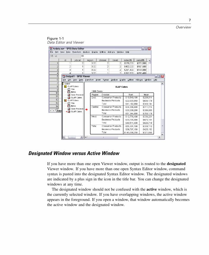
Figure 1-1Data Editor and Viewer

Designated Window versus Active Window

If you have more than one open Viewer window, output is routed to the designatedViewer window. If you have more than one open Syntax Editor window, commandsyntax is pasted into the designated Syntax Editor window. The designated windowsare indicated by a plus sign in the icon in the title bar. You can change the designatedwindows at any time.

The designated window should not be confused with the active window, which isthe currently selected window. If you have overlapping windows, the active windowappears in the foreground. If you open a window, that window automatically becomesthe active window and the designated window.

8

Chapter 1

Changing the Designated Window

E Make the window that you want to designate the active window (click anywhere inthe window).

E Click the Designate Window button on the toolbar (the plus sign icon).

or

E From the menus choose:Utilities

Designate Window

Note: For Data Editor windows, the active Data Editor window determines the datasetthat is used in subsequent calculations or analyses. There is no “designated” DataEditor window. For more information, see “Basic Handling of Multiple Data Sources”in Chapter 6 on p. 108.

Menus

Many of the tasks that you want to perform with SPSS are available through menuselections. Each window in SPSS has its own menu bar with menu selections that areappropriate for that window type.

The Analyze and Graphs menus are available in all windows, making it easy togenerate new output without having to switch windows.

Status Bar

The status bar at the bottom of each SPSS window provides the following information:

Command status. For each procedure or command that you run, a case counter indicatesthe number of cases processed so far. For statistical procedures that require iterativeprocessing, the number of iterations is displayed.

Filter status. If you have selected a random sample or a subset of cases for analysis, themessage Filter on indicates that some type of case filtering is currently in effect andnot all cases in the data file are included in the analysis.

Weight status. The message Weight on indicates that a weight variable is being used toweight cases for analysis.

9

Overview

Split File status. The message Split File on indicates that the data file has been split intoseparate groups for analysis, based on the values of one or more grouping variables.

Showing and Hiding the Status Bar

E From the menus choose:View

Status Bar

Dialog Boxes

Most menu selections open dialog boxes. You use dialog boxes to select variablesand options for analysis.

Dialog boxes for statistical procedures and charts typically have two basic components:

Source variable list. A list of variables in the active dataset. Only variable types that areallowed by the selected procedure are displayed in the source list. Use of short stringand long string variables is restricted in many procedures.

Target variable list(s). One or more lists indicating the variables that you have chosenfor the analysis, such as dependent and independent variable lists.

Variable Names and Variable Labels in Dialog Box Lists

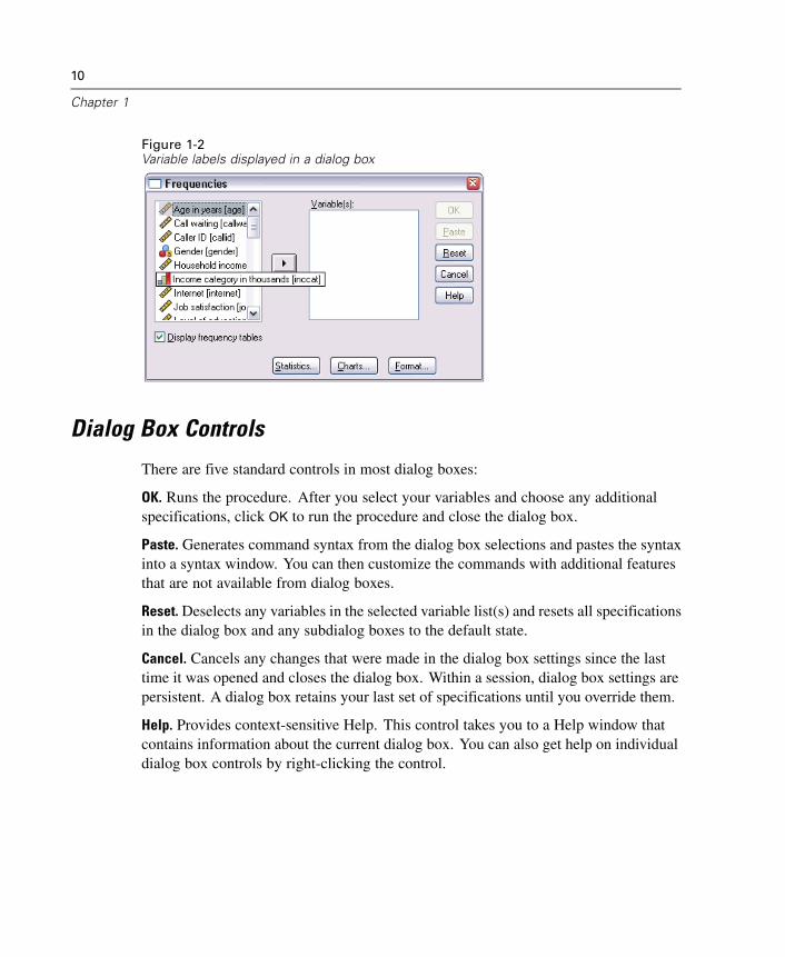
You can display either variable names or variable labels in dialog box lists.

To control the display of variable names or labels, choose Options from the Editmenu in any window.

To define or modify variable labels, use Variable View in the Data Editor.

For data that are imported from database sources, field names are used as variablelabels.

For long labels, position the mouse pointer over the label in the list to view theentire label.

If no variable label is defined, the variable name is displayed.

10

Chapter 1

Figure 1-2Variable labels displayed in a dialog box

Dialog Box Controls

There are five standard controls in most dialog boxes:

OK. Runs the procedure. After you select your variables and choose any additionalspecifications, click OK to run the procedure and close the dialog box.

Paste. Generates command syntax from the dialog box selections and pastes the syntaxinto a syntax window. You can then customize the commands with additional featuresthat are not available from dialog boxes.

Reset. Deselects any variables in the selected variable list(s) and resets all specificationsin the dialog box and any subdialog boxes to the default state.

Cancel. Cancels any changes that were made in the dialog box settings since the lasttime it was opened and closes the dialog box. Within a session, dialog box settings arepersistent. A dialog box retains your last set of specifications until you override them.

Help. Provides context-sensitive Help. This control takes you to a Help window thatcontains information about the current dialog box. You can also get help on individualdialog box controls by right-clicking the control.

11

Overview

Subdialog Boxes

Because most procedures provide a great deal of flexibility, not all of the possiblechoices can be contained in a single dialog box. The main dialog box usually containsthe minimum information that is required to run a procedure. Additional specificationsare made in subdialog boxes.

In the main dialog box, controls with an ellipsis (...) after the name indicate that asubdialog box will be displayed.

Selecting Variables

To select a single variable, simply highlight it on the source variable list and click theright arrow button next to the target variable list. If there is only one target variablelist, you can double-click individual variables to move them from the source list tothe target list.

You can also select multiple variables:

To select multiple variables that are grouped together on the variable list, click thefirst variable and then Shift-click the last variable in the group.

To select multiple variables that are not grouped together on the variable list, clickthe first variable, then Ctrl-click the next variable, and so on.

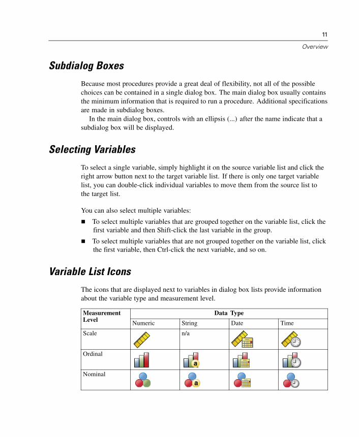
Variable List Icons

The icons that are displayed next to variables in dialog box lists provide informationabout the variable type and measurement level.

Data TypeMeasurementLevel Numeric String Date Time

Scale n/a

Ordinal

Nominal

12

Chapter 1

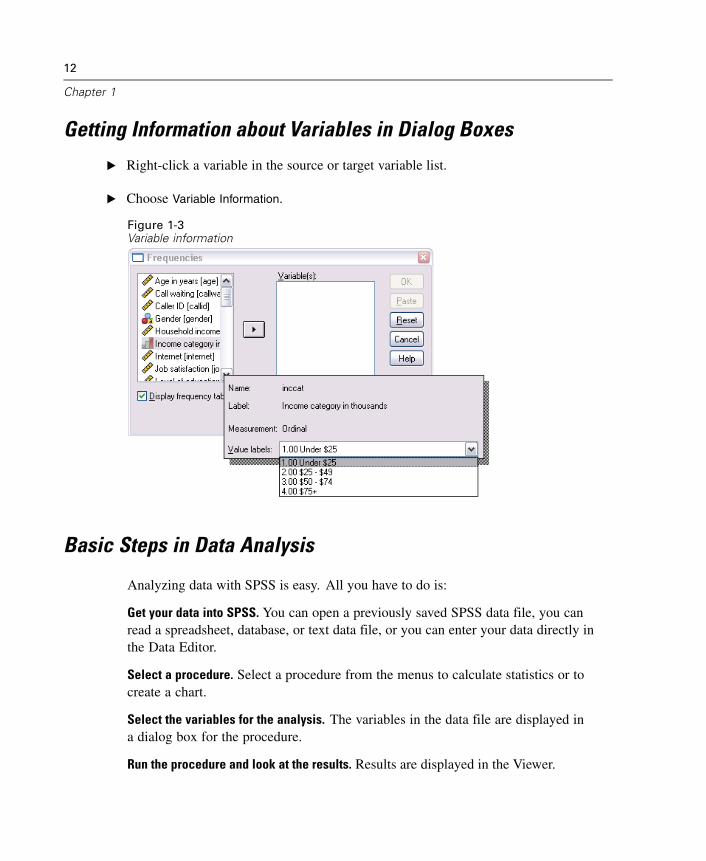
Getting Information about Variables in Dialog Boxes

E Right-click a variable in the source or target variable list.

E Choose Variable Information.

Figure 1-3Variable information

Basic Steps in Data Analysis

Analyzing data with SPSS is easy. All you have to do is:

Get your data into SPSS. You can open a previously saved SPSS data file, you canread a spreadsheet, database, or text data file, or you can enter your data directly inthe Data Editor.

Select a procedure. Select a procedure from the menus to calculate statistics or tocreate a chart.

Select the variables for the analysis. The variables in the data file are displayed ina dialog box for the procedure.

Run the procedure and look at the results. Results are displayed in the Viewer.

13

Overview

Statistics Coach

If you are unfamiliar with SPSS or with the statistical procedures that are availablein SPSS, the Statistics Coach can help you get started by prompting you with simplequestions, nontechnical language, and visual examples that help you select the basicstatistical and charting features that are best suited for your data.

To use the Statistics Coach, from the menus in any SPSS window choose:Help

Statistics Coach

The Statistics Coach covers only a selected subset of procedures in the SPSS Basesystem. It is designed to provide general assistance for many of the basic, commonlyused statistical techniques.

Finding Out More about SPSS

For a comprehensive overview of SPSS basics, see the online tutorial. From any SPSSmenu choose:Help

Tutorial

Chapter

2Getting Help

Help is provided in many different forms:

Help menu. The Help menu in most SPSS windows provides access to the main Helpsystem, plus tutorials and technical reference material.

Topics. Provides access to the Contents, Index, and Search tabs, which you canuse to find specific Help topics.

Tutorial. Illustrated, step-by-step instructions on how to use many of the basicfeatures in SPSS. You don’t have to view the whole tutorial from start to finish.You can choose the topics you want to view, skip around and view topics in anyorder, and use the index or table of contents to find specific topics.

Case Studies. Hands-on examples of how to create various types of statisticalanalyses and how to interpret the results. The sample data files used in theexamples are also provided so that you can work through the examples to seeexactly how the results were produced. You can choose the specific procedure(s)that you want to learn about from the table of contents or search for relevant topicsin the index.

Statistics Coach. A wizard-like approach to guide you through the process offinding the procedure that you want to use. After you make a series of selections,the Statistics Coach opens the dialog box for the statistical, reporting, or chartingprocedure that meets your selected criteria. The Statistics Coach provides accessto most statistical and reporting procedures in the Base system and many chartingprocedures.

15

16

Chapter 2

Command Syntax Reference. Detailed command syntax reference information isavailable in two forms: integrated into the overall Help system and as a separatedocument in PDF form in the SPSS Command Syntax Reference, available fromthe Help menu.

Statistical Algorithms. The algorithms used for most statistical procedures areavailable in PDF form from the Help menu and from the Help topics for theassociated dialog box interface.

Context-sensitive Help. In many places in the user interface, you can getcontext-sensitive Help.

Dialog box Help buttons. Most dialog boxes have a Help button that takes youdirectly to a Help topic for that dialog box. The Help topic provides generalinformation and links to related topics.

Dialog box context menu Help. Many dialog boxes provide context-sensitive Helpfor individual controls and features. Right-click on any control in a dialog box andselect What’s This? from the context menu to display a description of the controland directions for its use. (If What’s This? does not appear on the context menu,then this form of Help is not available for that dialog box.)

Pivot table context menu Help. Right-click on terms in an activated pivot table inthe Viewer and select What’s This? from the context menu to display definitionsof the terms.

Case Studies. Right-click on a pivot table and select Case Studies from the contextmenu to go directly to a detailed example for the procedure that produced thattable. (If Case Studies does not appear on the context menu, then this form ofHelp is not available for that procedure.)

Command syntax. In a command syntax window, position the cursor anywherewithin a syntax block for a command and press F1 on the keyboard. A completecommand syntax chart for that command will be displayed. Complete commandsyntax documentation is available from the links in the list of related topics andfrom the Help Contents tab.

Scripting and OLE automation. In a script window (File menu, New or Open, Script),the Help menu provides access to information on the scripting language and SPSSOLE automation objects, methods, and properties. Context-sensitive Help in ascript window is available with F1 or F2 (object browser).

17

Getting Help

Microsoft Internet Explorer Settings

Most Help features in this application use technology based on Microsoft InternetExplorer. Some versions of Internet Explorer (including the version provided withMicrosoft XP, Service Pack 2) will by default block what it considers “active content”in Internet Explorer windows on your local computer. This default setting may resultin some blocked content in Help features. To see all Help content, you can changethe default behavior of Internet Explorer.

E From the Internet Explorer menus choose:Tools

Internet Options...

E Click the Advanced tab.

E Scroll down to the Security section.

E Select (check) Allow active content to run in files on My Computer.

Other Resources

If you can’t find the information you want in the Help system, these other resourcesmay have the answers you need:

SPSS for Windows Developer’s Guide. Provides information and examples for thedeveloper’s tools included with SPSS for Windows, including OLE automation,third-party API, input/output DLL, Production Facility, and Scripting Facility.The Developer’s Guide is available in PDF form in the SPSS\developer directoryon the installation CD.

Technical Support Web site. Answers to many common problems can be found athttp://support.spss.com. (The Technical Support Web site requires a login IDand password. Information on how to obtain an ID and password is provided atthe URL listed above.)

Using the Help Table of ContentsE In any window, from the menus choose:

HelpTopics

E Click the Contents tab.

18

Chapter 2

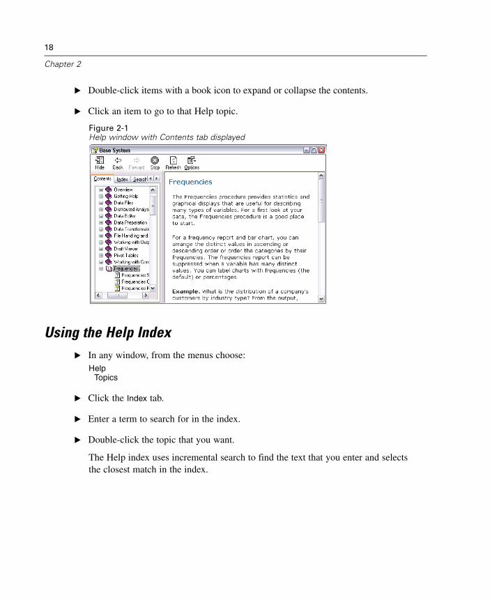
E Double-click items with a book icon to expand or collapse the contents.

E Click an item to go to that Help topic.

Figure 2-1Help window with Contents tab displayed

Using the Help IndexE In any window, from the menus choose:

HelpTopics

E Click the Index tab.

E Enter a term to search for in the index.

E Double-click the topic that you want.

The Help index uses incremental search to find the text that you enter and selectsthe closest match in the index.

19

Getting Help

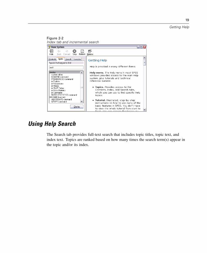
Figure 2-2Index tab and incremental search

Using Help Search

The Search tab provides full-text search that includes topic titles, topic text, andindex text. Topics are ranked based on how many times the search term(s) appear inthe topic and/or its index.

20

Chapter 2

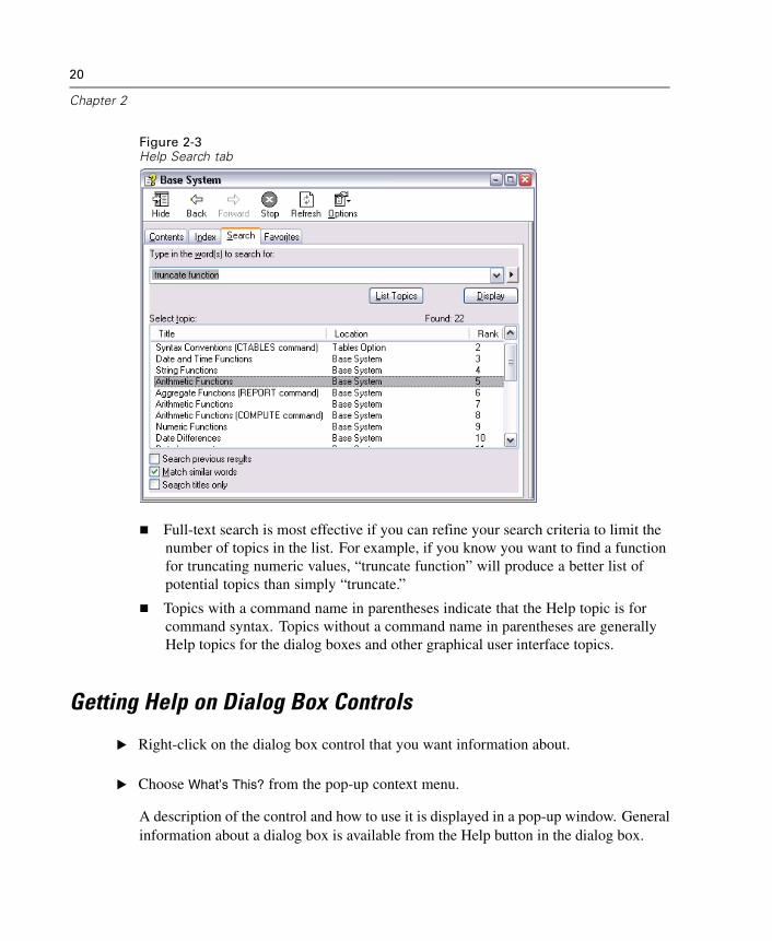
Figure 2-3Help Search tab

Full-text search is most effective if you can refine your search criteria to limit thenumber of topics in the list. For example, if you know you want to find a functionfor truncating numeric values, “truncate function” will produce a better list ofpotential topics than simply “truncate.”

Topics with a command name in parentheses indicate that the Help topic is forcommand syntax. Topics without a command name in parentheses are generallyHelp topics for the dialog boxes and other graphical user interface topics.

Getting Help on Dialog Box Controls

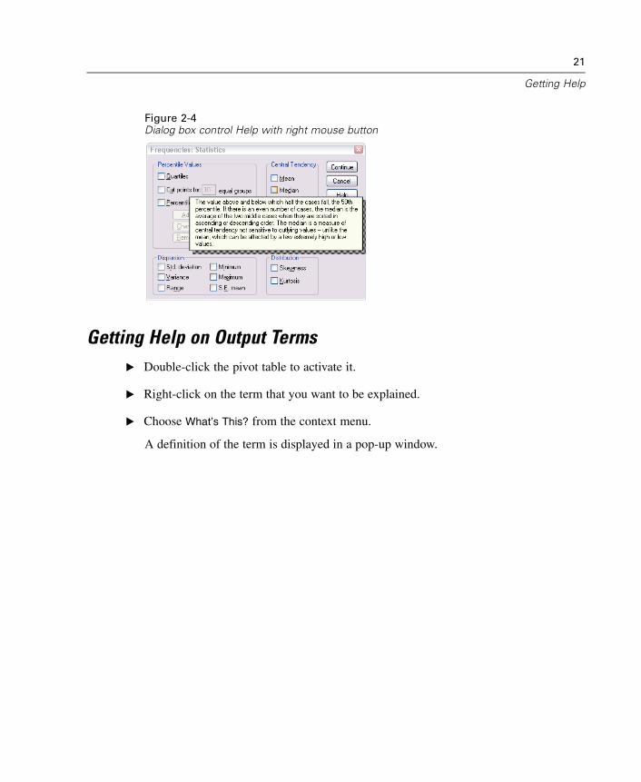
E Right-click on the dialog box control that you want information about.

E Choose What’s This? from the pop-up context menu.

A description of the control and how to use it is displayed in a pop-up window. Generalinformation about a dialog box is available from the Help button in the dialog box.

21

Getting Help

Figure 2-4Dialog box control Help with right mouse button

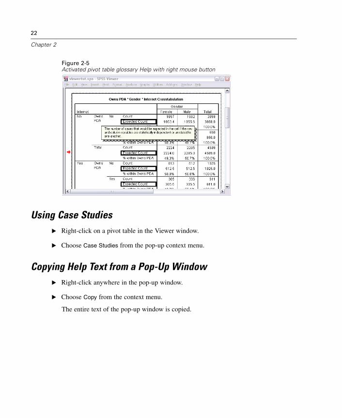
Getting Help on Output TermsE Double-click the pivot table to activate it.

E Right-click on the term that you want to be explained.

E Choose What’s This? from the context menu.

A definition of the term is displayed in a pop-up window.

22

Chapter 2

Figure 2-5Activated pivot table glossary Help with right mouse button

Using Case StudiesE Right-click on a pivot table in the Viewer window.

E Choose Case Studies from the pop-up context menu.

Copying Help Text from a Pop-Up WindowE Right-click anywhere in the pop-up window.

E Choose Copy from the context menu.

The entire text of the pop-up window is copied.

Chapter

3Data Files

Data files come in a wide variety of formats, and this software is designed to handlemany of them, including:

Spreadsheets created with Excel and Lotus

Database tables from many database sources, including Oracle, SQLServer,Access, dBASE, and others

Tab-delimited and other types of simple text files

Data files in SPSS format created on other operating systems

SYSTAT data files

SAS data files

Stata data files

Opening a Data File

In addition to files saved in SPSS format, you can open Excel, SAS, Stata, tab-delimitedand other files without converting the files to an intermediate format or entering datadefinition information.

To Open Data FilesE From the menus choose:

FileOpen

Data...

E In the Open File dialog box, select the file that you want to open.

E Click Open.

23

24

Chapter 3

Optionally, you can:

Read variable names from the first row for spreadsheet and tab-delimited files.

Specify a range of cells to read for spreadsheet files.

Specify a sheet within an Excel file to read (Excel 5 or later).

Data File Types

SPSS. Opens data files saved in SPSS format, including SPSS for Windows, Macintosh,UNIX, and also the DOS product SPSS/PC+.

SPSS/PC+. Opens SPSS/PC+ data files.

SYSTAT. Opens SYSTAT data files.

SPSS Portable. Opens data files saved in SPSS portable format. Saving a file in portableformat takes considerably longer than saving the file in SPSS format.

Excel. Opens Excel files.

Lotus 1-2-3. Opens data files saved in 1-2-3 format for release 3.0, 2.0, or 1A of Lotus.

SYLK. Opens data files saved in SYLK (symbolic link) format, a format used by somespreadsheet applications.

dBASE. Opens dBASE-format files for either dBASE IV, dBASE III or III PLUS,or dBASE II. Each case is a record. Variable and value labels and missing-valuespecifications are lost when you save a file in this format.

SAS Long File Name. SAS versions 7–9 for Windows, long extension.

SAS Short File Name. SAS versions 7–9 for Windows, short extension.

SAS v6 for Windows. SAS version 6.08 for Windows and OS2.

SAS v6 for UNIX. SAS version 6 for UNIX (Sun, HP, IBM).

SAS Transport. SAS transport file.

Stata. Stata versions 4–8.

Text. ASCII text file.

25

Data Files

Opening File Options

Read variable names. For spreadsheets, you can read variable names from the first rowof the file or the first row of the defined range. The values are converted as necessaryto create valid variable names, including converting spaces to underscores.

Worksheet. Excel 5 or later files can contain multiple worksheets. By default, the DataEditor reads the first worksheet. To read a different worksheet, select the worksheetfrom the drop-down list.

Range. For spreadsheet data files, you can also read a range of cells. Use the samemethod for specifying cell ranges as you would with the spreadsheet application.

Reading Excel 5 or Later Files

The following rules apply to reading Excel 5 or later files:

Data type and width. Each column is a variable. The data type and width for eachvariable are determined by the data type and width in the Excel file. If the columncontains more than one data type (for example, date and numeric), the data type is setto string, and all values are read as valid string values.

Blank cells. For numeric variables, blank cells are converted to the system-missingvalue, indicated by a period. For string variables, a blank is a valid string value, andblank cells are treated as valid string values.

Variable names. If you read the first row of the Excel file (or the first row of thespecified range) as variable names, values that don’t conform to variable naming rulesare converted to valid variable names, and the original names are used as variablelabels. If you do not read variable names from the Excel file, default variable namesare assigned.

26

Chapter 3

Reading Older Excel Files and Other Spreadsheets

The following rules apply to reading Excel files prior to version 5 and other spreadsheetdata:

Data type and width. The data type and width for each variable are determined by thecolumn width and data type of the first data cell in the column. Values of other typesare converted to the system-missing value. If the first data cell in the column is blank,the global default data type for the spreadsheet (usually numeric) is used.

Blank cells. For numeric variables, blank cells are converted to the system-missingvalue, indicated by a period. For string variables, a blank is a valid string value, andblank cells are treated as valid string values.

Variable names. If you do not read variable names from the spreadsheet, the columnletters (A, B, C, ...) are used for variable names for Excel and Lotus files. For SYLKfiles and Excel files saved in R1C1 display format, the software uses the columnnumber preceded by the letter C for variable names (C1, C2, C3, ...).

Reading dBASE Files

Database files are logically very similar to SPSS-format data files. The followinggeneral rules apply to dBASE files:

Field names are converted to valid variable names.

Colons used in dBASE field names are translated to underscores.

Records marked for deletion but not actually purged are included. The softwarecreates a new string variable, D_R, which contains an asterisk for cases markedfor deletion.

Reading Stata Files

The following general rules apply to Stata data files:

Variable names. Stata variable names are converted to SPSS variable namesin case-sensitive form. Stata variable names that are identical except for caseare converted to valid SPSS variable names by appending an underscore and asequential letter (_A, _B, _C, ..., _Z, _AA, _AB, ..., etc.).

Variable labels. Stata variable labels are converted to SPSS variable labels.

27

Data Files

Value labels. Stata value labels are converted to SPSS value labels, except for Statavalue labels assigned to “extended” missing values.

Missing values. Stata “extended” missing values are converted to system-missing.

Data conversion. Stata date format values are converted to SPSS DATE format(d-m-y) values. Stata “time-series” date format values (weeks, months, quarters,etc.) are converted to simple numeric (F) format, preserving the original, internalinteger value which is the number of weeks, months, quarters, etc., since the startof 1960.

Reading Database Files

You can read data from any database format for which you have a database driver. Inlocal analysis mode, the necessary drivers must be installed on your local computer. Indistributed analysis mode (available with SPSS Server), the drivers must be installedon the remote server. For more information, see “Distributed Analysis Mode” inChapter 4 on p. 73.

To Read Database Files

E From the menus choose:File

Open DatabaseNew Query...

E Select the data source.

E If necessary (depending on the data source), select the database file and/or enter a loginname, password, and other information.

E Select the table(s) and fields. (For OLE DB data sources, you can only select one table.)

E Specify any relationships between your tables.

E Optionally:

Specify any selection criteria for your data.

Add a prompt for user input to create a parameter query.

Save your constructed query before running it.

28

Chapter 3

To Edit Saved Database Queries


Open DatabaseEdit Query...

E Select the query file (*.spq) that you want to edit.

E Follow the instructions for creating a new query.

To Read Database Files with Saved Queries


Open DatabaseRun Query...

E Select the query file (*.spq) that you want to run.

E If necessary (depending on the database file), enter a login name and password.

E If the query has an embedded prompt, enter other information if necessary (forexample, the quarter for which you want to retrieve sales figures).

Selecting a Data Source

Use the first screen of the Database Wizard to select the type of data source to read.

ODBC Data Sources

If you do not have any ODBC data sources configured, or if you want to add a newdata source, click Add ODBC Data Source. In distributed analysis mode (available withSPSS Server), this button is not available. To add data sources in distributed analysismode, see your system administrator.

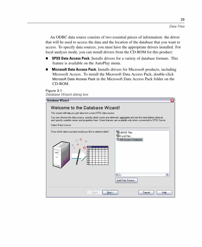
29

Data Files

An ODBC data source consists of two essential pieces of information: the driverthat will be used to access the data and the location of the database that you want toaccess. To specify data sources, you must have the appropriate drivers installed. Forlocal analysis mode, you can install drivers from the CD-ROM for this product:

SPSS Data Access Pack. Installs drivers for a variety of database formats. Thisfeature is available on the AutoPlay menu.

Microsoft Data Access Pack. Installs drivers for Microsoft products, includingMicrosoft Access. To install the Microsoft Data Access Pack, double-clickMicrosoft Data Access Pack in the Microsoft Data Access Pack folder on theCD-ROM.

Figure 3-1Database Wizard dialog box

30

Chapter 3

OLE DB Data Sources

To access OLE DB data sources, you must have the following items installed on thecomputer that is running SPSS:

.NET framework

Dimensions Data Model and OLE DB Access

Versions of these components that are compatible with this release of SPSS can beinstalled from the SPSS installation CD and are available on the AutoPlay menu.

You can only add OLE DB data sources in local analysis mode. To add OLEDB data sources in distributed analysis mode on a Windows server, consult yoursystem administrator.

In distributed analysis mode (available with SPSS Server), OLE DB data sourcesare only available on Windows servers, and both .NET and the Dimensions DataModel and OLE DB Access must be installed on the server.

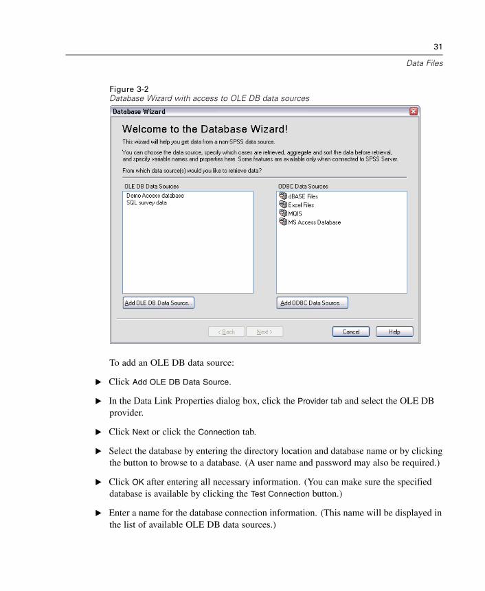
31

Data Files

Figure 3-2Database Wizard with access to OLE DB data sources

To add an OLE DB data source:

E Click Add OLE DB Data Source.

E In the Data Link Properties dialog box, click the Provider tab and select the OLE DBprovider.

E Click Next or click the Connection tab.

E Select the database by entering the directory location and database name or by clickingthe button to browse to a database. (A user name and password may also be required.)

E Click OK after entering all necessary information. (You can make sure the specifieddatabase is available by clicking the Test Connection button.)

E Enter a name for the database connection information. (This name will be displayed inthe list of available OLE DB data sources.)

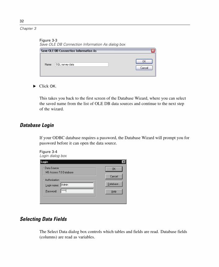
32

Chapter 3

Figure 3-3Save OLE DB Connection Information As dialog box

E Click OK.

This takes you back to the first screen of the Database Wizard, where you can selectthe saved name from the list of OLE DB data sources and continue to the next stepof the wizard.

Database Login

If your ODBC database requires a password, the Database Wizard will prompt you forpassword before it can open the data source.

Figure 3-4Login dialog box

Selecting Data Fields

The Select Data dialog box controls which tables and fields are read. Database fields(columns) are read as variables.

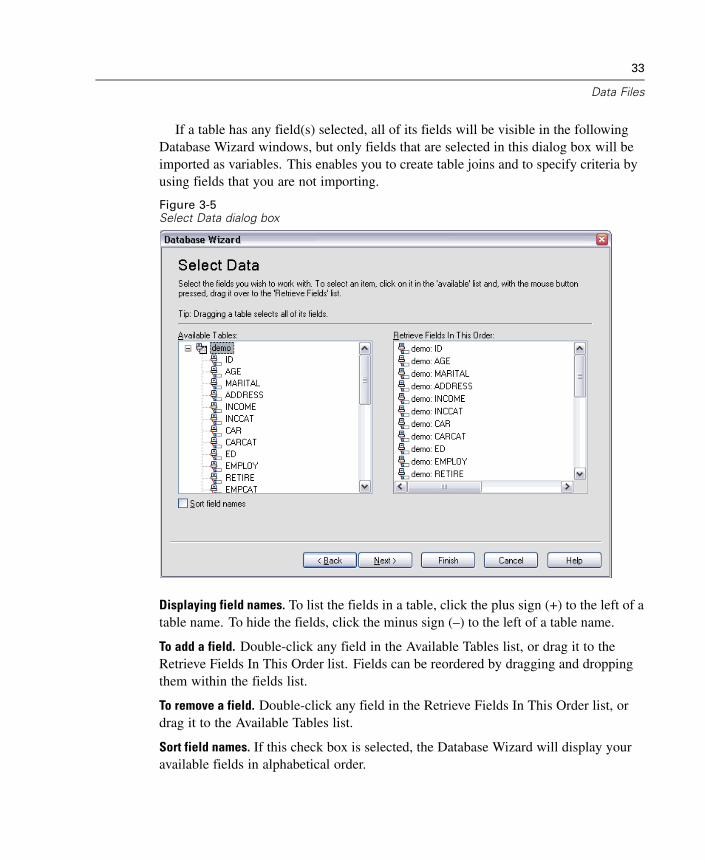
33

Data Files

If a table has any field(s) selected, all of its fields will be visible in the followingDatabase Wizard windows, but only fields that are selected in this dialog box will beimported as variables. This enables you to create table joins and to specify criteria byusing fields that you are not importing.

Figure 3-5Select Data dialog box

Displaying field names. To list the fields in a table, click the plus sign (+) to the left of atable name. To hide the fields, click the minus sign (–) to the left of a table name.

To add a field. Double-click any field in the Available Tables list, or drag it to theRetrieve Fields In This Order list. Fields can be reordered by dragging and droppingthem within the fields list.

To remove a field. Double-click any field in the Retrieve Fields In This Order list, ordrag it to the Available Tables list.

Sort field names. If this check box is selected, the Database Wizard will display youravailable fields in alphabetical order.

34

Chapter 3

Note: For OLE DB data sources, you can select fields only from a single table.Multiple table joins are not supported for OLE DB data sources.

Creating a Relationship between Tables

The Specify Relationships dialog box allows you to define the relationships betweenthe tables for ODBC data sources. If fields from more than one table are selected,you must define at least one join.

Figure 3-6Specify Relationships dialog box

Establishing relationships. To create a relationship, drag a field from any table onto thefield to which you want to join it. The Database Wizard will draw a join line betweenthe two fields, indicating their relationship. These fields must be of the same data type.

Auto Join Tables. Attempts to automatically join tables based on primary/foreign keysor matching field names and data type.

35

Data Files

Specifying join types. If outer joins are supported by your driver, you can specify innerjoins, left outer joins, or right outer joins. To select the type of join, double-click thejoin line between the fields, and the wizard will display the Relationship Propertiesdialog box.

Relationship Properties

This dialog box allows you to specify which type of relationship joins your tables.

Figure 3-7Relationship Properties dialog box

Inner joins. An inner join includes only rows where the related fields are equal. In thisexample, all rows with matching ID values in the two tables will be included.

Outer joins. In addition to one-to-one matching with inner joins, you can also useouter joins to merge tables with a one-to-many matching scheme. For example, youcould match a table in which there are only a few records representing data values andassociated descriptive labels with values in a table containing hundreds or thousands ofrecords representing survey respondents. A left outer join includes all records from thetable on the left and, from the table on the right, includes only those records in whichthe related fields are equal. In a right outer join, the join imports all records from thetable on the right and, from the table on the left, imports only those records in whichthe related fields are equal.

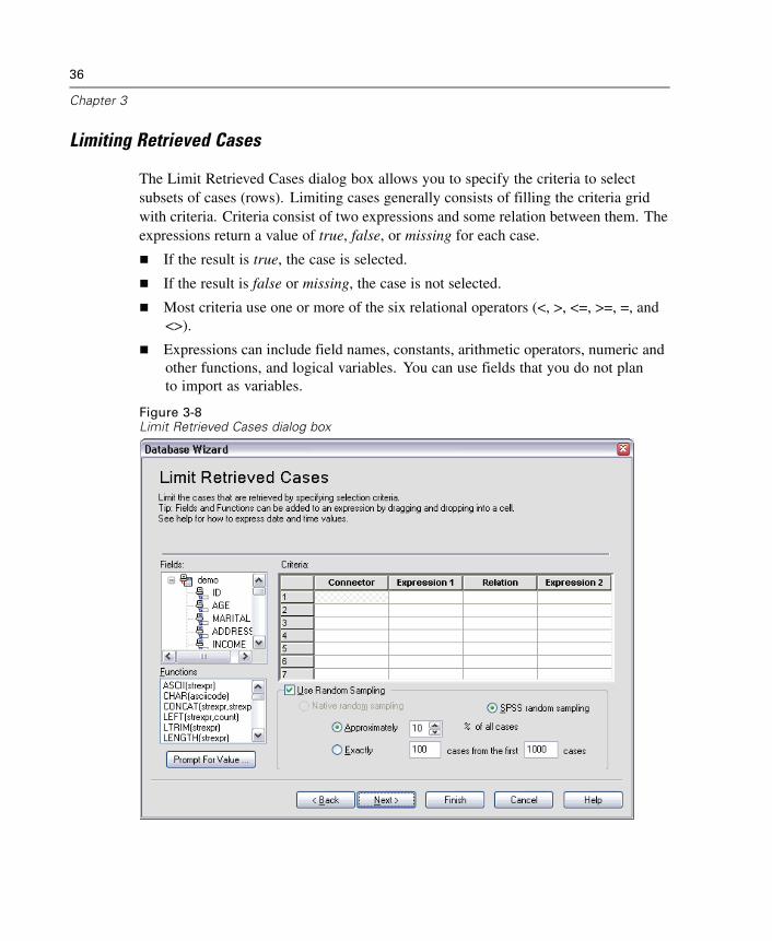
36

Chapter 3

Limiting Retrieved Cases

The Limit Retrieved Cases dialog box allows you to specify the criteria to selectsubsets of cases (rows). Limiting cases generally consists of filling the criteria gridwith criteria. Criteria consist of two expressions and some relation between them. Theexpressions return a value of true, false, or missing for each case.

If the result is true, the case is selected.

If the result is false or missing, the case is not selected.

Most criteria use one or more of the six relational operators (<, >, <=, >=, =, and<>).

Expressions can include field names, constants, arithmetic operators, numeric andother functions, and logical variables. You can use fields that you do not planto import as variables.

Figure 3-8Limit Retrieved Cases dialog box

37

Data Files

To build your criteria, you need at least two expressions and a relation to connectthe expressions.

E To build an expression, choose one of the following methods:

In an Expression cell, type field names, constants, arithmetic operators, numericand other functions, or logical variables.

Double-click the field in the Fields list.

Drag the field from the Fields list to an Expression cell.

Choose a field from the drop-down menu in any active Expression cell.

E To choose the relational operator (such as = or >), put your cursor in the Relation celland either type the operator or choose it from the drop-down menu.

Dates and times in expressions need to be specified in a special manner (including thecurly braces that are shown in the examples):

Date literals should be specified by using the general form: {d yyyy-mm-dd}.

Time literals should be specified by using the general form: {t hh:mm:ss}.

Date/time literals (timestamps) should be specified by using the general form: {dtyyyy-mm-dd hh:mm:ss}.

Functions. A selection of built-in arithmetic, logical, string, date, and time SQLfunctions is provided. You can drag a function from the list into the expression, or youcan enter any valid SQL function. See your database documentation for valid SQLfunctions. A list of standard functions is available at:

http://msdn.microsoft.com/library/en-us/odbc/htm/odbcscalar_functions.asp

Use Random Sampling. This option selects a random sample of cases from the datasource. For large data sources, you may want to limit the number of cases to a small,representative sample, which can significantly reduce the time that it takes to runprocedures. Native random sampling, if available for the data source, is faster thanSPSS random sampling, because SPSS random sampling must still read the entiredata source to extract a random sample.

Approximately. Generates a random sample of approximately the specifiedpercentage of cases. Since this routine makes an independent pseudo-randomdecision for each case, the percentage of cases selected can only approximate





38

Chapter 3

the specified percentage. The more cases there are in the data file, the closer thepercentage of cases selected is to the specified percentage.

Exactly. Selects a random sample of the specified number of cases from thespecified total number of cases. If the total number of cases specified exceedsthe total number of cases in the data file, the sample will contain proportionallyfewer cases than the requested number.

Note: If you use random sampling, aggregation (available in distributed mode withSPSS Server) is not available.

Prompt For Value. You can embed a prompt in your query to create a parameter query.When users run the query, they will be asked to enter information (based on what isspecified here). You might want to do this if you need to see different views of thesame data. For example, you may want to run the same query to see sales figures fordifferent fiscal quarters.

E Place your cursor in any Expression cell, and click Prompt For Value to create a prompt.

Creating a Parameter Query

Use the Prompt for Value dialog box to create a dialog box that solicits informationfrom users each time someone runs your query. This feature is useful if you want toquery the same data source by using different criteria.

Figure 3-9Prompt for Value dialog box

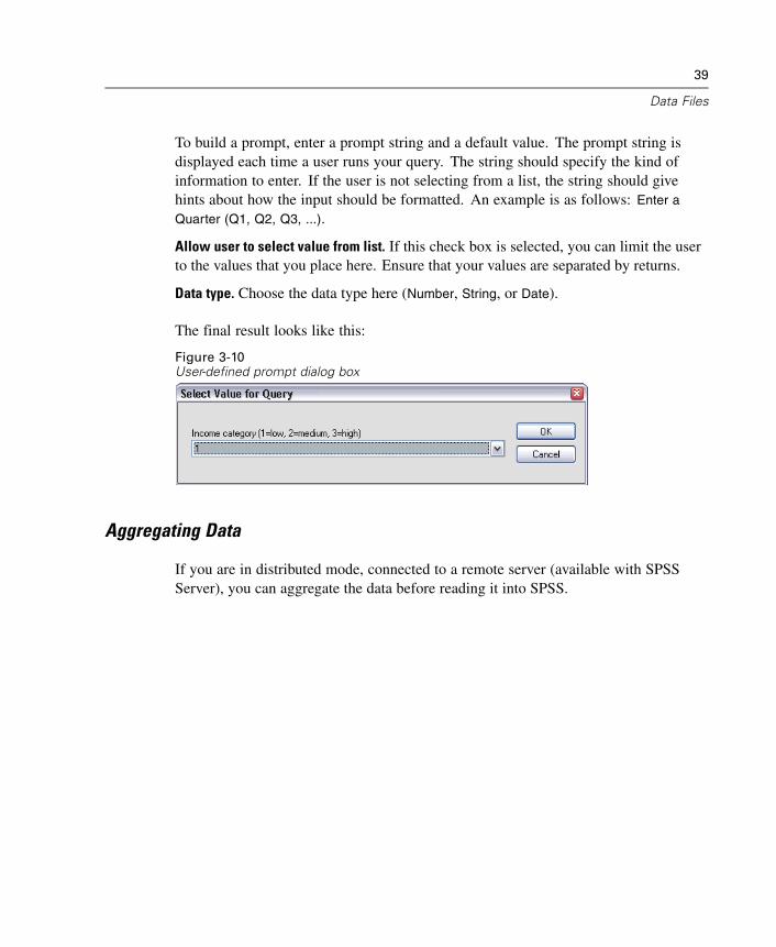
39

Data Files

To build a prompt, enter a prompt string and a default value. The prompt string isdisplayed each time a user runs your query. The string should specify the kind ofinformation to enter. If the user is not selecting from a list, the string should givehints about how the input should be formatted. An example is as follows: Enter a

Quarter (Q1, Q2, Q3, ...).

Allow user to select value from list. If this check box is selected, you can limit the userto the values that you place here. Ensure that your values are separated by returns.

Data type. Choose the data type here (Number, String, or Date).

The final result looks like this:

Figure 3-10User-defined prompt dialog box

Aggregating Data

If you are in distributed mode, connected to a remote server (available with SPSSServer), you can aggregate the data before reading it into SPSS.

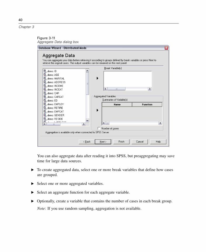
40

Chapter 3

Figure 3-11Aggregate Data dialog box

You can also aggregate data after reading it into SPSS, but preaggregating may savetime for large data sources.

E To create aggregated data, select one or more break variables that define how casesare grouped.

E Select one or more aggregated variables.

E Select an aggregate function for each aggregate variable.

E Optionally, create a variable that contains the number of cases in each break group.

Note: If you use random sampling, aggregation is not available.

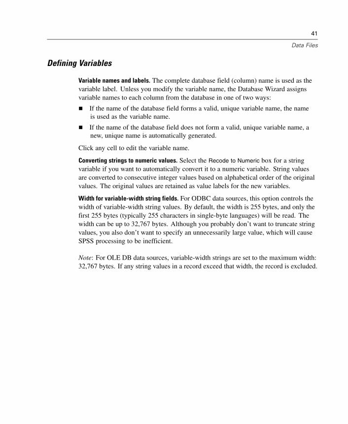
41

Data Files

Defining Variables

Variable names and labels. The complete database field (column) name is used as thevariable label. Unless you modify the variable name, the Database Wizard assignsvariable names to each column from the database in one of two ways:

If the name of the database field forms a valid, unique variable name, the nameis used as the variable name.

If the name of the database field does not form a valid, unique variable name, anew, unique name is automatically generated.

Click any cell to edit the variable name.

Converting strings to numeric values. Select the Recode to Numeric box for a stringvariable if you want to automatically convert it to a numeric variable. String valuesare converted to consecutive integer values based on alphabetical order of the originalvalues. The original values are retained as value labels for the new variables.

Width for variable-width string fields. For ODBC data sources, this option controls thewidth of variable-width string values. By default, the width is 255 bytes, and only thefirst 255 bytes (typically 255 characters in single-byte languages) will be read. Thewidth can be up to 32,767 bytes. Although you probably don’t want to truncate stringvalues, you also don’t want to specify an unnecessarily large value, which will causeSPSS processing to be inefficient.

Note: For OLE DB data sources, variable-width strings are set to the maximum width:32,767 bytes. If any string values in a record exceed that width, the record is excluded.

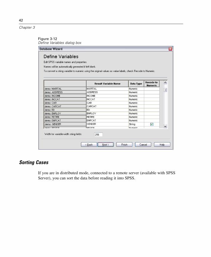
42

Chapter 3

Figure 3-12Define Variables dialog box

Sorting Cases

If you are in distributed mode, connected to a remote server (available with SPSSServer), you can sort the data before reading it into SPSS.

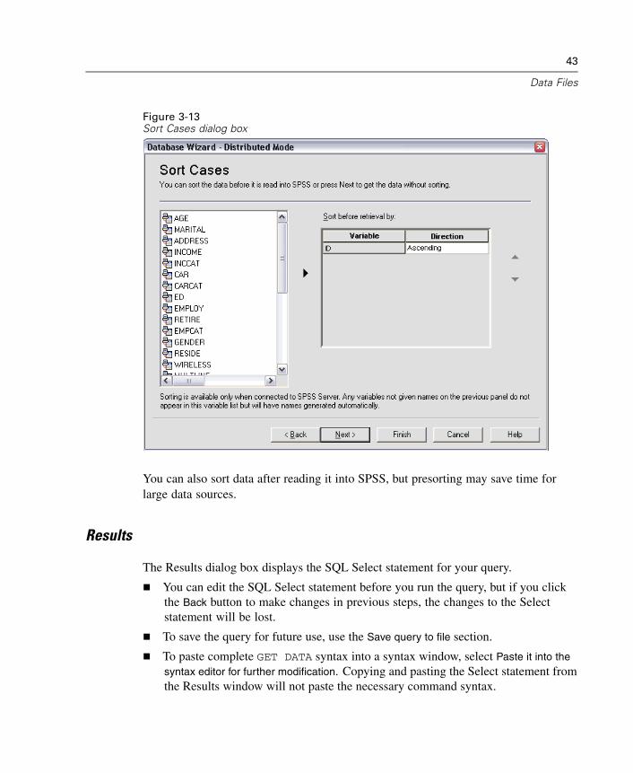
43

Data Files

Figure 3-13Sort Cases dialog box

You can also sort data after reading it into SPSS, but presorting may save time forlarge data sources.

Results

The Results dialog box displays the SQL Select statement for your query.

You can edit the SQL Select statement before you run the query, but if you clickthe Back button to make changes in previous steps, the changes to the Selectstatement will be lost.

To save the query for future use, use the Save query to file section.

To paste complete GET DATA syntax into a syntax window, select Paste it into thesyntax editor for further modification. Copying and pasting the Select statement fromthe Results window will not paste the necessary command syntax.

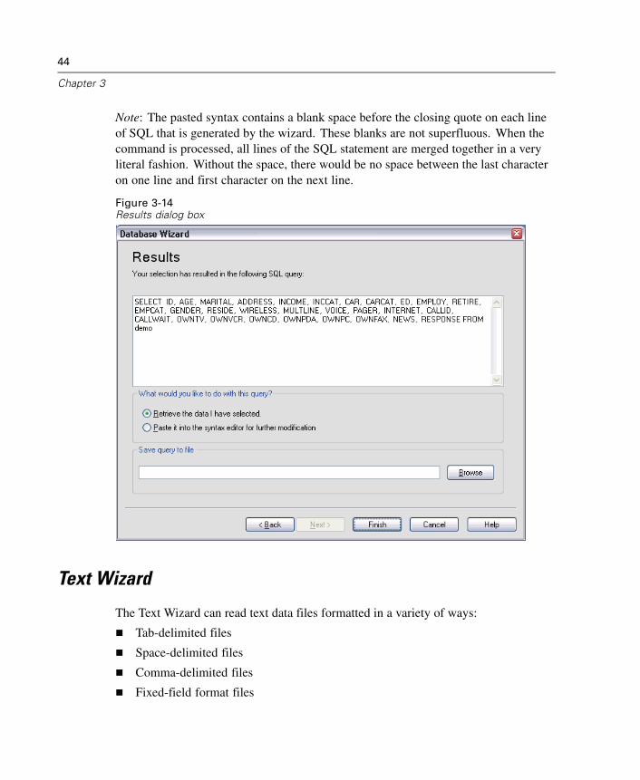
44

Chapter 3

Note: The pasted syntax contains a blank space before the closing quote on each lineof SQL that is generated by the wizard. These blanks are not superfluous. When thecommand is processed, all lines of the SQL statement are merged together in a veryliteral fashion. Without the space, there would be no space between the last characteron one line and first character on the next line.

Figure 3-14Results dialog box

Text Wizard

The Text Wizard can read text data files formatted in a variety of ways:

Tab-delimited files

Space-delimited files

Comma-delimited files

Fixed-field format files

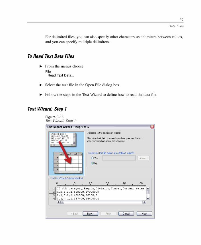
45

Data Files

For delimited files, you can also specify other characters as delimiters between values,and you can specify multiple delimiters.

To Read Text Data Files


Read Text Data...

E Select the text file in the Open File dialog box.

E Follow the steps in the Text Wizard to define how to read the data file.

Text Wizard: Step 1

Figure 3-15Text Wizard: Step 1

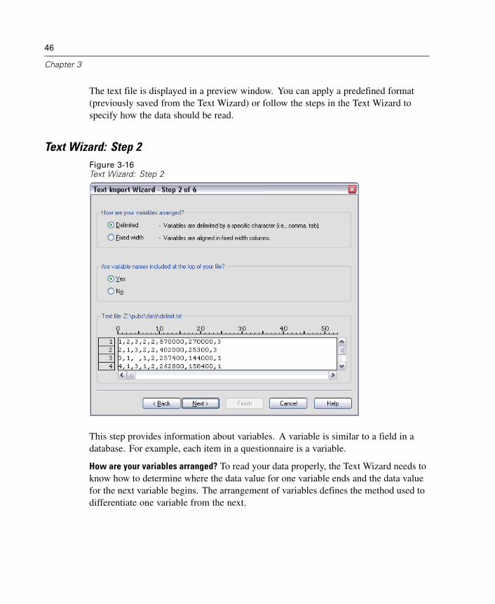
46

Chapter 3

The text file is displayed in a preview window. You can apply a predefined format(previously saved from the Text Wizard) or follow the steps in the Text Wizard tospecify how the data should be read.

Text Wizard: Step 2Figure 3-16Text Wizard: Step 2

This step provides information about variables. A variable is similar to a field in adatabase. For example, each item in a questionnaire is a variable.

How are your variables arranged? To read your data properly, the Text Wizard needs toknow how to determine where the data value for one variable ends and the data valuefor the next variable begins. The arrangement of variables defines the method used todifferentiate one variable from the next.

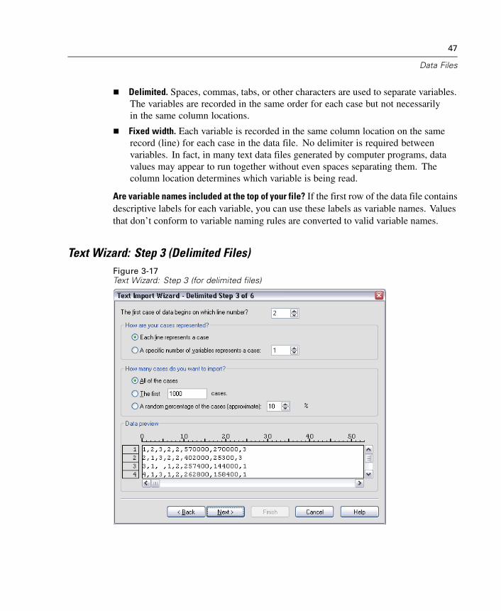
47

Data Files

Delimited. Spaces, commas, tabs, or other characters are used to separate variables.The variables are recorded in the same order for each case but not necessarilyin the same column locations.

Fixed width. Each variable is recorded in the same column location on the samerecord (line) for each case in the data file. No delimiter is required betweenvariables. In fact, in many text data files generated by computer programs, datavalues may appear to run together without even spaces separating them. Thecolumn location determines which variable is being read.

Are variable names included at the top of your file? If the first row of the data file containsdescriptive labels for each variable, you can use these labels as variable names. Valuesthat don’t conform to variable naming rules are converted to valid variable names.

Text Wizard: Step 3 (Delimited Files)Figure 3-17Text Wizard: Step 3 (for delimited files)

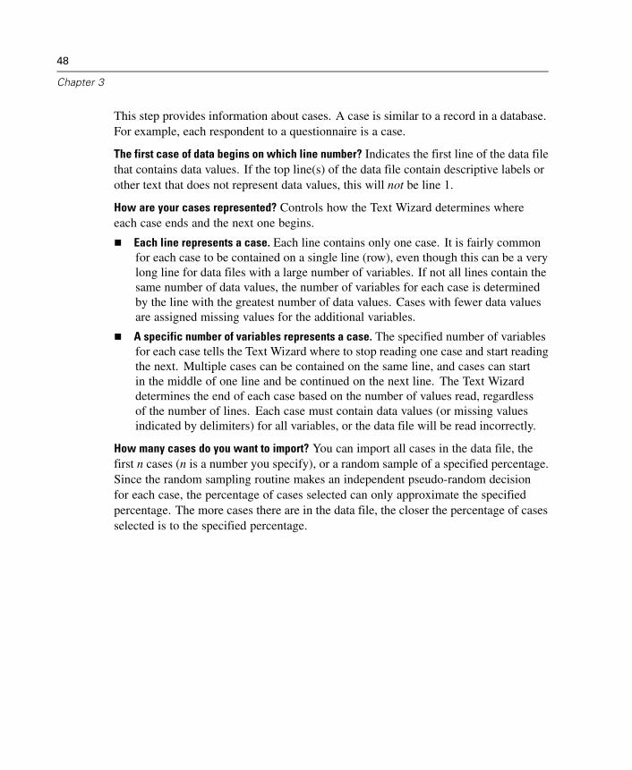
48

Chapter 3

This step provides information about cases. A case is similar to a record in a database.For example, each respondent to a questionnaire is a case.

The first case of data begins on which line number? Indicates the first line of the data filethat contains data values. If the top line(s) of the data file contain descriptive labels orother text that does not represent data values, this will not be line 1.

How are your cases represented? Controls how the Text Wizard determines whereeach case ends and the next one begins.

Each line represents a case. Each line contains only one case. It is fairly commonfor each case to be contained on a single line (row), even though this can be a verylong line for data files with a large number of variables. If not all lines contain thesame number of data values, the number of variables for each case is determinedby the line with the greatest number of data values. Cases with fewer data valuesare assigned missing values for the additional variables.

A specific number of variables represents a case. The specified number of variablesfor each case tells the Text Wizard where to stop reading one case and start readingthe next. Multiple cases can be contained on the same line, and cases can startin the middle of one line and be continued on the next line. The Text Wizarddetermines the end of each case based on the number of values read, regardlessof the number of lines. Each case must contain data values (or missing valuesindicated by delimiters) for all variables, or the data file will be read incorrectly.

How many cases do you want to import? You can import all cases in the data file, thefirst n cases (n is a number you specify), or a random sample of a specified percentage.Since the random sampling routine makes an independent pseudo-random decisionfor each case, the percentage of cases selected can only approximate the specifiedpercentage. The more cases there are in the data file, the closer the percentage of casesselected is to the specified percentage.

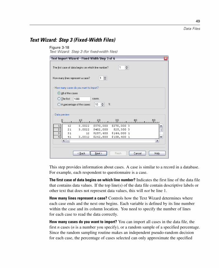
49

Data Files

Text Wizard: Step 3 (Fixed-Width Files)Figure 3-18Text Wizard: Step 3 (for fixed-width files)

This step provides information about cases. A case is similar to a record in a database.For example, each respondent to questionnaire is a case.

The first case of data begins on which line number? Indicates the first line of the data filethat contains data values. If the top line(s) of the data file contain descriptive labels orother text that does not represent data values, this will not be line 1.

How many lines represent a case? Controls how the Text Wizard determines whereeach case ends and the next one begins. Each variable is defined by its line numberwithin the case and its column location. You need to specify the number of linesfor each case to read the data correctly.

How many cases do you want to import? You can import all cases in the data file, thefirst n cases (n is a number you specify), or a random sample of a specified percentage.Since the random sampling routine makes an independent pseudo-random decisionfor each case, the percentage of cases selected can only approximate the specified

50

Chapter 3

percentage. The more cases there are in the data file, the closer the percentage of casesselected is to the specified percentage.

Text Wizard: Step 4 (Delimited Files)Figure 3-19Text Wizard: Step 4 (for delimited files)

This step displays the Text Wizard’s best guess on how to read the data file and allowsyou to modify how the Text Wizard will read variables from the data file.

Which delimiters appear between variables? Indicates the characters or symbols thatseparate data values. You can select any combination of spaces, commas, semicolons,tabs, or other characters. Multiple, consecutive delimiters without intervening datavalues are treated as missing values.

What is the text qualifier? Characters used to enclose values that contain delimitercharacters. For example, if a comma is the delimiter, values that contain commas willbe read incorrectly unless there is a text qualifier enclosing the value, preventing the

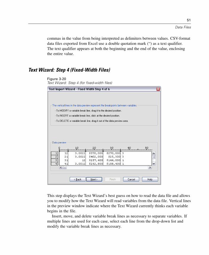
51

Data Files

commas in the value from being interpreted as delimiters between values. CSV-formatdata files exported from Excel use a double quotation mark (“) as a text qualifier.The text qualifier appears at both the beginning and the end of the value, enclosingthe entire value.

Text Wizard: Step 4 (Fixed-Width Files)

Figure 3-20Text Wizard: Step 4 (for fixed-width files)

This step displays the Text Wizard’s best guess on how to read the data file and allowsyou to modify how the Text Wizard will read variables from the data file. Vertical linesin the preview window indicate where the Text Wizard currently thinks each variablebegins in the file.

Insert, move, and delete variable break lines as necessary to separate variables. Ifmultiple lines are used for each case, select each line from the drop-down list andmodify the variable break lines as necessary.

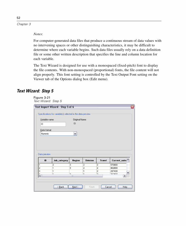
52

Chapter 3

Notes:

For computer-generated data files that produce a continuous stream of data values withno intervening spaces or other distinguishing characteristics, it may be difficult todetermine where each variable begins. Such data files usually rely on a data definitionfile or some other written description that specifies the line and column location foreach variable.

The Text Wizard is designed for use with a monospaced (fixed-pitch) font to displaythe file contents. With non-monospaced (proportional) fonts, the file content will notalign properly. This font setting is controlled by the Text Output Font setting on theViewer tab of the Options dialog box (Edit menu).


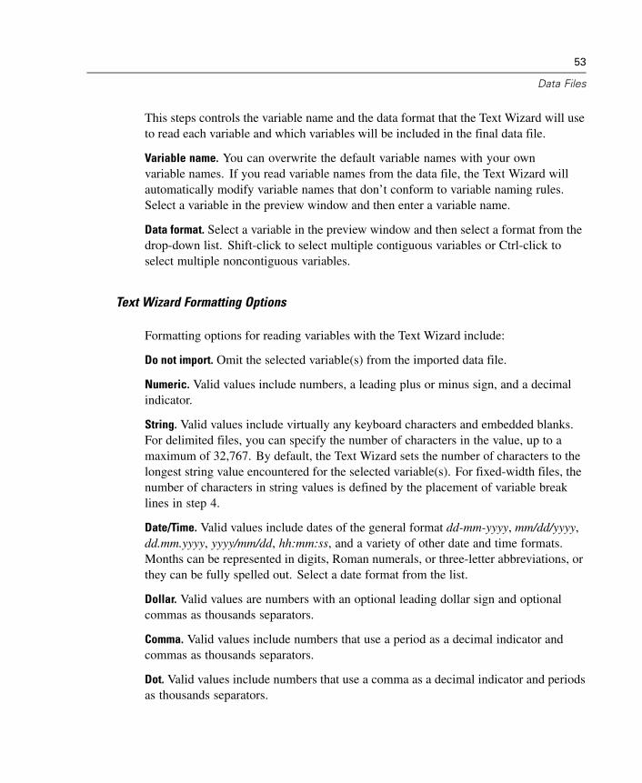
53

Data Files

This steps controls the variable name and the data format that the Text Wizard will useto read each variable and which variables will be included in the final data file.

Variable name. You can overwrite the default variable names with your ownvariable names. If you read variable names from the data file, the Text Wizard willautomatically modify variable names that don’t conform to variable naming rules.Select a variable in the preview window and then enter a variable name.

Data format. Select a variable in the preview window and then select a format from thedrop-down list. Shift-click to select multiple contiguous variables or Ctrl-click toselect multiple noncontiguous variables.

Text Wizard Formatting Options

Formatting options for reading variables with the Text Wizard include:

Do not import. Omit the selected variable(s) from the imported data file.

Numeric. Valid values include numbers, a leading plus or minus sign, and a decimalindicator.

String. Valid values include virtually any keyboard characters and embedded blanks.For delimited files, you can specify the number of characters in the value, up to amaximum of 32,767. By default, the Text Wizard sets the number of characters to thelongest string value encountered for the selected variable(s). For fixed-width files, thenumber of characters in string values is defined by the placement of variable breaklines in step 4.

Date/Time. Valid values include dates of the general format dd-mm-yyyy, mm/dd/yyyy,dd.mm.yyyy, yyyy/mm/dd, hh:mm:ss, and a variety of other date and time formats.Months can be represented in digits, Roman numerals, or three-letter abbreviations, orthey can be fully spelled out. Select a date format from the list.

Dollar. Valid values are numbers with an optional leading dollar sign and optionalcommas as thousands separators.

Comma. Valid values include numbers that use a period as a decimal indicator andcommas as thousands separators.

Dot. Valid values include numbers that use a comma as a decimal indicator and periodsas thousands separators.

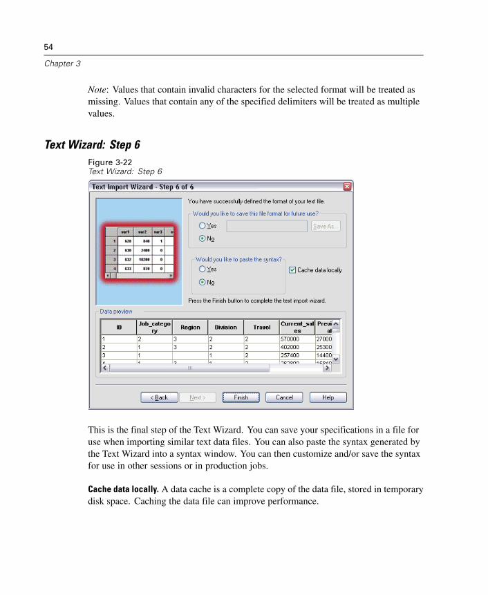
54

Chapter 3

Note: Values that contain invalid characters for the selected format will be treated asmissing. Values that contain any of the specified delimiters will be treated as multiplevalues.


This is the final step of the Text Wizard. You can save your specifications in a file foruse when importing similar text data files. You can also paste the syntax generated bythe Text Wizard into a syntax window. You can then customize and/or save the syntaxfor use in other sessions or in production jobs.

Cache data locally. A data cache is a complete copy of the data file, stored in temporarydisk space. Caching the data file can improve performance.

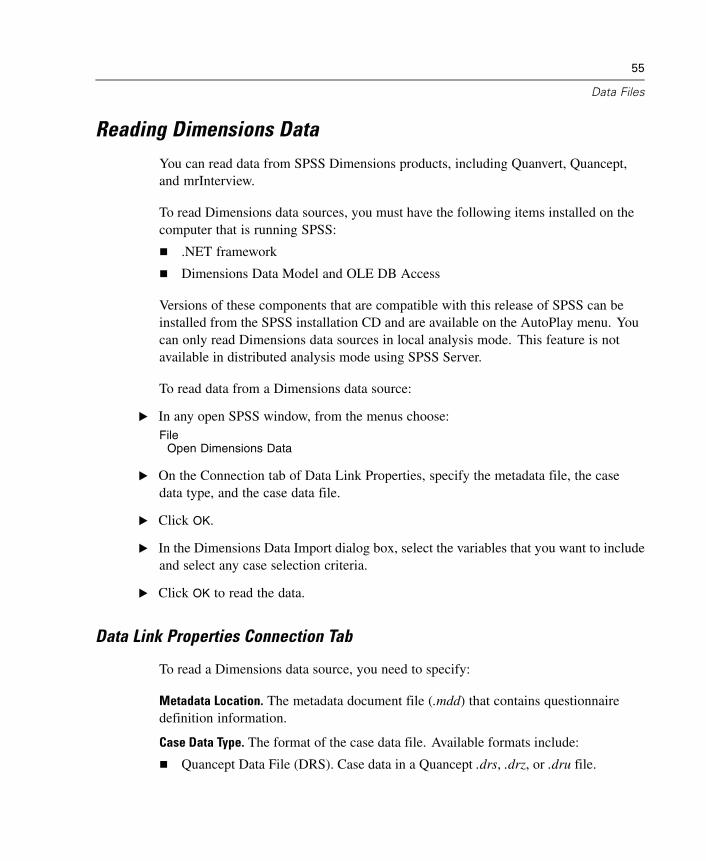
55

Data Files

Reading Dimensions DataYou can read data from SPSS Dimensions products, including Quanvert, Quancept,and mrInterview.

To read Dimensions data sources, you must have the following items installed on thecomputer that is running SPSS:

.NET framework

Dimensions Data Model and OLE DB Access

Versions of these components that are compatible with this release of SPSS can beinstalled from the SPSS installation CD and are available on the AutoPlay menu. Youcan only read Dimensions data sources in local analysis mode. This feature is notavailable in distributed analysis mode using SPSS Server.

To read data from a Dimensions data source:

E In any open SPSS window, from the menus choose:File

Open Dimensions Data

E On the Connection tab of Data Link Properties, specify the metadata file, the casedata type, and the case data file.

E Click OK.

E In the Dimensions Data Import dialog box, select the variables that you want to includeand select any case selection criteria.

E Click OK to read the data.

Data Link Properties Connection Tab

To read a Dimensions data source, you need to specify:

Metadata Location. The metadata document file (.mdd) that contains questionnairedefinition information.

Case Data Type. The format of the case data file. Available formats include:

Quancept Data File (DRS). Case data in a Quancept .drs, .drz, or .dru file.

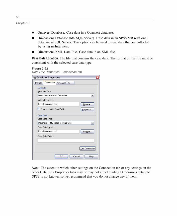
56

Chapter 3

Quanvert Database. Case data in a Quanvert database.

Dimensions Database (MS SQL Server). Case data in an SPSS MR relationaldatabase in SQL Server. This option can be used to read data that are collectedby using mrInterview.

Dimensions XML Data File. Case data in an XML file.

Case Data Location. The file that contains the case data. The format of this file must beconsistent with the selected case data type.

Figure 3-23Data Link Properties: Connection tab

Note: The extent to which other settings on the Connection tab or any settings on theother Data Link Properties tabs may or may not affect reading Dimensions data intoSPSS is not known, so we recommend that you do not change any of them.

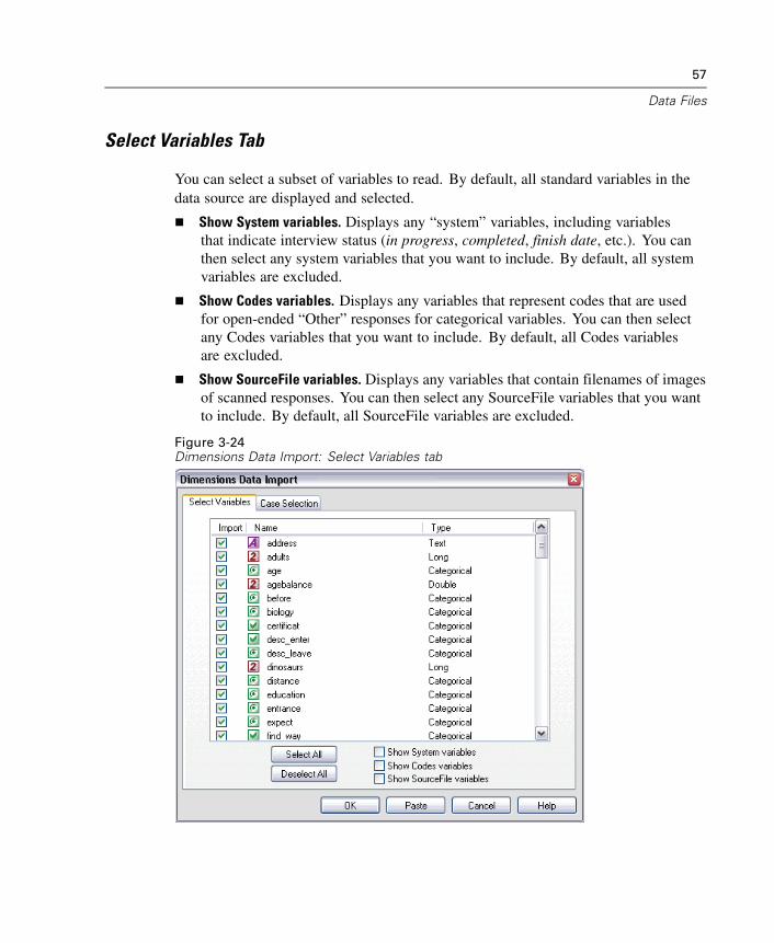
57

Data Files

Select Variables Tab

You can select a subset of variables to read. By default, all standard variables in thedata source are displayed and selected.

Show System variables. Displays any “system” variables, including variablesthat indicate interview status (in progress, completed, finish date, etc.). You canthen select any system variables that you want to include. By default, all systemvariables are excluded.

Show Codes variables. Displays any variables that represent codes that are usedfor open-ended “Other” responses for categorical variables. You can then selectany Codes variables that you want to include. By default, all Codes variablesare excluded.

Show SourceFile variables. Displays any variables that contain filenames of imagesof scanned responses. You can then select any SourceFile variables that you wantto include. By default, all SourceFile variables are excluded.

Figure 3-24Dimensions Data Import: Select Variables tab

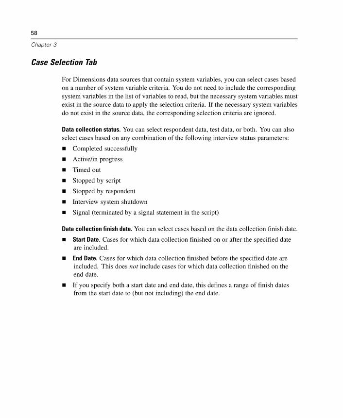
58

Chapter 3

Case Selection Tab

For Dimensions data sources that contain system variables, you can select cases basedon a number of system variable criteria. You do not need to include the correspondingsystem variables in the list of variables to read, but the necessary system variables mustexist in the source data to apply the selection criteria. If the necessary system variablesdo not exist in the source data, the corresponding selection criteria are ignored.

Data collection status. You can select respondent data, test data, or both. You can alsoselect cases based on any combination of the following interview status parameters:

Completed successfully

Active/in progress

Timed out

Stopped by script

Stopped by respondent

Interview system shutdown

Signal (terminated by a signal statement in the script)

Data collection finish date. You can select cases based on the data collection finish date.

Start Date. Cases for which data collection finished on or after the specified dateare included.

End Date. Cases for which data collection finished before the specified date areincluded. This does not include cases for which data collection finished on theend date.

If you specify both a start date and end date, this defines a range of finish datesfrom the start date to (but not including) the end date.

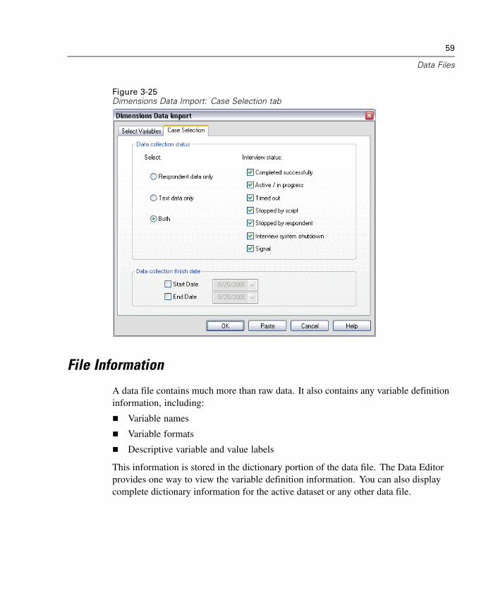
59

Data Files

Figure 3-25Dimensions Data Import: Case Selection tab

File Information

A data file contains much more than raw data. It also contains any variable definitioninformation, including:

Variable names

Variable formats

Descriptive variable and value labels

This information is stored in the dictionary portion of the data file. The Data Editorprovides one way to view the variable definition information. You can also displaycomplete dictionary information for the active dataset or any other data file.

60

Chapter 3

To Obtain Data File Information

E From the menus in the Data Editor window choose:File

Display Data File Information

E For the currently open data file, choose Working File.

E For other data files, choose External File, and then select the data file.

The data file information is displayed in the Viewer.

Saving Data Files

Any changes that you make in a data file last only for the duration of the currentsession—unless you explicitly save the changes.

To Save Modified Data FilesE Make the Data Editor the active window (click anywhere in the window to make

it active).


Save

The modified data file is saved, overwriting the previous version of the file.

Saving Data Files in Excel Format

You can save your data in one of three Microsoft Excel file formats. The choice offormat depends on the version of Excel that will be used to open the data. The Excelapplication cannot open an Excel file from a newer version of the application. Forexample, Excel 5.0 cannot open an Excel 2000 document. However, Excel 2000 caneasily read an Excel 5.0 document.

There are a few limitations to the Excel file format that don’t exist in SPSS. Theselimitations include:

Variable information, such as missing values and variable labels, is not includedin exported Excel files.

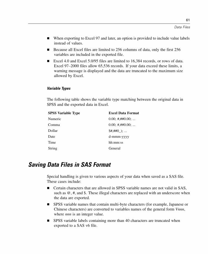
61

Data Files

When exporting to Excel 97 and later, an option is provided to include value labelsinstead of values.

Because all Excel files are limited to 256 columns of data, only the first 256variables are included in the exported file.

Excel 4.0 and Excel 5.0/95 files are limited to 16,384 records, or rows of data.Excel 97–2000 files allow 65,536 records. If your data exceed these limits, awarning message is displayed and the data are truncated to the maximum sizeallowed by Excel.

Variable Types

The following table shows the variable type matching between the original data inSPSS and the exported data in Excel.

SPSS Variable Type Excel Data Format

Numeric 0.00; #,##0.00; ...

Comma 0.00; #,##0.00; ...

Dollar $#,##0_); ...

Date d-mmm-yyyy

Time hh:mm:ss

String General

Saving Data Files in SAS Format

Special handling is given to various aspects of your data when saved as a SAS file.These cases include:

Certain characters that are allowed in SPSS variable names are not valid in SAS,such as @, #, and $. These illegal characters are replaced with an underscore whenthe data are exported.

SPSS variable names that contain multi-byte characters (for example, Japanese orChinese characters) are converted to variables names of the general form Vnnn,where nnn is an integer value.

SPSS variable labels containing more than 40 characters are truncated whenexported to a SAS v6 file.

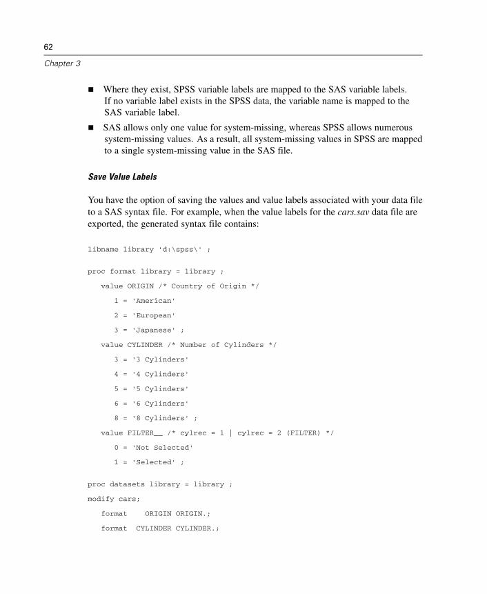
62

Chapter 3

Where they exist, SPSS variable labels are mapped to the SAS variable labels.If no variable label exists in the SPSS data, the variable name is mapped to theSAS variable label.

SAS allows only one value for system-missing, whereas SPSS allows numeroussystem-missing values. As a result, all system-missing values in SPSS are mappedto a single system-missing value in the SAS file.

Save Value Labels

You have the option of saving the values and value labels associated with your data fileto a SAS syntax file. For example, when the value labels for the cars.sav data file areexported, the generated syntax file contains:

libname library 'd:\spss\' ;

proc format library = library ;

value ORIGIN /* Country of Origin */

1 = 'American'

2 = 'European'

3 = 'Japanese' ;

value CYLINDER /* Number of Cylinders */

3 = '3 Cylinders'

4 = '4 Cylinders'

5 = '5 Cylinders'

6 = '6 Cylinders'

8 = '8 Cylinders' ;

value FILTER__ /* cylrec = 1 | cylrec = 2 (FILTER) */

0 = 'Not Selected'

1 = 'Selected' ;

proc datasets library = library ;

modify cars;

format ORIGIN ORIGIN.;

format CYLINDER CYLINDER.;

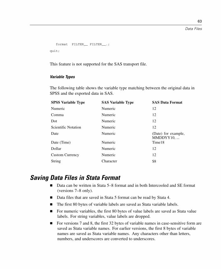
63

Data Files

format FILTER__ FILTER__.;

quit;

This feature is not supported for the SAS transport file.

Variable Types

The following table shows the variable type matching between the original data inSPSS and the exported data in SAS.

SPSS Variable Type SAS Variable Type SAS Data Format

Numeric Numeric 12

Comma Numeric 12

Dot Numeric 12

Scientific Notation Numeric 12

Date Numeric (Date) for example,MMDDYY10, ...

Date (Time) Numeric Time18

Dollar Numeric 12

Custom Currency Numeric 12

String Character $8

Saving Data Files in Stata FormatData can be written in Stata 5–8 format and in both Intercooled and SE format(versions 7–8 only).

Data files that are saved in Stata 5 format can be read by Stata 4.

The first 80 bytes of variable labels are saved as Stata variable labels.

For numeric variables, the first 80 bytes of value labels are saved as Stata valuelabels. For string variables, value labels are dropped.

For versions 7 and 8, the first 32 bytes of variable names in case-sensitive form aresaved as Stata variable names. For earlier versions, the first 8 bytes of variablenames are saved as Stata variable names. Any characters other than letters,numbers, and underscores are converted to underscores.

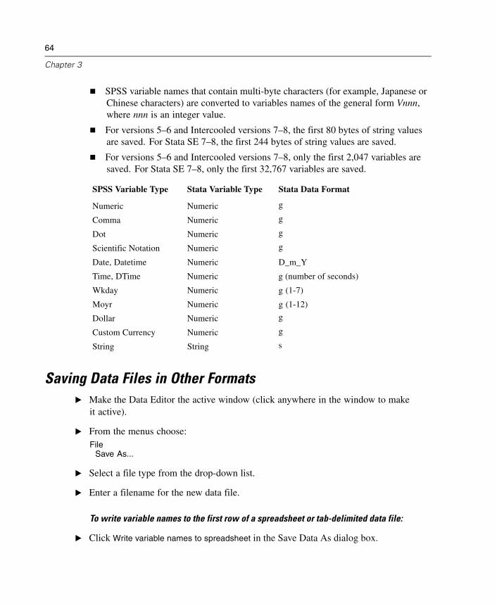
64

Chapter 3

SPSS variable names that contain multi-byte characters (for example, Japanese orChinese characters) are converted to variables names of the general form Vnnn,where nnn is an integer value.

For versions 5–6 and Intercooled versions 7–8, the first 80 bytes of string valuesare saved. For Stata SE 7–8, the first 244 bytes of string values are saved.

For versions 5–6 and Intercooled versions 7–8, only the first 2,047 variables aresaved. For Stata SE 7–8, only the first 32,767 variables are saved.

SPSS Variable Type Stata Variable Type Stata Data Format

Numeric Numeric g

Comma Numeric g

Dot Numeric g

Scientific Notation Numeric g

Date, Datetime Numeric D_m_Y

Time, DTime Numeric g (number of seconds)

Wkday Numeric g (1-7)

Moyr Numeric g (1-12)

Dollar Numeric g

Custom Currency Numeric g

String String s

Saving Data Files in Other FormatsE Make the Data Editor the active window (click anywhere in the window to make

it active).


Save As...

E Select a file type from the drop-down list.

E Enter a filename for the new data file.

To write variable names to the first row of a spreadsheet or tab-delimited data file:

E Click Write variable names to spreadsheet in the Save Data As dialog box.

65

Data Files

To save value labels instead of data values in Excel 97 format:

E Click Save value labels where defined instead of data values in the Save Data As dialogbox.

To save value labels to a SAS syntax file (active only when a SAS file type is selected):

E Click Save value labels into a .sas file in the Save Data As dialog box.

Saving Data: Data File Types

You can save data in the following formats:

SPSS (*.sav). SPSS format.

Data files saved in SPSS format cannot be read by versions of the software priorto version 7.5.

When using data files with variable names longer than eight bytes in SPSS 10.xor 11.x, unique, eight-byte versions of variable names are used—but the originalvariable names are preserved for use in release 12.0 or later. In releases prior toSPSS 10.0, the original long variable names are lost if you save the data file.

When using data files with string variables longer than 255 bytes in versions ofSPSS prior to release 13.0, those string variables are broken up into multiple255-byte string variables.

SPSS 7.0 (*.sav). SPSS 7.0 for Windows format. Data files saved in SPSS 7.0 formatcan be read by SPSS 7.0 and earlier versions of SPSS for Windows but do not includedefined multiple response sets or Data Entry for Windows information.

SPSS/PC+ (*.sys). SPSS/PC+ format. If the data file contains more than 500 variables,only the first 500 will be saved. For variables with more than one defined user-missingvalue, additional user-missing values will be recoded into the first defined user-missingvalue.

SPSS Portable (*.por). SPSS portable format that can be read by other versions of SPSSand versions on other operating systems (for example, Macintosh or UNIX). Variablenames are limited to eight bytes and are automatically converted to unique eight-bytenames if necessary.

Tab-delimited (*.dat). ASCII text files with values separated by tabs.

66

Chapter 3

Fixed ASCII (*.dat). ASCII text file in fixed format, using the default write formats forall variables. There are no tabs or spaces between variable fields.

Excel 2.1 (*.xls). Microsoft Excel 2.1 spreadsheet file. The maximum number ofvariables is 256, and the maximum number of rows is 16,384.

Excel 97 and later (*.xls). Microsoft Excel 97/2000/XP spreadsheet file. The maximumnumber of variables is 256, and the maximum number of rows is 65,536.

1-2-3 Release 3.0 (*.wk3). Lotus 1-2-3 spreadsheet file, release 3.0. The maximumnumber of variables that you can save is 256.

1-2-3 Release 2.0 (*.wk1). Lotus 1-2-3 spreadsheet file, release 2.0. The maximumnumber of variables that you can save is 256.

1-2-3 Release 1.0 (*.wks). Lotus 1-2-3 spreadsheet file, release 1A. The maximumnumber of variables that you can save is 256.

SYLK (*.slk). Symbolic link format for Microsoft Excel and Multiplan spreadsheet files.The maximum number of variables that you can save is 256.

dBASE IV (*.dbf). dBASE IV format.

dBASE III (*.dbf). dBASE III format.

dBASE II (*.dbf). dBASE II format.

SAS v6 for Windows (*.sd2). SAS v6 file format for Windows/OS2.

SAS v6 for UNIX (*.ssd01). SAS v6 file format for UNIX (Sun, HP, IBM).

SAS v6 for Alpha/OSF (*.ssd04). SAS v6 file format for Alpha/OSF (DEC UNIX).

SAS v7+ Windows short extension (*.sd7). SAS versions 7–8 for Windows short filenameformat.

SAS v7+ Windows long extension (*.sas7bdat). SAS versions 7–8 for Windows longfilename format.

SAS v7+ for UNIX (*.ssd01). SAS v8 for UNIX.

SAS Transport (*.xpt). SAS transport file.

Stata Versions 4–5 (*.dta).

Stata Version 6 (*.dta).

Stata Version 7 Intercooled (*.dta).

Stata Version 7 SE (*.dta).

67

Data Files

Stata Version 8 Intercooled (*.dta).

Stata Version 8 SE (*.dta).

Saving Subsets of VariablesFigure 3-26Save Data As Variables dialog box

The Save Data As Variables dialog box allows you to select the variables that you wantto be saved in the new data file. By default, all variables will be saved. Deselect thevariables that you don’t want to save, or click Drop All and then select the variables thatyou want to save.

To Save a Subset of Variables

E Make the Data Editor the active window (click anywhere in the window to makeit active).


Save As...

E Select the file types the file type.

E Click Variables.

68

Chapter 3

E Select the variables that you want to save.

Saving File Options

For spreadsheet and tab-delimited files, you can write variable names to the first rowof the file.

Protecting Original Data

To prevent the accidental modification/deletion of your original data, you can markthe file as read-only.

E From the Data Editor menus choose:File

Mark File Read Only

If you make subsequent modifications to the data and then try to save the data file, youcan save the data only with a different filename, so the original data are not affected.

You can change the file permissions back to read/write by selecting Mark File Read

Write from the File menu.

Virtual Active File

The virtual active file enables you to work with large data files without requiringequally large (or larger) amounts of temporary disk space. For most analysis andcharting procedures, the original data source is reread each time you run a differentprocedure. Procedures that modify the data require a certain amount of temporary diskspace to keep track of the changes, and some actions always require enough disk spacefor at least one entire copy of the data file.

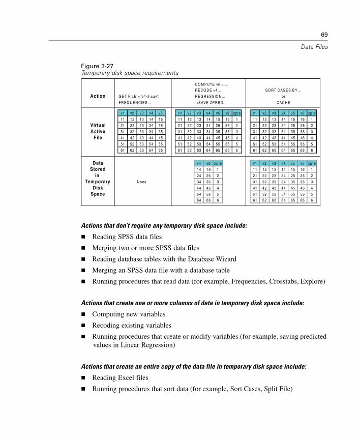
69

Data Files

Figure 3-27Temporary disk space requirements

C O M P U TE v6 = …

R E C O D E v4…

Action G ET FILE = 'v1-5 .sav'. R EG R ES SIO N … or

FR E Q U E N C IE S … /S AV E ZP R E D.

v1 v2 v3 v4 v5 v1 v2 v3 v4 v5 v6 zpre v1 v2 v3 v4 v5 v6 zpre

11 12 13 14 15 11 12 13 14 15 16 1 11 12 13 14 15 16 1

Virtual 21 22 23 24 25 21 22 23 24 25 26 2 21 22 23 24 25 26 2

Active 31 32 33 34 35 31 32 33 34 35 36 3 31 32 33 34 35 36 3

File 41 42 43 44 45 41 42 43 44 45 46 4 41 42 43 44 45 46 4

51 52 53 54 55 51 52 53 54 55 56 5 51 52 53 54 55 56 5

61 62 63 64 65 61 62 63 64 65 66 6 61 62 63 64 65 66 6

Data v4 v6 zpre v1 v2 v3 v4 v5 v6 zpre

Stored 14 16 1 11 12 13 14 15 16 1

in 24 26 2 21 22 23 24 25 26 2

Tem porary 34 36 3 31 32 33 34 35 36 3

Disk 44 46 4 41 42 43 44 45 46 4

Space 54 56 5 51 52 53 54 55 56 5

64 66 6 61 62 63 64 65 66 6

C AC H E

S O RT C A S E S B Y …

N one

Actions that don’t require any temporary disk space include:

Reading SPSS data files

Merging two or more SPSS data files

Reading database tables with the Database Wizard

Merging an SPSS data file with a database table

Running procedures that read data (for example, Frequencies, Crosstabs, Explore)

Actions that create one or more columns of data in temporary disk space include:

Computing new variables

Recoding existing variables

Running procedures that create or modify variables (for example, saving predictedvalues in Linear Regression)

Actions that create an entire copy of the data file in temporary disk space include:

Reading Excel files

Running procedures that sort data (for example, Sort Cases, Split File)

70

Chapter 3

Reading data with GET TRANSLATE or DATA LIST commands

Using the Cache Data facility or the CACHE command

Launching other applications from SPSS that read the data file (for example,AnswerTree, DecisionTime)

Note: The GET DATA command provides functionality comparable to DATA LIST

without creating an entire copy of the data file in temporary disk space. The SPLITFILE command in command syntax does not sort the data file and therefore doesnot create a copy of the data file. This command, however, requires sorted data forproper operation, and the dialog box interface for this procedure will automaticallysort the data file, resulting in a complete copy of the data file. (Command syntax isnot available with the Student Version.)

Actions that create an entire copy of the data file by default:

Reading databases with the Database Wizard

Reading text files with the Text Wizard

The Text Wizard provide an optional setting to automatically cache the data. Bydefault, this option is selected. You can turn it off by deselecting Cache data locally.For the Database Wizard you can paste the generated command syntax and delete theCACHE command.

Creating a Data Cache

Although the virtual active file can vastly reduce the amount of temporary disk spacerequired, the absence of a temporary copy of the “active” file means that the originaldata source has to be reread for each procedure. For large data files read from anexternal source, creating a temporary copy of the data may improve performance. Forexample, for data tables read from a database source, the SQL query that reads theinformation from the database must be reexecuted for any command or procedure thatneeds to read the data. Since virtually all statistical analysis procedures and chartingprocedures need to read the data, the SQL query is reexecuted for each procedure yourun, which can result in a significant increase in processing time if you run a largenumber of procedures.

71

Data Files

If you have sufficient disk space on the computer performing the analysis (eitheryour local computer or a remote server), you can eliminate multiple SQL queries andimprove processing time by creating a data cache of the active file. The data cache isa temporary copy of the complete data.

Note: By default, the Database Wizard automatically creates a data cache, but if youuse the GET DATA command in command syntax to read a database, a data cache is notautomatically created. (Command syntax is not available with the Student Version.)

To Create a Data Cache


Cache Data...

E Click OK or Cache Now.

OK creates a data cache the next time the program reads the data (for example, thenext time you run a statistical procedure), which is usually what you want because itdoesn’t require an extra data pass. Cache Now creates a data cache immediately, whichshouldn’t be necessary under most circumstances. Cache Now is useful primarily fortwo reasons:

A data source is “locked” and can’t be updated by anyone until you end yoursession, open a different data source, or cache the data.

For large data sources, scrolling through the contents of the Data View tab in theData Editor will be much faster if you cache the data.

To Cache Data Automatically

You can use the SET command to automatically create a data cache after a specifiednumber of changes in the active data file. By default, the active data file isautomatically cached after 20 changes in the active data file.


NewSyntax

E In the syntax window, type SET CACHE n. (where n represents the number of changesin the active data file before the data file is cached).

72

Chapter 3

E From the menus in the syntax window choose:Run

All

Note: The cache setting is not persistent across sessions. Each time you start a newsession, the value is reset to the default of 20.

Chapter

4Distributed Analysis Mode

Distributed analysis mode allows you to use a computer other than your local (ordesktop) computer for memory-intensive work. Because remote servers that areused for distributed analysis are typically more powerful and faster than your localcomputer, distributed analysis mode can significantly reduce computer processingtime. Distributed analysis with a remote server can be useful if your work involves:

Large data files, particularly data that are read from database sources.

Memory-intensive tasks. Any task that takes a long time in local analysis modemight be a good candidate for distributed analysis.

Distributed analysis affects only data-related tasks, such as reading data, transformingdata, computing new variables, and calculating statistics. Distributed analysis has noeffect on tasks that are related to editing output, such as manipulating pivot tables ormodifying charts.

Note: Distributed analysis is available only if you have both a local version and accessto a licensed server version of the software that is installed on a remote server.

Distributed Analysis versus Local Analysis

Following are some guidelines for choosing distributed analysis or local analysis mode:

Database access. Jobs that perform database queries may run faster in distributed modeif the server has superior access to the database or if the server is running on the samemachine as the database engine. Additionally, if the necessary database-access softwareis available only on the server, or if your network administrator does not permit you todownload large data tables, you can access the database only in distributed mode.

Ratio of computation to output. Commands that have the most to gain from running indistributed mode are commands that perform a lot of computation and produce smalloutput results (for example, few and small pivot tables, brief text results, or few and

73

74

Chapter 4

simple charts). The degree of improvement depends largely on the computing power ofthe remote server.

Small jobs. Jobs that run quickly in local mode will almost always run slower indistributed mode because of inherent client/server overhead.

Charts. Case-oriented charts, such as scatterplots, regression residual plots, andsequence charts, require raw data on your local computer. For large data files ordatabase tables, this process can result in slower performance in distributed modebecause the data have to be sent from the remote server to your local computer. Othercharts are based on summarized or aggregated data and should perform adequatelybecause the aggregation is performed on the server.

Interactive graphics. If raw data is saved with interactive graphics (an optional setting),large amounts of data may be transferred from the remote server to your localcomputer, significantly increasing the time that it takes to save your results.

Pivot tables. Large pivot tables may take longer to create in distributed mode. Thissituation is particularly true for the OLAP Cubes procedure and tables that containindividual case data, such as those tables that are available in the Summarize procedure.

Text output. The more text that is produced, the slower output will be in distributed modebecause the text is produced on the remote server and copied to your local computerfor display. Text results have low overhead, however, and tend to transmit quickly.

Server Login

The Server Login dialog box allows you to select the computer that processescommands and runs procedures. You can select your local computer or a remote server.

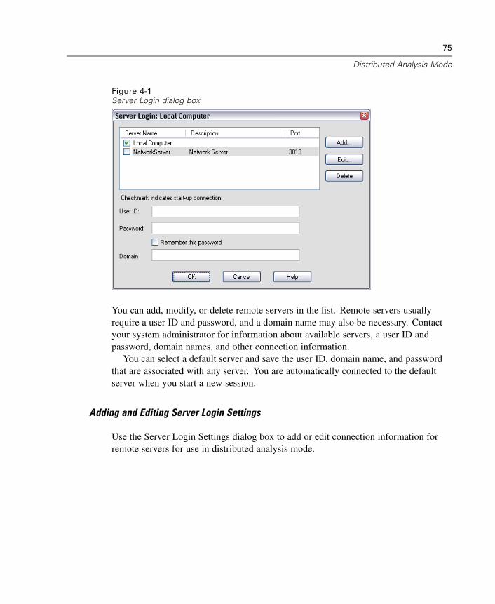
75

Distributed Analysis Mode

Figure 4-1Server Login dialog box

You can add, modify, or delete remote servers in the list. Remote servers usuallyrequire a user ID and password, and a domain name may also be necessary. Contactyour system administrator for information about available servers, a user ID andpassword, domain names, and other connection information.

You can select a default server and save the user ID, domain name, and passwordthat are associated with any server. You are automatically connected to the defaultserver when you start a new session.

Adding and Editing Server Login Settings

Use the Server Login Settings dialog box to add or edit connection information forremote servers for use in distributed analysis mode.

76

Chapter 4

Figure 4-2Server Login Settings dialog box

Contact your system administrator for a list of available servers, port numbers for theservers, and additional connection information. Do not use the Secure Socket Layerunless instructed to do so by your administrator.

Server Name. A server “name” can be an alphanumeric name that is assigned to acomputer (for example, NetworkServer) or a unique IP address that is assigned to acomputer (for example, 202.123.456.78).

Port Number. The port number is the port that the server software uses forcommunications.

Description. You can enter an optional description to display in the servers list.

Connect with Secure Socket Layer. Secure Socket Layer (SSL) encrypts requests fordistributed analysis when they are sent to the remote SPSS server. Before you use SSL,check with your administrator. For this option to be enabled, SSL must be configuredon your desktop computer and the server.

To Select, Switch, or Add Servers


Switch Server...

To select a default server:

E In the server list, select the box next to the server that you want to use.

77


E Enter the user ID, domain name, and password that were provided by youradministrator.

Note: You are automatically connected to the default server when you start a newsession.

To switch to another server:

E Select the server from the list.

E Enter your user ID, domain name, and password (if necessary).

Note: When you switch servers during a session, all open windows are closed. Youwill be prompted to save changes before the windows are closed.

To add a server:

E Get the server connection information from your administrator.

E Click Add to open the Server Login Settings dialog box.

E Enter the connection information and optional settings, and then click OK.

To edit a server:

E Get the revised connection information from your administrator.

E Click Edit to open the Server Login Settings dialog box.

E Enter the changes and click OK.

78

Chapter 4

Opening Data Files from a Remote ServerFigure 4-3Open Remote File dialog box

In distributed analysis mode, the Open Remote File dialog box replaces the standardOpen File dialog box.

The contents of the list of available files, folders, and drives depends on what isavailable on or from the remote server. The current server name is indicated at thetop of the dialog box.

In distributed analysis mode, you will not have access to files on your localcomputer unless you specify the drive as a shared device or the specify the folderscontaining your data files as shared folders.

If the server is running a different operating system (for example, you are runningWindows and the server is running UNIX), you probably won’t have access tolocal data files in distributed analysis mode even if they are in shared folders.

To Open Data Files from a Remote Server

E If you aren’t already connected to the remote server, log in to the remote server.

E Depending on the type of data file that you want to open, from the menus choose:File

OpenData...

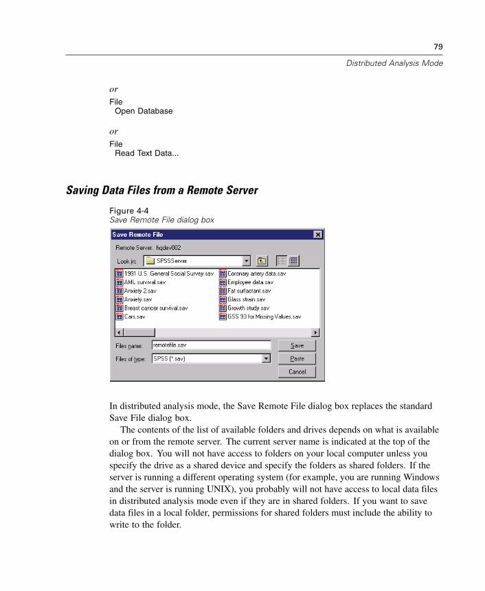
79


orFile

Open Database

orFile

Read Text Data...

Saving Data Files from a Remote Server

Figure 4-4Save Remote File dialog box

In distributed analysis mode, the Save Remote File dialog box replaces the standardSave File dialog box.

The contents of the list of available folders and drives depends on what is availableon or from the remote server. The current server name is indicated at the top of thedialog box. You will not have access to folders on your local computer unless youspecify the drive as a shared device and specify the folders as shared folders. If theserver is running a different operating system (for example, you are running Windowsand the server is running UNIX), you probably will not have access to local data filesin distributed analysis mode even if they are in shared folders. If you want to savedata files in a local folder, permissions for shared folders must include the ability towrite to the folder.

80

Chapter 4

To Save Data Files from a Remote Server

E Make the Data Editor the active window.


Save (or Save As...)

Data File Access in Local and Distributed Analysis Mode

The view of data files, folders (directories), and drives for both your local computerand the network is based on the computer that you are currently using to processcommands and run procedures—which is not necessarily the computer in front of you.

Local analysis mode. When you use your local computer as your “server,” the view ofdata files, folders, and drives in the file access dialog box (for opening data files) issimilar to what you see in other applications or in Windows Explorer. You can see allof the data files and folders on your computer and any files and folders on mountednetwork drives.

Distributed analysis mode. When you use another computer as a “remote server” to runcommands and procedures, the view of data files, folders, and drives represents theview from the remote server computer. Although you may see familiar folder names(such as Program Files) and drives (such as C), these items are not the folders anddrives on your computer; they are the folders and drives on the remote server.

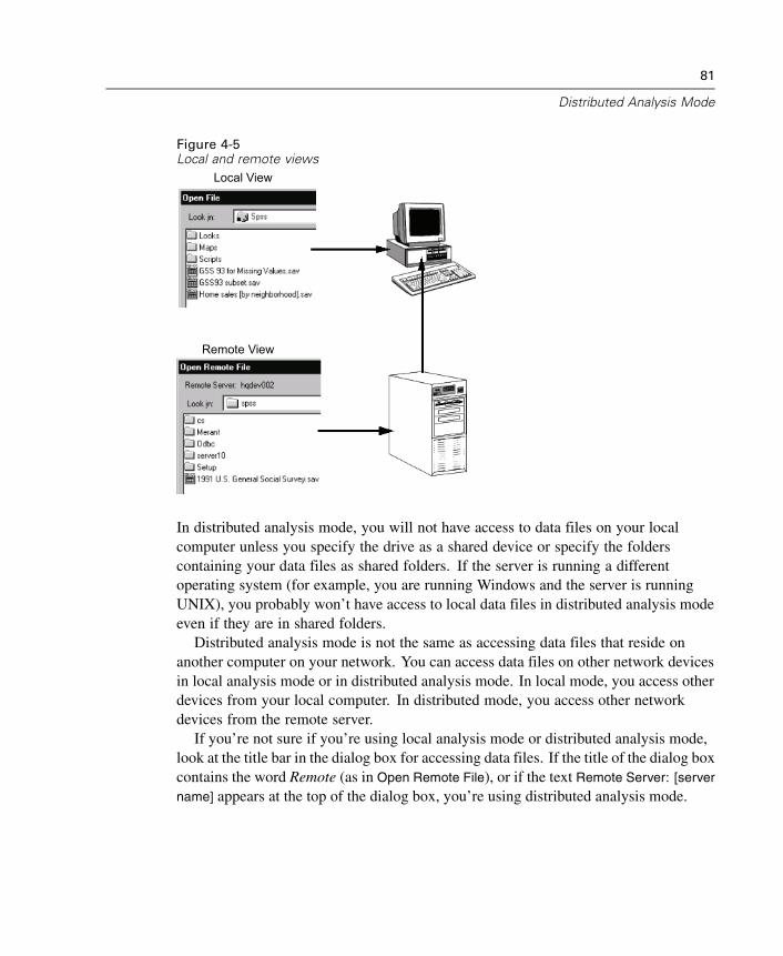
81


Figure 4-5Local and remote views

Local View

Remote View

In distributed analysis mode, you will not have access to data files on your localcomputer unless you specify the drive as a shared device or specify the folderscontaining your data files as shared folders. If the server is running a differentoperating system (for example, you are running Windows and the server is runningUNIX), you probably won’t have access to local data files in distributed analysis modeeven if they are in shared folders.

Distributed analysis mode is not the same as accessing data files that reside onanother computer on your network. You can access data files on other network devicesin local analysis mode or in distributed analysis mode. In local mode, you access otherdevices from your local computer. In distributed mode, you access other networkdevices from the remote server.

If you’re not sure if you’re using local analysis mode or distributed analysis mode,look at the title bar in the dialog box for accessing data files. If the title of the dialog boxcontains the word Remote (as in Open Remote File), or if the text Remote Server: [server

name] appears at the top of the dialog box, you’re using distributed analysis mode.

82

Chapter 4

Note: This situation affects only dialog boxes for accessing data files (for example,Open Data, Save Data, Open Database, and Apply Data Dictionary). For all otherfile types (for example, Viewer files, syntax files, and script files), the local view isalways used.

To Set Sharing Permissions for a Drive or Folder

E In My Computer, click the folder (directory) or drive that you want to share.

E From the File menu, choose Properties.

E Click the Sharing tab, and then click Shared As.

For more information about sharing drives and folders, see the Help for your operatingsystem.

Availability of Procedures in Distributed Analysis Mode

In distributed analysis mode, procedures are available for use only if they are installedon both your local version and the version on the remote server.

If you have optional components installed locally that are not available on theremote server, and you switch from your local computer to a remote server, the affectedprocedures will be removed from the menus, and the corresponding command syntaxwill result in errors. Switching back to local mode will restore all affected procedures.

Using UNC Path Specifications

With the Windows NT server version of SPSS, relative path specifications for data filesare relative to the current server in distributed analysis mode, not relative to yourlocal computer. A path specification (such as c:\mydocs\mydata.sav) does not pointto a directory and file on your C drive; it points to a directory and file on the remoteserver’s hard drive. If the directory and/or file do not exist on the remote server, anerror results in command syntax, as in the following example:

GET FILE='c:\mydocs\mydata.sav'.

83


If you are using the Windows NT server version of SPSS, you can use universalnaming convention (UNC) specifications when accessing data files with commandsyntax. The general form of a UNC specification is:

\\servername\sharename\path\filename

Servername is the name of the computer that contains the data file.

Sharename is the folder (directory) on that computer that is designated as a sharedfolder.

Path is any additional folder (subdirectory) path below the shared folder.

Filename is the name of the data file.

An example is as follows:

GET FILE='\\hqdev001\public\july\sales.sav'.

If the computer does not have a name assigned to it, you can use its IP address, as in:

GET FILE='\\204.125.125.53\public\july\sales.sav'.

Even with UNC path specifications, you can access data files only from devices andfolders that are designated as shared. When you use distributed analysis mode, thissituation includes data files on your local computer.

UNIX servers. On UNIX platforms, there is no equivalent to the UNC path, and alldirectory paths must be absolute paths that start at the root of the server; relativepaths are not allowed. For example, if the data file is located in /bin/spss/data andthe current directory is also /bin/spss/data, GET FILE='sales.sav' is not valid;you must specify the entire path, as in:

GET FILE='/bin/spss/data/sales.sav'.

Chapter

5Data Editor

The Data Editor provides a convenient, spreadsheet-like method for creating andediting data files. The Data Editor window opens automatically when you start asession.

The Data Editor provides two views of your data:

Data View. This view displays the actual data values or defined value labels.

Variable View. This view displays variable definition information, including definedvariable and value labels, data type (for example, string, date, and numeric),measurement level (nominal, ordinal, or scale), and user-defined missing values.

In both views, you can add, change, and delete information that is contained in thedata file.

85

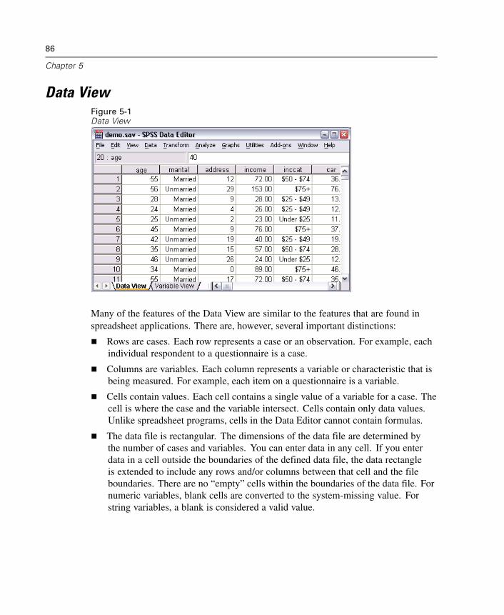
86

Chapter 5

Data ViewFigure 5-1Data View

Many of the features of the Data View are similar to the features that are found inspreadsheet applications. There are, however, several important distinctions:

Rows are cases. Each row represents a case or an observation. For example, eachindividual respondent to a questionnaire is a case.

Columns are variables. Each column represents a variable or characteristic that isbeing measured. For example, each item on a questionnaire is a variable.

Cells contain values. Each cell contains a single value of a variable for a case. Thecell is where the case and the variable intersect. Cells contain only data values.Unlike spreadsheet programs, cells in the Data Editor cannot contain formulas.

The data file is rectangular. The dimensions of the data file are determined bythe number of cases and variables. You can enter data in any cell. If you enterdata in a cell outside the boundaries of the defined data file, the data rectangleis extended to include any rows and/or columns between that cell and the fileboundaries. There are no “empty” cells within the boundaries of the data file. Fornumeric variables, blank cells are converted to the system-missing value. Forstring variables, a blank is considered a valid value.

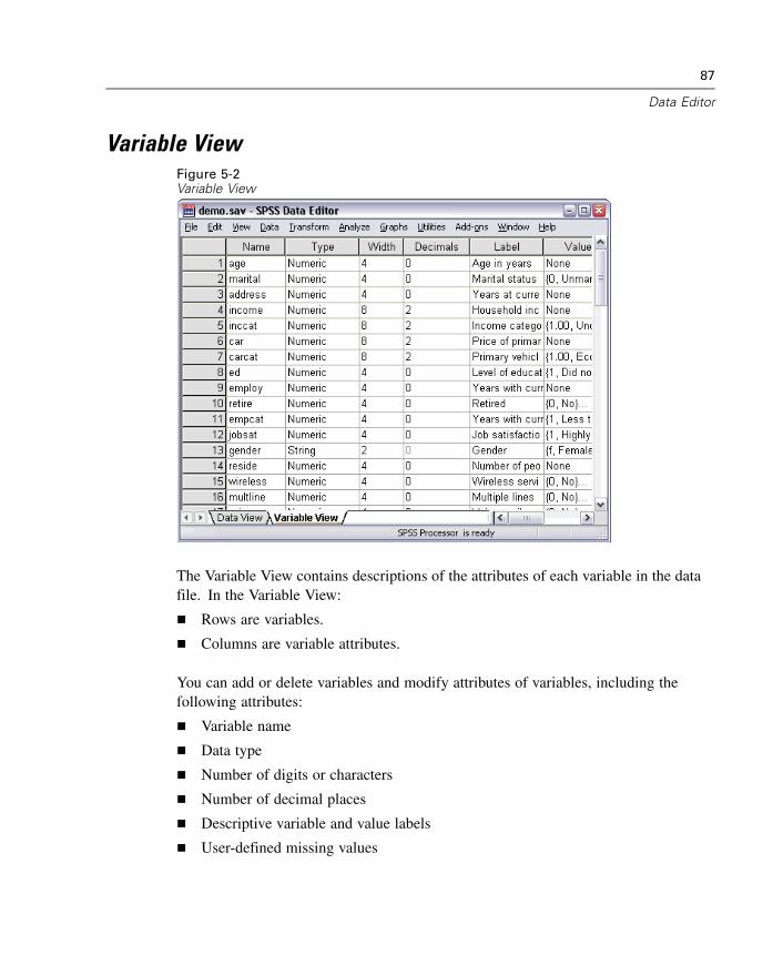
87

Data Editor

Variable ViewFigure 5-2Variable View

The Variable View contains descriptions of the attributes of each variable in the datafile. In the Variable View:

Rows are variables.

Columns are variable attributes.

You can add or delete variables and modify attributes of variables, including thefollowing attributes:

Variable name

Data type

Number of digits or characters

Number of decimal places

Descriptive variable and value labels

User-defined missing values

88

Chapter 5

Column width

Measurement level

All of these attributes are saved when you save the data file.

In addition to defining variable properties in the Variable View, there are two othermethods for defining variable properties:

The Copy Data Properties Wizard provides the ability to use an external SPSSdata file or another dataset that is available in the current session as a templatefor defining file and variable properties in the active dataset. You can also usevariables in the active dataset as templates for other variables in the active dataset.Copy Data Properties is available on the Data menu in the Data Editor window.

Define Variable Properties (also available on the Data menu in the Data Editorwindow) scans your data and lists all unique data values for any selected variables,identifies unlabeled values, and provides an auto-label feature. This method isparticularly useful for categorical variables that use numeric codes to representcategories—for example, 0 = Male, 1 = Female.

To Display or Define Variable Attributes


E Double-click a variable name at the top of the column in the Data View, or click theVariable View tab.

E To define new variables, enter a variable name in any blank row.

E Select the attribute(s) that you want to define or modify.

Variable Names

The following rules apply to variable names:

The name must begin with a letter. The remaining characters can be any letter, anydigit, a period, or the symbols @, #, _, or $.

Variable names cannot end with a period.

Ending variable names with an underscore should be avoided (to avoid conflictwith variables that are automatically created by some procedures).

89

Data Editor

The length of the name cannot exceed 64 bytes. Typically, 64 bytes means 64characters in single-byte languages (for example, English, French, German,Spanish, Italian, Hebrew, Russian, Greek, Arabic, Thai), and it typically means 32characters in double-byte languages (for example, Japanese, Chinese, Korean).

Blanks and special characters (for example, !, ?, ‘, and *) cannot be used.

Each variable name must be unique; duplication is not allowed.

Reserved keywords cannot be used as variable names. Reserved keywords are:ALL, AND, BY, EQ, GE, GT, LE, LT, NE, NOT, OR, TO, WITH.

Variable names can be defined with any mixture of uppercase and lowercasecharacters, and case is preserved for display purposes.

When long variable names need to wrap onto multiple lines in output, SPSSattempts to break the lines at underscores, periods, and where content changesfrom lowercase to uppercase.

Variable Measurement Level

You can specify the level of measurement as scale (numeric data on an intervalor ratio scale), ordinal, or nominal. Nominal and ordinal data can be either string(alphanumeric) or numeric.

Nominal. A variable can be treated as nominal when its values represent categorieswith no intrinsic ranking; for example, the department of the company in whichan employee works. Examples of nominal variables include region, zip code,or religious affiliation.

Ordinal. A variable can be treated as ordinal when its values represent categorieswith some intrinsic ranking; for example, levels of service satisfaction fromhighly dissatisfied to highly satisfied. Examples of ordinal variables includeattitude scores representing degree of satisfaction or confidence and preferencerating scores.

Scale. A variable can be treated as scale when its values represent orderedcategories with a meaningful metric, so that distance comparisons between valuesare appropriate. Examples of scale variables include age in years and incomein thousands of dollars.

Note: For ordinal string variables, the alphabetic order of string values is assumed toreflect the true order of the categories. For example, for a string variable with thevalues of low, medium, high, the order of the categories is interpreted as high, low,

90

Chapter 5

medium—which is not the correct order. In general, it is more reliable to use numericcodes to represent ordinal data.

For new variables created during a session, data read from external file formats, andSPSS data files that were created prior to version 8, default assignment of measurementlevel is based on the following rules:

Numeric variables with fewer than 24 unique values and string variables are set tonominal.

Numeric variables with 24 or more unique values are set to scale.

You can change the scale/nominal cutoff value for numeric variables in the Optionsdialog box. For more information, see “Interactive Chart Options” in Chapter 44on p. 607.

The Define Variable Properties dialog box, available from the Data menu, can helpyou assign the correct measurement level. For more information, see “Assigning theMeasurement Level” in Chapter 7 on p. 116.

Variable Type

Variable Type specifies the data type for each variable. By default, all new variablesare assumed to be numeric. You can use Variable Type to change the data type. Thecontents of the Variable Type dialog box depend on the selected data type. For somedata types, there are text boxes for width and number of decimals; for other data types,you can simply select a format from a scrollable list of examples.

Figure 5-3Variable Type dialog box

91

Data Editor

The available data types are as follows:

Numeric. A variable whose values are numbers. Values are displayed in standardnumeric format. The Data Editor accepts numeric values in standard format or inscientific notation.

Comma. A numeric variable whose values are displayed with commas delimiting everythree places and displayed with the period as a decimal delimiter. The Data Editoraccepts numeric values for comma variables with or without commas or in scientificnotation. Values cannot contain commas to the right of the decimal indicator.

Dot. A numeric variable whose values are displayed with periods delimiting every threeplaces and with the comma as a decimal delimiter. The Data Editor accepts numericvalues for dot variables with or without periods or in scientific notation. Values cannotcontain periods to the right of the decimal indicator.

Scientific notation. A numeric variable whose values are displayed with an embeddedE and a signed power-of-ten exponent. The Data Editor accepts numeric values forsuch variables with or without an exponent. The exponent can be preceded by E orD with an optional sign or by the sign alone—for example, 123, 1.23E2, 1.23D2,1.23E+2, and 1.23+2.

Date. A numeric variable whose values are displayed in one of several calendar-date orclock-time formats. Select a format from the list. You can enter dates with slashes,hyphens, periods, commas, or blank spaces as delimiters. The century range fortwo-digit year values is determined by your Options settings (from the Edit menu,choose Options, and then click the Data tab).

Dollar. A numeric variable displayed with a leading dollar sign ($), commas delimitingevery three places, and a period as the decimal delimiter. You can enter data valueswith or without the leading dollar sign.

Custom currency. A numeric variable whose values are displayed in one of the customcurrency formats that you have defined in the Currency tab of the Options dialog box.Defined custom currency characters cannot be used in data entry but are displayedin the Data Editor.

String. A variable whose values are not numeric and therefore are not used incalculations. The values can contain any characters up to the defined length.Uppercase and lowercase letters are considered distinct. This type is also known as analphanumeric variable.

92

Chapter 5

To Define Variable Type

E Click the button in the Type cell for the variable that you want to define.

E Select the data type in the Variable Type dialog box.

E Click OK.

Input versus Display Formats

Depending on the format, the display of values in the Data View may differ from theactual value as entered and stored internally. Following are some general guidelines:

For numeric, comma, and dot formats, you can enter values with any number ofdecimal positions (up to 16), and the entire value is stored internally. The DataView displays only the defined number of decimal places and rounds values withmore decimals. However, the complete value is used in all computations.

For string variables, all values are right-padded to the maximum width. For astring variable with a maximum width of three, a value of No is stored internally as'No ' and is not equivalent to ' No'.

For date formats, you can use slashes, dashes, spaces, commas, or periods asdelimiters between day, month, and year values, and you can enter numbers,three-letter abbreviations, or complete names for month values. Dates of thegeneral format dd-mmm-yy are displayed with dashes as delimiters and three-letterabbreviations for the month. Dates of the general format dd/mm/yy and mm/dd/yyare displayed with slashes for delimiters and numbers for the month. Internally,dates are stored as the number of seconds from October 14, 1582. The centuryrange for dates with two-digit years is determined by your Options settings (fromthe Edit menu, choose Options, and then click the Data tab).

For time formats, you can use colons, periods, or spaces as delimiters betweenhours, minutes, and seconds. Times are displayed with colons as delimiters.Internally, times are stored as the number of seconds from October 14, 1582.

Variable Labels

You can assign descriptive variable labels up to 256 characters (128 characters indouble-byte languages). Variable labels can contain spaces and reserved charactersthat are not allowed in variable names.

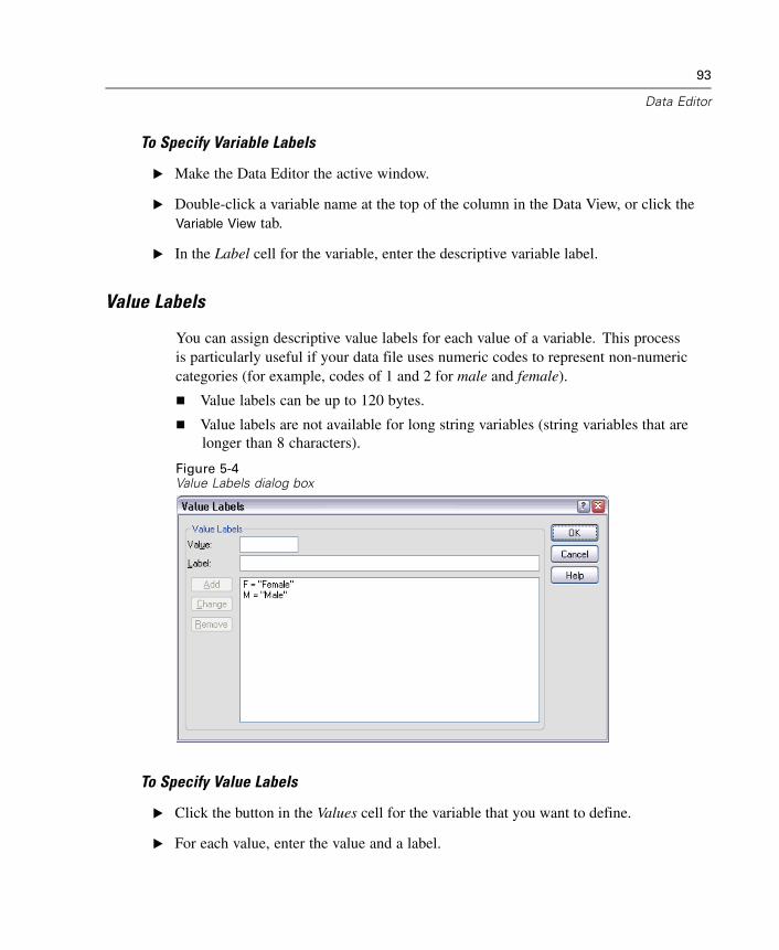
93

Data Editor

To Specify Variable Labels


E Double-click a variable name at the top of the column in the Data View, or click theVariable View tab.

E In the Label cell for the variable, enter the descriptive variable label.

Value Labels

You can assign descriptive value labels for each value of a variable. This processis particularly useful if your data file uses numeric codes to represent non-numericcategories (for example, codes of 1 and 2 for male and female).

Value labels can be up to 120 bytes.

Value labels are not available for long string variables (string variables that arelonger than 8 characters).

Figure 5-4Value Labels dialog box

To Specify Value Labels

E Click the button in the Values cell for the variable that you want to define.

E For each value, enter the value and a label.

94

Chapter 5

E Click Add to enter the value label.

E Click OK.

Inserting Line Breaks in Labels

Variable labels and value labels automatically wrap to multiple lines in pivot tablesand charts if the cell or area isn’t wide enough to display the entire label on one line,and you can edit results to insert manual line breaks if you want the label to wrap at adifferent point. You can also create variable labels and value labels that will alwayswrap at specified points and be displayed on multiple lines.

E For variable labels, select the Label cell for the variable in the Variable View in theData Editor.

E For value labels, select the Values cell for the variable in the Variable View in theData Editor, click the button in the cell, and in the Value Labels dialog box, select thelabel that you want to modify.

E At the place in the label where you want the label to wrap, type \n.

The \n is not displayed in pivot tables or charts; it is interpreted as a line break character.

Missing Values

Missing Values defines specified data values as user-missing. For example, you mightwant to distinguish between data that are missing because a respondent refused toanswer and data that are missing because the question didn’t apply to that respondent.Data values that are specified as user-missing are flagged for special treatment and areexcluded from most calculations.

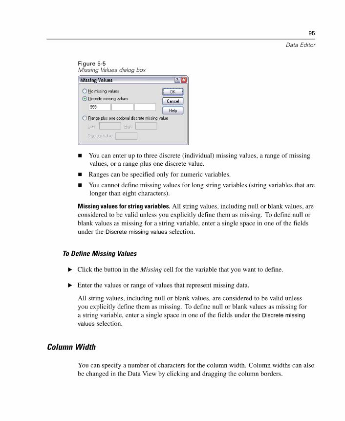
95

Data Editor

Figure 5-5Missing Values dialog box

You can enter up to three discrete (individual) missing values, a range of missingvalues, or a range plus one discrete value.

Ranges can be specified only for numeric variables.

You cannot define missing values for long string variables (string variables that arelonger than eight characters).

Missing values for string variables. All string values, including null or blank values, areconsidered to be valid unless you explicitly define them as missing. To define null orblank values as missing for a string variable, enter a single space in one of the fieldsunder the Discrete missing values selection.

To Define Missing Values

E Click the button in the Missing cell for the variable that you want to define.

E Enter the values or range of values that represent missing data.

All string values, including null or blank values, are considered to be valid unlessyou explicitly define them as missing. To define null or blank values as missing fora string variable, enter a single space in one of the fields under the Discrete missing

values selection.

Column Width

You can specify a number of characters for the column width. Column widths can alsobe changed in the Data View by clicking and dragging the column borders.

96

Chapter 5

Column formats affect only the display of values in the Data Editor. Changing thecolumn width does not change the defined width of a variable. If the defined and actualwidth of a value are wider than the column, asterisks (*) are displayed in the Data View.

Variable AlignmentAlignment controls the display of data values and/or value labels in the Data View.The default alignment is right for numeric variables and left for string variables. Thissetting affects only the display in the Data View.

Applying Variable Definition Attributes to Multiple Variables

After you have defined variable definition attributes for a variable, you can copy one ormore attributes and apply them to one or more variables.

Basic copy and paste operations are used to apply variable definition attributes. Youcan:

Copy a single attribute (for example, value labels) and paste it to the same attributecell(s) for one or more variables.

Copy all attributes from one variable and paste them to one or more other variables.

Create multiple new variables with all the attributes of a copied variable.

Applying Variable Definition Attributes to Other Variables

To apply individual attributes from a defined variable:

E In the Variable View, select the attribute cell that you want to apply to other variables.

E From the menus choose:Edit

Copy

E Select the attribute cell(s) to which you want to apply the attribute. (You can selectmultiple target variables.)


Paste

97

Data Editor

If you paste the attribute to blank rows, new variables are created with default attributesfor all attributes except the selected attribute.

To apply all attributes from a defined variable:

E In the Variable View, select the row number for the variable with the attributes that youwant to use. (The entire row is highlighted.)


Copy

E Select the row number(s) for the variable(s) to which you want to apply the attributes.(You can select multiple target variables.)


Paste

Generating Multiple New Variables with the Same Attributes

E In the Variable View, click the row number for the variable that has the attributes thatyou want to use for the new variable. (The entire row is highlighted.)


Copy

E Click the empty row number beneath the last defined variable in the data file.


Paste Variables...

E In the Paste Variables dialog box, enter the number of variables that you want to create.

E Enter a prefix and starting number for the new variables.

E Click OK.

The new variable names will consist of the specified prefix plus a sequential numberstarting with the specified number.

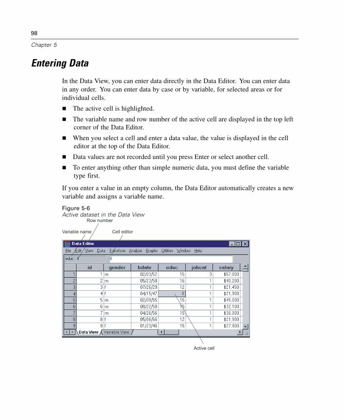
98

Chapter 5

Entering Data

In the Data View, you can enter data directly in the Data Editor. You can enter datain any order. You can enter data by case or by variable, for selected areas or forindividual cells.

The active cell is highlighted.

The variable name and row number of the active cell are displayed in the top leftcorner of the Data Editor.

When you select a cell and enter a data value, the value is displayed in the celleditor at the top of the Data Editor.

Data values are not recorded until you press Enter or select another cell.

To enter anything other than simple numeric data, you must define the variabletype first.

If you enter a value in an empty column, the Data Editor automatically creates a newvariable and assigns a variable name.

Figure 5-6Active dataset in the Data View

99

Data Editor

To Enter Numeric Data

E Select a cell in the Data View.

E Enter the data value. (The value is displayed in the cell editor at the top of the DataEditor.)

E To record the value, press Enter or select another cell.

To Enter Non-Numeric Data

E Double-click a variable name at the top of the column in the Data View or click theVariable View tab.

E Click the button in the Type cell for the variable.

E Select the data type in the Variable Type dialog box.

E Click OK.

E Double-click the row number or click the Data View tab.

E Enter the data in the column for the newly defined variable.

To Use Value Labels for Data Entry

E If value labels aren’t currently displayed in the Data View, from the menus choose:View

Value Labels

E Click the cell in which you want to enter the value.

E Choose a value label from the drop-down list.

The value is entered, and the value label is displayed in the cell.

Note: This process works only if you have defined value labels for the variable.

Data Value Restrictions in the Data Editor

The defined variable type and width determine the type of value that can be entered inthe cell in the Data View.

100

Chapter 5

If you type a character that is not allowed by the defined variable type, the DataEditor beeps and does not enter the character.

For string variables, characters beyond the defined width are not allowed.

For numeric variables, integer values that exceed the defined width can be entered,but the Data Editor displays either scientific notation or asterisks in the cell toindicate that the value is wider than the defined width. To display the value inthe cell, change the defined width of the variable. (Note: Changing the columnwidth does not affect the variable width.)

Editing Data

With the Data Editor, you can modify data values in the Data View in many ways.You can:

Change data values.

Cut, copy, and paste data values.

Add and delete cases.

Add and delete variables.

Change the order of variables.

Replacing or Modifying Data Values

To delete the old value and enter a new value:

E In the Data View, double-click the cell. (The cell value is displayed in the cell editor.)

E Edit the value directly in the cell or in the cell editor.

E Press Enter (or move to another cell) to record the new value.

Cutting, Copying, and Pasting Data Values

You can cut, copy, and paste individual cell values or groups of values in the DataEditor. You can:

Move or copy a single cell value to another cell.

Move or copy a single cell value to a group of cells.

101

Data Editor

Move or copy the values for a single case (row) to multiple cases.

Move or copy the values for a single variable (column) to multiple variables.

Move or copy a group of cell values to another group of cells.

Data Conversion for Pasted Values in the Data Editor

If the defined variable types of the source and target cells are not the same, the DataEditor attempts to convert the value. If no conversion is possible, the system-missingvalue is inserted in the target cell.

Converting Numeric or Date into String. Numeric (for example, numeric, dollar, dot,or comma) and date formats are converted to strings if they are pasted into a stringvariable cell. The string value is the numeric value as displayed in the cell. Forexample, for a dollar format variable, the displayed dollar sign becomes part of thestring value. Values that exceed the defined string variable width are truncated.

Converting String into Numeric or Date. String values that contain acceptable charactersfor the numeric or date format of the target cell are converted to the equivalent numericor date value. For example, a string value of 25/12/91 is converted to a valid dateif the format type of the target cell is one of the day-month-year formats, but thevalue is converted to system-missing if the format type of the target cell is one of themonth-day-year formats.

Converting Date into Numeric. Date and time values are converted to a number ofseconds if the target cell is one of the numeric formats (for example, numeric, dollar,dot, or comma). Because dates are stored internally as the number of seconds sinceOctober 14, 1582, converting dates to numeric values can yield some extremelylarge numbers. For example, the date 10/29/91 is converted to a numeric value of12,908,073,600.

Converting Numeric into Date or Time. Numeric values are converted to dates or times ifthe value represents a number of seconds that can produce a valid date or time. Fordates, numeric values that are less than 86,400 are converted to the system-missingvalue.

102

Chapter 5

Inserting New Cases

Entering data in a cell in a blank row automatically creates a new case. The Data Editorinserts the system-missing value for all other variables for that case. If there are anyblank rows between the new case and the existing cases, the blank rows become newcases with the system-missing value for all variables. You can also insert new casesbetween existing cases.

To Insert New Cases between Existing Cases

E In the Data View, select any cell in the case (row) below the position where you wantto insert the new case.


Insert Cases

A new row is inserted for the case, and all variables receive the system-missing value.

Inserting New Variables

Entering data in an empty column in the Data View or in an empty row in the VariableView automatically creates a new variable with a default variable name (the prefix varand a sequential number) and a default data format type (numeric). The Data Editorinserts the system-missing value for all cases for the new variable. If there are anyempty columns in the Data View or empty rows in the Variable View between the newvariable and the existing variables, these rows or columns also become new variableswith the system-missing value for all cases. You can also insert new variables betweenexisting variables.

To Insert New Variables between Existing Variables

E Select any cell in the variable to the right of (Data View) or below (Variable View) theposition where you want to insert the new variable.


Insert Variable

A new variable is inserted with the system-missing value for all cases.

103

Data Editor

To Move Variables

E To select the variable, click the variable name in the Data View or the row number forthe variable in the Variable View.

E Drag and drop the variable to the new location.

E If you want to place the variable between two existing variables: In the Data View,drop the variable on the variable column to the right of where you want to place thevariable, or in the Variable View, drop the variable on the variable row below whereyou want to place the variable.

To Change Data Type

You can change the data type for a variable at any time by using the Variable Typedialog box in the Variable View. The Data Editor will attempt to convert existingvalues to the new type. If no conversion is possible, the system-missing value isassigned. The conversion rules are the same as the rules for pasting data values to avariable with a different format type. If the change in data format may result in the lossof missing-value specifications or value labels, the Data Editor displays an alert boxand asks whether you want to proceed with the change or cancel it.

Go to Case

The Go to Case dialog box allows you to go to the specified case (row) numberin the Data Editor.

Figure 5-7Go to Case dialog box

To Find a Case in the Data Editor


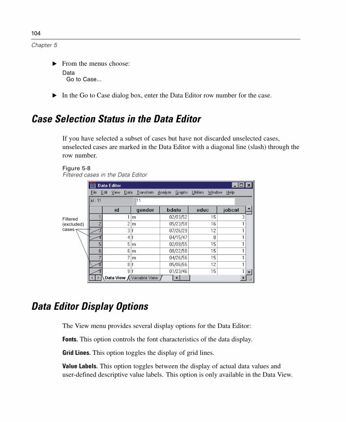
104

Chapter 5

E From the menus choose:Data

Go to Case...

E In the Go to Case dialog box, enter the Data Editor row number for the case.

Case Selection Status in the Data Editor

If you have selected a subset of cases but have not discarded unselected cases,unselected cases are marked in the Data Editor with a diagonal line (slash) through therow number.

Figure 5-8Filtered cases in the Data Editor

Filtered (excluded) cases

Data Editor Display Options

The View menu provides several display options for the Data Editor:

Fonts. This option controls the font characteristics of the data display.

Grid Lines. This option toggles the display of grid lines.

Value Labels. This option toggles between the display of actual data values anduser-defined descriptive value labels. This option is only available in the Data View.

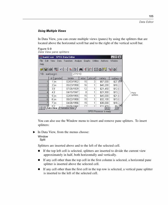
105

Data Editor

Using Multiple Views

In Data View, you can create multiple views (panes) by using the splitters that arelocated above the horizontal scroll bar and to the right of the vertical scroll bar.

Figure 5-9Data View pane splitters

Panesplitters

You can also use the Window menu to insert and remove pane splitters. To insertsplitters:

E In Data View, from the menus choose:Window

Split

Splitters are inserted above and to the left of the selected cell.

If the top left cell is selected, splitters are inserted to divide the current viewapproximately in half, both horizontally and vertically.

If any cell other than the top cell in the first column is selected, a horizontal panesplitter is inserted above the selected cell.

If any cell other than the first cell in the top row is selected, a vertical pane splitteris inserted to the left of the selected cell.

106

Chapter 5

Data Editor Printing

A data file is printed as it appears on the screen.

The information in the currently displayed view is printed. In the Data View, thedata are printed. In the Variable View, data definition information is printed.

Grid lines are printed if they are currently displayed in the selected view.

Value labels are printed in the Data View if they are currently displayed. Otherwise,the actual data values are printed.

Use the View menu in the Data Editor window to display or hide grid lines and togglebetween the display of data values and value labels.

To Print Data Editor Contents


E Click the tab for the view that you want to print.


Print...

Chapter

6Working with Multiple DataSources

Starting with SPSS 14.0, SPSS can have multiple data sources open at the same time,making it easier to:

Switch back and forth between data sources.

Compare the contents of different data sources.

Copy and paste data between data sources.

Create multiple subsets of cases and/or variables for analysis.

Merge multiple data sources from various data formats (for example, spreadsheet,database, text data) without saving each data source in SPSS format first.

107

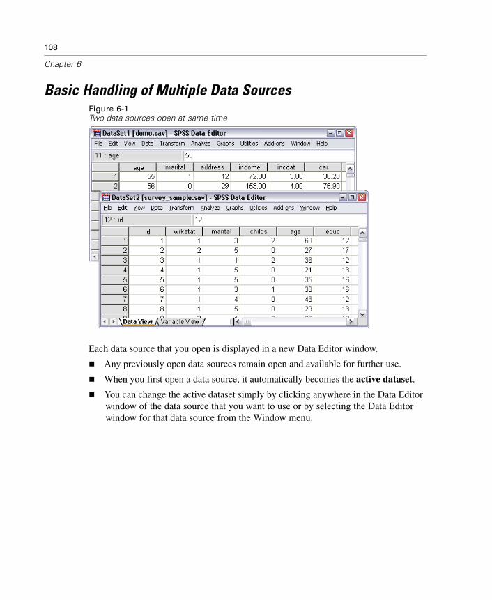
108

Chapter 6

Basic Handling of Multiple Data SourcesFigure 6-1Two data sources open at same time

Each data source that you open is displayed in a new Data Editor window.

Any previously open data sources remain open and available for further use.

When you first open a data source, it automatically becomes the active dataset.

You can change the active dataset simply by clicking anywhere in the Data Editorwindow of the data source that you want to use or by selecting the Data Editorwindow for that data source from the Window menu.

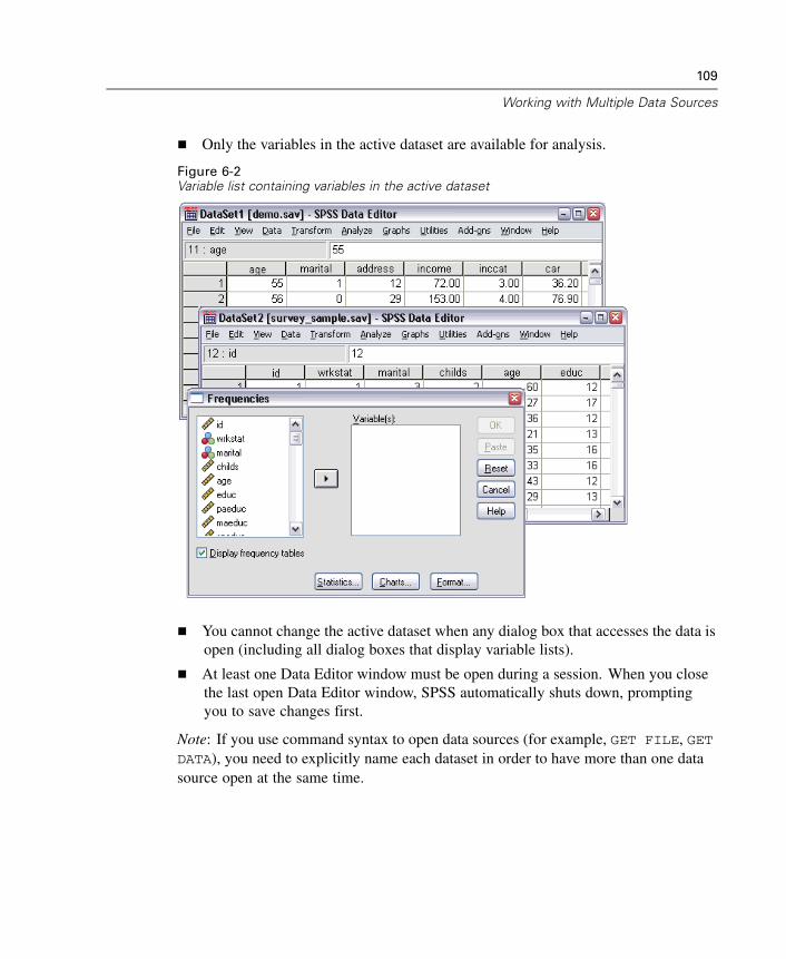
109

Working with Multiple Data Sources

Only the variables in the active dataset are available for analysis.

Figure 6-2Variable list containing variables in the active dataset

You cannot change the active dataset when any dialog box that accesses the data isopen (including all dialog boxes that display variable lists).

At least one Data Editor window must be open during a session. When you closethe last open Data Editor window, SPSS automatically shuts down, promptingyou to save changes first.

Note: If you use command syntax to open data sources (for example, GET FILE, GETDATA), you need to explicitly name each dataset in order to have more than one datasource open at the same time.

110

Chapter 6

Copying and Pasting Information between Datasets

You can copy both data and variable definition attributes from one dataset to anotherdataset in basically the same way that you copy and paste information within a singledata file.

Copying and pasting selected data cells in Data View pastes just the data values,with no variable definition attributes.

Copying and pasting an entire variable in Data View by selecting the variable nameat the top of the column pastes all of the data and all of the variable definitionattributes for that variable.

Copying and pasting variable definition attributes or entire variables in VariableView pastes the selected attributes (or the entire variable definition) but does notpaste any data values.

Renaming Datasets

When you open a data source through the menus and dialogs, each data source isautomatically assigned a dataset name of DataSetn, where n is a sequential integervalue, and when you open a data source via command syntax, no dataset name isassigned unless you explicitly specify one with DATASET NAME. To provide moredescriptive dataset names:

E From the menus in the Data Editor window for the dataset for which you want tochange the dataset name, choose:File

Rename Dataset

E Enter a new dataset name that conforms to SPSS variable naming rules. For moreinformation, see “Variable Names” in Chapter 5 on p. 88.

Chapter

7Data Preparation

Once you’ve opened a data file or entered data in the Data Editor, you can start creatingreports, charts, and analyses without any additional preliminary work. However, thereare some additional data preparation features that you may find useful, includingthe ability to:

Assign variable properties that describe the data and determine how certain valuesshould be treated.

Identify cases that may contain duplicate information and exclude those cases fromanalyses or delete them from the data file.

Create new variables with a few distinct categories that represent ranges of valuesfrom variables with a large number of possible values.

Variable Properties

Data entered in the Data Editor in Data View or read into SPSS from an external fileformat (such as an Excel spreadsheet or a text data file) lack certain variable propertiesthat you may find very useful, including:

Definition of descriptive value labels for numeric codes (for example, 0 = Maleand 1 = Female).

Identification of missing values codes (for example, 99 = Not applicable).

Assignment of measurement level (nominal, ordinal, or scale).

111

112

Chapter 7

All of these variable properties (and others) can be assigned in the Variable view of theData Editor. There are also several utilities that can assist you in this process:

Define Variable Properties can help you define descriptive value labels and missingvalues. This is particularly useful for categorical data with numeric codes usedfor category values.

Copy Data Properties provides the ability to use an existing SPSS-format datafile as a template for file and variable properties in the current data file. This isparticularly useful if you frequently use external-format data files that containsimilar content (such as monthly reports in Excel format).

Defining Variable Properties

Define Variable Properties is designed to assist you in the process of creatingdescriptive value labels for categorical (nominal, ordinal) variables. Define VariableProperties:

Scans the actual data values and lists all unique data values for each selectedvariable.

Identifies unlabeled values and provides an “auto-label” feature.

Provides the ability to copy defined value labels from another variable to theselected variable or from the selected variable to multiple additional variables.

Note: To use Define Variable Properties without first scanning cases, enter 0 for thenumber of cases to scan.

To Define Variable Properties


Define Variable Properties...

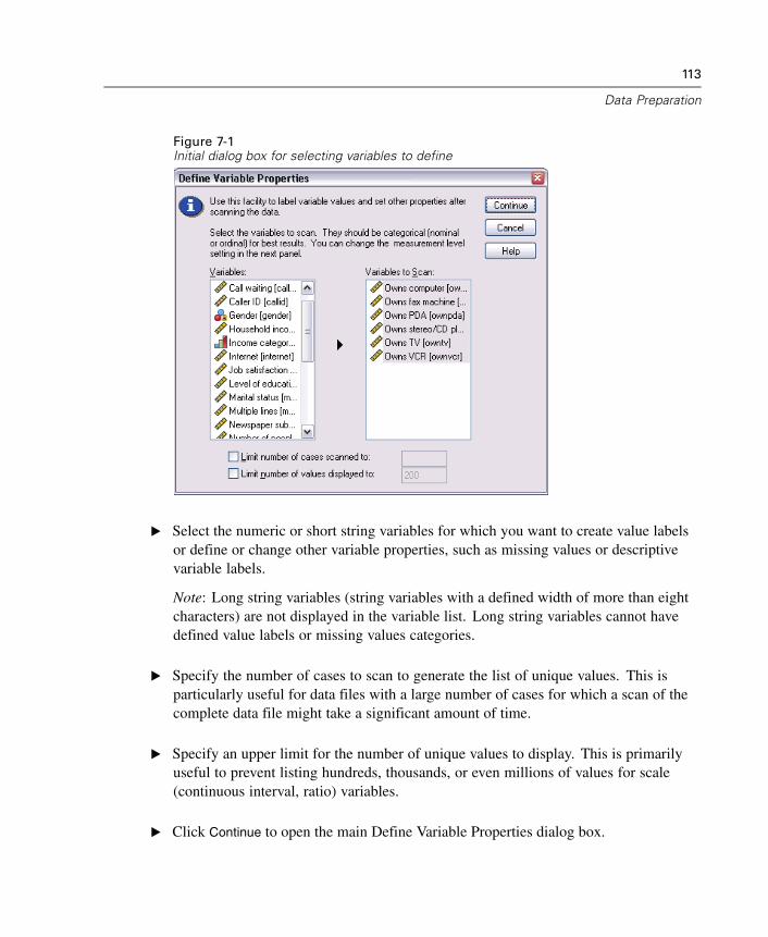
113

Data Preparation

Figure 7-1Initial dialog box for selecting variables to define

E Select the numeric or short string variables for which you want to create value labelsor define or change other variable properties, such as missing values or descriptivevariable labels.

Note: Long string variables (string variables with a defined width of more than eightcharacters) are not displayed in the variable list. Long string variables cannot havedefined value labels or missing values categories.

E Specify the number of cases to scan to generate the list of unique values. This isparticularly useful for data files with a large number of cases for which a scan of thecomplete data file might take a significant amount of time.

E Specify an upper limit for the number of unique values to display. This is primarilyuseful to prevent listing hundreds, thousands, or even millions of values for scale(continuous interval, ratio) variables.

E Click Continue to open the main Define Variable Properties dialog box.

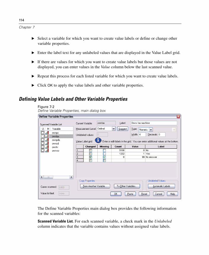
114

Chapter 7

E Select a variable for which you want to create value labels or define or change othervariable properties.

E Enter the label text for any unlabeled values that are displayed in the Value Label grid.

E If there are values for which you want to create value labels but those values are notdisplayed, you can enter values in the Value column below the last scanned value.

E Repeat this process for each listed variable for which you want to create value labels.

E Click OK to apply the value labels and other variable properties.

Defining Value Labels and Other Variable PropertiesFigure 7-2Define Variable Properties, main dialog box

The Define Variable Properties main dialog box provides the following informationfor the scanned variables:

Scanned Variable List. For each scanned variable, a check mark in the Unlabeledcolumn indicates that the variable contains values without assigned value labels.

115

Data Preparation

To sort the variable list to display all variables with unlabeled values at the top ofthe list:

E Click the Unlabeled column heading under Scanned Variable List.

You can also sort by variable name or measurement level by clicking the correspondingcolumn heading under Scanned Variable List.

Value Label Grid

Label. Displays any value labels that have already been defined. You can add orchange labels in this column.

Value. Unique values for each selected variable. This list of unique values is basedon the number of scanned cases. For example, if you scanned only the first 100cases in the data file, then the list reflects only the unique values present in thosecases. If the data file has already been sorted by the variable for which you want toassign value labels, the list may display far fewer unique values than are actuallypresent in the data.

Count. The number of times each value occurs in the scanned cases.

Missing. Values defined as representing missing data. You can change the missingvalues designation of the category by clicking the check box. A check indicatesthat the category is defined as a user-missing category. If a variable already has arange of values defined as user-missing (for example, 90-99), you cannot add ordelete missing values categories for that variable with Define Variable Properties.You can use the Variable view of the Data Editor to modify the missing valuescategories for variables with missing values ranges. For more information, see“Missing Values” in Chapter 5 on p. 94.

Changed. Indicates that you have added or changed a value label.

Note: If you specified 0 for the number of cases to scan in the initial dialog box, theValue Label grid will initially be blank, except for any preexisting value labels and/ordefined missing values categories for the selected variable. In addition, the Suggest

button for the measurement level will be disabled.

Measurement Level. Value labels are primarily useful for categorical (nominal andordinal) variables, and some procedures treat categorical and scale variables differently;so it is sometimes important to assign the correct measurement level. However, bydefault, all new numeric variables are assigned the scale measurement level. Thus,many variables that are in fact categorical may initially be displayed as scale.

116

Chapter 7

If you are unsure of what measurement level to assign to a variable, click Suggest.

Copy Properties. You can copy value labels and other variable properties from anothervariable to the currently selected variable or from the currently selected variable to oneor more other variables.

Unlabeled Values. To create labels for unlabeled values automatically, click Automatic

Labels.

Variable Label and Display Format

You can change the descriptive variable label and the display format.

You cannot change the variable’s fundamental type (string or numeric).

For string variables, you can change only the variable label, not the display format.

For numeric variables, you can change the numeric type (such as numeric, date,dollar, or custom currency), width (maximum number of digits, including anydecimal and/or grouping indicators), and number of decimal positions.

For numeric date format, you can select a specific date format (such asdd-mm-yyyy, mm/dd/yy, yyyyddd, etc.)

For numeric custom format, you can select one of five custom currency formats(CCA through CCE). For more information, see “Currency Options” in Chapter44 on p. 611.

An asterisk is displayed in the Value column if the specified width is less than thewidth of the scanned values or the displayed values for preexisting defined valuelabels or missing values categories.

A period (.) is displayed if the scanned values or the displayed values forpreexisting defined value labels or missing values categories are invalid for theselected display format type. For example, an internal numeric value of less than86,400 is invalid for a date format variable.

Assigning the Measurement Level

When you click Suggest for the measurement level in the Define Variable Propertiesmain dialog box, the current variable is evaluated based on the scanned cases anddefined value labels, and a measurement level is suggested in the Suggest MeasurementLevel dialog box that opens. The Explanation area provides a brief description of thecriteria used to provide the suggested measurement level.

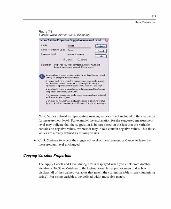
117

Data Preparation

Figure 7-3Suggest Measurement Level dialog box

Note: Values defined as representing missing values are not included in the evaluationfor measurement level. For example, the explanation for the suggested measurementlevel may indicate that the suggestion is in part based on the fact that the variablecontains no negative values, whereas it may in fact contain negative values—but thosevalues are already defined as missing values.

E Click Continue to accept the suggested level of measurement or Cancel to leave themeasurement level unchanged.

Copying Variable Properties

The Apply Labels and Level dialog box is displayed when you click From Another

Variable or To Other Variables in the Define Variable Properties main dialog box. Itdisplays all of the scanned variables that match the current variable’s type (numeric orstring). For string variables, the defined width must also match.

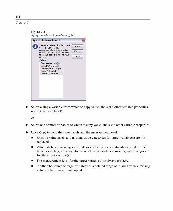
118

Chapter 7

Figure 7-4Apply Labels and Level dialog box

E Select a single variable from which to copy value labels and other variable properties(except variable label).

or

E Select one or more variables to which to copy value labels and other variable properties.

E Click Copy to copy the value labels and the measurement level.

Existing value labels and missing value categories for target variable(s) are notreplaced.

Value labels and missing value categories for values not already defined for thetarget variable(s) are added to the set of value labels and missing value categoriesfor the target variable(s).

The measurement level for the target variable(s) is always replaced.

If either the source or target variable has a defined range of missing values, missingvalues definitions are not copied.

119

Data Preparation

Multiple Response Sets

Custom Tables and the Chart Builder support a special kind of “variable” called amultiple response set. Multiple response sets aren’t really “variables” in the normalsense. You can’t see them in the Data Editor, and other procedures don’t recognizethem. Multiple response sets use multiple variables to record responses to questionswhere the respondent can give more than one answer. Multiple response sets aretreated like categorical variables, and most of the things you can do with categoricalvariables, you can also do with multiple response sets.

Multiple response sets are constructed from multiple variables in the data file.A multiple response set is a special construct within an SPSS-format data file. Youcan define and save multiple sets in an SPSS-format data file, but you cannot importor export multiple response sets from/to other file formats. (You can copy multipleresponse sets from other SPSS data files using Copy Data Properties, which is accessedfrom the Data menu in the Data Editor window. For more information, see “CopyingData Properties” on p. 122.)

Defining Multiple Response Sets

To define multiple response sets:

E From the menus, choose:Data

Define Multiple Response Sets...

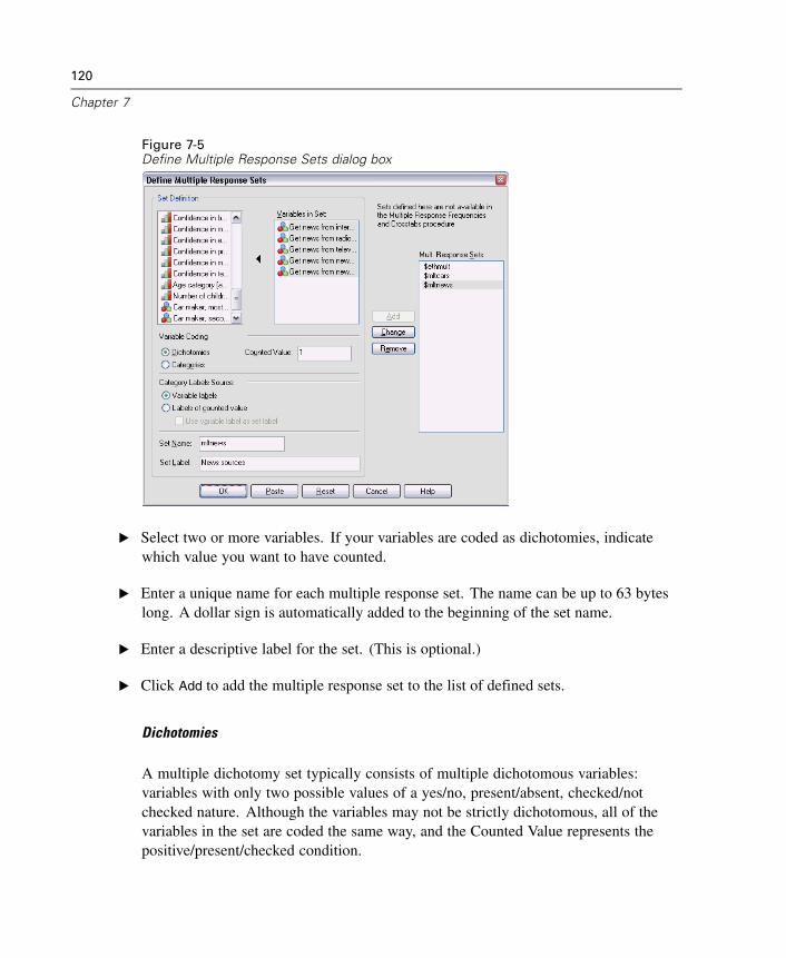
120

Chapter 7

Figure 7-5Define Multiple Response Sets dialog box

E Select two or more variables. If your variables are coded as dichotomies, indicatewhich value you want to have counted.

E Enter a unique name for each multiple response set. The name can be up to 63 byteslong. A dollar sign is automatically added to the beginning of the set name.

E Enter a descriptive label for the set. (This is optional.)

E Click Add to add the multiple response set to the list of defined sets.

Dichotomies

A multiple dichotomy set typically consists of multiple dichotomous variables:variables with only two possible values of a yes/no, present/absent, checked/notchecked nature. Although the variables may not be strictly dichotomous, all of thevariables in the set are coded the same way, and the Counted Value represents thepositive/present/checked condition.

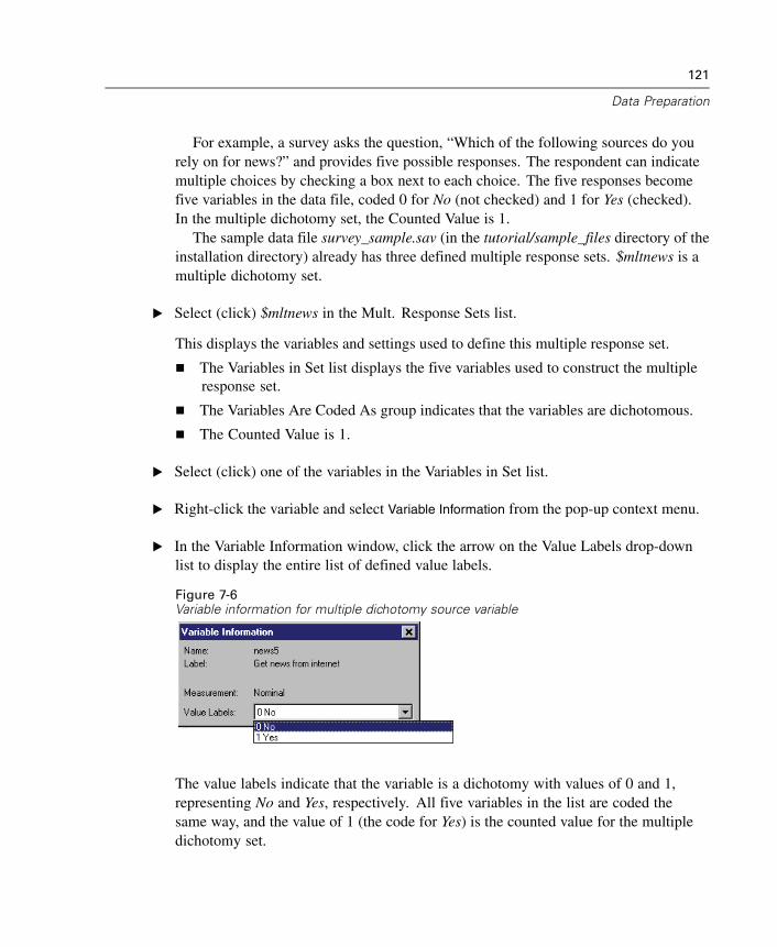
121

Data Preparation

For example, a survey asks the question, “Which of the following sources do yourely on for news?” and provides five possible responses. The respondent can indicatemultiple choices by checking a box next to each choice. The five responses becomefive variables in the data file, coded 0 for No (not checked) and 1 for Yes (checked).In the multiple dichotomy set, the Counted Value is 1.

The sample data file survey_sample.sav (in the tutorial/sample_files directory of theinstallation directory) already has three defined multiple response sets. $mltnews is amultiple dichotomy set.

E Select (click) $mltnews in the Mult. Response Sets list.

This displays the variables and settings used to define this multiple response set.

The Variables in Set list displays the five variables used to construct the multipleresponse set.

The Variables Are Coded As group indicates that the variables are dichotomous.

The Counted Value is 1.

E Select (click) one of the variables in the Variables in Set list.

E Right-click the variable and select Variable Information from the pop-up context menu.

E In the Variable Information window, click the arrow on the Value Labels drop-downlist to display the entire list of defined value labels.

Figure 7-6Variable information for multiple dichotomy source variable

The value labels indicate that the variable is a dichotomy with values of 0 and 1,representing No and Yes, respectively. All five variables in the list are coded thesame way, and the value of 1 (the code for Yes) is the counted value for the multipledichotomy set.

122

Chapter 7

Categories

A multiple category set consists of multiple variables, all coded the same way, oftenwith many possible response categories. For example, a survey item states, “Name upto three nationalities that best describe your ethnic heritage.” There may be hundreds ofpossible responses, but for coding purposes the list is limited to the 40 most commonnationalities, with everything else relegated to an “other” category. In the data file, thethree choices become three variables, each with 41 categories (40 coded nationalitiesand one “other” category).

In the sample data file, $ethmult and $mltcars are multiple category sets.

Category Label Source

For multiple dichotomies, you can control how sets are labeled.

Variable labels. Uses the defined variable labels (or variable names for variableswithout defined variable labels) as the set category labels. For example, if all ofthe variables in the set have the same value label (or no defined value labels) forthe counted value (for example, Yes), then you should use the variable labels asthe set category labels.

Labels of counted values. Uses the defined value labels of the counted values asset category labels. Select this option only if all variables have a defined valuelabel for the counted value and the value label for the counted value is differentfor each variable.

Use variable label as set label. If you select Label of counted values, you can alsouse the variable label for the first variable in the set with a defined variable label asthe set label. If none of the variables in the set have defined variable labels, thename of the first variable in the set is used as the set label.

Copying Data PropertiesThe Copy Data Properties Wizard provides the ability to use an external SPSS data fileas a template for defining file and variable properties in the active dataset. You canalso use variables in the active dataset as templates for other variables in the activedataset. You can:

Copy selected file properties from an external data file or open dataset to the activedataset. File properties include documents, file labels, multiple response sets,variable sets, and weighting.

123

Data Preparation

Copy selected variable properties from an external data file or open dataset tomatching variables in the active dataset. Variable properties include value labels,missing values, level of measurement, variable labels, print and write formats,alignment, and column width (in the Data Editor).

Copy selected variable properties from one variable in either an external data file,open dataset, or the active dataset to many variables in the active dataset.

Create new variables in the active dataset based on selected variables in an externaldata file or open dataset.

When copying data properties, the following general rules apply:

If you use an external data file as the source data file, it must be an SPSS-formatdata file.

If you use the active dataset as the source data file, it must contain at least onevariable. You cannot use a completely blank active dataset as the source data file.

Undefined (empty) properties in the source dataset do not overwrite definedproperties in the active dataset.

Variable properties are copied from the source variable only to target variables ofa matching type—string (alphanumeric) or numeric (including numeric, date,and currency).

Note: Copy Data Properties replaces Apply Data Dictionary, formerly available onthe File menu.

To Copy Data Properties

E From the menus in the Data Editor window choose:Data

Copy Data Properties...

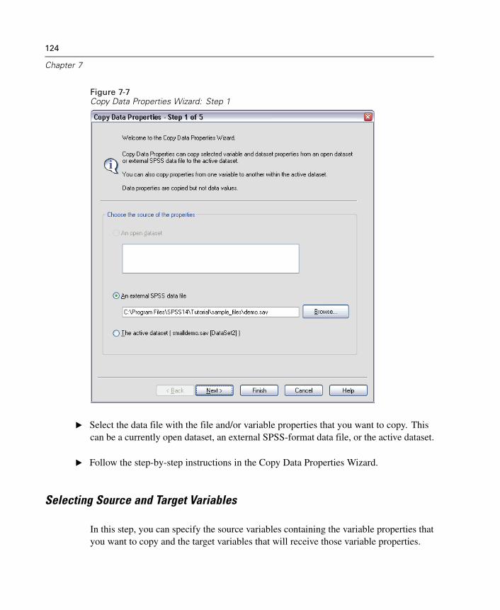
124

Chapter 7

Figure 7-7Copy Data Properties Wizard: Step 1

E Select the data file with the file and/or variable properties that you want to copy. Thiscan be a currently open dataset, an external SPSS-format data file, or the active dataset.

E Follow the step-by-step instructions in the Copy Data Properties Wizard.

Selecting Source and Target Variables

In this step, you can specify the source variables containing the variable properties thatyou want to copy and the target variables that will receive those variable properties.

125

Data Preparation


Apply properties from selected source dataset variables to matching active datasetvariables. Variable properties are copied from one or more selected source variablesto matching variables in the active dataset. Variables “match” if both the variablename and type (string or numeric) are the same. For string variables, the definedlength must also be the same. By default, only matching variables are displayed in thetwo variable lists.

Create matching variables in the active dataset if they do not already exist. Thisupdates the source list to display all variables in the source data file. If you selectsource variables that do not exist in the active dataset (based on variable name),

126

Chapter 7

new variables will be created in the active dataset with the variable names andproperties from the source data file.

If the active dataset contains no variables (a blank, new dataset), all variables in thesource data file are displayed and new variables based on the selected source variablesare automatically created in the active dataset.

Apply properties from a single source variable to selected active dataset variables of thesame type. Variable properties from a single selected variable in the source list can beapplied to one or more selected variables in the active dataset list. Only variables of thesame type (numeric or string) as the selected variable in the source list are displayedin the active dataset list. For string variables, only strings of the same defined lengthas the source variable are displayed. This option is not available if the active datasetcontains no variables.

Note: You cannot create new variables in the active dataset with this option.

Apply dataset properties only—no variable selection. Only file properties (for example,documents, file label, weight) will be applied to the active dataset. No variableproperties will be applied. This option is not available if the active dataset is alsothe source data file.

Choosing Variable Properties to Copy

You can copy selected variable properties from the source variables to the targetvariables. Undefined (empty) properties in the source variables do not overwritedefined properties in the target variables.

127

Data Preparation


Value Labels. Value labels are descriptive labels associated with data values. Valuelabels are often used when numeric data values are used to represent non-numericcategories (for example, codes of 1 and 2 for Male and Female). You can replace ormerge value labels in the target variables.

Replace deletes any defined value labels for the target variable and replaces themwith the defined value labels from the source variable.

Merge merges the defined value labels from the source variable with any existingdefined value label for the target variable. If the same value has a defined valuelabel in both the source and target variables, the value label in the target variableis unchanged.

128

Chapter 7

Custom Attributes. Custom variable attributes, typically created by the VARIABLEATTRIBUTE command in command syntax.

Replace deletes any custom attributes for the target variable and replaces them withthe defined attributes from the source variable.

Merge merges the defined attributes from the source variable with any existingdefined attributes for the target variable.

Missing Values. Missing values are values identified as representing missing data (forexample, 98 for Do not know and 99 for Not applicable). Typically, these values alsohave defined value labels that describe what the missing value codes stand for. Anyexisting defined missing values for the target variable are deleted and replaced with thedefined missing values from the source variable.

Variable Label. Descriptive variable labels can contain spaces and reserved charactersnot allowed in variable names. If you’re copying variable properties from a singlesource variable to multiple target variables, you might want to think twice beforeselecting this option.

Measurement Level. The measurement level can be nominal, ordinal, or scale. Forthose procedures that distinguish between different measurement levels, nominal andordinal are both considered categorical.

Formats. For numeric variables, this controls numeric type (such as numeric, date, orcurrency), width (total number of displayed characters, including leading and trailingcharacters and decimal indicator), and number of decimal places displayed. Thisoption is ignored for string variables.

Alignment. This affects only alignment (left, right, center) in the Data view in theData Editor.

Data Editor Column Width. This affects only column width in the Data view in the DataEditor.

Copying Dataset (File) Properties

You can apply selected, global dataset properties from the source data file to the activedataset. (This is not available if the active dataset is the source data file.)

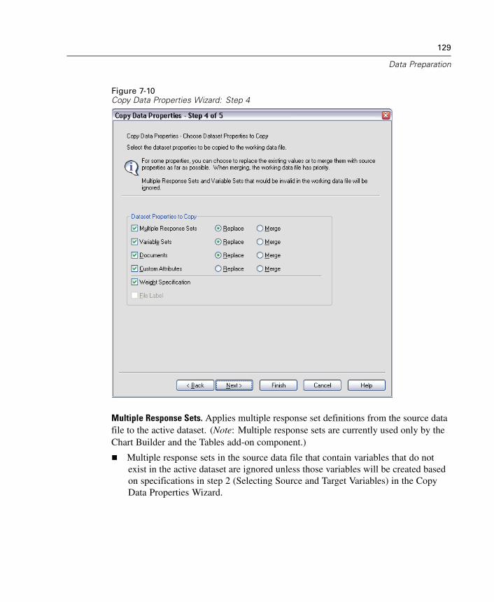
129

Data Preparation


Multiple Response Sets. Applies multiple response set definitions from the source datafile to the active dataset. (Note: Multiple response sets are currently used only by theChart Builder and the Tables add-on component.)

Multiple response sets in the source data file that contain variables that do notexist in the active dataset are ignored unless those variables will be created basedon specifications in step 2 (Selecting Source and Target Variables) in the CopyData Properties Wizard.

130

Chapter 7

Replace deletes all multiple response sets in the active dataset and replaces themwith the multiple response sets from the source data file.

Merge adds multiple response sets from the source data file to the collection ofmultiple response sets in the active dataset. If a set with the same name exists inboth files, the existing set in the active dataset is unchanged.

Variable Sets. Variable sets are used to control the list of variables that are displayed indialog boxes. Variable sets are defined by selecting Define Sets from the Utilities menu.

Sets in the source data file that contain variables that do not exist in the activedataset are ignored unless those variables will be created based on specifications instep 2 (Selecting Source and Target Variables) in the Copy Data Properties Wizard.

Replace deletes any existing variable sets in the active dataset, replacing them withvariable sets from the source data file.

Merge adds variable sets from the source data file to the collection of variable setsin the active dataset. If a set with the same name exists in both files, the existingset in the active dataset is unchanged.

Documents. Notes appended to the data file via the DOCUMENT command.

Replace deletes any existing documents in the active dataset, replacing them withthe documents from the source data file.

Merge combines documents from the source and active dataset. Unique documentsin the source file that do not exist in the active dataset are added to the activedataset. All documents are then sorted by date.

Custom Attributes. Custom data file attributes, typically created with the DATAFILEATTRIBUTE command in command syntax.

Replace deletes any existing custom data file attributes in the active dataset,replacing them with the data file attributes from the source data file.

Merge combines data file attributes from the source and active dataset. Uniqueattribute names in the source file that do not exist in the active dataset are added tothe active dataset. It the same attribute name exists in both data files, the namedattribute in the active dataset is unchanged.

Weight Specification. Weights cases by the current weight variable in the source datafile if there is a matching variable in the active dataset. This overrides any weightingcurrently in effect in the active dataset.

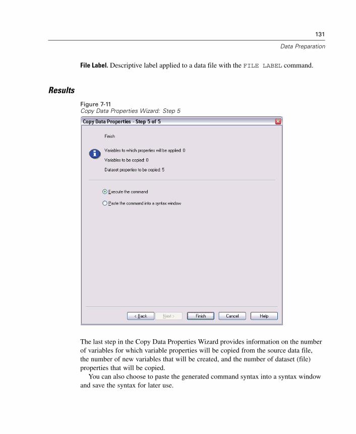
131

Data Preparation

File Label. Descriptive label applied to a data file with the FILE LABEL command.

ResultsFigure 7-11Copy Data Properties Wizard: Step 5

The last step in the Copy Data Properties Wizard provides information on the numberof variables for which variable properties will be copied from the source data file,the number of new variables that will be created, and the number of dataset (file)properties that will be copied.

You can also choose to paste the generated command syntax into a syntax windowand save the syntax for later use.

132

Chapter 7

Identifying Duplicate Cases

“Duplicate” cases may occur in your data for many reasons, including:

Data entry errors in which the same case is accidentally entered more than once.

Multiple cases share a common primary ID value but have different secondary IDvalues, such as family members who all live in the same house.

Multiple cases represent the same case but with different values for variables otherthan those that identify the case, such as multiple purchases made by the sameperson or company for different products or at different times.

Identify Duplicate Cases allows you to define duplicate almost any way that youwant and provides some control over the automatic determination of primary versusduplicate cases.

To Identify and Flag Duplicate Cases


Identify Duplicate Cases...

E Select one or more variables that identify matching cases.

E Select one or more of the options in the Variables to Create group.


E Select one or more variables to sort cases within groups defined by the selectedmatching cases variables. The sort order defined by these variables determines the“first” and “last” case in each group. Otherwise, the original file order is used.

E Automatically filter duplicate cases so that they won’t be included in reports, charts, orcalculation of statistics.

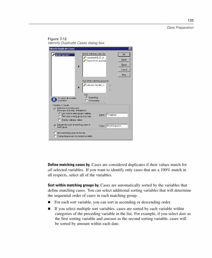
133

Data Preparation

Figure 7-12Identify Duplicate Cases dialog box

Define matching cases by. Cases are considered duplicates if their values match forall selected variables. If you want to identify only cases that are a 100% match inall respects, select all of the variables.

Sort within matching groups by. Cases are automatically sorted by the variables thatdefine matching cases. You can select additional sorting variables that will determinethe sequential order of cases in each matching group.

For each sort variable, you can sort in ascending or descending order.

If you select multiple sort variables, cases are sorted by each variable withincategories of the preceding variable in the list. For example, if you select date asthe first sorting variable and amount as the second sorting variable, cases willbe sorted by amount within each date.

134

Chapter 7

Use the up and down arrow buttons to the right of the list to change the sort orderof the variables.

The sort order determines the “first” and “last” case within each matching group,which determines the value of the optional primary indicator variable. Forexample, if you want to filter out all but the most recent case in each matchinggroup, you could sort cases within the group in ascending order of a date variable,which would make the most recent date the last date in the group.

Indicator of primary cases. Creates a variable with a value of 1 for all unique cases andthe case identified as the primary case in each group of matching cases and a value of 0for the nonprimary duplicates in each group.

The primary case can be either the last or first case in each matching group, asdetermined by the sort order within the matching group. If you don’t specifyany sort variables, the original file order determines the order of cases withineach group.

You can use the indicator variable as a filter variable to exclude nonprimaryduplicates from reports and analyses without deleting those cases from the data file.

Sequential count of matching cases in each group. Creates a variable with a sequentialvalue from 1 to n for cases in each matching group. The sequence is based on thecurrent order of cases in each group, which is either the original file order or the orderdetermined by any specified sort variables.

Move matching cases to the top. Sorts the data file so that all groups of matching casesare at the top of the data file, making it easy to visually inspect the matching casesin the Data Editor.

Display frequencies for created variables. Frequency tables containing counts for eachvalue of the created variables. For example, for the primary indicator variable, thetable would show the number of cases with a value 0 for that variable, which indicatesthe number of duplicates, and the number of cases with a value of 1 for that variable,which indicates the number of unique and primary cases.

Missing Values. For numeric variables, the system-missing value is treated like anyother value—cases with the system-missing value for an identifier variable are treatedas having matching values for that variable. For string variables, cases with no valuefor an identifier variable are treated as having matching values for that variable.

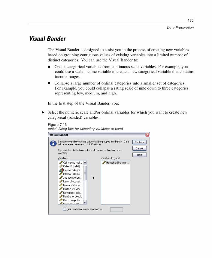
135

Data Preparation

Visual Bander

The Visual Bander is designed to assist you in the process of creating new variablesbased on grouping contiguous values of existing variables into a limited number ofdistinct categories. You can use the Visual Bander to:

Create categorical variables from continuous scale variables. For example, youcould use a scale income variable to create a new categorical variable that containsincome ranges.

Collapse a large number of ordinal categories into a smaller set of categories.For example, you could collapse a rating scale of nine down to three categoriesrepresenting low, medium, and high.

In the first step of the Visual Bander, you:

E Select the numeric scale and/or ordinal variables for which you want to create newcategorical (banded) variables.

Figure 7-13Initial dialog box for selecting variables to band

136

Chapter 7

Optionally, you can limit the number of cases to scan. For data files with a largenumber of cases, limiting the number of cases scanned can save time, but you shouldavoid this if possible because it will affect the distribution of values used in subsequentcalculations in the Visual Bander.

Note: String variables and nominal numeric variables are not displayed in the sourcevariable list. The Visual Bander requires numeric variables, measured on either ascale or ordinal level, since it assumes that the data values represent some logicalorder that can be used to group values in a meaningful fashion. You can change thedefined measurement level of a variable in Variable View in the Data Editor. For moreinformation, see “Variable Measurement Level” in Chapter 5 on p. 89.

To Band Variables

E From the menus in the Data Editor window choose:Transform

Visual Bander...

E Select the numeric scale and/or ordinal variables for which you want to create newcategorical (banded) variables.

E Select a variable in the Scanned Variable List.

E Enter a name for the new banded variable. Variable names must be unique and mustfollow SPSS variable naming rules. For more information, see “Variable Names”in Chapter 5 on p. 88.

E Define the banding criteria for the new variable. For more information, see “BandingVariables” on p. 137.

E Click OK.

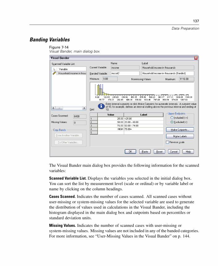
137

Data Preparation

Banding VariablesFigure 7-14Visual Bander, main dialog box

The Visual Bander main dialog box provides the following information for the scannedvariables:

Scanned Variable List. Displays the variables you selected in the initial dialog box.You can sort the list by measurement level (scale or ordinal) or by variable label orname by clicking on the column headings.

Cases Scanned. Indicates the number of cases scanned. All scanned cases withoutuser-missing or system-missing values for the selected variable are used to generatethe distribution of values used in calculations in the Visual Bander, including thehistogram displayed in the main dialog box and cutpoints based on percentiles orstandard deviation units.

Missing Values. Indicates the number of scanned cases with user-missing orsystem-missing values. Missing values are not included in any of the banded categories.For more information, see “User-Missing Values in the Visual Bander” on p. 144.

138

Chapter 7

Current Variable. The name and variable label (if any) for the currently selected variablethat will be used as the basis for the new, banded variable.

Banded Variable. Name and optional variable label for the new, banded variable.

Name. You must enter a name for the new variable. Variable names must be uniqueand must follow SPSS variable naming rules. For more information, see “VariableNames” in Chapter 5 on p. 88.

Label. You can enter a descriptive variable label up to 255 characters long. Thedefault variable label is the variable label (if any) or variable name of the sourcevariable with (Banded) appended to the end of the label.

Minimum and Maximum. Minimum and maximum values for the currently selectedvariable, based on the scanned cases and not including values defined as user-missing.

Nonmissing Values. The histogram displays the distribution of nonmissing values forthe currently selected variable, based on the scanned cases.

After you define bands for the new variable, vertical lines on the histogram aredisplayed to indicate the cutpoints that define bands.

You can click and drag the cutpoint lines to different locations on the histogram,changing the band ranges.

You can remove bands by dragging cutpoint lines off the histogram.

Note: The histogram (displaying nonmissing values), the minimum, and the maximumare based on the scanned values. If you do not include all cases in the scan, the truedistribution may not be accurately reflected, particularly if the data file has been sortedby the selected variable. If you scan zero cases, no information about the distributionof values is available.

Grid. Displays the values that define the upper endpoints of each band and optionalvalue labels for each band.

Value. The values that define the upper endpoints of each band. You can entervalues or use Make Cutpoints to automatically create bands based on selectedcriteria. By default, a cutpoint with a value of HIGH is automatically included.This band will contain any nonmissing values above the other cutpoints. The banddefined by the lowest cutpoint will include all nonmissing values lower than or

139

Data Preparation

equal to that value (or simply lower than that value, depending on how you defineupper endpoints).

Label. Optional, descriptive labels for the values of the new, banded variable. Sincethe values of the new variable will simply be sequential integers from 1 to n, labelsthat describe what the values represent can be very useful. You can enter labels oruse Make Labels to automatically create value labels.

To Delete a Band from the Grid

E Right-click on the either the Value or Label cell for the band.

E From the pop-up context menu, select Delete Row.

Note: If you delete the HIGH band, any cases with values higher than the last specifiedcutpoint value will be assigned the system-missing value for the new variable.

To Delete All Labels or Delete All Defined Bands

E Right-click anywhere in the grid.

E From the pop-up context menu select either Delete All Labels or Delete All Cutpoints.

Upper Endpoints. Controls treatment of upper endpoint values entered in the Valuecolumn of the grid.

Included (<=). Cases with the value specified in the Value cell are included in thebanded category. For example, if you specify values of 25, 50, and 75, cases witha value of exactly 25 will go in the first band, since this will include all caseswith values less than or equal to 25.

Excluded (<). Cases with the value specified in the Value cell are not included inthe banded category. Instead, they are included in the next band. For example, ifyou specify values of 25, 50, and 75, cases with a value of exactly 25 will go inthe second band rather than the first, since the first band will contain only caseswith values less than 25.

Make Cutpoints. Generates banded categories automatically for equal width intervals,intervals with the same number of cases, or intervals based on standard deviations. Thisis not available if you scanned zero cases. For more information, see “AutomaticallyGenerating Banded Categories” on p. 140.

140

Chapter 7

Make Labels. Generates descriptive labels for the sequential integer values of the new,banded variable, based on the values in the grid and the specified treatment of upperendpoints (included or excluded).

Reverse scale. By default, values of the new, banded variable are ascending sequentialintegers from 1 to n. Reversing the scale makes the values descending sequentialintegers from n to 1.

Copy Bands. You can copy the banding specifications from another variable to thecurrently selected variable or from the selected variable to multiple other variables. Formore information, see “Copying Banded Categories” on p. 143.

Automatically Generating Banded Categories

The Make Cutpoints dialog box allows you to auto-generate banded categories basedon selected criteria.

To Use the Make Cutpoints Dialog Box

E Select (click) a variable in the Scanned Variable List.

E Click Make Cutpoints.

E Select the criteria for generating cutpoints that will define the banded categories.

E Click Apply.

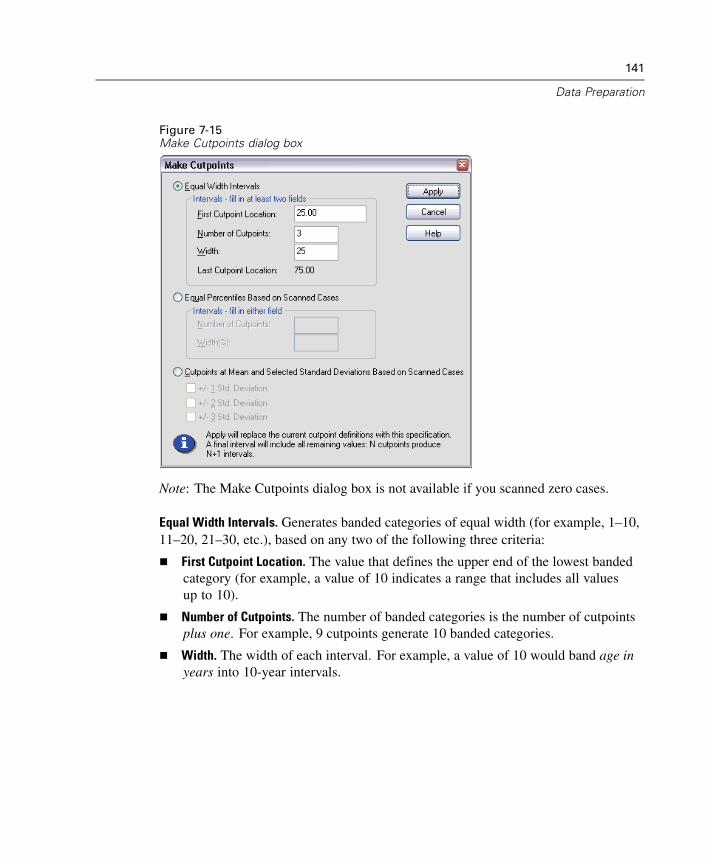
141

Data Preparation

Figure 7-15Make Cutpoints dialog box

Note: The Make Cutpoints dialog box is not available if you scanned zero cases.

Equal Width Intervals. Generates banded categories of equal width (for example, 1–10,11–20, 21–30, etc.), based on any two of the following three criteria:

First Cutpoint Location. The value that defines the upper end of the lowest bandedcategory (for example, a value of 10 indicates a range that includes all valuesup to 10).

Number of Cutpoints. The number of banded categories is the number of cutpointsplus one. For example, 9 cutpoints generate 10 banded categories.

Width. The width of each interval. For example, a value of 10 would band age inyears into 10-year intervals.

142

Chapter 7

Equal Percentiles Based on Scanned Cases. Generates banded categories with an equalnumber of cases in each band (using the aempirical algorithm for percentiles), basedon either of the following criteria:

Number of Cutpoints. The number of banded categories is the number of cutpointsplus one. For example, three cutpoints generate four percentile bands (quartiles),each containing 25% of the cases.

Width (%). Width of each interval, expressed as a percentage of the total number ofcases. For example, a value of 33.3 would produce three banded categories (twocutpoints), each containing 33.3% of the cases.

If the source variable contains a relatively small number of distinct values or a largenumber of cases with the same value, you may get fewer bands than requested. If thereare multiple identical values at a cutpoint, they will all go into the same interval; sothe actual percentages may not always be exactly equal.

Cutpoints at Mean and Selected Standard Deviations Based on Scanned Cases. Generatesbanded categories based on the values of the mean and standard deviation of thedistribution of the variable.

If you don’t select any of the standard deviation intervals, two banded categorieswill be created, with the mean as the cutpoint dividing the bands.

You can select any combination of standard deviation intervals based on one, two,and/or three standard deviations. For example, selecting all three would result ineight banded categories—six bands in one standard deviation intervals and twobands for cases more than three standard deviations above and below the mean.

In a normal distribution, 68% of the cases fall within one standard deviation of themean; 95%, within two standard deviations; and 99%, within three standard deviations.Creating banded categories based on standard deviations may result in some definedbands outside of the actual data range and even outside of the range of possible datavalues (for example, a negative salary range).

Note: Calculations of percentiles and standard deviations are based on the scannedcases. If you limit the number of cases scanned, the resulting bands may not containthe proportion of cases that you wanted in those bands, particularly if the data file issorted by the source variable. For example, if you limit the scan to the first 100 casesof a data file with 1000 cases and the data file is sorted in ascending order of age ofrespondent, instead of four percentile age bands each containing 25% of the cases, you

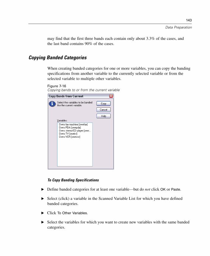
143

Data Preparation

may find that the first three bands each contain only about 3.3% of the cases, andthe last band contains 90% of the cases.

Copying Banded Categories

When creating banded categories for one or more variables, you can copy the bandingspecifications from another variable to the currently selected variable or from theselected variable to multiple other variables.

Figure 7-16Copying bands to or from the current variable

To Copy Banding Specifications

E Define banded categories for at least one variable—but do not click OK or Paste.

E Select (click) a variable in the Scanned Variable List for which you have definedbanded categories.

E Click To Other Variables.

E Select the variables for which you want to create new variables with the same bandedcategories.

144

Chapter 7

E Click Copy.

or

E Select (click) a variable in the Scanned Variable List to which you want to copydefined banded categories.

E Click From Another Variable.

E Select the variable with the defined banded categories that you want to copy.

E Click Copy.

If you have specified value labels for the variable from which you are copying thebanding specifications, those are also copied.

Note: Once you click OK in the Visual Bander main dialog box to create new bandedvariables (or close the dialog box in any other way), you cannot use the Visual Banderto copy those banded categories to other variables.

User-Missing Values in the Visual Bander

Values defined as user-missing (values identified as codes for missing data) forthe source variable are not included in the banded categories for the new variable.User-missing values for the source variables are copied as user-missing values for thenew variable, and any defined value labels for missing value codes are also copied.

If a missing value code conflicts with one of the banded category values for the newvariable, the missing value code for the new variable is recoded to a nonconflictingvalue by adding 100 to the highest banded category value. For example, if a value of 1is defined as user-missing for the source variable and the new variable will have sixbanded categories, any cases with a value of 1 for the source variable will have avalue of 106 for the new variable, and 106 will be defined as user-missing. If theuser-missing value for the source variable had a defined value label, that label will beretained as the value label for the recoded value of the new variable.

Note: If the source variable has a defined range of user-missing values of the formLO-n, where n is a positive number, the corresponding user-missing values for thenew variable will be negative numbers.

Chapter

8Data Transformations

In an ideal situation, your raw data are perfectly suitable for the type of analysis youwant to perform, and any relationships between variables are either conveniently linearor neatly orthogonal. Unfortunately, this is rarely the case. Preliminary analysis mayreveal inconvenient coding schemes or coding errors, or data transformations may berequired in order to expose the true relationship between variables.

You can perform data transformations ranging from simple tasks, such as collapsingcategories for analysis, to more advanced tasks, such as creating new variables basedon complex equations and conditional statements.

Computing Variables

Use the Compute dialog box to compute values for a variable based on numerictransformations of other variables.

You can compute values for numeric or string (alphanumeric) variables.

You can create new variables or replace the values of existing variables. For newvariables, you can also specify the variable type and label.

You can compute values selectively for subsets of data based on logical conditions.

You can use more than 70 built-in functions, including arithmetic functions,statistical functions, distribution functions, and string functions.

145

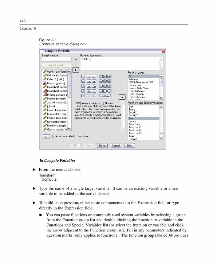
146

Chapter 8

Figure 8-1Compute Variable dialog box

To Compute Variables

E From the menus choose:Transform

Compute...

E Type the name of a single target variable. It can be an existing variable or a newvariable to be added to the active dataset.

E To build an expression, either paste components into the Expression field or typedirectly in the Expression field.

You can paste functions or commonly used system variables by selecting a groupfrom the Function group list and double-clicking the function or variable in theFunctions and Special Variables list (or select the function or variable and clickthe arrow adjacent to the Function group list). Fill in any parameters indicated byquestion marks (only applies to functions). The function group labeled All provides

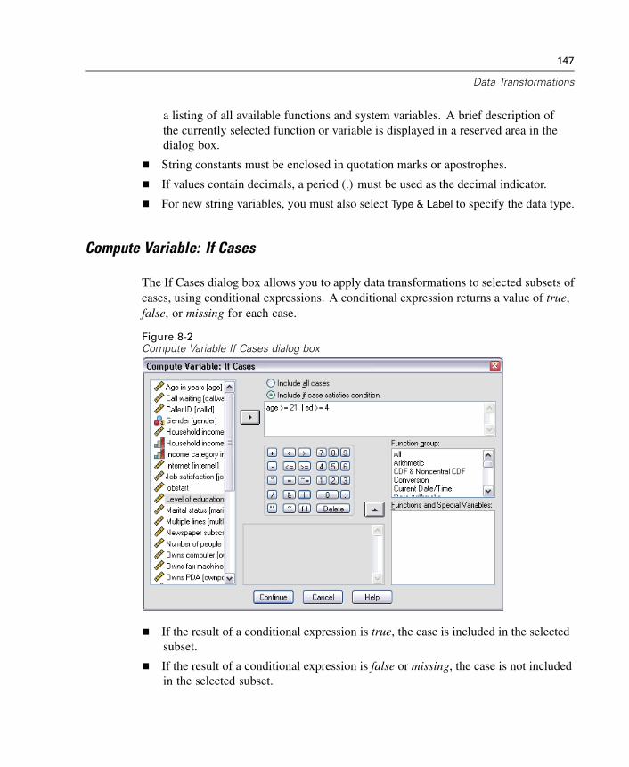
147

Data Transformations

a listing of all available functions and system variables. A brief description ofthe currently selected function or variable is displayed in a reserved area in thedialog box.

String constants must be enclosed in quotation marks or apostrophes.

If values contain decimals, a period (.) must be used as the decimal indicator.

For new string variables, you must also select Type & Label to specify the data type.

Compute Variable: If Cases

The If Cases dialog box allows you to apply data transformations to selected subsets ofcases, using conditional expressions. A conditional expression returns a value of true,false, or missing for each case.

Figure 8-2Compute Variable If Cases dialog box

If the result of a conditional expression is true, the case is included in the selectedsubset.

If the result of a conditional expression is false or missing, the case is not includedin the selected subset.

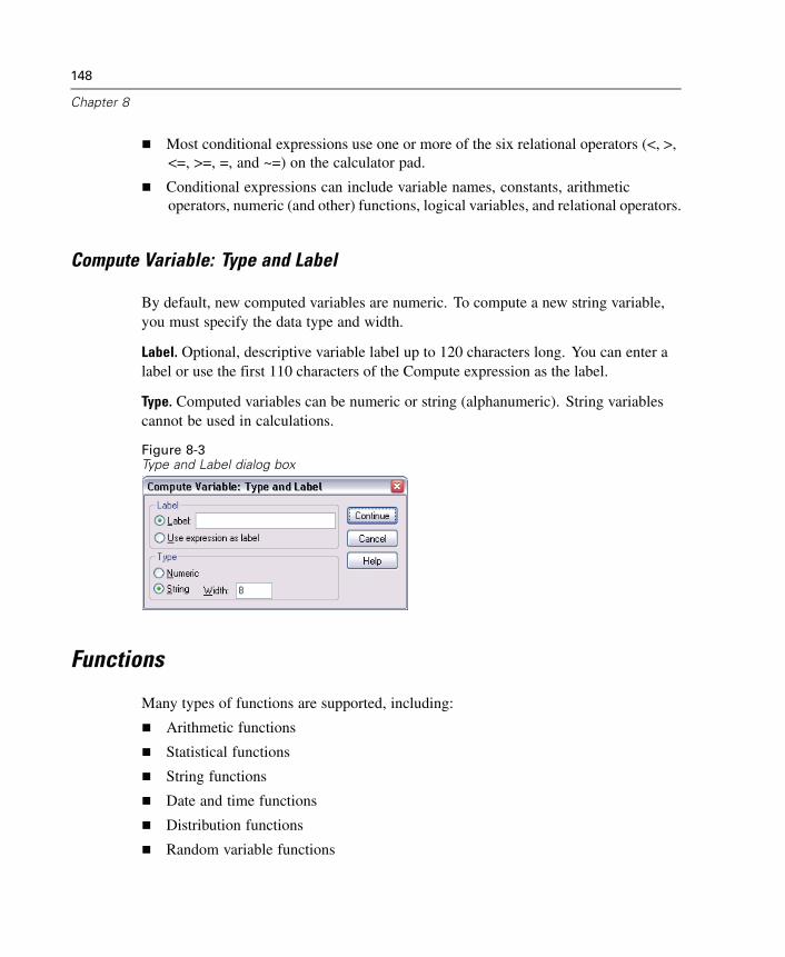
148

Chapter 8

Most conditional expressions use one or more of the six relational operators (<, >,<=, >=, =, and ~=) on the calculator pad.

Conditional expressions can include variable names, constants, arithmeticoperators, numeric (and other) functions, logical variables, and relational operators.

Compute Variable: Type and Label

By default, new computed variables are numeric. To compute a new string variable,you must specify the data type and width.

Label. Optional, descriptive variable label up to 120 characters long. You can enter alabel or use the first 110 characters of the Compute expression as the label.

Type. Computed variables can be numeric or string (alphanumeric). String variablescannot be used in calculations.

Figure 8-3Type and Label dialog box

Functions

Many types of functions are supported, including:

Arithmetic functions

Statistical functions

String functions

Date and time functions

Distribution functions

Random variable functions

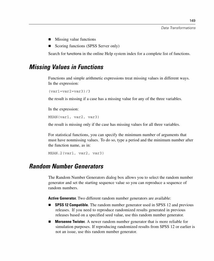
149


Missing value functions

Scoring functions (SPSS Server only)

Search for functions in the online Help system index for a complete list of functions.

Missing Values in Functions

Functions and simple arithmetic expressions treat missing values in different ways.In the expression:

(var1+var2+var3)/3

the result is missing if a case has a missing value for any of the three variables.

In the expression:

MEAN(var1, var2, var3)

the result is missing only if the case has missing values for all three variables.

For statistical functions, you can specify the minimum number of arguments thatmust have nonmissing values. To do so, type a period and the minimum number afterthe function name, as in:

MEAN.2(var1, var2, var3)

Random Number Generators

The Random Number Generators dialog box allows you to select the random numbergenerator and set the starting sequence value so you can reproduce a sequence ofrandom numbers.

Active Generator. Two different random number generators are available:

SPSS 12 Compatible. The random number generator used in SPSS 12 and previousreleases. If you need to reproduce randomized results generated in previousreleases based on a specified seed value, use this random number generator.

Mersenne Twister. A newer random number generator that is more reliable forsimulation purposes. If reproducing randomized results from SPSS 12 or earlier isnot an issue, use this random number generator.

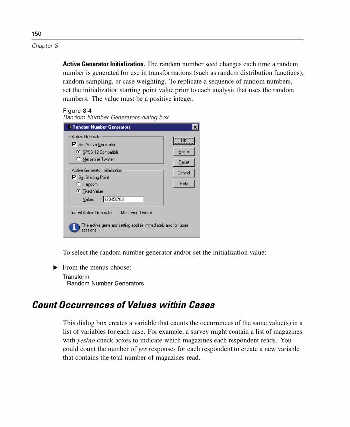
150

Chapter 8

Active Generator Initialization. The random number seed changes each time a randomnumber is generated for use in transformations (such as random distribution functions),random sampling, or case weighting. To replicate a sequence of random numbers,set the initialization starting point value prior to each analysis that uses the randomnumbers. The value must be a positive integer.

Figure 8-4Random Number Generators dialog box

To select the random number generator and/or set the initialization value:


Random Number Generators

Count Occurrences of Values within Cases

This dialog box creates a variable that counts the occurrences of the same value(s) in alist of variables for each case. For example, a survey might contain a list of magazineswith yes/no check boxes to indicate which magazines each respondent reads. Youcould count the number of yes responses for each respondent to create a new variablethat contains the total number of magazines read.

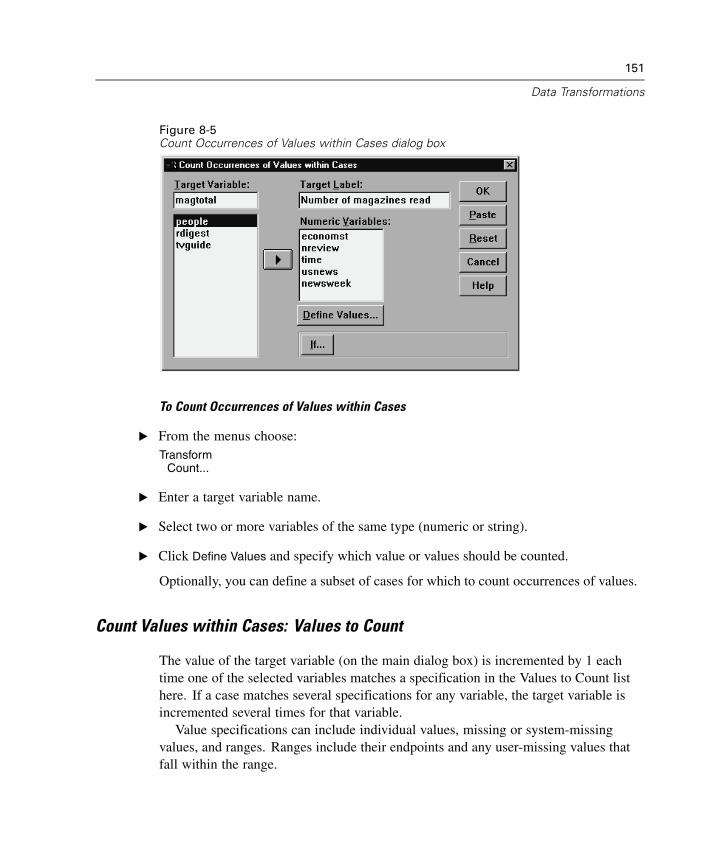
151


Figure 8-5Count Occurrences of Values within Cases dialog box

To Count Occurrences of Values within Cases


Count...

E Enter a target variable name.

E Select two or more variables of the same type (numeric or string).

E Click Define Values and specify which value or values should be counted.

Optionally, you can define a subset of cases for which to count occurrences of values.

Count Values within Cases: Values to Count

The value of the target variable (on the main dialog box) is incremented by 1 eachtime one of the selected variables matches a specification in the Values to Count listhere. If a case matches several specifications for any variable, the target variable isincremented several times for that variable.

Value specifications can include individual values, missing or system-missingvalues, and ranges. Ranges include their endpoints and any user-missing values thatfall within the range.

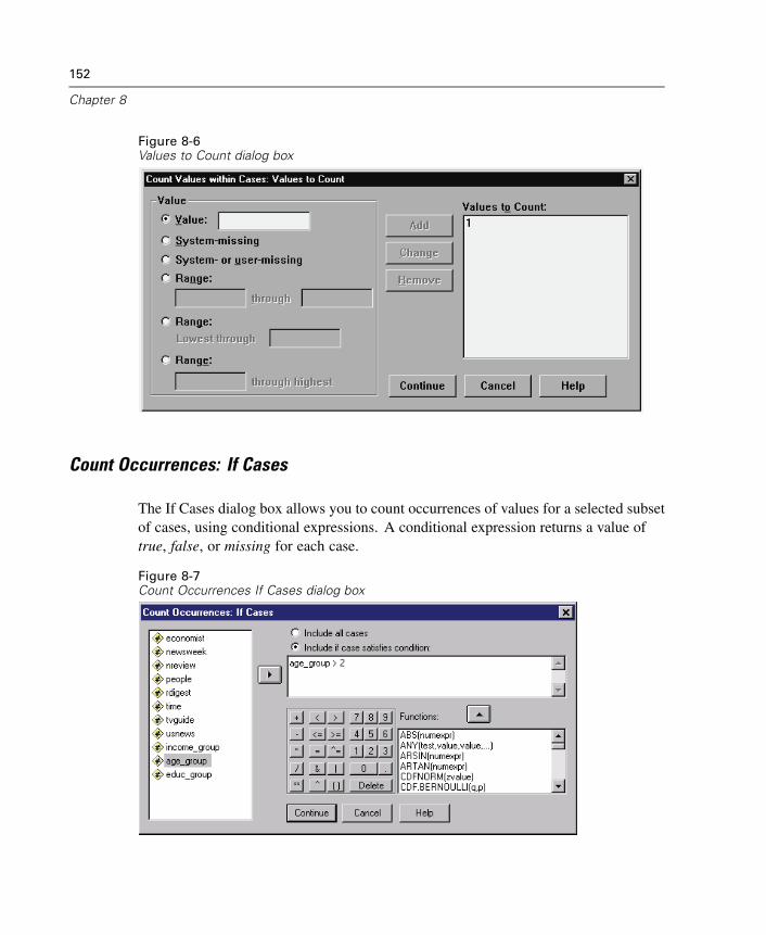
152

Chapter 8

Figure 8-6Values to Count dialog box

Count Occurrences: If Cases

The If Cases dialog box allows you to count occurrences of values for a selected subsetof cases, using conditional expressions. A conditional expression returns a value oftrue, false, or missing for each case.

Figure 8-7Count Occurrences If Cases dialog box

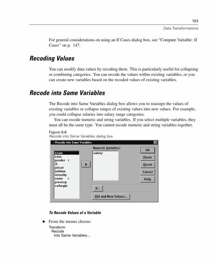
153


For general considerations on using an If Cases dialog box, see “Compute Variable: IfCases” on p. 147.

Recoding Values

You can modify data values by recoding them. This is particularly useful for collapsingor combining categories. You can recode the values within existing variables, or youcan create new variables based on the recoded values of existing variables.

Recode into Same Variables

The Recode into Same Variables dialog box allows you to reassign the values ofexisting variables or collapse ranges of existing values into new values. For example,you could collapse salaries into salary range categories.

You can recode numeric and string variables. If you select multiple variables, theymust all be the same type. You cannot recode numeric and string variables together.

Figure 8-8Recode into Same Variables dialog box

To Recode Values of a Variable


RecodeInto Same Variables...

154

Chapter 8

E Select the variables you want to recode. If you select multiple variables, they must bethe same type (numeric or string).

E Click Old and New Values and specify how to recode values.

Optionally, you can define a subset of cases to recode. The If Cases dialog box fordoing this is the same as the one described for Count Occurrences.

Recode into Same Variables: Old and New Values

You can define values to recode in this dialog box. All value specifications must be thesame data type (numeric or string) as the variables selected in the main dialog box.

Old Value. The value(s) to be recoded. You can recode single values, ranges of values,and missing values. System-missing values and ranges cannot be selected for stringvariables because neither concept applies to string variables. Ranges include theirendpoints and any user-missing values that fall within the range.

Value. Individual old value to be recoded into a new value. The value must be thesame data type (numeric or string) as the variable(s) being recoded.

System-missing. Values assigned by the program when values in your data areundefined according to the format type you have specified, when a numeric field isblank, or when a value resulting from a transformation command is undefined.Numeric system-missing values are displayed as periods. String variables cannothave system-missing values, since any character is legal in a string variable.

System- or user-missing. Observations with values that either have been defined asuser-missing values or are unknown and have been assigned the system-missingvalue, which is indicated with a period (.).

Range. Inclusive range of values. Not available for string variables. Anyuser-missing values within the range are included.

All other values. Any remaining values not included in one of the specifications onthe Old-New list. This appears as ELSE on the Old-New list.

New Value. The single value into which each old value or range of values is recoded.You can enter a value or assign the system-missing value.

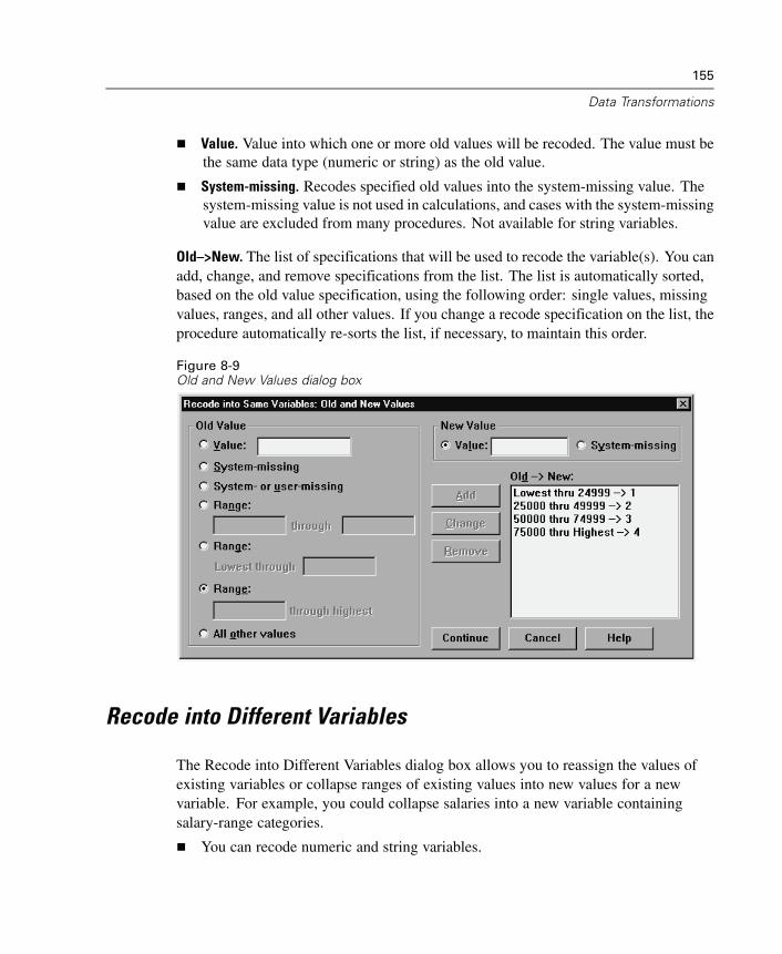
155


Value. Value into which one or more old values will be recoded. The value must bethe same data type (numeric or string) as the old value.

System-missing. Recodes specified old values into the system-missing value. Thesystem-missing value is not used in calculations, and cases with the system-missingvalue are excluded from many procedures. Not available for string variables.

Old–>New. The list of specifications that will be used to recode the variable(s). You canadd, change, and remove specifications from the list. The list is automatically sorted,based on the old value specification, using the following order: single values, missingvalues, ranges, and all other values. If you change a recode specification on the list, theprocedure automatically re-sorts the list, if necessary, to maintain this order.

Figure 8-9Old and New Values dialog box

Recode into Different Variables

The Recode into Different Variables dialog box allows you to reassign the values ofexisting variables or collapse ranges of existing values into new values for a newvariable. For example, you could collapse salaries into a new variable containingsalary-range categories.

You can recode numeric and string variables.

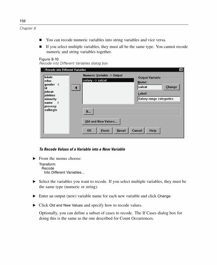
156

Chapter 8

You can recode numeric variables into string variables and vice versa.

If you select multiple variables, they must all be the same type. You cannot recodenumeric and string variables together.

Figure 8-10Recode into Different Variables dialog box

To Recode Values of a Variable into a New Variable


RecodeInto Different Variables...

E Select the variables you want to recode. If you select multiple variables, they must bethe same type (numeric or string).

E Enter an output (new) variable name for each new variable and click Change.

E Click Old and New Values and specify how to recode values.

Optionally, you can define a subset of cases to recode. The If Cases dialog box fordoing this is the same as the one described for Count Occurrences.

157


Recode into Different Variables: Old and New Values

You can define values to recode in this dialog box.

Old Value. The value(s) to be recoded. You can recode single values, ranges of values,and missing values. System-missing values and ranges cannot be selected for stringvariables because neither concept applies to string variables. Old values must be thesame data type (numeric or string) as the original variable. Ranges include theirendpoints and any user-missing values that fall within the range.

Value. Individual old value to be recoded into a new value. The value must be thesame data type (numeric or string) as the variable(s) being recoded.

System-missing. Values assigned by the program when values in your data areundefined according to the format type you have specified, when a numeric field isblank, or when a value resulting from a transformation command is undefined.Numeric system-missing values are displayed as periods. String variables cannothave system-missing values, since any character is legal in a string variable.

System- or user-missing. Observations with values that either have been defined asuser-missing values or are unknown and have been assigned the system-missingvalue, which is indicated with a period (.).

Range. Inclusive range of values. Not available for string variables. Anyuser-missing values within the range are included.

All other values. Any remaining values not included in one of the specifications onthe Old-New list. This appears as ELSE on the Old-New list.

New Value. The single value into which each old value or range of values is recoded.New values can be numeric or string.

Value. Value into which one or more old values will be recoded. The value must bethe same data type (numeric or string) as the old value.

System-missing. Recodes specified old values into the system-missing value. Thesystem-missing value is not used in calculations, and cases with the system-missingvalue are excluded from many procedures. Not available for string variables.

Copy old values. Retains the old value. If some values don't require recoding,use this to include the old values. Any old values that are not specified are notincluded in the new variable, and cases with those values will be assigned thesystem-missing value for the new variable.

Output variables are strings. Defines the new, recoded variable as a string(alphanumeric) variable. The old variable can be numeric or string.

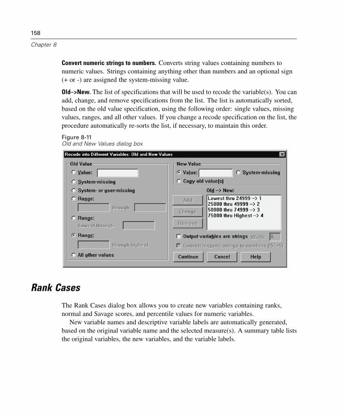
158

Chapter 8

Convert numeric strings to numbers. Converts string values containing numbers tonumeric values. Strings containing anything other than numbers and an optional sign(+ or -) are assigned the system-missing value.

Old–>New. The list of specifications that will be used to recode the variable(s). You canadd, change, and remove specifications from the list. The list is automatically sorted,based on the old value specification, using the following order: single values, missingvalues, ranges, and all other values. If you change a recode specification on the list, theprocedure automatically re-sorts the list, if necessary, to maintain this order.

Figure 8-11Old and New Values dialog box

Rank Cases

The Rank Cases dialog box allows you to create new variables containing ranks,normal and Savage scores, and percentile values for numeric variables.

New variable names and descriptive variable labels are automatically generated,based on the original variable name and the selected measure(s). A summary table liststhe original variables, the new variables, and the variable labels.

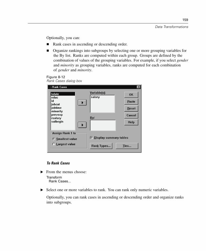
159



Rank cases in ascending or descending order.

Organize rankings into subgroups by selecting one or more grouping variables forthe By list. Ranks are computed within each group. Groups are defined by thecombination of values of the grouping variables. For example, if you select genderand minority as grouping variables, ranks are computed for each combinationof gender and minority.

Figure 8-12Rank Cases dialog box

To Rank Cases


Rank Cases...

E Select one or more variables to rank. You can rank only numeric variables.

Optionally, you can rank cases in ascending or descending order and organize ranksinto subgroups.

160

Chapter 8

Rank Cases: Types

You can select multiple ranking methods. A separate ranking variable is createdfor each method. Ranking methods include simple ranks, Savage scores, fractionalranks, and percentiles. You can also create rankings based on proportion estimatesand normal scores.

Rank. Simple rank. The value of the new variable equals its rank.

Savage score. The new variable contains Savage scores based on an exponentialdistribution.

Fractional rank. The value of the new variable equals rank divided by the sum of theweights of the nonmissing cases.

Fractional rank as percent. Each rank is divided by the number of cases with validvalues and multiplied by 100.

Sum of case weights. The value of the new variable equals the sum of case weights.The new variable is a constant for all cases in the same group.

Ntiles. Ranks are based on percentile groups, with each group containing approximatelythe same number of cases. For example, 4 Ntiles would assign a rank of 1 to casesbelow the 25th percentile, 2 to cases between the 25th and 50th percentile, 3 to casesbetween the 50th and 75th percentile, and 4 to cases above the 75th percentile.

Proportion estimates. Estimates of the cumulative proportion of the distributioncorresponding to a particular rank.

Normal scores. The z scores corresponding to the estimated cumulative proportion.

Proportion Estimation Formula. For proportion estimates and normal scores, you canselect the proportion estimation formula: Blom, Tukey, Rankit, or Van der Waerden.

Blom. Creates new ranking variable based on proportion estimates that uses theformula (r-3/8) / (w+1/4), where w is the sum of the case weights and r is the rank.

Tukey. Uses the formula (r-1/3) / (w+1/3), where r is the rank and w is the sum ofthe case weights.

Rankit. Uses the formula (r-1/2) / w, where w is the number of observations and r isthe rank, ranging from 1 to w.

Van der Waerden. Van der Waerden's transformation, defined by the formular/(w+1), where w is the sum of the case weights and r is the rank, ranging from 1to w.

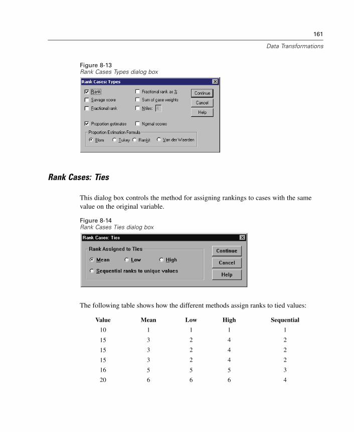
161


Figure 8-13Rank Cases Types dialog box

Rank Cases: Ties

This dialog box controls the method for assigning rankings to cases with the samevalue on the original variable.

Figure 8-14Rank Cases Ties dialog box

The following table shows how the different methods assign ranks to tied values:

Value Mean Low High Sequential

10 1 1 1 1

15 3 2 4 2

15 3 2 4 2

15 3 2 4 2

16 5 5 5 3

20 6 6 6 4

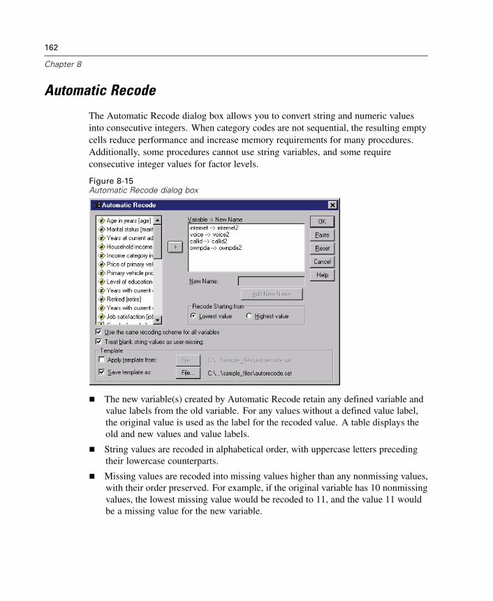
162

Chapter 8

Automatic Recode

The Automatic Recode dialog box allows you to convert string and numeric valuesinto consecutive integers. When category codes are not sequential, the resulting emptycells reduce performance and increase memory requirements for many procedures.Additionally, some procedures cannot use string variables, and some requireconsecutive integer values for factor levels.

Figure 8-15Automatic Recode dialog box

The new variable(s) created by Automatic Recode retain any defined variable andvalue labels from the old variable. For any values without a defined value label,the original value is used as the label for the recoded value. A table displays theold and new values and value labels.

String values are recoded in alphabetical order, with uppercase letters precedingtheir lowercase counterparts.

Missing values are recoded into missing values higher than any nonmissing values,with their order preserved. For example, if the original variable has 10 nonmissingvalues, the lowest missing value would be recoded to 11, and the value 11 wouldbe a missing value for the new variable.

163


Use the same recoding scheme for all variables. This option allows you to apply a singleautorecoding scheme to all the selected variables, yielding a consistent coding schemefor all the new variables.

If you select this option, the following rules and limitations apply:

All variables must be of the same type (numeric or string).

All observed values for all selected variables are used to create a sorted order ofvalues to recode into sequential integers.

User-missing values for the new variables are based on the first variable in the listwith defined user-missing values. All other values from other original variables,except for system-missing, are treated as valid.

Treat blank string values as user-missing. For string variables, blank or null valuesare not treated as system-missing. This option will autorecode blank strings into auser-missing value higher than the highest non-missing value.

Templates

You can save the autorecoding scheme in a template file and then apply it to othervariables and other data files.

For example, you may have a large number of alphanumeric product codes that youautorecode into integers every month, but some months new product codes are addedthat change the original autorecoding scheme. If you save the original scheme in atemplate and then apply it to the new data that contain the new set of codes, any newcodes encountered in the data are autorecoded into values higher that the last value inthe template, preserving the original autorecode scheme of the original product codes.

Save template as. Saves the autorecode scheme for the selected variables in an externaltemplate file.

The template contains information that maps the original non-missing values tothe recoded values.

Only information for non-missing values is saved in the template. User-missingvalue information is not retained.

164

Chapter 8

If you have selected multiple variables for recoding but you have not selected touse the same autorecoding scheme for all variables or you are not applying anexisting template as part of the autorecoding, the template will be based on thefirst variable in the list.

If you have selected multiple variables for recoding and you have also selected Usethe same recoding scheme for all variables and/or you have selected Apply template,then the template will contain the combined autorecoding scheme for all variables.

Apply template from. Applies a previously saved autorecode template to variablesselected for recoding, appending any additional values found in the variables to theend of the scheme, preserving the relationship between the original and autorecodedvalues stored in the saved scheme.

All variables selected for recoding must be the same type (numeric or string), andthat type must match the type defined in the template.

Templates do not contain any information on user-missing values. User-missingvalues for the target variables are based on the first variable in the originalvariable list with defined user-missing values. All other values from other originalvariables, except for system-missing, are treated as valid.

Value mappings from the template are applied first. All remaining values arerecoded into values higher than the last value in the template, with user-missingvalues (based on the first variable in the list with defined user-missing values)recoded into values higher than the last valid value.

If you have selected multiple variables for autorecoding, the template is appliedfirst, followed by a common, combined autorecoding for all additional valuesfound in the selected variables, resulting in a single, common autorecoding schemefor all selected variables.

To Recode String or Numeric Values into Consecutive Integers


Automatic Recode...

E Select one or more variables to recode.

E For each selected variable, enter a name for the new variable and click New Name.

165


Date and Time WizardThe Date and Time Wizard simplifies a number of common tasks associated withdate and time variables.

To Use the Date and Time Wizard


Date/Time...

E Select the task you wish to accomplish and follow the steps to define the task.

Figure 8-16Date and Time Wizard introduction screen

Learn how dates and times are represented in SPSS. This choice leads to a screenthat provides a brief overview of date/time variables in SPSS. By clicking on theHelp button, it also provides a link to more detailed information.

Create a date/time variable from a string containing a date or time. Use this optionto create a date/time variable from a string variable. For example, you have astring variable representing dates in the form mm/dd/yyyy and want to create adate/time variable from this.

166

Chapter 8

Create a date/time variable from variables holding parts of dates or times. This choiceallows you to construct a date/time variable from a set of existing variables. Forexample, you have a variable that represents the month (as an integer), a secondthat represents the day of the month, and a third that represents the year. You cancombine these three variables into a single date/time variable.

Calculate with dates and times. Use this option to add or subtract values fromdate/time variables. For example, you can calculate the duration of a processby subtracting a variable representing the start time of the process from anothervariable representing the end time of the process.

Extract a part of a date or time variable. This option allows you to extract part of adate/time variable, such as the day of the month from a date/time variable, whichhas the form mm/dd/yyyy.

Assign periodicity to a dataset. This choice takes you to the Define Dates dialogbox, used to create date/time variables that consist of a set of sequential dates. Thisfeature is typically used to associate dates with time series data.

Note: Tasks are disabled when the dataset lacks the types of variables required toaccomplish the task. For instance, if the dataset contains no string variables, then thetask to create a date/time variable from a string does not apply and is disabled.

Dates and Times in SPSS

Variables that represent dates and times in SPSS have a variable type of numeric, withdisplay formats that correspond to the specific date/time formats. These variables aregenerally referred to as date/time variables. SPSS distinguishes between date/timevariables that actually represent dates and those that represent a time duration that isindependent of any date, such as 20 hours, 10 minutes and 15 seconds. The latter arereferred to as duration variables and the former as date or date/time variables. For acomplete list of display formats, see “Date and Time” in the “Universals” section ofthe SPSS Command Syntax Reference.

Date and date/time variables. Date variables have a format representing a date, suchas mm/dd/yyyy. Date/time variables have a format representing a date and time, suchas dd-mmm-yyyy hh:mm:ss. Internally, date and date/time variables are stored as thenumber of seconds from October 14, 1582. Date and date/time variables are sometimesreferred to as date-format variables.

167


Both two- and four-digit year specifications are recognized. By default, two-digityears represent a range beginning 69 years prior to the current date and ending 30years after the current date. This range is determined by your Options settings andis configurable (from the Edit menu, choose Options and click the Data tab).

Dashes, periods, commas, slashes, or blanks can be used as delimiters inday-month-year formats.

Months can be represented in digits, Roman numerals, or three-characterabbreviations, and they can be fully spelled out. Three-letter abbreviationsand fully spelled-out month names must be in English; month names in otherlanguages are not recognized.

Duration Variables. Duration variables have a format representing a time duration, suchas hh:mm. They are stored internally as seconds without reference to a particular date.

In time specifications (applies to date/time and duration variables), colons can beused as delimiters between hours, minutes, and seconds. Hours and minutes arerequired, but seconds are optional. A period is required to separate seconds fromfractional seconds. Hours can be of unlimited magnitude, but the maximum valuefor minutes is 59 and for seconds is 59.999....

Current Date and Time. The system variable $TIME holds the current date and time. Itrepresents the number of seconds from October 14, 1582, to the date and time whenthe transformation command that uses it is executed.

Create a Date/Time Variable from a String

To create a date/time variable from a string variable:

E Select Create a date/time variable from a string containing a date or time on theintroduction screen of the Date and Time Wizard.

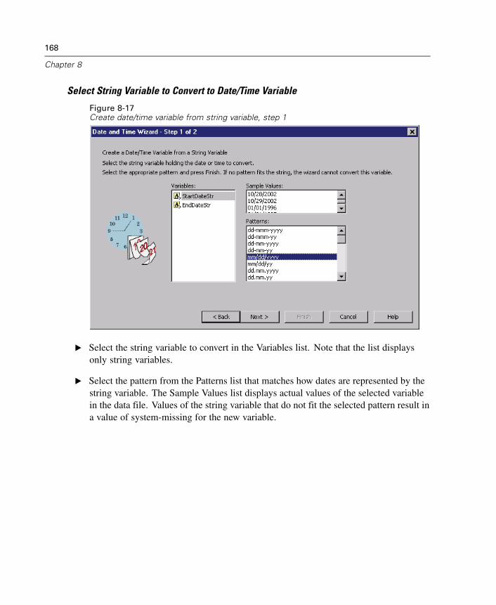
168

Chapter 8

Select String Variable to Convert to Date/Time Variable

Figure 8-17Create date/time variable from string variable, step 1

E Select the string variable to convert in the Variables list. Note that the list displaysonly string variables.

E Select the pattern from the Patterns list that matches how dates are represented by thestring variable. The Sample Values list displays actual values of the selected variablein the data file. Values of the string variable that do not fit the selected pattern result ina value of system-missing for the new variable.

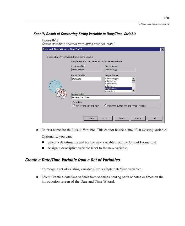
169


Specify Result of Converting String Variable to Date/Time Variable

Figure 8-18Create date/time variable from string variable, step 2

E Enter a name for the Result Variable. This cannot be the name of an existing variable.


Select a date/time format for the new variable from the Output Format list.

Assign a descriptive variable label to the new variable.

Create a Date/Time Variable from a Set of Variables

To merge a set of existing variables into a single date/time variable:

E Select Create a date/time variable from variables holding parts of dates or times on theintroduction screen of the Date and Time Wizard.

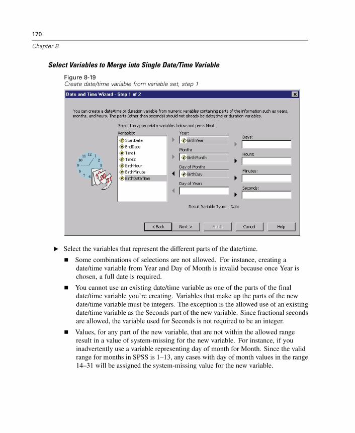
170

Chapter 8

Select Variables to Merge into Single Date/Time Variable

Figure 8-19Create date/time variable from variable set, step 1

E Select the variables that represent the different parts of the date/time.

Some combinations of selections are not allowed. For instance, creating adate/time variable from Year and Day of Month is invalid because once Year ischosen, a full date is required.

You cannot use an existing date/time variable as one of the parts of the finaldate/time variable you’re creating. Variables that make up the parts of the newdate/time variable must be integers. The exception is the allowed use of an existingdate/time variable as the Seconds part of the new variable. Since fractional secondsare allowed, the variable used for Seconds is not required to be an integer.

Values, for any part of the new variable, that are not within the allowed rangeresult in a value of system-missing for the new variable. For instance, if youinadvertently use a variable representing day of month for Month. Since the validrange for months in SPSS is 1–13, any cases with day of month values in the range14–31 will be assigned the system-missing value for the new variable.

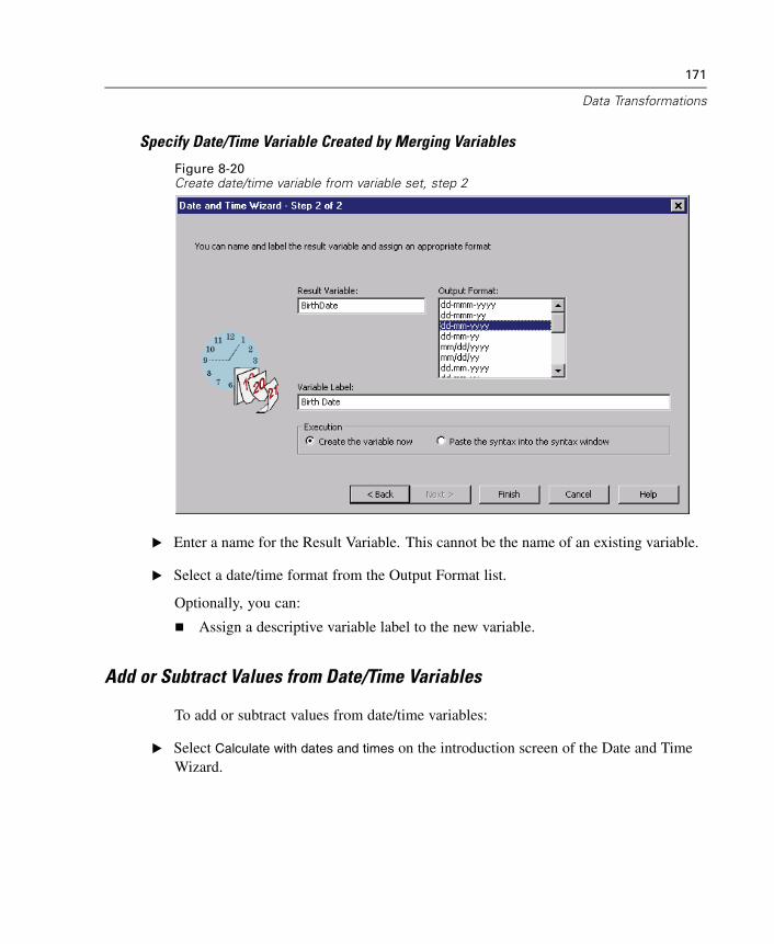
171


Specify Date/Time Variable Created by Merging Variables

Figure 8-20Create date/time variable from variable set, step 2

E Enter a name for the Result Variable. This cannot be the name of an existing variable.

E Select a date/time format from the Output Format list.



Add or Subtract Values from Date/Time Variables

To add or subtract values from date/time variables:

E Select Calculate with dates and times on the introduction screen of the Date and TimeWizard.

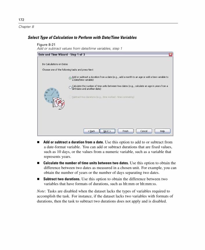
172

Chapter 8

Select Type of Calculation to Perform with Date/Time Variables

Figure 8-21Add or subtract values from date/time variables, step 1

Add or subtract a duration from a date. Use this option to add to or subtract froma date-format variable. You can add or subtract durations that are fixed values,such as 10 days, or the values from a numeric variable, such as a variable thatrepresents years.

Calculate the number of time units between two dates. Use this option to obtain thedifference between two dates as measured in a chosen unit. For example, you canobtain the number of years or the number of days separating two dates.

Subtract two durations. Use this option to obtain the difference between twovariables that have formats of durations, such as hh:mm or hh:mm:ss.

Note: Tasks are disabled when the dataset lacks the types of variables required toaccomplish the task. For instance, if the dataset lacks two variables with formats ofdurations, then the task to subtract two durations does not apply and is disabled.

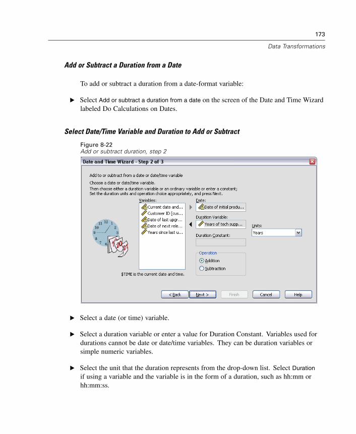
173


Add or Subtract a Duration from a Date

To add or subtract a duration from a date-format variable:

E Select Add or subtract a duration from a date on the screen of the Date and Time Wizardlabeled Do Calculations on Dates.

Select Date/Time Variable and Duration to Add or Subtract

Figure 8-22Add or subtract duration, step 2

E Select a date (or time) variable.

E Select a duration variable or enter a value for Duration Constant. Variables used fordurations cannot be date or date/time variables. They can be duration variables orsimple numeric variables.

E Select the unit that the duration represents from the drop-down list. Select Duration

if using a variable and the variable is in the form of a duration, such as hh:mm orhh:mm:ss.

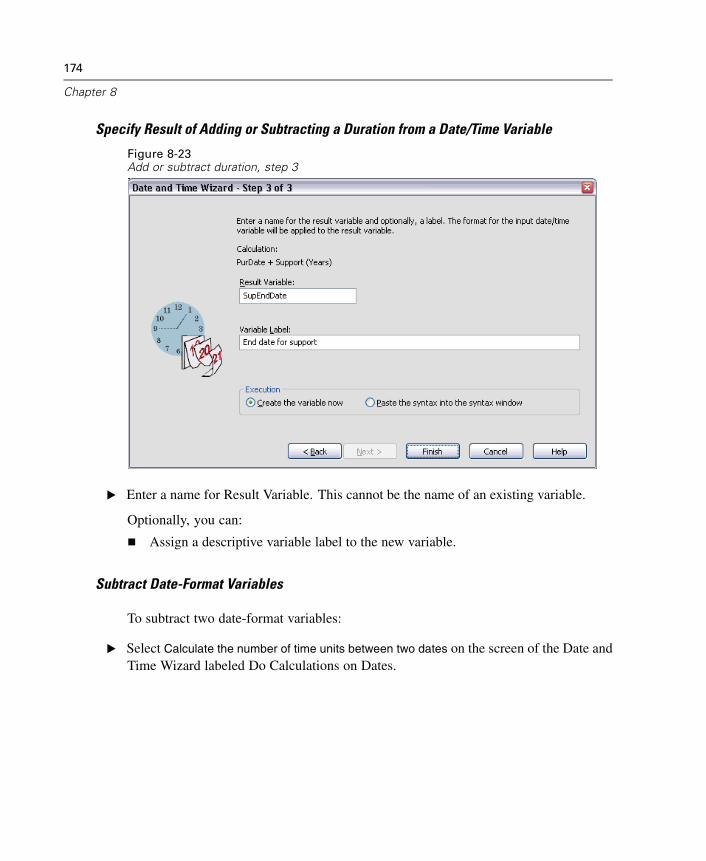
174

Chapter 8

Specify Result of Adding or Subtracting a Duration from a Date/Time Variable

Figure 8-23Add or subtract duration, step 3

E Enter a name for Result Variable. This cannot be the name of an existing variable.



Subtract Date-Format Variables

To subtract two date-format variables:

E Select Calculate the number of time units between two dates on the screen of the Date andTime Wizard labeled Do Calculations on Dates.

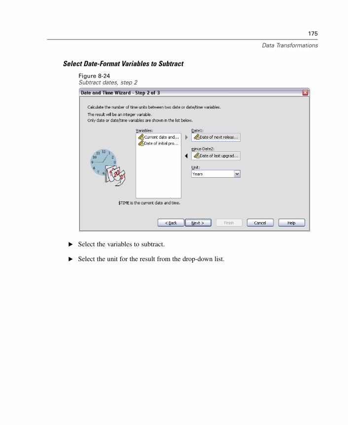
175


Select Date-Format Variables to Subtract

Figure 8-24Subtract dates, step 2

E Select the variables to subtract.

E Select the unit for the result from the drop-down list.

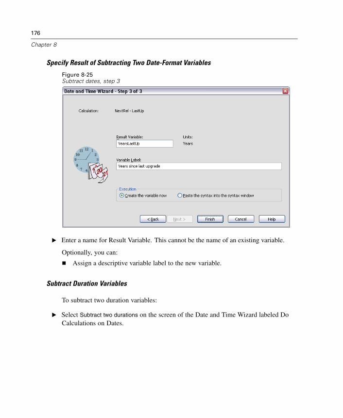
176

Chapter 8

Specify Result of Subtracting Two Date-Format Variables

Figure 8-25Subtract dates, step 3




Subtract Duration Variables

To subtract two duration variables:

E Select Subtract two durations on the screen of the Date and Time Wizard labeled DoCalculations on Dates.

177


Select Duration Variables to Subtract

Figure 8-26Subtract durations, step 2

E Select the variables to subtract.

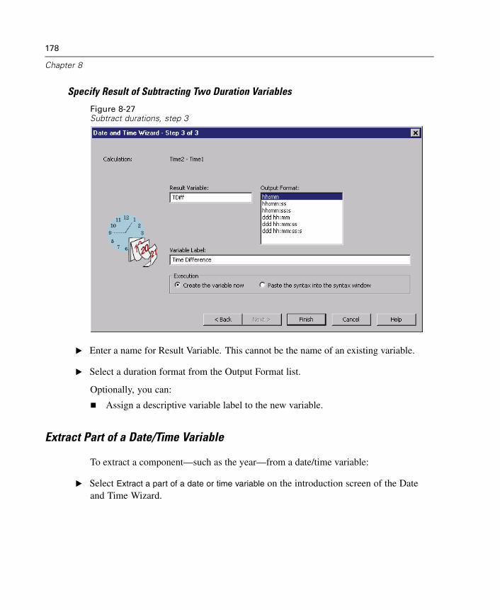
178

Chapter 8

Specify Result of Subtracting Two Duration Variables

Figure 8-27Subtract durations, step 3


E Select a duration format from the Output Format list.



Extract Part of a Date/Time Variable

To extract a component—such as the year—from a date/time variable:

E Select Extract a part of a date or time variable on the introduction screen of the Dateand Time Wizard.

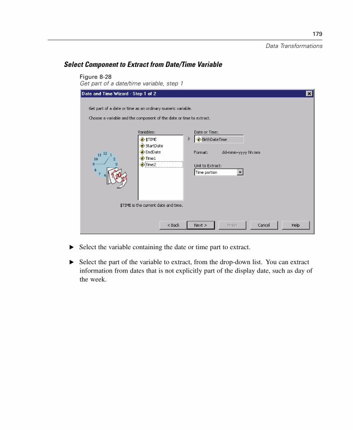
179


Select Component to Extract from Date/Time Variable

Figure 8-28Get part of a date/time variable, step 1

E Select the variable containing the date or time part to extract.

E Select the part of the variable to extract, from the drop-down list. You can extractinformation from dates that is not explicitly part of the display date, such as day ofthe week.

180

Chapter 8

Specify Result of Extracting Component from Date/Time Variable

Figure 8-29Get part of a date/time variable, step 2


E If you’re extracting the date or time part of a date/time variable, then you must select aformat from the Output Format list. In cases where the output format is not required,the Output Format list will be disabled.



Time Series Data Transformations

Several data transformations that are useful in time series analysis are provided:

Generate date variables to establish periodicity and to distinguish betweenhistorical, validation, and forecasting periods.

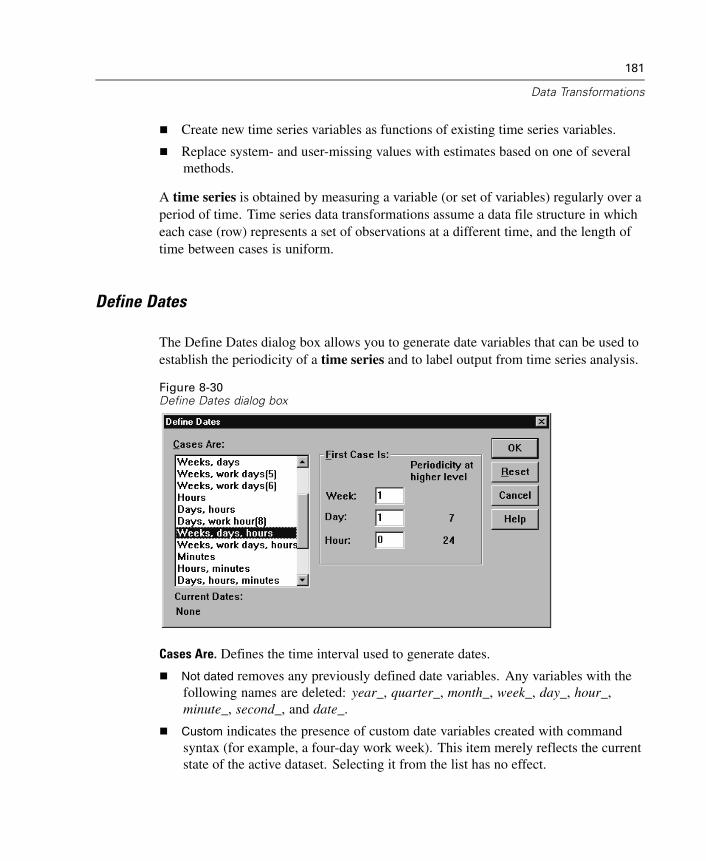
181


Create new time series variables as functions of existing time series variables.

Replace system- and user-missing values with estimates based on one of severalmethods.

A time series is obtained by measuring a variable (or set of variables) regularly over aperiod of time. Time series data transformations assume a data file structure in whicheach case (row) represents a set of observations at a different time, and the length oftime between cases is uniform.

Define Dates

The Define Dates dialog box allows you to generate date variables that can be used toestablish the periodicity of a time series and to label output from time series analysis.

Figure 8-30Define Dates dialog box

Cases Are. Defines the time interval used to generate dates.

Not dated removes any previously defined date variables. Any variables with thefollowing names are deleted: year_, quarter_, month_, week_, day_, hour_,minute_, second_, and date_.

Custom indicates the presence of custom date variables created with commandsyntax (for example, a four-day work week). This item merely reflects the currentstate of the active dataset. Selecting it from the list has no effect.

182

Chapter 8

First Case Is. Defines the starting date value, which is assigned to the first case.Sequential values, based on the time interval, are assigned to subsequent cases.

Periodicity at higher level. Indicates the repetitive cyclical variation, such as the numberof months in a year or the number of days in a week. The value displayed indicates themaximum value you can enter.

A new numeric variable is created for each component that is used to define the date.The new variable names end with an underscore. A descriptive string variable, date_,is also created from the components. For example, if you selected Weeks, days, hours,four new variables are created: week_, day_, hour_, and date_.

If date variables have already been defined, they are replaced when you define newdate variables that will have the same names as the existing date variables.

To Define Dates for Time Series Data


Define Dates...

E Select a time interval from the Cases Are list.

E Enter the value(s) that define the starting date for First Case Is, which determines thedate assigned to the first case.

Date Variables versus Date Format Variables

Date variables created with Define Dates should not be confused with date formatvariables, defined in the Variable view of the Data Editor. Date variables are usedto establish periodicity for time series data. Date format variables represent datesand/or times displayed in various date/time formats. Date variables are simple integersrepresenting the number of days, weeks, hours, and so on, from a user-specifiedstarting point. Internally, most date format variables are stored as the number ofseconds from October 14, 1582.

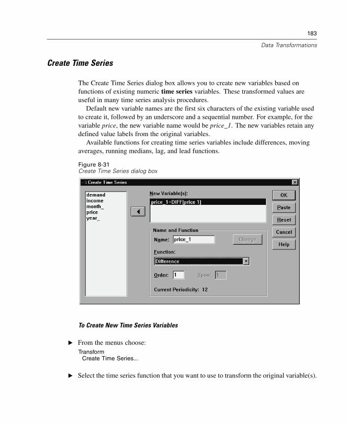
183


Create Time Series

The Create Time Series dialog box allows you to create new variables based onfunctions of existing numeric time series variables. These transformed values areuseful in many time series analysis procedures.

Default new variable names are the first six characters of the existing variable usedto create it, followed by an underscore and a sequential number. For example, for thevariable price, the new variable name would be price_1. The new variables retain anydefined value labels from the original variables.

Available functions for creating time series variables include differences, movingaverages, running medians, lag, and lead functions.

Figure 8-31Create Time Series dialog box

To Create New Time Series Variables


Create Time Series...

E Select the time series function that you want to use to transform the original variable(s).

184

Chapter 8

E Select the variable(s) from which you want to create new time series variables. Onlynumeric variables can be used.


Enter variable names to override the default new variable names.

Change the function for a selected variable.

Time Series Transformation Functions

Difference. Nonseasonal difference between successive values in the series. Theorder is the number of previous values used to calculate the difference. Because oneobservation is lost for each order of difference, system-missing values appear at thebeginning of the series. For example, if the difference order is 2, the first two caseswill have the system-missing value for the new variable.

Seasonal difference. Difference between series values a constant span apart. The spanis based on the currently defined periodicity. To compute seasonal differences, youmust have defined date variables (Data menu, Define Dates) that include a periodiccomponent (such as months of the year). The order is the number of seasonal periodsused to compute the difference. The number of cases with the system-missing valueat the beginning of the series is equal to the periodicity multiplied by the order. Forexample, if the current periodicity is 12 and the order is 2, the first 24 cases will havethe system-missing value for the new variable.

Centered moving average. Average of a span of series values surrounding and includingthe current value. The span is the number of series values used to compute theaverage. If the span is even, the moving average is computed by averaging each pairof uncentered means. The number of cases with the system-missing value at thebeginning and at the end of the series for a span of n is equal to n/2 for even spanvalues and for odd span values. For example, if the span is 5, the number of cases withthe system-missing value at the beginning and at the end of the series is 2.

Prior moving average. Average of the span of series values preceding the current value.The span is the number of preceding series values used to compute the average. Thenumber of cases with the system-missing value at the beginning of the series is equalto the span value.

Running median. Median of a span of series values surrounding and including thecurrent value. The span is the number of series values used to compute the median.If the span is even, the median is computed by averaging each pair of uncentered

185


medians. The number of cases with the system-missing value at the beginning and atthe end of the series for a span of n is equal to n/2 for even span values and for oddspan values. For example, if the span is 5, the number of cases with the system-missingvalue at the beginning and at the end of the series is 2.

Cumulative sum. Cumulative sum of series values up to and including the current value.

Lag. Value of a previous case, based on the specified lag order. The order is the numberof cases prior to the current case from which the value is obtained. The number of caseswith the system-missing value at the beginning of the series is equal to the order value.

Lead. Value of a subsequent case, based on the specified lead order. The order is thenumber of cases after the current case from which the value is obtained. The number ofcases with the system-missing value at the end of the series is equal to the order value.

Smoothing. New series values based on a compound data smoother. The smootherstarts with a running median of 4, which is centered by a running median of 2. It thenresmoothes these values by applying a running median of 5, a running median of 3,and hanning (running weighted averages). Residuals are computed by subtracting thesmoothed series from the original series. This whole process is then repeated on thecomputed residuals. Finally, the smoothed residuals are computed by subtractingthe smoothed values obtained the first time through the process. This is sometimesreferred to as T4253H smoothing.

Replace Missing Values

Missing observations can be problematic in analysis, and some time series measurescannot be computed if there are missing values in the series. Sometimes the value fora particular observation is simply not known. In addition, missing data can resultfrom any of the following:

Each degree of differencing reduces the length of a series by 1.

Each degree of seasonal differencing reduces the length of a series by one season.

If you create new series that contain forecasts beyond the end of the existing series(by clicking a Save button and making suitable choices), the original series and thegenerated residual series will have missing data for the new observations.

Some transformations (for example, the log transformation) produce missing datafor certain values of the original series.

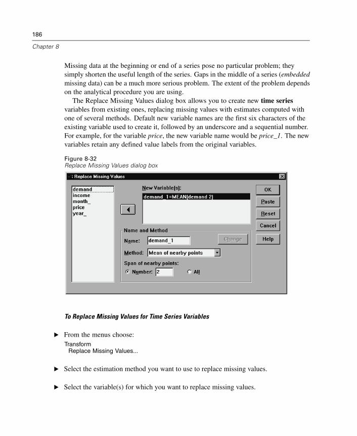
186

Chapter 8

Missing data at the beginning or end of a series pose no particular problem; theysimply shorten the useful length of the series. Gaps in the middle of a series (embeddedmissing data) can be a much more serious problem. The extent of the problem dependson the analytical procedure you are using.

The Replace Missing Values dialog box allows you to create new time seriesvariables from existing ones, replacing missing values with estimates computed withone of several methods. Default new variable names are the first six characters of theexisting variable used to create it, followed by an underscore and a sequential number.For example, for the variable price, the new variable name would be price_1. The newvariables retain any defined value labels from the original variables.

Figure 8-32Replace Missing Values dialog box

To Replace Missing Values for Time Series Variables


Replace Missing Values...

E Select the estimation method you want to use to replace missing values.

E Select the variable(s) for which you want to replace missing values.

187



Enter variable names to override the default new variable names.

Change the estimation method for a selected variable.

Estimation Methods for Replacing Missing Values

Series mean. Replaces missing values with the mean for the entire series.

Mean of nearby points. Replaces missing values with the mean of valid surroundingvalues. The span of nearby points is the number of valid values above and below themissing value used to compute the mean.

Median of nearby points. Replaces missing values with the median of valid surroundingvalues. The span of nearby points is the number of valid values above and below themissing value used to compute the median.

Linear interpolation. Replaces missing values using a linear interpolation. The last validvalue before the missing value and the first valid value after the missing value are usedfor the interpolation. If the first or last case in the series has a missing value, themissing value is not replaced.

Linear trend at point. Replaces missing values with the linear trend for that point. Theexisting series is regressed on an index variable scaled 1 to n. Missing values arereplaced with their predicted values.

Scoring Data with Predictive Models

The process of applying a predictive model to a set of data is referred to as scoringthe data. SPSS, Clementine, and AnswerTree have procedures for building predictivemodels such as regression, clustering, tree, and neural network models. Once a modelhas been built, the model specifications can be saved as an XML file containing all ofthe information necessary to reconstruct the model. The SPSS Server product thenprovides the means to read an XML model file and apply the model to a dataset.

Example. A credit application is rated for risk based on various aspects of the applicantand the loan in question. The credit score obtained from the risk model is used toaccept or reject the loan application.

188

Chapter 8

Scoring is treated as a transformation of the data. The model is expressed internally asa set of numeric transformations to be applied to a given set of variables—the predictorvariables specified in the model—in order to obtain a predicted result. In this sense,the process of scoring data with a given model is inherently the same as applying anyfunction, such as a square root function, to a set of data.

Scoring is only available with SPSS Server and can be done interactively by usersworking in distributed analysis mode. For scoring large data files you’ll probably wantto make use of the SPSS Batch Facility, a separate executable version of SPSS providedwith SPSS Server. For information about using the SPSS Batch Facility, see the SPSSBatch Facility User’s Guide, provided as a PDF file on the SPSS Server product CD.

The scoring process consists of the following:

E Loading a model from a file in XML (PMML) format.

E Computing your scores as a new variable, using the ApplyModel or StrApplyModelfunction available in the Compute Variable dialog.

For details concerning the ApplyModel or StrApplyModel function, see ScoringExpressions in the Transformation Expressions section of the SPSS Command SyntaxReference.

Loading a Saved Model

The Load Model dialog box allows you to load predictive models saved in XML(PMML) format, and is only available when working in distributed analysis mode.Loading models is a necessary first step to scoring data with them.

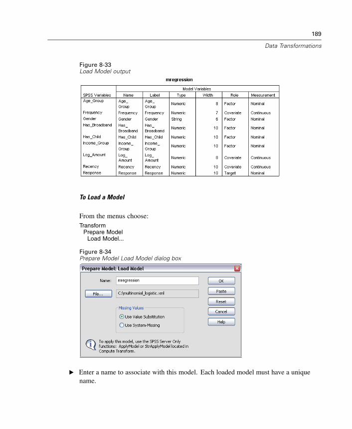
189


Figure 8-33Load Model output

To Load a Model

From the menus choose:Transform

Prepare ModelLoad Model...

Figure 8-34Prepare Model Load Model dialog box

E Enter a name to associate with this model. Each loaded model must have a uniquename.

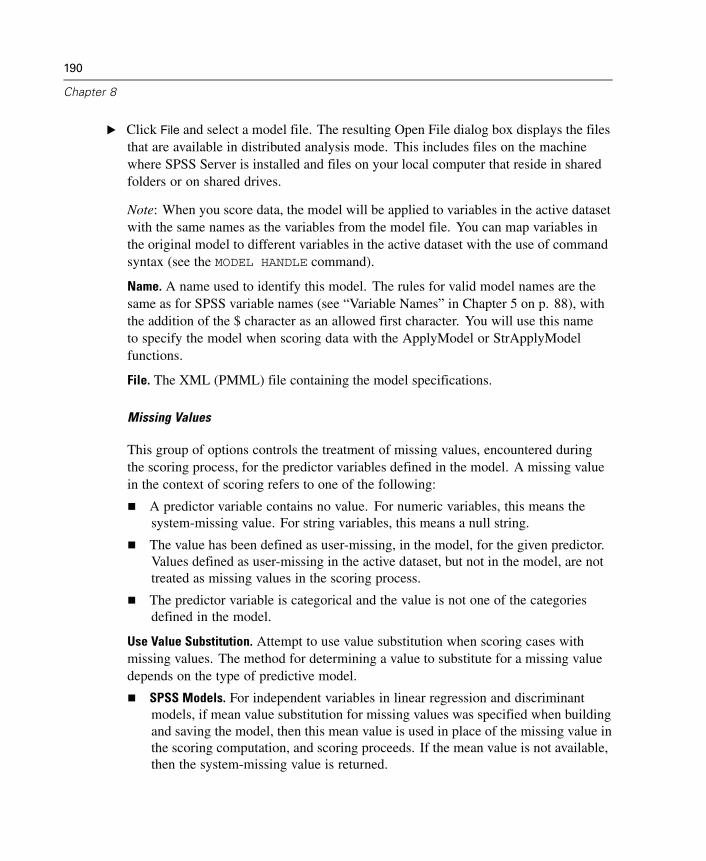
190

Chapter 8

E Click File and select a model file. The resulting Open File dialog box displays the filesthat are available in distributed analysis mode. This includes files on the machinewhere SPSS Server is installed and files on your local computer that reside in sharedfolders or on shared drives.

Note: When you score data, the model will be applied to variables in the active datasetwith the same names as the variables from the model file. You can map variables inthe original model to different variables in the active dataset with the use of commandsyntax (see the MODEL HANDLE command).

Name. A name used to identify this model. The rules for valid model names are thesame as for SPSS variable names (see “Variable Names” in Chapter 5 on p. 88), withthe addition of the $ character as an allowed first character. You will use this nameto specify the model when scoring data with the ApplyModel or StrApplyModelfunctions.

File. The XML (PMML) file containing the model specifications.

Missing Values

This group of options controls the treatment of missing values, encountered duringthe scoring process, for the predictor variables defined in the model. A missing valuein the context of scoring refers to one of the following:

A predictor variable contains no value. For numeric variables, this means thesystem-missing value. For string variables, this means a null string.

The value has been defined as user-missing, in the model, for the given predictor.Values defined as user-missing in the active dataset, but not in the model, are nottreated as missing values in the scoring process.

The predictor variable is categorical and the value is not one of the categoriesdefined in the model.

Use Value Substitution. Attempt to use value substitution when scoring cases withmissing values. The method for determining a value to substitute for a missing valuedepends on the type of predictive model.

SPSS Models. For independent variables in linear regression and discriminantmodels, if mean value substitution for missing values was specified when buildingand saving the model, then this mean value is used in place of the missing value inthe scoring computation, and scoring proceeds. If the mean value is not available,then the system-missing value is returned.

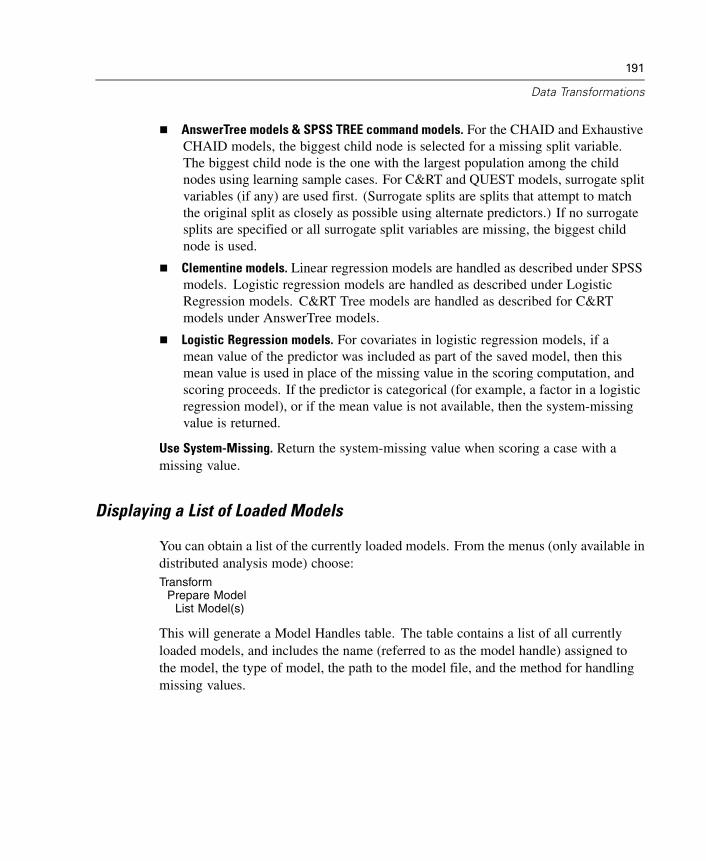
191


AnswerTree models & SPSS TREE command models. For the CHAID and ExhaustiveCHAID models, the biggest child node is selected for a missing split variable.The biggest child node is the one with the largest population among the childnodes using learning sample cases. For C&RT and QUEST models, surrogate splitvariables (if any) are used first. (Surrogate splits are splits that attempt to matchthe original split as closely as possible using alternate predictors.) If no surrogatesplits are specified or all surrogate split variables are missing, the biggest childnode is used.

Clementine models. Linear regression models are handled as described under SPSSmodels. Logistic regression models are handled as described under LogisticRegression models. C&RT Tree models are handled as described for C&RTmodels under AnswerTree models.

Logistic Regression models. For covariates in logistic regression models, if amean value of the predictor was included as part of the saved model, then thismean value is used in place of the missing value in the scoring computation, andscoring proceeds. If the predictor is categorical (for example, a factor in a logisticregression model), or if the mean value is not available, then the system-missingvalue is returned.

Use System-Missing. Return the system-missing value when scoring a case with amissing value.

Displaying a List of Loaded Models

You can obtain a list of the currently loaded models. From the menus (only available indistributed analysis mode) choose:Transform

Prepare ModelList Model(s)

This will generate a Model Handles table. The table contains a list of all currentlyloaded models, and includes the name (referred to as the model handle) assigned tothe model, the type of model, the path to the model file, and the method for handlingmissing values.

192

Chapter 8

Figure 8-35Listing of loaded models

Additional Features Available with Command Syntax

From the Load Model dialog box, you can paste your selections into a syntax windowand edit the resulting MODEL HANDLE command syntax. This allows you to:

Map variables in the original model to different variables in the active dataset (withthe MAP subcommand). By default, the model is applied to variables in the activedataset with the same names as the variables from the model file.

See the SPSS Command Syntax Reference for complete syntax information.

Chapter

9File Handling and FileTransformations

Data files are not always organized in the ideal form for your specific needs. Youmay want to combine data files, sort the data in a different order, select a subset ofcases, or change the unit of analysis by grouping cases together. A wide range of filetransformation capabilities is available, including the ability to:

Sort data. You can sort cases based on the value of one or more variables.

Transpose cases and variables. The SPSS data file format reads rows as cases andcolumns as variables. For data files in which this order is reversed, you can switch therows and columns and read the data in the correct format.

Merge files. You can merge two or more data files. You can combine files with thesame variables but different cases or the same cases but different variables.

Select subsets of cases. You can restrict your analysis to a subset of cases or performsimultaneous analyses on different subsets.

Aggregate data. You can change the unit of analysis by aggregating cases based on thevalue of one or more grouping variables.

Weight data. Weight cases for analysis based on the value of a weight variable.

Restructure data. You can restructure data to create a single case (record) from multiplecases or create multiple cases from a single case.

Sort Cases

This dialog box sorts cases (rows) of the data file based on the values of one or moresorting variables. You can sort cases in ascending or descending order.

193

194

Chapter 9

If you select multiple sort variables, cases are sorted by each variable withincategories of the preceding variable on the Sort list. For example, if you selectgender as the first sorting variable and minority as the second sorting variable,cases will be sorted by minority classification within each gender category.

For string variables, uppercase letters precede their lowercase counterparts in sortorder. For example, the string value “Yes” comes before “yes” in sort order.

Figure 9-1Sort Cases dialog box

To Sort Cases


Sort Cases...

E Select one or more sorting variables.

Transpose

Transpose creates a new data file in which the rows and columns in the original datafile are transposed so that cases (rows) become variables and variables (columns)become cases. Transpose automatically creates new variable names and displays alist of the new variable names.

A new string variable that contains the original variable name, case_lbl, isautomatically created.

195

File Handling and File Transformations

If the active dataset contains an ID or name variable with unique values, you canuse it as the name variable, and its values will be used as variable names in thetransposed data file. If it is a numeric variable, the variable names start with theletter V, followed by the numeric value.

User-missing values are converted to the system-missing value in the transposeddata file. To retain any of these values, change the definition of missing values inthe Variable view in the Data Editor.

To Transpose Variables and Cases


Transpose...

E Select one or more variables to transpose into cases.

Merging Data Files

You can merge data from two files in two different ways. You can:

Merge the active dataset with another open dataset or SPSS-format data filecontaining the same variables but different cases.

Merge the active dataset with another open dataset or SPSS-format data filecontaining the same cases but different variables.

To Merge Files


Merge Files

E Select Add Cases or Add Variables.

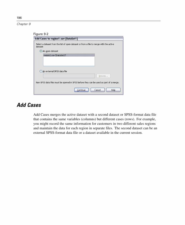
196

Chapter 9

Figure 9-2

Add Cases

Add Cases merges the active dataset with a second dataset or SPSS-format data filethat contains the same variables (columns) but different cases (rows). For example,you might record the same information for customers in two different sales regionsand maintain the data for each region in separate files. The second dataset can be anexternal SPSS-format data file or a dataset available in the current session.

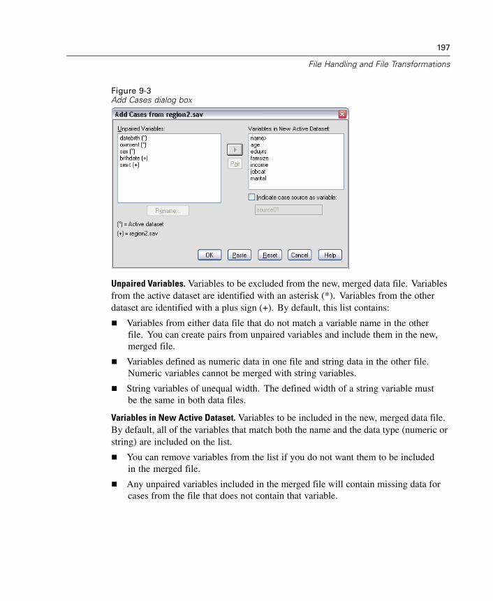
197


Figure 9-3Add Cases dialog box

Unpaired Variables. Variables to be excluded from the new, merged data file. Variablesfrom the active dataset are identified with an asterisk (*). Variables from the otherdataset are identified with a plus sign (+). By default, this list contains:

Variables from either data file that do not match a variable name in the otherfile. You can create pairs from unpaired variables and include them in the new,merged file.

Variables defined as numeric data in one file and string data in the other file.Numeric variables cannot be merged with string variables.

String variables of unequal width. The defined width of a string variable mustbe the same in both data files.

Variables in New Active Dataset. Variables to be included in the new, merged data file.By default, all of the variables that match both the name and the data type (numeric orstring) are included on the list.

You can remove variables from the list if you do not want them to be includedin the merged file.

Any unpaired variables included in the merged file will contain missing data forcases from the file that does not contain that variable.

198

Chapter 9

Indicate case source as variable. Indicates the source data file for each case. Thisvariable has a value of 0 for cases from the active dataset and a value of 1 for casesfrom the external data file.

To Merge Data Files with the Same Variables and Different Cases

E Open at least one of the data files that you want to merge. If you have multiple datasetsopen, make one of the datasets that you want to merge the active dataset. The casesfrom this file will appear first in the new, merged data file.


Merge FilesAdd Cases...

E Select the dataset or SPSS-format data file to merge with the active dataset.

E Remove any variables that you do not want from the Variables in New Active Datasetlist.

E Add any variable pairs from the Unpaired Variables list that represent the sameinformation recorded under different variable names in the two files. For example, dateof birth might have the variable name brthdate in one file and datebrth in the other file.

To Select a Pair of Unpaired Variables

E Click one of the variables on the Unpaired Variables list.

E Ctrl-click the other variable on the list. (Press the Ctrl key and click the left mousebutton at the same time.)

E Click Pair to move the variable pair to the Variables in New Active Dataset list. (Thevariable name from the active dataset is used as the variable name in the merged file.)

199


Figure 9-4Selecting pairs of variables with Ctrl-click

Add Cases: Rename

You can rename variables from either the active dataset or the other dataset beforemoving them from the unpaired list to the list of variables to be included in the mergeddata file. Renaming variables enables you to:

Use the variable name from the other dataset rather than the name from the activedataset for variable pairs.

Include two variables with the same name but of unmatched types or differentstring widths. For example, to include both the numeric variable sex from theactive dataset and the string variable sex from the other dataset, one of them mustbe renamed first.

200

Chapter 9

Add Cases: Dictionary Information

Any existing dictionary information (variable and value labels, user-missing values,display formats) in the active dataset is applied to the merged data file.

If any dictionary information for a variable is undefined in the active dataset,dictionary information from the other dataset is used.

If the active dataset contains any defined value labels or user-missing values fora variable, any additional value labels or user-missing values for that variable inthe other dataset are ignored.

Merging More Than Two Data Sources

Using command syntax, you can merge up to 50 datasets and/or data files. For moreinformation, see the ADD FILES command in the SPSS Command Syntax Reference(available from the Help menu).

Add Variables

Add Variables merges the active dataset with another open dataset or SPSS-formatdata file that contains the same cases (rows) but different variables (columns). Forexample, you might want to merge a data file that contains pre-test results with onethat contains post-test results.

Cases must be sorted in the same order in both datasets.

If one or more key variables are used to match cases, the two datasets must besorted by ascending order of the key variable(s).

Variable names in the second data file that duplicate variable names in the activedataset are excluded by default because Add Variables assumes that these variablescontain duplicate information.

Indicate case source as variable. Indicates the source data file for each case. Thisvariable has a value of 0 for cases from the active dataset and a value of 1 for casesfrom the external data file.

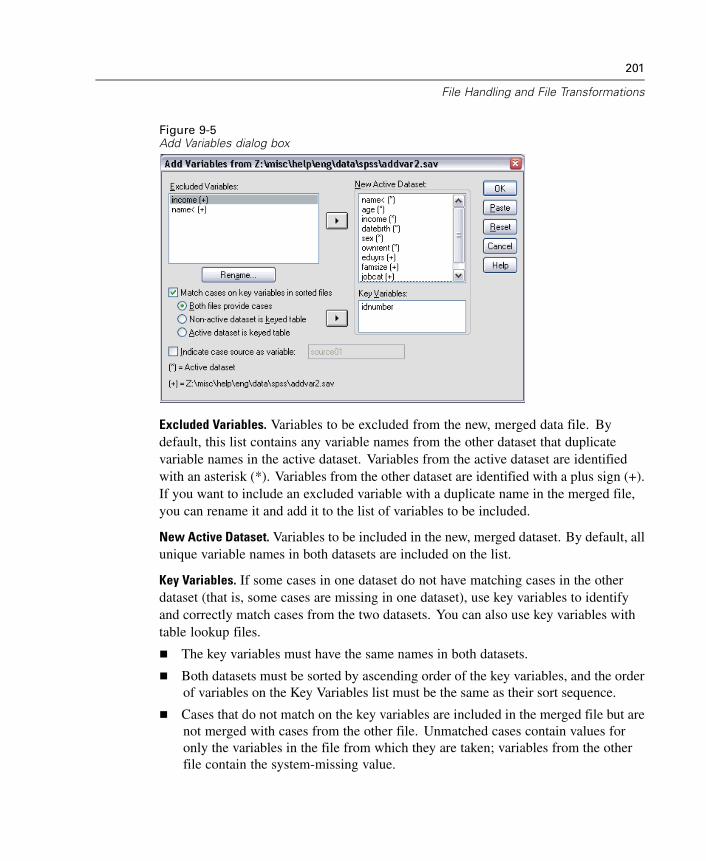
201


Figure 9-5Add Variables dialog box

Excluded Variables. Variables to be excluded from the new, merged data file. Bydefault, this list contains any variable names from the other dataset that duplicatevariable names in the active dataset. Variables from the active dataset are identifiedwith an asterisk (*). Variables from the other dataset are identified with a plus sign (+).If you want to include an excluded variable with a duplicate name in the merged file,you can rename it and add it to the list of variables to be included.

New Active Dataset. Variables to be included in the new, merged dataset. By default, allunique variable names in both datasets are included on the list.

Key Variables. If some cases in one dataset do not have matching cases in the otherdataset (that is, some cases are missing in one dataset), use key variables to identifyand correctly match cases from the two datasets. You can also use key variables withtable lookup files.

The key variables must have the same names in both datasets.

Both datasets must be sorted by ascending order of the key variables, and the orderof variables on the Key Variables list must be the same as their sort sequence.

Cases that do not match on the key variables are included in the merged file but arenot merged with cases from the other file. Unmatched cases contain values foronly the variables in the file from which they are taken; variables from the otherfile contain the system-missing value.

202

Chapter 9

Non-active or active dataset is keyed table. A keyed table, or table lookup file, is a filein which data for each “case” can be applied to multiple cases in the other data file.For example, if one file contains information on individual family members (suchas sex, age, education) and the other file contains overall family information (suchas total income, family size, location), you can use the file of family data as a tablelookup file and apply the common family data to each individual family memberin the merged data file.

To Merge Files with the Same Cases but Different Variables

E Open at least one of the data files that you want to merge. If you have multiple datasetsopen, make one of the datasets that you want to merge the active dataset.


Merge FilesAdd Variables...

E Select the dataset or SPSS-format data file to merge with the active dataset.

To Select Key Variables

E Select the variables from the external file variables (+) on the Excluded Variables list.

E Select Match cases on key variables in sorted files.

E Add the variables to the Key Variables list.

The key variables must exist in both the active dataset and the other dataset. Bothdatasets must be sorted by ascending order of the key variables, and the order ofvariables on the Key Variables list must be the same as their sort sequence.

Add Variables: Rename

You can rename variables from either the active dataset or the other dataset beforemoving them to the list of variables to be included in the merged data file. This isprimarily useful if you want to include two variables with the same name that containdifferent information in the two files.

203


Merging More Than Two Data Sources

Using command syntax, you can merge up to 50 datasets and/or data files. For moreinformation, see the MATCH FILES command in the SPSS Command Syntax Reference(available from the Help menu).

Aggregate Data

Aggregate Data aggregates groups of cases in the active dataset into single casesand creates a new, aggregated file or creates new variables in the active dataset thatcontain aggregated data. Cases are aggregated based on the value of one or morebreak (grouping) variables.

If you create a new, aggregated data file, the new data file contains one case foreach group defined by the break variables. For example, if there is one breakvariable with two values, the new data file will contain only two cases.

If you add aggregate variables to the active dataset, the data file itself is notaggregated. Each case with the same value(s) of the break variable(s) receivesthe same values for the new aggregate variables. For example, if gender is theonly break variable, all males would receive the same value for a new aggregatevariable that represents average age.

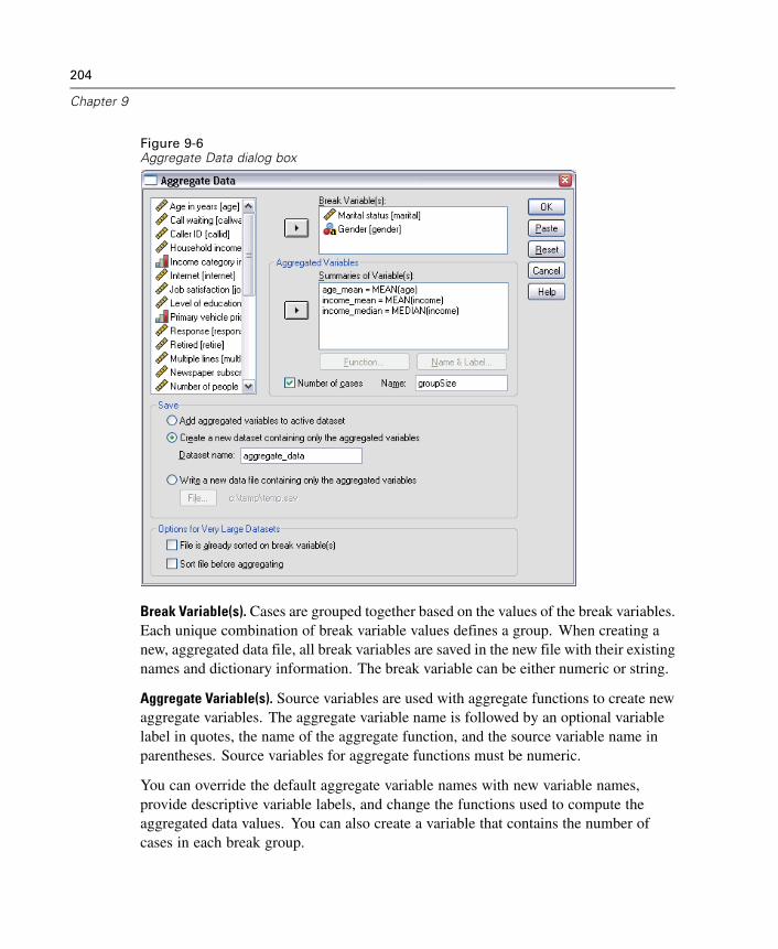
204

Chapter 9

Figure 9-6Aggregate Data dialog box

Break Variable(s). Cases are grouped together based on the values of the break variables.Each unique combination of break variable values defines a group. When creating anew, aggregated data file, all break variables are saved in the new file with their existingnames and dictionary information. The break variable can be either numeric or string.

Aggregate Variable(s). Source variables are used with aggregate functions to create newaggregate variables. The aggregate variable name is followed by an optional variablelabel in quotes, the name of the aggregate function, and the source variable name inparentheses. Source variables for aggregate functions must be numeric.

You can override the default aggregate variable names with new variable names,provide descriptive variable labels, and change the functions used to compute theaggregated data values. You can also create a variable that contains the number ofcases in each break group.

205


To Aggregate a Data File


Aggregate...

E Select one or more break variables that define how cases are grouped to createaggregated data.

E Select one or more aggregate variables.

E Select an aggregate function for each aggregate variable.

Saving Aggregated Results

You can add aggregate variables to the active dataset or create a new, aggregateddata file.

Add aggregated variables to active dataset. New variables based on aggregatefunctions are added to the active dataset. The data file itself is not aggregated.Each case with the same value(s) of the break variable(s) receives the same valuesfor the new aggregate variables.

Create a new dataset containing only the aggregated variables. Saves aggregateddata to a new dataset in the current session. The dataset includes the breakvariables that define the aggregated cases and all aggregate variables defined byaggregate functions. The active dataset is unaffected.

Write a new data file containing only the aggregated variables. Saves aggregateddata to an external data file. The file includes the break variables that define theaggregated cases and all aggregate variables defined by aggregate functions. Theactive dataset is unaffected.

Sorting Options for Large Data Files

For very large data files, it may be more efficient to aggregate presorted data.

File is already sorted on break variable(s). If the data have already been sorted by valuesof the break variables, this option enables the procedure to run more quickly and useless memory. Use this option with caution.

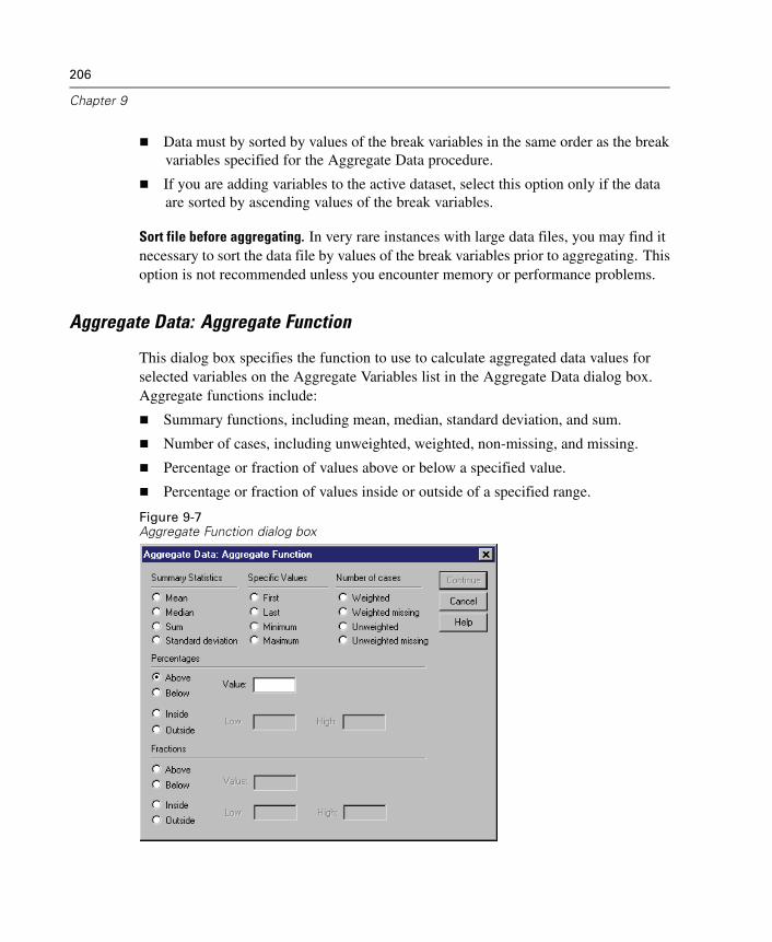
206

Chapter 9

Data must by sorted by values of the break variables in the same order as the breakvariables specified for the Aggregate Data procedure.

If you are adding variables to the active dataset, select this option only if the dataare sorted by ascending values of the break variables.

Sort file before aggregating. In very rare instances with large data files, you may find itnecessary to sort the data file by values of the break variables prior to aggregating. Thisoption is not recommended unless you encounter memory or performance problems.

Aggregate Data: Aggregate Function

This dialog box specifies the function to use to calculate aggregated data values forselected variables on the Aggregate Variables list in the Aggregate Data dialog box.Aggregate functions include:

Summary functions, including mean, median, standard deviation, and sum.

Number of cases, including unweighted, weighted, non-missing, and missing.

Percentage or fraction of values above or below a specified value.

Percentage or fraction of values inside or outside of a specified range.

Figure 9-7Aggregate Function dialog box

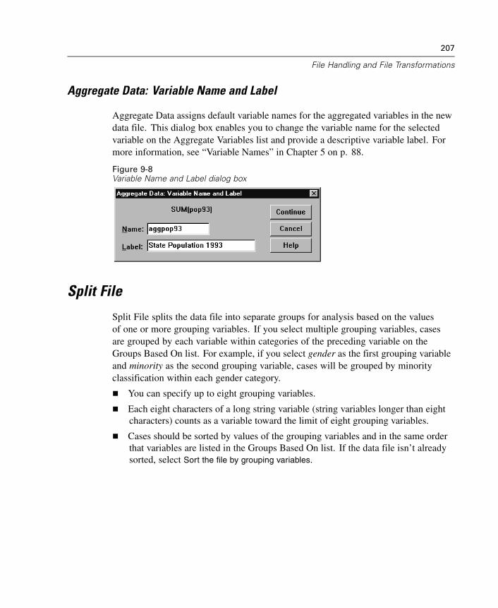
207


Aggregate Data: Variable Name and Label

Aggregate Data assigns default variable names for the aggregated variables in the newdata file. This dialog box enables you to change the variable name for the selectedvariable on the Aggregate Variables list and provide a descriptive variable label. Formore information, see “Variable Names” in Chapter 5 on p. 88.

Figure 9-8Variable Name and Label dialog box

Split File

Split File splits the data file into separate groups for analysis based on the valuesof one or more grouping variables. If you select multiple grouping variables, casesare grouped by each variable within categories of the preceding variable on theGroups Based On list. For example, if you select gender as the first grouping variableand minority as the second grouping variable, cases will be grouped by minorityclassification within each gender category.

You can specify up to eight grouping variables.

Each eight characters of a long string variable (string variables longer than eightcharacters) counts as a variable toward the limit of eight grouping variables.

Cases should be sorted by values of the grouping variables and in the same orderthat variables are listed in the Groups Based On list. If the data file isn’t alreadysorted, select Sort the file by grouping variables.

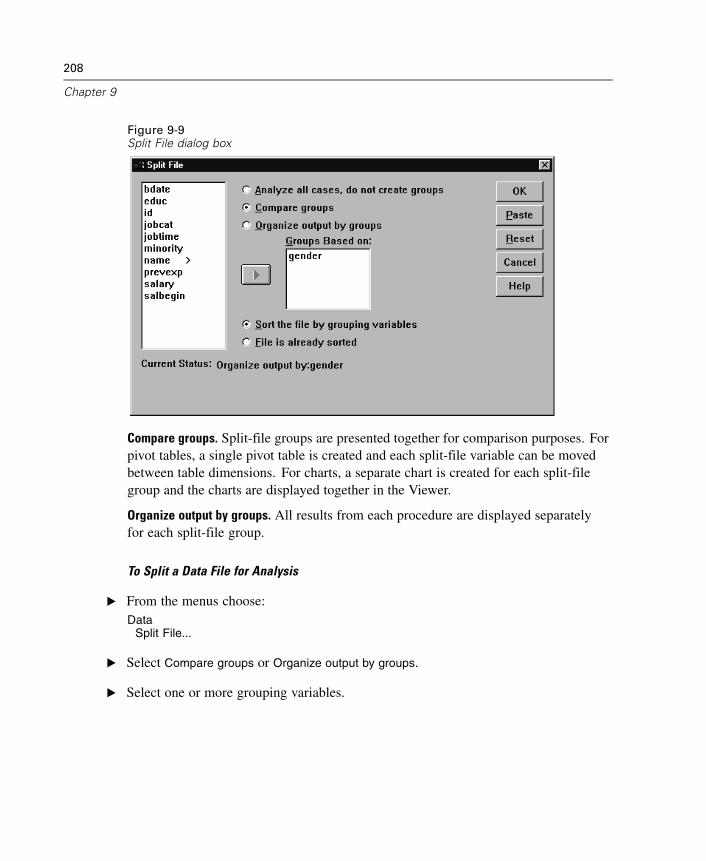
208

Chapter 9

Figure 9-9Split File dialog box

Compare groups. Split-file groups are presented together for comparison purposes. Forpivot tables, a single pivot table is created and each split-file variable can be movedbetween table dimensions. For charts, a separate chart is created for each split-filegroup and the charts are displayed together in the Viewer.

Organize output by groups. All results from each procedure are displayed separatelyfor each split-file group.

To Split a Data File for Analysis


Split File...

E Select Compare groups or Organize output by groups.

E Select one or more grouping variables.

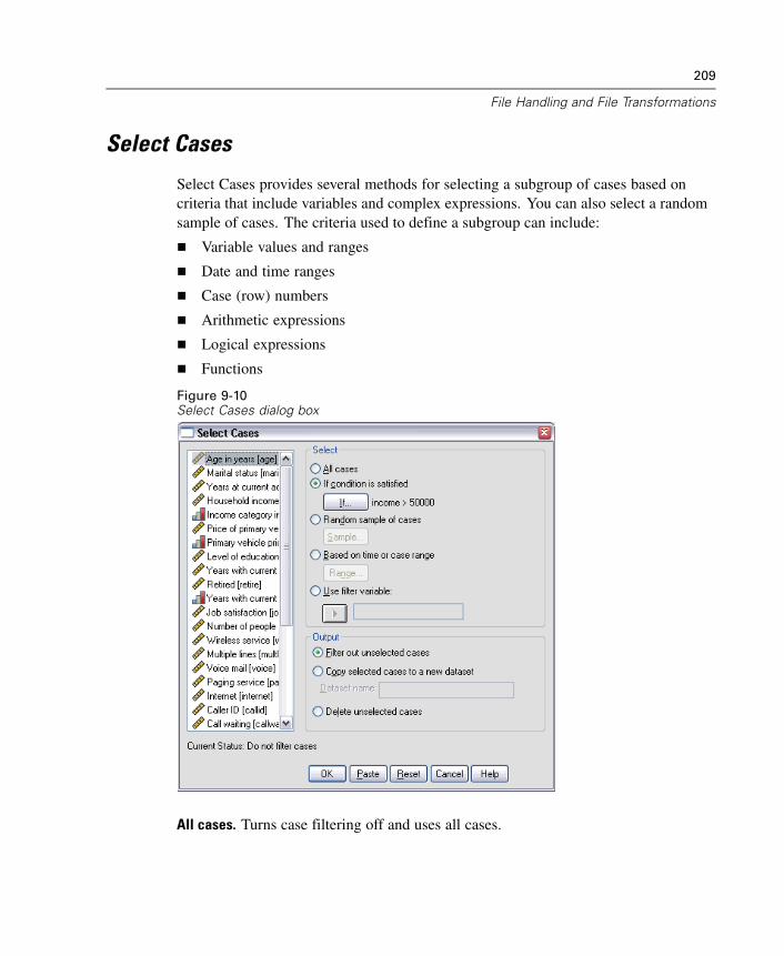
209


Select Cases

Select Cases provides several methods for selecting a subgroup of cases based oncriteria that include variables and complex expressions. You can also select a randomsample of cases. The criteria used to define a subgroup can include:

Variable values and ranges

Date and time ranges

Case (row) numbers

Arithmetic expressions

Logical expressions

Functions

Figure 9-10Select Cases dialog box

All cases. Turns case filtering off and uses all cases.

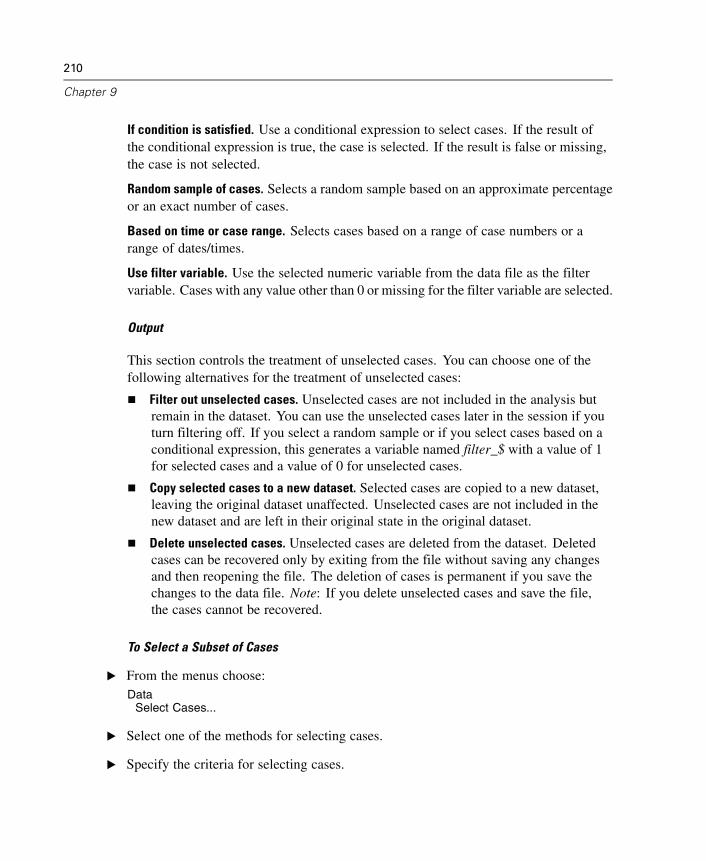
210

Chapter 9

If condition is satisfied. Use a conditional expression to select cases. If the result ofthe conditional expression is true, the case is selected. If the result is false or missing,the case is not selected.

Random sample of cases. Selects a random sample based on an approximate percentageor an exact number of cases.

Based on time or case range. Selects cases based on a range of case numbers or arange of dates/times.

Use filter variable. Use the selected numeric variable from the data file as the filtervariable. Cases with any value other than 0 or missing for the filter variable are selected.

Output

This section controls the treatment of unselected cases. You can choose one of thefollowing alternatives for the treatment of unselected cases:

Filter out unselected cases. Unselected cases are not included in the analysis butremain in the dataset. You can use the unselected cases later in the session if youturn filtering off. If you select a random sample or if you select cases based on aconditional expression, this generates a variable named filter_$ with a value of 1for selected cases and a value of 0 for unselected cases.

Copy selected cases to a new dataset. Selected cases are copied to a new dataset,leaving the original dataset unaffected. Unselected cases are not included in thenew dataset and are left in their original state in the original dataset.

Delete unselected cases. Unselected cases are deleted from the dataset. Deletedcases can be recovered only by exiting from the file without saving any changesand then reopening the file. The deletion of cases is permanent if you save thechanges to the data file. Note: If you delete unselected cases and save the file,the cases cannot be recovered.

To Select a Subset of Cases


Select Cases...

E Select one of the methods for selecting cases.

E Specify the criteria for selecting cases.

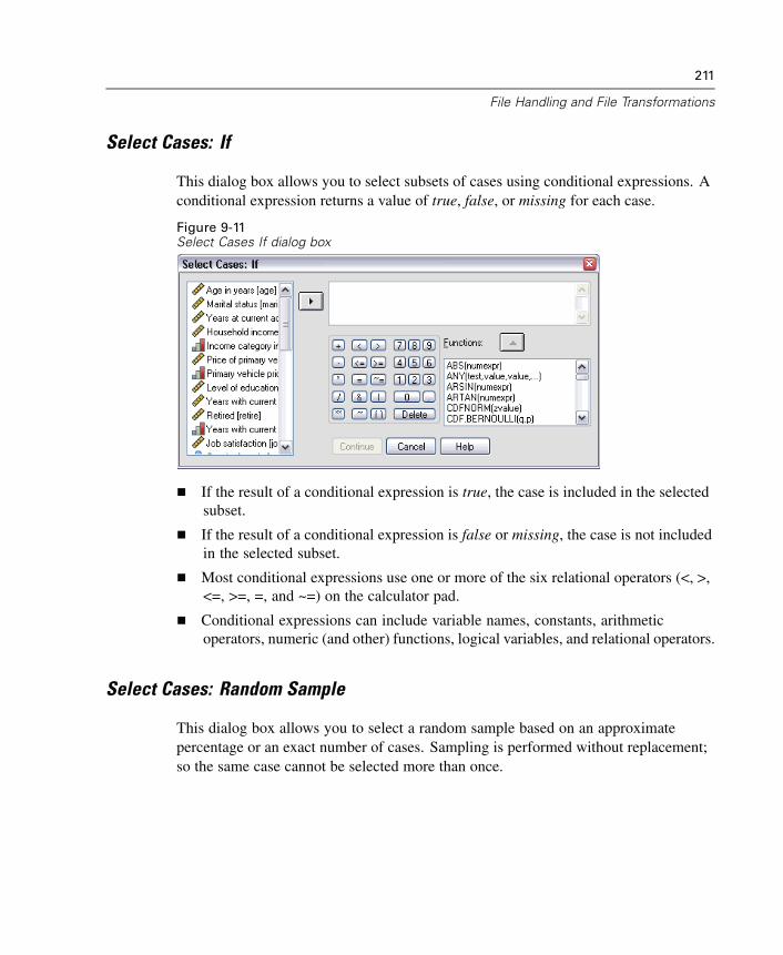
211


Select Cases: If

This dialog box allows you to select subsets of cases using conditional expressions. Aconditional expression returns a value of true, false, or missing for each case.

Figure 9-11Select Cases If dialog box

If the result of a conditional expression is true, the case is included in the selectedsubset.

If the result of a conditional expression is false or missing, the case is not includedin the selected subset.

Most conditional expressions use one or more of the six relational operators (<, >,<=, >=, =, and ~=) on the calculator pad.

Conditional expressions can include variable names, constants, arithmeticoperators, numeric (and other) functions, logical variables, and relational operators.

Select Cases: Random Sample

This dialog box allows you to select a random sample based on an approximatepercentage or an exact number of cases. Sampling is performed without replacement;so the same case cannot be selected more than once.

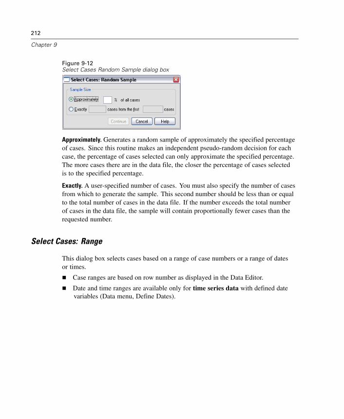
212

Chapter 9

Figure 9-12Select Cases Random Sample dialog box

Approximately. Generates a random sample of approximately the specified percentageof cases. Since this routine makes an independent pseudo-random decision for eachcase, the percentage of cases selected can only approximate the specified percentage.The more cases there are in the data file, the closer the percentage of cases selectedis to the specified percentage.

Exactly. A user-specified number of cases. You must also specify the number of casesfrom which to generate the sample. This second number should be less than or equalto the total number of cases in the data file. If the number exceeds the total numberof cases in the data file, the sample will contain proportionally fewer cases than therequested number.

Select Cases: Range

This dialog box selects cases based on a range of case numbers or a range of datesor times.

Case ranges are based on row number as displayed in the Data Editor.

Date and time ranges are available only for time series data with defined datevariables (Data menu, Define Dates).

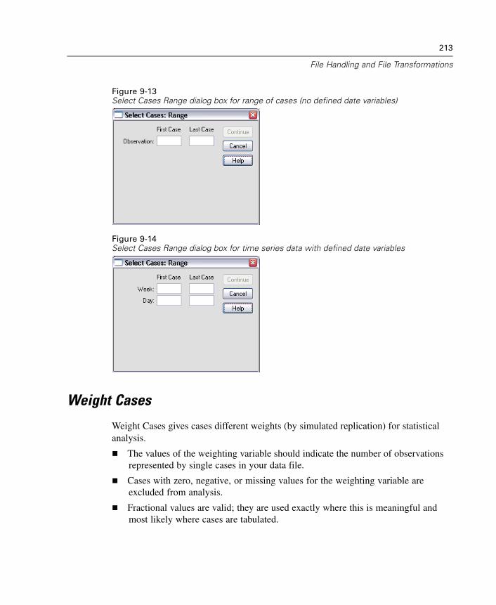
213


Figure 9-13Select Cases Range dialog box for range of cases (no defined date variables)

Figure 9-14Select Cases Range dialog box for time series data with defined date variables

Weight Cases

Weight Cases gives cases different weights (by simulated replication) for statisticalanalysis.

The values of the weighting variable should indicate the number of observationsrepresented by single cases in your data file.

Cases with zero, negative, or missing values for the weighting variable areexcluded from analysis.

Fractional values are valid; they are used exactly where this is meaningful andmost likely where cases are tabulated.

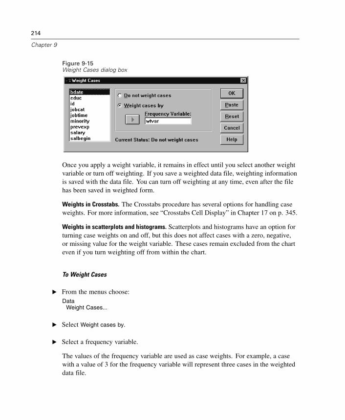
214

Chapter 9

Figure 9-15Weight Cases dialog box

Once you apply a weight variable, it remains in effect until you select another weightvariable or turn off weighting. If you save a weighted data file, weighting informationis saved with the data file. You can turn off weighting at any time, even after the filehas been saved in weighted form.

Weights in Crosstabs. The Crosstabs procedure has several options for handling caseweights. For more information, see “Crosstabs Cell Display” in Chapter 17 on p. 345.

Weights in scatterplots and histograms. Scatterplots and histograms have an option forturning case weights on and off, but this does not affect cases with a zero, negative,or missing value for the weight variable. These cases remain excluded from the charteven if you turn weighting off from within the chart.

To Weight Cases


Weight Cases...

E Select Weight cases by.

E Select a frequency variable.

The values of the frequency variable are used as case weights. For example, a casewith a value of 3 for the frequency variable will represent three cases in the weighteddata file.

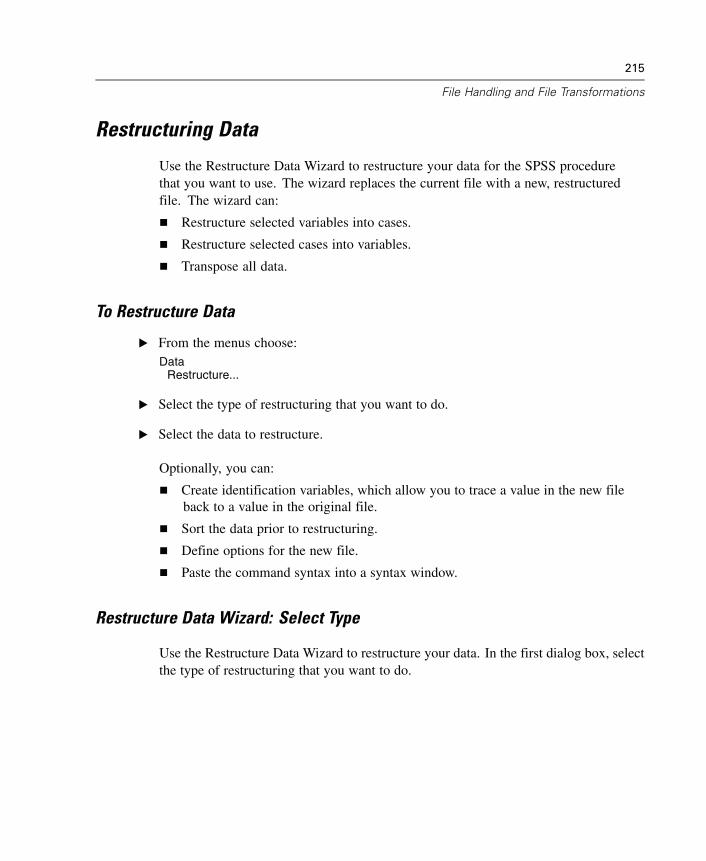
215


Restructuring Data

Use the Restructure Data Wizard to restructure your data for the SPSS procedurethat you want to use. The wizard replaces the current file with a new, restructuredfile. The wizard can:

Restructure selected variables into cases.

Restructure selected cases into variables.

Transpose all data.

To Restructure Data


Restructure...

E Select the type of restructuring that you want to do.

E Select the data to restructure.


Create identification variables, which allow you to trace a value in the new fileback to a value in the original file.

Sort the data prior to restructuring.

Define options for the new file.

Paste the command syntax into a syntax window.

Restructure Data Wizard: Select Type

Use the Restructure Data Wizard to restructure your data. In the first dialog box, selectthe type of restructuring that you want to do.

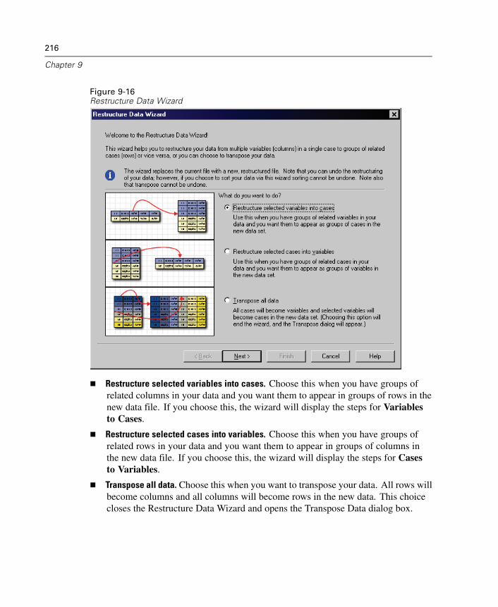
216

Chapter 9

Figure 9-16Restructure Data Wizard

Restructure selected variables into cases. Choose this when you have groups ofrelated columns in your data and you want them to appear in groups of rows in thenew data file. If you choose this, the wizard will display the steps for Variablesto Cases.

Restructure selected cases into variables. Choose this when you have groups ofrelated rows in your data and you want them to appear in groups of columns inthe new data file. If you choose this, the wizard will display the steps for Casesto Variables.

Transpose all data. Choose this when you want to transpose your data. All rows willbecome columns and all columns will become rows in the new data. This choicecloses the Restructure Data Wizard and opens the Transpose Data dialog box.

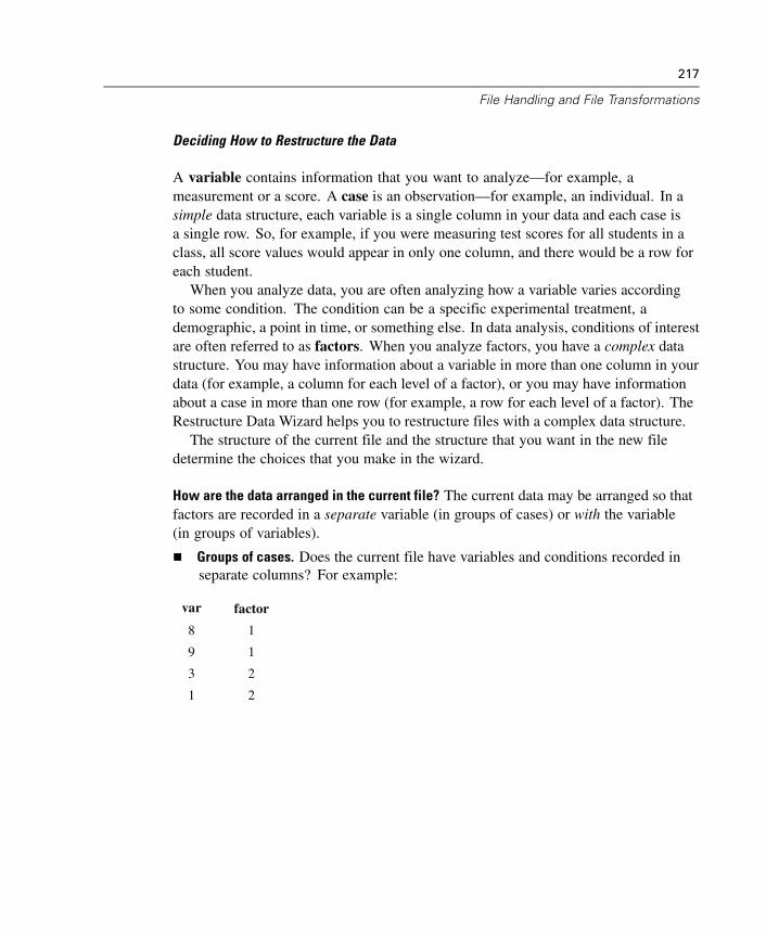
217


Deciding How to Restructure the Data

A variable contains information that you want to analyze—for example, ameasurement or a score. A case is an observation—for example, an individual. In asimple data structure, each variable is a single column in your data and each case isa single row. So, for example, if you were measuring test scores for all students in aclass, all score values would appear in only one column, and there would be a row foreach student.

When you analyze data, you are often analyzing how a variable varies accordingto some condition. The condition can be a specific experimental treatment, ademographic, a point in time, or something else. In data analysis, conditions of interestare often referred to as factors. When you analyze factors, you have a complex datastructure. You may have information about a variable in more than one column in yourdata (for example, a column for each level of a factor), or you may have informationabout a case in more than one row (for example, a row for each level of a factor). TheRestructure Data Wizard helps you to restructure files with a complex data structure.

The structure of the current file and the structure that you want in the new filedetermine the choices that you make in the wizard.

How are the data arranged in the current file? The current data may be arranged so thatfactors are recorded in a separate variable (in groups of cases) or with the variable(in groups of variables).

Groups of cases. Does the current file have variables and conditions recorded inseparate columns? For example:

var factor

8 1

9 1

3 2

1 2

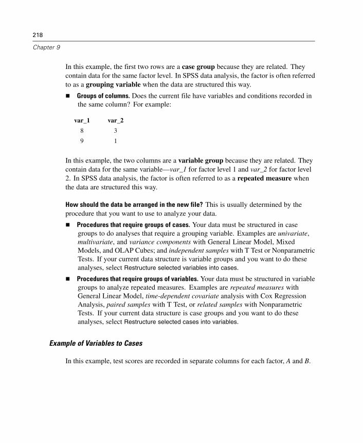
218

Chapter 9

In this example, the first two rows are a case group because they are related. Theycontain data for the same factor level. In SPSS data analysis, the factor is often referredto as a grouping variable when the data are structured this way.

Groups of columns. Does the current file have variables and conditions recorded inthe same column? For example:

var_1 var_2

8 3

9 1

In this example, the two columns are a variable group because they are related. Theycontain data for the same variable—var_1 for factor level 1 and var_2 for factor level2. In SPSS data analysis, the factor is often referred to as a repeated measure whenthe data are structured this way.

How should the data be arranged in the new file? This is usually determined by theprocedure that you want to use to analyze your data.

Procedures that require groups of cases. Your data must be structured in casegroups to do analyses that require a grouping variable. Examples are univariate,multivariate, and variance components with General Linear Model, MixedModels, and OLAP Cubes; and independent samples with T Test or NonparametricTests. If your current data structure is variable groups and you want to do theseanalyses, select Restructure selected variables into cases.

Procedures that require groups of variables. Your data must be structured in variablegroups to analyze repeated measures. Examples are repeated measures withGeneral Linear Model, time-dependent covariate analysis with Cox RegressionAnalysis, paired samples with T Test, or related samples with NonparametricTests. If your current data structure is case groups and you want to do theseanalyses, select Restructure selected cases into variables.

Example of Variables to Cases

In this example, test scores are recorded in separate columns for each factor, A and B.

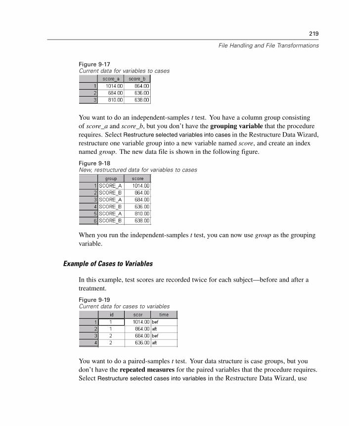
219


Figure 9-17Current data for variables to cases

You want to do an independent-samples t test. You have a column group consistingof score_a and score_b, but you don’t have the grouping variable that the procedurerequires. Select Restructure selected variables into cases in the Restructure Data Wizard,restructure one variable group into a new variable named score, and create an indexnamed group. The new data file is shown in the following figure.

Figure 9-18New, restructured data for variables to cases

When you run the independent-samples t test, you can now use group as the groupingvariable.

Example of Cases to Variables

In this example, test scores are recorded twice for each subject—before and after atreatment.

Figure 9-19Current data for cases to variables

You want to do a paired-samples t test. Your data structure is case groups, but youdon’t have the repeated measures for the paired variables that the procedure requires.Select Restructure selected cases into variables in the Restructure Data Wizard, use

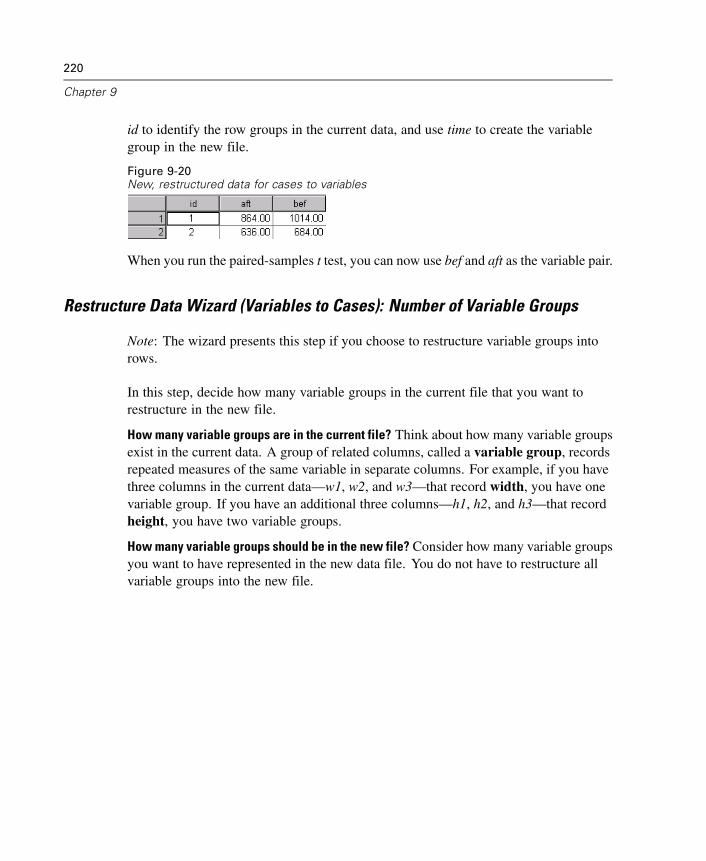
220

Chapter 9

id to identify the row groups in the current data, and use time to create the variablegroup in the new file.

Figure 9-20New, restructured data for cases to variables

When you run the paired-samples t test, you can now use bef and aft as the variable pair.

Restructure Data Wizard (Variables to Cases): Number of Variable Groups

Note: The wizard presents this step if you choose to restructure variable groups intorows.

In this step, decide how many variable groups in the current file that you want torestructure in the new file.

How many variable groups are in the current file? Think about how many variable groupsexist in the current data. A group of related columns, called a variable group, recordsrepeated measures of the same variable in separate columns. For example, if you havethree columns in the current data—w1, w2, and w3—that record width, you have onevariable group. If you have an additional three columns—h1, h2, and h3—that recordheight, you have two variable groups.

How many variable groups should be in the new file? Consider how many variable groupsyou want to have represented in the new data file. You do not have to restructure allvariable groups into the new file.

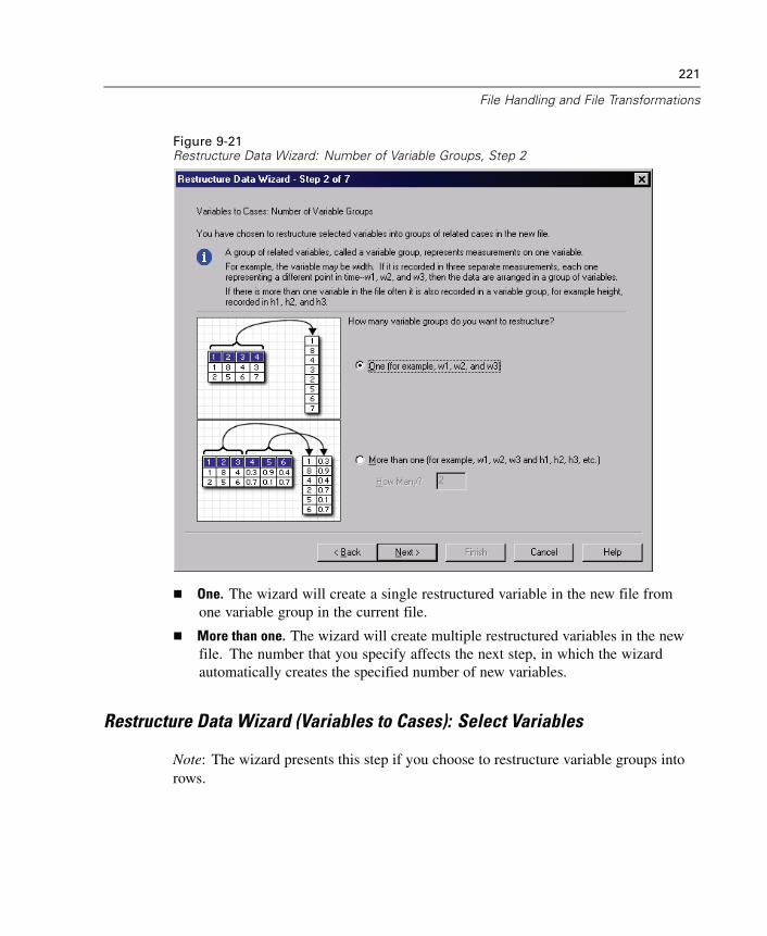
221


Figure 9-21Restructure Data Wizard: Number of Variable Groups, Step 2

One. The wizard will create a single restructured variable in the new file fromone variable group in the current file.

More than one. The wizard will create multiple restructured variables in the newfile. The number that you specify affects the next step, in which the wizardautomatically creates the specified number of new variables.

Restructure Data Wizard (Variables to Cases): Select Variables


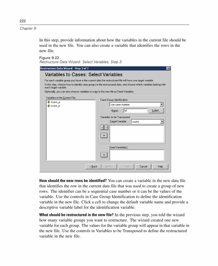
222

Chapter 9

In this step, provide information about how the variables in the current file should beused in the new file. You can also create a variable that identifies the rows in thenew file.

Figure 9-22Restructure Data Wizard: Select Variables, Step 3

How should the new rows be identified? You can create a variable in the new data filethat identifies the row in the current data file that was used to create a group of newrows. The identifier can be a sequential case number or it can be the values of thevariable. Use the controls in Case Group Identification to define the identificationvariable in the new file. Click a cell to change the default variable name and provide adescriptive variable label for the identification variable.

What should be restructured in the new file? In the previous step, you told the wizardhow many variable groups you want to restructure. The wizard created one newvariable for each group. The values for the variable group will appear in that variable inthe new file. Use the controls in Variables to be Transposed to define the restructuredvariable in the new file.

223


To Specify One Restructured Variable

E Put the variables that make up the variable group that you want to transform into theVariables to be Transposed list. All of the variables in the group must be of the sametype (numeric or string).

You can include the same variable more than once in the variable group (variables arecopied rather than moved from the source variable list); its values are repeated inthe new file.

To Specify Multiple Restructured Variables

E Select the first target variable that you want to define from the Target Variabledrop-down list.

E Put the variables that make up the variable group that you want to transform into theVariables to be Transposed list. All of the variables in the group must be of the sametype (numeric or string). You can include the same variable more than once in thevariable group. (A variable is copied rather than moved from the source variable list,and its values are repeated in the new file.)

E Select the next target variable that you want to define, and repeat the variable selectionprocess for all available target variables.

Although you can include the same variable more than once in the same targetvariable group, you cannot include the same variable in more than one targetvariable group.

Each target variable group list must contain the same number of variables.(Variables that are listed more than once are included in the count.)

The number of target variable groups is determined by the number of variablegroups that you specified in the previous step. You can change the default variablenames here, but you must return to the previous step to change the number ofvariable groups to restructure.

You must define variable groups (by selecting variables in the source list) for allavailable target variables before you can proceed to the next step.

What should be copied into the new file? Variables that aren’t restructured can be copiedinto the new file. Their values will be propagated in the new rows. Move variables thatyou want to copy into the new file into the Fixed Variable(s) list.

224

Chapter 9

Restructure Data Wizard (Variables to Cases): Create Index Variables


In this step, decide whether to create index variables. An index is a new variablethat sequentially identifies a row group based on the original variable from whichthe new row was created.

Figure 9-23Restructure Data Wizard: Create Index Variables, Step 4

How many index variables should be in the new file? Index variables can be used asgrouping variables in SPSS procedures. In most cases, a single index variable issufficient; however, if the variable groups in your current file reflect multiple factorlevels, multiple indices may be appropriate.

One. The wizard will create a single index variable.

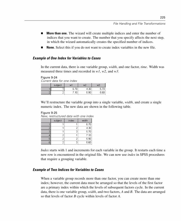
225


More than one. The wizard will create multiple indices and enter the number ofindices that you want to create. The number that you specify affects the next step,in which the wizard automatically creates the specified number of indices.

None. Select this if you do not want to create index variables in the new file.

Example of One Index for Variables to Cases

In the current data, there is one variable group, width, and one factor, time. Width wasmeasured three times and recorded in w1, w2, and w3.

Figure 9-24Current data for one index

We’ll restructure the variable group into a single variable, width, and create a singlenumeric index. The new data are shown in the following table.

Figure 9-25New, restructured data with one index

Index starts with 1 and increments for each variable in the group. It restarts each time anew row is encountered in the original file. We can now use index in SPSS proceduresthat require a grouping variable.

Example of Two Indices for Variables to Cases

When a variable group records more than one factor, you can create more than oneindex; however, the current data must be arranged so that the levels of the first factorare a primary index within which the levels of subsequent factors cycle. In the currentdata, there is one variable group, width, and two factors, A and B. The data are arrangedso that levels of factor B cycle within levels of factor A.

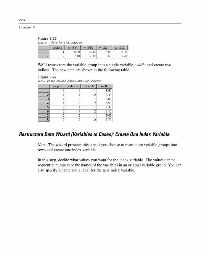
226

Chapter 9

Figure 9-26Current data for two indices

We’ll restructure the variable group into a single variable, width, and create twoindices. The new data are shown in the following table.

Figure 9-27New, restructured data with two indices

Restructure Data Wizard (Variables to Cases): Create One Index Variable

Note: The wizard presents this step if you choose to restructure variable groups intorows and create one index variable.

In this step, decide what values you want for the index variable. The values can besequential numbers or the names of the variables in an original variable group. You canalso specify a name and a label for the new index variable.

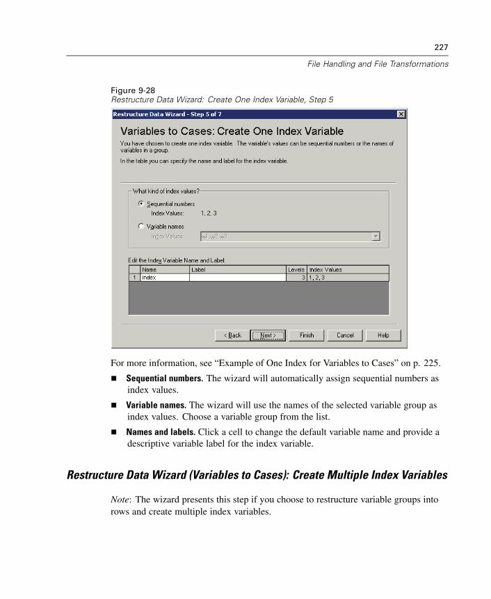
227


Figure 9-28Restructure Data Wizard: Create One Index Variable, Step 5

For more information, see “Example of One Index for Variables to Cases” on p. 225.

Sequential numbers. The wizard will automatically assign sequential numbers asindex values.

Variable names. The wizard will use the names of the selected variable group asindex values. Choose a variable group from the list.

Names and labels. Click a cell to change the default variable name and provide adescriptive variable label for the index variable.

Restructure Data Wizard (Variables to Cases): Create Multiple Index Variables

Note: The wizard presents this step if you choose to restructure variable groups intorows and create multiple index variables.

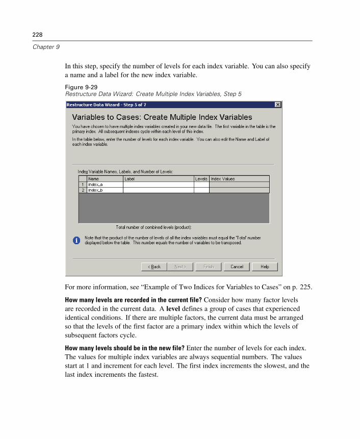
228

Chapter 9

In this step, specify the number of levels for each index variable. You can also specifya name and a label for the new index variable.

Figure 9-29Restructure Data Wizard: Create Multiple Index Variables, Step 5

For more information, see “Example of Two Indices for Variables to Cases” on p. 225.

How many levels are recorded in the current file? Consider how many factor levelsare recorded in the current data. A level defines a group of cases that experiencedidentical conditions. If there are multiple factors, the current data must be arrangedso that the levels of the first factor are a primary index within which the levels ofsubsequent factors cycle.

How many levels should be in the new file? Enter the number of levels for each index.The values for multiple index variables are always sequential numbers. The valuesstart at 1 and increment for each level. The first index increments the slowest, and thelast index increments the fastest.

229


Total combined levels. You cannot create more levels than exist in the current data.Because the restructured data will contain one row for each combination of treatments,the wizard checks the number of levels that you create. It will compare the productof the levels that you create to the number of variables in your variable groups. Theymust match.

Names and labels. Click a cell to change the default variable name and provide adescriptive variable label for the index variables.

Restructure Data Wizard (Variables to Cases): Options


In this step, specify options for the new, restructured file.

230

Chapter 9

Figure 9-30Restructure Data Wizard: Options, Step 6

Drop unselected variables? In the Select Variables step (step 3), you selected variablegroups to be restructured, variables to be copied, and an identification variable fromthe current data. The data from the selected variables will appear in the new file. Ifthere are other variables in the current data, you can choose to discard or keep them.

Keep missing data? The wizard checks each potential new row for null values. A nullvalue is a system-missing or blank value. You can choose to keep or discard rows thatcontain only null values.

Create a count variable? The wizard can create a count variable in the new file. Itcontains the number of new rows generated by a row in the current data. A countvariable may be useful if you choose to discard null values from the new file becausethat makes it possible to generate a different number of new rows for a given row in the

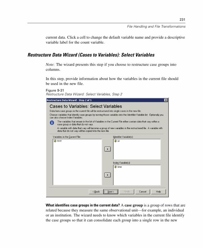
231


current data. Click a cell to change the default variable name and provide a descriptivevariable label for the count variable.

Restructure Data Wizard (Cases to Variables): Select Variables

Note: The wizard presents this step if you choose to restructure case groups intocolumns.

In this step, provide information about how the variables in the current file shouldbe used in the new file.

Figure 9-31Restructure Data Wizard: Select Variables, Step 2

What identifies case groups in the current data? A case group is a group of rows that arerelated because they measure the same observational unit—for example, an individualor an institution. The wizard needs to know which variables in the current file identifythe case groups so that it can consolidate each group into a single row in the new

232

Chapter 9

file. Move variables that identify case groups in the current file into the IdentifierVariable(s) list. Variables that are used to split the current data file are automaticallyused to identify case groups. Each time a new combination of identification valuesis encountered, the wizard will create a new row, so cases in the current file shouldbe sorted by values of the identification variables, in the same order that variables arelisted in the Identifier Variable(s) list. If the current data file isn’t already sorted,you can sort it in the next step.

How should the new variable groups be created in the new file? In the original data, avariable appears in a single column. In the new data file, that variable will appearin multiple new columns. Index variables are variables in the current data that thewizard should use to create the new columns. The restructured data will contain onenew variable for each unique value in these columns. Move the variables that shouldbe used to form the new variable groups to the Index Variable(s) list. When the wizardpresents options, you can also choose to order the new columns by index.

What happens to the other columns? The wizard automatically decides what to do withthe variables that remain in the Current File list. It checks each variable to see if thedata values vary within a case group. If they do, the wizard restructures the valuesinto a variable group in the new file. If they don’t, the wizard copies the values intothe new file.

Restructure Data Wizard (Cases to Variables): Sort Data


In this step, decide whether to sort the current file before restructuring it. Each time thewizard encounters a new combination of identification values, a new row is created, soit is important that the data are sorted by the variables that identify case groups.

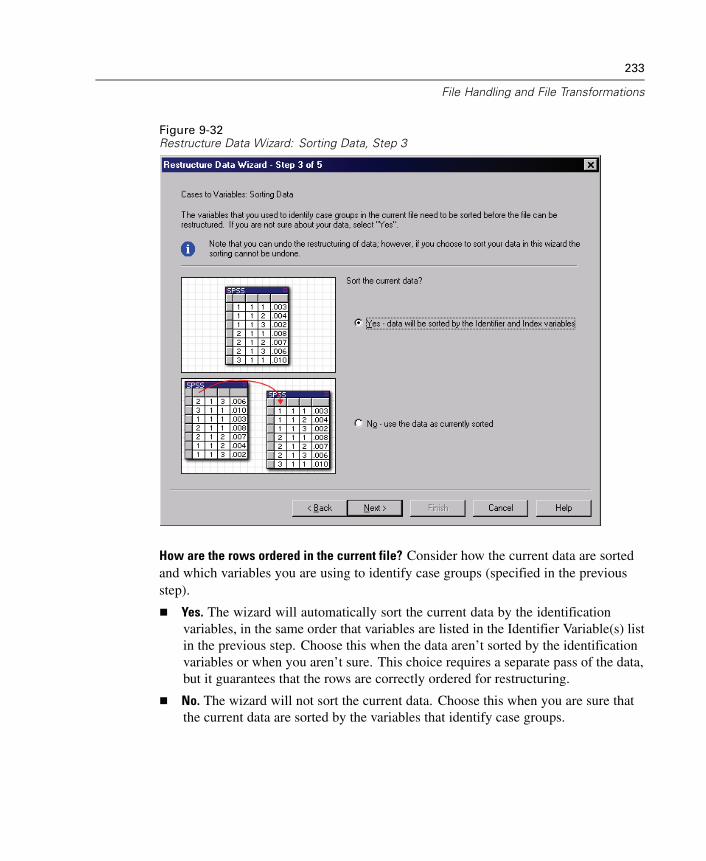
233


Figure 9-32Restructure Data Wizard: Sorting Data, Step 3

How are the rows ordered in the current file? Consider how the current data are sortedand which variables you are using to identify case groups (specified in the previousstep).

Yes. The wizard will automatically sort the current data by the identificationvariables, in the same order that variables are listed in the Identifier Variable(s) listin the previous step. Choose this when the data aren’t sorted by the identificationvariables or when you aren’t sure. This choice requires a separate pass of the data,but it guarantees that the rows are correctly ordered for restructuring.

No. The wizard will not sort the current data. Choose this when you are sure thatthe current data are sorted by the variables that identify case groups.

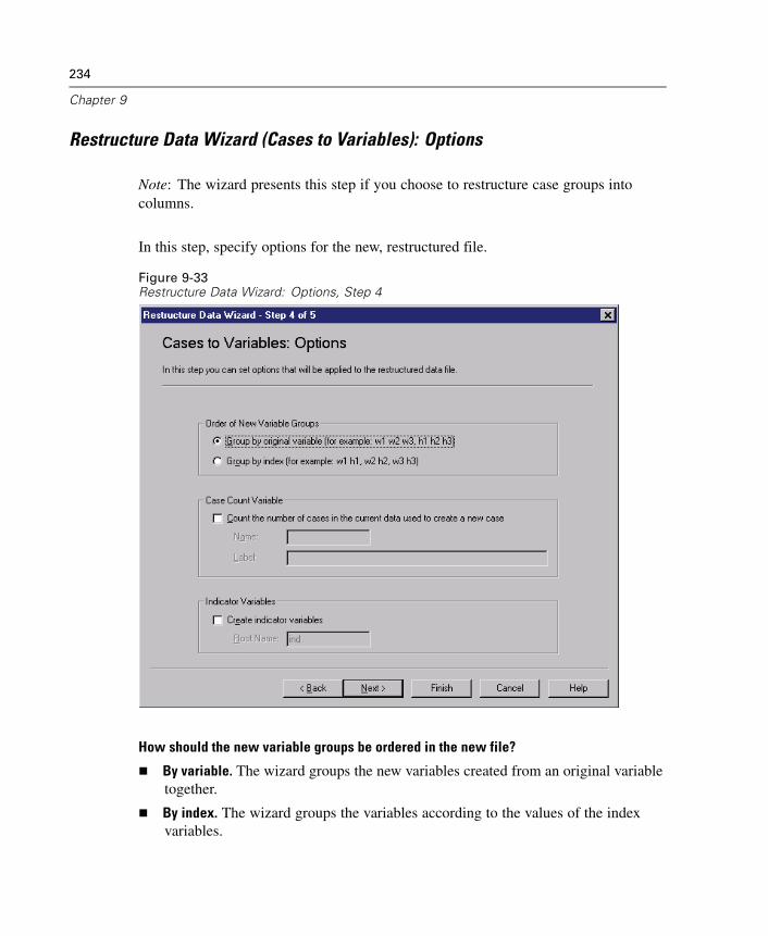
234

Chapter 9

Restructure Data Wizard (Cases to Variables): Options


In this step, specify options for the new, restructured file.

Figure 9-33Restructure Data Wizard: Options, Step 4

How should the new variable groups be ordered in the new file?

By variable. The wizard groups the new variables created from an original variabletogether.

By index. The wizard groups the variables according to the values of the indexvariables.

235


Example. The variables to be restructured are w and h, and the index is month:

w h month

Grouping by variable results in:

w.jan w.feb h.jan

Grouping by index results in:

w.jan h.jan w.feb

Create a count variable? The wizard can create a count variable in the new file. Itcontains the number of rows in the current data that were used to create a row in thenew data file.

Create indicator variables? The wizard can use the index variables to create indicatorvariables in the new data file. It creates one new variable for each unique value of theindex variable. The indicator variables signal the presence or absence of a value for acase. An indicator variable has the value of 1 if the case has a value; otherwise, it is 0.

Example. The index variable is product. It records the products that a customerpurchased. The original data are:

customer product

1 chick

1 eggs

2 eggs

3 chick

Creating an indicator variable results in one new variable for each unique value ofproduct. The restructured data are:

customer indchick indeggs

1 1 1

2 0 1

3 1 0

236

Chapter 9

In this example, the restructured data could be used to get frequency counts of theproducts that customers buy.

Restructure Data Wizard: Finish

This is the final step of the Restructure Data Wizard. Decide what to do with yourspecifications.

Figure 9-34Restructure Data Wizard: Finish

237


Restructure now. The wizard will create the new, restructured file. Choose thisif you want to replace the current file immediately. Note: If original data areweighted, the new data will be weighted unless the variable that is used as theweight is restructured or dropped from the new file.

Paste syntax. The wizard will paste the syntax it generates into a syntax window.Choose this when you are not ready to replace the current file, when you want tomodify the syntax, or when you want to save it for future use.

Chapter

10Working with Output

When you run a procedure, the results are displayed in a window called the Viewer.In this window, you can easily navigate to the output that you want to see. You canalso manipulate the output and create a document that contains precisely the outputthat you want.

Viewer

Results are displayed in the Viewer. You can use the Viewer to:

Browse results.

Show or hide selected tables and charts.

Change the display order of results by moving selected items.

Move items between the Viewer and other applications.

239

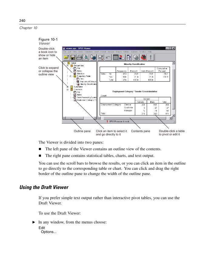
240

Chapter 10

Figure 10-1Viewer

The Viewer is divided into two panes:

The left pane of the Viewer contains an outline view of the contents.

The right pane contains statistical tables, charts, and text output.

You can use the scroll bars to browse the results, or you can click an item in the outlineto go directly to the corresponding table or chart. You can click and drag the rightborder of the outline pane to change the width of the outline pane.

Using the Draft Viewer

If you prefer simple text output rather than interactive pivot tables, you can use theDraft Viewer.

To use the Draft Viewer:

E In any window, from the menus choose:Edit

Options...

241

Working with Output

E On the General tab, click Draft for the output viewer type.

E To change the format options for Draft Viewer output, click the Draft Viewer tab.

For more information, see “Draft Viewer” in Chapter 11 on p. 271. You can alsosearch the Help facility to learn more:

E In any window, from the menus choose:Help

Topics

E Click the Index tab in the Help Topics window.

E Type draft viewer, and then double-click the index entry.

Showing and Hiding Results

In the Viewer, you can selectively show and hide individual tables or results froman entire procedure. This process is useful when you want to shorten the amount ofvisible output in the contents pane.

To Hide Tables and Charts

E Double-click the item’s book icon in the outline pane of the Viewer.

or

E Click the item to select it.


Hide

or

E Click the closed book (Hide) icon on the Outlining toolbar.

The open book (Show) icon becomes the active icon, indicating that the item is nowhidden.

To Hide Procedure Results

E Click the box to the left of the procedure name in the outline pane.

242

Chapter 10

This hides all results from the procedure and collapses the outline view.

Moving, Deleting, and Copying Output

You can rearrange the results by copying, moving, or deleting an item or a groupof items.

To Move Output in the Viewer

E Click an item in the outline or contents pane. (Shift-click to select multiple items, orCtrl-click to select noncontiguous items.)

E Click and drag selected items (hold down the mouse button while dragging).

E Release the mouse button on the item just above the location where you want to dropthe moved items.

You can also move items by using Cut and Paste After on the Edit menu.

To Delete Output in the Viewer


E Press Delete.

or


Delete

To Copy Output in the Viewer


E Hold down the Ctrl key while you click and drag selected items (hold down the mousebutton while dragging).

E Release the mouse button to drop the items where you want them.

243

Working with Output

You can also copy items by using Copy and Paste After on the Edit menu.

Changing Initial Alignment

By default, all results are initially left-aligned. You can change the initial alignment(choose Options on the Edit menu, then click the Viewer tab) at any time.

Changing Alignment of Output Items

E In the outline or contents pane, click the items that you want to align (Shift-click orCtrl-click to select multiple items).

E From the menus choose:Format

Align Left

Other alignment options include Center and Align Right.

Note: All results are displayed left-aligned in the Viewer. Only the alignment ofprinted results is affected by the alignment settings. Centered and right-aligned itemsare identified by a small symbol above and to the left of the item.

Viewer Outline

The outline pane provides a table of contents of the Viewer document. You can use theoutline pane to navigate through your results and control the display. Most actions inthe outline pane have a corresponding effect on the contents pane.

Selecting an item in the outline pane displays the corresponding item in thecontents pane.

Moving an item in the outline pane moves the corresponding item in the contentspane.

Collapsing the outline view hides the results from all items in the collapsed levels.

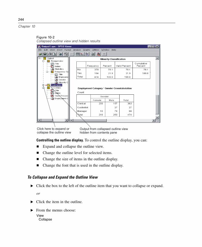
244

Chapter 10

Figure 10-2Collapsed outline view and hidden results

Click here to expand or collapse the outline view

Output from collapsed outline viewhidden from contents pane

Viewer

Controlling the outline display. To control the outline display, you can:

Expand and collapse the outline view.

Change the outline level for selected items.

Change the size of items in the outline display.

Change the font that is used in the outline display.

To Collapse and Expand the Outline View

E Click the box to the left of the outline item that you want to collapse or expand.

or

E Click the item in the outline.


Collapse

245

Working with Output

orView

Expand

To Change the Outline Level

E Click the item in the outline pane.

E Click the left arrow on the Outlining toolbar to promote the item (move the item tothe left).

E Click the right arrow on the Outlining toolbar to demote the item (move the itemto the right).

or

From the menus choose:Edit

OutlinePromote

orEdit

OutlineDemote

Changing the outline level is particularly useful after you move items in the outlinelevel. Moving items can change the outline level of the items, and you can use the left-and right-arrow buttons on the Outlining toolbar to restore the original outline level.

To Change the Size of Outline Items


Outline SizeSmall

Other options include Medium and Large.

The icons and their associated text change size.

246

Chapter 10

To Change the Font in the Outline


Outline Font...

E Select a font.

Adding Items to the Viewer

In the Viewer, you can add items such as titles, new text, charts, or material fromother applications.

To Add a Title or Text

Text items that are not connected to a table or chart can be added to the Viewer.

E Click the table, chart, or other object that will precede the title or text.

E From the menus choose:Insert

New Title

orInsert

New Text

E Double-click the new object.

E Enter the text that you want at this location.

To Add a Text File

E In the outline pane or contents pane of the Viewer, click the table, chart, or other objectthat will precede the text.

E From the menus choose:Insert

Text File...

E Select a text file.

247

Working with Output

To edit the text, double-click it.

Using Output in Other Applications

Pivot tables and charts can be copied and pasted into another Windows application,such as a word-processing program or a spreadsheet. You can paste the pivot tables orcharts in various formats, including the following formats:

Embedded object. For applications that support ActiveX objects, you can embed pivottables and interactive charts. After you paste the table, it can be activated in place bydouble-clicking it, and then it can be edited as if in the Viewer.

Picture (metafile). You can paste pivot tables, text output, and charts as metafilepictures. The picture format can be resized in the other application, and sometimes alimited amount of editing can be done with the facilities of the other application. Pivottables that are pasted as pictures retain all borders and font characteristics.

RTF (rich text format). Pivot tables can be pasted into other applications in RTF format.In most applications, this means that the pivot table is pasted as a table that can then beedited in the other application.

Bitmap. Charts can be pasted into other applications as bitmaps.

BIFF. The contents of a table can be pasted into a spreadsheet and retain numericprecision.

Text. The contents of a table can be copied and pasted as text. This process can be usefulfor applications such as e-mail, where the application can accept or transmit only text.

To Copy a Table or Chart

E Select the table or chart to be copied.


Copy

To Copy and Paste Results into Another Application

E Copy the results in the Viewer.

248

Chapter 10

E From the menus in the target application choose:Edit

Paste

orEdit

Paste Special...

Paste. Output is copied to the clipboard in a number of formats. Each applicationdetermines the “best” format to use for Paste. In many applications, Paste will pasteresults as a picture (metafile). For word-processing applications, Paste will pastepivot tables in RTF format, which pastes the pivot table as a table. For spreadsheetapplications, Paste will paste pivot tables in BIFF format. Charts are pasted asmetafiles.

Paste Special. Results are copied to the clipboard in multiple formats. Paste Specialallows you to select the format that you want from the list of formats that are availableto the target application.

To Embed a Table in Another Application

You can embed pivot tables and interactive charts in other applications in ActiveXformat. An embedded object can be activated in place by double-clicking it, and theobject can then be edited and pivoted as if in the Viewer.

If you have applications that support ActiveX objects:

E Double-click the file objs-on.bat, which is located in the directory in which SPSS isinstalled.

This action turns on ActiveX embedding for pivot tables. The file objs-off.bat turnsActiveX embedding off.

To embed a pivot table or interactive chart in another application:

E In the Viewer, copy the table.


Paste Special...

E From the list, select SPSS Pivot Table Object or SPSS Graphics Control Object.

249

Working with Output

The target application must support ActiveX objects. See the application’sdocumentation for information about ActiveX support. Some applications that donot support ActiveX may initially accept ActiveX pivot tables but may then exhibitunstable behavior. Do not rely on embedded objects until you have tested theapplication’s stability with embedded ActiveX objects.

To Paste a Pivot Table or Chart as a Picture (Metafile)

E In the Viewer, copy the table or chart.


Paste Special...

E From the list, select Picture.

The item is pasted as a metafile. Only the layer and columns that were visible whenthe item was copied are available in the metafile. Other layers or hidden columnsare not available.

To Paste a Pivot Table as a Table (RTF)

E In the Viewer, copy the pivot table.


Paste Special...

E From the list, select Formatted Text (RTF) or Rich Text Format.

The pivot table is pasted as a table. Only the layer and columns that were visible whenthe item was copied are pasted into the table. Other layers or hidden columns are notavailable. You can copy and paste only one pivot table at a time in this format.

To Paste a Pivot Table as Text

E In the Viewer, copy the table.


Paste Special...

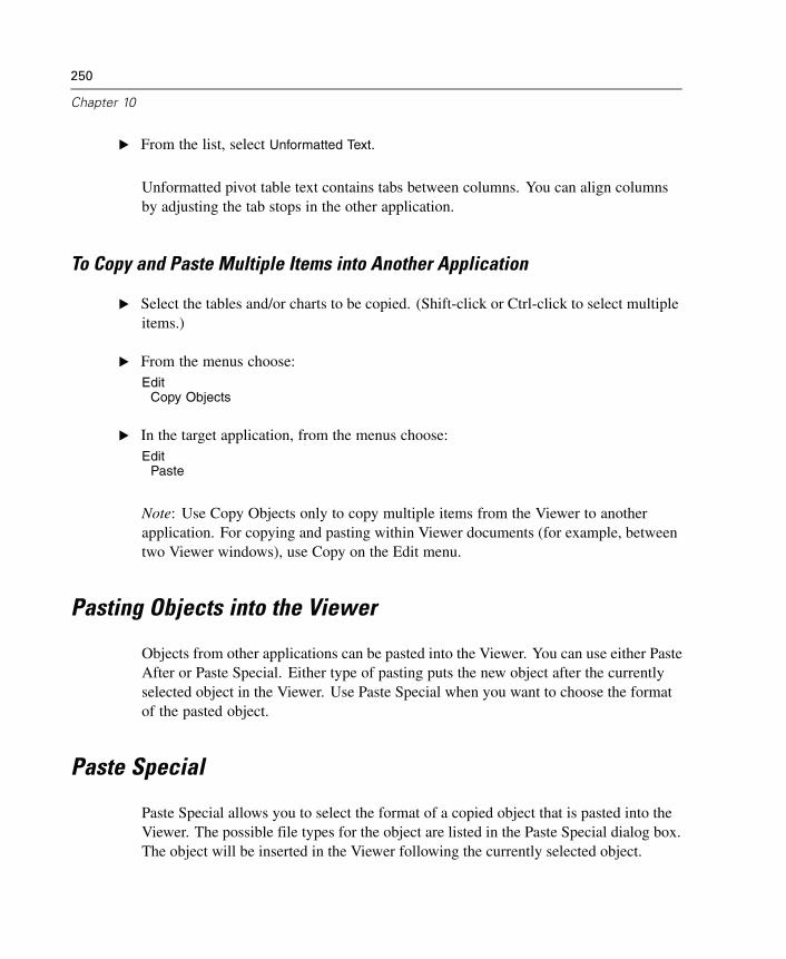
250

Chapter 10

E From the list, select Unformatted Text.

Unformatted pivot table text contains tabs between columns. You can align columnsby adjusting the tab stops in the other application.

To Copy and Paste Multiple Items into Another Application

E Select the tables and/or charts to be copied. (Shift-click or Ctrl-click to select multipleitems.)


Copy Objects

E In the target application, from the menus choose:Edit

Paste

Note: Use Copy Objects only to copy multiple items from the Viewer to anotherapplication. For copying and pasting within Viewer documents (for example, betweentwo Viewer windows), use Copy on the Edit menu.

Pasting Objects into the Viewer

Objects from other applications can be pasted into the Viewer. You can use either PasteAfter or Paste Special. Either type of pasting puts the new object after the currentlyselected object in the Viewer. Use Paste Special when you want to choose the formatof the pasted object.

Paste Special

Paste Special allows you to select the format of a copied object that is pasted into theViewer. The possible file types for the object are listed in the Paste Special dialog box.The object will be inserted in the Viewer following the currently selected object.

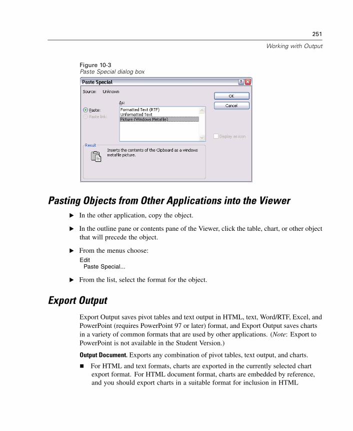
251

Working with Output

Figure 10-3Paste Special dialog box

Pasting Objects from Other Applications into the ViewerE In the other application, copy the object.

E In the outline pane or contents pane of the Viewer, click the table, chart, or other objectthat will precede the object.


Paste Special...

E From the list, select the format for the object.

Export OutputExport Output saves pivot tables and text output in HTML, text, Word/RTF, Excel, andPowerPoint (requires PowerPoint 97 or later) format, and Export Output saves chartsin a variety of common formats that are used by other applications. (Note: Export toPowerPoint is not available in the Student Version.)

Output Document. Exports any combination of pivot tables, text output, and charts.

For HTML and text formats, charts are exported in the currently selected chartexport format. For HTML document format, charts are embedded by reference,and you should export charts in a suitable format for inclusion in HTML

252

Chapter 10

documents. For text document format, a line is inserted in the text file for eachchart, indicating the filename of the exported chart.

For Word/RTF format, charts are exported in Windows metafile format andembedded in the Word document.

Charts are not included in Excel documents.

For PowerPoint format, charts are exported in TIFF format and embedded in thePowerPoint file.

Output Document (No Charts). Exports pivot tables and text output. Any charts in theViewer are ignored.

Charts Only. Available export formats include: Windows metafile (WMF), enhancedmetafile (EMF), Windows bitmap (BMP), encapsulated PostScript (EPS), JPEG, TIFF,PNG, and Macintosh PICT.

Export What. You can export all objects in the Viewer, all visible objects, or onlyselected objects.

Export Format. For output documents, the available options are HTML, text, Excel,Word/RTF, and PowerPoint; for HTML and text format, charts are exported in thecurrently selected chart format in the Options dialog box for the selected format.For Charts Only, choose a chart export format from the drop-down list. For outputdocuments, pivot tables and text are exported in the following manner:

HTML file (*.htm). Pivot tables are exported as HTML tables. Text output is exportedas preformatted HTML.

Text file (*.txt). Pivot tables can be exported in tab-separated or space-separatedformat. All text output is exported in space-separated format.

Excel file (*.xls). Pivot table rows, columns, and cells are exported as Excel rows,columns, and cells, with all formatting attributes intact—for example, cell borders,font styles, and background colors. Text output is exported with all font attributesintact. Each line in the text output is a row in the Excel file, with the entire contentsof the line contained in a single cell.

Word/RTF file (*.doc). Pivot tables are exported as Word tables with all formattingattributes intact—for example, cell borders, font styles, background colors, andso on. Text output is exported as formatted RTF. Text output in SPSS is alwaysdisplayed in a fixed-pitch (monospaced) font and is exported with the same font

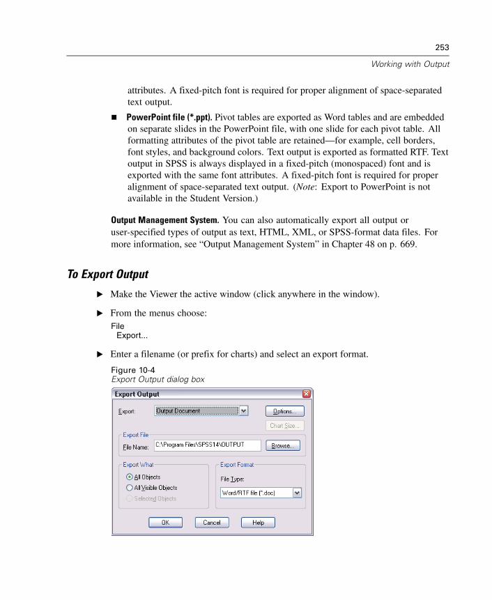
253

Working with Output

attributes. A fixed-pitch font is required for proper alignment of space-separatedtext output.

PowerPoint file (*.ppt). Pivot tables are exported as Word tables and are embeddedon separate slides in the PowerPoint file, with one slide for each pivot table. Allformatting attributes of the pivot table are retained—for example, cell borders,font styles, and background colors. Text output is exported as formatted RTF. Textoutput in SPSS is always displayed in a fixed-pitch (monospaced) font and isexported with the same font attributes. A fixed-pitch font is required for properalignment of space-separated text output. (Note: Export to PowerPoint is notavailable in the Student Version.)

Output Management System. You can also automatically export all output oruser-specified types of output as text, HTML, XML, or SPSS-format data files. Formore information, see “Output Management System” in Chapter 48 on p. 669.

To Export Output

E Make the Viewer the active window (click anywhere in the window).


Export...

E Enter a filename (or prefix for charts) and select an export format.

Figure 10-4Export Output dialog box

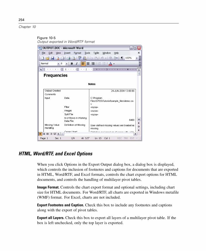
254

Chapter 10

Figure 10-5Output exported in Word/RTF format

HTML, Word/RTF, and Excel Options

When you click Options in the Export Output dialog box, a dialog box is displayed,which controls the inclusion of footnotes and captions for documents that are exportedin HTML, Word/RTF, and Excel formats, controls the chart export options for HTMLdocuments, and controls the handling of multilayer pivot tables.

Image Format. Controls the chart export format and optional settings, including chartsize for HTML documents. For Word/RTF, all charts are exported in Windows metafile(WMF) format. For Excel, charts are not included.

Export Footnotes and Caption. Check this box to include any footnotes and captionsalong with the export of pivot tables.

Export all Layers. Check this box to export all layers of a multilayer pivot table. If thebox is left unchecked, only the top layer is exported.

255

Working with Output

To Set HTML, Word/RTF, and Excel Export Options



Export...

E Select HTML file or Word/RTF file or Excel file as the export format.

E Click Options.

PowerPoint Options

PowerPoint Options controls the inclusion of titles for slides, the inclusion of footnotesand captions for pivot tables, the handling of multilayer pivot tables, and the optionsfor charts exported to PowerPoint. (Note: Export to PowerPoint is not available in theStudent Version.)

Figure 10-6PowerPoint Options dialog box

Include Title on Slide. Check this box to include a title on each slide that is created bythe export. Each slide contains a single item that is exported from the Viewer. The titleis formed from the outline entry for the item in the outline pane of the Viewer.

Export Footnotes and Caption. Check this box to include any footnotes and captionsalong with the export of pivot tables.

Export All Layers. Check this box to export all layers of a multilayer pivot table; eachlayer is placed on a separate slide, and all layers have the same title. If this box is leftunchecked, only the top layer is exported.

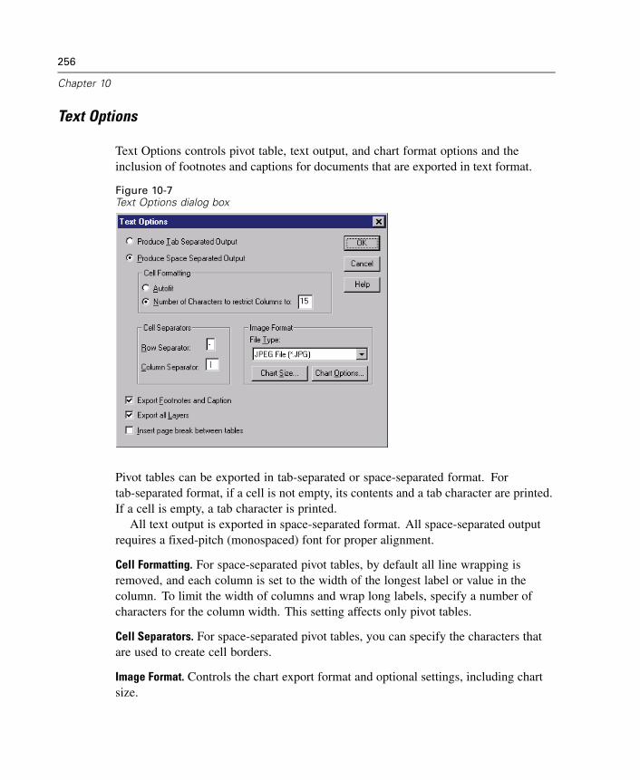
256

Chapter 10

Text Options

Text Options controls pivot table, text output, and chart format options and theinclusion of footnotes and captions for documents that are exported in text format.

Figure 10-7Text Options dialog box

Pivot tables can be exported in tab-separated or space-separated format. Fortab-separated format, if a cell is not empty, its contents and a tab character are printed.If a cell is empty, a tab character is printed.

All text output is exported in space-separated format. All space-separated outputrequires a fixed-pitch (monospaced) font for proper alignment.

Cell Formatting. For space-separated pivot tables, by default all line wrapping isremoved, and each column is set to the width of the longest label or value in thecolumn. To limit the width of columns and wrap long labels, specify a number ofcharacters for the column width. This setting affects only pivot tables.

Cell Separators. For space-separated pivot tables, you can specify the characters thatare used to create cell borders.

Image Format. Controls the chart export format and optional settings, including chartsize.

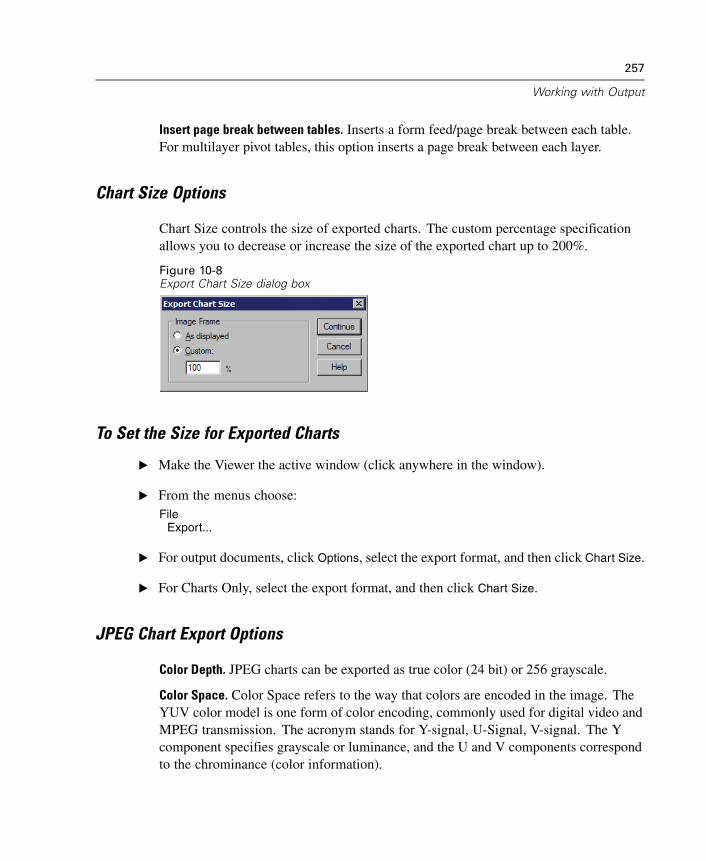
257

Working with Output

Insert page break between tables. Inserts a form feed/page break between each table.For multilayer pivot tables, this option inserts a page break between each layer.

Chart Size Options

Chart Size controls the size of exported charts. The custom percentage specificationallows you to decrease or increase the size of the exported chart up to 200%.

Figure 10-8Export Chart Size dialog box

To Set the Size for Exported Charts



Export...

E For output documents, click Options, select the export format, and then click Chart Size.

E For Charts Only, select the export format, and then click Chart Size.

JPEG Chart Export Options

Color Depth. JPEG charts can be exported as true color (24 bit) or 256 grayscale.

Color Space. Color Space refers to the way that colors are encoded in the image. TheYUV color model is one form of color encoding, commonly used for digital video andMPEG transmission. The acronym stands for Y-signal, U-Signal, V-signal. The Ycomponent specifies grayscale or luminance, and the U and V components correspondto the chrominance (color information).

258

Chapter 10

The ratios represent the sampling rates for each component. Reducing the U and Vsampling rates reduces file size (and also quality). Color Space determines the degreeof “lossiness” for colors in the exported image. YUV 4:4:4 is lossless, while YUV4:2:2 and YUV 4:1:1 represent the decreasing trade-off between file size (disk space)and quality of the colors that are represented.

Progressive encoding. Enables the image to load in stages, initially displaying at lowresolution and then increasing in quality as the image continues to load.

Compression Quality Setting. Controls the ratio of compression to image quality. Thehigher the image quality, the larger the exported file size.

Color Operations. The following operations are available:

Invert. Each pixel is saved as the inverse of the original color.

Gamma correction. Adjusts the intensity of colors in the exported chart by changingthe gamma constant that is used to map the intensity values. Basically, this featurecan be used to lighten or darken the bitmapped image. The value can range from0.10 (darkest) to 6.5 (lightest).

BMP and PICT Chart Export Options

Color Depth. Determines the number of colors in the exported chart. A chart that issaved under any depth will have a minimum of the number of colors that are actuallyused and a maximum of the number of colors that are allowed by the depth. Forexample, if the chart contains three colors—red, white, and black—and you save it as16 colors, the chart will remain as 3 colors.

If the number of colors in the chart exceeds the number of colors for that depth, thecolors will be dithered to replicate the colors in the chart.

Current screen depth is the number of colors that are currently displayed on yourcomputer monitor.




259

Working with Output

Use RLE compression. (BMP only.) A lossless compression technique supported bycommon Windows file formats. Lossless compression means that image quality hasnot been sacrificed for the sake of smaller files.

PNG and TIFF Chart Export Options

Color Depth. Determines the number of colors in the exported chart. A chart that issaved under any depth will have a minimum of the number of colors that are actuallyused and a maximum of the number of colors that are allowed by the depth. Forexample, if the chart contains three colors—red, white, and black—and you save it as16 colors, the chart will remain as 3 colors.

If the number of colors in the chart exceeds the number of colors for that depth, thecolors will be dithered to replicate the colors in the chart.

Current screen depth is the number of colors currently displayed on your computermonitor.




Transparency. Allows you to select a color that will appear transparent in the exportedchart. The feature is available only with 32-bit true color export. Enter integer valuesbetween 0 and 255 for each color. The default value for each color is 255, creating adefault transparent color of white.

Format. (TIFF only) Allows you to set the color space and compress the exportedchart. All color depths are available with RGB color. Only 24- and 32-bit true color isavailable with CMYK. With the YCbCr option, only 24-bit true color is available.

260

Chapter 10

EPS Chart Export Options

Maps, Trees, and Interactive Charts

For trees (Classification Trees option), maps (Maps option), and interactive charts(Graphs menu, Interactive submenu), the following EPS options are available:

Image Preview. Allows you to save a preview image within the EPS image. A previewimage is used mainly when an EPS file is placed within another document. Manyapplications cannot display an EPS image on screen but can display the previewthat is saved with the image. The preview image can be either WMF (smaller andmore scalable) or TIFF (more portable and supported by other platforms). Check theapplication in which you want to include the EPS graphic to see what preview formatthe application supports.

Fonts. Controls the treatment of TrueType fonts in EPS images.

Embed as native TrueType. Embeds most of the font data into the EPS. The resultingPostScript font is called a Type 42 font. Note: Not all PostScript printers haveLevel 3 drivers that can read Type 42 fonts.

Convert to PostScript fonts. Converts TrueType fonts to PostScript (Type 1) fontsbased on font family. For example, Times New Roman is converted to Times,and Arial is converted to Helvetica. Note: This format is not recommended forinteractive graphics that use the SPSS marker font (for example, scatterplots),because there are no meaningful PostScript equivalents for the SPSS TrueTypemarker symbols.

Replace fonts with curves. Turns TrueType fonts into PostScript curve data. Thetext itself is no longer editable as text in applications that can edit EPS graphics.There is also a loss of quality, but this option is useful if you have a PostScriptprinter that doesn’t support Type 42 fonts, and you need to preserve specialTrueType symbols, such as the markers that are used in interactive scatterplots.

Other Charts

For all other charts, the following EPS options are available:

Include TIFF preview. Saves a preview with the EPS image in TIFF format for display inapplications that cannot display EPS images on screen.

261

Working with Output

Fonts. Controls the treatment of fonts in EPS images.

Replace fonts with curves. Turns fonts into PostScript curve data. The text itself isno longer editable as text in applications that can edit EPS graphics. This option isuseful if the fonts that are used in the chart are not available on the output device.

Use font references. If the fonts that are used in the chart are available on the outputdevice, the fonts are used. Otherwise, the output device uses alternate fonts.

WMF Chart Export Options

Aldus placeable. Provides a degree of device independence (same physical size whenopened at 96 dpi versus 120 dpi), but not all applications support this format.

Standard Windows. Supported by most applications that can display Windows metafiles.

To Set Chart Export Options



Export...

E For output documents, click Options, select the export format, and then click Chart

Options.

E For Charts Only, select the export format, and then click Options.

Viewer Printing

There are two options for printing the contents of the Viewer window:

All visible output. Prints only items that are currently displayed in the contents pane.Hidden items (items with a closed book icon in the outline pane or hidden in collapsedoutline layers) are not printed.

Selection. Prints only items that are currently selected in the outline and/or contentspanes.

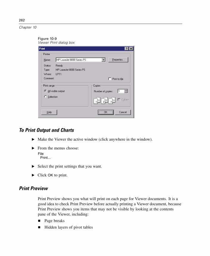
262

Chapter 10

Figure 10-9Viewer Print dialog box

To Print Output and Charts



Print...

E Select the print settings that you want.

E Click OK to print.

Print Preview

Print Preview shows you what will print on each page for Viewer documents. It is agood idea to check Print Preview before actually printing a Viewer document, becausePrint Preview shows you items that may not be visible by looking at the contentspane of the Viewer, including:

Page breaks

Hidden layers of pivot tables

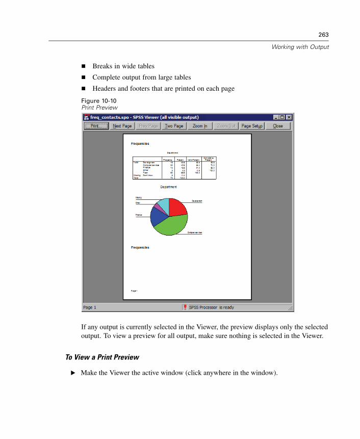
263

Working with Output

Breaks in wide tables

Complete output from large tables

Headers and footers that are printed on each page

Figure 10-10Print Preview

If any output is currently selected in the Viewer, the preview displays only the selectedoutput. To view a preview for all output, make sure nothing is selected in the Viewer.

To View a Print Preview


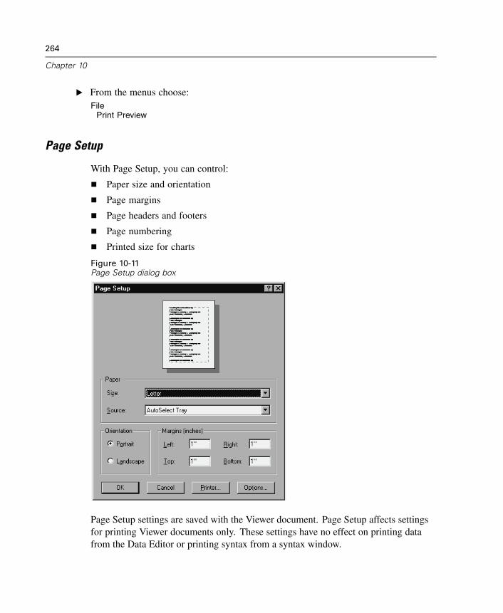
264

Chapter 10


Print Preview

Page Setup

With Page Setup, you can control:

Paper size and orientation

Page margins

Page headers and footers

Page numbering

Printed size for charts

Figure 10-11Page Setup dialog box

Page Setup settings are saved with the Viewer document. Page Setup affects settingsfor printing Viewer documents only. These settings have no effect on printing datafrom the Data Editor or printing syntax from a syntax window.

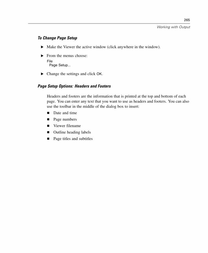
265

Working with Output

To Change Page Setup



Page Setup...

E Change the settings and click OK.

Page Setup Options: Headers and Footers

Headers and footers are the information that is printed at the top and bottom of eachpage. You can enter any text that you want to use as headers and footers. You can alsouse the toolbar in the middle of the dialog box to insert:

Date and time

Page numbers

Viewer filename

Outline heading labels

Page titles and subtitles

266

Chapter 10

Figure 10-12Page Setup Options dialog box, Header/Footer tab

Outline heading labels indicate the first-, second-, third-, and/or fourth-level outlineheading for the first item on each page.

Page titles and subtitles print the current page titles and subtitles. Page titles andsubtitles are created with New Page Title on the Viewer Insert menu or the TITLEand SUBTITLE commands in command syntax. If you have not specified any pagetitles or subtitles, this setting is ignored.

Note: Font characteristics for new page titles and subtitles are controlled on the Viewertab of the Options dialog box (accessed by choosing Options on the Edit menu). Fontcharacteristics for existing page titles and subtitles can be changed by editing thetitles in the Viewer.

To see how your headers and footers will look on the printed page, choose PrintPreview from the File menu.

267

Working with Output

Page Setup Options: Options

This dialog box controls the printed chart size, the space between printed output items,and page numbering.

Printed Chart Size. Controls the size of the printed chart relative to the defined pagesize. The chart’s aspect ratio (width-to-height ratio) is not affected by the printed chartsize. The overall printed size of a chart is limited by both its height and width. Whenthe outer borders of a chart reach the left and right borders of the page, the chart sizecannot increase further to fill additional page height.

Space between items. Controls the space between printed items. Each pivot table,chart, and text object is a separate item. This setting does not affect the display ofitems in the Viewer.

Number pages starting with. Numbers pages sequentially, starting with the specifiednumber.

Figure 10-13Page Setup Options dialog box, Options tab

268

Chapter 10

Saving Output

The contents of the Viewer can be saved to a Viewer document. The saved documentincludes both panes of the Viewer window (the outline and the contents).

To Save a Viewer Document

E From the Viewer window menus choose:File

Save

E Enter the name of the document, and then click Save.

To save results in external formats (for example, HTML or text), use Export on the Filemenu. (This feature is not available in the standalone SmartViewer.)

Save With Password Option

Save With Password allows you to password-protect your Viewer files.

Password. The password is case-sensitive and can be up to 16 characters. If you assigna password, the file cannot be viewed without entering the password.

OEM Code. Leave this field blank unless you have a contractual agreement with SPSSInc. to redistribute the SmartViewer. The OEM license code is provided with thecontract.

To Save Viewer Files with a Password

E From the Viewer window menus choose:File

Save with Password...

E Enter the password.

E Reenter the password to confirm it, and then click OK.

E Enter a filename in the Save As dialog box.

E Click Save.

269

Working with Output

Note: Leave the OEM Code field blank unless you have a contractual agreement withSPSS Inc. to redistribute the SmartViewer.

Chapter

11Draft Viewer

The Draft Viewer provides results in draft form, including:

Simple text output (instead of pivot tables)

Charts as metafile pictures (instead of chart objects)

Text output in the Draft Viewer can be edited, charts can be resized, and both textoutput and charts can be pasted into other applications. However, charts cannot beedited, and the interactive features of pivot tables and charts are not available.

271

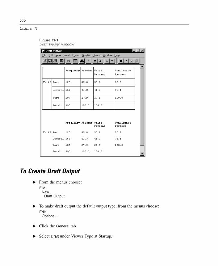
272

Chapter 11

Figure 11-1Draft Viewer window

To Create Draft Output


NewDraft Output

E To make draft output the default output type, from the menus choose:Edit

Options...

E Click the General tab.

E Select Draft under Viewer Type at Startup.

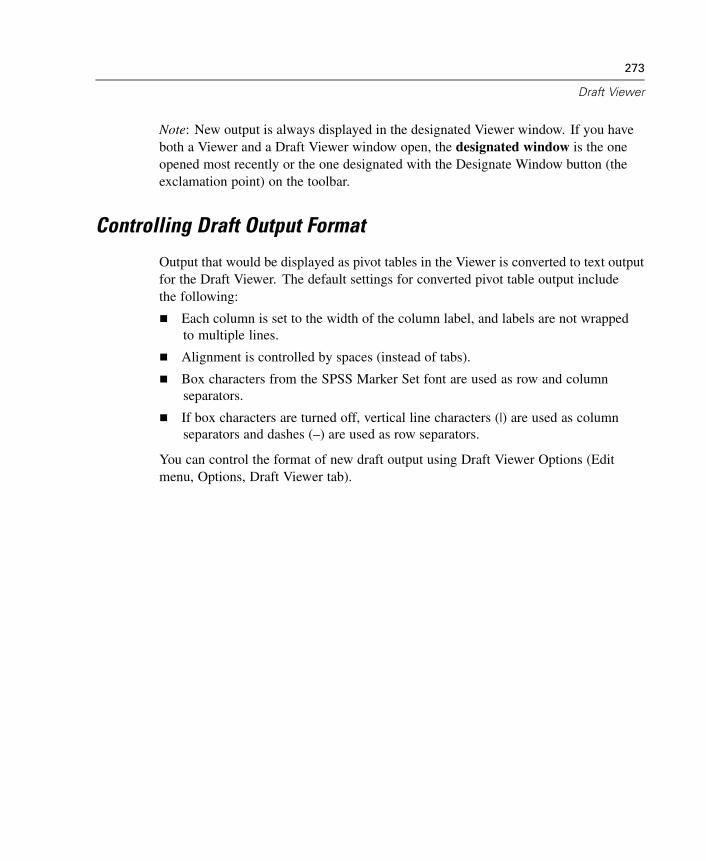
273

Draft Viewer

Note: New output is always displayed in the designated Viewer window. If you haveboth a Viewer and a Draft Viewer window open, the designated window is the oneopened most recently or the one designated with the Designate Window button (theexclamation point) on the toolbar.

Controlling Draft Output Format

Output that would be displayed as pivot tables in the Viewer is converted to text outputfor the Draft Viewer. The default settings for converted pivot table output includethe following:

Each column is set to the width of the column label, and labels are not wrappedto multiple lines.

Alignment is controlled by spaces (instead of tabs).

Box characters from the SPSS Marker Set font are used as row and columnseparators.

If box characters are turned off, vertical line characters (|) are used as columnseparators and dashes (–) are used as row separators.

You can control the format of new draft output using Draft Viewer Options (Editmenu, Options, Draft Viewer tab).

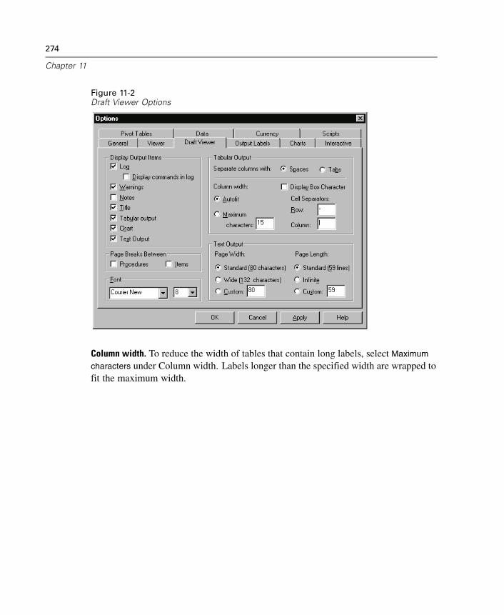
274

Chapter 11

Figure 11-2Draft Viewer Options

Column width. To reduce the width of tables that contain long labels, select Maximum

characters under Column width. Labels longer than the specified width are wrapped tofit the maximum width.

275

Draft Viewer

Figure 11-3Draft output before and after setting maximum column width

Row and column separators. As an alternative to box characters for row and columnborders, you can use the Cell Separators settings to control the row and columnseparators displayed in new draft output. You can specify different cell separators orenter blank spaces if you don’t want any characters used to mark rows and columns.You must deselect Display Box Character to specify cell separators.

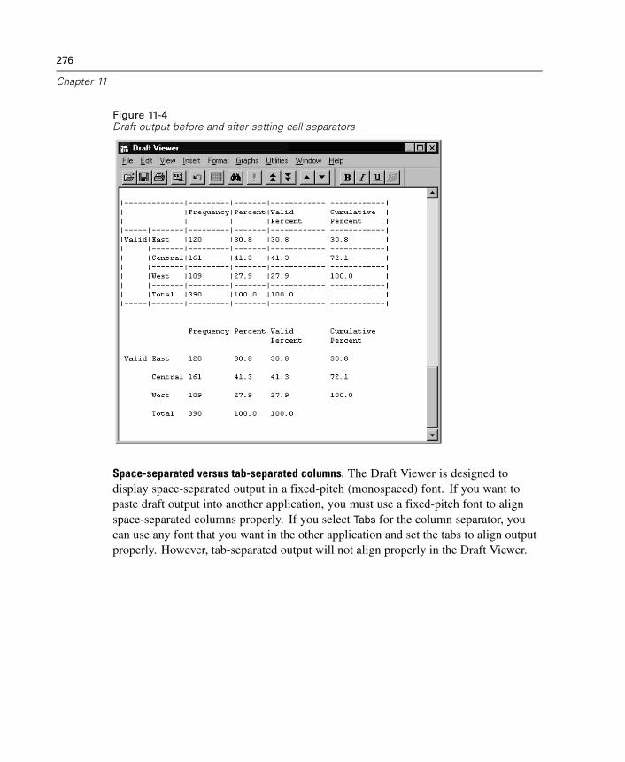
276

Chapter 11

Figure 11-4Draft output before and after setting cell separators

Space-separated versus tab-separated columns. The Draft Viewer is designed todisplay space-separated output in a fixed-pitch (monospaced) font. If you want topaste draft output into another application, you must use a fixed-pitch font to alignspace-separated columns properly. If you select Tabs for the column separator, youcan use any font that you want in the other application and set the tabs to align outputproperly. However, tab-separated output will not align properly in the Draft Viewer.

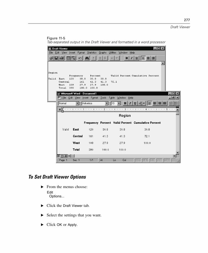
277

Draft Viewer

Figure 11-5Tab-separated output in the Draft Viewer and formatted in a word processor

To Set Draft Viewer Options


Options...

E Click the Draft Viewer tab.

E Select the settings that you want.

E Click OK or Apply.

278

Chapter 11

Draft Viewer output display options affect only new output produced after you changethe settings. Output already displayed in the Draft Viewer is not affected by changes inthese settings.

Fonts in Draft Output

You can modify the font attributes (such as font, size, and style) of text output in theDraft Viewer. However, if you use box characters for row and column borders, propercolumn alignment for space-separated text requires a fixed-pitch (monospaced) font,such as Courier. Additionally, other font changes, such as size and style (for example,bold and italic), applied to only part of a table can affect column alignment.

Row and column borders. The default solid-line row and column borders use theSPSS Marker Set font. The line-drawing characters used to draw the borders are notsupported by other fonts.

To Change Fonts in Draft Viewer

E Select the text to which you want to apply the font change.

E From the Draft Viewer menus choose:Format

Font...

E Select the font attributes that you want to apply to the selected text.

To Print Draft OutputE From the Draft Viewer menus choose:

FilePrint...

To Print Only a Selected Portion of the Draft Output

E Select the output that you want to print.


Print...

279

Draft Viewer

E Select Selection.

Draft Viewer Print Preview

Print Preview shows you what will print on each page for draft documents. It is usuallya good idea to check Print Preview before actually printing a Viewer document becausePrint Preview shows you items that may not fit on the page, including:

Long tables

Wide tables produced by converted pivot table output without column-width control

Text output created with the Wide page-width option (Draft Viewer Options) withthe printer set to Portrait mode

Output that is too wide for the page is truncated, not printed on another page. There areseveral things that you can do to prevent wide output from being truncated:

Use a smaller font size (Format menu, Fonts).

Select Landscape for the page orientation (File menu, Page Setup).

For new output, specify a narrow maximum column width (Edit menu, Options,Draft Viewer tab).

For long tables, use page breaks (Insert menu, Page Break) to control where the tablebreaks between pages.

To View Draft Viewer Print Preview

E From the Draft Viewer menus choose:File

Print Preview

To Save Draft Viewer OutputE From the Draft Viewer menus choose:

FileSave

Draft Viewer output is saved in rich text format (RTF).

280

Chapter 11

To Save Draft Output as Text

E From the Draft Viewer menus choose:File

Export...

You can export all text or just the selected text. Only text output (converted pivot tableoutput and text output) is saved in the exported files; charts are not included.

Chapter

12Pivot Tables

Many of the results in the Viewer are presented in tables that can be pivotedinteractively. That is, you can rearrange the rows, columns, and layers.

Manipulating a Pivot Table

Options for manipulating a pivot table include:

Transposing rows and columns

Moving rows and columns

Creating multidimensional layers

Grouping and ungrouping rows and columns

Showing and hiding cells

Rotating row and column labels

Finding definitions of terms

To Edit a Pivot Table

E Double-click the table.

This activates the Pivot Table Editor.

To Edit Two or More Pivot Tables at a Time

E Right-click the pivot table.

E From the context menu choose:SPSS Pivot Table Object

Open

281

282

Chapter 12

E Repeat the process for each pivot table that you want to edit.

Each pivot table is ready to edit in its own separate window.

To Pivot a Table by Using Icons

E Activate the pivot table.

E From the Pivot Table menus choose:Pivot

Pivoting Trays

E Place the pointer over each icon to see a ToolTip that tells you which table dimensionthe icon represents.

E Drag an icon from one tray to another tray.

Figure 12-1Pivoting trays

This changes the arrangement of the table. For example, suppose that the iconrepresents a variable with categories Yes and No. If you drag the icon from the Rowtray to the Column tray, Yes and No become column labels. Before the move, Yes

and No were row labels.

To Identify Pivot Table Dimensions


E If pivoting trays are not on, from the Pivot Table menus choose:Pivot

Pivoting Trays

283

Pivot Tables

E Click and hold down the mouse button on an icon.

This highlights the dimension labels in the pivot table.

To Transpose Rows and Columns


Transpose Rows and Columns

This has the same effect as dragging all of the row icons into the Column tray anddragging all of the column icons into the Row tray.

To Change Display Order

The order of pivot icons in a dimension tray reflects the display order of elements inthe pivot table. To change the display order of elements in a dimension:


E If pivoting trays are not already on, from the Pivot Table menus choose:Pivot

Pivoting Trays

E Drag the icons in each tray to the order that you want (left to right or top to bottom).

To Move Rows and Columns in a Pivot Table


E Click the label for the row or column you want to move.

E Drag the label to the new position.

E From the context menu choose Insert Before or Swap.

Note: Make sure that Drag to Copy on the Edit menu is not enabled (checked). If Dragto Copy is enabled, deselect it.

284

Chapter 12

To Group Rows or Columns and Insert Group Labels


E Select the labels for the rows or columns that you want to group together (click anddrag or Shift-click to select multiple labels).


Group

A group label is automatically inserted. Double-click the group label to edit the labeltext.

Figure 12-2Row and column groups and labels

Column Group Label

Row Group Label

Clerical

ManagerCustodial

Female Male Total206

10

157 3632774

2784

Note: To add rows or columns to an existing group, you must first ungroup the itemsthat are currently in the group; then you can create a new group that includes theadditional items.

To Ungroup Rows or Columns and Remove Group Labels


E Click anywhere in the group label for the rows or columns that you want to ungroup.


Ungroup

Ungrouping automatically deletes the group label.

To Rotate Pivot Table Labels


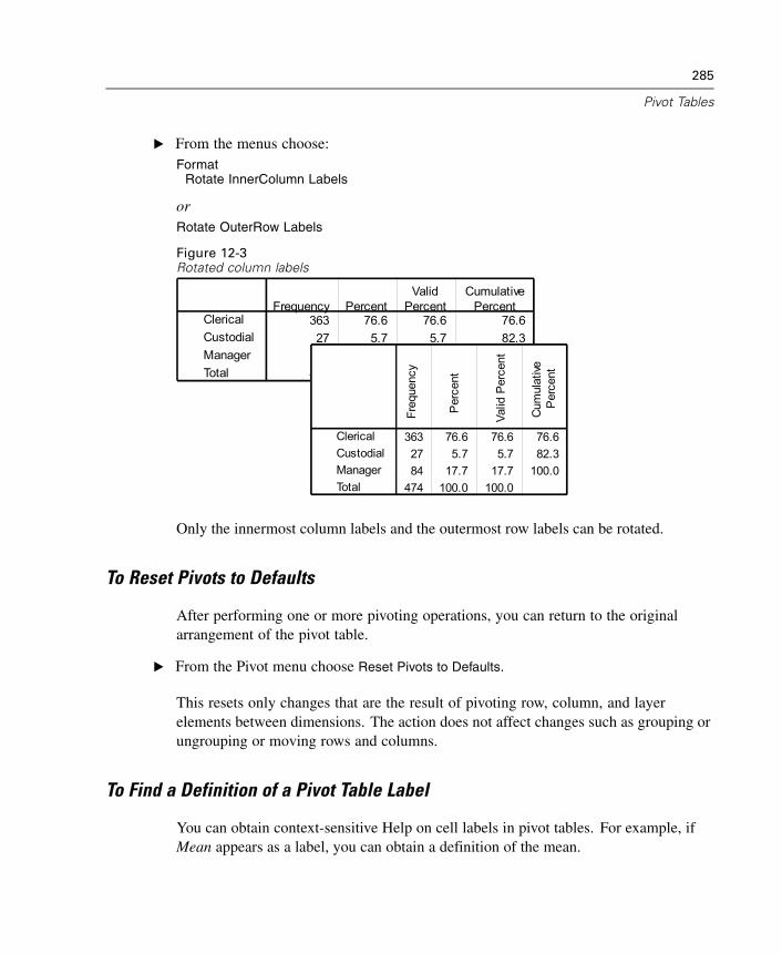
285

Pivot Tables


Rotate InnerColumn Labels

orRotate OuterRow Labels

Figure 12-3Rotated column labels

363 76.6 76.6 76.627 5.7 5.7 82.384 17.7 17.7 100.0

474 100.0 100.0

ClericalCustodialManagerTotal

Frequency PercentValid

PercentCumulative

Percent

363 76.6 76.6 76.627 5.7 5.7 82.384 17.7 17.7 100.0

474 100.0 100.0

ClericalCustodialManagerTotal

Freq

uenc

y

Per

cent

Valid

Per

cent

Cum

ulat

iveP

erce

nt

Only the innermost column labels and the outermost row labels can be rotated.

To Reset Pivots to Defaults

After performing one or more pivoting operations, you can return to the originalarrangement of the pivot table.

E From the Pivot menu choose Reset Pivots to Defaults.

This resets only changes that are the result of pivoting row, column, and layerelements between dimensions. The action does not affect changes such as grouping orungrouping or moving rows and columns.

To Find a Definition of a Pivot Table Label

You can obtain context-sensitive Help on cell labels in pivot tables. For example, ifMean appears as a label, you can obtain a definition of the mean.

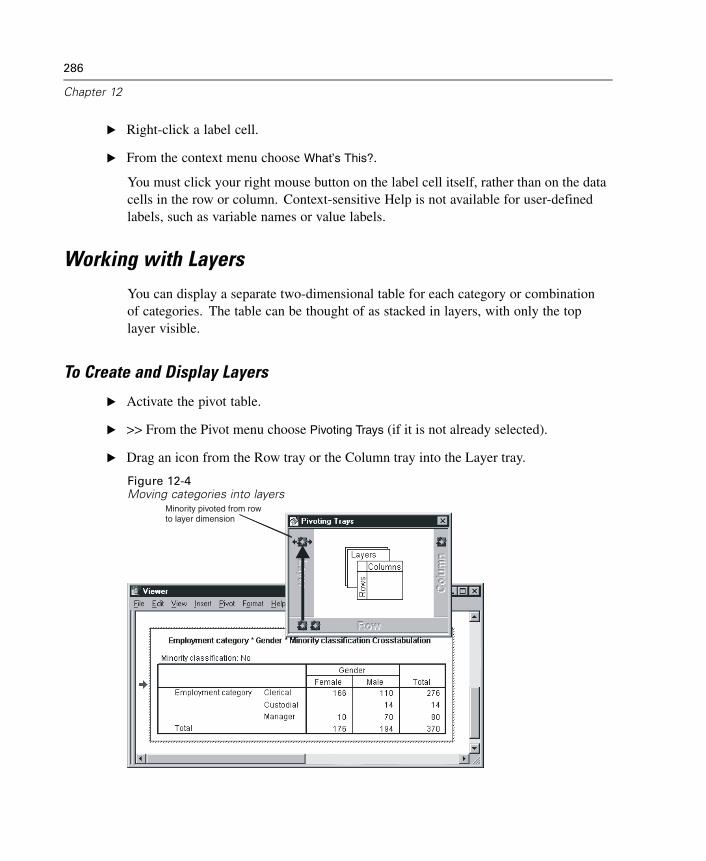
286

Chapter 12

E Right-click a label cell.

E From the context menu choose What’s This?.

You must click your right mouse button on the label cell itself, rather than on the datacells in the row or column. Context-sensitive Help is not available for user-definedlabels, such as variable names or value labels.

Working with LayersYou can display a separate two-dimensional table for each category or combinationof categories. The table can be thought of as stacked in layers, with only the toplayer visible.

To Create and Display Layers


E >> From the Pivot menu choose Pivoting Trays (if it is not already selected).

E Drag an icon from the Row tray or the Column tray into the Layer tray.

Figure 12-4Moving categories into layers

Minority pivoted from row to layer dimension

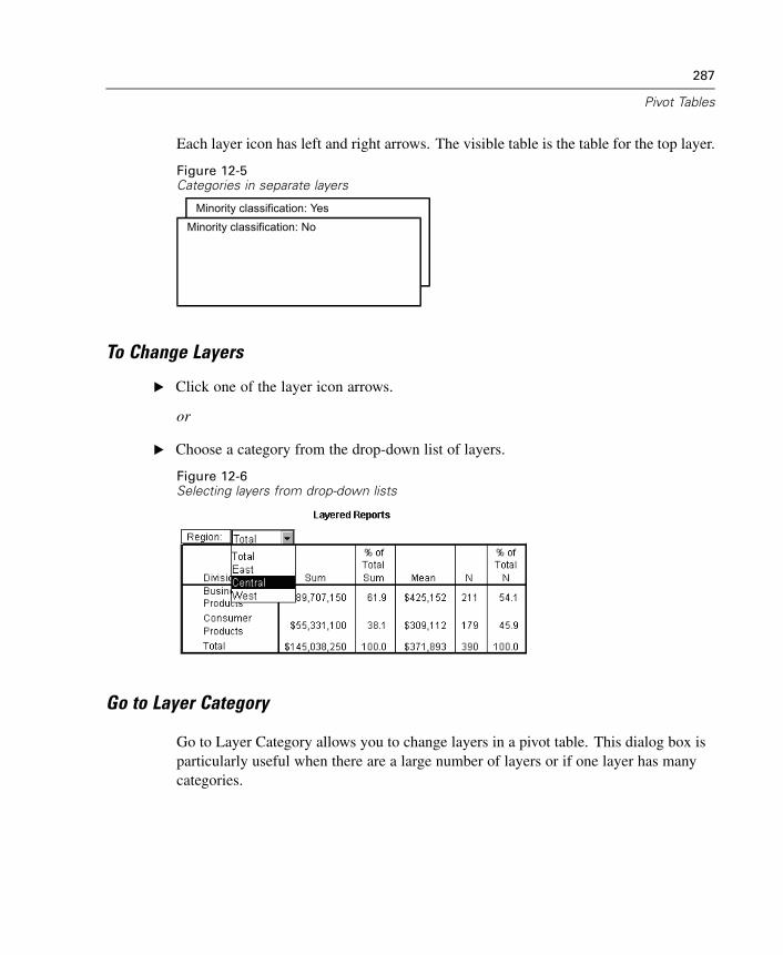
287

Pivot Tables

Each layer icon has left and right arrows. The visible table is the table for the top layer.

Figure 12-5Categories in separate layers

Minority classification: YesMinority classification: No

To Change Layers

E Click one of the layer icon arrows.

or

E Choose a category from the drop-down list of layers.

Figure 12-6Selecting layers from drop-down lists

Go to Layer Category

Go to Layer Category allows you to change layers in a pivot table. This dialog box isparticularly useful when there are a large number of layers or if one layer has manycategories.

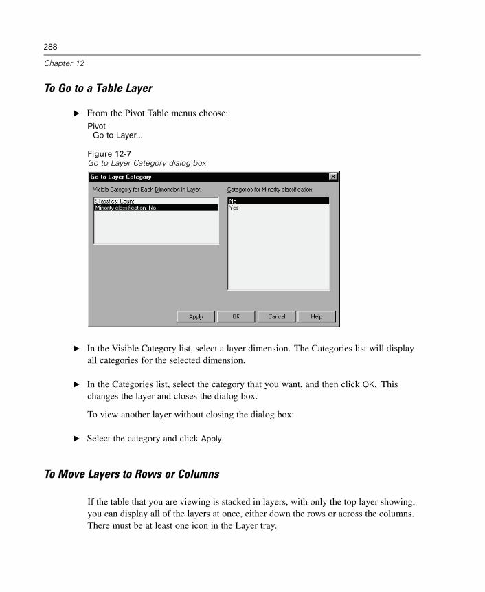
288

Chapter 12

To Go to a Table Layer


Go to Layer...

Figure 12-7Go to Layer Category dialog box

E In the Visible Category list, select a layer dimension. The Categories list will displayall categories for the selected dimension.

E In the Categories list, select the category that you want, and then click OK. Thischanges the layer and closes the dialog box.

To view another layer without closing the dialog box:

E Select the category and click Apply.

To Move Layers to Rows or Columns

If the table that you are viewing is stacked in layers, with only the top layer showing,you can display all of the layers at once, either down the rows or across the columns.There must be at least one icon in the Layer tray.

289

Pivot Tables

E From the Pivot menu choose Move Layers to Rows.

or

E From the Pivot menu choose Move Layers to Columns.

You can also move layers to rows or columns by dragging their icons between theLayer, Row, and Column pivoting trays.

Bookmarks

Bookmarks allow you to save different views of a pivot table. Bookmarks save:

Placement of elements in row, column, and layer dimensions

Display order of elements in each dimension

Currently displayed layer for each layer element

To Bookmark Pivot Table Views


E Pivot the table to the view that you want to bookmark.

E From the menus choose:Pivot

Bookmarks…

E Enter a name for the bookmark. (Bookmark names are not case-sensitive.)

E Click Add.

Each pivot table has its own set of bookmarks. Within a pivot table, each bookmarkname must be unique, but you can use duplicate bookmark names in different pivottables.

To Display a Bookmarked Pivot Table View


290

Chapter 12


Bookmarks…

E Click the name of the bookmark in the list.

E Click Go To.

To Rename a Pivot Table Bookmark



Bookmarks…

E Click the name of the bookmark in the list.

E Click Rename.

E Enter the new bookmark name.

E Click OK.

Showing and Hiding Cells

Many types of cells can be hidden, including:

Dimension labels

Categories, including the label cell and data cells in a row or column

Category labels (without hiding the data cells)

Footnotes, titles, and captions

To Hide Rows and Columns in a Table

E Ctrl-Alt-click the category label of the row or column to be hidden.

291

Pivot Tables

E From the Pivot Table menus choose:View

Hide

or

E Right-click the row or column.

E From the context menu choose Hide Category.

To Show Hidden Rows and Columns in a Table

E Select another label that is in the same dimension as the hidden row or column.

For example, if the Female category of the Gender dimension is hidden, click theMale category.


Show All Categories in dimension name

For example, choose Show All Categories in Gender.

or


Show All

This displays all hidden cells in the table. (If Hide empty rows and columns is selectedin Table Properties for this table, a completely empty row or column remains hidden.)

To Hide or Show a Dimension Label


E Select the dimension label or any category label within the dimension.


Hide (or Show) Dimension Label

292

Chapter 12

To Hide or Show a Footnote in a Table

E Select a footnote.


Hide (or Show)

To Hide or Show a Caption or Title in a Table

E Select a caption or title.


Hide (or Show)

Editing Results

The appearance and contents of each table or text output item can be edited. You can:

Apply a TableLook.

Change the properties of the current table.

Change the properties of cells in the table.

Modify text.

Add footnotes and captions to tables.

Add items to the Viewer.

Copy and paste results into other applications.

Modify data cell widths.

Changing the Appearance of Tables

You can change the appearance of a table either by editing table properties or byapplying a TableLook. Each TableLook consists of a collection of table properties,including general appearance, footnote properties, cell properties, and borders. You canselect one of the preset TableLooks, or you can create and save a custom TableLook.

293

Pivot Tables

TableLooks

A TableLook is a set of properties that define the appearance of a table. You can selecta previously defined TableLook or create your own TableLook.

Before or after a TableLook is applied, you can change cell formats for individualcells or groups of cells by using cell properties. The edited cell formats will remainintact, even when you apply a new TableLook.

For example, you might start by applying TableLook 9POINT, then select a datacolumn, and from the Cell Formats dialog box, change to a bold font for that column.Later, you change the TableLook to BOXED. The previously selected column retainsthe bold font while the rest of the characteristics are applied from the BOXEDTableLook.

Optionally, you can reset all cells to the cell formats that are defined by the currentTableLook. This resets any cells that have been edited. If As Displayed is selected inthe TableLook Files list, any edited cells are reset to the current table properties.

To Apply or Save a TableLook

E Activate a pivot table.


TableLooks...

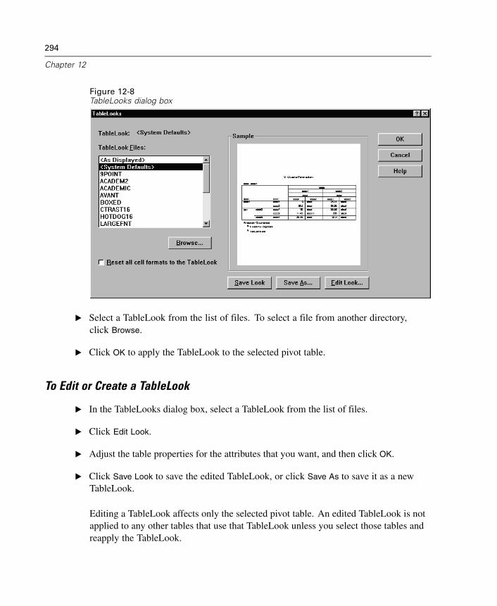
294

Chapter 12

Figure 12-8TableLooks dialog box

E Select a TableLook from the list of files. To select a file from another directory,click Browse.

E Click OK to apply the TableLook to the selected pivot table.

To Edit or Create a TableLook

E In the TableLooks dialog box, select a TableLook from the list of files.

E Click Edit Look.

E Adjust the table properties for the attributes that you want, and then click OK.

E Click Save Look to save the edited TableLook, or click Save As to save it as a newTableLook.

Editing a TableLook affects only the selected pivot table. An edited TableLook is notapplied to any other tables that use that TableLook unless you select those tables andreapply the TableLook.

295

Pivot Tables

Table Properties

The Table Properties dialog box allows you to set general properties of a table, set cellstyles for various parts of a table, and save a set of those properties as a TableLook.Using the tabs on this dialog box, you can:

Control general properties, such as hiding empty rows or columns and adjustingprinting properties.

Control the format and position of footnote markers.

Determine specific formats for cells in the data area, for row and column labels,and for other areas of the table.

Control the width and color of the lines that form the borders of each area of thetable.

To Change Pivot Table PropertiesE Double-click anywhere in the pivot table to activate it.

E From the Pivot Table menus choose:Format

Table Properties...

E Select a tab (General, Footnotes, Cell Formats, Borders, or Printing).

E Select the options that you want.


The new properties are applied to the selected pivot table. To apply new tableproperties to a TableLook instead of just the selected table, edit the TableLook (Formatmenu, TableLooks).

Table Properties: General

Several properties apply to the table as a whole. You can:

Show or hide empty rows and columns. (An empty row or column has nothing inany of the data cells.)

296

Chapter 12

Control the placement of row labels, which can be in the upper left corner or nested.

Control maximum and minimum column width (expressed in points).

Figure 12-9Table Properties dialog box, General tab

To Change General Table Properties

E Click the General tab.



Table Properties: Footnotes

The properties of footnote markers include style and position in relation to text.

The style of footnote markers is either numbers (1, 2, 3, ...) or letters (a, b, c, ...).

The footnote markers can be attached to text as superscripts or subscripts.

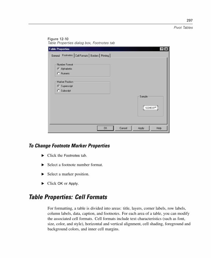
297

Pivot Tables

Figure 12-10Table Properties dialog box, Footnotes tab

To Change Footnote Marker Properties

E Click the Footnotes tab.

E Select a footnote number format.

E Select a marker position.


Table Properties: Cell Formats

For formatting, a table is divided into areas: title, layers, corner labels, row labels,column labels, data, caption, and footnotes. For each area of a table, you can modifythe associated cell formats. Cell formats include text characteristics (such as font,size, color, and style), horizontal and vertical alignment, cell shading, foreground andbackground colors, and inner cell margins.

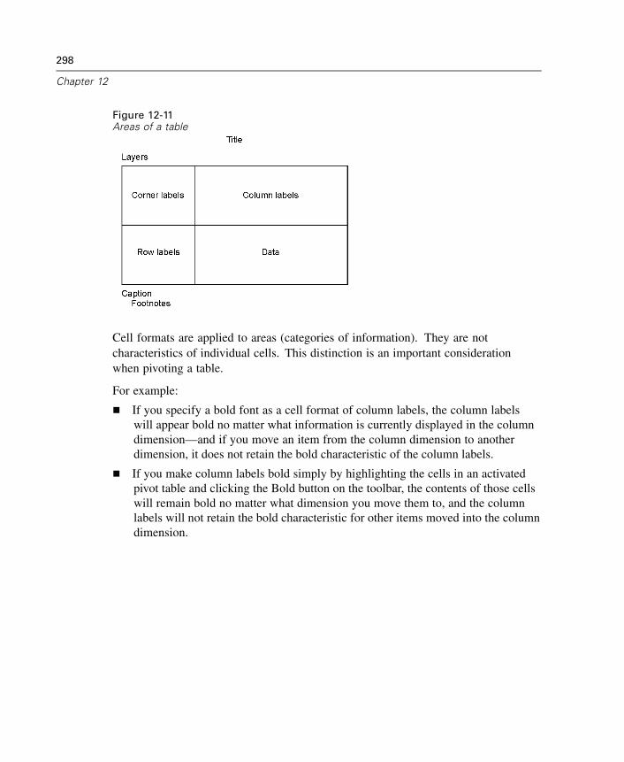
298

Chapter 12

Figure 12-11Areas of a table

Cell formats are applied to areas (categories of information). They are notcharacteristics of individual cells. This distinction is an important considerationwhen pivoting a table.

For example:

If you specify a bold font as a cell format of column labels, the column labelswill appear bold no matter what information is currently displayed in the columndimension—and if you move an item from the column dimension to anotherdimension, it does not retain the bold characteristic of the column labels.

If you make column labels bold simply by highlighting the cells in an activatedpivot table and clicking the Bold button on the toolbar, the contents of those cellswill remain bold no matter what dimension you move them to, and the columnlabels will not retain the bold characteristic for other items moved into the columndimension.

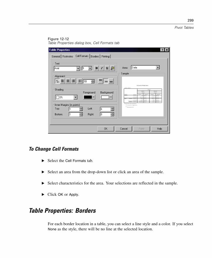
299

Pivot Tables

Figure 12-12Table Properties dialog box, Cell Formats tab

To Change Cell Formats

E Select the Cell Formats tab.

E Select an area from the drop-down list or click an area of the sample.

E Select characteristics for the area. Your selections are reflected in the sample.


Table Properties: Borders

For each border location in a table, you can select a line style and a color. If you selectNone as the style, there will be no line at the selected location.

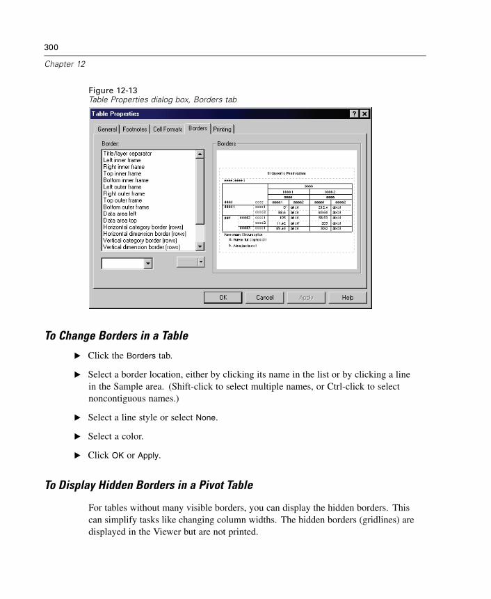
300

Chapter 12

Figure 12-13Table Properties dialog box, Borders tab

To Change Borders in a Table

E Click the Borders tab.

E Select a border location, either by clicking its name in the list or by clicking a linein the Sample area. (Shift-click to select multiple names, or Ctrl-click to selectnoncontiguous names.)

E Select a line style or select None.

E Select a color.


To Display Hidden Borders in a Pivot Table

For tables without many visible borders, you can display the hidden borders. Thiscan simplify tasks like changing column widths. The hidden borders (gridlines) aredisplayed in the Viewer but are not printed.

301

Pivot Tables

E Double-click anywhere in the pivot table to activate it.


Gridlines

Table Properties: Printing

You can control the following properties for printed pivot tables:

Print all layers or only the top layer of the table, and print each layer on a separatepage. (This setting affects only printing, not the display of layers in the Viewer.)

Shrink a table horizontally or vertically to fit the page for printing.

Control widow/orphan lines by controlling the minimum number of rows andcolumns that will be contained in any printed section of a table if the table is toowide and/or too long for the defined page size. (Note: If a table is too long to fit onthe current page because there is other output above it, but it will fit within thedefined page length, the table is automatically printed on a new page, regardlessof the widow/orphan setting.)

Include continuation text for tables that don’t fit on a single page. You can displaycontinuation text at the bottom of each page and at the top of each page. If neitheroption is selected, the continuation text will not be displayed.

To Control Pivot Table Printing

E Click the Printing tab.

E Select the printing options that you want.


Font

A TableLook allows you to specify font characteristics for different areas of the table.You can also change the font for any individual cell. Options for the font in a cellinclude the font face, style, size, and color. You can also hide the text or underline it.

If you specify font properties in a cell, they apply in all of the table layers thathave the same cell.

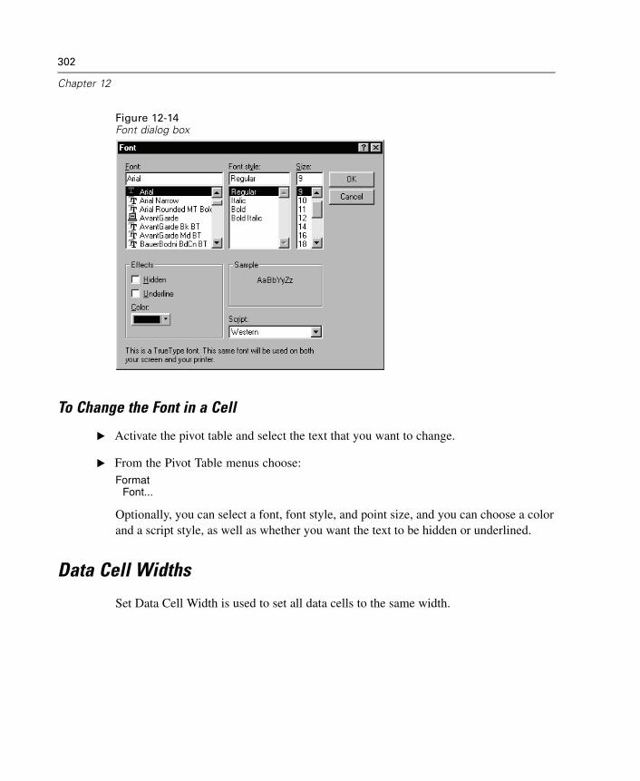
302

Chapter 12

Figure 12-14Font dialog box

To Change the Font in a Cell

E Activate the pivot table and select the text that you want to change.


Font...

Optionally, you can select a font, font style, and point size, and you can choose a colorand a script style, as well as whether you want the text to be hidden or underlined.

Data Cell Widths

Set Data Cell Width is used to set all data cells to the same width.

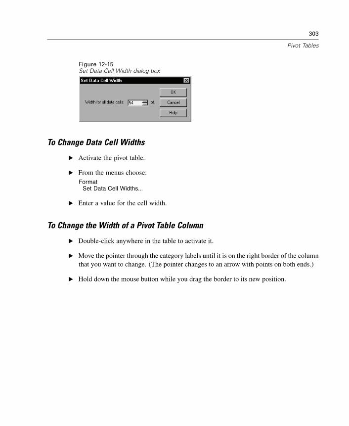
303

Pivot Tables

Figure 12-15Set Data Cell Width dialog box

To Change Data Cell Widths



Set Data Cell Widths...

E Enter a value for the cell width.

To Change the Width of a Pivot Table Column

E Double-click anywhere in the table to activate it.

E Move the pointer through the category labels until it is on the right border of the columnthat you want to change. (The pointer changes to an arrow with points on both ends.)

E Hold down the mouse button while you drag the border to its new position.

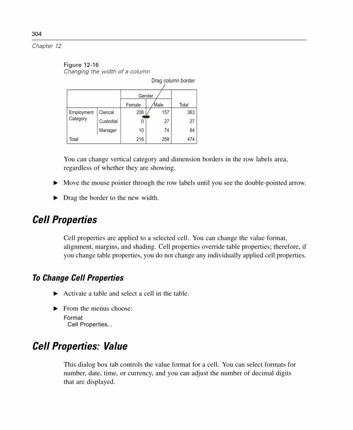
304

Chapter 12

Figure 12-16Changing the width of a column

You can change vertical category and dimension borders in the row labels area,regardless of whether they are showing.

E Move the mouse pointer through the row labels until you see the double-pointed arrow.

E Drag the border to the new width.

Cell Properties

Cell properties are applied to a selected cell. You can change the value format,alignment, margins, and shading. Cell properties override table properties; therefore, ifyou change table properties, you do not change any individually applied cell properties.

To Change Cell Properties

E Activate a table and select a cell in the table.


Cell Properties...

Cell Properties: Value

This dialog box tab controls the value format for a cell. You can select formats fornumber, date, time, or currency, and you can adjust the number of decimal digitsthat are displayed.

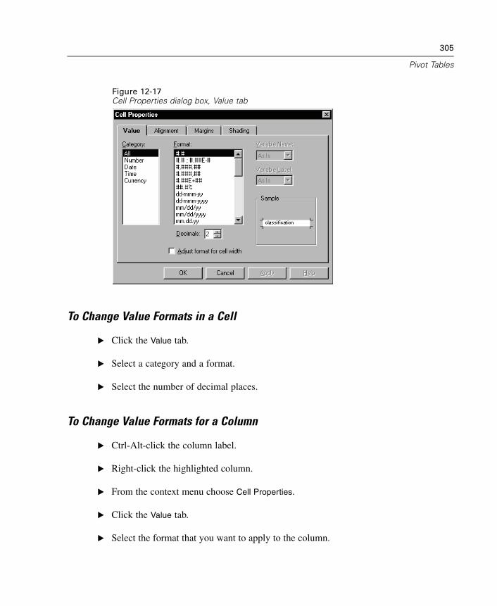
305

Pivot Tables

Figure 12-17Cell Properties dialog box, Value tab

To Change Value Formats in a Cell

E Click the Value tab.

E Select a category and a format.

E Select the number of decimal places.

To Change Value Formats for a Column

E Ctrl-Alt-click the column label.

E Right-click the highlighted column.

E From the context menu choose Cell Properties.

E Click the Value tab.

E Select the format that you want to apply to the column.

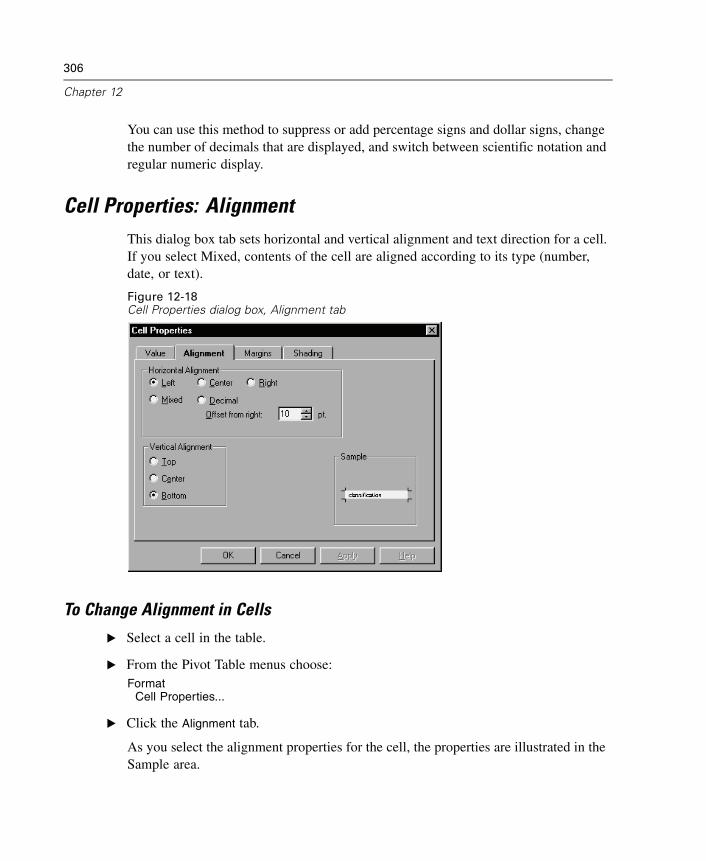
306

Chapter 12

You can use this method to suppress or add percentage signs and dollar signs, changethe number of decimals that are displayed, and switch between scientific notation andregular numeric display.

Cell Properties: AlignmentThis dialog box tab sets horizontal and vertical alignment and text direction for a cell.If you select Mixed, contents of the cell are aligned according to its type (number,date, or text).

Figure 12-18Cell Properties dialog box, Alignment tab

To Change Alignment in Cells

E Select a cell in the table.


Cell Properties...

E Click the Alignment tab.

As you select the alignment properties for the cell, the properties are illustrated in theSample area.

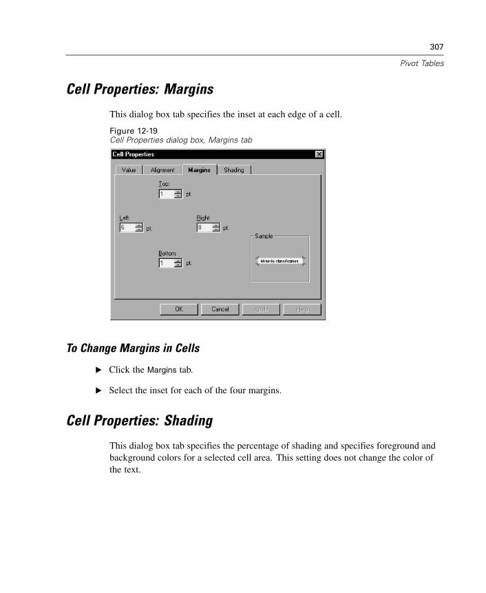
307

Pivot Tables

Cell Properties: Margins

This dialog box tab specifies the inset at each edge of a cell.

Figure 12-19Cell Properties dialog box, Margins tab

To Change Margins in Cells

E Click the Margins tab.

E Select the inset for each of the four margins.

Cell Properties: Shading

This dialog box tab specifies the percentage of shading and specifies foreground andbackground colors for a selected cell area. This setting does not change the color ofthe text.

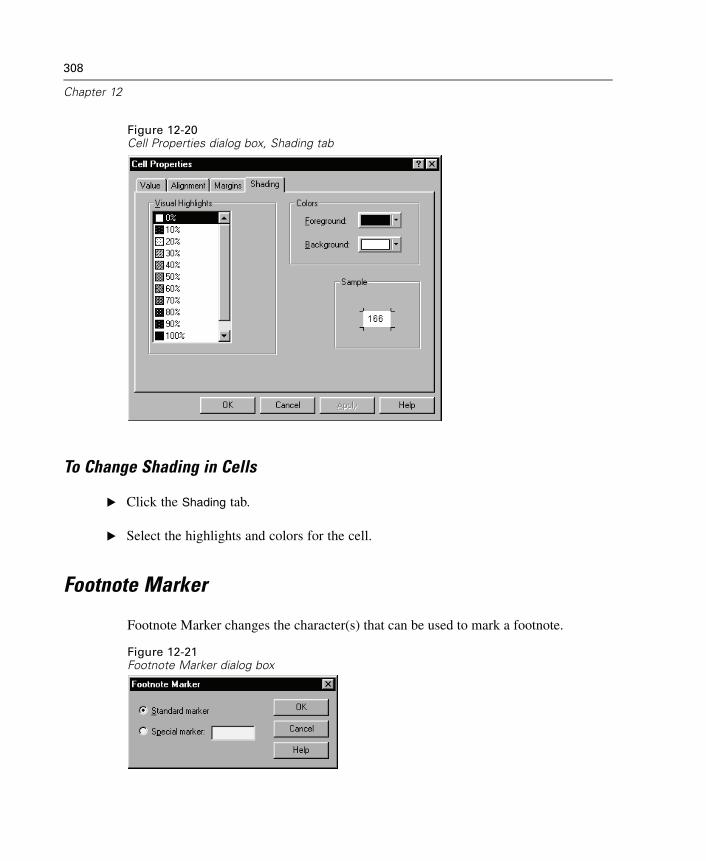
308

Chapter 12

Figure 12-20Cell Properties dialog box, Shading tab

To Change Shading in Cells

E Click the Shading tab.

E Select the highlights and colors for the cell.

Footnote Marker

Footnote Marker changes the character(s) that can be used to mark a footnote.

Figure 12-21Footnote Marker dialog box

309

Pivot Tables

To Change Footnote Marker Characters

E Select a footnote.


Footnote Marker...

E Enter one or two characters.

To Renumber Footnotes

When you have pivoted a table by switching rows, columns, and layers, the footnotesmay be out of order. To renumber the footnotes:



Renumber Footnotes

Selecting Rows and Columns in Pivot TablesIn pivot tables, there are some constraints on how you select entire rows andcolumns, and the visual highlight that indicates the selected row or column may spannoncontiguous areas of the table.

To Select a Row or Column in a Pivot TableE Double-click anywhere in the pivot table to activate it.

E Click a row or column label.


SelectData and Label Cells

or

E Ctrl-Alt-click the row or column label.

310

Chapter 12

If the table contains more than one dimension in the row or column area, thehighlighted selection may span multiple noncontiguous cells.

Modifying Pivot Table Results

Text appears in the Viewer in many items. You can edit the text or add new text. Pivottables can be modified by:

Editing text within pivot table cells

Adding captions and footnotes

To Modify Text in a Cell


E Double-click the cell.

E Edit the text.

E Press Enter to record your changes, or press Esc to revert to the previous contents ofthe cell.

To Add Captions to a Table

E From the Pivot Table menus choose:Insert

Caption

The words Table Caption are displayed at the bottom of the table.

E Double-click the words Table Caption and replace them with your caption text.

To Add a Footnote to a Table

A footnote can be attached to any item in a table.

E Click a title, cell, or caption within an activated pivot table.

311

Pivot Tables

E From the Pivot Table menus choose:Insert

Footnote...

E Double-click the word Footnote and replace it with the footnote text.

Printing Pivot Tables

Several factors can affect the way that printed pivot tables look, and these factors canbe controlled by changing pivot table attributes.

For multidimensional pivot tables (tables with layers), you can either print alllayers or print only the top (visible) layer.

For long or wide pivot tables, you can automatically resize the table to fit the pageor control the location of table breaks and page breaks.

Use Print Preview on the File menu to see how printed pivot tables will look.

To Print Hidden Layers of a Pivot TableE Double-click anywhere in the table to activate it.


Table Properties...

E On the Printing tab, select Print all layers.

You can also print each layer of a pivot table on a separate page.

Controlling Table Breaks for Wide and Long Tables

Pivot tables that are either too wide or too long to print within the defined page size areautomatically split and printed in multiple sections. (For wide tables, multiple sectionswill print on the same page if there is room.) You can:

Control the row and column locations where large tables are split.

Specify rows and columns that should be kept together when tables are split.

Rescale large tables to fit the defined page size.

312

Chapter 12

To Specify Row and Column Breaks for Printed Pivot Tables


E Click the column label to the left of where you want to insert the break, or click therow label above where you want to insert the break.


Break Here

To Specify Rows or Columns to Keep Together


E Select the labels of the rows or columns that you want to keep together. (Click anddrag or Shift-click to select multiple row or column labels.)


Keep Together

To Rescale a Pivot Table to Fit the Page Size



Table Properties

E Click the Printing tab.

E Select Rescale wide table to fit page.

and/or

E Select Rescale long table to fit page.

Chapter

13Working with Command Syntax

SPSS provides a powerful command language that allows you to save and automatemany common tasks. It also provides some functionality not found in the menus anddialog boxes.

Most commands are accessible from the menus and dialog boxes. However, somecommands and options are available only by using the command language. Thecommand language also allows you to save your jobs in a syntax file so that you canrepeat your analysis at a later date or run it in an automated job with the ProductionFacility.

A syntax file is simply a text file that contains commands. While it is possible toopen a syntax window and type in commands, it is often easier if you let the softwarehelp you build your syntax file using one of the following methods:

Pasting command syntax from dialog boxes

Copying syntax from the output log

Copying syntax from the journal file

Detailed command syntax reference information is available in two forms: integratedinto the overall Help system and as a separate PDF file, called the SPSS CommandSyntax Reference, also available from the Help menu.

Context-sensitive Help for the current command in a syntax window is availableby pressing the F1 key.

Syntax Rules

When you run commands from a command syntax window during an SPSS session,you are running commands in interactive mode.

313

314

Chapter 13

The following rules apply to command specifications in interactive mode:

Each command should with a period as a command terminator. It is best to omitthe terminator on BEGIN DATA, however, so that inline data is treated as onecontinuous specification.

The command terminator must be the last nonblank character in a command.

In the absence of a period as the command terminator, a blank line is interpreted asa command terminator.

Commands can begin in any column of a command line and continue for as manylines as needed. The exception is the END DATA command, which must begin inthe first column of the first line after the end of data.

Note: For compatibility with other modes of command execution (including commandfiles run with INSERT or INCLUDE commands in an interactive session), each line ofcommand syntax should not exceed 256 bytes.

Most subcommands are separated by slashes (/). The slash before the firstsubcommand on a command is usually optional.

Variable names must be spelled out fully.

Text included within apostrophes or quotation marks must be contained on a singleline.

A period (.) must be used to indicate decimals, regardless of your regional orlocale settings.

Variable names ending in a period can cause errors in commands created by thedialog boxes. You cannot create such variable names in the dialog boxes, and youshould generally avoid them.

Command syntax is case insensitive, and three- or four-letter abbreviations can be usedfor many command specifications. You can use as many lines as you want to specifya single command. You can add space or break lines at almost any point where asingle blank is allowed, such as around slashes, parentheses, arithmetic operators, orbetween variable names. For example,

FREQUENCIESVARIABLES=JOBCAT GENDER/PERCENTILES=25 50 75/BARCHART.

and

315

Working with Command Syntax

freq var=jobcat gender /percent=25 50 75 /bar.

are both acceptable alternatives that generate the same results.

INCLUDE Files

For command files run via the INCLUDE command, batch mode syntax rules apply.

The following rules apply to command specifications in batch or production mode:

All commands in the command file must begin in column 1. You can use plus(+) or minus (–) signs in the first column if you want to indent the commandspecification to make the command file more readable.

If multiple lines are used for a command, column 1 of each continuation line mustbe blank.

Command terminators are optional.

A line cannot exceed 256 bytes; any additional characters are truncated.

Unless you have existing command files that already use the INCLUDE command,you should probably use the INSERT command instead since it can accommodatecommand files that conform to either set of rules. If you generate command syntaxby pasting dialog box choices into a syntax window, the format of the commandsis suitable for any mode of operation. See the SPSS Command Syntax Reference(available in PDF format from the Help menu) for more information.

Pasting Syntax from Dialog BoxesThe easiest way to build a command syntax file is to make selections in dialog boxesand paste the syntax for the selections into a syntax window. By pasting the syntax ateach step of a lengthy analysis, you can build a job file that allows you to repeat theanalysis at a later date or run an automated job with the Production Facility.

In the syntax window, you can run the pasted syntax, edit it, and save it in a syntaxfile.

To Paste Syntax from Dialog Boxes

E Open the dialog box and make the selections that you want.

E Click Paste.

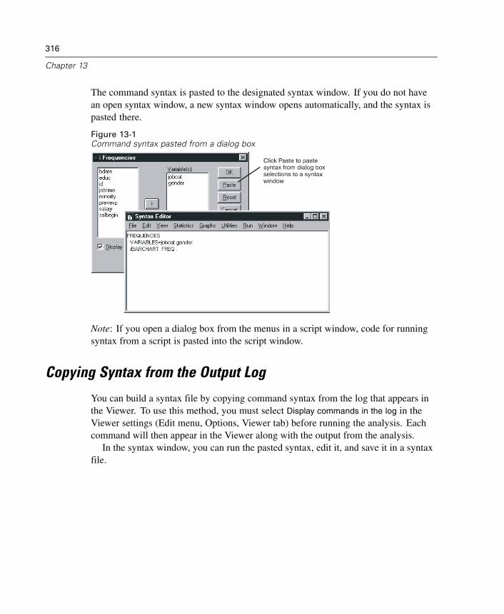
316

Chapter 13

The command syntax is pasted to the designated syntax window. If you do not havean open syntax window, a new syntax window opens automatically, and the syntax ispasted there.

Figure 13-1Command syntax pasted from a dialog box

Note: If you open a dialog box from the menus in a script window, code for runningsyntax from a script is pasted into the script window.

Copying Syntax from the Output Log

You can build a syntax file by copying command syntax from the log that appears inthe Viewer. To use this method, you must select Display commands in the log in theViewer settings (Edit menu, Options, Viewer tab) before running the analysis. Eachcommand will then appear in the Viewer along with the output from the analysis.

In the syntax window, you can run the pasted syntax, edit it, and save it in a syntaxfile.

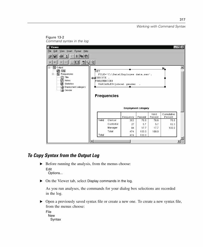
317


Figure 13-2Command syntax in the log

To Copy Syntax from the Output Log

E Before running the analysis, from the menus choose:Edit

Options...

E On the Viewer tab, select Display commands in the log.

As you run analyses, the commands for your dialog box selections are recordedin the log.

E Open a previously saved syntax file or create a new one. To create a new syntax file,from the menus choose:File

NewSyntax

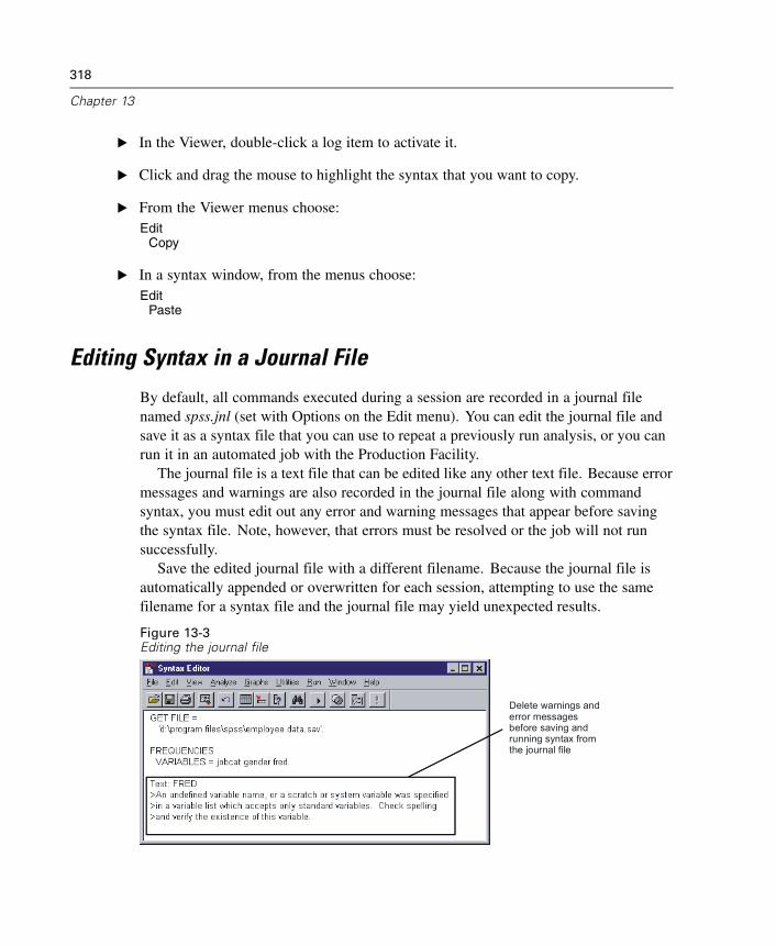
318

Chapter 13

E In the Viewer, double-click a log item to activate it.

E Click and drag the mouse to highlight the syntax that you want to copy.

E From the Viewer menus choose:Edit

Copy

E In a syntax window, from the menus choose:Edit

Paste

Editing Syntax in a Journal File

By default, all commands executed during a session are recorded in a journal filenamed spss.jnl (set with Options on the Edit menu). You can edit the journal file andsave it as a syntax file that you can use to repeat a previously run analysis, or you canrun it in an automated job with the Production Facility.

The journal file is a text file that can be edited like any other text file. Because errormessages and warnings are also recorded in the journal file along with commandsyntax, you must edit out any error and warning messages that appear before savingthe syntax file. Note, however, that errors must be resolved or the job will not runsuccessfully.

Save the edited journal file with a different filename. Because the journal file isautomatically appended or overwritten for each session, attempting to use the samefilename for a syntax file and the journal file may yield unexpected results.

Figure 13-3Editing the journal file

Delete warnings anderror messages before saving andrunning syntax fromthe journal file

319


To Edit Syntax in a Journal File

E To open the journal file, from the menus choose:File

OpenOther...

E Locate and open the journal file (by default, spss.jnl is located in the temp directory).

Select All files (*.*) for Files of Type or enter *.jnl in the File Name text box to displayjournal files in the file list. If you have difficulty locating the file, use Options on theEdit menu to see where the journal is saved in your system.

E Edit the file to remove any error messages or warnings, indicated by the > sign.

E Save the edited journal file using a different filename. (We recommend that you use afilename with the extension .sps, the default extension for syntax files.)

To Run Command Syntax

E Highlight the commands that you want to run in the syntax window.

E Click the Run button (the right-pointing triangle) on the Syntax Editor toolbar.

or

E Select one of the choices from the Run menu.

All. Runs all commands in the syntax window.

Selection. Runs the currently selected commands. This includes any commandspartially highlighted.

Current. Runs the command where the cursor is currently located.

To End. Runs all commands from the current cursor location to the end of thecommand syntax file.

The Run button on the Syntax Editor toolbar runs the selected commands or thecommand where the cursor is located if there is no selection.

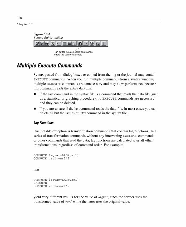
320

Chapter 13

Figure 13-4Syntax Editor toolbar

Multiple Execute CommandsSyntax pasted from dialog boxes or copied from the log or the journal may containEXECUTE commands. When you run multiple commands from a syntax window,multiple EXECUTE commands are unnecessary and may slow performance becausethis command reads the entire data file.

If the last command in the syntax file is a command that reads the data file (suchas a statistical or graphing procedure), no EXECUTE commands are necessaryand they can be deleted.

If you are unsure if the last command reads the data file, in most cases you candelete all but the last EXECUTE command in the syntax file.

Lag Functions

One notable exception is transformation commands that contain lag functions. In aseries of transformation commands without any intervening EXECUTE commandsor other commands that read the data, lag functions are calculated after all othertransformations, regardless of command order. For example:

COMPUTE lagvar=LAG(var1)COMPUTE var1=var1*2

and

COMPUTE lagvar=LAG(var1)EXECUTECOMPUTE var1=var1*2

yield very different results for the value of lagvar, since the former uses thetransformed value of var1 while the latter uses the original value.

Chapter

14Frequencies

The Frequencies procedure provides statistics and graphical displays that are usefulfor describing many types of variables. The Frequencies procedure is a good place tostart looking at your data.

For a frequency report and bar chart, you can arrange the distinct values inascending or descending order, or you can order the categories by their frequencies.The frequencies report can be suppressed when a variable has many distinct values.You can label charts with frequencies (the default) or percentages.

Example. What is the distribution of a company’s customers by industry type? Fromthe output, you might learn that 37.5% of your customers are in government agencies,24.9% are in corporations, 28.1% are in academic institutions, and 9.4% are in thehealthcare industry. For continuous, quantitative data, such as sales revenue, you mightlearn that the average product sale is $3,576, with a standard deviation of $1,078.

Statistics and plots. Frequency counts, percentages, cumulative percentages, mean,median, mode, sum, standard deviation, variance, range, minimum and maximumvalues, standard error of the mean, skewness and kurtosis (both with standard errors),quartiles, user-specified percentiles, bar charts, pie charts, and histograms.

Data. Use numeric codes or short strings to code categorical variables (nominal orordinal level measurements).

Assumptions. The tabulations and percentages provide a useful description for datafrom any distribution, especially for variables with ordered or unordered categories.Most of the optional summary statistics, such as the mean and standard deviation, arebased on normal theory and are appropriate for quantitative variables with symmetricdistributions. Robust statistics, such as the median, quartiles, and percentiles, areappropriate for quantitative variables that may or may not meet the assumption ofnormality.

321

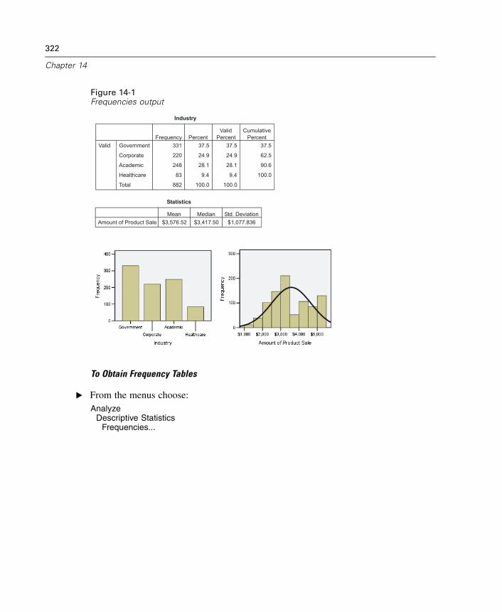
322

Chapter 14

Figure 14-1Frequencies output

Industry

331 37.5 37.5 37.5

220 24.9 24.9 62.5

248 28.1 28.1 90.6

83 9.4 9.4 100.0

882 100.0 100.0

Government

Corporate

Academic

Healthcare

Total

ValidFrequency Percent

ValidPercent

CumulativePercent

Statistics

$3,576.52 $3,417.50 $1,077.836Amount of Product SaleMean Median Std. Deviation

To Obtain Frequency Tables

E From the menus choose:Analyze

Descriptive StatisticsFrequencies...

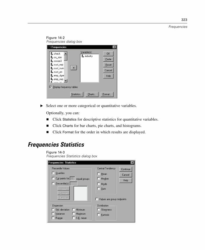
323

Frequencies

Figure 14-2Frequencies dialog box

E Select one or more categorical or quantitative variables.


Click Statistics for descriptive statistics for quantitative variables.

Click Charts for bar charts, pie charts, and histograms.

Click Format for the order in which results are displayed.

Frequencies StatisticsFigure 14-3Frequencies Statistics dialog box

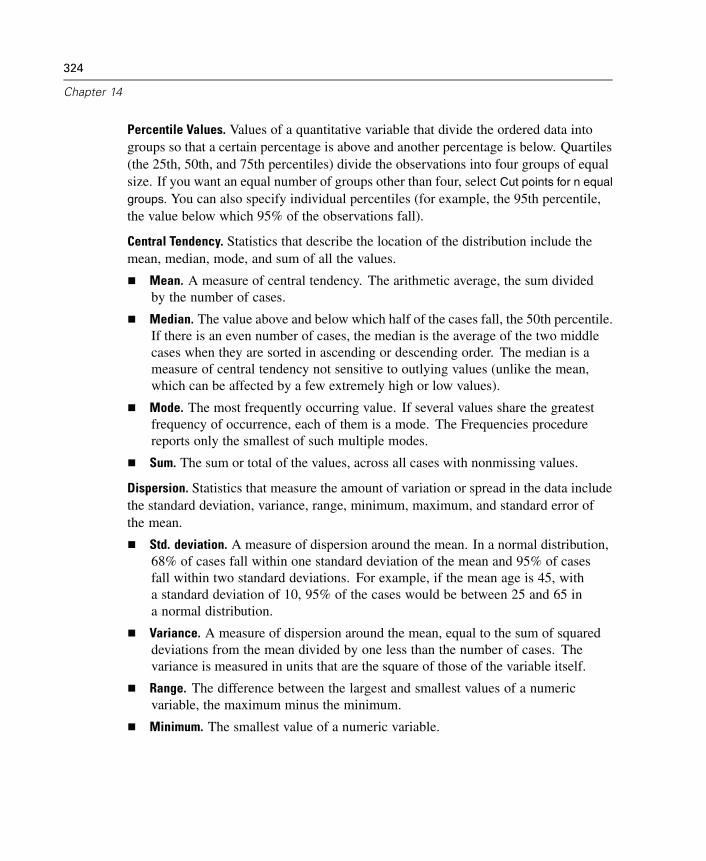
324

Chapter 14

Percentile Values. Values of a quantitative variable that divide the ordered data intogroups so that a certain percentage is above and another percentage is below. Quartiles(the 25th, 50th, and 75th percentiles) divide the observations into four groups of equalsize. If you want an equal number of groups other than four, select Cut points for n equal

groups. You can also specify individual percentiles (for example, the 95th percentile,the value below which 95% of the observations fall).

Central Tendency. Statistics that describe the location of the distribution include themean, median, mode, and sum of all the values.

Mean. A measure of central tendency. The arithmetic average, the sum dividedby the number of cases.

Median. The value above and below which half of the cases fall, the 50th percentile.If there is an even number of cases, the median is the average of the two middlecases when they are sorted in ascending or descending order. The median is ameasure of central tendency not sensitive to outlying values (unlike the mean,which can be affected by a few extremely high or low values).

Mode. The most frequently occurring value. If several values share the greatestfrequency of occurrence, each of them is a mode. The Frequencies procedurereports only the smallest of such multiple modes.

Sum. The sum or total of the values, across all cases with nonmissing values.

Dispersion. Statistics that measure the amount of variation or spread in the data includethe standard deviation, variance, range, minimum, maximum, and standard error ofthe mean.

Std. deviation. A measure of dispersion around the mean. In a normal distribution,68% of cases fall within one standard deviation of the mean and 95% of casesfall within two standard deviations. For example, if the mean age is 45, witha standard deviation of 10, 95% of the cases would be between 25 and 65 ina normal distribution.

Variance. A measure of dispersion around the mean, equal to the sum of squareddeviations from the mean divided by one less than the number of cases. Thevariance is measured in units that are the square of those of the variable itself.

Range. The difference between the largest and smallest values of a numericvariable, the maximum minus the minimum.

Minimum. The smallest value of a numeric variable.

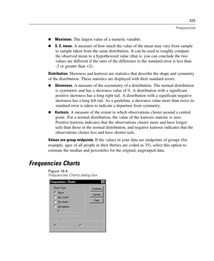
325

Frequencies

Maximum. The largest value of a numeric variable.

S. E. mean. A measure of how much the value of the mean may vary from sampleto sample taken from the same distribution. It can be used to roughly comparethe observed mean to a hypothesized value (that is, you can conclude the twovalues are different if the ratio of the difference to the standard error is less than-2 or greater than +2).

Distribution. Skewness and kurtosis are statistics that describe the shape and symmetryof the distribution. These statistics are displayed with their standard errors.

Skewness. A measure of the asymmetry of a distribution. The normal distributionis symmetric and has a skewness value of 0. A distribution with a significantpositive skewness has a long right tail. A distribution with a significant negativeskewness has a long left tail. As a guideline, a skewness value more than twice itsstandard error is taken to indicate a departure from symmetry.

Kurtosis. A measure of the extent to which observations cluster around a centralpoint. For a normal distribution, the value of the kurtosis statistic is zero.Positive kurtosis indicates that the observations cluster more and have longertails than those in the normal distribution, and negative kurtosis indicates that theobservations cluster less and have shorter tails.

Values are group midpoints. If the values in your data are midpoints of groups (forexample, ages of all people in their thirties are coded as 35), select this option toestimate the median and percentiles for the original, ungrouped data.

Frequencies ChartsFigure 14-4Frequencies Charts dialog box

326

Chapter 14

Chart Type. A pie chart displays the contribution of parts to a whole. Each slice of a piechart corresponds to a group that is defined by a single grouping variable. A bar chartdisplays the count for each distinct value or category as a separate bar, allowing youto compare categories visually. A histogram also has bars, but they are plotted alongan equal interval scale. The height of each bar is the count of values of a quantitativevariable falling within the interval. A histogram shows the shape, center, and spreadof the distribution. A normal curve superimposed on a histogram helps you judgewhether the data are normally distributed.

Chart Values. For bar charts, the scale axis can be labeled by frequency counts orpercentages.

Frequencies FormatFigure 14-5Frequencies Format dialog box

Order by. The frequency table can be arranged according to the actual values in the dataor according to the count (frequency of occurrence) of those values, and the tablecan be arranged in either ascending or descending order. However, if you request ahistogram or percentiles, Frequencies assumes that the variable is quantitative anddisplays its values in ascending order.

Multiple Variables. If you produce statistics tables for multiple variables, you can eitherdisplay all variables in a single table (Compare variables) or display a separate statisticstable for each variable (Organize output by variables).

Suppress tables with more than n categories. This option prevents the display of tableswith more than the specified number of values.

Chapter

15Descriptives

The Descriptives procedure displays univariate summary statistics for several variablesin a single table and calculates standardized values (z scores). Variables can be orderedby the size of their means (in ascending or descending order), alphabetically, or bythe order in which you select the variables (the default).

When z scores are saved, they are added to the data in the Data Editor and areavailable for charts, data listings, and analyses. When variables are recorded in differentunits (for example, gross domestic product per capita and percentage literate), a z-scoretransformation places variables on a common scale for easier visual comparison.

Example. If each case in your data contains the daily sales totals for each member ofthe sales staff (for example, one entry for Bob, one entry for Kim, one entry for Brian,etc.) collected each day for several months, the Descriptives procedure can computethe average daily sales for each staff member and can order the results from highestaverage sales to lowest average sales.

Statistics. Sample size, mean, minimum, maximum, standard deviation, variance,range, sum, standard error of the mean, and kurtosis and skewness with their standarderrors.

Data. Use numeric variables after you have screened them graphically for recordingerrors, outliers, and distributional anomalies. The Descriptives procedure is veryefficient for large files (thousands of cases).

Assumptions. Most of the available statistics (including z scores) are based onnormal theory and are appropriate for quantitative variables (interval- or ratio-levelmeasurements) with symmetric distributions. Avoid variables with unorderedcategories or skewed distributions. The distribution of z scores has the same shape asthat of the original data; therefore, calculating z scores is not a remedy for problem data.

327

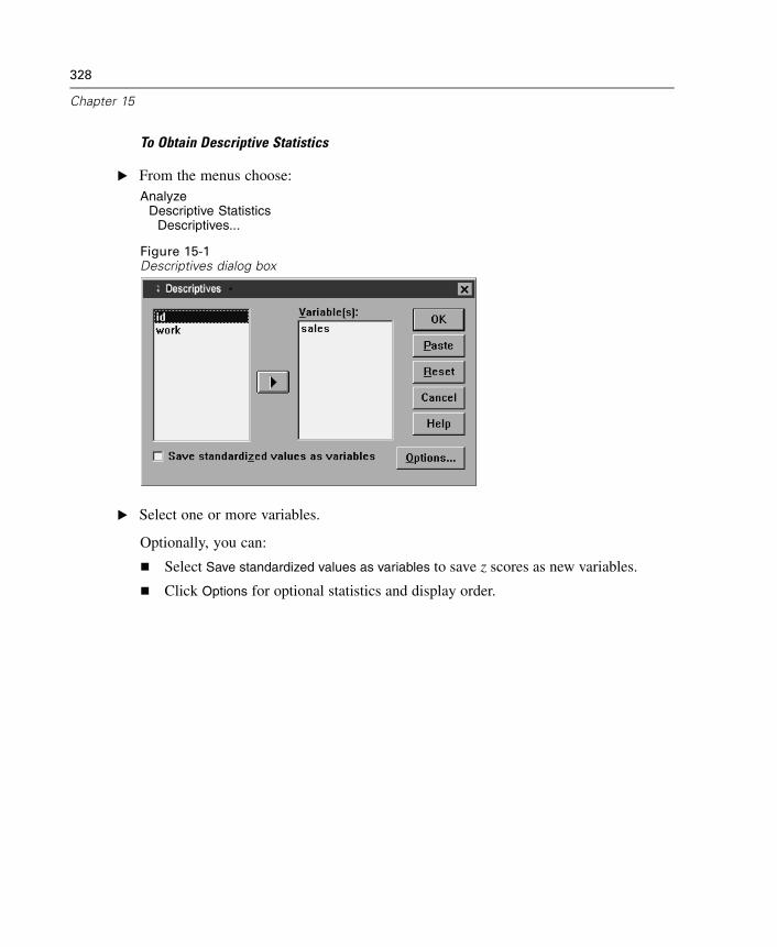
328

Chapter 15

To Obtain Descriptive Statistics


Descriptive StatisticsDescriptives...

Figure 15-1Descriptives dialog box

E Select one or more variables.


Select Save standardized values as variables to save z scores as new variables.

Click Options for optional statistics and display order.

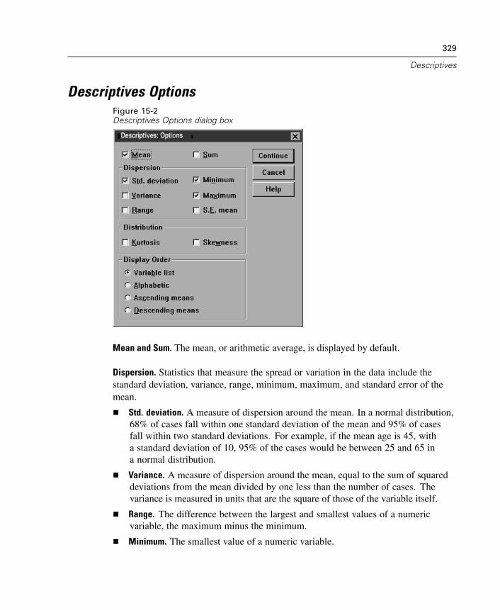
329

Descriptives

Descriptives OptionsFigure 15-2Descriptives Options dialog box

Mean and Sum. The mean, or arithmetic average, is displayed by default.

Dispersion. Statistics that measure the spread or variation in the data include thestandard deviation, variance, range, minimum, maximum, and standard error of themean.

Std. deviation. A measure of dispersion around the mean. In a normal distribution,68% of cases fall within one standard deviation of the mean and 95% of casesfall within two standard deviations. For example, if the mean age is 45, witha standard deviation of 10, 95% of the cases would be between 25 and 65 ina normal distribution.

Variance. A measure of dispersion around the mean, equal to the sum of squareddeviations from the mean divided by one less than the number of cases. Thevariance is measured in units that are the square of those of the variable itself.

Range. The difference between the largest and smallest values of a numericvariable, the maximum minus the minimum.


330

Chapter 15


S.E. mean. A measure of how much the value of the mean may vary from sampleto sample taken from the same distribution. It can be used to roughly comparethe observed mean to a hypothesized value (that is, you can conclude the twovalues are different if the ratio of the difference to the standard error is less than-2 or greater than +2).

Distribution. Kurtosis and skewness are statistics that characterize the shape andsymmetry of the distribution. These statistics are displayed with their standard errors.

Kurtosis. A measure of the extent to which observations cluster around a centralpoint. For a normal distribution, the value of the kurtosis statistic is zero.Positive kurtosis indicates that the observations cluster more and have longertails than those in the normal distribution, and negative kurtosis indicates that theobservations cluster less and have shorter tails.

Skewness. A measure of the asymmetry of a distribution. The normal distributionis symmetric and has a skewness value of 0. A distribution with a significantpositive skewness has a long right tail. A distribution with a significant negativeskewness has a long left tail. As a guideline, a skewness value more than twice itsstandard error is taken to indicate a departure from symmetry.

Display Order. By default, the variables are displayed in the order in which you selectedthem. Optionally, you can display variables alphabetically, by ascending means, or bydescending means.

DESCRIPTIVES Command Additional FeaturesThe SPSS command language also allows you to:

Save standardized scores (z scores) for some but not all variables (with theVARIABLES subcommand).

Specify names for new variables that contain standardized scores (with theVARIABLES subcommand).

Exclude from the analysis cases with missing values for any variable (with theMISSING subcommand).

Sort the variables in the display by the value of any statistic, not just the mean(with the SORT subcommand).


Chapter

16Explore

The Explore procedure produces summary statistics and graphical displays, either forall of your cases or separately for groups of cases. There are many reasons for usingthe Explore procedure—data screening, outlier identification, description, assumptionchecking, and characterizing differences among subpopulations (groups of cases).Data screening may show that you have unusual values, extreme values, gaps in thedata, or other peculiarities. Exploring the data can help to determine whether thestatistical techniques that you are considering for data analysis are appropriate. Theexploration may indicate that you need to transform the data if the technique requires anormal distribution. Or, you may decide that you need nonparametric tests.

Example. Look at the distribution of maze-learning times for rats under four differentreinforcement schedules. For each of the four groups, you can see if the distributionof times is approximately normal and whether the four variances are equal. You canalso identify the cases with the five largest and five smallest times. The boxplotsand stem-and-leaf plots graphically summarize the distribution of learning times foreach of the groups.

Statistics and plots. Mean, median, 5% trimmed mean, standard error, variance,standard deviation, minimum, maximum, range, interquartile range, skewness andkurtosis and their standard errors, confidence interval for the mean (and specifiedconfidence level), percentiles, Huber’s M-estimator, Andrews’ wave estimator,Hampel’s redescending M-estimator, Tukey’s biweight estimator, the five largest andfive smallest values, the Kolmogorov-Smirnov statistic with a Lilliefors significancelevel for testing normality, and the Shapiro-Wilk statistic. Boxplots, stem-and-leafplots, histograms, normality plots, and spread-versus-level plots with Levene testsand transformations.

Data. The Explore procedure can be used for quantitative variables (interval- orratio-level measurements). A factor variable (used to break the data into groups ofcases) should have a reasonable number of distinct values (categories). These values

331

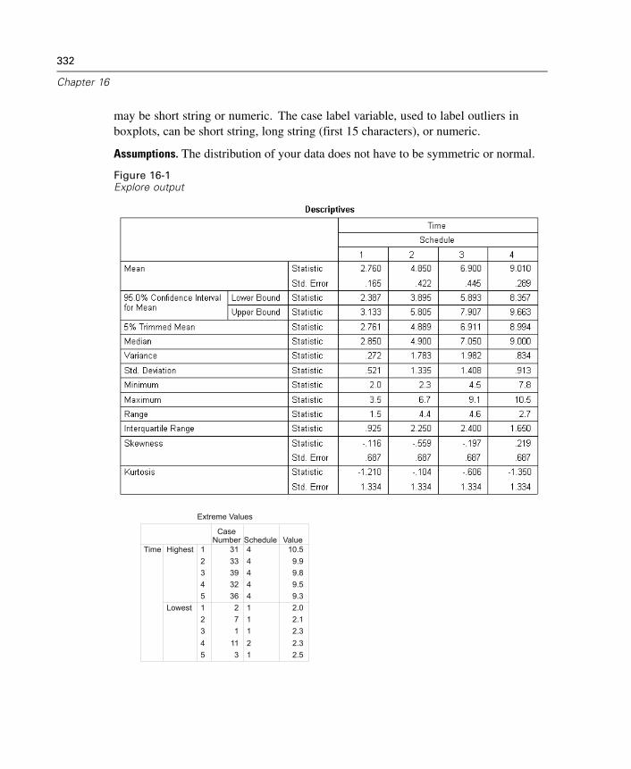
332

Chapter 16

may be short string or numeric. The case label variable, used to label outliers inboxplots, can be short string, long string (first 15 characters), or numeric.

Assumptions. The distribution of your data does not have to be symmetric or normal.

Figure 16-1Explore output

31 4 10.533 4 9.939 4 9.832 4 9.536 4 9.3

2 1 2.07 1 2.11 1 2.3

11 2 2.33 1 2.5

1234512345

Highest

Lowest

Time

CaseNumber Schedule Value

Extreme Values

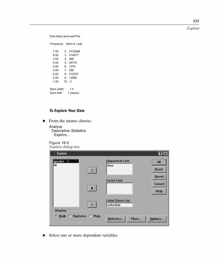
333

Explore

Time Stem-and-Leaf Plot

Frequency Stem & Leaf

7.00 2 . 0133589 6.00 3 . 014577 3.00 4 . 568 5.00 5 . 05779 4.00 6 . 1379 3.00 7 . 268 6.00 8 . 012237 5.00 9 . 13589 1.00 10 . 5

Stem width: 1.0 Each leaf: 1 case(s)

To Explore Your Data


Descriptive StatisticsExplore...

Figure 16-2Explore dialog box

E Select one or more dependent variables.

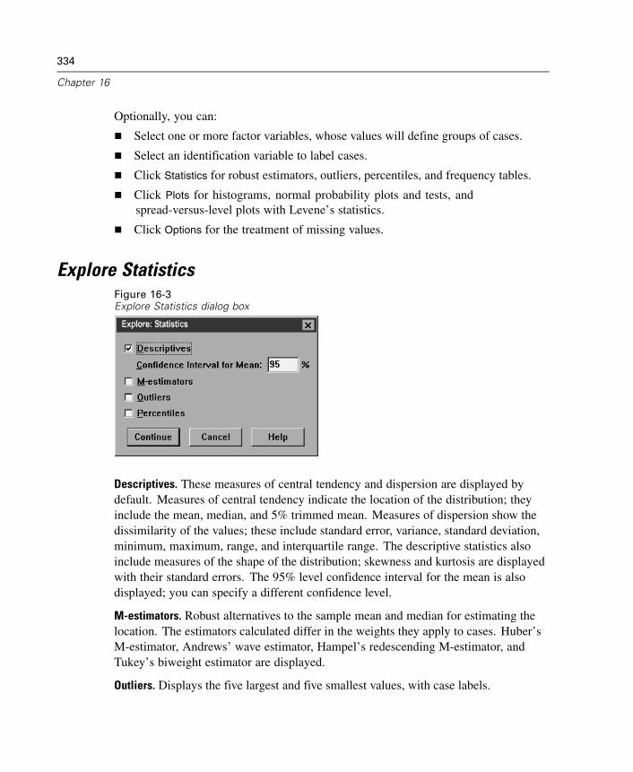
334

Chapter 16


Select one or more factor variables, whose values will define groups of cases.

Select an identification variable to label cases.

Click Statistics for robust estimators, outliers, percentiles, and frequency tables.

Click Plots for histograms, normal probability plots and tests, andspread-versus-level plots with Levene’s statistics.

Click Options for the treatment of missing values.

Explore StatisticsFigure 16-3Explore Statistics dialog box

Descriptives. These measures of central tendency and dispersion are displayed bydefault. Measures of central tendency indicate the location of the distribution; theyinclude the mean, median, and 5% trimmed mean. Measures of dispersion show thedissimilarity of the values; these include standard error, variance, standard deviation,minimum, maximum, range, and interquartile range. The descriptive statistics alsoinclude measures of the shape of the distribution; skewness and kurtosis are displayedwith their standard errors. The 95% level confidence interval for the mean is alsodisplayed; you can specify a different confidence level.

M-estimators. Robust alternatives to the sample mean and median for estimating thelocation. The estimators calculated differ in the weights they apply to cases. Huber’sM-estimator, Andrews’ wave estimator, Hampel’s redescending M-estimator, andTukey’s biweight estimator are displayed.

Outliers. Displays the five largest and five smallest values, with case labels.

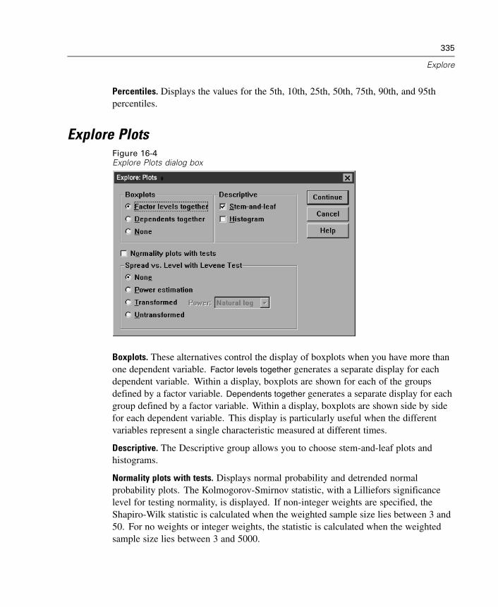
335

Explore

Percentiles. Displays the values for the 5th, 10th, 25th, 50th, 75th, 90th, and 95thpercentiles.

Explore PlotsFigure 16-4Explore Plots dialog box

Boxplots. These alternatives control the display of boxplots when you have more thanone dependent variable. Factor levels together generates a separate display for eachdependent variable. Within a display, boxplots are shown for each of the groupsdefined by a factor variable. Dependents together generates a separate display for eachgroup defined by a factor variable. Within a display, boxplots are shown side by sidefor each dependent variable. This display is particularly useful when the differentvariables represent a single characteristic measured at different times.

Descriptive. The Descriptive group allows you to choose stem-and-leaf plots andhistograms.

Normality plots with tests. Displays normal probability and detrended normalprobability plots. The Kolmogorov-Smirnov statistic, with a Lilliefors significancelevel for testing normality, is displayed. If non-integer weights are specified, theShapiro-Wilk statistic is calculated when the weighted sample size lies between 3 and50. For no weights or integer weights, the statistic is calculated when the weightedsample size lies between 3 and 5000.

336

Chapter 16

Spread vs. Level with Levene Test. Controls data transformation for spread-versus-levelplots. For all spread-versus-level plots, the slope of the regression line and Levene’srobust tests for homogeneity of variance are displayed. If you select a transformation,Levene’s tests are based on the transformed data. If no factor variable is selected,spread-versus-level plots are not produced. Power estimation produces a plot ofthe natural logs of the interquartile ranges against the natural logs of the mediansfor all cells, as well as an estimate of the power transformation for achievingequal variances in the cells. A spread-versus-level plot helps to determine thepower for a transformation to stabilize (make more equal) variances across groups.Transformed allows you to select one of the power alternatives, perhaps following therecommendation from power estimation, and produces plots of transformed data. Theinterquartile range and median of the transformed data are plotted. Untransformed

produces plots of the raw data. This is equivalent to a transformation with a power of 1.

Explore Power Transformations

These are the power transformations for spread-versus-level plots. To transform data,you must select a power for the transformation. You can choose one of the followingalternatives:

Natural log. Natural log transformation. This is the default.

1/square root. For each data value, the reciprocal of the square root is calculated.

Reciprocal. The reciprocal of each data value is calculated.

Square root. The square root of each data value is calculated.

Square. Each data value is squared.

Cube. Each data value is cubed.

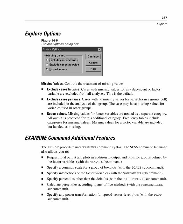
337

Explore

Explore OptionsFigure 16-5Explore Options dialog box

Missing Values. Controls the treatment of missing values.

Exclude cases listwise. Cases with missing values for any dependent or factorvariable are excluded from all analyses. This is the default.

Exclude cases pairwise. Cases with no missing values for variables in a group (cell)are included in the analysis of that group. The case may have missing values forvariables used in other groups.

Report values. Missing values for factor variables are treated as a separate category.All output is produced for this additional category. Frequency tables includecategories for missing values. Missing values for a factor variable are includedbut labeled as missing.

EXAMINE Command Additional Features

The Explore procedure uses EXAMINE command syntax. The SPSS command languagealso allows you to:

Request total output and plots in addition to output and plots for groups defined bythe factor variables (with the TOTAL subcommand).

Specify a common scale for a group of boxplots (with the SCALE subcommand).

Specify interactions of the factor variables (with the VARIABLES subcommand).

Specify percentiles other than the defaults (with the PERCENTILES subcommand).

Calculate percentiles according to any of five methods (with the PERCENTILESsubcommand).

Specify any power transformation for spread-versus-level plots (with the PLOTsubcommand).

338

Chapter 16

Specify the number of extreme values to be displayed (with the STATISTICSsubcommand).

Specify parameters for the M-estimators, robust estimators of location (with theMESTIMATORS subcommand).


Chapter

17Crosstabs

The Crosstabs procedure forms two-way and multiway tables and provides a variety oftests and measures of association for two-way tables. The structure of the table andwhether categories are ordered determine what test or measure to use.

Crosstabs’ statistics and measures of association are computed for two-way tablesonly. If you specify a row, a column, and a layer factor (control variable), the Crosstabsprocedure forms one panel of associated statistics and measures for each value ofthe layer factor (or a combination of values for two or more control variables). Forexample, if gender is a layer factor for a table of married (yes, no) against life (is lifeexciting, routine, or dull), the results for a two-way table for the females are computedseparately from those for the males and printed as panels following one another.

Example. Are customers from small companies more likely to be profitable in salesof services (for example, training and consulting) than those from larger companies?From a crosstabulation, you might learn that the majority of small companies (fewerthan 500 employees) yield high service profits, while the majority of large companies(more than 2,500 employees) yield low service profits.

Statistics and measures of association. Pearson chi-square, likelihood-ratio chi-square,linear-by-linear association test, Fisher’s exact test, Yates’ corrected chi-square,Pearson’s r, Spearman’s rho, contingency coefficient, phi, Cramér’s V, symmetric andasymmetric lambdas, Goodman and Kruskal’s tau, uncertainty coefficient, gamma,Somers’ d, Kendall’s tau-b, Kendall’s tau-c, eta coefficient, Cohen’s kappa, relativerisk estimate, odds ratio, McNemar test, and Cochran’s and Mantel-Haenszel statistics.

Data. To define the categories of each table variable, use values of a numeric or shortstring (eight or fewer characters) variable. For example, for gender, you could code thedata as 1 and 2 or as male and female.

Assumptions. Some statistics and measures assume ordered categories (ordinal data)or quantitative values (interval or ratio data), as discussed in the section on statistics.Others are valid when the table variables have unordered categories (nominal data).

339

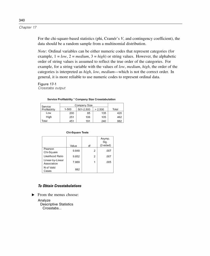
340

Chapter 17

For the chi-square-based statistics (phi, Cramér’s V, and contingency coefficient), thedata should be a random sample from a multinomial distribution.

Note: Ordinal variables can be either numeric codes that represent categories (forexample, 1 = low, 2 = medium, 3 = high) or string values. However, the alphabeticorder of string values is assumed to reflect the true order of the categories. Forexample, for a string variable with the values of low, medium, high, the order of thecategories is interpreted as high, low, medium—which is not the correct order. Ingeneral, it is more reliable to use numeric codes to represent ordinal data.

Figure 17-1Crosstabs output

To Obtain Crosstabulations


Descriptive StatisticsCrosstabs...

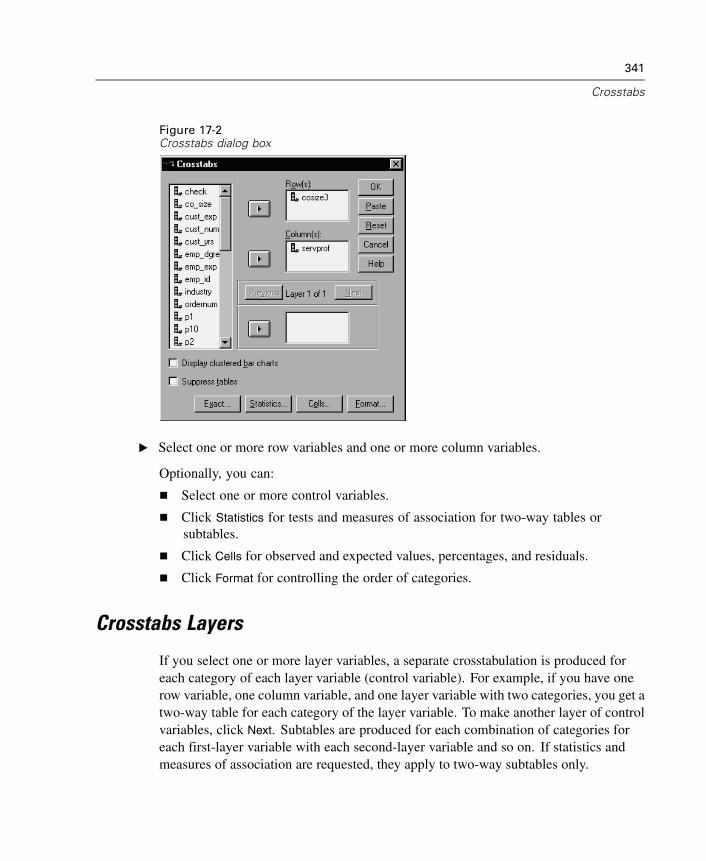
341

Crosstabs

Figure 17-2Crosstabs dialog box

E Select one or more row variables and one or more column variables.


Select one or more control variables.

Click Statistics for tests and measures of association for two-way tables orsubtables.

Click Cells for observed and expected values, percentages, and residuals.

Click Format for controlling the order of categories.

Crosstabs Layers

If you select one or more layer variables, a separate crosstabulation is produced foreach category of each layer variable (control variable). For example, if you have onerow variable, one column variable, and one layer variable with two categories, you get atwo-way table for each category of the layer variable. To make another layer of controlvariables, click Next. Subtables are produced for each combination of categories foreach first-layer variable with each second-layer variable and so on. If statistics andmeasures of association are requested, they apply to two-way subtables only.

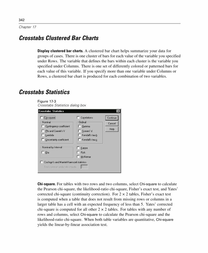
342

Chapter 17

Crosstabs Clustered Bar Charts

Display clustered bar charts. A clustered bar chart helps summarize your data forgroups of cases. There is one cluster of bars for each value of the variable you specifiedunder Rows. The variable that defines the bars within each cluster is the variable youspecified under Columns. There is one set of differently colored or patterned bars foreach value of this variable. If you specify more than one variable under Columns orRows, a clustered bar chart is produced for each combination of two variables.

Crosstabs StatisticsFigure 17-3Crosstabs Statistics dialog box

Chi-square. For tables with two rows and two columns, select Chi-square to calculatethe Pearson chi-square, the likelihood-ratio chi-square, Fisher’s exact test, and Yates’corrected chi-square (continuity correction). For 2 × 2 tables, Fisher’s exact testis computed when a table that does not result from missing rows or columns in alarger table has a cell with an expected frequency of less than 5. Yates’ correctedchi-square is computed for all other 2 × 2 tables. For tables with any number ofrows and columns, select Chi-square to calculate the Pearson chi-square and thelikelihood-ratio chi-square. When both table variables are quantitative, Chi-square

yields the linear-by-linear association test.

343

Crosstabs

Correlations. For tables in which both rows and columns contain ordered values,Correlations yields Spearman’s correlation coefficient, rho (numeric data only).Spearman’s rho is a measure of association between rank orders. When both tablevariables (factors) are quantitative, Correlations yields the Pearson correlationcoefficient, r, a measure of linear association between the variables.

Nominal. For nominal data (no intrinsic order, such as Catholic, Protestant, andJewish), you can select Phi (coefficient) and Cramér’s V, Contingency coefficient,Lambda (symmetric and asymmetric lambdas and Goodman and Kruskal’s tau), andUncertainty coefficient.

Contingency coefficient. A measure of association based on chi-square. The valueranges between 0 and 1, with 0 indicating no association between the row andcolumn variables and values close to 1 indicating a high degree of associationbetween the variables. The maximum value possible depends on the number ofrows and columns in a table.

Phi and Cramer's V. Phi is a chi-square-based measure of association that involvesdividing the chi-square statistic by the sample size and taking the square root ofthe result. Cramer's V is a measure of association based on chi-square.

Lambda. A measure of association that reflects the proportional reduction in errorwhen values of the independent variable are used to predict values of the dependentvariable. A value of 1 means that the independent variable perfectly predicts thedependent variable. A value of 0 means that the independent variable is no helpin predicting the dependent variable.

Uncertainty coefficient. A measure of association that indicates the proportionalreduction in error when values of one variable are used to predict values of the othervariable. For example, a value of 0.83 indicates that knowledge of one variablereduces error in predicting values of the other variable by 83%. The programcalculates both symmetric and asymmetric versions of the uncertainty coefficient.

Ordinal. For tables in which both rows and columns contain ordered values, selectGamma (zero-order for 2-way tables and conditional for 3-way to 10-way tables),Kendall’s tau-b, and Kendall’s tau-c. For predicting column categories from rowcategories, select Somers’ d.

Gamma. A symmetric measure of association between two ordinal variables thatranges between -1 and 1. Values close to an absolute value of 1 indicate a strongrelationship between the two variables. Values close to 0 indicate little or no

344

Chapter 17

relationship. For 2-way tables, zero-order gammas are displayed. For 3-way ton-way tables, conditional gammas are displayed.

Somers' d. A measure of association between two ordinal variables that rangesfrom -1 to 1. Values close to an absolute value of 1 indicate a strong relationshipbetween the two variables, and values close to 0 indicate little or no relationshipbetween the variables. Somers' d is an asymmetric extension of gamma that differsonly in the inclusion of the number of pairs not tied on the independent variable. Asymmetric version of this statistic is also calculated.

Kendall's tau-b. A nonparametric measure of correlation for ordinal or rankedvariables that take ties into account. The sign of the coefficient indicates thedirection of the relationship, and its absolute value indicates the strength, withlarger absolute values indicating stronger relationships. Possible values range from-1 to 1, but a value of -1 or +1 can be obtained only from square tables.

Kendall's tau-c. A nonparametric measure of association for ordinal variables thatignores ties. The sign of the coefficient indicates the direction of the relationship,and its absolute value indicates the strength, with larger absolute values indicatingstronger relationships. Possible values range from -1 to 1, but a value of -1 or +1can be obtained only from square tables.

Nominal by Interval. When one variable is categorical and the other is quantitative,select Eta. The categorical variable must be coded numerically.

Eta. A measure of association that ranges from 0 to 1, with 0 indicating noassociation between the row and column variables and values close to 1 indicatinga high degree of association. Eta is appropriate for a dependent variable measuredon an interval scale (for example, income) and an independent variable with alimited number of categories (for example, gender). Two eta values are computed:one treats the row variable as the interval variable, and the other treats the columnvariable as the interval variable.

Kappa. Cohen's kappa measures the agreement between the evaluations of two raterswhen both are rating the same object. A value of 1 indicates perfect agreement. Avalue of 0 indicates that agreement is no better than chance. Kappa is available onlyfor tables in which both variables use the same category values and both variables havethe same number of categories.

Risk. For 2 x 2 tables, a measure of the strength of the association between the presenceof a factor and the occurrence of an event. If the confidence interval for the statisticincludes a value of 1, you cannot assume that the factor is associated with the event.

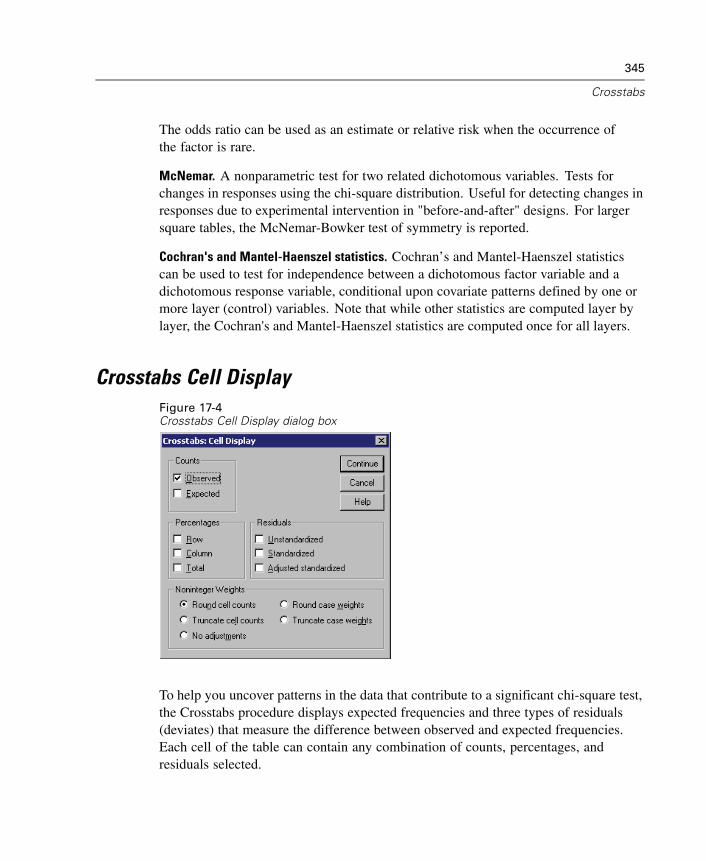
345

Crosstabs

The odds ratio can be used as an estimate or relative risk when the occurrence ofthe factor is rare.

McNemar. A nonparametric test for two related dichotomous variables. Tests forchanges in responses using the chi-square distribution. Useful for detecting changes inresponses due to experimental intervention in "before-and-after" designs. For largersquare tables, the McNemar-Bowker test of symmetry is reported.

Cochran's and Mantel-Haenszel statistics. Cochran’s and Mantel-Haenszel statisticscan be used to test for independence between a dichotomous factor variable and adichotomous response variable, conditional upon covariate patterns defined by one ormore layer (control) variables. Note that while other statistics are computed layer bylayer, the Cochran's and Mantel-Haenszel statistics are computed once for all layers.

Crosstabs Cell DisplayFigure 17-4Crosstabs Cell Display dialog box

To help you uncover patterns in the data that contribute to a significant chi-square test,the Crosstabs procedure displays expected frequencies and three types of residuals(deviates) that measure the difference between observed and expected frequencies.Each cell of the table can contain any combination of counts, percentages, andresiduals selected.

346

Chapter 17

Counts. The number of cases actually observed and the number of cases expected if therow and column variables are independent of each other.

Percentages. The percentages can add up across the rows or down the columns. Thepercentages of the total number of cases represented in the table (one layer) are alsoavailable.

Residuals. Raw unstandardized residuals give the difference between the observed andexpected values. Standardized and adjusted standardized residuals are also available.

Unstandardized. The difference between an observed value and the expected value.The expected value is the number of cases you would expect in the cell if therewere no relationship between the two variables. A positive residual indicatesthat there are more cases in the cell than there would be if the row and columnvariables were independent.

Standardized. The residual divided by an estimate of its standard deviation.Standardized residuals, which are also known as Pearson residuals, have a mean of0 and a standard deviation of 1.

Adjusted standardized. The residual for a cell (observed minus expected value)divided by an estimate of its standard error. The resulting standardized residual isexpressed in standard deviation units above or below the mean.

Noninteger Weights. Cell counts are normally integer values, since they represent thenumber of cases in each cell. But if the data file is currently weighted by a weightvariable with fractional values (for example, 1.25), cell counts can also be fractionalvalues. You can truncate or round either before or after calculating the cell counts oruse fractional cell counts for both table display and statistical calculations.

Round cell counts. Case weights are used as is but the accumulated weights in thecells are rounded before computing any statistics.

Truncate cell counts. Case weights are used as is but the accumulated weights in thecells are truncated before computing any statistics.

Round case weights. Case weights are rounded before use.

Truncate case weights. Case weights are truncated before use.

No adjustments. Case weights are used as is and fractional cell counts are used.However, when Exact Statistics (available only with the Exact Tests option) arerequested, the accumulated weights in the cells are either truncated or roundedbefore computing the Exact test statistics.

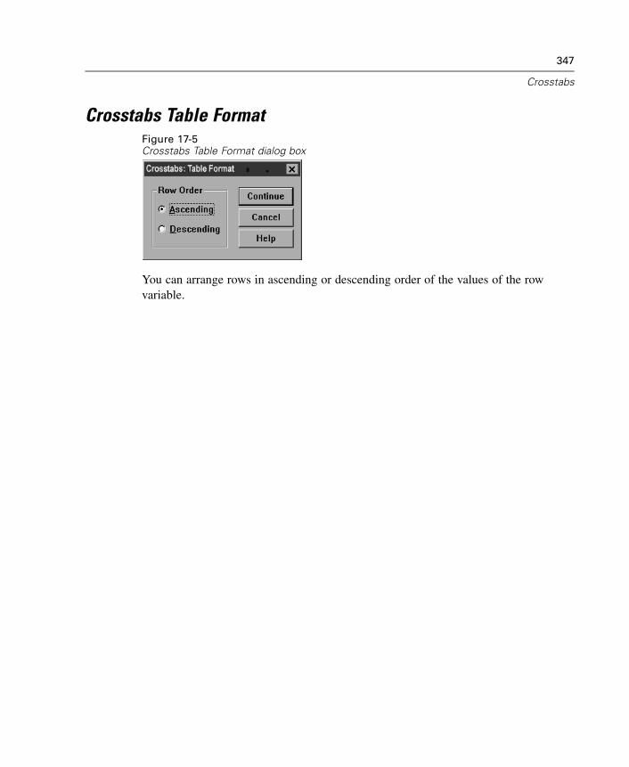
347

Crosstabs

Crosstabs Table FormatFigure 17-5Crosstabs Table Format dialog box

You can arrange rows in ascending or descending order of the values of the rowvariable.

Chapter

18Summarize

The Summarize procedure calculates subgroup statistics for variables withincategories of one or more grouping variables. All levels of the grouping variableare crosstabulated. You can choose the order in which the statistics are displayed.Summary statistics for each variable across all categories are also displayed. Datavalues in each category can be listed or suppressed. With large datasets, you canchoose to list only the first n cases.

Example. What is the average product sales amount by region and customer industry?You might discover that the average sales amount is slightly higher in the westernregion than in other regions, with corporate customers in the western region yieldingthe highest average sales amount.

Statistics. Sum, number of cases, mean, median, grouped median, standard error ofthe mean, minimum, maximum, range, variable value of the first category of thegrouping variable, variable value of the last category of the grouping variable, standarddeviation, variance, kurtosis, standard error of kurtosis, skewness, standard errorof skewness, percentage of total sum, percentage of total N, percentage of sum in,percentage of N in, geometric mean, and harmonic mean.

Data. Grouping variables are categorical variables whose values can be numeric orshort string. The number of categories should be reasonably small. The other variablesshould be able to be ranked.

Assumptions. Some of the optional subgroup statistics, such as the mean and standarddeviation, are based on normal theory and are appropriate for quantitative variableswith symmetric distributions. Robust statistics, such as the median and the range,are appropriate for quantitative variables that may or may not meet the assumptionof normality.

349

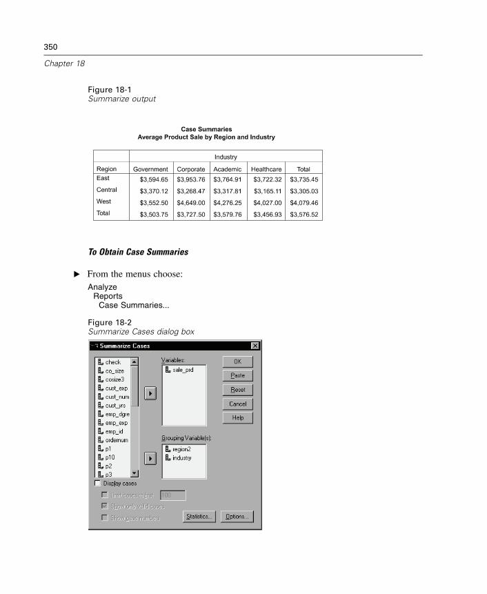
350

Chapter 18

Figure 18-1Summarize output

To Obtain Case Summaries


ReportsCase Summaries...

Figure 18-2Summarize Cases dialog box

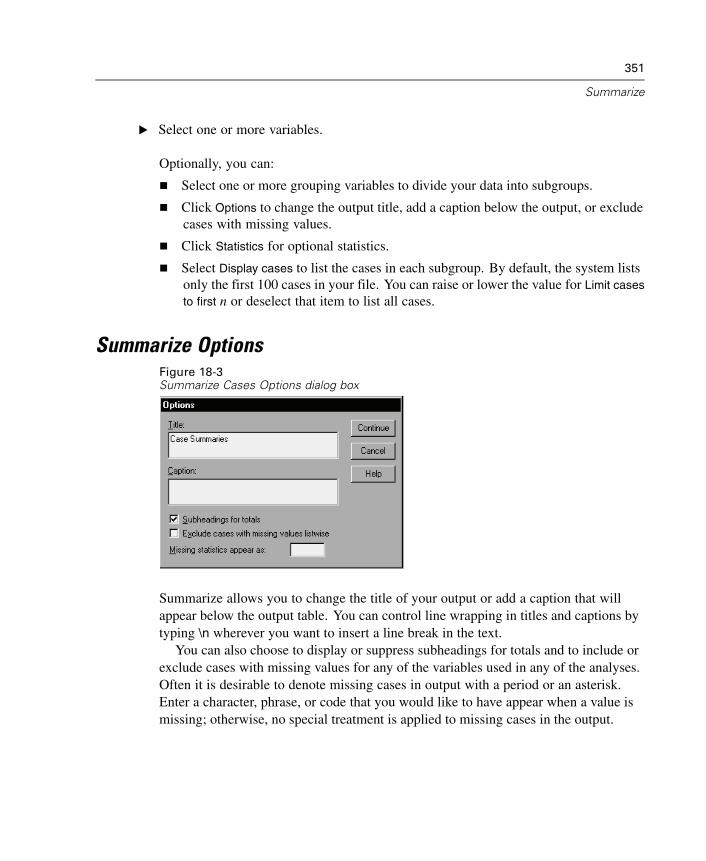
351

Summarize

E Select one or more variables.


Select one or more grouping variables to divide your data into subgroups.

Click Options to change the output title, add a caption below the output, or excludecases with missing values.

Click Statistics for optional statistics.

Select Display cases to list the cases in each subgroup. By default, the system listsonly the first 100 cases in your file. You can raise or lower the value for Limit casesto first n or deselect that item to list all cases.

Summarize OptionsFigure 18-3Summarize Cases Options dialog box

Summarize allows you to change the title of your output or add a caption that willappear below the output table. You can control line wrapping in titles and captions bytyping \n wherever you want to insert a line break in the text.

You can also choose to display or suppress subheadings for totals and to include orexclude cases with missing values for any of the variables used in any of the analyses.Often it is desirable to denote missing cases in output with a period or an asterisk.Enter a character, phrase, or code that you would like to have appear when a value ismissing; otherwise, no special treatment is applied to missing cases in the output.

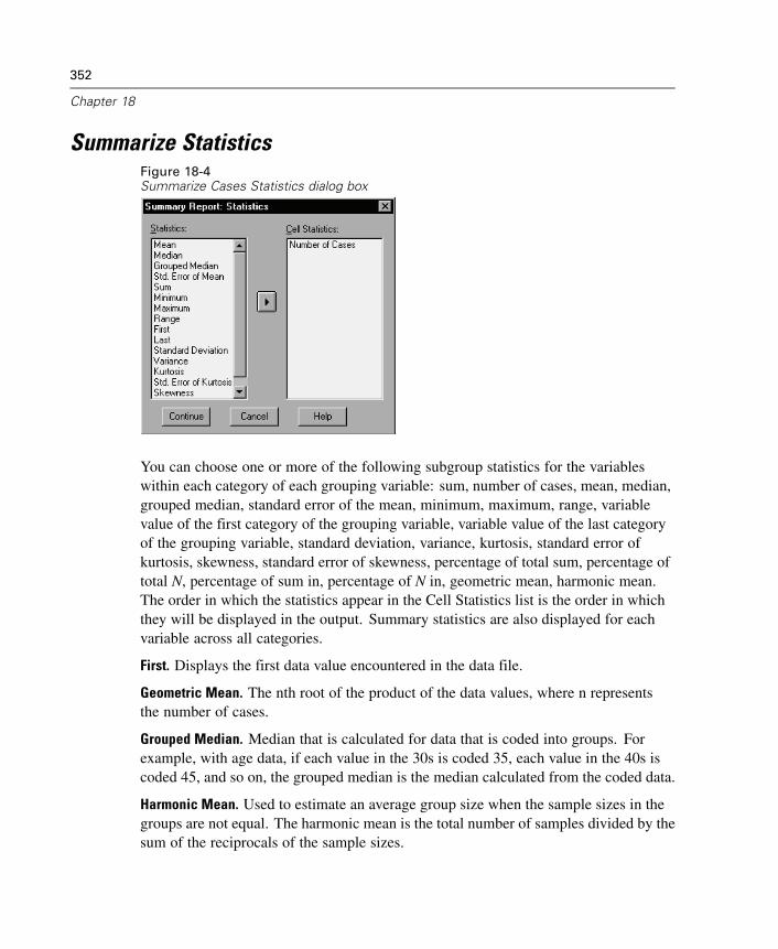
352

Chapter 18

Summarize StatisticsFigure 18-4Summarize Cases Statistics dialog box

You can choose one or more of the following subgroup statistics for the variableswithin each category of each grouping variable: sum, number of cases, mean, median,grouped median, standard error of the mean, minimum, maximum, range, variablevalue of the first category of the grouping variable, variable value of the last categoryof the grouping variable, standard deviation, variance, kurtosis, standard error ofkurtosis, skewness, standard error of skewness, percentage of total sum, percentage oftotal N, percentage of sum in, percentage of N in, geometric mean, harmonic mean.The order in which the statistics appear in the Cell Statistics list is the order in whichthey will be displayed in the output. Summary statistics are also displayed for eachvariable across all categories.

First. Displays the first data value encountered in the data file.

Geometric Mean. The nth root of the product of the data values, where n representsthe number of cases.

Grouped Median. Median that is calculated for data that is coded into groups. Forexample, with age data, if each value in the 30s is coded 35, each value in the 40s iscoded 45, and so on, the grouped median is the median calculated from the coded data.

Harmonic Mean. Used to estimate an average group size when the sample sizes in thegroups are not equal. The harmonic mean is the total number of samples divided by thesum of the reciprocals of the sample sizes.

353

Summarize

Kurtosis. A measure of the extent to which observations cluster around a central point.For a normal distribution, the value of the kurtosis statistic is zero. Positive kurtosisindicates that the observations cluster more and have longer tails than those in thenormal distribution, and negative kurtosis indicates that the observations cluster lessand have shorter tails.

Last. Displays the last data value encountered in the data file.


Mean. A measure of central tendency. The arithmetic average, the sum divided bythe number of cases.

Median. The value above and below which half of the cases fall, the 50th percentile. Ifthere is an even number of cases, the median is the average of the two middle caseswhen they are sorted in ascending or descending order. The median is a measureof central tendency not sensitive to outlying values (unlike the mean, which can beaffected by a few extremely high or low values).


N. The number of cases (observations or records).

Percent of Total N. Percentage of the total number of cases in each category.

Percent of Total Sum. Percentage of the total sum in each category.

Range. The difference between the largest and smallest values of a numeric variable,the maximum minus the minimum.

Skewness. A measure of the asymmetry of a distribution. The normal distribution issymmetric and has a skewness value of 0. A distribution with a significant positiveskewness has a long right tail. A distribution with a significant negative skewness has along left tail. As a guideline, a skewness value more than twice its standard error istaken to indicate a departure from symmetry.

Standard Error of Kurtosis. The ratio of kurtosis to its standard error can be used as atest of normality (that is, you can reject normality if the ratio is less than -2 or greaterthan +2). A large positive value for kurtosis indicates that the tails of the distributionare longer than those of a normal distribution; a negative value for kurtosis indicatesshorter tails (becoming like those of a box-shaped uniform distribution).

354

Chapter 18

Standard Error of Skewness. The ratio of skewness to its standard error can be used as atest of normality (that is, you can reject normality if the ratio is less than -2 or greaterthan +2). A large positive value for skewness indicates a long right tail; an extremenegative value indicates a long left tail.


Variance. A measure of dispersion around the mean, equal to the sum of squareddeviations from the mean divided by one less than the number of cases. The variance ismeasured in units that are the square of those of the variable itself.

Chapter

19Means

The Means procedure calculates subgroup means and related univariate statisticsfor dependent variables within categories of one or more independent variables.Optionally, you can obtain a one-way analysis of variance, eta, and tests for linearity.

Example. Measure the average amount of fat absorbed by three different types ofcooking oil, and perform a one-way analysis of variance to see whether the meansdiffer.

Statistics. Sum, number of cases, mean, median, grouped median, standard error ofthe mean, minimum, maximum, range, variable value of the first category of thegrouping variable, variable value of the last category of the grouping variable, standarddeviation, variance, kurtosis, standard error of kurtosis, skewness, standard errorof skewness, percentage of total sum, percentage of total N, percentage of sum in,percentage of N in, geometric mean, and harmonic mean. Options include analysis ofvariance, eta, eta squared, and tests for linearity R and R2.

Data. The dependent variables are quantitative, and the independent variables arecategorical. The values of categorical variables can be numeric or short string.

Assumptions. Some of the optional subgroup statistics, such as the mean and standarddeviation, are based on normal theory and are appropriate for quantitative variableswith symmetric distributions. Robust statistics, such as the median, are appropriate forquantitative variables that may or may not meet the assumption of normality. Analysisof variance is robust to departures from normality, but the data in each cell should besymmetric. Analysis of variance also assumes that the groups come from populationswith equal variances. To test this assumption, use Levene’s homogeneity-of-variancetest, available in the One-Way ANOVA procedure.

355

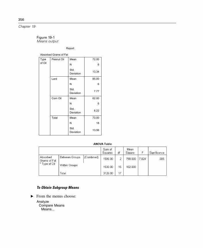
356

Chapter 19

Figure 19-1Means output

Absorbed Grams of Fat

72.00

6

13.34

85.00

6

7.77

62.00

6

8.22

73.00

18

13.56

Mean

N

Std.Deviation

Mean

N

Std.Deviation

Mean

N

Std.Deviation

Mean

N

Std.Deviation

Peanut Oil

Lard

Corn Oil

Total

Typeof Oil

Report

To Obtain Subgroup Means


Compare MeansMeans...

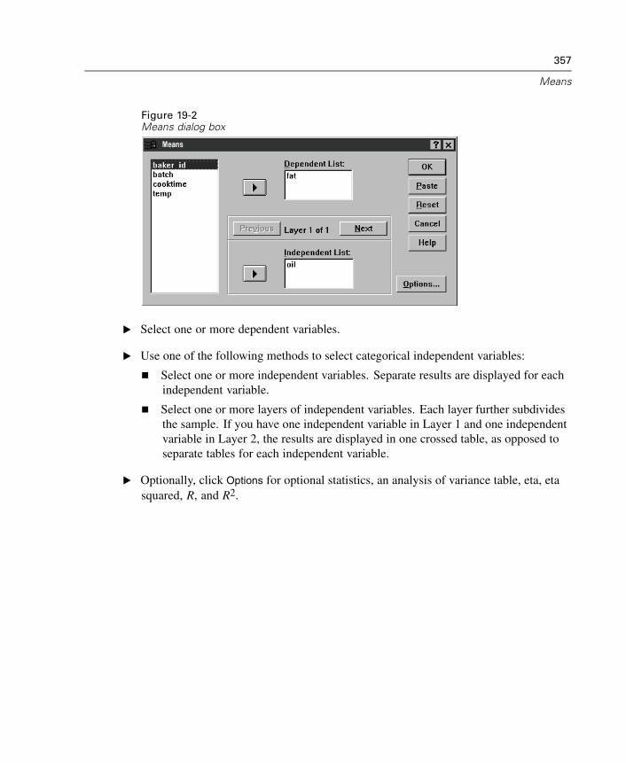
357

Means

Figure 19-2Means dialog box


E Use one of the following methods to select categorical independent variables:

Select one or more independent variables. Separate results are displayed for eachindependent variable.

Select one or more layers of independent variables. Each layer further subdividesthe sample. If you have one independent variable in Layer 1 and one independentvariable in Layer 2, the results are displayed in one crossed table, as opposed toseparate tables for each independent variable.

E Optionally, click Options for optional statistics, an analysis of variance table, eta, etasquared, R, and R2.

358

Chapter 19

Means OptionsFigure 19-3Means Options dialog box

You can choose one or more of the following subgroup statistics for the variableswithin each category of each grouping variable: sum, number of cases, mean, median,grouped median, standard error of the mean, minimum, maximum, range, variablevalue of the first category of the grouping variable, variable value of the last category ofthe grouping variable, standard deviation, variance, kurtosis, standard error of kurtosis,skewness, standard error of skewness, percentage of total sum, percentage of total N,percentage of sum in, percentage of N in, geometric mean, and harmonic mean. Youcan change the order in which the subgroup statistics appear. The order in which thestatistics appear in the Cell Statistics list is the order in which they are displayed in theoutput. Summary statistics are also displayed for each variable across all categories.



359

Means










Percent of total N. Percentage of the total number of cases in each category.

Percent of total sum. Percentage of the total sum in each category.


Skewness. A measure of the asymmetry of a distribution. The normal distribution issymmetric and has a skewness value of 0. A distribution with a significant positiveskewness has a long right tail. A distribution with a significant negative skewness has along left tail. As a guideline, a skewness value more than twice its standard error istaken to indicate a departure from symmetry.

360

Chapter 19





Statistics for First Layer

Anova table and eta. Displays a one-way analysis-of-variance table and calculates etaand eta squared (measures of association) for each independent variable in the firstlayer.

Test for linearity. Calculates the sum of squares, degrees of freedom, and mean squareassociated with linear and nonlinear components, as well as the F ratio, R and Rsquared. Linearity is not calculated if the independent variable is a short string.

Chapter

20OLAP Cubes

The OLAP (Online Analytical Processing) Cubes procedure calculates totals, means,and other univariate statistics for continuous summary variables within categories ofone or more categorical grouping variables. A separate layer in the table is created foreach category of each grouping variable.

Example. Total and average sales for different regions and product lines within regions.

Statistics. Sum, number of cases, mean, median, grouped median, standard error ofthe mean, minimum, maximum, range, variable value of the first category of thegrouping variable, variable value of the last category of the grouping variable, standarddeviation, variance, kurtosis, standard error of kurtosis, skewness, standard error ofskewness, percentage of total cases, percentage of total sum, percentage of totalcases within grouping variables, percentage of total sum within grouping variables,geometric mean, and harmonic mean.

Data. The summary variables are quantitative (continuous variables measured on aninterval or ratio scale), and the grouping variables are categorical. The values ofcategorical variables can be numeric or short string.

Assumptions. Some of the optional subgroup statistics, such as the mean and standarddeviation, are based on normal theory and are appropriate for quantitative variableswith symmetric distributions. Robust statistics, such as the median and range, areappropriate for quantitative variables that may or may not meet the assumption ofnormality.

361

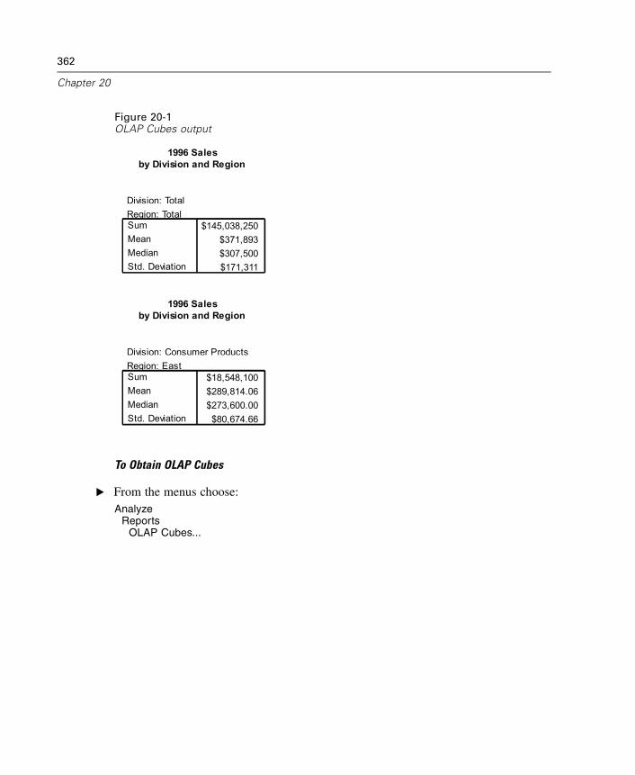
362

Chapter 20

Figure 20-1OLAP Cubes output

Division: TotalRegion: Total

$145,038,250$371,893$307,500$171,311

SumMeanMedianStd. Deviation

1996 Salesby Division and Region

Division: Consumer ProductsRegion: East

$18,548,100$289,814.06$273,600.00$80,674.66

SumMeanMedianStd. Deviation

1996 Salesby Division and Region

To Obtain OLAP Cubes


ReportsOLAP Cubes...

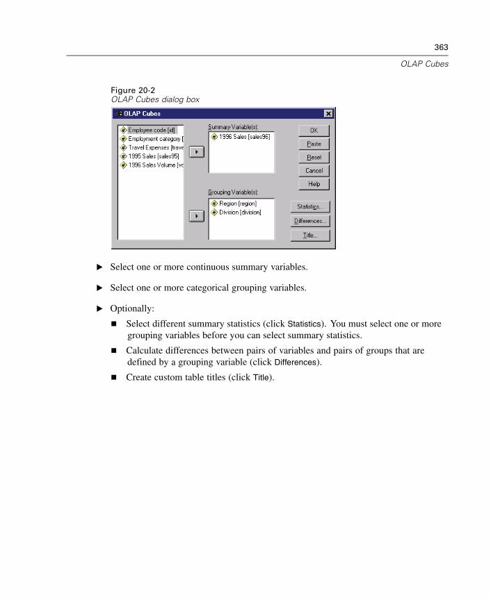
363

OLAP Cubes

Figure 20-2OLAP Cubes dialog box

E Select one or more continuous summary variables.

E Select one or more categorical grouping variables.

E Optionally:

Select different summary statistics (click Statistics). You must select one or moregrouping variables before you can select summary statistics.

Calculate differences between pairs of variables and pairs of groups that aredefined by a grouping variable (click Differences).

Create custom table titles (click Title).

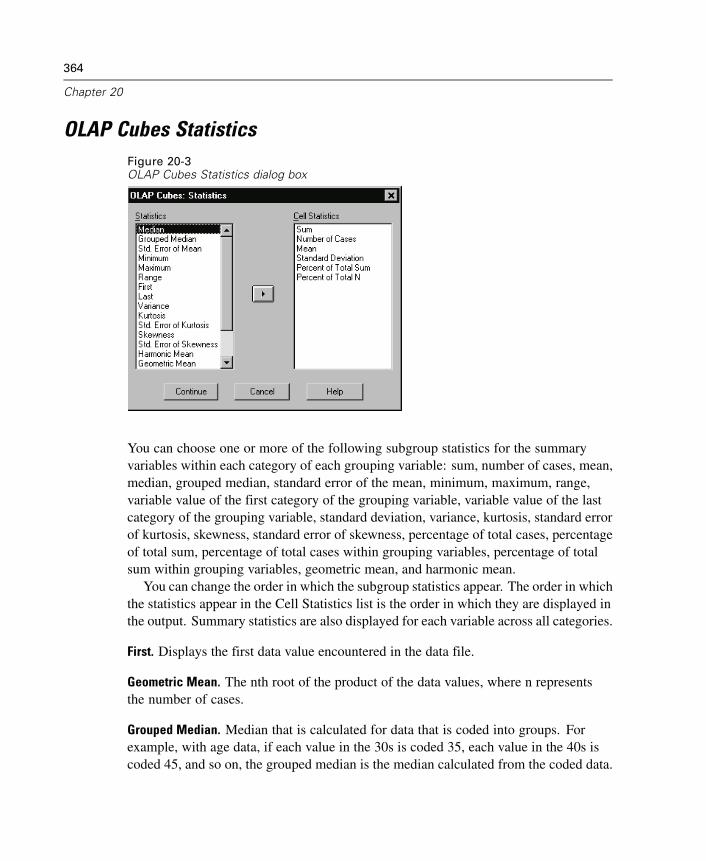
364

Chapter 20

OLAP Cubes StatisticsFigure 20-3OLAP Cubes Statistics dialog box

You can choose one or more of the following subgroup statistics for the summaryvariables within each category of each grouping variable: sum, number of cases, mean,median, grouped median, standard error of the mean, minimum, maximum, range,variable value of the first category of the grouping variable, variable value of the lastcategory of the grouping variable, standard deviation, variance, kurtosis, standard errorof kurtosis, skewness, standard error of skewness, percentage of total cases, percentageof total sum, percentage of total cases within grouping variables, percentage of totalsum within grouping variables, geometric mean, and harmonic mean.

You can change the order in which the subgroup statistics appear. The order in whichthe statistics appear in the Cell Statistics list is the order in which they are displayed inthe output. Summary statistics are also displayed for each variable across all categories.




365

OLAP Cubes









Percent of N in. Percentage of the number of cases for the specified grouping variablewithin categories of other grouping variables. If you only have one grouping variable,this value is identical to percentage of total number of cases.

Percent of Sum in. Percentage of the sum for the specified grouping variable withincategories of other grouping variables. If you only have one grouping variable, thisvalue is identical to percentage of total sum.

Percent of Total N. Percentage of the total number of cases in each category.

Percent of Total Sum. Percentage of the total sum in each category.


Skewness. A measure of the asymmetry of a distribution. The normal distribution issymmetric and has a skewness value of 0. A distribution with a significant positiveskewness has a long right tail. A distribution with a significant negative skewness has a

366

Chapter 20

long left tail. As a guideline, a skewness value more than twice its standard error istaken to indicate a departure from symmetry.





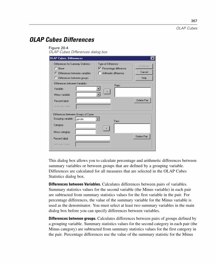
367

OLAP Cubes

OLAP Cubes DifferencesFigure 20-4OLAP Cubes Differences dialog box

This dialog box allows you to calculate percentage and arithmetic differences betweensummary variables or between groups that are defined by a grouping variable.Differences are calculated for all measures that are selected in the OLAP CubesStatistics dialog box.

Differences between Variables. Calculates differences between pairs of variables.Summary statistics values for the second variable (the Minus variable) in each pairare subtracted from summary statistics values for the first variable in the pair. Forpercentage differences, the value of the summary variable for the Minus variable isused as the denominator. You must select at least two summary variables in the maindialog box before you can specify differences between variables.

Differences between groups. Calculates differences between pairs of groups defined bya grouping variable. Summary statistics values for the second category in each pair (theMinus category) are subtracted from summary statistics values for the first category inthe pair. Percentage differences use the value of the summary statistic for the Minus

368

Chapter 20

category as the denominator. You must select one or more grouping variables in themain dialog box before you can specify differences between groups.

OLAP Cubes TitleFigure 20-5OLAP Cubes Title dialog box

You can change the title of your output or add a caption that will appear below theoutput table. You can also control line wrapping of titles and captions by typing \nwherever you want to insert a line break in the text.

Chapter

21T Tests

Three types of t tests are available:

Independent-samples t test (two-sample t test). Compares the means of one variable fortwo groups of cases. Descriptive statistics for each group and Levene’s test for equalityof variances are provided, as well as both equal- and unequal-variance t values anda 95% confidence interval for the difference in means.

Paired-samples t test (dependent t test). Compares the means of two variables for asingle group. This test is also for matched pairs or case-control study designs. Theoutput includes descriptive statistics for the test variables, the correlation betweenthe variables, descriptive statistics for the paired differences, the t test, and a 95%confidence interval.

One-sample t test. Compares the mean of one variable with a known or hypothesizedvalue. Descriptive statistics for the test variables are displayed along with the t test. A95% confidence interval for the difference between the mean of the test variable andthe hypothesized test value is part of the default output.

Independent-Samples T Test

The Independent-Samples T Test procedure compares means for two groups of cases.Ideally, for this test, the subjects should be randomly assigned to two groups, so thatany difference in response is due to the treatment (or lack of treatment) and not to otherfactors. This is not the case if you compare average income for males and females. Aperson is not randomly assigned to be a male or female. In such situations, you shouldensure that differences in other factors are not masking or enhancing a significantdifference in means. Differences in average income may be influenced by factorssuch as education (and not by sex alone).

369

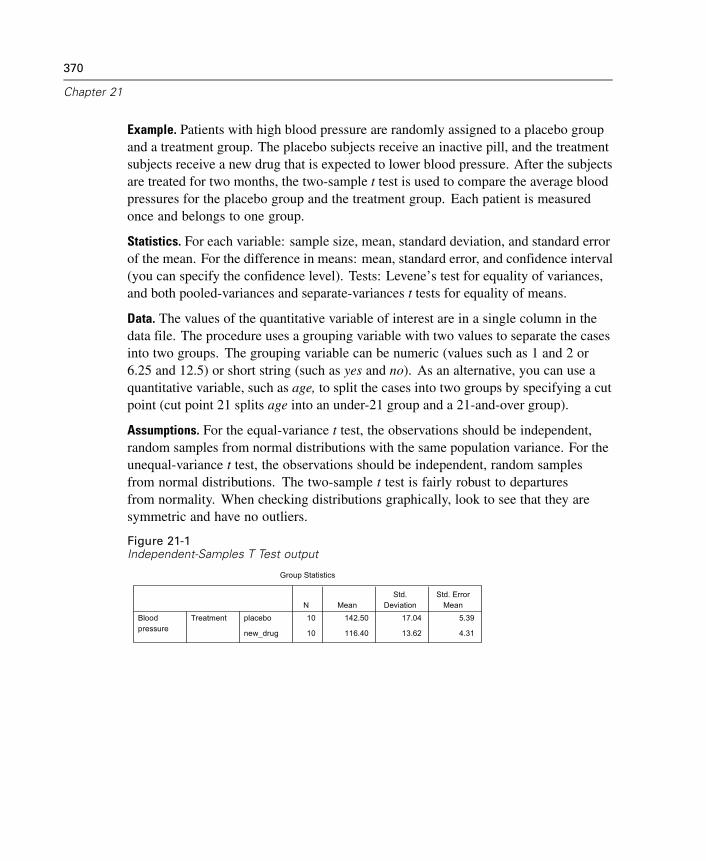
370

Chapter 21

Example. Patients with high blood pressure are randomly assigned to a placebo groupand a treatment group. The placebo subjects receive an inactive pill, and the treatmentsubjects receive a new drug that is expected to lower blood pressure. After the subjectsare treated for two months, the two-sample t test is used to compare the average bloodpressures for the placebo group and the treatment group. Each patient is measuredonce and belongs to one group.

Statistics. For each variable: sample size, mean, standard deviation, and standard errorof the mean. For the difference in means: mean, standard error, and confidence interval(you can specify the confidence level). Tests: Levene’s test for equality of variances,and both pooled-variances and separate-variances t tests for equality of means.

Data. The values of the quantitative variable of interest are in a single column in thedata file. The procedure uses a grouping variable with two values to separate the casesinto two groups. The grouping variable can be numeric (values such as 1 and 2 or6.25 and 12.5) or short string (such as yes and no). As an alternative, you can use aquantitative variable, such as age, to split the cases into two groups by specifying a cutpoint (cut point 21 splits age into an under-21 group and a 21-and-over group).

Assumptions. For the equal-variance t test, the observations should be independent,random samples from normal distributions with the same population variance. For theunequal-variance t test, the observations should be independent, random samplesfrom normal distributions. The two-sample t test is fairly robust to departuresfrom normality. When checking distributions graphically, look to see that they aresymmetric and have no outliers.

Figure 21-1Independent-Samples T Test output

10 142.50 17.04 5.39

10 116.40 13.62 4.31

placebo

new_drug

TreatmentBloodpressure

N MeanStd.

DeviationStd. Error

Mean

Group Statistics

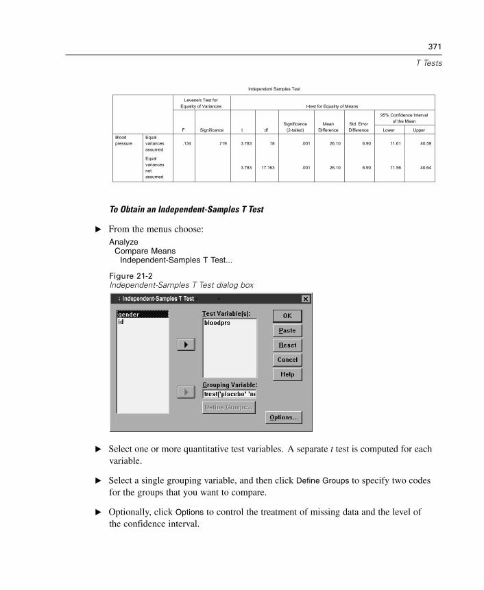
371

T Tests

.134 .719 3.783 18 .001 26.10 6.90 11.61 40.59

3.783 17.163 .001 26.10 6.90 11.56 40.64

Equalvariancesassumed

Equalvariancesnotassumed

Bloodpressure

F Significance

Levene's Test forEquality of Variances

t dfSignificance

(2-tailed)Mean

DifferenceStd. ErrorDifference Lower Upper

95% Confidence Intervalof the Mean

t-test for Equality of Means

Independent Samples Test

To Obtain an Independent-Samples T Test


Compare MeansIndependent-Samples T Test...

Figure 21-2Independent-Samples T Test dialog box

E Select one or more quantitative test variables. A separate t test is computed for eachvariable.

E Select a single grouping variable, and then click Define Groups to specify two codesfor the groups that you want to compare.

E Optionally, click Options to control the treatment of missing data and the level ofthe confidence interval.

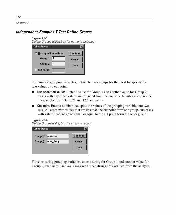
372

Chapter 21

Independent-Samples T Test Define GroupsFigure 21-3Define Groups dialog box for numeric variables

For numeric grouping variables, define the two groups for the t test by specifyingtwo values or a cut point:

Use specified values. Enter a value for Group 1 and another value for Group 2.Cases with any other values are excluded from the analysis. Numbers need not beintegers (for example, 6.25 and 12.5 are valid).

Cut point. Enter a number that splits the values of the grouping variable into twosets. All cases with values that are less than the cut point form one group, and caseswith values that are greater than or equal to the cut point form the other group.

Figure 21-4Define Groups dialog box for string variables

For short string grouping variables, enter a string for Group 1 and another value forGroup 2, such as yes and no. Cases with other strings are excluded from the analysis.

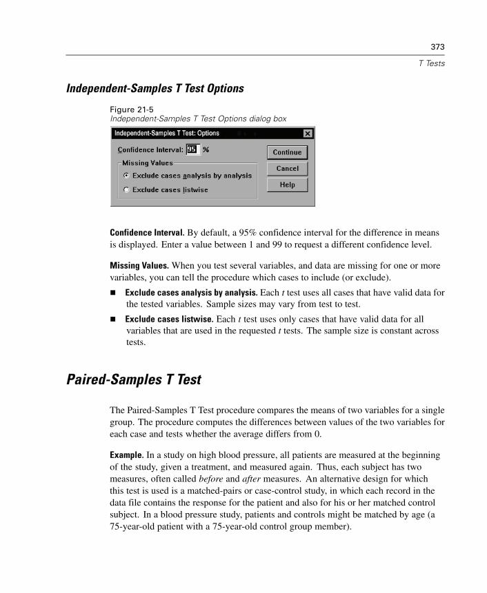
373

T Tests

Independent-Samples T Test Options

Figure 21-5Independent-Samples T Test Options dialog box

Confidence Interval. By default, a 95% confidence interval for the difference in meansis displayed. Enter a value between 1 and 99 to request a different confidence level.

Missing Values. When you test several variables, and data are missing for one or morevariables, you can tell the procedure which cases to include (or exclude).

Exclude cases analysis by analysis. Each t test uses all cases that have valid data forthe tested variables. Sample sizes may vary from test to test.

Exclude cases listwise. Each t test uses only cases that have valid data for allvariables that are used in the requested t tests. The sample size is constant acrosstests.

Paired-Samples T Test

The Paired-Samples T Test procedure compares the means of two variables for a singlegroup. The procedure computes the differences between values of the two variables foreach case and tests whether the average differs from 0.

Example. In a study on high blood pressure, all patients are measured at the beginningof the study, given a treatment, and measured again. Thus, each subject has twomeasures, often called before and after measures. An alternative design for whichthis test is used is a matched-pairs or case-control study, in which each record in thedata file contains the response for the patient and also for his or her matched controlsubject. In a blood pressure study, patients and controls might be matched by age (a75-year-old patient with a 75-year-old control group member).

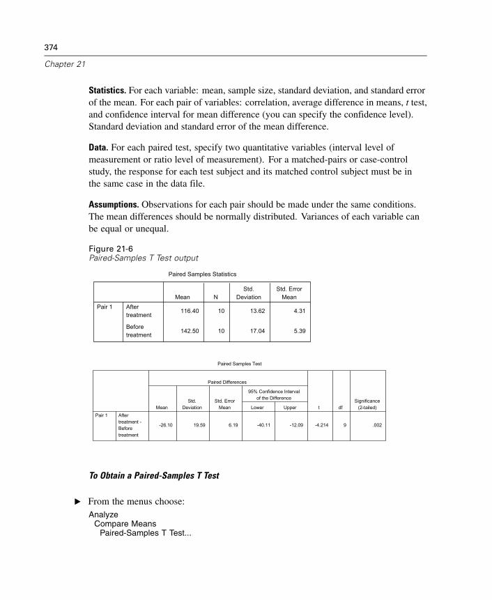
374

Chapter 21

Statistics. For each variable: mean, sample size, standard deviation, and standard errorof the mean. For each pair of variables: correlation, average difference in means, t test,and confidence interval for mean difference (you can specify the confidence level).Standard deviation and standard error of the mean difference.

Data. For each paired test, specify two quantitative variables (interval level ofmeasurement or ratio level of measurement). For a matched-pairs or case-controlstudy, the response for each test subject and its matched control subject must be inthe same case in the data file.

Assumptions. Observations for each pair should be made under the same conditions.The mean differences should be normally distributed. Variances of each variable canbe equal or unequal.

Figure 21-6Paired-Samples T Test output

116.40 10 13.62 4.31

142.50 10 17.04 5.39

Aftertreatment

Beforetreatment

Pair 1Mean N

Std.Deviation

Std. ErrorMean

Paired Samples Statistics

-26.10 19.59 6.19 -40.11 -12.09 -4.214 9 .002

Aftertreatment -Beforetreatment

Pair 1Mean

Std.Deviation

Std. ErrorMean Lower Upper

95% Confidence Intervalof the Difference

Paired Differences

t dfSignificance

(2-tailed)

Paired Samples Test

To Obtain a Paired-Samples T Test


Compare MeansPaired-Samples T Test...

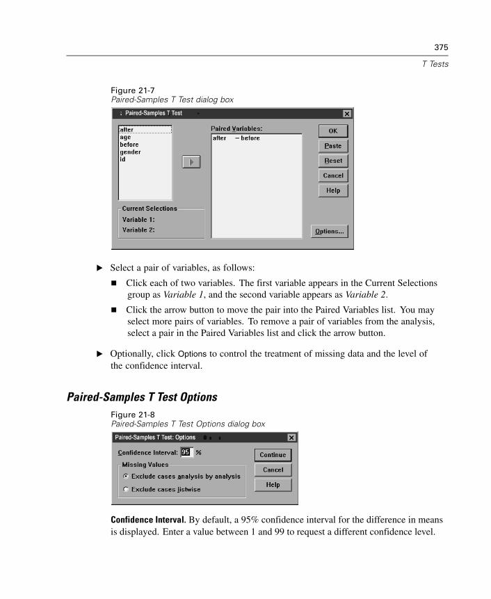
375

T Tests

Figure 21-7Paired-Samples T Test dialog box

E Select a pair of variables, as follows:

Click each of two variables. The first variable appears in the Current Selectionsgroup as Variable 1, and the second variable appears as Variable 2.

Click the arrow button to move the pair into the Paired Variables list. You mayselect more pairs of variables. To remove a pair of variables from the analysis,select a pair in the Paired Variables list and click the arrow button.


Paired-Samples T Test OptionsFigure 21-8Paired-Samples T Test Options dialog box

Confidence Interval. By default, a 95% confidence interval for the difference in meansis displayed. Enter a value between 1 and 99 to request a different confidence level.

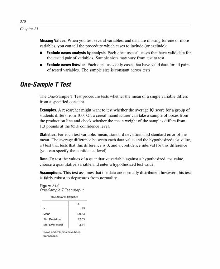
376

Chapter 21

Missing Values. When you test several variables, and data are missing for one or morevariables, you can tell the procedure which cases to include (or exclude):

Exclude cases analysis by analysis. Each t test uses all cases that have valid data forthe tested pair of variables. Sample sizes may vary from test to test.

Exclude cases listwise. Each t test uses only cases that have valid data for all pairsof tested variables. The sample size is constant across tests.

One-Sample T Test

The One-Sample T Test procedure tests whether the mean of a single variable differsfrom a specified constant.

Examples. A researcher might want to test whether the average IQ score for a group ofstudents differs from 100. Or, a cereal manufacturer can take a sample of boxes fromthe production line and check whether the mean weight of the samples differs from1.3 pounds at the 95% confidence level.

Statistics. For each test variable: mean, standard deviation, and standard error of themean. The average difference between each data value and the hypothesized test value,a t test that tests that this difference is 0, and a confidence interval for this difference(you can specify the confidence level).

Data. To test the values of a quantitative variable against a hypothesized test value,choose a quantitative variable and enter a hypothesized test value.

Assumptions. This test assumes that the data are normally distributed; however, this testis fairly robust to departures from normality.

Figure 21-9One-Sample T Test output

15

109.33

12.03

3.11

N

Mean

Std. Deviation

Std. Error Mean

IQ

One-Sample Statistics

Rows and columns have beentransposed.

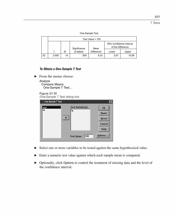
377

T Tests

3.005 14 .009 9.33 2.67 15.99IQt df

Significance(2-tailed)

MeanDifference Lower Upper

95% Confidence Intervalof the Difference

Test Value = 100

One-Sample Test

To Obtain a One-Sample T Test


Compare MeansOne-Sample T Test...

Figure 21-10One-Sample T Test dialog box

E Select one or more variables to be tested against the same hypothesized value.

E Enter a numeric test value against which each sample mean is compared.


378

Chapter 21

One-Sample T Test OptionsFigure 21-11One-Sample T Test Options dialog box

Confidence Interval. By default, a 95% confidence interval for the difference betweenthe mean and the hypothesized test value is displayed. Enter a value between 1 and 99to request a different confidence level.

Missing Values. When you test several variables, and data are missing for one or morevariables, you can tell the procedure which cases to include (or exclude).

Exclude cases analysis by analysis. Each t test uses all cases that have valid data forthe tested variable. Sample sizes may vary from test to test.

Exclude cases listwise. Each t test uses only cases that have valid data for allvariables that are used in any of the requested t tests. The sample size is constantacross tests.

T-TEST Command Additional Features

The SPSS command language also allows you to:

Produce both one-sample and independent-samples t tests by running a singlecommand.

Test a variable against each variable on a list, in a paired t test (with the PAIRSsubcommand).


Chapter

22One-Way ANOVA

The One-Way ANOVA procedure produces a one-way analysis of variance for aquantitative dependent variable by a single factor (independent) variable. Analysis ofvariance is used to test the hypothesis that several means are equal. This techniqueis an extension of the two-sample t test.

In addition to determining that differences exist among the means, you may want toknow which means differ. There are two types of tests for comparing means: a prioricontrasts and post hoc tests. Contrasts are tests set up before running the experiment,and post hoc tests are run after the experiment has been conducted. You can alsotest for trends across categories.

Example. Doughnuts absorb fat in various amounts when they are cooked. Anexperiment is set up involving three types of fat: peanut oil, corn oil, and lard. Peanutoil and corn oil are unsaturated fats, and lard is a saturated fat. Along with determiningwhether the amount of fat absorbed depends on the type of fat used, you could setup an a priori contrast to determine whether the amount of fat absorption differs forsaturated and unsaturated fats.

Statistics. For each group: number of cases, mean, standard deviation, standard error ofthe mean, minimum, maximum, and 95%-confidence interval for the mean. Levene’stest for homogeneity of variance, analysis-of-variance table and robust tests of theequality of means for each dependent variable, user-specified a priori contrasts, andpost hoc range tests and multiple comparisons: Bonferroni, Sidak, Tukey’s honestlysignificant difference, Hochberg’s GT2, Gabriel, Dunnett, Ryan-Einot-Gabriel-WelschF test (R-E-G-W F), Ryan-Einot-Gabriel-Welsch range test (R-E-G-W Q),Tamhane’s T2, Dunnett’s T3, Games-Howell, Dunnett’s C, Duncan’s multiple rangetest, Student-Newman-Keuls (S-N-K), Tukey’s b, Waller-Duncan, Scheffé, andleast-significant difference.

Data. Factor variable values should be integers, and the dependent variable should bequantitative (interval level of measurement).

379

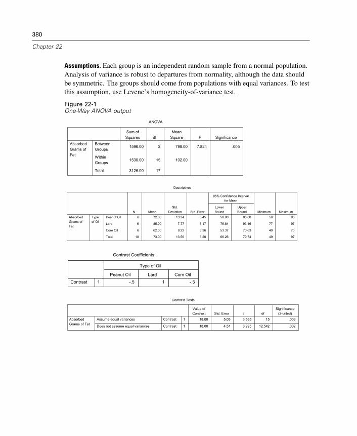
380

Chapter 22

Assumptions. Each group is an independent random sample from a normal population.Analysis of variance is robust to departures from normality, although the data shouldbe symmetric. The groups should come from populations with equal variances. To testthis assumption, use Levene’s homogeneity-of-variance test.

Figure 22-1One-Way ANOVA output

1596.00 2 798.00 7.824 .005

1530.00 15 102.00

3126.00 17

BetweenGroups

WithinGroups

Total

AbsorbedGrams ofFat

Sum ofSquares df

MeanSquare F Significance

ANOVA

6 72.00 13.34 5.45 58.00 86.00 56 95

6 85.00 7.77 3.17 76.84 93.16 77 97

6 62.00 8.22 3.36 53.37 70.63 49 70

18 73.00 13.56 3.20 66.26 79.74 49 97

Peanut Oil

Lard

Corn Oil

Total

Typeof Oil

AbsorbedGrams ofFat

N MeanStd.

Deviation Std. ErrorLowerBound

UpperBound

95% Confidence Intervalfor Mean

Minimum Maximum

Descriptives

-.5 1 -.51ContrastPeanut Oil Lard Corn Oil

Type of Oil

Contrast Coefficients

18.00 5.05 3.565 15 .003

18.00 4.51 3.995 12.542 .002

1Contrast

1Contrast

Assume equal variances

Does not assume equal variances

AbsorbedGrams of Fat

Value ofContrast Std. Error t df


Contrast Tests

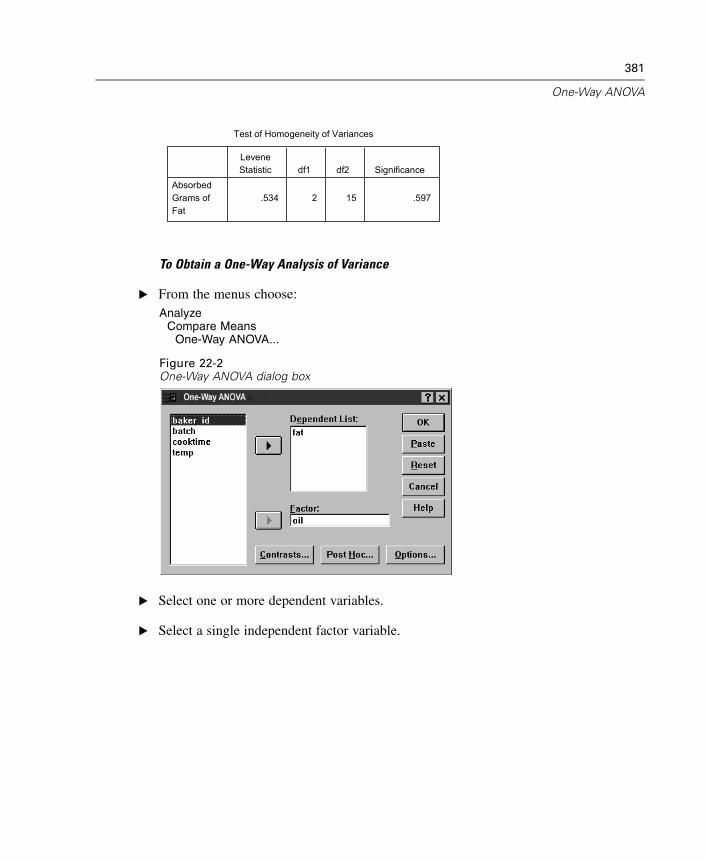
381

One-Way ANOVA

.534 2 15 .597AbsorbedGrams ofFat

LeveneStatistic df1 df2 Significance

Test of Homogeneity of Variances

To Obtain a One-Way Analysis of Variance


Compare MeansOne-Way ANOVA...

Figure 22-2One-Way ANOVA dialog box


E Select a single independent factor variable.

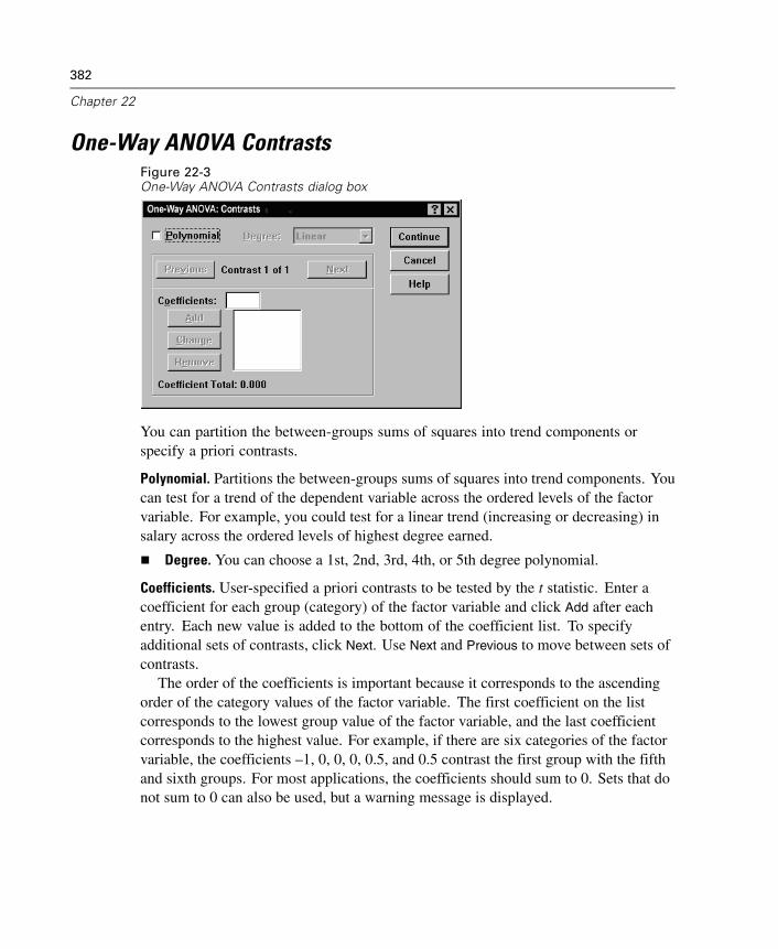
382

Chapter 22

One-Way ANOVA ContrastsFigure 22-3One-Way ANOVA Contrasts dialog box

You can partition the between-groups sums of squares into trend components orspecify a priori contrasts.

Polynomial. Partitions the between-groups sums of squares into trend components. Youcan test for a trend of the dependent variable across the ordered levels of the factorvariable. For example, you could test for a linear trend (increasing or decreasing) insalary across the ordered levels of highest degree earned.

Degree. You can choose a 1st, 2nd, 3rd, 4th, or 5th degree polynomial.

Coefficients. User-specified a priori contrasts to be tested by the t statistic. Enter acoefficient for each group (category) of the factor variable and click Add after eachentry. Each new value is added to the bottom of the coefficient list. To specifyadditional sets of contrasts, click Next. Use Next and Previous to move between sets ofcontrasts.

The order of the coefficients is important because it corresponds to the ascendingorder of the category values of the factor variable. The first coefficient on the listcorresponds to the lowest group value of the factor variable, and the last coefficientcorresponds to the highest value. For example, if there are six categories of the factorvariable, the coefficients –1, 0, 0, 0, 0.5, and 0.5 contrast the first group with the fifthand sixth groups. For most applications, the coefficients should sum to 0. Sets that donot sum to 0 can also be used, but a warning message is displayed.

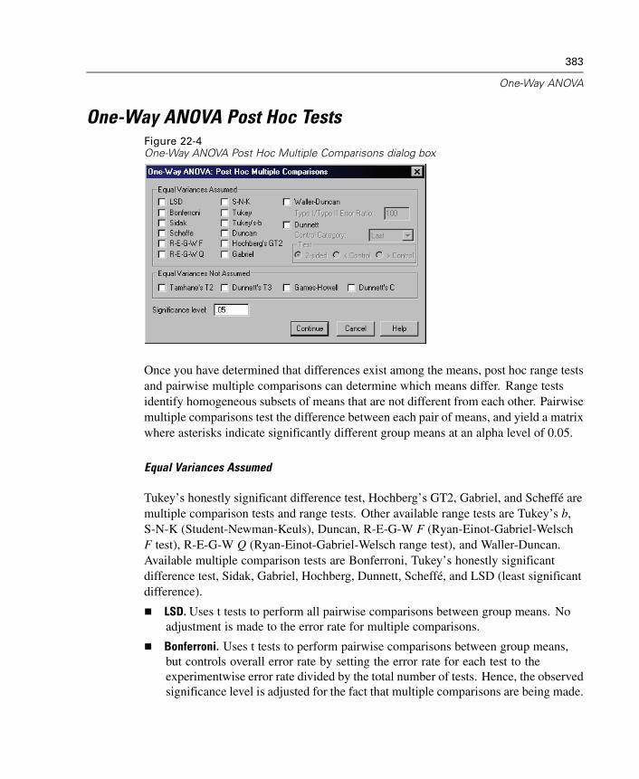
383

One-Way ANOVA

One-Way ANOVA Post Hoc TestsFigure 22-4One-Way ANOVA Post Hoc Multiple Comparisons dialog box

Once you have determined that differences exist among the means, post hoc range testsand pairwise multiple comparisons can determine which means differ. Range testsidentify homogeneous subsets of means that are not different from each other. Pairwisemultiple comparisons test the difference between each pair of means, and yield a matrixwhere asterisks indicate significantly different group means at an alpha level of 0.05.

Equal Variances Assumed

Tukey’s honestly significant difference test, Hochberg’s GT2, Gabriel, and Scheffé aremultiple comparison tests and range tests. Other available range tests are Tukey’s b,S-N-K (Student-Newman-Keuls), Duncan, R-E-G-W F (Ryan-Einot-Gabriel-WelschF test), R-E-G-W Q (Ryan-Einot-Gabriel-Welsch range test), and Waller-Duncan.Available multiple comparison tests are Bonferroni, Tukey’s honestly significantdifference test, Sidak, Gabriel, Hochberg, Dunnett, Scheffé, and LSD (least significantdifference).

LSD. Uses t tests to perform all pairwise comparisons between group means. Noadjustment is made to the error rate for multiple comparisons.

Bonferroni. Uses t tests to perform pairwise comparisons between group means,but controls overall error rate by setting the error rate for each test to theexperimentwise error rate divided by the total number of tests. Hence, the observedsignificance level is adjusted for the fact that multiple comparisons are being made.

384

Chapter 22

Sidak. Pairwise multiple comparison test based on a t statistic. Sidak adjusts thesignificance level for multiple comparisons and provides tighter bounds thanBonferroni.

Scheffe. Performs simultaneous joint pairwise comparisons for all possible pairwisecombinations of means. Uses the F sampling distribution. Can be used to examineall possible linear combinations of group means, not just pairwise comparisons.

R-E-G-W F. Ryan-Einot-Gabriel-Welsch multiple stepdown procedure based onan F test.

R-E-G-W Q. Ryan-Einot-Gabriel-Welsch multiple stepdown procedure based onthe Studentized range.

S-N-K. Makes all pairwise comparisons between means using the Studentizedrange distribution. With equal sample sizes, it also compares pairs of means withinhomogeneous subsets, using a stepwise procedure. Means are ordered fromhighest to lowest, and extreme differences are tested first.

Tukey. Uses the Studentized range statistic to make all of the pairwise comparisonsbetween groups. Sets the experimentwise error rate at the error rate for thecollection for all pairwise comparisons.

Tukey's-b. Uses the Studentized range distribution to make pairwise comparisonsbetween groups. The critical value is the average of the corresponding value forthe Tukey's honestly significant difference test and the Student-Newman-Keuls.

Duncan. Makes pairwise comparisons using a stepwise order of comparisonsidentical to the order used by the Student-Newman-Keuls test, but sets a protectionlevel for the error rate for the collection of tests, rather than an error rate forindividual tests. Uses the Studentized range statistic.

Hochberg's GT2. Multiple comparison and range test that uses the Studentizedmaximum modulus. Similar to Tukey's honestly significant difference test.

Gabriel. Pairwise comparison test that used the Studentized maximum modulus andis generally more powerful than Hochberg's GT2 when the cell sizes are unequal.Gabriel's test may become liberal when the cell sizes vary greatly.

Waller-Duncan. Multiple comparison test based on a t statistic; uses a Bayesianapproach.

Dunnett. Pairwise multiple comparison t test that compares a set of treatmentsagainst a single control mean. The last category is the default control category.Alternatively, you can choose the first category. 2-sided tests that the mean at anylevel (except the control category) of the factor is not equal to that of the control

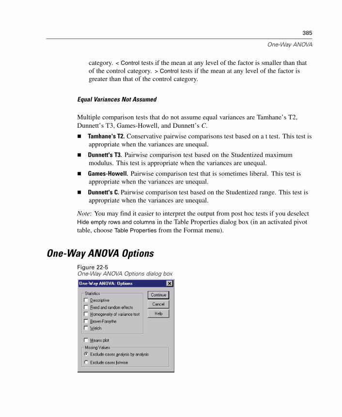
385

One-Way ANOVA

category. < Control tests if the mean at any level of the factor is smaller than thatof the control category. > Control tests if the mean at any level of the factor isgreater than that of the control category.

Equal Variances Not Assumed

Multiple comparison tests that do not assume equal variances are Tamhane’s T2,Dunnett’s T3, Games-Howell, and Dunnett’s C.

Tamhane's T2. Conservative pairwise comparisons test based on a t test. This test isappropriate when the variances are unequal.

Dunnett's T3. Pairwise comparison test based on the Studentized maximummodulus. This test is appropriate when the variances are unequal.

Games-Howell. Pairwise comparison test that is sometimes liberal. This test isappropriate when the variances are unequal.

Dunnett's C. Pairwise comparison test based on the Studentized range. This test isappropriate when the variances are unequal.

Note: You may find it easier to interpret the output from post hoc tests if you deselectHide empty rows and columns in the Table Properties dialog box (in an activated pivottable, choose Table Properties from the Format menu).

One-Way ANOVA OptionsFigure 22-5One-Way ANOVA Options dialog box

386

Chapter 22

Statistics. Choose one or more of the following:

Descriptive. Calculates the number of cases, mean, standard deviation, standarderror of the mean, minimum, maximum, and 95%-confidence intervals for eachdependent variable for each group.

Fixed and random effects. Displays the standard deviation, standard error, and95%-confidence interval for the fixed-effects model, and the standard error,95%-confidence interval, and estimate of between-components variance for therandom-effects model.

Homogeneity of variance test. Calculates the Levene statistic to test for the equalityof group variances. This test is not dependent on the assumption of normality.

Brown-Forsythe. Calculates the Brown-Forsythe statistic to test for the equality ofgroup means. This statistic is preferable to the F statistic when the assumption ofequal variances does not hold.

Welch. Calculates the Welch statistic to test for the equality of group means. Thisstatistic is preferable to the F statistic when the assumption of equal variancesdoes not hold.

Means plot. Displays a chart that plots the subgroup means (the means for each groupdefined by values of the factor variable).


Exclude cases analysis by analysis. A case with a missing value for either thedependent or the factor variable for a given analysis is not used in that analysis.Also, a case outside the range specified for the factor variable is not used.

Exclude cases listwise. Cases with missing values for the factor variable or forany dependent variable included on the dependent list in the main dialog box areexcluded from all analyses. If you have not specified multiple dependent variables,this has no effect.

ONEWAY Command Additional Features


Obtain fixed- and random-effects statistics. Standard deviation, standard error ofthe mean, and 95% confidence intervals for the fixed-effects model. Standarderror, 95% confidence intervals, and estimate of between-components variance forrandom-effects model (using STATISTICS=EFFECTS).

387

One-Way ANOVA

Specify alpha levels for the least significance difference, Bonferroni, Duncan, andScheffé multiple comparison tests (with the RANGES subcommand).

Write a matrix of means, standard deviations, and frequencies, or read a matrixof means, frequencies, pooled variances, and degrees of freedom for the pooledvariances. These matrices can be used in place of raw data to obtain a one-wayanalysis of variance (with the MATRIX subcommand).


Chapter

23GLM Univariate Analysis

The GLM Univariate procedure provides regression analysis and analysis of variancefor one dependent variable by one or more factors and/or variables. The factor variablesdivide the population into groups. Using this General Linear Model procedure, youcan test null hypotheses about the effects of other variables on the means of variousgroupings of a single dependent variable. You can investigate interactions betweenfactors as well as the effects of individual factors, some of which may be random.In addition, the effects of covariates and covariate interactions with factors can beincluded. For regression analysis, the independent (predictor) variables are specifiedas covariates.

Both balanced and unbalanced models can be tested. A design is balanced if eachcell in the model contains the same number of cases. In addition to testing hypotheses,GLM Univariate produces estimates of parameters.

Commonly used a priori contrasts are available to perform hypothesis testing.Additionally, after an overall F test has shown significance, you can use post hoc tests toevaluate differences among specific means. Estimated marginal means give estimatesof predicted mean values for the cells in the model, and profile plots (interaction plots)of these means allow you to easily visualize some of the relationships.

Residuals, predicted values, Cook’s distance, and leverage values can be saved asnew variables in your data file for checking assumptions.

WLS Weight allows you to specify a variable used to give observations differentweights for a weighted least-squares (WLS) analysis, perhaps to compensate for adifferent precision of measurement.

Example. Data are gathered for individual runners in the Chicago marathon for severalyears. The time in which each runner finishes is the dependent variable. Other factorsinclude weather (cold, pleasant, or hot), number of months of training, number ofprevious marathons, and gender. Age is considered a covariate. You might findthat gender is a significant effect and that the interaction of gender with weatheris significant.

389

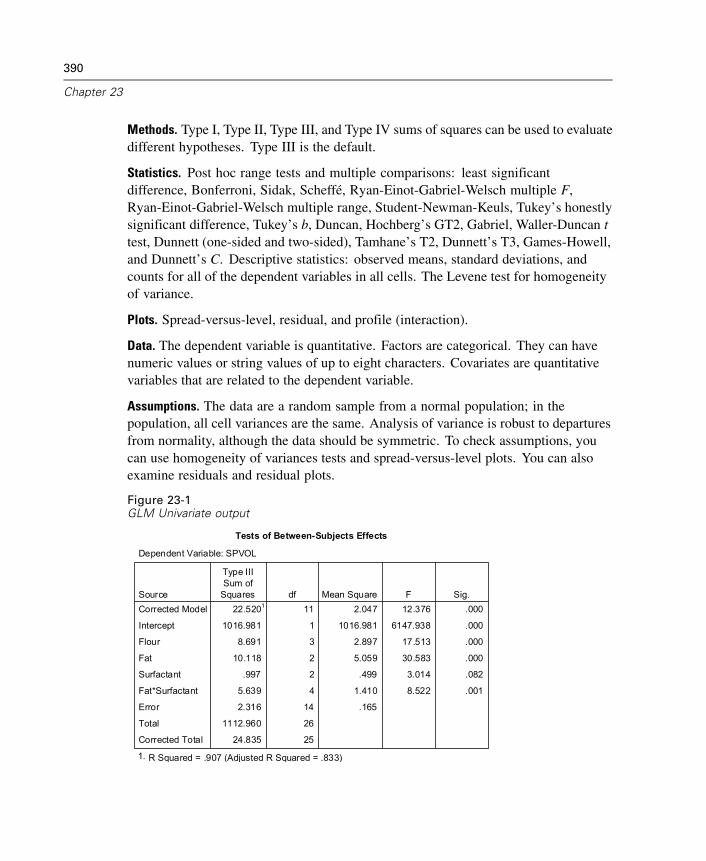
390

Chapter 23

Methods. Type I, Type II, Type III, and Type IV sums of squares can be used to evaluatedifferent hypotheses. Type III is the default.

Statistics. Post hoc range tests and multiple comparisons: least significantdifference, Bonferroni, Sidak, Scheffé, Ryan-Einot-Gabriel-Welsch multiple F,Ryan-Einot-Gabriel-Welsch multiple range, Student-Newman-Keuls, Tukey’s honestlysignificant difference, Tukey’s b, Duncan, Hochberg’s GT2, Gabriel, Waller-Duncan ttest, Dunnett (one-sided and two-sided), Tamhane’s T2, Dunnett’s T3, Games-Howell,and Dunnett’s C. Descriptive statistics: observed means, standard deviations, andcounts for all of the dependent variables in all cells. The Levene test for homogeneityof variance.

Plots. Spread-versus-level, residual, and profile (interaction).

Data. The dependent variable is quantitative. Factors are categorical. They can havenumeric values or string values of up to eight characters. Covariates are quantitativevariables that are related to the dependent variable.

Assumptions. The data are a random sample from a normal population; in thepopulation, all cell variances are the same. Analysis of variance is robust to departuresfrom normality, although the data should be symmetric. To check assumptions, youcan use homogeneity of variances tests and spread-versus-level plots. You can alsoexamine residuals and residual plots.

Figure 23-1GLM Univariate output

Tests of Between-Subjects Effects

Dependent Variable: SPVOL

22.5201 11 2.047 12.376 .000

1016.981 1 1016.981 6147.938 .000

8.691 3 2.897 17.513 .000

10.118 2 5.059 30.583 .000

.997 2 .499 3.014 .082

5.639 4 1.410 8.522 .001

2.316 14 .165

1112.960 26

24.835 25

SourceCorrected Model

Intercept

Flour

Fat

Surfactant

Fat*Surfactant

Error

Total

Corrected Total

Type IIISum of

Squares df Mean Square F Sig.

R Squared = .907 (Adjusted R Squared = .833)1.

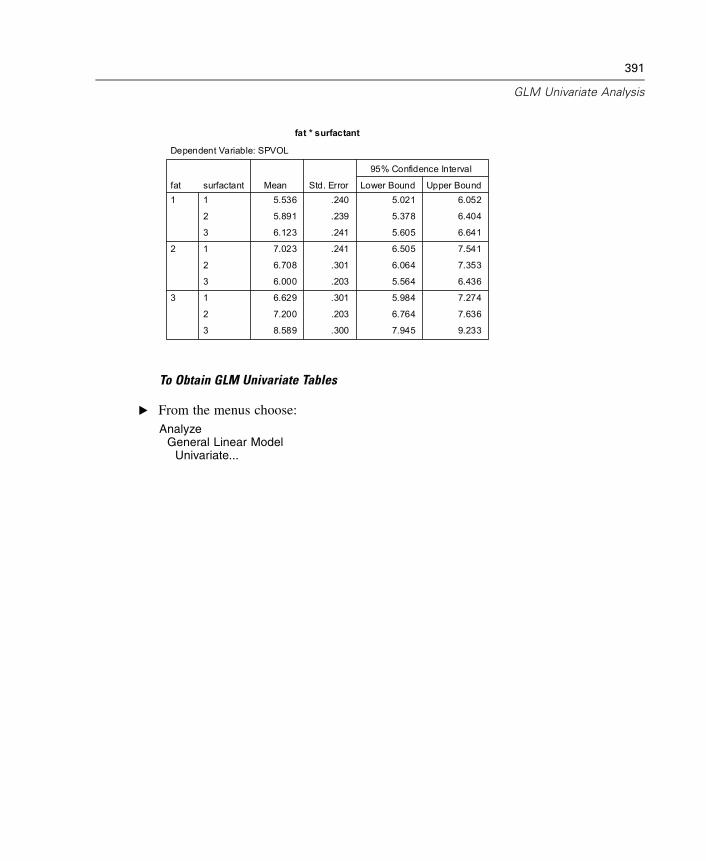
391

GLM Univariate Analysis

fat * surfactant

Dependent Variable: SPVOL

5.536 .240 5.021 6.052

5.891 .239 5.378 6.404

6.123 .241 5.605 6.641

7.023 .241 6.505 7.541

6.708 .301 6.064 7.353

6.000 .203 5.564 6.436

6.629 .301 5.984 7.274

7.200 .203 6.764 7.636

8.589 .300 7.945 9.233

surfactant1

2

3

1

2

3

1

2

3

fat1

2

3

Mean Std. Error Lower Bound Upper Bound

95% Confidence Interval

To Obtain GLM Univariate Tables


General Linear ModelUnivariate...

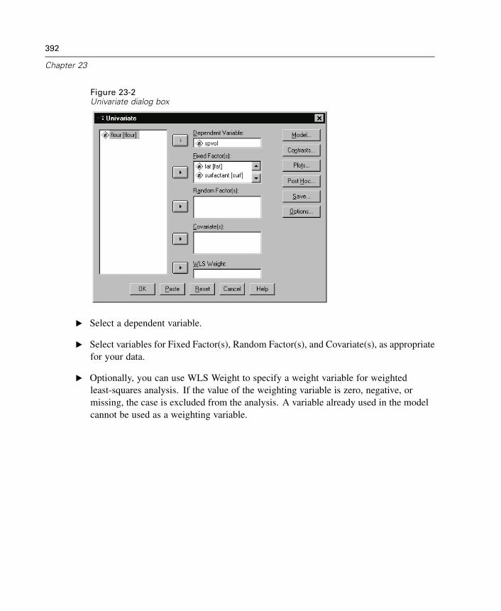
392

Chapter 23

Figure 23-2Univariate dialog box

E Select a dependent variable.

E Select variables for Fixed Factor(s), Random Factor(s), and Covariate(s), as appropriatefor your data.

E Optionally, you can use WLS Weight to specify a weight variable for weightedleast-squares analysis. If the value of the weighting variable is zero, negative, ormissing, the case is excluded from the analysis. A variable already used in the modelcannot be used as a weighting variable.

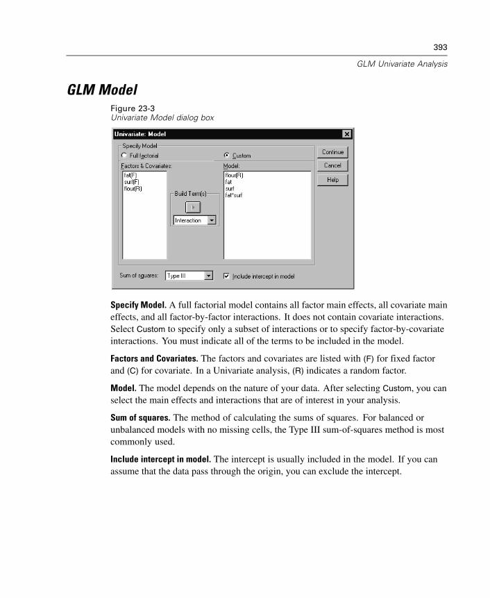
393


GLM ModelFigure 23-3Univariate Model dialog box

Specify Model. A full factorial model contains all factor main effects, all covariate maineffects, and all factor-by-factor interactions. It does not contain covariate interactions.Select Custom to specify only a subset of interactions or to specify factor-by-covariateinteractions. You must indicate all of the terms to be included in the model.

Factors and Covariates. The factors and covariates are listed with (F) for fixed factorand (C) for covariate. In a Univariate analysis, (R) indicates a random factor.

Model. The model depends on the nature of your data. After selecting Custom, you canselect the main effects and interactions that are of interest in your analysis.

Sum of squares. The method of calculating the sums of squares. For balanced orunbalanced models with no missing cells, the Type III sum-of-squares method is mostcommonly used.

Include intercept in model. The intercept is usually included in the model. If you canassume that the data pass through the origin, you can exclude the intercept.

394

Chapter 23

Build Terms

For the selected factors and covariates:

Interaction. Creates the highest-level interaction term of all selected variables. Thisis the default.

Main effects. Creates a main-effects term for each variable selected.

All 2-way. Creates all possible two-way interactions of the selected variables.

All 3-way. Creates all possible three-way interactions of the selected variables.

All 4-way. Creates all possible four-way interactions of the selected variables.

All 5-way. Creates all possible five-way interactions of the selected variables.

Sum of Squares

For the model, you can choose a type of sums of squares. Type III is the mostcommonly used and is the default.

Type I. This method is also known as the hierarchical decomposition of thesum-of-squares method. Each term is adjusted for only the term that precedes it in themodel. Type I sums of squares are commonly used for:

A balanced ANOVA model in which any main effects are specified before anyfirst-order interaction effects, any first-order interaction effects are specified beforeany second-order interaction effects, and so on.

A polynomial regression model in which any lower-order terms are specifiedbefore any higher-order terms.

A purely nested model in which the first-specified effect is nested within thesecond-specified effect, the second-specified effect is nested within the third, andso on. (This form of nesting can be specified only by using syntax.)

Type II. This method calculates the sums of squares of an effect in the model adjustedfor all other “appropriate” effects. An appropriate effect is one that corresponds to alleffects that do not contain the effect being examined. The Type II sum-of-squaresmethod is commonly used for:

A balanced ANOVA model.

Any model that has main factor effects only.

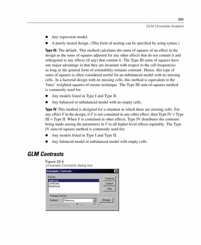
395


Any regression model.

A purely nested design. (This form of nesting can be specified by using syntax.)

Type III. The default. This method calculates the sums of squares of an effect in thedesign as the sums of squares adjusted for any other effects that do not contain it andorthogonal to any effects (if any) that contain it. The Type III sums of squares haveone major advantage in that they are invariant with respect to the cell frequenciesas long as the general form of estimability remains constant. Hence, this type ofsums of squares is often considered useful for an unbalanced model with no missingcells. In a factorial design with no missing cells, this method is equivalent to theYates’ weighted-squares-of-means technique. The Type III sum-of-squares methodis commonly used for:

Any models listed in Type I and Type II.

Any balanced or unbalanced model with no empty cells.

Type IV. This method is designed for a situation in which there are missing cells. Forany effect F in the design, if F is not contained in any other effect, then Type IV = TypeIII = Type II. When F is contained in other effects, Type IV distributes the contrastsbeing made among the parameters in F to all higher-level effects equitably. The TypeIV sum-of-squares method is commonly used for:

Any models listed in Type I and Type II.

Any balanced model or unbalanced model with empty cells.

GLM ContrastsFigure 23-4Univariate Contrasts dialog box

396

Chapter 23

Contrasts are used to test for differences among the levels of a factor. You can specifya contrast for each factor in the model (in a repeated measures model, for eachbetween-subjects factor). Contrasts represent linear combinations of the parameters.

Hypothesis testing is based on the null hypothesis LB = 0, where L is the contrastcoefficients matrix and B is the parameter vector. When a contrast is specified, SPSScreates an L matrix in which the columns corresponding to the factor match thecontrast. The remaining columns are adjusted so that the L matrix is estimable.

The output includes an F statistic for each set of contrasts. Also displayed for thecontrast differences are Bonferroni-type simultaneous confidence intervals based onStudent’s t distribution.

Available Contrasts

Available contrasts are deviation, simple, difference, Helmert, repeated, andpolynomial. For deviation contrasts and simple contrasts, you can choose whether thereference category is the last or first category.

Contrast Types

Deviation. Compares the mean of each level (except a reference category) to the meanof all of the levels (grand mean). The levels of the factor can be in any order.

Simple. Compares the mean of each level to the mean of a specified level. This typeof contrast is useful when there is a control group. You can choose the first or lastcategory as the reference.

Difference. Compares the mean of each level (except the first) to the mean of previouslevels. (Sometimes called reverse Helmert contrasts.)

Helmert. Compares the mean of each level of the factor (except the last) to the mean ofsubsequent levels.

Repeated. Compares the mean of each level (except the last) to the mean of thesubsequent level.

Polynomial. Compares the linear effect, quadratic effect, cubic effect, and so on. Thefirst degree of freedom contains the linear effect across all categories; the seconddegree of freedom, the quadratic effect; and so on. These contrasts are often usedto estimate polynomial trends.

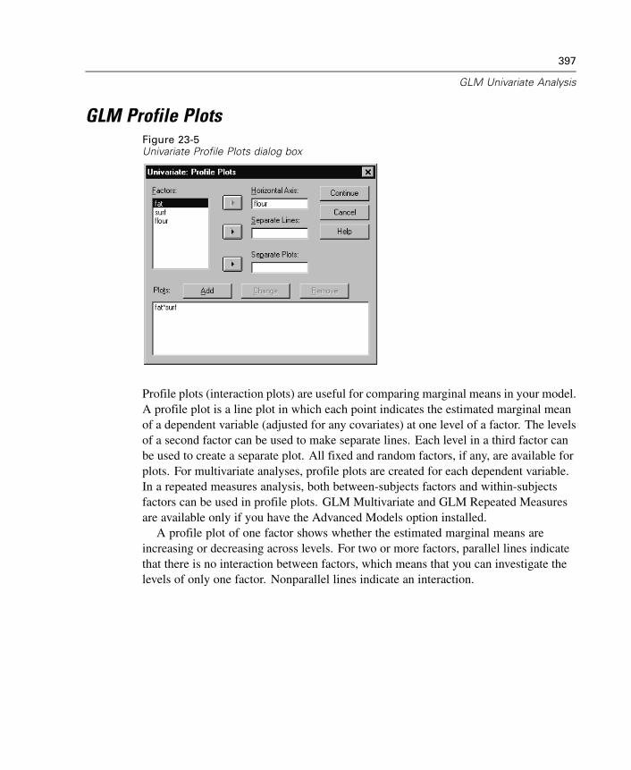
397


GLM Profile PlotsFigure 23-5Univariate Profile Plots dialog box

Profile plots (interaction plots) are useful for comparing marginal means in your model.A profile plot is a line plot in which each point indicates the estimated marginal meanof a dependent variable (adjusted for any covariates) at one level of a factor. The levelsof a second factor can be used to make separate lines. Each level in a third factor canbe used to create a separate plot. All fixed and random factors, if any, are available forplots. For multivariate analyses, profile plots are created for each dependent variable.In a repeated measures analysis, both between-subjects factors and within-subjectsfactors can be used in profile plots. GLM Multivariate and GLM Repeated Measuresare available only if you have the Advanced Models option installed.

A profile plot of one factor shows whether the estimated marginal means areincreasing or decreasing across levels. For two or more factors, parallel lines indicatethat there is no interaction between factors, which means that you can investigate thelevels of only one factor. Nonparallel lines indicate an interaction.

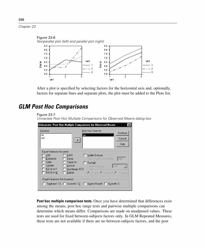
398

Chapter 23

Figure 23-6Nonparallel plot (left) and parallel plot (right)

After a plot is specified by selecting factors for the horizontal axis and, optionally,factors for separate lines and separate plots, the plot must be added to the Plots list.

GLM Post Hoc ComparisonsFigure 23-7Univariate Post Hoc Multiple Comparisons for Observed Means dialog box

Post hoc multiple comparison tests. Once you have determined that differences existamong the means, post hoc range tests and pairwise multiple comparisons candetermine which means differ. Comparisons are made on unadjusted values. Thesetests are used for fixed between-subjects factors only. In GLM Repeated Measures,these tests are not available if there are no between-subjects factors, and the post

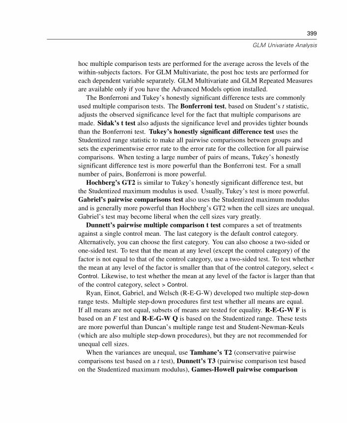
399


hoc multiple comparison tests are performed for the average across the levels of thewithin-subjects factors. For GLM Multivariate, the post hoc tests are performed foreach dependent variable separately. GLM Multivariate and GLM Repeated Measuresare available only if you have the Advanced Models option installed.

The Bonferroni and Tukey’s honestly significant difference tests are commonlyused multiple comparison tests. The Bonferroni test, based on Student’s t statistic,adjusts the observed significance level for the fact that multiple comparisons aremade. Sidak’s t test also adjusts the significance level and provides tighter boundsthan the Bonferroni test. Tukey’s honestly significant difference test uses theStudentized range statistic to make all pairwise comparisons between groups andsets the experimentwise error rate to the error rate for the collection for all pairwisecomparisons. When testing a large number of pairs of means, Tukey’s honestlysignificant difference test is more powerful than the Bonferroni test. For a smallnumber of pairs, Bonferroni is more powerful.

Hochberg’s GT2 is similar to Tukey’s honestly significant difference test, butthe Studentized maximum modulus is used. Usually, Tukey’s test is more powerful.Gabriel’s pairwise comparisons test also uses the Studentized maximum modulusand is generally more powerful than Hochberg’s GT2 when the cell sizes are unequal.Gabriel’s test may become liberal when the cell sizes vary greatly.

Dunnett’s pairwise multiple comparison t test compares a set of treatmentsagainst a single control mean. The last category is the default control category.Alternatively, you can choose the first category. You can also choose a two-sided orone-sided test. To test that the mean at any level (except the control category) of thefactor is not equal to that of the control category, use a two-sided test. To test whetherthe mean at any level of the factor is smaller than that of the control category, select <

Control. Likewise, to test whether the mean at any level of the factor is larger than thatof the control category, select > Control.

Ryan, Einot, Gabriel, and Welsch (R-E-G-W) developed two multiple step-downrange tests. Multiple step-down procedures first test whether all means are equal.If all means are not equal, subsets of means are tested for equality. R-E-G-W F isbased on an F test and R-E-G-W Q is based on the Studentized range. These testsare more powerful than Duncan’s multiple range test and Student-Newman-Keuls(which are also multiple step-down procedures), but they are not recommended forunequal cell sizes.

When the variances are unequal, use Tamhane’s T2 (conservative pairwisecomparisons test based on a t test), Dunnett’s T3 (pairwise comparison test basedon the Studentized maximum modulus), Games-Howell pairwise comparison

400

Chapter 23

test (sometimes liberal), or Dunnett’s C (pairwise comparison test based on theStudentized range).

Duncan’s multiple range test, Student-Newman-Keuls (S-N-K), and Tukey’s bare range tests that rank group means and compute a range value. These tests are notused as frequently as the tests previously discussed.

The Waller-Duncan t test uses a Bayesian approach. This range test uses theharmonic mean of the sample size when the sample sizes are unequal.

The significance level of the Scheffé test is designed to allow all possible linearcombinations of group means to be tested, not just pairwise comparisons available inthis feature. The result is that the Scheffé test is often more conservative than othertests, which means that a larger difference between means is required for significance.

The least significant difference (LSD) pairwise multiple comparison test isequivalent to multiple individual t tests between all pairs of groups. The disadvantageof this test is that no attempt is made to adjust the observed significance level formultiple comparisons.

Tests displayed. Pairwise comparisons are provided for LSD, Sidak, Bonferroni, Gamesand Howell, Tamhane’s T2 and T3, Dunnett’s C, and Dunnett’s T3. Homogeneoussubsets for range tests are provided for S-N-K, Tukey’s b, Duncan, R-E-G-W F,R-E-G-W Q, and Waller. Tukey’s honestly significant difference test, Hochberg’s GT2,Gabriel’s test, and Scheffé’s test are both multiple comparison tests and range tests.

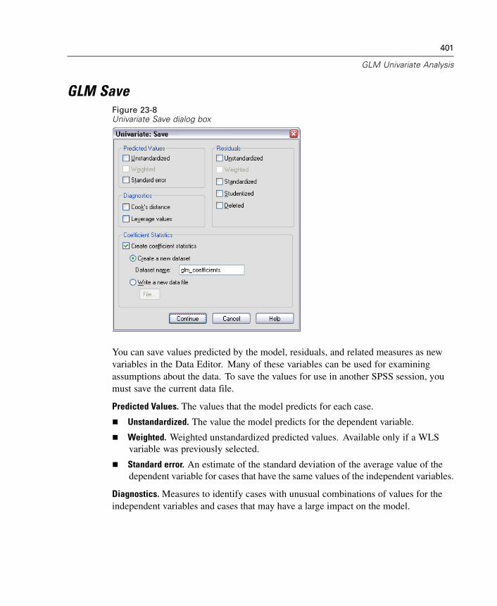
401


GLM SaveFigure 23-8Univariate Save dialog box

You can save values predicted by the model, residuals, and related measures as newvariables in the Data Editor. Many of these variables can be used for examiningassumptions about the data. To save the values for use in another SPSS session, youmust save the current data file.

Predicted Values. The values that the model predicts for each case.

Unstandardized. The value the model predicts for the dependent variable.

Weighted. Weighted unstandardized predicted values. Available only if a WLSvariable was previously selected.

Standard error. An estimate of the standard deviation of the average value of thedependent variable for cases that have the same values of the independent variables.

Diagnostics. Measures to identify cases with unusual combinations of values for theindependent variables and cases that may have a large impact on the model.

402

Chapter 23

Cook's distance. A measure of how much the residuals of all cases would change ifa particular case were excluded from the calculation of the regression coefficients.A large Cook's D indicates that excluding a case from computation of theregression statistics changes the coefficients substantially.

Leverage values. Uncentered leverage values. The relative influence of eachobservation on the model's fit.

Residuals. An unstandardized residual is the actual value of the dependent variableminus the value predicted by the model. Standardized, Studentized, and deletedresiduals are also available. If a WLS variable was chosen, weighted unstandardizedresiduals are available.

Unstandardized. The difference between an observed value and the value predictedby the model.

Weighted. Weighted unstandardized residuals. Available only if a WLS variablewas previously selected.


Studentized. The residual divided by an estimate of its standard deviation thatvaries from case to case, depending on the distance of each case's values on theindependent variables from the means of the independent variables.

Deleted. The residual for a case when that case is excluded from the calculation ofthe regression coefficients. It is the difference between the value of the dependentvariable and the adjusted predicted value.

Coefficient Statistics. Writes a variance-covariance matrix of the parameter estimatesin the model to a new dataset in the current session or an external SPSS-format datafile. Also, for each dependent variable, there will be a row of parameter estimates, arow of significance values for the t statistics corresponding to the parameter estimates,and a row of residual degrees of freedom. For a multivariate model, there are similarrows for each dependent variable. You can use this matrix file in other proceduresthat read an SPSS matrix file.

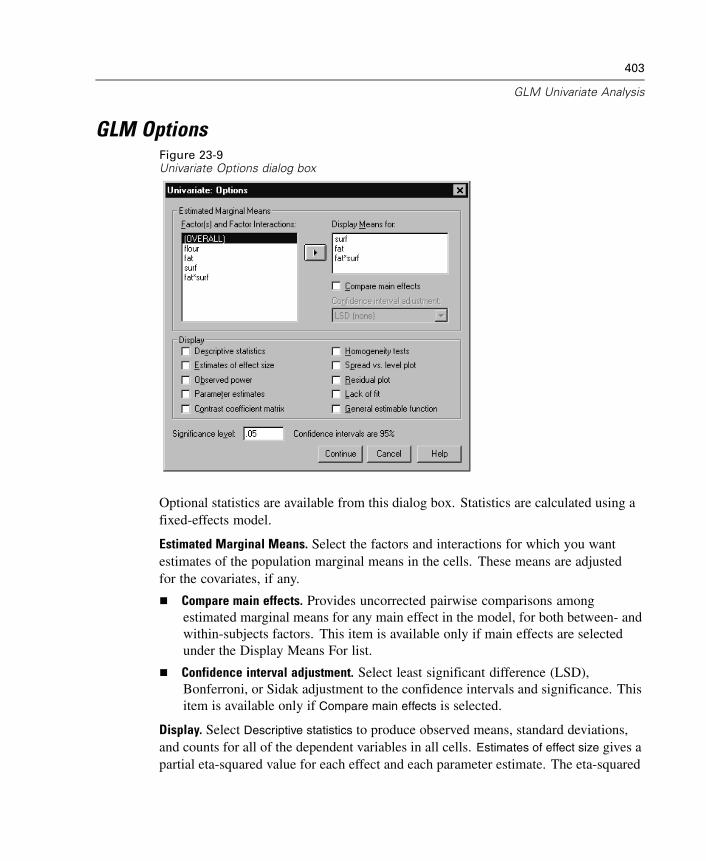
403


GLM OptionsFigure 23-9Univariate Options dialog box

Optional statistics are available from this dialog box. Statistics are calculated using afixed-effects model.

Estimated Marginal Means. Select the factors and interactions for which you wantestimates of the population marginal means in the cells. These means are adjustedfor the covariates, if any.

Compare main effects. Provides uncorrected pairwise comparisons amongestimated marginal means for any main effect in the model, for both between- andwithin-subjects factors. This item is available only if main effects are selectedunder the Display Means For list.

Confidence interval adjustment. Select least significant difference (LSD),Bonferroni, or Sidak adjustment to the confidence intervals and significance. Thisitem is available only if Compare main effects is selected.

Display. Select Descriptive statistics to produce observed means, standard deviations,and counts for all of the dependent variables in all cells. Estimates of effect size gives apartial eta-squared value for each effect and each parameter estimate. The eta-squared

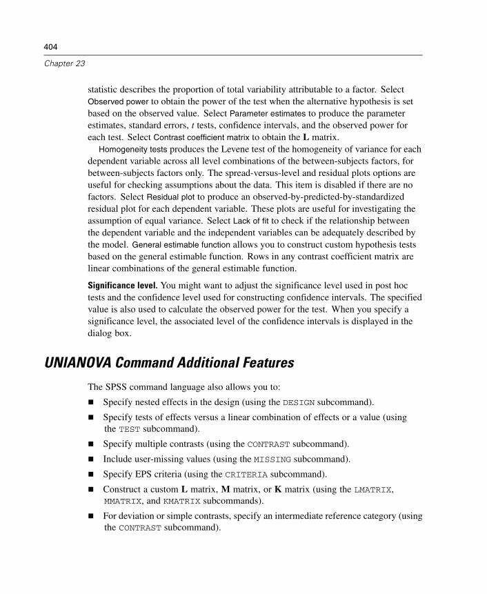
404

Chapter 23

statistic describes the proportion of total variability attributable to a factor. SelectObserved power to obtain the power of the test when the alternative hypothesis is setbased on the observed value. Select Parameter estimates to produce the parameterestimates, standard errors, t tests, confidence intervals, and the observed power foreach test. Select Contrast coefficient matrix to obtain the L matrix.

Homogeneity tests produces the Levene test of the homogeneity of variance for eachdependent variable across all level combinations of the between-subjects factors, forbetween-subjects factors only. The spread-versus-level and residual plots options areuseful for checking assumptions about the data. This item is disabled if there are nofactors. Select Residual plot to produce an observed-by-predicted-by-standardizedresidual plot for each dependent variable. These plots are useful for investigating theassumption of equal variance. Select Lack of fit to check if the relationship betweenthe dependent variable and the independent variables can be adequately described bythe model. General estimable function allows you to construct custom hypothesis testsbased on the general estimable function. Rows in any contrast coefficient matrix arelinear combinations of the general estimable function.

Significance level. You might want to adjust the significance level used in post hoctests and the confidence level used for constructing confidence intervals. The specifiedvalue is also used to calculate the observed power for the test. When you specify asignificance level, the associated level of the confidence intervals is displayed in thedialog box.

UNIANOVA Command Additional Features


Specify nested effects in the design (using the DESIGN subcommand).

Specify tests of effects versus a linear combination of effects or a value (usingthe TEST subcommand).

Specify multiple contrasts (using the CONTRAST subcommand).

Include user-missing values (using the MISSING subcommand).

Specify EPS criteria (using the CRITERIA subcommand).

Construct a custom L matrix, M matrix, or K matrix (using the LMATRIX,MMATRIX, and KMATRIX subcommands).

For deviation or simple contrasts, specify an intermediate reference category (usingthe CONTRAST subcommand).

405


Specify metrics for polynomial contrasts (using the CONTRAST subcommand).

Specify error terms for post hoc comparisons (using the POSTHOC subcommand).

Compute estimated marginal means for any factor or factor interaction among thefactors in the factor list (using the EMMEANS subcommand).

Specify names for temporary variables (using the SAVE subcommand).

Construct a correlation matrix data file (using the OUTFILE subcommand).

Construct a matrix data file that contains statistics from the between-subjectsANOVA table (using the OUTFILE subcommand).

Save the design matrix to a new data file (using the OUTFILE subcommand).


Chapter

24Bivariate Correlations

The Bivariate Correlations procedure computes Pearson’s correlation coefficient,Spearman’s rho, and Kendall’s tau-b with their significance levels. Correlationsmeasure how variables or rank orders are related. Before calculating a correlationcoefficient, screen your data for outliers (which can cause misleading results) andevidence of a linear relationship. Pearson’s correlation coefficient is a measure oflinear association. Two variables can be perfectly related, but if the relationship is notlinear, Pearson’s correlation coefficient is not an appropriate statistic for measuringtheir association.

Example. Is the number of games won by a basketball team correlated with the averagenumber of points scored per game? A scatterplot indicates that there is a linearrelationship. Analyzing data from the 1994–1995 NBA season yields that Pearson’scorrelation coefficient (0.581) is significant at the 0.01 level. You might suspect that themore games won per season, the fewer points the opponents scored. These variablesare negatively correlated (–0.401), and the correlation is significant at the 0.05 level.

Statistics. For each variable: number of cases with nonmissing values, mean, andstandard deviation. For each pair of variables: Pearson’s correlation coefficient,Spearman’s rho, Kendall’s tau-b, cross-product of deviations, and covariance.

Data. Use symmetric quantitative variables for Pearson’s correlation coefficient andquantitative variables or variables with ordered categories for Spearman’s rho andKendall’s tau-b.

Assumptions. Pearson’s correlation coefficient assumes that each pair of variablesis bivariate normal.

407

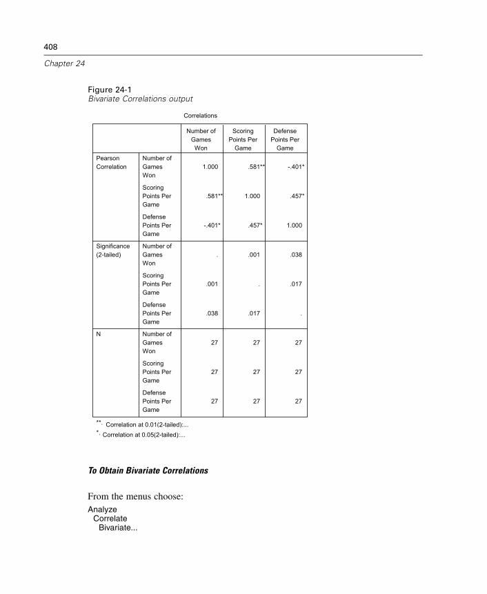
408

Chapter 24

Figure 24-1Bivariate Correlations output

1.000 .581** -.401*

.581** 1.000 .457*

-.401* .457* 1.000

. .001 .038

.001 . .017

.038 .017 .

27 27 27

27 27 27

27 27 27

Number ofGamesWon

ScoringPoints PerGame

DefensePoints PerGame

Number ofGamesWon



Number ofGamesWon



PearsonCorrelation


N

Number ofGames

Won

ScoringPoints Per

Game

DefensePoints Per

Game

Correlations

Correlation at 0.01(2-tailed):...**.

Correlation at 0.05(2-tailed):...*.

To Obtain Bivariate Correlations

From the menus choose:Analyze

CorrelateBivariate...

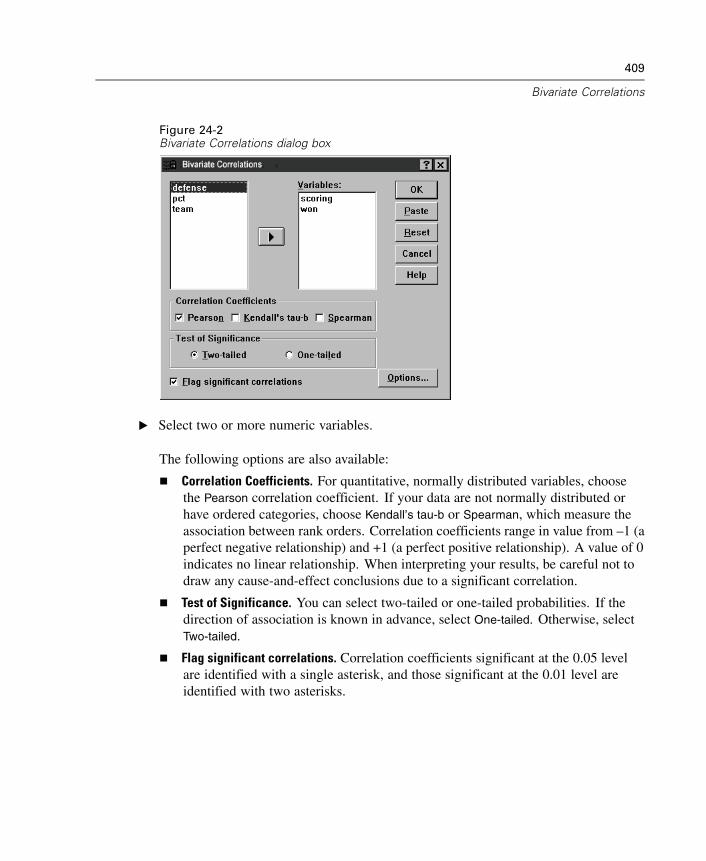
409

Bivariate Correlations

Figure 24-2Bivariate Correlations dialog box

E Select two or more numeric variables.

The following options are also available:

Correlation Coefficients. For quantitative, normally distributed variables, choosethe Pearson correlation coefficient. If your data are not normally distributed orhave ordered categories, choose Kendall’s tau-b or Spearman, which measure theassociation between rank orders. Correlation coefficients range in value from –1 (aperfect negative relationship) and +1 (a perfect positive relationship). A value of 0indicates no linear relationship. When interpreting your results, be careful not todraw any cause-and-effect conclusions due to a significant correlation.

Test of Significance. You can select two-tailed or one-tailed probabilities. If thedirection of association is known in advance, select One-tailed. Otherwise, selectTwo-tailed.

Flag significant correlations. Correlation coefficients significant at the 0.05 levelare identified with a single asterisk, and those significant at the 0.01 level areidentified with two asterisks.

410

Chapter 24

Bivariate Correlations OptionsFigure 24-3Bivariate Correlations Options dialog box

Statistics. For Pearson correlations, you can choose one or both of the following:

Means and standard deviations. Displayed for each variable. The number ofcases with nonmissing values is also shown. Missing values are handled on avariable-by-variable basis regardless of your missing values setting.

Cross-product deviations and covariances. Displayed for each pair of variables. Thecross-product of deviations is equal to the sum of the products of mean-correctedvariables. This is the numerator of the Pearson correlation coefficient. Thecovariance is an unstandardized measure of the relationship between two variables,equal to the cross-product deviation divided by N–1.

Missing Values. You can choose one of the following:

Exclude cases pairwise. Cases with missing values for one or both of a pair ofvariables for a correlation coefficient are excluded from the analysis. Since eachcoefficient is based on all cases that have valid codes on that particular pair ofvariables, the maximum information available is used in every calculation. Thiscan result in a set of coefficients based on a varying number of cases.

Exclude cases listwise. Cases with missing values for any variable are excludedfrom all correlations.

411


CORRELATIONS and NONPAR CORR Command AdditionalFeatures


Write a correlation matrix for Pearson correlations that can be used in placeof raw data to obtain other analyses such as factor analysis (with the MATRIXsubcommand).

Obtain correlations of each variable on a list with each variable on a second list(using the keyword WITH on the VARIABLES subcommand).


Chapter

25Partial Correlations

The Partial Correlations procedure computes partial correlation coefficients thatdescribe the linear relationship between two variables while controlling for the effectsof one or more additional variables. Correlations are measures of linear association.Two variables can be perfectly related, but if the relationship is not linear, a correlationcoefficient is not an appropriate statistic for measuring their association.

Example. Is there a relationship between healthcare funding and disease rates?Although you might expect any such relationship to be a negative one, a study reports asignificant positive correlation: as healthcare funding increases, disease rates appear toincrease. Controlling for the rate of visits to healthcare providers, however, virtuallyeliminates the observed positive correlation. Healthcare funding and disease rates onlyappear to be positively related because more people have access to healthcare whenfunding increases, which leads to more reported diseases by doctors and hospitals.

Statistics. For each variable: number of cases with nonmissing values, mean, andstandard deviation. Partial and zero-order correlation matrices, with degrees offreedom and significance levels.

Data. Use symmetric, quantitative variables.

Assumptions. The Partial Correlations procedure assumes that each pair of variablesis bivariate normal.

413

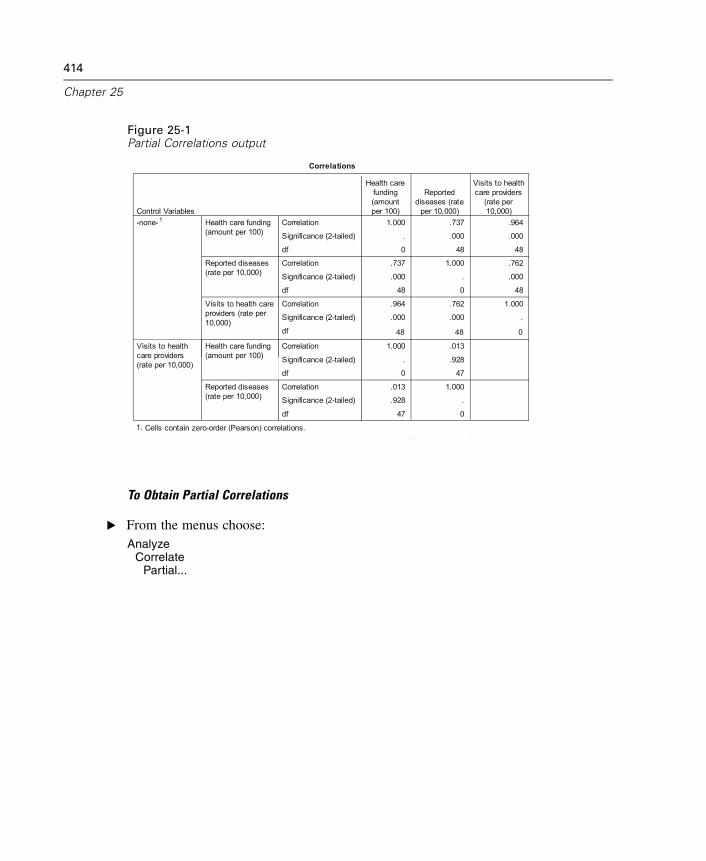
414

Chapter 25

Figure 25-1Partial Correlations output

Correlations

1.000 .737 .964

. .000 .000

0 48 48

.737 1.000 .762

.000 . .000

48 0 48

.964 .762 1.000

.000 .000 .

48 48 0

1.000 .013

. .928

0 47

.013 1.000

.928 .

47 0

Correlation

Significance (2-tailed)

df

Correlation


df

Correlation


df

Correlation


df

Correlation


df

Health care funding(amount per 100)

Reported diseases(rate per 10,000)

Visits to health careproviders (rate per10,000)

Health care funding(amount per 100)

Reported diseases(rate per 10,000)

Control Variables-none-1

Visits to healthcare providers(rate per 10,000)

Health carefunding(amountper 100)

Reporteddiseases (rate

per 10,000)

Visits to healthcare providers

(rate per10,000)

Cells contain zero-order (Pearson) correlations.1.

To Obtain Partial Correlations


CorrelatePartial...

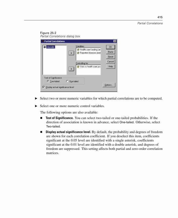
415

Partial Correlations

Figure 25-2Partial Correlations dialog box

E Select two or more numeric variables for which partial correlations are to be computed.

E Select one or more numeric control variables.


Test of Significance. You can select two-tailed or one-tailed probabilities. If thedirection of association is known in advance, select One-tailed. Otherwise, selectTwo-tailed.

Display actual significance level. By default, the probability and degrees of freedomare shown for each correlation coefficient. If you deselect this item, coefficientssignificant at the 0.05 level are identified with a single asterisk, coefficientssignificant at the 0.01 level are identified with a double asterisk, and degrees offreedom are suppressed. This setting affects both partial and zero-order correlationmatrices.

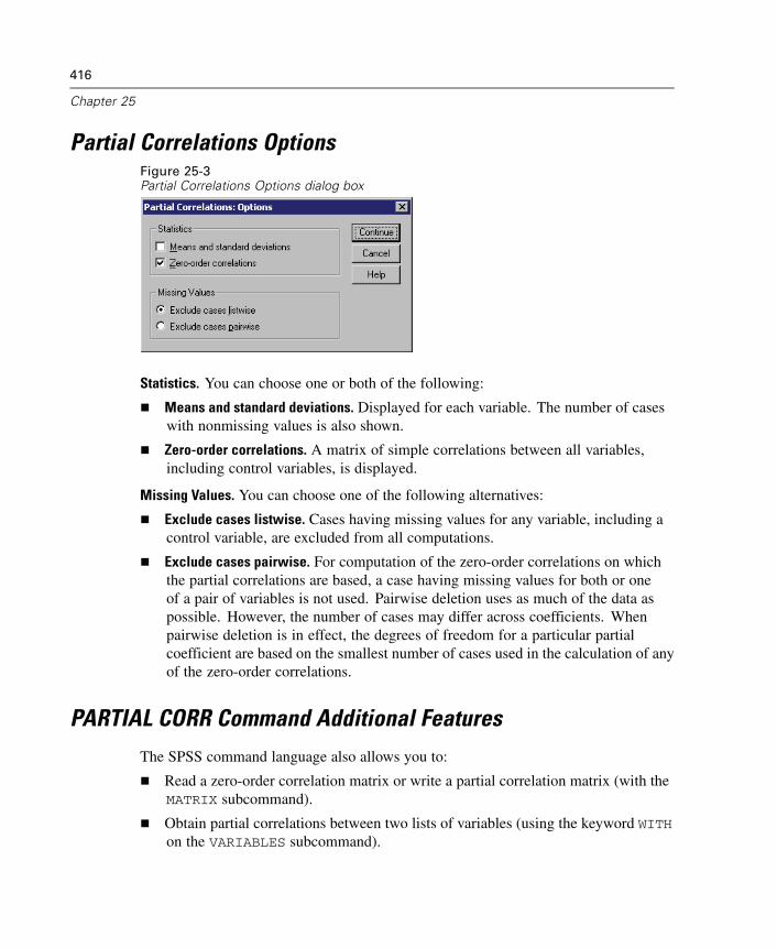
416

Chapter 25

Partial Correlations OptionsFigure 25-3Partial Correlations Options dialog box

Statistics. You can choose one or both of the following:

Means and standard deviations. Displayed for each variable. The number of caseswith nonmissing values is also shown.

Zero-order correlations. A matrix of simple correlations between all variables,including control variables, is displayed.

Missing Values. You can choose one of the following alternatives:

Exclude cases listwise. Cases having missing values for any variable, including acontrol variable, are excluded from all computations.

Exclude cases pairwise. For computation of the zero-order correlations on whichthe partial correlations are based, a case having missing values for both or oneof a pair of variables is not used. Pairwise deletion uses as much of the data aspossible. However, the number of cases may differ across coefficients. Whenpairwise deletion is in effect, the degrees of freedom for a particular partialcoefficient are based on the smallest number of cases used in the calculation of anyof the zero-order correlations.

PARTIAL CORR Command Additional FeaturesThe SPSS command language also allows you to:

Read a zero-order correlation matrix or write a partial correlation matrix (with theMATRIX subcommand).

Obtain partial correlations between two lists of variables (using the keyword WITHon the VARIABLES subcommand).

417

Partial Correlations

Obtain multiple analyses (with multiple VARIABLES subcommands).

Specify order values to request (for example, both first- and second-orderpartial correlations) when you have two control variables (with the VARIABLESsubcommand).

Suppress redundant coefficients (with the FORMAT subcommand).

Display a matrix of simple correlations when some coefficients cannot becomputed (with the STATISTICS subcommand).


Chapter

26Distances

This procedure calculates any of a wide variety of statistics measuring eithersimilarities or dissimilarities (distances), either between pairs of variables or betweenpairs of cases. These similarity or distance measures can then be used with otherprocedures, such as factor analysis, cluster analysis, or multidimensional scaling, tohelp analyze complex datasets.

Example. Is it possible to measure similarities between pairs of automobiles based oncertain characteristics, such as engine size, MPG, and horsepower? By computingsimilarities between autos, you can gain a sense of which autos are similar to eachother and which are different from each other. For a more formal analysis, you mightconsider applying a hierarchical cluster analysis or multidimensional scaling to thesimilarities to explore the underlying structure.

Statistics. Dissimilarity (distance) measures for interval data are Euclidean distance,squared Euclidean distance, Chebychev, block, Minkowski, or customized; for countdata, chi-square or phi-square; for binary data, Euclidean distance, squared Euclideandistance, size difference, pattern difference, variance, shape, or Lance and Williams.Similarity measures for interval data are Pearson correlation or cosine; for binarydata, Russel and Rao, simple matching, Jaccard, dice, Rogers and Tanimoto, Sokaland Sneath 1, Sokal and Sneath 2, Sokal and Sneath 3, Kulczynski 1, Kulczynski 2,Sokal and Sneath 4, Hamann, Lambda, Anderberg’s D, Yule’s Y, Yule’s Q, Ochiai,Sokal and Sneath 5, phi 4-point correlation, or dispersion.

To Obtain Distance Matrices


CorrelateDistances...

419

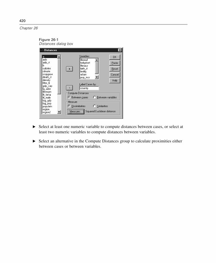
420

Chapter 26

Figure 26-1Distances dialog box

E Select at least one numeric variable to compute distances between cases, or select atleast two numeric variables to compute distances between variables.

E Select an alternative in the Compute Distances group to calculate proximities eitherbetween cases or between variables.

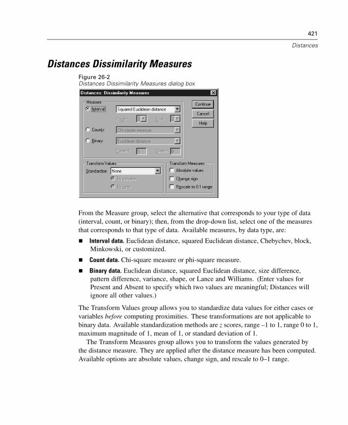
421

Distances

Distances Dissimilarity MeasuresFigure 26-2Distances Dissimilarity Measures dialog box

From the Measure group, select the alternative that corresponds to your type of data(interval, count, or binary); then, from the drop-down list, select one of the measuresthat corresponds to that type of data. Available measures, by data type, are:

Interval data. Euclidean distance, squared Euclidean distance, Chebychev, block,Minkowski, or customized.

Count data. Chi-square measure or phi-square measure.

Binary data. Euclidean distance, squared Euclidean distance, size difference,pattern difference, variance, shape, or Lance and Williams. (Enter values forPresent and Absent to specify which two values are meaningful; Distances willignore all other values.)

The Transform Values group allows you to standardize data values for either cases orvariables before computing proximities. These transformations are not applicable tobinary data. Available standardization methods are z scores, range –1 to 1, range 0 to 1,maximum magnitude of 1, mean of 1, or standard deviation of 1.

The Transform Measures group allows you to transform the values generated bythe distance measure. They are applied after the distance measure has been computed.Available options are absolute values, change sign, and rescale to 0–1 range.

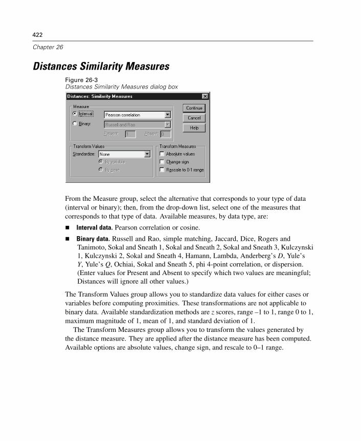
422

Chapter 26

Distances Similarity MeasuresFigure 26-3Distances Similarity Measures dialog box

From the Measure group, select the alternative that corresponds to your type of data(interval or binary); then, from the drop-down list, select one of the measures thatcorresponds to that type of data. Available measures, by data type, are:

Interval data. Pearson correlation or cosine.

Binary data. Russell and Rao, simple matching, Jaccard, Dice, Rogers andTanimoto, Sokal and Sneath 1, Sokal and Sneath 2, Sokal and Sneath 3, Kulczynski1, Kulczynski 2, Sokal and Sneath 4, Hamann, Lambda, Anderberg’s D, Yule’sY, Yule’s Q, Ochiai, Sokal and Sneath 5, phi 4-point correlation, or dispersion.(Enter values for Present and Absent to specify which two values are meaningful;Distances will ignore all other values.)

The Transform Values group allows you to standardize data values for either cases orvariables before computing proximities. These transformations are not applicable tobinary data. Available standardization methods are z scores, range –1 to 1, range 0 to 1,maximum magnitude of 1, mean of 1, and standard deviation of 1.

The Transform Measures group allows you to transform the values generated bythe distance measure. They are applied after the distance measure has been computed.Available options are absolute values, change sign, and rescale to 0–1 range.

423

Distances

PROXIMITIES Command Additional Features

The Distances procedure uses PROXIMITIES command syntax. The SPSS commandlanguage also allows you to:

Specify any integer as the power for the Minkowski distance measure.

Specify any integers as the power and root for a customized distance measure.


Chapter

27Linear Regression

Linear Regression estimates the coefficients of the linear equation, involving one ormore independent variables, that best predict the value of the dependent variable.For example, you can try to predict a salesperson’s total yearly sales (the dependentvariable) from independent variables such as age, education, and years of experience.

Example. Is the number of games won by a basketball team in a season related to theaverage number of points the team scores per game? A scatterplot indicates that thesevariables are linearly related. The number of games won and the average numberof points scored by the opponent are also linearly related. These variables have anegative relationship. As the number of games won increases, the average numberof points scored by the opponent decreases. With linear regression, you can modelthe relationship of these variables. A good model can be used to predict how manygames teams will win.

Statistics. For each variable: number of valid cases, mean, and standard deviation.For each model: regression coefficients, correlation matrix, part and partialcorrelations, multiple R, R2, adjusted R2, change in R2, standard error of the estimate,analysis-of-variance table, predicted values, and residuals. Also, 95%-confidenceintervals for each regression coefficient, variance-covariance matrix, variance inflationfactor, tolerance, Durbin-Watson test, distance measures (Mahalanobis, Cook, andleverage values), DfBeta, DfFit, prediction intervals, and casewise diagnostics. Plots:scatterplots, partial plots, histograms, and normal probability plots.

Data. The dependent and independent variables should be quantitative. Categoricalvariables, such as religion, major field of study, or region of residence, need to berecoded to binary (dummy) variables or other types of contrast variables.

Assumptions. For each value of the independent variable, the distribution of thedependent variable must be normal. The variance of the distribution of the dependentvariable should be constant for all values of the independent variable. The relationship

425

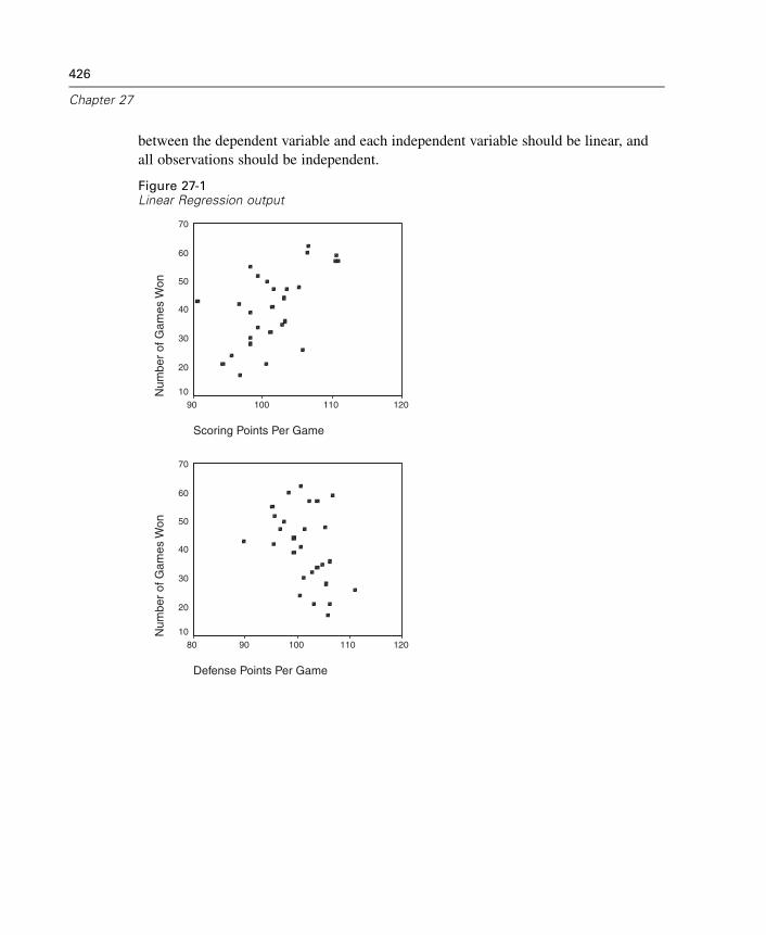
426

Chapter 27

between the dependent variable and each independent variable should be linear, andall observations should be independent.

Figure 27-1Linear Regression output

Scoring Points Per Game

12011010090

Num

ber

of G

ames

Won

70

60

50

40

30

20

10

Defense Points Per Game

1201101009080

Num

ber

of G

ames

Won

70

60

50

40

30

20

10

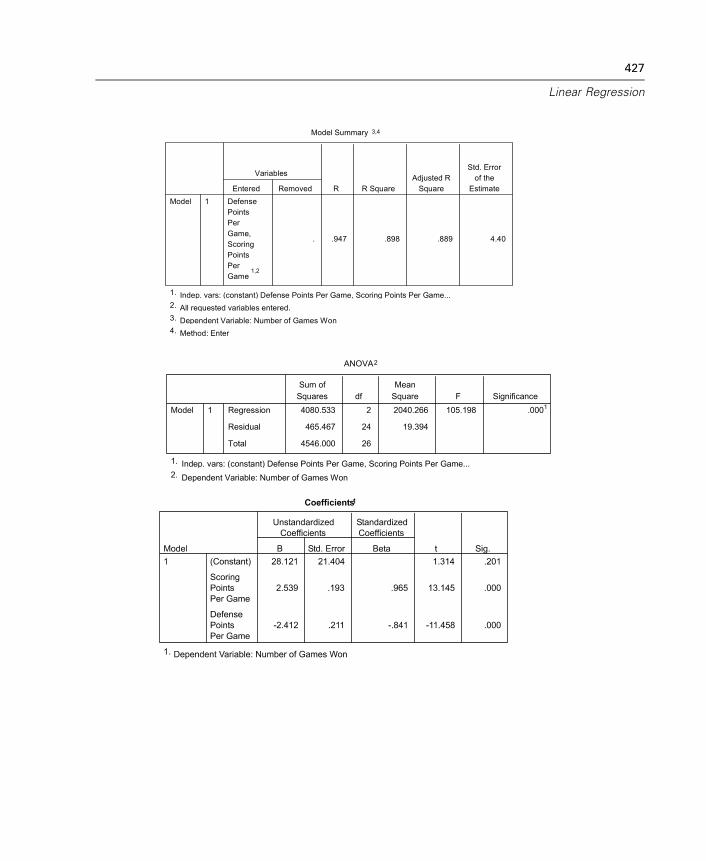
427

Linear Regression

DefensePointsPerGame,ScoringPointsPerGame

1,2

. .947 .898 .889 4.40

1ModelEntered Removed

Variables

R R SquareAdjusted R

Square

Std. Errorof the

Estimate

Model Summary 3,4

Indep. vars: (constant) Defense Points Per Game, Scoring Points Per Game...1.

All requested variables entered.2.

Dependent Variable: Number of Games Won3.

Method: Enter4.

4080.533 2 2040.266 105.198 .0001

465.467 24 19.394

4546.000 26

Regression

Residual

Total

1Model

Sum ofSquares df

MeanSquare F Significance

ANOVA2

Indep. vars: (constant) Defense Points Per Game, Scoring Points Per Game...1.

Dependent Variable: Number of Games Won2.

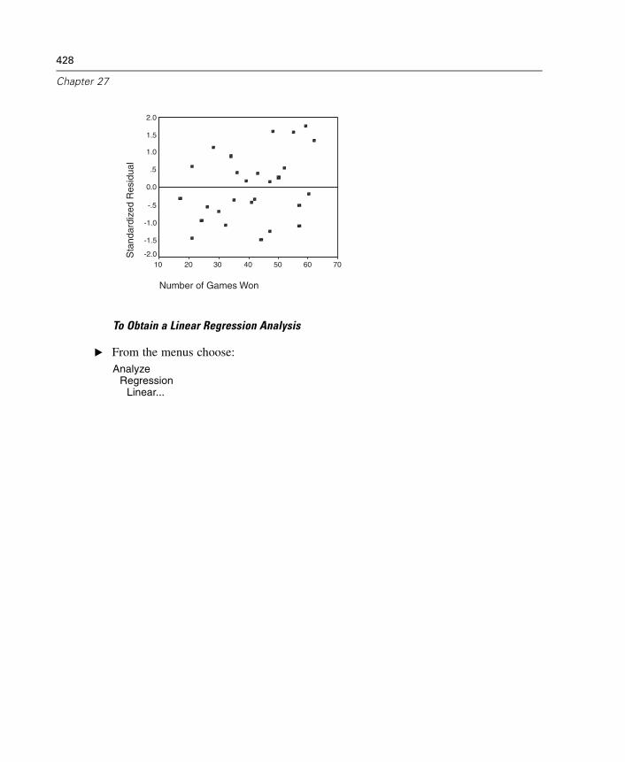
428

Chapter 27

Number of Games Won

70605040302010

Sta

ndar

dize

d R

esid

ual

2.0

1.5

1.0

.5

0.0

-.5

-1.0

-1.5

-2.0

To Obtain a Linear Regression Analysis


RegressionLinear...

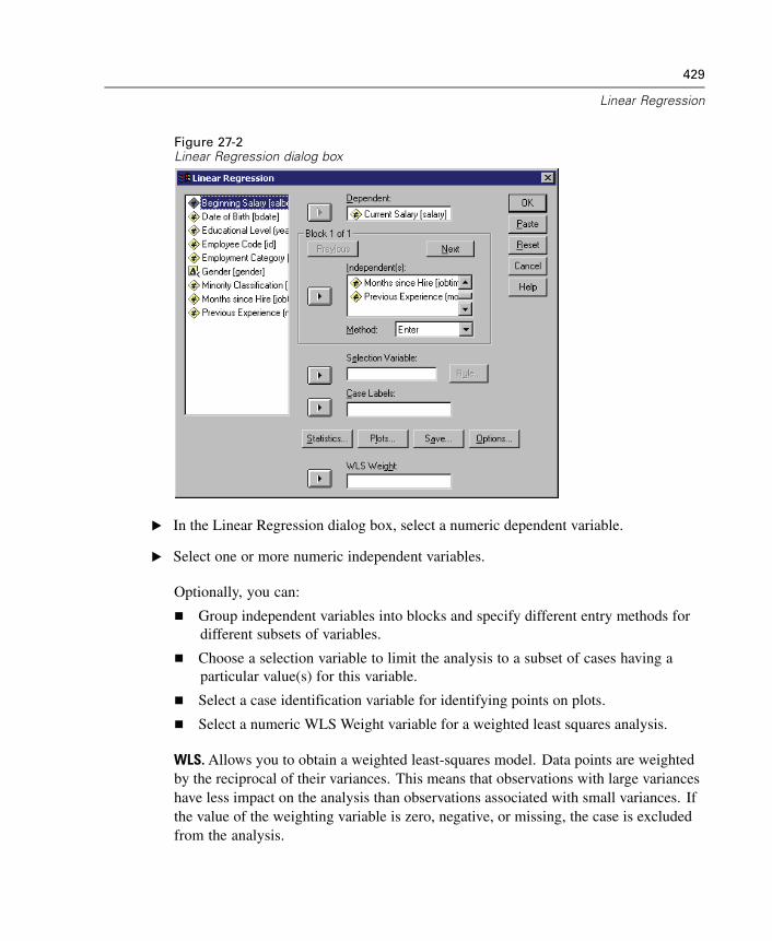
429

Linear Regression

Figure 27-2Linear Regression dialog box

E In the Linear Regression dialog box, select a numeric dependent variable.

E Select one or more numeric independent variables.


Group independent variables into blocks and specify different entry methods fordifferent subsets of variables.

Choose a selection variable to limit the analysis to a subset of cases having aparticular value(s) for this variable.

Select a case identification variable for identifying points on plots.

Select a numeric WLS Weight variable for a weighted least squares analysis.

WLS. Allows you to obtain a weighted least-squares model. Data points are weightedby the reciprocal of their variances. This means that observations with large varianceshave less impact on the analysis than observations associated with small variances. Ifthe value of the weighting variable is zero, negative, or missing, the case is excludedfrom the analysis.

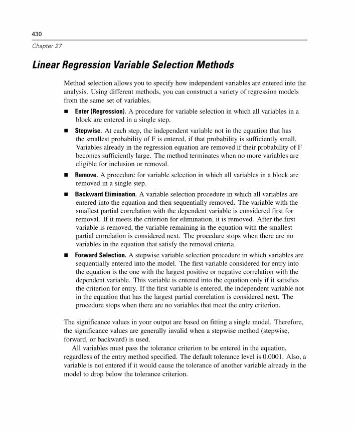
430

Chapter 27

Linear Regression Variable Selection Methods

Method selection allows you to specify how independent variables are entered into theanalysis. Using different methods, you can construct a variety of regression modelsfrom the same set of variables.

Enter (Regression). A procedure for variable selection in which all variables in ablock are entered in a single step.

Stepwise. At each step, the independent variable not in the equation that hasthe smallest probability of F is entered, if that probability is sufficiently small.Variables already in the regression equation are removed if their probability of Fbecomes sufficiently large. The method terminates when no more variables areeligible for inclusion or removal.

Remove. A procedure for variable selection in which all variables in a block areremoved in a single step.

Backward Elimination. A variable selection procedure in which all variables areentered into the equation and then sequentially removed. The variable with thesmallest partial correlation with the dependent variable is considered first forremoval. If it meets the criterion for elimination, it is removed. After the firstvariable is removed, the variable remaining in the equation with the smallestpartial correlation is considered next. The procedure stops when there are novariables in the equation that satisfy the removal criteria.

Forward Selection. A stepwise variable selection procedure in which variables aresequentially entered into the model. The first variable considered for entry intothe equation is the one with the largest positive or negative correlation with thedependent variable. This variable is entered into the equation only if it satisfiesthe criterion for entry. If the first variable is entered, the independent variable notin the equation that has the largest partial correlation is considered next. Theprocedure stops when there are no variables that meet the entry criterion.

The significance values in your output are based on fitting a single model. Therefore,the significance values are generally invalid when a stepwise method (stepwise,forward, or backward) is used.

All variables must pass the tolerance criterion to be entered in the equation,regardless of the entry method specified. The default tolerance level is 0.0001. Also, avariable is not entered if it would cause the tolerance of another variable already in themodel to drop below the tolerance criterion.

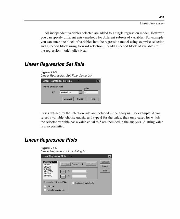
431

Linear Regression

All independent variables selected are added to a single regression model. However,you can specify different entry methods for different subsets of variables. For example,you can enter one block of variables into the regression model using stepwise selectionand a second block using forward selection. To add a second block of variables tothe regression model, click Next.

Linear Regression Set RuleFigure 27-3Linear Regression Set Rule dialog box

Cases defined by the selection rule are included in the analysis. For example, if youselect a variable, choose equals, and type 5 for the value, then only cases for whichthe selected variable has a value equal to 5 are included in the analysis. A string valueis also permitted.

Linear Regression PlotsFigure 27-4Linear Regression Plots dialog box

432

Chapter 27

Plots can aid in the validation of the assumptions of normality, linearity, and equalityof variances. Plots are also useful for detecting outliers, unusual observations, andinfluential cases. After saving them as new variables, predicted values, residuals,and other diagnostics are available in the Data Editor for constructing plots with theindependent variables. The following plots are available:

Scatterplots. You can plot any two of the following: the dependent variable,standardized predicted values, standardized residuals, deleted residuals, adjustedpredicted values, Studentized residuals, or Studentized deleted residuals. Plot thestandardized residuals against the standardized predicted values to check for linearityand equality of variances.

Source variable list. Lists the dependent variable (DEPENDNT) and the followingpredicted and residual variables: Standardized predicted values (*ZPRED),Standardized residuals (*ZRESID), Deleted residuals (*DRESID), Adjusted predictedvalues (*ADJPRED), Studentized residuals (*SRESID), Studentized deleted residuals(*SDRESID).

Produce all partial plots. Displays scatterplots of residuals of each independentvariable and the residuals of the dependent variable when both variables are regressedseparately on the rest of the independent variables. At least two independent variablesmust be in the equation for a partial plot to be produced.

Standardized Residual Plots. You can obtain histograms of standardized residuals andnormal probability plots comparing the distribution of standardized residuals to anormal distribution.

If any plots are requested, summary statistics are displayed for standardized predictedvalues and standardized residuals (*ZPRED and *ZRESID).

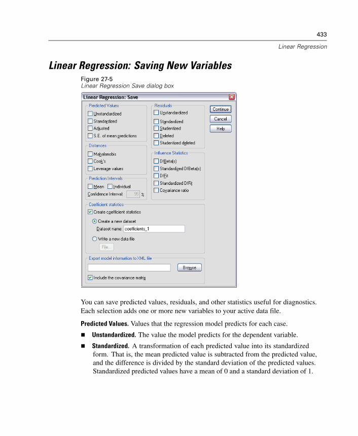
433

Linear Regression

Linear Regression: Saving New VariablesFigure 27-5Linear Regression Save dialog box

You can save predicted values, residuals, and other statistics useful for diagnostics.Each selection adds one or more new variables to your active data file.

Predicted Values. Values that the regression model predicts for each case.

Unstandardized. The value the model predicts for the dependent variable.

Standardized. A transformation of each predicted value into its standardizedform. That is, the mean predicted value is subtracted from the predicted value,and the difference is divided by the standard deviation of the predicted values.Standardized predicted values have a mean of 0 and a standard deviation of 1.

434

Chapter 27

Adjusted. The predicted value for a case when that case is excluded from thecalculation of the regression coefficients.

S.E. of mean predictions. Standard errors of the predicted values. An estimate of thestandard deviation of the average value of the dependent variable for cases thathave the same values of the independent variables.

Distances. Measures to identify cases with unusual combinations of values for theindependent variables and cases that may have a large impact on the regression model.

Mahalanobis. A measure of how much a case's values on the independent variablesdiffer from the average of all cases. A large Mahalanobis distance identifies a caseas having extreme values on one or more of the independent variables.

Cook's. A measure of how much the residuals of all cases would change if aparticular case were excluded from the calculation of the regression coefficients. Alarge Cook's D indicates that excluding a case from computation of the regressionstatistics changes the coefficients substantially.

Leverage values. Measures the influence of a point on the fit of the regression. Thecentered leverage ranges from 0 (no influence on the fit) to (N-1)/N.

Prediction Intervals. The upper and lower bounds for both mean and individualprediction intervals.

Mean. Lower and upper bounds (two variables) for the prediction interval of themean predicted response.

Individual. Lower and upper bounds (two variables) for the prediction interval ofthe dependent variable for a single case.

Confidence Interval. Enter a value between 1 and 99.99 to specify the confidencelevel for the two Prediction Intervals. Mean or Individual must be selected beforeentering this value. Typical confidence interval values are 90, 95, and 99.

Residuals. The actual value of the dependent variable minus the value predicted bythe regression equation.

Unstandardized. The difference between an observed value and the value predictedby the model.


435

Linear Regression

Studentized. The residual divided by an estimate of its standard deviation thatvaries from case to case, depending on the distance of each case's values on theindependent variables from the means of the independent variables.

Deleted. The residual for a case when that case is excluded from the calculation ofthe regression coefficients. It is the difference between the value of the dependentvariable and the adjusted predicted value.

Studentized deleted. The deleted residual for a case divided by its standarderror. The difference between a Studentized deleted residual and its associatedStudentized residual indicates how much difference eliminating a case makeson its own prediction.

Influence Statistics. The change in the regression coefficients (DfBeta[s]) and predictedvalues (DfFit) that results from the exclusion of a particular case. StandardizedDfBetas and DfFit values are also available along with the covariance ratio.

DfBeta(s). The difference in beta value is the change in the regression coefficientthat results from the exclusion of a particular case. A value is computed for eachterm in the model, including the constant.

Standardized DfBeta. Standardized difference in beta value. The change in theregression coefficient that results from the exclusion of a particular case. You maywant to examine cases with absolute values greater than 2 divided by the squareroot of N, where N is the number of cases. A value is computed for each termin the model, including the constant.

DfFit. The difference in fit value is the change in the predicted value that resultsfrom the exclusion of a particular case.

Standardized DfFit. Standardized difference in fit value. The change in the predictedvalue that results from the exclusion of a particular case. You may want to examinestandardized values which in absolute value exceed 2 times the square root of p/N,where p is the number of parameters in the model and N is the number of cases.

Covariance ratio. The ratio of the determinant of the covariance matrix with aparticular case excluded from the calculation of the regression coefficients to thedeterminant of the covariance matrix with all cases included. If the ratio is close to1, the case does not significantly alter the covariance matrix.

Coefficient Statistics. Saves regression coefficients to a dataset or a data file. Datasetsare available for subsequent use in the same session but are not saved as files unlessexplicitly saved prior to the end of the session. Dataset names must conform to SPSS

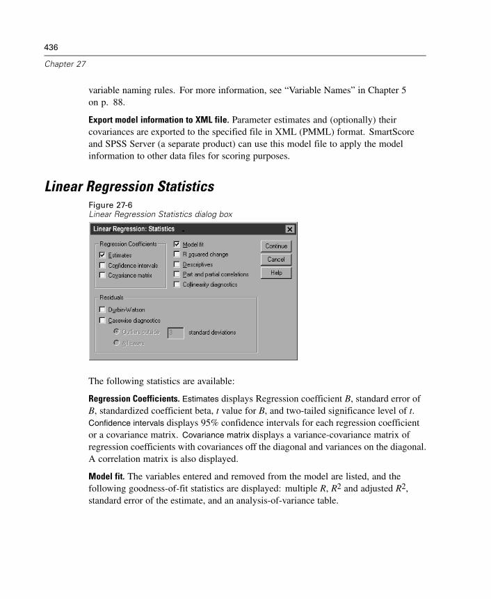
436

Chapter 27

variable naming rules. For more information, see “Variable Names” in Chapter 5on p. 88.

Export model information to XML file. Parameter estimates and (optionally) theircovariances are exported to the specified file in XML (PMML) format. SmartScoreand SPSS Server (a separate product) can use this model file to apply the modelinformation to other data files for scoring purposes.

Linear Regression StatisticsFigure 27-6Linear Regression Statistics dialog box

The following statistics are available:

Regression Coefficients. Estimates displays Regression coefficient B, standard error ofB, standardized coefficient beta, t value for B, and two-tailed significance level of t.Confidence intervals displays 95% confidence intervals for each regression coefficientor a covariance matrix. Covariance matrix displays a variance-covariance matrix ofregression coefficients with covariances off the diagonal and variances on the diagonal.A correlation matrix is also displayed.

Model fit. The variables entered and removed from the model are listed, and thefollowing goodness-of-fit statistics are displayed: multiple R, R2 and adjusted R2,standard error of the estimate, and an analysis-of-variance table.

437

Linear Regression

R squared change. The change in the R2 statistic that is produced by adding or deletingan independent variable. If the R2 change associated with a variable is large, thatmeans that the variable is a good predictor of the dependent variable.

Descriptives. Provides the number of valid cases, the mean, and the standard deviationfor each variable in the analysis. A correlation matrix with a one-tailed significancelevel and the number of cases for each correlation are also displayed.

Partial Correlation. The correlation that remains between two variables after removingthe correlation that is due to their mutual association with the other variables. Thecorrelation between the dependent variable and an independent variable when the lineareffects of the other independent variables in the model have been removed from both.

Part Correlation. The correlation between the dependent variable and an independentvariable when the linear effects of the other independent variables in the model havebeen removed from the independent variable. It is related to the change in R squaredwhen a variable is added to an equation. Sometimes called the semipartial correlation.

Collinearity diagnostics. Collinearity (or multicollinearity) is the undesirable situationwhen one independent variable is a linear function of other independent variables.Eigenvalues of the scaled and uncentered cross-products matrix, condition indices, andvariance-decomposition proportions are displayed along with variance inflation factors(VIF) and tolerances for individual variables.

Residuals. Displays the Durbin-Watson test for serial correlation of the residuals andcasewise diagnostics for the cases meeting the selection criterion (outliers aboven standard deviations).

438

Chapter 27

Linear Regression OptionsFigure 27-7Linear Regression Options dialog box

The following options are available:

Stepping Method Criteria. These options apply when either the forward, backward, orstepwise variable selection method has been specified. Variables can be entered orremoved from the model depending on either the significance (probability) of the Fvalue or the F value itself.

Use Probability of F. A variable is entered into the model if the significance level ofits F value is less than the Entry value and is removed if the significance level isgreater than the Removal value. Entry must be less than Removal, and both valuesmust be positive. To enter more variables into the model, increase the Entry value.To remove more variables from the model, lower the Removal value.

Use F Value. A variable is entered into the model if its F value is greater than theEntry value and is removed if the F value is less than the Removal value. Entrymust be greater than Removal, and both values must be positive. To enter morevariables into the model, lower the Entry value. To remove more variables fromthe model, increase the Removal value.

Include constant in equation. By default, the regression model includes a constant term.Deselecting this option forces regression through the origin, which is rarely done.Some results of regression through the origin are not comparable to results of regressionthat do include a constant. For example, R2 cannot be interpreted in the usual way.

439

Linear Regression

Missing Values. You can choose one of the following:

Exclude cases listwise. Only cases with valid values for all variables are includedin the analyses.

Exclude cases pairwise. Cases with complete data for the pair of variables beingcorrelated are used to compute the correlation coefficient on which the regressionanalysis is based. Degrees of freedom are based on the minimum pairwise N.

Replace with mean. All cases are used for computations, with the mean of thevariable substituted for missing observations.

REGRESSION Command Additional Features


Write a correlation matrix or read a matrix in place of raw data to obtain yourregression analysis (with the MATRIX subcommand).

Specify tolerance levels (with the CRITERIA subcommand).

Obtain multiple models for the same or different dependent variables (with theMETHOD and DEPENDENT subcommands).

Obtain additional statistics (with the DESCRIPTIVES and STATISTICSsubcommands).


Chapter

28Curve Estimation

The Curve Estimation procedure produces curve estimation regression statistics andrelated plots for 11 different curve estimation regression models. A separate model isproduced for each dependent variable. You can also save predicted values, residuals,and prediction intervals as new variables.

Example. An Internet service provider tracks the percentage of virus-infected e-mailtraffic on its networks over time. A scatterplot reveals that the relationship is nonlinear.You might fit a quadratic or cubic model to the data and check the validity ofassumptions and the goodness of fit of the model.

Statistics. For each model: regression coefficients, multiple R, R2, adjusted R2,standard error of the estimate, analysis-of-variance table, predicted values, residuals,and prediction intervals. Models: linear, logarithmic, inverse, quadratic, cubic, power,compound, S-curve, logistic, growth, and exponential.

Data. The dependent and independent variables should be quantitative. If you selectTime from the active dataset as the independent variable (instead of selecting avariable), the Curve Estimation procedure generates a time variable where the lengthof time between cases is uniform. If Time is selected, the dependent variable shouldbe a time-series measure. Time-series analysis requires a data file structure in whicheach case (row) represents a set of observations at a different time and the length oftime between cases is uniform.

Assumptions. Screen your data graphically to determine how the independent anddependent variables are related (linearly, exponentially, etc.). The residuals of a goodmodel should be randomly distributed and normal. If a linear model is used, thefollowing assumptions should be met: For each value of the independent variable, thedistribution of the dependent variable must be normal. The variance of the distributionof the dependent variable should be constant for all values of the independent variable.The relationship between the dependent variable and the independent variable shouldbe linear, and all observations should be independent.

441

442

Chapter 28

Figure 28-1Curve Estimation summary table

Figure 28-2Curve Estimation ANOVA

Figure 28-3Curve Estimation coefficients

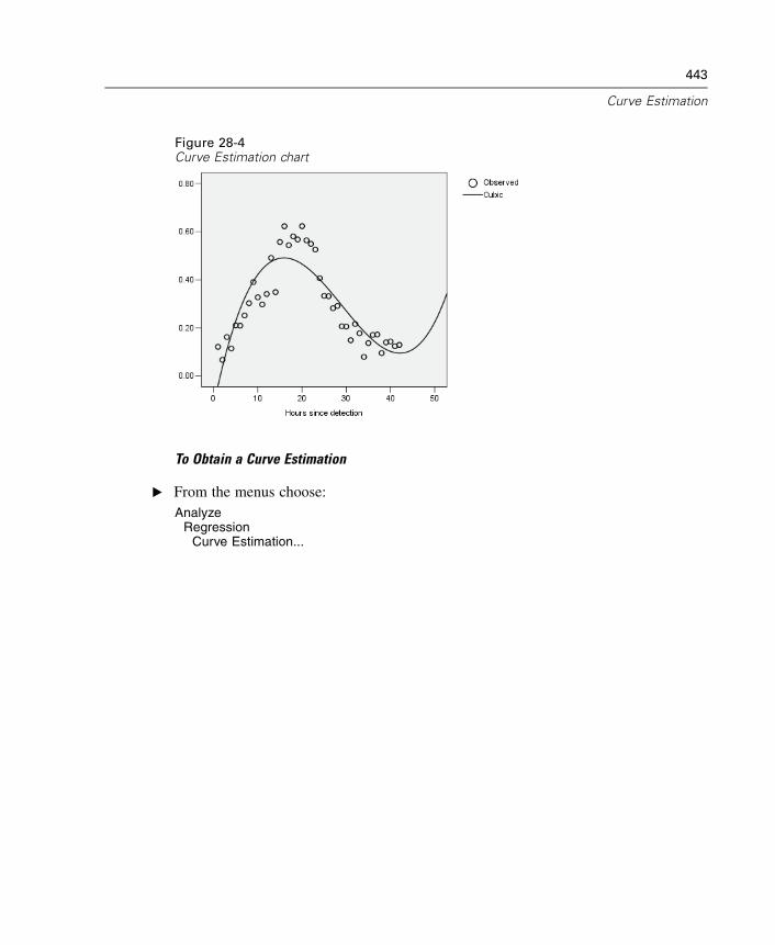
443

Curve Estimation

Figure 28-4Curve Estimation chart

To Obtain a Curve Estimation


RegressionCurve Estimation...

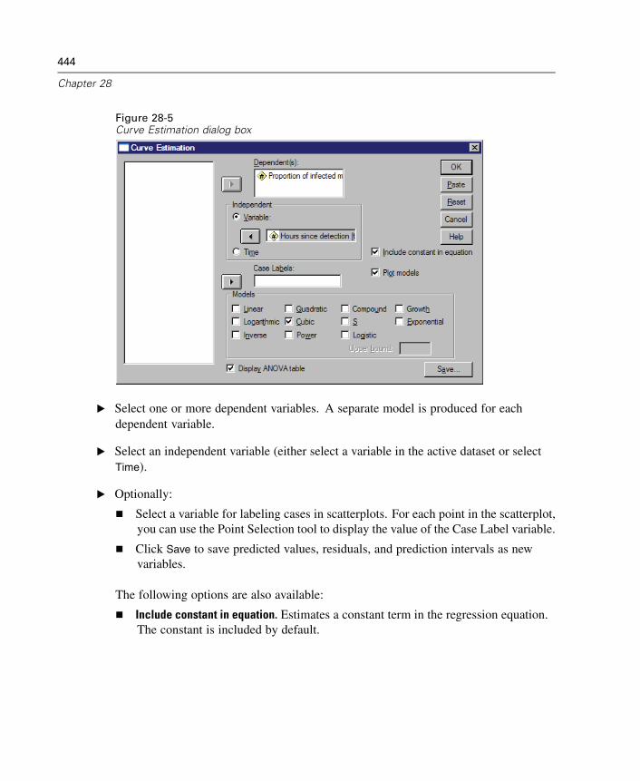
444

Chapter 28

Figure 28-5Curve Estimation dialog box

E Select one or more dependent variables. A separate model is produced for eachdependent variable.

E Select an independent variable (either select a variable in the active dataset or selectTime).

E Optionally:

Select a variable for labeling cases in scatterplots. For each point in the scatterplot,you can use the Point Selection tool to display the value of the Case Label variable.

Click Save to save predicted values, residuals, and prediction intervals as newvariables.


Include constant in equation. Estimates a constant term in the regression equation.The constant is included by default.

445

Curve Estimation

Plot models. Plots the values of the dependent variable and each selected modelagainst the independent variable. A separate chart is produced for each dependentvariable.

Display ANOVA table. Displays a summary analysis-of-variance table for eachselected model.

Curve Estimation ModelsYou can choose one or more curve estimation regression models. To determine whichmodel to use, plot your data. If your variables appear to be related linearly, use a simplelinear regression model. When your variables are not linearly related, try transformingyour data. When a transformation does not help, you may need a more complicatedmodel. View a scatterplot of your data; if the plot resembles a mathematical functionyou recognize, fit your data to that type of model. For example, if your data resemblean exponential function, use an exponential model.

Linear. Model whose equation is Y = b0 + (b1 * t). The series values are modeled as alinear function of time.

Logarithmic. Model whose equation is Y = b0 + (b1 * ln(t)).

Inverse. Model whose equation is Y = b0 + (b1 / t).

Quadratic. Model whose equation is Y = b0 + (b1 * t) + (b2 * t**2). The quadraticmodel can be used to model a series that "takes off" or a series that dampens.

Cubic. Model that is defined by the equation Y = b0 + (b1 * t) + (b2 * t**2) + (b3* t**3).

Power. Model whose equation is Y = b0 * (t**b1) or ln(Y) = ln(b0) + (b1 * ln(t)).

Compound. Model whose equation is Y = b0 * (b1**t) or ln(Y) = ln(b0) + (ln(b1) * t).

S-curve. Model whose equation is Y = e**(b0 + (b1/t)) or ln(Y) = b0 + (b1/t).

Logistic. Model whose equation is Y = 1 / (1/u + (b0 * (b1**t))) or ln(1/y-1/u) = ln (b0)+ (ln(b1) * t) where u is the upper boundary value. After selecting Logistic, specify theupper boundary value to use in the regression equation. The value must be a positivenumber that is greater than the largest dependent variable value.

Growth. Model whose equation is Y = e**(b0 + (b1 * t)) or ln(Y) = b0 + (b1 * t).

Exponential. Model whose equation is Y = b0 * (e**(b1 * t)) or ln(Y) = ln(b0) + (b1 * t).

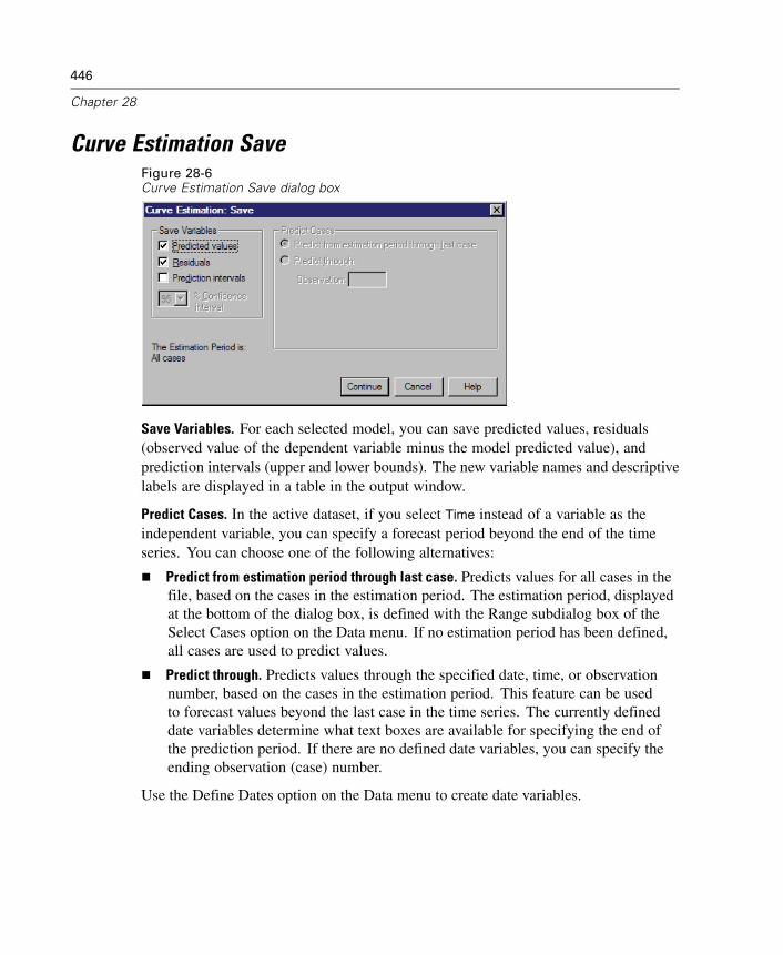
446

Chapter 28

Curve Estimation SaveFigure 28-6Curve Estimation Save dialog box

Save Variables. For each selected model, you can save predicted values, residuals(observed value of the dependent variable minus the model predicted value), andprediction intervals (upper and lower bounds). The new variable names and descriptivelabels are displayed in a table in the output window.

Predict Cases. In the active dataset, if you select Time instead of a variable as theindependent variable, you can specify a forecast period beyond the end of the timeseries. You can choose one of the following alternatives:

Predict from estimation period through last case. Predicts values for all cases in thefile, based on the cases in the estimation period. The estimation period, displayedat the bottom of the dialog box, is defined with the Range subdialog box of theSelect Cases option on the Data menu. If no estimation period has been defined,all cases are used to predict values.

Predict through. Predicts values through the specified date, time, or observationnumber, based on the cases in the estimation period. This feature can be usedto forecast values beyond the last case in the time series. The currently defineddate variables determine what text boxes are available for specifying the end ofthe prediction period. If there are no defined date variables, you can specify theending observation (case) number.

Use the Define Dates option on the Data menu to create date variables.

Chapter

29Discriminant Analysis

Discriminant analysis is useful for building a predictive model of group membershipbased on observed characteristics of each case. The procedure generates a discriminantfunction (or, for more than two groups, a set of discriminant functions) based onlinear combinations of the predictor variables that provide the best discriminationbetween the groups. The functions are generated from a sample of cases for whichgroup membership is known; the functions can then be applied to new cases that havemeasurements for the predictor variables but have unknown group membership.

Note: The grouping variable can have more than two values. The codes for thegrouping variable must be integers, however, and you need to specify their minimumand maximum values. Cases with values outside of these bounds are excluded from theanalysis.

Example. On average, people in temperate zone countries consume more calories perday than people in the tropics, and a greater proportion of the people in the temperatezones are city dwellers. A researcher wants to combine this information into a functionto determine how well an individual can discriminate between the two groups ofcountries. The researcher thinks that population size and economic informationmay also be important. Discriminant analysis allows you to estimate coefficients ofthe linear discriminant function, which looks like the right side of a multiple linearregression equation. That is, using coefficients a, b, c, and d, the function is:

D = a * climate + b * urban + c * population + d * gross domestic product per capita

If these variables are useful for discriminating between the two climate zones, thevalues of D will differ for the temperate and tropic countries. If you use a stepwisevariable selection method, you may find that you do not need to include all fourvariables in the function.

447

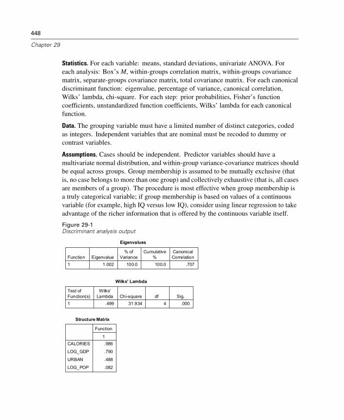
448

Chapter 29

Statistics. For each variable: means, standard deviations, univariate ANOVA. Foreach analysis: Box’s M, within-groups correlation matrix, within-groups covariancematrix, separate-groups covariance matrix, total covariance matrix. For each canonicaldiscriminant function: eigenvalue, percentage of variance, canonical correlation,Wilks’ lambda, chi-square. For each step: prior probabilities, Fisher’s functioncoefficients, unstandardized function coefficients, Wilks’ lambda for each canonicalfunction.

Data. The grouping variable must have a limited number of distinct categories, codedas integers. Independent variables that are nominal must be recoded to dummy orcontrast variables.

Assumptions. Cases should be independent. Predictor variables should have amultivariate normal distribution, and within-group variance-covariance matrices shouldbe equal across groups. Group membership is assumed to be mutually exclusive (thatis, no case belongs to more than one group) and collectively exhaustive (that is, all casesare members of a group). The procedure is most effective when group membership isa truly categorical variable; if group membership is based on values of a continuousvariable (for example, high IQ versus low IQ), consider using linear regression to takeadvantage of the richer information that is offered by the continuous variable itself.

Figure 29-1Discriminant analysis output

1.002 100.0 100.0 .707Function1

Eigenvalue% of

VarianceCumulative

%CanonicalCorrelation

Eigenvalues

.499 31.934 4 .000

Test ofFunction(s)1

Wilks'Lambda Chi-square df Sig.

Wilks' Lambda

.986

.790

.488

.082

CALORIES

LOG_GDP

URBAN

LOG_POP

1

Function

Structure Matrix

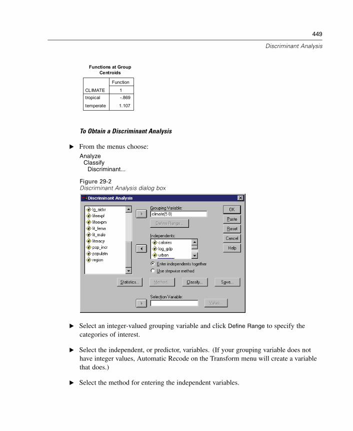
449

Discriminant Analysis

-.869

1.107

CLIMATEtropical

temperate

1

Function

Functions at GroupCentroids

To Obtain a Discriminant Analysis


ClassifyDiscriminant...

Figure 29-2Discriminant Analysis dialog box

E Select an integer-valued grouping variable and click Define Range to specify thecategories of interest.

E Select the independent, or predictor, variables. (If your grouping variable does nothave integer values, Automatic Recode on the Transform menu will create a variablethat does.)

E Select the method for entering the independent variables.

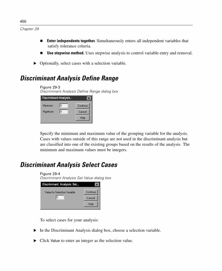
450

Chapter 29

Enter independents together. Simultaneously enters all independent variables thatsatisfy tolerance criteria.

Use stepwise method. Uses stepwise analysis to control variable entry and removal.

E Optionally, select cases with a selection variable.

Discriminant Analysis Define RangeFigure 29-3Discriminant Analysis Define Range dialog box

Specify the minimum and maximum value of the grouping variable for the analysis.Cases with values outside of this range are not used in the discriminant analysis butare classified into one of the existing groups based on the results of the analysis. Theminimum and maximum values must be integers.

Discriminant Analysis Select CasesFigure 29-4Discriminant Analysis Set Value dialog box

To select cases for your analysis:

E In the Discriminant Analysis dialog box, choose a selection variable.

E Click Value to enter an integer as the selection value.

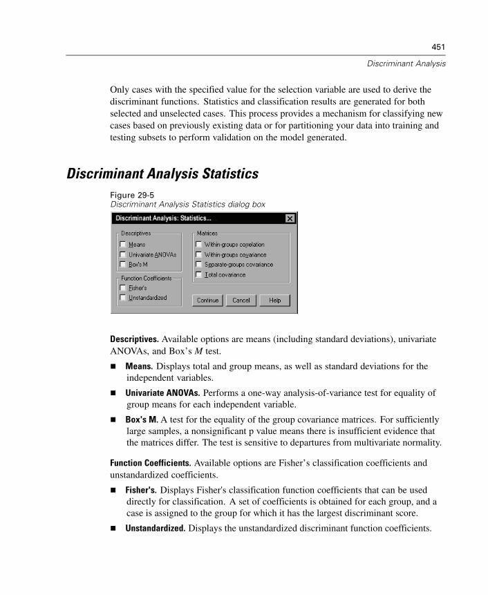
451


Only cases with the specified value for the selection variable are used to derive thediscriminant functions. Statistics and classification results are generated for bothselected and unselected cases. This process provides a mechanism for classifying newcases based on previously existing data or for partitioning your data into training andtesting subsets to perform validation on the model generated.

Discriminant Analysis StatisticsFigure 29-5Discriminant Analysis Statistics dialog box

Descriptives. Available options are means (including standard deviations), univariateANOVAs, and Box’s M test.

Means. Displays total and group means, as well as standard deviations for theindependent variables.

Univariate ANOVAs. Performs a one-way analysis-of-variance test for equality ofgroup means for each independent variable.

Box's M. A test for the equality of the group covariance matrices. For sufficientlylarge samples, a nonsignificant p value means there is insufficient evidence thatthe matrices differ. The test is sensitive to departures from multivariate normality.

Function Coefficients. Available options are Fisher’s classification coefficients andunstandardized coefficients.

Fisher's. Displays Fisher's classification function coefficients that can be useddirectly for classification. A set of coefficients is obtained for each group, and acase is assigned to the group for which it has the largest discriminant score.

Unstandardized. Displays the unstandardized discriminant function coefficients.

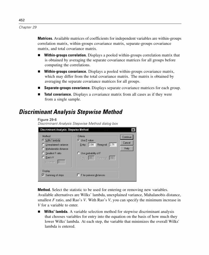
452

Chapter 29

Matrices. Available matrices of coefficients for independent variables are within-groupscorrelation matrix, within-groups covariance matrix, separate-groups covariancematrix, and total covariance matrix.

Within-groups correlation. Displays a pooled within-groups correlation matrix thatis obtained by averaging the separate covariance matrices for all groups beforecomputing the correlations.

Within-groups covariance. Displays a pooled within-groups covariance matrix,which may differ from the total covariance matrix. The matrix is obtained byaveraging the separate covariance matrices for all groups.

Separate-groups covariance. Displays separate covariance matrices for each group.

Total covariance. Displays a covariance matrix from all cases as if they werefrom a single sample.

Discriminant Analysis Stepwise MethodFigure 29-6Discriminant Analysis Stepwise Method dialog box

Method. Select the statistic to be used for entering or removing new variables.Available alternatives are Wilks’ lambda, unexplained variance, Mahalanobis distance,smallest F ratio, and Rao’s V. With Rao’s V, you can specify the minimum increase inV for a variable to enter.

Wilks' lambda. A variable selection method for stepwise discriminant analysisthat chooses variables for entry into the equation on the basis of how much theylower Wilks' lambda. At each step, the variable that minimizes the overall Wilks'lambda is entered.

453


Unexplained variance. At each step, the variable that minimizes the sum of theunexplained variation between groups is entered.

Mahalanobis distance. A measure of how much a case's values on the independentvariables differ from the average of all cases. A large Mahalanobis distanceidentifies a case as having extreme values on one or more of the independentvariables.

Smallest F ratio. A method of variable selection in stepwise analysis based onmaximizing an F ratio computed from the Mahalanobis distance between groups.

Rao's V. A measure of the differences between group means. Also called theLawley-Hotelling trace. At each step, the variable that maximizes the increase inRao's V is entered. After selecting this option, enter the minimum value a variablemust have to enter the analysis.

Criteria. Available alternatives are Use F value and Use probability of F. Enter values forentering and removing variables.

Use F value. A variable is entered into the model if its F value is greater than theEntry value and is removed if the F value is less than the Removal value. Entrymust be greater than Removal, and both values must be positive. To enter morevariables into the model, lower the Entry value. To remove more variables fromthe model, increase the Removal value.

Use probability of F. A variable is entered into the model if the significance level ofits F value is less than the Entry value and is removed if the significance level isgreater than the Removal value. Entry must be less than Removal, and both valuesmust be positive. To enter more variables into the model, increase the Entry value.To remove more variables from the model, lower the Removal value.

Display. Summary of steps displays statistics for all variables after each step; F for

pairwise distances displays a matrix of pairwise F ratios for each pair of groups.

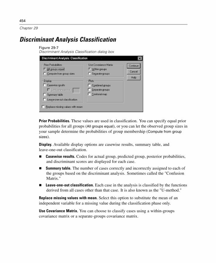
454

Chapter 29

Discriminant Analysis ClassificationFigure 29-7Discriminant Analysis Classification dialog box

Prior Probabilities. These values are used in classification. You can specify equal priorprobabilities for all groups (All groups equal), or you can let the observed group sizes inyour sample determine the probabilities of group membership (Compute from group

sizes).

Display. Available display options are casewise results, summary table, andleave-one-out classification.

Casewise results. Codes for actual group, predicted group, posterior probabilities,and discriminant scores are displayed for each case.

Summary table. The number of cases correctly and incorrectly assigned to each ofthe groups based on the discriminant analysis. Sometimes called the "ConfusionMatrix."

Leave-one-out classification. Each case in the analysis is classified by the functionsderived from all cases other than that case. It is also known as the "U-method."

Replace missing values with mean. Select this option to substitute the mean of anindependent variable for a missing value during the classification phase only.

Use Covariance Matrix. You can choose to classify cases using a within-groupscovariance matrix or a separate-groups covariance matrix.

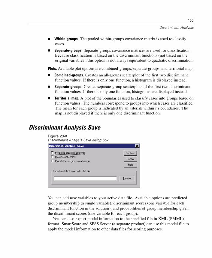
455


Within-groups. The pooled within-groups covariance matrix is used to classifycases.

Separate-groups. Separate-groups covariance matrices are used for classification.Because classification is based on the discriminant functions (not based on theoriginal variables), this option is not always equivalent to quadratic discrimination.

Plots. Available plot options are combined-groups, separate-groups, and territorial map.

Combined-groups. Creates an all-groups scatterplot of the first two discriminantfunction values. If there is only one function, a histogram is displayed instead.

Separate-groups. Creates separate-group scatterplots of the first two discriminantfunction values. If there is only one function, histograms are displayed instead.

Territorial map. A plot of the boundaries used to classify cases into groups based onfunction values. The numbers correspond to groups into which cases are classified.The mean for each group is indicated by an asterisk within its boundaries. Themap is not displayed if there is only one discriminant function.

Discriminant Analysis SaveFigure 29-8Discriminant Analysis Save dialog box

You can add new variables to your active data file. Available options are predictedgroup membership (a single variable), discriminant scores (one variable for eachdiscriminant function in the solution), and probabilities of group membership giventhe discriminant scores (one variable for each group).

You can also export model information to the specified file in XML (PMML)format. SmartScore and SPSS Server (a separate product) can use this model file toapply the model information to other data files for scoring purposes.

456

Chapter 29

DISCRIMINANT Command Additional Features


Perform multiple discriminant analyses (with one command) and control the orderin which variables are entered (with the ANALYSIS subcommand).

Specify prior probabilities for classification (with the PRIORS subcommand).

Display rotated pattern and structure matrices (with the ROTATE subcommand).

Limit the number of extracted discriminant functions (with the FUNCTIONSsubcommand).

Restrict classification to the cases that are selected (or unselected) for the analysis(with the SELECT subcommand).

Read and analyze a correlation matrix (with the MATRIX subcommand).

Write a correlation matrix for later analysis (with the MATRIX subcommand).


Chapter

30Factor Analysis

Factor analysis attempts to identify underlying variables, or factors, that explain thepattern of correlations within a set of observed variables. Factor analysis is oftenused in data reduction to identify a small number of factors that explain most ofthe variance that is observed in a much larger number of manifest variables. Factoranalysis can also be used to generate hypotheses regarding causal mechanisms or toscreen variables for subsequent analysis (for example, to identify collinearity prior toperforming a linear regression analysis).

The factor analysis procedure offers a high degree of flexibility:

Seven methods of factor extraction are available.

Five methods of rotation are available, including direct oblimin and promax fornonorthogonal rotations.

Three methods of computing factor scores are available, and scores can be saved asvariables for further analysis.

Example. What underlying attitudes lead people to respond to the questions on apolitical survey as they do? Examining the correlations among the survey itemsreveals that there is significant overlap among various subgroups of items—questionsabout taxes tend to correlate with each other, questions about military issues correlatewith each other, and so on. With factor analysis, you can investigate the number ofunderlying factors and, in many cases, you can identify what the factors representconceptually. Additionally, you can compute factor scores for each respondent, whichcan then be used in subsequent analyses. For example, you might build a logisticregression model to predict voting behavior based on factor scores.

Statistics. For each variable: number of valid cases, mean, and standard deviation.For each factor analysis: correlation matrix of variables, including significancelevels, determinant, and inverse; reproduced correlation matrix, including anti-image;initial solution (communalities, eigenvalues, and percentage of variance explained);Kaiser-Meyer-Olkin measure of sampling adequacy and Bartlett’s test of sphericity;

457

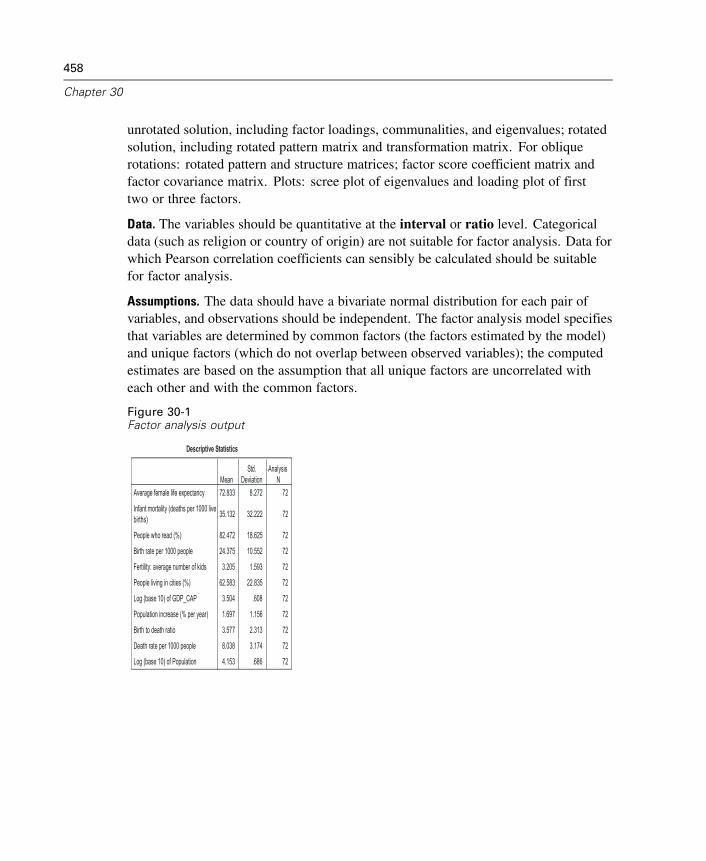
458

Chapter 30

unrotated solution, including factor loadings, communalities, and eigenvalues; rotatedsolution, including rotated pattern matrix and transformation matrix. For obliquerotations: rotated pattern and structure matrices; factor score coefficient matrix andfactor covariance matrix. Plots: scree plot of eigenvalues and loading plot of firsttwo or three factors.

Data. The variables should be quantitative at the interval or ratio level. Categoricaldata (such as religion or country of origin) are not suitable for factor analysis. Data forwhich Pearson correlation coefficients can sensibly be calculated should be suitablefor factor analysis.

Assumptions. The data should have a bivariate normal distribution for each pair ofvariables, and observations should be independent. The factor analysis model specifiesthat variables are determined by common factors (the factors estimated by the model)and unique factors (which do not overlap between observed variables); the computedestimates are based on the assumption that all unique factors are uncorrelated witheach other and with the common factors.

Figure 30-1Factor analysis output

72.833 8.272 72

35.132 32.222 72

82.472 18.625 72

24.375 10.552 72

3.205 1.593 72

62.583 22.835 72

3.504 .608 72

1.697 1.156 72

3.577 2.313 72

8.038 3.174 72

4.153 .686 72

Average female life expectancy

Infant mortality (deaths per 1000 livebirths)

People who read (%)

Birth rate per 1000 people

Fertility: average number of kids

People living in cities (%)

Log (base 10) of GDP_CAP

Population increase (% per year)

Birth to death ratio

Death rate per 1000 people

Log (base 10) of Population

MeanStd.

DeviationAnalysis

N

Descriptive Statistics

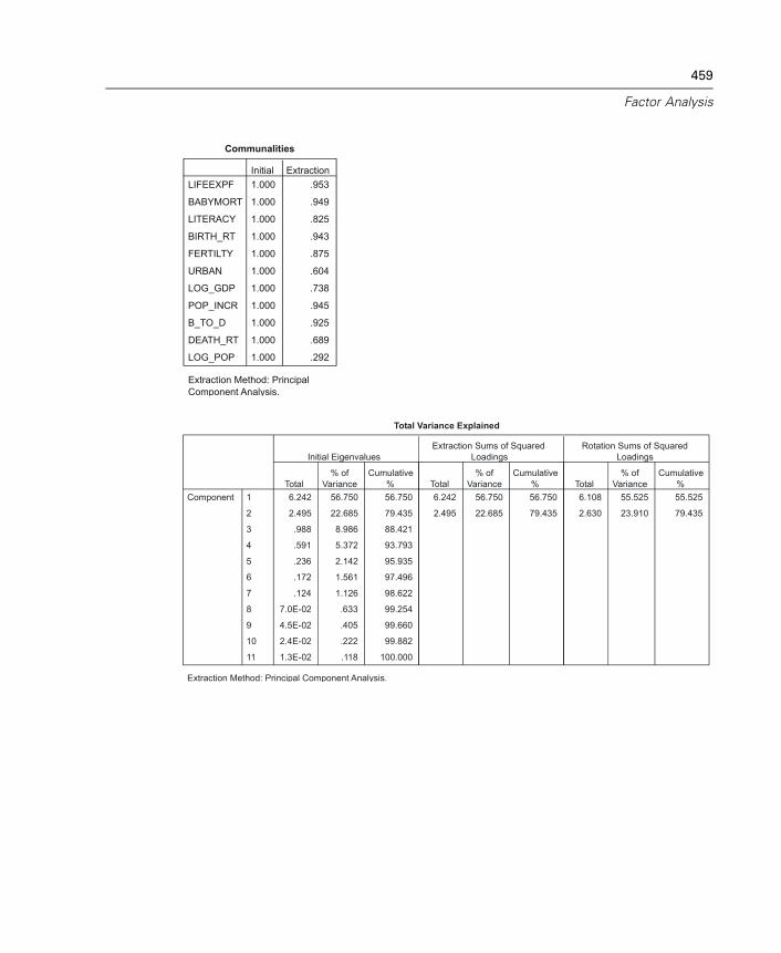
459

Factor Analysis

1.000 .953

1.000 .949

1.000 .825

1.000 .943

1.000 .875

1.000 .604

1.000 .738

1.000 .945

1.000 .925

1.000 .689

1.000 .292

LIFEEXPF

BABYMORT

LITERACY

BIRTH_RT

FERTILTY

URBAN

LOG_GDP

POP_INCR

B_TO_D

DEATH_RT

LOG_POP

Initial Extraction

Communalities

Extraction Method: PrincipalComponent Analysis.

6.242 56.750 56.750 6.242 56.750 56.750 6.108 55.525 55.525

2.495 22.685 79.435 2.495 22.685 79.435 2.630 23.910 79.435

.988 8.986 88.421

.591 5.372 93.793

.236 2.142 95.935

.172 1.561 97.496

.124 1.126 98.622

7.0E-02 .633 99.254

4.5E-02 .405 99.660

2.4E-02 .222 99.882

1.3E-02 .118 100.000

1

2

3

4

5

6

7

8

9

10

11

ComponentTotal

% ofVariance

Cumulative% Total

% ofVariance

Cumulative% Total

% ofVariance

Cumulative%

Initial EigenvaluesExtraction Sums of Squared

LoadingsRotation Sums of Squared

Loadings

Total Variance Explained

Extraction Method: Principal Component Analysis.

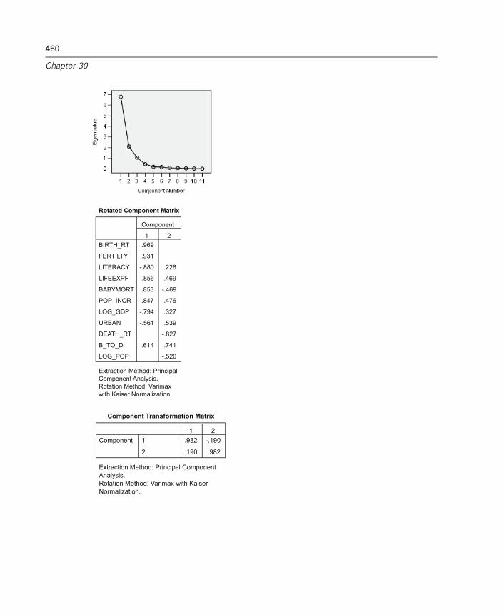
460

Chapter 30

.969

.931

-.880 .226

-.856 .469

.853 -.469

.847 .476

-.794 .327

-.561 .539

-.827

.614 .741

-.520

BIRTH_RT

FERTILTY

LITERACY

LIFEEXPF

BABYMORT

POP_INCR

LOG_GDP

URBAN

DEATH_RT

B_TO_D

LOG_POP

1 2

Component

Rotated Component Matrix

Extraction Method: PrincipalComponent Analysis. Rotation Method: Varimaxwith Kaiser Normalization.

.982 -.190

.190 .982

1

2

Component1 2

Component Transformation Matrix

Extraction Method: Principal ComponentAnalysis. Rotation Method: Varimax with KaiserNormalization.

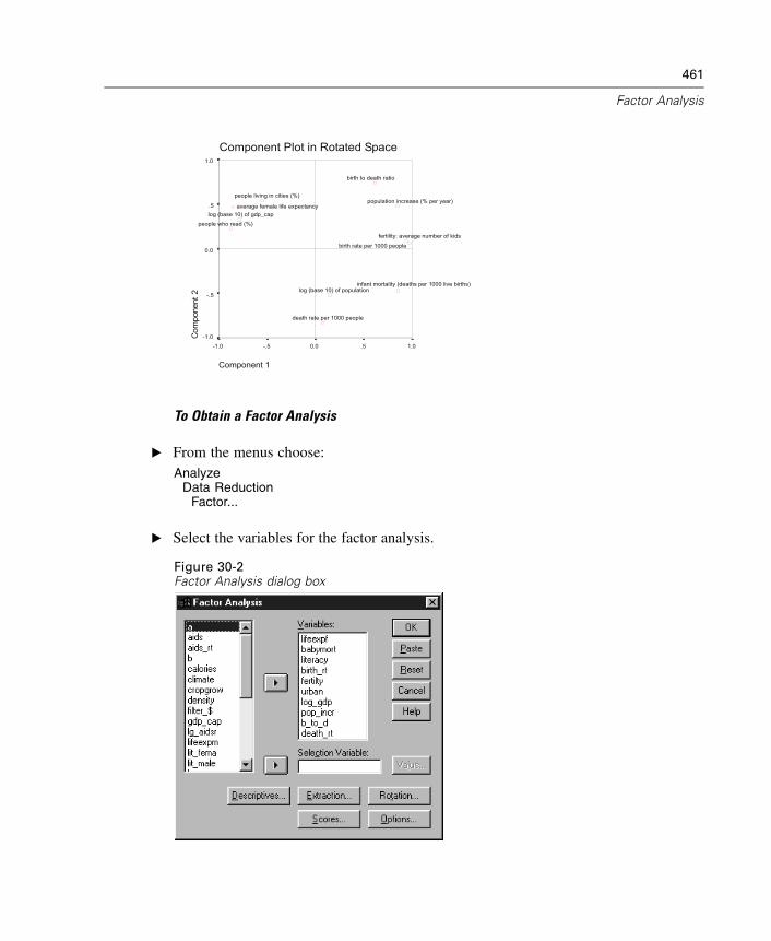
461

Factor Analysis

Component Plot in Rotated Space

Component 1

1.0.50.0-.5-1.0

Com

pone

nt2

1.0

.5

0.0

-.5

-1.0

log (base 10) of population

death rate per 1000 people

birth to death ratio

population increase (% per year)

log (base 10) of gdp_cap

people living in cities (%)

fertility: average number of kids

birth rate per 1000 people

people who read (%)

infant mortality (deaths per 1000 live births)

average female life expectancy

To Obtain a Factor Analysis


Data ReductionFactor...

E Select the variables for the factor analysis.

Figure 30-2Factor Analysis dialog box

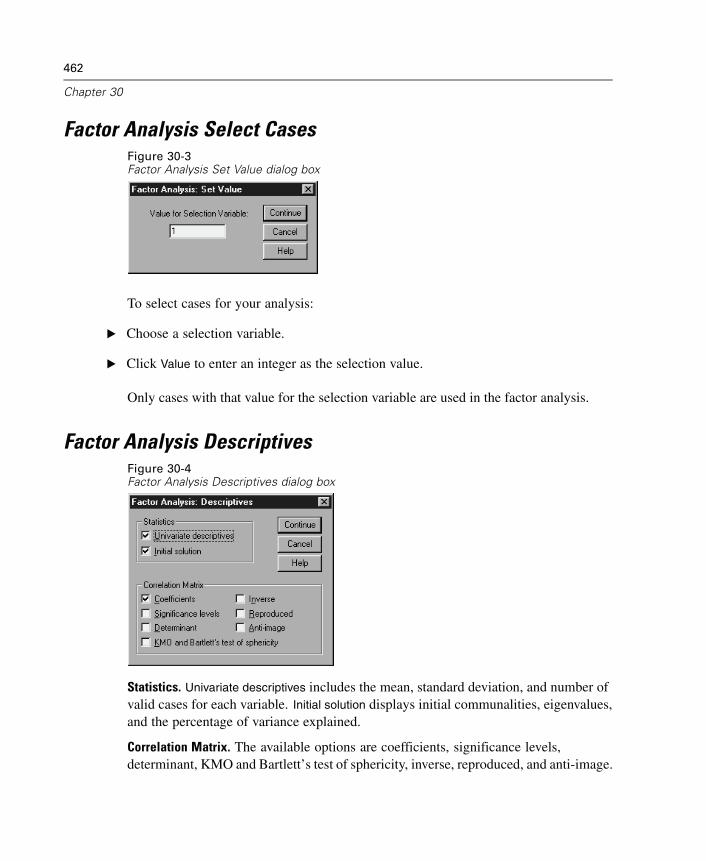
462

Chapter 30

Factor Analysis Select CasesFigure 30-3Factor Analysis Set Value dialog box

To select cases for your analysis:

E Choose a selection variable.

E Click Value to enter an integer as the selection value.

Only cases with that value for the selection variable are used in the factor analysis.

Factor Analysis DescriptivesFigure 30-4Factor Analysis Descriptives dialog box

Statistics. Univariate descriptives includes the mean, standard deviation, and number ofvalid cases for each variable. Initial solution displays initial communalities, eigenvalues,and the percentage of variance explained.

Correlation Matrix. The available options are coefficients, significance levels,determinant, KMO and Bartlett’s test of sphericity, inverse, reproduced, and anti-image.

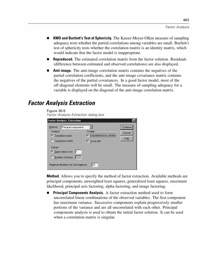
463

Factor Analysis

KMO and Bartlett's Test of Sphericity. The Kaiser-Meyer-Olkin measure of samplingadequacy tests whether the partial correlations among variables are small. Bartlett'stest of sphericity tests whether the correlation matrix is an identity matrix, whichwould indicate that the factor model is inappropriate.

Reproduced. The estimated correlation matrix from the factor solution. Residuals(difference between estimated and observed correlations) are also displayed.

Anti-image. The anti-image correlation matrix contains the negatives of thepartial correlation coefficients, and the anti-image covariance matrix containsthe negatives of the partial covariances. In a good factor model, most of theoff-diagonal elements will be small. The measure of sampling adequacy for avariable is displayed on the diagonal of the anti-image correlation matrix.

Factor Analysis ExtractionFigure 30-5Factor Analysis Extraction dialog box

Method. Allows you to specify the method of factor extraction. Available methods areprincipal components, unweighted least squares, generalized least squares, maximumlikelihood, principal axis factoring, alpha factoring, and image factoring.

Principal Components Analysis. A factor extraction method used to formuncorrelated linear combinations of the observed variables. The first componenthas maximum variance. Successive components explain progressively smallerportions of the variance and are all uncorrelated with each other. Principalcomponents analysis is used to obtain the initial factor solution. It can be usedwhen a correlation matrix is singular.

464

Chapter 30

Unweighted Least-Squares Method. A factor extraction method that minimizes thesum of the squared differences between the observed and reproduced correlationmatrices (ignoring the diagonals).

Generalized Least-Squares Method. A factor extraction method that minimizes thesum of the squared differences between the observed and reproduced correlationmatrices. Correlations are weighted by the inverse of their uniqueness, sothat variables with high uniqueness are given less weight than those with lowuniqueness.

Maximum-Likelihood Method. A factor extraction method that produces parameterestimates that are most likely to have produced the observed correlation matrixif the sample is from a multivariate normal distribution. The correlations areweighted by the inverse of the uniqueness of the variables, and an iterativealgorithm is employed.

Principal Axis Factoring. A method of extracting factors from the originalcorrelation matrix, with squared multiple correlation coefficients placed in thediagonal as initial estimates of the communalities. These factor loadings are usedto estimate new communalities that replace the old communality estimates in thediagonal. Iterations continue until the changes in the communalities from oneiteration to the next satisfy the convergence criterion for extraction.

Alpha. A factor extraction method that considers the variables in the analysis tobe a sample from the universe of potential variables. This method maximizes thealpha reliability of the factors.

Image Factoring. A factor extraction method developed by Guttman and basedon image theory. The common part of the variable, called the partial image,is defined as its linear regression on remaining variables, rather than a functionof hypothetical factors.

Analyze. Allows you to specify either a correlation matrix or a covariance matrix.

Correlation matrix. Useful if variables in your analysis are measured on differentscales.

Covariance matrix. Useful when you want to apply your factor analysis to multiplegroups with different variances for each variable.

Extract. You can either retain all factors whose eigenvalues exceed a specified value, oryou can retain a specific number of factors.

Display. Allows you to request the unrotated factor solution and a scree plot of theeigenvalues.

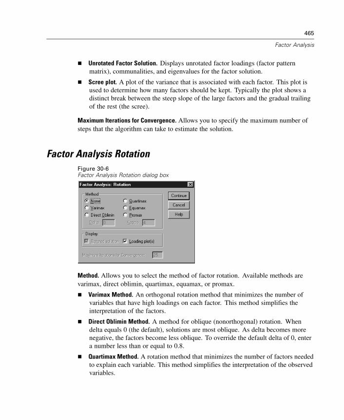
465

Factor Analysis

Unrotated Factor Solution. Displays unrotated factor loadings (factor patternmatrix), communalities, and eigenvalues for the factor solution.

Scree plot. A plot of the variance that is associated with each factor. This plot isused to determine how many factors should be kept. Typically the plot shows adistinct break between the steep slope of the large factors and the gradual trailingof the rest (the scree).

Maximum Iterations for Convergence. Allows you to specify the maximum number ofsteps that the algorithm can take to estimate the solution.

Factor Analysis RotationFigure 30-6Factor Analysis Rotation dialog box

Method. Allows you to select the method of factor rotation. Available methods arevarimax, direct oblimin, quartimax, equamax, or promax.

Varimax Method. An orthogonal rotation method that minimizes the number ofvariables that have high loadings on each factor. This method simplifies theinterpretation of the factors.

Direct Oblimin Method. A method for oblique (nonorthogonal) rotation. Whendelta equals 0 (the default), solutions are most oblique. As delta becomes morenegative, the factors become less oblique. To override the default delta of 0, entera number less than or equal to 0.8.

Quartimax Method. A rotation method that minimizes the number of factors neededto explain each variable. This method simplifies the interpretation of the observedvariables.

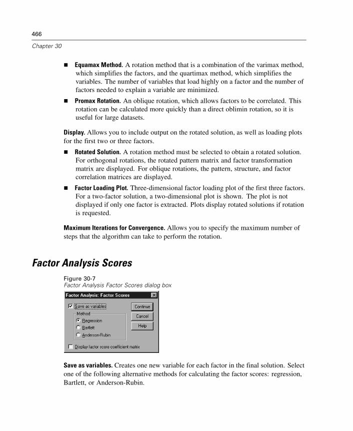
466

Chapter 30

Equamax Method. A rotation method that is a combination of the varimax method,which simplifies the factors, and the quartimax method, which simplifies thevariables. The number of variables that load highly on a factor and the number offactors needed to explain a variable are minimized.

Promax Rotation. An oblique rotation, which allows factors to be correlated. Thisrotation can be calculated more quickly than a direct oblimin rotation, so it isuseful for large datasets.

Display. Allows you to include output on the rotated solution, as well as loading plotsfor the first two or three factors.

Rotated Solution. A rotation method must be selected to obtain a rotated solution.For orthogonal rotations, the rotated pattern matrix and factor transformationmatrix are displayed. For oblique rotations, the pattern, structure, and factorcorrelation matrices are displayed.

Factor Loading Plot. Three-dimensional factor loading plot of the first three factors.For a two-factor solution, a two-dimensional plot is shown. The plot is notdisplayed if only one factor is extracted. Plots display rotated solutions if rotationis requested.

Maximum Iterations for Convergence. Allows you to specify the maximum number ofsteps that the algorithm can take to perform the rotation.

Factor Analysis ScoresFigure 30-7Factor Analysis Factor Scores dialog box

Save as variables. Creates one new variable for each factor in the final solution. Selectone of the following alternative methods for calculating the factor scores: regression,Bartlett, or Anderson-Rubin.

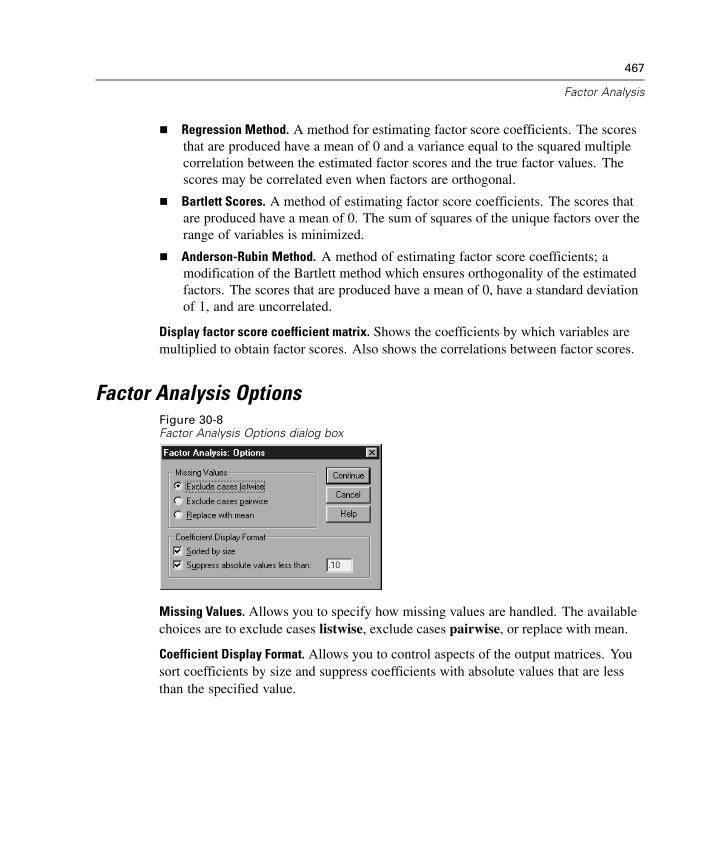
467

Factor Analysis

Regression Method. A method for estimating factor score coefficients. The scoresthat are produced have a mean of 0 and a variance equal to the squared multiplecorrelation between the estimated factor scores and the true factor values. Thescores may be correlated even when factors are orthogonal.

Bartlett Scores. A method of estimating factor score coefficients. The scores thatare produced have a mean of 0. The sum of squares of the unique factors over therange of variables is minimized.

Anderson-Rubin Method. A method of estimating factor score coefficients; amodification of the Bartlett method which ensures orthogonality of the estimatedfactors. The scores that are produced have a mean of 0, have a standard deviationof 1, and are uncorrelated.

Display factor score coefficient matrix. Shows the coefficients by which variables aremultiplied to obtain factor scores. Also shows the correlations between factor scores.

Factor Analysis OptionsFigure 30-8Factor Analysis Options dialog box

Missing Values. Allows you to specify how missing values are handled. The availablechoices are to exclude cases listwise, exclude cases pairwise, or replace with mean.

Coefficient Display Format. Allows you to control aspects of the output matrices. Yousort coefficients by size and suppress coefficients with absolute values that are lessthan the specified value.

468

Chapter 30

FACTOR Command Additional Features


Specify convergence criteria for iteration during extraction and rotation.

Specify individual rotated-factor plots.

Specify how many factor scores to save.

Specify diagonal values for the principal axis factoring method.

Write correlation matrices or factor-loading matrices to disk for later analysis.

Read and analyze correlation matrices or factor-loading matrices.


Chapter

31Choosing a Procedure forClustering

Cluster analyses can be performed using the TwoStep, Hierarchical, or K-MeansCluster Analysis procedure. Each procedure employs a different algorithm for creatingclusters, and each has options not available in the others.

TwoStep Cluster Analysis. For many applications, the TwoStep Cluster Analysisprocedure will be the method of choice. It provides the following unique features:

Automatic selection of the best number of clusters, in addition to measures forchoosing between cluster models.

Ability to create cluster models simultaneously based on categorical andcontinuous variables.

Ability to save the cluster model to an external XML file and then read that file andupdate the cluster model using newer data.

Additionally, the TwoStep Cluster Analysis procedure can analyze large data files.

Hierarchical Cluster Analysis. The Hierarchical Cluster Analysis procedure is limited tosmaller data files (hundreds of objects to be clustered) but has the following uniquefeatures:

Ability to cluster cases or variables.

Ability to compute a range of possible solutions and save cluster memberships foreach of those solutions.

Several methods for cluster formation, variable transformation, and measuring thedissimilarity between clusters.

As long as all the variables are of the same type, the Hierarchical Cluster Analysisprocedure can analyze interval (continuous), count, or binary variables.

469

470

Chapter 31

K-Means Cluster Analysis. The K-Means Cluster Analysis procedure is limited tocontinuous data and requires you to specify the number of clusters in advance, but ithas the following unique features:

Ability to save distances from cluster centers for each object.

Ability to read initial cluster centers from and save final cluster centers to anexternal SPSS file.

Additionally, the K-Means Cluster Analysis procedure can analyze large data files.

Chapter

32TwoStep Cluster Analysis

The TwoStep Cluster Analysis procedure is an exploratory tool designed to revealnatural groupings (or clusters) within a dataset that would otherwise not be apparent.The algorithm employed by this procedure has several desirable features thatdifferentiate it from traditional clustering techniques:

Handling of categorical and continuous variables. By assuming variables to beindependent, a joint multinomial-normal distribution can be placed on categoricaland continuous variables.

Automatic selection of number of clusters. By comparing the values of amodel-choice criterion across different clustering solutions, the procedure canautomatically determine the optimal number of clusters.

Scalability. By constructing a cluster features (CF) tree that summarizes therecords, the TwoStep algorithm allows you to analyze large data files.

Example. Retail and consumer product companies regularly apply clustering techniquesto data that describe their customers’ buying habits, gender, age, income level, etc.These companies tailor their marketing and product development strategies to eachconsumer group to increase sales and build brand loyalty.

Statistics. The procedure produces information criteria (AIC or BIC) by number ofclusters in the solution, cluster frequencies for the final clustering, and descriptivestatistics by cluster for the final clustering.

Plots. The procedure produces bar charts of cluster frequencies, pie charts of clusterfrequencies, and variable importance charts.

471

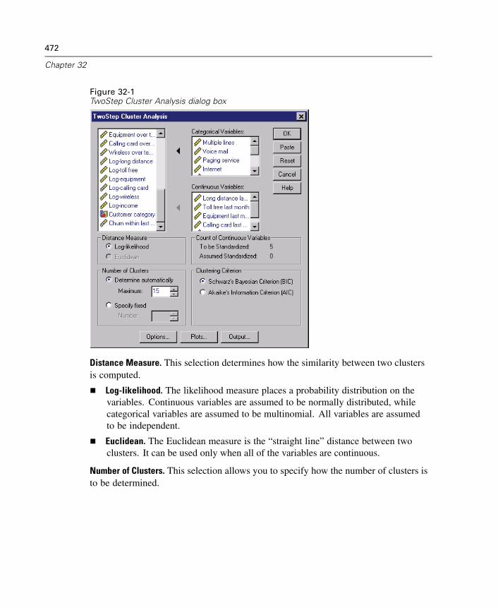
472

Chapter 32

Figure 32-1TwoStep Cluster Analysis dialog box

Distance Measure. This selection determines how the similarity between two clustersis computed.

Log-likelihood. The likelihood measure places a probability distribution on thevariables. Continuous variables are assumed to be normally distributed, whilecategorical variables are assumed to be multinomial. All variables are assumedto be independent.

Euclidean. The Euclidean measure is the “straight line” distance between twoclusters. It can be used only when all of the variables are continuous.

Number of Clusters. This selection allows you to specify how the number of clusters isto be determined.

473

TwoStep Cluster Analysis

Determine automatically. The procedure will automatically determine the “best”number of clusters, using the criterion specified in the Clustering Criterion group.Optionally, enter a positive integer specifying the maximum number of clustersthat the procedure should consider.

Specify fixed. Allows you to fix the number of clusters in the solution. Entera positive integer.

Count of Continuous Variables. This group provides a summary of the continuousvariable standardization specifications made in the Options dialog box. For moreinformation, see “TwoStep Cluster Analysis Options” on p. 475.

Clustering Criterion. This selection determines how the automatic clustering algorithmdetermines the number of clusters. Either the Bayesian Information Criterion (BIC) orthe Akaike Information Criterion (AIC) can be specified.

Data. This procedure works with both continuous and categorical variables. Casesrepresent objects to be clustered, and the variables represent attributes upon whichthe clustering is based.

Case Order. Note that the cluster features tree and the final solution may depend onthe order of cases. To minimize order effects, randomly order the cases. You maywant to obtain several different solutions with cases sorted in different random ordersto verify the stability of a given solution. In situations where this is difficult due toextremely large file sizes, multiple runs with a sample of cases sorted in differentrandom orders might be substituted.

Assumptions. The likelihood distance measure assumes that variables in the clustermodel are independent. Further, each continuous variable is assumed to have a normal(Gaussian) distribution, and each categorical variable is assumed to have a multinomialdistribution. Empirical internal testing indicates that the procedure is fairly robust toviolations of both the assumption of independence and the distributional assumptions,but you should try to be aware of how well these assumptions are met.

Use the Bivariate Correlations procedure to test the independence of two continuousvariables. Use the Crosstabs procedure to test the independence of two categoricalvariables. Use the Means procedure to test the independence between a continuousvariable and categorical variable. Use the Explore procedure to test the normality of acontinuous variable. Use the Chi-Square Test procedure to test whether a categoricalvariable has a specified multinomial distribution.

474

Chapter 32

To Obtain a TwoStep Cluster Analysis


ClassifyTwoStep Cluster...

E Select one or more categorical or continuous variables.


Adjust the criteria by which clusters are constructed.

Select settings for noise handling, memory allocation, variable standardization,and cluster model input.

Request optional tables and plots.

Save model results to the working file or to an external XML file.

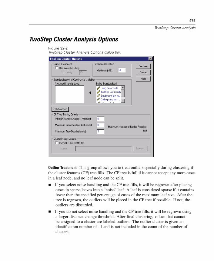
475


TwoStep Cluster Analysis OptionsFigure 32-2TwoStep Cluster Analysis Options dialog box

Outlier Treatment. This group allows you to treat outliers specially during clustering ifthe cluster features (CF) tree fills. The CF tree is full if it cannot accept any more casesin a leaf node, and no leaf node can be split.

If you select noise handling and the CF tree fills, it will be regrown after placingcases in sparse leaves into a “noise” leaf. A leaf is considered sparse if it containsfewer than the specified percentage of cases of the maximum leaf size. After thetree is regrown, the outliers will be placed in the CF tree if possible. If not, theoutliers are discarded.

If you do not select noise handling and the CF tree fills, it will be regrown usinga larger distance change threshold. After final clustering, values that cannotbe assigned to a cluster are labeled outliers. The outlier cluster is given anidentification number of –1 and is not included in the count of the number ofclusters.

476

Chapter 32

Memory Allocation. This group allows you to specify the maximum amount of memoryin megabytes (MB) that the cluster algorithm should use. If the procedure exceeds thismaximum, it will use the disk to store information that will not fit in memory. Specifya number greater than or equal to 4.

Consult your system administrator for the largest value that you can specify onyour system.

The algorithm may fail to find the correct or desired number of clusters if thisvalue is too low.

Variable standardization. The clustering algorithm works with standardized continuousvariables. Any continuous variables that are not standardized should be left as variablesin the To be Standardized list. To save some time and computational effort, you canselect any continuous variables that you have already standardized as variables inthe Assumed Standardized list.

Advanced Options

CF Tree Tuning Criteria. The following clustering algorithm settings apply specifically tothe cluster features (CF) tree and should be changed with care:

Initial Distance Change Threshold. This is the initial threshold used to grow the CFtree. If inserting a given case into a leaf of the CF tree would yield tightness lessthan the threshold, the leaf is not split. If the tightness exceeds the threshold,the leaf is split.

Maximum Branches (per leaf node). The maximum number of child nodes thata leaf node can have.

Maximum Tree Depth. The maximum number of levels that the CF tree can have.

Maximum Number of Nodes Possible. This indicates the maximum number of CFtree nodes that could potentially be generated by the procedure, based on thefunction (bd+1 – 1) / (b – 1), where b is the maximum branches and d is themaximum tree depth. Be aware that an overly large CF tree can be a drain onsystem resources and can adversely affect the performance of the procedure. At aminimum, each node requires 16 bytes.

Cluster Model Update. This group allows you to import and update a cluster modelgenerated in a prior analysis. The input file contains the CF tree in XML format. Themodel will then be updated with the data in the active file. You must select the variablenames in the main dialog box in the same order in which they were specified in the

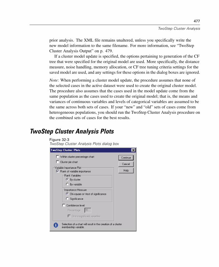
477


prior analysis. The XML file remains unaltered, unless you specifically write thenew model information to the same filename. For more information, see “TwoStepCluster Analysis Output” on p. 479.

If a cluster model update is specified, the options pertaining to generation of the CFtree that were specified for the original model are used. More specifically, the distancemeasure, noise handling, memory allocation, or CF tree tuning criteria settings for thesaved model are used, and any settings for these options in the dialog boxes are ignored.

Note: When performing a cluster model update, the procedure assumes that none ofthe selected cases in the active dataset were used to create the original cluster model.The procedure also assumes that the cases used in the model update come from thesame population as the cases used to create the original model; that is, the means andvariances of continuous variables and levels of categorical variables are assumed to bethe same across both sets of cases. If your “new” and “old” sets of cases come fromheterogeneous populations, you should run the TwoStep Cluster Analysis procedure onthe combined sets of cases for the best results.

TwoStep Cluster Analysis PlotsFigure 32-3TwoStep Cluster Analysis Plots dialog box

478

Chapter 32

Within cluster percentage chart. Displays charts showing the within-cluster variation ofeach variable. For each categorical variable, a clustered bar chart is produced, showingthe category frequency by cluster ID. For each continuous variable, an error bar chartis produced, showing error bars by cluster ID.

Cluster pie chart. Displays a pie chart showing the percentage and counts ofobservations within each cluster.

Variable Importance Plot. Displays several different charts showing the importance ofeach variable within each cluster. The output is sorted by the importance rank ofeach variable.

Rank Variables. This option determines whether plots will be created for eachcluster (By variable) or for each variable (By cluster).

Importance Measure. This option allows you to select which measure of variableimportance to plot. Chi-square or t-test of significance reports a Pearson chi-squarestatistic as the importance of a categorical variable and a t statistic as theimportance of a continuous variable. Significance reports one minus the p value forthe test of equality of means for a continuous variable and the expected frequencywith the overall dataset for a categorical variable.

Confidence level. This option allows you to set the confidence level for the test ofequality of a variable’s distribution within a cluster versus the variable’s overalldistribution. Specify a number less than 100 and greater than or equal to 50. Thevalue of the confidence level is shown as a vertical line in the variable importanceplots, if the plots are created by variable or if the significance measure is plotted.

Omit insignificant variables. Variables that are not significant at the specifiedconfidence level are not displayed in the variable importance plots.

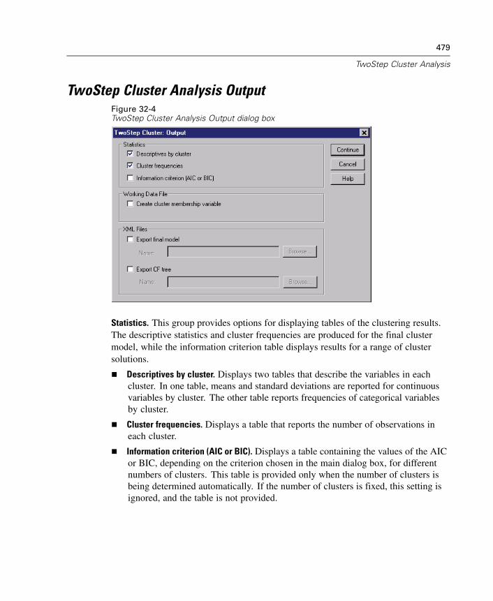
479


TwoStep Cluster Analysis OutputFigure 32-4TwoStep Cluster Analysis Output dialog box

Statistics. This group provides options for displaying tables of the clustering results.The descriptive statistics and cluster frequencies are produced for the final clustermodel, while the information criterion table displays results for a range of clustersolutions.

Descriptives by cluster. Displays two tables that describe the variables in eachcluster. In one table, means and standard deviations are reported for continuousvariables by cluster. The other table reports frequencies of categorical variablesby cluster.

Cluster frequencies. Displays a table that reports the number of observations ineach cluster.

Information criterion (AIC or BIC). Displays a table containing the values of the AICor BIC, depending on the criterion chosen in the main dialog box, for differentnumbers of clusters. This table is provided only when the number of clusters isbeing determined automatically. If the number of clusters is fixed, this setting isignored, and the table is not provided.

480

Chapter 32

Active dataset. This group allows you to save variables to the active dataset.

Create cluster membership variable. This variable contains a cluster identificationnumber for each case. The name of this variable is tsc_n, where n is a positiveinteger indicating the ordinal of the active dataset save operation completed by thisprocedure in a given session.

XML Files. The final cluster model and CF tree are two types of output files that can beexported in XML format.

Export final model. The final cluster model is exported to the specified file in XML(PMML) format. SmartScore and SPSS Server (a separate product) can use thismodel file to apply the model information to other data files for scoring purposes.

Export CF tree. This option allows you to save the current state of the cluster treeand update it later using newer data.

Chapter

33Hierarchical Cluster Analysis

This procedure attempts to identify relatively homogeneous groups of cases (orvariables) based on selected characteristics, using an algorithm that starts with eachcase (or variable) in a separate cluster and combines clusters until only one is left.You can analyze raw variables or you can choose from a variety of standardizingtransformations. Distance or similarity measures are generated by the Proximitiesprocedure. Statistics are displayed at each stage to help you select the best solution.

Example. Are there identifiable groups of television shows that attract similaraudiences within each group? With hierarchical cluster analysis, you could clustertelevision shows (cases) into homogeneous groups based on viewer characteristics.This can be used to identify segments for marketing. Or you can cluster cities (cases)into homogeneous groups so that comparable cities can be selected to test variousmarketing strategies.

Statistics. Agglomeration schedule, distance (or similarity) matrix, and clustermembership for a single solution or a range of solutions. Plots: dendrograms andicicle plots.

Data. The variables can be quantitative, binary, or count data. Scaling of variables isan important issue—differences in scaling may affect your cluster solution(s). If yourvariables have large differences in scaling (for example, one variable is measured indollars and the other is measured in years), you should consider standardizing them(this can be done automatically by the Hierarchical Cluster Analysis procedure).

Case Order. If tied distances or similarities exist in the input data or occur amongupdated clusters during joining, the resulting cluster solution may depend on the orderof cases in the file. You may want to obtain several different solutions with cases sortedin different random orders to verify the stability of a given solution.

Assumptions. The distance or similarity measures used should be appropriate for thedata analyzed (see the Proximities procedure for more information on choices ofdistance and similarity measures). Also, you should include all relevant variables in

481

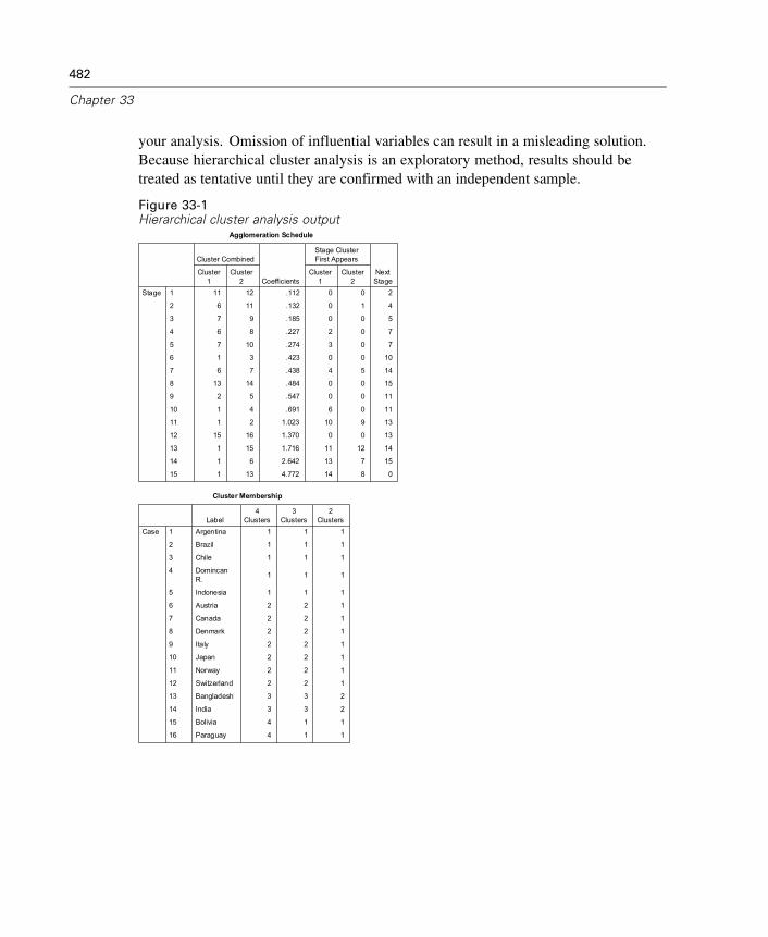
482

Chapter 33

your analysis. Omission of influential variables can result in a misleading solution.Because hierarchical cluster analysis is an exploratory method, results should betreated as tentative until they are confirmed with an independent sample.

Figure 33-1Hierarchical cluster analysis output

11 12 .112 0 0 2

6 11 .132 0 1 4

7 9 .185 0 0 5

6 8 .227 2 0 7

7 10 .274 3 0 7

1 3 .423 0 0 10

6 7 .438 4 5 14

13 14 .484 0 0 15

2 5 .547 0 0 11

1 4 .691 6 0 11

1 2 1.023 10 9 13

15 16 1.370 0 0 13

1 15 1.716 11 12 14

1 6 2.642 13 7 15

1 13 4.772 14 8 0

1

2

3

4

5

6

7

8

9

10

11

12

13

14

15

Stage

Cluster1

Cluster2

Cluster Combined

CoefficientsCluster

1Cluster

2

Stage ClusterFirst Appears

NextStage

Agglomeration Schedule

Argentina 1 1 1

Brazil 1 1 1

Chile 1 1 1

DomincanR. 1 1 1

Indonesia 1 1 1

Austria 2 2 1

Canada 2 2 1

Denmark 2 2 1

Italy 2 2 1

Japan 2 2 1

Norway 2 2 1

Switzerland 2 2 1

Bangladesh 3 3 2

India 3 3 2

Bolivia 4 1 1

Paraguay 4 1 1

1

2

3

4

5

6

7

8

9

10

11

12

13

14

15

16

CaseLabel

4Clusters

3Clusters

2Clusters

Cluster Membership

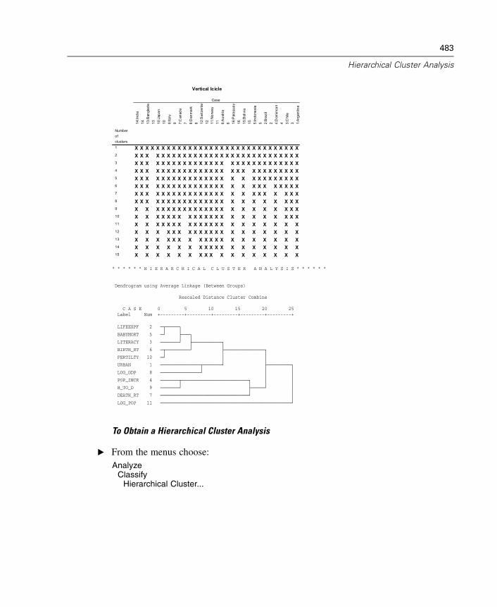
483

Hierarchical Cluster Analysis

X X X X X X X X X X X X X X X X X X X X X X X X X X X X X X XX X X X X X X X X X X X X X X X X X X X X X X X X X X X X XX X X X X X X X X X X X X X X X X X X X X X X X X X X X XX X X X X X X X X X X X X X X X X X X X X X X X X X X XX X X X X X X X X X X X X X X X X X X X X X X X X X XX X X X X X X X X X X X X X X X X X X X X X X X X XX X X X X X X X X X X X X X X X X X X X X X X X XX X X X X X X X X X X X X X X X X X X X X X X XX X X X X X X X X X X X X X X X X X X X X X XX X X X X X X X X X X X X X X X X X X X X XX X X X X X X X X X X X X X X X X X X X XX X X X X X X X X X X X X X X X X X X XX X X X X X X X X X X X X X X X X X XX X X X X X X X X X X X X X X X X XX X X X X X X X X X X X X X X X X

Numberofclusters1

2

3

4

5

6

7

8

9

10

11

12

13

14

15

14:In

dia

14 13:B

angl

ades

13 10:J

apan

10 9:Ita

ly9 7:

Can

ada

7 8:D

enm

ark

8 12:S

witz

erla

n12 11

:Nor

way

11 6:A

ustri

a6 16

:Par

agua

y16 15

:Bol

ivia

15 5:In

done

sia

5 2:B

razi

l2 4:

Dom

inca

n R

4 3:C

hile

3 1:A

rgen

tina

Case

Vertical Icicle

* * * * * * H I E R A R C H I C A L C L U S T E R A N A L Y S I S * * * * * *

Dendrogram using Average Linkage (Between Groups)

Rescaled Distance Cluster Combine

C A S E 0 5 10 15 20 25 Label Num +---------+---------+---------+---------+---------+

LIFEEXPF 2

BABYMORT 5

LITERACY 3

BIRTH_RT 6

FERTILTY 10

URBAN 1

LOG_GDP 8

POP_INCR 4

B_TO_D 9

DEATH_RT 7

LOG_POP 11

òûòòòòòøò÷ ùòòòøòòòòòòò÷ ùòòòòòòòòòòòøòûòòòòòòòòò÷ ùòòòòòòòòòòòòòòòøò÷ ó óòòòòòòòòòòòòòòòûòòòòòòò÷ ùòòòòòòòòòøòòòòòòòòòòòòòòò÷ ó óòòòòòòòûòòòòòòòòòòòòòòòòòòòòòòòòòø ó óòòòòòòò÷ ùòòòòò÷ óòòòòòòòòòòòòòòòòòòòòòòòòòòòòòòòòò÷ óòòòòòòòòòòòòòòòòòòòòòòòòòòòòòòòòòòòòòòòòòòòòòòòòò÷

To Obtain a Hierarchical Cluster Analysis


ClassifyHierarchical Cluster...

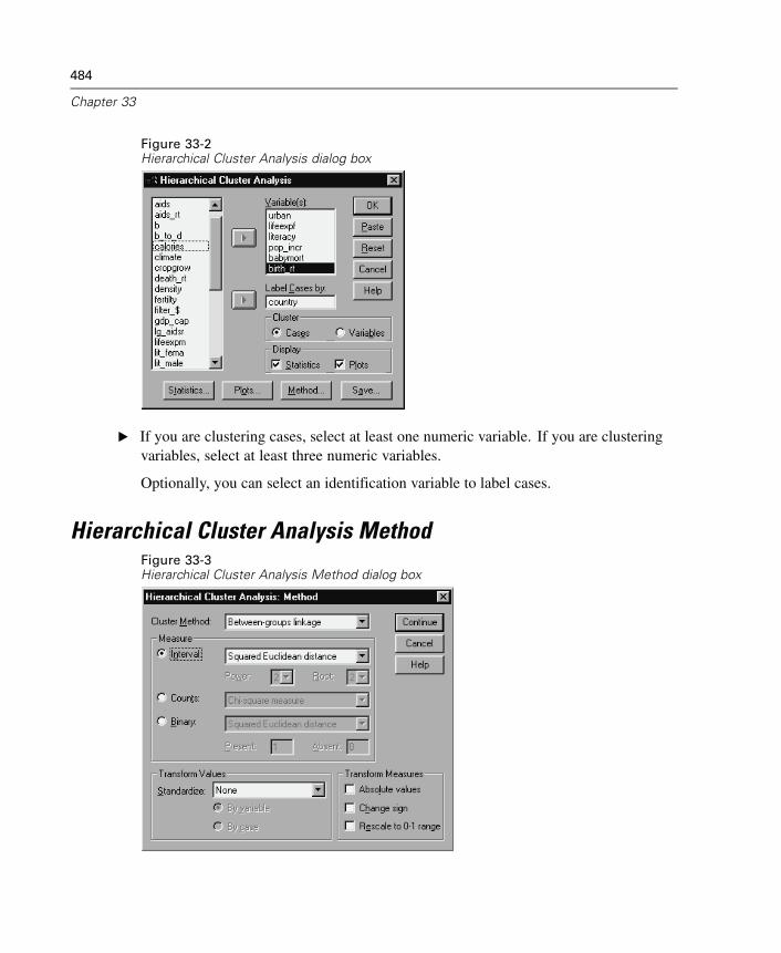
484

Chapter 33

Figure 33-2Hierarchical Cluster Analysis dialog box

E If you are clustering cases, select at least one numeric variable. If you are clusteringvariables, select at least three numeric variables.

Optionally, you can select an identification variable to label cases.

Hierarchical Cluster Analysis MethodFigure 33-3Hierarchical Cluster Analysis Method dialog box

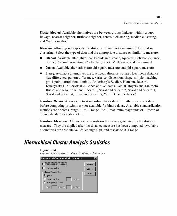
485


Cluster Method. Available alternatives are between-groups linkage, within-groupslinkage, nearest neighbor, furthest neighbor, centroid clustering, median clustering,and Ward’s method.

Measure. Allows you to specify the distance or similarity measure to be used inclustering. Select the type of data and the appropriate distance or similarity measure:

Interval. Available alternatives are Euclidean distance, squared Euclidean distance,cosine, Pearson correlation, Chebychev, block, Minkowski, and customized.

Counts. Available alternatives are chi-square measure and phi-square measure.

Binary. Available alternatives are Euclidean distance, squared Euclidean distance,size difference, pattern difference, variance, dispersion, shape, simple matching,phi 4-point correlation, lambda, Anderberg’s D, dice, Hamann, Jaccard,Kulczynski 1, Kulczynski 2, Lance and Williams, Ochiai, Rogers and Tanimoto,Russel and Rao, Sokal and Sneath 1, Sokal and Sneath 2, Sokal and Sneath 3,Sokal and Sneath 4, Sokal and Sneath 5, Yule’s Y, and Yule’s Q.

Transform Values. Allows you to standardize data values for either cases or valuesbefore computing proximities (not available for binary data). Available standardizationmethods are z scores, range –1 to 1, range 0 to 1, maximum magnitude of 1, mean of1, and standard deviation of 1.

Transform Measures. Allows you to transform the values generated by the distancemeasure. They are applied after the distance measure has been computed. Availablealternatives are absolute values, change sign, and rescale to 0–1 range.

Hierarchical Cluster Analysis StatisticsFigure 33-4Hierarchical Cluster Analysis Statistics dialog box

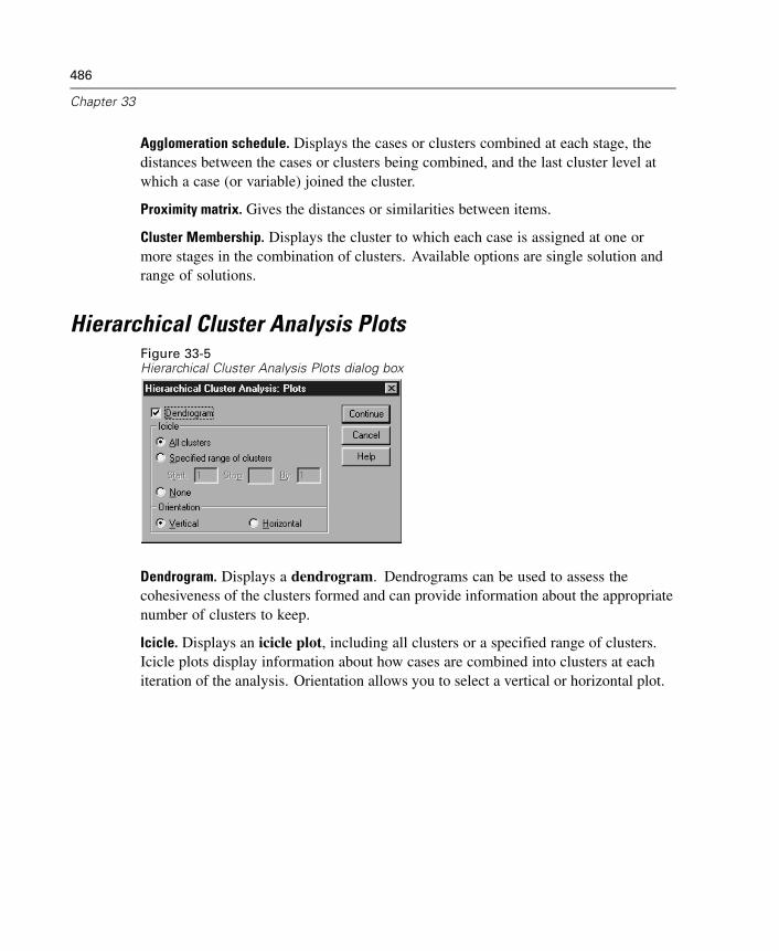
486

Chapter 33

Agglomeration schedule. Displays the cases or clusters combined at each stage, thedistances between the cases or clusters being combined, and the last cluster level atwhich a case (or variable) joined the cluster.

Proximity matrix. Gives the distances or similarities between items.

Cluster Membership. Displays the cluster to which each case is assigned at one ormore stages in the combination of clusters. Available options are single solution andrange of solutions.

Hierarchical Cluster Analysis PlotsFigure 33-5Hierarchical Cluster Analysis Plots dialog box

Dendrogram. Displays a dendrogram. Dendrograms can be used to assess thecohesiveness of the clusters formed and can provide information about the appropriatenumber of clusters to keep.

Icicle. Displays an icicle plot, including all clusters or a specified range of clusters.Icicle plots display information about how cases are combined into clusters at eachiteration of the analysis. Orientation allows you to select a vertical or horizontal plot.

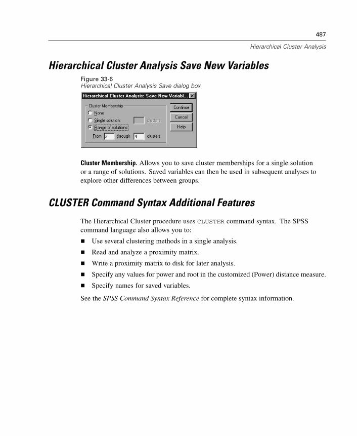
487


Hierarchical Cluster Analysis Save New VariablesFigure 33-6Hierarchical Cluster Analysis Save dialog box

Cluster Membership. Allows you to save cluster memberships for a single solutionor a range of solutions. Saved variables can then be used in subsequent analyses toexplore other differences between groups.

CLUSTER Command Syntax Additional Features

The Hierarchical Cluster procedure uses CLUSTER command syntax. The SPSScommand language also allows you to:

Use several clustering methods in a single analysis.

Read and analyze a proximity matrix.

Write a proximity matrix to disk for later analysis.

Specify any values for power and root in the customized (Power) distance measure.

Specify names for saved variables.


Chapter

34K-Means Cluster Analysis

This procedure attempts to identify relatively homogeneous groups of cases based onselected characteristics, using an algorithm that can handle large numbers of cases.However, the algorithm requires you to specify the number of clusters. You canspecify initial cluster centers if you know this information. You can select one of twomethods for classifying cases, either updating cluster centers iteratively or classifyingonly. You can save cluster membership, distance information, and final cluster centers.Optionally, you can specify a variable whose values are used to label casewise output.You can also request analysis of variance F statistics. While these statistics areopportunistic (the procedure tries to form groups that do differ), the relative size ofthe statistics provides information about each variable’s contribution to the separationof the groups.

Example. What are some identifiable groups of television shows that attract similaraudiences within each group? With k-means cluster analysis, you could clustertelevision shows (cases) into k homogeneous groups based on viewer characteristics.This process can be used to identify segments for marketing. Or you can clustercities (cases) into homogeneous groups so that comparable cities can be selected totest various marketing strategies.

Statistics. Complete solution: initial cluster centers, ANOVA table. Each case: clusterinformation, distance from cluster center.

Data. Variables should be quantitative at the interval or ratio level. If your variables arebinary or counts, use the Hierarchical Cluster Analysis procedure.

Case and initial cluster center order. The default algorithm for choosing initial clustercenters is not invariant to case ordering. The Use running means option on the Iteratedialog box makes the resulting solution potentially dependent on case order, regardlessof how initial cluster centers are chosen. If you are using either of these methods, youmay want to obtain several different solutions with cases sorted in different randomorders to verify the stability of a given solution. Specifying initial cluster centers and

489

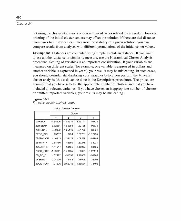
490

Chapter 34

not using the Use running means option will avoid issues related to case order. However,ordering of the initial cluster centers may affect the solution, if there are tied distancesfrom cases to cluster centers. To assess the stability of a given solution, you cancompare results from analyses with different permutations of the initial center values.

Assumptions. Distances are computed using simple Euclidean distance. If you wantto use another distance or similarity measure, use the Hierarchical Cluster Analysisprocedure. Scaling of variables is an important consideration. If your variables aremeasured on different scales (for example, one variable is expressed in dollars andanother variable is expressed in years), your results may be misleading. In such cases,you should consider standardizing your variables before you perform the k-meanscluster analysis (this task can be done in the Descriptives procedure). The procedureassumes that you have selected the appropriate number of clusters and that you haveincluded all relevant variables. If you have chosen an inappropriate number of clustersor omitted important variables, your results may be misleading.

Figure 34-1K-means cluster analysis output

-1.88606 -1.54314 1.45741 .55724

-3.52581 -1.69358 .62725 .99370

-2.89320 -1.65146 -.51770 .88601

.93737 .16291 3.03701 -1.12785

4.16813 1.38422 -.69589 -.88983

2.68796 .42699 .33278 -1.08033

4.41517 .63185 -1.89037 .63185

-1.99641 -1.78455 .53091 1.22118

-.52182 -.31333 4.40082 -.99285

2.24070 .75481 .46008 -.76793

.24626 2.65246 -1.29624 -.74406

ZURBAN

ZLIFEEXP

ZLITERAC

ZPOP_INC

ZBABYMOR

ZBIRTH_R

ZDEATH_R

ZLOG_GDP

ZB_TO_D

ZFERTILT

ZLOG_POP

1 2 3 4

Cluster

Initial Cluster Centers

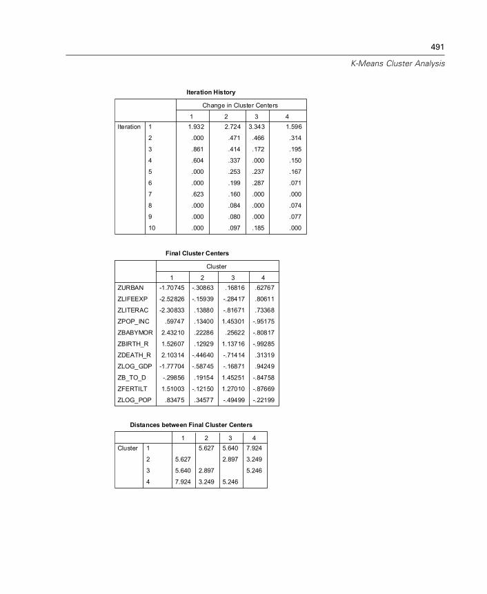
491

K-Means Cluster Analysis

1.932 2.724 3.343 1.596

.000 .471 .466 .314

.861 .414 .172 .195

.604 .337 .000 .150

.000 .253 .237 .167

.000 .199 .287 .071

.623 .160 .000 .000

.000 .084 .000 .074

.000 .080 .000 .077

.000 .097 .185 .000

1

2

3

4

5

6

7

8

9

10

Iteration1 2 3 4

Change in Cluster Centers

Iteration History

-1.70745 -.30863 .16816 .62767

-2.52826 -.15939 -.28417 .80611

-2.30833 .13880 -.81671 .73368

.59747 .13400 1.45301 -.95175

2.43210 .22286 .25622 -.80817

1.52607 .12929 1.13716 -.99285

2.10314 -.44640 -.71414 .31319

-1.77704 -.58745 -.16871 .94249

-.29856 .19154 1.45251 -.84758

1.51003 -.12150 1.27010 -.87669

.83475 .34577 -.49499 -.22199

ZURBAN

ZLIFEEXP

ZLITERAC

ZPOP_INC

ZBABYMOR

ZBIRTH_R

ZDEATH_R

ZLOG_GDP

ZB_TO_D

ZFERTILT

ZLOG_POP

1 2 3 4

Cluster

Final Cluster Centers

5.627 5.640 7.924

5.627 2.897 3.249

5.640 2.897 5.246

7.924 3.249 5.246

1

2

3

4

Cluster1 2 3 4

Distances between Final Cluster Centers

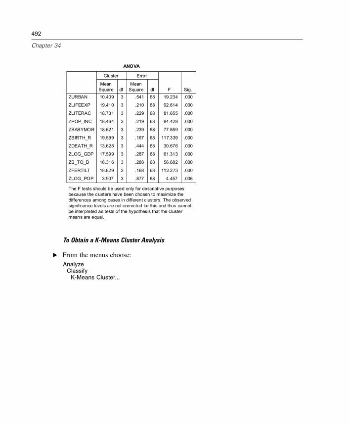
492

Chapter 34

10.409 3 .541 68 19.234 .000

19.410 3 .210 68 92.614 .000

18.731 3 .229 68 81.655 .000

18.464 3 .219 68 84.428 .000

18.621 3 .239 68 77.859 .000

19.599 3 .167 68 117.339 .000

13.628 3 .444 68 30.676 .000

17.599 3 .287 68 61.313 .000

16.316 3 .288 68 56.682 .000

18.829 3 .168 68 112.273 .000

3.907 3 .877 68 4.457 .006

ZURBAN

ZLIFEEXP

ZLITERAC

ZPOP_INC

ZBABYMOR

ZBIRTH_R

ZDEATH_R

ZLOG_GDP

ZB_TO_D

ZFERTILT

ZLOG_POP

MeanSquare df

Cluster

MeanSquare df

Error

F Sig.

ANOVA

The F tests should be used only for descriptive purposesbecause the clusters have been chosen to maximize thedifferences among cases in different clusters. The observedsignificance levels are not corrected for this and thus cannotbe interpreted as tests of the hypothesis that the clustermeans are equal.

To Obtain a K-Means Cluster Analysis


ClassifyK-Means Cluster...

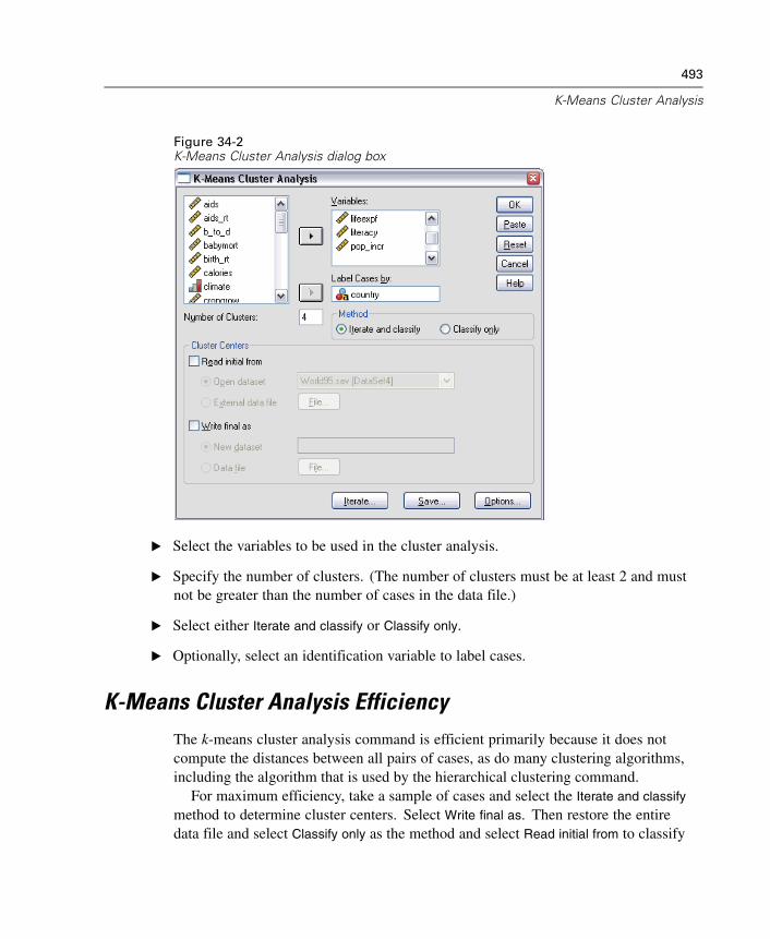
493


Figure 34-2K-Means Cluster Analysis dialog box

E Select the variables to be used in the cluster analysis.

E Specify the number of clusters. (The number of clusters must be at least 2 and mustnot be greater than the number of cases in the data file.)

E Select either Iterate and classify or Classify only.

E Optionally, select an identification variable to label cases.

K-Means Cluster Analysis EfficiencyThe k-means cluster analysis command is efficient primarily because it does notcompute the distances between all pairs of cases, as do many clustering algorithms,including the algorithm that is used by the hierarchical clustering command.

For maximum efficiency, take a sample of cases and select the Iterate and classify

method to determine cluster centers. Select Write final as. Then restore the entiredata file and select Classify only as the method and select Read initial from to classify

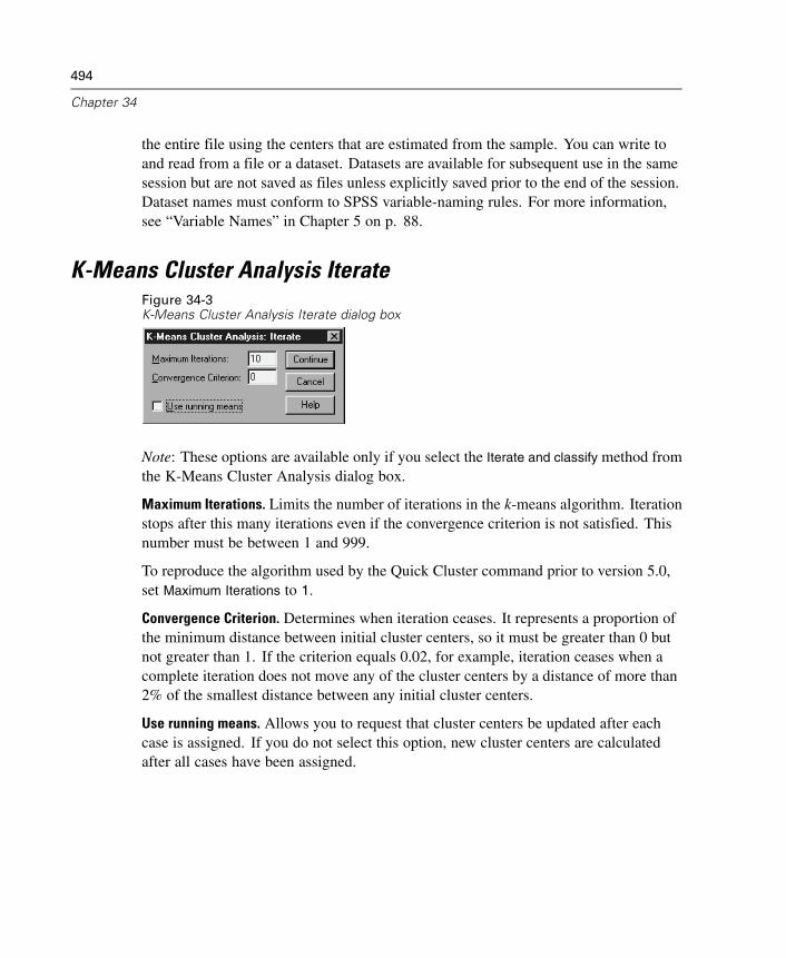
494

Chapter 34

the entire file using the centers that are estimated from the sample. You can write toand read from a file or a dataset. Datasets are available for subsequent use in the samesession but are not saved as files unless explicitly saved prior to the end of the session.Dataset names must conform to SPSS variable-naming rules. For more information,see “Variable Names” in Chapter 5 on p. 88.

K-Means Cluster Analysis IterateFigure 34-3K-Means Cluster Analysis Iterate dialog box

Note: These options are available only if you select the Iterate and classify method fromthe K-Means Cluster Analysis dialog box.

Maximum Iterations. Limits the number of iterations in the k-means algorithm. Iterationstops after this many iterations even if the convergence criterion is not satisfied. Thisnumber must be between 1 and 999.

To reproduce the algorithm used by the Quick Cluster command prior to version 5.0,set Maximum Iterations to 1.

Convergence Criterion. Determines when iteration ceases. It represents a proportion ofthe minimum distance between initial cluster centers, so it must be greater than 0 butnot greater than 1. If the criterion equals 0.02, for example, iteration ceases when acomplete iteration does not move any of the cluster centers by a distance of more than2% of the smallest distance between any initial cluster centers.

Use running means. Allows you to request that cluster centers be updated after eachcase is assigned. If you do not select this option, new cluster centers are calculatedafter all cases have been assigned.

495


K-Means Cluster Analysis SaveFigure 34-4K-Means Cluster Analysis Save New Variables dialog box

You can save information about the solution as new variables to be used in subsequentanalyses:

Cluster membership. Creates a new variable indicating the final cluster membership ofeach case. Values of the new variable range from 1 to the number of clusters.

Distance from cluster center. Creates a new variable indicating the Euclidean distancebetween each case and its classification center.

K-Means Cluster Analysis OptionsFigure 34-5K-Means Cluster Analysis Options dialog box

Statistics. You can select the following statistics: initial cluster centers, ANOVA table,and cluster information for each case.

Initial cluster centers. First estimate of the variable means for each of the clusters.By default, a number of well-spaced cases equal to the number of clustersis selected from the data. Initial cluster centers are used for a first round ofclassification and are then updated.

496

Chapter 34

ANOVA table. Displays an analysis-of-variance table which includes univariate Ftests for each clustering variable. The F tests are only descriptive and the resultingprobabilities should not be interpreted. The ANOVA table is not displayed if allcases are assigned to a single cluster.

Cluster information for each case. Displays for each case the final cluster assignmentand the Euclidean distance between the case and the cluster center used to classifythe case. Also displays Euclidean distance between final cluster centers.

Missing Values. Available options are Exclude cases listwise or Exclude cases pairwise.

Exclude cases listwise. Excludes cases with missing values for any clusteringvariable from the analysis.

Exclude cases pairwise. Assigns cases to clusters based on distances that arecomputed from all variables with nonmissing values.

QUICK CLUSTER Command Additional Features

The K-Means Cluster procedure uses QUICK CLUSTER command syntax. The SPSScommand language also allows you to:

Accept the first k cases as initial cluster centers, thereby avoiding the data passthat is normally used to estimate them.

Specify initial cluster centers directly as a part of the command syntax.

Specify names for saved variables.


Chapter

35Nonparametric Tests

The Nonparametric Tests procedure provides several tests that do not requireassumptions about the shape of the underlying distribution.

Chi-Square Test. Tabulates a variable into categories and computes a chi-square statisticbased on the differences between observed and expected frequencies.

Binomial Test. Compares the observed frequency in each category of a dichotomousvariable with expected frequencies from the binomial distribution.

Runs Test. Tests whether the order of occurrence of two values of a variable is random.

One-Sample Kolmogorov-Smirnov Test. Compares the observed cumulative distributionfunction for a variable with a specified theoretical distribution, which may be normal,uniform, exponential, or Poisson.

Two-Independent-Samples Tests. Compares two groups of cases on one variable. TheMann-Whitney U test, two-sample Kolmogorov-Smirnov test, Moses test of extremereactions, and Wald-Wolfowitz runs test are available.

Two-Related-Samples Tests. Compares the distributions of two variables. The Wilcoxonsigned-rank test, the sign test, and the McNemar test are available.

Tests for Several Independent Samples. Compares two or more groups of cases onone variable. The Kruskal-Wallis test, the Median test, and the Jonckheere-Terpstratest are available.

Tests for Several Related Samples. Compares the distributions of two or more variables.Friedman’s test, Kendall’s W, and Cochran’s Q are available.

Quartiles and the mean, standard deviation, minimum, maximum, and number ofnonmissing cases are available for all of the above tests.

497

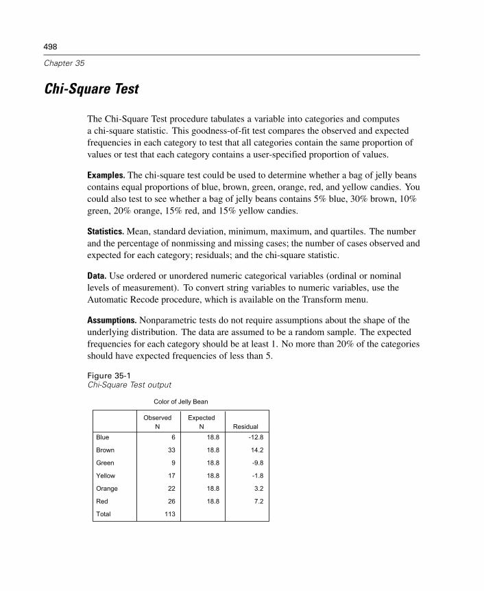
498

Chapter 35

Chi-Square Test

The Chi-Square Test procedure tabulates a variable into categories and computesa chi-square statistic. This goodness-of-fit test compares the observed and expectedfrequencies in each category to test that all categories contain the same proportion ofvalues or test that each category contains a user-specified proportion of values.

Examples. The chi-square test could be used to determine whether a bag of jelly beanscontains equal proportions of blue, brown, green, orange, red, and yellow candies. Youcould also test to see whether a bag of jelly beans contains 5% blue, 30% brown, 10%green, 20% orange, 15% red, and 15% yellow candies.

Statistics. Mean, standard deviation, minimum, maximum, and quartiles. The numberand the percentage of nonmissing and missing cases; the number of cases observed andexpected for each category; residuals; and the chi-square statistic.

Data. Use ordered or unordered numeric categorical variables (ordinal or nominallevels of measurement). To convert string variables to numeric variables, use theAutomatic Recode procedure, which is available on the Transform menu.

Assumptions. Nonparametric tests do not require assumptions about the shape of theunderlying distribution. The data are assumed to be a random sample. The expectedfrequencies for each category should be at least 1. No more than 20% of the categoriesshould have expected frequencies of less than 5.

Figure 35-1Chi-Square Test output

6 18.8 -12.8

33 18.8 14.2

9 18.8 -9.8

17 18.8 -1.8

22 18.8 3.2

26 18.8 7.2

113

Blue

Brown

Green

Yellow

Orange

Red

Total

ObservedN

ExpectedN Residual

Color of Jelly Bean

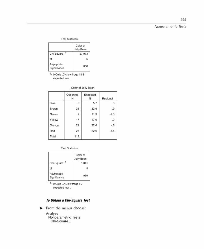
499

Nonparametric Tests

27.973

5

.000

Chi-Square 1

df

AsymptoticSignificance

Color ofJelly Bean

Test Statistics

0 Cells .0% low freqs 18.8expected low...

1.

6 5.7 .3

33 33.9 -.9

9 11.3 -2.3

17 17.0 .0

22 22.6 -.6

26 22.6 3.4

113

Blue

Brown

Green

Yellow

Orange

Red

Total

ObservedN

ExpectedN Residual

Color of Jelly Bean

1.041

5

.959

Chi-Square 1

df


Color ofJelly Bean

Test Statistics

0 Cells .0% low freqs 5.7expected low...

1.

To Obtain a Chi-Square Test


Nonparametric TestsChi-Square...

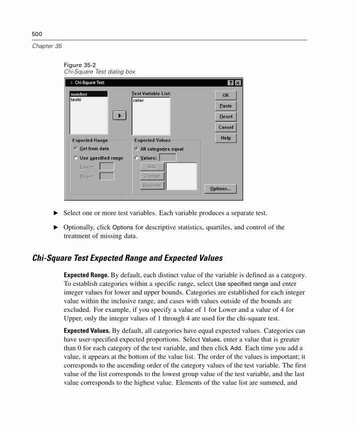
500

Chapter 35

Figure 35-2Chi-Square Test dialog box

E Select one or more test variables. Each variable produces a separate test.

E Optionally, click Options for descriptive statistics, quartiles, and control of thetreatment of missing data.

Chi-Square Test Expected Range and Expected Values

Expected Range. By default, each distinct value of the variable is defined as a category.To establish categories within a specific range, select Use specified range and enterinteger values for lower and upper bounds. Categories are established for each integervalue within the inclusive range, and cases with values outside of the bounds areexcluded. For example, if you specify a value of 1 for Lower and a value of 4 forUpper, only the integer values of 1 through 4 are used for the chi-square test.

Expected Values. By default, all categories have equal expected values. Categories canhave user-specified expected proportions. Select Values, enter a value that is greaterthan 0 for each category of the test variable, and then click Add. Each time you add avalue, it appears at the bottom of the value list. The order of the values is important; itcorresponds to the ascending order of the category values of the test variable. The firstvalue of the list corresponds to the lowest group value of the test variable, and the lastvalue corresponds to the highest value. Elements of the value list are summed, and

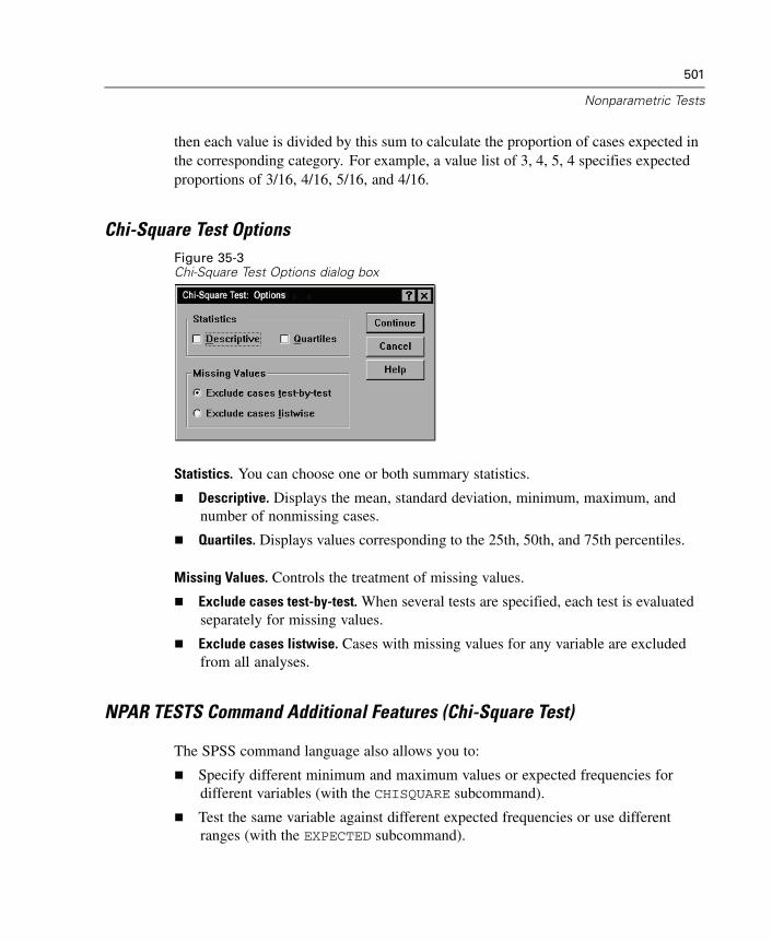
501

Nonparametric Tests

then each value is divided by this sum to calculate the proportion of cases expected inthe corresponding category. For example, a value list of 3, 4, 5, 4 specifies expectedproportions of 3/16, 4/16, 5/16, and 4/16.

Chi-Square Test OptionsFigure 35-3Chi-Square Test Options dialog box

Statistics. You can choose one or both summary statistics.

Descriptive. Displays the mean, standard deviation, minimum, maximum, andnumber of nonmissing cases.

Quartiles. Displays values corresponding to the 25th, 50th, and 75th percentiles.


Exclude cases test-by-test. When several tests are specified, each test is evaluatedseparately for missing values.

Exclude cases listwise. Cases with missing values for any variable are excludedfrom all analyses.

NPAR TESTS Command Additional Features (Chi-Square Test)


Specify different minimum and maximum values or expected frequencies fordifferent variables (with the CHISQUARE subcommand).

Test the same variable against different expected frequencies or use differentranges (with the EXPECTED subcommand).

502

Chapter 35


Binomial Test

The Binomial Test procedure compares the observed frequencies of the two categoriesof a dichotomous variable to the frequencies that are expected under a binomialdistribution with a specified probability parameter. By default, the probabilityparameter for both groups is 0.5. To change the probabilities, you can enter a testproportion for the first group. The probability for the second group will be 1 minus thespecified probability for the first group.

Example. When you toss a dime, the probability of a head equals 1/2. Based on thishypothesis, a dime is tossed 40 times, and the outcomes are recorded (heads or tails).From the binomial test, you might find that 3/4 of the tosses were heads and that theobserved significance level is small (0.0027). These results indicate that it is not likelythat the probability of a head equals 1/2; the coin is probably biased.

Statistics. Mean, standard deviation, minimum, maximum, number of nonmissingcases, and quartiles.

Data. The variables that are tested should be numeric and dichotomous. To convertstring variables to numeric variables, use the Automatic Recode procedure, which isavailable on the Transform menu. A dichotomous variable is a variable that can takeonly two possible values: yes or no, true or false, 0 or 1, and so on. If the variablesare not dichotomous, you must specify a cut point. The cut point assigns cases withvalues that are greater than the cut point to one group and assigns the rest of the casesto another group.

Assumptions. Nonparametric tests do not require assumptions about the shape of theunderlying distribution. The data are assumed to be a random sample.

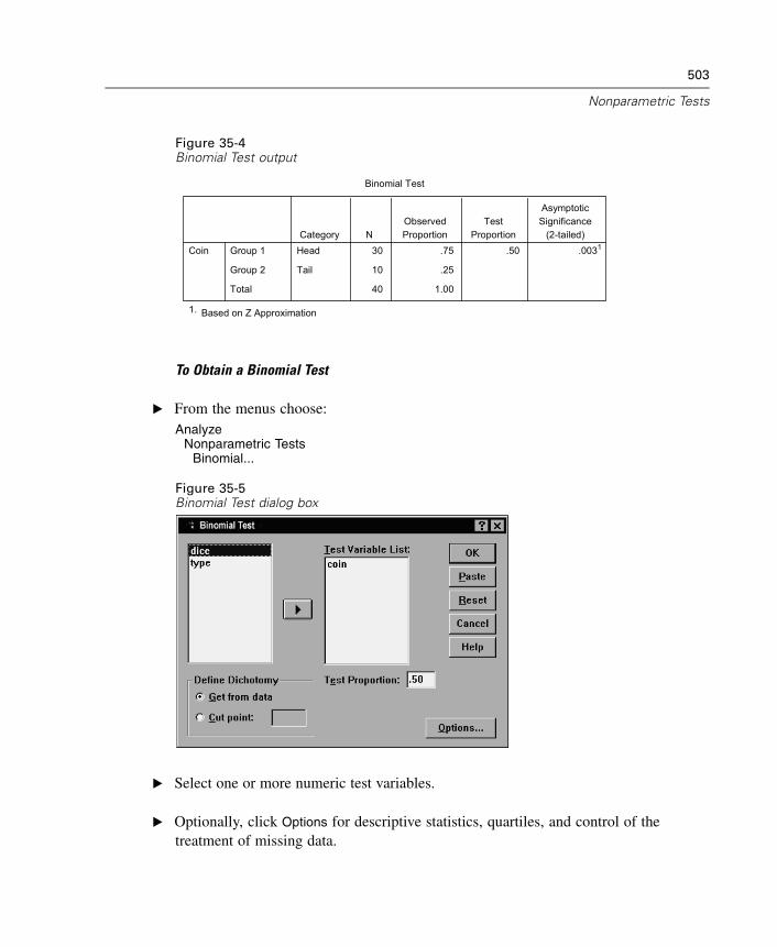
503

Nonparametric Tests

Figure 35-4Binomial Test output

Head 30 .75 .50 .0031

Tail 10 .25

40 1.00

Group 1

Group 2

Total

CoinCategory N

ObservedProportion

TestProportion


(2-tailed)

Binomial Test

Based on Z Approximation1.

To Obtain a Binomial Test


Nonparametric TestsBinomial...

Figure 35-5Binomial Test dialog box

E Select one or more numeric test variables.


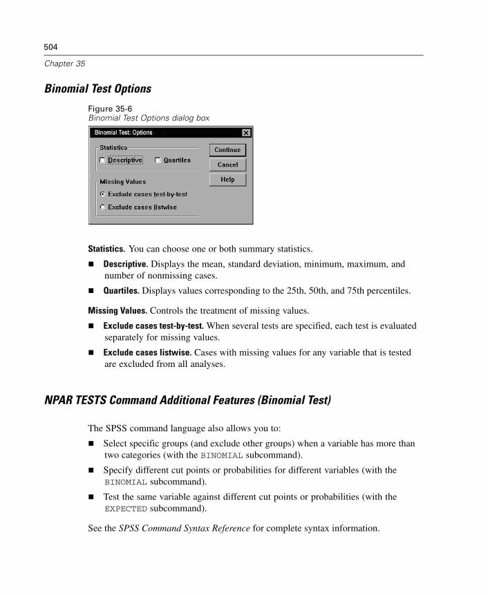
504

Chapter 35

Binomial Test Options

Figure 35-6Binomial Test Options dialog box






Exclude cases listwise. Cases with missing values for any variable that is testedare excluded from all analyses.

NPAR TESTS Command Additional Features (Binomial Test)


Select specific groups (and exclude other groups) when a variable has more thantwo categories (with the BINOMIAL subcommand).

Specify different cut points or probabilities for different variables (with theBINOMIAL subcommand).

Test the same variable against different cut points or probabilities (with theEXPECTED subcommand).


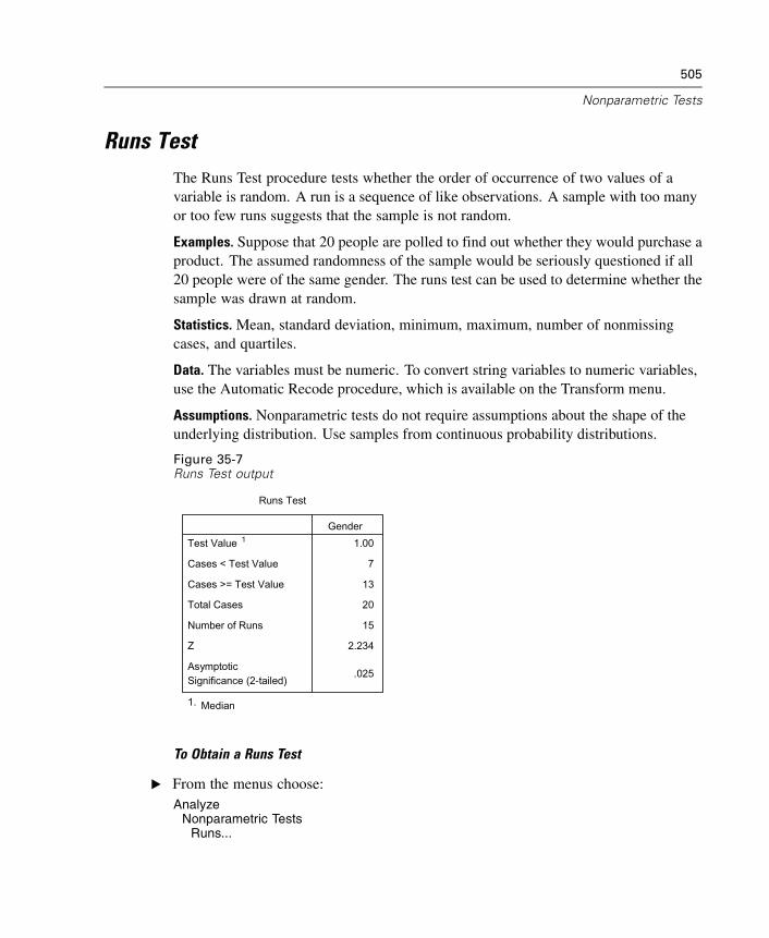
505

Nonparametric Tests

Runs TestThe Runs Test procedure tests whether the order of occurrence of two values of avariable is random. A run is a sequence of like observations. A sample with too manyor too few runs suggests that the sample is not random.

Examples. Suppose that 20 people are polled to find out whether they would purchase aproduct. The assumed randomness of the sample would be seriously questioned if all20 people were of the same gender. The runs test can be used to determine whether thesample was drawn at random.


Data. The variables must be numeric. To convert string variables to numeric variables,use the Automatic Recode procedure, which is available on the Transform menu.

Assumptions. Nonparametric tests do not require assumptions about the shape of theunderlying distribution. Use samples from continuous probability distributions.

Figure 35-7Runs Test output

1.00

7

13

20

15

2.234

.025

Test Value 1

Cases < Test Value

Cases >= Test Value

Total Cases

Number of Runs

Z

AsymptoticSignificance (2-tailed)

Gender

Runs Test

Median1.

To Obtain a Runs Test


Nonparametric TestsRuns...

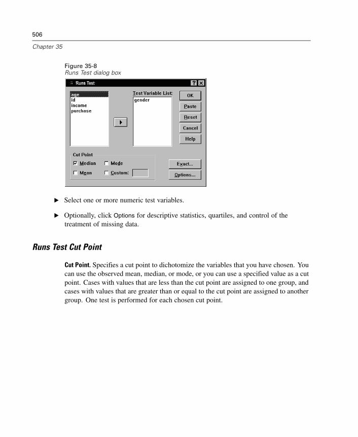
506

Chapter 35

Figure 35-8Runs Test dialog box

E Select one or more numeric test variables.


Runs Test Cut Point

Cut Point. Specifies a cut point to dichotomize the variables that you have chosen. Youcan use the observed mean, median, or mode, or you can use a specified value as a cutpoint. Cases with values that are less than the cut point are assigned to one group, andcases with values that are greater than or equal to the cut point are assigned to anothergroup. One test is performed for each chosen cut point.

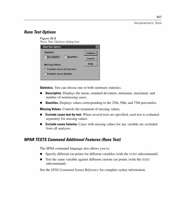
507

Nonparametric Tests

Runs Test OptionsFigure 35-9Runs Test Options dialog box







NPAR TESTS Command Additional Features (Runs Test)


Specify different cut points for different variables (with the RUNS subcommand).

Test the same variable against different custom cut points (with the RUNSsubcommand).


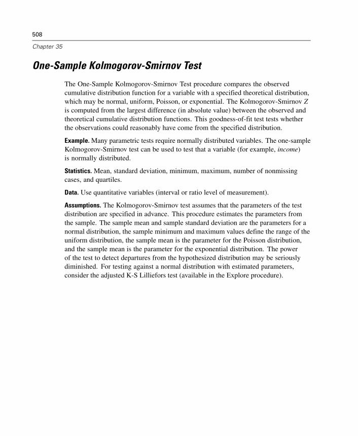
508

Chapter 35

One-Sample Kolmogorov-Smirnov Test

The One-Sample Kolmogorov-Smirnov Test procedure compares the observedcumulative distribution function for a variable with a specified theoretical distribution,which may be normal, uniform, Poisson, or exponential. The Kolmogorov-Smirnov Zis computed from the largest difference (in absolute value) between the observed andtheoretical cumulative distribution functions. This goodness-of-fit test tests whetherthe observations could reasonably have come from the specified distribution.

Example. Many parametric tests require normally distributed variables. The one-sampleKolmogorov-Smirnov test can be used to test that a variable (for example, income)is normally distributed.


Data. Use quantitative variables (interval or ratio level of measurement).

Assumptions. The Kolmogorov-Smirnov test assumes that the parameters of the testdistribution are specified in advance. This procedure estimates the parameters fromthe sample. The sample mean and sample standard deviation are the parameters for anormal distribution, the sample minimum and maximum values define the range of theuniform distribution, the sample mean is the parameter for the Poisson distribution,and the sample mean is the parameter for the exponential distribution. The powerof the test to detect departures from the hypothesized distribution may be seriouslydiminished. For testing against a normal distribution with estimated parameters,consider the adjusted K-S Lilliefors test (available in the Explore procedure).

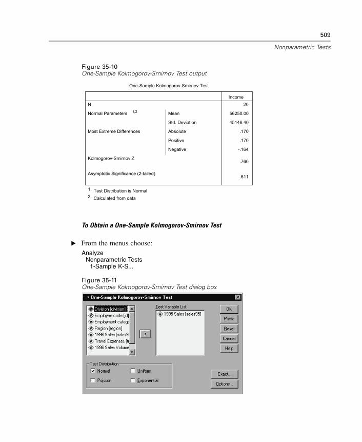
509

Nonparametric Tests

Figure 35-10One-Sample Kolmogorov-Smirnov Test output

20

56250.00

45146.40

.170

.170

-.164

.760

.611

N

Mean

Std. Deviation

Normal Parameters 1,2

Absolute

Positive

Negative

Most Extreme Differences

Kolmogorov-Smirnov Z

Asymptotic Significance (2-tailed)

Income

One-Sample Kolmogorov-Smirnov Test

Test Distribution is Normal1.

Calculated from data2.

To Obtain a One-Sample Kolmogorov-Smirnov Test


Nonparametric Tests1-Sample K-S...

Figure 35-11One-Sample Kolmogorov-Smirnov Test dialog box

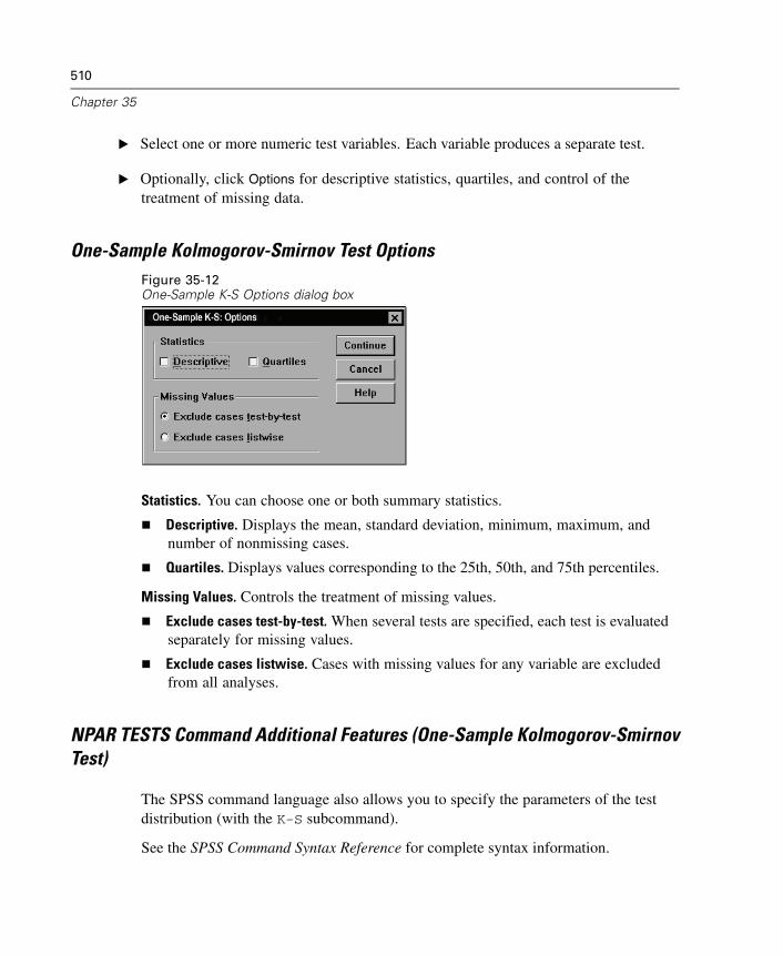
510

Chapter 35

E Select one or more numeric test variables. Each variable produces a separate test.


One-Sample Kolmogorov-Smirnov Test OptionsFigure 35-12One-Sample K-S Options dialog box







NPAR TESTS Command Additional Features (One-Sample Kolmogorov-SmirnovTest)

The SPSS command language also allows you to specify the parameters of the testdistribution (with the K-S subcommand).


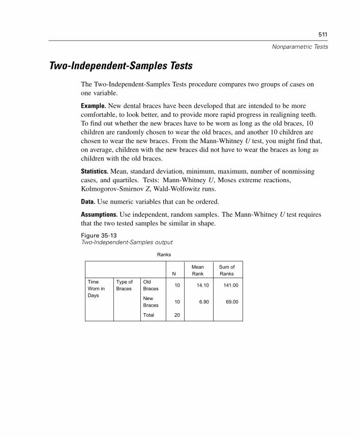
511

Nonparametric Tests

Two-Independent-Samples Tests

The Two-Independent-Samples Tests procedure compares two groups of cases onone variable.

Example. New dental braces have been developed that are intended to be morecomfortable, to look better, and to provide more rapid progress in realigning teeth.To find out whether the new braces have to be worn as long as the old braces, 10children are randomly chosen to wear the old braces, and another 10 children arechosen to wear the new braces. From the Mann-Whitney U test, you might find that,on average, children with the new braces did not have to wear the braces as long aschildren with the old braces.

Statistics. Mean, standard deviation, minimum, maximum, number of nonmissingcases, and quartiles. Tests: Mann-Whitney U, Moses extreme reactions,Kolmogorov-Smirnov Z, Wald-Wolfowitz runs.

Data. Use numeric variables that can be ordered.

Assumptions. Use independent, random samples. The Mann-Whitney U test requiresthat the two tested samples be similar in shape.

Figure 35-13Two-Independent-Samples output

10 14.10 141.00

10 6.90 69.00

20

OldBraces

NewBraces

Total

Type ofBraces

TimeWorn inDays

NMeanRank

Sum ofRanks

Ranks

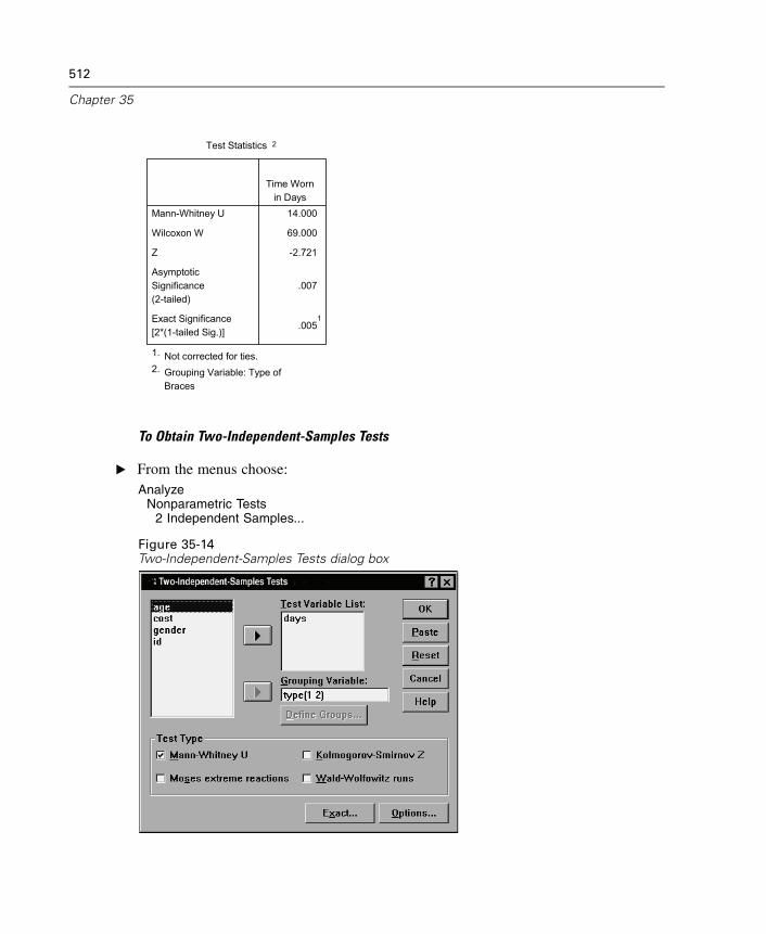
512

Chapter 35

14.000

69.000

-2.721

.007

.0051

Mann-Whitney U

Wilcoxon W

Z

AsymptoticSignificance(2-tailed)

Exact Significance[2*(1-tailed Sig.)]

Time Wornin Days

Test Statistics 2

Not corrected for ties.1.

Grouping Variable: Type ofBraces

2.

To Obtain Two-Independent-Samples Tests


Nonparametric Tests2 Independent Samples...

Figure 35-14Two-Independent-Samples Tests dialog box

513

Nonparametric Tests

E Select one or more numeric variables.

E Select a grouping variable and click Define Groups to split the file into two groups orsamples.

Two-Independent-Samples Test Types

Test Type. Four tests are available to test whether two independent samples (groups)come from the same population.

The Mann-Whitney U test is the most popular of the two-independent-samplestests. It is equivalent to the Wilcoxon rank sum test and the Kruskal-Wallis test for twogroups. Mann-Whitney tests that two sampled populations are equivalent in location.The observations from both groups are combined and ranked, with the average rankassigned in the case of ties. The number of ties should be small relative to the totalnumber of observations. If the populations are identical in location, the ranks shouldbe randomly mixed between the two samples. The test calculates the number oftimes that a score from group 1 precedes a score from group 2 and the number oftimes that a score from group 2 precedes a score from group 1. The Mann-WhitneyU statistic is the smaller of these two numbers. The Wilcoxon rank sum W statistic,also displayed, is the rank sum of the smaller sample. If both samples have the samenumber of observations, W is the rank sum of the group that is named first in theTwo-Independent-Samples Define Groups dialog box.

The Kolmogorov-Smirnov Z test and the Wald-Wolfowitz runs test are moregeneral tests that detect differences in both the locations and shapes of the distributions.The Kolmogorov-Smirnov test is based on the maximum absolute differencebetween the observed cumulative distribution functions for both samples. When thisdifference is significantly large, the two distributions are considered different. TheWald-Wolfowitz runs test combines and ranks the observations from both groups. Ifthe two samples are from the same population, the two groups should be randomlyscattered throughout the ranking.

The Moses extreme reactions test assumes that the experimental variable willaffect some subjects in one direction and other subjects in the opposite direction.The test tests for extreme responses compared to a control group. This test focuseson the span of the control group and is a measure of how much extreme values in theexperimental group influence the span when combined with the control group. Thecontrol group is defined by the group 1 value in the Two-Independent-Samples DefineGroups dialog box. Observations from both groups are combined and ranked. The span

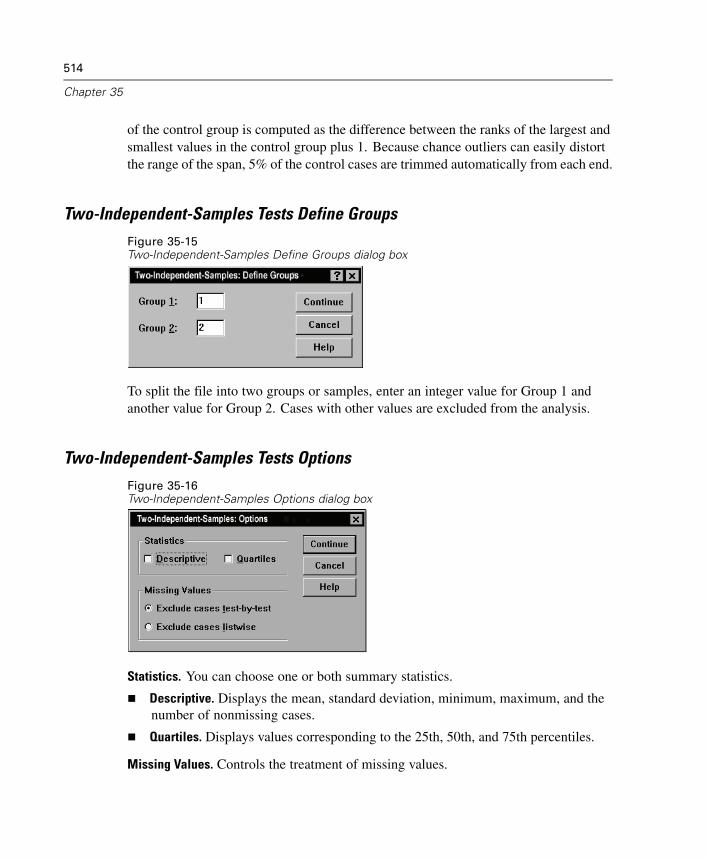
514

Chapter 35

of the control group is computed as the difference between the ranks of the largest andsmallest values in the control group plus 1. Because chance outliers can easily distortthe range of the span, 5% of the control cases are trimmed automatically from each end.

Two-Independent-Samples Tests Define GroupsFigure 35-15Two-Independent-Samples Define Groups dialog box

To split the file into two groups or samples, enter an integer value for Group 1 andanother value for Group 2. Cases with other values are excluded from the analysis.

Two-Independent-Samples Tests OptionsFigure 35-16Two-Independent-Samples Options dialog box


Descriptive. Displays the mean, standard deviation, minimum, maximum, and thenumber of nonmissing cases.



515

Nonparametric Tests



NPAR TESTS Command Additional Features (Two-Independent-Samples Tests)

The SPSS command language also allows you to specify the number of cases to betrimmed for the Moses test (with the MOSES subcommand).


Two-Related-Samples Tests

The Two-Related-Samples Tests procedure compares the distributions of two variables.

Example. In general, do families receive the asking price when they sell their homes?By applying the Wilcoxon signed-rank test to data for 10 homes, you might learn thatseven families receive less than the asking price, one family receives more than theasking price, and two families receive the asking price.

Statistics. Mean, standard deviation, minimum, maximum, number of nonmissingcases, and quartiles. Tests: Wilcoxon signed-rank, sign, McNemar.


Assumptions. Although no particular distributions are assumed for the two variables,the population distribution of the paired differences is assumed to be symmetric.

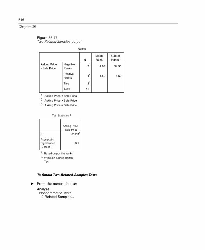
516

Chapter 35

Figure 35-17Two-Related-Samples output

71

4.93 34.50

12

1.50 1.50

23

10

NegativeRanks

PositiveRanks

Ties

Total

Asking Price- Sale Price

NMeanRank

Sum ofRanks

Ranks

Asking Price < Sale Price1.

Asking Price > Sale Price2.

Asking Price = Sale Price3.

-2.3131

.021

Z

AsymptoticSignificance(2-tailed)

Asking Price- Sale Price

Test Statistics 2

Based on positive ranks1.

Wilcoxon Signed RanksTest

2.

To Obtain Two-Related-Samples Tests


Nonparametric Tests2 Related Samples...

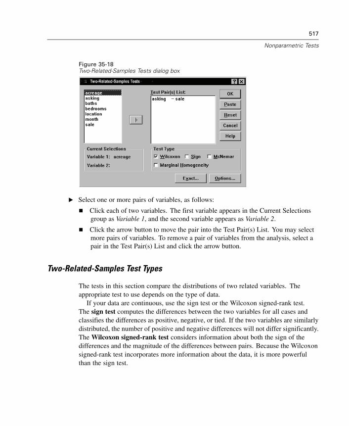
517

Nonparametric Tests

Figure 35-18Two-Related-Samples Tests dialog box

E Select one or more pairs of variables, as follows:

Click each of two variables. The first variable appears in the Current Selectionsgroup as Variable 1, and the second variable appears as Variable 2.

Click the arrow button to move the pair into the Test Pair(s) List. You may selectmore pairs of variables. To remove a pair of variables from the analysis, select apair in the Test Pair(s) List and click the arrow button.

Two-Related-Samples Test Types

The tests in this section compare the distributions of two related variables. Theappropriate test to use depends on the type of data.

If your data are continuous, use the sign test or the Wilcoxon signed-rank test.The sign test computes the differences between the two variables for all cases andclassifies the differences as positive, negative, or tied. If the two variables are similarlydistributed, the number of positive and negative differences will not differ significantly.The Wilcoxon signed-rank test considers information about both the sign of thedifferences and the magnitude of the differences between pairs. Because the Wilcoxonsigned-rank test incorporates more information about the data, it is more powerfulthan the sign test.

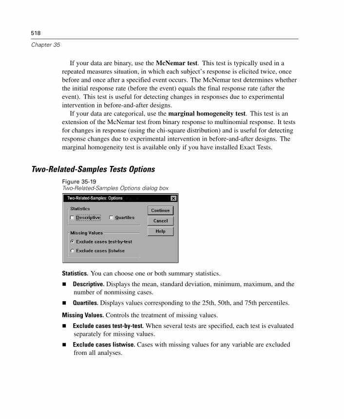
518

Chapter 35

If your data are binary, use the McNemar test. This test is typically used in arepeated measures situation, in which each subject’s response is elicited twice, oncebefore and once after a specified event occurs. The McNemar test determines whetherthe initial response rate (before the event) equals the final response rate (after theevent). This test is useful for detecting changes in responses due to experimentalintervention in before-and-after designs.

If your data are categorical, use the marginal homogeneity test. This test is anextension of the McNemar test from binary response to multinomial response. It testsfor changes in response (using the chi-square distribution) and is useful for detectingresponse changes due to experimental intervention in before-and-after designs. Themarginal homogeneity test is available only if you have installed Exact Tests.

Two-Related-Samples Tests OptionsFigure 35-19Two-Related-Samples Options dialog box







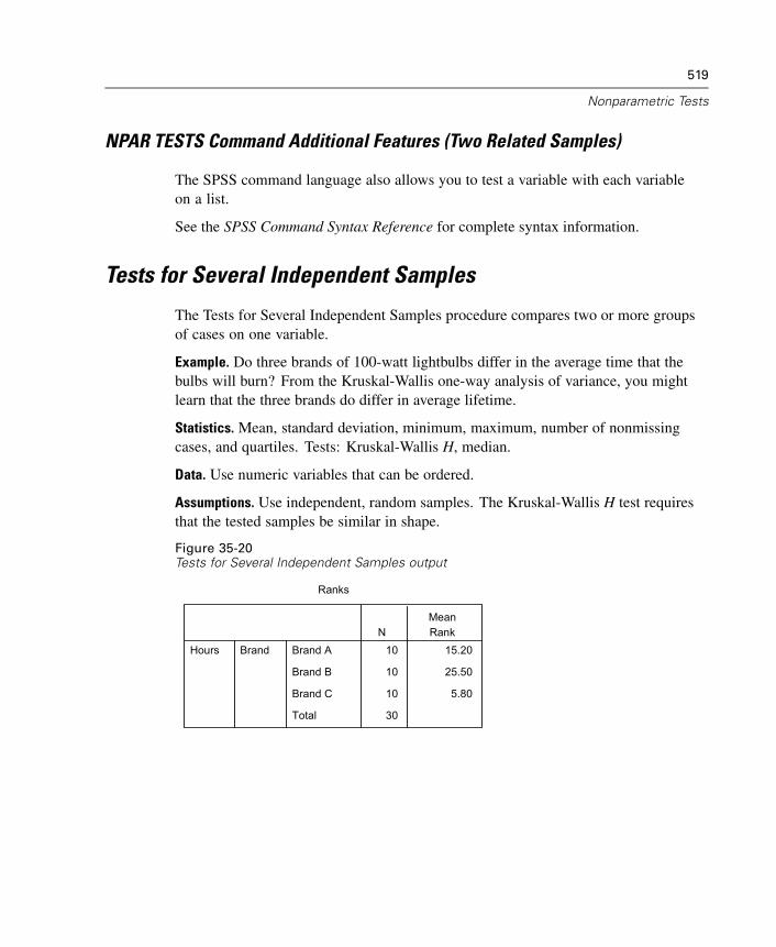
519

Nonparametric Tests

NPAR TESTS Command Additional Features (Two Related Samples)

The SPSS command language also allows you to test a variable with each variableon a list.


Tests for Several Independent Samples

The Tests for Several Independent Samples procedure compares two or more groupsof cases on one variable.

Example. Do three brands of 100-watt lightbulbs differ in the average time that thebulbs will burn? From the Kruskal-Wallis one-way analysis of variance, you mightlearn that the three brands do differ in average lifetime.

Statistics. Mean, standard deviation, minimum, maximum, number of nonmissingcases, and quartiles. Tests: Kruskal-Wallis H, median.


Assumptions. Use independent, random samples. The Kruskal-Wallis H test requiresthat the tested samples be similar in shape.

Figure 35-20Tests for Several Independent Samples output

10 15.20

10 25.50

10 5.80

30

Brand A

Brand B

Brand C

Total

BrandHoursN

MeanRank

Ranks

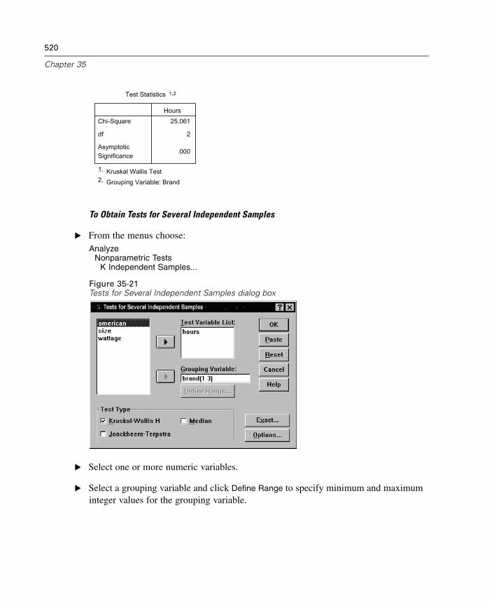
520

Chapter 35

25.061

2

.000

Chi-Square

df


Hours

Test Statistics 1,2

Kruskal Wallis Test1.

Grouping Variable: Brand2.

To Obtain Tests for Several Independent Samples


Nonparametric TestsK Independent Samples...

Figure 35-21Tests for Several Independent Samples dialog box

E Select one or more numeric variables.

E Select a grouping variable and click Define Range to specify minimum and maximuminteger values for the grouping variable.

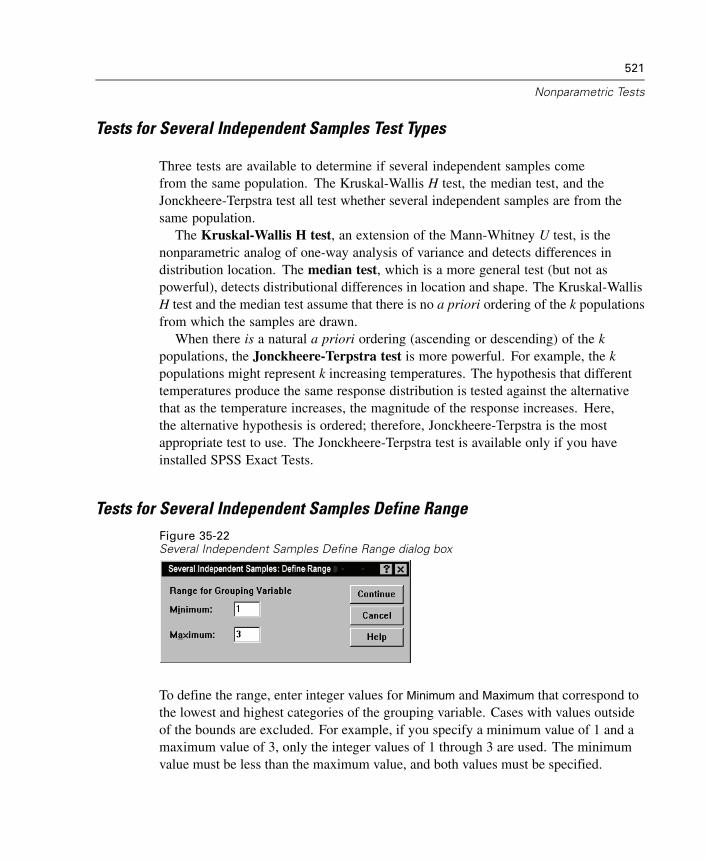
521

Nonparametric Tests

Tests for Several Independent Samples Test Types

Three tests are available to determine if several independent samples comefrom the same population. The Kruskal-Wallis H test, the median test, and theJonckheere-Terpstra test all test whether several independent samples are from thesame population.

The Kruskal-Wallis H test, an extension of the Mann-Whitney U test, is thenonparametric analog of one-way analysis of variance and detects differences indistribution location. The median test, which is a more general test (but not aspowerful), detects distributional differences in location and shape. The Kruskal-WallisH test and the median test assume that there is no a priori ordering of the k populationsfrom which the samples are drawn.

When there is a natural a priori ordering (ascending or descending) of the kpopulations, the Jonckheere-Terpstra test is more powerful. For example, the kpopulations might represent k increasing temperatures. The hypothesis that differenttemperatures produce the same response distribution is tested against the alternativethat as the temperature increases, the magnitude of the response increases. Here,the alternative hypothesis is ordered; therefore, Jonckheere-Terpstra is the mostappropriate test to use. The Jonckheere-Terpstra test is available only if you haveinstalled SPSS Exact Tests.

Tests for Several Independent Samples Define RangeFigure 35-22Several Independent Samples Define Range dialog box

To define the range, enter integer values for Minimum and Maximum that correspond tothe lowest and highest categories of the grouping variable. Cases with values outsideof the bounds are excluded. For example, if you specify a minimum value of 1 and amaximum value of 3, only the integer values of 1 through 3 are used. The minimumvalue must be less than the maximum value, and both values must be specified.

522

Chapter 35

Tests for Several Independent Samples Options

Figure 35-23Several Independent Samples Options dialog box







NPAR TESTS Command Additional Features (K Independent Samples)

The SPSS command language also allows you to specify a value other than theobserved median for the median test (with the MEDIAN subcommand).


Tests for Several Related Samples

The Tests for Several Related Samples procedure compares the distributions of twoor more variables.

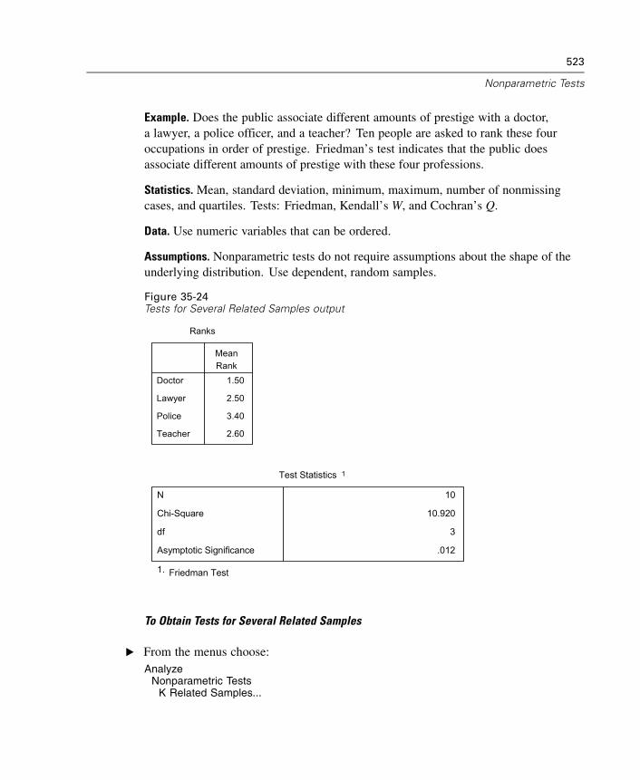
523

Nonparametric Tests

Example. Does the public associate different amounts of prestige with a doctor,a lawyer, a police officer, and a teacher? Ten people are asked to rank these fouroccupations in order of prestige. Friedman’s test indicates that the public doesassociate different amounts of prestige with these four professions.

Statistics. Mean, standard deviation, minimum, maximum, number of nonmissingcases, and quartiles. Tests: Friedman, Kendall’s W, and Cochran’s Q.


Assumptions. Nonparametric tests do not require assumptions about the shape of theunderlying distribution. Use dependent, random samples.

Figure 35-24Tests for Several Related Samples output

1.50

2.50

3.40

2.60

Doctor

Lawyer

Police

Teacher

MeanRank

Ranks

10

10.920

3

.012

N

Chi-Square

df

Asymptotic Significance

Test Statistics 1

Friedman Test1.

To Obtain Tests for Several Related Samples


Nonparametric TestsK Related Samples...

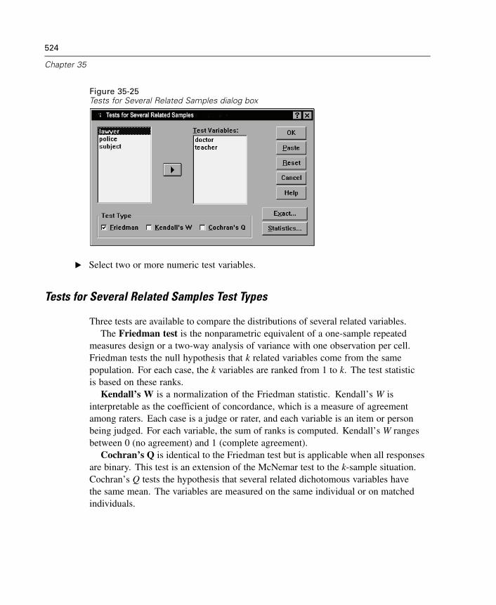
524

Chapter 35

Figure 35-25Tests for Several Related Samples dialog box

E Select two or more numeric test variables.

Tests for Several Related Samples Test Types

Three tests are available to compare the distributions of several related variables.The Friedman test is the nonparametric equivalent of a one-sample repeated

measures design or a two-way analysis of variance with one observation per cell.Friedman tests the null hypothesis that k related variables come from the samepopulation. For each case, the k variables are ranked from 1 to k. The test statisticis based on these ranks.

Kendall’s W is a normalization of the Friedman statistic. Kendall’s W isinterpretable as the coefficient of concordance, which is a measure of agreementamong raters. Each case is a judge or rater, and each variable is an item or personbeing judged. For each variable, the sum of ranks is computed. Kendall’s W rangesbetween 0 (no agreement) and 1 (complete agreement).

Cochran’s Q is identical to the Friedman test but is applicable when all responsesare binary. This test is an extension of the McNemar test to the k-sample situation.Cochran’s Q tests the hypothesis that several related dichotomous variables havethe same mean. The variables are measured on the same individual or on matchedindividuals.

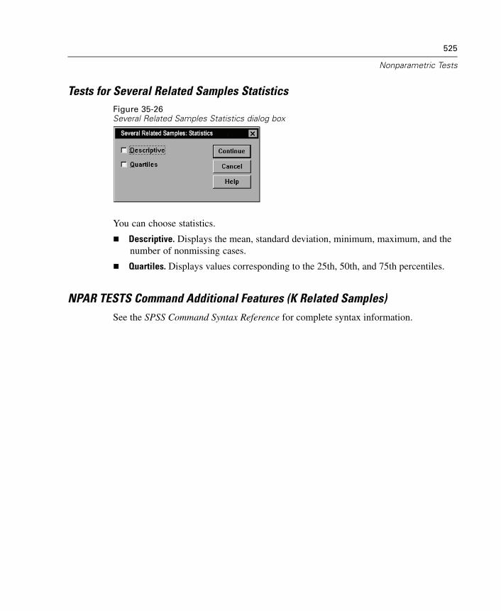
525

Nonparametric Tests

Tests for Several Related Samples StatisticsFigure 35-26Several Related Samples Statistics dialog box

You can choose statistics.



NPAR TESTS Command Additional Features (K Related Samples)See the SPSS Command Syntax Reference for complete syntax information.

Chapter

36Multiple Response Analysis

Two procedures are available for analyzing multiple dichotomy and multiple categorysets. The Multiple Response Frequencies procedure displays frequency tables.The Multiple Response Crosstabs procedure displays two- and three-dimensionalcrosstabulations. Before using either procedure, you must define multiple responsesets.

Example. This example illustrates the use of multiple response items in a marketresearch survey. The data are fictitious and should not be interpreted as real. An airlinemight survey passengers flying a particular route to evaluate competing carriers. In thisexample, American Airlines wants to know about its passengers’ use of other airlineson the Chicago-New York route and the relative importance of schedule and service inselecting an airline. The flight attendant hands each passenger a brief questionnaireupon boarding. The first question reads: Circle all airlines you have flown at least oncein the last six months on this route—American, United, TWA, USAir, Other. This isa multiple response question, since the passenger can circle more than one response.However, this question cannot be coded directly because a variable can have onlyone value for each case. You must use several variables to map responses to eachquestion. There are two ways to do this. One is to define a variable corresponding toeach of the choices (for example, American, United, TWA, USAir, and Other). If thepassenger circles United, the variable united is assigned a code of 1, otherwise 0.This is a multiple dichotomy method of mapping variables. The other way to mapresponses is the multiple category method, in which you estimate the maximumnumber of possible responses to the question and set up the same number of variables,with codes used to specify the airline flown. By perusing a sample of questionnaires,you might discover that no user has flown more than three different airlines on thisroute in the last six months. Further, you find that due to the deregulation of airlines,10 other airlines are named in the Other category. Using the multiple response method,you would define three variables, each coded as 1 = american, 2 = united, 3 = twa, 4 =usair, 5 = delta, and so on. If a given passenger circles American and TWA, the first

527

528

Chapter 36

variable has a code of 1, the second has a code of 3, and the third has a missing-valuecode. Another passenger might have circled American and entered Delta. Thus, thefirst variable has a code of 1, the second has a code of 5, and the third a missing-valuecode. If you use the multiple dichotomy method, on the other hand, you end up with14 separate variables. Although either method of mapping is feasible for this survey,the method you choose depends on the distribution of responses.

Multiple Response Define SetsThe Define Multiple Response Sets procedure groups elementary variables intomultiple dichotomy and multiple category sets, for which you can obtain frequencytables and crosstabulations. You can define up to 20 multiple response sets. Eachset must have a unique name. To remove a set, highlight it on the list of multipleresponse sets and click Remove. To change a set, highlight it on the list, modify any setdefinition characteristics, and click Change.

You can code your elementary variables as dichotomies or categories. To usedichotomous variables, select Dichotomies to create a multiple dichotomy set. Enter aninteger value for Counted value. Each variable having at least one occurrence of thecounted value becomes a category of the multiple dichotomy set. Select Categories

to create a multiple category set having the same range of values as the componentvariables. Enter integer values for the minimum and maximum values of the range forcategories of the multiple category set. The procedure totals each distinct integervalue in the inclusive range across all component variables. Empty categories arenot tabulated.

Each multiple response set must be assigned a unique name of up to sevencharacters. The procedure prefixes a dollar sign ($) to the name you assign. You cannotuse the following reserved names: casenum, sysmis, jdate, date, time, length, andwidth. The name of the multiple response set exists only for use in multiple responseprocedures. You cannot refer to multiple response set names in other procedures.Optionally, you can enter a descriptive variable label for the multiple response set.The label can be up to 40 characters long.

To Define Multiple Response Sets


Multiple ResponseDefine Sets...

529

Multiple Response Analysis

Figure 36-1Define Multiple Response Sets dialog box

E Select two or more variables.

E If your variables are coded as dichotomies, indicate which value you want to havecounted. If your variables are coded as categories, define the range of the categories.

E Enter a unique name for each multiple response set.

E Click Add to add the multiple response set to the list of defined sets.

Multiple Response Frequencies

The Multiple Response Frequencies procedure produces frequency tables for multipleresponse sets. You must first define one or more multiple response sets (see “MultipleResponse Define Sets”).

For multiple dichotomy sets, category names shown in the output come fromvariable labels defined for elementary variables in the group. If the variable labels arenot defined, variable names are used as labels. For multiple category sets, categorylabels come from the value labels of the first variable in the group. If categoriesmissing for the first variable are present for other variables in the group, define avalue label for the missing categories.

530

Chapter 36

Missing Values. Cases with missing values are excluded on a table-by-table basis.Alternatively, you can choose one or both of the following:

Exclude cases listwise within dichotomies. Excludes cases with missing valuesfor any variable from the tabulation of the multiple dichotomy set. This appliesonly to multiple response sets defined as dichotomy sets. By default, a caseis considered missing for a multiple dichotomy set if none of its componentvariables contains the counted value. Cases with missing values for some (but notall variables) are included in the tabulations of the group if at least one variablecontains the counted value.

Exclude cases listwise within categories. Excludes cases with missing values forany variable from tabulation of the multiple category set. This applies only tomultiple response sets defined as category sets. By default, a case is consideredmissing for a multiple category set only if none of its components has valid valueswithin the defined range.

Example. Each variable created from a survey question is an elementary variable. Toanalyze a multiple response item, you must combine the variables into one of twotypes of multiple response sets: a multiple dichotomy set or a multiple category set.For example, if an airline survey asked which of three airlines (American, United,TWA) you have flown in the last six months and you used dichotomous variables anddefined a multiple dichotomy set, each of the three variables in the set would becomea category of the group variable. The counts and percentages for the three airlinesare displayed in one frequency table. If you discover that no respondent mentionedmore than two airlines, you could create two variables, each having three codes,one for each airline. If you define a multiple category set, the values are tabulatedby adding the same codes in the elementary variables together. The resulting set ofvalues is the same as those for each of the elementary variables. For example, 30responses for United are the sum of the five United responses for airline 1 and the 25United responses for airline 2. The counts and percentages for the three airlines aredisplayed in one frequency table.

Statistics. Frequency tables displaying counts, percentages of responses, percentagesof cases, number of valid cases, and number of missing cases.

Data. Use multiple response sets.

Assumptions. The counts and percentages provide a useful description for data fromany distribution.

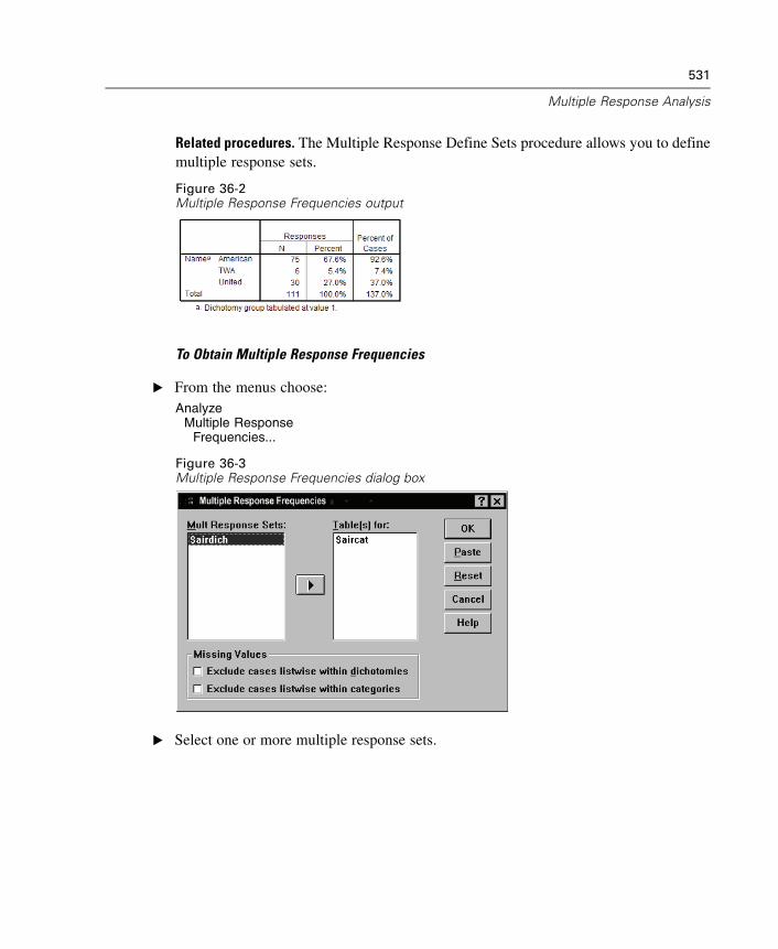
531


Related procedures. The Multiple Response Define Sets procedure allows you to definemultiple response sets.

Figure 36-2Multiple Response Frequencies output

To Obtain Multiple Response Frequencies


Multiple ResponseFrequencies...

Figure 36-3Multiple Response Frequencies dialog box

E Select one or more multiple response sets.

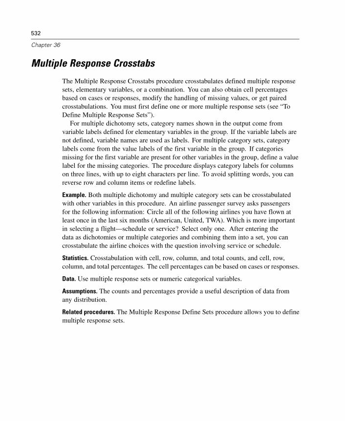
532

Chapter 36

Multiple Response Crosstabs

The Multiple Response Crosstabs procedure crosstabulates defined multiple responsesets, elementary variables, or a combination. You can also obtain cell percentagesbased on cases or responses, modify the handling of missing values, or get pairedcrosstabulations. You must first define one or more multiple response sets (see “ToDefine Multiple Response Sets”).

For multiple dichotomy sets, category names shown in the output come fromvariable labels defined for elementary variables in the group. If the variable labels arenot defined, variable names are used as labels. For multiple category sets, categorylabels come from the value labels of the first variable in the group. If categoriesmissing for the first variable are present for other variables in the group, define a valuelabel for the missing categories. The procedure displays category labels for columnson three lines, with up to eight characters per line. To avoid splitting words, you canreverse row and column items or redefine labels.

Example. Both multiple dichotomy and multiple category sets can be crosstabulatedwith other variables in this procedure. An airline passenger survey asks passengersfor the following information: Circle all of the following airlines you have flown atleast once in the last six months (American, United, TWA). Which is more importantin selecting a flight—schedule or service? Select only one. After entering thedata as dichotomies or multiple categories and combining them into a set, you cancrosstabulate the airline choices with the question involving service or schedule.

Statistics. Crosstabulation with cell, row, column, and total counts, and cell, row,column, and total percentages. The cell percentages can be based on cases or responses.

Data. Use multiple response sets or numeric categorical variables.

Assumptions. The counts and percentages provide a useful description of data fromany distribution.

Related procedures. The Multiple Response Define Sets procedure allows you to definemultiple response sets.

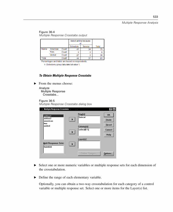
533


Figure 36-4Multiple Response Crosstabs output

To Obtain Multiple Response Crosstabs


Multiple ResponseCrosstabs...

Figure 36-5Multiple Response Crosstabs dialog box

E Select one or more numeric variables or multiple response sets for each dimension ofthe crosstabulation.

E Define the range of each elementary variable.

Optionally, you can obtain a two-way crosstabulation for each category of a controlvariable or multiple response set. Select one or more items for the Layer(s) list.

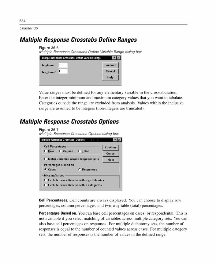
534

Chapter 36

Multiple Response Crosstabs Define RangesFigure 36-6Multiple Response Crosstabs Define Variable Range dialog box

Value ranges must be defined for any elementary variable in the crosstabulation.Enter the integer minimum and maximum category values that you want to tabulate.Categories outside the range are excluded from analysis. Values within the inclusiverange are assumed to be integers (non-integers are truncated).

Multiple Response Crosstabs OptionsFigure 36-7Multiple Response Crosstabs Options dialog box

Cell Percentages. Cell counts are always displayed. You can choose to display rowpercentages, column percentages, and two-way table (total) percentages.

Percentages Based on. You can base cell percentages on cases (or respondents). This isnot available if you select matching of variables across multiple category sets. You canalso base cell percentages on responses. For multiple dichotomy sets, the number ofresponses is equal to the number of counted values across cases. For multiple categorysets, the number of responses is the number of values in the defined range.

535


Missing Values. You can choose one or both of the following:

Exclude cases listwise within dichotomies. Excludes cases with missing valuesfor any variable from the tabulation of the multiple dichotomy set. This appliesonly to multiple response sets defined as dichotomy sets. By default, a caseis considered missing for a multiple dichotomy set if none of its componentvariables contains the counted value. Cases with missing values for some, but notall, variables are included in the tabulations of the group if at least one variablecontains the counted value.

Exclude cases listwise within categories. Excludes cases with missing values forany variable from tabulation of the multiple category set. This applies only tomultiple response sets defined as category sets. By default, a case is consideredmissing for a multiple category set only if none of its components has valid valueswithin the defined range.

By default, when crosstabulating two multiple category sets, the procedure tabulateseach variable in the first group with each variable in the second group and sums thecounts for each cell; therefore, some responses can appear more than once in a table.You can choose the following option:

Match variables across response sets. Pairs the first variable in the first group with thefirst variable in the second group, and so on. If you select this option, the procedurebases cell percentages on responses rather than respondents. Pairing is not availablefor multiple dichotomy sets or elementary variables.

MULT RESPONSE Command Additional Features


Obtain crosstabulation tables with up to five dimensions (with the BYsubcommand).

Change output formatting options, including suppression of value labels (with theFORMAT subcommand).


Chapter

37Reporting Results

Case listings and descriptive statistics are basic tools for studying and presentingdata. You can obtain case listings with the Data Editor or the Summarize procedure,frequency counts and descriptive statistics with the Frequencies procedure, andsubpopulation statistics with the Means procedure. Each of these uses a formatdesigned to make information clear. If you want to display the information in adifferent format, Report Summaries in Rows and Report Summaries in Columns giveyou the control you need over data presentation.

Report Summaries in Rows

Report Summaries in Rows produces reports in which different summary statistics arelaid out in rows. Case listings are also available, with or without summary statistics.

Example. A company with a chain of retail stores keeps records of employeeinformation, including salary, job tenure, and the store and division in which eachemployee works. You could generate a report that provides individual employeeinformation (listing) broken down by store and division (break variables), withsummary statistics (for example, mean salary) for each store, division, and divisionwithin each store.

Data Columns. Lists the report variables for which you want case listings or summarystatistics and controls the display format of data columns.

Break Columns. Lists optional break variables that divide the report into groups andcontrols the summary statistics and display formats of break columns. For multiplebreak variables, there will be a separate group for each category of each break variablewithin categories of the preceding break variable in the list. Break variables should bediscrete categorical variables that divide cases into a limited number of meaningfulcategories. Individual values of each break variable appear, sorted, in a separatecolumn to the left of all data columns.

537

538

Chapter 37

Report. Controls overall report characteristics, including overall summary statistics,display of missing values, page numbering, and titles.

Display cases. Displays the actual values (or value labels) of the data-column variablesfor every case. This produces a listing report, which can be much longer than asummary report.

Preview. Displays only the first page of the report. This option is useful for previewingthe format of your report without processing the whole report.

Data are already sorted. For reports with break variables, the data file must be sorted bybreak variable values before generating the report. If your data file is already sorted byvalues of the break variables, you can save processing time by selecting this option.This option is particularly useful after running a preview report.

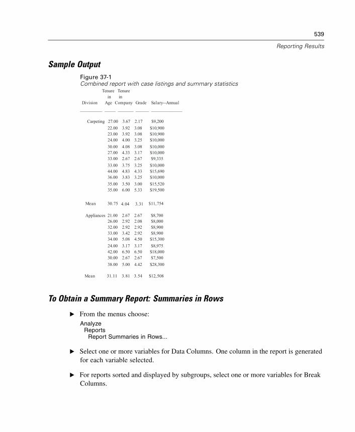
539

Reporting Results

Sample OutputFigure 37-1Combined report with case listings and summary statistics

To Obtain a Summary Report: Summaries in Rows


ReportsReport Summaries in Rows...

E Select one or more variables for Data Columns. One column in the report is generatedfor each variable selected.

E For reports sorted and displayed by subgroups, select one or more variables for BreakColumns.

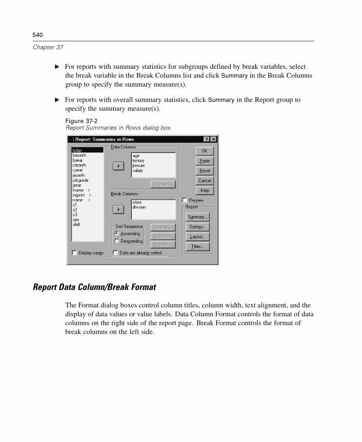
540

Chapter 37

E For reports with summary statistics for subgroups defined by break variables, selectthe break variable in the Break Columns list and click Summary in the Break Columnsgroup to specify the summary measure(s).

E For reports with overall summary statistics, click Summary in the Report group tospecify the summary measure(s).

Figure 37-2Report Summaries in Rows dialog box

Report Data Column/Break Format

The Format dialog boxes control column titles, column width, text alignment, and thedisplay of data values or value labels. Data Column Format controls the format of datacolumns on the right side of the report page. Break Format controls the format ofbreak columns on the left side.

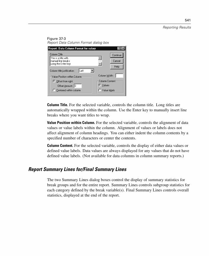
541

Reporting Results

Figure 37-3Report Data Column Format dialog box

Column Title. For the selected variable, controls the column title. Long titles areautomatically wrapped within the column. Use the Enter key to manually insert linebreaks where you want titles to wrap.

Value Position within Column. For the selected variable, controls the alignment of datavalues or value labels within the column. Alignment of values or labels does notaffect alignment of column headings. You can either indent the column contents by aspecified number of characters or center the contents.

Column Content. For the selected variable, controls the display of either data values ordefined value labels. Data values are always displayed for any values that do not havedefined value labels. (Not available for data columns in column summary reports.)

Report Summary Lines for/Final Summary Lines

The two Summary Lines dialog boxes control the display of summary statistics forbreak groups and for the entire report. Summary Lines controls subgroup statistics foreach category defined by the break variable(s). Final Summary Lines controls overallstatistics, displayed at the end of the report.

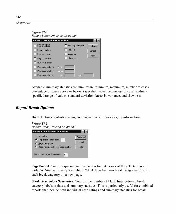
542

Chapter 37

Figure 37-4Report Summary Lines dialog box

Available summary statistics are sum, mean, minimum, maximum, number of cases,percentage of cases above or below a specified value, percentage of cases within aspecified range of values, standard deviation, kurtosis, variance, and skewness.

Report Break Options

Break Options controls spacing and pagination of break category information.

Figure 37-5Report Break Options dialog box

Page Control. Controls spacing and pagination for categories of the selected breakvariable. You can specify a number of blank lines between break categories or starteach break category on a new page.

Blank Lines before Summaries. Controls the number of blank lines between breakcategory labels or data and summary statistics. This is particularly useful for combinedreports that include both individual case listings and summary statistics for break

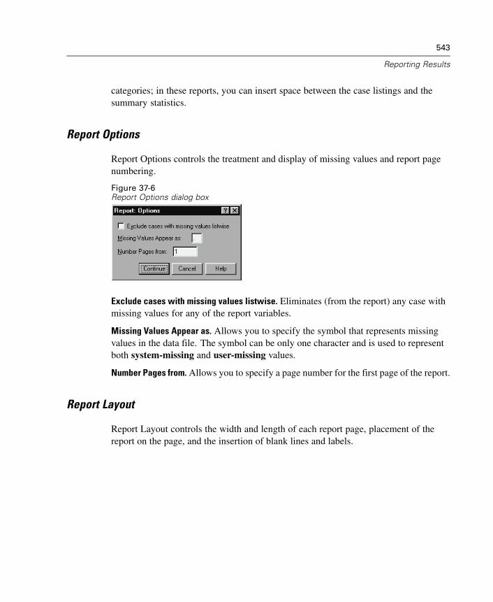
543

Reporting Results

categories; in these reports, you can insert space between the case listings and thesummary statistics.

Report Options

Report Options controls the treatment and display of missing values and report pagenumbering.

Figure 37-6Report Options dialog box

Exclude cases with missing values listwise. Eliminates (from the report) any case withmissing values for any of the report variables.

Missing Values Appear as. Allows you to specify the symbol that represents missingvalues in the data file. The symbol can be only one character and is used to representboth system-missing and user-missing values.

Number Pages from. Allows you to specify a page number for the first page of the report.

Report Layout

Report Layout controls the width and length of each report page, placement of thereport on the page, and the insertion of blank lines and labels.

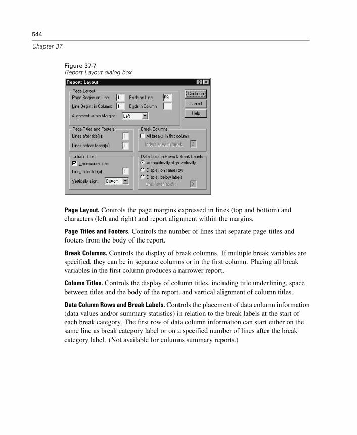
544

Chapter 37

Figure 37-7Report Layout dialog box

Page Layout. Controls the page margins expressed in lines (top and bottom) andcharacters (left and right) and report alignment within the margins.

Page Titles and Footers. Controls the number of lines that separate page titles andfooters from the body of the report.

Break Columns. Controls the display of break columns. If multiple break variables arespecified, they can be in separate columns or in the first column. Placing all breakvariables in the first column produces a narrower report.

Column Titles. Controls the display of column titles, including title underlining, spacebetween titles and the body of the report, and vertical alignment of column titles.

Data Column Rows and Break Labels. Controls the placement of data column information(data values and/or summary statistics) in relation to the break labels at the start ofeach break category. The first row of data column information can start either on thesame line as break category label or on a specified number of lines after the breakcategory label. (Not available for columns summary reports.)

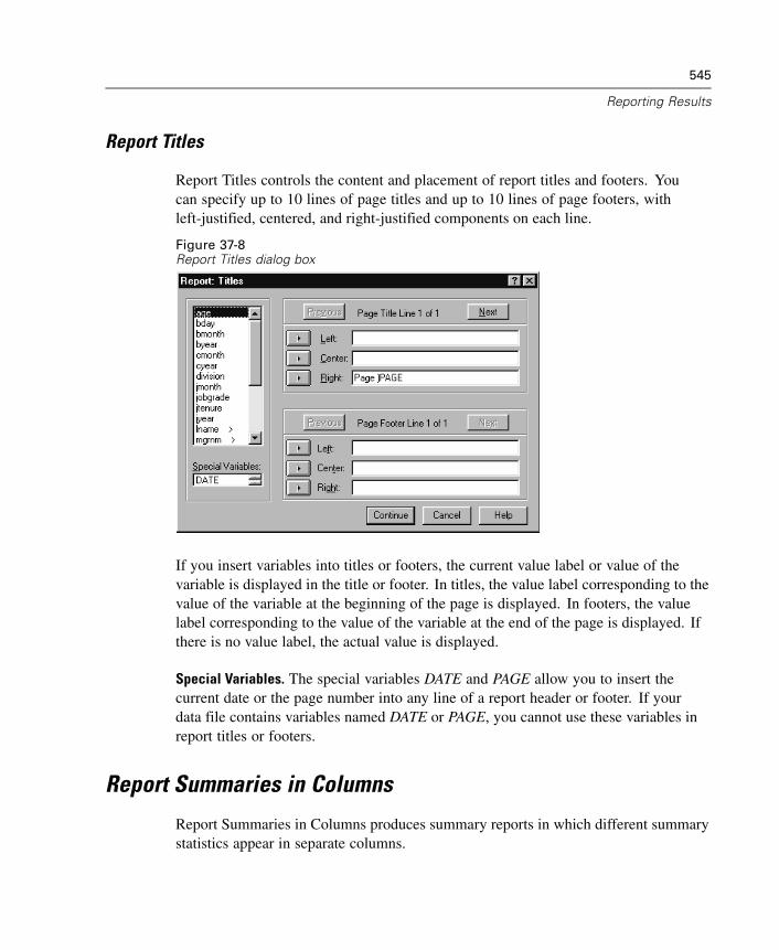
545

Reporting Results

Report Titles

Report Titles controls the content and placement of report titles and footers. Youcan specify up to 10 lines of page titles and up to 10 lines of page footers, withleft-justified, centered, and right-justified components on each line.

Figure 37-8Report Titles dialog box

If you insert variables into titles or footers, the current value label or value of thevariable is displayed in the title or footer. In titles, the value label corresponding to thevalue of the variable at the beginning of the page is displayed. In footers, the valuelabel corresponding to the value of the variable at the end of the page is displayed. Ifthere is no value label, the actual value is displayed.

Special Variables. The special variables DATE and PAGE allow you to insert thecurrent date or the page number into any line of a report header or footer. If yourdata file contains variables named DATE or PAGE, you cannot use these variables inreport titles or footers.

Report Summaries in Columns

Report Summaries in Columns produces summary reports in which different summarystatistics appear in separate columns.

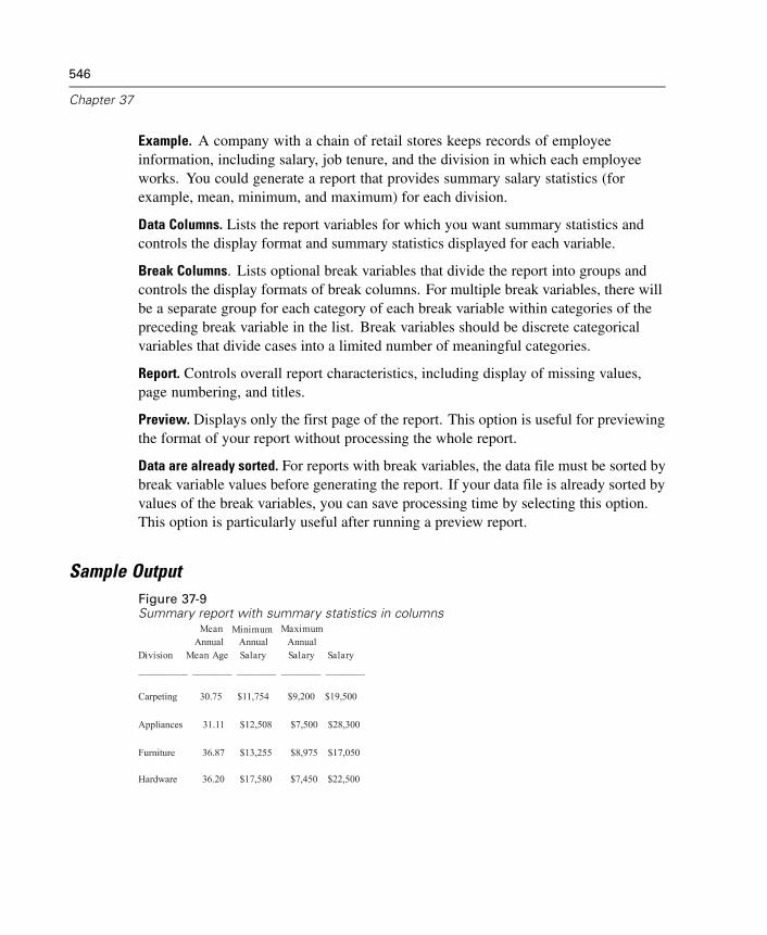
546

Chapter 37

Example. A company with a chain of retail stores keeps records of employeeinformation, including salary, job tenure, and the division in which each employeeworks. You could generate a report that provides summary salary statistics (forexample, mean, minimum, and maximum) for each division.

Data Columns. Lists the report variables for which you want summary statistics andcontrols the display format and summary statistics displayed for each variable.

Break Columns. Lists optional break variables that divide the report into groups andcontrols the display formats of break columns. For multiple break variables, there willbe a separate group for each category of each break variable within categories of thepreceding break variable in the list. Break variables should be discrete categoricalvariables that divide cases into a limited number of meaningful categories.

Report. Controls overall report characteristics, including display of missing values,page numbering, and titles.

Preview. Displays only the first page of the report. This option is useful for previewingthe format of your report without processing the whole report.

Data are already sorted. For reports with break variables, the data file must be sorted bybreak variable values before generating the report. If your data file is already sorted byvalues of the break variables, you can save processing time by selecting this option.This option is particularly useful after running a preview report.

Sample OutputFigure 37-9Summary report with summary statistics in columns

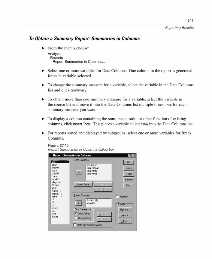
547

Reporting Results

To Obtain a Summary Report: Summaries in Columns


ReportsReport Summaries in Columns...

E Select one or more variables for Data Columns. One column in the report is generatedfor each variable selected.

E To change the summary measure for a variable, select the variable in the Data Columnslist and click Summary.

E To obtain more than one summary measure for a variable, select the variable inthe source list and move it into the Data Columns list multiple times, one for eachsummary measure you want.

E To display a column containing the sum, mean, ratio, or other function of existingcolumns, click Insert Total. This places a variable called total into the Data Columns list.

E For reports sorted and displayed by subgroups, select one or more variables for BreakColumns.

Figure 37-10Report Summaries in Columns dialog box

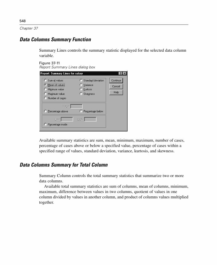
548

Chapter 37

Data Columns Summary Function

Summary Lines controls the summary statistic displayed for the selected data columnvariable.

Figure 37-11Report Summary Lines dialog box

Available summary statistics are sum, mean, minimum, maximum, number of cases,percentage of cases above or below a specified value, percentage of cases within aspecified range of values, standard deviation, variance, kurtosis, and skewness.

Data Columns Summary for Total Column

Summary Column controls the total summary statistics that summarize two or moredata columns.

Available total summary statistics are sum of columns, mean of columns, minimum,maximum, difference between values in two columns, quotient of values in onecolumn divided by values in another column, and product of columns values multipliedtogether.

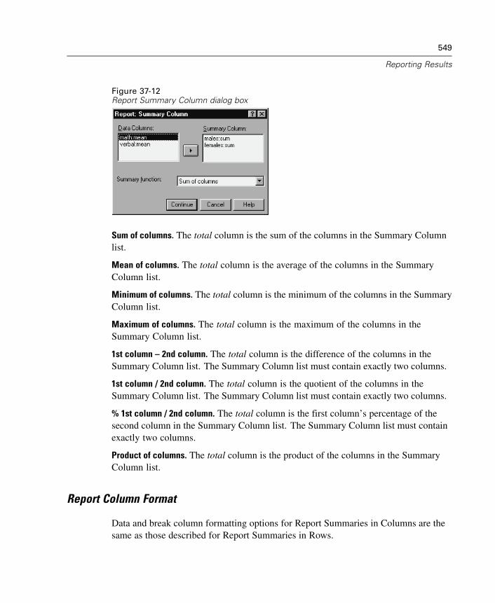
549

Reporting Results

Figure 37-12Report Summary Column dialog box

Sum of columns. The total column is the sum of the columns in the Summary Columnlist.

Mean of columns. The total column is the average of the columns in the SummaryColumn list.

Minimum of columns. The total column is the minimum of the columns in the SummaryColumn list.

Maximum of columns. The total column is the maximum of the columns in theSummary Column list.

1st column – 2nd column. The total column is the difference of the columns in theSummary Column list. The Summary Column list must contain exactly two columns.

1st column / 2nd column. The total column is the quotient of the columns in theSummary Column list. The Summary Column list must contain exactly two columns.

% 1st column / 2nd column. The total column is the first column’s percentage of thesecond column in the Summary Column list. The Summary Column list must containexactly two columns.

Product of columns. The total column is the product of the columns in the SummaryColumn list.

Report Column Format

Data and break column formatting options for Report Summaries in Columns are thesame as those described for Report Summaries in Rows.

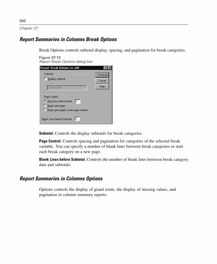
550

Chapter 37

Report Summaries in Columns Break Options

Break Options controls subtotal display, spacing, and pagination for break categories.

Figure 37-13Report Break Options dialog box

Subtotal. Controls the display subtotals for break categories.

Page Control. Controls spacing and pagination for categories of the selected breakvariable. You can specify a number of blank lines between break categories or starteach break category on a new page.

Blank Lines before Subtotal. Controls the number of blank lines between break categorydata and subtotals.

Report Summaries in Columns Options

Options controls the display of grand totals, the display of missing values, andpagination in column summary reports.

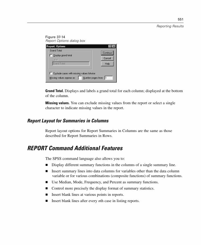
551

Reporting Results

Figure 37-14Report Options dialog box

Grand Total. Displays and labels a grand total for each column; displayed at the bottomof the column.

Missing values. You can exclude missing values from the report or select a singlecharacter to indicate missing values in the report.

Report Layout for Summaries in Columns

Report layout options for Report Summaries in Columns are the same as thosedescribed for Report Summaries in Rows.

REPORT Command Additional Features


Display different summary functions in the columns of a single summary line.

Insert summary lines into data columns for variables other than the data columnvariable or for various combinations (composite functions) of summary functions.

Use Median, Mode, Frequency, and Percent as summary functions.

Control more precisely the display format of summary statistics.

Insert blank lines at various points in reports.

Insert blank lines after every nth case in listing reports.

552

Chapter 37

Because of the complexity of the REPORT syntax, you may find it useful, whenbuilding a new report with syntax, to approximate the report generated from thedialog boxes, copy and paste the corresponding syntax, and refine that syntax to yieldthe exact report that you want.


Chapter

38Reliability Analysis

Reliability analysis allows you to study the properties of measurement scales andthe items that compose the scales. The Reliability Analysis procedure calculates anumber of commonly used measures of scale reliability and also provides informationabout the relationships between individual items in the scale. Intraclass correlationcoefficients can be used to compute inter-rater reliability estimates.

Example. Does my questionnaire measure customer satisfaction in a useful way?Using reliability analysis, you can determine the extent to which the items in yourquestionnaire are related to each other, you can get an overall index of the repeatabilityor internal consistency of the scale as a whole, and you can identify problem itemsthat should be excluded from the scale.

Statistics. Descriptives for each variable and for the scale, summary statistics acrossitems, inter-item correlations and covariances, reliability estimates, ANOVA table,intraclass correlation coefficients, Hotelling’s T2, and Tukey’s test of additivity.

Models. The following models of reliability are available:

Alpha (Cronbach). This model is a model of internal consistency, based on theaverage inter-item correlation.

Split-half. This model splits the scale into two parts and examines the correlationbetween the parts.

Guttman. This model computes Guttman’s lower bounds for true reliability.

Parallel. This model assumes that all items have equal variances and equal errorvariances across replications.

Strict parallel. This model makes the assumptions of the Parallel model and alsoassumes equal means across items.

Data. Data can be dichotomous, ordinal, or interval, but the data should be codednumerically.

553

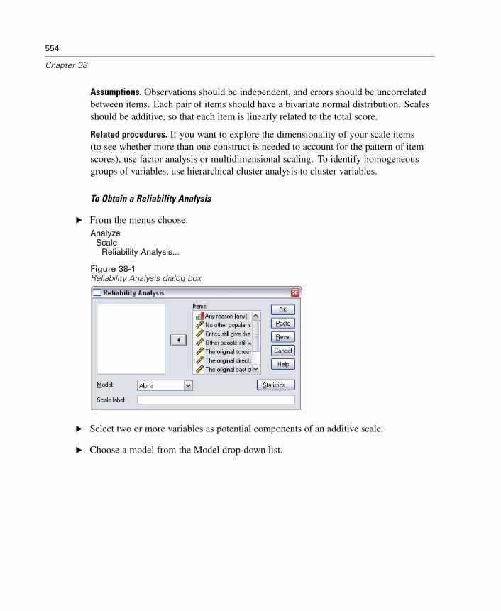
554

Chapter 38

Assumptions. Observations should be independent, and errors should be uncorrelatedbetween items. Each pair of items should have a bivariate normal distribution. Scalesshould be additive, so that each item is linearly related to the total score.

Related procedures. If you want to explore the dimensionality of your scale items(to see whether more than one construct is needed to account for the pattern of itemscores), use factor analysis or multidimensional scaling. To identify homogeneousgroups of variables, use hierarchical cluster analysis to cluster variables.

To Obtain a Reliability Analysis


ScaleReliability Analysis...

Figure 38-1Reliability Analysis dialog box

E Select two or more variables as potential components of an additive scale.

E Choose a model from the Model drop-down list.

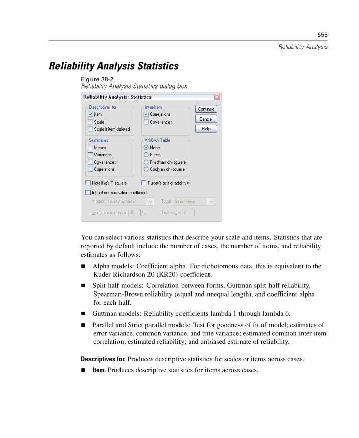
555

Reliability Analysis

Reliability Analysis StatisticsFigure 38-2Reliability Analysis Statistics dialog box

You can select various statistics that describe your scale and items. Statistics that arereported by default include the number of cases, the number of items, and reliabilityestimates as follows:

Alpha models: Coefficient alpha. For dichotomous data, this is equivalent to theKuder-Richardson 20 (KR20) coefficient.

Split-half models: Correlation between forms, Guttman split-half reliability,Spearman-Brown reliability (equal and unequal length), and coefficient alphafor each half.

Guttman models: Reliability coefficients lambda 1 through lambda 6.

Parallel and Strict parallel models: Test for goodness of fit of model; estimates oferror variance, common variance, and true variance; estimated common inter-itemcorrelation; estimated reliability; and unbiased estimate of reliability.

Descriptives for. Produces descriptive statistics for scales or items across cases.

Item. Produces descriptive statistics for items across cases.

556

Chapter 38

Scale. Produces descriptive statistics for scales.

Scale if item deleted. Displays summary statistics comparing each item to the scalethat is composed of the other items. Statistics include scale mean and varianceif the item were to be deleted from the scale, correlation between the item andthe scale that is composed of other items, and Cronbach’s alpha if the item wereto be deleted from the scale.

Summaries. Provides descriptive statistics of item distributions across all items inthe scale.

Means. Summary statistics for item means. The smallest, largest, and averageitem means, the range and variance of item means, and the ratio of the largest tothe smallest item means are displayed.

Variances. Summary statistics for item variances. The smallest, largest, andaverage item variances, the range and variance of item variances, and the ratio ofthe largest to the smallest item variances are displayed.

Covariances. Summary statistics for inter-item covariances. The smallest,largest, and average inter-item covariances, the range and variance of inter-itemcovariances, and the ratio of the largest to the smallest inter-item covariancesare displayed.

Correlations. Summary statistics for inter-item correlations. The smallest,largest, and average inter-item correlations, the range and variance of inter-itemcorrelations, and the ratio of the largest to the smallest inter-item correlationsare displayed.

Inter-Item. Produces matrices of correlations or covariances between items.

ANOVA Table. Produces tests of equal means.

F test. Displays a repeated measures analysis-of-variance table.

Friedman chi-square. Displays Friedman's chi-square and Kendall's coefficient ofconcordance. This option is appropriate for data that are in the form of ranks. Thechi-square test replaces the usual F test in the ANOVA table.

Cochran chi-square. Displays Cochran's Q. This option is appropriate for data thatare dichotomous. The Q statistic replaces the usual F statistic in the ANOVA table.

Hotelling’s T-square. Produces a multivariate test of the null hypothesis that all items onthe scale have the same mean.

557

Reliability Analysis

Tukey’s test of additivity. Produces a test of the assumption that there is no multiplicativeinteraction among the items.

Intraclass correlation coefficient. Produces measures of consistency or agreement ofvalues within cases.

Model. Select the model for calculating the intraclass correlation coefficient.Available models are Two-Way Mixed, Two-Way Random, and One-Way Random.Select Two-Way Mixed when people effects are random and the item effects arefixed, select Two-Way Random when people effects and the item effects are random.Select One-Way Random when people effects are random.

Type. Select the type of index. Available types are Consistency and AbsoluteAgreement.

Confidence interval. Specify the level for the confidence interval. The default is95%.

Test value. Specify the hypothesized value of the coefficient for the hypothesis test.This value is the value to which the observed value is compared. The defaultvalue is 0.

RELIABILITY Command Additional Features


Read and analyze a correlation matrix.

Write a correlation matrix for later analysis.

Specify splits other than equal halves for the split-half method.


Chapter

39Multidimensional Scaling

Multidimensional scaling attempts to find the structure in a set of distance measuresbetween objects or cases. This task is accomplished by assigning observations tospecific locations in a conceptual space (usually two- or three-dimensional) such thatthe distances between points in the space match the given dissimilarities as closely aspossible. In many cases, the dimensions of this conceptual space can be interpretedand used to further understand your data.

If you have objectively measured variables, you can use multidimensional scalingas a data reduction technique (the Multidimensional Scaling procedure will computedistances from multivariate data for you, if necessary). Multidimensional scaling canalso be applied to subjective ratings of dissimilarity between objects or concepts.Additionally, the Multidimensional Scaling procedure can handle dissimilarity datafrom multiple sources, as you might have with multiple raters or questionnairerespondents.

Example. How do people perceive relationships between different cars? If you havedata from respondents indicating similarity ratings between different makes andmodels of cars, multidimensional scaling can be used to identify dimensions thatdescribe consumers’ perceptions. You might find, for example, that the price andsize of a vehicle define a two-dimensional space, which accounts for the similaritiesthat are reported by your respondents.

Statistics. For each model: data matrix, optimally scaled data matrix, S-stress(Young’s), stress (Kruskal’s), RSQ, stimulus coordinates, average stress and RSQfor each stimulus (RMDS models). For individual difference (INDSCAL) models:subject weights and weirdness index for each subject. For each matrix in replicatedmultidimensional scaling models: stress and RSQ for each stimulus. Plots: stimuluscoordinates (two- or three-dimensional), scatterplot of disparities versus distances.

559

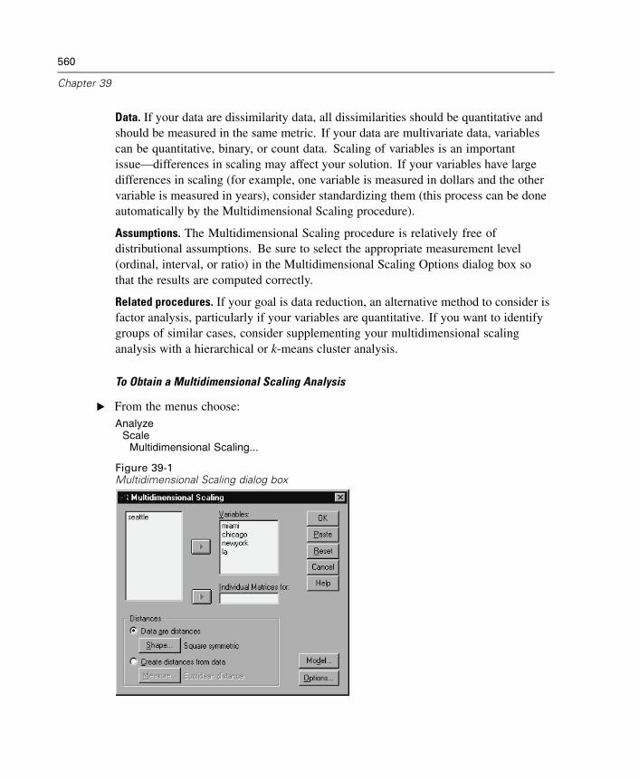
560

Chapter 39

Data. If your data are dissimilarity data, all dissimilarities should be quantitative andshould be measured in the same metric. If your data are multivariate data, variablescan be quantitative, binary, or count data. Scaling of variables is an importantissue—differences in scaling may affect your solution. If your variables have largedifferences in scaling (for example, one variable is measured in dollars and the othervariable is measured in years), consider standardizing them (this process can be doneautomatically by the Multidimensional Scaling procedure).

Assumptions. The Multidimensional Scaling procedure is relatively free ofdistributional assumptions. Be sure to select the appropriate measurement level(ordinal, interval, or ratio) in the Multidimensional Scaling Options dialog box sothat the results are computed correctly.

Related procedures. If your goal is data reduction, an alternative method to consider isfactor analysis, particularly if your variables are quantitative. If you want to identifygroups of similar cases, consider supplementing your multidimensional scalinganalysis with a hierarchical or k-means cluster analysis.

To Obtain a Multidimensional Scaling Analysis


ScaleMultidimensional Scaling...

Figure 39-1Multidimensional Scaling dialog box

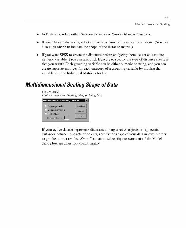
561

Multidimensional Scaling

E In Distances, select either Data are distances or Create distances from data.

E If your data are distances, select at least four numeric variables for analysis. (You canalso click Shape to indicate the shape of the distance matrix.)

E If you want SPSS to create the distances before analyzing them, select at least onenumeric variable. (You can also click Measure to specify the type of distance measurethat you want.) Each grouping variable can be either numeric or string, and you cancreate separate matrices for each category of a grouping variable by moving thatvariable into the Individual Matrices for list.

Multidimensional Scaling Shape of DataFigure 39-2Multidimensional Scaling Shape dialog box

If your active dataset represents distances among a set of objects or representsdistances between two sets of objects, specify the shape of your data matrix in orderto get the correct results. Note: You cannot select Square symmetric if the Modeldialog box specifies row conditionality.

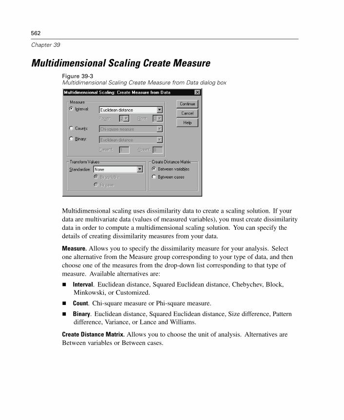
562

Chapter 39

Multidimensional Scaling Create MeasureFigure 39-3Multidimensional Scaling Create Measure from Data dialog box

Multidimensional scaling uses dissimilarity data to create a scaling solution. If yourdata are multivariate data (values of measured variables), you must create dissimilaritydata in order to compute a multidimensional scaling solution. You can specify thedetails of creating dissimilarity measures from your data.

Measure. Allows you to specify the dissimilarity measure for your analysis. Selectone alternative from the Measure group corresponding to your type of data, and thenchoose one of the measures from the drop-down list corresponding to that type ofmeasure. Available alternatives are:

Interval. Euclidean distance, Squared Euclidean distance, Chebychev, Block,Minkowski, or Customized.

Count. Chi-square measure or Phi-square measure.

Binary. Euclidean distance, Squared Euclidean distance, Size difference, Patterndifference, Variance, or Lance and Williams.

Create Distance Matrix. Allows you to choose the unit of analysis. Alternatives areBetween variables or Between cases.

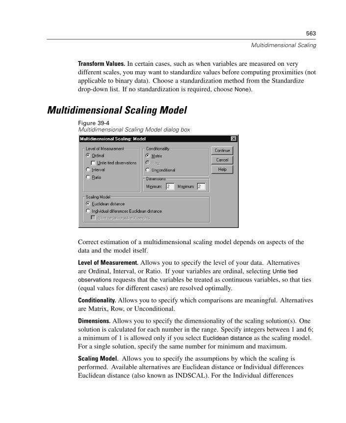
563


Transform Values. In certain cases, such as when variables are measured on verydifferent scales, you may want to standardize values before computing proximities (notapplicable to binary data). Choose a standardization method from the Standardizedrop-down list. If no standardization is required, choose None).

Multidimensional Scaling ModelFigure 39-4Multidimensional Scaling Model dialog box

Correct estimation of a multidimensional scaling model depends on aspects of thedata and the model itself.

Level of Measurement. Allows you to specify the level of your data. Alternativesare Ordinal, Interval, or Ratio. If your variables are ordinal, selecting Untie tied

observations requests that the variables be treated as continuous variables, so that ties(equal values for different cases) are resolved optimally.

Conditionality. Allows you to specify which comparisons are meaningful. Alternativesare Matrix, Row, or Unconditional.

Dimensions. Allows you to specify the dimensionality of the scaling solution(s). Onesolution is calculated for each number in the range. Specify integers between 1 and 6;a minimum of 1 is allowed only if you select Euclidean distance as the scaling model.For a single solution, specify the same number for minimum and maximum.

Scaling Model. Allows you to specify the assumptions by which the scaling isperformed. Available alternatives are Euclidean distance or Individual differencesEuclidean distance (also known as INDSCAL). For the Individual differences

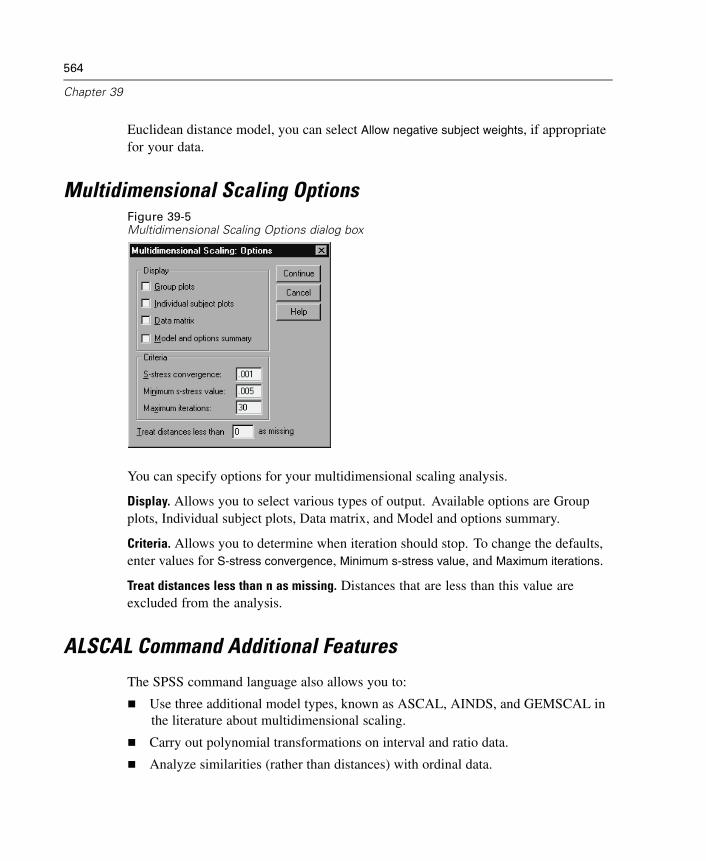
564

Chapter 39

Euclidean distance model, you can select Allow negative subject weights, if appropriatefor your data.

Multidimensional Scaling OptionsFigure 39-5Multidimensional Scaling Options dialog box

You can specify options for your multidimensional scaling analysis.

Display. Allows you to select various types of output. Available options are Groupplots, Individual subject plots, Data matrix, and Model and options summary.

Criteria. Allows you to determine when iteration should stop. To change the defaults,enter values for S-stress convergence, Minimum s-stress value, and Maximum iterations.

Treat distances less than n as missing. Distances that are less than this value areexcluded from the analysis.

ALSCAL Command Additional Features


Use three additional model types, known as ASCAL, AINDS, and GEMSCAL inthe literature about multidimensional scaling.

Carry out polynomial transformations on interval and ratio data.

Analyze similarities (rather than distances) with ordinal data.

565


Analyze nominal data.

Save various coordinate and weight matrices into files and read them back in foranalysis.

Constrain multidimensional unfolding.


Chapter

40Ratio Statistics

The Ratio Statistics procedure provides a comprehensive list of summary statistics fordescribing the ratio between two scale variables.

You can sort the output by values of a grouping variable in ascending or descendingorder. The ratio statistics report can be suppressed in the output, and the results can besaved to an external file.

Example. Is there good uniformity in the ratio between the appraisal price and saleprice of homes in each of five counties? From the output, you might learn that thedistribution of ratios varies considerably from county to county.

Statistics. Median, mean, weighted mean, confidence intervals, coefficient ofdispersion (COD), median-centered coefficient of variation, mean-centered coefficientof variation, price-related differential (PRD), standard deviation, average absolutedeviation (AAD), range, minimum and maximum values, and the concentration indexcomputed for a user-specified range or percentage within the median ratio.

Data. Use numeric codes or short strings to code grouping variables (nominal orordinal level measurements).

Assumptions. The variables that define the numerator and denominator of the ratioshould be scale variables that take positive values.

To Obtain Ratio Statistics


Descriptive StatisticsRatio...

567

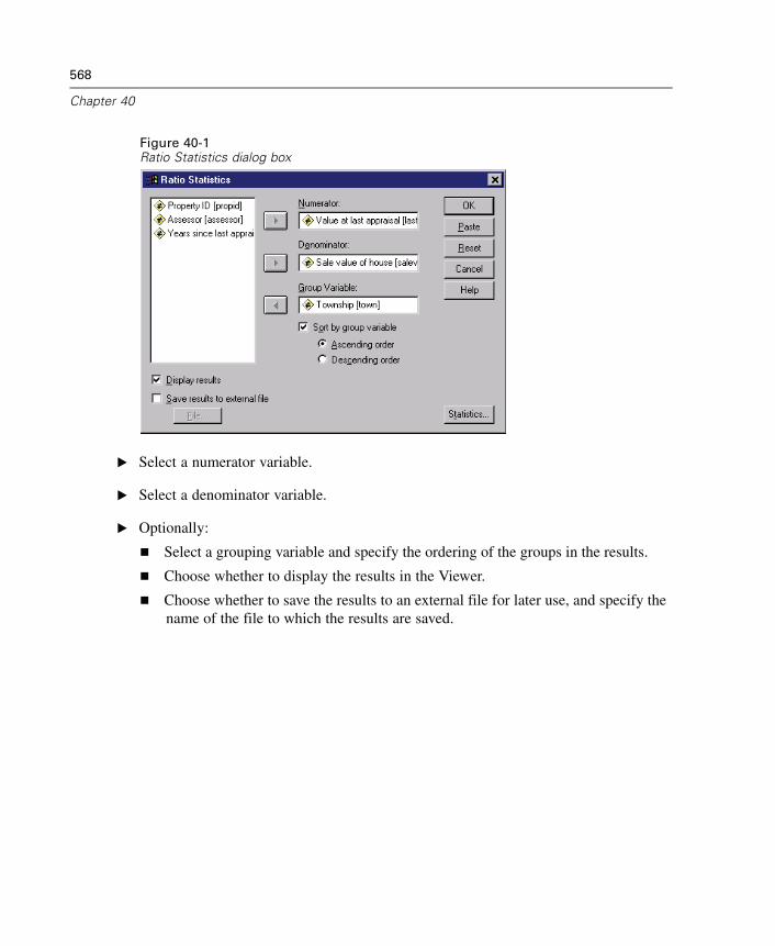
568

Chapter 40

Figure 40-1Ratio Statistics dialog box

E Select a numerator variable.

E Select a denominator variable.

E Optionally:

Select a grouping variable and specify the ordering of the groups in the results.

Choose whether to display the results in the Viewer.

Choose whether to save the results to an external file for later use, and specify thename of the file to which the results are saved.

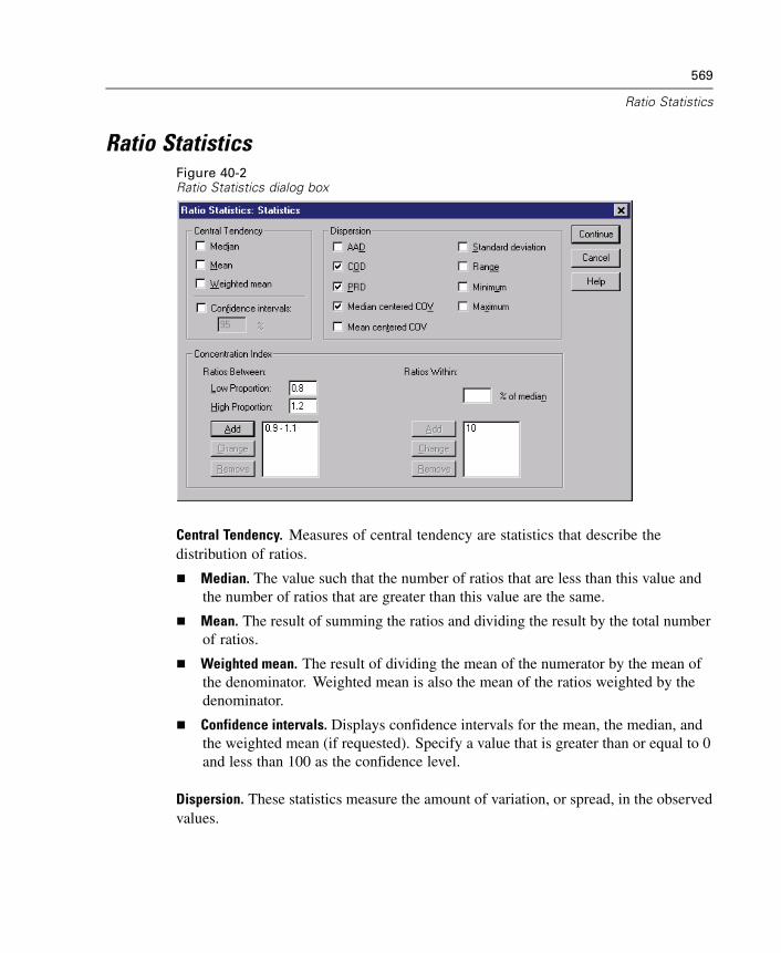
569

Ratio Statistics

Ratio StatisticsFigure 40-2Ratio Statistics dialog box

Central Tendency. Measures of central tendency are statistics that describe thedistribution of ratios.

Median. The value such that the number of ratios that are less than this value andthe number of ratios that are greater than this value are the same.

Mean. The result of summing the ratios and dividing the result by the total numberof ratios.

Weighted mean. The result of dividing the mean of the numerator by the mean ofthe denominator. Weighted mean is also the mean of the ratios weighted by thedenominator.

Confidence intervals. Displays confidence intervals for the mean, the median, andthe weighted mean (if requested). Specify a value that is greater than or equal to 0and less than 100 as the confidence level.

Dispersion. These statistics measure the amount of variation, or spread, in the observedvalues.

570

Chapter 40

AAD. The average absolute deviation is the result of summing the absolutedeviations of the ratios about the median and dividing the result by the totalnumber of ratios.

COD. The coefficient of dispersion is the result of expressing the average absolutedeviation as a percentage of the median.

PRD. The price-related differential, also known as the index of regressivity, is theresult of dividing the mean by the weighted mean.

Median centered COV. The median-centered coefficient of variation is the result ofexpressing the root mean squares of deviation from the median as a percentageof the median.

Mean centered COV. The mean-centered coefficient of variation is the result ofexpressing the standard deviation as a percentage of the mean.

Standard deviation. The standard deviation is the result of summing the squareddeviations of the ratios about the mean, dividing the result by the total number ofratios minus one, and taking the positive square root.

Range. The range is the result of subtracting the minimum ratio from the maximumratio.

Minimum. The minimum is the smallest ratio.

Maximum. The maximum is the largest ratio.

Concentration Index. The coefficient of concentration measures the percentage of ratiosthat fall within an interval. It can be computed in two different ways:

Ratios Between. Here the interval is defined explicitly by specifying the lowand high values of the interval. Enter values for the low proportion and highproportion, and click Add to obtain an interval.

Ratios Within. Here the interval is defined implicitly by specifying the percentageof the median. Enter a value between 0 and 100, and click Add. The lower end ofthe interval is equal to (1 – 0.01 × value) × median, and the upper end is equal to(1 + 0.01 × value) × median.

Chapter

41Overview of the Chart Facility

High-resolution charts and plots are created by the procedures on the Graphs menu andby many of the procedures on the Analyze menu. This chapter provides an overviewof the chart facility.

Creating and Modifying a Chart

Before you can create a chart, you need to have your data in the Data Editor. You canenter the data directly into the Data Editor, open a previously saved data file, or reada spreadsheet, tab-delimited data file, or database file. The Tutorial selection on theHelp menu has online examples of creating and modifying a chart, and the online Helpsystem provides information about creating and modifying all chart types.

Creating the Chart

E After you get your data into the Data Editor, select Chart Builder from the Graphs menu.This opens the Chart Builder dialog box.

571

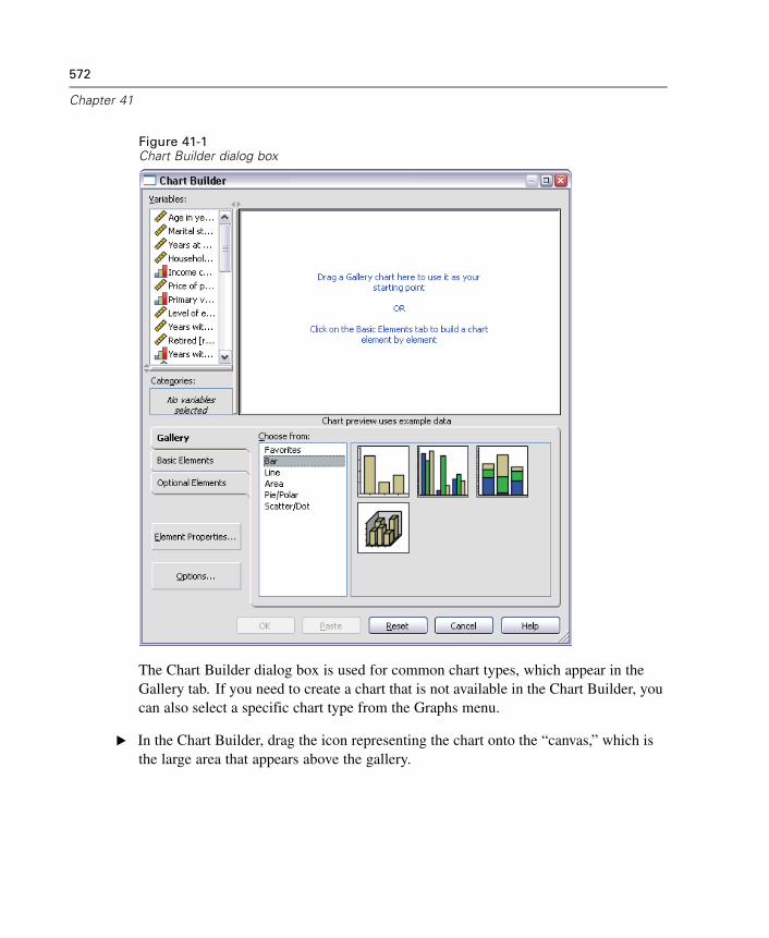
572

Chapter 41

Figure 41-1Chart Builder dialog box

The Chart Builder dialog box is used for common chart types, which appear in theGallery tab. If you need to create a chart that is not available in the Chart Builder, youcan also select a specific chart type from the Graphs menu.

E In the Chart Builder, drag the icon representing the chart onto the “canvas,” which isthe large area that appears above the gallery.

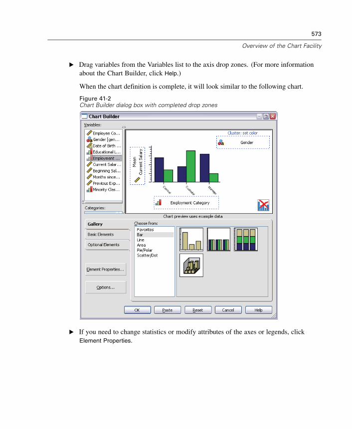
573

Overview of the Chart Facility

E Drag variables from the Variables list to the axis drop zones. (For more informationabout the Chart Builder, click Help.)

When the chart definition is complete, it will look similar to the following chart.

Figure 41-2Chart Builder dialog box with completed drop zones

E If you need to change statistics or modify attributes of the axes or legends, clickElement Properties.

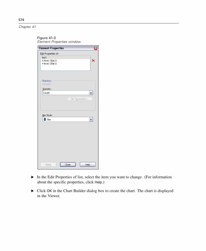
574

Chapter 41

Figure 41-3Element Properties window

E In the Edit Properties of list, select the item you want to change. (For informationabout the specific properties, click Help.)

E Click OK in the Chart Builder dialog box to create the chart. The chart is displayedin the Viewer.

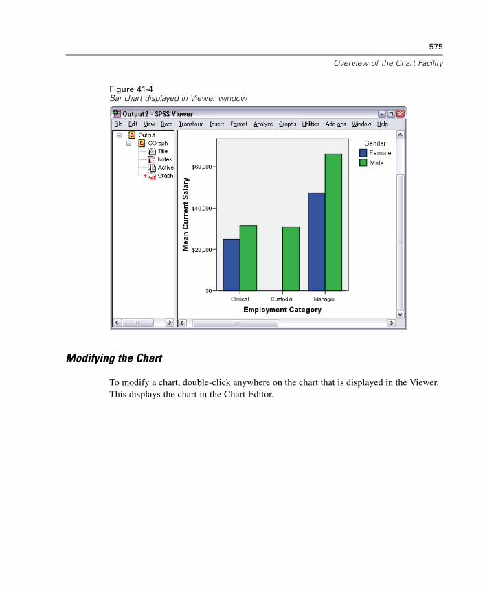
575


Figure 41-4Bar chart displayed in Viewer window

Modifying the Chart

To modify a chart, double-click anywhere on the chart that is displayed in the Viewer.This displays the chart in the Chart Editor.

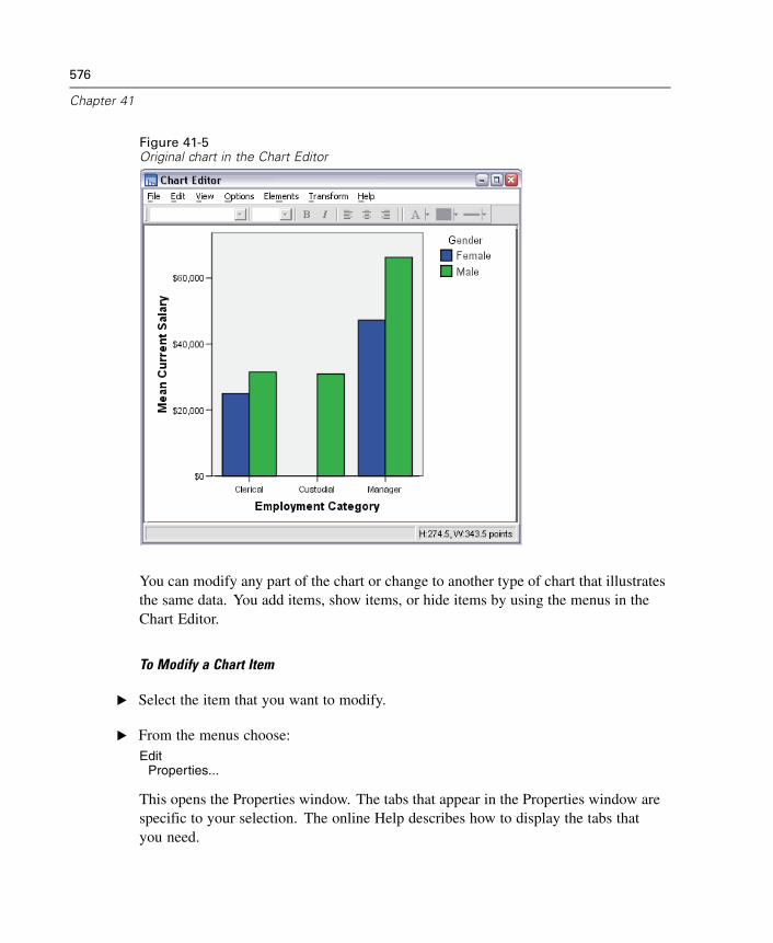
576

Chapter 41

Figure 41-5Original chart in the Chart Editor

You can modify any part of the chart or change to another type of chart that illustratesthe same data. You add items, show items, or hide items by using the menus in theChart Editor.

To Modify a Chart Item

E Select the item that you want to modify.


Properties...

This opens the Properties window. The tabs that appear in the Properties window arespecific to your selection. The online Help describes how to display the tabs thatyou need.

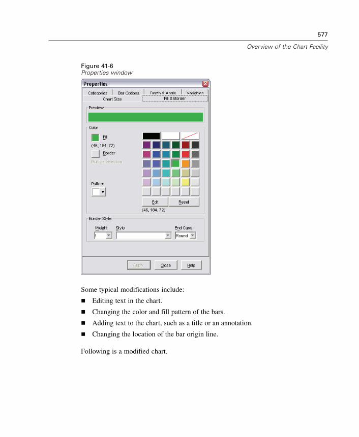
577


Figure 41-6Properties window

Some typical modifications include:

Editing text in the chart.

Changing the color and fill pattern of the bars.

Adding text to the chart, such as a title or an annotation.

Changing the location of the bar origin line.

Following is a modified chart.

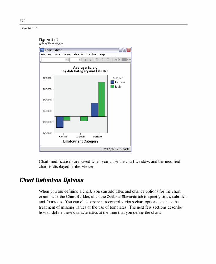
578

Chapter 41

Figure 41-7Modified chart

Chart modifications are saved when you close the chart window, and the modifiedchart is displayed in the Viewer.

Chart Definition Options

When you are defining a chart, you can add titles and change options for the chartcreation. In the Chart Builder, click the Optional Elements tab to specify titles, subtitles,and footnotes. You can click Options to control various chart options, such as thetreatment of missing values or the use of templates. The next few sections describehow to define these characteristics at the time that you define the chart.

579


Titles, Subtitles, and Footnotes

In any chart, you can define two title lines, one subtitle line, and two footnote lines aspart of your original chart definition. To specify titles or footnotes while defining achart, click the Optional Elements tab in the Chart Builder dialog box. Then drag one ofthe items to the canvas. You can modify the text that is associated with the item byclicking Element Properties and selecting the item from the Edit Properties of list.

Each line can be up to 72 characters. The number of characters that will actually fitin the chart depends on the font and size. Most titles are left-justified by default and,if too long, are cropped on the right. Pie chart titles, by default, are center-justifiedand, if too long, are cropped at both ends.

Titles, subtitles, and footnotes are rendered as text boxes in the Chart Editor. Withinthe Chart Editor, you can add, delete, or revise text boxes, as well as change theirfont, size, and justification.

Options

The Options dialog box provides options for the chart that you are creating. Thisdialog box is available by clicking Options.

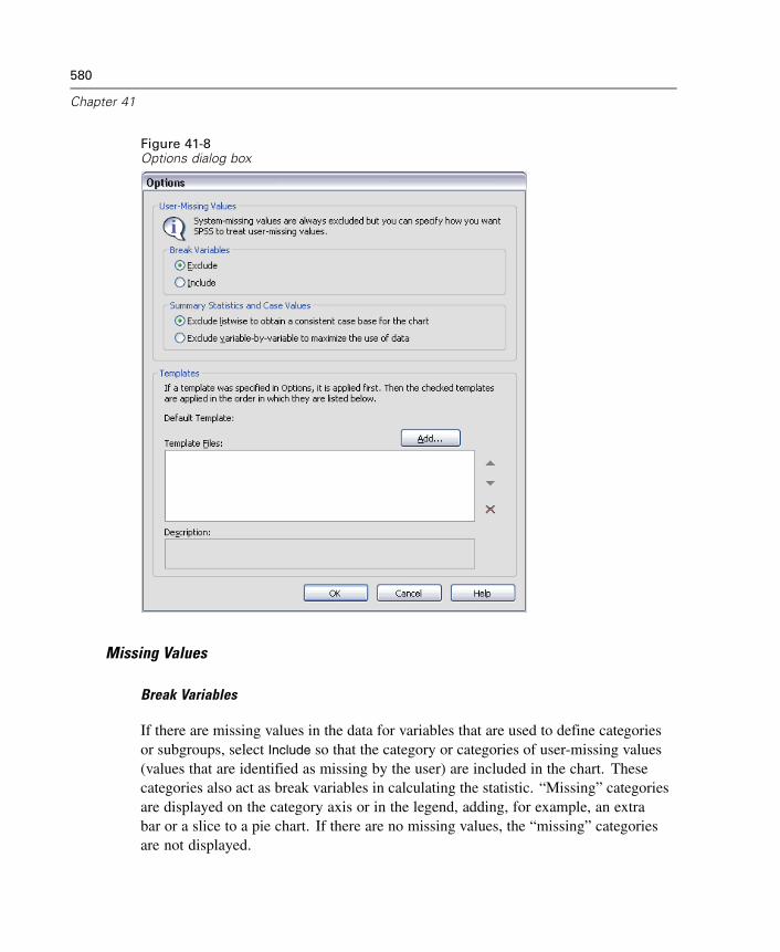
580

Chapter 41

Figure 41-8Options dialog box

Missing Values

Break Variables

If there are missing values in the data for variables that are used to define categoriesor subgroups, select Include so that the category or categories of user-missing values(values that are identified as missing by the user) are included in the chart. Thesecategories also act as break variables in calculating the statistic. “Missing” categoriesare displayed on the category axis or in the legend, adding, for example, an extrabar or a slice to a pie chart. If there are no missing values, the “missing” categoriesare not displayed.

581


If you select this option and want to suppress display after the chart is drawn, selectthe chart, and then choose Properties from the Edit menu. Click the Categories tab andmove the categories that you want suppressed to the Excluded list.

Summary Statistics and Case Values

You can choose one of the following alternatives to exclude cases that have missingvalues:

Exclude listwise to obtain a consistent case base for the chart. If any of the variablesin the chart has a missing value for a given case, the whole case is excluded fromthe chart.

Exclude variable-by-variable to maximize the use of data. If a selected variable hasany missing values, the cases that have those missing values are excluded whenthe variable is analyzed.

To see the difference between listwise and variable-by-variable exclusion of missingvalues, consider the following figures, which show a bar chart for each of the twooptions.

Figure 41-9Listwise exclusion of missing values

582

Chapter 41

Figure 41-10Variable-by-variable exclusion of missing values

The charts were created from a version of the Employee data.sav file that was edited tohave some system-missing (blank) values in the variables for current salary and jobcategory. In some other cases, the value 0 was entered and defined as missing. Forboth charts, the option Display groups defined by missing values is selected, which addsthe category Missing to the other displayed job categories. In each chart, the values ofthe summary function, Number of cases, are displayed in the bar labels.

In both charts, 26 cases have a system-missing value for the job category, and 13cases have the user-missing value (0). In the listwise chart, the number of cases is thesame for both variables in each bar cluster because whenever a value was missing, thecase was excluded for all variables. In the variable-by-variable chart, the number ofnonmissing cases for each variable in a category is plotted without regard to missingvalues in other variables.

Chart Templates

You can apply many of the attributes and text elements from one chart to another chart.This capability allows you to modify one chart, save that chart as a template, and thenuse the template to create a number of other similar charts.

583


To use a template when creating a chart, click Add in the Templates group. Thisopens a standard file selection dialog box. If you add multiple templates, the templatesare applied in the order in which they appear in Template Files list. You can changethe order if needed.

To apply a template to a chart that is already in the Chart Editor, from the menus choose:File

Apply Chart Template...

This opens a standard file selection dialog box. Select a file to use as a template. Ifyou are creating a new chart, the filename that you select is displayed in the Templategroup when you return to the chart definition dialog box.

A template borrows the format from one chart and applies it to the new chart that youare generating. In general, any formatting information from the old chart that can applyto the new chart will automatically apply. For example, if the old chart is a clustered barchart with bar colors modified to yellow and green, and the new chart is a multiple linechart, the lines will be yellow and green. If the old chart is a simple bar chart with dropshadows, and the new chart is a simple line chart, the lines will not have drop shadowsbecause drop shadows don’t apply to line charts. If there are titles in the template chartbut not in the new chart, you will get the titles from the template chart. If there aretitles defined in the new chart, they will override the titles in the template chart.

To Create a Chart Template

E Create a chart.

E Edit the chart to contain the attributes that you want to have in a template.

E From the Chart Editor menus choose:File

Save Chart Template...

E In the Save Chart Template dialog box, specify which characteristics of the chart youwant to save in the template. The online Help describes the settings in detail.

E Click Continue.

E Enter a filename and location for the new template. The template’s extension is .sgt.

Chapter

42ROC Curves

This procedure is a useful way to evaluate the performance of classification schemes inwhich there is one variable with two categories by which subjects are classified.

Example. It is in a bank’s interest to correctly classify customers into those customerswho will and will not default on their loans, so special methods are developed formaking these decisions. ROC curves can be used to evaluate how well these methodsperform.

Statistics. Area under the ROC curve with confidence interval and coordinate points ofthe ROC curve. Plots: ROC curve.

Methods. The estimate of the area under the ROC curve can be computed eithernonparametrically or parametrically using a binegative exponential model.

Data. Test variables are quantitative. Test variables are often composed of probabilitiesfrom discriminant analysis or logistic regression or composed of scores on an arbitraryscale indicating a rater’s “strength of conviction” that a subject falls into one categoryor another category. The state variable can be of any type and indicates the truecategory to which a subject belongs. The value of the state variable indicates whichcategory should be considered positive.

Assumptions. It is assumed that increasing numbers on the rater scale represent theincreasing belief that the subject belongs to one category, while decreasing numbers onthe scale represent the increasing belief that the subject belongs to the other category.The user must choose which direction is positive. It is also assumed that the truecategory to which each subject belongs is known.

585

586

Chapter 42

Figure 42-1ROC Curve output

Case ProcessingSummary

74

76

ACTUALPositive1

Negative

Valid N(listwise)

Larger values of the test result variable(s) indicatestronger evidence for a positive actual state.

The positive actual state is 1.00.1.

Area Under the Curve

Test Result Variable(s): PROBS

.877 .028 .000 .823 .931Area Std. Error1 Asymptotic Sig.2 Lower Bound Upper Bound

Asymptotic 95% ConfidenceInterval

Under the nonparametric assumption1.

Null hypothesis: true area = 0.52.

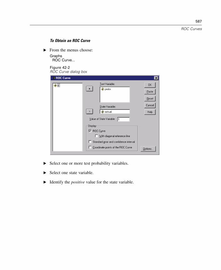
587

ROC Curves

To Obtain an ROC Curve

E From the menus choose:Graphs

ROC Curve...

Figure 42-2ROC Curve dialog box

E Select one or more test probability variables.

E Select one state variable.

E Identify the positive value for the state variable.

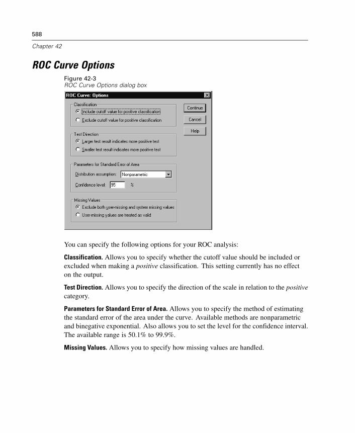
588

Chapter 42

ROC Curve OptionsFigure 42-3ROC Curve Options dialog box

You can specify the following options for your ROC analysis:

Classification. Allows you to specify whether the cutoff value should be included orexcluded when making a positive classification. This setting currently has no effecton the output.

Test Direction. Allows you to specify the direction of the scale in relation to the positivecategory.

Parameters for Standard Error of Area. Allows you to specify the method of estimatingthe standard error of the area under the curve. Available methods are nonparametricand binegative exponential. Also allows you to set the level for the confidence interval.The available range is 50.1% to 99.9%.

Missing Values. Allows you to specify how missing values are handled.

Chapter

43Utilities

This chapter describes the functions found on the Utilities menu and the ability toreorder target variable lists using the Windows system menus.

Variable Information

The Variables dialog box displays variable definition information for the currentlyselected variable, including:

Data format

Variable label

User-missing values

Value labels

Figure 43-1Variables dialog box

Go To. Goes to the selected variable in the Data Editor window.

589

590

Chapter 43

Paste. Pastes the selected variables into the designated syntax window at the cursorlocation.

To modify variable definitions, use the Variable view in the Data Editor.

To Obtain Variable Information


Variables...

E Select the variable for which you want to display variable definition information.

Data File Comments

You can include descriptive comments with a data file. For SPSS-format data files,these comments are saved with the data file.

To Add, Modify, Delete, or Display Data File Comments


Data File Comments...

E To display the comments in the Viewer, select Display comments in output.

Comments can be any length but are limited to 80 bytes (typically 80 charactersin single-byte languages) per line; lines will automatically wrap at 80 characters.Comments are displayed in the same font as text output to accurately reflect how theywill appear when displayed in the Viewer.

A date stamp (the current date in parentheses) is automatically appended to the endof the list of comments whenever you add or modify comments. This may lead to someambiguity concerning the dates associated with comments if you modify an existingcomment or insert a new comment between existing comments.

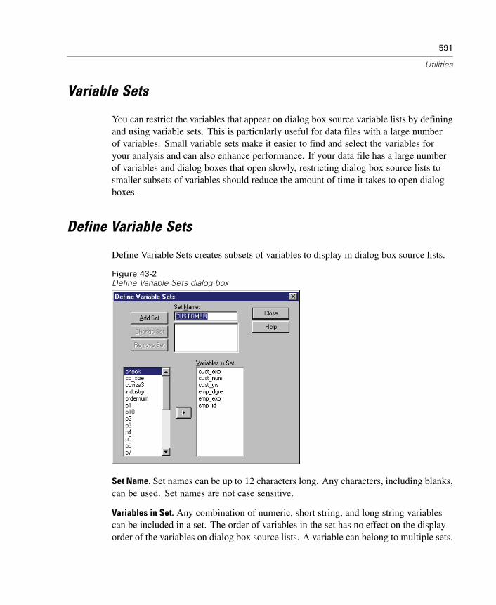
591

Utilities

Variable Sets

You can restrict the variables that appear on dialog box source variable lists by definingand using variable sets. This is particularly useful for data files with a large numberof variables. Small variable sets make it easier to find and select the variables foryour analysis and can also enhance performance. If your data file has a large numberof variables and dialog boxes that open slowly, restricting dialog box source lists tosmaller subsets of variables should reduce the amount of time it takes to open dialogboxes.

Define Variable Sets

Define Variable Sets creates subsets of variables to display in dialog box source lists.

Figure 43-2Define Variable Sets dialog box

Set Name. Set names can be up to 12 characters long. Any characters, including blanks,can be used. Set names are not case sensitive.

Variables in Set. Any combination of numeric, short string, and long string variablescan be included in a set. The order of variables in the set has no effect on the displayorder of the variables on dialog box source lists. A variable can belong to multiple sets.

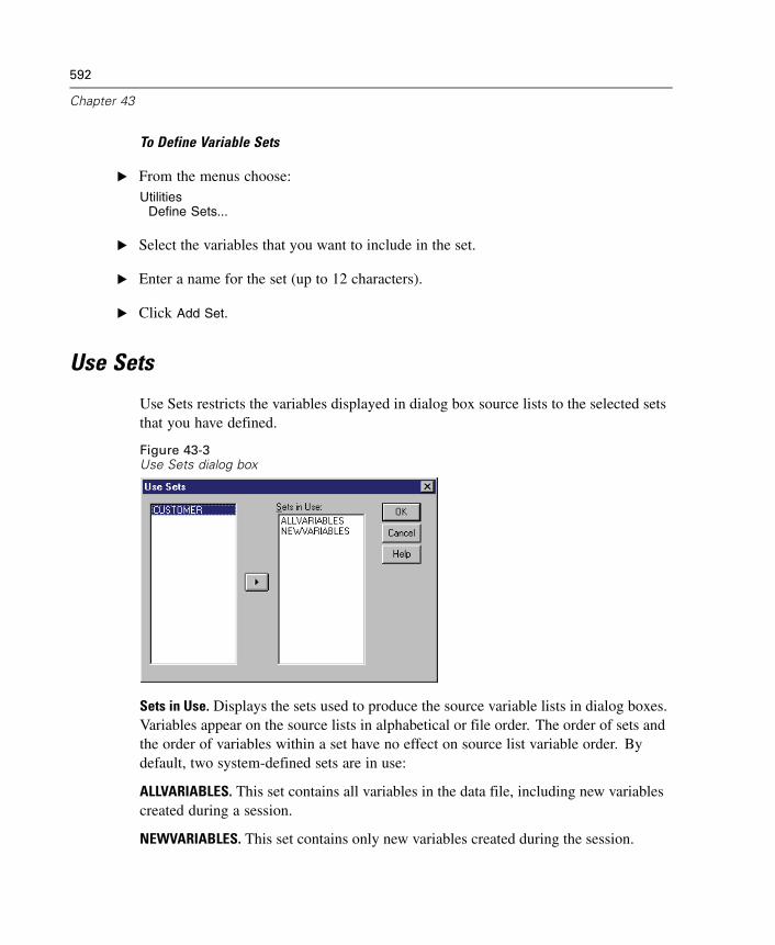
592

Chapter 43

To Define Variable Sets


Define Sets...

E Select the variables that you want to include in the set.

E Enter a name for the set (up to 12 characters).

E Click Add Set.

Use Sets

Use Sets restricts the variables displayed in dialog box source lists to the selected setsthat you have defined.

Figure 43-3Use Sets dialog box

Sets in Use. Displays the sets used to produce the source variable lists in dialog boxes.Variables appear on the source lists in alphabetical or file order. The order of sets andthe order of variables within a set have no effect on source list variable order. Bydefault, two system-defined sets are in use:

ALLVARIABLES. This set contains all variables in the data file, including new variablescreated during a session.

NEWVARIABLES. This set contains only new variables created during the session.

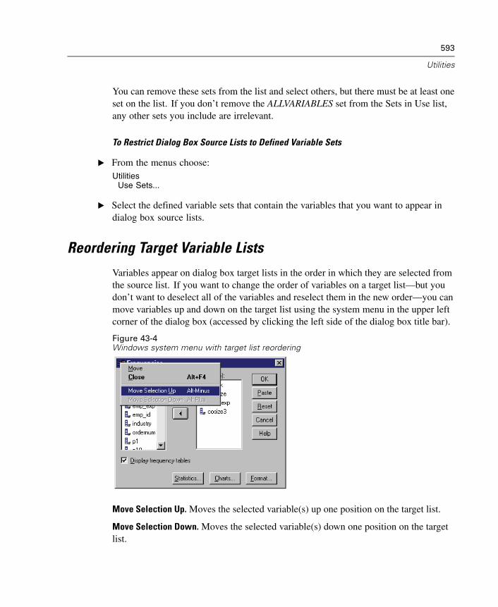
593

Utilities

You can remove these sets from the list and select others, but there must be at least oneset on the list. If you don’t remove the ALLVARIABLES set from the Sets in Use list,any other sets you include are irrelevant.

To Restrict Dialog Box Source Lists to Defined Variable Sets


Use Sets...

E Select the defined variable sets that contain the variables that you want to appear indialog box source lists.

Reordering Target Variable Lists

Variables appear on dialog box target lists in the order in which they are selected fromthe source list. If you want to change the order of variables on a target list—but youdon’t want to deselect all of the variables and reselect them in the new order—you canmove variables up and down on the target list using the system menu in the upper leftcorner of the dialog box (accessed by clicking the left side of the dialog box title bar).

Figure 43-4Windows system menu with target list reordering

Move Selection Up. Moves the selected variable(s) up one position on the target list.

Move Selection Down. Moves the selected variable(s) down one position on the targetlist.

594

Chapter 43

You can move multiple variables simultaneously if they are contiguous (groupedtogether). You cannot move noncontiguous groups of variables.

Chapter

44Options

Options control a wide variety of settings, including:

Session journal, which keeps a record of all commands run in every session

Display order for variables in dialog box source lists

Items displayed and hidden in new output results

TableLook for new pivot tables and ChartLook for new interactive charts

Custom currency formats

Autoscript files and autoscript functions to customize output

To Change Options Settings


Options...

E Click the tabs for the settings that you want to change.

E Change the settings.


595

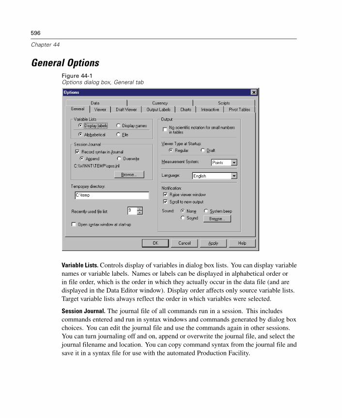
596

Chapter 44

General OptionsFigure 44-1Options dialog box, General tab

Variable Lists. Controls display of variables in dialog box lists. You can display variablenames or variable labels. Names or labels can be displayed in alphabetical order orin file order, which is the order in which they actually occur in the data file (and aredisplayed in the Data Editor window). Display order affects only source variable lists.Target variable lists always reflect the order in which variables were selected.

Session Journal. The journal file of all commands run in a session. This includescommands entered and run in syntax windows and commands generated by dialog boxchoices. You can edit the journal file and use the commands again in other sessions.You can turn journaling off and on, append or overwrite the journal file, and select thejournal filename and location. You can copy command syntax from the journal file andsave it in a syntax file for use with the automated Production Facility.

597

Options

Temporary directory. Controls the location of temporary files created during a session.In distributed mode (available with the server version), this does not affect the locationof temporary data files. In distributed mode, the location of temporary data files iscontrolled by the environment variable SPSSTMPDIR, which can be set only on thecomputer running the server version of the software. If you need to change the locationof the temporary directory, contact your system administrator.

Recently used file list. Controls the number of recently used files that appear on theFile menu.

Open syntax window at start-up. Syntax windows are text file windows used to enter,edit, and run commands. If you frequently work with command syntax, select thisoption to automatically open a syntax window at the beginning of each session. Thisis useful primarily for experienced users who prefer to work with command syntaxinstead of dialog boxes. (Not available with the Student Version.)

No scientific notation for small numbers in tables. Suppresses the display of scientificnotation for small decimal values in output. Very small decimal values will bedisplayed as 0 (or 0.000).

Viewer Type at Start-up. Controls the type of Viewer used and the output format. TheViewer produces interactive pivot tables and interactive charts. The Draft Viewerconverts pivot tables to text output and charts to metafiles.

Measurement System. The measurement system used (points, inches, or centimeters)for specifying attributes such as pivot table cell margins, cell widths, and spacebetween tables for printing.

Language. Controls the language used in the output. Does not apply to simple textoutput, interactive graphics, or maps (available with the Maps add-on module). The listof available languages depends on the currently installed language files.

Note: Custom scripts that rely on language-specific text strings in the output maynot run correctly when you change the output language. For more information, see“Script Options” on p. 613.

Notification. Controls the manner in which the program notifies you that it has finishedrunning a procedure and that the results are available in the Viewer.

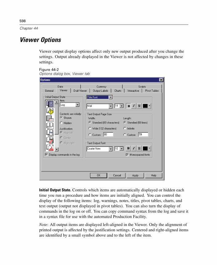
598

Chapter 44

Viewer Options

Viewer output display options affect only new output produced after you change thesettings. Output already displayed in the Viewer is not affected by changes in thesesettings.

Figure 44-2Options dialog box, Viewer tab

Initial Output State. Controls which items are automatically displayed or hidden eachtime you run a procedure and how items are initially aligned. You can control thedisplay of the following items: log, warnings, notes, titles, pivot tables, charts, andtext output (output not displayed in pivot tables). You can also turn the display ofcommands in the log on or off. You can copy command syntax from the log and save itin a syntax file for use with the automated Production Facility.

Note: All output items are displayed left-aligned in the Viewer. Only the alignment ofprinted output is affected by the justification settings. Centered and right-aligned itemsare identified by a small symbol above and to the left of the item.

599

Options

Title Font. Controls the font style, size, and color for new output titles.

Page Title Font. Controls the font style, size, and color for new page titles and pagetitles generated by TITLE and SUBTITLE command syntax or created by New Page

Title on the Insert menu.

Text Output Page Size. For text output, controls the page width (expressed in numberof characters) and page length (expressed in number of lines). For some procedures,some statistics are displayed only in wide format.

Text Output Font. Font used for text output. Text output is designed for use with amonospaced (fixed-pitch) font. If you select a non-monospaced font, tabular outputwill not align properly. The text output font is also used in the Text Wizard to displaythe file contents, which will not be aligned if the font is not monospaced.

Draft Viewer Options

Draft Viewer output display options affect only new output produced after you changethe settings. Output already displayed in the Draft Viewer is not affected by changes inthese settings.

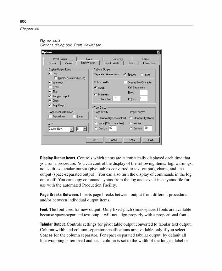
600

Chapter 44

Figure 44-3Options dialog box, Draft Viewer tab

Display Output Items. Controls which items are automatically displayed each time thatyou run a procedure. You can control the display of the following items: log, warnings,notes, titles, tabular output (pivot tables converted to text output), charts, and textoutput (space-separated output). You can also turn the display of commands in the logon or off. You can copy command syntax from the log and save it in a syntax file foruse with the automated Production Facility.

Page Breaks Between. Inserts page breaks between output from different proceduresand/or between individual output items.

Font. The font used for new output. Only fixed-pitch (monospaced) fonts are availablebecause space-separated text output will not align properly with a proportional font.

Tabular Output. Controls settings for pivot table output converted to tabular text output.Column width and column separator specifications are available only if you selectSpaces for the column separator. For space-separated tabular output, by default allline wrapping is removed and each column is set to the width of the longest label or

601

Options

value in the column. To limit the width of columns and wrap long labels, specify anumber of characters for the column width.

Note: Tab-separated tabular output will not align properly in the Draft Viewer. Thisformat is useful for copying and pasting results to word-processing applicationswhere you can use any font that you want (not only fixed-pitch fonts) and set the tabsto align output properly.

Text Output. For text output other than converted pivot table output, controls the pagewidth (expressed in number of characters) and page length (expressed in number oflines). For some procedures, some statistics are displayed only in wide format.

Output Label Options

Output label options control the display of variable and data value information in theoutline and pivot tables. You can display variable names, defined variable labels andactual data values, defined value labels, or a combination.

Descriptive variable and value labels (Variable view in the Data Editor, Label andValues columns) often make it easier to interpret your results. However, long labelscan be awkward in some tables.

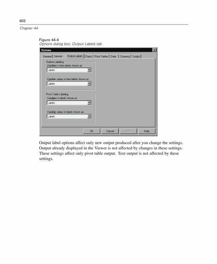
602

Chapter 44

Figure 44-4Options dialog box, Output Labels tab

Output label options affect only new output produced after you change the settings.Output already displayed in the Viewer is not affected by changes in these settings.These settings affect only pivot table output. Text output is not affected by thesesettings.

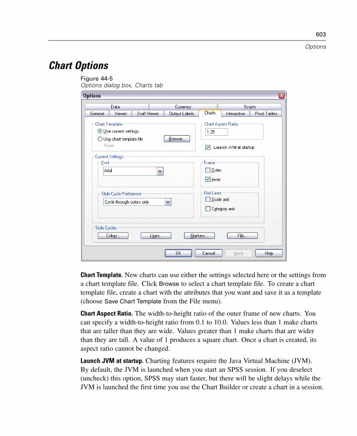
603

Options

Chart OptionsFigure 44-5Options dialog box, Charts tab

Chart Template. New charts can use either the settings selected here or the settings froma chart template file. Click Browse to select a chart template file. To create a charttemplate file, create a chart with the attributes that you want and save it as a template(choose Save Chart Template from the File menu).

Chart Aspect Ratio. The width-to-height ratio of the outer frame of new charts. Youcan specify a width-to-height ratio from 0.1 to 10.0. Values less than 1 make chartsthat are taller than they are wide. Values greater than 1 make charts that are widerthan they are tall. A value of 1 produces a square chart. Once a chart is created, itsaspect ratio cannot be changed.

Launch JVM at startup. Charting features require the Java Virtual Machine (JVM).By default, the JVM is launched when you start an SPSS session. If you deselect(uncheck) this option, SPSS may start faster, but there will be slight delays while theJVM is launched the first time you use the Chart Builder or create a chart in a session.

604

Chapter 44

Font. Font used for all text in new charts.

Style Cycle Preference. The initial assignment of colors and patterns for new charts.Cycle through colors only uses only colors to differentiate chart elements and does notuse patterns. Cycle through patterns only uses only line styles, marker symbols, or fillpatterns to differentiate chart elements and does not use color.

Frame. Controls the display of inner and outer frames on new charts.

Grid Lines. Controls the display of scale and category axis grid lines on new charts.

Style Cycles. Customizes the colors, line styles, marker symbols, and fill patterns fornew charts. You can change the order of the colors and patterns that are used whena new chart is created.

Note: These settings have no effect on interactive charts (the Graphs menu’s Interactivesubmenu).

Data Element Colors

Specify the order in which colors should be used for the data elements (such as bars andmarkers) in your new chart. Colors are used whenever you select a choice that includescolor in the Style Cycle Preference group in the main Chart Options dialog box.

For example, if you create a clustered bar chart with two groups and you selectCycle through colors, then patterns in the main Chart Options dialog box, the first twocolors in the Grouped Charts list are used as the bar colors on the new chart.

To Change the Order in Which Colors Are Used

E Select Simple Charts and then select a color that is used for charts without categories.

E Select Grouped Charts to change the color cycle for charts with categories. To changea category’s color, select a category and then select a color for that category fromthe palette.


Insert a new category above the selected category.

Move a selected category.

Remove a selected category.

605

Options

Reset the sequence to the default sequence.

Edit a color by selecting its well and then clicking Edit.

Data Element Lines

Specify the order in which styles should be used for the line data elements in yournew chart. Line styles are used whenever your chart includes line data elements andyou select a choice that includes patterns in the Style Cycle Preference group in themain Chart Options dialog box.

For example, if you create a line chart with two groups and you select Cycle through

patterns only in the main Chart Options dialog box, the first two styles in the GroupedCharts list are used as the line patterns on the new chart.

To Change the Order in Which Line Styles Are Used

E Select Simple Charts and then select a line style that is used for line charts withoutcategories.

E Select Grouped Charts to change the pattern cycle for line charts with categories. Tochange a category’s line style, select a category and then select a line style for thatcategory from the palette.






Data Element Markers

Specify the order in which symbols should be used for the marker data elements inyour new chart. Marker styles are used whenever your chart includes marker dataelements and you select a choice that includes patterns in the Style Cycle Preferencegroup in the main Chart Options dialog box.

606

Chapter 44

For example, if you create a scatterplot chart with two groups and you select Cycle

through patterns only in the main Chart Options dialog box, the first two symbols in theGrouped Charts list are used as the markers on the new chart.

To Change the Order in Which Marker Styles Are Used

E Select Simple Charts and then select a marker symbol that is used for charts withoutcategories.

E Select Grouped Charts to change the pattern cycle for charts with categories. Tochange a category’s marker symbol, select a category and then select a symbol forthat category from the palette.






Data Element Fills

Specify the order in which fill styles should be used for the bar and area data elementsin your new chart. Fill styles are used whenever your chart includes bar or area dataelements, and you select a choice that includes patterns in the Style Cycle Preferencegroup in the main Chart Options dialog box.

For example, if you create a clustered bar chart with two groups and you selectCycle through patterns only in the main Chart Options dialog box, the first two styles inthe Grouped Charts list are used as the bar fill patterns on the new chart.

To Change the Order in Which Fill Styles Are Used

E Select Simple Charts and then select a fill pattern that is used for charts withoutcategories.

E Select Grouped Charts to change the pattern cycle for charts with categories. Tochange a category’s fill pattern, select a category and then select a fill pattern forthat category from the palette.

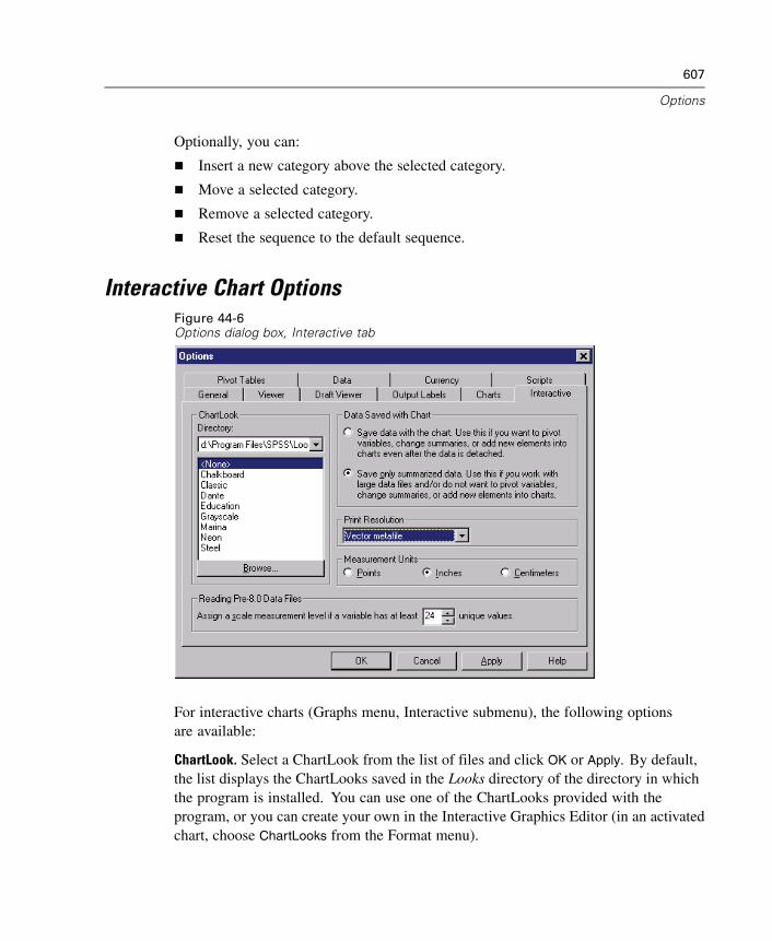
607

Options






Interactive Chart OptionsFigure 44-6Options dialog box, Interactive tab

For interactive charts (Graphs menu, Interactive submenu), the following optionsare available:

ChartLook. Select a ChartLook from the list of files and click OK or Apply. By default,the list displays the ChartLooks saved in the Looks directory of the directory in whichthe program is installed. You can use one of the ChartLooks provided with theprogram, or you can create your own in the Interactive Graphics Editor (in an activatedchart, choose ChartLooks from the Format menu).

608

Chapter 44

Directory. Allows you to select a ChartLook directory. Use Browse to adddirectories to the list.

Browse. Allows you to select a ChartLook from another directory.

Data Saved with Chart. Controls information saved with interactive charts once thecharts are no longer attached to the data file that created them (for example, if youopen a Viewer file saved in a previous session). Saving data with the chart enables youto perform most of the interactive functions available for charts attached to the datafile that created them (except adding variables that weren’t included in the originalchart). However, this can substantially increase the size of Viewer files, particularlyfor large data files.

Print Resolution. Controls the print resolution of interactive charts. In most cases, Vector

metafile will print faster and provide the best results. For bitmaps, lower resolutioncharts print faster; higher resolution charts look better.

Measurement Units. Measurement system used (points, inches, or centimeters) forspecifying attributes, such as the size of the data region in a chart.

Reading Pre-8.0 Data Files. For data files created in older versions of SPSS, data readfrom external file formats, and new variables created in a session, you can specify theminimum number of data values for a numeric variable used to classify the variableas scale or nominal. Variables with fewer than the specified number of unique valuesare classified as nominal.

Note: With the exception of measurement level, these settings affect only interactivecharts (the Graphs menu’s Interactive submenu).

Pivot Table Options

Pivot Table options sets the default TableLook used for new pivot table output.TableLooks can control a variety of pivot table attributes, including the display andwidth of grid lines; font style, size, and color; and background colors.

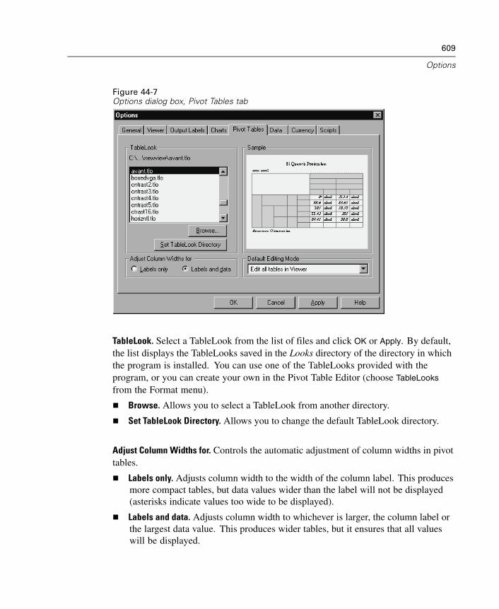
609

Options

Figure 44-7Options dialog box, Pivot Tables tab

TableLook. Select a TableLook from the list of files and click OK or Apply. By default,the list displays the TableLooks saved in the Looks directory of the directory in whichthe program is installed. You can use one of the TableLooks provided with theprogram, or you can create your own in the Pivot Table Editor (choose TableLooks

from the Format menu).

Browse. Allows you to select a TableLook from another directory.

Set TableLook Directory. Allows you to change the default TableLook directory.

Adjust Column Widths for. Controls the automatic adjustment of column widths in pivottables.

Labels only. Adjusts column width to the width of the column label. This producesmore compact tables, but data values wider than the label will not be displayed(asterisks indicate values too wide to be displayed).

Labels and data. Adjusts column width to whichever is larger, the column label orthe largest data value. This produces wider tables, but it ensures that all valueswill be displayed.

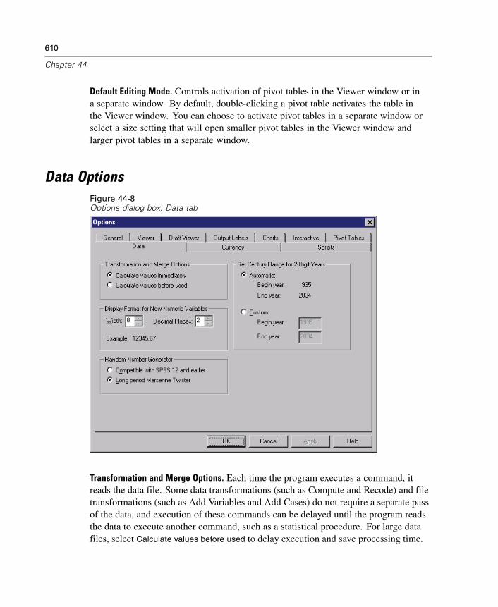
610

Chapter 44

Default Editing Mode. Controls activation of pivot tables in the Viewer window or ina separate window. By default, double-clicking a pivot table activates the table inthe Viewer window. You can choose to activate pivot tables in a separate window orselect a size setting that will open smaller pivot tables in the Viewer window andlarger pivot tables in a separate window.

Data OptionsFigure 44-8Options dialog box, Data tab

Transformation and Merge Options. Each time the program executes a command, itreads the data file. Some data transformations (such as Compute and Recode) and filetransformations (such as Add Variables and Add Cases) do not require a separate passof the data, and execution of these commands can be delayed until the program readsthe data to execute another command, such as a statistical procedure. For large datafiles, select Calculate values before used to delay execution and save processing time.

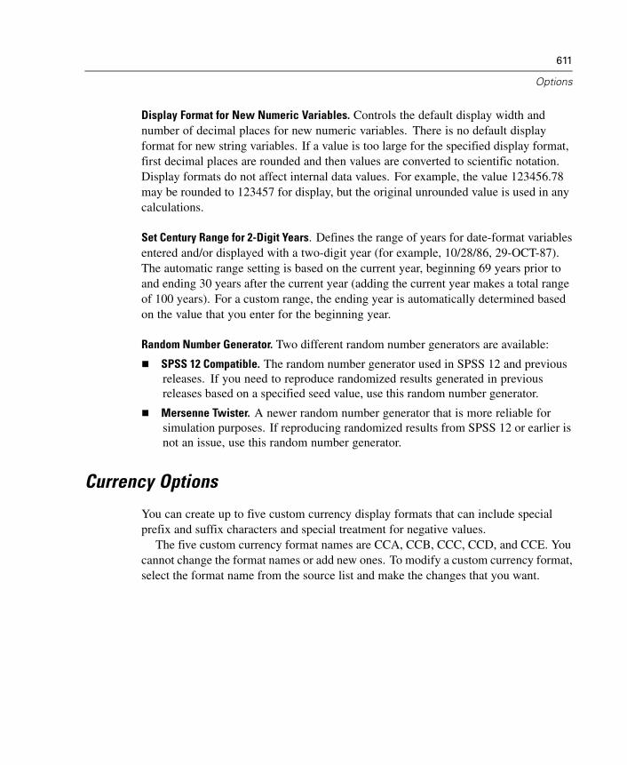
611

Options

Display Format for New Numeric Variables. Controls the default display width andnumber of decimal places for new numeric variables. There is no default displayformat for new string variables. If a value is too large for the specified display format,first decimal places are rounded and then values are converted to scientific notation.Display formats do not affect internal data values. For example, the value 123456.78may be rounded to 123457 for display, but the original unrounded value is used in anycalculations.

Set Century Range for 2-Digit Years. Defines the range of years for date-format variablesentered and/or displayed with a two-digit year (for example, 10/28/86, 29-OCT-87).The automatic range setting is based on the current year, beginning 69 years prior toand ending 30 years after the current year (adding the current year makes a total rangeof 100 years). For a custom range, the ending year is automatically determined basedon the value that you enter for the beginning year.

Random Number Generator. Two different random number generators are available:

SPSS 12 Compatible. The random number generator used in SPSS 12 and previousreleases. If you need to reproduce randomized results generated in previousreleases based on a specified seed value, use this random number generator.

Mersenne Twister. A newer random number generator that is more reliable forsimulation purposes. If reproducing randomized results from SPSS 12 or earlier isnot an issue, use this random number generator.

Currency Options

You can create up to five custom currency display formats that can include specialprefix and suffix characters and special treatment for negative values.

The five custom currency format names are CCA, CCB, CCC, CCD, and CCE. Youcannot change the format names or add new ones. To modify a custom currency format,select the format name from the source list and make the changes that you want.

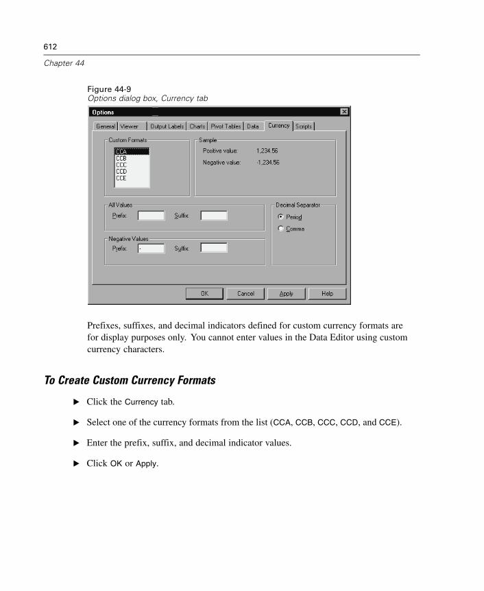
612

Chapter 44

Figure 44-9Options dialog box, Currency tab

Prefixes, suffixes, and decimal indicators defined for custom currency formats arefor display purposes only. You cannot enter values in the Data Editor using customcurrency characters.

To Create Custom Currency Formats

E Click the Currency tab.

E Select one of the currency formats from the list (CCA, CCB, CCC, CCD, and CCE).

E Enter the prefix, suffix, and decimal indicator values.


613

Options

Script Options

Use the Scripts tab to specify your global procedures file and autoscript file, and selectthe autoscript subroutines that you want to use. You can use scripts to automate manyfunctions, including customizing pivot tables.

Global Procedures. A global procedures file is a library of script subroutines andfunctions that can be called by script files, including autoscript files.

Note: The global procedures file that comes with the program is selected by default.Many of the available scripts use functions and subroutines in this global proceduresfile and will not work if you specify a different global procedures file.

Autoscripts. An autoscript file is a collection of script subroutines that run automaticallyeach time you run procedures that create certain types of output objects.

Figure 44-10Options dialog box, Scripts tab

All of the subroutines in the current autoscript file are displayed, allowing you toenable and disable individual subroutines.

614

Chapter 44

To Specify Global Procedure File and Autoscript File

E Click the Scripts tab.

E Select Enable Autoscripting.

E Select the autoscript subroutines that you want to enable.

You can also specify a different autoscript file or global procedure file.

Chapter

45Customizing Menus and Toolbars

Menu Editor

You can use the Menu Editor to customize your menus. With the Menu Editor you can:

Add menu items that run customized scripts.

Add menu items that run command syntax files.

Add menu items that launch other applications and automatically send data toother applications.

You can send data to other applications in the following formats: SPSS, Excel 4.0,Lotus 1-2-3 release 3, SYLK, tab-delimited, and dBASE IV.

To Add Items to Menus


Menu Editor...

E In the Menu Editor dialog box, double-click the menu to which you want to add anew item.

E Select the menu item above which you want the new item to appear.

E Click Insert Item to insert a new menu item.

E Select the file type for the new item (script file, command syntax file, or externalapplication).

E Click Browse to select a file to attach to the menu item.

615

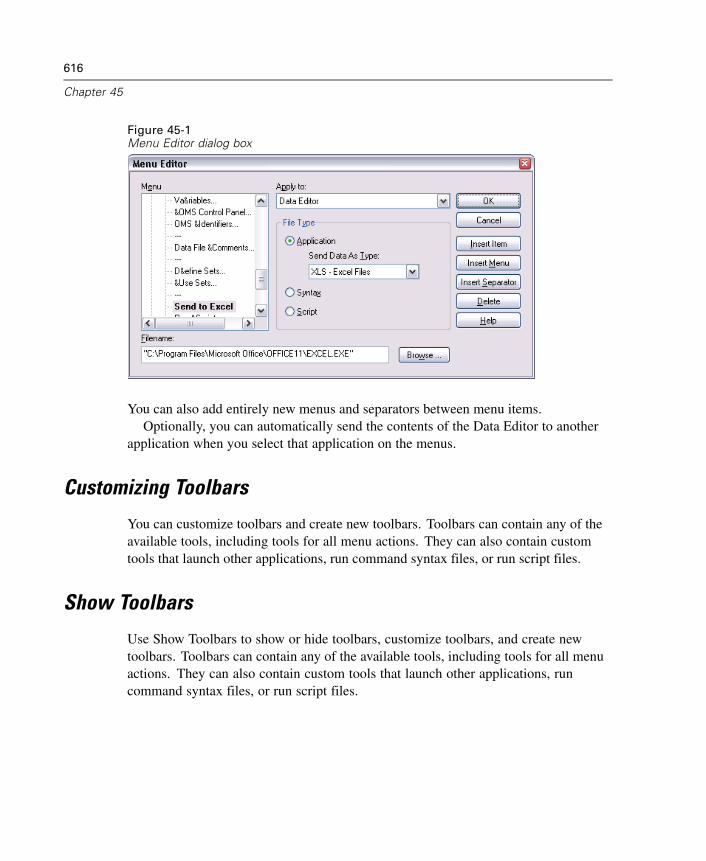
616

Chapter 45

Figure 45-1Menu Editor dialog box

You can also add entirely new menus and separators between menu items.Optionally, you can automatically send the contents of the Data Editor to another

application when you select that application on the menus.

Customizing Toolbars

You can customize toolbars and create new toolbars. Toolbars can contain any of theavailable tools, including tools for all menu actions. They can also contain customtools that launch other applications, run command syntax files, or run script files.

Show Toolbars

Use Show Toolbars to show or hide toolbars, customize toolbars, and create newtoolbars. Toolbars can contain any of the available tools, including tools for all menuactions. They can also contain custom tools that launch other applications, runcommand syntax files, or run script files.

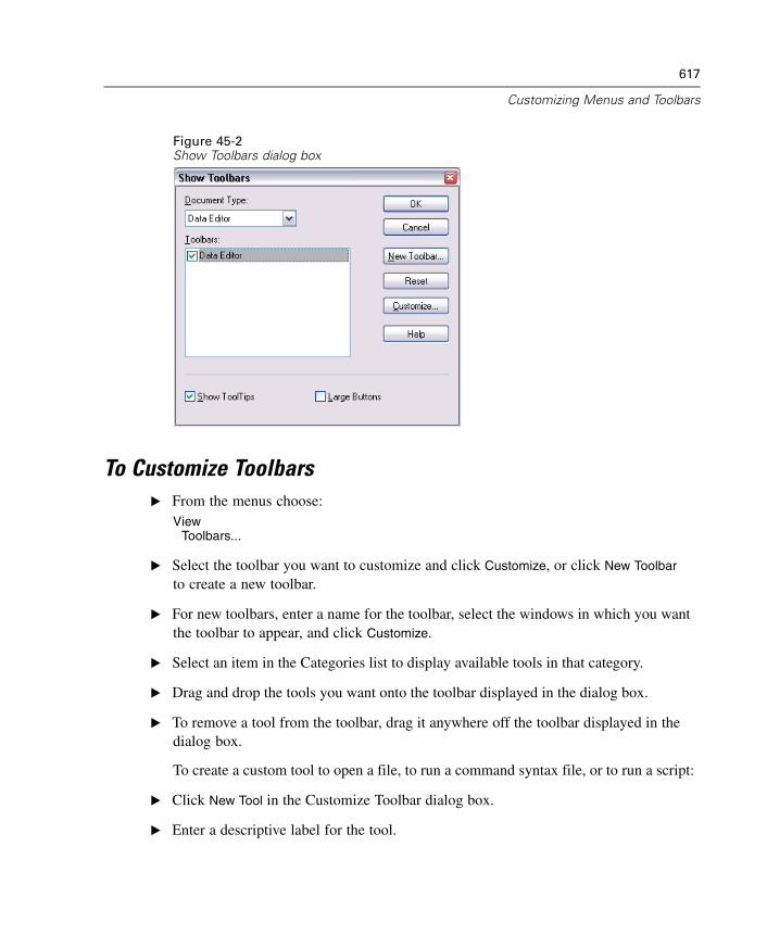
617

Customizing Menus and Toolbars

Figure 45-2Show Toolbars dialog box

To Customize ToolbarsE From the menus choose:

ViewToolbars...

E Select the toolbar you want to customize and click Customize, or click New Toolbar

to create a new toolbar.

E For new toolbars, enter a name for the toolbar, select the windows in which you wantthe toolbar to appear, and click Customize.

E Select an item in the Categories list to display available tools in that category.

E Drag and drop the tools you want onto the toolbar displayed in the dialog box.

E To remove a tool from the toolbar, drag it anywhere off the toolbar displayed in thedialog box.

To create a custom tool to open a file, to run a command syntax file, or to run a script:

E Click New Tool in the Customize Toolbar dialog box.

E Enter a descriptive label for the tool.

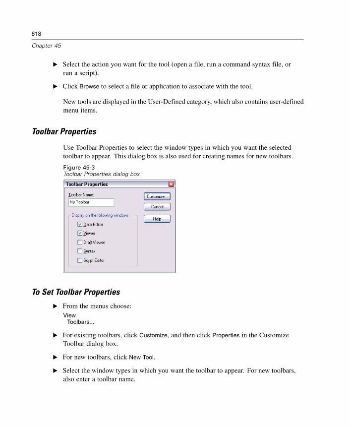
618

Chapter 45

E Select the action you want for the tool (open a file, run a command syntax file, orrun a script).

E Click Browse to select a file or application to associate with the tool.

New tools are displayed in the User-Defined category, which also contains user-definedmenu items.

Toolbar Properties

Use Toolbar Properties to select the window types in which you want the selectedtoolbar to appear. This dialog box is also used for creating names for new toolbars.

Figure 45-3Toolbar Properties dialog box

To Set Toolbar Properties


Toolbars...

E For existing toolbars, click Customize, and then click Properties in the CustomizeToolbar dialog box.

E For new toolbars, click New Tool.

E Select the window types in which you want the toolbar to appear. For new toolbars,also enter a toolbar name.

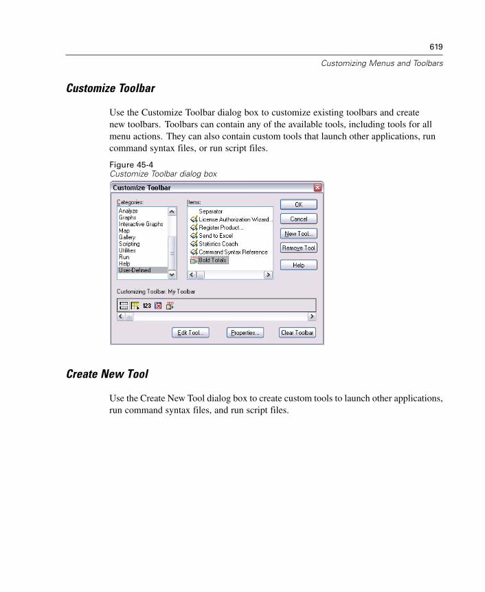
619


Customize Toolbar

Use the Customize Toolbar dialog box to customize existing toolbars and createnew toolbars. Toolbars can contain any of the available tools, including tools for allmenu actions. They can also contain custom tools that launch other applications, runcommand syntax files, or run script files.

Figure 45-4Customize Toolbar dialog box

Create New Tool

Use the Create New Tool dialog box to create custom tools to launch other applications,run command syntax files, and run script files.

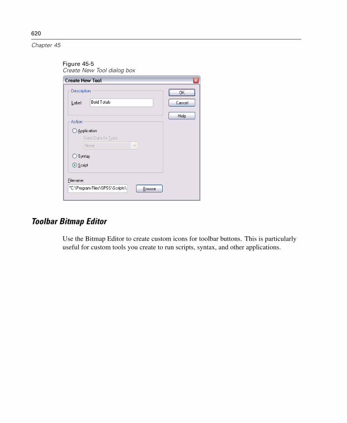
620

Chapter 45

Figure 45-5Create New Tool dialog box

Toolbar Bitmap Editor

Use the Bitmap Editor to create custom icons for toolbar buttons. This is particularlyuseful for custom tools you create to run scripts, syntax, and other applications.

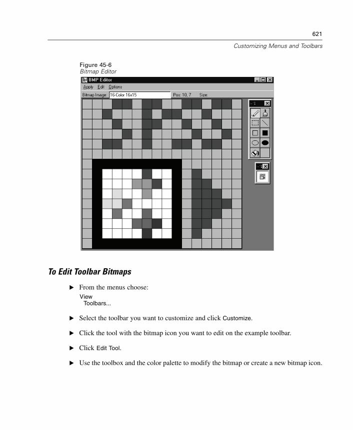
621


Figure 45-6Bitmap Editor

To Edit Toolbar Bitmaps


Toolbars...

E Select the toolbar you want to customize and click Customize.

E Click the tool with the bitmap icon you want to edit on the example toolbar.

E Click Edit Tool.

E Use the toolbox and the color palette to modify the bitmap or create a new bitmap icon.

Chapter

46Production Facility

The Production Facility provides the ability to run the program in an automatedfashion. The program runs unattended and terminates after executing the lastcommand, so you can perform other tasks while it runs. Production mode is useful ifyou often run the same set of time-consuming analyses, such as weekly reports.

The Production Facility uses command syntax files to tell the program what to do.A command syntax file is a simple text file containing command syntax. You can useany text editor to create the file. You can also generate command syntax by pastingdialog box selections into a syntax window or by editing the journal file.

After you create syntax files and include them in a production job, you can view andedit them from the Production Facility.

623

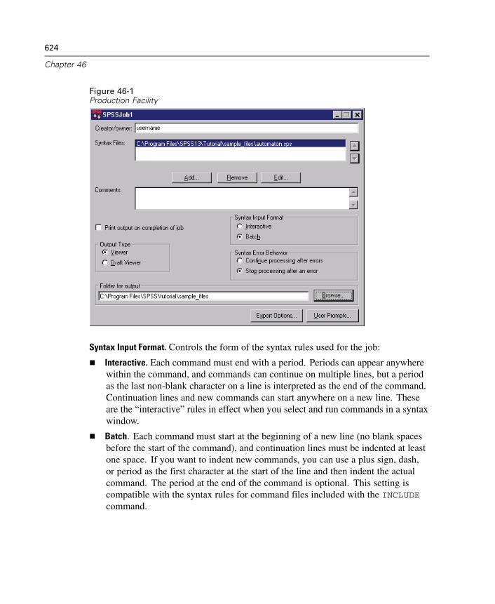
624

Chapter 46

Figure 46-1Production Facility

Syntax Input Format. Controls the form of the syntax rules used for the job:

Interactive. Each command must end with a period. Periods can appear anywherewithin the command, and commands can continue on multiple lines, but a periodas the last non-blank character on a line is interpreted as the end of the command.Continuation lines and new commands can start anywhere on a new line. Theseare the “interactive” rules in effect when you select and run commands in a syntaxwindow.

Batch. Each command must start at the beginning of a new line (no blank spacesbefore the start of the command), and continuation lines must be indented at leastone space. If you want to indent new commands, you can use a plus sign, dash,or period as the first character at the start of the line and then indent the actualcommand. The period at the end of the command is optional. This setting iscompatible with the syntax rules for command files included with the INCLUDEcommand.

625

Production Facility

Syntax Error Behavior. Controls the treatment of error conditions in the job:

Continue. Errors in the job do not automatically stop command processing. Thecommands in the production job files are treated as part of the normal commandstream, and command processing continues in the normal fashion.

Stop. Command processing stops when the first error in a production job file isencountered. This is compatible with the behavior of command files includedwith the INCLUDE command.

Production job results. Each production run creates an output file with the same nameas the production job and the extension .spo. For example, a production job filenamed prodjob.spp creates an output file named prodjob.spo. The output file is aViewer document.

Output Type. Viewer output produces pivot tables and high-resolution, interactive charts.Draft Viewer output produces text output and metafile pictures of charts. Text outputcan be edited in the Draft Viewer, but charts cannot be edited in the Draft Viewer.

Using the Production Facility

E Create a command syntax file.

E Start the Production Facility, available on the Start menu.

E Specify the syntax files that you want to use in the production job. Click Add to selectthe syntax files.

E Save the production job file.

E Run the production job file. Click the Run button on the toolbar, or from the menuschoose:Run

Production Job

Export Options

Export Options saves pivot tables and text output in HTML, text, Word/RTF, and Excelformat, and it saves charts in a variety of common formats used by other applications.

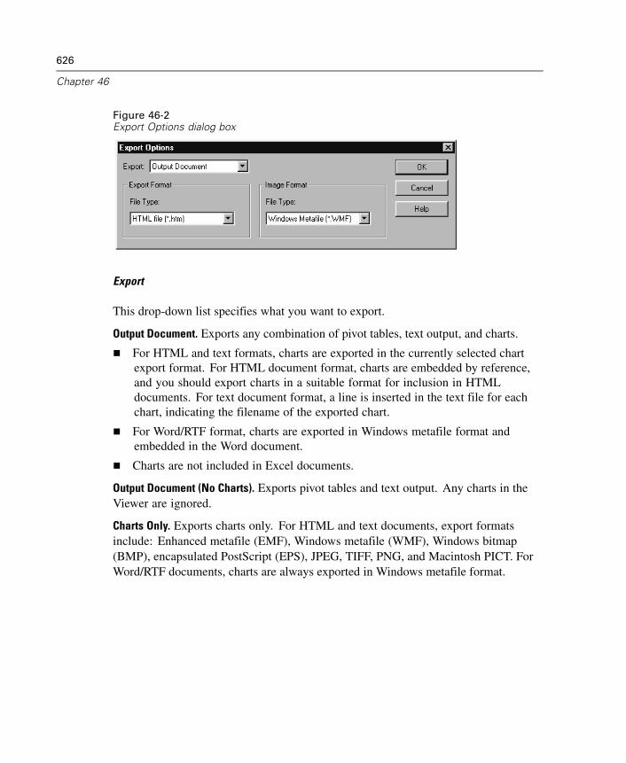
626

Chapter 46

Figure 46-2Export Options dialog box

Export

This drop-down list specifies what you want to export.

Output Document. Exports any combination of pivot tables, text output, and charts.

For HTML and text formats, charts are exported in the currently selected chartexport format. For HTML document format, charts are embedded by reference,and you should export charts in a suitable format for inclusion in HTMLdocuments. For text document format, a line is inserted in the text file for eachchart, indicating the filename of the exported chart.

For Word/RTF format, charts are exported in Windows metafile format andembedded in the Word document.

Charts are not included in Excel documents.

Output Document (No Charts). Exports pivot tables and text output. Any charts in theViewer are ignored.

Charts Only. Exports charts only. For HTML and text documents, export formatsinclude: Enhanced metafile (EMF), Windows metafile (WMF), Windows bitmap(BMP), encapsulated PostScript (EPS), JPEG, TIFF, PNG, and Macintosh PICT. ForWord/RTF documents, charts are always exported in Windows metafile format.

627

Production Facility

Export Format

For output documents, the available options are HTML, text, Word/RTF, and Excel;for HTML and text formats, charts are exported in the currently selected chart format.For Charts Only, select a chart export format from the drop-down list. For outputdocuments, pivot tables and text are exported in the following manner:

HTML file (*.htm). Pivot tables are exported as HTML tables. Text output is exportedas preformatted HTML.

Text file (*.txt). Pivot tables can be exported in tab-separated or space-separatedformat. All text output is exported in space-separated format.

Excel file (*.xls). Pivot table rows, columns, and cells are exported as Excel rows,columns, and cells, with all formatting attributes intact—for example, cell borders,font styles, background colors, and so on. Text output is exported with all fontattributes intact. Each line in the text output is a row in the Excel file, with theentire contents of the line contained in a single cell.

Word/RTF file (*.doc). Pivot tables are exported as Word tables with all formattingattributes intact—for example, cell borders, font styles, background colors, andso on. Text output is exported as formatted RTF. Text output in SPSS is alwaysdisplayed in a fixed-pitch (monospaced) font and is exported with the same fontattributes. A fixed-pitch font is required for proper alignment of space-separatedtext output.

Image Format

Image Format controls the export format for charts. Charts can be exported in thefollowing formats: Enhanced metafile (EMF), Windows metafile (WMF), Windowsbitmap (BMP), encapsulated PostScript (EPS), JPEG, TIFF, PNG, or Macintosh PICT.

Exported chart names are based on the production job filename, a sequentialnumber, and the extension of the selected format. For example, if the production jobprodjob.spp exports charts in Windows metafile format, the chart names would beprodjob1.wmf, prodjob2.wmf, prodjob3.wmf, and so on.

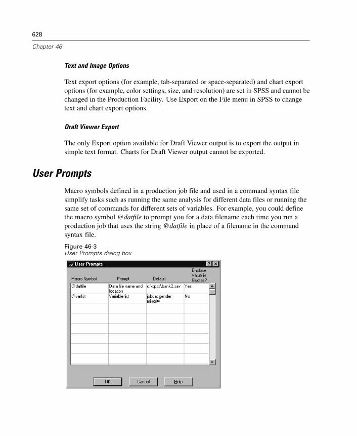
628

Chapter 46

Text and Image Options

Text export options (for example, tab-separated or space-separated) and chart exportoptions (for example, color settings, size, and resolution) are set in SPSS and cannot bechanged in the Production Facility. Use Export on the File menu in SPSS to changetext and chart export options.

Draft Viewer Export

The only Export option available for Draft Viewer output is to export the output insimple text format. Charts for Draft Viewer output cannot be exported.

User PromptsMacro symbols defined in a production job file and used in a command syntax filesimplify tasks such as running the same analysis for different data files or running thesame set of commands for different sets of variables. For example, you could definethe macro symbol @datfile to prompt you for a data filename each time you run aproduction job that uses the string @datfile in place of a filename in the commandsyntax file.

Figure 46-3User Prompts dialog box

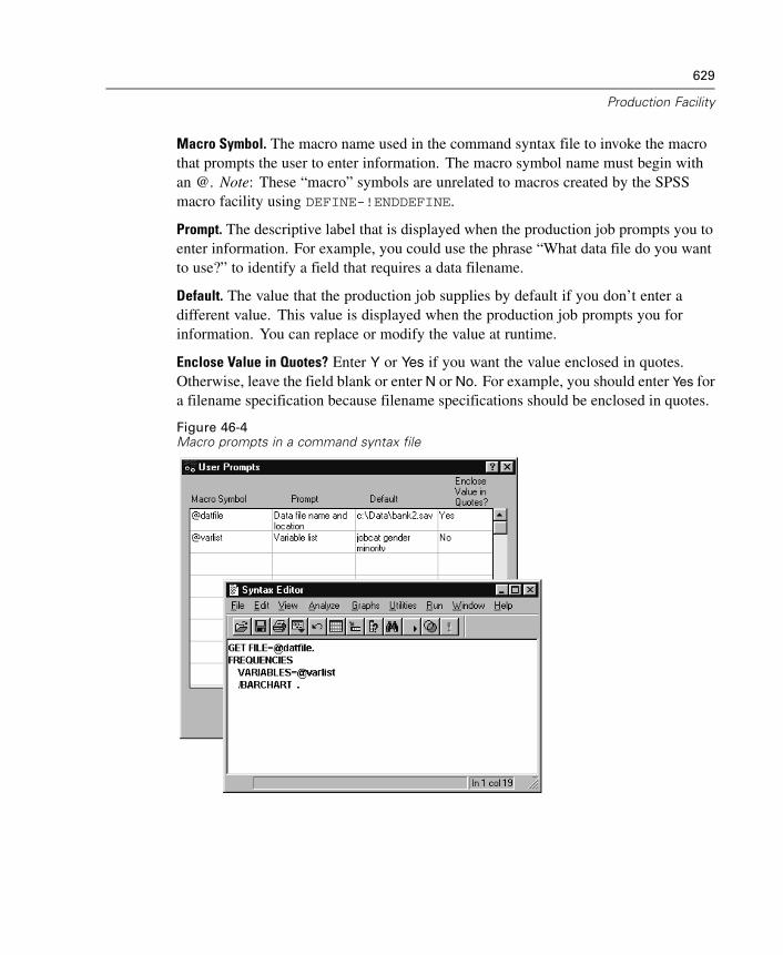
629

Production Facility

Macro Symbol. The macro name used in the command syntax file to invoke the macrothat prompts the user to enter information. The macro symbol name must begin withan @. Note: These “macro” symbols are unrelated to macros created by the SPSSmacro facility using DEFINE-!ENDDEFINE.

Prompt. The descriptive label that is displayed when the production job prompts you toenter information. For example, you could use the phrase “What data file do you wantto use?” to identify a field that requires a data filename.

Default. The value that the production job supplies by default if you don’t enter adifferent value. This value is displayed when the production job prompts you forinformation. You can replace or modify the value at runtime.

Enclose Value in Quotes? Enter Y or Yes if you want the value enclosed in quotes.Otherwise, leave the field blank or enter N or No. For example, you should enter Yes fora filename specification because filename specifications should be enclosed in quotes.

Figure 46-4Macro prompts in a command syntax file

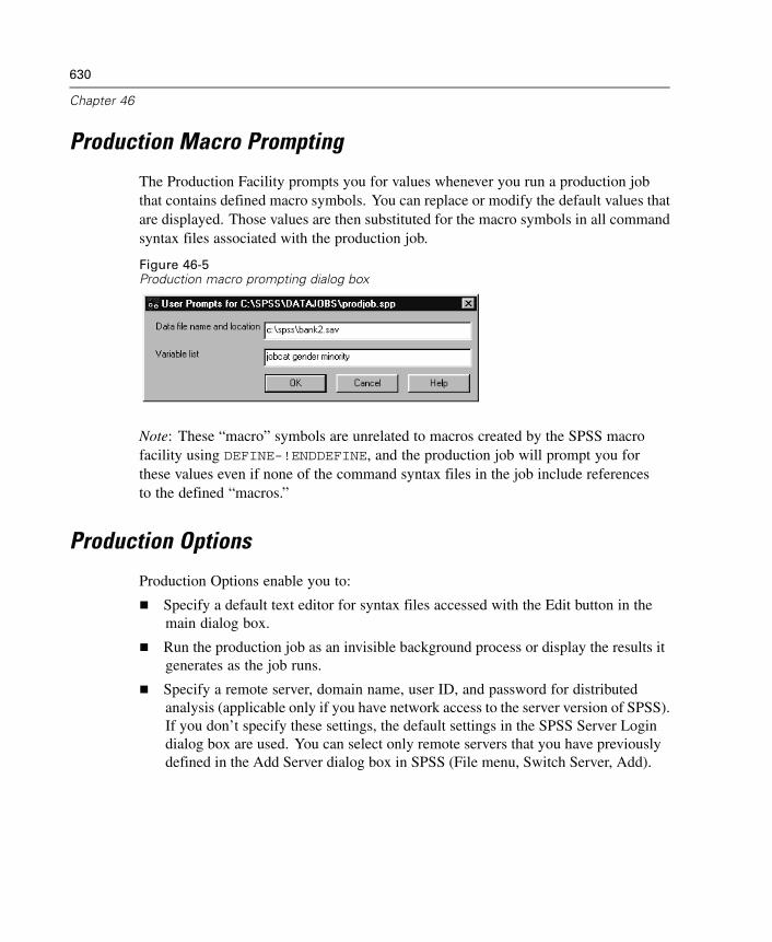
630

Chapter 46

Production Macro Prompting

The Production Facility prompts you for values whenever you run a production jobthat contains defined macro symbols. You can replace or modify the default values thatare displayed. Those values are then substituted for the macro symbols in all commandsyntax files associated with the production job.

Figure 46-5Production macro prompting dialog box

Note: These “macro” symbols are unrelated to macros created by the SPSS macrofacility using DEFINE-!ENDDEFINE, and the production job will prompt you forthese values even if none of the command syntax files in the job include referencesto the defined “macros.”

Production Options

Production Options enable you to:

Specify a default text editor for syntax files accessed with the Edit button in themain dialog box.

Run the production job as an invisible background process or display the results itgenerates as the job runs.

Specify a remote server, domain name, user ID, and password for distributedanalysis (applicable only if you have network access to the server version of SPSS).If you don’t specify these settings, the default settings in the SPSS Server Logindialog box are used. You can select only remote servers that you have previouslydefined in the Add Server dialog box in SPSS (File menu, Switch Server, Add).

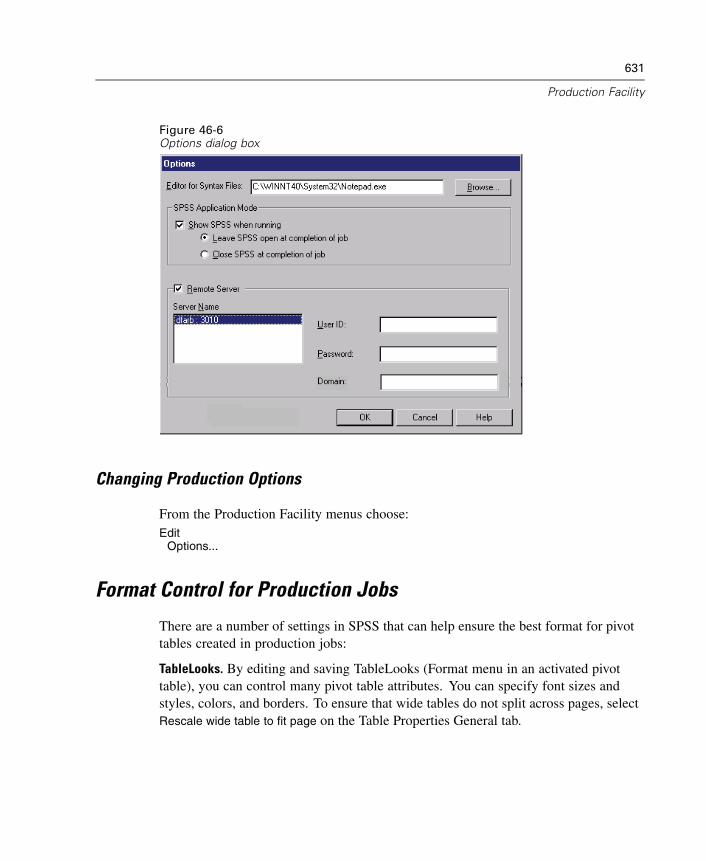
631

Production Facility

Figure 46-6Options dialog box

Changing Production Options

From the Production Facility menus choose:Edit

Options...

Format Control for Production Jobs

There are a number of settings in SPSS that can help ensure the best format for pivottables created in production jobs:

TableLooks. By editing and saving TableLooks (Format menu in an activated pivottable), you can control many pivot table attributes. You can specify font sizes andstyles, colors, and borders. To ensure that wide tables do not split across pages, selectRescale wide table to fit page on the Table Properties General tab.

632

Chapter 46

Output labels. Output label options (Edit menu, Options, Output Labels tab) control thedisplay of variable and data value information in pivot tables. You can display variablenames and/or defined variable labels, actual data values and/or defined value labels.Descriptive variable and value labels often make it easier to interpret your results;however, long labels can be awkward in some tables.

Column width. Pivot table options (Edit menu, Options, Pivot Table tab) control thedefault TableLook and the automatic adjustment of column widths in pivot tables.

Labels only. Adjusts the column width to the width of the column label. Thisproduces more compact tables, but data values wider than the label will not bedisplayed (asterisks indicate values too wide to be displayed).

Labels and data. Adjusts the column width to whichever is larger, the column labelor the largest data value. This produces wider tables, but it ensures that all valueswill be displayed.

Production jobs use the current TableLook and Options settings in effect. You can setthe TableLook and Options settings before running your production job, or you can useSET commands in your syntax files to control them. Using SET commands in syntaxfiles enables you to use multiple TableLooks and Options settings in the same job.

Creating a Custom Default TableLook

E Activate a pivot table (double-click anywhere in the table).


TableLook...

E Select a TableLook from the list and click Edit Look.

E Adjust the table properties for the attributes that you want.

E Click Save Look or Save As to save the TableLook and click OK.


Options...

E Click the Pivot Tables tab.

E Select the TableLook from the list and click OK.

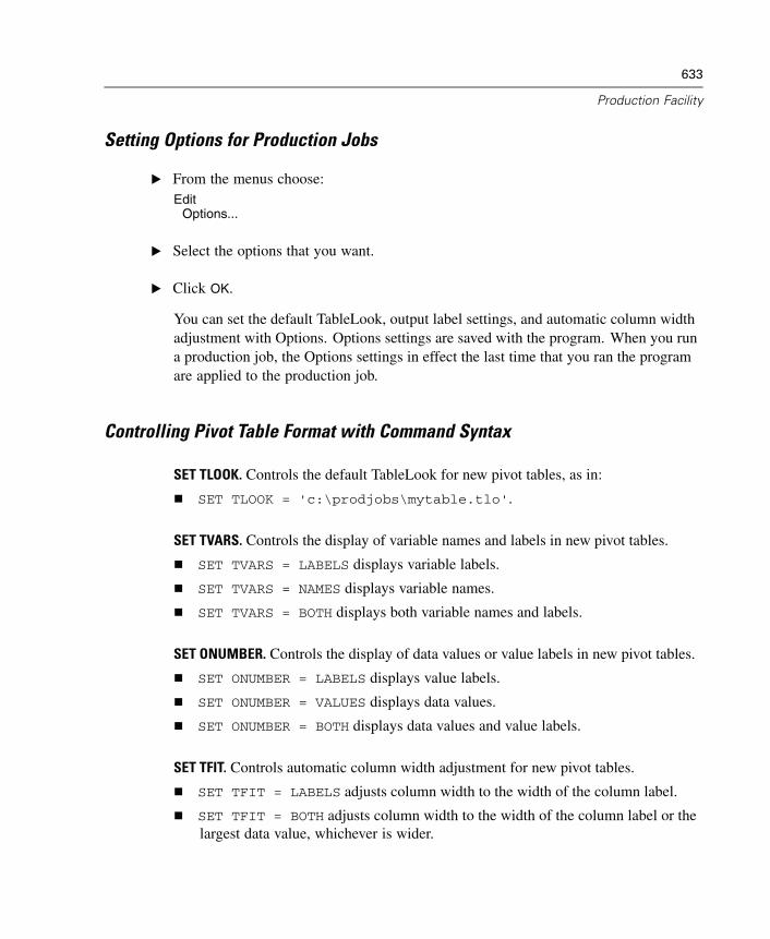
633

Production Facility

Setting Options for Production Jobs


Options...


E Click OK.

You can set the default TableLook, output label settings, and automatic column widthadjustment with Options. Options settings are saved with the program. When you runa production job, the Options settings in effect the last time that you ran the programare applied to the production job.

Controlling Pivot Table Format with Command Syntax

SET TLOOK. Controls the default TableLook for new pivot tables, as in:

SET TLOOK = 'c:\prodjobs\mytable.tlo'.

SET TVARS. Controls the display of variable names and labels in new pivot tables.

SET TVARS = LABELS displays variable labels.

SET TVARS = NAMES displays variable names.

SET TVARS = BOTH displays both variable names and labels.

SET ONUMBER. Controls the display of data values or value labels in new pivot tables.

SET ONUMBER = LABELS displays value labels.

SET ONUMBER = VALUES displays data values.

SET ONUMBER = BOTH displays data values and value labels.

SET TFIT. Controls automatic column width adjustment for new pivot tables.

SET TFIT = LABELS adjusts column width to the width of the column label.

SET TFIT = BOTH adjusts column width to the width of the column label or thelargest data value, whichever is wider.

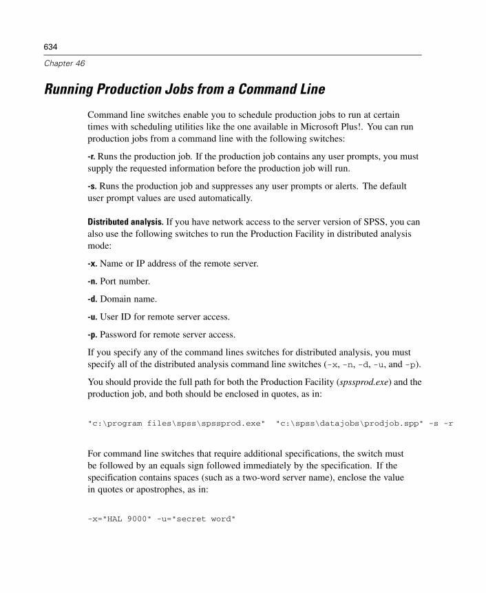
634

Chapter 46

Running Production Jobs from a Command Line

Command line switches enable you to schedule production jobs to run at certaintimes with scheduling utilities like the one available in Microsoft Plus!. You can runproduction jobs from a command line with the following switches:

-r. Runs the production job. If the production job contains any user prompts, you mustsupply the requested information before the production job will run.

-s. Runs the production job and suppresses any user prompts or alerts. The defaultuser prompt values are used automatically.

Distributed analysis. If you have network access to the server version of SPSS, you canalso use the following switches to run the Production Facility in distributed analysismode:

-x. Name or IP address of the remote server.

-n. Port number.

-d. Domain name.

-u. User ID for remote server access.

-p. Password for remote server access.

If you specify any of the command lines switches for distributed analysis, you mustspecify all of the distributed analysis command line switches (-x, -n, -d, -u, and -p).

You should provide the full path for both the Production Facility (spssprod.exe) and theproduction job, and both should be enclosed in quotes, as in:

"c:\program files\spss\spssprod.exe" "c:\spss\datajobs\prodjob.spp" -s -r

For command line switches that require additional specifications, the switch mustbe followed by an equals sign followed immediately by the specification. If thespecification contains spaces (such as a two-word server name), enclose the valuein quotes or apostrophes, as in:

-x="HAL 9000" -u="secret word"

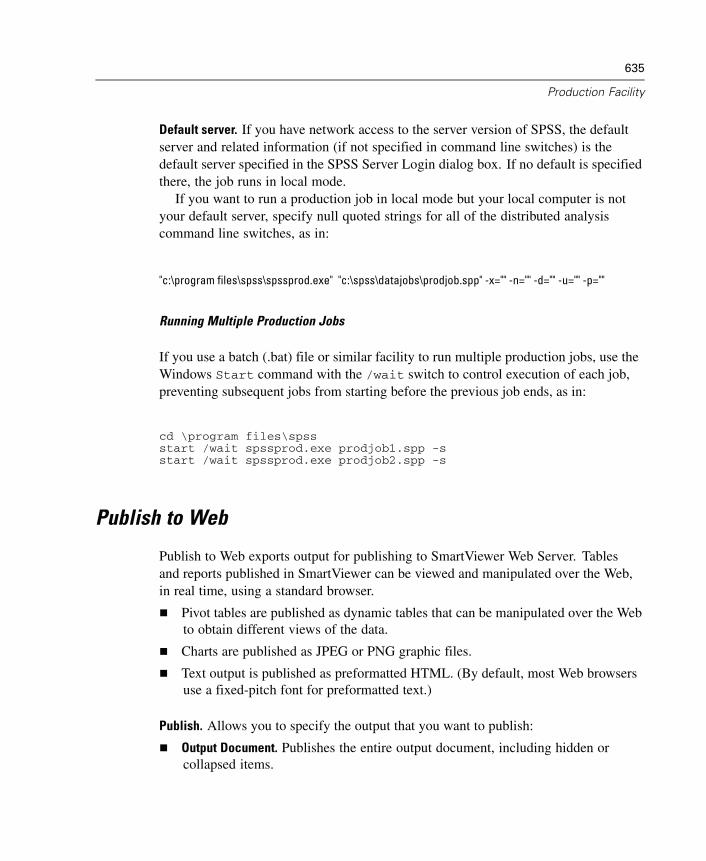
635

Production Facility

Default server. If you have network access to the server version of SPSS, the defaultserver and related information (if not specified in command line switches) is thedefault server specified in the SPSS Server Login dialog box. If no default is specifiedthere, the job runs in local mode.

If you want to run a production job in local mode but your local computer is notyour default server, specify null quoted strings for all of the distributed analysiscommand line switches, as in:

"c:\program files\spss\spssprod.exe" "c:\spss\datajobs\prodjob.spp" -x="" -n="" -d="" -u="" -p=""

Running Multiple Production Jobs

If you use a batch (.bat) file or similar facility to run multiple production jobs, use theWindows Start command with the /wait switch to control execution of each job,preventing subsequent jobs from starting before the previous job ends, as in:

cd \program files\spssstart /wait spssprod.exe prodjob1.spp -sstart /wait spssprod.exe prodjob2.spp -s

Publish to Web

Publish to Web exports output for publishing to SmartViewer Web Server. Tablesand reports published in SmartViewer can be viewed and manipulated over the Web,in real time, using a standard browser.

Pivot tables are published as dynamic tables that can be manipulated over the Webto obtain different views of the data.

Charts are published as JPEG or PNG graphic files.

Text output is published as preformatted HTML. (By default, most Web browsersuse a fixed-pitch font for preformatted text.)

Publish. Allows you to specify the output that you want to publish:

Output Document. Publishes the entire output document, including hidden orcollapsed items.

636

Chapter 46

Output Document (No Notes). Publishes everything but the Notes tables that areautomatically produced for each procedure.

Tables Only. Excludes charts. All pivot tables and all text tables are published.

Tables Only (No Notes). Excludes charts and Notes tables.

Charts Only. Publishes only the charts in the document.

Nothing. Turns off publishing to the Web. Since all settings are saved with theproduction job (.spp file), results will be published every time that you run theproduction job unless you select Nothing. This turns off publishing while stillgenerating other types of output (Viewer files, HTML files) specified in theproduction job.

Publish Tables as. Controls how pivot tables are published:

Interactive. Tables are dynamic objects that can be manipulated over the Webto obtain different views of the data.

Static. Tables are static and cannot be manipulated after publishing.

Configure. Opens the SmartViewer Web Server “Configure Automated Publishing”page in a browser window. This is required when you create a new production job topublish to the Web.

A user ID and password are also required to access the SmartViewer Web Server.When you create a new production job to publish to the Web, you will be promptedfor your user ID and password. This information is stored in the production job inencrypted format.

Note: Publish to Web is available only for sites with SmartViewer Web Serverinstalled and requires a plug-in to activate the publishing feature. Contact yoursystem administrator or Webmaster for instructions on downloading the plug-in. IfSmartViewer is unavailable at your site, use Export Output to save output in HTMLformat.

SmartViewer Web Server Login

Publishing to SmartViewer Web Server requires a valid SmartViewer Web Server username (user ID) and password.

Contact your system administrator or Webmaster for more information.

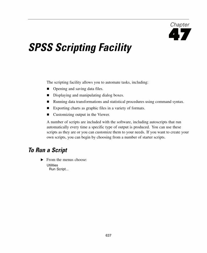
Chapter

47SPSS Scripting Facility

The scripting facility allows you to automate tasks, including:

Opening and saving data files.

Displaying and manipulating dialog boxes.

Running data transformations and statistical procedures using command syntax.

Exporting charts as graphic files in a variety of formats.

Customizing output in the Viewer.

A number of scripts are included with the software, including autoscripts that runautomatically every time a specific type of output is produced. You can use thesescripts as they are or you can customize them to your needs. If you want to create yourown scripts, you can begin by choosing from a number of starter scripts.

To Run a ScriptE From the menus choose:

UtilitiesRun Script...

637

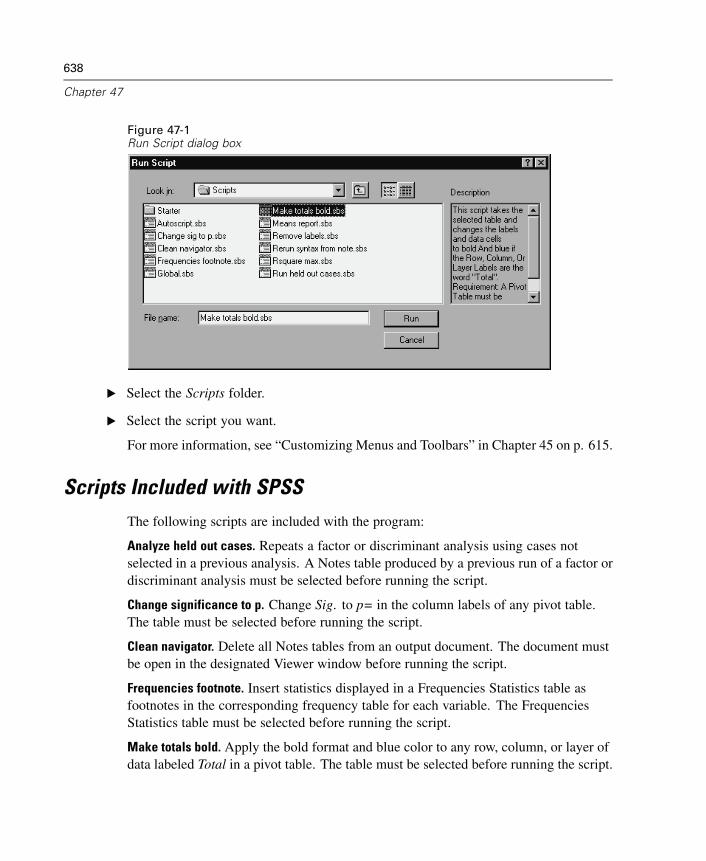
638

Chapter 47

Figure 47-1Run Script dialog box

E Select the Scripts folder.

E Select the script you want.

For more information, see “Customizing Menus and Toolbars” in Chapter 45 on p. 615.

Scripts Included with SPSSThe following scripts are included with the program:

Analyze held out cases. Repeats a factor or discriminant analysis using cases notselected in a previous analysis. A Notes table produced by a previous run of a factor ordiscriminant analysis must be selected before running the script.

Change significance to p. Change Sig. to p= in the column labels of any pivot table.The table must be selected before running the script.

Clean navigator. Delete all Notes tables from an output document. The document mustbe open in the designated Viewer window before running the script.

Frequencies footnote. Insert statistics displayed in a Frequencies Statistics table asfootnotes in the corresponding frequency table for each variable. The FrequenciesStatistics table must be selected before running the script.

Make totals bold. Apply the bold format and blue color to any row, column, or layer ofdata labeled Total in a pivot table. The table must be selected before running the script.

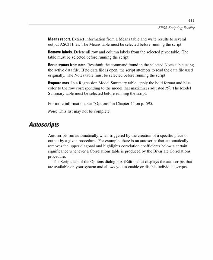
639

SPSS Scripting Facility

Means report. Extract information from a Means table and write results to severaloutput ASCII files. The Means table must be selected before running the script.

Remove labels. Delete all row and column labels from the selected pivot table. Thetable must be selected before running the script.

Rerun syntax from note. Resubmit the command found in the selected Notes table usingthe active data file. If no data file is open, the script attempts to read the data file usedoriginally. The Notes table must be selected before running the script.

Rsquare max. In a Regression Model Summary table, apply the bold format and bluecolor to the row corresponding to the model that maximizes adjusted R2. The ModelSummary table must be selected before running the script.

For more information, see “Options” in Chapter 44 on p. 595.

Note: This list may not be complete.

Autoscripts

Autoscripts run automatically when triggered by the creation of a specific piece ofoutput by a given procedure. For example, there is an autoscript that automaticallyremoves the upper diagonal and highlights correlation coefficients below a certainsignificance whenever a Correlations table is produced by the Bivariate Correlationsprocedure.

The Scripts tab of the Options dialog box (Edit menu) displays the autoscripts thatare available on your system and allows you to enable or disable individual scripts.

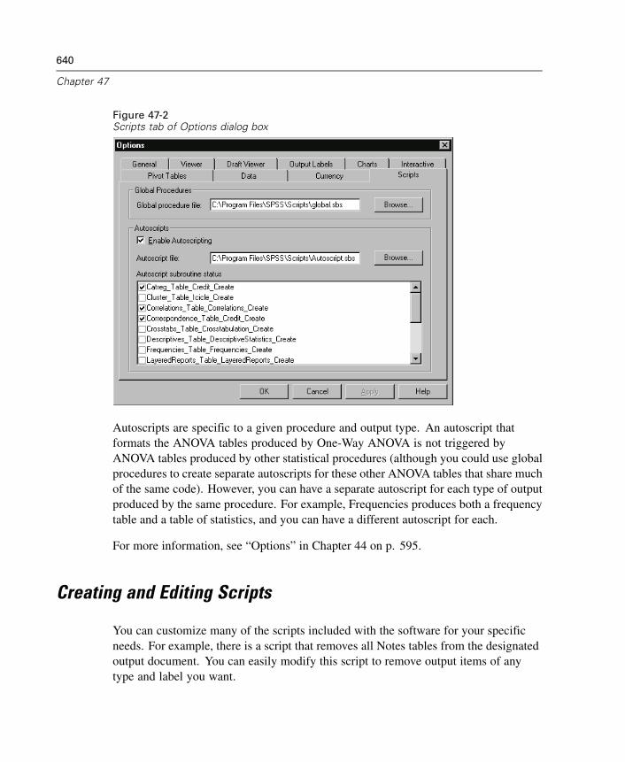
640

Chapter 47

Figure 47-2Scripts tab of Options dialog box

Autoscripts are specific to a given procedure and output type. An autoscript thatformats the ANOVA tables produced by One-Way ANOVA is not triggered byANOVA tables produced by other statistical procedures (although you could use globalprocedures to create separate autoscripts for these other ANOVA tables that share muchof the same code). However, you can have a separate autoscript for each type of outputproduced by the same procedure. For example, Frequencies produces both a frequencytable and a table of statistics, and you can have a different autoscript for each.

For more information, see “Options” in Chapter 44 on p. 595.

Creating and Editing Scripts

You can customize many of the scripts included with the software for your specificneeds. For example, there is a script that removes all Notes tables from the designatedoutput document. You can easily modify this script to remove output items of anytype and label you want.

641


Figure 47-3Modifying a script in the script window

If you prefer to create your own scripts, you can begin by choosing from a number ofstarter scripts.

To Edit a ScriptE From the menus choose:

FileOpen

Script...

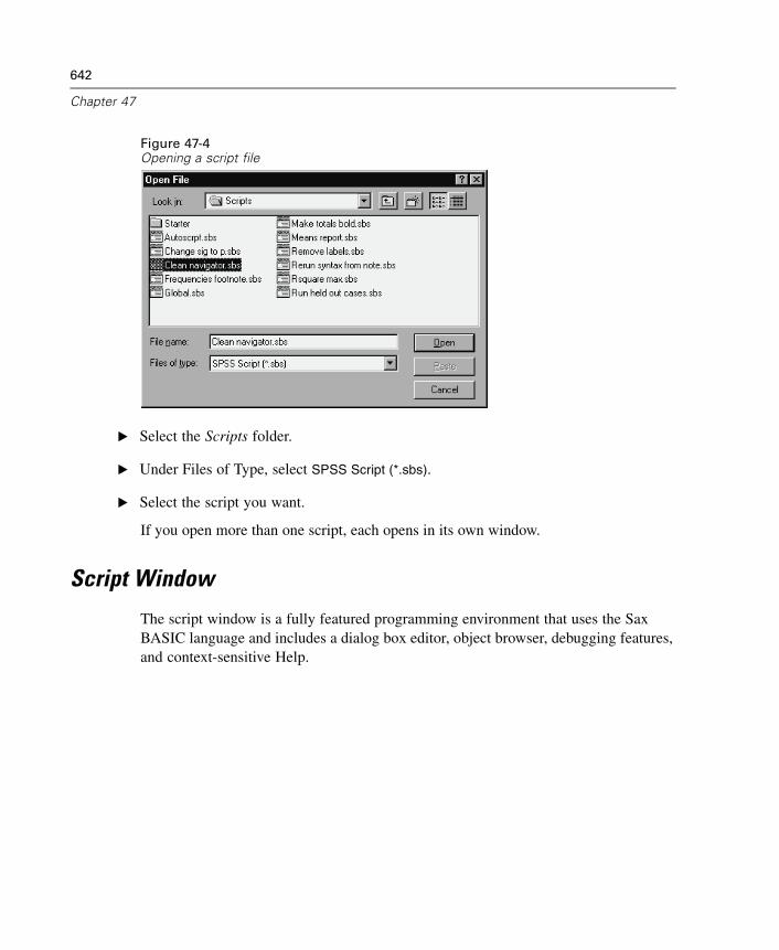
642

Chapter 47

Figure 47-4Opening a script file

E Select the Scripts folder.

E Under Files of Type, select SPSS Script (*.sbs).

E Select the script you want.

If you open more than one script, each opens in its own window.

Script Window

The script window is a fully featured programming environment that uses the SaxBASIC language and includes a dialog box editor, object browser, debugging features,and context-sensitive Help.

643


Figure 47-5Script window

As you move the cursor, the name of the current procedure is displayed at thetop of the window.

Terms colored blue are reserved words in BASIC (for example Sub, End Sub,and Dim). You can access context-sensitive Help on these terms by clicking themand pressing F1.

Terms colored magenta are objects, properties, or methods. You can also clickthese terms and press F1 for Help, but only where they appear in valid statementsand are colored magenta. (Clicking the name of an object in a comment will notwork because it brings up Help on the Sax BASIC language rather than on SPSSobjects.)

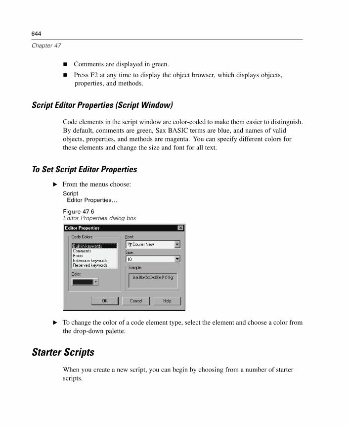
644

Chapter 47

Comments are displayed in green.

Press F2 at any time to display the object browser, which displays objects,properties, and methods.

Script Editor Properties (Script Window)

Code elements in the script window are color-coded to make them easier to distinguish.By default, comments are green, Sax BASIC terms are blue, and names of validobjects, properties, and methods are magenta. You can specify different colors forthese elements and change the size and font for all text.

To Set Script Editor Properties

E From the menus choose:Script

Editor Properties…

Figure 47-6Editor Properties dialog box

E To change the color of a code element type, select the element and choose a color fromthe drop-down palette.

Starter Scripts

When you create a new script, you can begin by choosing from a number of starterscripts.

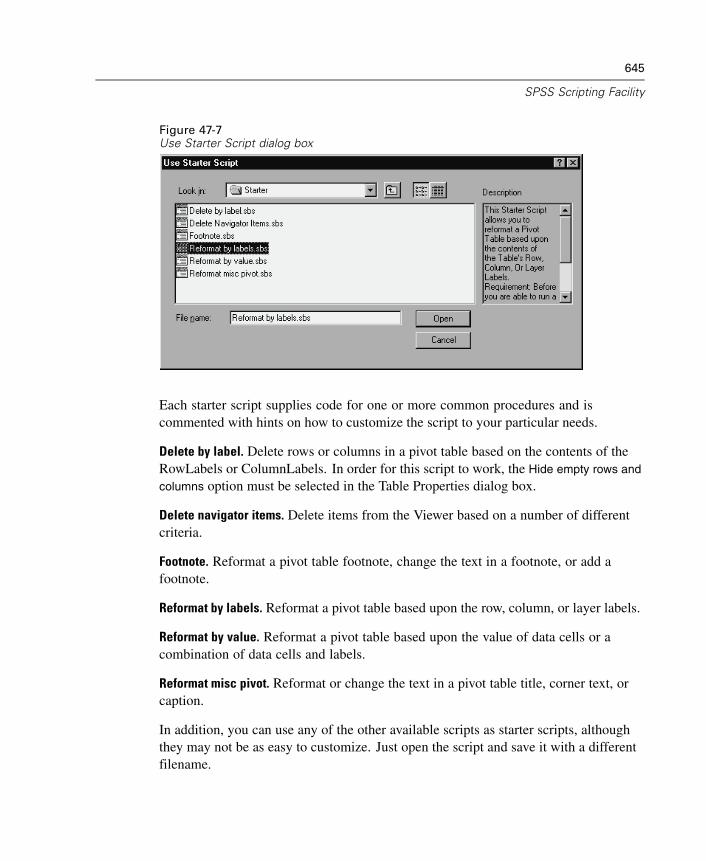
645


Figure 47-7Use Starter Script dialog box

Each starter script supplies code for one or more common procedures and iscommented with hints on how to customize the script to your particular needs.

Delete by label. Delete rows or columns in a pivot table based on the contents of theRowLabels or ColumnLabels. In order for this script to work, the Hide empty rows and

columns option must be selected in the Table Properties dialog box.

Delete navigator items. Delete items from the Viewer based on a number of differentcriteria.

Footnote. Reformat a pivot table footnote, change the text in a footnote, or add afootnote.

Reformat by labels. Reformat a pivot table based upon the row, column, or layer labels.

Reformat by value. Reformat a pivot table based upon the value of data cells or acombination of data cells and labels.

Reformat misc pivot. Reformat or change the text in a pivot table title, corner text, orcaption.

In addition, you can use any of the other available scripts as starter scripts, althoughthey may not be as easy to customize. Just open the script and save it with a differentfilename.

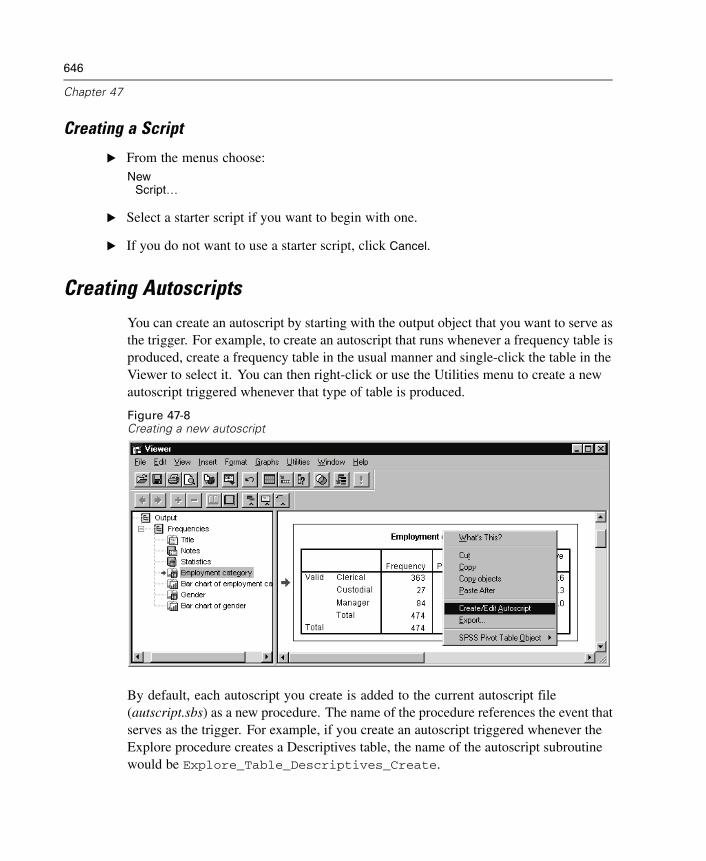
646

Chapter 47

Creating a Script

E From the menus choose:New

Script…

E Select a starter script if you want to begin with one.

E If you do not want to use a starter script, click Cancel.

Creating AutoscriptsYou can create an autoscript by starting with the output object that you want to serve asthe trigger. For example, to create an autoscript that runs whenever a frequency table isproduced, create a frequency table in the usual manner and single-click the table in theViewer to select it. You can then right-click or use the Utilities menu to create a newautoscript triggered whenever that type of table is produced.

Figure 47-8Creating a new autoscript

By default, each autoscript you create is added to the current autoscript file(autscript.sbs) as a new procedure. The name of the procedure references the event thatserves as the trigger. For example, if you create an autoscript triggered whenever theExplore procedure creates a Descriptives table, the name of the autoscript subroutinewould be Explore_Table_Descriptives_Create.

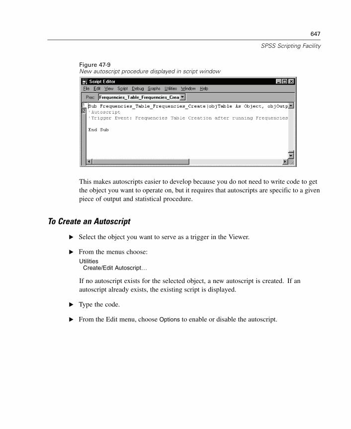
647


Figure 47-9New autoscript procedure displayed in script window

This makes autoscripts easier to develop because you do not need to write code to getthe object you want to operate on, but it requires that autoscripts are specific to a givenpiece of output and statistical procedure.

To Create an Autoscript

E Select the object you want to serve as a trigger in the Viewer.


Create/Edit Autoscript…

If no autoscript exists for the selected object, a new autoscript is created. If anautoscript already exists, the existing script is displayed.

E Type the code.

E From the Edit menu, choose Options to enable or disable the autoscript.

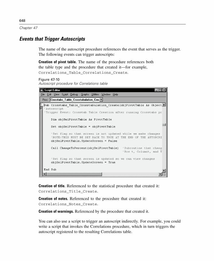
648

Chapter 47

Events that Trigger Autoscripts

The name of the autoscript procedure references the event that serves as the trigger.The following events can trigger autoscripts:

Creation of pivot table. The name of the procedure references boththe table type and the procedure that created it—for example,Correlations_Table_Correlations_Create.

Figure 47-10Autoscript procedure for Correlations table

Creation of title. Referenced to the statistical procedure that created it:Correlations_Title_Create.

Creation of notes. Referenced to the procedure that created it:Correlations_Notes_Create.

Creation of warnings. Referenced by the procedure that created it.

You can also use a script to trigger an autoscript indirectly. For example, you couldwrite a script that invokes the Correlations procedure, which in turn triggers theautoscript registered to the resulting Correlations table.

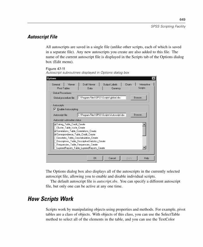
649


Autoscript File

All autoscripts are saved in a single file (unlike other scripts, each of which is savedin a separate file). Any new autoscripts you create are also added to this file. Thename of the current autoscript file is displayed in the Scripts tab of the Options dialogbox (Edit menu).

Figure 47-11Autoscript subroutines displayed in Options dialog box

The Options dialog box also displays all of the autoscripts in the currently selectedautoscript file, allowing you to enable and disable individual scripts.

The default autoscript file is autscript.sbs. You can specify a different autoscriptfile, but only one can be active at any one time.

How Scripts Work

Scripts work by manipulating objects using properties and methods. For example, pivottables are a class of objects. With objects of this class, you can use the SelectTablemethod to select all of the elements in the table, and you can use the TextColor

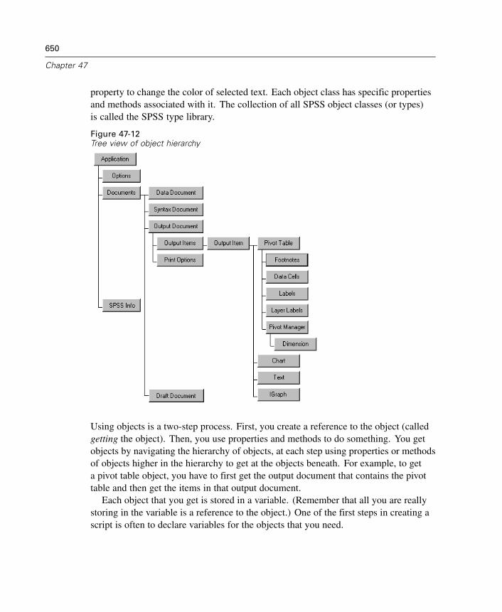
650

Chapter 47

property to change the color of selected text. Each object class has specific propertiesand methods associated with it. The collection of all SPSS object classes (or types)is called the SPSS type library.

Figure 47-12Tree view of object hierarchy

Using objects is a two-step process. First, you create a reference to the object (calledgetting the object). Then, you use properties and methods to do something. You getobjects by navigating the hierarchy of objects, at each step using properties or methodsof objects higher in the hierarchy to get at the objects beneath. For example, to geta pivot table object, you have to first get the output document that contains the pivottable and then get the items in that output document.

Each object that you get is stored in a variable. (Remember that all you are reallystoring in the variable is a reference to the object.) One of the first steps in creating ascript is often to declare variables for the objects that you need.

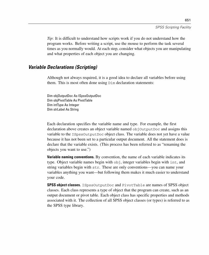
651


Tip: It is difficult to understand how scripts work if you do not understand how theprogram works. Before writing a script, use the mouse to perform the task severaltimes as you normally would. At each step, consider what objects you are manipulatingand what properties of each object you are changing.

Variable Declarations (Scripting)

Although not always required, it is a good idea to declare all variables before usingthem. This is most often done using Dim declaration statements:

Dim objOutputDoc As ISpssOutputDocDim objPivotTable As PivotTableDim intType As IntegerDim strLabel As String

Each declaration specifies the variable name and type. For example, the firstdeclaration above creates an object variable named objOutputDoc and assigns thisvariable to the ISpssOutputDoc object class. The variable does not yet have a valuebecause it has not been set to a particular output document. All the statement does isdeclare that the variable exists. (This process has been referred to as “renaming theobjects you want to use.”)

Variable naming conventions. By convention, the name of each variable indicates itstype. Object variable names begin with obj, integer variables begin with int, andstring variables begin with str. These are only conventions—you can name yourvariables anything you want—but following them makes it much easier to understandyour code.

SPSS object classes. ISpssOutputDoc and PivotTable are names of SPSS objectclasses. Each class represents a type of object that the program can create, such as anoutput document or pivot table. Each object class has specific properties and methodsassociated with it. The collection of all SPSS object classes (or types) is referred to asthe SPSS type library.

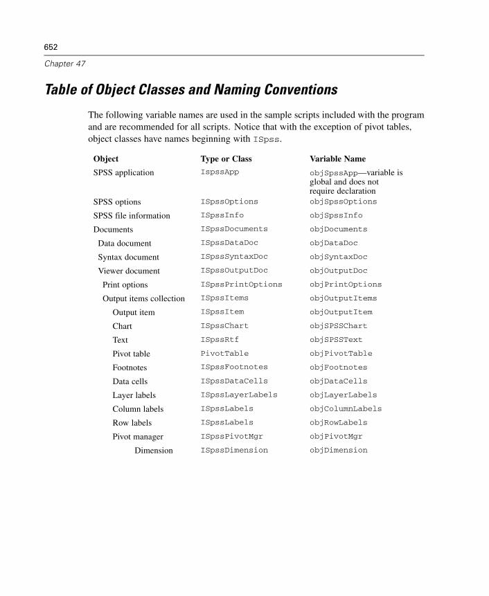
652

Chapter 47

Table of Object Classes and Naming Conventions

The following variable names are used in the sample scripts included with the programand are recommended for all scripts. Notice that with the exception of pivot tables,object classes have names beginning with ISpss.

Object Type or Class Variable Name

SPSS application IspssApp objSpssApp—variable isglobal and does notrequire declaration

SPSS options ISpssOptions objSpssOptions

SPSS file information ISpssInfo objSpssInfo

Documents ISpssDocuments objDocuments

Data document ISpssDataDoc objDataDoc

Syntax document ISpssSyntaxDoc objSyntaxDoc

Viewer document ISpssOutputDoc objOutputDoc

Print options ISpssPrintOptions objPrintOptions

Output items collection ISpssItems objOutputItems

Output item ISpssItem objOutputItem

Chart ISpssChart objSPSSChart

Text ISpssRtf objSPSSText

Pivot table PivotTable objPivotTable

Footnotes ISpssFootnotes objFootnotes

Data cells ISpssDataCells objDataCells

Layer labels ISpssLayerLabels objLayerLabels

Column labels ISpssLabels objColumnLabels

Row labels ISpssLabels objRowLabels

Pivot manager ISpssPivotMgr objPivotMgr

Dimension ISpssDimension objDimension

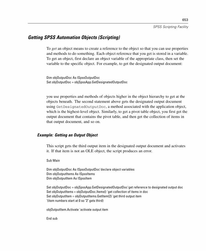
653


Getting SPSS Automation Objects (Scripting)

To get an object means to create a reference to the object so that you can use propertiesand methods to do something. Each object reference that you get is stored in a variable.To get an object, first declare an object variable of the appropriate class, then set thevariable to the specific object. For example, to get the designated output document:

Dim objOutputDoc As ISpssOutputDocSet objOutputDoc = objSpssApp.GetDesignatedOutputDoc

you use properties and methods of objects higher in the object hierarchy to get at theobjects beneath. The second statement above gets the designated output documentusing GetDesignatedOutputDoc, a method associated with the application object,which is the highest-level object. Similarly, to get a pivot table object, you first get theoutput document that contains the pivot table, and then get the collection of items inthat output document, and so on.

Example: Getting an Output Object

This script gets the third output item in the designated output document and activatesit. If that item is not an OLE object, the script produces an error.

Sub Main

Dim objOutputDoc As ISpssOutputDoc'declare object variablesDim objOutputItems As ISpssItemsDim objOutputItem As ISpssItem

Set objOutputDoc = objSpssApp.GetDesignatedOutputDoc'get reference to designated output docSet objOutputItems = objOutputDoc.Items() 'get collection of items in docSet objOutputItem = objOutputItems.GetItem(2) 'get third output item'(item numbers start at 0 so "2" gets third)

objOutputItem.Activate 'activate output item

End sub

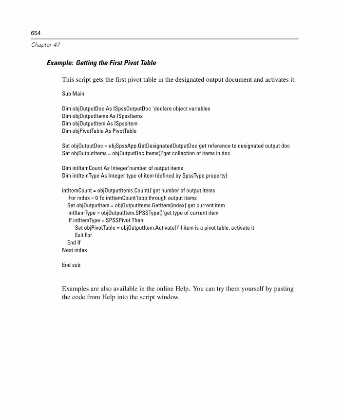
654

Chapter 47

Example: Getting the First Pivot Table

This script gets the first pivot table in the designated output document and activates it.

Sub Main

Dim objOutputDoc As ISpssOutputDoc 'declare object variablesDim objOutputItems As ISpssItemsDim objOutputItem As ISpssItemDim objPivotTable As PivotTable

Set objOutputDoc = objSpssApp.GetDesignatedOutputDoc'get reference to designated output docSet objOutputItems = objOutputDoc.Items()'get collection of items in doc

Dim intItemCount As Integer'number of output itemsDim intItemType As Integer'type of item (defined by SpssType property)

intItemCount = objOutputItems.Count()'get number of output itemsFor index = 0 To intItemCount'loop through output itemsSet objOutputItem = objOutputItems.GetItem(index)'get current itemintItemType = objOutputItem.SPSSType()'get type of current itemIf intItemType = SPSSPivot Then

Set objPivotTable = objOutputItem.Activate()'if item is a pivot table, activate itExit For

End IfNext index

End sub

Examples are also available in the online Help. You can try them yourself by pastingthe code from Help into the script window.

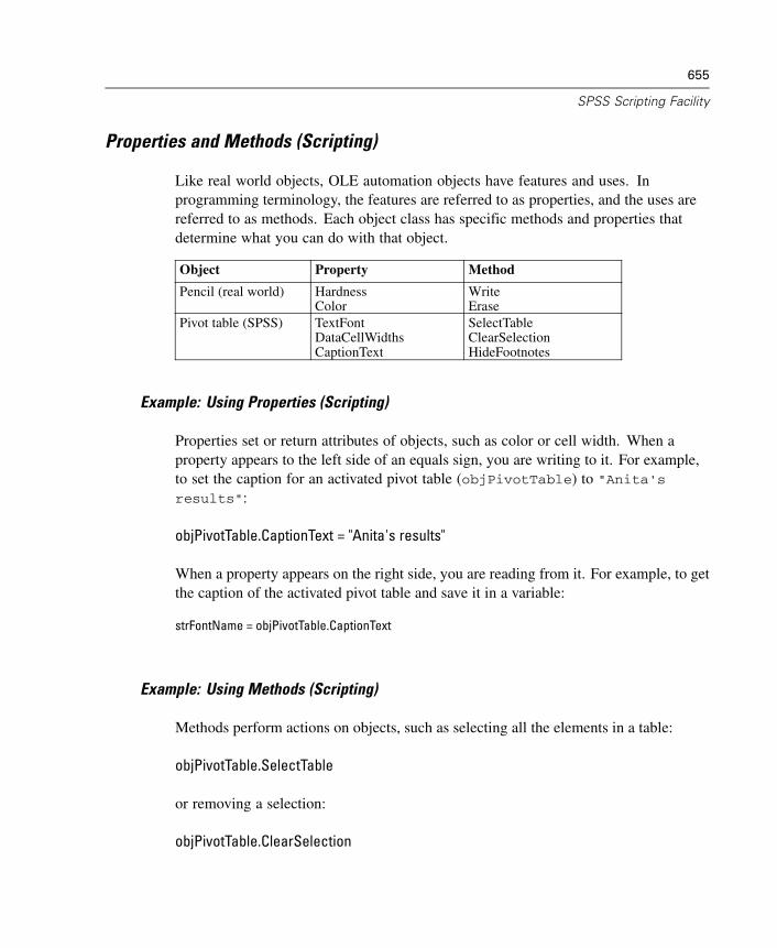
655


Properties and Methods (Scripting)

Like real world objects, OLE automation objects have features and uses. Inprogramming terminology, the features are referred to as properties, and the uses arereferred to as methods. Each object class has specific methods and properties thatdetermine what you can do with that object.

Object Property Method

Pencil (real world) HardnessColor

WriteErase

Pivot table (SPSS) TextFontDataCellWidthsCaptionText

SelectTableClearSelectionHideFootnotes

Example: Using Properties (Scripting)

Properties set or return attributes of objects, such as color or cell width. When aproperty appears to the left side of an equals sign, you are writing to it. For example,to set the caption for an activated pivot table (objPivotTable) to "Anita's

results":

objPivotTable.CaptionText = "Anita's results"

When a property appears on the right side, you are reading from it. For example, to getthe caption of the activated pivot table and save it in a variable:

strFontName = objPivotTable.CaptionText

Example: Using Methods (Scripting)

Methods perform actions on objects, such as selecting all the elements in a table:

objPivotTable.SelectTable

or removing a selection:

objPivotTable.ClearSelection

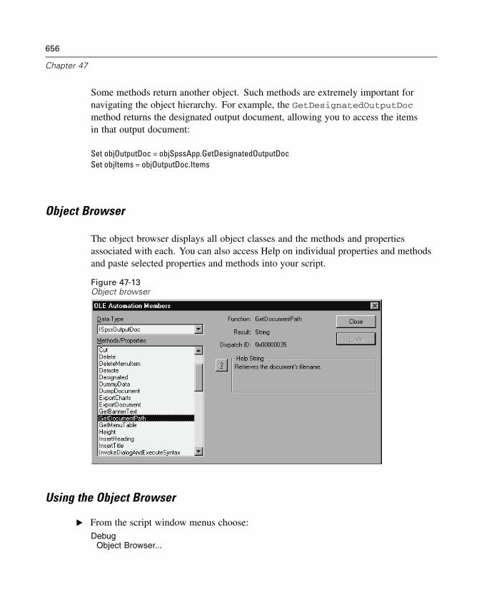
656

Chapter 47

Some methods return another object. Such methods are extremely important fornavigating the object hierarchy. For example, the GetDesignatedOutputDocmethod returns the designated output document, allowing you to access the itemsin that output document:

Set objOutputDoc = objSpssApp.GetDesignatedOutputDocSet objItems = objOutputDoc.Items

Object Browser

The object browser displays all object classes and the methods and propertiesassociated with each. You can also access Help on individual properties and methodsand paste selected properties and methods into your script.

Figure 47-13Object browser

Using the Object Browser

E From the script window menus choose:Debug

Object Browser...

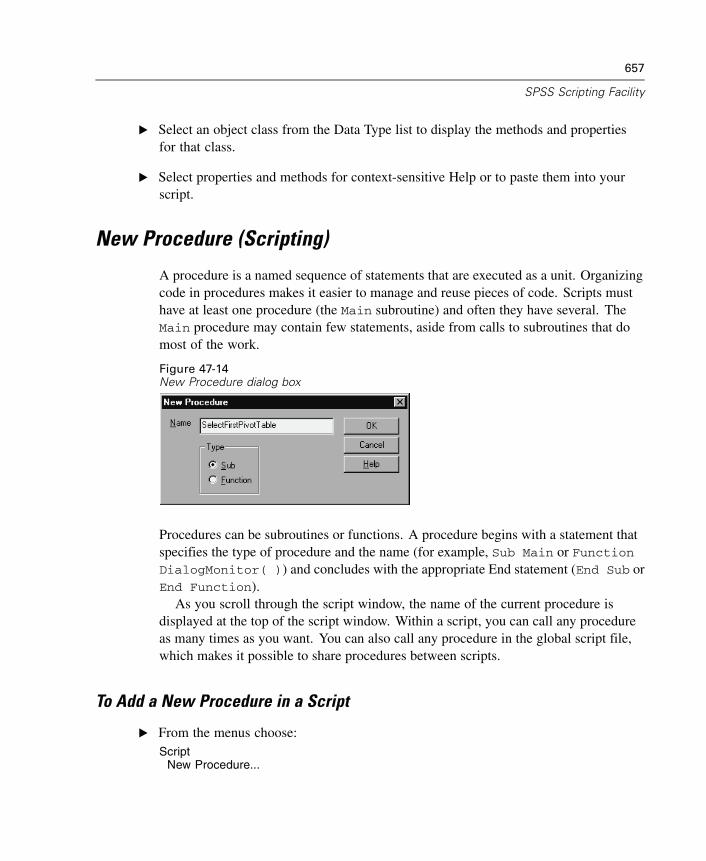
657


E Select an object class from the Data Type list to display the methods and propertiesfor that class.

E Select properties and methods for context-sensitive Help or to paste them into yourscript.

New Procedure (Scripting)

A procedure is a named sequence of statements that are executed as a unit. Organizingcode in procedures makes it easier to manage and reuse pieces of code. Scripts musthave at least one procedure (the Main subroutine) and often they have several. TheMain procedure may contain few statements, aside from calls to subroutines that domost of the work.

Figure 47-14New Procedure dialog box

Procedures can be subroutines or functions. A procedure begins with a statement thatspecifies the type of procedure and the name (for example, Sub Main or FunctionDialogMonitor( )) and concludes with the appropriate End statement (End Sub orEnd Function).

As you scroll through the script window, the name of the current procedure isdisplayed at the top of the script window. Within a script, you can call any procedureas many times as you want. You can also call any procedure in the global script file,which makes it possible to share procedures between scripts.

To Add a New Procedure in a Script


New Procedure...

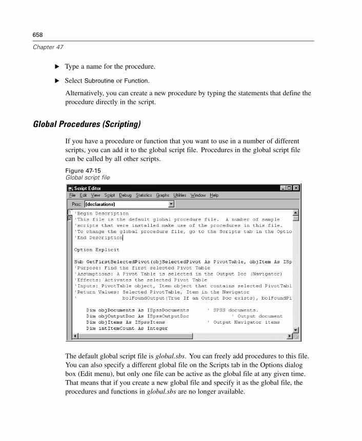
658

Chapter 47

E Type a name for the procedure.

E Select Subroutine or Function.

Alternatively, you can create a new procedure by typing the statements that define theprocedure directly in the script.

Global Procedures (Scripting)

If you have a procedure or function that you want to use in a number of differentscripts, you can add it to the global script file. Procedures in the global script filecan be called by all other scripts.

Figure 47-15Global script file

The default global script file is global.sbs. You can freely add procedures to this file.You can also specify a different global file on the Scripts tab in the Options dialogbox (Edit menu), but only one file can be active as the global file at any given time.That means that if you create a new global file and specify it as the global file, theprocedures and functions in global.sbs are no longer available.

659


You can view the global script file in any script window (click the #2 tab on the leftside of the window just below the toolbar), but you can edit it in only one windowat a time.

Global procedures must be called by other script procedures. You cannot run aglobal script directly from the Utilities menu or a script window.

Adding a Description to a Script

You can add a description to be displayed in the Run Script and Use Starter Scriptdialog boxes. Just add a comment on the first line of the script that starts with Begin

Description, followed by the desired comment (one or more lines), followed byEnd Description. For example:

'Begin Description'This script changes "Sig." to "p=" in the column labels of any pivot table.'Requirement: The Pivot Table that you want to change must be selected.'End Description

The description must be formatted as a comment (each line beginning with anapostrophe).

Scripting Custom Dialog Boxes

There are two steps to implementing a custom dialog box: first create the dialog boxusing the UserDialog Editor, and then create a dialog monitor function (DialogFunc)that monitors the dialog box and defines its behavior.

The dialog box itself is defined by a Begin Dialog...End Dialog block.You do not need to type this code directly—the UserDialog Editor provides an easy,graphical way to define the dialog box.

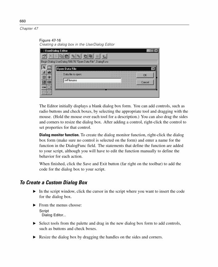
660

Chapter 47

Figure 47-16Creating a dialog box in the UserDialog Editor

The Editor initially displays a blank dialog box form. You can add controls, such asradio buttons and check boxes, by selecting the appropriate tool and dragging with themouse. (Hold the mouse over each tool for a description.) You can also drag the sidesand corners to resize the dialog box. After adding a control, right-click the control toset properties for that control.

Dialog monitor function. To create the dialog monitor function, right-click the dialogbox form (make sure no control is selected on the form) and enter a name for thefunction in the DialogFunc field. The statements that define the function are addedto your script, although you will have to edit the function manually to define thebehavior for each action.

When finished, click the Save and Exit button (far right on the toolbar) to add thecode for the dialog box to your script.

To Create a Custom Dialog Box

E In the script window, click the cursor in the script where you want to insert the codefor the dialog box.


Dialog Editor...

E Select tools from the palette and drag in the new dialog box form to add controls,such as buttons and check boxes.

E Resize the dialog box by dragging the handles on the sides and corners.

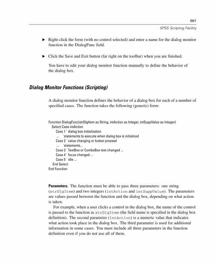
661


E Right-click the form (with no control selected) and enter a name for the dialog monitorfunction in the DialogFunc field.

E Click the Save and Exit button (far right on the toolbar) when you are finished.

You have to edit your dialog monitor function manually to define the behavior ofthe dialog box.

Dialog Monitor Functions (Scripting)

A dialog monitor function defines the behavior of a dialog box for each of a number ofspecified cases. The function takes the following (generic) form:

Function DialogFunc(strDlgItem as String, intAction as Integer, intSuppValue as Integer)Select Case intAction

Case 1 ' dialog box initialization... 'statements to execute when dialog box is initializedCase 2 ' value changing or button pressed... 'statements...Case 3 ' TextBox or ComboBox text changed ...Case 4 ' focus changed ...Case 5 ' idle ...

End SelectEnd Function

Parameters. The function must be able to pass three parameters: one string(strDlgItem) and two integers (intAction and intSuppValue). The parametersare values passed between the function and the dialog box, depending on what actionis taken.

For example, when a user clicks a control in the dialog box, the name of the controlis passed to the function as strDlgItem (the field name is specified in the dialog boxdefinition). The second parameter (intAction) is a numeric value that indicateswhat action took place in the dialog box. The third parameter is used for additionalinformation in some cases. You must include all three parameters in the functiondefinition even if you do not use all of them.

662

Chapter 47

Select Case intAction. The value of intAction indicates what action took place in thedialog box. For example, when the dialog box initializes, intAction = 1. If the userpresses a button, intAction changes to 2, and so on. There are five possible actions,and you can specify statements that execute for each action as indicated below. You donot need to specify all five possible cases—only the ones that apply. For example, ifyou do not want any statements to execute on initialization, omit Case 1.

Case intAction = 1. Specify statements to execute when the dialog box is initialized.For example, you could disable one or more controls or add a beep. The stringstrDlgItem is a null string; intSuppValue is 0.

Case 2. Executes when a button is pushed or when a value changes in a CheckBox,DropListBox, ListBox, or OptionGroup control. If a button is pushed,strDlgItem is the button, intSuppValue is meaningless, and you must setDialogFunc = True to prevent the dialog box from closing. If a value changes,strDlgItem is the item whose value has changed, and intSuppValue is thenew value.

Case 3. Executes when a value changes in a TextBox or ComboBox control.The string strDlgItem is the control whose text changed and is losing focus;intSuppValue is the number of characters.

Case 4. Executes when the focus changes in the dialog box. The stringstrDlgItem is gaining focus, and intSuppValue is the item that is losing focus(the first item is 0, second is 1, and so on).

Case 5. Idle processing. The string strDlgItem is a null string; intSuppValueis 0. Set DialogFunc = True to continue receiving idle actions.

For more information, see the examples and the DialogFunc prototype in the SaxBASIC Language Reference Help file.

Example: Scripting a Simple Dialog Box

This script creates a simple dialog box that opens a data file. See related sections forexplanations of the BuildDialog subroutine and dialog monitor function.

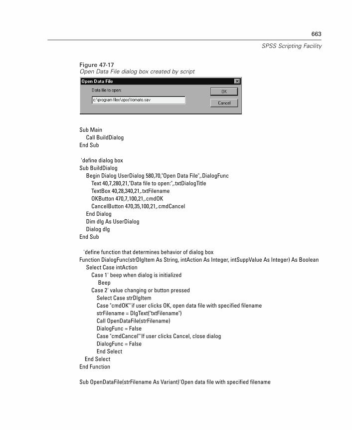
663


Figure 47-17Open Data File dialog box created by script

Sub MainCall BuildDialog

End Sub

'define dialog boxSub BuildDialog

Begin Dialog UserDialog 580,70,"Open Data File",.DialogFuncText 40,7,280,21,"Data file to open:",.txtDialogTitleTextBox 40,28,340,21,.txtFilenameOKButton 470,7,100,21,.cmdOKCancelButton 470,35,100,21,.cmdCancel

End DialogDim dlg As UserDialogDialog dlg

End Sub

'define function that determines behavior of dialog boxFunction DialogFunc(strDlgItem As String, intAction As Integer, intSuppValue As Integer) As Boolean

Select Case intActionCase 1' beep when dialog is initialized

BeepCase 2' value changing or button pressed

Select Case strDlgItemCase "cmdOK"'if user clicks OK, open data file with specified filenamestrFilename = DlgText("txtFilename")Call OpenDataFile(strFilename)DialogFunc = FalseCase "cmdCancel"'If user clicks Cancel, close dialogDialogFunc = FalseEnd Select

End SelectEnd Function

Sub OpenDataFile(strFilename As Variant)'Open data file with specified filename

664

Chapter 47

Dim objDataDoc As ISpssDataDocSet objDataDoc = objSpssApp.OpenDataDoc(strFilename)

End Sub

Examples are also available in the online Help. You can try them yourself by pastingthe code from Help into the script window.

Debugging Scripts

The Debug menu allows you to step through your code, executing one line orsubroutine at a time and viewing the result. You can also insert a break point in thescript to pause the execution at the line that contains the break point.

To debug an autoscript, open the autoscript file in a script window, insert breakpoints in the procedure that you want to debug, and then run the statistical procedurethat triggers the autoscript.

Step Into. Execute the current line. If the current line is a subroutine or function call,stop on the first line of that subroutine or function.

Step Over. Execute to the next line. If the current line is a subroutine or function call,execute the subroutine or function completely.

Step Out. Step out of the current subroutine or function call.

Step to Cursor. Execute to the current line.

Toggle Break. Insert or remove a break point. The script pauses at the break point, andthe debugging pane is displayed.

Quick Watch. Display the value of the current expression.

Add Watch. Add the current expression to the watch window.

Object Browser. Display the object browser.

Set Next Statement. Set the next statement to be executed. Only statements in thecurrent subroutine/function can be selected.

Show Next Statement. Display the next statement to be executed.

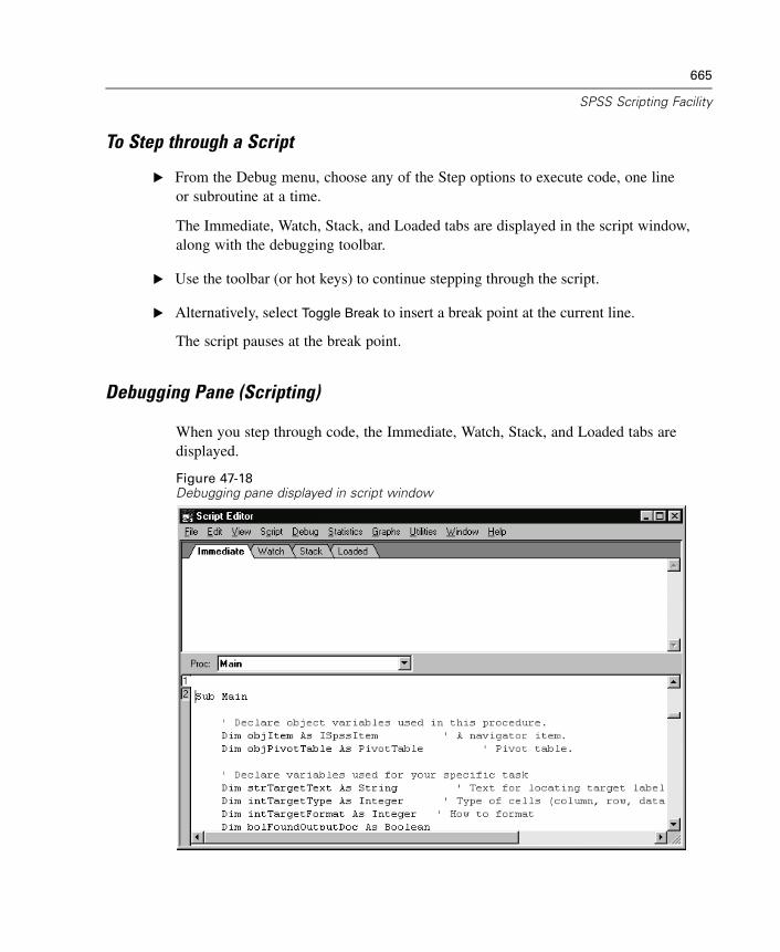
665


To Step through a Script

E From the Debug menu, choose any of the Step options to execute code, one lineor subroutine at a time.

The Immediate, Watch, Stack, and Loaded tabs are displayed in the script window,along with the debugging toolbar.

E Use the toolbar (or hot keys) to continue stepping through the script.

E Alternatively, select Toggle Break to insert a break point at the current line.

The script pauses at the break point.

Debugging Pane (Scripting)

When you step through code, the Immediate, Watch, Stack, and Loaded tabs aredisplayed.

Figure 47-18Debugging pane displayed in script window

666

Chapter 47

Immediate tab. Click the name of any variable and click the eyeglass button to displaythe current value of the variable. You can also evaluate an expression, assign a variable,or call a subroutine.

Type ?expr and press Enter to show the value of expr.

Type var = expr and press Enter to change the value of var.

Type subname args and press Enter to call a subroutine or built-in instruction.

Type Trace and press Enter to toggle trace mode. Trace mode prints each statementin the immediate window when a script is running.

Watch tab. To display a variable, function, or expression, click it and choose Add Watch

from the Debug menu. Displayed values are updated each time execution pauses.You can edit the expression to the left of ->. Press Enter to update all the valuesimmediately. Press Ctrl-Y to delete the line.

Stack tab. Displays the lines that called the current statement. The first line is thecurrent statement, the second line is the one that called the first, and so on. Click anyline to highlight that line in the edit window.

Loaded tab. List the currently active scripts. Click a line to view that script.

Script Files and Syntax Files

Syntax files (*.sps) are not the same as script files (*.sbs). Syntax files have commandswritten in the command language that allows you to run statistical procedures and datatransformations. While scripts allow you to manipulate output and automate othertasks that you normally perform using the graphical interface of menus and dialogboxes, the command language provides an alternative method for communicatingdirectly with the program’s back end, the part of the system that handles statisticalcomputations and data transformations.

You can combine scripts and syntax files for even greater flexibility, by running ascript from within command syntax, or by embedding command syntax within a script.

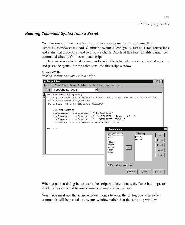
667


Running Command Syntax from a Script

You can run command syntax from within an automation script using theExecuteCommands method. Command syntax allows you to run data transformationsand statistical procedures and to produce charts. Much of this functionality cannot beautomated directly from command scripts.

The easiest way to build a command syntax file is to make selections in dialog boxesand paste the syntax for the selections into the script window.

Figure 47-19Pasting command syntax into a script

When you open dialog boxes using the script window menus, the Paste button pastesall of the code needed to run commands from within a script.

Note: You must use the script window menus to open the dialog box; otherwise,commands will be pasted to a syntax window rather than the scripting window.

668

Chapter 47

Pasting SPSS Command Syntax into a Script

E From the script window menus, choose commands from the Statistics, Graphs, andUtilities menus to open dialog boxes.

E Make selections in the dialog box.

E Click Paste.

Note: You must use the script window menus to open the dialog box; otherwise,commands will be pasted to a syntax window rather than the scripting window.

Running a Script from Command Syntax

You can use the SCRIPT command to run a script from within command syntax.Specify the name of the script you want to run, with the filename enclosed in quotes, asfollows:

SCRIPT 'C:\PROGRAM FILES\SPSS\CLEAN NAVIGATOR.SBS'.


Chapter

48Output Management System

The Output Management System (OMS) provides the ability to automatically writeselected categories of output to different output files in different formats. Formatsinclude:

SPSS data file format (.sav). Output that would be displayed in pivot tables in theViewer can be written out in the form of an SPSS data file, making it possible touse output as input for subsequent commands.

XML. Tables, text output, and even many charts can be written out in XML format.

HTML. Tables and text output can be written out in HTML format. Standard (notinteractive) charts and tree model diagrams (Classification Tree option) can beincluded as image files. The image files are saved in a separate subdirectory(folder).

Text. Tables and text output can be written out as tab-delimited or space-separatedtext.

To Use the Output Management System Control Panel


OMS Control Panel...

669

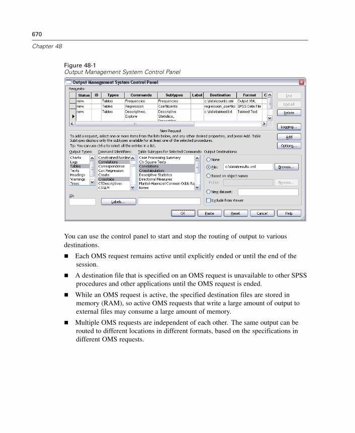
670

Chapter 48

Figure 48-1Output Management System Control Panel

You can use the control panel to start and stop the routing of output to variousdestinations.

Each OMS request remains active until explicitly ended or until the end of thesession.

A destination file that is specified on an OMS request is unavailable to other SPSSprocedures and other applications until the OMS request is ended.

While an OMS request is active, the specified destination files are stored inmemory (RAM), so active OMS requests that write a large amount of output toexternal files may consume a large amount of memory.

Multiple OMS requests are independent of each other. The same output can berouted to different locations in different formats, based on the specifications indifferent OMS requests.

671

Output Management System

The order of the output objects in any particular destination is the order inwhich they were created, which is determined by the order and operation of theprocedures that generate the output.

OMS cannot route charts or warnings objects created by interactive graphicsprocedures (Graphs menu, Interactive submenu) or maps created by the mappingprocedures (Graphs menu, Map submenu).

To Add New OMS Requests

E Select the output types (tables, charts, and so on) that you want to include. (For moreinformation, see “Output Object Types” on p. 673.)

E Select the commands to include. If you want to include all output, select all items in thelist. (For more information, see “Command Identifiers and Table Subtypes” on p. 675.)

E For commands that produce pivot table output, select the specific table types to include.

The list displays only the tables that are available in the selected commands; any tabletype that is available in one or more of the selected commands is displayed in the list.If no commands are selected, all table types are displayed. (For more information, see“Command Identifiers and Table Subtypes” on p. 675.)

E To select tables based on text labels instead of subtypes, click Labels. (For moreinformation, see “Labels” on p. 676.)

E Click Options to specify the output format (for example, SPSS data file, XML, orHTML). (By default, Output XML format is used. For more information, see “OMSOptions” on p. 677.)

E Specify an output destination:

File. All selected output is routed to a single file.

Based on object names. Output is routed to multiple destination files based on objectnames. A separate file is created for each output object, with a filename based oneither table subtype names or table labels. Enter the destination folder name.

New dataset. For SPSS data file format output, you can route the output to adataset. The dataset is available for subsequent use in the same session but is notsaved unless you explicitly save it as a file prior to the end of the session. Thisoption is available only for SPSS data file format output. Dataset names mustconform to SPSS variable-naming rules. For more information, see “VariableNames” in Chapter 5 on p. 88.

672

Chapter 48

E Optionally:

Exclude the selected output from the Viewer. If you select Exclude from Viewer,the output types in the OMS request will not be displayed in the Viewer window.If multiple active OMS requests include the same output types, the display ofthose output types in the Viewer is determined by the most recent OMS requestthat contains those output types. For more information, see “Excluding OutputDisplay from the Viewer” on p. 683.

Assign an ID string to the request. All requests are automatically assigned an IDvalue, and you can override the system default ID string with a descriptive ID,which can be useful if you have multiple active requests that you want to identifyeasily. ID values that you assign cannot start with a dollar sign ($).

The following tips are for selecting multiple items in a list:

Press Ctrl-A to select all items in a list.

Use Shift-click to select multiple contiguous items.

Use Ctrl-click to select multiple noncontiguous items.

To End and Delete OMS Requests

Active and new OMS requests are displayed in the Requests list, with the mostrecent request at the top. You can change the widths of the information columns byclicking and dragging the borders, and you can scroll the list horizontally to see moreinformation about a particular request.

An asterisk (*) after the word Active in the Status column indicates an OMS requestthat was created with command syntax that includes features that are not available inthe Control Panel.

To end a specific, active OMS request:

E In the Requests list, click any cell in the row for the request.

E Click End.

To end all active OMS requests:

E Click End All.

To delete a new request (a request that has been added but is not yet active):

E In the Requests list, click any cell in the row for the request.

673


E Click Delete.

Note: Active OMS requests are not ended until you click OK.

Output Object Types

There are seven different types of output objects:

Charts. Charts (except “interactive” charts and maps). Chart objects are included onlywith XML and HTML destination formats. For HTML format, the chart image filesare saved in a separate subdirectory (folder).

Logs. Log text objects. Log objects contain certain types of error and warningmessages. Depending on your Options settings (Edit menu, Options, Viewer tab), logobjects may also contain the command syntax that is executed during the session. Logobjects are labeled Log in the outline pane of the Viewer.

Tables. Output objects that are pivot tables in the Viewer (includes Notes tables).Tables are the only output objects that can be routed to SPSS data file (.sav) format.

Text. Text objects that aren’t logs or headings (includes objects labeled Text Output inthe outline pane of the Viewer).

Trees. Tree model diagrams that are produced by the Classification Tree option. Treeobjects are included only with XML and HTML destination formats.

Headings. Text objects that are labeled Title in the outline pane of the Viewer. ForOutput XML format, heading text objects are not included.

Warnings. Warnings objects. Warnings objects contain certain types of error andwarning messages.

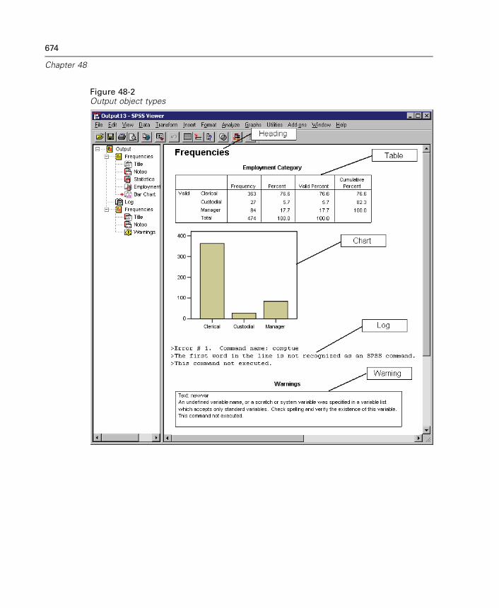
674

Chapter 48

Figure 48-2Output object types

675


Command Identifiers and Table Subtypes

Command Identifiers

Command identifiers are available for all statistical and charting procedures and anyother commands that produce blocks of output with their own identifiable heading inthe outline pane of the Viewer. These identifiers are usually (but not always) the sameor similar to the procedure names on the menus and dialog box titles, which are usually(but not always) similar to the underlying SPSS command names. For example, thecommand identifier for the Frequencies procedure is “Frequencies,” and the underlyingcommand name is also the same.

There are, however, some cases where the procedure name and the commandidentifier and/or the command name are not all that similar. For example, all of theprocedures on the Nonparametric Tests submenu (from the Analyze menu) use thesame underlying command, and the command identifier is the same as the underlyingcommand name: Npar Tests.

Table Subtypes

Table subtypes are the different types of pivot tables that can be produced. Somesubtypes are produced by only one command; other subtypes can be produced bymultiple commands (although the tables may not look similar). Although table subtypenames are generally descriptive, there can be many names to choose from (particularlyif you have selected a large number of commands); also, two subtypes may have verysimilar names.

To Find Command Identifiers and Table Subtypes

When in doubt, you can find command identifiers and table subtype names in theViewer window:

E Run the procedure to generate some output in the Viewer.

E Right-click the item in the outline pane of the Viewer.

E Choose Copy OMS Command Identifier or Copy OMS Table Subtype.

E Paste the copied command identifier or table subtype name into any text editor (such asan SPSS syntax window).

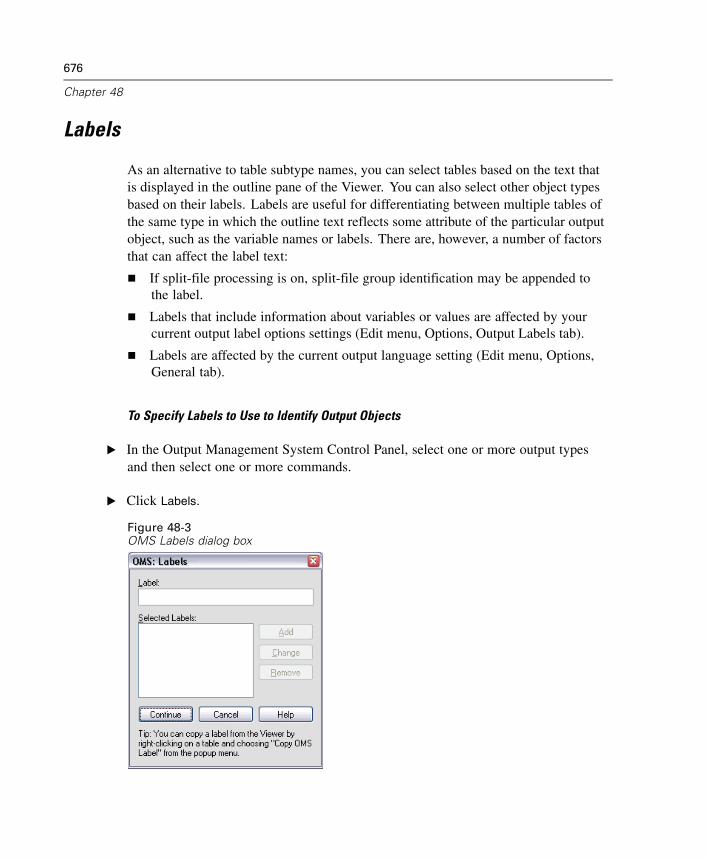
676

Chapter 48

Labels

As an alternative to table subtype names, you can select tables based on the text thatis displayed in the outline pane of the Viewer. You can also select other object typesbased on their labels. Labels are useful for differentiating between multiple tables ofthe same type in which the outline text reflects some attribute of the particular outputobject, such as the variable names or labels. There are, however, a number of factorsthat can affect the label text:

If split-file processing is on, split-file group identification may be appended tothe label.

Labels that include information about variables or values are affected by yourcurrent output label options settings (Edit menu, Options, Output Labels tab).

Labels are affected by the current output language setting (Edit menu, Options,General tab).

To Specify Labels to Use to Identify Output Objects

E In the Output Management System Control Panel, select one or more output typesand then select one or more commands.

E Click Labels.

Figure 48-3OMS Labels dialog box

677


E Enter the label exactly as it appears in the outline pane of the Viewer window. (You canalso right-click the item in the outline, choose Copy OMS Label, and paste the copiedlabel into the Label text field.)

E Click Add.

E Repeat the process for each label that you want to include.

E Click Continue.

Wildcards

You can use an asterisk (*) as the last character of the label string as a wildcardcharacter. All labels that begin with the specified string (except for the asterisk) willbe selected. This process works only when the asterisk is the last character, becauseasterisks can appear as valid characters inside a label.

OMS Options

You can use the OMS Options dialog box to:

Specify the output format.

Include or exclude chart and tree model diagram output and specify the graphicformat.

Specify what table dimension elements should go into the row dimension.

For SPSS data file format, include a variable that identifies the sequential tablenumber that is the source for each case.

To Specify OMS Options

E Click Options in the Output Management System Control Panel.

678

Chapter 48

Figure 48-4OMS Options dialog box

Format

Output XML. XML that conforms to the spss-output schema. Standard charts areincluded as XML that conforms to the vizml schema. You can also export all charts andmaps as separate files in the selected graphics format.

HTML. Output objects that would be pivot tables in the Viewer are converted to simpleHTML tables. No TableLook attributes (font characteristics, border styles, colors, andso on) are supported. Text output objects are tagged <PRE> in the HTML. If youchoose to include charts, they are exported as separate files in the selected graphicsformat and are embedded by reference (<IMG SRC='filename.ext'>) in the HTMLdocument. The image files are saved in a separate subdirectory (folder).

SPSS Data File. This format is a binary file format. All output object types other thantables are excluded. Each column of a table becomes a variable in the data file. Touse a data file that is created with OMS in the same session, you must end the activeOMS request before you can open the data file. For more information, see “RoutingOutput to SPSS Data Files” on p. 683.

679


SVWS XML. XML used by SmartViewer Web Server. This is actually a JAR/ZIPfile containing XML, CSV, and other files. SmartViewer Web Server is a separate,server-based product.

Text. Space-separated text. Output is written as text, with tabular output aligned withspaces for fixed-pitch fonts. All charts and maps are excluded.

Tabbed Text. Tab-delimited text. For output that is displayed as pivot tables in theViewer, tabs delimit table column elements. Text block lines are written as is; noattempt is made to divide them with tabs at useful places. All charts and maps areexcluded.

Graphics Images

For HTML format, you can include charts (excluding interactive charts) and tree modeldiagrams as image files. A separate image file is created for each chart and/or tree, andstandard <IMG SRC='filename'> tags are included in the HTML for each image file.

Image files are saved in a separate subdirectory (folder). The subdirectory name isthe name of the HTML destination file, without any extension and with _files appendedto the end. For example, if the HTML destination file is julydata.htm, the imagessubdirectory will be named julydata_files.

Format. The available image formats are PNG, JPG, EMF, and BMP.

Size. You can scale the image size from 10% to 200%.

Table Pivots

For pivot table output, you can specify the dimension element(s) that should appearin the columns. All other dimension elements appear in the rows. For SPSS data fileformat, table columns become variables, and rows become cases.

If you specify multiple dimension elements for the columns, they are nested in thecolumns in the order in which they are listed. For SPSS data file format, variablenames are constructed by nested column elements. For more information, see“Variable Names in OMS-Generated Data Files” on p. 691.

If a table doesn’t contain any of the listed dimension elements, all dimensionelements for that table will appear in the rows.

Table pivots that are specified here have no effect on tables that are displayedin the Viewer.

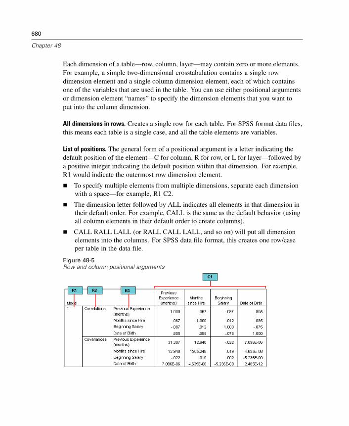
680

Chapter 48

Each dimension of a table—row, column, layer—may contain zero or more elements.For example, a simple two-dimensional crosstabulation contains a single rowdimension element and a single column dimension element, each of which containsone of the variables that are used in the table. You can use either positional argumentsor dimension element “names” to specify the dimension elements that you want toput into the column dimension.

All dimensions in rows. Creates a single row for each table. For SPSS format data files,this means each table is a single case, and all the table elements are variables.

List of positions. The general form of a positional argument is a letter indicating thedefault position of the element—C for column, R for row, or L for layer—followed bya positive integer indicating the default position within that dimension. For example,R1 would indicate the outermost row dimension element.

To specify multiple elements from multiple dimensions, separate each dimensionwith a space—for example, R1 C2.

The dimension letter followed by ALL indicates all elements in that dimension intheir default order. For example, CALL is the same as the default behavior (usingall column elements in their default order to create columns).

CALL RALL LALL (or RALL CALL LALL, and so on) will put all dimensionelements into the columns. For SPSS data file format, this creates one row/caseper table in the data file.

Figure 48-5Row and column positional arguments

681


List of dimension names. As an alternative to positional arguments, you can usedimension element “names,” which are the text labels that appear in the table. Forexample, a simple two-dimensional crosstabulation contains a single row dimensionelement and a single column dimension element, each with labels based on thevariables in those dimensions, plus a single layer dimension element labeled Statistics(if English is the output language).

Dimension element names may vary, based on the output language and/or settingsthat affect the display of variable names and/or labels in tables.

Each dimension element name must be enclosed in single or double quotationmarks. To specify multiple dimension element names, include a space betweeneach quoted name.

The labels that are associated with the dimension elements may not always be obvious.

To See All Dimension Elements and Their Labels for a Pivot Table

E Activate (double-click) the table in the Viewer.


Show All

and/or

E If the pivoting trays aren’t displayed, from the menus choose:Pivot

Pivoting Trays

E Hover the pointer over each icon in the pivoting trays to display the label.

682

Chapter 48

Figure 48-6Dimension element names displayed in table and pivoting trays

LoggingYou can record OMS activity in a log in XML or text format.

The log tracks all new OMS requests for the session but does not include OMSrequests that were already active before you requested a log.

The current log file ends if you specify a new log file or if you deselect (uncheck)Log OMS activity.

To specify OMS logging:

E Click Logging in the Output Management System Control Panel.

683


Excluding Output Display from the Viewer

The Exclude from Viewer check box affects all output that is selected in the OMSrequest by suppressing the display of that output in the Viewer window. This processis often useful for production jobs that generate a lot of output and when you don’tneed the results in the form of a Viewer document (.spo file). You can also use thisfunctionality to suppress the display of particular output objects that you simply neverwant to see, without routing any other output to some external file and format.

To suppress the display of certain output objects without routing other output to anexternal file:

E Create an OMS request that identifies the unwanted output.

E Select Exclude from Viewer.

E For the output destination, select File—but leave the File field blank.

E Click Add.

The selected output will be excluded from the Viewer while all other output will bedisplayed in the Viewer in the normal fashion.

Routing Output to SPSS Data Files

An SPSS data file consists of variables in the columns and cases in the rows, which isessentially the format in which pivot tables are converted to data files:

Columns in the table are variables in the data file. Valid variable names areconstructed from the column labels.

Row labels in the table become variables with generic variable names (Var1, Var2,Var3, and so on) in the data file. The values of these variables are the row labelsin the table.

Three table-identifier variables are automatically included in the data file:Command_, Subtype_, and Label_. All three are string variables. The firsttwo variables correspond to the command and subtype identifiers. For moreinformation, see “Command Identifiers and Table Subtypes” on p. 675. Label_contains the table title text.

Rows in the table become cases in the data file.

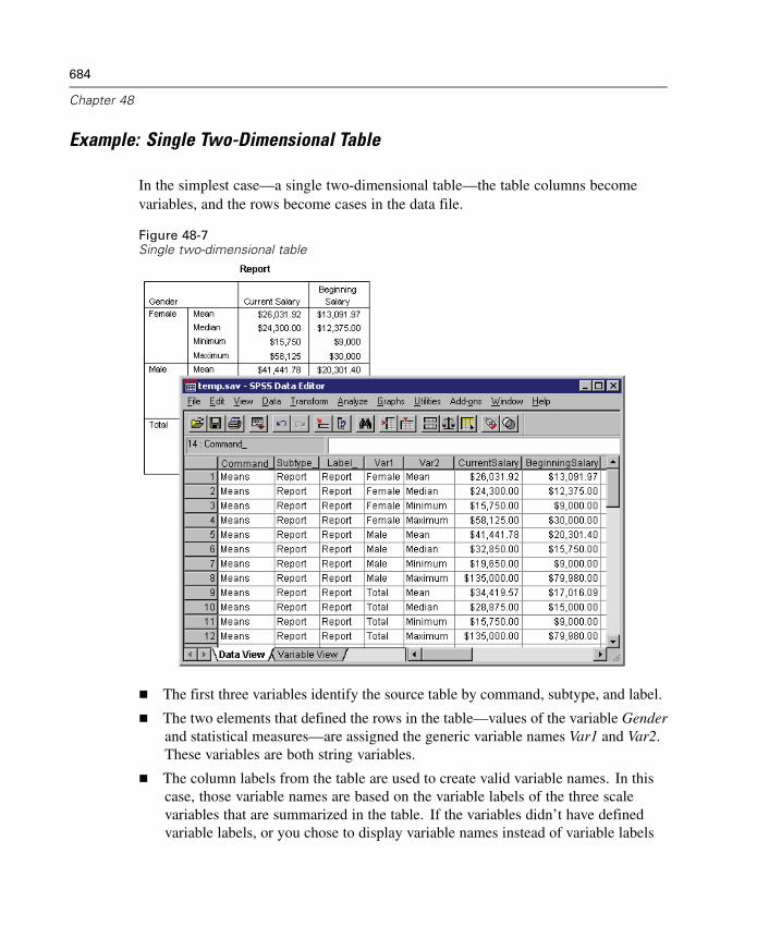
684

Chapter 48

Example: Single Two-Dimensional Table

In the simplest case—a single two-dimensional table—the table columns becomevariables, and the rows become cases in the data file.

Figure 48-7Single two-dimensional table

The first three variables identify the source table by command, subtype, and label.

The two elements that defined the rows in the table—values of the variable Genderand statistical measures—are assigned the generic variable names Var1 and Var2.These variables are both string variables.

The column labels from the table are used to create valid variable names. In thiscase, those variable names are based on the variable labels of the three scalevariables that are summarized in the table. If the variables didn’t have definedvariable labels, or you chose to display variable names instead of variable labels

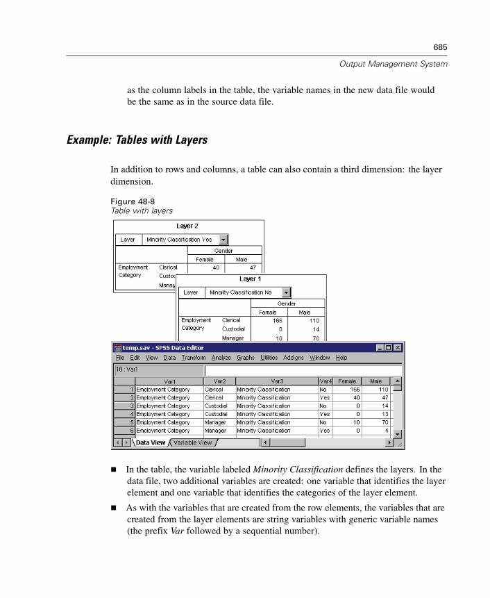
685


as the column labels in the table, the variable names in the new data file wouldbe the same as in the source data file.

Example: Tables with Layers

In addition to rows and columns, a table can also contain a third dimension: the layerdimension.

Figure 48-8Table with layers

In the table, the variable labeled Minority Classification defines the layers. In thedata file, two additional variables are created: one variable that identifies the layerelement and one variable that identifies the categories of the layer element.

As with the variables that are created from the row elements, the variables that arecreated from the layer elements are string variables with generic variable names(the prefix Var followed by a sequential number).

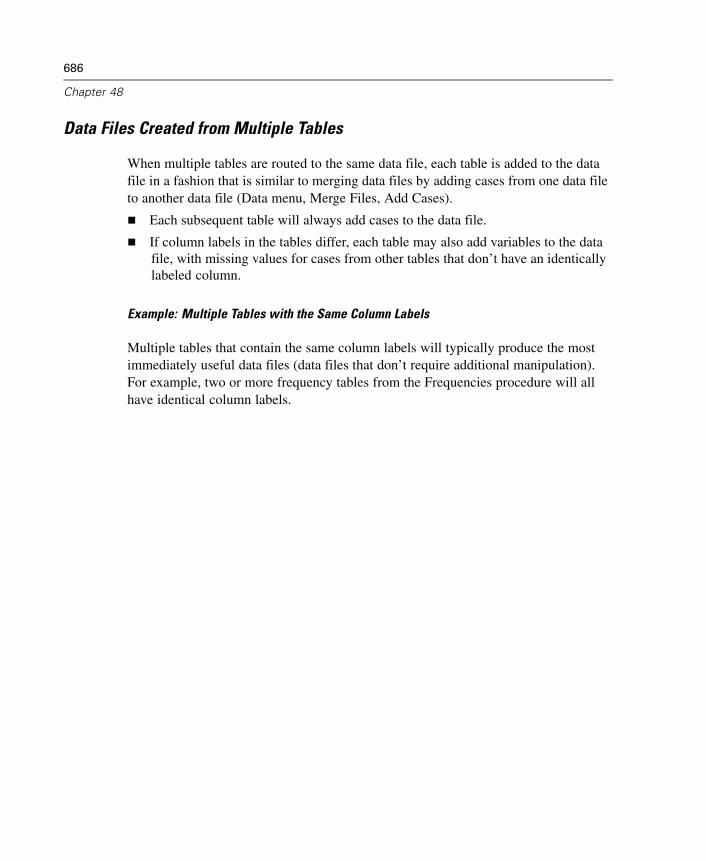
686

Chapter 48

Data Files Created from Multiple Tables

When multiple tables are routed to the same data file, each table is added to the datafile in a fashion that is similar to merging data files by adding cases from one data fileto another data file (Data menu, Merge Files, Add Cases).

Each subsequent table will always add cases to the data file.

If column labels in the tables differ, each table may also add variables to the datafile, with missing values for cases from other tables that don’t have an identicallylabeled column.

Example: Multiple Tables with the Same Column Labels

Multiple tables that contain the same column labels will typically produce the mostimmediately useful data files (data files that don’t require additional manipulation).For example, two or more frequency tables from the Frequencies procedure will allhave identical column labels.

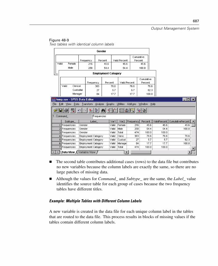
687


Figure 48-9Two tables with identical column labels

The second table contributes additional cases (rows) to the data file but contributesno new variables because the column labels are exactly the same, so there are nolarge patches of missing data.

Although the values for Command_ and Subtype_ are the same, the Label_ valueidentifies the source table for each group of cases because the two frequencytables have different titles.

Example: Multiple Tables with Different Column Labels

A new variable is created in the data file for each unique column label in the tablesthat are routed to the data file. This process results in blocks of missing values if thetables contain different column labels.

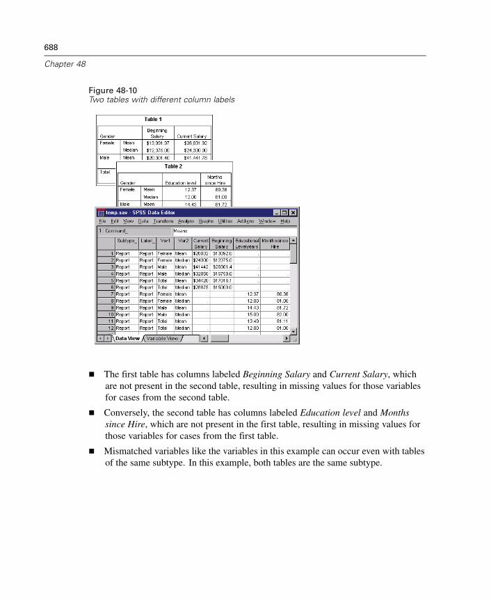
688

Chapter 48

Figure 48-10Two tables with different column labels

The first table has columns labeled Beginning Salary and Current Salary, whichare not present in the second table, resulting in missing values for those variablesfor cases from the second table.

Conversely, the second table has columns labeled Education level and Monthssince Hire, which are not present in the first table, resulting in missing values forthose variables for cases from the first table.

Mismatched variables like the variables in this example can occur even with tablesof the same subtype. In this example, both tables are the same subtype.

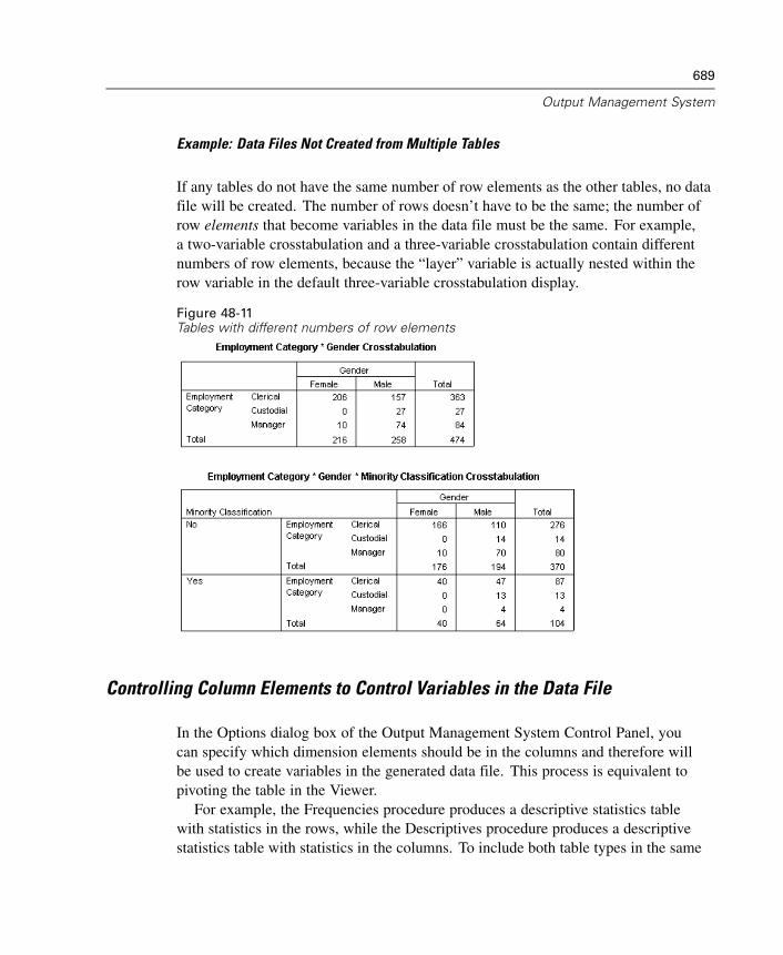
689


Example: Data Files Not Created from Multiple Tables

If any tables do not have the same number of row elements as the other tables, no datafile will be created. The number of rows doesn’t have to be the same; the number ofrow elements that become variables in the data file must be the same. For example,a two-variable crosstabulation and a three-variable crosstabulation contain differentnumbers of row elements, because the “layer” variable is actually nested within therow variable in the default three-variable crosstabulation display.

Figure 48-11Tables with different numbers of row elements

Controlling Column Elements to Control Variables in the Data File

In the Options dialog box of the Output Management System Control Panel, youcan specify which dimension elements should be in the columns and therefore willbe used to create variables in the generated data file. This process is equivalent topivoting the table in the Viewer.

For example, the Frequencies procedure produces a descriptive statistics tablewith statistics in the rows, while the Descriptives procedure produces a descriptivestatistics table with statistics in the columns. To include both table types in the same

690

Chapter 48

data file in a meaningful fashion, you need to change the column dimension for oneof the table types.

Because both table types use the element name “Statistics” for the statisticsdimension, we can put the statistics from the Frequencies statistics table in the columnssimply by specifying “Statistics” (in quotation marks) in the list of dimension names inthe OMS Options dialog box.

Figure 48-12OMS Options dialog box

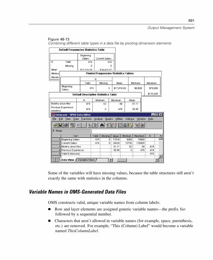
691


Figure 48-13Combining different table types in a data file by pivoting dimension elements

Some of the variables will have missing values, because the table structures still aren’texactly the same with statistics in the columns.

Variable Names in OMS-Generated Data Files

OMS constructs valid, unique variable names from column labels:

Row and layer elements are assigned generic variable names—the prefix Varfollowed by a sequential number.

Characters that aren’t allowed in variable names (for example, space, parenthesis,etc.) are removed. For example, “This (Column) Label” would become a variablenamed ThisColumnLabel.

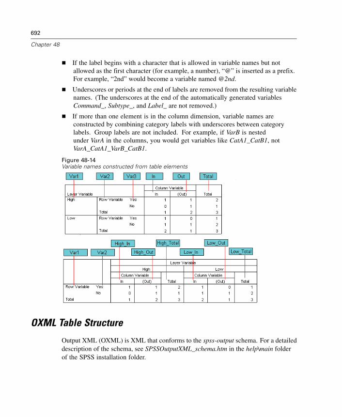
692

Chapter 48

If the label begins with a character that is allowed in variable names but notallowed as the first character (for example, a number), “@” is inserted as a prefix.For example, “2nd” would become a variable named @2nd.

Underscores or periods at the end of labels are removed from the resulting variablenames. (The underscores at the end of the automatically generated variablesCommand_, Subtype_, and Label_ are not removed.)

If more than one element is in the column dimension, variable names areconstructed by combining category labels with underscores between categorylabels. Group labels are not included. For example, if VarB is nestedunder VarA in the columns, you would get variables like CatA1_CatB1, notVarA_CatA1_VarB_CatB1.

Figure 48-14Variable names constructed from table elements

OXML Table Structure

Output XML (OXML) is XML that conforms to the spss-output schema. For a detaileddescription of the schema, see SPSSOutputXML_schema.htm in the help\main folderof the SPSS installation folder.

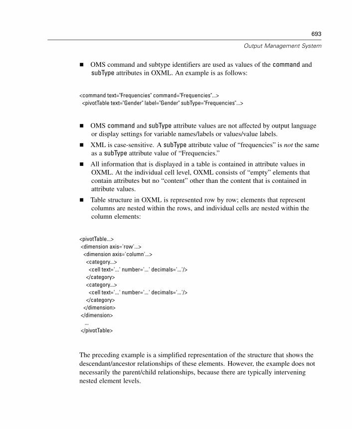
693


OMS command and subtype identifiers are used as values of the command andsubType attributes in OXML. An example is as follows:

<command text="Frequencies" command="Frequencies"...><pivotTable text="Gender" label="Gender" subType="Frequencies"...>

OMS command and subType attribute values are not affected by output languageor display settings for variable names/labels or values/value labels.

XML is case-sensitive. A subType attribute value of “frequencies” is not the sameas a subType attribute value of “Frequencies.”

All information that is displayed in a table is contained in attribute values inOXML. At the individual cell level, OXML consists of “empty” elements thatcontain attributes but no “content” other than the content that is contained inattribute values.

Table structure in OXML is represented row by row; elements that representcolumns are nested within the rows, and individual cells are nested within thecolumn elements:

<pivotTable...><dimension axis='row'...><dimension axis='column'...>

<category...><cell text='...' number='...' decimals='...'/>

</category><category...>

<cell text='...' number='...' decimals='...'/></category>

</dimension></dimension>

...</pivotTable>

The preceding example is a simplified representation of the structure that shows thedescendant/ancestor relationships of these elements. However, the example does notnecessarily the parent/child relationships, because there are typically interveningnested element levels.

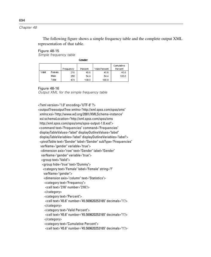
694

Chapter 48

The following figure shows a simple frequency table and the complete output XMLrepresentation of that table.

Figure 48-15Simple frequency table

Figure 48-16Output XML for the simple frequency table

<?xml version="1.0" encoding="UTF-8" ?><outputTreeoutputTree xmlns="http://xml.spss.com/spss/oms"

xmlns:xsi="http://www.w3.org/2001/XMLSchema-instance"xsi:schemaLocation="http://xml.spss.com/spss/omshttp://xml.spss.com/spss/oms/spss-output-1.0.xsd"><command text="Frequencies" command="Frequencies"displayTableValues="label" displayOutlineValues="label"displayTableVariables="label" displayOutlineVariables="label"><pivotTable text="Gender" label="Gender" subType="Frequencies"varName="gender" variable="true"><dimension axis="row" text="Gender" label="Gender"varName="gender" variable="true"><group text="Valid"><group hide="true" text="Dummy"><category text="Female" label="Female" string="f"varName="gender"><dimension axis="column" text="Statistics"><category text="Frequency"><cell text="216" number="216"/></category><category text="Percent"><cell text="45.6" number="45.569620253165" decimals="1"/></category><category text="Valid Percent"><cell text="45.6" number="45.569620253165" decimals="1"/>

</category><category text="Cumulative Percent"><cell text="45.6" number="45.569620253165" decimals="1"/>

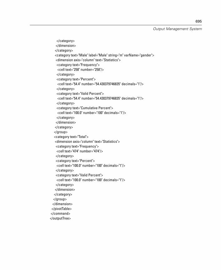
695


</category></dimension>

</category><category text="Male" label="Male" string="m" varName="gender"><dimension axis="column" text="Statistics"><category text="Frequency"><cell text="258" number="258"/></category><category text="Percent"><cell text="54.4" number="54.430379746835" decimals="1"/>

</category><category text="Valid Percent"><cell text="54.4" number="54.430379746835" decimals="1"/>

</category><category text="Cumulative Percent"><cell text="100.0" number="100" decimals="1"/></category></dimension>

</category></group><category text="Total"><dimension axis="column" text="Statistics"><category text="Frequency"><cell text="474" number="474"/></category><category text="Percent"><cell text="100.0" number="100" decimals="1"/></category><category text="Valid Percent"><cell text="100.0" number="100" decimals="1"/></category>

</dimension></category></group>

</dimension></pivotTable></command>

</outputTree>

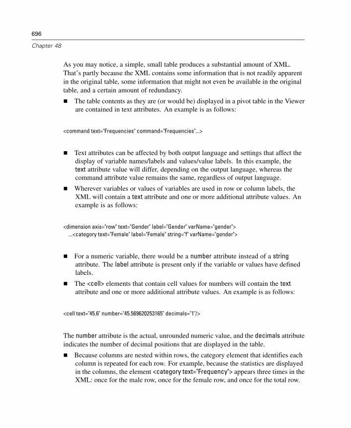
696

Chapter 48

As you may notice, a simple, small table produces a substantial amount of XML.That’s partly because the XML contains some information that is not readily apparentin the original table, some information that might not even be available in the originaltable, and a certain amount of redundancy.

The table contents as they are (or would be) displayed in a pivot table in the Viewerare contained in text attributes. An example is as follows:

<command text="Frequencies" command="Frequencies"...>

Text attributes can be affected by both output language and settings that affect thedisplay of variable names/labels and values/value labels. In this example, thetext attribute value will differ, depending on the output language, whereas thecommand attribute value remains the same, regardless of output language.

Wherever variables or values of variables are used in row or column labels, theXML will contain a text attribute and one or more additional attribute values. Anexample is as follows:

<dimension axis="row" text="Gender" label="Gender" varName="gender">...<category text="Female" label="Female" string="f" varName="gender">

For a numeric variable, there would be a number attribute instead of a stringattribute. The label attribute is present only if the variable or values have definedlabels.

The <cell> elements that contain cell values for numbers will contain the textattribute and one or more additional attribute values. An example is as follows:

<cell text="45.6" number="45.569620253165" decimals="1"/>

The number attribute is the actual, unrounded numeric value, and the decimals attributeindicates the number of decimal positions that are displayed in the table.

Because columns are nested within rows, the category element that identifies eachcolumn is repeated for each row. For example, because the statistics are displayedin the columns, the element <category text="Frequency"> appears three times in theXML: once for the male row, once for the female row, and once for the total row.

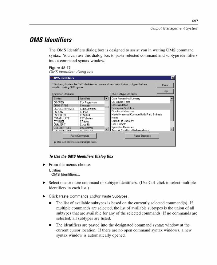
697


OMS IdentifiersThe OMS Identifiers dialog box is designed to assist you in writing OMS commandsyntax. You can use this dialog box to paste selected command and subtype identifiersinto a command syntax window.

Figure 48-17OMS Identifiers dialog box

To Use the OMS Identifiers Dialog Box


OMS Identifiers...

E Select one or more command or subtype identifiers. (Use Ctrl-click to select multipleidentifiers in each list.)

E Click Paste Commands and/or Paste Subtypes.

The list of available subtypes is based on the currently selected command(s). Ifmultiple commands are selected, the list of available subtypes is the union of allsubtypes that are available for any of the selected commands. If no commands areselected, all subtypes are listed.

The identifiers are pasted into the designated command syntax window at thecurrent cursor location. If there are no open command syntax windows, a newsyntax window is automatically opened.

698

Chapter 48

Each command and/or subtype identifier is enclosed in quotation marks whenpasted, because OMS command syntax requires these quotation marks.

Identifier lists for the COMMANDS and SUBTYPES keywords must be enclosed inbrackets, as in:

/IF COMMANDS=['Crosstabs' 'Descriptives']SUBTYPES=['Crosstabulation' 'Descriptive Statistics']

Copying OMS Identifiers from the Viewer Outline

You can copy and paste OMS command and subtype identifiers from the Vieweroutline pane.

E In the outline pane, right-click the outline entry for the item.

E Choose Copy OMS Command Identifier or Copy OMS Table Subtype.

This method differs from the OMS Identifiers dialog box method in one respect:The copied identifier is not automatically pasted into a command syntax window.The identifier is simply copied to the clipboard, and you can then paste it anywhereyou want. Because command and subtype identifier values are identical to thecorresponding command and subtype attribute values in XML-format output (OXML),you might find this copy/paste method useful if you write XSLT transformations.

Copying OMS Labels

Instead of identifiers, you can copy labels for use with the LABELS keyword. Labelscan be used to differentiate between multiple graphs or multiple tables of the sametype in which the outline text reflects some attribute of the particular output object,such as the variable names or labels. There are, however, a number of factors thatcan affect the label text:

If split-file processing is on, split-file group identification may be appended tothe label.

699


Labels that include information about variables or values are affected by thesettings for the display of variable names/labels and values/value labels in theoutline pane (Edit menu, Options, Output Labels tab).

Labels are affected by the current output language setting (Edit menu, Options,General tab).

To copy OMS labels

E In the outline pane, right-click the outline entry for the item.

E Choose Copy OMS Label.

As with command and subtype identifiers, the labels must be in quotation marks, andthe entire list must be enclosed in square brackets, as in:

/IF LABELS=['Employment Category' 'Education Level']

Appendix

ADatabase Access Administrator

The Database Access Administrator is a utility designed to simplify large or confusingdata sources for use with the Database Wizard. The Database Access Administratorallows users and administrators to customize their data sources in the following ways:

Create aliases for database tables and fields.

Create variable names for fields.

Hide extraneous tables and fields.

The Database Access Administrator does not actually change your database. Instead, itgenerates files that hold all of your information. These files act as database views.

You can use the Database Access Administrator to specify up to three differentviews per database: enterprise level, department level, and personal level. Both theDatabase Access Administrator and the Database Wizard recognize these files by thefollowing names:

Enterprise level: dba01.inf

Department level: dba02.inf

Personal level: dba03.inf

Each file contains level-specific information about any number of data sources. Forexample, your dba03.inf file could contain personal view information for a corporateaccounts database, your company’s hourlog database, and a database that you use tokeep track of your CD collection.

When you open the Database Access Administrator, it will search your system’spath for these files and automatically display information for all three views of anydata source that you have configured.

Inheritance and priorities. Whenever you use the Database Wizard, it presents thelowest-level view of your data source that it can find on your system’s path, wherethe levels are (from highest to lowest) enterprise, department, and personal. Each

701

702

Appendix A

level’s file holds information about all of your data sources for that level. For example,your marketing department will have one file, dba02.inf, that contains the aliasinginformation for all of the database views that are established for the marketingdepartment. Each person in the marketing department will have a file, dba03.inf, thatcontains customized views of all of the databases that he or she uses.

In the Database Access Administrator, aliases, variable names, and hide ordersare inherited from the top down.

Examples:

If the Regions table is hidden at the enterprise level, it is invisible at both thedepartment and personal levels. This table would not be displayed in the DatabaseWizard.

The field JOBCAT in the Employee Sales table is not aliased at the enterpriselevel, but it is aliased as Job Categories at the department level. It appearsas Job Categories at the personal level. Additionally, if the Employee Salestable is aliased as Employee Information at the personal level, the original field(EmployeeSales.JOBCAT) would appear in the Database Wizard as ’EmployeeInformation’.’Job Categories’.

To start the Database Access Administrator, run the file spssdbca.exe, which isinstalled in your SPSS directory. For more information about the Database AccessAdministrator, see the online Help.

Appendix

BCustomizing HTML Documents

You can automatically add customized HTML code to documents exported in HTMLformat, including:

HTML document titles

Document type specification

Meta-tags and script code (for example, JavaScript)

Text displayed before and after exported output

To Add Customized HTML Code to Exported Output DocumentsE In a text editor, open the file htmlfram.txt (located in the directory in which SPSS is

installed).

E In the “fields” on the lines between the double open brackets (<<), replace thecomments with the text or HTML code that you want to insert into your exportedHTML documents.

E Save the file as a text file.

Note: If you change the name or location of the text file, you have to modify the systemregistry to use the file to customize your exported HTML output.

Content and Format of the Text File for Customized HTML

The HTML code that you want to add automatically to your HTML documents mustbe specified in a simple text file that contains six fields, each field delimited by twoopen angle brackets on the preceding line (<<):

<<

703

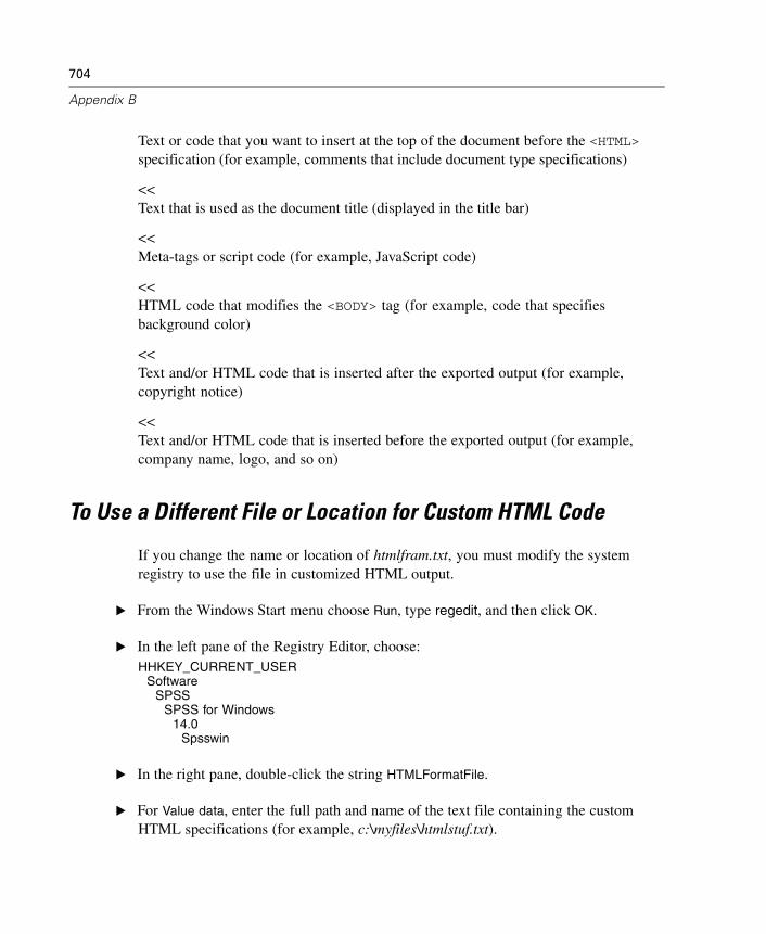
704

Appendix B

Text or code that you want to insert at the top of the document before the <HTML>specification (for example, comments that include document type specifications)

<<Text that is used as the document title (displayed in the title bar)

<<Meta-tags or script code (for example, JavaScript code)

<<HTML code that modifies the <BODY> tag (for example, code that specifiesbackground color)

<<Text and/or HTML code that is inserted after the exported output (for example,copyright notice)

<<Text and/or HTML code that is inserted before the exported output (for example,company name, logo, and so on)

To Use a Different File or Location for Custom HTML Code

If you change the name or location of htmlfram.txt, you must modify the systemregistry to use the file in customized HTML output.

E From the Windows Start menu choose Run, type regedit, and then click OK.

E In the left pane of the Registry Editor, choose:HHKEY_CURRENT_USER

SoftwareSPSS

SPSS for Windows14.0

Spsswin

E In the right pane, double-click the string HTMLFormatFile.

E For Value data, enter the full path and name of the text file containing the customHTML specifications (for example, c:\myfiles\htmlstuf.txt).

705

Customizing HTML Documents

Sample Text File for Customized HTML

<<<!DOCTYPE HTML PUBLIC "-//W3C//DTD HTML 3.2//EN"><<NVI, Inc.<<<META NAME="keywords" CONTENT="gizmos, gadgets, gimcracks"><<bgcolor="#FFFFFF"<<<H4 align=center>This page made possible by...<br><br><IMG SRC="spss2.gif" align=center></H4><<<h2 align=center>NVI Sales</h2><h3 align=center>Regional Data</h3>

Sample HTML Source for Customized HTML

<!DOCTYPE HTML PUBLIC "-//W3C//DTD HTML 3.2//EN"><HTML><HEAD><TITLE>NVI Sales, Inc.</TITLE><META NAME="keywords" CONTENT="gizmos, gadgets, gimcracks"></HEAD><BODY bgcolor="#FFFFFF"><h2 align=center>NVI Sales</h2><h3 align=center>Regional Data</h3>

[Exported output]

<H4 align=center>This page made possible by...<br><br><IMG SRC="spss2.gif" align=center></H4></BODY></HTML>

Index

Access (Microsoft), 28active file, 68, 70

caching, 70creating a temporary active file, 70virtual active file, 68

active window, 7ActiveX objects, 248adding group labels, 284adjusted R2

in Linear Regression, 436aggregating data, 203

aggregate functions, 206variable names and labels, 207

algorithms, 15alignment, 96, 243, 306, 598

in cells, 306in Data Editor, 96output, 243, 598

alpha coefficient

in Reliability Analysis, 553, 555alpha factoring, 463analysis of variance

in Curve Estimation, 441in Linear Regression, 436in Means, 358in One-Way ANOVA, 379

Anderson-Rubin factor scores, 466Andrews’ wave estimator

in Explore, 334ANOVA

in GLM Univariate, 389in Means, 358

in One-Way ANOVA, 379model, 393

aspect ratio, 603automated production, 623automation objects, 649, 652–653, 655–656

methods, 655object browser, 656properties, 655types, 652using in scripts, 649, 653, 656variable-naming conventions, 652

autoscripts, 613, 646, 648autoscript file, 649creating, 646trigger events, 648

average absolute deviation (AAD)

in Ratio Statistics, 569

backward elimination

in Linear Regression, 430banding data values, 135bar charts

in Frequencies, 325Bartlett factor scores, 466Bartlett’s test of sphericity

in Factor Analysis, 462beta coefficients

in Linear Regression, 436Binomial Test, 502

command additional features, 504dichotomies, 502missing values, 504

707

708

Index

options, 504statistics, 504


command additional features, 411correlation coefficients, 407missing values, 410options, 410significance level, 407statistics, 410

block distance

in Distances, 421Blom estimates, 160BMP files, 251, 257–258, 625

exporting charts, 251, 257–258, 625Bonferroni

in GLM, 398in One-Way ANOVA, 383

bookmarking pivot table views, 289bookmarks, 289borders, 273, 299–300

displaying hidden borders, 300Draft Viewer, 273

Box’s M test

in Discriminant Analysis, 451boxplots

comparing factor levels, 335comparing variables, 335in Explore, 335

break points, 664in scripts, 664

break variables

in Aggregate Data, 203Brown-Forsythe statistic

in One-Way ANOVA, 385build terms, 394buttons, 620

editing toolbar bitmap icons, 620

caching, 70active file, 70

Cancel button, 10captions, 310

adding to a table, 310case-control study

Paired-Samples T Test, 373cases, 102–103, 215

finding duplicates, 132finding in Data Editor, 103inserting new cases, 102restructuring into variables, 215selecting subsets, 209, 211–212sorting, 193weighing, 213

casewise diagnostics

in Linear Regression, 436categorical data, 116

converting interval data to discrete categories,135

cell borders, 273Draft Viewer, 273

cells in pivot tables, 292, 297, 301–302, 304,306–307, 310

alignment, 306fonts, 301formats, 297hiding, 290margins, 307modifying text, 310outlines, 307shading, 307showing, 290value formats, 304widths, 302

centered moving average function, 184centering output, 243, 598

709

Index

chart options, 603charts, 241, 247, 249, 251, 603, 625

aspect ratio, 603case labels, 441copying, 247copying into other applications, 247creating, 571exporting, 251, 625footnotes, 579hiding, 241in ROC Curve, 585missing values, 580modifying, 575overview, 571pasting into other applications, 249subtitles, 579templates, 582, 603titles, 579

Chebychev distance

in Distances, 421chi-square, 498

expected range, 500expected values, 500Fisher’s exact test, 342for independence, 342in Crosstabs, 342likelihood-ratio, 342linear-by-linear association, 342missing values, 501one-sample test, 498options, 501Pearson, 342statistics, 501Yates’ correction for continuity, 342

chi-square distance

in Distances, 421

classification

in ROC Curve, 585cluster analysis

efficiency, 493Hierarchical Cluster Analysis, 481K-Means Cluster Analysis, 489

cluster frequencies

in TwoStep Cluster Analysis, 479clustering

choosing a procedure, 469Cochran’s Q

in Tests for Several Related Samples, 524Cochran’s statistic

in Crosstabs, 342coefficient of dispersion (COD)

in Ratio Statistics, 569coefficient of variation (COV)

in Ratio Statistics, 569Cohen’s kappa

in Crosstabs, 342collapsing categories, 135collinearity diagnostics

in Linear Regression, 436colors in pivot tables, 299, 301, 307

borders, 299cell background, 307cell foreground, 307font, 301

column format, 305changing in pivot tables, 305

column percentages

in Crosstabs, 345column summary reports, 545column width, 95, 295, 303, 608

controlling default width, 608controlling maximum width, 295controlling width for wrapped text, 295

710

Index

in Data Editor, 95pivot tables, 303

columns, 303, 309changing width in pivot tables, 303selecting in pivot tables, 309

comma format, 90, 92comma-delimited data, 44command identifiers, 675command language, 313command line switches, 634

Production Facility, 634command syntax, 313, 319, 596, 598–599, 615,

619, 623accessing SPSS Command Syntax Reference, 15adding to menus, 615journal file, 318, 320, 596log, 598–599output log, 316pasting, 315Production Facility formatting, 633Production Facility rules, 623running, 319running with toolbar buttons, 619syntax rules, 313

comparing groups

in OLAP Cubes, 367comparing variables

in OLAP Cubes, 367compound model

in Curve Estimation, 445computing variables, 145

computing new string variables, 148concentration index

in Ratio Statistics, 569conditional transformations, 147confidence intervals

in Explore, 334

in GLM, 395, 403in Independent-Samples T Test, 373in Linear Regression, 436in One-Sample T Test, 378in One-Way ANOVA, 385in Paired-Samples T Test, 375in ROC Curve, 588saving in Linear Regression, 433

context-sensitive Help, 285finding label definitions in pivot tables, 285

contingency coefficient

in Crosstabs, 342contingency tables, 339continuation text, 301

for pivot tables, 301contrasts

in GLM, 395–396in One-Way ANOVA, 382

control variables

in Crosstabs, 341convergence

in Factor Analysis, 463, 465in K-Means Cluster Analysis, 494

Cook’s distance

in GLM, 401in Linear Regression, 433

copying, 242, 247charts, 247output, 242pivot tables, 247

correlation matrix

in Discriminant Analysis, 451in Factor Analysis, 457, 462

correlations

in Bivariate Correlations, 407in Crosstabs, 342in Partial Correlations, 413

711

Index

zero-order, 416counting occurrences, 150covariance matrix

in Discriminant Analysis, 451, 454in GLM, 401in Linear Regression, 436

covariance ratio

in Linear Regression, 433Cramér’s V

in Crosstabs, 342Cronbach’s alpha

in Reliability Analysis, 553, 555Crosstabs, 339

cell display, 345clustered bar charts, 342control variables, 341formats, 347fractional weights, 213layers, 341statistics, 342suppressing tables, 339

crosstabulation

in Crosstabs, 339multiple response, 532

CSV-format data, 44cubic model

in Curve Estimation, 445cumulative sum function, 184currency formats, 611Curve Estimation, 441

analysis of variance, 441forecast, 446including constant, 441models, 445saving predicted values, 446saving prediction intervals, 446saving residuals, 446

custom currency formats, 90, 611custom models

in GLM, 393

d

in Crosstabs, 342data analysis, 12

basic steps, 12data dictionary

applying from another file, 122Data Editor, 85, 88, 95–96, 98–104, 106, 615

alignment, 96changing data type, 103column width, 95data value restrictions, 99Data View, 86defining variables, 88display options, 104editing data, 100–101entering data, 98entering non-numeric data, 99entering numeric data, 99filtered cases, 104finding cases, 103inserting new cases, 102inserting new variables, 102moving variables, 103multiple open data files, 107multiple views/panes, 104printing, 106sending data to other applications, 615Variable View, 87

data entry, 98data files, 23–24, 44, 59–60, 64–65, 67, 70,

78–80, 215adding comments, 590dictionary information, 59–60

712

Index

Dimensions, 55file information, 59–60flipping, 194improving performance for large files, 70mrInterview, 55multiple open data files, 107opening, 23–24protecting, 68Quancept, 55Quanvert, 55remote servers, 78–80restructuring, 215saving, 60, 64–65saving output as SPSS-format data files, 669saving subsets of variables, 67text, 44transposing, 194

Data List, 68versus Get Data command, 68

data transformations, 610computing variables, 145conditional transformations, 147delaying execution, 610functions, 148ranking cases, 158recoding values, 153–155, 157, 162string variables, 148time series, 180, 183

data types, 90, 92, 103, 611changing, 103custom currency, 90, 611defining, 90display formats, 92input formats, 92

Data View, 86database files, 27–28, 32, 34–36, 38, 41, 43

conditional expressions, 36

converting strings to numeric variables, 41creating relationships, 34database security, 32defining variables, 41logging into a database, 32Microsoft Access, 28parameter queries, 36, 38Prompt for Value, 38random sampling, 36reading, 27–28, 32relationship properties, 35saving queries, 43selecting a data source, 28selecting data fields, 32specifying criteria, 36SQL syntax, 43table joins, 34–35verifying results, 43Where clause, 36

datasets

renaming, 110date formats, 90, 92, 610

two-digit years, 610date variables

add or subtract from date/time variables, 165create date/time variable from set of variables,

165create date/time variable from string, 165defining for time series data, 181extract part of date/time variable, 165

dBASE files, 23, 26, 64–65opening, 23, 26saving, 64–65

debugging scripts, 664–665break points, 664debugging pane, 665stepping through scripts, 664

713

Index

Define Multiple Response Sets, 528categories, 528dichotomies, 528set labels, 528set names, 528

defining variables, 88, 90, 92–94, 96–97, 112applying a data dictionary, 122copying and pasting attributes, 96–97data types, 90missing values, 94templates, 96–97value labels, 93, 112variable labels, 92

deleted residuals


deleting multiple EXECUTES in syntax files, 320deleting output, 242dendrograms

in Hierarchical Cluster Analysis, 486dependent t test

in Paired-Samples T Test, 373descriptive statistics

in Descriptives, 327in Explore, 334in Frequencies, 323in GLM Univariate, 403in Ratio Statistics, 569in Summarize, 352in TwoStep Cluster Analysis, 479

Descriptives, 327command additional features, 330display order, 329saving z scores, 327statistics, 329

designated window, 7

detrended normal plots

in Explore, 335deviation contrasts

in GLM, 395–396DfBeta

in Linear Regression, 433DfFit

in Linear Regression, 433dialog boxes, 11, 591–592, 596, 659, 661

controls, 10defining variable sets, 591displaying variable labels, 9, 596displaying variable names, 9, 596optional specifications, 11reordering target lists, 593scripting, 659, 661selecting variables, 11subdialog boxes, 11using variable sets, 592variable display order, 596variable icons, 11variable information, 12variables, 9

dictionary, 59–60difference contrasts

in GLM, 395–396difference function, 184differences between groups

in OLAP Cubes, 367differences between variables

in OLAP Cubes, 367Dimensions data, 55direct oblimin rotation

in Factor Analysis, 465Discriminant Analysis, 447

analyzing held-out cases, 638command additional features, 456

714

Index

covariance matrix, 454criteria, 452defining ranges, 450descriptive statistics, 451discriminant methods, 452display options, 452, 454example, 447exporting model information, 455function coefficients, 451grouping variables, 447independent variables, 447Mahalanobis distance, 452matrices, 451missing values, 454plots, 454prior probabilities, 454Rao’s V, 452saving classification variables, 455selecting cases, 450statistics, 447, 451stepwise methods, 447Wilks’ lambda, 452

disk space, 68, 70temporary, 68, 70

display formats, 92display order, 283distance measures

in Distances, 421in Hierarchical Cluster Analysis, 484

Distances, 419command additional features, 423computing distances between cases, 419computing distances between variables, 419dissimilarity measures, 421example, 419similarity measures, 422statistics, 419

transforming measures, 421–422transforming values, 421–422

distributed mode, 73–75, 78–80, 82, 630available procedures, 82data file access, 78, 80Production Facility, 630saving data files, 79UNC paths, 82

division

dividing across report columns, 548dollar format, 90, 92dollar sign, 305

in pivot tables, 305dot format, 90, 92Draft Viewer, 271–273, 278–279, 596, 599

box characters, 273cell borders, 273changing fonts, 278column borders, 273controlling default output display, 596display options, 599output format, 273printing, 278–279row borders, 273saving output, 279setting default viewer type, 272

Duncan’s multiple range test


Dunnett’s C


Dunnett’s t test


Dunnett’s T3

in GLM, 398

715

Index

in One-Way ANOVA, 383duplicate cases (records)

finding and filtering, 132Durbin-Watson statistic

in Linear Regression, 436

editing data, 100–101effect-size estimates

in GLM Univariate, 403eigenvalues

in Factor Analysis, 462–463in Linear Regression, 436

embedding

interactive charts, 248pivot tables, 248

entering data, 98–99non-numeric, 99numeric, 99using value labels, 99

environment variables, 596SPSSTMPDIR, 596

EPS files, 251, 257, 260, 625exporting charts, 251, 257, 260, 625

equamax rotation

in Factor Analysis, 465estimated marginal means

in GLM Univariate, 403eta

in Crosstabs, 342in Means, 358

eta-squared

in GLM Univariate, 403in Means, 358

Euclidean distance

in Distances, 421Excel files, 23, 25, 64–65, 615

adding menu item to send data to Excel, 615

opening, 23, 25saving, 64–65

Excel format

exporting output, 251, 254excluding output from Viewer with OMS, 683EXECUTE command

pasted from dialog boxes, 320expected count

in Crosstabs, 345Explore, 331

command additional features, 337missing values, 337options, 337plots, 335power transformations, 336statistics, 334

exponential model

in Curve Estimation, 445exporting charts, 251, 257–261, 623, 625

automated production, 623chart size, 257

exporting data, 615adding menu items to export data, 615

exporting output, 251, 255–256, 625, 636Excel format, 251, 254HTML, 254OMS, 669PowerPoint format, 251publishing to Web, 636Word format, 251, 254

extreme values

in Explore, 334

Factor Analysis, 457analyzing held-out cases, 638coefficient display format, 467command additional features, 468

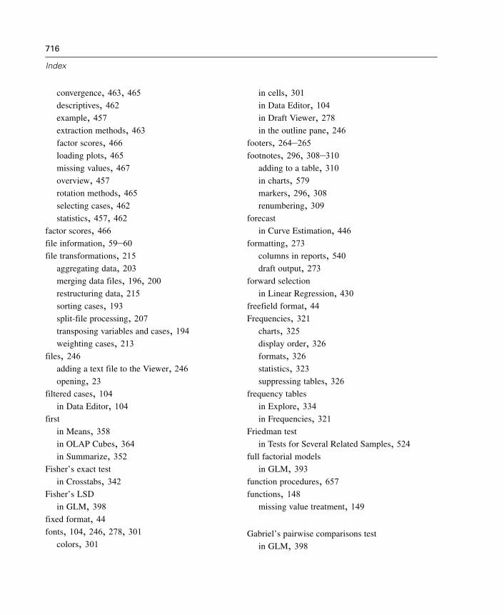
716

Index

convergence, 463, 465descriptives, 462example, 457extraction methods, 463factor scores, 466loading plots, 465missing values, 467overview, 457rotation methods, 465selecting cases, 462statistics, 457, 462

factor scores, 466file information, 59–60file transformations, 215

aggregating data, 203merging data files, 196, 200restructuring data, 215sorting cases, 193split-file processing, 207transposing variables and cases, 194weighting cases, 213

files, 246adding a text file to the Viewer, 246opening, 23

filtered cases, 104in Data Editor, 104

first

in Means, 358in OLAP Cubes, 364in Summarize, 352

Fisher’s exact test

in Crosstabs, 342Fisher’s LSD

in GLM, 398fixed format, 44fonts, 104, 246, 278, 301

colors, 301

in cells, 301in Data Editor, 104in Draft Viewer, 278in the outline pane, 246

footers, 264–265footnotes, 296, 308–310

adding to a table, 310in charts, 579markers, 296, 308renumbering, 309

forecast

in Curve Estimation, 446formatting, 273

columns in reports, 540draft output, 273

forward selection

in Linear Regression, 430freefield format, 44Frequencies, 321

charts, 325display order, 326formats, 326statistics, 323suppressing tables, 326

frequency tables

in Explore, 334in Frequencies, 321

Friedman test

in Tests for Several Related Samples, 524full factorial models

in GLM, 393function procedures, 657functions, 148

missing value treatment, 149

Gabriel’s pairwise comparisons test

in GLM, 398

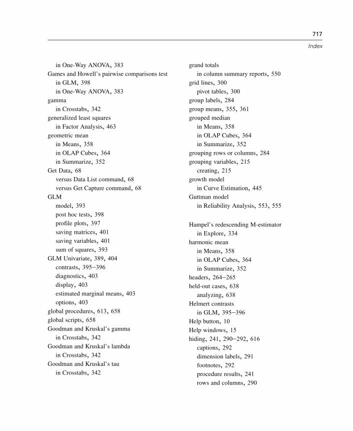
717

Index

in One-Way ANOVA, 383Games and Howell’s pairwise comparisons test


gamma

in Crosstabs, 342generalized least squares

in Factor Analysis, 463geometric mean


Get Data, 68versus Data List command, 68versus Get Capture command, 68

GLM

model, 393post hoc tests, 398profile plots, 397saving matrices, 401saving variables, 401sum of squares, 393

GLM Univariate, 389, 404contrasts, 395–396diagnostics, 403display, 403estimated marginal means, 403options, 403

global procedures, 613, 658global scripts, 658Goodman and Kruskal’s gamma

in Crosstabs, 342Goodman and Kruskal’s lambda

in Crosstabs, 342Goodman and Kruskal’s tau

in Crosstabs, 342

grand totals

in column summary reports, 550grid lines, 300

pivot tables, 300group labels, 284group means, 355, 361grouped median


grouping rows or columns, 284grouping variables, 215

creating, 215growth model

in Curve Estimation, 445Guttman model

in Reliability Analysis, 553, 555

Hampel’s redescending M-estimator

in Explore, 334harmonic mean


headers, 264–265held-out cases, 638

analyzing, 638Helmert contrasts

in GLM, 395–396Help button, 10Help windows, 15hiding, 241, 290–292, 616

captions, 292dimension labels, 291footnotes, 292procedure results, 241rows and columns, 290

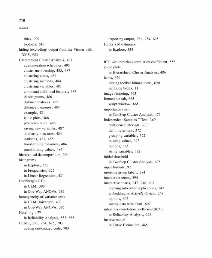
718

Index

titles, 292toolbars, 616

hiding (excluding) output from the Viewer with

OMS, 683Hierarchical Cluster Analysis, 481

agglomeration schedules, 485cluster membership, 485, 487clustering cases, 481clustering methods, 484clustering variables, 481command additional features, 487dendrograms, 486distance matrices, 485distance measures, 484example, 481icicle plots, 486plot orientation, 486saving new variables, 487similarity measures, 484statistics, 481, 485transforming measures, 484transforming values, 484

hierarchical decomposition, 394histograms

in Explore, 335in Frequencies, 325in Linear Regression, 431

Hochberg’s GT2


homogeneity-of-variance tests

in GLM Univariate, 403in One-Way ANOVA, 385

Hotelling’s T2

in Reliability Analysis, 553, 555HTML, 251, 254, 625, 703

adding customized code, 703

exporting output, 251, 254, 625Huber’s M-estimator

in Explore, 334

ICC. See intraclass correlation coefficient, 555icicle plots

in Hierarchical Cluster Analysis, 486icons, 620

editing toolbar bitmap icons, 620in dialog boxes, 11

image factoring, 463Immediate tab, 665

script window, 665importance chart

in TwoStep Cluster Analysis, 477Independent-Samples T Test, 369

confidence intervals, 373defining groups, 372grouping variables, 372missing values, 373options, 373string variables, 372

initial threshold

in TwoStep Cluster Analysis, 475input formats, 92inserting group labels, 284interaction terms, 394interactive charts, 247–248, 607

copying into other applications, 247embedding as ActiveX objects, 248options, 607saving data with chart, 607

intraclass correlation coefficient (ICC)

in Reliability Analysis, 555inverse model

in Curve Estimation, 445

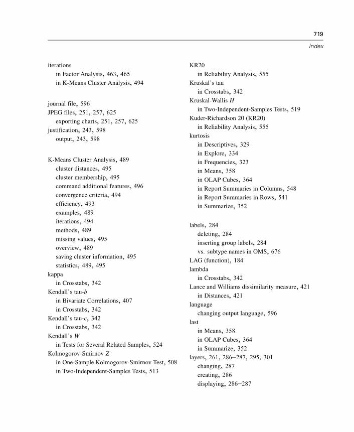
719

Index

iterations

in Factor Analysis, 463, 465in K-Means Cluster Analysis, 494

journal file, 596JPEG files, 251, 257, 625

exporting charts, 251, 257, 625justification, 243, 598

output, 243, 598

K-Means Cluster Analysis, 489cluster distances, 495cluster membership, 495command additional features, 496convergence criteria, 494efficiency, 493examples, 489iterations, 494methods, 489missing values, 495overview, 489saving cluster information, 495statistics, 489, 495

kappa

in Crosstabs, 342Kendall’s tau-b

in Bivariate Correlations, 407in Crosstabs, 342

Kendall’s tau-c, 342in Crosstabs, 342

Kendall’s W

in Tests for Several Related Samples, 524Kolmogorov-Smirnov Z

in One-Sample Kolmogorov-Smirnov Test, 508in Two-Independent-Samples Tests, 513

KR20

in Reliability Analysis, 555Kruskal’s tau

in Crosstabs, 342Kruskal-Wallis H

in Two-Independent-Samples Tests, 519Kuder-Richardson 20 (KR20)

in Reliability Analysis, 555kurtosis

in Descriptives, 329in Explore, 334in Frequencies, 323in Means, 358in OLAP Cubes, 364in Report Summaries in Columns, 548in Report Summaries in Rows, 541in Summarize, 352

labels, 284deleting, 284inserting group labels, 284vs. subtype names in OMS, 676

LAG (function), 184lambda

in Crosstabs, 342Lance and Williams dissimilarity measure, 421

in Distances, 421language

changing output language, 596last


layers, 261, 286–287, 295, 301changing, 287creating, 286displaying, 286–287

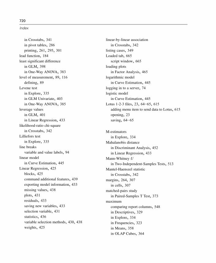
720

Index

in Crosstabs, 341in pivot tables, 286printing, 261, 295, 301

lead function, 184least significant difference


level of measurement, 89, 116defining, 89

Levene test

in Explore, 335in GLM Univariate, 403in One-Way ANOVA, 385

leverage values


likelihood-ratio chi-square

in Crosstabs, 342Lilliefors test

in Explore, 335line breaks

variable and value labels, 94linear model

in Curve Estimation, 445Linear Regression, 425

blocks, 425command additional features, 439exporting model information, 433missing values, 438plots, 431residuals, 433saving new variables, 433selection variable, 431statistics, 436variable selection methods, 430, 438weights, 425

linear-by-linear association

in Crosstabs, 342listing cases, 349Loaded tab, 665

script window, 665loading plots

in Factor Analysis, 465logarithmic model

in Curve Estimation, 445logging in to a server, 74logistic model

in Curve Estimation, 445Lotus 1-2-3 files, 23, 64–65, 615

adding menu item to send data to Lotus, 615opening, 23saving, 64–65

M-estimators

in Explore, 334Mahalanobis distance

in Discriminant Analysis, 452in Linear Regression, 433

Mann-Whitney U

in Two-Independent-Samples Tests, 513Mantel-Haenszel statistic

in Crosstabs, 342margins, 264, 307

in cells, 307matched-pairs study

in Paired-Samples T Test, 373maximum

comparing report columns, 548in Descriptives, 329in Explore, 334in Frequencies, 323in Means, 358in OLAP Cubes, 364

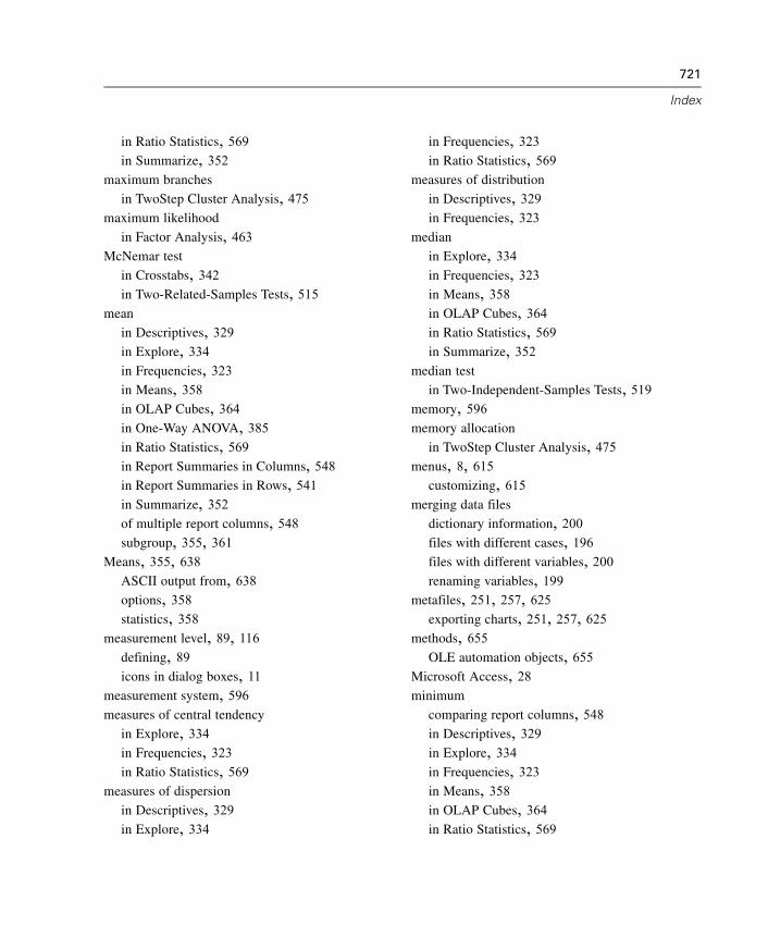
721

Index

in Ratio Statistics, 569in Summarize, 352

maximum branches

in TwoStep Cluster Analysis, 475maximum likelihood

in Factor Analysis, 463McNemar test

in Crosstabs, 342in Two-Related-Samples Tests, 515

mean

in Descriptives, 329in Explore, 334in Frequencies, 323in Means, 358in OLAP Cubes, 364in One-Way ANOVA, 385in Ratio Statistics, 569in Report Summaries in Columns, 548in Report Summaries in Rows, 541in Summarize, 352of multiple report columns, 548subgroup, 355, 361

Means, 355, 638ASCII output from, 638options, 358statistics, 358

measurement level, 89, 116defining, 89icons in dialog boxes, 11

measurement system, 596measures of central tendency

in Explore, 334in Frequencies, 323in Ratio Statistics, 569

measures of dispersion

in Descriptives, 329in Explore, 334

in Frequencies, 323in Ratio Statistics, 569

measures of distribution

in Descriptives, 329in Frequencies, 323

median

in Explore, 334in Frequencies, 323in Means, 358in OLAP Cubes, 364in Ratio Statistics, 569in Summarize, 352

median test

in Two-Independent-Samples Tests, 519memory, 596memory allocation

in TwoStep Cluster Analysis, 475menus, 8, 615

customizing, 615merging data files

dictionary information, 200files with different cases, 196files with different variables, 200renaming variables, 199

metafiles, 251, 257, 625exporting charts, 251, 257, 625

methods, 655OLE automation objects, 655

Microsoft Access, 28minimum

comparing report columns, 548in Descriptives, 329in Explore, 334in Frequencies, 323in Means, 358in OLAP Cubes, 364in Ratio Statistics, 569

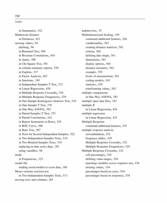
722

Index

in Summarize, 352Minkowski distance

in Distances, 421missing values, 94

defining, 94in Binomial Test, 504in Bivariate Correlations, 410in charts, 580in Chi-Square Test, 501in column summary reports, 550in Explore, 337in Factor Analysis, 467in functions, 149in Independent-Samples T Test, 373in Linear Regression, 438in Multiple Response Crosstabs, 534in Multiple Response Frequencies, 529in One-Sample Kolmogorov-Smirnov Test, 510in One-Sample T Test, 378in One-Way ANOVA, 385in Paired-Samples T Test, 375in Partial Correlations, 416in Report Summaries in Rows, 543in ROC Curve, 588in Runs Test, 507in Tests for Several Independent Samples, 522in Two-Independent-Samples Tests, 514in Two-Related-Samples Tests, 518replacing in time series data, 185string variables, 94

mode

in Frequencies, 323model file

loading saved models to score data, 188Moses extreme reaction test

in Two-Independent-Samples Tests, 513moving rows and columns, 283

mrInterview, 55Multidimensional Scaling, 559

command additional features, 564conditionality, 563creating distance matrices, 562criteria, 564defining data shape, 561dimensions, 563display options, 564distance measures, 562example, 559levels of measurement, 563scaling models, 563statistics, 559transforming values, 562

multiple comparisons

in One-Way ANOVA, 383multiple open data files, 107multiple R

in Linear Regression, 436multiple regression

in Linear Regression, 425Multiple Response

command additional features, 535multiple response analysis

crosstabulation, 532frequency tables, 529Multiple Response Crosstabs, 532Multiple Response Frequencies, 529

Multiple Response Crosstabs, 532cell percentages, 534defining value ranges, 534matching variables across response sets, 534missing values, 534percentages based on cases, 534percentages based on responses, 534

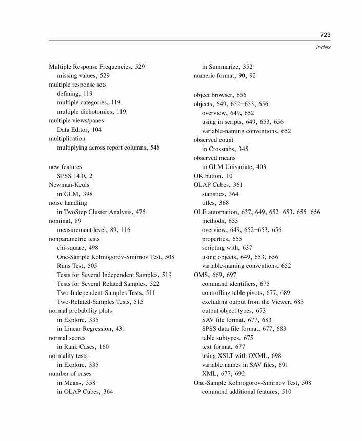
723

Index

Multiple Response Frequencies, 529missing values, 529

multiple response sets

defining, 119multiple categories, 119multiple dichotomies, 119

multiple views/panes

Data Editor, 104multiplication

multiplying across report columns, 548

new features

SPSS 14.0, 2Newman-Keuls

in GLM, 398noise handling

in TwoStep Cluster Analysis, 475nominal, 89

measurement level, 89, 116nonparametric tests

chi-square, 498One-Sample Kolmogorov-Smirnov Test, 508Runs Test, 505Tests for Several Independent Samples, 519Tests for Several Related Samples, 522Two-Independent-Samples Tests, 511Two-Related-Samples Tests, 515

normal probability plots

in Explore, 335in Linear Regression, 431

normal scores

in Rank Cases, 160normality tests

in Explore, 335number of cases

in Means, 358in OLAP Cubes, 364

in Summarize, 352numeric format, 90, 92

object browser, 656objects, 649, 652–653, 656

overview, 649, 652using in scripts, 649, 653, 656variable-naming conventions, 652

observed count

in Crosstabs, 345observed means

in GLM Univariate, 403OK button, 10OLAP Cubes, 361

statistics, 364titles, 368

OLE automation, 637, 649, 652–653, 655–656methods, 655overview, 649, 652–653, 656properties, 655scripting with, 637using objects, 649, 653, 656variable-naming conventions, 652

OMS, 669, 697command identifiers, 675controlling table pivots, 677, 689excluding output from the Viewer, 683output object types, 673SAV file format, 677, 683SPSS data file format, 677, 683table subtypes, 675text format, 677using XSLT with OXML, 698variable names in SAV files, 691XML, 677, 692

One-Sample Kolmogorov-Smirnov Test, 508command additional features, 510

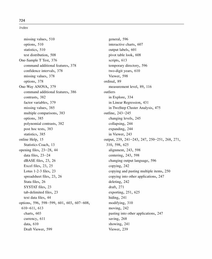
724

Index

missing values, 510options, 510statistics, 510test distribution, 508

One-Sample T Test, 376command additional features, 378confidence intervals, 378missing values, 378options, 378

One-Way ANOVA, 379command additional features, 386contrasts, 382factor variables, 379missing values, 385multiple comparisons, 383options, 385polynomial contrasts, 382post hoc tests, 383statistics, 385

online Help, 15Statistics Coach, 13

opening files, 23–28, 44data files, 23–24dBASE files, 23, 26Excel files, 23, 25Lotus 1-2-3 files, 23spreadsheet files, 23, 26Stata files, 26SYSTAT files, 23tab-delimited files, 23text data files, 44

options, 596, 598–599, 601, 603, 607–608,610–611, 613

charts, 603currency, 611data, 610Draft Viewer, 599

general, 596interactive charts, 607output labels, 601pivot table look, 608scripts, 613temporary directory, 596two-digit years, 610Viewer, 598

ordinal, 89measurement level, 89, 116

outliers

in Explore, 334in Linear Regression, 431in TwoStep Cluster Analysis, 475

outline, 243–245changing levels, 245collapsing, 244expanding, 244in Viewer, 243

output, 239, 241–243, 247, 250–251, 268, 271,310, 598, 625

alignment, 243, 598centering, 243, 598changing output language, 596copying, 242copying and pasting multiple items, 250copying into other applications, 247deleting, 242draft, 271exporting, 251, 625hiding, 241modifying, 310moving, 242pasting into other applications, 247saving, 268showing, 241Viewer, 239

725

Index

Output Management System (OMS), 669, 697output object types

in OMS, 673overview, 701OXML, 698

page control

in column summary reports, 550in row summary reports, 543

page margins, 264page numbering, 264, 267

in column summary reports, 550in row summary reports, 543

page setup, 264–265, 267chart size, 267headers and footers, 265

Paired-Samples T Test, 373missing values, 375options, 375selecting paired variables, 373

pane splitter

Data Editor, 104parallel model

in Reliability Analysis, 553, 555parameter estimates

in GLM Univariate, 403Partial Correlations, 413

command additional features, 416in Linear Regression, 436missing values, 416options, 416statistics, 416zero-order correlations, 416

partial plots

in Linear Regression, 431password protection, 268Paste button, 10

pasting, 249–250charts, 249pivot tables, 249pivot tables as tables, 249special objects, 250

pattern difference measure

in Distances, 421pattern matrix

in Factor Analysis, 457Pearson chi-square

in Crosstabs, 342Pearson correlation


percentage sign, 305in pivot tables, 305

percentages

in Crosstabs, 345percentiles

in Explore, 334in Frequencies, 323

performance, 70caching data, 70

permissions, 82phi

in Crosstabs, 342phi-square distance measure

in Distances, 421PICT files, 251, 257–258, 625

exporting charts, 251, 257–258, 625pie charts

in Frequencies, 325titles, 579

pivot tables, 241, 247–251, 261, 281–286, 290,292–293, 295–297, 299–302, 309–311, 608,625, 631

adding captions, 310

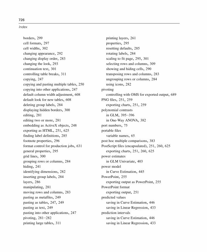
726

Index

borders, 299cell formats, 297cell widths, 302changing appearance, 292changing display order, 283changing the look, 293continuation text, 301controlling table breaks, 311copying, 247copying and pasting multiple tables, 250copying into other applications, 247default column width adjustment, 608default look for new tables, 608deleting group labels, 284displaying hidden borders, 300editing, 281editing two or more, 281embedding as ActiveX objects, 248exporting as HTML, 251, 625finding label definitions, 285footnote properties, 296format control for production jobs, 631general properties, 295grid lines, 300grouping rows or columns, 284hiding, 241identifying dimensions, 282inserting group labels, 284layers, 286manipulating, 281moving rows and columns, 283pasting as metafiles, 249pasting as tables, 247, 249pasting as text, 249pasting into other applications, 247pivoting, 281–282printing large tables, 311

printing layers, 261properties, 295resetting defaults, 285rotating labels, 284scaling to fit page, 295, 301selecting rows and columns, 309showing and hiding cells, 290transposing rows and columns, 283ungrouping rows or columns, 284using icons, 282

pivoting

controlling with OMS for exported output, 689PNG files, 251, 259

exporting charts, 251, 259polynomial contrasts

in GLM, 395–396in One-Way ANOVA, 382

port numbers, 75portable files

variable names, 65post hoc multiple comparisons, 383PostScript files (encapsulated), 251, 260, 625

exporting charts, 251, 260, 625power estimates

in GLM Univariate, 403power model

in Curve Estimation, 445PowerPoint, 255

exporting output as PowerPoint, 255PowerPoint format

exporting output, 251predicted values

saving in Curve Estimation, 446saving in Linear Regression, 433

prediction intervals

saving in Curve Estimation, 446saving in Linear Regression, 433

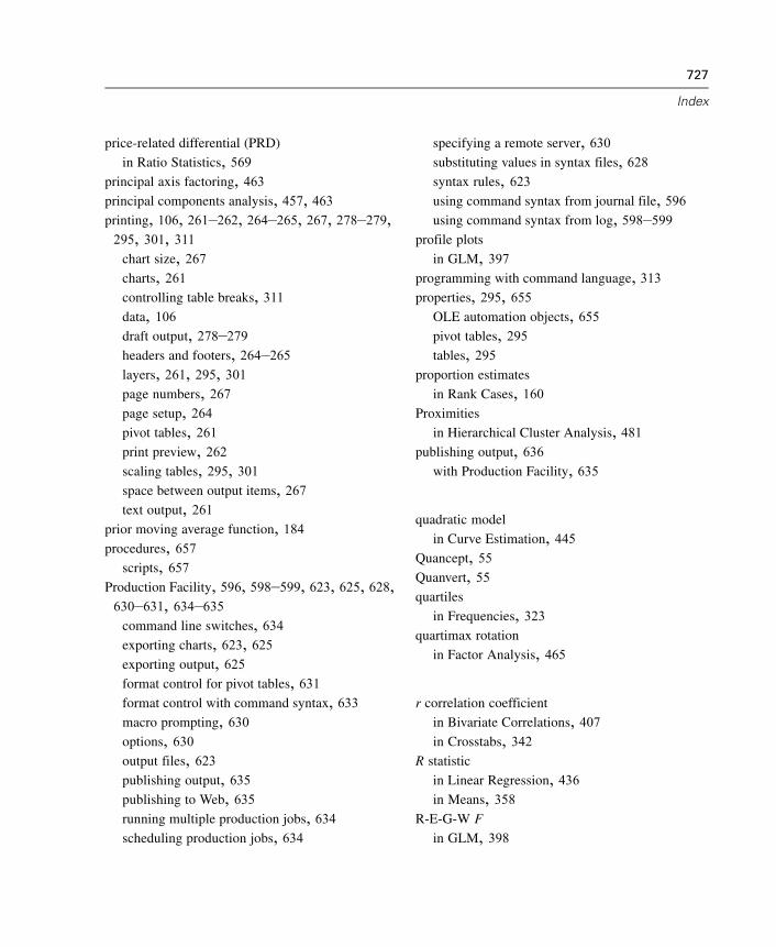
727

Index

price-related differential (PRD)

in Ratio Statistics, 569principal axis factoring, 463principal components analysis, 457, 463printing, 106, 261–262, 264–265, 267, 278–279,

295, 301, 311chart size, 267charts, 261controlling table breaks, 311data, 106draft output, 278–279headers and footers, 264–265layers, 261, 295, 301page numbers, 267page setup, 264pivot tables, 261print preview, 262scaling tables, 295, 301space between output items, 267text output, 261

prior moving average function, 184procedures, 657

scripts, 657Production Facility, 596, 598–599, 623, 625, 628,

630–631, 634–635command line switches, 634exporting charts, 623, 625exporting output, 625format control for pivot tables, 631format control with command syntax, 633macro prompting, 630options, 630output files, 623publishing output, 635publishing to Web, 635running multiple production jobs, 634scheduling production jobs, 634

specifying a remote server, 630substituting values in syntax files, 628syntax rules, 623using command syntax from journal file, 596using command syntax from log, 598–599

profile plots

in GLM, 397programming with command language, 313properties, 295, 655

OLE automation objects, 655pivot tables, 295tables, 295

proportion estimates

in Rank Cases, 160Proximities

in Hierarchical Cluster Analysis, 481publishing output, 636

with Production Facility, 635

quadratic model

in Curve Estimation, 445Quancept, 55Quanvert, 55quartiles

in Frequencies, 323quartimax rotation

in Factor Analysis, 465

r correlation coefficient


R statistic

in Linear Regression, 436in Means, 358

R-E-G-W F

in GLM, 398

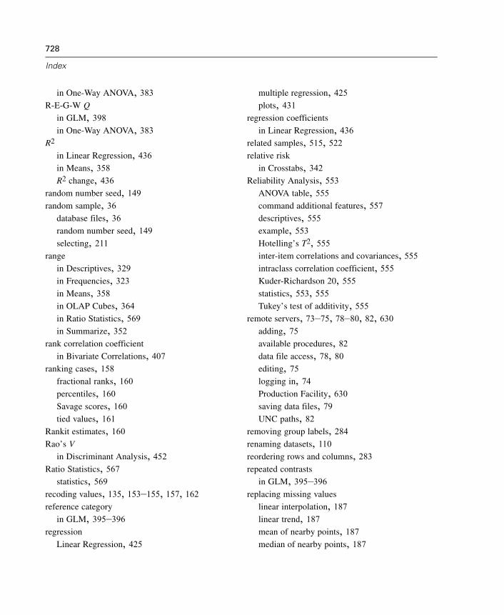
728

Index

in One-Way ANOVA, 383R-E-G-W Q


R2

in Linear Regression, 436in Means, 358R2 change, 436

random number seed, 149random sample, 36

database files, 36random number seed, 149selecting, 211

range

in Descriptives, 329in Frequencies, 323in Means, 358in OLAP Cubes, 364in Ratio Statistics, 569in Summarize, 352

rank correlation coefficient

in Bivariate Correlations, 407ranking cases, 158

fractional ranks, 160percentiles, 160Savage scores, 160tied values, 161

Rankit estimates, 160Rao’s V

in Discriminant Analysis, 452Ratio Statistics, 567

statistics, 569recoding values, 135, 153–155, 157, 162reference category

in GLM, 395–396regression

Linear Regression, 425

multiple regression, 425plots, 431

regression coefficients

in Linear Regression, 436related samples, 515, 522relative risk

in Crosstabs, 342Reliability Analysis, 553

ANOVA table, 555command additional features, 557descriptives, 555example, 553Hotelling’s T2, 555inter-item correlations and covariances, 555intraclass correlation coefficient, 555Kuder-Richardson 20, 555statistics, 553, 555Tukey’s test of additivity, 555

remote servers, 73–75, 78–80, 82, 630adding, 75available procedures, 82data file access, 78, 80editing, 75logging in, 74Production Facility, 630saving data files, 79UNC paths, 82

removing group labels, 284renaming datasets, 110reordering rows and columns, 283repeated contrasts

in GLM, 395–396replacing missing values

linear interpolation, 187linear trend, 187mean of nearby points, 187median of nearby points, 187

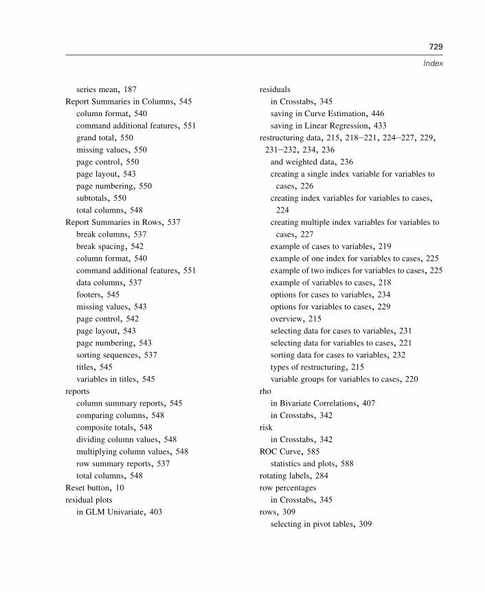
729

Index

series mean, 187Report Summaries in Columns, 545

column format, 540command additional features, 551grand total, 550missing values, 550page control, 550page layout, 543page numbering, 550subtotals, 550total columns, 548

Report Summaries in Rows, 537break columns, 537break spacing, 542column format, 540command additional features, 551data columns, 537footers, 545missing values, 543page control, 542page layout, 543page numbering, 543sorting sequences, 537titles, 545variables in titles, 545

reports

column summary reports, 545comparing columns, 548composite totals, 548dividing column values, 548multiplying column values, 548row summary reports, 537total columns, 548

Reset button, 10residual plots

in GLM Univariate, 403

residuals

in Crosstabs, 345saving in Curve Estimation, 446saving in Linear Regression, 433

restructuring data, 215, 218–221, 224–227, 229,231–232, 234, 236

and weighted data, 236creating a single index variable for variables to

cases, 226creating index variables for variables to cases,

224creating multiple index variables for variables to

cases, 227example of cases to variables, 219example of one index for variables to cases, 225example of two indices for variables to cases, 225example of variables to cases, 218options for cases to variables, 234options for variables to cases, 229overview, 215selecting data for cases to variables, 231selecting data for variables to cases, 221sorting data for cases to variables, 232types of restructuring, 215variable groups for variables to cases, 220

rho


risk

in Crosstabs, 342ROC Curve, 585

statistics and plots, 588rotating labels, 284row percentages

in Crosstabs, 345rows, 309

selecting in pivot tables, 309

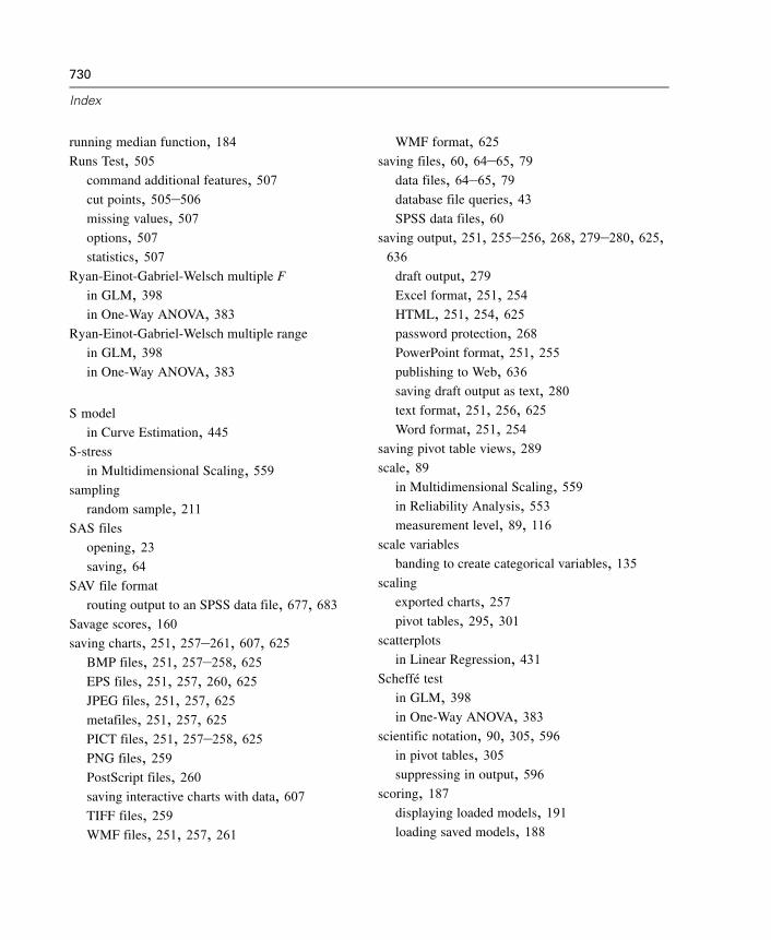
730

Index

running median function, 184Runs Test, 505

command additional features, 507cut points, 505–506missing values, 507options, 507statistics, 507

Ryan-Einot-Gabriel-Welsch multiple F


Ryan-Einot-Gabriel-Welsch multiple range


S model

in Curve Estimation, 445S-stress

in Multidimensional Scaling, 559sampling

random sample, 211SAS files

opening, 23saving, 64

SAV file format

routing output to an SPSS data file, 677, 683Savage scores, 160saving charts, 251, 257–261, 607, 625

BMP files, 251, 257–258, 625EPS files, 251, 257, 260, 625JPEG files, 251, 257, 625metafiles, 251, 257, 625PICT files, 251, 257–258, 625PNG files, 259PostScript files, 260saving interactive charts with data, 607TIFF files, 259WMF files, 251, 257, 261

WMF format, 625saving files, 60, 64–65, 79

data files, 64–65, 79database file queries, 43SPSS data files, 60

saving output, 251, 255–256, 268, 279–280, 625,636

draft output, 279Excel format, 251, 254HTML, 251, 254, 625password protection, 268PowerPoint format, 251, 255publishing to Web, 636saving draft output as text, 280text format, 251, 256, 625Word format, 251, 254

saving pivot table views, 289scale, 89

in Multidimensional Scaling, 559in Reliability Analysis, 553measurement level, 89, 116

scale variables

banding to create categorical variables, 135scaling

exported charts, 257pivot tables, 295, 301

scatterplots

in Linear Regression, 431Scheffé test


scientific notation, 90, 305, 596in pivot tables, 305suppressing in output, 596

scoring, 187displaying loaded models, 191loading saved models, 188

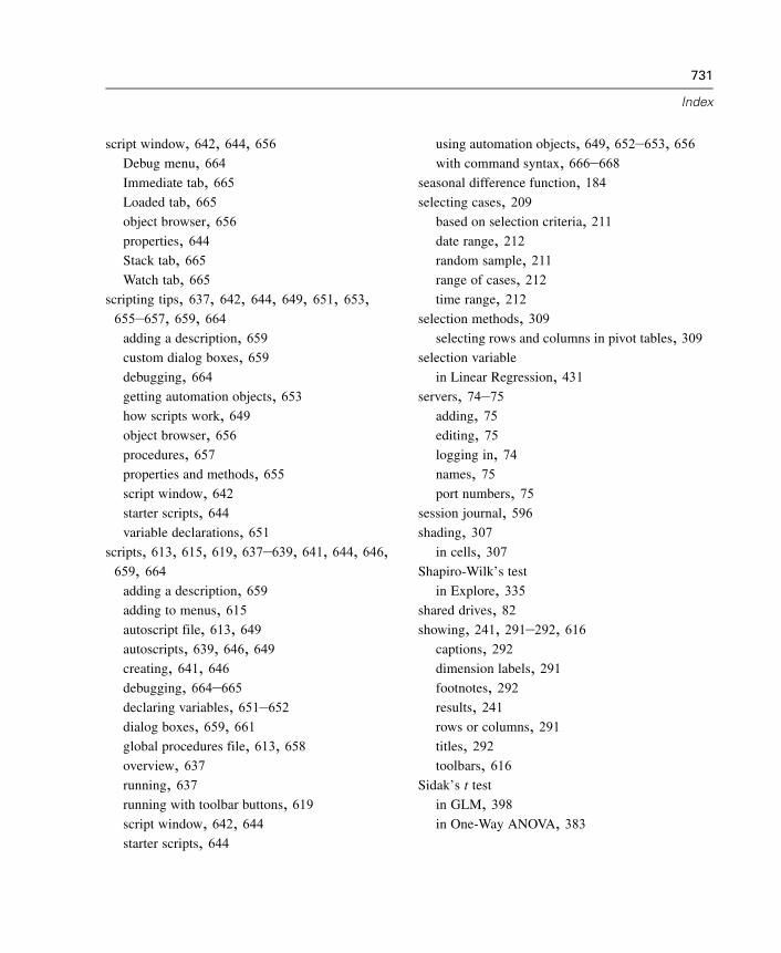
731

Index

script window, 642, 644, 656Debug menu, 664Immediate tab, 665Loaded tab, 665object browser, 656properties, 644Stack tab, 665Watch tab, 665

scripting tips, 637, 642, 644, 649, 651, 653,655–657, 659, 664

adding a description, 659custom dialog boxes, 659debugging, 664getting automation objects, 653how scripts work, 649object browser, 656procedures, 657properties and methods, 655script window, 642starter scripts, 644variable declarations, 651

scripts, 613, 615, 619, 637–639, 641, 644, 646,659, 664

adding a description, 659adding to menus, 615autoscript file, 613, 649autoscripts, 639, 646, 649creating, 641, 646debugging, 664–665declaring variables, 651–652dialog boxes, 659, 661global procedures file, 613, 658overview, 637running, 637running with toolbar buttons, 619script window, 642, 644starter scripts, 644

using automation objects, 649, 652–653, 656with command syntax, 666–668

seasonal difference function, 184selecting cases, 209

based on selection criteria, 211date range, 212random sample, 211range of cases, 212time range, 212

selection methods, 309selecting rows and columns in pivot tables, 309

selection variable

in Linear Regression, 431servers, 74–75

adding, 75editing, 75logging in, 74names, 75port numbers, 75

session journal, 596shading, 307

in cells, 307Shapiro-Wilk’s test

in Explore, 335shared drives, 82showing, 241, 291–292, 616

captions, 292dimension labels, 291footnotes, 292results, 241rows or columns, 291titles, 292toolbars, 616

Sidak’s t test


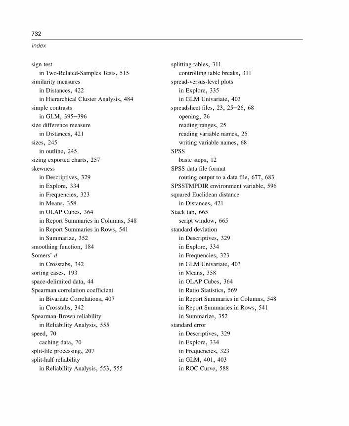
732

Index

sign test

in Two-Related-Samples Tests, 515similarity measures

in Distances, 422in Hierarchical Cluster Analysis, 484

simple contrasts

in GLM, 395–396size difference measure

in Distances, 421sizes, 245

in outline, 245sizing exported charts, 257skewness

in Descriptives, 329in Explore, 334in Frequencies, 323in Means, 358in OLAP Cubes, 364in Report Summaries in Columns, 548in Report Summaries in Rows, 541in Summarize, 352

smoothing function, 184Somers’ d

in Crosstabs, 342sorting cases, 193space-delimited data, 44Spearman correlation coefficient


Spearman-Brown reliability

in Reliability Analysis, 555speed, 70

caching data, 70split-file processing, 207split-half reliability

in Reliability Analysis, 553, 555

splitting tables, 311controlling table breaks, 311

spread-versus-level plots

in Explore, 335in GLM Univariate, 403

spreadsheet files, 23, 25–26, 68opening, 26reading ranges, 25reading variable names, 25writing variable names, 68

SPSS

basic steps, 12SPSS data file format

routing output to a data file, 677, 683SPSSTMPDIR environment variable, 596squared Euclidean distance

in Distances, 421Stack tab, 665

script window, 665standard deviation

in Descriptives, 329in Explore, 334in Frequencies, 323in GLM Univariate, 403in Means, 358in OLAP Cubes, 364in Ratio Statistics, 569in Report Summaries in Columns, 548in Report Summaries in Rows, 541in Summarize, 352

standard error

in Descriptives, 329in Explore, 334in Frequencies, 323in GLM, 401, 403in ROC Curve, 588

733

Index

standard error of kurtosis


standard error of skewness


standard error of the mean


standardization

in TwoStep Cluster Analysis, 475standardized residuals


standardized values

in Descriptives, 327starter scripts, 644Stata files, 26

opening, 26reading, 23saving, 64

Statistics Coach, 13status bar, 8

hiding, 9showing, 9

stem-and-leaf plots

in Explore, 335stepwise selection

in Linear Regression, 430stress

in Multidimensional Scaling, 559strictly parallel model

in Reliability Analysis, 553, 555string format, 90

string variables, 94, 99breaking up long strings in earlier releases, 65computing new string variables, 148entering data, 99in dialog boxes, 9missing values, 94recoding into consecutive integers, 162

Student-Newman-Keuls


Student’s t test, 369Studentized residuals

in Linear Regression, 433subgroup means, 355, 361subroutine procedures, 657subsets of cases

random sample, 211selecting, 209, 211–212

subtitles

in charts, 579subtotals

in column summary reports, 550subtypes, 675

vs. labels, 676sum

in Descriptives, 329in Frequencies, 323in Means, 358in OLAP Cubes, 364in Summarize, 352

sum of squares, 394in GLM, 393

Summarize, 349options, 351statistics, 352

734

Index

syntax, 313, 319, 596, 598–599, 619, 623, 666,668

accessing SPSS Command Syntax Reference, 15journal file, 318, 320, 596log, 598–599output log, 316pasting, 315pasting into scripts, 668Production Facility rules, 623running, 319running command syntax with toolbar buttons,

619syntax rules, 313with scripts, 666–668

SYSTAT files, 23opening, 23

t test

in GLM Univariate, 403in Independent-Samples T Test, 369in One-Sample T Test, 376in Paired-Samples T Test, 373

T4253H smoothing, 184tab-delimited files, 23, 25, 44, 64–65, 68

opening, 23reading variable names, 25saving, 64–65writing variable names, 68

table breaks, 311table subtypes, 675

vs. labels, 676TableLooks, 293–294

applying, 293creating, 294

tables, 311controlling table breaks, 311

Tamhane’s T2


target lists, 593tau-b

in Crosstabs, 342tau-c

in Crosstabs, 342templates, 96–97, 603

in charts, 582, 603using an external data file as a template, 122variable definition, 96–97

temporary active file, 70temporary directory, 596

setting location in local mode, 596SPSSTMPDIR environment variable, 596

temporary disk space, 68, 70tests for independence

chi-square, 342tests for linearity

in Means, 358Tests for Several Independent Samples, 519

command additional features, 522defining range, 521grouping variables, 521missing values, 522options, 522statistics, 522test types, 521

Tests for Several Related Samples, 522command additional features, 525statistics, 525test types, 524

text, 44, 246, 251, 256, 271, 280, 310, 625adding a text file to the Viewer, 246adding to Viewer, 246creating text output, 271

735

Index

data files, 44exporting draft output as text, 280exporting output as text, 251, 256, 625in cells, 310

TIFF files, 259exporting charts, 251, 257, 259, 625

time series analysis

forecast, 446predicting cases, 446

time series data

creating new time series variables, 183data transformations, 180defining date variables, 181replacing missing values, 185transformation functions, 184

titles, 246adding to Viewer, 246in charts, 579in OLAP Cubes, 368

tolerance

in Linear Regression, 436toolbars, 616, 618–620

creating, 616, 619creating new tools, 619customizing, 616, 619displaying in different windows, 618editing bitmap icons, 620showing and hiding, 616

total column

in reports, 548total percentages

in Crosstabs, 345totals, 638

automatically bolding in output, 638transformation matrix

in Factor Analysis, 457transposing rows and columns, 283

transposing variables and cases, 194tree depth

in TwoStep Cluster Analysis, 475trigger events, 648

autoscripts, 648trimmed mean

in Explore, 334Tukey estimates, 160Tukey’s b test


Tukey’s biweight estimator

in Explore, 334Tukey’s honestly significant difference


Tukey’s test of additivity

in Reliability Analysis, 553, 555Two-Independent-Samples Tests, 511

command additional features, 515defining groups, 514grouping variables, 514missing values, 514options, 514statistics, 514test types, 513

Two-Related-Samples Tests, 515command additional features, 519missing values, 518options, 518statistics, 518test types, 517

two-sample t test

in Independent-Samples T Test, 369TwoStep Cluster Analysis, 471

options, 475plots, 477

736

Index

save to external file, 479save to working file, 479statistics, 479

uncertainty coefficient

in Crosstabs, 342unstandardized residuals

in GLM, 401unweighted least squares

in Factor Analysis, 463user-missing values, 94

V

in Crosstabs, 342value labels, 93, 99, 104, 112, 601

applying to multiple variables, 117copying, 117in Data Editor, 104in merged data files, 200in outline pane, 601in pivot tables, 601inserting line breaks, 94using for data entry, 99

values, 305pivot table display format, 305

Van der Waerden estimates, 160variable attributes, 96–97

copying and pasting, 96–97variable declarations, 651–652

in scripts, 651–652naming conventions, 652

variable importance plots

in TwoStep Cluster Analysis, 477variable information, 589variable labels, 92, 596, 601

in dialog boxes, 9, 596

in merged data files, 200in outline pane, 601in pivot tables, 601inserting line breaks, 94

variable lists, 593reordering target lists, 593

variable names, 88, 596generated by OMS, 691in dialog boxes, 9, 596mixed case variable names, 88portable files, 65rules, 88truncating long variable names in earlier releases,

65wrapping long variable names in output, 88

variable pairs, 215creating, 215

variable sets, 591–592defining, 591using, 592

Variable View, 87variables, 11, 88, 102–103, 215, 589, 591, 596

defining, 88defining variable sets, 591definition information, 589display order in dialog boxes, 596in dialog boxes, 9inserting new variables, 102moving, 103recoding, 153–155, 157, 162renaming for merged data files, 199restructuring into cases, 215selecting in dialog boxes, 11variable information in dialog boxes, 12

variance

in Descriptives, 329in Explore, 334

737

Index

in Frequencies, 323in Means, 358in OLAP Cubes, 364in Report Summaries in Columns, 548in Report Summaries in Rows, 541in Summarize, 352

variance inflation factor

in Linear Regression, 436varimax rotation

in Factor Analysis, 465vertical label text, 284Viewer, 239, 241–246, 250, 267–268, 598, 601

changing outline font, 246changing outline levels, 245changing outline sizes, 245collapsing outline, 244copying output, 242deleting output, 242display options, 598displaying data values, 601displaying value labels, 601displaying variable labels, 601displaying variable names, 601excluding output types with OMS, 683expanding outline, 244hiding results, 241moving output, 242outline, 243outline pane, 239pasting special objects, 250results pane, 239saving document, 268space between output items, 267

Wald-Wolfowitz runs

in Two-Independent-Samples Tests, 513

Waller-Duncan t test


Watch tab, 665script window, 665

Web, 636publishing output to, 636

weighted data, 236and restructured data files, 236

weighted least squares

in Linear Regression, 425weighted mean

in Ratio Statistics, 569weighted predicted values

in GLM, 401weighting cases, 213

fractional weights in Crosstabs, 213Welch statistic

in One-Way ANOVA, 385Wilcoxon signed-rank test

in Two-Related-Samples Tests, 515Wilks’ lambda

in Discriminant Analysis, 452window splitter

Data Editor, 104windows, 6

active window, 7designated window, 7

WMF files, 251, 257, 261, 625exporting charts, 251, 257, 261, 625

Word format

exporting output, 251, 254wrapping, 295

controlling column width for wrapped text, 295variable and value labels, 94

738

Index

XML

OXML output from OMS, 698routing output to XML, 677saving output as XML, 669table structure in OXML, 692

XSLT

using with OXML, 698

Yates’ correction for continuity

in Crosstabs, 342years, 610

two-digit values, 610

z scores

in Descriptives, 327in Rank Cases, 160saving as variables, 327

zero-order correlations

in Partial Correlations, 416

SPSS Base 14.0 User’s Guide -...

Documents

Transcript of SPSS Base 14.0 User’s Guide -...