SpringerBriefs in Statistics - unicas.it · material for an introductory course is ... thus...

SpringerBriefs in Statistics

For further volumes:http://www.springer.com/series/8921

Hans-Michael Kaltenbach

A Concise Guide to Statistics

123

Dr. Hans-Michael KaltenbachETH ZurichSchwarzwaldallee 2154002 BaselSwitzerlande-mail: [email protected]

ISSN 2191-544X e-ISSN 2191-5458ISBN 978-3-642-23501-6 e-ISBN 978-3-642-23502-3DOI 10.1007/978-3-642-23502-3Springer Heidelberg Dordrecht London New York

Library of Congress Control Number: 2011937427

� Hans-Michael Kaltenbach 2012This work is subject to copyright. All rights are reserved, whether the whole or part of the material isconcerned, specifically the rights of translation, reprinting, reuse of illustrations, recitation, broadcast-ing, reproduction on microfilm or in any other way, and storage in data banks. Duplication of thispublication or parts thereof is permitted only under the provisions of the German Copyright Law ofSeptember 9, 1965, in its current version, and permission for use must always be obtained fromSpringer. Violations are liable to prosecution under the German Copyright Law.The use of general descriptive names, registered names, trademarks, etc. in this publication does notimply, even in the absence of a specific statement, that such names are exempt from the relevantprotective laws and regulations and therefore free for general use.

Cover design: eStudio Calamar, Berlin/Figueres

Printed on acid-free paper

Springer is part of Springer Science+Business Media (www.springer.com)

To Elke

Preface

This book owes its existence to the lecture ‘‘Statistics for Systems Biology’’, whichI taught in the fall semester 2010 at the Department for Biosystems Science andEngineering of the Swiss Federal Institute of Technology (ETH Zurich). To a largepart, the audience consisted of students with backgrounds in biological sciences,which explains the large proportion of biological examples in this text.

Nevertheless, I hope that this text will be helpful for readers with very differentbackgrounds who need to quantify and analyze data to answer interesting ques-tions. This book is not intended to be a manual, nor can it provide the answer to allquestions and problems that one will encounter when analyzing data. Both thebook title and the title of the book series indicate that space is limited and thisbook therefore concentrates more on the ideas and concepts rather than on pre-senting a vast array of different methods and applications. While all the standardmaterial for an introductory course is covered, this text is very much inspired byLarry Wasserman’s excellent book All of Statistics [1] and consequently discussesseveral topics usually not found in introductory texts, such as the bootstrap, robustestimators, and multiple testing, which are all found in modern statistics software.Due to the space constraints, this book does not cover methods from Bayesianstatistics and does not provide any exercises. Frequent reference is made to thesoftware R (freely available from http://www.r-project.org), but the text itself islargely independent from a particular software.

Should this book provide the reader with enough understanding of the funda-mental concepts of statistics and thereby enable her or him to avoid some pitfallsin the analysis of data and interpretation of the results, such as by providing properconfidence intervals, not ‘‘accepting‘‘ a null hypothesis, or correcting for multipletesting where it is due, I shall be contented.

The book is organized in four chapters: Chapter 1 introduces the basics ofprobability theory, which allows to describe non-deterministic processes and isthus essential for statistics. Chapter 2 covers the inference of parameters andproperties from given data, and introduces various types of estimators, theirproperties, and the computation of confidence intervals to quantify how good agiven estimate is. Robust alternatives to important estimators are also provided.

vii

Chapter 3 is devoted to hypothesis testing, with a main focus on the fundamentalideas and the interpretation of results. This chapter also contains sections on robustmethods and correction for multiple testing, which become more and moreimportant, especially in biology. Finally, Chap. 4 presents linear regression withone and several covariates and one-way analysis-of-variance. This chapter uses Rmore intensively to avoid tedious manual calculations, which the reader hopefullyappreciates.

There surely is no shortage in statistics books. For further reading, I suggest tohave a look at the two books by Wasserman: All of Statistics [1] and All ofNonparametric Statistics [2], which contain a much broader range of topics. Thetwo books by Lehmann, Theory of Point Estimation [3] and Testing StatisticalHypotheses [4] contain almost everything one ever wanted to know about thematerial in Chaps. 2 and 3. For statistics using R, Statistics—An Introduction usingR [5] by Crawley and Introductory Statistics with R [6] by Dalgaard are goodchoices, and The R Book [7] by Crawley offers a monumental reference. The TinyR Handbook [8], published in the same series by Springer, might be a goodcompanion to this book. For statistics related to bioinformatics, Statistical Methodsin Bioinformatics [9] by Ewens and Grant provides lots of relevant information;the DNA sequence example is partly adapted from that book. Finally, for thegerman-speaking audience, I would recommend the two books by Pruscha Stat-istisches Methodenbuch [10], focusing on practical methods, and Vorlesungenüber mathematische Statistik [11], its theory counterpart.

This script was typeset in LATEX, with all except the first two figures and allnumerical data directly generated in R and included using Sweave [12].

I am indebted to many people that allowed this book to enter existence: I thankJörg Stelling for his constant encouragement and support and for enabling me towork on this book. Elmar Hulliger, Ellis Whitehead, Markus Beat Dürr, FabianRudolf, and Robert Gnügge helped correcting various errors and provided manyhelpful suggestions. I thank my fiancée Elke Schlechter for her love and support.Financial support by the EU FP7 project UNICELLSYS is gratefully acknowledged.For all errors and flaws still lurking in the text, the figures, and the examples, I willnevertheless need to take full responsibility.

Basel, July 2011 Hans-Michael Kaltenbach

References

1. Wasserman, L.: All of Statistics. Springer, Heidelberg (2004)2. Wasserman, L.: All of Nonparametric Statistics. Springer, Heidelberg (2006)3. Lehmann, E.L., Casella, G.: Theory of Point Estimation, 2nd edn. Springer, Heidelberg

(1998)4. Lehmann, E.L., Romana, J.P.: Testing Statistical Hypotheses, 3rd edn. Springer, Heidelberg

(2005)5. Crawley, M.J.: Statistics—An Introduction using R. Wiley, New York (2005)

viii Preface

6. Dalgaard, R.: Introductory Statistics with R, 2nd edn. Springer, Heidelberg (2008)7. Crawley, M.J.: The R Book. Wiley, New York (2007)8. Allerhand, M.: A Tiny Handbook of R. Springer, Heidelberg (2011)9. Ewens, W.J., Grant, G.R.: Statistical Methods in Bioinformatics. Springer, Heidelberg (2001)

10. Pruscha, H.: Statistisches Methodenbuch. Springer, Heidelberg (2006)11. Pruscha, H.: Vorlesungen über Mathematische Statistik. Springer, Heidelberg (2000)12. Leisch, F.: Sweave: Dynamic generation of statistical reports. In: Härdle, W., Rönz, B. (eds.)

Compstat 2002—Proceedings in Computational Statistics, pp 575–580 (2002)

Preface ix

Contents

1 Basics of Probability Theory . . . . . . . . . . . . . . . . . . . . . . . . . . . . 11.1 Probability and Events . . . . . . . . . . . . . . . . . . . . . . . . . . . . . . 11.2 Random Variables . . . . . . . . . . . . . . . . . . . . . . . . . . . . . . . . . 81.3 The Normal Distribution . . . . . . . . . . . . . . . . . . . . . . . . . . . . 141.4 Important Distributions and Their Relations . . . . . . . . . . . . . . . 151.5 Quantiles . . . . . . . . . . . . . . . . . . . . . . . . . . . . . . . . . . . . . . . 161.6 Moments . . . . . . . . . . . . . . . . . . . . . . . . . . . . . . . . . . . . . . . 17

1.6.1 Expectation . . . . . . . . . . . . . . . . . . . . . . . . . . . . . . . . 171.6.2 Variance and Standard Deviation . . . . . . . . . . . . . . . . . 181.6.3 Z-Scores. . . . . . . . . . . . . . . . . . . . . . . . . . . . . . . . . . . 201.6.4 Covariance and Independence. . . . . . . . . . . . . . . . . . . . 211.6.5 General Moments; Skewness and Kurtosis . . . . . . . . . . . 22

1.7 Important Limit Theorems . . . . . . . . . . . . . . . . . . . . . . . . . . . 231.8 Visualizing Distributions . . . . . . . . . . . . . . . . . . . . . . . . . . . . 24

1.8.1 Summaries . . . . . . . . . . . . . . . . . . . . . . . . . . . . . . . . . 241.8.2 Plotting Empirical Distributions . . . . . . . . . . . . . . . . . . 241.8.3 Quantile–Quantile Plots . . . . . . . . . . . . . . . . . . . . . . . . 251.8.4 Barplots and Boxplots . . . . . . . . . . . . . . . . . . . . . . . . . 26

1.9 Summary . . . . . . . . . . . . . . . . . . . . . . . . . . . . . . . . . . . . . . . 27

2 Estimation . . . . . . . . . . . . . . . . . . . . . . . . . . . . . . . . . . . . . . . . . . 292.1 Introduction . . . . . . . . . . . . . . . . . . . . . . . . . . . . . . . . . . . . . 292.2 Constructing Estimators . . . . . . . . . . . . . . . . . . . . . . . . . . . . . 32

2.2.1 Maximum-Likelihood . . . . . . . . . . . . . . . . . . . . . . . . . 322.2.2 Least-Squares . . . . . . . . . . . . . . . . . . . . . . . . . . . . . . . 342.2.3 Properties of Estimators . . . . . . . . . . . . . . . . . . . . . . . . 34

2.3 Confidence Intervals . . . . . . . . . . . . . . . . . . . . . . . . . . . . . . . 362.3.1 The Bootstrap. . . . . . . . . . . . . . . . . . . . . . . . . . . . . . . 39

xi

2.4 Robust Estimation . . . . . . . . . . . . . . . . . . . . . . . . . . . . . . . . . 422.4.1 Location: Median and k-Trimmed Mean . . . . . . . . . . . . 432.4.2 Scale: MAD and IQR . . . . . . . . . . . . . . . . . . . . . . . . . 45

2.5 Minimax Estimation and Missing Observations . . . . . . . . . . . . . 462.5.1 Loss and Risk. . . . . . . . . . . . . . . . . . . . . . . . . . . . . . . 462.5.2 Minimax Estimators . . . . . . . . . . . . . . . . . . . . . . . . . . 47

2.6 Fisher-Information and Cramér-Rao Bound. . . . . . . . . . . . . . . . 492.7 Summary . . . . . . . . . . . . . . . . . . . . . . . . . . . . . . . . . . . . . . . 51

3 Hypothesis Testing . . . . . . . . . . . . . . . . . . . . . . . . . . . . . . . . . . . . 533.1 Introduction . . . . . . . . . . . . . . . . . . . . . . . . . . . . . . . . . . . . . 533.2 The General Procedure. . . . . . . . . . . . . . . . . . . . . . . . . . . . . . 563.3 Testing the Mean of Normally Distributed Data . . . . . . . . . . . . 58

3.3.1 Known Variance . . . . . . . . . . . . . . . . . . . . . . . . . . . . . 583.3.2 Unknown Variance: t-Tests . . . . . . . . . . . . . . . . . . . . . 61

3.4 Other Tests . . . . . . . . . . . . . . . . . . . . . . . . . . . . . . . . . . . . . . 643.4.1 Testing Equality of Distributions:

Kolmogorov-Smirnov . . . . . . . . . . . . . . . . . . . . . . . . . 643.4.2 Testing for Normality: Shapiro-Wilks . . . . . . . . . . . . . . 643.4.3 Testing Location: Wilcoxon . . . . . . . . . . . . . . . . . . . . . 653.4.4 Testing Multinomial Probabilities: Pearson’s v2 . . . . . . . 673.4.5 Testing Goodness-of-Fit. . . . . . . . . . . . . . . . . . . . . . . . 68

3.5 Sensitivity and Specificity . . . . . . . . . . . . . . . . . . . . . . . . . . . 693.6 Multiple Testing . . . . . . . . . . . . . . . . . . . . . . . . . . . . . . . . . . 71

3.6.1 Bonferroni-Correction . . . . . . . . . . . . . . . . . . . . . . . . . 723.6.2 False-Discovery-Rate (FDR). . . . . . . . . . . . . . . . . . . . . 72

3.7 Combining Results of Multiple Experiments . . . . . . . . . . . . . . . 743.8 Summary . . . . . . . . . . . . . . . . . . . . . . . . . . . . . . . . . . . . . . . 75Reference . . . . . . . . . . . . . . . . . . . . . . . . . . . . . . . . . . . . . . . . . . . 75

4 Regression . . . . . . . . . . . . . . . . . . . . . . . . . . . . . . . . . . . . . . . . . . 774.1 Introduction . . . . . . . . . . . . . . . . . . . . . . . . . . . . . . . . . . . . . 774.2 Classes of Regression Problems . . . . . . . . . . . . . . . . . . . . . . . 784.3 Linear Regression: One Covariate . . . . . . . . . . . . . . . . . . . . . 79

4.3.1 Problem Statement . . . . . . . . . . . . . . . . . . . . . . . . . . . 794.3.2 Parameter Estimation. . . . . . . . . . . . . . . . . . . . . . . . . . 804.3.3 Checking Assumptions . . . . . . . . . . . . . . . . . . . . . . . . 824.3.4 Linear Regression Using R. . . . . . . . . . . . . . . . . . . . . . 834.3.5 On the ‘‘Linear’’ in Linear Regression. . . . . . . . . . . . . . 84

4.4 Linear Regression: Multiple Covariates . . . . . . . . . . . . . . . . . . 854.4.1 Problem Statement . . . . . . . . . . . . . . . . . . . . . . . . . . . 854.4.2 Parameter Estimation. . . . . . . . . . . . . . . . . . . . . . . . . . 864.4.3 Hypothesis Testing and Model Reduction . . . . . . . . . . . 864.4.4 Outliers . . . . . . . . . . . . . . . . . . . . . . . . . . . . . . . . . . . 93

xii Contents

4.4.5 Robust Regression. . . . . . . . . . . . . . . . . . . . . . . . . . . . 964.5 Analysis-of-Variance . . . . . . . . . . . . . . . . . . . . . . . . . . . . . . . 97

4.5.1 Problem Statement . . . . . . . . . . . . . . . . . . . . . . . . . . . 974.5.2 Parameter Estimation . . . . . . . . . . . . . . . . . . . . . . . . . 994.5.3 Hypothesis Testing . . . . . . . . . . . . . . . . . . . . . . . . . . . 99

4.6 Interpreting Error Bars . . . . . . . . . . . . . . . . . . . . . . . . . . . . . . 1064.7 Summary . . . . . . . . . . . . . . . . . . . . . . . . . . . . . . . . . . . . . . . 108Reference . . . . . . . . . . . . . . . . . . . . . . . . . . . . . . . . . . . . . . . . . . . 108

Index . . . . . . . . . . . . . . . . . . . . . . . . . . . . . . . . . . . . . . . . . . . . . . . . 109

Contents xiii

Chapter 1Basics of Probability Theory

Abstract Statistics deals with the collection and interpretation of data. This chapterlays a foundation that allows to rigorously describe non-deterministic processes andto reason about non-deterministic quantities. The mathematical framework is givenby probability theory, whose objects of interest are random quantities, their descrip-tion and properties.

Keywords Probability · Distribution · Moment · Quantile

The laws of probability. So true in general. So fallacious inparticular

Edward Gibbon

1.1 Probability and Events

In statistics, we are concerned with the collection, analysis, and interpretation ofdata, typically given as a random sample from a large set. We therefore need tolay a foundation in probability theory that allows us to formally represent non-deterministic processes and study their properties.

A first example. Let us consider the following situation: a dice is rolled leadingto any of the numbers {1, . . . , 6} as a possible outcome. With two dice, the possibleoutcomes are described by the set

� = {(i, j)|1 ≤ i, j ≤ 6} ,

of size |�| = 36. The set of outcomes that lead to a sum of at least 10 is then

A = {(4, 6), (6, 4), (5, 5), (5, 6), (6, 5), (6, 6)} ⊂ �,

a set of size 6. A first definition of the probability that we will roll a sum of at least10 is given by counting the number of outcomes that lead to a sum larger or equal

H.-M. Kaltenbach, A Concise Guide to Statistics, SpringerBriefs in Statistics, 1DOI: 10.1007/978-3-642-23502-3_1, © Hans-Michael Kaltenbach 2012

2 1 Basics of Probability Theory

10 and divide it by the number of all possible outcomes:

P(A) = |A||�| = 6

36,

with the intuitive interpretation that 6 out of 36 possible outcomes are of the desiredtype. This definition implicitly assumes that each of the 36 possible outcomes hasthe same chance of occurring.

Any collection of possible outcomes X ⊆ � is called an event; the previousdefinition assigns a probability of P(X) = |X |/|�| to such an event. Events are setsand we can apply the usual operations on them: Let A be as above the event of havinga sum of at least 10. Let us further denote by B the event that both dice show aneven number; thus, B = {(2, 2), (2, 4), (2, 6), (4, 2), (4, 4), (4, 6), (6, 2), (6, 4), (6, 6)}and |B| = 9. The event C of rolling a sum of at least 10 and both dice even is thendescribed by the intersection of the two events:

C = A ∩ B = {(4, 6), (6, 4), (6, 6)},and has probability

P(C) = P(A ∩ B) = 3

36.

Similarly, we can ask for the event of rolling a total of at least ten or both dice even.This event corresponds to the union of A and B, since any of the elements of A or Bwill do:

D := A ∪ B = {(5, 5), (5, 6), (6, 5), (2, 2), (2, 4), (2, 6),

(4, 2), (4, 4), (4, 6), (6, 2), (6, 4), (6, 6)} .

The complement of an event corresponds to all possible outcomes that are notcovered by the event itself. For example, the event of not rolling an even numbersimultaneously on both dice is given by the complement of B, which is

BC = �\B = {(i, j) ∈ �|(i, j) �∈ B},with probability

P

(BC

)= 1 − P(B) = 1 − 9

36= 27

36.

The general case. Let � be the set of all possible outcomes of a particular exper-iment and denote by A, B ⊆ � any pair of events. Then, any function P with theproperties

P(�) = 1, (1.1)

1.1 Probability and Events 3

P(A) ≥ 0, (1.2)

P(A ∪ B) = P(A) + P(B) if A ∩ B = ∅ (1.3)

defines a probability measure or simply a probability that allows to compute theprobability of events. The first requirement (1.1) ensures that � is really the set of allpossible outcomes, so any experiment will lead to an element of �; the probabilitythat something happens should thus be one. The second requirement (1.2) is thatprobabilities are never negative (but the probability of events might be zero). Finally,the third requirement (1.3) gives us the algebraic rule how the probability of combinedevents is computed; importantly, this rule only applies for disjoint sets. Using thealgebra of sets as above, we can immediately derive some additional facts:

P

(AC

)= P(�\A) = 1 − P(A),

P(∅) = 1 − P(�) = 0,

A ⊆ B ⇒ P(A) ≤ P(B).

Importantly, there are multiple ways to define a valid probability measure for anygiven set �, so these three requirements do not specify a unique such measure. Forassigning a probability to discrete events like the ones discussed so far, it is sufficientto specify the probability P({ω}) for each possible outcome ω ∈ � of the experiment.For example, a die is described by its outcomes � = {1, 2, 3, 4, 5, 6}. One possibleprobability measure is P({ω}) = 1/6 for each of the six possible outcomes ω; itdescribes a fair die. Another probability is P({1}) = P({3}) = P({5}) = 1/18,

P({2}) = P({4}) = P({6}) = 2/18, in which case the probability to roll an evennumber is twice the probability to roll an odd one. Both probability measures arevalid, and the particular choice depends on the various assumptions that are madewhen modeling the die and its behavior.

Typically, probability measures are either derived from such assumptions or theyare inferred from observed data. Such inference will be covered in Chap. 2. For morecomplex examples, it might not be straightforward to construct a probability measurethat correctly captures all assumptions.

If the possible outcomes � become a continuous set, describing a length, forexample, it is no longer possible to simply assign a probability to each elementof this set to define a probability measure. This case requires more sophisticatedmathematical machinery and is not covered here. However, the following results areessentially the same for discrete and continuous cases.

Union of events. We still need to delve a little deeper into the computation ofevent probabilities. Note that the probability for a union of events is only the sum ofthe two individual probabilities provided the two events do not overlap and there is no


Fig. 1.1 Venn diagram ofthe sets A and B. To computethe size of the union, the“doubly-counted”intersection A ∩ B has to besubtracted once

outcome that belongs to both events. In the above example of events A (sum largerequal 10) and B (both dice even), this is clearly not the case. Consequently, the sizeof their union D is smaller than the sum of the individual sizes of A and B.

For computing the probability of D from A and B, we can use an inclusion-exclusion argument: The size of D is the size of A plus the size of B, minus the sizeof the intersection A ∩ B. This becomes clear if we draw a Venn-diagram of the setsas in Fig. 1.1. The elements in the intersection are counted twice and we thereforehave to correct by subtracting it once. Indeed,

|D| = |A| + |B| − |A ∩ B|,and thus

P(D) = |A||�| + |B|

|�| − |A ∩ B||�| = P(A) + P(B) − P(A ∩ B).

Note that if A ∩ B = ∅, we recover the case (1.3) given in the original definition.The inclusion–exclusion calculation is also possible for more than two sets, but

does get a little more involved: already for three sets, we now count some subsetstwice and three times.

Independence. One of the most important concepts in probability and statistics isindependence. Two events X and Y are independent if the knowledge that Y alreadyoccurred does not influence the probability that X will occur. In other words, knowingthat Y happened gives us no information on whether X also happened or not, and vice-versa.

As an example, let us again look at rolling two dice: with some justification, wemay assume that the roll of the first die does not influence the roll of the second. Inparticular, it does not matter whether we roll both dice at once or roll the first andthen roll the second. In this example, the independence of the two dice is a modelingassumption and other modeling assumptions are possible.

Formally, two events X and Y are independent if

P(X ∩ Y ) = P(X)P(Y ),

which means that the probability that both X and Y occur is the probability that Xoccurs times the probability that Y occurs.


In the dice example, the event E = {(i, j)|i ≥ 5} of rolling a 5 or 6 on the first die,and F = {(i, j)| j ≥ 5} of rolling a 5 or 6 on the second die, are independent. Indeed,P(E ∩ F) = P({(i, j)|i ≥ 5, j ≥ 5}) = P({(5, 5), (5, 6), (6, 5), (6, 6)}) = 4

36 andP(E) = P(F) = 2

6 .

If two events are not independent, the probability of X happening provided wealready know that Y happened is captured by the conditional probability of X givenY, which we denote by P(X |Y ). This probability is given by

P(X |Y ) = P(X ∩ Y )

P(Y ),

and might be easier to remember in its equivalent form P(X |Y )P(Y ) = P(X ∩ Y ),which reads “the probability of X and Y happening simultaneously is the probabilitythat Y happens times the probability that X happens if Y happened”. For example,what is the probability to roll at least a total of 10, if we already know that both diceare even? There are |B| = 9 possible outcomes that lead to both dice even. Fromthese, |A ∩ B| = 3 have a sum of 10 or greater, leading to the probability

P(A|B) = P(A ∩ B)

P(B)=

3369

36

= 3

9.

If two events X and Y are independent, we have

P(X |Y ) = P(X),

as we would expect. This also agrees with the above interpretation: The probabilityof X happening is the same, irrespective of knowing whether Y happened or not.

The law of total probability states that

P(X) = P(X ∩ Y1) + · · · + P(X ∩ Yn),

where the Yi form a partition of �, i.e., cover all possible outcomes without cover-ing one outcome twice. We can read this as “the probability that X happens is theprobability that X and Y1 happen simultaneously or X and Y2 happen simultaneouslyetc.”. The example in Fig. 1.2 gives an intuitive representation of the theorem.

Together, conditional probabilities and the law of total probability are powerfultools for computing the probability of particular events.

Example 1 Let us consider an urn containing 2 white and 3 black balls, from whichtwo balls are drawn, and are not put back in (this is known as drawing withoutreplacement). Let us denote by C the event that we draw two identical colors, nomatter which one, and by W and B the event of the first ball being white, respectivelyblack. Provided we know the first ball is white, we can conclude that there are 1white and 3 black balls left in the urn. The probability to draw another white ballthus became

P(C |W ) = 1/4.


Fig. 1.2 Law of totalprobability: P(X) =P(X ∩ Y1) + · · · + P(X ∩ Yn)

if the Yi partition �

Similarly, if we know the first ball is black, we can conclude 2 white and 2 blackballs being left and thus

P(C |B) = 2/4.

By the law of total probability, P(C) is the probability to draw another white ball ifwe have a white, times the probability to draw a white in the first place plus the samefor black:

P(C) = P(C ∩ W ) + P(C ∩ B) = P(C |W )P(W ) + P(C |B)P(B).

With P(W ) = 2/5 and P(B) = 3/5 this amounts to P(C) = 2/5.

Bayes’ rule. Bayes’ rule is an important tool for manipulating conditional proba-bilities. It allows us to “invert” conditional probabilities by

P(Y |X) = P(X |Y )P(Y )

P(X), (1.4)

which becomes evident if we simply multiply by P(X) to arrive at P(Y ∩ X) = P(X ∩Y ).The two probabilities for X and Y are called the prior probabilities, as they describethe chance that either event happens without taking into account any informationabout the other event. The left-hand side of (1.4) is called the posterior. Whilealgebraically simple, this rule is very helpful in computing conditional probabilitiesin a variety of situations.

Example 2 Let us consider the following situation: a patient is going to see a doctorfor an annual checkup and in the battery of tests that are performed, the test for aparticular disease D comes back positive. The doctor is concerned, as he read inthe brochure that this particular test has a probability of 0.9 to correctly detect thedisease if the patient actually has it, and also a probability of 0.9 to correctly detectif the patient does not have it. Should the patient be concerned, too?

Let us denote by + and − the events of positive, respectively negative, outcomeof the test. From the brochure information, we know that


P(+|D) = 0.9,

P(−|DC ) = 0.9.

But what we are really interested in is the probability P(D|+) that the patient actuallyhas the disease, provided the test says so. We compute this probability via Bayes’rule as

P(D|+) = P(+|D)P(D)

P(+).

We would therefore need to know the probability P(D) that a patient has the diseasein the first place (regardless of any test results) and the probability P(+) that thetest will be positive (regardless of whether the patient is sick). The latter is easilycomputed using the law of total probability

P(+) = P(+|D)P(D) + P(+|DC )P(DC ),

and

P(+|DC ) = 1 − P(−|DC ).

The only thing we need to figure out is P(D), the probability to be sick in thefirst place. We might imagine this as the probability that, randomly picking someonefrom the street, this person is actually sick. It is important to understand that thisprobability has to be provided from the outside, as it cannot be derived from theinformation available in the problem specification. In our case, such data might beavailable from public health institutions. Let us assume that 1 in 100 people are sick,so P(D) = 0.01 and consequently

P(+) = 0.9 × 0.01 + (1 − 0.9) × (1 − 0.01) = 0.108,

that is, for about one out of ten people, the test will be positive, irrespective of theiractual health. This is simply because few people have the disease, but in one outof ten, the test will be incorrect. We assembled all information needed to actuallycompute the relevant probability:

P(D|+) = 0.9 × 0.01

0.108≈ 0.08.

Maybe surprisingly, the probability to have the disease if the test is positive is lessthat 10% and getting a second opinion is clearly indicated! This is one reason toperform a second independent test in such a case.

The key point of this example is to not get confused by the two conditionalprobabilities P(X |Y ) and P(Y |X) and mistakenly assume them to be equal or atleast of comparable size. As shown, the two can be very different, depending on theprior probabilities for X and Y.


Implications of Bayes’ rule. Bayes’ rule has some more implications along theselines, which we will briefly describe in a very informal manner: As we will see inthe chapter on statistical hypothesis testing, classical techniques only allow us tocompute the probability of seeing certain data D (e.g., a measurement), provided agiven hypothesis H is true; very informally, P(D|H). Of course, we actually want toknow the probability P(H |D) of the hypothesis being true, given the data. However,Bayes’ rule shows that this probability can only be computed if we have informationabout the hypothesis being true irrespective of any data. Again, this informationabout prior probabilities has to come from “outside” and cannot be inferred from thehypothesis or the data. Typically, this information is provided by either additionalassumptions or by looking into other data. The branch of Bayesian Statistics dealswith the incorporation of such prior data and provides many alternative ways ofinference and hypothesis testing. However, many of these methods are more elaborateand special care needs to be taken to correctly apply them, which is one reason whywe do not cover them in this text.

1.2 Random Variables

While events and algebraic set operations form the basis for describing random exper-iments, we gain much more flexibility and widen the applications of probability byintroducing random variables. Technically, these are functions mapping an outcomeω ∈ � to a number. For example, we can describe the two dice example simply bydefining the number of eyes rolled with die i as the random variable Xi . The eventof having at least a 5 on the first die is then described intuitively by the statementX1 ≥ 5. Similarly, we can formulate the event that the sum is larger than 10 byX1 + X2 ≥ 10, instead of listing all corresponding outcomes.

Once probabilities are assigned to events, they transfer to random variables simplyby finding the corresponding event described by a statement on the random variables.Formally, P(X ∈ X ) = P({ω|X (ω) ∈ X }).

For the two dice example, let us compute the probability of rolling at least a 5with the first die using the random variable X1:

P(X1 ≥ 5) = P (X1 ∈ {5, 6}) = P ({ω ∈ �|X1(ω) ∈ {5, 6}})= P({(i, j)|i ≥ 5, 1 ≤ j ≤ 6})= P({(i, j)|i = 5}) + P({(i, j)|i = 6}) = 12

36.

The joint probability of two random variables X and Y simultaneously takingvalues in their respective sets is given by the intersection of the corresponding events:

P(X ∈ X , Y ∈ Y ) = P ({ω|X (ω) ∈ X } ∩ {ω|Y (ω) ∈ Y }) .

1.2 Random Variables 9

The advantage of working with random variables instead of events comes from thefact that random variables have a probability distribution that describes the proba-bility that the random variable takes a value smaller or equal to a certain number.The cumulative distribution function (cdf) FX () of a random variable X is defined asFX (x) = P(X ≤ x). It always starts with a value of 0 at x = −∞ and monotonicallyincreases to 1 for larger values of x. Often, very different problems lead to the samedistribution for the involved random variables, which is why some distributions gettheir own name and their properties can be found in tables.

Similar to events, random variables also come in two distinct flavors: they eithertake values in a discrete (but maybe infinite) set of values, as in the dice example, orthey take values from a continuous set, like the set of real numbers RI.

Discrete Random Variables. A discrete random variable A has a probability massfunction (pmf) in addition to its cumulative distribution function. The pmf is givenby pA(a) = P(A = a) and we can easily compute the cdf from it by summation:FA(k) = ∑k

a=−∞ pA(a).

Example 3 Let us consider the following experiment: a coin is flipped n times. Theprobability of any flip to show head is given by our first distribution with its ownname: the Bernoulli distribution, which assigns a probability of p to head and 1− p totail. If Xi is the outcome of the ith flip, with Xi = 0 for tail and Xi = 1 for head, thisdistribution is completely described by p, as P(Xi = 0) = 1 − p, P(Xi = 1) = pand P(Xi = k) = 0 for any value k that is neither 0 nor 1. Thus, knowing thatXi is Bernoulli distributed with parameter p completely specifies all we need toknow. In short, this statement is written as X ∼ Bernoulli(p), where “∼” is read as“distributed as”.

What is the probability that we have to wait until the wth flip to see head for thefirst time? This is the question for the distribution of a waiting time W. Let us see: tosee the first head at flip w, all preceding w − 1 flips are necessarily tails. Assumingthe flips to be independent, this probability is

P(X1 = 0, . . . , Xw−1 = 0) = P(X1 = 0) · · · P(Xw−1 = 0) = (1 − p)w−1.

The probability to actually see head in the wth flip is P(Xw = 1) = p. Thus, P(W =w) = (1 − p)w−1 p, the pmf of a geometric distribution, denoted W ∼ Geom(p).

The particular value w is called a realization of the random variable W. This is anexample of a discrete random variable that has infinitely many possible values withpositive probability. The probability mass function of a geometric distribution isgiven in Fig. 1.3 (left).

What is the probability to see exactly h heads if we flip n times? This question is alittle more tricky: the probability to see h heads in n flips is ph . The probability thatthe remaining n−h flips are all tails is (1− p)n−h . But there are a multitude of ways to

arrange the h heads and n−h tails. To be exact, there are( n

h

):= n!

(n−h)!h! (a binomial

coefficient, read “n choose h”) many ways to do so: n! := 1 × 2 × 3 × · · · × n is thenumber of ways to arrange n flips in different order. The h heads can be drawn in h!


2 4 6 8 10

0.00

0.10

0.20

Waiting time

Pro

babi

lity

2 4 6 8 10

0.00

0.10

0.20

Number of heads

Pro

babi

lity

Fig. 1.3 Geometric distribution for p = 0.3 (left) and binomial distribution with n = 10 andp = 0.3 (right)

different orders, which we do not distinguish and treat as equivalent. Similarly, thereare (n − h)! ways to arrange the tails are equivalent, leading to the stated coefficient.More generally, the binomial coefficient gives the number of different ways to drawh objects out of n, if we do not care for the order in which they are drawn. For n = 3,

there are

(32

)= 3 ways to draw exactly two of them: from the set {a, b, c}, the 3

ways are {a, b}, {b, c}, {a, c}. The first set contains two possible ways to draw: firstthe a, then the b, or vice-versa, and similarly for the other two sets.

For our problem, let H be the number of heads in n flips. This is a random variabletaking values between 0 and n. It has a binomial distribution with two parameters nand p and probabilities given by the mass function

P(H = h) =(

nh

)(1 − p)n−h ph;

denoted by H ∼ Binom(n, p). A plot of a binomial probability mass function isgiven in Fig. 1.3 (right).

Let us combine these two calculations of the waiting time and the number of headsby solving the following problem: again, a coin is flipped n times, the probability tosee head is p. Let again H be the number of heads in these n flips and let W be thewaiting time for the first head to appear. For completeness, we set W = n + 1, if nohead appears at all.

What is the probability to simultaneously see h heads with the first head appearingat the wth flip? This questions asks for the joint probability distribution given byP(H = h, W = w).

The two random variables H, W are not independent: if they were, we would haveP(H = h|W = w) = P(H = h). But if no head has appeared at all (so W = n + 1),then the probability to see any more than zero heads, given this information, is zero:P(H = 1|W = n +1) = 0, but P(H = 1) > 0. For working out the correct answer,we therefore need to take this dependency into account. It is always a good idea tocheck some boundary cases first: as we saw,


Table 1.1 Joint probability distribution of (H, W )

w = 1 w = 2 w = 3 w = 4

h = 0 0.000 0.000 0.000 0.125h = 1 0.125 0.125 0.125 0.000h = 2 0.250 0.125 0.000 0.000h = 3 0.125 0.000 0.000 0.000

P(H = 0, W = n +1) = P(H = 0|W = n +1)P(W = n +1) = 1×(1− p)n,

the probability to see n tails. Further, P(H = 0, W = w) = 0 for any w ≤ n, as wecannot have seen the first head somewhere in the sequence if we saw none at all.

What about the non-boundary cases? For (H = h, W = w), we can use thefollowing argument: to see h heads in total, given the first one in the wth flip, weknow that the first w − 1 flips are all tails and we need to place h − 1 heads in theremaining n − w positions (the first is already placed in position w):

P(H = h|W = w) =(

n − wh − 1

)(1 − p)(n−w)−(h−1) ph−1,

the binomial probability of having h −1 heads in n −w trials. The probability of firsthead at w ≤ n is the geometric distribution P(W = w) = (1− p)w−1 p. Combining:

P(H = h, W = w) =(

n − wh − 1

)(1 − p)n−h ph .

The conditional distribution of waiting w flips, given we have h heads in total, iseasily calculated as

P(W = w|H = h) =

(n − wh − 1

)

(nh

) ,

the number of ways to place h − 1 heads in n − w positions over the number ofways to place h heads in n positions. Interestingly, this probability is independentof the probability p to see head. For n = 3 and p = 0.5, the full joint probabilityP(H = h, W = w) is given in Table 1.1.

We might also be interested in computing the waiting time distribution with-out referring to the number of heads. This marginal distribution can be derived byapplying the law of total probability. For example,

P(W = 2) =3∑

h=0

P(H = h, W = 2) = (1 − p)p = 1

4

is the marginal probability that we see the first head in the second flip.


Example 4 To contribute another example, let us consider the following problem,encountered in molecular biology: DNA molecules carrying the inheritance infor-mation of an organism can be modeled as a sequence of nucleotides. There are fourdifferent such nucleotides: arginine (abbreviated A), cytosine (C), guanine (G), andtyrosine (T). A common problem is to determine how closely related two DNAsequences are. To make things easier, let us assume both sequences have the samelength n, that the nucleotides in any two positions in the sequence are independent,and that each nucleotide has a probability of 1/4 to occur in any position. Similarityof the sequences can then be established by counting in how many positions the twosequences have the same nucleotide. Each such case is called a match, the converse amismatch, so the following two sequences have seven matches and three mismatches(underlined):

A C C G T T G G T AA C G G T T C G A A

If the two sequences have nothing in common, we would expect to see a match inabout 1/4 of the cases, and the number of matches would follow a Binom(n, p = 1/4)

distribution. Conversely, evolutionarily related DNA sequences would show a muchhigher proportion of matches.

In subsequent chapters, we will estimate the nucleotide frequencies p from dataand test the hypothesis that sequences are related by comparing the observed andexpected number of matches

Continuous Random Variables. We also need random variables that take valuesin a continuous set to describe, e.g., measured lengths or optical densities. Similar toevents, we cannot cover these in all mathematical rigor. A nontrivial mathematicalargument shows that for such a continuous random variables X, a probability massfunction cannot be defined properly, because P(X = x) = 0 for all x. Instead, mostof these variables have a probability density function (pdf) f X (x) with the properties

fX (x) ≥ 0 ,

∞∫

−∞fX (y)dy = 1.

The density is a function such that the probability of X to take a value in any interval[xl , xu] is given by the area under the density function on this interval, that is, P(xl ≤X ≤ xu) = ∫ xu

xlfX (y)dy. This probability can also be written in terms of the

cumulative distribution function

FX (x) = P(X ≤ x) =x∫

−∞fX (y)dy


Fig. 1.4 Density of Exp(λ)

distribution for λ = 2. Thegray shaded area gives theprobability of W falling inthe range [0.5, 2]

0 1 2 3 4

0.0

1.0

2.0

w

Exp

. den

sity

as the difference FX (xu) − FX (xl). Important continuous distributions include theexponential (see Ex. 5 below) and the normal distributions (covered in Sect. 1.3). InSect. 1.4, we will discuss several more distributions that frequently arise in statistics,like the t-, the χ2- and the F-distributions, and also demonstrate various relationsbetween them.

Example 5 As a first example for a continuous random variable, let us consider theexponential distribution. This distribution often describes the waiting time W for anevent such as a radioactive decay and has density function

fW (w; λ) = λ exp(−λw),

where the rate λ > 0 is the distribution’s only parameter and 1/λ describes theaverage waiting time for the next event. The cumulative distribution function iseasily calculated as

FW (w; λ) = 1 − exp(−λw).

Figure 1.4 shows the density function for λ = 2, the area of the gray region givesthe probability that a random variable W ∼ Exp(2) takes a value between 0.5 and 2,which we calulate to be

P(0.5 ≤ W ≤ 2) =2∫

0.5

2 × exp(−2 × w)dw = 0.3496.

Example 6 Another example for a continuous distribution is the uniform distribution,which has the same density for each point in a certain interval. If U ∼ Unif([a, b]),the density is given by

fU (u) ={ 1

b−a , if a ≤ u ≤ b,

0, else.

It is important to understand that the probability density values cannot be inter-preted as probabilities. In particular

fX (x) �≤ 1.


−4 −2 0 2 4 6 8

0.0

0.1

0.2

0.3

0.4

Value

Nor

mal

den

sity

−4 −2 0 2 4 6 8

0.0

0.2

0.4

0.6

0.8

1.0

Value

CD

F

Fig. 1.5 Density functions (left) and cumulative distribution functions (right) of Norm(μ, σ 2) dis-tribution with parameters (0, 1) (solid), (0, 3) (dashed), and (3, 3) (dotted)

As an easy counterexample, let us consider a uniform random variable U on aninterval [a, b]. For the interval [a, b] = [0, 0.5], the density function is fU (u) = 2for each value u inside the interval. Moreover, by moving the right boundary b ofthe interval towards a, we can make fU (u) arbitrarily large. Thus, it clearly cannotbe interpreted as a probability. The integral of the density over any subinterval is ofcourse still a probability.

1.3 The Normal Distribution

Probably the best known continuous distribution is the normal distribution, some-times also called the Gaussian distribution, as it was first completely described byC. F. Gauß. This distribution has two parameters, μ and σ 2. Its probability densityfunction is

f (x;μ, σ 2) = 1√2πσ 2

e− (x−μ)2

2σ2 .

The normal density function has the famous bell-shaped curve and is symmetricaround μ; its “width” is determined by σ. Figure 1.5 (left) shows the density of threenormal distributions with parameters (μ, σ 2) = (0, 1), (0, 3), and (3, 3), respectively.The corresponding cumulative distribution functions are given in Fig. 1.5 (right).

The normal distribution is so important in probability theory and statistics, that itsdensity and cumulative distribution functions even have their own letters reserved forthem: φ(x;μ, σ 2) for the pdf and (x;μ, σ 2) for the cdf. If no parameters are given,the two functions refer to the standard normal distribution with μ = 0 and σ = 1.

One of the helpful properties of the normal distribution is that whenever wescale a normal random variable X by multiplying with a fixed a and then shift itby some fixed value b to the new random variable Y = aX + b, this new randomvariable is also normally distributed: with X ∼ Norm(μ, σ 2), we have that Y ∼

1.3 The Normal Distribution 15

Norm(aμ + b, a2σ 2). In particular, for X ∼ Norm(μX , σ 2X ),

Z = X − μX

σX∼ Norm(0, 1)

has a standard normal distribution.Moreover, the sum of random variables with the same, arbitrary distribution does

in general not have the same distribution as the variables themselves. In contrast,adding independent normal random variables always leads to a new normal randomvariable. Let X1 ∼ Norm(μ1, σ

21 ) and X2 ∼ Norm(μ2, σ

22 ) be two independent

normal variables, potentially with different parameters. Then,

X1 + X2 ∼ Norm(μ1 + μ2, σ21 + σ 2

2 ).

1.4 Important Distributions and Their Relations

We will later consider many more distributions that occur in various statistical con-texts. In this section, we briefly review some of these and show how they are relatedamong each other. This will later allow us to more easily understand how manydistributions of estimators and test statistics are derived.

Arguably the most frequently encountered distributions in statistics are those inthe following list:

• Normal distribution, with parameters μ and σ 2,• Student’s t-distribution, with parameter d, the degrees of freedom,• χ2-distribution, with parameter d, the degrees of freedom,• F-distribution, with parameters m, n, two degrees of freedom.

Instead of listing their density functions and properties here, we refer to the fact thatthey are easily available in any statistics package. In R, their distribution functionsare accessible via the functions pnorm, pt, pchisq, and pf, respectively, wherep can be replaced by d,q,r to get the density and quantile functions, or a randomnumber generator, respectively.

These distributions are related as follows.

• X ∼ Norm(μ, σ 2) ⇒ X−μσ

∼ Norm(0, 1).

• Z1, . . . , Zn ∼ Norm(0, 1) ⇒ ∑ni=1 Z2

i ∼ χ2(n), if the Zi are independent.

• X1 ∼ χ2(n), X2 ∼ χ2(m) ⇒ 1n X11m X2

∼ F(n, m), if X1, X2 are independent.

• Z ∼ Norm(0, 1), X ∼ χ2(n) ⇒ Z√1n X

∼ t (n).

• X ∼ t (m) ⇒ X2 ∼ F(1, m).

• X1 ∼ χ2(n), X2 ∼ χ2(m) ⇒ X1 + X2 ∼ χ2(n +m), if X1, X2 are independent.• Xn ∼ t (n) ⇒ limn→∞ Xn ∼ Norm(0, 1).


Fig. 1.6 Standard normaldensity (solid) andt (n)-densities for n = 2(dashed) and n = 20 (dotted)

−4 −2 0 2 4

0.0

0.2

0.4

Value

Den

sity

As an example, let us consider normally distributed random variables Xi and Yi withparameters μX and μY , respectively, and σX = σY = 1. Let us further define thenew random variables VX = ∑n

i=1(Xi − μX )2 and VY = ∑mi=1(Yi − μY )2. These

will later be called variations, as they measure how “spread out” the values of Xand Y are. Both VX and VY are sums of squares of random variables with standardnormal distribution. Thus, both VX and VY follow χ2-distributions with parametersn and m, respectively. Further, their quotient VX/VY is used in regression analysis;we immediately see that it is a quotient of two χ2-variables and therefore has anF(n, m)-distribution if scaled appropriately.

Of particular importance is Student’s t-distribution, which is the quotient of astandard normal random variable and a scaled χ2-variable. For n − 1 degrees offreedom, the t (n − 1)-distribution has density

f (t; n) = (n+1

2

)

√nπ n

2

(1 + t2

n

) n+12

.

The densities of this distribution, with n = 2 and n = 20 degrees of freedom,are given in Fig. 1.6 together with the standard normal density. With increasing n,the t-distribution approaches the standard normal as claimed, but has substantiallyheavier tails for few degrees of freedom.

1.5 Quantiles

While the cumulative distribution function FX (x) describes the probability of arandom variable X to take a value below a certain value x, the quantiles describethe converse: the α-quantile is the value x such that FX (x) = α, i.e., the valuefor which the random variable has a probability of α to take that or a lower value.Slight difficulties might arise if there is not an exact value x but a whole interval,but the interpretation remains the same. The quantile function is then (neglectingtechnicalities) given by F−1

X (α), the inverse function of the cdf. Thus, if P(X ≤q) = α, then q is the α-quantile of X.

1.5 Quantiles 17

−4 −2 0 2 4

0.0

0.1

0.2

0.3

0.4

x

Sta

ndar

d no

rmal

pdf

−4 −2 0 2 4

0.0

0.1

0.2

0.3

0.4

x

Sta

ndar

d no

rmal

pdf

Fig. 1.7 Density of standard normal distribution with 0.05-quantile (left) and 0.8-quantile (right).The gray areas therefore correspond to probabilities of 0.05 and 0.8, respectively

The 0.05- and the 0.8-quantile of a standard normal distribution are given inFig. 1.7 (left and right, respectively) as vertical dashed lines. The α-quantile of thestandard normal distribution is denoted by zα, thus z0.05 = −1(0.05) ≈ −1.645 andz0.8 = −1(0.8) ≈ 0.842. Using the symmetry of the standard normal distribution,z1−α = −zα.

1.6 Moments

While the distribution of a random variable is completely described by the cumulativedistribution function or the density/mass function, it is often helpful to describe itsmain properties by just a few key numbers. Of particular interest are the expectationand the variance.

1.6.1 Expectation

The expectation, expected value, or mean is the number

E(X) :=∞∫

−∞x f (x)dx

for a continuous, and

E(X) :=∞∑

k=−∞kP(X = k)


for a discrete random variable X. The expectation describes the location of the dis-tribution, which informally is the center value around which the possible values ofX disperse; it is often denoted by the letter μ. The expectation behaves nicely whensumming random variables or multiplying them with constants. For random variablesX, Y and a non-random number a we have:

E(X + Y ) = E(X) + E(Y ),

E(aX) = aE(X),

E(XY ) = E(X)E(Y ) if X,Y are independent.

1.6.2 Variance and Standard Deviation

The variance of a random variable X describes how much its values disperse aroundthe expected value and is a measure for the width of its distribution. It is defined as

Var(X) := E((X − E(X))2),

the mean squared distance of values to the expected value and is often denoted byσ 2. A short calculation gives the alternative description

Var(X) = E(X2) − (E(X))2 .

The variance is not linear and we have the following relations for random variablesX, Y and non-random numbers a, b:

Var(X + Y ) = Var(X) + Var(Y ) if X,Y are independent,

Var(X + b) = Var(X),

Var(aX) = a2Var(X).

The square-root σ is called the standard deviation. While it does not contain anymore information than the variance, it is often more convenient for applications, asit is easier to interpret and has the same physical units as the random variable itself.It is a measure for the scale of a distribution, as rescaling X by any factor a changesthe standard deviation by the same factor.

Expectation and variance completely specify a normal distribution, whose twoparameters they are. For X ∼ Norm(μ, σ 2), the following approximations are oftenuseful: the probability of X taking a value x at most one standard deviation awayfrom the mean, i.e., x ∈ [μ− σ,μ+ σ ], is roughly 70%. Similarly, the probabilitiesof observing a value at most 2, respectively 3 standard deviations from the mean,are roughly 95% and 99%, respectively. Note that these probabilities can be verydifferent for non-normal random variables.

1.6 Moments 19

Fig. 1.8 Gamma (solid) andnormal (dashed) densitiesboth with mean μ = 4 andvariance σ 2 = 8,

corresponding to Gammaparameters k = 2 and θ = 2

0 5 10

0.00

0.05

0.10

0.15

x

Den

sity

Example 7 For introducing yet another continuous distribution on the go, let usconsider the Gamma distribution with shape parameter k and scale parameter θ.

It has density function f (x; k, θ) = xk−1 exp(−x/θ)/θk(k), is only defined forx > 0, and describes the distribution of the sum of k exponentially distributedwaiting times, each with rate parameter θ (thus the time to wait for the kth event).This density function is usually not symmetric. For k = 2 and θ = 2, the distributionhas expectation μ = kθ = 4 and variance σ 2 = kθ2 = 8; its density is shown inFig. 1.8 (solid line). For comparison, a normal distribution with the same expectationand variance is plotted by a dashed line. As we can see, the density functions lookvery different, although both have the same mean and variance. For additionallycapturing their different shapes, higher moments are needed (see Sect. 1.6.5).

Example 8 Let us consider the following model of a random DNA sequence as intro-duced earlier: we assume independence among the nucleotides and in each position,the probabilities of having a particular nucleotide are pA, pC , pG , pT , respectively.We investigate two sequences of length n by comparing the nucleotides in the sameposition. Assume that the sequences are completely random and unrelated. At anyposition, the probability of a match is then p := p2

A + p2C + p2

G + p2T , as both

nucleotides have to be the same. Let us set Mi = 1 if the sequences match in posi-tion i and Mi = 0 else.

To decide whether two given sequences are related, we compute the number ofmatching nucleotides and compare it to the number of matches we expect just bychance. If the observed number is much higher than the expected number, we claimthat the sequences are in fact related.1

The total number of matches in two random sequences of length n is given byM := M1 + · · · + Mn and follows a binomial distribution: M ∼ Binom(n, p).

Applying the linearity of the expectation and some algebra, we compute the expectednumber of matches:

1 As a word of caution for the biological audience: this argument does not hold for alignedsequences, as the alignment maximizes the number of matches, and this maximum has a differentdistribution.


E(M) =∞∑

k=−∞kP(M = k)

=n∑

k=0

k

(nk

)pk(1 − p)n−k

=n∑

k=1

np(n − 1)!

(k − 1)!((n − 1) − (k − 1))! pk−1(1 − p)(n−1)−(k−1)

= npn∑

k=1

(n − 1k − 1

)pk−1(1 − p)(n−1)−(k−1)

= np,

where the last equality holds because we have the pmf of a Binom (n −1, p) variablein the sum, which sums to one. The result also makes intuitive sense: the expectednumber of matches is the proportion p of matches times the number of nucleotides n.Consequently, for sequences of length n = 100, with nucleotide probabilities allequal to 0.25, the probability of a match is p = 0.25 and we expect to see 25matches just by chance if the sequences are unrelated.

How surprised are we if we observe 29 matches? Would this give us reason toconclude that the sequences might in fact be related? To answer these questions, wewould need to know how likely it is to see a deviation of 4 from the expected value.This information is captured by the variance, which we can calculate as

Var(M) = Var(M1) + · · · + Var(Mn),

because we assumed that the nucleotides are independent among positions. Usingthe definition of the variance,

Var(M1) = E((M1)2)−(E(M1))

2 = (02 ×(1− p)+12 × p)− p2 = p(1− p),

and we immediately get

Var(M) = nVar(M1) = np(1 − p) = 18.75

and a standard deviation of 4.33 These values indicate that the deviation of theobserved number of matches (=29) from the expected number of matches (=25)is within the range that we would expect to see in unrelated sequences, giving noevidence of the sequences being related. We will see in Chap. 3 how these argumentscan be used for a more rigorous analysis.

1.6.3 Z-Scores

Using the expectation and variance of any random variable X, we can also computea normalized version Z with expectation zero and variance one by

1.6 Moments 21

Z = X − E(X)√Var(X)

.

This random variable is sometimes called the Z-score. For a given realization x ofX, the associated value z of Z tells us how many standard deviations σ the value xis away from its expected value. In essence, this rescales to units of one standarddeviation.

Importantly, however, the distribution of Z might not belong to the same familyas the distribution of X. An important exception is the normal distribution, whereZ ∼ Norm(0, 1) if X ∼ Norm(μ, σ 2).

1.6.4 Covariance and Independence

For two random variables X and Y, we can compute the covariance

Cov(X, Y ) = E ((X − E(X))(Y − E(Y )) ,

to measure how much the variable X varies together with the variable Y (and vice-versa). With this information, we can also calculate the variance of dependent vari-ables by

Var(X + Y ) = Var(X) + Var(Y ) + 2Cov(X, Y ).

As a special case, Cov(X, X) = Var(X). For independent X and Y, the covarianceis zero. The converse, however, is not true, as the following counterexample demon-strates.

Example 9 Let us consider possible outcomes � = {1, 2, 3, 4} and a probabilitymeasure given by P({1}) = P({2}) = 2

5 and P({3}) = P({4}) = 110 . Let us further

define the two random variables X and Y by

ω 1 2 3 4X 1 −1 2 −2Y −1 1 2 −2

These two random variables are completely dependent. A simple calculation givesthe expectations:

E(X) =4∑

k=1

kP(X = k) = 1 × 2

5+ (−1) × 2

5+ 2 × 1

10+ (−2) × 1

10

= 0,

E(Y ) = 0.


From this, we calculate the covariance of the two variables as

Cov(X, Y ) = E(XY ) − E(X)E(Y )

= (−1) × 2

5+ (−1) × 2

5+ 4 × 1

10+ 4 × 1

10− 0 × 0

= 0.

Thus, although the covariance of the two random variables is zero, they are never-theless completely dependent.

Another derived measure for the dependency is the correlation coefficient of Xand Y, given by

R = Cov(X, Y )√Var(X)

√Var(Y )

.

The correlation is also often denoted ρ(X, Y ) and takes values in [−1, 1], whereR = ±1 indicates very strong dependence. Even then, however, this does not meanthat either X or Y cause each other. As an example, the correlation to see a wetstreet and people carrying an umbrella is likely to be very strong. But carryingan umbrella clearly does not cause the street to be wet. In fact, both are likelycaused simultaneously by rainfall, a third variable that was not accounted for. Thus,correlation is not causation.

1.6.5 General Moments; Skewness and Kurtosis

The kth (central) moments are given by

E

((X)k

)and E

((X − E(X))k

)respectively;

the variance is recovered as the second central moment.The third central moment, normalized by the standard deviation, is called the

skewness and describes how symmetric the values spread around the mean by

skew(X) = E

((X − E(X)√

Var(X)

)3)

.

A negative skewness indicates that the distribution “leans” towards the left and aperfectly symmetric distribution has skewness zero.

The (normalized) fourth central moment is called the kurtosis and describes howfast the density function approaches zero in the left and right tail by

kurtosis(X) = E

((X − E(X)√

Var(X)

)4)

− 3.

1.7 Important Limit Theorems 23

A negative kurtosis indicates that the variance is mostly caused by many valuesmoderately far away from the mean, whereas a positive kurtosis indicates that thevariance is determined by few extreme deviations from the mean. The sole reasonfor subtracting 3 is to make the kurtosis equal to zero for a normal distribution.

For the above Gamma-distribution with shape parameter k = 2 and scale parame-ter θ = 2 (cf. Fig. 1.8), we compute a skewness of 1.414 and a kurtosis of 3. Togetherwith the expectation and the variance, these numbers often already give a reasonabledescription of the shape of the density function.

1.7 Important Limit Theorems

The sum of many similar random variables is of particular interest in many applica-tions. In this section, we will discuss two important limit theorems that allow us tocompute its distribution in a variety of situations and explain the omnipresence ofthe normal distribution in applications.

The first theorem gives the Law of Large Numbers (LLN). Consider a randomsample X1, . . . , Xn, described by n random variables. We assume that each randomvariable has the same distribution, and all are independent from each other, a propertycalled independent and identically distributed (iid). In particular, they all have thesame expectation E(X1) = · · · = E(Xn). The theorem then says that if we take theirarithmetic mean X , it approaches the expectation as we increase n:

X = X1 + · · · + Xn

n→ E(X1) as n → ∞.

This theorem thus gives one reason why expectation and arithmetic mean are sotightly linked in statistics. Importantly, the theorem does not require the Xi to haveany particular distribution.

The second theorem is the Central Limit Theorem (CLT), which gives the reasonfor the omnipresence of the normal distribution. In essence, it tells us that if we sumup iid random variables, the sum itself will eventually become a random variable witha normal distribution, no matter what was the distribution of the individual randomvariables. Let us again assume iid random variables Xi , having any distribution withexpectation μ and variance σ 2. Then,

∑ni=1 Xi − nμ√

nσ→ Norm(0, 1) as n → ∞,

or, equivalently,

√n

X − μ

σ→ Norm(0, 1) as n → ∞.


1.8 Visualizing Distributions

Given a random sample drawn from a distribution, it is often helpful to visualize thisdata and some of its properties like the mean and variance. Plotting the sample pointstogether with a given theoretical distribution often provides enough information todecide whether the distribution “fits” the data or not, i.e., if the data might havebeen drawn from this distribution. Such descriptive statistics are a large topic inthemselves, and we will only present some examples that are helpful in later chapters.

1.8.1 Summaries

A first impression of a given set of data is given by simply stating some of thekey moments and quantiles of the data. In R, these are directly computed usingthe summary() function. For 50 sample points from a normal distribution withparameters μ = 10 and σ 2 = 6, we get the following output:

Min. 1st Qu. Median Mean 3rd Qu. Max.5.137 8.795 9.953 10.070 11.220 15.030

In this summary, the minimal and maximal values are given together with the expectedvalue and the 0.25-quantile (1st quartile), the 0.5-quantile (called the median and the2nd quartile), and the 0.75-quantile (3rd quartile).

Similarly, for 50 samples from an exponential distribution with parameterλ = 0.4:

Min. 1st Qu. Median Mean 3rd Qu. Max.0.06219 0.60800 1.29100 2.54000 3.14100 19.09000

These summaries already reflect the symmetry of the normal data around theirmean and the skewness of the exponential, which has most of its sample points atsmall values, but also contains comparably few large values.

1.8.2 Plotting Empirical Distributions

Let us assume that we gathered some data and assume it follows a normal distribution.Plotting the empirical and the theoretical density or cumulative distribution functionsthen gives a first impression whether this might be true. For example, Fig. 1.9 givesthese functions for n = 50 normal samples Xi ∼ Norm(10, 6).

The empirical density function of the data is estimated by summing “smearedout” versions of the sample points, such as by assuming a Gaussian bell-curve overeach point and summing up the individual values of all these curves. The empiricalcumulative distribution function (ecdf) is computed by the function

1.8 Visualizing Distributions 25

4 6 8 10 14

0.00

0.05

0.10

0.15

0.20

Value

4 6 8 10 12 14 16

0.0

0.2

0.4

0.6

0.8

1.0

Value

●●

●●

●●

●●●

●●●●●●●

●●

●●●●●●●●●●●●●●

●●●●

●●

●●●●

●●

●●

●●

●●

Fig. 1.9 Empirical (solid) and theoretical (dashed) density functions (left) and cumulative distrib-ution functions (right) of 50 Norm(10, 6) sample points

Fn(x) = Hn(x)

n,

where Hn(x) is the number of sample points smaller than x. This leads to a stepfunction, which in the example quite closely follows the theoretical function.

In practice, the similarity of the empirical and theoretical densities or cumulativedistribution functions is often very difficult to judge by eye.

1.8.3 Quantile–Quantile Plots

Another way of comparing two distributions is by plotting their quantile functions.This is extremely helpful when plotting the theoretical quantiles of an assumeddistribution against the empirical quantiles of some data. For this, all parameters ofthe theoretical distribution have to be specified.

An important exception is the normal distribution, which can be compared tosamples without knowing its parameter values. Here is how this works: we sort thedata x1, . . . , xn such that x(1) ≤ · · · ≤ x(n) and thus x(i) is the ith smallest value ofthe dataset, which is the best guess for the i

n -quantile of the distribution. If the dataactually stem from a normal distribution with some unknown parameters μ and σ 2,

the quantiles relate by

x(i) ≈ μ + σ × zi/n,

where zi/n is the theoretical i/n-quantile of the standard normal distribution. Regard-less of the actual parameter values, this is the equation of a line with slope σ andintercept μ. If we therefore plot the points

(x(i), zi/n

),

we expect to see a straight line, regardless of the values of μ and σ 2.


●

●

●

●

●

●

●

●

●

●

●

●

●

●

●

●

●

●

●

●

●●

●

●

●

●

●

●

●

●

●

●●

●

●

●

●

●

●

●

●

●

●

●

●

●

●

●

●

●

−2 −1 0 1 2

68

1012

14

●

●

●

●

●

●

●

●

●

● ●

●

●●

●

●

●

●

●

● ●●

●

● ●

●

●

●

●

●

●

●

●

●

●

●●

●

●

● ●●

●

●

●

●

●

●

● ●

−2 −1 0 1 2

05

1015

Fig. 1.10 Normal quantile–quantile plot of 50 Norm(10, 6) sample points (left) and 50 Exp(0.4)points (right). The solid line denotes the theoretical quantile of a normal distribution. While thenormal data fit the line nicely, the exponential data deviate strongly from the expected quantiles ofa normal distribution

A quantile-quantile plot for a normal sample is given in Fig. 1.10 (left) togetherwith the theoretical quantiles (solid line). For comparison, sample points from anexponential distribution are plotted together with the normal distribution quantilesin Fig. 1.10 (right). As we can see, the agreement of the theoretical and the empiricalquantiles is quite good for the normal sample, but it is poor for the exponentialsample, especially in the tails.

Quantile plots can be generated inR using the functionqqplot(). The functionsqqnorm() and qqline() allow comparison to the normal distribution.

1.8.4 Barplots and Boxplots

It is still very popular to give data in terms of a bar with the height corresponding tothe expectation and an additional error bar on top to indicate the standard deviation.However, this only shows two key numbers of the whole data (expectation andstandard deviation), and does not allow to see how the data actually distribute. Amuch more informative alternative to plot data is to use the boxplot. It shows severalparameters simultaneously: a rectangle denotes the positions of the 0.25- and 0.75-quantiles, with a horizontal line in the box showing the median (0.5-quantile). Thus,the middle 50% of the data are contained in that rectangle. On the top and bottom ofthe rectangle, the “whiskers” show the range of 1.5 times the distance between the0.25- and 0.75-quantiles. Sample points outside this range are plotted individually.The previous normal and exponential data are both normalized to mean 2 and standarddeviation 1 and the resulting data are shown as a barplot (left) and boxplot (right)in Fig. 1.11. In the barplot, no difference between the two samples can be noticed,while the different distributions of the data, the skewness of the exponential, and thesymmetry of the normal are immediately recognized in the boxplot. Barplots with

1.8 Visualizing Distributions 27

Normal Exponential

01

23

45

6●

●

●

●

●

Normal Exponential

02

46

Fig. 1.11 Barplots (left) and boxplots (right) of normal and exponential data, both with mean 2and standard deviation 1. Left: Barplots show no difference in the data, with both samples havingmean 2 given by the height of the bar and standard deviation 1 indicated by the error bars. Right:Boxplots show the 0.25- and 0.75-quantiles, as the bottom and top of the box, respectively, and themedian as a horizontal line. Whiskers denote the range of 1.5 times the dispersion of the 0.25- to the0.75-quantile, sample points further away are given as individual points. The different distributionsof the samples can clearly be seen

out error bars and boxplots can be generated in R using the functions barplot()and boxplot(), respectively.

1.9 Summary

Probability theory allows us to study the properties of non-deterministic quantities.By defining a probability measure, we can compute the probability of events andtheir combinations.

A random variable’s distribution is given by its cumulative distribution functionand the probability mass function for discrete and the density function for continuousrandom variables. Importantly, the density fX (x) is not a probability. For a distribu-tion of a random variable X, we can compute the α-quantile as the value qα such thatP(X ≤ qα) = α.

Important discrete distributions are the Binomial and geometric distribution,important continuous distributions are the normal distribution, the exponential, andvarious statistical distributions, including the t-, F-, and χ2-distributions, which areall related.

Several interesting properties of a probability distribution are given by its moments,some of which are the expectation, describing the location, the variance, describingthe scale and the skewness and kurtosis, describing the asymmetry and heaviness ofthe tails, respectively.

We can visualize empirical distributions of given random samples using variousgraphs, such as bar- and box-plots and the quantile-quantile plot. The latter alsoallows us to easily assess if a given random sample is normally distributed.

Chapter 2Estimation

Abstract Estimation is the inference of properties of a distribution from an observedrandom sample. Estimators can be derived by various approaches. To quantify thequality of a given estimate, confidence intervals can be computed; the bootstrapis a general purpose method for this. Vulnerability of some estimators to samplecontaminations leads to robust alternatives.

Keywords Maximum-likelihood · Confidence interval · Bootstrap

“Data! Data! Data!” he cried impatiently. “I can’t makebricks without clay”

Sherlock Holmes

2.1 Introduction

We assume that n independent and identically distributed random samples X1, . . . , Xn

are drawn, whose realizations form an observation x1, . . . , xn. Our goal is to inferone or more parameters θ of the distribution of the Xi . For this, we construct anestimator θn by finding a function g, such that

θn = g(X1, . . . , Xn)

is a “good guess” of the true value θ. Since θn depends on the data, it is a random vari-able. Finding its distribution allows us to compute confidence intervals that quantifyhow likely it is that the true value θ is close to the estimate θn .

Example 10 Let us revisit the problem of sequence matching from Example 8 (p. 19)we already know that the number of matches in two random sequences is a randomvariable M ∼ Binom (n, p), but do not know the probability p, and want to infer itfrom given data. For this, let us assume we are given two sequences of length n each,and record the matches m1, . . . , mn, where again mi = 1 if position i is a match, andmi = 0 if it is a mismatch, as well as the total number of matches m = m1+· · ·+mn .


30 2 Estimation

For any fixed value of p, we can compute the probability to see exactly the observedmatches m1, . . . , mn . The main new idea is to consider this probability as a functionof the parameter p for given observations. This function is known as the likelihoodfunction

Ln(p) = P(M1 = m1, . . . , Mn = mn) =n∏

i=1

P(Mi = mi ) = pm(1 − p)n−m;

note that we can only write the joint probability as a product because we assumethe positions (and therefore the individual matches) to be independent. We thenseek the value pn that maximizes this likelihood and gives the highest probabilityfor the observed outcome. In this sense, it therefore “best” explains the observeddata. Maximizing the likelihood is straightforward in this case: we differentiate thelikelihood function with respect to p and find its roots by solving the equation

∂Ln(p)

∂p= 0.

Taking the derivative of Ln(p) requires repeated application of the product-rule.It is therefore more convenient to use the log-likelihood for the maximization, givenby

�n(p) = log Ln(p) =n∑

i=1

log P(Mi = mi ) = m log(p) + (n − m) log(1 − p).

Maximizing either Ln(p) or �n(p) yields the exact same result, as the logarithm isa strictly increasing function, but we can conveniently differentiate each summandindividually in the log-likelihood. In our case,

0 = ∂�n(p)

∂p= m

1

p+ (n − m)

(− 1

1 − p

),

which gives

m

p= n − m

1 − p⇐⇒ p = m

n.

Thus, the desired estimate of the parameter value p is pn = m/n, the proportion ofmatches in the sequence.

It is important to understand the fundamental difference between the parameter pand its estimate pn: the parameter p is a fixed number, relating to the model describingthe experiment. It is independent of the particular outcome m of the experiment.In contrast, its estimate pn is a function of the data and takes different values fordifferent samples. For studying general properties of this estimator, we will thereforeconsider pn as the random variable M/n rather than its realization m/n. It then has

2.1 Introduction 31

0 200 400 600 800

0.15

0.25

0.35

Estimate #

Est

imat

e fo

r p

0.10 0.20 0.30 0.40

02

46

8

Estimate for p

Den

sity

Fig. 2.1 Left: values of 1000 repetitions of estimating the matching probability of Binom(100,0.25)experiments. Right: density of estimate (solid) and Norm(0.25,0.001875) approximation (dashed)

a distribution and if we were to repeat the same experiment over and over, p wouldalways be the same, but the estimate would yield a different realization of pn eachtime.

Because an estimator is a random variable, it is helpful to either compute its entiredistribution or some of its moments. For our example, we can easily work out theexpectation and the variance of our estimator:

E( pn) = E

(M

n

)= 1

nE(M) = np

n= p,

which shows that the estimator is unbiased and thus—on average—yields the correctvalue for the parameter, and

Var( pn) = 1

n2 Var(M) = p(1 − p)

n.

The variance of the estimator decreases with increasing sample size n, which isintuitively plausible: by using more data, we are more confident about the correctvalue of the parameter p and expect the estimator to get closer to the true value withhigh probability. We also get a lower variance of the estimate if the variance of thedata is smaller.

The estimator of a true parameter value p = 0.25 is studied in Fig. 2.1 on 1000pairs of unrelated sequences of length 100. On the left, the values of pn are given foreach such pair. Most estimates lie reasonably close to the true value, but there are alsosome larger deviations. On the right, the empirical density function of pn is given(solid line) together with a normal density with the same expectation and variance(dashed line). The values of the estimate closely follow the normal distribution andthe mean nicely corresponds to the correct parameter value p.

32 2 Estimation

2.2 Constructing Estimators

To derive an estimator for a parameter θ, we need to construct the functiong(X1, . . . , Xn). There are multiple methods to do this and we will discuss themaximum-likelihood and the least-squares approach in more depth. Both methodsrely on finding the parameter value that “best” explains the observed data, but theredefinition of “best” is different and requires finding the minimum or maximum ofa certain function. A third approach, the minimax principle, will be presented in amore general framework in Sect. 2.5.

2.2.1 Maximum-Likelihood

To apply maximum-likelihood estimation in the general case, we need to specify afamily of distributions that is parametrized by θ such that each value of θ selectsone particular distribution from this family. In the previous example, this family wasthe set of all binomial distributions with fixed n, where each value for p selects oneparticular member of this family.

Here, we consider the density function f (x; θ), describing the family of dis-tributions, and aim at estimating the parameter θ. The likelihood function for thisparameter is

Ln(θ) =n∏

i=1

f (xi ; θ),

which in the discrete case corresponds to the joint probability that the underlyingdistribution generates the observed sample x1, . . . , xn. For a family of continuousdistributions, this product can no longer be directly interpreted as a probability, butthe overall reasoning remains the same. The corresponding log-likelihood function is

�n(θ) = log (Ln(θ)) =n∑

i=1

log ( f (xi ; θ)) .

The maximum-likelihood estimator (MLE) θn of θ then corresponds to the valuethat maximizes the likelihood functions:

θn := argmaxθ Ln(θ) = argmaxθ �n(θ).

Example 11 Let us suppose that we perform n measurements and have good reasonto expect them to be normally distributed such that X1, . . . , Xn ∼ Norm (μ, σ 2).

The normal distribution can often be justified with the Central Limit Theorem. Wewant to estimate both parameters from the n observed values x1, . . . , xn using the

2.2 Constructing Estimators 33

maximum-likelihood approach. Let us denote the parameters as θ = (μ, σ ) and startwith setting up the likelihood function

Ln(θ) = 1

π

n∏i=1

1

σexp

(− (Xi − μ)2

2σ 2

)∝ σ−n exp

(− 1

2σ 2

n∑i=1

(Xi − μ)2

),

where we ignored constant factors in the second equation, as they do not con-tribute to the maximization (the symbol ∝ means “proportional to”). AbbreviatingX = 1

n

∑Xi and S2 = 1

n

∑(Xi − X)2, we can eliminate the sum and simplify to

Ln(θ) ∝ σ−n exp

(−nS2

2σ 2

)exp

(−n(X − μ)2

2σ 2

),

from which we immediately derive the log-likelihood function

�n(θ) ∝ −n log(σ ) − nS2

2σ 2 − n(X − μ)2

2σ 2 .

We maximize this function by taking the derivatives with respect to μ and σ, respec-tively. For deriving μn, the equation reads

∂�n(θ)

∂μ= − n

2σ 2

(−2X + 2μ),

and finding the roots yields the estimator

−2X + 2μ = 0 ⇐⇒ X = μ.

Not surprising, the arithmetic mean is an estimator for the expectation. The maximum-likelihood estimators for the two parameters are then

μn = X = 1

n

n∑i=1

Xi and σ 2n = S2 = 1

n

n∑i=1

(Xi − X)2,

where the derivation of σn follows the same ideas.

Calculating the distribution of an estimator will become crucial for establishingthe bounds of a particular estimate. While this calculation is often difficult for generalestimators, maximum-likelihood estimators have the convenient property of beingasymptotically normal. Formally,

θn − θ√V ar(θn)

→ Norm(0, 1) as n → ∞,

which simply means that if the sample size gets large enough, any maximum-likelihood estimator has a normal distribution. In retrospect, this explains the sur-prisingly good fit of the empirical and normal density in our introductory example(see Fig. 2.1 (right)).

34 2 Estimation

2.2.2 Least-Squares

Instead of maximizing the likelihood of the observed outcome, we can also constructan estimator by looking at the distance of the observed outcome and the outcomethat we would expect with a particular parameter value. The value that minimizesthis distance is then an estimate for the parameter.

Let us denote by h(θ) the expected value of observations for parameter value θ.

With measurements xi , we then minimize the distance

d(θ) =n∑

i=1

(xi − h(θ))2.

The least-squares estimate (LSE) θn is then the value that minimized this squareddifference between observed and expected data. This is a very common approach inregression (Chap. 4).

Example 12 Let us consider the sequence matching again, this time from a least-squares perspective, and compare the matches with their expected value. At eachposition i, the expected value of a match is E(Mi ) = p, while the observed matchmi is either zero or one. We minimize the sum of their squared differences:

pn = argminp

n∑i=1

(mi − p)2 .

Minimization is again done by finding the roots of the derivative. A quick calculationreveals

∂

∂p

n∑i=1

(mi − p)2 = ∂

∂p

(n∑

i=1

m2i − 2p

n∑i=1

mi +n∑

i=1

p2

)= 0 − 2m + 2np,

which yields pn = mn . In this example, the least-squares and the maximum-likelihood

estimator are identical, but this is not always the case.

2.2.3 Properties of Estimators

In principle, there is no reason why we should not define an estimatorθn = g(X1, . . . , Xn)= 0, which completely ignores the data. It is a formally validestimator, but quite useless in practice. The question therefore arises, how we cancapture properties of an estimator and conclude that, for example the MLE is moreuseful than the proposed “zero-estimator”?

Consistency. The first useful property of an estimator is consistency, which meansthat with increasing sample size, the estimate approaches the true parameter value:

2.2 Constructing Estimators 35

θn → θ as n → ∞.

While all three estimators ( pn, X , S2) in the binomial and normal examples areconsistent, the above estimator θn ≡ 0 is obviously not, because the estimate doesnot get any closer to the true value, no matter how many samples we take.

Unbiasedness. Even if an estimator is consistent, it might still be that it system-atically over- or underestimates the true value and introduces a bias in the estimate.The bias is given by the difference of expected and true value

E(θn) − θ,

and an estimator is called unbiased if this difference is zero. If we were to repeat thesame sampling procedure multiple times, an unbiased estimator would on averageneither over- nor underestimate the true parameter value.

The following example shows the bias in one of the estimators we constructedearlier.

Example 13 Consider the estimates for the parameters μ and σ 2 of a normal dis-tribution as given above. Are they unbiased? Let us start with X ; its unbiasedness iseasily established by exploiting the linearity of the expectation:

E(X) = E

(1

n

n∑i=1

Xi

)= 1

n

n∑i=1

E(Xi ) = 1

nnμ = μ.

The calculation for S2 is slightly more elaborate and we skip some details:

E(S2) = 1

n

n∑i=1

E

((Xi − X)2

)= 1

n

n∑i=1

E((Xi − μ)(X − μ)

)

= σ 2 − 2

nσ 2 + nσ 2

n2 = σ 2(

1 − 1

n

)= σ 2.

The MLE for the variance is therefore biased and systematically underestimates thetrue variance. It is nevertheless consistent, as the bias is proportional to 1/n anddecreases rapidly to zero for increasing n.

The reason for this can presumably be best explained with the following argument:we use n sample points X1, . . . , Xn for estimation and thus divide by n. However,we also use the estimate x instead of the true expectation μ. The value of any samplepoint is completely determined if we know X and the other remaining points. Thedegrees of freedom in the estimate are therefore n − 1 rather than n, as we already“used” one degree for estimating μ. Indeed,

S2 = σ 2n = 1

n − 1

n∑i=1

(Xi − X

)2

is an unbiased estimator for the variance, but not a maximum-likelihood estimator.

36 2 Estimation

Properties of ML-Estimators. Conveniently, maximum-likelihood estimators auto-matically have many desired properties. They are

• consistent: they approach the true parameter value with increasing sample size,• equivariant: if r is a function, then r(θn) is also the MLE of r(θ),

• not necessarily unbiased, so we need to take caution here,

• asymptotically normal: θn−θ√Var(θn)

→ Norm (0, 1) as n → ∞.

2.3 Confidence Intervals

The discussed properties of estimators provide valuable information for comparingand choosing an estimator, but they say rather little about the quality of a particularestimate. For example, consistency guarantees that the estimated value will approachthe true value in the limit, but does not give information on how close it is to the truevalue, given some data with a certain number of samples.

For quantifying the quality of a particular estimate, we can compute a confidenceinterval (CI) around the estimate θn, such that this interval covers the true value θ

with some high probability 1−α. The narrower this interval, the closer we are to thetrue value, with high probability.

Let us go through the main ideas first, before we look into two concrete examples.For an estimator θn, the (1 − α)-confidence interval is the interval

C =[θn − l, θn + u

],

for a lower value l and an upper value u such that

P(θ ∈ C) = 1 − α. (2.1)

This interval C is random, because the value of θn depends on the data. The locationof the interval is determined by θn, and its width depends on the distribution of theestimator and in particular on the estimator’s variance Var(θn). If the estimator’svariance decreases, the confidence interval gets narrower. This allows us to concludethat the difference of true value and estimate gets smaller with decreasing variance,with high probability. We usually need to work with the square-root of the estimator’svariance, which we call the standard error:

se(θn) =√

Var(θn).

For computing the confidence interval, we start by normalizing the estimator byshifting it by (the unknown) true parameter θ and scaling by 1/se(θn). Provided theestimator is unbiased, this normalization simply shifts the estimator’s distribution byits mean and scales by the standard error, which results in a new random variablewith mean zero and standard error one. Equation 2.1 then becomes

2.3 Confidence Intervals 37

P

(θn − θ

se(θn)∈

[ −l

se(θn),

u

se(θn)

])= 1 − α. (2.2)

Solving (2.2) requires that we find the two quantiles qα/2, q1−α/2 of the distribution ofthe normalized estimator, with 1−α/2−α/2 = 1−α. From these quantiles, we workout the upper value u = q1−α/2se(θn) and thus the interval bound θn +q1−α/2se(θn),

and similar for the lower value l. For an unbiased estimator, the (1 − α)-confidenceinterval therefore takes the general form

C =[θn + qα/2se(θn), θn + q1−α/2se(θn)

],

which simplifies by qα/2 = −q1−α/2 if the estimator additionally has a symmetricdistribution around its mean. The two main remaining problems are then to establishthe distribution of θn to calculate the quantiles and to estimate its variance.

If θn is an unbiased maximum-likelihood estimator, we already know that theestimator has a normal distribution and the correct quantiles are zα/2 and z1−α/2.

The shifted and scaled interval is then symmetric around zero and the confidenceinterval is immediately given by

C =[θn − z1−α/2se(θn), θn + z1−α/2se(θn)

].

Before we deal with the more general case of estimators that are not ML, letus first look into two concrete examples and work out confidence intervals for thesequence matching problem and the estimates for the normal parameters.

Example 14 We would like to compute an interval [ pn − l, pn + u] around theestimate pn of the matching probability, such that the interval contains the true valuep with given probability 1 − α:

P(p ∈ [ pn − l, pn + u]) = P( pn − l ≤ p ≤ pn + u) = 1 − α.

Because pn is the maximum-likelihood estimator of p, its distribution approachesa normal distribution for large n. Its normalized form has a standard normaldistribution:

p − pn

se( pn)∼ Norm (0, 1).

We can therefore immediately solve the following equation by using the correspond-ing quantiles zα for u and l

P

( −l

se( pn)≤ p − pn

se( pn)≤ u

se( pn)

)= 1 − α.

38 2 Estimation

By exploiting the symmetry of the normal distribution, we derive

u

se( pn)= z1−α/2 ⇐⇒ u = z1−α/2se( pn) and l = zα/2se( pn),

The standard error of pn is se( pn) = √p(1 − p)/n, leading to the requested

confidence interval

C =[

pn + zα/2

√pn(1 − pn)

n, pn + z1−α/2

√pn(1 − pn)

n

],

where we replaced the unknown true parameter value p by its estimate pn .

An immediate caveat of the approximation of the true distribution of the estimatorpn by its asymptotic normal distribution is that this confidence interval is only validfor large sample sizes n and parameter values not too close to zero or one. For smallp, for example, the confidence interval would also consider the case that pn takes on anegative value, which is not possible. Hence, the approximations for this confidenceinterval are not always valid and more sophisticated intervals exist.

Example 15 Let us consider the estimator for the expectation of normally distributeddata, i.e., X = 1

n

∑ni=1 Xi with Xi ∼ Norm (μ, σ 2). Being the ML-estimator, this

random variable has a normal distribution. We already checked that it is unbiased,and we easily compute its variance Var(X) as

Var(X) = Var

(1

n

n∑i=1

Xi

)= 1

n2

n∑i=1

Var(Xi ) = 1

n2 nσ 2 = σ 2

n,

where we could take the sum outside the variance because we assumed the Xi to beindependent. Thus, the normalized distribution of the difference in true and estimatedmean is

X − μ

σ/√

n∼ Norm (0, 1).

Again, we do not know the true variance and need to estimate is using the unbiasedestimator S2 = 1

n−1

∑ni=1(Xi − X)2, which leads to the normalized random variable

X − μ

S/√

n,

which does not have a standard normal distribution. We can derive its correct distrib-ution by looking at the estimated variance in more detail. In particular, let us considerthe quotient of the true and estimated variance:

(n − 1)S2

σ 2 = (n − 1)

1n−1

∑ni=1(Xi − X)2

σ 2 =n∑

i=1

(Xi − X

σ

)2

.


Each summand is the square of a standard normal variable and there are (n − 1)

independent such variables. Thus, from Sect. 1.4, we know that the sum has aχ2-distribution with (n − 1) degrees of freedom. Replacing the true variance byits estimate, we derive the distribution

X − μ

S/√

n= X − μ

σ/√

n× σ/

√n

S/√

n∼ Norm(0, 1)√

1n−1χ2(n − 1)

,

which from Sect. 1.4 we recognize as a t-distribution with (n−1) degrees of freedom.We therefore derive the correct (1 − α)-confidence interval

C =[

X − t1−α/2(n − 1S√n, X + t1−α/2(n − 1)

S√n

]

for the estimator X of the expected value. Again, this interval gets narrower if weincrease the sample size n or decrease the variance σ 2 of the data.

As an example, let us repeatedly take 10 samples from a Norm(5,16) distributionand compute the corresponding 0.9-confidence interval for the estimated mean X .

For each such computation, we derive a slightly different interval, both in terms ofthe center of the interval (due to the estimated mean X ) and the length of the interval(due to the estimated variance of X ). For 25 repetitions, the confidence intervals areplotted next to each other in Fig. 2.2. Some intervals, such as the 5th and the 24th,do not cover the true value. To demonstrate the effect of estimating the variance,we compute the correct t-based and the incorrect normal confidence intervals, bothusing the estimated variance, for the 5th sample (which is too far away from the truemean) as

Ct = [1.396, 4.717] and Cnorm = [0.631, 5.482].

The normal quantiles overestimate the width of the interval, such that the normalinterval contains the true value, while the t-based does not.

2.3.1 The Bootstrap

For computing the confidence interval for a given estimate, we frequently encountertwo problems: finding the variance of an estimator, and working out the distribu-tion of an estimator that is not an MLE. In addition, the theory leading to normal(or t-based) confidence intervals is based on the asymptotic distribution of the esti-mator, which might be quite different than the distribution for small sample sizes.A very popular way for solving these problems is by using the bootstrap method,which aims at estimating all necessary quantities directly from the data themselves.While mainly used for computing the estimator’s variance, the bootstrap method

40 2 Estimation

0 5 10 15 20 25

02

46

812

Repetition

Exp

ecta

tion/

Est

imat

or v

alue

10

Fig. 2.2 Result of 25 repetitions of estimating the mean of a Norm(5,16) distribution, each with10 samples. Dashed line: True value of mean µ = 5, solid lines: 0.9-confidence intervals forestimators, points: estimated value of mean in ith repetition

also allows to compute higher moments, and even allows computation of confidenceintervals for estimators with non-normal distribution.

Let us suppose we take b independent samples Y1, . . . , Yb from a distribution.Then, by the laws of large numbers, the sample mean approaches the true expectationfor increasing b. The same argument still holds if we apply a function h on mean andexpectation:

1

b

b∑i=1

h(Yi ) → E(h(Y1)).

For example, we recover the variance estimator by choosing h = (Yi − Y )2.The key idea on how this helps is the following: let us consider any estimator θn and

denote by F(x) = P(θn ≤ x) its cumulative distribution function. For the beginning,we are interested in calculating Var(θn). This is comparatively easy if we know thedistribution F of the estimator. If we do not, we can try to estimate this distributionby F, and subsequently estimate the variance using this estimated distribution as anapproximation. Let us assume we are given a set of data x1, . . . , xn. For estimatingF, we re-sample new data from this given set, uniformly and with replacement, suchthat each xi has the same probability to be re-sampled, and can also be re-sampledseveral times. We repeat this re-sampling b times, where x

j,1, . . . , xj,n is the jth new

sample. From each such sample, we compute the estimator θ n, j , leading to a total

of b estimates. Each sample is prone to be different from the others, and so are theestimated values.

If the data are a representative sample, this re-sampling gets us all the informationneeded: there are only few sample points with extreme values. These therefore getre-sampled rarely and are only present in a few bootstrap samples. On the other hand,“typical” values are sampled often, possibly even multiple times, into one bootstrap


sample. The estimation is then performed more often on sets of “typical” data valuesthan on more extreme, more unlikely combinations of values. This in turn gives acorrect impression of how the estimator varies with varying data.

Overall, there are nn different ways draw new samples of size n; this number isvery large even for moderate n which ensures that we do get a different sample eachtime. The name “bootstrap” refers to the seemingly impossible task to lift ourselvesout of the unknown variance problem by using the straps of our own boots, namelythe data we have.

The algorithm. We can write the general bootstrap procedure for estimating thevariance in a more algorithmic form as

• Draw X1, . . . , X

n uniformly with replacement from {x1, . . . , xn}.• Compute θ

n,i = g(X1, . . . , X

n) from this bootstrap sample.

• Repeat the two steps b times to get the estimates θ n,1, . . . , θ

n,b.

• Compute the estimator’s bootstrap variance estimate

Var(θn) ≈ vboot = 1

b

b∑i=1

⎛⎝θ

n,i − 1

b

b∑j=1

θ n, j

⎞⎠

2

.

In R, the package boot offers a function boot() that simplifies the compu-tation of statistics by the bootstrap method. Once the b bootstrapped values for θnare computed, there are several ways to form a confidence interval.

The normal CI. If the estimator has a normal distribution, we may simply replacethe variance Var(θn) by its bootstrap estimate vboot and form the usual normal(or t-based) confidence interval

Cnorm = θn ± z1−α/2√

vboot.

The percentile CI. The second method relies on using the bootstrap samples ofestimator values to compute the empirical quantile of its distribution and worksfor all unbiased estimators. For this, we sort the bootstrap estimates such thatθ

n,(1) ≤ · · · ≤ θ n,(b); again, the estimate with index (i) is the ith smallest one.

Then for k = bα (suitably rounded to the next integer), θ α := θ

n,(k) is the empirical

α-quantile of the distribution of θn and we form the empirical percentile confidenceinterval

Cpercentile =[θ α/2, θ

1−α/2

].

Example 16 Sometimes, the data are not normally distributed, but their logarithmsare. The log-normal distribution with parameters μ and σ 2 is the distribution ofX = exp(Y ), with Y ∼ Norm (μ, σ 2). These parameters are the mean and varianceof Y, but not of X. The distribution of X is asymmetric and we want to quantify thisasymmetry using the skewness measure from Sect. 1.6.5. An unbiased estimator forthe skewness θ of a sample is

42 2 Estimation

Fig. 2.3 Density ofskewness estimates forlog-normal sample of size500. Normal (solid) and pivot(dashed) 0.95-confidenceintervals are given, computedfrom b = 100 bootstrapsamples. The circle is theoriginal estimate of skewness

2 3 4 5

0.0

0.2

0.4

0.6

Estimator valueD

ensi

ty (p

df)

●

θn =1n

∑ni=1(xi − x)3

( 1n

∑ni=1(xi − x)2

) 32

.

Instead of working out the distribution of this estimator, we apply the bootstrapmethod to derive the percentile and normal confidence interval for a given estimate.

For illustration, we generate n = 500 samples X1, . . . , Xn of log-normal randomvariables with parameters μ = 0, σ = 1. We then compute the skewness estimateθn, followed by b = 100 bootstrap samples from the Xi . Normal and pivot confidenceintervals are finally computed for α = 0.05.

The results are given in Fig. 2.3, where the estimate θn is indicated by the smallcircle, and the normal and percentile 0.95-CIs are given by the solid and dashedlines, respectively. The solid black line gives the empirical density function ofthe estimator θn estimated from the bootstrap samples. Interestingly, the percentileconfidence interval is not symmetric around the estimate, because of a skewed esti-mator distribution.

2.4 Robust Estimation

There is one major problem with the estimators that we discussed so far: they allassume that each sample point is taken from the same underlying distribution, andthere are thus no contaminations in the sample. A contamination can be an “outlier”that, by eye, can clearly be identified as an incorrect measurement, for example.Many estimators are very sensitive to such contaminations.

Example 17 A sample of n = 20 points from a Norm(5,4) is taken. In addition, thesample data is contaminated by only n′ = 2 outliers, leading to the empirical densitygiven in Fig. 2.4. Estimating the mean of the sample distribution gives the locationindicated by the solid vertical line; it is substantially shifted to the right from thecorrect expected value which would be somewhere near the maximum of the densityin this case.

2.4 Robust Estimation 43

To quantify how sensitive an estimator is to contaminations in the sample, therobustness of an estimator is measured by its breakdown point. It refers to the pro-portion of contaminations an estimator can handle before it gives arbitrarily largevalues. For the arithmetic mean, even one contamination has the capacity to makethe estimate arbitrarily large, as even a single outlier very far away from the rest ofthe sample “pulls” the whole estimate away from the correct mean of the uncontam-inated sample. Its breakdown point is therefore zero. The same argument holds forthe two estimators for the variance, which both also have a breakdown point of zero.

While this might in practice not be as dramatic as theory suggests, simply becausecontaminations far away from the sample are often unlikely, it is nevertheless a reasonto be uncomfortable, as it means that even a small amount of contamination canpotentially yield very misleading results. For a small number of sample points, wemight try a visual inspection to see if there are any unusual values in the sample,but this is clearly not a good strategy if we want to investigate large amounts ofdata. We will therefore investigate robust estimators with high breakdown pointsas alternatives for common estimators. Here, we will discuss robust alternatives forestimating the location and scale. They all rely on order statistics of the sorted sample,again denoted x(1) ≤ · · · ≤ x(n), and typically estimate empirical quantiles.

2.4.1 Location: Median and k-Trimmed Mean

Median. In addition to the expectation, the median is another measure for the locationof a distribution. It corresponds to the 0.5-quantile q0.5 of a distribution such thatP(X ≤ q0.5) = 0.5. We can estimate any α-quantile from the sorted sample simplyby finding the correct index from k = nα. If k is an integer, we simply select the kthsmallest value, i.e., q(α) = x(k). If k is not an integer, we compute the two nearestinteger k ′, k′′ and interpolate the corresponding values x(k ′) and x(k′′). Various waysfor interpolation exist, many of which are implemented in thequantile () functionin R. The estimate q(0.5) for the median is therefore simply the sample point in themiddle (or the average of the two surrounding ones). As such, it does not use anyinformation about the actual values of the sample points, but only uses informationabout the rank, i.e., their indices in the sorted sample.

Example 18 For n = 8 given sample points6.39, 0.887, 1.521, 8.635, 7.742, 7.462, 6.631, 5.511,

the sorted values are0.887, 1.521, 5.511, 6.39, 6.631, 7.462, 7.742, 8.635.

The median is estimated as q(0.5) = 12 × (6.39 + 6.631) = 6.5105 by interpolating

between the two sample points with ranks 4 and 5.Changing the largest value from 8.635 to 108.635 changes the mean substan-

tially from μ = 5.5974 to μ′ = 18.0974, but leaves the median unchanged atq ′(0.5) = 6.5105. In R, the median is computed by median().

44 2 Estimation

0 20 40 60 80 100

0.00

0.04

0.08

0.12

Data value

Den

sity

Fig. 2.4 Estimation of the location of a sample of 20 normally distributed points contaminated with2 “outliers” with values 50 and 100. The true mean is µ = 5. The two outliers “pull” the estimationof the mean to the right, leading to x = 10.72 (solid line). The robust estimate of the median ismn+n′ = 3.82 (dashed line), with a true median of 5

For the contaminated normal sample of Example 17, the estimated medianq0.5 = 3.821 is given by the dashed vertical line in Fig. 2.4. It is reasonably close tothe true median q0.5 = 5 and largely unaffected by the two contaminations.

Let us look at the robustness of the median. We note that because it only considersranks and not values, we can increase all points larger than the median arbitrarilywithout changing it. The same holds for decreasing smaller values and we concludethat the median has breakdown point 50%.

Both the mean and the median are measures for the location of the distribution,trying to give a single number to describe where “most” of the values are. The meangives the expectation or average of a sample, wheres the median indicates the pointsuch that half of the data is smaller (resp. larger). If the distribution is symmetric, thetwo values are identical, but they differ for skewed distributions. Because of its largebreakdown point, the median is often the better choice for estimating the location.However, it cannot always be interpreted as the expected value of the distribution.

Trimmed means. If we still want to specifically estimate the expectation robustly,the k-trimmed mean is a good alternative to the median. It also uses the sorted valuesof the sample, but drops the k lowest and highest sample points of the data. Therationale is that contaminations are likely to be much smaller or much larger thanthe uncontaminated sample points. Formally,

μ(k) = 1

n − 2k

n−k∑i=k+1

x(i).

For k = 0, we recover the ordinary arithmetic mean again, for k = n/2 (takento the next suitable integer), we recover the median. The k-trimmed mean is thusa generalization of both estimators. The choice for k is somewhat arbitrary ofcourse, and should always be stated if this estimator is used; common choices arek = 0.05 × n and k = 0.25 × n.

2.4 Robust Estimation 45

Example 19 For the 8 sample points of the previous example and k = 1, thek-trimmed mean reads

μ(1) = 1

8(x(2) + · · · + x(7)) = 5.876,

so the smallest and largest value are ignored and the ordinary arithmetic mean is com-puted from the remaining data. Again, changing the largest sample value from 8.635to 108.635 does not change the estimate, as this point is ignored in the computation.In R, the k-trimmed mean can be accessed by mean(. . . , trim=. . . ).

2.4.2 Scale: MAD and IQR

Similar considerations lead to two robust alternatives for measuring the scale ofa distribution: the median absolute deviation (MAD) and the inter-quartile-range(IQR).

Median absolute deviation. The MAD follows the same ideas as the variance, butmeasures the median of the absolute distance to the median:

MAD = mediani (|xi − median j (x j )|).Inter-quartile range. The IQR computes the difference between the 0.25- and

0.75-quantile, and is given by the rectangle in a boxplot (see Sect. 1.8.4) that containsthe medium 50% of the data:

IQR = q 34

− q 14.

Comparison to the variance. Both the MAD and the IQR give different measuresfor the scale compared to the variance. Similar to the median, they both are morebased on the ranks and not the absolute values of the particular data, and have highbreakdown points. For the normal distribution, σ ≈ 1.48 × MAD, so variance andMAD are scaled versions of each other. InR, both MAD and IQR are easily accessiblevia the functions mad() and IQR().

Example 20 For n = 20 samples contaminated with n′ = 2 “outliers” of Example17, the various estimators are summarized in the following table. The second columngives the values estimated on the contaminated sample, the third column gives thevalues computed on the uncontaminated subset of the sample.

Estimator Value True valuex = μ 11.19 4.81

m = q(0.5) 4.39 4.28

μ(α = 0.1) 5.11 4.62s = σ 22.12 1.95

IQR 2.46 1.52

MAD 1.23 1.07

46 2 Estimation

As we would expect, the mean and the standard deviation give very differentvalues on the contaminated and uncontaminated sample. In contrast, their robustcounterparts all give estimates on the contaminated sample that are reasonably closeto the uncontaminated values.

2.5 Minimax Estimation and Missing Observations

In addition to maximum-likelihood and least-squares, minimax estimation is a thirdprinciple to construct estimators.

2.5.1 Loss and Risk

Before introducing minimax estimation, let us briefly look into a theoretical frame-work that allows us to compare the performance of various estimators and derivenew principles for their construction.

The loss-function L (θ, θ ) measures the distance from the true parameter valueand its estimate. Two popular choices for loss functions are the squared lossL (θ, θ ) = (θ − θ )2 and the absolute loss L (θ, θ ) = |θ − θ |.

The loss depends on the actual value of the estimator, and thus on the specificsample. To get a more general measure, we therefore look at the expected loss, knownas the risk of the estimator

R(θ, θ ) = E(L (θ, θ )

).

For example, the risk of an unbiased estimator θ with respect to the squared lossfunction is simply its variance:

R(θ, θ ) = E(L (θ, θ )

) = E((θ − θ )2) = E

((θ − E(θ))2).

A small risk indicates that on average, for all possible true parameter values, theestimator is not too far off.

Example 21 Let us calculate the risk for the maximum-likelihood estimator pn ofthe matching probability p in the sequence matching example with respect to squaredloss of the MLE pn = M/n:

R(p, p) = E(( pn − p)2) = Var( pn) = p(1 − p)

n.

As shown in Fig. 2.5 (solid line), the risk is highest for p ≈ 1/2 and lowest forvalues near the boundary. Intuitively, for p = 0, we will not observe any matches,and always estimate correctly.

2.5 Minimax Estimation and Missing Observations 47

0.0 0.2 0.4 0.6 0.8 1.0

0.00

00.

005

0.01

00.

015

0.02

00.

025

p

Squ

ared

dis

tanc

e ri

sk

Fig. 2.5 Risk function for MLE p (solid line) and minimax estimator p (dashed line) of the matchingprobability p

2.5.2 Minimax Estimators

For some applications, we might be interested in having a guarantee that the risk isnot too high for any possible true value of the parameter. For this, we construct aminimax estimator θ such that the maximal risk

maxθ

R(θ, θ )

is minimal. This means that while we allow the loss of this estimator to be larger forsome values of θ, it will stay lower on average than any other estimator.

Example 22 Let us consider a different estimator for the matching example:

pn = M + 12

√n

n + √n

has squared loss risk

R(p, pn) = n

4(n + √n)2

,

which is constant for all parameter values p and is smaller than the maximal risk ofthe MLE pn . Indeed, maxp R(p, pn) = 1/4n but R(p, pn) < 1/4n for all p, as oneeasily verifies. As we see in Fig. 2.5, however, the risk is not always lower than theMLE-risk, but is lower for mid-range parameter values and higher in the extremes.

Minimax estimators are also useful if some potential outcomes of an experimenthave small probabilities and may not be observed due to a small sample size.

Example 23 Let us consider the following problem: the possible outcome of anexperiment is one of s different types, such as A/C/G/T in the former random

48 2 Estimation

sequence examples, with each sequence position being one of the four possiblenucleotides.

Such experiments are described by a multinomial distribution, which is a gener-alization of the binomial distribution to more than two outcomes. The probability foran observation of category i is pi , and

∑si=1 pi = 1. A result of such an experiment

is a vector (X1, . . . , Xs) containing the number of samples of category i in Xi , sothat

∑si=1 Xi = n is the total number of sample points.1

The probability mass function of (X1, . . . , Xs) is given by

P(X1 = k1, . . . , Xs = ks) = n!k1! · · · ks ! pk1

1 · · · pkss ,

and the binomial distribution is recovered by setting s = 2, in which case p2 =1− p1 and k2 = n −k1, leading to the binomial coefficient. The expected number ofobservations in the ith category is E(Xi ) = npi . In the sequence example, we wouldthus expect to see npA A and npG G in a sequence of length n. The probability ofcategory i can be estimated by the maximum-likelihood estimator

pn,i = ki

n.

A common rule-of-thumb suggests choosing a sample size n such that at least fiveobservations are expected in each category for estimating the various probabilitieswith some confidence:

n mini

(pn,i ) ≥ 5 ⇒ n ≥ 5

mini (pn,i ).

For the possible nucleotides with probabilities

(pA, pC , pG, pT ) = (1/2, 1/4, 1/8, 1/8),

we would thus need at least 5/0.125 = 40 samples to reliably estimate all probabil-ities.

In practice, we usually do not know these probabilities, of course, and sometimeshave no control over the possible sample size n. Imagine that we only have a sequenceof 20 nucleotides. If it happens not to have any G, we consequently estimate pG = 0.

This will have undesired consequences if we use these values for a model to describethe sequence matching probabilities, because the model would assume that G cannever occur and will thus incorrectly predict the possible number of matchings.

One way of dealing with this problem is to introduce pseudo-counts by pretendingthat there is a certain number of observations in each category to begin with. Forexample, let us put a observations in each category before conducting the actual

1 Note that in contrast to the previous notation, all Xi together describe one experiment (or samplepoint).

2.5 Minimax Estimation and Missing Observations 49

experiment, and therefore see xi + a observations in category i after the experiment.Then, we can use the estimate

pn,i = xi + a

sa + n

for the categories’ probabilities, which is simply the MLE for the modified data.With a > 0, each estimate is strictly larger than (but potentially very close to) zero.

Let us assume we observed (xA, xC , xG , xT ) = (13, 6, 0, 1). How large shouldwe choose a? If we choose it too large, it would spoil the whole estimation and assignalmost identical probabilities everywhere, independent of the data. For example, witha = 1000 the estimates are

( pA, pC , pG , pT ) = (0.252, 0.25, 0.249, 0.249).

If we choose a too small, it might not have an effect and we end up with non-zero,but extremely low probabilities. Indeed, for a = 0.1,

( pA, pC , pG, pT ) = (0.642, 0.299, 0.005, 0.054).

We can calculate a reasonable compromise by selecting a such that we minimizethe maximal risk of the corresponding estimator. For parameters of the multinomialdistribution, this minimax estimator is achieved by choosing

a =√

n

s.

For the example, a = 1.118 and we estimate

( pA, pC , pG , pT ) = (0.577, 0.291, 0.046, 0.087),

which is fairly close to the correct values, taking into account that we do not havemany data available.

The seemingly ad-hoc estimator in Sect. 2.5.2 for the binomial case was derivedin this way.

2.6 Fisher-Information and Cramér-Rao Bound

We conclude the chapter by a brief discussion of the idea of Fisher-information, fromwhich we can derive a theoretical lower bound for the variance of an estimator. Thisbound tells us how precise we can actually estimate a given parameter with a fixednumber of samples.

Recall the definition �n(θ) = ∑i log( f (xi ; θ))of the log-likelihood function. The

Fisher-score is simply the derivative of this function with respect to the parameter(s),

50 2 Estimation

Fisher-score = ∂�n(θ)

∂θ,

and we calculate a maximum-likelihood estimator by finding its roots. In addition,the Fisher-information describes the curvature of the likelihood function around aparameter value θ. It is given by

In(θ) =n∑

i=1

Var

(∂�n(θ)

∂θ

)= −nE

(∂2�n(θ)

∂θ2

)= nI (θ).

Loosely speaking, a large information indicates that the likelihood function willchange noticeably when moving from θ to a nearby value θ ′; the parameter value canthen be estimated more reliably. A small information indicates a shallow “valley” inthe likelihood function, where substantially different parameter values lead to almostidentical values of �n(θ).

Example 24 Let us again consider the matching example with log-likelihoodfunction �n(p) = M log(p) + (n − M) log(1 − p) and

∂�n(p)

∂p= M

p− n − M

1 − p.

The Fisher-information is

In(p) = −nE

(∂2�n(p)

∂p2

)= −nE

(− M

p2 − n − M

(1 − p)2

)

= n

p2 E(M) + n

(1 − p)2 E(n − M) = n

p(1 − p).

For sequences of length n = 20 nucleotides and m = 12 observed matches, thelog-likelihood function and its Fisher-information are given in Fig. 2.6. As expected,the log-likelihood is highest at p = m/n. The Fisher-information does not takeinto consideration the actual observed matches and shows that for parameters p inthe mid-range, the information carried by a sample is much lower than for moreextreme parameter values near zero or one. This tells us that true values near theboundaries are much easier to estimate, as they lead to more dramatic expectedchanges in the likelihood function. These properties of the likelihood and informationfunctions become more pronounced if we increase the number of samples fromn = 20 to n = 60.

Cramér-Rao bound. The main importance of the Fisher-information is that itallows us to calculate the smallest possible variance that can be achieved with agiven estimator and a given sample size. This Cramér-Rao bound states that

Var(θn) ≥ 1

In(θ),

and we cannot decrease the variance of an estimator θn below the reciprocal ofits information. For getting estimates with lower variance and thus, for example,

2.6 Fisher-Information and Cramér-Rao Bound 51

0.2 0.4 0.6 0.8

−10

0−

60−

20

Matching probability p

Log−

likel

ihoo

d l(p

)

0.0 0.2 0.4 0.6 0.8 1.0

200

600

1000

Matching probability p

Fis

her

info

rmat

ion

I(p)

Fig. 2.6 Log-likelihood function �n(p) (left) and Fisher information In(p) (right) for the sequencematching example with n = 20 and m = 12 observed matches (solid lines) and n = 60, m = 36(dashed lines)

narrower confidence intervals, we either need to increase the sample size (becauseIn(θ) ≈ nI (θ)) or choose another estimator. Indeed, some estimators can be shownto have lowest variance among all other estimators for the same parameters.

2.7 Summary

Estimation allows us to infer the value of various properties of a distribution, such asits location, from data. We can construct corresponding estimators by the maximum-likelihood, the least-squares, and the minimax approach. Estimators are random vari-ables because their realization depends on a given random sample. Their propertiessuch as consistency and unbiasedness allow us to compare different estimators.

For a concrete estimation, we can compute confidence intervals around the esti-mated value to quantify how good the estimate is. These intervals contain the truevalue with high probability. For their computation, we need to know the distributionof the estimator to find the corresponding quantiles, and its standard error to scalecorrectly. The bootstrap offers a practical method to establish confidence intervalsby resampling the data and computing empirical quantiles from the correspondingestimated values.

The breakdown point describes the sensitivity of an estimator to contaminationsin the data. Because many classical estimators have a very low breakdown point,we should usually try to use robust alternatives, such as the median. Many robustestimators are based on the ranks of sample points rather than their values.

Missing observations and small sample sizes can cause major problems whenestimating multinomial probabilities. Using minimax estimation to calculate pseudo-counts enables us to partly circumvent these problems.

Chapter 3Hypothesis Testing

Abstract Testing provides the formal framework to reject or not reject a hypothesison parameters, depending on whether it is supported by given data. Test levels andp-values allow to quantify the chances of false rejections due to the randomness ofthe data. Correct interpretation of test results is discussed in more detail and methodsto adjust the probability of false rejections for multiple testing are presented.

Keywords Hypotheses · p-value · Multiple testing · FDR

Are the effects of A and B different? They are alwaysdifferent—for some decimal place

John Tukey

3.1 Introduction

A typical testing problem is the following: to decide if and which new treatment worksbetter than a standard treatment, a group of patients is given the new treatment, whilea control group is given the standard treatment. The time until recovery is recordedfor each patient and a new treatment is considered better if the average recovery timeis considerably shorter than that of the control group. The problem is to quantify whatwe mean by “considerably shorter”, as the average times are computed from a randomsample and although the new treatment might be better, the controls patient might—just by chance—nevertheless recover in comparable time: by visual inspection ofthe results shown in Fig. 3.1, it seems that treatments A and B work better than thecontrol, but just by visual inspection, no clear decision can be made.

In this chapter, we investigate statistical hypothesis testing to formally describethe hypothesis to be tested (e.g., new treatment works better) and compare it withan alternative (e.g., new treatment works not better). Hypothesis testing will allowus to capture that one of the hypotheses is correct but just by chance, the data sug-gests otherwise. Quantifying these probabilities leads to the concept of statisticalsignificance.


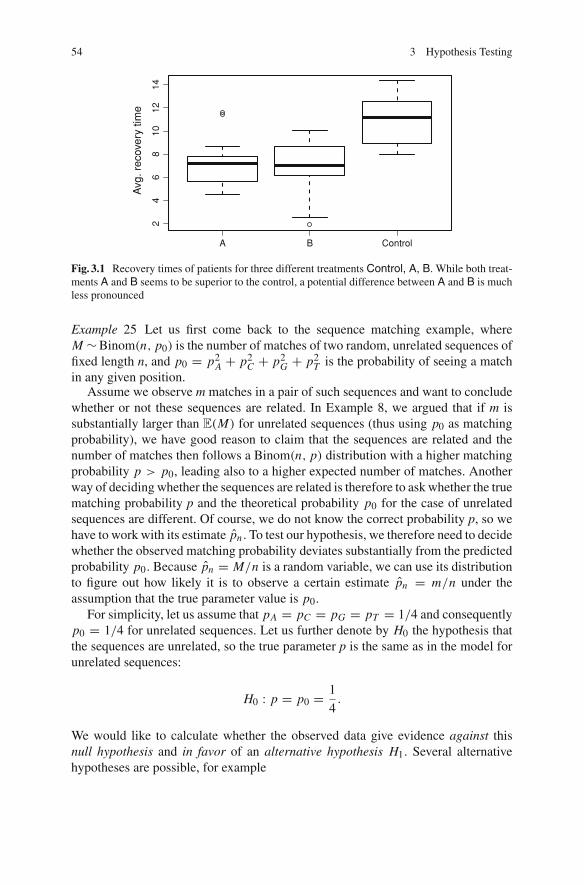
54 3 Hypothesis Testing

A B Control

24

68

1012

14

Avg

. rec

over

y tim

e

Fig. 3.1 Recovery times of patients for three different treatments Control, A, B. While both treat-ments A and B seems to be superior to the control, a potential difference between A and B is muchless pronounced

Example 25 Let us first come back to the sequence matching example, whereM ∼ Binom(n, p0) is the number of matches of two random, unrelated sequences offixed length n, and p0 = p2

A + p2C + p2

G + p2T is the probability of seeing a match

in any given position.Assume we observe m matches in a pair of such sequences and want to conclude

whether or not these sequences are related. In Example 8, we argued that if m issubstantially larger than E(M) for unrelated sequences (thus using p0 as matchingprobability), we have good reason to claim that the sequences are related and thenumber of matches then follows a Binom(n, p) distribution with a higher matchingprobability p > p0, leading also to a higher expected number of matches. Anotherway of deciding whether the sequences are related is therefore to ask whether the truematching probability p and the theoretical probability p0 for the case of unrelatedsequences are different. Of course, we do not know the correct probability p, so wehave to work with its estimate pn. To test our hypothesis, we therefore need to decidewhether the observed matching probability deviates substantially from the predictedprobability p0. Because pn = M/n is a random variable, we can use its distributionto figure out how likely it is to observe a certain estimate pn = m/n under theassumption that the true parameter value is p0.

For simplicity, let us assume that pA = pC = pG = pT = 1/4 and consequentlyp0 = 1/4 for unrelated sequences. Let us further denote by H0 the hypothesis thatthe sequences are unrelated, so the true parameter p is the same as in the model forunrelated sequences:

H0 : p = p0 = 1

4.

We would like to calculate whether the observed data give evidence against thisnull hypothesis and in favor of an alternative hypothesis H1. Several alternativehypotheses are possible, for example

3.1 Introduction 55

• the simple alternative H1 : p = 0.35,• the composite and one-sided alternative H1 : p > 1

4 ,• the composite and two-sided alternative H1 : p �= 1

4 .

Each of these alternatives claims that the probability for a match in the two sequencesis a certain parameter p, and gives valid ranges for this parameter. While the simplealternative claims a specific value, the composite alternatives give whole ranges offeasible values. More general, we can also define two (disjoint) sets �0 and �1such that the null- and alternative hypotheses are H0 : p ∈ �0 and H1 : p ∈ �1,respectively.

Intuitively, consider sequences of length n = 1000 with m = 100 observedmatches. With pn = 1/10, this indicates that the matching probability is actuallymuch smaller than p0 = 1/4. However, with the alternative H1 : p > 1/4, this datawould not give evidence against H0. This does not mean that H0 is true (which clearlyisn’t the case here), but that the alternative H1 cannot explain the data any better thanH0. On the contrary, if we test H0 against the two-sided alternative H1 : p �= 1/4,there is sufficient evidence that this alternative provides a better explanation for thedata, so we would reject the null hypothesis.

To make these considerations more quantitative and rigorous, let us use the one-sided alternative H1 : p > 1/4, so we only need to check if we observe unusuallymany (and not perhaps unusually few) matches. Consider the following argument:if H1 is true, we expect to see more matches than if H0 were true. However, thenumber of matches is random, and there is the possibility that even if H0 is true,the observed counts are high just by chance. Knowing the distribution of M underH0 (i.e., with p = p0 = 1/4), we can compute the probability that M exceeds anobserved number m of matches under H0; this is the probability that the distributionstated in H0 gives rise to data at least as extreme as observed. If this probability isvery low, this indicates that the null hypothesis is unlikely to be true, as it is unlikelythat the data have been generated with the stated parameters.

We know that the number of matches has a Binomial distribution. If the nullhypothesis is true, we also know that the matching parameter p is equal to p0 = 1/4.

With this information, we compute the probability to see at least the observed numberof m matches, provided the null hypothesis is indeed correct, to be

P(M ≥ m|H0) = 1 − P(M < m|H0) = 1 −m−1∑i=0

(n

i

)pi

0(1 − p0)n−i ,

where we slightly abuse the notation for conditional probabilities for brevity.For Example 8, we considered sequences of length n = 100 and m = 29 observed

matches. The probability to see at least this number of matches in unrelated sequencesis P(M ≥ 29|H0) = 0.1495, which gives no evidence against H0 in favor of H1.

On the contrary, the probability to observe at least m = 50 matches in unrelatedsequences is P(M ≥ 50|H0) = 2.13e − 08, providing substantial evidence that H0is actually false.


The calculated probabilities P(M ≥ m|H0) are called p-values. To reject or notreject a given null hypothesis, we fix a probability α and compute a threshold c suchthat P(M ≥ c|H0) = α. We then reject H0 in favor of H1, if m > c and do notreject if m ≤ c, leading to the rejection region Rα = (c,∞). The probability α

describes the false positive errors, as it is the probability that we reject H0, althoughit is actually correct. For the example with sequence length n = 100 and a probabilityof α = 0.05, we calculate

P(M ≥ c|H0) ={

0.0693, for c = 32,

0.0446, for c = 33.

We would therefore use the more conservative c = 33 as our threshold, reject H0 :p = 1/4 in favor of H1 : p > 1/4 in the case m = 50 > c, and not reject in the casem = 29 < c.

Importantly, not rejecting is not the same as accepting H0 because if we do nothave evidence against H0, we cannot conclude that it is actually true. We shouldtherefore never speak of “accepting” the null hypothesis, but only of “not rejecting”.

3.2 The General Procedure

The considerations taken in the introductory example can be divided in the followingsteps, providing the general setup for testing statistical hypotheses.

1. Clarify assumptions on independence, sample sizes etc. This will guide the choicesin the next steps and is usually only done implicitly.

2. Formulate the null hypothesis H0 and the alternative hypothesis H1.

Choose H0 such that we retain it unless there is strong evidence against it. ChooseH1 to be simple or composite and one- or two-sided depending on the problem.

3. Choose a test statistic T = g(X1, . . . , Xn) as a function of the data Xi .4. Derive the null-distribution of T, i.e., its distribution P(T ≤ t |H0) under the

assumption that H0 holds.This is usually the difficult part. Of course, the choice of T above is alreadypartially guided by the necessity to determine its null-distribution. For manypractical purposes, steps 3 and 4 are done simply by looking up the appropriatetest.

5. Compute the test statistic’s value t = g(x1, . . . , xn) from the data x1, . . . , xn .6. Compute the p-value P(T ≥ t |H0).

The smaller the p-value, the less likely it is that the observed value t was generatedfrom the null-distribution.

Ultimately, the p-value gives us the information to either reject or don’t reject thenull hypothesis in favor of the alternative hypothesis. To arrive at such a decision froma given p-value, we decide on a level α for the test. This level gives the probabilityof getting a false positive, i.e., of falsely rejecting H0 although it is true, due to

3.2 The General Procedure 57

uncommonly large deviations of the observed test statistic t from the expected valueunder H0. Using this level, we then compute the rejection region Rα of T such thatwe reject the null hypothesis if the observed value t is inside the rejection regionRα , and do not reject if it is outside. This rejection region is computed from thedistribution of T under H0 and the two hypotheses. If the null hypothesis is rejectedat a level α, we say that the test is significant at level α.

The p-value corresponds to the smallest level α such that the test would not yetreject. For example, if we observe a p-value of 0.034, the test would reject at theα = 0.05 level, but not at the α = 0.01 level. Indeed, no R-implementation of astatistical test requires a test level; they all report the p-value, so we can decide whatto do.

Absence of evidence is not evidence of absence. Rejecting the null hypothesishinges on the distribution of the test statistic assuming H0 is true. The p-value givesthe probability that we see a value at least as extreme as the observed one under thisdistribution. It is not the probability that H0 is true. A very low p-value indicatesthat the test statistic is unlikely to take the observed value under H0 and thereforeprovides good reason to reject it. On the contrary, a high p-value does not give proofthat H0 is actually true. In fact, it could be that the alternative just provides an evenworse explanation, or the test has very low power to distinguish the two alternatives.

As a consequence, a statistical test should always be stated such that the nullhypothesis defines the “status quo” and gets rejected if the desired result shows inthe data. Thus, testing for a difference between a default and non-default assumption,we would set H0 to state that there is no difference and reject this hypothesis in favorof the alternative that there is a difference. This way, we can quantify our level ofconfidence in the rejection by a low p-value. Would we set the no difference scenarioas alternative, we would aim at “proving” H0 with the data, which we can’t.

Very informally, let T be our test statistic with value t for some specific data. Then,we compute P(T ≥ t |H0), the probability to see this data if H0 is true, which is notP(H0|T ≥ t), the probability of H0 being true, given the data.

Stating the hypotheses. Stating a null hypothesis H0 to reflect the default assump-tions can become quite intricate for more involved problems. In particular, it mightnot be straightforward to formulate the hypothesis in terms of parameter regions oreven to find the formal statistical hypothesis that correctly reflects our verbal hypoth-esis on the data. This lead some researchers to introduce a type-III error (see Sect. 3.5for type-I/II errors), which is often stated as “asking the wrong question and usingthe wrong H0”, or “correctly rejecting H0, but for the wrong reasons”.

Additionally, we have also to take some care in stating a useful alternative hypoth-esis. As we already saw, the choice of the alternative partly determines the rejectionregion. For the case of one mean μ, the decision for a two- or a one-sided alternativecan usually be decided from the problem itself. However, imagine we were to test twomeans at the same time with null hypothesis H0 : μA > 0, μB > 0. A reasonablealternative is H1 : μA < 0, μB < 0, but it is very strict and we may want to relax itto H1 : (μA < 0 or μB < 0). Depending on which alternative we select, this leadsto different rejection regions.


3.3 Testing the Mean of Normally Distributed Data

One of the most frequent applications of statistical testing involves questions aboutthe location of a distribution. In particular, we are often interested whether the meanof a given sample deviates significantly from an assumed value or whether twosamples have the same mean. A typical example is the comparison of the result ofan experiment to a control. This control can either be an assumed model, predictingthe mean, or another experiment. In this section, we will discuss statistical tests toanswer these questions with decreasing amount of additional assumptions. We startwith a pedagogical example where we assume the distribution to be normal and thevariance to be known, before introducing the family of t-tests which allow us to useestimates for the variance.

These tests are not applicable for non-normal data and we should always checkthe data for normality before performing any of them. We can do this visually usinga normal quantile-quantile plot as introduced in Sect. 1.8.3. If the empirical quantilesdo not deviate too much from the straight line expected from a normal distribution,it is usually safe to use a t-test. Of course, “too much” deviation is pretty subjectiveand one should always provide the Q-Q-plot in addition to the test results. For a morequantitative check, we might use the Kolmogorov-Smirnov test for testing normalityin the data (Sect. 3.4.1) or the more specialized Shapiro-Wilks test (Sect. 3.4.2).

While not directly testing the mean, the Wilcoxon-test is often used for similarpurposes on non-normally distributed data; it will be introduced in Sect. 3.4.3. Wealso only consider the two-sample case with independent data. If the two sampleshappen to be paired, for example, by measuring the weight of the same set of peoplebefore and after a treatment and comparing the two values for each patient, a pairedt-test needs to be used.

3.3.1 Known Variance

Let us assume that we measure the weights x1, . . . , xn of n people from a particularregion. We claim that people are substantially heavier in this region than a particularweight μ0. Thus, our two hypotheses are informally “H0 : weights are pretty muchμ0” versus “H1 : weights are larger than μ0”. Note that the case of weights lowerthan μ0 is not covered.

Clarifying assumptions. We assume that we have reason to believe (or actuallychecked) that the measured weights follow a normal distribution, so Xi ∼ Norm(μ, σ 2). For simplicity, we further assume that we know the variance σ 2 and do notneed to estimate it from the data. Clearly, this is often an unrealistic assumption, andwe will discard it in Sect. 3.3.2.

Formulating the hypotheses. The two hypotheses can be formally written as

H0 : μ = μ0H1 : μ > μ0,

3.3 Testing the Mean of Normally Distributed Data 59

5 10 15 20 25 30

0.00

0.10

0.20

Value of test statistic

Den

sity

Fig. 3.2 Distribution of test statistic X under H0 : μ = μ0 = 10 (solid) and two values for thealternative: μ = 14 (dashed) and μ = 25 (dotted). Shaded areas correspond to a false positiveprobability of α = 0.05 (solid gray) and to a false negative probability of 0.118 for a true valueμ = 14 (dashed gray)

or equivalently

H0 : μ − μ0 = 0

H1 : μ − μ0 > 0.

The alternative is composite, as it encompasses a set of possible values, and one-sided, as it ignores the possibility that the data is actually smaller than the claimedvalue.

Choosing the test statistic. Since we do not know the true mean μ, we estimate itby x = μn , and thus compare a random number with the claimed mean μ0. This isan example where we use an estimator as the test statistic.

Deriving the distribution under H0. As an MLE, the arithmetic mean X itself hasa normal distribution with parameters E(X) = μ and Var(X) = σ 2/n (this is wherethe known variance comes into play: the normal distribution is only correct if we donot need to estimate the variance).

Fixing a test level α, and thus the allowed probability for a false positive, onlyrequires the distribution of X under H0, which in this case is X ∼ Norm(μ0, σ

2/n).The composite alternative describes a whole family of distributions, namely all nor-mal distributions with variance σ 2/n and any mean μ > μ0.

In Fig. 3.2, the distributions of X for n = 20 sample points and a variance ofσ 2 = 40 are shown for a true mean of μ = 10 (solid line), of μ = 14 (dashed line),and of μ = 25 (dotted line). Testing μ = μ0 = 10 thus leads to the null distributiondepicted by a solid line, while the dashed and dotted lines describe two distributionsout of infinitely many given in the alternative hypothesis.

Computing the rejection region. For an observed arithmetic mean x , the p-valuefor the test is P(μn ≥ x |H0) = 1 − �(x;μ0, σ

2/n). Let us fix a test level ofα = 0.05. The rejection region is easily calculated as (c,∞), where c is the valuesuch that P(X ≥ c|H0) = 0.05, which computes to

c = μ0 + z1−α

σ√n.


For the proposed α, we have z0.95 = 1.645, which for μ0 = 10 leads to the rejectionregion

R0.95 = (12.326,∞),

and we reject H0 : μ = μ0 = 10 if x > 12.326. For smaller differences, we do notreject.

The probability of a false positive for the level α = 0.05 is given in Fig. 3.2 by thesolid gray area. For a true value of μ = 14, this level leads to probability of 0.118for a false negative (H0 not rejected although false), given by the dashed gray area,and a false positive probability of 0 for a true value of μ = 25. We will come backto these two error probabilities in Sect. 3.5.

Equivalently, we can conclude that the normalized difference of observed andclaimed mean has a standard normal distribution,

T := X − μ0√1n σ

∼ Norm(0, 1), (3.1)

and we reject if its realization t exceeds the corresponding quantile, i.e., if

t > z1−α.

The two-sided alternative. If we test against the two-sided alternative H1 : μ �= μ0,the rejection region consists of two intervals, which contain values that are consideredtoo low and too high, respectively. Very similar to before, the rejection region Rα =(−∞, c1) ∪ (c2,+∞) is computed such that

P(X ∈ Rα|H0) = α

holds, which immediately leads to

Rα =(

−∞, μ0 + zα/2σ√n

)∪

(μ0 + z1−α/2

σ√n,+∞

).

We thus reject H0 if x ∈ Rα , or, equivalently, if |T | > z1−α/2, with T the normalizeddifference defined by (3.1). For the level α = 0.05 and parameters as before, the twocritical thresholds are c1 = 7.228 and c2 = 12.772.

Rejection regions and confidence intervals. There is a striking similarity betweenthe rejection region Rα of the test statistic T and the (1 − α)-confidence interval ofthe estimator X for the mean. Indeed, if we use any estimator θn directly as the teststatistic, we reject the null hypothesis H0 : θ = θ0 at the level α if θ is not containedin the (1 − α)-confidence interval of θn .


3.3.2 Unknown Variance: t-Tests

Clearly, the assumption that we do not know the mean of a sample—but exactly knowthe variance—is an oversimplification in most practical cases. We will therefore dropthis assumption and additionally estimate the variance from the data, which leads tothe t-distribution under the null hypothesis. The corresponding family of tests is thenknown as t-test. We describe these tests for three cases: (i) we test one sample meanfor a specific value, but need to estimate the variance, (ii) we test if the means oftwo samples are equal, with both samples having the same, but unknown variance,(iii) we test if the means of two samples are equal, each sample having unknownvariance.

We will again assume that the data X1, . . . , Xn (and Y1, . . . , Ym for the two-sample cases) are normally distributed with means μX and μY , and variancesσ 2

X and σ 2Y , respectively.

One sample with unknown variance. Let us consider n sample points from aNorm(μX , σ 2

X ) distribution, where both the mean μX and the variance σ 2X are

unknown and need to be estimated. We estimate σ 2X as before by

S2X = σ 2

X = 1

n − 1

n∑i=1

(Xi − X)2.

To test the hypothesis H0 : μX = μ0, we can again use the normalized difference

T = X − μ0√1n SX

between observed and expected mean as test statistic, this time replacing the vari-ance by its estimate. The test statistic T does not have a normal distribution, but at-distribution with n − 1 degrees of freedom. The reason for this is exactly the sameas for computing the confidence interval for the mean’s estimator X with estimatedvariance: the estimate of the mean from the data became more uncertain, leading toslightly heavier tails of the distribution. We consequently reject in favor of the two-sided alternative H1 : μX �= μ0 if the normalized difference of claimed and observedmean is too large and the absolute value of the test statistic therefore exceeds thecorresponding t-quantile:

Reject H0 ⇐⇒ |T | > t1−α/2(n − 1),

and similarly for the one-sided alternatives.

Example 26 With 10 random samples from a Norm(15, 40) distribution, the testH0 : μX = 10 against the two-sided alternative H1 : μX �= 10 gives a p-valueof 0.02262 for the t-test, but a too low p-value of 0.00302 when using the normaldistribution with estimated variance.


Two samples with unknown and unequal variances. In practice, one is often inter-ested in testing whether two samples differ significantly in their mean rather thantesting one sample mean against a given value. As an example, we might have somedata Xi from an experiment and some data Yi from a control, and ask whether thereis any difference in the samples’ means. This is known as a two-sample test problem.Formally, we like to test H0 : μX = μY against the alternative, e.g., H1 : μX �= μY .Moreover, the samples are allowed to be of different size. As before, our test sta-tistic will be the difference of the two estimated means. Because both estimatorsare maximum-likelihood and therefore have a normal distribution, their differenceis also normally distributed. The only thing we need to figure out is the variance ofthis difference, so we can normalize correctly to get a standard normal distributionfor the estimator. Recalling the elementary properties of the variance, the varianceof the difference is quickly established:

Var(X − Y ) = Var(X) + Var(−Y ) + 2Cov(X , Y ) = Var(X) + Var(Y ),

because the X and Y samples are independent and thus Cov(X , Y ) = 0. Thus,

Var(X − Y ) = S2X

n+ S2

Y

m

is an estimator for the variance of the difference, which immediately leads to the teststatistic

T = X − Y√1n S2

X + 1m S2

Y

.

However, computing the correct distribution of this test statistic is quite tedious andyields a formula that contains the true parameter values, which are of course notavailable. In practice, this distribution is therefore approximated by a t-distributionwith ν (or less) degrees of freedom, where ν is computed as

ν =

(S2

Xn + S2

Ym

)2

S4X

n2

n−1 +S4Y

n2

m−1

,

and we reject H0 : μX = μY if |T | > t1−α/2(ν) in favor of H1 : μX �= μY . Mostimplemented versions of this test, such as the functiont.test() inR, automaticallydecide on the correct test statistic and the relevant parameters.

Two samples with unknown but equal variances. If the two variances are expectedto be equal or at least very similar, we can replace the two individual estimatesS2

X and S2Y by the pooled variance

S2XY = (n − 1)S2

X + (m − 1)S2Y

n + m − 2.


This estimate looks quite similar to the usual estimate of a variance: we “lost” twodegrees of freedom, one for each arithmetic mean and consequently divide by thetotal degrees of freedom from the overall sample, m +n−2. The test statistic is againthe difference of the two observed means, normalized by the standard deviation ofthis difference:

T = X − Y√1n + 1

m SXY

.

This test statistic has a t-distribution with m + n − 2 degrees of freedom and wereject H0 : μX = μY if |T | > t1−α/2(m + n − 2) in favor of H1 : μX �= μY .

Example 27 As a very brief example, let us look at a t-test performed on two setsof samples with n = 10 samples from a Norm(10, 40) distribution and m = 13samples from a Norm(12, 30) distribution. In practice, we would not know the correctdistributions and want to test whether the two sample means differ significantly. Forthis, we perform a two-sided t-test with null hypothesis H0 : μX − μY = 0 versusthe alternative H1 : μX − μY �= 0. Using the R implementation of this test, we getthe following report:

Welch Two Sample t-test

data: x and yt = -2.0876, df = 15.988, p-value = 0.0532alternative hypothesis: true difference in means is notequal to 095 percent confidence interval:-9.96370876 0.07680932sample estimates:mean of x mean of y7.705368 12.648818

In the first line, R informs us that it uses a variant of the t-test, known as theWelch-test, here in its two-sample form. It then reports the data used, the values forthe test statistic, the estimated degrees of freedom, and the p-value. We note thatthe degrees of freedom are not integer, but were calculated using an interpolationformula due to the different sample sizes and variances. After giving the alternativeused, it reports the 95% confidence interval for the test statistic and finally the twoestimated means. Note that the confidence interval is for the difference in means andshould contain 0, if the means are the same. The test gives a p-value of 0.0532, whichis significant at the α = 0.1, but not the α = 0.05 level.


3.4 Other Tests

Apart from testing the mean of one or two samples, there are many more hypothesesthat can be tested using suitable test statistics. In this section, we will introduce asmall variety of such tests and briefly explain their major ideas.

3.4.1 Testing Equality of Distributions: Kolmogorov-Smirnov

The Kolmogorov-Smirnov (KS) test checks whether a sample follows a given distri-bution (one-sample version) or if two samples are equally distributed (two-sampleversion). The test statistic is the maximal difference (technically: the supremumof the difference) of the empirical cumulative distribution function and the givendistribution function:

D := supx

∣∣∣Fn(x) − F(x)

∣∣∣ .

This difference takes values between zero and one and is larger, the more the sampledistribution deviates from the given one.

The KS-test works for any distribution. However, the distribution function F hasto be completely specified by explicitly stating all parameter values.

The two-sample version tests the two empirical cdfs F and G:

D := supx

∣∣∣Fn(x) − Gn(x)

∣∣∣ .

An example is given in Fig. 3.3, where 20 exponentially distributed sample pointsare generated for λ = 3 and their ecdf compared to the cdf of a normal distributionwith parameters μ = 0.5 and σ 2 = 0.1. The largest difference is D = 0.3983 foundat x = 0.4213, leading to a p-value of p = 0.002248. This indicates strong evidenceagainst the null hypothesis and we would conclude that the distributions are indeeddifferent.

3.4.2 Testing for Normality: Shapiro-Wilks

Normality of the data is a very common assumption for statistical tests andprocedures. The Shapiro-Wilks test provides a more specialized alternative to theKolmogorov-Smirnov test for testing if the data is indeed normally distributed. Thistest compares the variance of the data, estimated as s2 = 1/(n − 1)

∑i (xi − x)2,

with the variance expected by a normal distribution. For computing this expectedvariance b2, the test uses the same method as a normal Q-Q-plot and estimates the

3.4 Other Tests 65

0.0 0.5 1.0 1.5 2.0

0.0

0.4

0.8

Value

(E)C

DF

s

●

●

●

●

●

●

●

●

●

●

●

●

●

●

●

●

●

●

●

●

Fig. 3.3 Kolmogorov-Smirnov test. The empirical cdf of 20 Exp(3) samples (black dots and lines)is compared to the theoretical Norm(0.5, 0.1) cdf (dashed line). The test statistic measures thelargest absolute difference D = 0.3983, found here at 0.4213 and denoted by a dotted vertical line

slope of the normal Q-Q-line (see Sect. 1.8.3). The test statistic is then the quotientof the two variances

W = b2

(n − 1)s2 ,

and we test H0 : W = 1, expected if the data is normal, against H1 : W �= 1. This testgenerally performs better than the corresponding KS-test and should be preferred,especially for small sample sizes. A sample size of n ≥ 3 is necessary for the test towork, and an upper limit is given with n ≈ 3000.

3.4.3 Testing Location: Wilcoxon

For testing whether two distributions are equal, we can also rely on anothernon-parametric test known as the Wilcoxon or Mann-Whitney-U test. While not test-ing the location itself but rather the whole distributions, this test can neverthelessoften be used as a non-parametric alternative to the t-test family if the data is notnormally distributed, provided the variances in the samples are of comparable sizeand the sample distributions are similar enough such that the differences are mainlycaused by different locations.

The main idea of the Wilcoxon test is the following: let us again assume thatX1, . . . , Xn and Y1, . . . , Ym are two samples of size n and m, respectively, and let usagain denote by X(i) the ith smallest sample point, which we say to have rank i. Wenow join the samples into a new sample Z and denote by Z(i) the ith smallest samplepoint in the joint sample, so i runs from 1 to n + m. Provided the two samples havesimilar distributions, the ranks of the two individual samples within the joint sampleshould distribute equally and we expect to see a good “mixing” of the two samplesin Z.


The Wilcoxon test now compares the sum of the ranks of X and Y in Z to decidewhether this is indeed the case. For this, let us denote by RX the sum of all ranksof elements of the X sample in the ordered joint sample Z. In practice, we checkwhether Z(i) originally belonged to the X and if so, we add i to the sum, until wereach the (m + n)th element of Z. Similary, let us denote by RY the sum of ranks ofthe Y samples in Z, established by the same procedure.

The sum of all ranks is then

RX + RY =n+m∑i=1

i = (n + m)(n + m + 1)

2,

and the first sample of size n provides the fraction nn+m of the joint sample. Further,

RX is bounded by

n∑i=1

i = n(n + 1)

2≤ RX ≤ nm + n(n + 1)

2,

as one easily verifies: the lower bound gives the case that the Xi form the first nelements of the joint sample, i.e., are all lower than the Y j , whereas the upper boundgives the case that the Xi are all greater than the Y j .

We then form the respective difference of the actual rank-sum from the upperbound:

UX = nm + n(n + 1)

2− RX and UY = nm + m(m + 1)

2− RY ,

and use the minimum of these two differences as our test statistic

U := min(UX , UY ).

For small n and m, the null-distribution P(U = u|H0) can be tabulated by exhaus-tively computing all cases and counting. For large n and m, the null-distribution isvery close to a normal distribution and it suffices to compute its mean and variance.Provided the null hypothesis H0 of equal location is true, we expect the ordered Xsample to be uniformly dispersed in the ordered Z sample and thus

E(RX ) = n

n + m(RX + RY ) = n(n + m + 1)

2,

in which case the variance of the rank-sum is

Var(RX ) = nm(n + m + 1)

12,

and similarly for RY . The desired expectation and variance for U are then easilycomputed.

3.4 Other Tests 67

t-or Wilcoxon test? The t-test is slightly more sensitive to false positives thanthe Wilcoxon-test for normally distributed data, but this advantage decreases rapidlyas the data deviates from normality. The Wilcoxon-test performs much better onnon-normal data and is available in as many variants (one- and two-sided, multidi-mensional, paired observations, etc.). The Wilcoxon-test is also more conservative: ifwe reject using this test, we would also always reject using a t-test. We can thereforealmost always use the Wilcoxon-test, unless we are very sure that the data is normallydistributed, the variances of the two samples are very different, or we explicitly wantto test the mean(s).

3.4.4 Testing Multinomial Probabilities: Pearson’s χ2

For multinomial data, like the nucleotide counts in a sequence of length n, we mightwant to test whether the probabilities for each category follow a particular distrib-ution, given by the probabilities (p0

1, . . . , p0s ). For example, one might want to test

the hypothesis that the nucleotide frequencies in the sequence are all equal by testingthe null hypothesis

H0 : (pA, pC , pG , pT ) = (p0A, p0

C , p0G, p0

T ) = (1/4, 1/4, 1/4, 1/4)

against the alternative

H1 : (pA, pC , pG , pT ) �= (1/4, 1/4, 1/4, 1/4).

In contrast to previous examples, we test all probabilities simultaneously. Pearson’sχ2-test compares the expected number of counts in each category to the observedcount xi . The expected count under the null hypothesis is E(Xi ) = np0

i . The χ2-teststatistic is then given by the sum of normalized differences

T =s∑

i=1

(Xi − np0

i

)2

np0i

and has a χ2(s − 1) distribution under the null hypothesis.

Example 28 Recall that Gregor Mendel studied peas in order to find the laws ofinheritance. More specifically, he cross-bred peas and observed counts for two fea-tures, namely round/wrinkled and yellow/green, leading to four categories whichwe abbreviate as ry,rg,wy,wg, respectively. The theory of inheritance leads to theprediction that the frequencies for these categories should be

(p0r y, p0

wy, p0rg, p0

wg) = (9/16, 3/16, 3/16, 1/16) .

In his original publication [1], Mendel studied n = 556 peas and observed the countsx = (315, 101, 108, 32). This leads to a value of t = 0.47 for the test statistic. Using


the χ2-distribution with 3 degrees of freedom, the critical value for a test level ofα = 0.05 is given by the 0.95-quantile χ2(3, 0.95) = 7.815, and we do not reject thenull hypothesis. Indeed, the p-value for this data is 0.95. As we discussed in Sect. 3.2,however, this does not necessarily mean that we have evidence in favor of H0.

3.4.5 Testing Goodness-of-Fit

The χ2-test can also be used as a goodness-of-fit test. This type of test is used forexample to check whether some data is in agreement with given predicted valuesfrom a model. In the above example of Mendel’s peas, the model of inheritancesuggests a certain number of observations in each category, and the test comparesthis predicted numbers with the observed ones.

Let us assume that a model predicts that the results follow a certain distributionwith density function f (x; θ). The l parameter(s) θ are not known. As an example,we might predict that the data is normally distributed, in which case θ = (μ, σ 2) arethe l = 2 unknown parameters.

For sample data x1, . . . , xn , the probability to see each particular sample point xi

is zero for a continuous distribution. The main idea is thus to discretize the result bysplitting the range of possible values into s non-overlapping intervals and count thenumber of observations in each interval. With I j the jth such interval and some fixedparameters θ ,

p j (θ) =∫

I j

f (x; θ)dx

is the predicted probability to see an observation in this interval and we wouldtherefore expect to see np j (θ) observations using this parameter value.

We can now compare this expected number of observations with the observednumber using the test statistics

T =s∑

i=1

(N j − np j (θ)

)2

np j (θ),

which has a χ2-distribution with s − 1 − l degrees of freedom.We are left with finding a general way to estimate the parameters θ . For reasons

that cannot be properly explained here, the MLE is not a good choice, as it does notnecessarily lead to a known (let alone χ2) distribution of T under the null hypothesis.Instead, we estimate the parameters such that they maximize the objective function

Q(θ) =s∏

j=1

p j (θ)N j ,

which then leads to the desired χ2-distribution of the test statistics.

3.4 Other Tests 69

Again, absence of evidence is not evidence of absence, and if the data does notgive evidence to reject H0, we cannot conclude that the hypothesis is actually correct.This is a major drawback of goodness-of-fit testing: We can only use it to check ifthe model could potentially explain the data, but we cannot rule out that there areother models that might fit as good. As the alternative is two-sided and composite,we also cannot flip the hypothesis, as we would need to know the distribution of Tunder this two-sided composite hypothesis.

3.5 Sensitivity and Specificity

In any hypothesis testing procedure, there are two types of errors that occur due to thefact that the test statistic is a random variable. There is the possibility that althoughH0 is true, we observe many unusual values in the data just by chance, leading toan incorrect rejection of H0. This is called a false positive or a type-I error. On theother hand, there is also the possibility that H0 is false, but again the sample valuessuggest that it is correct, so we would incorrectly not reject H0, which is called afalse negative or type-II error. Correctly rejecting or not rejecting H0 is called a truepositive and true negative, respectively. An example for type-I and type-II errors isalready given in Fig. 3.2, where we tested the mean of a normal random sample withknown variance. The four possible outcomes of a hypothesis test are given in thefollowing table:

H0 true H0 falsedont’t reject H0 true negative (TN), false negative (FN),

specificity 1 − α type-II error (β)reject H0 false positive (FP), true positive (TP),

type-I error (α) sensitivity 1 − β

The probability 1 − β to not make a type-II error is often referred to as the powerof the test; it is a function of the true value θ of the tested parameter. Formally,the power function η(θ) is the probability that the test statistic takes a value in therejection region, provided that H1 is true:

η(θ) := 1 − β(θ) = P(θn ∈ Rα|H1).

The power of a test is also called its sensitivity, as it gives the probability to correctlyreject the null hypothesis if the alternative is true and therefore describes how sensitivethe test is to the alternative. In addition, the probability 1 − α of not making a type-Ierror, and therefore correctly not rejecting H0 when it is true, is called the specificityof the test, as it describes how good the test can identify H0 among the alternatives.Choosing a test level α therefore prescribes a fixed specificity for the test.

Specificity and sensitivity are adversaries: making one of them very high usuallyreduces the other. Take the following test as an example: the null hypothesis is alwaysaccepted, no matter how the data look like. Clearly, this test is very specific: it alwayscorrectly detects the null hypothesis if it is true. On the other hand, it never correctly


6 8 10 12 14

0.0

0.4

0.8

True value of test statistic

Pow

er fu

nctio

n

6 8 10 12 14

0.0

0.4

0.8

True value of test statistic

Pow

er fu

nctio

n

Fig. 3.4 Power functions η(μ) for true mean μ0 = 10 and variance σ 2 = 40. Left: One-sided H1 :μ > μ0 (solid line) and two-sided H1 : μ �= μ0 alternatives (dashed line) for n = 20 and α = 0.05.Right: two-sided alternative for n = 20 and α = 0.05 (dashed black line), n = 100 and α = 0.05(dashed line), and n = 20 and α = 0.001 (dotted line)

detects the alternative and thus has very low sensitivity. Indeed the specificity is one,the maximal possible value, while the sensitivity is zero, the minimal possible value.Always rejecting the null hypothesis gives the inverse picture.

Example 29 In Sect. 3.3.1, we tested whether the mean of a normal sample was equalto a given value. The power of this test is η(μ) = 0.882 for μ = 15 and η(μ) = 1for μ = 25 (Fig. 3.2). The power function is

η(μ) := 1 − β(μ) = P(X > c|H1),

where μ is the correct parameter value under H1. The power is lowest if the trueparameter of the alternative is close to the assumed value of the null hypothesis andit is difficult to distinguish data produced under either hypothesis. The larger thedifference, the higher the power. For a difference of true and estimated parametervalues μ − μ0 > 5, the two-sided test reliably detects the alternative. The one-sidedtest has very low power for true values smaller than μ0, as it does not test against thesevalues. Almost none of these values would lead to a test statistic inside the rejectionregion, so the test will not reject H0. This is correct: the one-sided alternative doesnot provide a better explanation of the data than the null hypothesis in this case.

We compute the power function of the one-sided test as η(μ) = 1 −�(c;μ, σ 2),where again c = μ + z1−ασ/

√n is the critical value at the given test level.

The power function for the two-sided alternative is η(μ) = 1 − (�(ch;μ, σ 2) −�(cl;μ, σ 2)), where cl = μ + zα/2σ/

√n and ch = μ + z1−α/2σ/

√n are the

low and high critical value, respectively. The resulting functions are given in Fig. 3.4(left) for the one-sided alternative H1 : μ > μ0 (solid line) and for the two-sidedalternative H1 : μ �= μ0 (dashed line).

For a larger sample size of n = 100, the power of the test improves, as shown bythe dashed line in Fig. 3.4 (right). The power function gets narrower, meaning thatthe test has better sensitivity closer to the value of H0, and can thus better distinguishH0 and H1 in this range. Decreasing the test level to α = 0.001 (at sample size

3.5 Sensitivity and Specificity 71

n = 20) makes the alternative more difficult to distinguish for values near μ0, butmuch better further away (dotted line). Note that for μ = μ0, the power functionalways takes value η(μ0) = α.

3.6 Multiple Testing

So far, we always assumed that we are given one or two samples and perform onetest on these samples. Many measurement techniques, however, generate massiveamounts of data on which thousands of tests are performed simultaneously. In biol-ogy, the microarray allows to measure thousands of genes from the same biologicalsample, and differences in gene expression are tested for each individual gene. Thegenome of the fruit-fly, for example, has around 14,000 genes, which are all measuredon one array. Assuming we test for differences in gene expression using Wilcoxontests at a level of α = 0.05, we would already expect to see 14,000 × 0.05 = 700false positives, i.e., tests which claim that there is a significant difference betweencontrol and experiment, when in fact the difference is just by chance more extremethan expected. Because each of these 700 test results would lead to time-consumingand expensive follow-up experiments, we need to think about techniques that wouldallow us to deal with multiple tests in a useful way.

General Setting. Let us assume that we perform k tests simultaneously. Let V bethe number of false positives, U the number of true positives, and S, T the numberof true and false negatives, respectively, with k0 correct and k − k0 incorrect null-hypotheses. Importantly, we do not know k0, but can of course observe the constantk and the realization r of R, the number of rejected hypotheses.

H0 true H0 false

don’t reject H0 U (TN) T (FN) k − Rreject H0 V (FP) S (TP) R

k0 k − k0 k

There are two general strategies to cope with the problems posed by multipletesting: the family-wise error rate (FWER) tries to correct the individual test levelsα such that an overall test level of α∗ is achieved. Basically, these approaches try tocalculate new test levels such that the chance of even one false positive is smallerthan α∗ and thus

FWE = P(V > 0) ≤ 1 − (1 − α)k = α∗.

One such approach is the Bonferroni-correction, discussed below in Sect. 3.6.1. Thisapproach works well if the number of tests is comparatively small.

More recently, Benjamini and Hochberg introduced the concept of a false-discovery-rate (FDR), which works remarkably well even for a large number oftests. We will discuss the details in Sect. 3.6.2. In essence, the FDR is the expectedfalse discovery ratio of false and all positives:


FDR = E

(V

R

)= E

(V

S + V

).

This method explicitly allows a certain number of false positives to occur and aimsat controlling the fraction of false over all positives by recalibrating the individualp-values.

3.6.1 Bonferroni-Correction

Provided we are only interested in performing a small number of tests on the data,we can use the conservative Bonferroni-correction. This correction implements astrategy to control the family-wise error rate. Here is the idea: let Fi be the eventthat hypothesis i is a false positive (it is rejected although it is actually true). Theprobability to have at least one such false positive in k tests is then

P(V > 0) = P

(k⋃

i=1

Fi

)≤

k∑i=1

P(Fi ) =k∑

i=1

α = kα = α∗.

To guarantee an overall prescribed test level of α∗, we therefore perform each indi-vidual test at level α∗/k and reject the ith null hypothesis if its p-value pi is smaller,i.e., if

pi <α∗

k.

The Bonferroni-correction is very conservative as it tries to bring the overallprobability of even one false positive down to α∗. Additionally, the inequality com-pares the true probability of the Fi to the case that the Fi are all independent, anddoes not try to capture the dependencies. This yields the new individual test levelof α∗/k, which in many cases is much lower than would be required. For the intro-ductory microarray example, we have k = 14,000 individual tests. For an overallfalse positive probability of α∗ = 0.05, we thus need an individual test level ofα∗/k = 0.05/14,000 ≈ 4e − 06, which is unrealistic to yield any meaningfulresults.

3.6.2 False-Discovery-Rate (FDR)

Instead of correcting the test levels such that the overall false positive probabilityis kept below a given threshold α∗, we can try to explicitly allow false positives tooccur, but to control their expected fraction among all positives. This false discoveryrate (FDR) is given by FDR = E (V/R). Again, the number of tests k is known,

3.6 Multiple Testing 73

and the number of rejected hypotheses R is a random variable whose realization rcan be observed. On the other hand, the number of false positives V is also a randomvariable, but its realization can not be observed. Intuitively, if we would pick oneof the rejected hypotheses at random, the FDR can be interpreted as the expectedchance that this hypothesis was falsely rejected. For 100 rejected hypotheses, anFDR of 0.05 would also mean that we expect that 100 × 0.05 = 5 of these are falsepositives. To achieve a certain FDR in a concrete situation, we need to choose thenumber of rejections such that the prescribed FDR is reached; we can do this byappropriately adjusting the p-value for which to reject.

Benjamini-Hochberg procedure. We would like to have strategy that guarantees aproportion of false positives of at most q∗ among all rejected hypotheses. For this, wecalculate at which p-value to reject a hypothesis such that the FDR stays below thisdesired threshold q∗ as follows: we expect E(V ) = αk false positives in k tests for agiven test level α. For a given set of data, the number of null hypotheses rejected atthis level is r(α), a realization of R. The Benjamini-Hochberg procedure computesthis number r(α) such that the maximal number of hypotheses are rejected whilestill keeping the expected proportion of false positives below the given threshold q∗,thus

E

(V

R

)= αk

r(α)≤ q∗.

Let again pi be the p-value of the ith hypothesis test and consider the ordered p-valuesp(1) ≤ · · · ≤ p(k). We then compute the largest index l such that

p(i) ≤ i

kq∗

for all (i) < l. The values qi = ik q∗ are sometimes called the q-values. One can

show that if we reject those null hypotheses for which pi ≤ ql = lk q∗,

FDR ≤ k0

kq∗ ≤ q∗,

which guarantees the desired proportion of false positives.Comparing p-values and q-values. Despite some similarities, p-values and

q-values have some fundamental differences. The p-value gives the smallest testlevel at which not to reject and thus needs to be correct and exact to assess the data.On the other hand, q∗ is a threshold for an expected ratio, so the actual ratio might behigher. It serves more as a “calling” tool that filters out uninteresting test results froma large number of performed tests. A proper analysis would then further investigatethe remaining candidates, so it is usually not problematic if the desired q∗ is notexactly achieved in the actual study.

Example 30 Let us consider the scenario that k = 10 individual tests were performedon data and that their ordered p-values p(i) are


0.00017, 0.003, 0.0071, 0.0107, 0.014, 0.32, 0.4, 0.54, 0.58, 0.98.

For an overall test level of α∗ = 0.05, the Bonferroni correction then requiresindividual test levels of α = α∗/k = 0.005 and we would reject the first 2 nullhypotheses. On the other hand, we could decide to allow an expected fraction ofq∗ = 0.05 false positives among all rejected hypotheses. Using the Benjamini-Hochberg method, we compute the corresponding q-values to be

0.005, 0.01, 0.015, 0.02, 0.025, 0.03, 0.035, 0.04, 0.045, 0.05,

and p(5) = 0.014 < 0.025 = q5 whereas p(6) = 0.32 > 0.03 = q6; we wouldconsequently be able to reject the first 5 null hypotheses.

3.7 Combining Results of Multiple Experiments

Let us imagine that three groups independently did a particular experiment and eachgroup performed the same test on their data. The reported p-values are 0.08, 0.06,and 0.07, respectively, none of them significant at the α = 0.05 level. However, wemight argue that it seems unlikely that all three tests are so close to the 0.05-leveljust by chance and that combined, the three tests actually give significant evidenceto reject the null hypothesis.

We can invoke the following argument to justify this idea: let ti be the value ofthe test statistic Ti of test i, leading to a p-value of pi , and let us again assume kindependent tests. If the null hypothesis were true in all cases, we can ask for thejoint probability of simultaneously observing the given values of the test statistics:

P(T1 > t1, . . . , Tk > tk |H0) =k∏

i=1

P(Ti > ti |H0),

which corresponds to asking for the probability that the observed p-values occurunder H0.

Let Pi be the p-value of the ith test, treated as a random variable. It can be shownthat the Pi are uniformly distributed on [0,1] under H0 and thus each p-value isequally likely if the null hypothesis is correct. However, the product of uniformrandom variables is itself not uniform, so we need to calculate the correspondingdistribution. A simple trick comes to the rescue: the logarithm of a uniform randomvariable U, scaled by (−2), has a χ2-distribution with two degrees of freedom:

−2 log(U ) ∼ χ2(2),

and we know from Sect. 1.4 that the sum of χ2-variables still has a χ2-distribution,with corresponding degrees of freedom:

3.7 Combining Results of Multiple Experiments 75

Q = −2k∑

i=1

log(Pi ) ∼ χ2(2k).

This allows us to combine p-values from different experiments, provided the same testwas used in each experiment. We compute the realization q of Q from the observedp-values and reject the null hypothesis if q > χ2

1−α(2k).

Example 31 For the p-values 0.08, 0.06, and 0.07, we compute the value

q = −2 × (log(0.08) + log(0.06) + log(0.07)) = 15.9968

for the test statistic Q. With k = 3, this statistic has a χ2(6)-distribution, and theoverall P-value is thus p = P(Q > q|H0) ≈ 0.0138. While each individual resultdoes not give evidence against the null hypothesis, the combination of the threeexperiments shows significant evidence that the null hypothesis is false.

3.8 Summary

To test a property of a distribution, we formulate two hypotheses—the null hypothesisH0 and the alternative hypothesis H1—,such that the null hypothesis represents the“status quo”. We then compute the value for a test statistic T from a random sample;the distribution of T under the null hypothesis allows us to compute the p-value—theprobability of a false rejection. The smaller the p-value, the less likely H0 is true andwe reject it if the p-value is below a prescribed test level α. However, we can notprove the correctness of a null hypothesis and the p-value is not the probability thatH0 is correct.

Before choosing a test statistic, it is often worthwhile to check whether robustalternatives are available, such as the Wilcoxon-test to replace a classic t-test.

The sensitivity and specificity of a test describe the probabilities to correctly rejector not reject the null hypothesis. They depend on the test statistic, the two hypotheses,but also on the sample size.

When preforming several tests simultaneously, we need to recalibrate the p-valuesto correct for multiple testing, which we can do either by the Bonferroni-method,which controls the probability to get even one false positive, or using the false dis-covery rate approach, which allows a prescribed fraction of false positives among allrejected hypotheses.

Reference

1. Mendel, G.: Versuche über Pflanzenhybriden. Verhandlungen des naturforschenden Vereines inBrünn IV, 3–47 (1866)

Chapter 4Regression

Abstract Regression analysis describes the influence of covariates on a responsevariable. Two regression models are discussed: linear regression on one or severalcovariates and analysis-of-variance. Methods for estimating the respective modelparameters and hypothesis tests for eliminating non-significant covariates arepresented.

Keywords Linear regression · Model reduction · ANOVA

All models are wrong but some are usefulGeorge E. P. Box

4.1 Introduction

Regression analysis aims at studying the influence of one or more covariates X on aresponse Y. We only discuss parametric regression, where we know the functionalrelation between covariates and response, and try to identify the correct parameter(s)of this function. The regression function is then defined as the expected value condi-tioned on the values of the covariates:

r(x; θ) = E (Y |X = x) =∫

y f (y|x; θ)dy,

where f (y|x; θ) is the conditional probability density of Y |X with parameters θ.

Once we know the parameters, we can predict the average value for the responsefor any given values of the covariates by the regression function. For estimating theparameters from given data, we assume that we have n samples

(y1, x1,1, x1,2, . . . , x1,m), . . . , (yn, xn,1, xn,2, . . . , xn,m),


78 4 Regression

where yi is the value of the response variable in the ith measurement and xi, j is thevalue of the jth covariate for that measurement. Regression analysis assumes thatthe values of the covariates xi, j are known exactly. In contrast, the observed valuesof the response yi are subject to error and an error model is used to described theirdistribution around the true value. The assumed relation of covariates and responseis then

Y = r(x; θ) + ε,

where ε is a random error term.

Example 32 Let us consider the problem of finding the relation between the dryweight and height of a plant. We may claim that the dry weight increases linearlywith the height of the plant. Using the height as a covariate x and the dry weightas the response y, we can use the following linear regression model to describe thisrelation:

Y = β0 + β1x + ε.

Here, the parameter β0 is the dry weight of a plant with height zero, and β1 describeshow much more dry weight we get per increase in height. We implicitly assume thatthe height can be measured without error, but the measured weight spreads aroundthe true value by an error ε. The first task is then to measure the weight and height ofn plants, yielding the data (y1, x1) to (yn, xn). From this data, we would then try tofind the correct parameter values for β0 and β1. Once these are established, we canpredict the dry weight from the height of any new plant.

4.2 Classes of Regression Problems

Depending on the type of covariates and response, we can distinguish several classesof regression problems. The two main types are metric variables, which are any kindof (continuous) numbers, and categorial variables, which describe membership indistinct classes. Examples for the first type are measurements of length, (discrete)counts, and waiting times, for the second type categories such as male/female. Cate-gories can sometimes additionally have an order such as high > middle > low, andvariables are then called ordinal.

If both response and covariates are metric, we are in the setting usually calledregression, and we can further distinguish linear from nonlinear regression, dependingon the claimed functional relation r(). Linear regression is the typical first example ofregression methods and will be covered in detail in Sect. 4.3 for a single covariate. Ifseveral covariates are involved, powerful methods can be applied to reduce the modeland identify those covariates which have a significant influence on the response. Therequired methods for estimation and hypothesis testing are covered in Sect. 4.4.

4.2 Classes of Regression Problems 79

Regression of a metric response on categorial covariates requires Analysis-of-Variance (ANOVA). The impact of treatment (no drug / drug A / drug B) on therecovery time of a patient is an example. ANOVA can be seen as an extension oft-tests to more than two means; we discuss ANOVA in Sect. 4.5. After presentingthe estimators for the ANOVA model parameters, we also develop hypothesis teststo investigate the influence of combinations of groups on the response variable.

4.3 Linear Regression: One Covariate

We start by discussing linear regression with one covariate. This is the workhorse inregression analysis; it is widely applicable in practice and many other methods canbe derived as variants and extensions.

4.3.1 Problem Statement

Linear regression with one covariate assumes a regression function of the form

Y = β0 + β1 X + ε,

where Y is the metric response to the metric covariate X. The parameters (in linearregression traditionally called β) of this family of regression functions are theintercept β0 and the slope β1 of the (x, y)-line.

It is the error term ε that prevents us from observing the correct response directly,and makes Y a random variable. We assume the error to have zero mean, so it does notintroduce a bias in the analysis. We further assume that it has constant (but unknown)variance σ 2, independent of the value x of the covariate; this is called homoscedacity:

E(ε|X = x) = 0

Var(ε|X = x) = σ 2.

If the variance of the error does depend on the value x, we call this heteroscedacity.For some of the analyses, we do not need to assume a particular distribution of ε,

but for more sophisticated analyses, we often assume that the error has a normaldistribution. Section 4.3.3 is devoted to methods for checking these assumptions onthe error structure.

80 4 Regression

4.3.2 Parameter Estimation

Without assuming any particular error distribution, we cannot apply the maximum-likelihood principle and therefore rely on a least-squares method for estimating thetwo parameters β0 and β1. Given the parameter values, the value

yi = r(xi ) = β0 + β1xi

is the predicted response to the value xi of the covariate. We can apply least-squaresestimation to find those parameter values β0 and β1 that minimize the squared differ-ence ε2

i = (yi − yi )2 between the measured and the predicted value:

(β0, β1) = argminβ0,β1

n∑i=1

ε2i = argminβ0,β1

n∑i=1

(yi − (β0 + β1xi ))2 .

The differences ε2i are called the residuals and are themselves estimates of the error

ε in each sample point.This least-squares problem always has a unique solution and we even find explicit

formulas for the estimates:

β1 =∑n

i=1(xi − x)(yi − y)∑ni=1(xi − x)2

β0 = y − β1 x,

from which we can also estimate the variance of the error by

σ 2 = 1

n − 2

n∑i=1

ε2i ,

using n − 2 degrees of freedom (one less per estimated βi ).

Example 33 A typical example is shown in Fig. 4.1, where 10 responses weremeasured from a linear function y = β0 + β1x + ε with true parameters β0 = 2and β1 = 4 and normally distributed error with variance σ 2 = 40. Using the least-squares method, the parameters are estimated as β0 = −0.085 and β1 = 4.377. Theestimated standard deviation is σ 2 = 118.926. The solid line gives the predictedresponses yi for any value x of the covariate. The residuals εi are then the verticaldifferences between this line and the actual response value yi for a measurement,indicated by vertical dashed lines.

MLE under normality. If in addition to homoscedacity and unbiasedness, the erroris normally distributed, we can also apply the maximum-likelihood approach to findthe parameters β0, β1. Interestingly this yields the exact same estimators and thusmaximum-likelihood and least-squares estimates coincide under normality of errors.

4.3 Linear Regression: One Covariate 81

0 2 4 6 8 10−

1010

3050

x

y

Fig. 4.1 Linear regression of 10 measurements: Fitted regression y = β0 + β1x (solid line), resid-uals εi (dashed lines) and data (yi , xi ) (black points). True parameters are β0 = 2 and β1 = 4 withan error variance of σ 2 = 40 with estimates β0 = −0.085, β1 = 4.377, and σ 2 = 118.926

The MLEs for the two parameters are consistent and unbiased. As MLEs, theyalso have an asymptotic normal distribution, so confidence intervals for the estimatedparameters are given by

βi ± zα/2se(βi ),

where the estimators’ standard errors se(βi ) =√

Var(βi ) are

se(β0) = σ

σX√

n

√√√√1

n

n∑i=1

x2i ,

se(β1) = σ

σX√

n,

and σ 2X = 1

n−1

∑ni=1(xi − x)2 is the dispersion of values taken for the covariate.

We can even give the full covariance matrix, which contains the variance of the twoestimators in the diagonal, and the covariance of them in the off-diagonals:

Var

(β0

β1

)= σ 2

σX2n

(1n

∑ni=1 x2

i −x−x 1

).

Prediction intervals. Once the parameters are estimated from the data, we canapply this “fitted” regression model to predict the value Y∗ of the response for othervalues x∗ of the covariate by

Y∗ = β0 + β1x∗.

Although for given parameters this gives a particular prediction, this prediction stilldepends on the estimated values βi . Since these in turn depend on the original dataused for the estimation, the prediction Y∗ is still a random variable and we shouldcompute a confidence interval for Y∗ to quantify the confidence in the prediction.

82 4 Regression

This interval depends on the error ε, but also on the error in the estimates βi and isgiven by

Y∗ ± zα/2ζ ,

where the standard deviation ζ is not the estimated standard deviation of theestimator, but is given by

ζ 2 = σ 2( ∑n

i=1(xi − x∗)2

n∑n

i=1(xi − x)2+ 1

).

This confidence interval depends on the variance of the data, but additionally getswider, the further away the new covariate value x∗ is from the original values used inthe estimation of the parameters. For example, if values of the covariate in the originalsample are all between x1 = 1 and xn = 10, an extrapolation by predicting theoutcome for x∗ = 100 gives a much wider confidence interval than an interpolationat a value x∗ = 5.

4.3.3 Checking Assumptions

Application of standard linear regression techniques relies on two assumptions:homoscedacity of the data, i.e., constant variance independent of the covariate, and,for many conclusions, normally distributed errors. To check these assumptions, wecan perform an a posteriori analysis of the resulting residuals yi − yi after estimatingthe parameters.

Checking homoscedacity. Homoscedacity can be assessed by plotting the resid-uals εi of the fitted model against the covariate values xi . We then expect to seeno particular pattern and points should scatter uniformly around zero. If the vari-ance increases with the value of the covariate—one of the most common causesof heteroscedacity—a tilted ‘V’ pattern appears as the residuals get bigger withincreasing xi .

For 50 sample points using the same linear regression function as before, theresiduals are shown in Fig. 4.2 (left). Changing the error model such that the varianceincrease linearly with the covariate yields the tilted ‘V’ pattern in Fig. 4.2 (right).

Checking normality. Assessing whether the error distribution is normal is straight-forward once the model parameters are estimated. If the error distribution is normal,the resulting residuals should follow a normal distribution with mean μ = 0 and theestimated variance σ 2. We can use a normal Q–Q-plot for visual inspection. For theexample above with n = 50 sample points, the normal Q–Q-plots of the residualsare shown in Fig. 4.3 for both homoscedacity (left) and heteroscedacity (right). Inboth plots, the residuals scatter around a mean of zero, and do not introduce a biasin the estimation, as expected.

4.3 Linear Regression: One Covariate 83

−15

−10

−5

05

10

0 10 20 30 40 50Covariate i

Res

idua

l i

−60

0−

200

200

600

0 10 20 30 40 50Covariate i

Res

idua

l i

Fig. 4.2 Left Residuals εi of fitted model (points) spread around zero (dashed line) and show noparticular pattern. Right Residuals show heteroscedacity and form a titled ‘V’ pattern as the varianceincreases with increasing covariate

−2 −1 0 1 2

−15

−5

05

10

Normal Q−Q Plot

Theoretical Quantiles

Sam

ple

Qua

ntile

s

−2 −1 0 1 2−60

0−

200

200

600

Normal Q−Q Plot


Sam

ple

Qua

ntile

s

−10

Fig. 4.3 Normal Q–Q-plot of residuals in the case of homo- (left) and hetero-scedacity (right)

4.3.4 Linear Regression Using R

R already provides all necessary functions for easily fitting linear models. For givendata vectors x and y, a linear regression is fitted using the function lm(), whichrequires an R formula as input. R formulas are a very convenient way of representingcomplex regression problems. An example is

y ∼ x+ z,

which states that we want a fit of the response y on the two covariates x and z. Thus,R fits the model Y = β0 + β1 X + β2 Z by estimating the three parameters βi . InR formulas, the arithmetic operators +,−, ∗, / as well as exponents have specialinterpretations, and should not be confused with their usual meaning.

Parameter estimation. Let us consider a linear regression problem with onecovariate. The covariate vectorx contains the values of the covariate and the responsevector y the corresponding values of the response. Then, the R command

84 4 Regression

model <- lm(y ˜ x)

estimates the various parameters and yields a data-structure model containing allthe information about the resulting linear model.

Inspection plots. The model can then be plotted using the commandplot(model)to successively generate four plots: the residuals, the normal Q–Q-plot, the residualson another scale, and an influence plot (see Sect. 4.4.4 for a discussion of differentinfluence measures).

Model plot. We can also easily plot the model together with the data by firstplotting the data by plot(y ˜ x), and then adding the estimated regression linewith abline(model). This was done to generate Fig. 4.1.

Prediction. Predicting new values from a model is done using the predict()function, which expects a model data-structure and a data-frame with the new valuesof the covariates. For example

predict(object=model, newdata=new.x, interval=’prediction’)

for two new values x = 2.4 and x = 90 yields the result

fit lwr upr1 12.78273 −2.671691 28.237152 349.02757 217.846374 480.20877

with the predicted values in the first column and the lower and upper value of the0.95-prediction intervals in the second and third column.

4.3.5 On the “Linear” in Linear Regression

An important point to understand when using linear regression models is that weonly need the regression function to be linear in the parameters. For example, themodel

Y = β0 + β1 X2

is a perfectly valid linear regression model, because we may simply replace thecovariate X with a new covariate Z = X2 to get the familiar equation. Other modelscan be made linear by transformation. For example, the model

Y = β0 exp(β1 X)

is easily brought into a form suitable for linear regression by taking the logarithm.However, there is a caveat: if the original model has additive, normally distributederror, this error structure is also transformed by the logarithm and is no longer normal.This can cause major problems, as many of the statistics rely on normally distributedresiduals.

4.4 Linear Regression: Multiple Covariates 85

4.4 Linear Regression: Multiple Covariates

For more than one covariate, linear regression aims at fitting a hyperplane througha cloud of points. Again, all values of covariates are assumed to be fixed and non-random, and only the value of the response is subject to error.

Example 34 Let us reconsider our small introductory example of studying dry weightas a function of height in plants. Instead of using only the height, we may also want toconsider more variables that might have an influence on the dry weight. For example,we could study the influence of the amount of fertilizer on the weight. The modelwould then informally read

dry weight = β0 + β1 height + β2 fertilizer amount + error.

This allows us to ask more questions on the model, for example if the fertilizer hasany influence at all. If not, we could delete it from the model, which would result ina new and more simple model that is still able to sufficiently describe the dry weight.Regression analysis also allows us to explicitly take the influence of the covariateson each other into account. Here, we might consider that more fertilizer also yieldshigher plants, which we need to take into consideration when trying to find the mostsimple model that sufficiently explains the data.


We are studying a regression problem with m covariates X1, . . . , Xm and oneresponse variable Y. The data are again n tuples of sample points, each with onevalue for each covariate and one value for the noisy measured response. The regres-sion model is then of the form

Y = β0 + β1 X1 + β2 X2 + · · · + βm Xm + ε

and might additionally contain interaction terms to capture the dependency of covari-ates on each other. The resulting estimation problem of n equations in m covariatescan then be written as

⎛⎜⎝

y1...

yn

⎞⎟⎠ =

⎛⎜⎝

1 x1,1 · · · x1,m...

......

1 xn,1 · · · xn,m

⎞⎟⎠ ·

⎛⎜⎝

β0...

βm

⎞⎟⎠ +

⎛⎜⎝

ε1...

εn

⎞⎟⎠ ,

using matrix-vector notation. The matrix X containing the xi, j is called the designmatrix, where the first column is the “covariate” for the constant term β0. We againassume that each εi has mean zero and constant variance and that the errors are inde-pendent. For most of the statistics, we additionally require the errors to be normallydistributed.

86 4 Regression


We can again estimate the parameters as β = (β0, . . . , βm) by minimizing the sumof squared differences

β = argminβ

n∑i=1

(yi − (

β0 + β1xi,1 + · · · + βm xi,m))2

.

Again, the estimates can be given in explicit form by

β = (Xt X

)−1 XtY,

where X is the above design matrix containing the covariate values and a 1 entry inthe first column and Y is the vector containing the n values of the response.

4.4.3 Hypothesis Testing and Model Reduction

A natural question to ask is whether we really need all the covariates to explainthe measured responses, or if a smaller subset of covariates will already explain thedata. This is the question for a minimal adequate model, which is the model with thesmallest number of covariates that still explains the data reasonably well. In general,the data can always be better explained with more covariates, simply because weget more parameters to work with. However, reducing the model by eliminating onecovariate and its associated parameter might lead to a new model that is almost asgood as the larger model. For doing this properly, we need a way of quantifying whatwe mean by “almost as good”. We start with a central result on decomposing theoverall variation that will then naturally lead to the required statistics.

Decomposing the variation. Without considering any regression, the totalvariation in the response is

SStot =n∑

i=1

(yi − y)2.

It is proportional to Var(Y) with a factor of (n − 1) and is a measure of the overalldispersion of the response around its mean.

After fitting a regression model, this total variation can be decomposed into twocomponents: the explained variation or regression sum-of-squares

SSreg =n∑

i=1

(yi − y

)2,

which measures how much of the total variation can be explained by the fact thatthe measured response is actually spread around the regression line and not simplyaround its mean, and the error sum-of-squares


Fig. 4.4 (Adapted from [1])Total variation as sum ofexplained and unexplainedvariation. Each differenceyi − y of a measured to themean response can bedecomposed into thedifference yi − y of the meanand the predicted regressionvalue and the differenceyi − yi between predictedand measured value

4 5 6 7 8 9 10

1015

2025

3035

4045

Covariate x

Res

pons

e y

yi − y

yi − yiyi − y

yi

yi

y

SSerr =n∑

i=1

(yi − yi

)2,

which gives the unexplained variation still left, i.e., the dispersion of the measuredresponse values around their predicted values. Note that SSerr is exactly the residualsum-of-squares

∑i ε2

i that is minimized for estimation.Using the regression model, the total variation can always be written as the sum

of the explained and the unexplained variation:

SStot = SSreg + SSerr,

which is also demonstrated in Fig. 4.4.The variance can be recovered by dividing a variation by its corresponding degrees

of freedom, which are SStot : n − 1, SSreg : m, and SSerr : n − m − 1.

Varying the parameters βi of the regression function does not change the measuredresponse values, so the total variation SStot remains the same. However, we will alterthe predicted response values and thus the contributions of the explained and unex-plained variations to the total variation. A “good” set of parameters will have a largeSSreg, so a lot of the total variation is explained by the fact that the response spreadsaround the regression function rather than its mean. The remaining unexplainedvariation caused by this spread around the regression function is minimized in thiscase.

We can exploit this decomposition of the total variation in two ways: First, itgives the coefficient of determination R2 = SSreg/SStot, which is the proportionof explained to total variation. Consider using the model Y = β0 + ε with nocovariates, leading to the fit β0 = y with constant predicted response. The coefficientof determination is zero in this case and the model cannot explain any of the deviation

88 4 Regression

of measured yi from their mean. For a perfect linear fit with no measurement error,the coefficient is one, as the data is completely explained by the model. For a linearregression using a single covariate, the coefficient of determination is identical to thePearson’s correlation coefficient (see Sect. 1.6.4), given by

R2 = Cov(X, Y )

σXσY.

In addition to the coefficient of determination, we can also use the decompositionto compare models with a different number of covariates. For normally distributederrors, the various sum-of-squares all have χ2-distributions with appropriate degreesof freedom. Thus, the quotient

F = SSreg/m

SSerr/(n − m − 1)

of the explained versus the unexplained variation has an F(m, n−m−1)-distribution(see Sect. 1.4). The larger this value becomes, the better the regression explainsthe data.

Do we need any covariate? Now that we have worked out a way to quantify howgood a regression explains the data, we can start asking statistical questions on therelevance of the various covariates for this explanation. The boldest question is toask whether the regression actually explains the data at all. For this, we define thenull model Y = β0 + ε which in essence states that the data can be explained bythe spread around its mean alone. We then compare this null model to the full modelY = β0 + ∑

j β j X j + ε including all covariates. This comparison requires to testthe hypothesis

H0 : β1 = · · · = βm = 0

that it suffices to only consider β0 (i.e., the null model) estimated as β0 = y todescribe the data and the covariates thus have no relation to the response. With

F = SSreg/m


as our test statistic, we reject this null hypothesis if F exceeds the correspondingquantile of the F-distribution: F > F1−α(m, n − m − 1).

This hypothesis test can serve as a sanity check: if we do not find evidence toreject this hypothesis, the proposed model is not able to explain the data and none ofthe covariates has a significant (linear) relation to the response.

Testing subsets of covariates. The same ideas allow us to check if a reduced model,using only a subset of the covariates, already provides a sufficient fit to the data. Morespecifically, we want to test the hypothesis

H0 : βk+1 = · · · = βm = 0


that only the first k covariates are needed and the remaining m − k covariates donot provide any more explanation of the observed data. We only consider the firstcovariates simply to avoid clumsy notation; clearly, the exact same method worksfor any subset of covariates by simply re-ordering them.

Let us denote by SSreg(k) the explained variation of the reduced model, withonly the first k covariates present, and similar notation for the remaining variables.The special case SSreg(m) ≡ SSreg then denotes the previously explained variationof the full model.

The test statistic

Fk =(SSreg(m) − SSreg(k)

)/(m − k)


has a F(m − k, n − m − 1) distribution and we can reject the null hypothesis atthe level α if Fk > F1−α(m − k, n − m − 1). If we can reject H0, we concludethat the m − k covariates not contained in the reduced model do not significantlycontribute to the explanation of the data. Importantly, the term “significantly” iswell-defined in this context. By setting k = 0, we re-derive the previous hypothesisthat we do not need any covariate.

Model reduction. By exhaustively testing all possible reduced models, we cancompute a minimal adequate model; it has the smallest number of covariates suchthat adding any of the other covariates does not significantly increase the model’s fit.For m covariates, there are 2m different models from subsets of the covariates. Forlarger models, one therefore retreats to iterative procedures for finding a minimaladequate model. The two simplest procedures either start with the full model anditeratively discard one covariate at a time, or start with the empty model and iterativelyadd one covariate. The order in which this is done may however impact the result,especially if the covariates influence each other.

Example 35 Consider the following experiment: we want to investigate the influenceof the concentration x1, x2, x3 of three different chemicals on the production rate yof a particular other chemical. We use a regression model that takes y as the responseto various combinations of the three concentrations, each taken as a covariate. Thelinear regression model assumes that the response is the results of adding the threecovariates with different scaling factors. We aim at finding the minimal adequatelinear model to describe the response. We first try to get a visual impression of thedata by investigating all pairwise scatter plots in Fig. 4.5. In this plot, we observea number of relations: first, the three covariates do not seem to interact with eachother, i.e., they appear to be independent. Second, the most pronounced influence ony seems to be from x3, and it appears to be slightly curved. Moreover, there appearsto be a correlation between response and x1, and only a weak response to x2. Wetherefore start with a full model that contains the three individual covariates togetherwith their squares (to capture the potential curvature), and no interaction terms. Thefollowing R command will compute the parameter estimation for this model:

m <- lm(y ˜ x1+ x2+ x3+ I(x1ˆ2) + I(x2ˆ2) + I(x3ˆ2),data = d)

90 4 Regression

y

2 4 6 8 10 1 2 3 4 5

1020

30

26

10

x1

x2

1.0

2.5

4.0

10 15 20 25 30 35

12

34

5

1.0 2.0 3.0 4.0

x3

Fig. 4.5 All pairwise scatter plots of response y and covariates x1 to x3

The function I() tells R to interpret its content as an arithmetic expression, ratherthan an R formula. This command will fit the model

Y = β0 + β1 X1 + β2 X2 + β3 X3 + β4 X21 + β5 X2

2 + β6 X23 .

The resulting estimates are shown using summary(m).

Call:lm(formula = y ˜ x1+ x2+ x3+ I(x1ˆ2) + I(x2ˆ2) + I(x3ˆ2),data = d)

Residuals:Min 1Q Median 3Q Max−2.05561 −0.58005 −0.08151 0.77322 1.66987Coefficients:

Estimate Std. Error t value Pr(> |t|)(Intercept) 0.791207 1.827610 0.433 0.667x1 0.984675 0.224661 4.383 4.52e− 05 ∗ ∗∗x2 0.517541 1.117399 0.463 0.645x3 −0.169954 0.570742 −0.298 0.767I(x1ˆ2) 0.003262 0.020030 0.163 0.871I(x2ˆ2) −0.080277 0.210408 −0.382 0.704I(x3ˆ2) 1.014840 0.093811 10.818 5.33e− 16 ∗ ∗∗- - -Signif. codes: 0 ‘***’ 0.001 ‘**’ 0.01 ‘*’ 0.05 ‘.’ 0.1 ‘ ’ 1

Residual standard error: 0.9389 on 63 degrees of freedom

Multiple R-squared: 0.9844, Adjusted R-squared: 0.9829

F-statistic: 663 on 6 and 63 DF, p-value: < 2.2e-16


In this summary, R states the fitted model and a summary of the distribution ofthe residuals, and then returns the estimated value and the standard deviation foreach parameter, as well as a test statistic and corresponding p-value on the signifi-cance of this parameter. These statistics are t-distributed, and test the null hypothesisH0 : βi = 0 that the corresponding covariate is not needed; recall from Sect. 1.4 thatF(1, m) = t2(m). In this full model, x3 is not significant and has a high p-value,making it a good candidate for model reduction, but its square is highly significant.Overall, a very good fit was found, indicated by an R2-value of 0.9844.

From this first result, we start reducing the model by deleting x3 (but not its square)using the update() function, which takes the fitted model and an update to theoriginal formula to compute a new model. The command

m2 <- update(m, ˜. − x3)

fits this new model, where the dot denotes the old formula, from which parts arediscarded, resulting in

Call:lm(formula = y ˜ x1+ x2+ I(x1ˆ2) + I(x2ˆ2) + I(x3ˆ2),data = d)

Residuals:Min 1Q Median 3Q Max−2.0659 −0.6043 −0.1029 0.7711 1.6468

Coefficients:Estimate Std. Error t value Pr(> |t|)

(Intercept) 0.583431 1.677100 0.348 0.729x1 0.986668 0.222957 4.425 3.83e− 05 ∗ ∗∗x2 0.501293 1.108091 0.452 0.653I(x1ˆ2) 0.003054 0.019874 0.154 0.878I(x2ˆ2) −0.077590 0.208712 −0.372 0.711I(x3ˆ2) 0.987357 0.016691 59.155 ≤ 2e− 16 ∗ ∗∗- - -Signif. codes: 0 ‘***’ 0.001 ‘**’ 0.01 ‘*’ 0.05 ‘.’ 0.1 ‘ ’ 1



F-statistic: 807.1 on 5 and 64 DF, p-value: < 2.2e-16

Using the anova() function, we can compare the first and reduced model. Thisfunction will compute exactly the F-test described above and test the hypothesisH0 : β3 = 0 that x3 is not significant and can be discarded without significantlychanging the ability of the model to explain the data. The call

anova(m, m2)

yields the following result:

92 4 Regression

Analysis of Variance Table

Model 1 : y ˜ x1+ x2+ x3+ I(x1ˆ2) + I(x2ˆ2) + I(x3ˆ2)

Model 2 : y ˜ x1+ x2+ I(x1ˆ2) + I(x2ˆ2) + I(x3ˆ2)

Res.Df RSS Df Sum of Sq F Pr(> F)

1 63 55.5412 64 55.620 −1 −0.078173 0.0887 0.7669

Unsurprisingly, the covariate x3 can be discarded, with the same high p-value asbefore, and the reduced model explains the data as good as the full model. Thenext candidates for reduction are x2 and x2

2 , so we delete these two covariates usingm3 <- update(m2, ˜ . − x2− I(x2 ˆ2)), which yields

Call:lm(formula = y ˜ x1+ I(x1ˆ2) + I(x3ˆ2),data = d)

Residuals:Min 1Q Median 3Q Max−1.97562 −0.59584 −0.09701 0.70987 1.67002


(Intercept) 1.464151 0.565332 2.590 0.0118 *x1 0.943416 0.207696 4.542 2.43e− 05 ***I(x1ˆ2) 0.006575 0.018555 0.354 0.7242I(x3ˆ2) 0.985192 0.016233 60.689 < 2e− 16 ***- - -Signif. codes:0 ‘***’ 0.001 ‘**’ 0.01 ‘*’ 0.05 ‘.’ 0.1 ‘ ’ 1



F-statistic: 1376 on 3 and 66 DF, p-value: < 2.2e-16

Continuing in the same fashion until all remaining covariates become significant, wefind the minimal adequate model, which in this case claims that the resulting responsecan be explained by x1 and x2

3 plus the intercept. The covariate x2 was found to haveno influence on the response. The minimal adequate model is therefore

Y = β0 + β1 X1 + β6 X23 + ε,

with estimated parameters β0 = 1.3, β1 = 1.02, and β6 = 0.99, which are very closeto their true values β0 = β1 =β6 = 1. To check the assumptions of homoscedacityand normal errors, we again give the residuals and the normal Q–Q-plot in Fig. 4.6;both look fairly good, there is no sign of any structure in the residuals and the normalquantiles fit the residuals’ quantiles nicely, even in the tails.

Practical procedure for finding minimal models. The procedure taken in the aboveexample already uses the main ideas for more general cases. Typically, we start with


0 20 40 60

−2−1

01

2

Index

Res

idua

l

−2 −1 0 1 2

−2−1

01

2


Sam

ple

Qua

ntile

s

Fig. 4.6 Residuals (left) and normal Q–Q-plot (right) of fitted minimal adequate model, indicatinghomoscedacity and normal residuals, as assumed by the linear regression model

some plots like the demonstrated pairwise scatter plots to see which covariates havean influence, discover structure in the data, and find “curvature” in the relationships.We continue with a first full model containing all relevant covariates that showedother than fully random influence on the response. We also additionally includeall covariates showing curvature by taking their square, square-root, logarithm, orsimilar. Looking at the summary, we iteratively delete the covariate with highestp-value until all parameters become significant. Using the anova() function, wecheck whether the reduced model is significantly worse than the non-reduced model.The last steps are repeated until we find the minimal adequate model.

It is important to note that this procedure, while quite successful in practice,does not necessarily finds the best minimal adequate model, as the p-values of allcovariates are changed when one of it is discarded, and the final model often dependson the order in which variables are discarded. This becomes more pronounced if thecovariates are dependent among each other, in which case the initial model shouldcontain appropriate interaction terms.

4.4.4 Outliers

Least-squares based linear regression methods are not very robust towards outliers,which are points that are far from where they are expected to be. To measure theextend to which a particular data point influences the overall regression, we canremove each point successively, then fit the regression model without this point, andcompute the overall standard deviation of this model. Points that change the overallstandard deviation to a large extend then deserve special attention. Another measureto quantify the influence of a particular point on the overall regression is the Cook’sdistance, computed for the jth point by

94 4 Regression

Fig. 4.7 Linear regression inpresence of an outlier (pointmarked x). The outlier has avery high leverage and theregression line is “pulled”towards it. The dashed linedenotes the regression whenignoring the outlier −5 0 5 10

020

4060

80

x

y

x

5 10 15

05

1015

Sample point index

Sta

ndar

d de

viat

ion

of m

odel

5 10 15

0.0

0.4

0.8

1.2

Sample point index

Coo

ks d

ista

nce

Fig. 4.8 Overall standard deviation (left) and Cook’s distance (right) when fitting the linear regres-sion without the corresponding sample point. The 14th sample point clearly stands out, requiringfurther attention when fitting the model

D j = 1

m

∑ni=1

(yi − yi\ j

)2

σ 2 ,

where again n is the number of sample points, m is the number of covariates, and σ 2

is the mean-squared error of the model. The two sets of predicted values are yi forthe model with all sample points and yi\ j for the model without the jth sample point.This distance is given in one of the plots when using the plot() function on a fittedlinear model and can also be computed using the function cooks.distance().

Points that have a considerable influence on the parameter estimation are oftencalled influence points or leverage points. They usually require special attention andone should always check how much the parameter values of the model change whenignoring such point.

Example 36 Consider the situation in Fig. 4.7, where a linear regression line is fittedto 16 data points, one of which is a clear outlier. The fitted line (solid) is “pulled”towards this outlier and both the intercept and the slope are considerably disturbed.In this case, the outlier is easily detected even by eye. Removing it from the datayields the dashed regression line, which shows an excellent fit. This is also reflectedin the standard deviation, which is around 15.7 for all points but the outlier, anddrops to 1.22 if the outlier is removed before estimating the parameters. The Cook’sdistances give a similar picture. Both measures are given for the 16 data points inFig. 4.8.


While quite intuitive, the term outlier already implies that the proposed under-lying model is correct in the sense that all its assumptions, such as the linearity andhomoscedacity, hold. If these assumptions are indeed correct, then leverage pointscan often be interpreted as incorrect measurement values. When values are recordedmanually, a simple typo or a misplaced decimal point may already explain an unusualleverage point. In other cases, the measurement device might be incorrectly calibratedor failed to record a particular value, setting it to zero instead.

On the other hand, the underlying model may already be incorrect. For example,we may be using a linear regression model on data generated by a nonlinear rela-tion between covariate and response. Then, leverage points with, e.g., large Cook’sdistances, might simply be caused by wrong model assumptions and are not outliersin the sense of an incorrect measurement.

Example 37 Let us consider the following situation: we are given response data toa covariate x. The true response is a cubic function of the covariate, and the correctmodel is

Y = β0 + β1 X3.

We now instead try to estimate the parameters of the regression model

Y = β0 + β1 X

using the data. This model neglects all the curvature, and we fit a straight line to thedata. The resulting parameter estimates seem to look good; the slope parameter issignificant and a good overall p-value for the model is achieved.

Call:lm(formula = y ˜ x)

Residuals:Min 1Q Median 3Q Max−590.255 −238.004 1.025 295.897 721.400


(Intercept) 48.63 104.91 0.464 0.65x 126.83 20.00 6.340 1.83e− 05 ∗ ∗∗- - -Signif. codes: 0 ‘***’ 0.001 ‘**’ 0.01 ‘*’ 0.05 ‘.’ 0.1 ‘ ’ 1



F-statistic: 40.19 on 1 and 14 DF, p-value: 1.829e-05

The overall fit is given by the solid line in Fig. 4.9 (left), with an analysis ofits leverage points in Fig. 4.9 (right). However, the points with high leverage are

96 4 Regression

−50

050

015

00

−5 0 5 10

x

y

0.0

0.2

0.4

0.6

5 10 15

Sample point index

Coo

ks d

ista

nce

Fig. 4.9 Left Fit of linear model Y = β0 + β1 X to function y = 2 + 2x3 + ε (solid line). Thedashed line shows the fit of a cubic polynomial. Right Cook’s distances as influence measures ofstraight-line model on the data

clearly not “outliers” in the sense of incorrect measurements, but are artifacts fromour attempt to fit a straight line to a curved dataset. A more detailed inspection ofthe residuals and the fit is indicated and higher powers of the covariate such as x2

and x3 need to be added to the model. Fitting the correct model y ˜ I(xˆ3) yieldsthe dashed line in Fig. 4.9 (left), which shows an excellent fit.

4.4.5 Robust Regression

Least-squares estimation of regression parameters can be very sensitive to the pres-ence of even a small number of outliers in the data. Therefore, the question formore robust methods naturally arises and we will very briefly present two alterna-tives to least-squares estimation that are less sensitive to outliers and have highbreakdown points: the RLM approach tries to robustly fit a linear model usingso-called M-estimators, while the LQS approach relies on resistant regression bypicking only “good” points for the estimation. We can not present the details of thesetwo approaches in this book, but both are conveniently implemented in the MASSpackage of R and can be called by rlm() and lqs(); these implementations canagain be used using formulas, just like the lm() function for least-squares regres-sion: rlm(y ˜ x) and lqs(y ˜ x) will do all the heavy lifting for us. They bothencompass several different methods each, and work mainly by using order statisticsfor estimation and weighting schemes to detect and down-weight points with highleverage. For the two above examples of a true linear function and a cubic function,the fitted regression lines are shown in Fig. 4.10. For the linear data, the outlier clearlydoes not influence the regression line anymore and a very good fit is achieved withboth methods, basically by ignoring the outlier or giving it a very low weight in theestimation. The estimated models are almost identical for both estimations. Usingan incorrect model like the straight line for the cubic data, both methods will fail to


−5 0 5 10

020

4060

80

x

y

x

0 5−5 10

010

0020

00

x

y

Fig. 4.10 Robust linear regression models of the linear (left) and cubic (right) dataset using the Rfunction rlm() (solid) and lqs() (dashed). For the linear case, the two regressions are almostidentical, but they differ substantially in the cubic case. The dotted lines indicate the non-robust fitusing lm()

give a good explanation of the data, as shown in Fig. 4.10 (right). The two estimatedmodels are very different, however, due to the different way the methods ignore anddown-weight what seem to be outliers. For comparison, the non-robust least-squaresestimates are also given in both cases.

4.5 Analysis-of-Variance

Using ideas very similar to linear regression of a metric response on metric covariates,we can also analyze the influence of categorial covariates on a metric response byANOVA. There is a very rich theory on ANOVA, but we will only be concerned withthe basic ideas and methods. In particular, we only discuss the case of one covariate.


We consider one categorial covariate X and a metric response Y. In the context ofANOVA, the covariate X is called a factor and its different possible categories arecalled factor levels. We are interested in the question whether the different factorlevels have an influence on the response or not, and whether these influences aresubstantially different for the different factor levels. Each factor level is claimed togive a particular response. Again, the response is subject to noise, so the same factorlevel may lead to different response values, spread around a certain value. Let uslook into an example to make these considerations more concrete.

Example 38 We want to test the effect of different growth media (that is, mixtures ofdifferent nutrients) on the growth of cells. There are three different media: A, B, anda control medium, and A, B are both tested in a low and a high concentration. Thus,

98 4 Regression

Control Med.A+ Med.A− Med.B+ Med.B−

68

1014

18

Fig. 4.11 Boxplot of cell growth response values for the control and two different media (A/B)with two concentrations (high/low) each

the covariate X is a factor with 5 levels, one for each possible medium. For eachfactor level (each medium), several experiments are conducted and the cell growthis recorded, which yields a metric response to the categorial covariate. A convenientway to visualize the influence of the factor levels on the response is the boxplot,which can easily be generated using boxplot(growth ˜ medium,data = d)

and is shown in Fig. 4.11. The first impression of this plot is that both A and B seemto have a considerable effect on the growth, but that there is no difference betweenthem. The concentration of each medium also seems to have little to no effect. Themain part of our discussion of ANOVA will revolve around making these impressionsquantitative.

Formally, let us consider a factor X with k factor levels and assume that we haveni observations for the ith level. Then, the ANOVA model is

Yi j = μi + εi j , i = 1 . . . k, j = 1 . . . ni ,

where Yi j is the jth measured response for factor level i, μi is the true mean valuefor this level and εi j is the associated measurement error, which is again assumed tohave mean zero and constant but unknown variance for all levels. Often, we againassume the error to have a normal distribution as well.

We can derive an equivalent model by replacing the factor level means μi by anoverall mean μ0 and the difference αi = μi − μ0 of each level mean to the overallmean, yielding

Yi j = μ0 + αi + εi j .

In essence, the ANOVA model claims that the undisturbed response at factor leveli would take the value μi . Due to the error perturbing the measurement, measuredvalues Yi j spread around the value μi . The ANOVA is then performed to answer thequestion whether or not the factor level has an influence on the outcome and if so,which factor levels yield different outcomes. This in mainly a question whether themean values of k levels differ significantly or not and in this sense, ANOVA can beseen as an extension of t-test procedures to more than two groups.

4.5 Analysis-of-Variance 99


In close resemblance to the linear regression, our first task is to estimate the variousparameters of the ANOVA model. Let n = ∑

i ni be the total number of samplepoints from all levels. The estimators for the overall and the individual factor levelmeans are then the arithmetic means taken over the corresponding sample points.The differences in means are estimated as the difference of the estimators, and wecan also estimate the variance in the data in the straightforward way.

We therefore derive the estimators

μ0 = y = 1

n

k∑i=1

ni∑j=1

yi j ,

μi = yi = 1

ni

ni∑j=1

yi j ,

αi = μ0 − μi ,

σ 2 = 1

n − k

k∑i=1

ni∑j=1

(yi j − yi

)2.

Because we estimate the variance from k different factor levels, the correct degreesof freedom are n − k.

4.5.3 Hypothesis Testing

For testing the various hypotheses on the influence of the factors, we can applythe same general ideas as for the linear regression analysis. In particular, we candecompose the total variation SStot in the data, given by

SStot =k∑

i=1

ni∑j=1

(yi j − y

)2

into the variation explained by the ANOVA model, and the remaining unexplainedvariation. In ANOVA, the explained variation is the between-groups-variation,caused by the different means for each factor level. It is calculated as the sum ofsquared differences of group (i.e., factor level) means to the overall mean, scaled bythe appropriate number of samples in each group.

SSbetween =k∑

i=1

ni (yi − y)2.

100 4 Regression

The remaining unexplained variation is the within-group-variation that measureshow much the data from the same group disperses around the corresponding groupmean.

SSwithin =k∑

i=1

ni∑j=1

(yi j − yi

)2.

The total variation is then again composed of the sum of between- and within-group-variation:

SStot = SSbetween + SSwithin.

As for the linear regression, the total variation is constant and independent of anANOVA model, but the contributions of the within- and the between-group-variationsto the total variation depend on the estimated parameters of the ANOVA model,allowing us to compare different models.

The global hypothesis. Again, the boldest hypothesis we might want to test is theglobal null hypothesis that none of the factor levels has an influence on the response.If this hypothesis is not rejected, the model does not explain any of the variation inthe data. The hypothesis is

H0 : μ1 = · · · = μk,

which is also equivalent to H0 : α1 = · · · = αk = 0, i.e., no difference in the expectedresponse to the factor levels. Although we want to test the equality of group means,the test statistic is in fact based on comparing the between-group-variation SSbetweento the within-group-variation SSwithin. Dividing each by their corresponding degreesof freedom, this ratio has an F-distribution, provided that the errors εi j are normallydistributed. The test statistic is thus

F = SSbetween/(k − 1)

SSwithin/(n − k),

and with F ∼ F(k − 1, n − k), we reject H0 at level α, if F > F1−α(k − 1, n − k).

Here is how this works: if the variation of response values in one group is similarto the overall variation, this indicates that these values can not be separated from theother groups. If, however, the variation in the group is much smaller than the overallvariation, this means these values are more compact and have a distinct locationwithin the overall data, making it easy to spot response values of this group. The twosituations are depicted in Fig. 4.12: if the response values are comparatively compactfor each group, and the groups are different, the within-group-variations are smallcompared to the between-group-variations (left panel). Conversely, similar within-and between-group-variations lead to many similar response values of differentgroups, making it difficult to distinguish them (right panel).


24

68

12

0 010 30 50

Index

Res

pons

e

−5

515

10 30 50

Index

Res

pons

e

1014

Fig. 4.12 Left Small within-group-variation (SSwithin = 54.93) and large between-group-variation(SSbetween = 637.2) indicate good separation of the groups. Shown are three factor levels with groupmeans μ1 = 4 (square), μ2 = 8 (triangle), μ1 = 12 (cross), and an error variance of σ 2 = 1, wheregroup membership is indicated by different symbols. Right High within-group variation indicatesbad separation and/or very high error variance (SSwithin = 1602.35 and SSbetween = 556.24). Thesame factor levels as before are used, but the error variance is now σ 2 = 30 and estimated asσ 2 = 28.11

Example 39 Let us test the global hypothesis for the example of cell growth in fivedifferent media. The global null hypothesis states that the medium does not cause anydifference and thus the average cell growth is the same for all five conditions. We getthe data as a table with two columns, the first containing the measured growth value(a number), the second the factor level (here, a simple name). To get an impressionof how this data looks like, a selected subset of the rows are given below:

growth medium1 11.364981 Control7 9.179241 Control17 11.093238 Med.A-41 15.848123 Med.A+52 15.137522 Med.B-59 9.982484 Med.B+

Once the data is established, we can formalize the model using the same R formulasas for the linear regression and simply apply the function aov() instead of lm().Here, we compute the ANOVA of the response growth with respect to the factormedium on the data d:

model <- aov(growth ˜ medium,data = d)

The summary() function is used to give the ANOVA table

Df Sum Sq Mean Sq F value Pr(> F)

medium 4 456.70 114.17 34.920 1.495e− 15 ***Residuals 65 212.52 3.27- - -Signif. codes: 0 ‘***’ 0.001 ‘**’ 0.01 ‘*’ 0.05 ‘.’ 0.1 ‘ ’ 1

102 4 Regression

The column Df contains the degrees of freedom of the factor and the residuals, thecolumns Sum Sq and Mean Sq contain the sum of squares and the mean sum ofsquares (variation). The value Mean Sq of the Residuals is the pooled varianceof the data, and the first row gives us the result of the global null hypothesis test. Asindicated by the very low p-value, at least one of levels of the factor medium doessignificantly influence the response growth.

Contrasts While the global hypothesis is a first check to decide whether the factorhas any influence at all, we are often interested in a more detailed analysis to seewhich factor levels have influence and whether the influences of the different levelsare significantly different. For this, we need to be able to test subsets of factor levelsagainst each other and formally state hypotheses like “the first and second level ofthe factor differ from each other” and “the first and second level might not differ, butboth differ from the third”. An elegant and powerful way to do this is by means oflinear contrasts. A linear contrast is a weighted sum of the expected response to thefactor levels

C =k∑

i=1

ciμi ,

where C = (c1, . . . , ck) are any numbers that sum to zero: c1 + · · · + ck = 0. Letus assume that we want to test the hypothesis that the factor levels i and j yield thesame response, which we can write as H0 : μi − μ j = 0. This hypothesis can berecast in terms of a linear contrast by setting the contrast values ci = +1, c j = −1and cl = 0 for all other levels. The contrast then reads

C = μi − μ j ,

and we test the equivalent hypothesis H0 : C = 0. The problem is thus transformedfrom testing combinations of factor levels against each other to testing whether afunction of the group means (the contrast) is zero. For performing this test, we needto find an estimate for the contrast C and to establish its distribution under the nullhypothesis.

Estimating the contrast is again straightforward: with the ci given, we can simplyplug in the estimators for the group means to get the estimator for the contrast as

C =k∑

i=1

ci yi .


We already saw that if we use an estimator as a test statistic, we can use the (1−α)-confidence interval of the estimator to get the corresponding rejection region of thetest at level α: testing whether the contrast is zero at the test level α is equivalentto checking if the value zero is contained in the corresponding (1 − α)-confidenceinterval of the estimate. This CI is given by the usual form

CIα = C ± Sα se(C ),

where the standard error of the estimator is given by

se(C ) = σ

√√√√ k∑i=1

c2i

ni,

as Var(C ) = ∑i c2

i Var(yi ) and Var(yi ) = σ 2/ni . Testing the difference of twolevels i, j is equivalent to a t-test, which would give us the quantile Sα = tα(ν)

with corresponding degrees of freedom ν. However, using contrasts often meansthat we simultaneously perform several such pair-wise tests and thus need to correctfor multiple testing. While the Bonferroni-correction works for a small number ofcontrast, another option is to use Scheffé’s-quantile

Sα = √(k − 1)F1−α(k − 1, n − k).

The test at level α for a contrast C is then:

Reject H0 : C = 0 if 0 �∈ CIα.

Setting up a contrast in the general case is very easy with the following rules:

• Setting the contrast value ci to zero excludes the corresponding factor level.• Factor levels with same sign for ci are lumped into one group.• Factor levels with different signs are contrasted, i.e., their means are compared.• Overall, the contrast values ci must sum to zero.

Let us look at a longer example, where we analyze the impact of the various mediaon the cell growth and try to figure out whether medium A and medium B differ fromeach other and from the control, and whether high versus low concentrations havean effect.

Example 40 From the last example, we know that the ANOVA model can explainthe data with good p-value. In order to see the contribution of each factor level tothis explanation, we can use the summary.lm() function.

104 4 Regression

Call:aov(formula = growth ˜ medium, data = d)



(Intercept) 9.1693 0.4669 19.640 < 2e− 16 ***mediumMed.A+ 6.7843 0.6405 10.591 8.62e− 16 ***mediumMed.A- 5.1105 0.6852 7.459 2.67e− 10 ***mediumMed.B+ 6.3662 0.6719 9.474 7.30e− 14 ***mediumMed.B- 5.6872 0.7178 7.923 3.99e− 11 ***- - -Signif. codes: 0 ‘***’ 0.001 ‘**’ 0.01 ‘*’ 0.05 ‘.’ 0.1 ‘ ’ 1




The reported p-values of the four factor levels correspond to the difference of thefactor level to the first factor level, i.e., the control. As expected from the first visualinspection of the data, all four differences of high A to the control, low A to thecontrol and so forth are highly significant, indicating that using any medium yieldsbetter growth than using the control medium. However, the values do not allow usto see whether the concentrations have different effects, for example. We thereforewant to test the following hypotheses:

1. control vs. other media. The claim is that the effect of the other media differsfrom the control. We formulate this by giving a contrast of +4 to the control, and−1 to each of the four other levels, thus C = (4,−1,−1,−1,−1).

2. Medium A and medium B differ. We can ignore the control here, and group thetwo concentrations by choosing C = (0, 1, 1,−1,−1).

3. High and low concentrations of A have different effect: C = (0,−1, 1, 0, 0).

4. High and low concentrations of B have different effect: C = (0, 0, 0,−1, 1).

These contrasts are simultaneously set up in R using the command

contrasts(d$medium) <-cbind(c(4,−1,−1,−1,−1),c(0,1,1,

+ − 1,−1),c(0,−1,1,0,0),c(0,0,0,−1,1))

which yields the contrast matrix


> contrasts(d$medium)

[,1] [,2] [,3] [,4]Control 4 0 0 0Med.A+ −1 1 −1 0Med.A- −1 1 1 0Med.B+ −1 −1 0 −1Med.B- −1 −1 0 1

This matrix is attached to the factor medium in the data frame d, and we can applyit by simply creating a new model with aov

model2 <- aov(growth ˜ medium,data = d)

which yields the summaryCall:aov(formula = growth ˜ medium, data = d)



(Intercept) 13.95894 0.21841 63.912 < 2e− 16 ∗ ∗∗medium1 −1.19741 0.10562 −11.337 < 2e− 16 ∗ ∗∗medium2 −0.03967 0.24681 −0.161 0.8728medium3 −0.83691 0.33310 −2.512 0.0145 ∗medium4 −0.33948 0.36427 −0.932 0.3548- - -Signif. codes: 0 ‘***’ 0.001 ‘**’ 0.01 ‘*’ 0.05 ‘.’ 0.1 ‘ ’ 1




The first row gives again the global hypothesis that the factor levels give differentresponse values. The second to fifth row give the results of the four contrasts attachedto the data frame; only the difference of the control to the two other media is signif-icant, whereas none of the comparisons between the non-control media shows asignificant difference for α = 0.01. To simplify the model, we can therefore continueour analysis by lumping the four non-control factor levels into a single new factorlevel by

medlumped <- d$mediumlevels(medlumped)[2 : 5] <- "medium"d$medium <-medlumped

We again estimate the parameters for this new ANOVA model with only two factorlevels and compare it to the original full model using the anova() function. The

106 4 Regression

two models do not have significantly different explanatory power (at level α = 0.1)and we found the minimal model explaining the data.

Analysis of Variance Table

Model 1 : growth ˜ mediumModel 2 : growth ˜ medium

Res.Df RSS Df Sum of Sq F Pr(> F)

1 65 212.522 68 236.00 −3 −23.480 2.3938 0.07639.

- - -Signif. codes: 0 ‘***’ 0.001 ‘**’ 0.01 ‘*’0.05 ‘.’ 0.1 ‘ ’ 1

The most simple explanation of the observed responses to the various factor levelsis thus only the difference between the control and any medium and we found thatthere is no difference between the two media, nor between a medium in low or highconcentration.

4.6 Interpreting Error Bars

We conclude our investigation with a brief discussion of a common technique to finddifferences in the influences of factor levels on a response from plots of the data. Inpractice, the effect of a factor on a response is often not reported by giving the resultsof an ANOVA, but rather by plotting bar-graphs of the response, with one bar perfactor level. The height of each bar then corresponds to the estimated mean value ofthe group and an error bar is provided. Sometimes, it is then argued that whenevertwo error bars overlap, the difference of the two groups is not significant, whereasif the bars do not overlap, the difference is significant. This, however, is only truefor very particular choices of error bars under the strong additional assumption ofnormally distributed data in each group.

Standard deviations. The most common choice for error bars is to plot intervalsof length corresponding to one standard deviation in each direction. Apart fromthe problem that very different data can give the same bar-plot (recall Sect. 1.8.4),knowing the mean and standard deviation does not allow inference of differences inthe means. This is because the standard deviation represents the dispersion of valuesin the data, but not the uncertainty in the estimated means. This error bar is thusdescriptive, but not inferential.

Confidence intervals. An option to derive inferential error bars is to compute the95%-confidence intervals for each group mean and use their lengths as the lengthsof the error bars. We know that the true value of a group mean is contained in theconfidence interval of its estimate with probability 1 − α. If the confidence intervalsof two estimated group means do not overlap, we can therefore safely infer that thetwo means are significantly different because the probability of them having the same

4.6 Interpreting Error Bars 107

value is lower than α. However, nothing can be said if two bars do overlap; thus, wecan only infer different, but not equal group means using this method.

Standard errors. Alternatively, we can use the standard errors of the estimatedgroup means. If we again denote by σ the standard deviation of the response, takenover all factor levels, we already know that the estimated standard error for themean yi of group i is se(yi ) = σ /

√ni (the confidence interval then has length

2t1−α/2(ni )se(yi )). Let us recall that the difference μi − μ j of two group means issignificant at the level α if

∣∣∣∣yi − y j

se(yi − y j )

∣∣∣∣ > t1−α/2(ni + n j − 2).

If the sample sizes ni and n j for the two groups are large enough, we know thatt0.975(ni + n j − 2) ≈ 2 is a good approximation of the t-quantiles for α = 0.05.

Thus, the means are significantly different if they are more than twice the standarderror of the estimated difference apart. The problem is that the standard error ofthe difference depends on the two groups that we compare and we can only giveerror bars that are valid for a particular pair of groups. However, this standard erroris always smaller than the sum of the two standard errors of the individual means,because the variance of the difference is the sum of the variances:

se(yi − y j ) =√

σ 2

ni+ σ 2

n j

≤√

σ 2

ni+ σ 2

n j+ 2

σ√ni

σ√ni

=√(

σ√ni

+ σ√n j

)2

= se(yi ) + se(y j ).

Therefore, we can use the individual standard errors for the means (one per group),but by doing so overestimate the standard error of the difference. This still allowsus to infer that there is no significant difference (at the 5%-level) of any two groupmeans if their corresponding error bars overlap. However, non-overlapping bars donot allow to infer a significant difference.

Least-significant difference (LSD). In the special case that each group has thesame sample size, so n1 = · · · = nk, the standard error of the differences

se(yi − y j ) =√

σ 2

ni+ σ 2

n j=

√2σ 2

ni= √

2σ√ni

,

is the same for all pairs i,j of groups. From this, we derive the LSD as LSD =t1−α/2

√2 σ√

ni. Using a length of LSD/2 for each arm of the error bar, this allows us

to infer that there is no significant difference between the means of any two groups ifthe corresponding bars overlap and also that there is a significant difference betweenthem if their corresponding bars do not overlap.

108 4 Regression

4.7 Summary

Regression analysis allows us to study the influence of one or several covariates on aresponse. If all variables are metric, we can perform a linear regression and estimateparameters either by a least-squares or by a robust RLM or LQS approach.

Confidence intervals for predicted values also depend on the distance of the newcovariate value to those used for estimation.

Decomposing the total variation of the model into explained and unexplainedvariation allows us to use F-tests to discard covariates.

ANOVA lets us simultaneously compare several means by regressing a responseon a factor with several levels. We test combinations of levels using F-tests on linearcontrasts.

For normally distributed samples, we can visually infer differences in factor levelsfrom overlaps in appropriate error bars.

Reference

1. Crawley, M.J.: Statistics – An Introduction using R. Wiley (2005)

Index

AAlternative hypothesis, 56Analysis-of-variance, 97

global hypothesis, 100–102, 105parameter estimation, 99testing factor levels, 102visual, 104

BBarplot, 26

for ANOVA, 106Bayes, 6–8

implications of rule, 8Bias, 35

estimator of variance, 35Bonferroni-correction, 71Bootstrap, 39

algorithm, 41normal confidence interval, 41percentile confidence interval, 41

Boxplot, 26Breakdown point, 43

CCentral limit theorem, 23Conditional probability, 5confidence interval, 36

for binomial, 49for meangeneral form, 37normal, 37percentile, 41

Consistency, 34, 36Contamination, 42Contrast, 102

confidence interval, 103estimation, 99matrix, 105setting up, 103testing, 103

Cooks distance, 94Correlation, 22

Pearson coefficient, 88Covariance, 21

and independence, 21Covariate, 78

categorial, 78metric, 78ordinal, 78

Cramer-Rao bound, 50

DDensity function, 12

empirical, 24of t-distribution, 15of exponential distribution, 13of normal distribution, 14

distributionF-, 15v2-, 15t–, 15Bernoulli, 9binomial, 10cumulative function, 9definition, 9empirical, 24exponential, 13Gamma, 19Gauss, 14geometric, 9marginal, 11

H.-M. Kaltenbach, A Concise Guide to Statistics, SpringerBriefs in Statistics,DOI: 10.1007/978-3-642-23502-3, � Hans-Michael Kaltenbach 2012

109

D (cont.)normal, 14relations between, 13standard normal, 14uniform, 13

EError

model in regression, 78type-I, 69type-II, 69type-III, 57

Estimator, 29bias, 35breakdown point, 43consistency, 34, 36equivariance, 36least-squares, 34loss, 43maximum-likelihood, 32minimax, 46normality, 36of expectation, 33of median, 43of quantile, 43of variance, 35properties, 34regression parameters, 80risk, 46robustness of, 43–44

Event, 2complement of, 2inclusion-exclusion, 4

Expectation, 17

FFactor, 97

level, 97False discovery rate, 71False negative, 69False positive, 69Fisher

information, 49score, 49

HHeteroscedacity, 79Homoscedacity, 79

checking for, 82Hypothesis, 54

IIndependence, 4Influence point, 94Inter-quartile range, 45

KKurtosis, 22

LLaw of large numbers, 23Law of total probability, 5Least-significant difference, 107Least-squares estimation, 34Leverage point, 94Likelihood, 32Log-likelihood, 32Loss, 46

MMass function, 9Maximum-likelihood, 32

estimation, 32estimator, 32

Mean, 17estimator for, 33trimmed, 44

Median, 24, 43Median absolute

deviation, 45comparison to variance, 45

Minimax estimation, 46Moment, 22Multiple testing, 71

Benjamini-Hochberg, 73Bonferroni, 71FDR, 71FWER, 71

NNull hypothesis, 54

OOrder statistics, 43Outcome, 1Outlier, 93

influence, 94leverage, 94robust regression, 96

110 Index

Pp-value, 56Probability, 1, 3

conditional, 5mass function, 9

Probability measure, 3derivation example, 33

Qq-value, 73

and p-values, 73Quantile, 16

function, 16of normal distribution, 17quantile-quantile-plot, 25Scheffe, 103

RRandom variables, 8

continuous, 12equivalent events, 5, 10, 98, 100, 102–103joint probability, 8normalization, 20

Regressionfunction, 77global hypothesis, 100, 101–102, 105linear: multiple covariates, 85linear: single covariate, 79model reduction, 86, 89, 91parameter estimation, 80prediction interval, 81residuals, 80robust, 96testing covariates, 88

Rejection region, 56Residuals, 80Response, 77Risk, 46

SScale of distribution, 18Sensitivity, 69

Skewness, 22Specificity, 69Standard deviation, 18Sum-of-squares

error, 86regression, 86total, 86

Summary of data, 24

TTest

v2-, 67t-, 61equality of means, 100goodness-of-fit, 68in analysis-of-variance, 97in linear regression, 85Kolmogorov-Smirnov, 64level, 56multiple testing, 71power, 69sensitivity, 69Shapiro-Wilks, 64specificity, 69Wilcoxon, 65

Test statistic, 56

VVariance, 18

estimator of, 31pooled, 62unbiased estimator of, 35

Variation, 16, 86–89, 99–102, 108between-groups, 99decomposition of, 86explained, 86total, 86unexplained, 87within-group, 100

ZZ-score, 20

Index 111

SpringerBriefs in Statistics - unicas.it · material for an introductory course is ... thus...

Documents

Transcript of SpringerBriefs in Statistics - unicas.it · material for an introductory course is ... thus...