SpringerBriefs in Electrical and Computer
98
Transcript of SpringerBriefs in Electrical and Computer


SpringerBriefs in Electrical and ComputerEngineering
Control, Automation and Robotics
Series Editors
Tamer Bas�arAntonio BicchiMiroslav Krstic
For further volumes:http://www.springer.com/series/10198

Zhuang Jiao • YangQuan ChenIgor Podlubny
Distributed-OrderDynamic Systems
Stability, Simulation, Applicationsand Perspectives
123
Dr. Zhuang JiaoDepartment of AutomationTsinghua UniversityBeijingPeople’s Republic of China
Prof. YangQuan ChenDepartment of Electrical and Computer
EngineeringUtah State UniversityOld Main Hill, CSOIS 4120Logan, UT 84322-4120USA
Prof. Igor PodlubnyBERG FacultyTechnical University of KosiceB. Nemcovej 304200 KosiceSlovakia
ISSN 2191-8112 e-ISSN 2191-8120ISBN 978-1-4471-2851-9 e-ISBN 978-1-4471-2852-6DOI 10.1007/978-1-4471-2852-6Springer London Heidelberg New York Dordrecht
British Library Cataloguing in Publication DataA catalogue record for this book is available from the British Library
Library of Congress Control Number: 2012931946
� The Author(s) 2012This work is subject to copyright. All rights are reserved by the Publisher, whether the whole or part ofthe material is concerned, specifically the rights of translation, reprinting, reuse of illustrations,recitation, broadcasting, reproduction on microfilms or in any other physical way, and transmission orinformation storage and retrieval, electronic adaptation, computer software, or by similar or dissimilarmethodology now known or hereafter developed. Exempted from this legal reservation are briefexcerpts in connection with reviews or scholarly analysis or material supplied specifically for thepurpose of being entered and executed on a computer system, for exclusive use by the purchaser of thework. Duplication of this publication or parts thereof is permitted only under the provisions ofthe Copyright Law of the Publisher’s location, in its current version, and permission for use must alwaysbe obtained from Springer. Permissions for use may be obtained through RightsLink at the CopyrightClearance Center. Violations are liable to prosecution under the respective Copyright Law.The use of general descriptive names, registered names, trademarks, service marks, etc. in thispublication does not imply, even in the absence of a specific statement, that such names are exemptfrom the relevant protective laws and regulations and therefore free for general use.While the advice and information in this book are believed to be true and accurate at the date ofpublication, neither the authors nor the editors nor the publisher can accept any legal responsibility forany errors or omissions that may be made. The publisher makes no warranty, express or implied, withrespect to the material contained herein.
Printed on acid-free paper
Springer is part of Springer Science+Business Media (www.springer.com)
To our colleagues, friends, mentors andfamilies

Preface
Fractional calculus is now being more widely accepted. The (constant) order ofdifferentiation and/or integration can be an arbitrary real number including integersas special cases. For example, a low pass filter (LPF) with a fractional order polecan be written as HðsÞ ¼ 1=ðssa0 þ 1Þ, where a0 [ 0 is a constant. Its corre-sponding governing differential equation is
sda0
dta0y tð Þ þ y tð Þ ¼ u tð Þ;
where u(t) and y(t) are input and output signals, respectively; da0
dta0 y tð Þ or y a0ð Þ tð Þ is
the notation of fractional order derivative of y(t). It is mathematically immediate togeneralize this constant-order LPF in distributed-order sense as
Hdo sð Þ ¼ 1b� a
Z b
a
1ssa þ 1
da;
where a and b are given constants and the term 1b�a is for scaling the DC gain to be
0 dB. The distributed-order dynamics can be characterized by the following dis-tributed-order differential equation
Z b
aw að Þ da
dtay tð Þdaþ y tð Þ ¼ u tð Þ;
where w(a) can be regarded as order-dependent time constant or ‘‘order weight/distribution function.’’
Note that, the above constant-order model is in the same form of the famousclassic Cole–Cole relaxation model, which can be recovered from the distributed-order model by setting the order distribution function w(a) = d (a -a0), where d (�)is the well known Dirac Delta function. So, it is natural to believe that distributed-order Cole–Cole model Hdo(s) may be in a better position to characterize thecomplex material properties when the distribution function w(a) is properlychosen. The wisdom in modeling ‘‘All models are wrong but some are useful’’ and
vii

‘‘All models are wrong but some are dangerous’’, in fact, encourages us to explorethe distributed-order generalization since we believe this notion is helpful, at leastpartially, as demonstrated in this Brief, with no harm.
With the above in mind, this Brief presents a general approach of distributed-order operator which can and will find its use for real world applications, as beingobserved from recent literature in many fields of science and engineering. It isdevoted to provide an introduction of the latest research results about distributed-order dynamic system and control as well as distributed-order signal processing,which are based on the distributed-order differential/integral equations, to servethe control and signal processing community as a guide to understanding and usingdistributed-order differential/integral equations in order to enlarge the applicationdomains of its disciplines, and to improve and generalize well established(constant-order) fractional-order control methods and strategies.
A major goal of this Brief is to present a concise and insightful view of therelevant knowledge by emphasizing fundamental methods and tools to understandwhy distributed-order concept is useful in control and signal processing, tounderstand its terminology, and to illuminate the key points of its applicability.The Brief is suitable for science and engineering community for broadening theirtoolbox in modeling, analysis, control, filtering tasks, with a hope that, transfor-mative progress can be made in their respective research projects.
Tsinghua University Zhuang JiaoUtah State University YangQuan ChenTechnical University of Kosice Igor PodlubnySeptember 2011
viii Preface

Acknowledgements
As an emerging research topic, distributed-order systems started to draw attentionfrom the research community. With this SpringerBriefs, we wish to provide analmost exhaustive, comprehensive literature review and a summary of our researchefforts during the past few years on distributed-order systems. This Brief thuscontains materials from papers and articles that were previously published. We arethankful and would like to acknowledge the copyright permissions from the fol-lowing publishers who have released our work on that topic:
Acknowledgement is given to the Institute of Electrical and Electronic Engineers(IEEE) to reproduce material from the following papers:
�2010 IEEE. Reprinted, with permission, from Yan Li, Hu Sheng, andYangQuan Chen. ‘‘On distributed order low pass filter,’’ Proceedings of the2010 IEEE/ASME International Conference on Mechatronic and EmbeddedSystems and Applications,’’ Qingdao, ShanDong, China, 2010, pp. 588–592,doi:10.1109/MESA.2010.5552095 (some materials found in Chap. 4).
Acknowledgement is given to Elsevier B.V. to reproduce material from the fol-lowing papers:
�2010 Elsevier B.V. Reprinted, with permission, from Yan Li, Hu Sheng,YangQuan Chen. ‘‘On distributed order integrator/differentiator’’, Signal Pro-cessing, vol. 91, no. 5, 2011, pp. 1079–1084, doi:10.1016/j.sigpro.2010.10.005(some materials found in Chap. 4).
�2010 Elsevier B.V. Reprinted, with permission, from Igor Podlubny, AlekseiChechkin, Tomas Skovranek, YangQuan Chen, Blas M. Vinagre Jara. ‘‘Matrixapproach to discrete fractional calculus II: Partial fractional differential equa-tions’’, Journal of Computational Physics, Volume 228, Issue 8, 1 May 2009,Pages 3137–3153. doi:10.1016/j.jcp.2009.01.014 (several figures and equationsfound in Chap. 5).
ix

The research described in this Brief would not have been possible without theinspiration and help from the work of individuals in the research community, andwe would like to acknowledge their help.
There are many people to whom the authors are obliged for their help andsupport.
Zhuang Jiao would like to express his sincere thanks to his tutor, Prof. YishengZhong, the Tsinghua-Santander Postgraduate Research Scholarship for financialsupport to his research study in the USA, former and current CSOIS members:Dr. Yan Li, Dr. Hu Sheng for their support during his Ph.D. studies in CSOIS atUtah State University as an exchange Ph.D. visiting scholar. In particular,he appreciates the members of AFC (Applied Fractional Calculus) at Utah StateUniversity: Calvin Coopmans, Hadi Malek, Prof. Deshun Yin, Dr. Dali Chen,Dr. Haiyang Chao, Jinlu Han, Long Di, Yaojin Xu, Dr. Xuefeng Zhang, Dr. KecaiCao, Peng Guo, Bo Li, Shuai Hu, Zhuo Li, Ms. Pooja Kavathekar, Ms. Sara Dadras.
YangQuan Chen would like to thank his wife Dr. Huifang Dou and his sonsDuyun, David, and Daniel, for their patience, understanding, and complete supportthroughout this work. He is also thankful to Caibin Zeng for assistance in finalround of proofreading.
Igor Podlubny is thankful to Aleksandr N. Vityuk and Viktor V. Verbitsky fromthe Odessa National University (Odessa, Ukraine) for fruitful discussions on dis-tributed-order operators, and to Anatoly A. Alikhanov from the Kabardino-Balk-arian State University (Nalchik, Russia), for providing help with obtaining somesources. Support from the BERG Faculty of the Technical University of Kosice(dean: Professor Gabriel Weiss) and from the grant agencies VEGA (grant 1/0497/11) and APVV (grants APVV-0040-07, APVV-0482-11, SK-UA-0042-09) isgratefully acknowledged.
Finally, we would like to thank Oliver Jackson of Springer for his interest inthis Brief project and to Charlotte Cross, Editorial Assistant (Engineering),Springer London, for many good suggestions.
x Acknowledgements

Contents
1 Introduction . . . . . . . . . . . . . . . . . . . . . . . . . . . . . . . . . . . . . . . . 11.1 From Integer-Order Dynamic Systems to Fractional-Order
Dynamic Systems. . . . . . . . . . . . . . . . . . . . . . . . . . . . . . . . . 11.2 From Fractional-Order Dynamic Systems to Distributed-Order
Dynamic Systems. . . . . . . . . . . . . . . . . . . . . . . . . . . . . . . . . 51.3 Preview of Chapters . . . . . . . . . . . . . . . . . . . . . . . . . . . . . . . 71.4 Chapter Summary . . . . . . . . . . . . . . . . . . . . . . . . . . . . . . . . 8References . . . . . . . . . . . . . . . . . . . . . . . . . . . . . . . . . . . . . . . . . . 8
2 Distributed-Order Linear Time-Invariant System (DOLTIS)and Its Stability Analysis . . . . . . . . . . . . . . . . . . . . . . . . . . . . . . . 112.1 Introduction. . . . . . . . . . . . . . . . . . . . . . . . . . . . . . . . . . . . . 112.2 Stability Analysis of DOLTIS in Four Cases . . . . . . . . . . . . . . 112.3 Time-Domain Analysis: Impulse Responses . . . . . . . . . . . . . . 192.4 Frequency-Domain Response: Bode Plots . . . . . . . . . . . . . . . . 202.5 Numerical Examples . . . . . . . . . . . . . . . . . . . . . . . . . . . . . . 212.6 Chapter Summary . . . . . . . . . . . . . . . . . . . . . . . . . . . . . . . . 25References . . . . . . . . . . . . . . . . . . . . . . . . . . . . . . . . . . . . . . . . . . 28
3 Noncommensurate Constant Orders as SpecialCases of DOLTIS. . . . . . . . . . . . . . . . . . . . . . . . . . . . . . . . . . . . . 293.1 Introduction. . . . . . . . . . . . . . . . . . . . . . . . . . . . . . . . . . . . . 293.2 Stability Analysis of Some Special Cases of DOLTIS . . . . . . . 30
3.2.1 Case 1: Double Noncommensurate Orders . . . . . . . . . . 303.2.2 Case 2: N-Term Noncommensurate Orders . . . . . . . . . . 33
3.3 Numerical Examples . . . . . . . . . . . . . . . . . . . . . . . . . . . . . . 343.4 Chapter Summary . . . . . . . . . . . . . . . . . . . . . . . . . . . . . . . . 36References . . . . . . . . . . . . . . . . . . . . . . . . . . . . . . . . . . . . . . . . . . 36
xi

4 Distributed-Order Filtering and Distributed-OrderOptimal Damping . . . . . . . . . . . . . . . . . . . . . . . . . . . . . . . . . . . . 394.1 Application I: Distributed-Order Filtering . . . . . . . . . . . . . . . 39
4.1.1 Distributed-Order Integrator/Differentiator . . . . . . . . . . 394.1.2 Distributed-Order Low-Pass Filter . . . . . . . . . . . . . . . . 454.1.3 Impulse Response Invariant Discretization
of DO-LPF . . . . . . . . . . . . . . . . . . . . . . . . . . . . . . . . 474.2 Application II: Optimal Distributed-Order Damping . . . . . . . . . 49
4.2.1 Distributed-Order Damping in Mass-Spring ViscoelasticDamper System . . . . . . . . . . . . . . . . . . . . . . . . . . . . . 50
4.2.2 Frequency-Domain Method Based OptimalFractional-Order Damping Systems . . . . . . . . . . . . . . . 52
4.3 Chapter Summary . . . . . . . . . . . . . . . . . . . . . . . . . . . . . . . . 55References . . . . . . . . . . . . . . . . . . . . . . . . . . . . . . . . . . . . . . . . . . 56
5 Numerical Solution of Differential Equationsof Distributed Order . . . . . . . . . . . . . . . . . . . . . . . . . . . . . . . . . . 595.1 Introduction. . . . . . . . . . . . . . . . . . . . . . . . . . . . . . . . . . . . . 595.2 Triangular Strip Matrices . . . . . . . . . . . . . . . . . . . . . . . . . . . 595.3 Kronecker Matrix Product . . . . . . . . . . . . . . . . . . . . . . . . . . . 615.4 Discretization of Ordinary Fractional Derivatives
of Constant Order . . . . . . . . . . . . . . . . . . . . . . . . . . . . . . . . 625.5 Discretization of Ordinary Derivatives of Distributed Order . . . 645.6 Discretization of Partial Derivatives of Distributed Order . . . . . 645.7 Initial and Boundary Conditions for Using
the Matrix Approach . . . . . . . . . . . . . . . . . . . . . . . . . . . . . . 675.8 Implementation in MATLAB . . . . . . . . . . . . . . . . . . . . . . . . 675.9 Numerical Examples . . . . . . . . . . . . . . . . . . . . . . . . . . . . . . 68
5.9.1 Example 1: Distributed-Order Relaxation . . . . . . . . . . . 695.9.2 Example 2: Distributed-Order Oscillator . . . . . . . . . . . . 705.9.3 Example 3: Distributed-Order Diffusion . . . . . . . . . . . . 71
5.10 Chapter Summary . . . . . . . . . . . . . . . . . . . . . . . . . . . . . . . . 72References . . . . . . . . . . . . . . . . . . . . . . . . . . . . . . . . . . . . . . . . . . 73
6 Future Topics . . . . . . . . . . . . . . . . . . . . . . . . . . . . . . . . . . . . . . . 756.1 Geometric Interpretation of Distributed-Order Differentiation
as a Framework for Modeling . . . . . . . . . . . . . . . . . . . . . . . . 756.2 From Positive Linear Time-Invariant Systems
to Generalized Distributed-Order Systems . . . . . . . . . . . . . . . . 766.3 From PID Controllers to Distributed-Order PID Controllers . . . 78References . . . . . . . . . . . . . . . . . . . . . . . . . . . . . . . . . . . . . . . . . . 79
Appendix: MATLAB Codes . . . . . . . . . . . . . . . . . . . . . . . . . . . . . . . . 81
Index . . . . . . . . . . . . . . . . . . . . . . . . . . . . . . . . . . . . . . . . . . . . . . . . 89
xii Contents

Acronyms
BIBO Bounded-Input Bounded-OutputCPE Constant Phase ElementDOD Distributed-order DifferentiatorDODE Distributed-order Differential EquationDODS Distributed-order Dynamic SystemDOI Distributed-order IntegratorDOIE Distributed-order Integral EquationDOLTIS Distributed-order Linear Time-Invariant SystemDOPDE Distributed-order Partial Differential EquationFC Fractional CalculusFODE Fractional-order Differential EquationFOIE Fractional-order Integral EquationFO-LTI Fractional-order Linear Time-InvariantFOPDE Fractional-order Partial Differential EquationIAE Integral of Absolute ErrorISE Integral of Squared ErrorISTE Integral of Squared Time multiplied ErrorITAE Integrated of Time multiplied Absolute ErrorITSE Integrated of Time multiplied Squared ErrorLPF Low Pass FilterNILT Numerical Inverse Laplace TransformODE Ordinary Differential EquationPDE Partial Differential Equation
xiii

Chapter 1Introduction
1.1 From Integer-Order Dynamic Systems to Fractional-OrderDynamic Systems
As a branch of mathematics, calculus includes differential calculus and integralcalculus. Calculus is the study of change, and has widespread applications in science,economics and engineering, and can solve many real world problems. It is well knownthat a system’s dynamical properties can be described by an ordinary differentialequation (ODE) which contains functions of an independent variable, and one ormore of their derivatives with respect to that variable, for example, an ODE of thefollowing form
F(x, y, y′, · · · , y(n−1), y(n)) = 0
is called an ordinary differential equation of (integer) order n.Being an important analytical tool in science and engineering, ordinary differential
equation arises in many different fields including geometry, mechanics, astronomyand population modeling. Much attention has been devoted to the solution of ordinarydifferential equation. In the case where the equation is linear, it can be solvedby analytical method; and there are several theorems that establish existence anduniqueness of solutions to initial value problems involving ordinary differentialequations both locally and globally. Unfortunately, most of the interesting differentialequations are non-linear and, with a few exceptions, can not be solved analyticallyexactly; approximate solutions can be obtained by using computer approximations(numerical ordinary differential equations).
Most of the discussions of control systems and controller design for controlsystems are usually based on models which are described by using ordinary differ-ential equations. However, the physical quantity in many systems may depend onseveral independent variables. There is another type of differential equation whenthere are two or more independent variables, i.e., partial differential equation (PDE)of the following form
Z. Jiao et al., Distributed-Order Dynamic Systems, SpringerBriefs in Control, 1Automation and Robotics, DOI: 10.1007/978-1-4471-2852-6_1,© The Author(s) 2012
2 1 Introduction
F
(x1, · · · , xn, u,
∂
∂x1u, · · · ,
∂
∂xnu,
∂2
∂x1∂x1u,
∂2
∂x1∂x2u, · · ·
)= 0,
which involves partial derivatives of functions of several variables, and is a relationinvolving an unknown function (or functions) of several independent variables andtheir partial derivatives. Partial differential equations can be used to formulate, andthus aid the solution of, problems involving functions of several variables; suchas the propagation of sound or heat, electrostatics, electrodynamics, fluid flow andelasticity. Just as ordinary differential equations often model dynamical systems,partial differential equations usually model multidimensional dynamical systems.There are several well known partial differential equations, for example,
• heat equation ut = αuxx ;• wave equation utt = c2uxx ;• Laplace equation ϕxx + ϕyy = 0;
and so on. In frequency domain, it is well known that the rational transfer functionsof systems modeled by ordinary differential equations are called lumped-parameterdynamic systems; the irrational transfer functions of systems modeled by partialdifferential equations are called distributed-parameter systems.
However, all the orders in the above relevant ordinary differential equations andpartial differential equations or the powers in the rational/irrational transfer functionsare integers, curious researchers may have the question that why not the order be arational, irrational, or even a complex number? This lead to the letter from Leibniz toL’Hospital at the very beginning of (integer-order) integral and differential calculus in1695, in which Leibniz himself raised the question: “Can the meaning of derivativeswith integer orders be generalized to derivatives with non-integer orders?” Until nowthe question raised by Leibniz for a non-integer-order derivative as an ongoing topichas been studied for more than 300 years, and it is known as fractional calculus (FC)(Miller and Ross 1993; Podlubny 1999) now, a generalization of calculus, whichcontains differentiation and integration of arbitrary (non-integer) order. However, itis necessary and important to make a clear statement that “fractional” or “fractional-order” is improperly used, a more accurate term should be “non-integer-order” sincethe order itself can be irrational, or complex number as well. The reason that wecontinue to use the term “fractional” is because a tremendous amount of work in theliteratures use “fractional” more generally to refer to the same concept.
There are several well known definitions of fractional calculus operators, whichare recalled in the following:
• Grünwald-Letnikov’s fractional-order derivative/integral definition:
Ga Dα
t f (t) := limh→0
1
hα
[(t−a)/h]∑j=0
(−1) j(
α
j
)f (t − jh), (α ∈ R).
1.1 From Integer-Order Dynamic Systems to Fractional-Order Dynamic Systems 3
• Riemann-Liouville’s fractional-order integral definition:
Ra D−α
t f (t) := 1
Γ (α)
∫ t
a(t − τ)α−1 f (τ )dτ, (α > 0).
• Riemann-Liouville’s fractional-order derivative definition:
Ra Dα
t f (t) := 1
Γ (n − α)
dn
dtn
[∫ t
a(t − τ)n−α−1 f (τ )dτ
], (n − 1 < α < n).
• Caputo’s fractional-order derivative definition:
Ca Dα
t f (t) := 1
Γ (n − α)
[∫ t
a(t − τ)n−α−1 f (n)(τ )dτ
], (n − 1 < α < n).
Based on these definitions, the study on fractional calculus equations, i.e.,fractional-order differential equation (FODE) and fractional-order integral equation(FOIE) which can describe more accurate behaviors of real physical phenomenon andsystems have become a hot topic in the last decades. Fractional derivative providesa perfect tool when it is used to describe the memory and hereditary properties ofvarious materials and processes, this is the main reason that fractional differentialequations are being used in modeling mechanical and electrical properties of realmaterials, rheological properties of rocks, and many other fields. As an importantapplication field of fractional calculus, the topic about fractional-order control andsystem has attracted many researchers to work on. A traditional fractional-orderdifferential equation which can describe the fractional-order system’s dynamicalproperties is of the following form:
F(x, 0Dα1
t y, 0Dα2t y, · · · , 0Dαn
t y) = 0
where 0Dαit , (i = 1, · · · , n) can adopt Riemann-Liouville’s or Caputo’s definition.
Before discussing fractional-order systems and control, let us recall some traditionalcontrol concepts.
In feedback control, the basic control actions and their effects in the controlledsystem behavior are well known in the frequency domain. Note that these actionsinclude proportional k, derivative s, and integral 1/s, which are known as PID control,and their main effects over the controlled system behavior are Astrom and Murray(2008):
• for proportional action, it is to increase the speed of the response, and to decreasethe steady-state error and relative stability;
• for derivative action, it is to increase the relative stability and the sensitivity tonoise;

4 1 Introduction
• for integral action, it is to eliminate the steady-state error, and to decrease therelative stability.
For the derivative action s, the positive effects (increased relative stability) canbe observed in the frequency domain by the π/2 phase lead introduced, and thenegative ones (increased sensitivity to high-frequency noise) by the increasing gainwith slope of 20 dB/dec. The positive effects of integral action 1/s (eliminationof steady-state errors) can be deduced by the infinite gain at zero frequency, andthe negative ones (decreased relative stability) by the π/2 phase lag introduced.By considering the above, it is quite natural to have a conclusion that we couldachieve more satisfactory compromises between the positive and negative effects byintroducing more general control actions of the form sα , 1/sβ , with α, β > 0, and wecould develop more powerful and flexible design methods to satisfy the controlledsystem’s specifications by combining the actions sα and 1/sβ . The terms sα and 1/sβ
are the essence of fractional-order PID (PIλDμ) control, and the traditional transferfunction of fractional-order system is of the form
G(s) = b1sβ1 + b2sβ2 + · · · + bmsβm
a1sα1 + a2sα2 + · · · + ansαn.
Now let us focus our attention on system modeling. Researchers in viscoelas-ticity, electrochemistry, material science, biological systems and other fields in whichdiffusion, electrochemical, mass transport, or other memory phenomena appear(Bagley and Torvik 1984; Magin 2006), usually perform frequency domain exper-iments in order to obtain the equivalent electrical circuits which can reflect thesame dynamic behaviors of the actual systems. It is quite normal in these fieldsto find behaviors that are not the expected ones for common lumped elements(resistors, inductors and capacitors) at all, and to define some special impedancessuch as constant phase elements (CPEs), Warburg impedances, and others foroperational purposes. All these proposed special impedances have in common thefrequency domain responses of the form k/( jω)α, α ∈ R, and should be modelledby k/sα, α ∈ R in the Laplace domain. These operators mentioned above can lead tothe corresponding operators in the time domain, which are the definitions of differ-ential and integral operators of arbitrary order, i.e., the fundamental operators of thefractional calculus. Similar to the relationship between ordinary differential equationsand fractional-order differential equations, there are fractional-order partial differ-ential equations corresponding to the partial differential equations. The well knownfractional-order partial differential equations (FOPDE) are recalled as following:
• Time fractional-order diffusion equation:
∂αu(x, t)
∂tα= ∂2u(x, t)
∂x2 , (0 < α ≤ 1) .
1.1 From Integer-Order Dynamic Systems to Fractional-Order Dynamic Systems 5
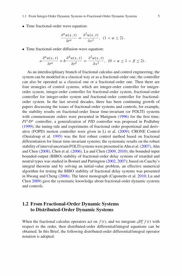
• Time fractional-order wave equation:
∂αu(x, t)
∂tα= ∂2u(x, t)
∂x2 , (1 < α ≤ 2) .
• Time fractional-order diffusion-wave equation:
a∂αu(x, t)
∂tα+ b
∂βu(x, t)
∂tβ= ∂2u(x, t)
∂x2 , (0 < α ≤ 1 < β ≤ 2) .
As an interdisciplinary branch of fractional calculus and control engineering, thesystem can be modeled in a classical way or as a fractional-order one; the controllercan also be operated as a classical one or a fractional-order one. Then there arefour strategies of control systems, which are integer-order controller for integer-order system, integer-order controller for fractional-order system, fractional-ordercontroller for integer-order system and fractional-order controller for fractional-order system. In the last several decades, there has been continuing growth ofpapers discussing the issues of fractional-order systems and controls, for example,the stability results on fractional-order linear time-invariant (or FOLTI) systemswith commensurate orders were presented in Matignon (1996) for the first time;PIλDμ controller, a generalization of PID controller was proposed in Podlubny(1999); the tuning rule and experiments of fractional order proportional and deriv-ative (FOPD) motion controller were given in Li et al. (2009); CRONE Control(Oustaloup et al. 1995) was the first robust control method based on fractionaldifferentiation for linear time-invariant systems; the systematic results on the robuststability of interval uncertain FOLTI systems were presented in Ahn et al. (2007), Ahnand Chen (2008), Chen et al. (2006), Lu and Chen (2009, 2010); the bounded-inputbounded-output (BIBO) stability of fractional-order delay systems of retarded andneutral types was studied in Bonnet and Partington (2002, 2007); based on Cauchy’sintegral theorem and by solving an initial-value problem, an effective numericalalgorithm for testing the BIBO stability of fractional delay systems was presentedin Hwang and Cheng (2006). The latest monograph (Caponetto et al. 2010; Lu andChen 2009) gave the systematic knowledge about fractional-order dynamic systemsand controls.
1.2 From Fractional-Order Dynamic Systemsto Distributed-Order Dynamic Systems
When the fractional calculus operators act on f (t), and we integrate 0Dαt f (t) with
respect to the order, then distributed-order differential/integral equations can beobtained. In this Brief, the following distributed-order differential/integral operatornotation is adopted:

6 1 Introduction
0Dw(α)t f (t) :=
∫ γ2
γ1
w(α)0Dαt f (t)dα
where w(α) denotes the weight function of distribution of order α ∈ [γ1, γ2].The idea of distributed-order equation was first proposed by Caputo (1969) and
solved by him in 1995 (Caputo 1995). The distributed-order equation is intended tomodel the input–output relationship of a linear time-invariant system based on thefrequency domain response observation, i.e., the distributed-order equation is the timedomain representation of the input–output relationship observed and constructed inthe frequency domain. The general form of the distributed-order differential equation(DODE) can be given as:
N∑i=1
ai
∫ 1
0wi (α)0Di−α
t x(t)dα +N∑
j=0
b j x ( j)(t) = f (t)
where wi (α) denotes the weight function with respect to the order α ∈ [γ1, γ2].From now on, we note that the above equation can be viewed as the generalization ofordinary differential equation (wi (α) ≡ 0) or fractional-order differential equation(wi (α) takes only discrete values in [γ1, γ2]), then it can be concluded that bothinteger-order systems and fractional-order systems are special cases of distributed-order systems (Lorenzo and Hartley 2002).
Recently, much attention has been paid to the distributed-order differentialequations and their applications in engineering fields. For example, the generalsolution of linear distributed-order differential equation was discussed systemati-cally in Bagley and Torvik (2000); distributed-order equations were introduced inthe constitutive equations of dielectric media (Caputo 1995), the distributed-orderfractional kinetics was discussed in Sokolov et al. (2004); the multi-dimensionalrandom walk models were governed by distributed fractional order differentialequations in Umarov and Steinberg (2006); particularly, the distributed-order operatorbecomes a more precise tool to explain and describe some real physical phenomenasuch as the complexity of nonlinear systems (Adams et al. 2008; Atanackovic et al.2007, 2009b, c; Diethelm and Ford 2009; Hartley and Lorenzo 2003; Lorenzo andHartley 1998, 2002; Mainardi et al. 2007a; Sokolov et al. 2004), networked struc-tures (Carlson and Halijak 1964; Lorenzo and Hartley 2002; Xu and Tan 2006),nonhomogeneous phenomena (Caputo 2001; Chen et al. 2009; Kochubei 2008;Srokowski 2008; Sun et al. 2009, 2010; Umarov and Steinberg 2006), multi-scaleand multi-spectral phenomena (Atanackovic et al. 2005; Bohannan 2000; Connolly2004; Mainardi et al. 2008; Mainardi and Pagnini 2007; Tsao 1987), etc.
Besides the distributed-order differential equations, there are still distributed-orderpartial differential equations (DOPDE) being studied as the following:
0Dw(α)t u(x, t) = ∂2
∂x2 u(x, t)

1.2 From Fractional-Order Dynamic Systems to Distributed-Order Dynamic Systems 7
where w(α) denotes the function of distribution of order α ∈ [0, 2].Let supp denotes the support set, and we can set α1 := inf {α |α ∈ supp w(α) },
and α2 := sup {α |α ∈ supp w(α) }, then the following cases can be distinguished:
• Time distributed-order diffusion-wave equation: 0 < α1 ≤ 1 < α2 ≤ 2;• Time distributed-order diffusion equation : α2 ≤ 1;• Time distributed-order wave equation : α1 > 1.
For the distributed-order partial differential equations, there have been somepapers discussing those problems. For example, the time distributed-order diffusion-wave equation was considered in Atanackovic et al. (2009b, c); time-fractionaldiffusion of distributed order was discussed in Mainardi et al. (2007b, 2008);distributed-order wave equation was analyzed in Atanackovic et al. (2011), formore knowledge about distributed-order partial differential equations, please referto Atanackovic et al. (2009a), Chechkin et al. (2002), Mainardi and Pagnini (2007),Meerschaert et al. (2011).
The theories of the distributed-order equations can be classified as: distributed-order equations (Atanackovic et al. 2009b, c; Bagley and Torvik 2000; Caputo 1995),distributed-order system identification (Hartley and Lorenzo 2003; Sokolov et al.2004; Srokowski 2008), special functions in distributed-order calculus (Atanackovicet al. 2009a; Caputo 2001; Mainardi et al. 2007a; Mainardi and Pagnini 2007),numerical methods (Chen et al. 2009; Diethelm and Ford 2009; Sun et al. 2009,2010) and so on (Atanackovic et al. 2005; Kochubei 2008). Moreover, there are alsothree surveys (Lorenzo and Hartley 1998, 2002; Umarov and Steinberg 2006) andthree thesis (Bohannan 2000; Connolly 2004; Tsao 1987) discussing the theories andapplications of distributed-order operators. It is noted that the time domain analysis ofthe distributed order operator is still unmature and urgently needed to be developed.So in this Brief, some latest results are given in Chap. 5 with several worked outexamples with MATLAB codes given in the appendices.
1.3 Preview of Chapters
In this chapter, we focus on setting up a concise context of our Brief theme bypresenting our thought on progressing from integer-order system to fractional-ordersystem, from fractional-order system to distributed-order system.
Chapter 2 is dedicated to the stability issue of distributed-order linear time-invariant (LTI) systems. Four different order distribution functions are analyzedin details. This chapter offers original and fundamental stability results for LTIdistributed-order dynamic systems (DODS). Graphical and numerical results areincluded to show the fundamental differences compared to constant order and integerorder LTI dynamic systems.
Chapter 3 serves the purpose of showing that DODS is a generalized model whichis so powerful that some really hard research problems like stability of noncommen-surate order LTI systems can be readily answered. Specifically, as the special cases

8 1 Introduction
of distributed-order linear time-invariant systems, the stability analysis of fractional-order systems with double noncommensurate orders and N-term noncommensurateorders are studied in Chap. 3.
Chapter 4 shows two generic application examples using distributed-orderoperator: distributed-order signal processing and optimal distributed-order damping.In distributed-order signal processing, the simplest case of distributed-orderintegrator/differentiator is discussed first followed by the discussion of distributed-order low-pass filter. Then, optimal distributed-order damping strategies are given fora given standard form of second order system knows as distributed-order fractionalmass-spring viscoelastic damper system. Frequency-domain method based optimalfractional-order damping systems are numerically solved.
In Chap. 5, a new general approach to discretization of distributed-order deriv-atives and integrals and to numerical solution of ordinary and partial differentialequations of distributed order is presented.
In Chap. 6, future topics related to distributed-order operator are discussed.More than 100 reference are listed and cited in this Brief, even if it can not be
a complete bibliography for this field of interest. Readers can find other referencerelated to this emerging topic.
MATLAB codes are provided as appendices so that the presented results of thisBrief are reproducible, minimizing the repetitive coding work for beginners whodecide to dive into this exciting and promising field of basic and applied researchwhich is full of opportunities of transformative research. Anyway, distributed-orderoperator, is in fact characterizing mixed-scale dynamics, or trans-scale, or cross-scaledynamics as we see it.
1.4 Chapter Summary
In this chapter we have introduced the progression from integer-order dynamicsystems to fractional-order dynamic systems, and from fractional-order dynamicsystems to distributed-order dynamic systems. Basic notations together with liter-ature reviews are presented. A brief chapter preview is included as well.
References
Adams JL, Hartley TT, Lorenzo CF (2008) Identification of complex order-distributions. J VibControl 14(9–10):1375–1388
Ahn HS, Chen YQ (2008) Necessary and sufficient stability condition of fractional-order intervallinear systems. Automatica 44(11):2985–2988
Ahn HS, Chen YQ, Podlubny I (2007) Robust stability test of a class of linear time-invariant intervalfractional-order systems using Lyapunov inequality. Appl Math Comput 187(1):27–34
Astrom KJ, Murray RM (2008) Feedback systems: an introduction for scientists and engineers.Princeton University Press, Princeton

References 9
Atanackovic TM, Budincevic M, Pilipovic S (2005) On a fractional distributed-order oscillator.J Phys A: Math Gen 38(30):6703–6713
Atanackovic TM, Oparnica L, Pilipovic S (2007) On a nonlinear distributed order fractionaldifferential equation. J Math Anal Appl 328(1):590–608
Atanackovic TM, Pilipovic S, Zorica D (2009a) Existence and calculation of the solution to thetime distributed order diffusion equation. Phys Scripta T136:014012 (6pp)
Atanackovic TM, Pilipovic S, Zorica D (2009b) Time distributed-order diffusion-wave equation.I. Volterra-type equation. Proc Royal Soc A 465:1869–1891
Atanackovic TM, Pilipovic S, Zorica D (2009c) Time distributed-order diffusion-wave equation.II. Applications of Laplace and Fourier transformations. Proc Royal Soc A 465:1893–1917
Atanackovic TM, Pilipovic S, Zorica D (2011) Distributed-order fractional wave equation on afinite domain stress relaxation in a rod. Int J Eng Sci 49(2):175–190
Bagley RL, Torvik PJ (1984) On the appearance of the fractional derivative in the behavior of realmaterials. ASME J Appl Mech 51(2):294–298
Bagley RL, Torvik PJ (2000) On the existence of the order domain and the solution of distributedorder equations (Parts I, II). Int J Appl Mech 2(7):865–882, 965–987
Bohannan G (2000) Application of fractional calculus to polarization dynamics in solid dielectricmaterials. PhD Dissertation, Montana State University, Nov 2000
Bonnet C, Partington JR (2002) Analysis of fractional delay systems of retarded and neutral type.Automatica 38(7):1133–1138
Bonnet C, Partington JR (2007) Stabilization of some fractional delay systems of neutral type.Automatica 43(12):2047–2053
Caponetto R, Dongola G, Fortuna L, Petras I (2010) Fractional order systems: modeling and controlapplications. World Scientific Company, Singapore
Caputo M (1969) Elasticità e dissipazione. Zanichelli, BolognaCaputo M (1995) Mean fractional-order-derivatives differential equations and filters. Annali
dell’Universita di Ferrara 41(1):73–84Caputo M (2001) Distributed order differential equations modelling dielectric induction and
diffusion. Fract Calc Appl Anal 4(4):421–442Carlson G, Halijak C (1964) Approximation of fractional capacitors (1/s)(1/n) by a regular Newton
process. IEEE Trans Circuit Theory 11(2):210–213Chechkin AV, Gorenflo R, Sokolov IM (2002) Retarding subdiffusion and accelerating superdif-
fusion governed by distributed-order fractional diffusion equations. Phys Rev E 66:046129Chen YQ, Ahn HS, Podlubny I (2006) Robust stability check of fractional order linear time invariant
systems with interval uncertainties. Signal Process 86(10):2611–2618Chen W, Sun HG, Zhang XD, Korosak D (2009) Anomalous diffusion modeling by fractal and
fractional derivatives. Comput Math Appl 59(5):1754–1758Connolly JA (2004) The numerical solution of fractional and distributed order differential equations.
Thesis, University of Liverpool, Dec 2004Diethelm K, Ford NJ (2009) Numerical analysis for distributed-order differential equations.
J Comput Appl Math 225(1):96–104Hartley TT, Lorenzo CF (2003) Fractional-order system identification based on continuous order-
distributions. Signal Process 83(11):2287–2300Hwang C, Cheng YC (2006) A numerical algorithm for stability testing of fractional delay systems.
Automatica 42(5):825–831Kochubei AN (2008) Distributed order calculus and equations of ultraslow diffusion. J Math Anal
Appl 340(1):252–281Li HS, Luo Y, Chen YQ (2009) A fractional order proportional and derivative (fopd) motion
controller: tuning rule and experiments. IEEE Trans Control Syst Technol 18(2):1–5Lorenzo CF, Hartley TT (1998) Initialization, conceptualization, and application in the generalized
fractional calculus. NASA technical paper, NASA/TP 1998-208415Lorenzo CF, Hartley TT (2002) Variable order and distributed order fractional operators. Nonlinear
Dyn 29(1–4):57–98
10 1 Introduction
Lu JG, Chen GR (2009) Robust stability and stabilization of fractional-order interval systems: anlmi approach. IEEE Trans Autom Control 54(6):1294–1299
Lu JG, Chen YQ (2010) Robust stability and stabilization of fractional order interval systems withthe fractional order α: The 0 < α < 1 case. IEEE Trans Autom Control 55(1):152–158
Magin RL (2006) Fractional calculus in bioengineering. Begell House, ConnecticutMainardi F, Pagnini G (2007) The role of the fox-wright functions in fractional sub-diffusion of
distributed order. J Comput Appl Math 207(2):245–257Mainardi F, Mura A, Gorenflo R, Stojanovic M (2007a) The two forms of fractional relaxation of
distributed order. J Vib Control 9:1249–1268Mainardi F, Mura A, Pagnini G, Gorenflo R (2007b) Some aspects of fractional diffusion equations
of single and distributed order. Appl Math Comput 187:295–305Mainardi F, Mura A, Pagnini G, Gorenflo R (2008) Time-fractional diffusion of distributed order.
J Vib Control 14(9–10):1267–1290Matignon D (1996) Stability results on fractional differential equations with applications to
control processing. In: Multiconference on computational engineering in systems and application,pp 963–968
Meerschaert MM, Nane E, Vellaisamy P (2011) Distributed-order fractional diffusions on boundeddomains. J Math Anal Appl 379:216–228
Miller KS, Ross B (1993) An introduction to the fractional calculus and fractional differentialequations. Wiley, New York
Oustaloup A, Mathieu B, Lanusse P (1995) The crone control of resonant plants: application to aflexible transmission. Eur J Control 1(2):113–121
Podlubny I (1999) Fractional differential equations. Academic Press, San DiegoPodlubny I (1999) Fractional-order systems and P I λ Dμ controllers. IEEE Trans Autom Control
44(1):208–214Sokolov IM, Chechkin AV, Klafter J (2004) Distributed-order fractional kinetics. Acta Phys Polonica
B 35(4):1323Srokowski T (2008) Lévy flights in nonhomogeneous media: distributed-order fractional equation
approach. Phys Rev E 78(3):031135Sun HG, Chen W, Chen YQ (2009) Variable-order fractional differential operators in anomalous
diffusion modeling. Phys A: Stat Mech Appl 388(21):4586–4592Sun HG, Chen W, Sheng H, Chen YQ (2010) On mean square displacement behaviors of anomalous
diffusions with variable and random orders. Phys Lett A 374(7):906–910Tsao YY (1987) Fractal concepts in the analysis of dispersion or relaxation processes. PhD Disser-
tation, Drexel University, June 1987Umarov S, Steinberg S (2006) Random walk models associated with distributed fractional order
differential equations. Inst Math Stat 51:117–127Xu MY, Tan WC (2006) Intermediate processes and critical phenomena: theory, method and progress
of fractional operators and their applications to modern mechanics. Sci China: Ser G Phys MechAstron 49(3):257–272

Chapter 2Distributed-Order Linear Time-InvariantSystem (DOLTIS) and Its Stability Analysis
2.1 Introduction
By using distributed-order concept, we can describe the dynamical properties of realworld system more accurately, so distributed-order system identification problem wasstudied in Hartley and Lorenzo (1999, 2003, 2004). In the following sections, thestability analysis of distributed-order linear time-invariant systems in four cases arefirst studied, then the frequency-domain responses are presented, and time-domainresponses on the basis of numerical inverse Laplace transform technique are shownin details.
2.2 Stability Analysis of DOLTIS in Four Cases
Consider a distributed-order system described by the following linear time-invariant(LTI) distributed-order differential equation (DODE) and algebraic output equation:
0Dw(α)t x(t) =
∫ 1
0w(α)0Dα
t x(t)dα = Ax(t) + Bu(t)
y(t) = Cx(t) + Du(t) (2.1)
where w(α) is the function of distribution of order α ∈ [0, 1], 0Dαt denotes the
Caputo fractional-order derivative operator, A, B, C , D are matrices with appropriatedimensions.
Remark 2.1 Since any interval (γ1, γ2) can be converted to (0, 1) through variablesubstitution, without loss of generality, the integral interval in (2.1) is considered tobe (0, 1).
Z. Jiao et al., Distributed-Order Dynamic Systems, SpringerBriefs in Control, 11Automation and Robotics, DOI: 10.1007/978-1-4471-2852-6_2,© The Author(s) 2012

12 2 Distributed-Order Linear Time-Invariant System
For the distributed-order derivative operator Dw(α)x(t), the Laplace transform is
L{
Dw(α)x(t)}
(s) = x(s)∫ 1
0w(α)sαdα − x(0)
1
s
∫ 1
0w(α)sαdα, s ∈ C\ (−∞, 0]
where x(s) = L {x(t)} (s) := ∫∞0 x(t)e−st dt . By applying the Laplace transform
to (2.1) with the assumptions that x(0) = 0, u(t) = δ(t) (δ(t) is the Dirac deltadistribution), one obtains
x(s)∫ 1
0w(α)sαdα = Ax(s) + B
i.e.,
x(s) =((∫ 1
0w(α)sαdα
)I − A
)−1
B
where I is the identity matrix. Application of the inverse Laplace transform to theprevious expression yields
x(t) = L−1
[((∫ 1
0w(α)sαdα
)I − A
)−1
B
](t), t > 0. (2.2)
In the following, four different cases of the weighting function of order are discussedrespectively.
Case 1 w(α) = 1In this case, it can be followed by (2.2) that
x(t) = L−1
[((∫ 1
0sαdα
)I − A
)−1
B
](t)
= L−1
[(s − 1
ln sI − A
)−1
B
](t)
= L−1[ln s(s I − (I + ln s A))−1 B
](t). (2.3)
Remark 2.2 It is well known from complex analysis (Asmar and Jones 2002) thatcomplex logarithm ln z = ln |z|+ i arg z (z �= 0) defines a multiple-valued function,because arg z is multiple-valued. For term ln s in (2.3), we know that it is a multi-valued function of the complex variable s whose domain can be seen as a Riemannsurface (Cuadrado and Cabanes 1989; Westerlund and Ekstam 1994) of a number ofsheets which is infinite. Note that in multiple-valued functions only the first Riemannsheet has its physical significance (Gross and Braga 1961), so we can make ln s asingle-valued function by specifying a single-valued −π < arg s < π . Because

2.2 Stability Analysis of DOLTIS in Four Cases 13
s = 0 and s on the negative real axis are nonremovable discontinuities, the branchcut of ln s is (−∞, 0].Definition 2.1 A distributed-order system H(s) defined by its impulse responseh(t) = L−1 {H(s)} is BIBO stable if and only if ∀u ∈ L∞(R+), h ∗ u ∈ L∞(R+).∗ stands for the convolution product and L∞(R+) stands for the Lebesgue space ofmeasurable function h such that ess sup
t∈R+|h(t)| < ∞.
Based on Definition 2.1 and the above analysis, the following theorem can beestablished.
Theorem 2.1 The distributed-order linear time-invariant system (2.1) with transferfunction G1(s) = C ln s(s I − (I + A ln s))−1 B + D is BIBO stable, if and only ifall the eigenvalues of A lie on the left of curve l1 := la
⋃lb in the complex plane,
where la and lb are symmetrical with respect to the real axis, and
la :={
x − iy
∣∣∣∣x = 2πω − 4 ln ω
4(ln ω)2 + π2, y = 4ω ln ω + 2π
4(ln ω)2 + π2
}
with ω ∈ [0,∞).
Proof (if part) Note that the final value theorem implies that limt→∞g(t)=sG1(s) → 0,
if all poles of sG1(s) are in the left half-plane when s → 0. It can be easily knownthat all the poles of sG1(s) satisfy the transcendental characteristic equation of theform
|(s − 1)I − A ln s| = 0. (2.4)
From (2.4) we know that s−1ln s = σi (A) (i = 1, · · · , n), where σ(A) denotes the set
of eigenvalues of A. As all the zeros of (2.4) should lie in the left half-plane to ensurethe BIBO stability of distributed-order system G1(s), it is necessary to derive therange of λ = s−1
ln s when s belongs to the left half-plane.It is natural to determine the range of λ = s−1
ln s when s lies on the imaginary axis.Then, for s = jω, (−∞ < ω < 0), we have
λ = (2π(−ω) − 4 ln(−ω)) + j (4(−ω) ln(−ω) + 2π)
4(ln(−ω))2 + π2
while for s = jω, (0 ≤ ω < ∞), we have
λ = (2πω − 4 ln ω) − j (4ω ln ω + 2π)
4(ln ω)2 + π2
which means that the imaginary axis is mapped to a curve denoted by l1, which issymmetrical with respect to the real axis. By choosing a point s randomly which lieson the left of the imaginary axis, the range of λ = s−1
ln s lies on the left of curve l1,which means that the stable region of distributed-order system (2.1) is the left region

14 2 Distributed-Order Linear Time-Invariant System
Fig. 2.1 The stable boundaryof the distributed-order system(2.1) G1(s)
0 1 2 3 4 5 6 7−20
−15
−10
−5
0
5
10
15
20
Real axis
Imag
axi
s
Fig. 2.2 The stable boundaryof the distributed-order system(2.1) G1(s) (Zoomed)
0 0.05 0.1 0.15 0.2 0.25 0.3 0.35−0.2
−0.15
−0.1
−0.05
0
0.05
0.1
0.15
0.2
Real axis
Imag
axi
s
of curve l1. In the following, l1 is plotted in Fig. 2.1, with the local property around0 zoomed in Fig. 2.2.
It can be easily known from the above analysis that if all the eigenvalues of Alie on the left of curve l1, all the poles of sG1(s) lie on the left half-plane. Fromthe final value theorem, we further know that lim
t→∞ g(t) = 0, which means the

2.2 Stability Analysis of DOLTIS in Four Cases 15
distributed-order system with transfer function G1(s) = C ln s(s I − (I + A ln s))−1
B + D is BIBO stable.(only if part) It is obviously known from Definition 2.1 that G1(s) lies in H∞,
the space of bounded analytic functions on the right half plane of the complex plane,which means that all the poles of G1(s) lie in the left half plane of the complexplane. From the proof of (if part), it is known that {sk}k=1,2,··· ,n lie in the open lefthalf plane, which is equivalents to that all the eigenvalues of A lie in the left regionwith respect to l1.
Remark 2.3 It is easy to conclude that the slope of the curve l1 at the original pointis 0, and is infinity at the infinite point, which means that any ray in the first quadrantstarts at point 0 will have point of intersection with the curve l1. This means anyconstant fractional-order approximation of DODS is problematic, since the stabilitydomains are different.
Case 2 w(α) = α
In this case, the following can be obtained under the similar analysis procedurein Case 1,
x(t) = L−1
[((∫ 1
0αsαdα
)I − A
)−1
B
]
= L−1
[(1 − s + s ln s
ln2sI − A
)−1
B
]
= L−1[
ln2s((1 − s + s ln s) I − ln2s A
)−1B
].
Theorem 2.2 The distributed-order linear time-invariant system (2.1) with
transfer function G2(s) = C ln2s((1 − s + s ln s)I − Aln2s
)−1B + D is
BIBO stable, if and only if all the eigenvalues of A lie on the left of curvel2 := lc
⋃ld , where lc and ld are symmetrical with respect to the real axis, and
lc := {x + iy |x = xω, y = yω, ω ∈ (0,∞) }, with notations
xω =(
ln ω − π2
4
) (1 − π
2 ω)− π ln ω (ω − ω ln ω)
(ln2ω + π2
4
)2
and
yω =(
ln ω − π2
4
)(ω − ω ln ω) + π ln ω
(1 − π
2 ω)
(ln2ω + π2
4
)2 .

16 2 Distributed-Order Linear Time-Invariant System
Fig. 2.3 The stable boundaryof distributed-order system(2.1) G2(s)
0 0.5 1 1.5 2−8
−6
−4
−2
0
2
4
6
8
Real axis
Imag
axi
s
Fig. 2.4 The stable boundaryof distributed-order system(2.1) G2(s) (Zoomed)
0 0.1 0.2 0.3 0.4 0.5−1
−0.8
−0.6
−0.4
−0.2
0
0.2
0.4
0.6
0.8
1
Real axis
Imag
axi
s
The proof of Theorem 2.2 can be given by the similar procedures in Theorem 2.1,the stable boundary for distributed-order system G2(s) is shown in Fig. 2.3, with thelocal property around 0 shown in Fig. 2.4.

2.2 Stability Analysis of DOLTIS in Four Cases 17
Case 3 w(α) = δ(α − β), (0 < β < 1)
In this case, the DODE (2.1) converts to a constant-order fractional-order systemdescribed by
0Dβt x(t) = Ax(t) + Bu(t)
y(t) = Cx(t) + Du(t). (2.5)
Using Laplace transform, the irrational transfer function of fractional-order system(2.5) with null initial conditions is
G3(s) = C(sβ I − A
)−1B + D. (2.6)
Remark 2.4 Note that term sβ in (2.6) defines a multi-valued function of the complexvariable s whose domain can be seen as a Riemann surface (Cuadrado and Cabanes1989; Westerlund and Ekstam 1994) of a number of sheets which is finite in thecase of β ∈ Q+, and infinite in the case of β ∈ R+\Q+. It is well known that inmultiple-valued functions only the principal sheet defined by −π < arg s < π hasits physical significance (Gross and Braga 1961).
The following can be obtained under the similar analysis procedure in the previouscases,
x(t) = L−1
[((∫ 1
0δ(α − β)sαdα
)I − A
)−1
B
](t)
= L−1[(
sβ I − A)−1
B](t).
The following theorem which corresponds to the stability condition of fractional-order system obtained in Matignon (1996) can be given.
Theorem 2.3 The fractional-order linear time-invariant system with transfer func-
tion G3(s) = C(sβ I − A
)−1B + D is BIBO stable, if and only if all the eigenvalues
of A lie on the left of curve l3 := le⋃
l f , where le and l f are symmetrical withrespect to the real axis, and le := {
reiθ∣∣r = ωβ, θ = πβ/2, ω ∈ (0,∞)
}.
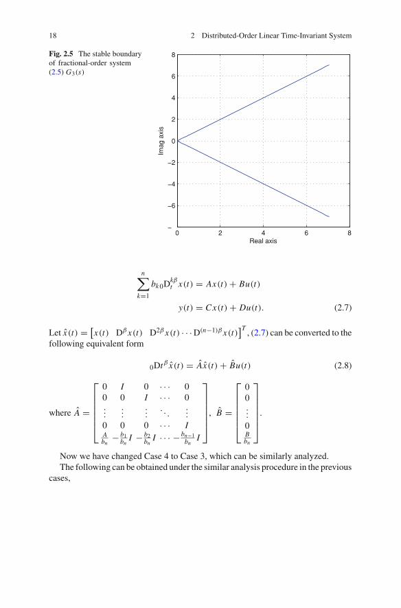
The proof of Theorem 2.3 can be given by the similar procedures in Theorem 2.1, thestable region for fractional-order system G3(s) with β = 0.5 is shown in Fig. 2.5.
Case 4 w(α) =n∑
k=1bkδ(α − kβ), (0 < nβ < 1).
In this case, the DODE (2.1) converts to the so-called LTI commensuratefractional-order system
18 2 Distributed-Order Linear Time-Invariant System
Fig. 2.5 The stable boundaryof fractional-order system(2.5) G3(s)
0 2 4 6 8−8
−6
−4
−2
0
2
4
6
8
Real axis
Imag
axi
s
n∑k=1
bk 0Dkβt x(t) = Ax(t) + Bu(t)
y(t) = Cx(t) + Du(t). (2.7)
Let x(t) = [x(t) Dβ x(t) D2β x(t) · · · D(n−1)β x(t)
]T, (2.7) can be converted to the
following equivalent form
0Dtβ x(t) = Ax(t) + Bu(t) (2.8)
where A =
⎡⎢⎢⎢⎢⎢⎣
0 I 0 · · · 00 0 I · · · 0...
......
. . ....
0 0 0 · · · IAbn
− b1bn
I − b2bn
I · · · − bn−1bn
I
⎤⎥⎥⎥⎥⎥⎦
, B =
⎡⎢⎢⎢⎢⎢⎣
00...
0Bbn
⎤⎥⎥⎥⎥⎥⎦
.
Now we have changed Case 4 to Case 3, which can be similarly analyzed.The following can be obtained under the similar analysis procedure in the previous
cases,

2.2 Stability Analysis of DOLTIS in Four Cases 19
x(t) = L−1
⎡⎣((∫ 1
0
N∑n=1
bnδ(α − βn)sαdα
)I − A
)−1
B
⎤⎦
= L−1
⎡⎣(
N∑n=1
bnsβn I − A
)−1
B
⎤⎦ .
In the following, Case 4 will not be considered.
2.3 Time-Domain Analysis: Impulse Responses
Case 1 w(α) = 1As the transfer function of distributed-order system for Case 1 with the assumption
that D = 0 is G1(s) = C ln s((s − 1)I − A ln s)−1 B, using the similar method ofimpulse response for distributed-order integrator/differentiator in Li et al. (2010),the inverse Laplace transform of G1(s) can be derived as follows.
y1(t) = L−1 {G1(s)}
= C
(1
2π i
∫ σ+i∞
σ−i∞e−st ln s(s I − (I + ln s A))−1ds
)B
= C
(∫ ∞
0e−xt (x + 1)A−1
1 dx
)B (2.9)
where A1 := ((x + 1)I + A ln x)2 + (Aπ)2.
Case 2 w(α) = α
Following the same procedures, the transfer function of distributed-order system
for Case 2 with D = 0 is G2(s) = C ln2s((s − 1 − ln s)I − Aln2s
)−1B, using the
similar method of impulse response for distributed-order integrator/differentiator inLi et al. (2010), the inverse Laplace transform of G2(s) can be derived as follows.
y2(t) = L−1{G2(s)}
= C
(1
2π i
∫ σ+i∞
σ−i∞est ln2s
((1 − s + s ln s)I − ln2s A
)−1ds
)B
= C
(∫ ∞
0e−xt
(((1 + x − x ln x) I + (
ln2x − π2)
A)2
+π2(x I + 2 ln x A)2
)A−1
2 dx
)B
(2.10)
where A2 := ((1 + x − x ln x) I + (
ln2x − π2)
A)2 + π2(x I + 2 ln x A)2.
20 2 Distributed-Order Linear Time-Invariant System
10−2 10−1 100 101 102 103−50
−40
−30
−20
−10
0
Mag
nitu
de (d
B)
10−2 10−1 100 101 102 103−80
−60
−40
−20
0
Frequency (Hz)
Pha
se (d
egre
es)
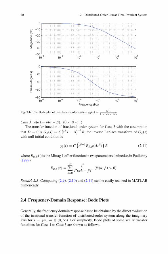
Fig. 2.6 The Bode plot of distributed-order system g2(s) = ln2s1−s+s ln s+ln2s
Case 3 w(α) = δ(α − β), (0 < β < 1)
The transfer function of fractional-order system for Case 3 with the assumptionthat D = 0 is G3(s) = C
(sβ I − A
)−1B, the inverse Laplace transform of G3(s)
with null initial condition is
y3(t) = C(
tβ−1 Eβ,β(Atβ))
B (2.11)
where Eα,β(·) is the Mittag-Leffler function in two parameters defined as in Podlubny(1999)
Eα,β(z) =∞∑
k=0
zk
Γ (αk + β), ((α, β) > 0).
Remark 2.5 Computing (2.9), (2.10) and (2.11) can be easily realized in MATLABnumerically.
2.4 Frequency-Domain Response: Bode Plots
Generally, the frequency domain response has to be obtained by the direct evaluationof the irrational transfer function of distributed-order system along the imaginaryaxis for s = jω, ω ∈ (0,∞). For simplicity, Bode plots of some scalar transferfunctions for Case 1 to Case 3 are shown as follows.

2.4 Frequency-Domain Response: Bode Plots 21
10−1
100
101
102
103
104
−60
−40
−20
0
Mag
nitu
de (
dB)
10−1
100
101
102
103
104
−50
−40
−30
−20
−10
Frequency (Hz)
Pha
se (
degr
ees)
Fig. 2.7 The Bode plot of fractional-order system g3(s) = 1s0.5+1
For w(α) = 1, the frequency-domain response of g1(s) = ln ss−1+ln s is shown in
Fig. 2.6.For w(α) = α, the frequency-domain response of g2(s) = ln2s
1−s+s ln s+ln2sis shown
in Fig. 2.7.For w(α) = δ(α − β), (0 < β < 1), the frequency-domain response of g3(s) =
1s0.5+1
is shown in Fig. 2.8.
2.5 Numerical Examples
In this section, numerical examples are shown to demonstrate the effectiveness ofthe proposed results.
Example 1 Consider a distributed-order system with Case 1 described with parame-
ters given as A =[
1 2−2 1
], B =
[11
], C = [
2 1]
and D = 0.
The eigenvalues of A are λ1 = 1 + 2 j and λ2 = 1 − 2 j , so it can be known fromTheorem 2.1 that this distributed-order system is bounded-input bounded-outputstable. Using MATLAB to derive numerically, the states of impulse response withnull initiations are shown in Figs. 2.9 and 2.10, respectively.

22 2 Distributed-Order Linear Time-Invariant System
10−1
100
101
102
103
104
−80
−60
−40
−20
0
Mag
nitu
de (
dB)
10−1
100
101
102
103
104
−100
−50
0
Frequency (Hz)
Pha
se (
degr
ees)
Fig. 2.8 The Bode plot of distributed-order system g1(s) = ln ss−1+ln s
Fig. 2.9 The state x1 of stabledistributed-order system (2.1)for Case 1
0.2 0.4 0.6 0.8 1 1.2 1.4 1.6 1.8 2−0.5
0
0.5
1
1.5
2
2.5
3
3.5
Time axis
Impu
lse
resp
onse
Example 2 Consider a distributed-order system with Case 1 described with parame-
ters given as A =[
2 2−2 2
], B =
[11
], C = [
2 1]
and D = 0.
The eigenvalues of A are λ1 = 2+2 j and λ2 = 2−2 j , and it can be known fromTheorem 2.1 that this distributed-order system is not bounded-input bounded-outputstable. Using MATLAB to derive numerically, the states of impulse response withnull initiations are shown in Figs. 2.11 and 2.12, respectively.

2.5 Numerical Examples 23
Fig. 2.10 The state x2 of sta-ble distributed-order system(2.1) for Case 1
0.2 0.4 0.6 0.8 1 1.2 1.4 1.6 1.8 2−0.5
0
0.5
1
1.5
2
2.5
3
3.5
Time axis
Impu
lse
resp
onse
Fig. 2.11 The state x1 ofunstable distributed-ordersystem (2.1) for Case 1
0 2 4 6 8 10−1000
0
1000
2000
3000
4000
5000
time axis
impu
lse
resp
onse
Example 3 Consider a distributed-order system with Case 2 described with parame-
ters given as A =[
1 3−3 1
], B =
[11
], C = [
2 1]
and D = 0.
The eigenvalues of A are λ1 = 1 + 3 j and λ2 = 1 − 3 j , so it can be known fromTheorem 2.2 that this distributed-order system is bounded-input bounded-outputstable, and the states of impulse response with null initiations are shown in Figs. 2.13and 2.14, respectively.
Example 4 Consider a distributed-order system with Case 2 described with parame-
ters given as A =[
2 2−2 2
], B =
[11
], C = [
2 1]
and D = 0.
The eigenvalues of A are λ1 = 2 + 2 j and λ2 = 2 − 2 j , it can be known fromTheorem 2.2 that this distributed-order system is not bounded-input bounded-output

24 2 Distributed-Order Linear Time-Invariant System
Fig. 2.12 The state x2 ofunstable distributed-ordersystem (2.1) for Case 1
0 2 4 6 8 10−15000
−10000
−5000
0
time axis
impu
lse
resp
onse
Fig. 2.13 The state x1 ofstable distributed-order sys-tem (2.1) for Case 2
0 5 10 15 20 25 30 35 40−2
−1.5
−1
−0.5
0
0.5
1
1.5
2
time axis
impu
lse
resp
onse
stable, and by using MATLAB to derive numerically, the states of impulse responsewith null initiations are shown in Figs. 2.15 and 2.16, respectively.
Example 5 Consider a fractional-order system for Case 3 described with parameters
given as α = 0.5, A =[
0 2−2 0
], B =
[11
], C = [
2 1]
and D = 0.
The eigenvalues of A are λ1 = 2 j and λ2 = −2 j , it can be known fromTheorem 2.3 that this fractional-order system is bounded-input bounded-output sta-ble. Using MATLAB to derive numerically, the states of impulse response with nullinitiations are shown in Figs. 2.17 and 2.18, respectively.
Example 6 Consider a fractional-order system for Case 3 described with parameters
given as α = 2/3, A =[
1 1−1 1
], B =
[11
], C = [
2 1]
and D = 0.

2.5 Numerical Examples 25
Fig. 2.14 The state x2 ofstable distributed-order sys-tem (2.1) for Case 2
0 5 10 15 20 25 30 35 40−1
−0.8
−0.6
−0.4
−0.2
0
0.2
0.4
0.6
0.8
1
time axis
impu
lse
resp
onse
Fig. 2.15 The state x1 ofunstable distributed-ordersystem (2.1) for Case 2
0 5 10 15 20−50
0
50
100
150
200
250
300
350
time axis
impu
lse
resp
onse
Since the eigenvalues of A are λ1 = 1 + j and λ2 = 1 − j , it can be known fromTheorem 2.3 that this fractional-order system is bounded-input bounded-output sta-ble. Using MATLAB to derive numerically, the states of impulse response with nullinitiations are shown in Figs. 2.19 and 2.20, respectively.
2.6 Chapter Summary
In this chapter, the bounded-input bounded-output stability conditions for four kindsof linear time-invariant distributed-order system whose integral interval being (0, 1)
have been derived for the first time. Based on the final value property of Laplacetransform, sufficient and necessary conditions of stability for distributed-order sys-

26 2 Distributed-Order Linear Time-Invariant System
Fig. 2.16 The state x2 ofunstable distributed-ordersystem (2.1) for Case 2
0 5 10 15 20−100
−80
−60
−40
−20
0
20
time axis
impu
lse
resp
onse
Fig. 2.17 The state x1 ofstable fractional-order system(2.5) for Case 3
0 2 4 6 8 10−1
0
1
2
3
4
5
Time axis
Impu
lse
resp
onse
tems are presented. In addition, time-domain and frequency-domain responses arepresented with six illustrative numerical examples. Detailed MATLAB codes areshown in Appendix A.

2.6 Chapter Summary 27
Fig. 2.18 The state x2 ofstable fractional-order system(2.5) for Case 3
0 2 4 6 8 10−1
0
1
2
3
4
5
Time axis
Impu
lse
resp
onse
Fig. 2.19 The state x1 of un-stable fractional-order system(2.5) for Case 3
0 5 10 15 20 25 30−30
−25
−20
−15
−10
−5
0
5
10
time axis
impu
lse
resp
onse

28 2 Distributed-Order Linear Time-Invariant System
Fig. 2.20 The state x2 ofunstable fractional-ordersystem (2.5) for Case 3
0 5 10 15 20 25 30−20
−10
0
10
20
30
40
time axis
impu
lse
resp
onse
References
Asmar NH, Jones GC (2002) Applied complex analysis with partial differential equations. PrenticeHall, Upper Saddle River
Cuadrado M, Cabanes R (1989) T. de Variable Compleja. Servicio de Publicaciones de la ETSITUPM, Madrid
Gross B, Braga EP (1961) Singularities of linear system functions. Elsevier, New YorkHartley TT, Lorenzo CF (1999) Fractional system identification: an approach using continuous
order-distributions. NASA Tech Memo 209640:20Hartley TT, Lorenzo CF (2003) Fractional-order system identification based on continuous order-
distributions. Signal Process 83(11):2287–2300Hartley TT, Lorenzo CF (2004) A frequency-domain approach to optimal fractional-order damping.
Nonlinear Dyn 38(1–2):69–84Li Y, Sheng H, Chen YQ (2010) On distributed order integrator/differentiator. Signal Process
91(5):1079–1084Matignon D (1996) Stability results on fractional differential equations with applications to con-
trol processing. In: Multiconference on computational engineering in systems and application,pp 963–968
Podlubny I (1999) Fractional differential equations. Academic Press, San DiegoWesterlund S, Ekstam L (1994) Capacitor theory. IEEE Trans Dielectr Electr Insul 1(5):826–839

Chapter 3Noncommensurate Constant Ordersas Special Cases of DOLTIS
3.1 Introduction
Stability is a minimum requirement for control systems, certainly including fractional-order systems. In Matignon (1996), the stability results on fractional-order lineartime-invariant (FO-LTI) systems with commensurate orders were presented for thefirst time, it permits to check the asymptotically stability through the location ofthe system matrix eigenvalues of the pseudo state space representation of fractional-order system in the Complex plane. Henceforth, there were some systematic resultson the robust stability of interval uncertain FO-LTI systems as presented in Ahn andChen (2008), Ahn et al. (2007), Chen et al. (2006), Lu and Chen (2010), Petras et al.(2004). The BIBO-stability of fractional-order delay systems of retarded and neutraltypes was studied in Bonnet and Partington (2002), in which necessary and suffi-cient conditions were presented for retarded type, and only sufficient conditions wereprovided for neutral type. In Bonnet and Partington (2007), necessary and sufficientconditions of stability were provided for an important special case fractional-orderdelay system of neutral type. However, such theorems obtained in Bonnet and Part-ington (2002, 2007) don’t permit to conclude the system stability without computingthe system’s poles, which constitutes tedious work, so based on Cauchy’s integraltheorem and by solving an initial-value problem, an effective numerical algorithmfor testing the BIBO stability of fractional delay systems was presented in Hwangand Cheng (2006).
However, the fractional-order systems discussed in these literatures are mostlywith commensurate orders, which means the orders can always converted to com-mensurate orders when they have a common divisor. To the best of our knowledge,there are few results concerning the stability analysis problems for fractional-ordersystems with noncommensurate orders. Based on Cauchy’s theorem, a graphicaltest to evaluate fractional-order systems with noncommensurate orders are given inSabatier et al. (2010), however, this method is not very helpful because of the com-plicated procedures. Therefore motivated by the previous references, this section
Z. Jiao et al., Distributed-Order Dynamic Systems, SpringerBriefs in Control, 29Automation and Robotics, DOI: 10.1007/978-1-4471-2852-6_3,© The Author(s) 2012

30 3 Noncommensurate Constant Orders as Special Cases of DOLTIS
addresses the bounded-input bounded-output stability for fractional-order systemswith multiple discrete noncommensurate orders.
3.2 Stability Analysis of Some Special Cases of DOLTIS
3.2.1 Case 1: Double Noncommensurate Orders
For the distributed-order system with double noncommensurate orders described by
0Dw(α)t x(t) =
∫ 1
0w(α)0Dα
t x(t)dα = Ax(t) + Bu(t)
y(t) = Cx(t) + Du(t), (3.1)
where 0Dαt denotes Caputo fractional-order derivative operator, w(α) = δ (α − β1)+
δ (α − β2) is the function distribution of order α ∈ [0, 1], 0 < β1, β2 ≤ 1 arenoncommensurate orders, which means that they do not have a common divisor.
Remark 3.1 When the function distribution of order takes discrete values, distributed-order system (3.1) will be fractional-order system with double noncommensu-rate orders. Fractional-order system (3.1) can always be converted to a fractional-order system with commensurate orders if both β1 and β2 are rational numbers(Monje et al. 2010), and the stability issue of fractional-order system with com-mensurate orders has been solved in Matignon (1996). When at least one of β1 andβ2 is not a rational number, or β1 and β2 are not commensurate numbers, they donot have common divisors. Based on Cauchy’s theorem, a graphical test to evaluatefractional-order systems with noncommensurate orders are given in Sabatier et al.(2010), and the system is considered in frequency domain, however, this method isnot very helpful because of the complicated procedures. In current section, sufficientand necessary condition for fractional-order system with double noncommensurateorders is proposed first.
Under the assumption of zero initial conditions, taking the Laplace transform of(3.1), we have
sβ1 X (s) + sβ2 X (s) = AX (s) + BU (s).
Assume that D = 0. The transfer function of (3.1) is
H(s) = C((sβ1 + sβ2)I − A
)−1B.
Similar to the BIBO stability for traditional control systems, we have the followingdefinition.
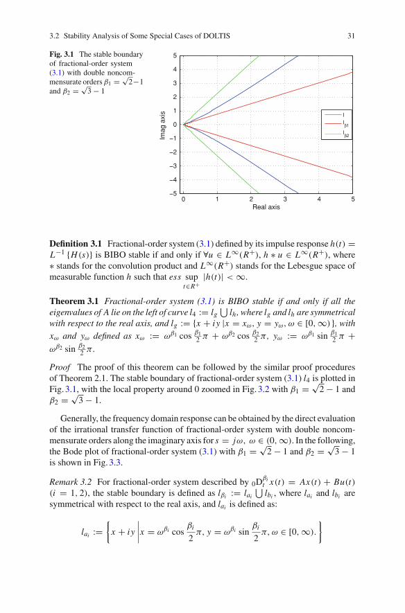
3.2 Stability Analysis of Some Special Cases of DOLTIS 31
Fig. 3.1 The stable boundaryof fractional-order system(3.1) with double noncom-mensurate orders β1 = √
2−1and β2 = √
3 − 1
0 1 2 3 4 5−5
−4
−3
−2
−1
0
1
2
3
4
5
Real axis
Imag
axi
s
llβ1
lβ2
Definition 3.1 Fractional-order system (3.1) defined by its impulse response h(t) =L−1 {H(s)} is BIBO stable if and only if ∀u ∈ L∞(R+), h ∗ u ∈ L∞(R+), where∗ stands for the convolution product and L∞(R+) stands for the Lebesgue space ofmeasurable function h such that ess sup
t∈R+|h(t)| < ∞.
Theorem 3.1 Fractional-order system (3.1) is BIBO stable if and only if all theeigenvalues of A lie on the left of curve l4 := lg
⋃lh , where lg and lh are symmetrical
with respect to the real axis, and lg := {x + iy |x = xω, y = yω, ω ∈ [0,∞) }, withxω and yω defined as xω := ωβ1 cos β1
2 π + ωβ2 cos β22 π , yω := ωβ1 sin β1
2 π +ωβ2 sin β2
2 π .
Proof The proof of this theorem can be followed by the similar proof proceduresof Theorem 2.1. The stable boundary of fractional-order system (3.1) l4 is plotted inFig. 3.1, with the local property around 0 zoomed in Fig. 3.2 with β1 = √
2 − 1 andβ2 = √
3 − 1.
Generally, the frequency domain response can be obtained by the direct evaluationof the irrational transfer function of fractional-order system with double noncom-mensurate orders along the imaginary axis for s = jω, ω ∈ (0,∞). In the following,the Bode plot of fractional-order system (3.1) with β1 = √
2 − 1 and β2 = √3 − 1
is shown in Fig. 3.3.
Remark 3.2 For fractional-order system described by 0Dβit x(t) = Ax(t) + Bu(t)
(i = 1, 2), the stable boundary is defined as lβi := lai
⋃lbi , where lai and lbi are
symmetrical with respect to the real axis, and lai is defined as:
lai :={
x + iy
∣∣∣∣x = ωβi cosβi
2π, y = ωβi sin
βi
2π,ω ∈ [0,∞).
}

32 3 Noncommensurate Constant Orders as Special Cases of DOLTIS
Fig. 3.2 The stable boundaryof fractional-order system(3.1) with double noncom-mensurate orders β1 = √
2−1and β2 = √
3 − 1 (Zoomed)
0 0.1 0.2 0.3 0.4 0.5−0.5
−0.4
−0.3
−0.2
−0.1
0
0.1
0.2
0.3
0.4
0.5
Imag
axi
s
llβ1
lβ2
Fig. 3.3 The bode plot offractional-order system (3.1)with double noncommensu-rate orders β1 = √
2 − 1 andβ2 = √
3 − 1
10−1 100 101 102 103 104−60
−40
−20
0
Mag
nitu
de (
dB)
10−1 100 101 102 103 104−80
−60
−40
−20
Frequency (Hz)
Pha
se (
degr
ees)
lβ1 and lβ2 are also plotted in Figs. 3.1 and 3.2. It can be easily seen from Figs. 3.1and 3.2 that curve l lies between lβ1 and lβ2 .
Remark 3.3 We assume that 0 < β1, β2 ≤ 1 in (3.1), which means that bothβ1 and β2 cannot be 0. Without loss of generality, if β2 = 0, β1 is an irrationalnumber, fractional-order system (3.1) will become 0Dβ1
t x(t) = Ax(t)+ Bu(t), withA = A− I . In this case, the stable boundary is lβ1 defined in Remark 3.2 with respectto A.
Remark 3.4 If both β1 and β2 are irrational numbers. Let β2 = kβ1, where k is apositive integer. Here it means that the orders are commensurate orders, then thefollowing cases can be easily given:

3.2 Stability Analysis of Some Special Cases of DOLTIS 33
• If k = 1, fractional-order system (3.1) will become 20Dβ1t x(t) = Ax(t) + Bu(t),
i.e., 0Dβ1t x(t) = A1x(t) + B1u(t), with A1 = A/2, B1 = B/2, and the stable
boundary is lβ1 defined in Remark 3.2 with respect to A1.
• If k = 2, fractional-order system (3.1) will become 0D2β1t x(t) + 0Dβ1
t x(t) =Ax(t)+Bu(t). Let x(t) :=
[x(t) 0Dβ1
t x(t)]T
, then we have Dβ1 x(t) = A2 x(t)+B2u(t), with A2 =
[ 0 IA −I
], B2 =
[ 0B
], and the stable boundary is lβ1 defined
in Remark 3.2 with respect to A2.• If k is any positive integer, the similar conclusion can be obtained.
3.2.2 Case 2: N-Term Noncommensurate Orders
For the fractional-order system with N -term noncommensurate orders described by
0Dw(α)t x(t) =
∫ 1
0w(α)0Dα
t x(t)dα = Ax(t) + Bu(t)
y(t) = Cx(t) + Du(t) (3.2)
where 0Dαt denotes Caputo fractional-order derivative operator, w(α)=
n∑i=1
δ(α − βi )
is the function distribution of order α ∈ [0, 1], 0 < β1, β2, · · · , βn ≤ 1 are N -termnoncommensurate orders, which means that they do not have a common divisor.
Similar to the analysis in Case 1, let u(t) = δ(t), then the transfer function of(3.2) under the assumption of zero initial conditions is
H1(s) = C
(n∑
i=1
sβi I − A
)−1
B.
We have the following parallel result.
Theorem 3.2 Fractional-order system (3.2) is BIBO stable if and only if all theeigenvalues of A lie on the left of curve l5 := li
⋃l j , where li and l j are symmetrical
with respect to the real axis, and li is defined as:
li := {x + iy |x = xω, y = yω, ω ∈ (0,∞) }
with xω and yω defined as xω :=n∑
i=1ωβi cos βi
2 π , yω :=n∑
i=1ωβi sin βi
2 π .
Proof The proof of this theorem is similar to the proof of Theorem 2.1.
34 3 Noncommensurate Constant Orders as Special Cases of DOLTIS
Fig. 3.4 The state x1 of stablefractional-order system (3.1)with double noncommensu-rate orders β1 = √
2 − 1 andβ2 = √
3 − 1
0 2 4 6 8 10−1
0
1
2
3
4
5
6
7
time axis
impu
lse
resp
onse
NILTImpulse response invariant Discrete approximated
Remark 3.5 From the calculation and plots through MATLAB in Case 1, it can beknown that curve l5 must lies between lmin and lmax which are defined as
lmin :={
reiθ∣∣∣∣θ = ±min {βi }
2π, r ≥ 0
}
and
lmax :={
reiθ∣∣∣∣θ = ±max {βi }
2π, r ≥ 0
}.
3.3 Numerical Examples
In this section, numerical examples are presented to demonstrate the effectivenessof the proposed concept.
Example 1 Consider a fractional-order system (3.1) with double noncommensurate
orders described with parameters β1 = √2 − 1, β2 = √
3 − 1, A =[
1 2−2 1
],
B =[
11
], C = [
2 1]
and D = 0.
The eigenvalues of A are λ1 = 1 + 2 j and λ2 = 1 − 2 j , and it can beknown from Theorem 3.1 that this fractional-order system is bounded-input bounded-output stable. Based on the numerical inverse Laplace transform (NILT) technique(Li et al. 2011), the states of impulse response for Gd1(s)=C
((sβ1 + sβ2)I − A
)−1B
with null initiations are shown in Figs. 3.4 and 3.5, respectively.

3.3 Numerical Examples 35
Fig. 3.5 The state x2 of stablefractional-order system (3.1)with double noncommensu-rate orders β1 = √
2 − 1 andβ2 = √
3 − 1
0 2 4 6 8 10−1
0
1
2
3
4
5
6
7
time axis
impu
lse
resp
onse
NILTImpulse response invariant Discrete approximated
Fig. 3.6 The state x1 ofunstable fractional-ordersystem (3.1) with doublenoncommensurate ordersβ1 = √
2−1 and β2 = √3−1
0 2 4 6 8 10−2
−1.5
−1
−0.5
0
0.5
1
1.5
2
2.5
3
time axis
impu
lse
resp
onse
Example 2 Consider a fractional-order system (3.1) with double noncommensurate
orders described with parameters β1 = √2 − 1, β2 = √
3 − 1, A =[
1 1−1 1
],
B =[
11
], C = [
2 1]
and D = 0.
The eigenvalues of A are λ1 = 1 + j and λ2 = 1 − j , so it can be knownfrom Theorem 3.1 that this fractional-order system is not bounded-input bounded-output stable. Based on the NILT technique, the states of impulse response forGd2 = C
((sβ1 + sβ2)I − A
)−1B with null initiations are shown in Figs. 3.6 and
3.7, respectively.

36 3 Noncommensurate Constant Orders as Special Cases of DOLTIS
Fig. 3.7 The state x2 ofunstable fractional-ordersystem (3.1) with doublenoncommensurate ordersβ1 = √
2−1 and β2 = √3−1
0 2 4 6 8 10−2
−1.5
−1
−0.5
0
0.5
1
1.5
2
2.5
3
time axis
impu
lse
resp
onse
3.4 Chapter Summary
In this chapter, the stability issues for fractional-order linear time-invariant systemswith multiple noncommensurate orders are solved. The double noncommensurateorders and N -term noncommensurate orders are analyzed respectively and sufficientand necessary conditions of stability are obtained. In addition, based on the nu-merical inverse Laplace transform technique, time-domain responses for the doublenoncommensurate order case are presented to verify the main results as illustrativenumerical examples. Detailed MATLAB codes are presented in Appendix A.
References
Ahn HS, Chen YQ (2008) Necessary and sufficient stability condition of fractional-order intervallinear systems. Automatica 44(11):2985–2988
Ahn HS, Chen YQ, Podlubny I (2007) Robust stability test of a class of linear time-invariant intervalfractional-order systems using Lyapunov inequality. Appl Math Comput 187(1):27–34
Bonnet C, Partington JR (2002) Analysis of fractional delay systems of retarded and neutral type.Automatica 38(7):1133–1138
Bonnet C, Partington JR (2007) Stabilization of some fractional delay systems of neutral type.Automatica 43(12):2047–2053
Chen YQ, Ahn HS, Podlubny I (2006) Robust stability check of fractional order linear time invariantsystems with interval uncertainties. Signal Process 86(10):2611–2618
Hwang C, Cheng YC (2006) A numerical algorithm for stability testing of fractional delay systems.Automatica 42(5):825–831
Li Y, Sheng H, Chen YQ (2011) Analytical impulse response of a fractional second order filter andits impulse response invariant discretization. Signal Process 91(3):498–507
Lu JG, Chen YQ (2010) Robust stability and stabilization of fractional order interval systems withthe fractional order α: the 0 < α < 1 case. IEEE Trans Autom Control 55(1):152–158

References 37
Matignon D (1996) Stability results on fractional differential equations with applications to con-trol processing. In: Multiconference on computational engineering in systems and application,pp 963–968
Monje CA, Chen YQ, Vinagre BM, Xue DY, Feliu V (2010) Fractional-order systems and controls:fundamentals and applications. Springer, London
Petras I, Chen YQ, Vinagre BM, Podlubny I (2004) Stability of linear time invariant systems withinterval fractional orders and interval coefficients. In: Proceedings of the international conferenceon computational cybernetics, pp 341–346
Sabatier J, Farges C, Trigeassou JC (2010) A stability test for non commensurate fractional ordersystem. In: Proceedings of the 4th IFAC workshop on fractional differentiation and its applications
Chapter 4Distributed-Order Filtering andDistributed-Order Optimal Damping
The idea of using the distributed-order differential equation first proposed by Caputo(1969) is at least mathematically interesting as demonstrated in the previous chapters.However, people may question its usefulness in engineering practice. In this chapter,we included two generic applications. One is on distributed order signal processingand the other is on optimal distributed damping. We hope these two initial applicationscan serve as motivating examples to further the investigation in distributed orderdynamics systems, signal processing, modeling and controls.
4.1 Application I: Distributed-Order Filtering
Filtering as a special type of dynamic system is a signal processing technique.In this section, we present two distributed-order filters: the distributed-orderintegrator/differentiator and the distributed-order low-pass filter. These twodistributed order filters are studied in both time domain and frequency domain.Moreover, the discretization method is used to obtain the digital impulse responsesof these distributed-order fractional filters. The results are verified in both time andfrequency domains.
4.1.1 Distributed-Order Integrator/Differentiator
Motivated by the applications of the distributed-order operators in control, filteringand signal processing, a distributed-order integrator/differentiator is derived step bystep in this section. Firstly, the classical integer order integrator can be rewritten as
1
s=
∫ ∞
−∞δ(α − 1)
1
sαdα, (4.1)
Z. Jiao et al., Distributed-Order Dynamic Systems, SpringerBriefs in Control, 39Automation and Robotics, DOI: 10.1007/978-1-4471-2852-6_4,© The Author(s) 2012

40 4 Distributed-Order Filtering
where δ(·) denotes the Dirac–Delta function and 1sα is the fractional-order integrator/
differentiator with order α ∈ R. Moreover, the summation of a series of fractional-order integrators/differentiators can be expressed as
∑k
1
sαk=
∫ ∞
−∞
[∑k
δ(α − αk)
]1
sαdα, (4.2)
where k can belong to any countable or noncountable set. Now, it is straightforward
to replace
[∑k
δ(α − αk)
]by a weighted kernel function w(α). It follows that the
right side of the above equation becomes
∫ ∞
−∞w(α)
1
sαdα, (4.3)
where w(α) is independent of time, and the above equation defines a distributed-orderintegrator/differentiator. Particularly, when w(α) is a piecewise function,
∫ ∞
−∞w(α)
1
sαdα = w(αl)
∫ bl
al
1
sαdα, (4.4)
where al , bl are real numbers, αl ∈ (al , bl) and w(α) is a constant on α ∈ (al , bl).Based on the above discussions, without loss of generality, we focus on the uniformdistributed-order integrator/differentiator
∫ ba
1sα dα, where a < b are arbitrary real
numbers.In order to apply the distributed-order integrator/differentiator, the numerical
discretization method is needed. This finds applications in signal modeling, filterdesign, controller design (Machado 1997) and nonlinear system identification(Hartley and Lorenzo 2003; Adams et al. 2008). The numerical discretization of thedistributed-order integrator/differentiator, the key step towards application, can berealized in two ways: direct methods and indirect methods. In indirect discretizationmethods (Oustaloup et al. 2000; Chen and Moore 2002), two steps are required, i.e.,frequency domain fitting in continuous time domain first and then discretizing the fits-transfer function (Chen and Moore 2002). Other frequency-domain fitting methodscan also be used but without guaranteeing the stable minimum-phase discretization(Chen and Moore 2002). In this section, the direct discretization method will be usedby an effective impulse response invariant discretization method discussed in Chenand Moore (2002), Chen and Vinagre (2003), Lubich (1986), Chen et al. (2004),and Li et al. (2011). In the above-mentioned references, the authors developed atechnique for designing the discrete-time IIR filters from continuous-time fractional-order filters, in which the impulse response of the continuous-time fractional-order filter is sampled to produce the impulse response of the discrete-time filter.The detailed techniques of the impulse response invariant discretization method willbe introduced in Sect. 4.1.1.2. For more discussions of the discretization methods,

4.1 Application I: Distributed-Order Filtering 41
we cite Vinagre et al. (2003), Barbosa and Machado (2006), Ferdi (2009), Oustaloup(1981) and Radwan et al. (2007, 2008).
4.1.1.1 Impulse Response of the Distributed-OrderIntegrator/Differentiator
For the distributed-order integrator/differentiator (DOI/D)
∫ b
a
1
sαdα = s−a − s−b
ln(s), (4.5)
where a < b are arbitrary real numbers, its inverse Laplace transform is written as
L−1{∫ b
a
1
sαdα
}= 1
2π i
∫ σ+i∞
σ−i∞est s−a − s−b
ln(s)ds, (4.6)
where σ > 0. It can be seen that there are two branch points of (4.5), s = 0 ands = ∞. Therefore, we can cut the complex plane by connecting the branch pointsalong the negative real domain, so that the path integral in (4.6) is equivalent to thepath integral along the Hankel path.1 The Hankel path starts from −∞ along lowerside of real (horizontal) axis, encircles the circular disc |s| = ε → 0, in the positivesense, and ends at −∞ along the upper side of real axis. Moreover, it can also be
proved that the path integral of est (s−a−s−b)ln(s) along s → 0 equals zero for b ≤ 1, and
that there are no poles in the single value analytical plane. Therefore, by substitutings = −xe−iπ and s = xeiπ , where x ∈ (0,+∞), we have, for an arbitrary σ > 0and b ≤ 1,
L−1{∫ b
a
1
sαdα
}= 1
2π i
∫ σ+i∞
σ−i∞est
(s−a − s−b
)ln(s)
ds
= 1
2π i
∫ ∞
0
e−xt(x−aeaπ i − x−bebπ i
)ln(x) − iπ
dx
− 1
2π i
∫ ∞
0
e−xt(x−ae−aπ i − x−be−bπ i
)ln(x) + iπ
dx
= 1
π
∫ ∞
0
e−xt
(ln(x))2 + π2
[x−a(sin(aπ) ln(x) + π cos(aπ))
−x−b(sin(bπ) ln(x) + π cos(bπ))]
dx . (4.7)
Based on the above discussions, we arrive at the following theorem.
1 It follows from the residue of est (s−a−s−b)ln(s) which equals zero at s = ∞, that the path integral of it
along s → ∞ is vanished for b ≤ 1.

42 4 Distributed-Order Filtering
Theorem 4.1 For any a < b ≤ 1, we have
L−1{∫ b
a
1
sαdα
}= 1
π
∫ ∞
0
e−xt
(ln(x))2 + π2
[x−a(sin(aπ) ln(x) + π cos(aπ))
− x−b(sin(bπ) ln(x) + π cos(bπ))]dx . (4.8)
Especially, when 0 ≤ a < b ≤ 1, it can be derived that
∣∣∣∣L−1{∫ b
a
1
sαdα
}∣∣∣∣ ≤ 1
π2
(M1ta−1
|a − 1| + M2tb−1
|b − 1|)
, (4.9)
where M1 and M2 are finite positive constants.
Proof The first equation in this theorem is the same as (4.7). Moreover, by using(4.7), it can be easily proved that
∣∣∣∣L−1{∫ b
a
1
sαdα
}∣∣∣∣ ≤ 1
π2
∫ ∞
0e−xt (x−a + x−b)dx = 1
π2
(M1ta−1
|a − 1| + M2tb−1
|b − 1|)
,
where M1 = ∫ ∞0 e−τ 1/(1−a)
dτ and M2 = ∫ ∞0 e−τ 1/(1−b)
dτ are finite positive constantsfor any 0 ≤ a < b ≤ 1.
Based on the above discussions we can get the time domain expression of the impulseresponse of the distributed-order integrator/differentiator for any a < b ≤ 1. Notehere, for a < b ≤ 1, (4.7) can be easily computed by using “quadgk” in MATLAB®,which will be used in the discretization method. Moreover, in order to extend a andb to the whole real axis, we can use the following properties.
Property 4.1 It can be proved that
(A) sc∫ b
a1sα dα = ∫ b−c
a−c1sα dα, where c ∈ R.
(B)∫ b
a1sα dα = s
∫ 1a+1
1sα dα + ∫ b
01sα dα, where a ∈ [−1, 0) and b ∈ [0, 1].
(C)∫ b
a1sα dα = (s−1 +· · ·+ s−N )s−[a] ∫ a−[a]
a−[a]−11sα dα + s−(N+[a]+1) ·∫ b−(N+[a]+1)
a−[a]−11sα dα, where b − a > 1, N = [b − a] and [∗] denotes the integer part of ∗.
(D)∫ b
a sαdα = s∫ b
a1sα dα, where a < b, a = 1 − b and b = 1 − a.
(E) The distributed integrator/differentiator∫ b
aw(α)
sα dα, where w(α) is a piecewisefunction, can be converted to the summation of uniformly distributed integrators/differentiators.
Theorem 4.2 Any distributed-order integrator/differentiator can be composed bythe distributed-order integrator for 0 ≤ a < b ≤ 1, integrator 1
s and differentiator s.
Proof This theorem can be proved by Property 4.1.

4.1 Application I: Distributed-Order Filtering 43
0.1 0.2 0.3 0.4 0.5 0.6 0.7 0.8 0.9 10
0.2
0.4
0.6
0.8
1
Time
Impu
lse
Res
pons
e
impulse response of ∫abs−αdα
approximated impulse response
Fig. 4.1 The impulse responses of the approximate discrete-time IIR filter and the continuous-timedistributed-order filter when a = 0.6, b = 1 and Ts = 0.001 s
4.1.1.2 Impulse Response Invariant Discretization of DOI/DOD
The impulse response invariant discretization method converts analog filter transferfunctions to digital filter transfer function in such a way that the impulse responsesare the same (invariant) at the sampling instants. Thus, if g(t) denotes the impulse-response of an analog (continuous-time) filter, then the digital (discrete-time) filtergiven by the impulse-invariant method will have impulse response g(nTs), where Ts
denotes the sampling period in seconds.Impulse response invariance-based IIR-type discretization method is a simple
and efficient numerical discretization method for the approximation of fractional-order filter (Chen 2003, 2008a, b; Chen and Vinagre 2003). The method not onlycan accurately approximate the fractional-order filter in time domain but also fit thefrequency response very well in the low frequency band in the frequency domain(Li et al. 2010a). Figures 4.1 and 4.2 show the impulse responses and the frequencyresponse of the approximated discrete-time IIR filter and the continuous-timefractional-order filter when a = 0.6, b = 1 and Ts = 0.001 s, respectively. Thetransfer function of the approximated IIR filter is
0.00167 − 0.006112z−1 + 0.008409z−2 − 0.005208z−3 + 0.00129z−4 − 4.785 · 10−5z−5
1 − 4.488z−1 + 8.004z−2 − 7.082z−3 + 3.104z−4 − 0.5383z−5.
(4.10)
For frequency response, the impulse response invariant discretization methodworks well for the band-limited (1–100 Hz) continuous-time fractional-order filters.This figure is plotted by the MATLAB code (Sheng 2010), where we used theMATLAB command [sr] = irid_doi(0.001,0.6, 1,5, 5).
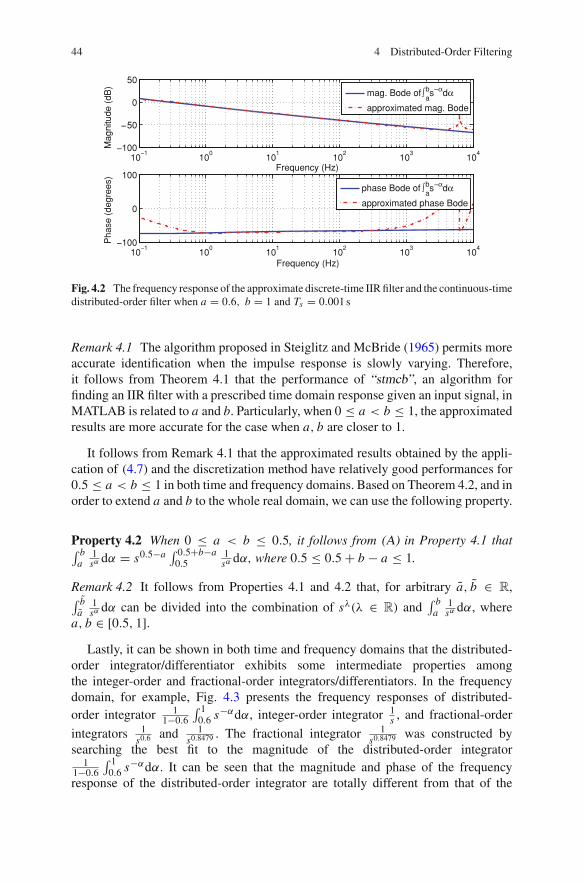
44 4 Distributed-Order Filtering
10−1
100
101
102
103
104
−100
−50
0
50
Frequency (Hz)
Mag
nitu
de (
dB)
mag. Bode of ∫abs−αdα
approximated mag. Bode
10−1
100
101
102
103
104
−100
0
100
Frequency (Hz)
Pha
se (
degr
ees)
phase Bode of ∫abs−αdα
approximated phase Bode
Fig. 4.2 The frequency response of the approximate discrete-time IIR filter and the continuous-timedistributed-order filter when a = 0.6, b = 1 and Ts = 0.001 s
Remark 4.1 The algorithm proposed in Steiglitz and McBride (1965) permits moreaccurate identification when the impulse response is slowly varying. Therefore,it follows from Theorem 4.1 that the performance of “stmcb”, an algorithm forfinding an IIR filter with a prescribed time domain response given an input signal, inMATLAB is related to a and b. Particularly, when 0 ≤ a < b ≤ 1, the approximatedresults are more accurate for the case when a, b are closer to 1.
It follows from Remark 4.1 that the approximated results obtained by the appli-cation of (4.7) and the discretization method have relatively good performances for0.5 ≤ a < b ≤ 1 in both time and frequency domains. Based on Theorem 4.2, and inorder to extend a and b to the whole real domain, we can use the following property.
Property 4.2 When 0 ≤ a < b ≤ 0.5, it follows from (A) in Property 4.1 that∫ ba
1sα dα = s0.5−a
∫ 0.5+b−a0.5
1sα dα, where 0.5 ≤ 0.5 + b − a ≤ 1.
Remark 4.2 It follows from Properties 4.1 and 4.2 that, for arbitrary a, b ∈ R,∫ ba
1sα dα can be divided into the combination of sλ(λ ∈ R) and
∫ ba
1sα dα, where
a, b ∈ [0.5, 1].Lastly, it can be shown in both time and frequency domains that the distributed-
order integrator/differentiator exhibits some intermediate properties amongthe integer-order and fractional-order integrators/differentiators. In the frequencydomain, for example, Fig. 4.3 presents the frequency responses of distributed-order integrator 1
1−0.6
∫ 10.6 s−αdα, integer-order integrator 1
s , and fractional-order
integrators 1s0.6 and 1
s0.8479 . The fractional integrator 1s0.8479 was constructed by
searching the best fit to the magnitude of the distributed-order integrator1
1−0.6
∫ 10.6 s−αdα. It can be seen that the magnitude and phase of the frequency
response of the distributed-order integrator are totally different from that of the
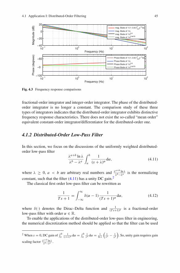
4.1 Application I: Distributed-Order Filtering 45
10−1
100
101
102
−40
−20
0
20
Frequency (Hz)
Mag
nitu
de (
dB)
10−1
100
101
102
−100
−80
−60
Frequency (Hz)
Pha
se (
degr
ees)
Phase Bode of 1/(1−0.6)*∫0.61 s−αdα
Phase Bode of 1/s
Phase Bode of 1/s0.6
Phase Bode of 1/s0.8479
mag. Bode of 1/(1−0.6)*∫0.61 s−αdα
mag. Bode of 1/s
mag. Bode of 1/s0.6
mag. Bode of 1/s0.8479
Fig. 4.3 Frequency response comparisons
fractional-order integrator and integer-order integrator. The phase of the distributed-order integrator is no longer a constant. The comparison study of these threetypes of integrators indicates that the distributed-order integrator exhibits distinctivefrequency response characteristics. There does not exist the so-called “mean order”equivalent constant-order integrator/differentiator for the distributed-order one.
4.1.2 Distributed-Order Low-Pass Filter
In this section, we focus on the discussions of the uniformly weighted distributed-order low-pass filter
λa+b ln λ
λb − λa
∫ b
a
1
(s + λ)αdα, (4.11)
where λ ≥ 0, a < b are arbitrary real numbers and λa+b ln λλb−λa is the normalizing
constant, such that the filter (4.11) has a unity DC gain.2
The classical first order low-pass filter can be rewritten as
1
T s + 1=
∫ ∞
−∞δ(α − 1)
1
(T s + 1)αdα, (4.12)
where δ(·) denotes the Dirac–Delta function and 1(T s+1)α
is a fractional-orderlow-pass filter with order α ∈ R.
To enable the applications of the distributed-order low-pass filter in engineering,the numerical discretization method should be applied so that the filter can be used
2 When s = 0, DC gain of∫ b
a1
(s+λ)αdα = ∫ b
a1λα dα = 1
ln λ
(1λa − 1
λb
). So, unity gain requires gain
scaling factor λa+b ln λλb−λa .
46 4 Distributed-Order Filtering
in signal modeling, filter design and nonlinear system identification (Hartley andLorenzo 2003; Adams et al. 2008; Li et al. 2010b). Let us first derive the analyticalform of the filter’s impulse response.
4.1.2.1 Impulse Response of the Distributed-Order Low-Pass Filter
In this section the analytical form of
L−1{∫ b
a
1
(s + λ)αdα
}(4.13)
is derived and is in a computable form in MATLAB. This will be used in the impulseresponse invariant discretization in the next section.
It follows from the properties of inverse Laplace transform that
L−1{∫ b
a
1
(s + λ)αdα
}= e−λtL−1
{∫ b
a
1
(sα)dα
}. (4.14)
It has been provided that by substituting s = −xe−iπ and s = xeiπ , where x ∈(0,+∞), we have, for an arbitrary σ > 0 and b ≤ 1,
L−1{∫ b
a
1
sαdα
}= 1
π
∫ ∞
0
e−xt
(ln(x))2 + π2
[x−a(sin(aπ) ln(x) + π cos(aπ))
− x−b(sin(bπ) ln(x) + π cos(bπ))]dx . (4.15)
Theorem 4.3 For any a, b ∈ R, we have
∣∣∣∣L−1{∫ b
a
1
(s + λ)αdα
}∣∣∣∣ ≤ e−λt
π2
(M1ta−1
|a − 1| + M2tb−1
|b − 1|)
,
where M1 and M2 are finite positive constants.
Proof By using (4.15), it can be easily proved that
∣∣∣∣L−1{∫ b
a
1
(s + λ)αdα
}∣∣∣∣ ≤ e−λt
π2
∫ ∞
0e−xt (x−a + x−b)dx
= e−λt
π2
(M1ta−1
|a − 1| + M2tb−1
|b − 1|)
,

4.1 Application I: Distributed-Order Filtering 47
Fig. 4.4 The impulseresponse of 1
0.4
∫ 10.6
1(s+1)α
dα
0.1 0.2 0.3 0.4 0.5 0.6 0.7 0.8 0.90
1
2
3
4
5
TimeIm
puls
e re
spon
se
. .
where M1=∫ ∞
0 e−τ 1/(1−b)dτ and M2=
∫ ∞0 e−τ 1/(1−b)
dτ are finite positive constants for
any a, b ∈ R \ {1}. When a = 1 or b = 1, it is obvious that∣∣∣L−1
{∫ ba
1(s+λ)α
dα}∣∣∣ ≤
+∞.
4.1.3 Impulse Response Invariant Discretization of DO-LPF
Now, let us consider how to discretize the G(s) given sampling period Ts . Our goalis to get a discretized version of G(s), denoted by Gd(z−1) with a constraint thatGd(z−1) and G(s) have the same impulse responses. Since the analytical impulseresponse of G(s) had already been derived in Sect. 4.1.2.1, it is relatively straight-forward to obtain the impulse response invariant discretized version of G(s) via thewell-known Prony technique (Chen 2003, 2008a, b; Chen and Vinagre 2003). In otherwords, the discretization impulse response can be obtained by using the continuoustime impulse response as follows:
g(n) = Ts g(nTs), (4.16)
where n = 0, 1, 2, · · · and Ts is the sampling period.Figure 4.4 shows the magnitude and phase of the frequency response of the approx-
imate discrete-time IIR filter and the continuous-time fractional distributed orderfilter 1
0.4
∫ 10.6
1(s+1)α
dα. The transfer function of the approximate IIR filter H(z) is
0.00417 − 0.01509z−1 + 0.02048z−2 − 0.01248z−3 + 0.003019z−4 − 0.0001022z−5
1 − 4.445z−1 + 7.844z−2 − 6.859z−3 + 2.967z−4 − 0.5066z−5.
For frequency responses, the impulse response invariant discretization method workswell for the continuous-time fractional-order filters. The continuous and discretized

48 4 Distributed-Order Filtering
10−1
100
101
102
103
104
−60
−40
−20
0
Frequency (Hz)
Mag
nitu
de (
dB)
10−1
100
101
102
103
104
−100
0
100
Frequency (Hz)
Pha
se (
degr
ees)
Fig. 4.5 The frequency response of 10.4
∫ 10.6
1(s+1)α
dα
10−1
100 101 102−60
−40
−20
0
Frequency (Hz)
Mag
nitu
de (
dB)
mag. of 1/(1−0.5)*∫0.51 (s+1)−αdα
mag. of 1/(s+1)
mag. of 1/(s+1)0.5
mag. of 1/(s+1)0.7185
mag. of 1/(s+1)0.75
10−1
100 101
102
−100
−80
−60
−40
−20
0
Frequency (Hz)
Pha
se (
degr
ees)
Phase of 1/(1−0.5)*∫0.51 (s+1)−αdα
Phase of 1/(s+1)
Phase of 1/(s+1)0.5
Phase of 1/(s+1)0.7185
Phase of 1/(s+1)0.75
Fig. 4.6 The comparisons of distributed-order low-pass filter with several integer-order andconstant-order low-pass filters
impulse response and frequency response are also shown in Figs. 4.4 and 4.5, whereTs = 0.001 s. Then, several low-pass filters are compared and shown in Fig. 4.6.
It can be seen that the distributed-order low-pass filter is an intermediate oneamong integer-order and fractional-order low-pass filters.
From this section, we can see that, distributed order operator can be fruitfully usedfor distributed-order filters. The next application example is closer to engineeringsetting on distributed-order damping.

4.2 Application II: Optimal Distributed-Order Damping 49
4.2 Application II: Optimal Distributed-Order Damping
A damper is a valuable component for reducing the amplitude of dynamic instabil-ities or resonances in system stabilization (Shafieezadeh et al. 2008). In physicsand engineering, the mathematical model of the conventional damping can berepresented by
f (t) = −cv(t) = −cdx(t)
dt, (4.17)
where f (t) is the time varying force, c is the viscous damping coefficient, v(t)is the velocity, and x(t) is the displacement (Komkov 1972). Taking advantage offractional calculus, fractional-order damping with a viscoelastic damping elementprovides a better model to describe a damping system (Koeller 1984). Fractional-order damping is modeled as a force proportional to the fractional-order derivativeof the displacement (Lion 1997)
f (t) = c0Dαt x(t), (4.18)
where 0Dαt x(t) is the fractional-order derivative defined in Chap. 1 of Podlubny
(1999). Motivated by potential benefits of fractional damping, many efforts have beenmade to investigate the modeling of systems with damping materials using fractional-order differential operators (Rossikhin and Shitikova 1997; Padovan and Guo 1988;Shokooh 1999; Rüdinger 2006; De Espíndola et al. 2008; Dalir and Bashour 2010).However, up to now, little attention has been paid to time-delayed fractional-orderdamping, and distributed-order fractional damping. In this section, we investigate thepotential benefits of a non-delayed fractional-order damping system, a time-delayedfractional-order damping system, and a distributed-order fractional damping system.
In order to design an optimal transfer function form, the performance of a controlsystem should be measured, and the parameters of the system should be adjusted todeliver the desirable response. The performance of a system is usually specified byseveral time response indices for a step input, such as rise time, peak time, overshoot,and so on (Dorf 1989). Furthermore, the performance index, a scalar, is adequatelyused to represent the important system specifications instead of a set of indices. Thetransfer function of a system is considered as an optimal form when the systemparameters are adjusted so that the performance index reaches an extremum value(Dorf 1989). The well-known integral performance indices are the integral of absoluteerror (IAE), the integral of squared error (ISE), the integral of time multiplied absoluteerror (ITAE), the integral of time multiplied squared error (ITSE), and the integralof squared of time multiplied error (ISTE) (Dorf 1989; Tavazoei 2010). Hartley andLorenzo studied the single term damper that minimizes the time domain ISE andITSE, and found that the optimal fractional-order damping is more optimal thanthe optimal integer-order damping (Hartley and Lorenzo 2004). In this section, weinvestigate three types of optimal fractional-order damping systems using frequency-domain optimization method. In frequency domain, the time-delayed fractional-order

50 4 Distributed-Order Filtering
and distributed-order fractional damping systems are optimized using ISE criterion.The comparisons of an optimal integer-order damping system and three optimalfractional-order damping systems indicate that ISE optimal fractional-order dampingsystems perform better than ISE optimal integer-order damping systems. The optimaltime-delayed fractional-order damping system performs the best among the optimalinteger-order damping system and optimal fractional-order damping systems.
An interesting fact revealed in this section is that, the time delay, which is usuallyregarded as a detrimental negative destabilizing factor, can sometimes be used to gainbenefit in control systems. And the distributed-order fractional damper performsas well as fractional-order damping. Furthermore, the distributed-order fractionaldamper has great potential to improve the damping by choosing the appropriateorder weighting function as the order-dependent viscoelastic damping coefficient.
4.2.1 Distributed-Order Damping in Mass-SpringViscoelastic Damper System
In this section, we explain the distributed-order fractional mass-spring viscoelasticdamper system in detail. This can serve as a physical interpretation of the origin andneed of distributed operator.
At first, we briefly review the mass-spring-damper, mass-spring viscoelasticdamper, and time-delayed mass-spring viscoelastic damper. An ideal mass-spring-damper system with mass m, spring constant k, and viscous damper of dampingcoefficient c can be described by a second-order differential equation
f (t) = md2x(t)
dt2 + cdx(t)
dt+ kx(t), (4.19)
where f (t) is the time varying force on the mass, x(t) is the displacement of the massrelative to a fixed point of reference. The transfer function from force to displacementfor the ideal mass-spring-damper system can be expressed as
G(s) = 1
ms2 + cs + k. (4.20)
A mass-spring viscoelastic damper system can be described by a fractional-orderdifferential equation
f (t) = md2x(t)
dt2 + c 0Dαt x(t) + kx(t), (4.21)
where 0 < α < 2. The transfer function form of a mass-spring viscoelastic dampersystem can be expressed as

4.2 Application II: Optimal Distributed-Order Damping 51
Fig. 4.7 A distributed-order fractional mass-springviscoelastic damper system
G(s) = 1
ms2 + csα + k. (4.22)
Similarly, the transfer function form of a time-delayed mass-spring viscoelasticdamper system can be expressed as
G(s) = 1
ms2 + csαe−τ s + k, (4.23)
where 0 < α < 2.A distributed-order fractional mass-spring viscoelastic damper system with
mass m (in kilograms), spring constant k (in Newton per meter) and an assembly ofviscoelastic dampers of damping coefficient ci (1 < i < n) is subject to the springforce
fs(t) = −kx(t), (4.24)
and damping force
fd(t) = −n∑
i=1
ci · 0 Dαit x(t), (4.25)
where ci is the viscoelastic damping coefficient. Figure 4.7 illustrates a distributed-order fractional mass-spring viscoelastic damper system. According to the Newton’ssecond law, the total force ftot (t) on the body is
ftot (t) = ma = md2x(t)
dt2 , (4.26)
where a is the acceleration (in meters per second squared) of the mass, and x(t) isthe displacement (in meters) of the mass relative to a fixed point of reference. Thetime varying force on the mass can be represented by

52 4 Distributed-Order Filtering
f (t) = ftot (t) − fd(t) − fs(t)
= md2x(t)
dt2 +n∑
i=1
ci 0Dαit x(t) + kx(t). (4.27)
Assuming elements with orders that vary from a to b, the above mass-springviscoelastic damper system of (4.27) can be replaced by an integral over the systemorder,
f (t) = md2x(t)
dt2 +∫ b
ac(α) 0Dα
t x(t)dα + kx(t), (4.28)
where 0 < a < b < 2. The transfer function from the force to displacement x forthe spring-mass-viscoelastic damper system of (4.28) can be expressed as
G(s) = X (s)
F(s)= 1
ms2 + ∫ ba c(α)sαdα + k
. (4.29)
What we are concentrating on in this study is the normalized transfer functionsof above three types of the spring-mass-viscoelastic damper systems. They are: thenormalized transfer function of the spring-mass-viscoelastic damper system
G(s) = 1
s2 + csα + 1, 0 < α < 2; (4.30)
the normalized transfer function of the time-delayed spring-mass-viscoelastic dampersystem
G(s) = 1
s2 + csαe−τ s + 1, 0 < α < 2, (4.31)
and the normalized transfer function of the constant damper coefficient distributed-order spring-mass-viscoelastic damper system
G(s) = 1
s2 + c∫ b
a sαdα + 1, 0 < a < b < 2. (4.32)
4.2.2 Frequency-Domain Method Based OptimalFractional-Order Damping Systems
The ISE optimal integer-order damping system with transfer function
G(s) = 1
s2 + s + 1(4.33)
4.2 Application II: Optimal Distributed-Order Damping 53
has been investigated in Ogata (1970), and the ISE optimal fractional-order dampingwith transfer function
G(s) = 1
s2 + 0.8791s0.8459 + 1(4.34)
has been found in Lorenzo and Hartley(2002) using a frequency-domain method. Inthis section, ISE optimal time-delayed and distributed-order fractional mass-springviscoelastic damper systems are studied in frequency-domain. The ISE performancemeasure is the integral of the squared error of the step response e(t) = u(t) − x(t)
JISE =∫ ∞
0e2(t)dt, (4.35)
where x(t) is the output of the system (D’Azzo et al. 2003). Using Parseval’s identity
JISE =∫ ∞
0e2(t)dt = 1
2π
∫ ∞
−∞|E( jω)|2dω, (4.36)
where E( jω) is the Fourier transform of the error e(t). For a system with transferfunction G(s), the Laplace transform of the error can be written as
E(s) = 1
s− 1
sG(s). (4.37)
In frequency domain, (4.37) is represented by
E( jω) = 1
jω− 1
jωG( jω). (4.38)
For a time-delayed spring-mass-viscoelastic damper system with the normalizedtransfer function (4.31), the Laplace transform of the step response error is
E(s) = 1
s− 1
s
(1
s2 + csαe−τ s + 1
)= 1
s
(s2 + csαe−τ s
s2 + csαe−τ s + 1
). (4.39)
The frequency response of the error is
E( jω) = 1
jω
(( jω)2 + c( jω)αe−τ( jω)
( jω)2 + c( jω)αe−τ( jω) + 1
). (4.40)
Using the frequency-domain method in Hartley and Lorenzo (2004), the minimumJISE = 0.8102 was obtained when τ = 0.635, c = 1.12 and α = 1.05. The stepresponse using optimum coefficients for the ISE criterion is given in Fig. 4.8.
For a mass-spring viscoelastic damper model with the normalized distributed-order fractional transfer function (4.32), the Laplace transform of the step response

54 4 Distributed-Order Filtering
Fig. 4.8 Step responses ofISE optimal damping systemsbased on frequency-domainmethod
0 5 10 150
0.2
0.4
0.6
0.8
1
1.2
Time
Ste
p R
espo
nse
Integer−orderFractional−orderDelayed FractionalDistributed−order
error is
E(s) = 1
s− 1
s
(1
s2 + c∫ b
a sαdα + 1
)
= 1
s
(ln(s)s2 + c
(sb − sa
)ln(s)s2 + c
(sb − sa
) + ln(s)
). (4.41)
The frequency response of the error is
E( jω) = 1
jω
(ln( jω)( jω)2 + c[( jω)b − ( jω)a]
ln( jω)( jω)2 + c[( jω)b − ( jω)a] + ln( jω)
). (4.42)
Then, we can search the optimum coefficients of the distributed-order fractionaldamping system. The optimum coefficients are a = 0.8015, b = 0.8893 and c = 10,which can minimize the ISE performance measure to JISE = 0.9494. Figure 4.8shows the step responses of integer-order, non-delayed fractional-order, time-delayedfractional-order, and distributed-order fractional damping systems using optimumcoefficients for ISE. It can be seen that the step responses of optimal distributed-order fractional damping system with transfer function (4.32) are almost as good asthat of the optimal non-delayed fractional-order damping system. The optimal time-delayed fractional-order damping system performs the best among these four typesof damping systems. The ISE optimal forms and ISE performance indexes of integer-order, non-delayed fractional-order, time-delayed fractional-order, and distributed-order fractional damping systems are summarized in Table 4.1.
In this section, we tried to determine the optimal non-delayed fractional-orderdamping, time-delayed fractional-order damping, and optimal distributed orderfractional damping based on ISE performance criterion. The comparisons of thestep responses of the integer-order and the three types of fractional-order dampingsystems indicate that the optimal fractional-order damping systems achieve much

4.2 Application II: Optimal Distributed-Order Damping 55
Table 4.1 ISE optimumcoefficients and minimumISE performance indexesusing frequency-domainmethod
Optimal form JISE
Integer GISE(s) = 1/(s2 + s + 1) 1.0000Fractional GISE(s) = 1/(s2 + 0.8791s0.8459 + 1) 0.9494Delayed GISE(s) = 1/(s2 + 1.12s1.05e−0.635s + 1) 0.8102
Distributed GISE(s) = 1/(s2 + 10∫ 0.8893
0.8015 sαdα + 1) 0.9494
better step responses than optimal integer-order systems in some instances, butsometimes the integer-order damping systems performs as well as fractional-orderones. Furthermore, time delay can sometimes be used to gain benefit in controlsystems, and, especially, the fractional-order damping plus properly chosen delaycan bring outstanding performance. Time-delayed fractional-order damping systemscan produce a faster rise time and less overshoot than others.
4.3 Chapter Summary
This chapter shows two generic application examples using distributed-orderoperator: distributed-order signal processing and optimal distributed-order damping.In distributed-order signal processing, the simplest case of distributed-orderintegrator/differentiator is discussed first followed by the discussion of distributed-order low-pass filter. Specifically, we derived the impulse response functions of thedistributed-order integrator/differentiator and fractional-order distributed low-passfilter from the complex path integral expressed in the definite integral form. Basedon these results, we obtained some asymptotic properties of the impulse responses,and we can accurately compute the integrals on the whole time domain. Moreover,for practical applications, we presented a technique known as “impulse-response-invariant discretization” to perform the discretization of these two distributed-orderfilters. We are able to show that the distributed-order fractional filters have someunique features compared with the classical integer-order or constant-order fractionalfilters.
Then, optimal distributed-order damping strategies are given for a given standardform of second order system known as distributed-order fractional mass-springviscoelastic damper system. Frequency-domain method based optimal fractional-order damping systems are numerically solved. Although the distributed-orderfractional damping system with uniform weights does not perform obviously betterthan non-delayed and time-delayed fractional-order damping systems, it is believedto have much potential to improve the damping system by choosing an appro-priate viscoelastic damping coefficient weighting function. So, our next step is toexplore the benefits of distributed-order fractional damping system with an “optimal”viscoelastic coefficient weighting function.

56 4 Distributed-Order Filtering
References
Adams JL, Hartley TT, Lorenzo CF (2008) Identification of complex order-distributions. J VibControl 14(9–10):1375–1388
Barbosa RS, Machado JAT (2006) Implementation of discrete-time fractional-order controllersbased on LS approximations. Acta Polytech Hung 3(4):5–22
Caputo M (1969) Elasticità e dissipazione. Zanichelli, BolognaChen YQ (2003) Low-pass IIR digital differentiator design. http://www.mathworks.com/
matlabcentral/fileexchange/3517Chen YQ (2008a) Impulse response invariant discretization of fractional order integrators or differ-
entiators. http://www.mathworks.com/matlabcentral/fileexchange/21342Chen YQ (2008b) Impulse response invariant discretization of fractional order low-pass filters.
http://www.mathworks.com/matlabcentral/fileexchange/21365Chen YQ, Moore KL (2002) Discretization schemes for fractional-order differentiators and
integrators. IEEE Trans Circuits Syst I Fundam Theory Appl 49(3):363–367Chen YQ, Vinagre BM (2003) A new IIR-type digital fractional order differentiator. Signal Process
83(11):2359–2365Chen YQ, Vinagre BM, Podlubny I (2004) Continued fraction expansion approaches to discretizing
fractional order derivatives—an expository review. Nonlinear Dyn 38(16):155–170, Dec 2004Dalir M, Bashour M (2010) Applications of fractional calculus. Appl Math Sci 4(21–24):1021–1032D’Azzo JJ, Houpis CH, Sheldon SN (2003) Linear control system analysis and design, 5th edn.
CRC Press, Boca RatonDe Espíndola JJ, Bavastri CA, De Oliveira Lopes EM (2008) Design of optimum systems of
viscoelastic vibration absorbers for a given material based on the fractional calculus model. JVib Control 14(9–10):1607–1630
Dorf RC (1989) Modern control systems. Addison-Wesley Longman, BostonFerdi Y (2009) Impulse invariance-based method for the computation of fractional integral of order
0 < α < 1. Comput Electr Eng 35(5):722–729Hartley TT, Lorenzo CF (2003) Fractional-order system identification based on continuous order-
distributions. Signal Process 83(11):2287–2300Hartley TT, Lorenzo CF (2004) A frequency-domain approach to optimal fractional-order damping.
Nonlinear Dyn 38(1–2):69–84Koeller RC (1984) Applications of fractional calculus to the theory of viscoelasticity. J Appl Mech
51(2):299–307Komkov V (1972) Optimal control theory for the damping of vibrations of simple elastic systems.
Springer, BerlinLi Y, Sheng H, Chen YQ (2010a) Impulse response invariant discretization of distributed order
low-pass filter. http://www.mathworks.com/matlabcentral/fileexchange/authors/82211Li Y, Sheng H, Chen YQ (2010b) On distributed order integrator/differentiator. Signal Process
91(5):1079–1084Li Y, Sheng H, Chen YQ (2011) Analytical impulse response of a fractional second order filter and
its impulse response invariant discretization. Signal Process 91(3):498–507Lion A (1997) On the thermodynamics of fractional damping elements. Continuum Mech
Thermodyn 9(2):83–96Lorenzo CF, Hartley TT (2002) Variable order and distributed order fractional operators. Nonlinear
Dyn 29(1–4):57–98Lubich C (1986) Discretized fractional calculus. SIAM J Math Anal 17(3):704–719Machado JAT (1997) Analysis and design of fractional-order digital control systems. Syst Anal
Model Simul 27(2–3):107–122Ogata K (1970) Modern control engineering. Prentice-Hall, Upper Saddle RiverOustaloup A (1981) Fractional order sinusoidal oscillators: optimization and their use in highly
linear FM modulation. IEEE Trans Circuits Syst 28(10):1007–1009

References 57
Oustaloup A, Levron F, Mathieu B, Nanot FM (2000) Frequency-band complex noninteger differ-entiator: characterization and synthesis. IEEE Trans Circuits Syst I Fundam Theory Appl 47(1):25–39
Padovan J, Guo YH (1988) General response of viscoelastic systems modelled by fractionaloperators. J Frankl Inst 325(2):247–275
Podlubny I (1999) Fractional differential equations. Academic Press, San DiegoRadwan AG, Soliman AM, Elwakil AS (2007) Design equations for fractional-order sinusoidal
oscillators: practical circuit examples. In: Proceedings of the internatonal conference on micro-electronics, pp 89–92, Dec 2007
Radwan AG, Elwakil AS, Soliman AM (2008) Fractional-order sinusoidal oscillators: designprocedure and practical examples. IEEE Trans Circuits Syst I Regul Pap 55(7):2051–2063
Rossikhin YA, Shitikova MV (1997) Application of fractional derivatives to the analysis of dampedvibrations of viscoelastic single mass systems. Acta Mech 120(1–4):109–125
Rüdinger F (2006) Tuned mass damper with fractional derivative damping. Eng Struct 28(13):1774–1779
Sheng H (2010) Impulse response invariant discretization of distributed order integrator. http://www.mathworks.com/matlabcentral/fileexchange/26380
Shafieezadeh A, Ryan K, Chen YQ (2008) Fractional order filter enhanced LQR for seismicprotection of civil structures. J Comput Nonlinear Dyn 3(2):020201.1–021404.7
Shokooh A (1999) A comparison of numerical methods applied to a fractional model of dampingmaterials. J Vib Control 5(3):331–354
Steiglitz K, McBride L (1965) A technique for the identification of linear systems. IEEE TransAutom Control 10(4):461–464
Tavazoei MS (2010) Notes on integral performance indices in fractional-order control systems.J Process Control 20(3):285–291
Vinagre BM, Chen YQ, Petras I (2003) Two direct Tustin discretization methods for fractional-orderdifferentiator/integrator. J Frankl Inst 340(5):349–362
Chapter 5Numerical Solution of Differential Equationsof Distributed Order
5.1 Introduction
In this chapter we present a general approach to numerical solution to discretizationof distributed-order derivatives and integrals, and to numerical solution of ordinaryand partial differential equations of distributed order.
This approach is based on the matrix form representation of discretized fractionaloperators of constant order introduced for the first time in Podlubny (2000) andextended further in the works (Podlubny et al. 2009a, b; Skovranek et al. 2010;Podlubny et al. 2011).
This approach unifies the numerical differentiation of arbitrary (including integer)order and the n-fold integration, using the so-called triangular matrices. Applied tonumerical solution of differential equations, it also unifies the solution of integer- andfractional-order partial differential equations. The matrix approach lead to significantsimplification of the numerical solution of partial differential equations as well, andit is general enough to deal with different types of partial fractional differentialequations.
In this chapter we extend the range of applicability of the matrix approach todiscretization of distributed-order derivatives and integrals, and to numerical solutionof distributed-order differential equations (both ordinary and partial).
Since the distributed-order operators are represented by integrals of weightedconstant-order operators, we necessarily first introduce the matrix approach todiscretization of constant order and then demonstrate how this method can beextended to allow numerical solution of distributed-order differential equations.
5.2 Triangular Strip Matrices
We use matrices of a specific structure, which are called triangular strip matrices(Podlubny 2000; Suprunenko and Tyshkevich 1966), and which have been also
Z. Jiao et al., Distributed-Order Dynamic Systems, SpringerBriefs in Control, 59Automation and Robotics, DOI: 10.1007/978-1-4471-2852-6_5,© The Author(s) 2012

60 5 Numerical Solution of Differential Equations of Distributed Order
mentioned in Bulgakov (1954) and Gantmakher (1988). We will need lower trian-gular strip matrices,
LN =
⎡⎢⎢⎢⎢⎢⎢⎢⎢⎢⎣
ω0 0 0 0 · · · 0ω1 ω0 0 0 · · · 0ω2 ω1 ω0 0 · · · 0. . .
. . .. . .
. . . · · · · · ·ωN−1
. . . ω2 ω1 ω0 0
ωN ωN−1. . . ω2 ω1 ω0
⎤⎥⎥⎥⎥⎥⎥⎥⎥⎥⎦
, (5.1)
and upper triangular strip matrices,
UN =
⎡⎢⎢⎢⎢⎢⎢⎢⎢⎢⎢⎣
ω0 ω1 ω2. . . ωN−1 ωN
0 ω0 ω1. . .
. . . ωN−1
0 0 ω0. . . ω2
. . .
0 0 0. . . ω1 ω2
· · · · · · · · · · · · ω0 ω10 0 0 · · · 0 ω0
⎤⎥⎥⎥⎥⎥⎥⎥⎥⎥⎥⎦
. (5.2)
A lower (upper) triangular strip matrix is completely described by its first column(row). Therefore, if we define the truncation operation, truncN (·), which truncates(in a general case) the power series ρ(z),
ρ(z) =∞∑
k=0
ωkzk (5.3)
to the polynomial ρN (z),
truncN (ρ(z))def=
N∑k=0
ωkzk = ρN (z), (5.4)
then we can consider the function ρ(z) as a generating series for the set of lower(or upper) triangular matrices LN (or UN ), N = 1, 2, . . .
It was shown in Podlubny (2000) that operations with triangular strip matrices,such as addition, subtraction, multiplication, and inversion, can be expressed in theform of operations with their generating series (5.3).
Among properties of triangular strip matrices it should be noticed that if matricesC and D are both lower (upper) triangular strip matrices, then they commute:
CD = DC. (5.5)
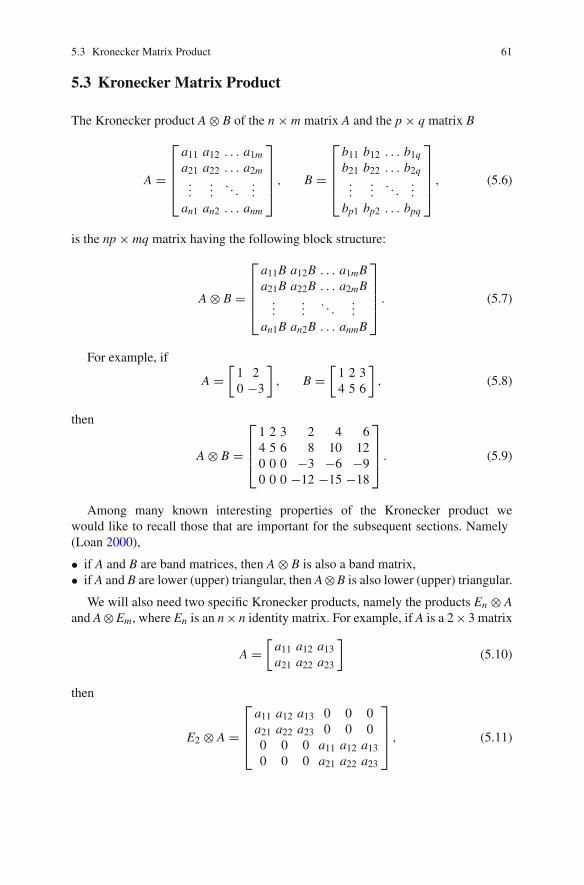
5.3 Kronecker Matrix Product 61
5.3 Kronecker Matrix Product
The Kronecker product A ⊗ B of the n × m matrix A and the p × q matrix B
A =
⎡⎢⎢⎢⎣
a11 a12 . . . a1m
a21 a22 . . . a2m...
.... . .
...
an1 an2 . . . anm
⎤⎥⎥⎥⎦ , B =
⎡⎢⎢⎢⎣
b11 b12 . . . b1q
b21 b22 . . . b2q...
.... . .
...
bp1 bp2 . . . bpq
⎤⎥⎥⎥⎦ , (5.6)
is the np × mq matrix having the following block structure:
A ⊗ B =
⎡⎢⎢⎢⎣
a11B a12B . . . a1mBa21B a22B . . . a2mB
......
. . ....
an1B an2B . . . anmB
⎤⎥⎥⎥⎦ . (5.7)
For example, if
A =[
1 20 −3
], B =
[1 2 34 5 6
], (5.8)
then
A ⊗ B =
⎡⎢⎢⎣
1 2 3 2 4 64 5 6 8 10 120 0 0 −3 −6 −90 0 0 −12 −15 −18
⎤⎥⎥⎦ . (5.9)
Among many known interesting properties of the Kronecker product wewould like to recall those that are important for the subsequent sections. Namely(Loan 2000),
• if A and B are band matrices, then A ⊗ B is also a band matrix,• if A and B are lower (upper) triangular, then A⊗B is also lower (upper) triangular.
We will also need two specific Kronecker products, namely the products En ⊗ Aand A ⊗ Em, where En is an n × n identity matrix. For example, if A is a 2 × 3 matrix
A =[
a11 a12 a13a21 a22 a23
](5.10)
then
E2 ⊗ A =
⎡⎢⎢⎣
a11 a12 a13 0 0 0a21 a22 a23 0 0 00 0 0 a11 a12 a130 0 0 a21 a22 a23
⎤⎥⎥⎦ , (5.11)
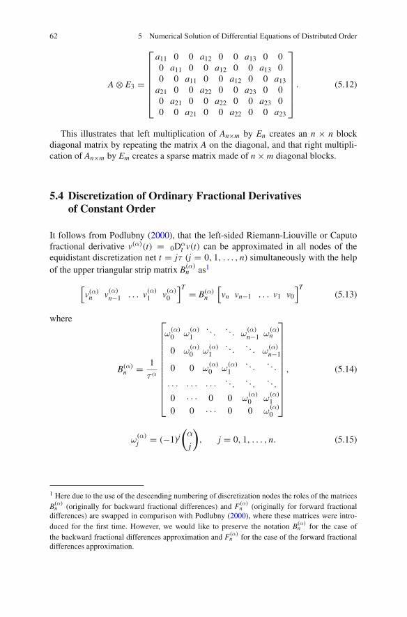
62 5 Numerical Solution of Differential Equations of Distributed Order
A ⊗ E3 =
⎡⎢⎢⎢⎢⎢⎢⎣
a11 0 0 a12 0 0 a13 0 00 a11 0 0 a12 0 0 a13 00 0 a11 0 0 a12 0 0 a13
a21 0 0 a22 0 0 a23 0 00 a21 0 0 a22 0 0 a23 00 0 a21 0 0 a22 0 0 a23
⎤⎥⎥⎥⎥⎥⎥⎦
. (5.12)
This illustrates that left multiplication of An×m by En creates an n × n blockdiagonal matrix by repeating the matrix A on the diagonal, and that right multipli-cation of An×m by Em creates a sparse matrix made of n × m diagonal blocks.
5.4 Discretization of Ordinary Fractional Derivativesof Constant Order
It follows from Podlubny (2000), that the left-sided Riemann-Liouville or Caputofractional derivative v(α)(t) = 0Dα
t v(t) can be approximated in all nodes of theequidistant discretization net t = jτ (j = 0, 1, . . . , n) simultaneously with the helpof the upper triangular strip matrix B(α)
n as1
[v(α)
n v(α)n−1 . . . v(α)
1 v(α)0
]T = B(α)n
[vn vn−1 . . . v1 v0
]T(5.13)
where
B(α)n = 1
τα
⎡⎢⎢⎢⎢⎢⎢⎢⎢⎢⎢⎢⎣
ω(α)0 ω
(α)1
. . .. . . ω
(α)n−1 ω
(α)n
0 ω(α)0 ω
(α)1
. . .. . . ω
(α)n−1
0 0 ω(α)0 ω
(α)1
. . .. . .
· · · · · · · · · . . .. . .
. . .
0 · · · 0 0 ω(α)0 ω
(α)1
0 0 · · · 0 0 ω(α)0
⎤⎥⎥⎥⎥⎥⎥⎥⎥⎥⎥⎥⎦
, (5.14)
ω(α)j = (−1)j
(α
j
), j = 0, 1, . . . , n. (5.15)
1 Here due to the use of the descending numbering of discretization nodes the roles of the matricesB(α)
n (originally for backward fractional differences) and F(α)n (originally for forward fractional
differences) are swapped in comparison with Podlubny (2000), where these matrices were intro-duced for the first time. However, we would like to preserve the notation B(α)
n for the case ofthe backward fractional differences approximation and F(α)
n for the case of the forward fractionaldifferences approximation.
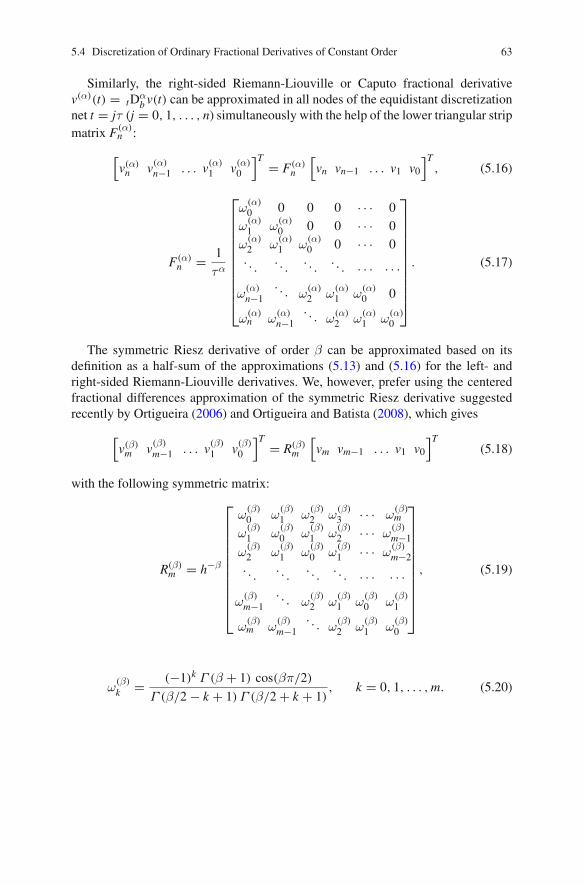
5.4 Discretization of Ordinary Fractional Derivatives of Constant Order 63
Similarly, the right-sided Riemann-Liouville or Caputo fractional derivativev(α)(t) = tDα
b v(t) can be approximated in all nodes of the equidistant discretizationnet t = jτ (j = 0, 1, . . . , n) simultaneously with the help of the lower triangular stripmatrix F(α)
n :
[v(α)
n v(α)n−1 . . . v(α)
1 v(α)0
]T = F(α)n
[vn vn−1 . . . v1 v0
]T, (5.16)
F(α)n = 1
τα
⎡⎢⎢⎢⎢⎢⎢⎢⎢⎢⎢⎣
ω(α)0 0 0 0 · · · 0
ω(α)1 ω
(α)0 0 0 · · · 0
ω(α)2 ω
(α)1 ω
(α)0 0 · · · 0
. . .. . .
. . .. . . · · · · · ·
ω(α)n−1
. . . ω(α)2 ω
(α)1 ω
(α)0 0
ω(α)n ω
(α)n−1
. . . ω(α)2 ω
(α)1 ω
(α)0
⎤⎥⎥⎥⎥⎥⎥⎥⎥⎥⎥⎦
. (5.17)
The symmetric Riesz derivative of order β can be approximated based on itsdefinition as a half-sum of the approximations (5.13) and (5.16) for the left- andright-sided Riemann-Liouville derivatives. We, however, prefer using the centeredfractional differences approximation of the symmetric Riesz derivative suggestedrecently by Ortigueira (2006) and Ortigueira and Batista (2008), which gives
[v(β)
m v(β)m−1 . . . v(β)
1 v(β)0
]T = R(β)m
[vm vm−1 . . . v1 v0
]T(5.18)
with the following symmetric matrix:
R(β)m = h−β
⎡⎢⎢⎢⎢⎢⎢⎢⎢⎢⎢⎣
ω(β)0 ω
(β)1 ω
(β)2 ω
(β)3 · · · ω
(β)m
ω(β)1 ω
(β)0 ω
(β)1 ω
(β)2 · · · ω
(β)m−1
ω(β)2 ω
(β)1 ω
(β)0 ω
(β)1 · · · ω
(β)m−2
. . .. . .
. . .. . . · · · · · ·
ω(β)m−1
. . . ω(β)2 ω
(β)1 ω
(β)0 ω
(β)1
ω(β)m ω
(β)m−1
. . . ω(β)2 ω
(β)1 ω
(β)0
⎤⎥⎥⎥⎥⎥⎥⎥⎥⎥⎥⎦
, (5.19)
ω(β)
k = (−1)k Γ (β + 1) cos(βπ/2)
Γ (β/2 − k + 1) Γ (β/2 + k + 1), k = 0, 1, . . . , m. (5.20)

64 5 Numerical Solution of Differential Equations of Distributed Order
5.5 Discretization of Ordinary Derivatives of Distributed Order
Using the matrix approach, the discretization of a derivative of distributed orderis very easy. Let us discretize the interval [a, b], in which the order α is changing,using the grid with the steps Δαk , not necessarily equidistant. Then we have
0Dw(α)t f (t) =
γ2∫γ1
w(α) 0Dαt f (t) dα ≈
p∑k=1
w(αk)(
0Dαkt f (t)
)Δαk (5.21)
≈p∑
k=1
w(αk)(
Bαkn fn
)Δαk =
( p∑k=1
Bαkn w(αk)Δαk
)fn. (5.22)
In other words, the discrete analog of distributed-order differentiation is given bythe matrix that we will further denote as Bw(α)
n,p ,
Bw(α)n,p =
p∑k=1
Bαkn w(αk)Δαk, (5.23)
and we can obtain the values of the distributed-order derivative at all pointstj (j = 1, . . . , n) at once using the following relationship:
0Dw(α)t f (t) ≈ Bw(α)
n,p fn. (5.24)
In the notation Bw(α)n,p the order w(α) means the function describing the distrib-
ution of orders α in the interval [γ1, γ2], and the second index p is the number ofdiscretization steps for α; the first index n, as above, is the number of discretizationsteps with respect to the variable t.
The visualization of the formula (5.21) is shown in Fig. 5.1. On each k-th layerof the shown “cake” the input vector fn of the values of the function f (t) at thenodes tj is multiplied by the matrix Bαk
n and gives the output vector of the valuesof the fractional derivative 0Dαk
t at the same nodes tj. Those vectors 0Dαkt are then
multiplied by weights w(αk) and discretization steps Δαk , and the final summationwith respect to k (“summation across the layers of orders”) gives the vector of thedistributed-order derivative 0Dw(α)
t evaluated at the nodes tj (j = 1, . . . , n).
5.6 Discretization of Partial Derivatives of Distributed Order
In contrast with generally used numerical methods, where the solution is obtainedstep-by-step by moving from the previous time layer to the next one, let us considerthe whole time interval of interest at once. This allows us to create a net of

5.6 Discretization of Partial Derivatives of Distributed Order 65
Fig. 5.1 Visualization of numerical evaluation of distributed-order derivatives with the help of thematrix approach
discretization nodes. In the simplest case of one spatial dimension this step givesa 2D net of nodes. An example of such discretization is shown in Fig. 5.2. The valuesof the unknown function in inner nodes (shaded area in Fig. 5.2) are to be found. Thevalues at the boundaries are known, they are used later in constructing the system ofalgebraic equations.
The system of algebraic equations is obtained by approximating the equation inall inner nodes simultaneously (this gives the left-hand side of the resulting systemof algebraic equations) and then utilizing the initial and boundary conditions (thevalues of which appears in the right-hand side of the resulting system).
The discretization nodes in Fig. 5.2 are numbered from right to left in each timelevel, and the time levels are numbered from bottom to top. We use such numberingfor the clarity of presentation of our approach, although standard numberings workequally well.
The simplest implicit discretization scheme used for numerical solution of partialdifferential equations, like diffusion equation, is shown in Fig. 5.3, where the twonodes in time direction are used for approximating the time derivative, and the threepoints in spatial direction are used for the symmetric approximation of the spatialderivative. The stencil in Fig. 5.3 involves therefore only two time layers. If weconsider fractional-order time derivative or distributed-order derivative, then we haveto involve all time levels starting from the very beginning. This is shown in Fig. 5.4for the case of five time layers.
Similarly, if in addition to time derivative of distributed order or of fractional orderwe also consider symmetric spatial derivatives of distributed order or fractional order,then we have to use all nodes at the considered time layer. This most general situationis shown in Fig. 5.5.
Let us consider the nodes (ih, jτ ), j = 0, 1, 2, . . . , n, corresponding to alltime layers at i-th spatial discretization node. Similarly to the case of constantfractional orders (Podlubny 2000), all values of α-th order time derivative of u(x, t)at these nodes are approximated using the discrete analogue of distributed-orderdifferentiation:

66 5 Numerical Solution of Differential Equations of Distributed Order
Fig. 5.2 Nodes and theirright-to-left, and bottom-to-top numbering
[u(w(α))
i,n u(w(α))i,n−1 . . . u(w(α))
i,2 u(w(α))i,1 u(w(α))
i,0
]
= Bw(α)n,p
[ui,n ui,n−1 . . . ui,2 ui,1 ui,0
]T. (5.25)
In order to obtain a simultaneous approximation of α-th order time derivative ofu(x, t) in all nodes shown in Fig. 5.2, we need to arrange all function values uij atthe discretization nodes to the form of a column vector:
Unm =[um,n um−1,n . . . u1,n u0,n
um,n−1 um−1,n−1 . . . u1,n−1 u0,n−1
. . . . . . . . .
um,1 um−1,1 . . . u1,1 u0,1
um,0 um−1,0 . . . u1,0 u0,0
]T. (5.26)
In visual terms of Fig. 5.2, we first take the nodes of n-th time layer, then thenodes of (n − 1)-th time layer, and so forth, and put them in this order in a verticalcolumn stack.
The matrix that transforms the vector Unm to the vector Uw(α)t of the partial
derivative of distributed order w(α) with respect to time variable can be obtained asa Kronecker product of the matrix Bw(α)
n,p , which corresponds to the ordinary derivativeof distributed order w(α) (recall that n is the number of time steps), and the unit matrixEm (recall that m is the number of spatial discretization steps):
Tw(α)mn = Bw(α)
n,p ⊗ Em. (5.27)

5.6 Discretization of Partial Derivatives of Distributed Order 67
This is illustrated in Fig. 5.6, where the nodes denoted as white and grey are usedto approximate the fractional-order time derivative at the node shown in grey.
Similarly, the matrix that transforms the vector U to the vector Uϕ(β)x of the
derivative of distributed order ϕ(β) with respect to spatial variable can be obtainedas a Kronecker product of the unit matrix En (recall that n is the number of spatialdiscretization nodes), and the matrix Rϕ(β)
m,p , which corresponds to symmetric Rieszordinary derivative of distributed order ϕ(β) (recall that m is the number of timesteps):
Sϕ(β)mn = En ⊗ Rϕ(β)
n,p . (5.28)
This is also illustrated in Fig. 5.6, where the nodes denoted as black and greyare used to approximate the symmetric fractional-order Riesz derivative at the samenode shown in grey.
Having these approximations for partial fractional derivatives with respect to bothvariables, we can immediately discretize, for example, the diffusion equation in termsof time- and space-derivatives of distributed order by simply replacing the derivativeswith their discrete analogs (Fig. 5.7). Namely, the equation
0Dw(α)t u − χ
∂ϕ(β)u
∂|x|ϕ(β)= f (x, t) (5.29)
is discretized as {Bw(α)
n,p ⊗ Em − χ En ⊗ Rϕ(β)m,p
}unm = fnm. (5.30)
5.7 Initial and Boundary Conditions for Using the MatrixApproach
It is always emphasized in case of the matrix approach to solution of differentialequations that initial and boundary conditions must be equal to zero. If it is not so,then an auxiliary unknown function must be introduced, which satisfies the zero initialand boundary conditions. In this way, the non-zero initial and boundary conditionsmoves to the right-hand side of the equation for the new unknown function. Afterobtaining the solution for the auxiliary function, the backward substitution gives thesolution of the original equation.
5.8 Implementation in MATLAB
A set of MATLAB routines implementing the described method is provided fordownload (Podlubny 2011). Those routines require the previously published toolbox

68 5 Numerical Solution of Differential Equations of Distributed Order
Fig. 5.3 A stencil for integer-order derivatives
Fig. 5.4 A stencil in caseof distributed-order andfractional time derivative andsecond-order spatial deriv-ative
Fig. 5.5 A stencil in caseof distributed-order andfractional-order time andspatial derivatives
Fig. 5.6 Discretization ofpartial derivaives
for numerical solution of differential equations of arbitrary (fractional) constant order(Podlubny et al. 2008).
The function DOBAN returns the matrix for the backward difference approxi-mation of the left-sided distributed-order derivative, the function DOFAN returns thematrix for approximating the right-sided distributed-order derivative, DORANORTreturn the matrix for approximating the symmetric Riesz distributed-order derivative.
The use of these routines is illustrated by the demo functions included in thetoolbox.
5.9 Numerical Examples
The use of the matrix approach for numerical solution of differential equations withderivatives of distributed orders is illustrated below on three examples that generalizethe standard frequently used models of the applied fractional calculus. The relaxation,oscillation, and diffusion equations play extremely important role in numerous fields

5.9 Numerical Examples 69
Fig. 5.7 Discretization ofpartial derivaives and of theequation
of science and engineering, and, because of their importance, they are also often usedfor benchmarking new methods and algorithms.
To the knowledge of the authors, these are the first examples of numerical solutionof such distributed-order problems.
It is worth mentioning that existence and uniqueness of solutions of such typesof distributed-order differential equations in the particular case of w(α) = 1 wereinvestigated by Pskhu (2005).
5.9.1 Example 1: Distributed-Order Relaxation
Let us consider the following initial value problem for the distributed-order relaxationequation:
0Dw(α)t x(t) + bx(t) = f (t), (5.31)
x(0) = 1, (5.32)
where the distribution of the orders α is given by the function w(α) = 6 α (1 − α),(0 ≤ α ≤ 1). To be able to use the matrix approach, we need zero initial condition.Introducing an auxiliary function u(t),
x(t) = u(t) + 1
gives the following initial value problem for the new unknown u(t):
0Dw(α)t u(t) + bu(t) = f (t) − b, (5.33)
u(t) = 0. (5.34)
The discretization of equation (5.33) gives the following system of algebraicequations in the matrix form:
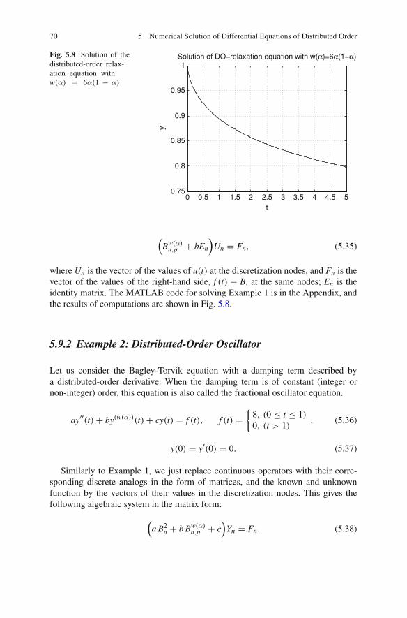
70 5 Numerical Solution of Differential Equations of Distributed Order
Fig. 5.8 Solution of thedistributed-order relax-ation equation withw(α) = 6α(1 − α)
0 0.5 1 1.5 2 2.5 3 3.5 4 4.5 50.75
0.8
0.85
0.9
0.95
1Solution of DO−relaxation equation with w(α)=6α(1−α)
t
y
(Bw(α)
n,p + bEn
)Un = Fn, (5.35)
where Un is the vector of the values of u(t) at the discretization nodes, and Fn is thevector of the values of the right-hand side, f (t) − B, at the same nodes; En is theidentity matrix. The MATLAB code for solving Example 1 is in the Appendix, andthe results of computations are shown in Fig. 5.8.
5.9.2 Example 2: Distributed-Order Oscillator
Let us consider the Bagley-Torvik equation with a damping term described bya distributed-order derivative. When the damping term is of constant (integer ornon-integer) order, this equation is also called the fractional oscillator equation.
ay′′(t) + by(w(α))(t) + cy(t) = f (t), f (t) ={
8, (0 ≤ t ≤ 1)
0, (t > 1), (5.36)
y(0) = y′(0) = 0. (5.37)
Similarly to Example 1, we just replace continuous operators with their corre-sponding discrete analogs in the form of matrices, and the known and unknownfunction by the vectors of their values in the discretization nodes. This gives thefollowing algebraic system in the matrix form:
(a B2
n + b Bw(α)n,p + c
)Yn = Fn. (5.38)

5.9 Numerical Examples 71
Fig. 5.9 Solution of thedistributed-order oscil-lator equation (Bagley-Torvik equation) withw(α) = 6α(1 − α)
0 5 10 15 20 25 30−2
−1
0
1
2
3
4Solution of Bagley−Torvik DO−equation with w(α)=6α(1−α)
The MATLAB code for solving Example 2 is in the Appendix, and the results ofcomputations are shown in Fig. 5.9.
5.9.3 Example 3: Distributed-Order Diffusion
The last example that is provided in this section is an initial value problem for apartial differential equation with a derivative of distributed-order w(α) with respectto time variable t and with a constant-order symmetric fractional derivative of orderβ with respect to the spatial variable x:
0Dw(α)t y − ∂βy
∂|x|β = f (x, t) (5.39)
y(0, t) = 0, y(1, t) = 0; y(x, 0) = 0. (5.40)
In order to be able to check for a “backward compatibility” of the obtained solutionwith the solution of the classical diffusion equation and with the solution of theconstant-order fractional diffusion equation, we take f (x, t) = 8.
Again, we just replace continuous operators with their corresponding discreteanalogs in the form of matrices, and the known and unknown function by the vectorsof their values in the discretization nodes. This gives the following algebraic systemin the matrix form:
(Bw(α)
n,p ⊗ Em − En ⊗ Rβm
)Ynm = Fnm. (5.41)

72 5 Numerical Solution of Differential Equations of Distributed Order
00.01
0.020.03
0.040.05
0.06
00.2
0.40.6
0.810
0.2
0.4
0.6
0.8
1
t
=2*(1−alf), = 2
x
y(x,
t)
Fig. 5.10 Solution of distributed-order diffusion equation with w1(α) = 2(1 − α)
Here we demonstrate that distributed-order derivatives, integer-order derivativesand fractional-order derivatives can appear in the same equations and are treated inthe same manner for the purpose of numerical solution using the matrix approach.
The MATLAB code for solving Example 3 is also provided in the Appendix. Theresults of computations are shown in Fig. 5.10 for the case w1(α) = 2(1 − α), andin Fig. 5.11 for the case w2(α) = 2α. Although we have
1∫0
w1(α) dα =1∫
0
w2(α) dα = 1,
the obtained solutions are different because of different weights assigned by thefunctions w1(α) and w2(α) to the fractional derivatives of orders close to 0 and 1.
5.10 Chapter Summary
In this chapter we introduced the extension of Podlubny’s matrix approach to thecase of distributed-order derivatives. The matrix approach provides an extremelyconvenient language and framework for discretization of differentiation of anyorder—integer, fractional, and distributed order. Using discrete analogs of all thoseforms of differentiation, one can easily discretize differential equations with all

5.10 Chapter Summary 73
0.020.4
tx
0
0.2
0.4
0.6
0.8
1
0 00.2
0.60.8
1
0.010.030.040.05
0.06
y(x,
t)
φ = 2*alf, β = 2
Fig. 5.11 Solution of distributed-order diffusion equation with w2(α) = 2α
possible combinations of derivatives—classical integer-order derivatives, left- andright-sided fractional order derivatives, symmetric fractional derivatives, and left-sided, right-sided, and symmetric distributed-order derivatives.
We have provided examples of solution of the three important types of problemsthat are important for applications and appear in many fields of science andengineering. The MATLAB code provided in the Appendix demonstrates how easyit is using the matrix approach.
References
Bulgakov BV (1954) Kolebaniya (Vibrations). Gostekhizdat, MoscowGantmakher FR (1988) Theory of matrices. Nauka, MoscowLoan CFV (2000) The ubiquitous Kronecker product. J Comput Appl Math 123:85–100Ortigueira MD (2006) Riesz potential operators and inverses via fractional centred derivatives. Int
J Math Math Sci 48391:1–12Ortigueira MD, Batista AG (2008) On the relation between the fractional Brownian motion and the
fractional derivatives. Phys Lett A 372:958–968Podlubny I (2000) Matrix approach to discrete fractional calculus. Fract Cal Appl Anal
3(4):359–386Podlubny I (2011) Matrix approach to distributed-order ODEs and PDEs. http://www.mathworks.
com/matlabcentral/fileexchange/Podlubny I, Skovranek T, Vinagre BM (2008) Matrix approach to discretization of ODEs and PDEs
of arbitrary real order. http://www.mathworks.com/matlabcentral/fileexchange/22071Podlubny I, Skovranek T, Vinagre BM (2009a) Matrix approach to discretization of ordinary and
partial differential equations of arbitrary real order: the matlab toolbox. In: Proceedings of theASME 2009 international design engineering technical conferences and Computers and infor-mation in engineering conference IDETC/CIE 2009 August 30–September 2, 2009, San Diego,USA, article DETC2009-86944

74 5 Numerical Solution of Differential Equations of Distributed Order
Podlubny I, Chechkin A, Skovranek T, Chen YQ, Vinarge BM (2009b) Matrix approach to discretefractional calculus ii: partial fractional differential equations. J Comput Phys 228(8):3137–3153
Podlubny I, Skovranek T, Verbickij V, Vinagre BM, Chen YQ, Petras I (2011) Discrete fractionalcalculus: non-equidistant grids and variable step length. In: Proceedings of the ASME 2011international design engineering technical conferences and computers and information inengineering conference IDETC/CIE 2011 August 28–31, 2011, Washington, DC, USA, articleDETC2011-47623
Pskhu AV (2005) Differencial’nye uravneniya drobnogo poryadka (Partial differential equations offractional order). Nauka, Moscow (in Russian)
Skovranek T, Verbickij V, Tarte Y, Podlubny I (2010) Discretization of fractional-order operatorsand fractional differential equations on a non-equidistant mesh. In: Proceedings of the 4TH IFACworkshop on fractional differentiation and its applications, Badajoz, Spain, October 18–20, 2010,article FDA10-157
Suprunenko DA, Tyshkevich RI (1966) Commutative matrices. Nauka i Tekhnika, Minsk

Chapter 6Future Topics
In previous chapters, methods and tools for the modeling of distributed-ordersystems were discussed, which include stability analysis of distributed-order sys-tems in four cases of the weighting function of order, and two special cases: doublenoncommensurate orders and N -term noncommensurate orders. Distributed-ordersignal processing technique and optimal distributed-order damping strategies werestudied. A general approach to numerical solution to discretization of distributed-order derivatives and integrals, and to numerical solution of ordinary and partialdifferential equations of distributed order was proposed.
Let us now outline possible topics for future research in the field of distributed-order systems.
6.1 Geometric Interpretation of Distributed-OrderDifferentiation as a Framework for Modeling
Distributed-order derivatives can be considered as a kind of averaging operators.However, they do not average the values of parameters over a set of values—theyaverage the behavior of individual objects or processes over a set of objects orprocesses of the same type.
Let us consider an understandable example of the impact of advertising on thecrowd consisting of a large number of individuals. The broadcast of an advertisementis a unit-step input; this can be interpreted as charging the memory of individuals tosome initial value.
The impact of such input on an individual vanishes in time due to propertiesof human’s memory (memory relaxation, or forgetting). Suppose it is possible toclassify individuals with respect to the properties of their memory into p groups.The process of memory relaxaation in the i-th group of individuals can be describedby an initial-value problem for a two-term fractional differential equation in termsof Caputo derivatives with non-zero initial condition:
Z. Jiao et al., Distributed-Order Dynamic Systems, SpringerBriefs in Control, 75Automation and Robotics, DOI: 10.1007/978-1-4471-2852-6_6,© The Author(s) 2012

76 6 Future Topics
0Dαit x(t) + bx(t) = 0, x(0) = 1, (6.1)
where the order αi is from the interval [0, 1]; we assume that α1 < α2 < . . . < αp.Denoting wi the number of individuals in i-th group normalized with respect to
the total number of individuals (so that∑
wi = 1), we obtain a piecewise-constantweighting function
w(α) = wi for αi < α ≤ αi+1 (i = 1, . . . , p − 1). (6.2)
Then the averaged behavior of the crowd can be described as
p−1∑i=1
w(αi ) 0Dαit x(t)�αi = 0Dw(α)
t x(t), (6.3)
which is a distributed-order derivative, and the equation describing the process of thememory relaxation of a crowd takes on the form of a distributed-order differentialequation
0Dw(α)t x(t) + bx(t) = 0, (6.4)
x(0) = 1. (6.5)
Of course, in many situations the function w(α) describing the distribution oforders α can be modeled as a continuous function.
The outlined general framework for creation of distributed order models can beused for modeling multiscale and multifractal processes, multiagent systems, and inmany other cases where the subject of study consists of “individuals”.
The above considerations are presented in graphical form in Fig. 6.1, which givesa geometric interpretation of distributed-order differentiation and integration.
6.2 From Positive Linear Time-Invariant Systemsto Generalized Distributed-Order Systems
Let us consider a linear differential equation with fractional-order derivatives,
n∑k=1
ak 0Dαkt x(t) = f (t), (6.6)
where all coefficients are positive constants: ak > 0, k = 1, . . . , n. Without the lossof generality, we can assume that

6.2 From Positive Linear Time-Invariant Systems 77
Fig. 6.1 Geometric interpretation of distributed-order differentiation as a framework for creatingdistributed-order models
n∑k=1
ak = 1.
Introducing the weighting function
w(α) =n∑
k=1
akδ(α − αk), (6.7)
we can write the Eq. (6.6) in the form of a distributed-order differential equation:
0Dw(α)t x(t) = f (t). (6.8)
This means that properties of positive linear time-invariant systems shouldfollow from the properties of distributed-order systems with a positive function w(α)
describing the distribution of orders.Such a change of the viewpoint means also that the problem of identification of
parameters of linear time invariant systems like (6.6) can be replaced by a moregeneral and more interesting problem of identification of a most appropriate shapeof the function w(α) of a system described by Eq. (6.7).
Similarly, the theory of stability of linear time-invariant systems can be overcomeby the theory of stability of distributed-order systems.
Even more possibilities open if the distributed-order derivative is written in theform

78 6 Future Topics
0Dw(α)
t x(t) =γ2∫
γ1
0Dαt x(t)dW (α). (6.9)
If the function W (α) is differentiable and W ′(α) = w(α), then we have thedistributed-order derivative considered in this book; otherwise there is large spacefor further generalizations with potential applications to self-similar, fractal andmultifractal systems.
6.3 From PID Controllers to Distributed-OrderPID Controllers
PID Controller
The classical PID controller, which is the most commonly used feedback controllerin industry, can be considered as a particular form of lead-lag compensation in thefrequency domain. Its transfer function can be expressed as C1(s) = K p + Ki
s +Kds. The PID controller algorithm involves three separate constant parameters: theproportional P , the integral I and derivative D. These values can be interpreted interms of time: P depends on the present error, I on the accumulation of past errors,and D is a prediction of future errors, based on current rate of change.
Fractional-Order PIλDμ Controller
Podlubny (1999) proposed a generalization of the PID controller, namely the PIλDμ
controller. Its transfer function can be expressed as C2(s) = K p + Kisλ + Kdsμ, which
involves an integrator of order λ and a differentiator of order λ. Better response of thistype of controller in comparison with the classical PID controller was demonstratedin that work. For results about using PIλDμ controller to some real world systems,please refer to Li et al. (2009) and Luo and Chen (2009) etc.
Distributed-Order PIλ(α)Dμ(α) Controller
As a generalization of PIλDμ controller, distributed-order PID controller of thefollowing form
C3(s) = K p +∫ 1
−1w(α)sαdα

6.3 From PID Controllers to Distributed-Order PID Controllers 79
where w(α) =N∑
i=0wiα
i ≈ w0 + w1α
or
C3(s) = K p + Ki
∫ γ1
0
1
sαdα + Kd
∫ γ2
0sαdα
will be our future work.
References
Li HS, Luo Y, Chen YQ (2009) A fractional order proportional and derivative (FOPD) motioncontroller: tuning rule and experiments. IEEE Trans Control Syst Technol 18(2):1–5
Luo Y, Chen YQ (2009) Fractional order [proportional derivative] controller for a class of fractionalorder systems. Automatica 45(10):2446–2450
Podlubny I (1999) Fractional-order systems and PIλDμ controllers. IEEE Trans Autom Control44(1):208–214

Appendix AMATLAB Codes
A.1 Stable Boundary of Distributed-Order LinearTime-Invariant Systems
% The following matlab code describes how to plot the stable% boundary of distributed-order linear time-invariant% system
xð1Þ ¼ 0; % set the initial value of x
yð1Þ ¼ 0; % set the initial value of y
% the computed number of the stable boundaryw ¼ logspaceð�200;2;10000Þ;
% the stable boundary of distributed-order% system of case 1: W (\alpha) = 1for i ¼ 1 : length ðwÞ
xðiÞ ¼ ð2�pi�wðiÞ � 4�logðwðiÞÞÞ=ð4�ðlogðwðiÞÞÞ^2þ pi^2Þ;yðiÞ ¼ ð4�wðiÞ�logðwðiÞÞ þ 2�piÞ=ð4�ðlogðwðiÞÞÞ^2þ pi^2Þ;
end
% the stable boundary of distributed-order% system of case 2: w(\alpha) = \alphafor i ¼ 1 : lengthðwÞ
xðiÞ ¼ ðð�1� logðwðiÞÞÞ�ððlogðwðiÞÞÞ^2� pi^2=4Þ þ . . .
pi�logðwðiÞÞ�ðwðiÞ � pi=2ÞÞ=ððlogðwðiÞÞÞ^2þ pi^2=4Þ^2;yðiÞ ¼ ððwðiÞ � pi=2Þ�ððlogðwðiÞÞÞ^2� pi^2=4Þ þ . . .
pi�logðwðiÞÞ�ð1þ logðwðiÞÞÞÞ=ððlogðwðiÞÞÞ^2þ pi^2=4Þ^2;end
% the stable boundary of distributed-order% system of case 3: w(\alpha) = \delta(\alpha - \beta)beta ¼ 0:5;
Z. Jiao et al., Distributed-Order Dynamic Systems, SpringerBriefs in Control,Automation and Robotics, DOI: 10.1007/978-1-4471-2852-6,� The Author(s) 2012
81

for i ¼ 1 : lengthðwÞxðiÞ ¼ wðiÞ^beta�cosðpi�beta=2Þ;yðiÞ ¼ wðiÞ^beta�sinðpi�beta=2Þ;
end
% the stable boundary of fractional-order% system with double noncommensurate ordersbeta1 ¼ sqrt ð2Þ � 1;beta2 ¼ sqrt ð3Þ � 1;for i ¼ 1 : lengthðwÞ
xðiÞ ¼ wðiÞ^beta1�cosðpi�beta1=2Þ þ wðiÞ^beta2�cosðpi�beta2=2Þ;yðiÞ ¼ wðiÞ^beta1�sinðpi�beta1=2Þ þ wðiÞ^beta2�sinðpi�beta2=2Þ;
end
% plot the stable boundaryplot(x,y)hold onplot(x,-y)axis squaregrid onxlabel(’Real axis’);ylabel(’Imag axis’);
A.2 Bode Plots of Distributed-Order LinearTime-Invariant Systems
% The following matlab code describes how to plot the Bode% plots of distributed-order linear time-invariant system
function ½bd� ¼ bode dosðTsÞ
% Ts: The sampling periodif Ts\ ¼ 0;sprintf(’%s’,’Sampling period has to be positive’),return,end
% rad./sec. Nyquist frequencywmax0 ¼ 2�pi=Ts=2;
wmax ¼ floorðlog10ðwmax0ÞÞ þ 1;wmin ¼ wmax� 5;w ¼ logspaceðwmin;wmax;1000Þ;j ¼ sqrtð�1Þ;
% the Bode plot of distributed-order% system of case 1: w(\alpha)=1srfr ¼ logðj:�wÞ:=ðj:�w� 1þ logðj:�wÞÞ;
82 Appendix A: MATLAB Codes

% the Bode plot of distributed-order% system of case 2: w(alpha)=\alphasrfr ¼ ðlogðj:�wÞÞ:^2:=ðj:�w� 1� logðj:�wÞ þ logðj:�wÞ:�logðj:�wÞÞ;
% the Bode plot of distributed-order% system of case 3: w(\alpha)=\delta(\alpha-\beta)srfr ¼ 1:=ððj:�wÞ:^0:5þ 1Þ;
% the Bode plot of fractional-order% system with double noncommensurate orders%srfr ¼ 1:=ððj:�wÞ:^ðsqrtð3Þ � 1Þ þ ðj:�wÞ: ^0:5þ ðj:�wÞ:^ðsqrtð2Þ � 1Þ þ 1Þ;
% plot the magnitude propertysubplot(2,1,1);semilogxðw;20�log10ðabsðsrfrÞÞÞ;hold on;ylabel(’Magnitude (dB)’);grid on;
% plot the phase propertysubplot(2,1,2);semilogxðw; ð180=piÞ�ðangleðsrfrÞÞÞ;xlabel(’Frequency (Hz)’);ylabel(’Phase (degrees)’);
end
A.3 Impulse Responses of Distributed-Order LinearTime-Invariant Systems
% The following matlab code describes how to plot the impulse responses% of distributed-order linear time-invariant system based on NILT% technique% Code adapted from
% L. Bran.cL.k. Programs for fast numerical inversion of Laplace% transforms in MATLAB language environment. In Proceedings of the% 7th Conference MATLABf99, pages 27.39, Prague, Nov. 1999. Czech% Republic.
function ½id� ¼ BICO iridðTsÞ;
% Ts: The sampling period% the impulse response of distributed-order% system of cases 1: w(\alpha)=1F ¼ C�logðsÞ:�ððs� 1Þ�eyeð2Þ � A�logðsÞÞ:^ð�1Þ�B;
% the impulse response of distributed-order% system of cases 2: w(\alpha) = \alphaF ¼ C�logðsÞ:2:�ððs� 1� logðsÞÞ�eyeð2Þ � A�logðsÞ:^2Þ:^ð�1Þ�B;
Appendix A: MATLAB Codes 83

% the impulse response of distributed-order% system of case 3: w(\alpha)=\delta(\alpha-\beta)F ¼ C�ðs:^beta�eyeð2Þ � AÞ:^ð�1Þ�B;
% the Bode plot of fractional-order% system with double noncommensurate ordersF ¼ C�ððs:^beta1þ s:^;beta2Þ�eyeð2Þ � AÞ:^ð�1Þ�B;
alfa ¼ 0;M ¼ 3072;P ¼ 20;Er ¼ 1e� 10;tm ¼ M�Ts;wmax0 ¼ 2�pi=Ts=2;L ¼ M;Taxis ¼ ½0 : L� 1��Ts;n=1:L-1;n ¼ n�Ts;q1 ¼ q;N ¼ 2�M;qd ¼ 2�Pþ 1;t ¼ linspaceð0;tm;MÞ;NT ¼ 2�tm�N=ðN� 2Þ;omega ¼ 2�pi=NT;c ¼ alfa� logðErÞ=NT;s ¼ c� i�omega�ð0 : Nþ qd� 1Þ;Fsc ¼ fevalðF;sÞ;ft ¼ fftðFscð1 : NÞÞ;ft ¼ ftð1 : MÞ;q ¼ FscðNþ 2 : Nþ qdÞ:=FscðNþ 1 : Nþ qd� 1Þ;d ¼ zerosð1;qdÞ;e ¼ d;dð1Þ ¼ FscðNþ 1Þ;dð2Þ ¼ �qð1Þ;z ¼ expð�i�omega�tÞ;
for r ¼ 2 : 2 : qd� 1w ¼ qd� r;eð1 : wÞ ¼ qð2 : wþ 1Þ � qð1 : wÞ þ eð2 : wþ 1Þ;dðrþ 1Þ ¼ eð1Þ;if r[2
qð1 : w� 1Þ ¼ qð2 : wÞ:�eð2 : wÞ:=eð1 : w� 1Þ;dðrÞ ¼ �qð1Þ;end
endA2 ¼ zerosð1;MÞ;B2 ¼ onesð1;MÞ;A1 ¼ dð1Þ�B2;B1 ¼ B2;for n ¼ 2 : qdA ¼ A1þ dðnÞ�z:�A2;B ¼ B1þ dðnÞ�z:�B2;
84 Appendix A: MATLAB Codes

A2 ¼ A1;B2 ¼ B1;A1 ¼ A;B1 ¼ B;end
ht ¼ expðc�tÞ=NT:�ð2�realðftþ A:=BÞ � Fscð1ÞÞ;½b1;a1� ¼ stmcbðhtð1 : endÞ:�Ts;q1;q1;100Þ;
sprintf(’Impulse response of approximated transfer function:’)
sr ¼ tfðb1;a1;TsÞ;hhat ¼ impulseðsr;TaxisÞ;figureplot(t,ht,’b’);grid on;
xlabel(’time axis’);ylabel(’impulse response’);xlim([0,30])
A.4 Solution of Distributed-Order Relaxation Equation
% (1) Prepare constants and nodes% (this is the longest part of the script):h ¼ 0:01; % step of discretization in spacet ¼ 0:h:5; % step of discretization in timeN ¼ lengthðtÞ þ 1; % number of nodesB ¼ 0:1; % coefficient of the equationf ¼ 00þ 0�t0; % right-hand sideM ¼ zerosðN;NÞ; % pre-allocate matrix M for the system
% (2) Write the discretization matrix
M ¼ dobanð06�alf:�ð1� alfÞ0;½01�;0:01;N� 1;hÞ þ B�eyeðN� 1;N� 1Þ;
% (3) Compute the right-hand side at discretization nodes:
F ¼ eval ð½f0 � B0�;tÞ0;
% (4) Utilize zero initial condition:
M ¼ eliminatorðN� 1; ½1�Þ�M�eliminatorðN� 1; ½1�Þ0;F ¼ eliminatorðN� 1; ½1�Þ�F;
% (5) And solve the system MY ¼ F :Y = M\F;
% (6) Pre-pend the zero initial value% (that one due to zero initial condition)Y0 ¼ ½0;Y�;
Appendix A: MATLAB Codes 85

% Plot the solution:U ¼ Y0þ 1;plot(t, U, ’k’)
A.5 Solution of Distributed-Order Oscillation Equation
% (1) Prepare constants and nodes% (this is the longest part of the script):A ¼ 1;B ¼ 1;C ¼ 1; % coefficients of the Bagley-Torvik equationh ¼ 0:075; % step of discretizationT ¼ 0:h:30; % nodesN ¼ 30=hþ 1; % number of nodesM ¼ zerosðN;NÞ; % pre-allocate matrix M for the system
% (2) Make the matrix for the entire equation --- this is really easy:
M ¼ A�banð2;N;hÞ þ B�dobanð06�alf:�ð1� alfÞ0; ½01�;0:01;N;hÞ þ . . .C�eyeðN;NÞ;
% (3) Make right-hand side:
F ¼ 8�ðT\ ¼ 1Þ0;
% (4) Utilize zero initial conditions:
M ¼ eliminatorðN; ½12�Þ�M�eliminatorðN; ½12�Þ0;F ¼ eliminatorðN; ½12�Þ�F;
% (5) Solve the system MY ¼ F :Y = M\F;
% (6) Pre-pend the zero values (those due to zero initial conditions)Y0 ¼ ½0;0;Y�;
% Plot the solution:plot(T,Y0,’k’)grid on
A.6 Solution of Distributed-Order Diffusion Equation
alpha ¼0 2�alf0 ;beta ¼ 2; % First, define the orders:a2 ¼ 1; % coefficient from the diffusion equationL ¼ 1; % length of spatial interval
% Number of spatial steps ? 1 is:m ¼ 21;% 11, 21% Number of steps in time ? 1 is:n ¼ 148;% 37, 148h ¼ L=ðm� 1Þ;tau ¼ h^2=ð6�a2Þ; % space step, time step
86 Appendix A: MATLAB Codes

% generating the matrix for approximation% alpha-th order derivative with respect to time
B1 ¼ dobanðalpha; ½01�;0:01;n� 1;tauÞ0;TD ¼ kronðB1;eyeðmÞÞ; % time derivative matrixB2 ¼ ransymðbeta;m;hÞ; % beta-th order derivative with respect to XSD ¼ kronðeyeðn� 1Þ;B2Þ; % spatial derivative matrixSystemMatrix ¼ TD� a2�SD; % matrix corresponding to
discretization% in space and time
% remove columns with ’1’ and ’m’ from SystemMatrixS ¼ eliminator ðm; ½1m�Þ;SK ¼ kronðeyeðn� 1Þ;SÞ;SystemMatrix without columns 1 m ¼ SystemMatrix�SK0;
% remove rows with ’1’ and ’m’ from SystemMatrix_without_columns_1_m
S ¼ eliminatorðm; ½1m�Þ;SK ¼ kronðeyeðn� 1Þ;SÞ;SystemMatrix without rows columns 1 m ¼ . . .
SK�SystemMatrix without columns 1 m;% Right hand sideF ¼ 8�onesðsizeðSystemMatrix without rows columns 1 m;1Þ;1Þ;
% Solution of the systemY ¼ SystemMatrix without rows columns 1 mnF
% Reshape solution array -- values for k-th time step% are in the k-th column of YS:
YS ¼ reshapeðY;m� 2;n� 1Þ;YS ¼ fliplrðYSÞ;U ¼ YS;
% plot graph½rows;columns� ¼ sizeðUÞ;U ¼ ½zerosð1;columnsÞ;U;zerosð1;columnsÞ�;U ¼ ½zerosð1;mÞ0 U�;½XX;YY� ¼ meshgridðtau�ð0 : n� 1Þ;h�ð0 : m� 1ÞÞ;
mesh(XX,YY,U)xlabel(’t’); ylabel(’x’); zlabel(’y(x,t)’);title([’\phi =’, num2str(alpha), ’, \beta = ’, … num2str(beta)])set(gca, ’xlim’, [0 tau*n], ’zlim’, [0 1]); box on
Appendix A: MATLAB Codes 87

Index
BBounded-input bounded-output stability, 25
CCaputo’s fractional-order derivative
definition, 3Constant phase element, 4CRONE control, 5
DDifferentiator, 45Digital filter, 43Distributed-order damping, 48Distributed-order differential equation, 6Distributed-order differential/integral opera-
tors, 5Distributed-order diffusion equation, 7Distributed-order diffusion-wave equation, 7Distributed-order fractional mass-spring
viscoelastic damper, 51, 53Distributed-order integrator/differentiator, 8,
19, 39, 40, 42, 55Distributed-order linear time-invariant system,
8Distributed-order low-pass filter, 7, 45, 55Distributed-order partial differential equation,
7Distributed-order signal processing, 8, 55Distributed-order systems, 6Distributed-order wave equation, 7Distributed-parameter systems, 2Double noncommensurate orders, 30
FFractional calculus operators, 5Fractional calculus, 2Fractional filter, 39Fractional-order controller, 5, 48, 49Fractional-order differential equation, 3Fractional-order diffusion equation, 4Fractional-order diffusion-wave equation, 5Fractional-order integral equation, 3Fractional-order partial differential
equations, 4Fractional-order system, 5, 7Fractional-order wave equation, 5Function of distribution of order, 6
GGenerating series, 60Grünwald-Letnikov’s fractional-order
derivative/integral definition, 2
HHeat equation, 2Human’s memory, 75
IImpulse response invariant
discretization, 43, 47Integer-order controller, 5Integer-order system, 5, 7Integral of absolute error, 49Integral of squared error, 49, 53
Z. Jiao et al., Distributed-Order Dynamic Systems, SpringerBriefs in Control,Automation and Robotics, DOI: 10.1007/978-1-4471-2852-6,� The Author(s) 2012
89

I (cont.)Integral of time multiplied absolute
error, 49Integral of time multiplied squared
error, 49
KKronecker product, 61
LLower triangular strip matrices, 60Lumped-parameter systems, 2
MMass-spring viscoelastic damper, 50Multiscale and multifractal processes, 76Multi-valued function, 12
NNoncommensurate orders, 8N-term noncommensurate orders, 33Numerical inverse Laplace transform, 34
OOptimal fractional-order damping, 53Ordinary and partial differential equations of
distributed order, 8Ordinary differential equation, 1
PPartial differential equation, 1PIkDl controller, 5PID controller, 78
RRealization of fractional system, 43, 47Riemann-Liouville’s fractional-order
derivative definition, 3Riemann-Liouville’s fractional-order integral
definition, 3
SSelf-similar, fractal and multifractal
systems, 78Support set, 7Symmetric Riesz derivative, 63
TTriangular strip matrices, 59
UUpper triangular strip
matrices, 60
WWarburg impedances, 4Wave equation, 2
90 Index