Spring semester 2006 ESE 601: Hybrid Systems Review material on continuous systems I.
34
Spring semester 2006 ESE 601: Hybrid Systems Review material on continuous systems I
-
date post
20-Dec-2015 -
Category
Documents
-
view
216 -
download
1
Transcript of Spring semester 2006 ESE 601: Hybrid Systems Review material on continuous systems I.

Spring semester 2006
ESE 601: Hybrid Systems
Review material on continuous systems I

References
• Kwakernaak, H. and Sivan, R. “Modern signal and systems”, Prentice Hall, 1991.
• Brogan, W., “Modern control theory”, Prentice Hall Int’l, 1991.
• Textbooks or lecture notes on linear systems or systems theory.
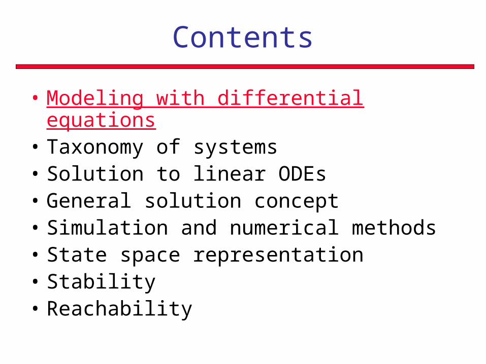
Contents
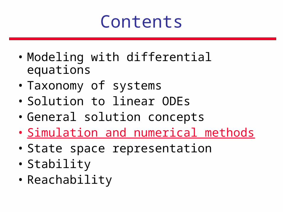
• Modeling with differential equations• Taxonomy of systems• Solution to linear ODEs• General solution concept• Simulation and numerical methods• State space representation• Stability• Reachability

Physical systems
Resistor Inductor Capacitor
Damper Mass Spring
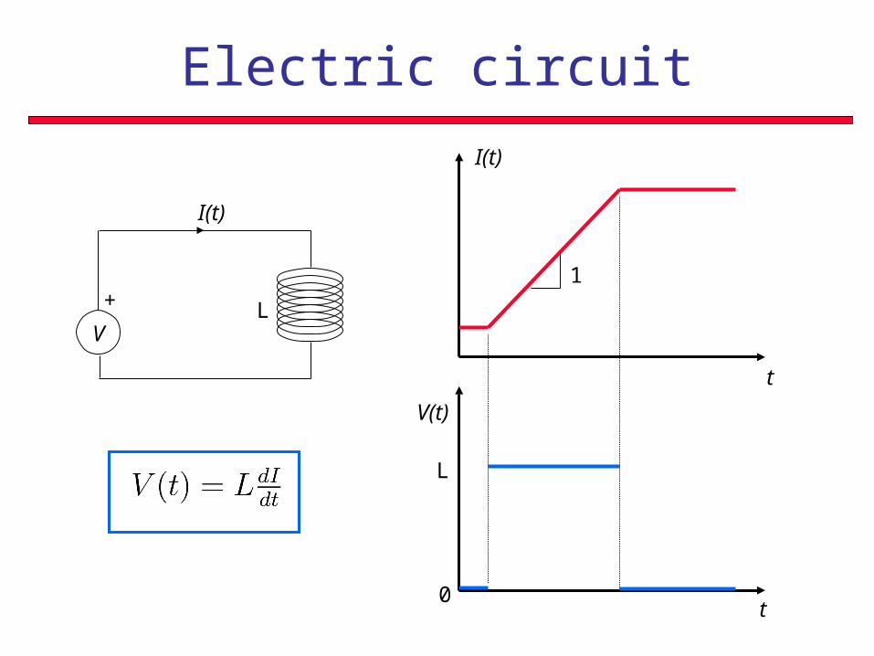
Electric circuit
V
+
I(t)
1
0
t
I(t)
V(t)
t
L
L
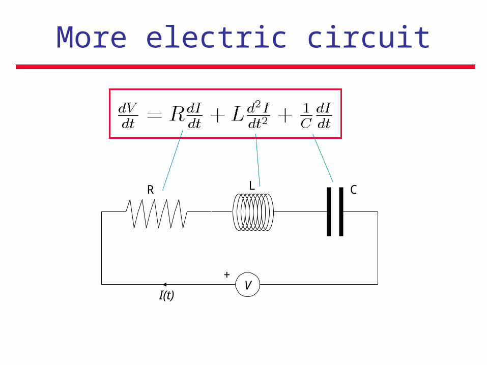
More electric circuit
VI(t)
+
R L C

A pendulum
Mg
r

Contents
• Modeling with differential equations• Taxonomy of systems• Solution to linear ODEs• General solution concept• Simulation and numerical methods• State space representation• Stability• Reachability
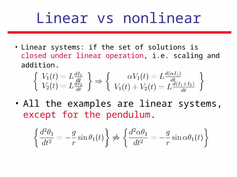
Linear vs nonlinear
• Linear systems: if the set of solutions is closed under linear operation, i.e. scaling and addition.
• All the examples are linear systems, except for the pendulum.

Time invariant vs time varying
• Time invariant: the set of solutions is closed under time shifting.
• Time varying: the set of solutions is not closed under time shifting.

Autonomous vs non-autonomous
• Autonomous systems: given the past of the signals, the future is already fixed.
• Non-autonomous systems: there is possibility for input, non-determinism.
Contents
• Modeling with differential equations• Taxonomy of systems• Solution to linear ODEs• General solution concept• Simulation and numerical methods• State space representation• Stability• Reachability

Techniques for autonomous systems

Techniques for non-autonomous systems
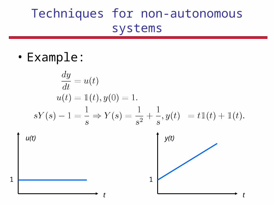
Techniques for non-autonomous systems
• Example:
1
u(t)
t
1
y(t)
t

Contents
• Modeling with differential equations• Taxonomy of systems• Solution to linear ODEs• General solution concepts• Simulation and numerical methods• State space representation• Stability• Reachability

Solution concepts

Example of weak solution
Contents
• Modeling with differential equations• Taxonomy of systems• Solution to linear ODEs• General solution concepts• Simulation and numerical methods• State space representation• Stability• Reachability

Simulation methods
x(t)x[1] x[2]x[3]
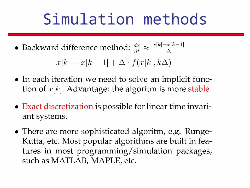
Simulation methods
Contents
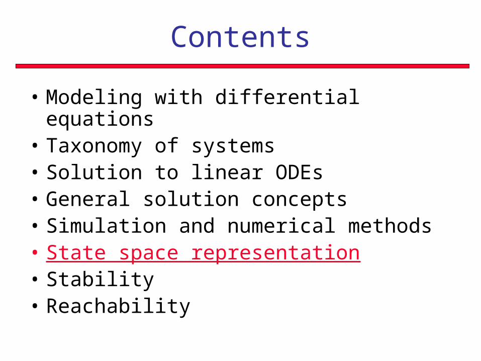
• Modeling with differential equations• Taxonomy of systems• Solution to linear ODEs• General solution concepts• Simulation and numerical methods• State space representation• Stability• Reachability

State space representation• One of the most important representations of
linear time invariant systems.

State space representation

Solution to state space rep.
Solution:

Exact discretization of autonomous systems
x(t)x[1]
x[2]
x[3]
t

Contents
• Modeling with differential equations• Taxonomy of systems• Solution to linear ODEs• Simulation and numerical methods• State space representation• Stability• Reachability• Discrete time systems

Stability of LTI systems

Stability of nonlinear systems
p p
stable
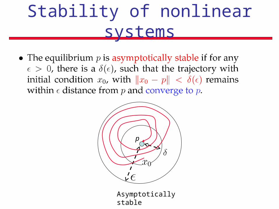
Stability of nonlinear systems
p
Asymptotically stable

Lyapunov functions

Contents
• Modeling with differential equations• Taxonomy of systems• Solution to linear ODEs• General solution concept• Simulation and numerical methods• State space representation• Stability• Reachability

Reachability

Reachability of linear systems