Spring, 2013C.-S. Shieh, EC, KUAS, Taiwan1 Heuristic Optimization Methods A Tutorial on...

Spring, 2013 C.-S. Shieh, EC, KUAS, Taiwan 1

Heuristic Optimization Methods

A Tutorial on Meta-Heuristics for Optimization

Chin-Shiuh Shieh


Abstract

• Nature has inspired computing and engineering researchers in many different ways.

• Natural processes have been emulated through a variety of techniques including genetic algorithms, ant systems and particle swarm optimization, as computational models for optimization.


Introduction

• Optimization problems arise from almost every field ranging from academic research to industrial application.

• Meta-heuristics, such as genetic algorithms, particle swarm optimization and ant colony systems, have received increasing attention in recent years for their interesting characteristics and their success in solving problems in a number of realms.

• Detailed implementations in C are given.


Introduction (cont)


Genetic Algorithms

• Darwin's theory of natural evolution– Creatures compete with each other for limited

resources.– Those individuals that survive in the competition have

the opportunity to reproduce and generate descendants.

– Exchange of genes by mating may result in superior or inferior descendants.

– The process of natural selection eventually filtering out inferior individuals and retain those adapted best to their environment.


Genetic Algorithms (cont)

• Genetic algorithms– introduced by J. Holland in 1975– work on a population of potential solutions, in

the form of chromosomes (染色體 ),– try to locate a best solution through the proce

ss of artificial evolution, which consist of repeated artificial genetic operations, namely

• Evaluation• Selection• Crossover and mutation


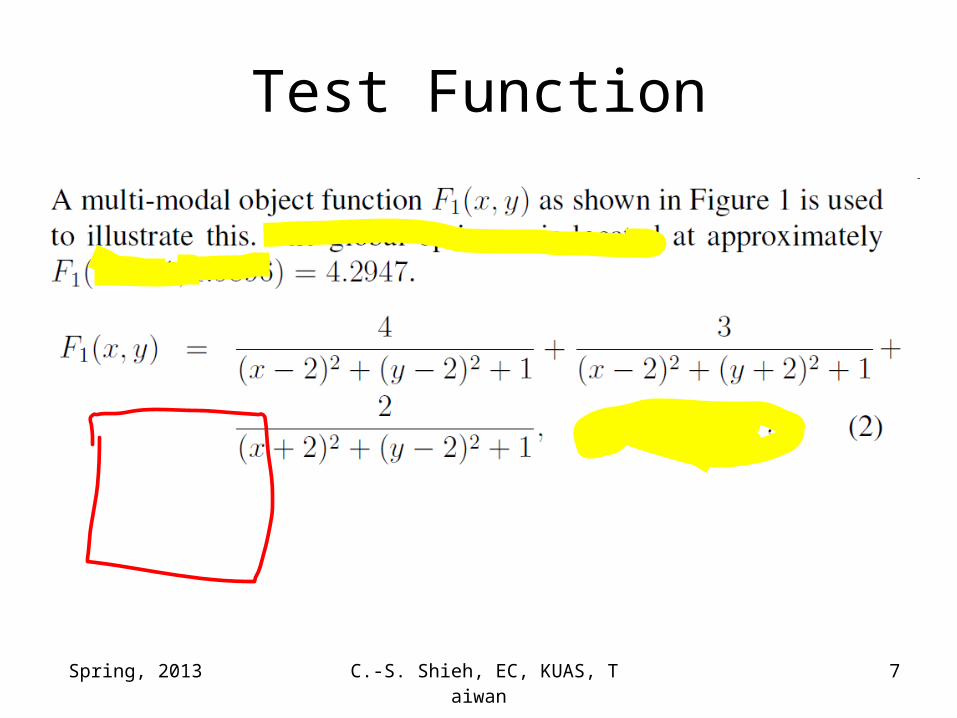
Test Function


Test Function (cont)


Representation

• Select an adequate coding scheme to represent potential solutions in the search space in the form of chromosomes.– binary string coding for numerical optimization– expression trees for genetic programming– city index permutation for the travelling

salesperson problem


Representation (cont)

• We use a typical binary string coding for the test function F1

– Each genotype has 16 bits to encode an independent variable.

– A decoding function maps the 65536 possible combinations of b15 … b0 onto the range [-5,5) linearly.

– A chromosome is then formed by cascading genotypes for each variable.

– With this coding scheme, any 32 bit binary string stands for a legal point in the problem domain.



• 1110101110110011| 0010110011111010

• (1110101110110011)2=(60339)10

• x = 60339/216*10-5=4.207000732421875

• (0010110011111010)2=(11514)10

• y = 11514/216*10-5=-3.24310302734375


Population Size

• The choice of population size, N, is a tradeoff between solution quality and computation cost.

• A larger population size will maintain higher genetic diversity and therefore a higher possibility of locating global optimum, however, at a higher computational cost.


Operation of Genetic Algorithms

Step 1 Initialization

Step 2 Evaluation

Step 3 Selection

Step 4 Crossover

Step 5 Mutation

Step 6 Termination Checking

Go to Step 2 if not terminated



• Each bit of all N chromosomes in the population is randomly set to 0 or 1.

• This operation in effect spreads chromosomes randomly into the problem domains.

• Whenever possible, it is suggested to incorporate any a priori knowledge of the search space into the initialization process to endow the genetic algorithm with a better starting point.


Step 2 Evaluation


Step 3 Selection


• f1=1, f2=2, f3=3

• For SF=1, Pr(c2 be selected) =2/(1+2+3)=0.33

• For SF=3, Pr(c2 be selected) =23/(13+23+33)=0.22


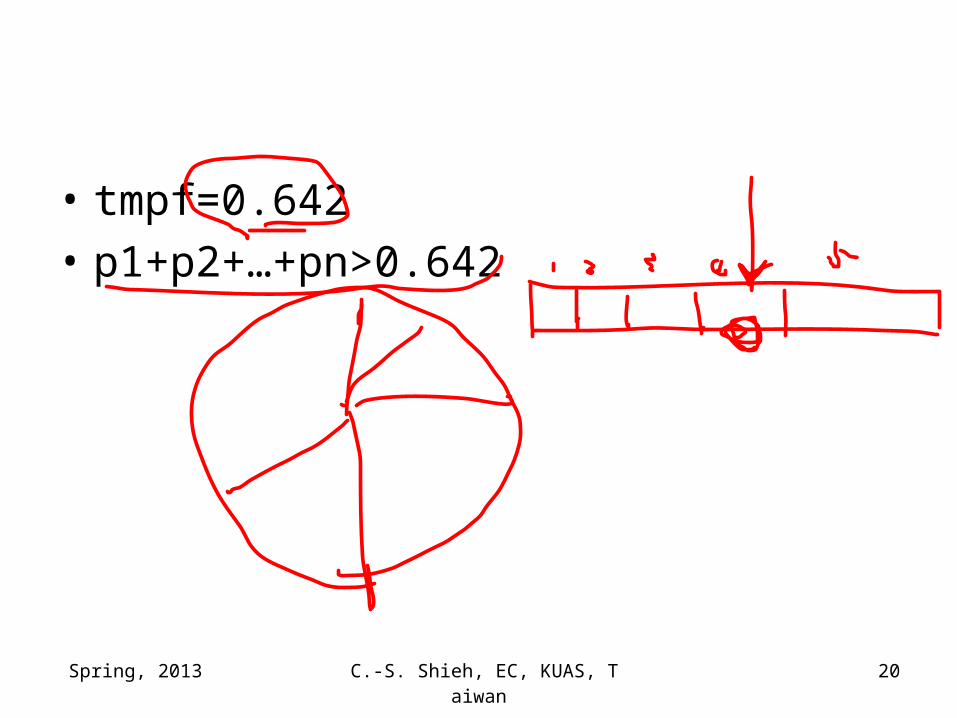
• f1=1, f2=2,f3=3,f4=4,f5=5• SF=1• p1=1/(1+2+3+4+5)=1/15=0.067• p2=2/15=0.133• p3=3/15=0.200• p4=4/15=0.267• p5=5/15=0.333• p1+p2+p3+p4+p5=1


• tmpf=0.642

• p1+p2+…+pn>0.642


Step 3 Selection (cont)

• As a result, better chromosomes will have more copies in the new population, mimicking the process of natural selection.

• In some applications, the best chromosome found is always retained in the next generation to ensure its genetic material remains in the gene pool.


Step 4 Crossover

• Pairs of chromosomes in the newly generated population are subject to a crossover (or swap) operation with probability PC, called Crossover Rate.

• The crossover operator generates new chromosomes by exchanging genetic material of pair of chromosomes across randomly selected sites, as depicted in Figure 3.


Step 4 Crossover (cont)


Step 4 Crossover (cont)

• Similar to the process of natural breeding, the newly generated chromosomes can be better or worse than their parents. They will be tested in the subsequent selection process, and only those which are an improvement will thrive.


Step 5 Mutation

• After the crossover operation, each bit of all chromosomes are subjected to mutation with probability PM, called the Mutation Rate.

• Mutation flips bit values and introduces new genetic material into the gene pool.


Step 5 Mutation (cont)

• This operation is essential to avoid the entire population converging to a single instance of a chromosome, since crossover becomes ineffective in such situations.

• In most applications, the mutation rate should be kept low and acts as a background operator to prevent genetic algorithms from random walking.



• Genetic algorithms repeat Step 2 to Step 5 until a given termination criterion is met, such as pre-defined number of generations or quality improvement has failed to have progressed for a given

• number of generations.

• Once terminated, the algorithm reports the best chromosome it found.


Experiment Results

• The global optimum is located at approximately F1(1.9931,1.9896) = 4.2947.

• With a population of size 10, after 20 generations, the genetic algorithm was capable of locating a near optimal solution at F1(1.9853,1.9810) = 4.2942.

• Due to the stochastic nature of genetic algorithms, the same program may produce a different results on different machines.


Experiment Results (cont)


Discussions

• Important characteristics providing robustness– They search from a population of points rather

than a single point.– The use the object function directly, not their

derivative.– They use probabilistic transition rules, not

deterministic ones, to guide the search toward promising region.


Discussions (cont)

• In effect, genetic algorithms maintain a population of candidate solutions and conduct stochastic searches via information selection and exchange.

• It is well recognized that, with genetic algorithms, near-optimal solutions can be obtained within justified computation cost.


Discussions (cont)

• However, it is difficult for genetic algorithms to pin point the global optimum.

• In practice, a hybrid approach is recommended by incorporating gradient-based or local greedy optimization techniques.

• In such integration, genetic algorithms act as course-grain optimizers and gradient-based method as fine-grain ones.


Discussions (cont)

• The power of genetic algorithms originates from the chromosome coding and associated genetic operators.

• It is worth paying attention to these issues so that genetic algorithms can explore the search space more efficiently.


Discussions (cont)

• The selection factor controls the discrimination between superior and inferior chromosomes.

• In some applications, more sophisticated reshaping of the fitness landscape may be required.

• Other selection schemes (Whitley 1993), such as rank-based selection, or tournament selection are possible alternatives for the controlling of discrimination.


Variants

• Parallel genetic algorithms

• Island-model genetic algorithms– maintain genetic diversity by splitting a

population into several sub-populations, each of them evolves independently and occasionally exchanges information with each other


Variants (cont)

• Multiple-objective genetic algorithms– attempt to locate all near-optimal solutions by

careful controlling the number of copies of superior chromosomes such that the population will not be dominated by the single best chromosome


Variants (cont)

• Co-evolutionary systems– have two or more independently evolved

populations. The object function for each population is not static, but a dynamic function depends on the current states of other populations.

– This architecture vividly models interaction systems, such as prey and predator, virus and immune system.


Particle Swarm Optimization

• Some social systems of natural species, such as flocks of birds and schools of fish, possess interesting collective behavior.

• In these systems, globally sophisticated behavior emerges from local, indirect communication amongst simple agents with only limited capabilities.


Particle Swarm Optimization (cont)

• Kennedy and Eberthart (1995) realized that an optimization problem can be formulated as that of a flock of birds flying across an area seeking a location with abundant food.

• This observation, together with some abstraction and modification techniques, led to the development of a novel optimization technique – particle swarm optimization.



• Particle swarm optimization optimizes an object function by conducting a population-based search.

• The population consists of potential solutions, called particles, which are a metaphor of birds in flocks.

• These particles are randomly initialized and freely fly across the multi-dimensional search space.



• During flight, each particle updates its velocity and position based on the best experience of its own and the entire population.

• The updating policy will drive the particle swarm to move toward region with higher object value, and eventually all particles will gather around the point with highest object value.



• The velocity and position of all particles are randomly set to within pre-specified or legal range.


Step 2 Velocity Updating


Step 2 Velocity Updating (cont)

• The inclusion of random variables endows the particle swarm optimization with the ability of stochastic searching.

• The weighting factors, c1 and c2, compromises the inevitable tradeoff between exploration and exploitation.

• After the updating, vi should be checked and clamped to pre-specified range to avoid violent random walking.


Step 3 Position Updating


Step 4 Memory Updating


Test Function


Experiment Results


Distribution of Particles


Distribution of Particles (cont)


Variants

• A discrete binary version of the particle swarm optimization algorithm was proposed by Kennedy and Eberhart (1997).

• Shi and Eberhart (2001) applied fuzzy theory to particle swarm optimization algorithm.

• Successfully incorporated the concept of co-evolution in solving min-max problems (Shi and Krohling 2002).

• (Chu et al. 2003) have proposed a parallel architecture with communication mechanisms for information exchange among independent particle groups, in which solution quality can be significantly improved.


Ant System

• Inspired by the food-seeking behavior of real ants, Ant Systems, attributable to Dorigo et al. (Dorigo et al. 1996), has demonstrated itself to be an efficient, effective tool for combinatorial optimization problems.


Ant System (cont)

• In nature, a real ant wandering in its surrounding environment will leave a biological trace, called pheromone, on its path.

• The intensity of left pheromone will bias the path-taking decision of subsequent ants.

• A shorter path will possess higher pheromone concentration and therefore encourage subsequent ants to follow it.

• As a result, an initially irregular path from nest to food will eventually contract to a shorter path.


Ant System (cont)

• With appropriate abstraction and modification, this observation has led to a number of successful computational models for combinatorial optimization.


Test Problem

• Travelling Salesman Problem

• In the TSP, a travelling salesman problem is looking for a route which covers all cities with minimal total distance.


Test Problem (cont)


Operation

• Suppose there are n cities and m ants.• The entire algorithm starts with initial pheromone

intensity set to τ0 on all edges. • In every subsequent ant system cycle, or episod

e, each ant begins its trip from a randomly selected starting city and is required to visit every city exactly once (a Hamiltonian Circuit).

• The experience gained in this phase is then used to update the pheromone intensity on all edges.



• Initial pheromone intensities on all edges are set to τ0.


Step 2 Walking phase

• In this phase, each ant begins its trip from a randomly selected starting city and is required to visit every city exactly once.

• When an ant, the k-th ant for example, is located at city r and needs to decide the next city s, the path-taking decision is made stochastically based on the following probability function:


Step 2 Walking phase (cont)


Step 2 Walking phase (cont)

• According to Equation 6, an ant will favor a nearer city or a path with higher pheromone intensity.

• β is parameter used to control the relative weighting of these two factors.

• During the circuit, the route made by each ant is recorded for pheromone updating in step 3.

• The best route found so far is also tracked.


Step 3 Updating phase


Step 3 Updating phase (cont)

• The updated pheromone intensities are then used to guide the path-taking decision in the next ant system cycle.

• It can be expected that, as the ant system cycle proceeds, the pheromone intensities on the edges will converge to values reflecting their potential for being components of the shortest route.

• The higher the intensity, the more chance of being a link in the shortest route, and vice visa.



• Ant systems repeat Step 2 to Step 3 until certain termination criteria are met– A pre-defined number of episodes is

performed– the algorithm has failed to make

improvements for certain number of episodes.

• Once terminated, ant system reports the shortest route found.


Experiment Results

• Figure 6 reports a found shortest route of length 3.308, which is the truly shortest route validated by exhaustive search.


Experiment Results (cont)


Ant Colony System

• A close inspection on the ant system reveals that the heavy computation required may make it prohibitive in certain applications.

• Ant Colony Systems was introduced by Dorigo et al. (Dorigo and Gambardella 1997) to remedy this difficulty.


Ant Colony System (cont)

• Ant colony systems differ from the simpler ant system in the following ways:– Explicit control on exploration and exploitation– Local updating– Count only the shortest route in global

updating


Explicit control on exploration and exploitation

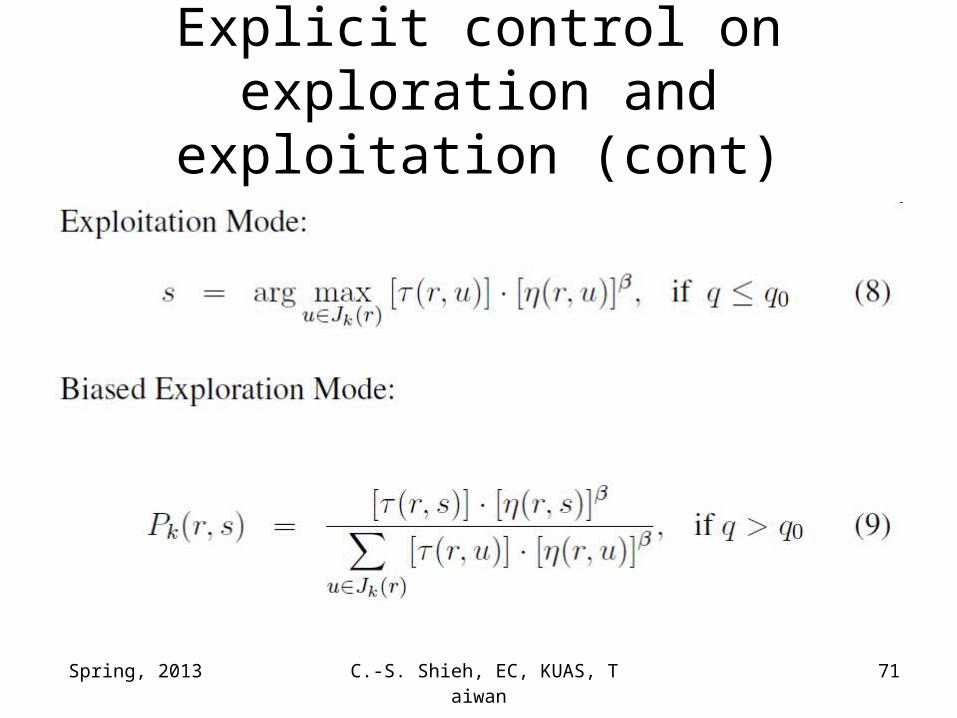
• When an ant is located at city r and needs to decide the next city s, there are two modes for the path-taking decision, namely exploitation and biased exploration.

• Which mode to be used is governed by a random variable 0 < q < 1,


Explicit control on exploration and exploitation (cont)


Local updating

• A local updating rule is applied whenever a edge from city r to city s is taken:


Count only the shortest route in global updating

• As all ants complete their circuits, the shortest route found in the current episode is used in the global updating rule:


Discussion

• In some respects, the ant system has implemented the idea of emergent computation – a global solution emerges as distributed agents performing local transactions, which is the working paradigm of real ants.

• The success of ant systems in combinatorial optimization makes it a promising tool for dealing with a large set of problems in the NP-complete class (Papadimitriou and Steiglitz 1982).


Variants

• In addition, the work of Wang and Wu (Wang and Wu 2001) has extended the applicability of ant systems further into continuous search space.

• Chu et al. (2003) have proposed a parallel ant colony system, in which groups of ant colonies explore the search space independently and exchange their experiences at certain time intervals.

Spring, 2013C.-S. Shieh, EC, KUAS, Taiwan1 Heuristic Optimization Methods A Tutorial on...

Documents

Transcript of Spring, 2013C.-S. Shieh, EC, KUAS, Taiwan1 Heuristic Optimization Methods A Tutorial on...