Spreadsheet Fluid Dynamics forAeronautical Course Problems*

ETSUO MORISHITA, YOHEI IWATA, KENTARO YUKI and HARUHIKO YOSHIDAGraduate School of Engineering, Department of Aeronautics and Astronautics, University of Tokyo, 7-3-1,Hongo, Bunkyo-ku, Tokyo, 113-8656, Japan. E-mail: morisita@fanno.t.u-tokyo.ac.jp

Computational Fluid Dynamics is now used daily in scientific and engineering practices. Thecomputations themselves are now based on commercially available software. Personal computersare widely utilized elsewhere these days and many people are using spreadsheets as well as wordprocessors. It is now well known to the scientific and engineering communities that spreadsheets canbe used, not only for statistics and data processing calculations, but also for matrix inverse,iteration in a finite difference equation, and for special functions of mathematics. This situationallows us to realize SFD, i.e., Spreadsheet Fluid Dynamics. The authors have demonstrated thatthe fluid dynamics equations could be solved efficiently by using a spreadsheet. The cells in thespreadsheet are viewed as either natural grids in CFD or elements of a matrix. The computationaldomain corresponds to the real physical shape and/or the computational space by grid generation.The result can be visualized on the same spreadsheet with inherent graphics. The pre- and post-processors are all in one in SFD.

AUTHOR'S QUESTIONNAIRE

1. The paper describes software/hardware/simula-tion tools which are suitable for students ofthe following courses: Aerodynamics, FluidMechanics, Gas Dynamics, Heat and MassTransfer.

2. The level involved is for undergraduates (thirdand fourth year) and masters degree students.

3. New material covered by this paper includesspreadsheet applications to general aero-dynamic and/or fluid dynamic problems fromconventional calculations to the NS finitedifference solutions.

4. The material is presented by means of classroomdemonstration and homework assignments;samples are obtained via the Internet.

5. The following texts accompany the presentedmaterial:Misner, C. W. & Cooney, P. J., SpreadsheetPhysics, Addison-Wesley, 1991.Gottfried, B. S., Spreadsheet Tools forEngineers, McGraw-Hill, 1996.Walkenbach, J., Excel 97 Bible, IDG Books,1996.Morishita, E., Spreadsheet fluid dynamics, J.Aircraft, 36, 4, 1999, pp. 720±723.Morishita, E., et al., AIAA Paper 2000-0804,38th Aerospace Sciences.

6. SFD is now being tested in the classroom(potential flow and gas dynamics). Findings todate:± almost free from computational literacy

problems;

± concentration on the subjects themselves;± quick understanding and progress in the

numerical procedure;± animation by graphics very useful.

7. People who are not specialized in the numericalmethod are also benefited from this technique.A lengthy program can be replaced by a verysimple spreadsheet in some cases.

NOMENCLATURE

A � coefficient matrixb � vectorCd � drag coefficientCl � lift coefficientCm � moment coefficientCp � pressure coefficientCQ � torque coefficientCT � thrust coefficientc � chordK � transonic similarity parameterL � lift, lengthl � panel lengthM � Mach numberm0 � lift slopeN � numbers of bladesn � rpsp � pressureR � propeller radius, residualr � radiuss � distanceu; v � velocity componentV � velocity vectorV � flight velocity* Accepted 20 August 2000.

294

Int. J. Engng Ed. Vol. 17, No. 3, pp. 294±311, 2000 0949-149X/91 $3.00+0.00Printed in Great Britain. # 2000 TEMPUS Publications.

Vi � induced velocityVR � relative velocityx; y � coordinatez � complex variable

� � angle of attack� � blade pitch angle� � potential, effective-pitch angleÿ � circulation � vortex strength, specific heat ratio� � efficiency� � density� � solidity (� Nc=��R�)� � thickness ratio! � angular velocity, relaxation factor�; � � transformed coordinate� � complex variable

suffixescal � calculationc.p. � center of pressureexp � experimenti � inducedi; j � i; j nodeinf � infinityn � n-th iterationth � theoretical value0 � zero lift, leading edge2-D � two-dimensional1 � infinity

INTRODUCTION

THE SPREADSHEET is a very powerful engin-eering tool and it is used widely for scientific andengineering calculations [1±4]. One of the authorsproposed using a spreadsheet for aerodynamicsproblems [4]. The emergence of computationalfluid dynamics enables us to obtain detailed infor-mation on flow fields. Our experience in comput-ing was that it took a very long time to learncomputer languages and it was sometimes veryhard to obtain proper results in a limited time.The spreadsheet, however, is rather easy to use andalmost instantaneous numerical simulations arepossible.

A Spreadsheet Fluid Dynamics (SFD) functionis to solve aerodynamic and fluid dynamicsproblems by using a spreadsheet. There are typicallythree types of SFD:

Type I: conventional spreadsheet calculation,including the use of engineering func-tions.

Type II: matrix inverse and vector product.Type III: iteration in a finite difference equation.

Type I calculation was used for a propeller calcula-tion [5, 6] in this paper. This method can be usedfor complex potential calculations like a potentialflow around a circular cylinder [7] and an airfoil.Conventional spreadsheet calculations can alsohandle the numerical integration of ordinarydifferential equations by the Runge-Kutta

method so that the self-similar boundary layerequation [8±10] is solved.

In Type II, matrix inversion by spreadsheet isa very powerful function for engineering appli-cations. In aeronautical problems, the panelmethod [11, 12] involves the solution of linearsimultaneous equations. The two-dimensionalsolution is obtained instantly by a spreadsheet.The choice of airfoil is also very easy. The numeri-cal technique for a three-dimensional wing is alsopossible. The lifting line theory [12, 13] and thevortex lattice methods [14] both involve the matrixinverse and these types of problems are solvedquite easily.

Type III seems to be the most important one inSFD. The iteration and the circular referencefunctions of spreadsheets [3] make it possible tosolve finite difference equations. The cells in thespreadsheet are recognized as grids in CFD. Theprocedure used to solve the transonic smalldisturbance equation [15±18] is presented indetail in the present paper. The Laplace [4], theEuler [19±21], and the Navier-Stokes equationscan be handled by SFD III. The classical methodof characteristics [22±24] is also included inthis category. Fluid dynamic instability [4, 25±29]is also one of the interesting subjects relating toSFD III.

SFD I ± CONVENTIONAL CALCULATION

SFD Type I is when the conventional spread-sheet calculation is applied to aerodynamic andfluid dynamic problems. Here, we introduce theprocedureusedtocalculatepropellercharacteristics.

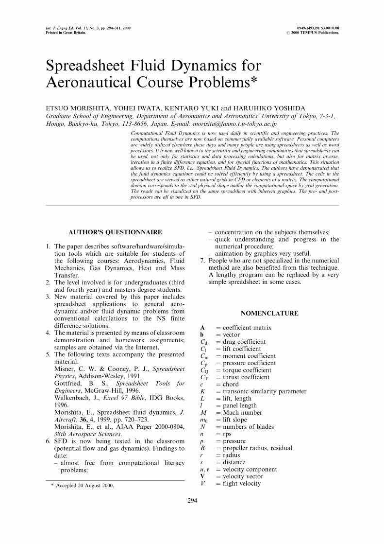
The characteristics of a propeller can bepredicted rather well by the classical momentum-blade element theory [5]. The aerodynamic perfor-mances at each radius are compiled to obtainits complete characteristics. Figure 1 shows thecross-sectional view of the propeller blade [5].

The sectional lift, defined as normal to the localflow direction is given by:

dL � 1

2�V 2

RClcdr �1�

Therefore, the potential thrust componentbecomes:

dT � dL cos��� �i� � 1

2�V2

RClcdr cos��� �i��2�

The momentum theory predicts the inducedvelocity in the far wake and has a value of2Vi cos��� �i�. The momentum change acrossthe propeller must be equal to equation (2), i.e.

dT � 2�dr��V � Vi cos��� �i�� � 2Vi cos��� �i��3�

Spreadsheet Fluid Dynamics for Aeronautical Course Problems 295

From equations (2) and (3), the induced angle ofattack �i in Fig. 1 is derived as follows [5]:

�i � � ÿ �ÿ �0

1� 8r

R

sin�

�m0

�4�

Equation (4) is the first-order approximation andthe more accurate second-order approximation isalso obtainable. From equation (4), we obtain thesectional thrust dT and the torque dQ of thepropeller as follows:

dT �N�dL cos��� �i� ÿ dD sin��� �i�� �5�dQ �N�rdL sin��� �i� � rdD cos��� �i�� �6�

Although we assume the potential flow to derivean induced angle of attack �i, we include theviscous effect in equations (5) and (6). We canshow that equations (5) and (6) become [5]:

dCT

dx� �

2cNx2

8R

cos2 �i

cos2 �

��Cl cos��� �i� ÿ Cd sin��� �i�� � �3�x2

8�T

�7�dCQ

dx� �

2cNx3

16R

cos2 �i

cos2 �

��Cl cos��� �i� � Cd sin��� �i�� � �3�x3

16�Q

�8�Equations (7) and (8) can be numerically inte-grated (actually summed) by a spreadsheet.

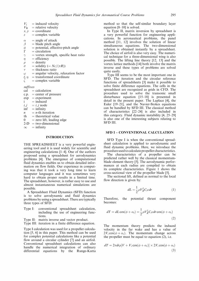
The theory was compared to the experiment,R & M 829 No. 5 blade shape, a 4-blade woodenpropeller [6]. We opened a spreadsheet and firstspecified the advance ratio V=nD as shown in cellC12 in Table 1. The value was chosen from Ref. 6for the comparison. Six radial locations (row 14in Table 1) were chosen after the R & M 829 [6].The chord c, the zero-lift angle of attack �0

and the number of blades N were obtained fromRef. 6 (rows 15-18 in Table 1). We calculated� � V=�R!� in row 19 of Table 1. The solidity� is calculated in row 20. The blade angles �were specified from Ref. 6 (rows 21 and 22 inTable 1).

The effective-pitch angle � was calculatedfrom:

� � tanÿ1 V

r!� tanÿ1 �

x�9�

For the cell C23, equation (9) was expressed:=ATAN(C19/C14). The two-dimensional airfoilcharacteristics were employed in the momentum-blade-element theory and the lift slope m0 wasassumed to be 2� in the present calculation(row 25 in Table 1). The induced angle ofattack �i was the obtained from equation (4)(rows 26 and 27 in Table 1). The sectional liftcoefficient was then calculated as follows (row 28in Table 1):

Cl � m0�� ÿ �ÿ �0 ÿ �i� �10�We assumed the sectional drag coefficient Cd tobe 0.015 to take the viscous effect into account(row 29 in Table 1). We then calculated �T and�Q in equations (7) and (8) (rows 30 and 31 inTable 1). The thrust and torque radial gradientswere also obtained from equations (7) and (8)(rows 32 and 33 in Table 1 ). The torque andtrust coefficients were calculated approximatelyby:

CT �X dCT

dx�x �11�

CQ �X dCQ

dx�x �12�

where �x � 0:15 was employed for simplicity(C35 and C36 in Table 1). In C35, the spread-sheet command: =SUM(C32:H32)*0.15, wasemployed to calculate equations (11). Equation

Fig. 1. Propeller section.

Table 1. Propeller calculation (R&M829 4-blade woodenpropeller [6])

E. Morishita et al.296

(12) was calculated similarly. The efficiency of thepropeller was calculated by (C37 in Table 1):

� � CT

2�CQ

V

nD�13�

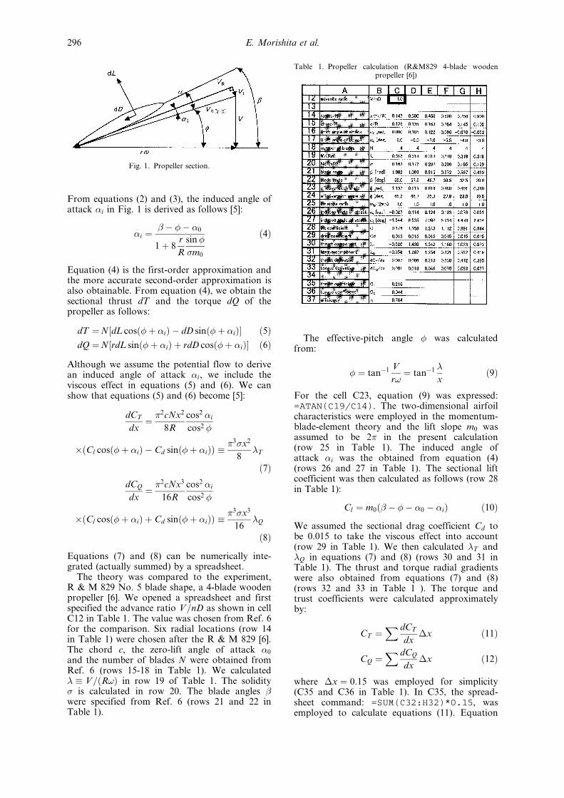
We repeated the calculation for each experimentaladvance ratio [6] to get a comparison and theresults are shown in Fig. 2. Although a smalldifference is observed at a smaller advance ratioV=nD, the agreement is quite satisfactory in spiteof the simplicity of the theory. The difference at thesmaller advance ratio may be attributed to theconstant sectional drag coefficient and the first-order approximation in the induced angle ofattack. We recognize the negative thrust near theroot for the given advance ratio in Table 1 and thishappens at the off-peak efficiency operation. Thevariable-pitch propeller can minimize this type ofloss and keep the optimum efficiency at a widerange of the advance ratio. The thrust and torqueare both reduced at higher advance ratios becausethe average effective angle of attack is alsoreduced. When we further increase the advanceratio, we finally reach the point where neitherthrust nor torque is produced.

SFD II ± MATRIX INVERSE

One of the most convenient tools of spread-sheets is the function of matrix inverse, where acommand `MINVERSE' is employed [2]. Thepanel method [11, 12 pp. 260±288] is a typicalexample of SFD Type II.

The panel method is efficient for handlingthe lifting problem of a two-dimensional airfoil.

We use the vortex-based panel method and thepotential is obtained for a flow around a two-dimensional airfoil as follows [11, 12]:

��x; y� �U1�x cos�� y tan��

�XN

j�1

�Panel j

ÿ �s�2�

�ds �14�

where the linear vortex distribution [11, 12] isassumed along a panel in the present calculation,i.e.

�s� � j � � j�1 ÿ j� s

lj�15�

� � tanÿ1 yÿ y�s�xÿ x�s� �16�

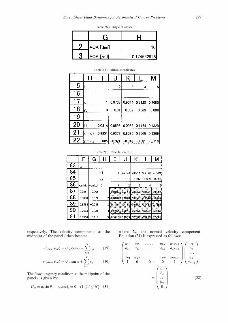
We introduced the spreadsheet procedure tohandle the panel method. First we specified theangle of attack as 10 degrees, and we converted itto radians as (H3 in Table 2(a)): =RADIANS(H2).We then specified the coordinate �xj ; yj� of the j-thpanel of the airfoil. The initial j � 1±5 is shownTable 2(b). A Karman-Trefftz airfoil [11] was usedbecause the exact analytical solution was available.The transformation is given by:

� ÿ 1

� � 1� zÿ 1

z� 1

� �k

�17�

The complex number represents a base circle thathas a center at z0 � �ÿ0:1; 0:1� and passes (1,0).k � 1:7 is in the present example. We employed 40panels (i.e. 41 nodes) on the airfoil and thecoordinates were actually obtained from theequally spaced points on the base circle. Care must

Fig. 2. Propeller characteristics (R&M829 4-blade wooden propeller [6]): (a) Thrust coefficient CT; (b) Torque coefficient CQ;(c) Efficiency �.

Spreadsheet Fluid Dynamics for Aeronautical Course Problems 297

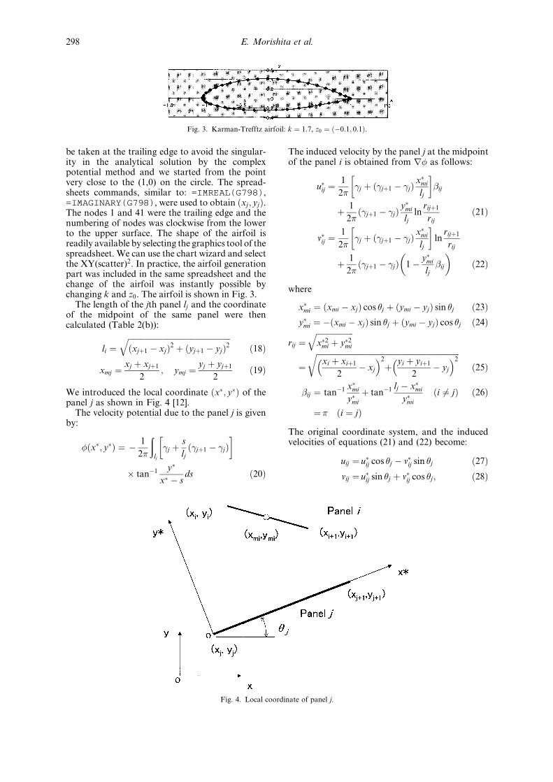
be taken at the trailing edge to avoid the singular-ity in the analytical solution by the complexpotential method and we started from the pointvery close to the (1,0) on the circle. The spread-sheets commands, similar to: =IMREAL(G798),=IMAGINARY(G798), were used to obtain �xj; yj�.The nodes 1 and 41 were the trailing edge and thenumbering of nodes was clockwise from the lowerto the upper surface. The shape of the airfoil isreadily available by selecting the graphics tool of thespreadsheet. We can use the chart wizard and selectthe XY(scatter)2. In practice, the airfoil generationpart was included in the same spreadsheet and thechange of the airfoil was instantly possible bychanging k and z0. The airfoil is shown in Fig. 3.

The length of the jth panel lj and the coordinateof the midpoint of the same panel were thencalculated (Table 2(b)):

li �������������������������������������������������������xj�1 ÿ xj�2 � �yj�1 ÿ yj�2

q�18�

xmj � xj � xj�1

2; ymj � yj � yj�1

2�19�

We introduced the local coordinate �x�; y�� of thepanel j as shown in Fig. 4 [12].

The velocity potential due to the panel j is givenby:

��x�; y�� � ÿ 1

2�

�lj

j � s

lj� j�1 ÿ j�

� �� tanÿ1 y�

x� ÿ sds �20�

The induced velocity by the panel j at the midpointof the panel i is obtained from r� as follows:

u�ij �1

2� j � � j�1 ÿ j� x

�mi

lj

� ��ij

� 1

2�� j�1 ÿ j� y

�mi

ljln

rij�1

rij�21�

v�ij �1

2� j � � j�1 ÿ j� x

�mi

lj

� �ln

rij�1

rij

� 1

2�� j�1 ÿ j� 1ÿ y�mi

lj�ij

� ��22�

where

x�mi � �xmi ÿ xj� cos �j � �ymi ÿ yj� sin �j �23�y�mi � ÿ�xmi ÿ xj� sin �j � �ymi ÿ yj� cos �j �24�

rij ��������������������x�2mi � y�2mi

q�

��������������������������������������������������������������������������xi � xi�1

2ÿ xj

� �2

� yi � yi�1

2ÿ yj

� �2r

�25�

�ij � tanÿ1 x�mi

y�mi

� tanÿ1 lj ÿ x�mi

y�mi

�i 6� j� �26�

� � �i � j�The original coordinate system, and the inducedvelocities of equations (21) and (22) become:

uij � u�ij cos �j ÿ v�ij sin �j �27�vij � u�ij sin �j � v�ij cos �j ; �28�

Fig. 4. Local coordinate of panel j.

Fig. 3. Karman-Trefftz airfoil: k � 1:7, z0 � �ÿ0:1; 0:1�.

E. Morishita et al.298

respectively. The velocity components at themidpoint of the panel i then become:

ui�xmi; ymi� �U1 cos��XN

j�1

uij �29�

vi�xmi; ymi� �U1 sin��XN

j�1

vij �30�

The flow tangency condition at the midpoint of thepanel i is given by:

Uni � ui sin �i ÿ vi cos �i � 0 �1 � i � N� �31�

where Uni the normal velocity component.Equation (31) is expressed as follows:

a11 a12 . . . . . . a1N a1N�1

a21 a22 . . . . . . a2N a2N�1

aN1 aN2 aNN aNN�1

1 0 . . . 0 . . . 0 1

0BBBB@1CCCCA

1

2

. . . N

N�1

0BBBB@1CCCCA

�

b1

b2

. . .bN

0

0BBBB@1CCCCA �32�

Table 2(a). Angle of attack

Table 2(b). Airfoil coordinates

Table 2(c). Calculation of ri j

Spreadsheet Fluid Dynamics for Aeronautical Course Problems 299

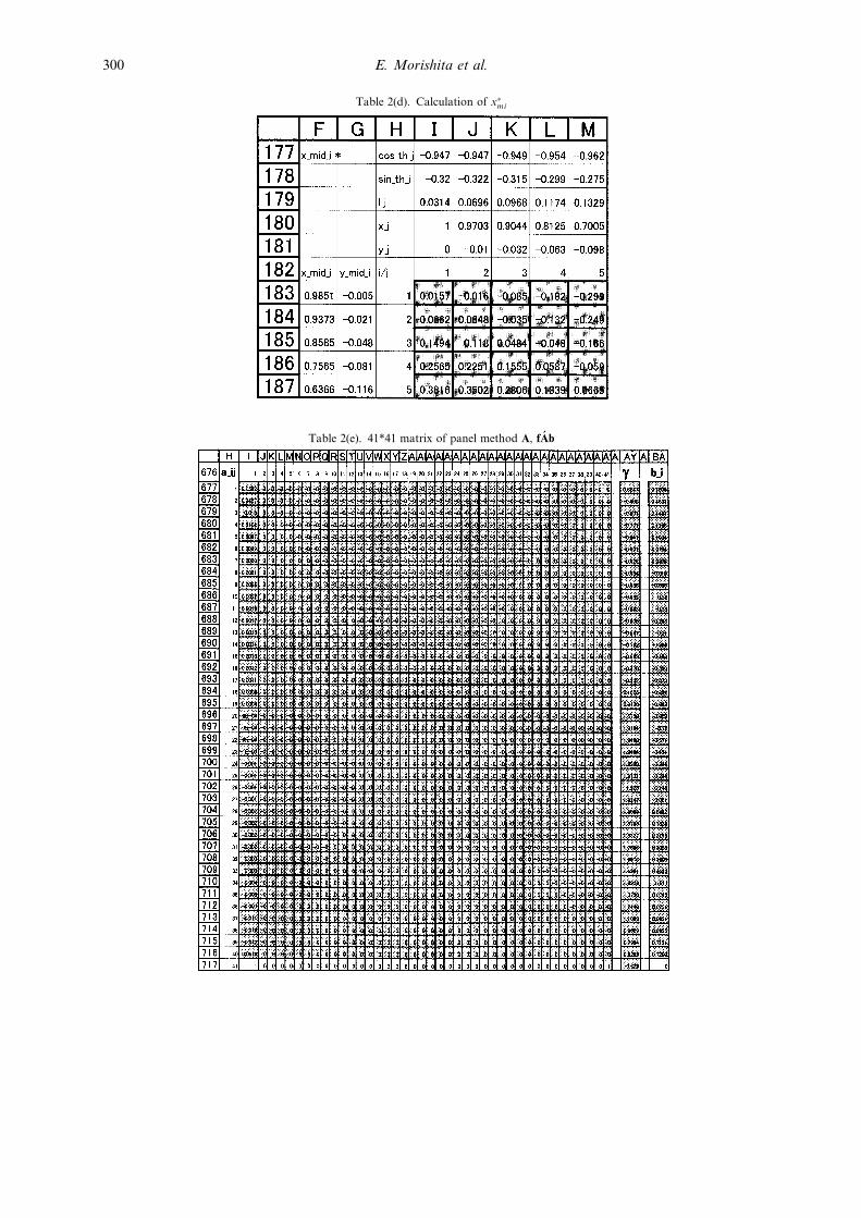
Table 2(e). 41*41 matrix of panel method A, fAÂ b

Table 2(d). Calculation of x�mi

E. Morishita et al.300

where

ai1 � Ai1; aij � Aij � Bijÿ1� j � 2; 3; . . . ;N�;aiN�1 � BiN ; bi � U1 sin��ÿ �i� �33�

Aij � C cos��i ÿ �j� �D sin��i ÿ �j�;Bij � E cos��i ÿ �j� � F sin��i ÿ �j� �34�

C � 1

2�ÿ 1ÿ x�mi

lj

� �ln

rij�1

rij� 1ÿ y�mi

lj�ij

� �� �;

D � 1

2�1ÿ x�mi

lj

� ��ij ÿ y�mi

ljln

rij�1

rij

� �;

E � 1

2�ÿ x�mi

ljln

rij�1

rijÿ 1ÿ y�mi

lj�ij

� �� �;

F � 1

2�

x�mi

lj�ij � y�mi

ljln

rij�1

rij

� ��35�

The last row of equation (32) represents the Kuttacondition at the trailing edge, i.e.

1 � N�1 � 0 �36�To solve the flow around an airfoil, it is necessaryto construct the matrix in the LHS of equation (32)in the spreadsheet. The matrix was constructedstep by step. To calculate rij in equation (25), weprepared 40� 40 cells, a section of which is shownin Table 2(c).

In cell I87 we have equation (25) as follows:

=SQRT((I$84-$F87)^2+(I$85-$G87)^2).

We copied the equation onto the rest of the cells.When we refer to row 84, we use the $ symbol [3],which is called the absolute reference, or otherwisethe alphabet and the numbers are changed auto-matically corresponding to the location of the cells(relative reference [3]). We made 40� 40 cells alsofor rij�1.

The midpoint of the panel i is obtained fromequations (23) and (24) in the local coordinate ofpanel j. The upper left 5� 5 cells out of the40� 40 cells for x�mi is shown in Table 2(d).Similar 40� 40 cells were prepared for y�mi. Wefurther proceeded to prepare several 40� 40 cellsin the same spreadsheet for ln�rij�1=rij�, �ij , C, D,E, F , Aij and Bij based on equations (25), (26),

(34) and (35). We could finally prepare equation(32) with the 41� 41 matrix based on equation(33) (Table 2(e)).

The most interesting part of this spreadsheetcalculation is the solution procedure of equation(32). Equation (32) can be expressed symbolicallyas:

A � b �37�and the solution is given by:

� Aÿ1b �38�Aÿ1 in equation (38) is expressed in this calcu-lation: =MINVERSE(I677:AW717). Then thesolution � Aÿ1b is obtained as (column AY):

=MMULT(MINVERSE(I677:AW717),BA677:BA717).

To enter MINVERSE and/or MMULT commandin the spreadsheet, we have to follow the particularkey procedure for the software we use [2] (forexample: input the equation in a cell, return key,select matrix and or vector area to input, set cursorat the end of the equation in the input area, thencontrol + shift + return).

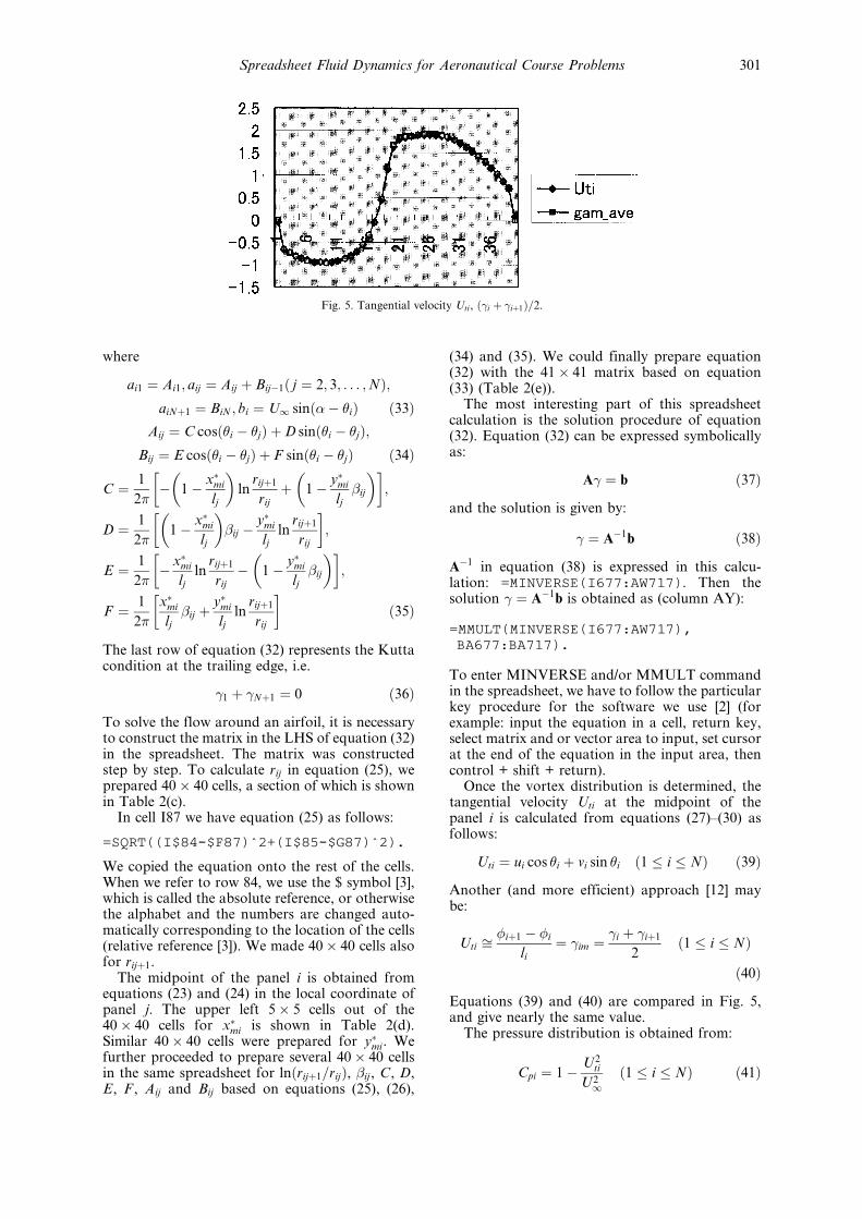
Once the vortex distribution is determined, thetangential velocity Uti at the midpoint of thepanel i is calculated from equations (27)±(30) asfollows:

Uti � ui cos �i � vi sin �i �1 � i � N� �39�Another (and more efficient) approach [12] maybe:

Uti � �i�1 ÿ �i

li� im � i � i�1

2�1 � i � N�

�40�Equations (39) and (40) are compared in Fig. 5,and give nearly the same value.

The pressure distribution is obtained from:

Cpi � 1ÿ U2ti

U21�1 � i � N� �41�

Fig. 5. Tangential velocity Uti, � i � i�1�=2.

Spreadsheet Fluid Dynamics for Aeronautical Course Problems 301

The aerodynamic characteristics are obtained fromequation (41) as follows:

Cl �XN

i�1

�ÿCxi sin�� Cyi cos�� �42�

Cd �XN

i�1

�Cxi cos�� Cyi sin�� �43�

Cm0 �XN

i�1

yi � yi�1

2cCxi ÿ xi � xi�1

2cCyi

� ��44�

xc:p:

c� ÿCm0

Cl�45�

where

Cxi � yi�1 ÿ yi

cCpi; Cyi � ÿ xi�1 ÿ xi

cCpi �46�

A simpler alternative method to calculate the liftcoefficient is:

Cl � �U1ÿ12�U21c

� 2ÿ

U1c�

2XN

i�1

i � i�1

2

� �lj

U1c�47�

Several solutions for this airfoil at different anglesof attack are shown in Fig. 6. The lift coefficientCl � 2:1 and the center of pressure 43% from thelading edge were obtained at � � 10 degrees basedon the approximate chord length c � 2. The angleof attack was changed in a cell of a spreadsheetand the solutions seen in Fig. 6 were obtained oneafter another while we were viewing the graph.(This can be done via a PC projector in the class-room and it is not surprising that students areimpressed not only by the aerodynamics but alsoby the spreadsheets.)

The validity of the panel method was checkedagainst the conformal mapping method of the

complex potential for the same airfoil (Cp_th inFig. 6). The agreement is found to be quitesatisfactory. (It has to be mentioned that theconformal mapping was also conducted on thesame spreadsheet including the complex variablecalculation.)

Care must be taken to avoid an airfoil with avery thin trailing edge which sometimes makes itdifficult to obtain accurate solutions due to theinteractions between singularities in the presentpanel method.

SFD III ± ITERATION

Partial differential equations are solved numeri-cally in discretized forms. Solutions are obtainedvia either relaxation or by a time-marching pro-cedure. These require iterations during the process.SFD Type III handles these problems, i.e. mosttypically the numerical solution of finite differenceequations [4]. The SFD technique was alsoextended to the more complicated transonicproblems [15] by using the transonic small distur-bance equation (TSDE) [12 (pp. 399±423) 16±18]:

K ÿ � � 1�M21@�

@�

� �@2�

@�2� @�

@�2� 0 �48�

where

K � 1ÿM21

�2=3; � � x

c; � � y

�;

� � c

�1=3; � � �0

U1L�49�

where K is called the transonic similarity para-meter, �0 represents the disturbance potential withdimensions. The airfoil is given by:

y�x�c� �f

x

c

� ��50�

Fig. 6. ÿCp of Karman-Trefftz airfoil: k � 1:7, z0 � �ÿ0:1; 0:1�. (a) � � 0 deg; (b) � � 5 deg; (c) � � 10 deg; (d) � � 15 deg.

E. Morishita et al.302

and the non-dimensional flow tangency conditionon the airfoil is:

@�

@�� df

d�ÿ ���� � �0� �51�

The far-field boundary condition is given by:

� � 0 �52�

The Murman-Cole method [12, 15±18] to solveequation (48) is:

�1ÿ �ij�Pij � �iÿ1jPiÿ1j �Qij � 0 �53�

where

Pij � K ÿ � � 1�M21�i�1j ÿ �iÿ1j

2��

� �� �i�1j ÿ 2�ij � �iÿ1j

��2

Qij � �ij�1 ÿ 2�ij � �ijÿ1

��2

�ij � 1 for Aij < 0 �Mij > 1�� 0 for Aij � 0 �Mij � 1�

Aij �K ÿ � � 1�M21�i�1j ÿ �iÿ1j

2���54�

Equation (53) implies that the upwind differencingis to be used at the supersonic point. The iterativesolution may be obtained from:

��n�1�ij � ��n�ij � C

�n�ij �55�

where we define:

C�n�ij � !���n�1�

ij ÿ �nij� � !���n�ij �56�

Note that ��n�1�ij in equation (56) is a temporal

value for the n� 1 iteration except for ! � 1. Wemay have from equations (54):

Pij � K ÿ � � 1�M21��n�i�1j ÿ ��n�1�

iÿ1j

2��

" #

� ��n�i�1j ÿ 2���n�ij � ���n�ij � � ��n�1�

iÿ1j

��2

�P�n�ij ÿ

2

��2A�n�ij ��

�n�ij �57�

Piÿ1j � K ÿ � � 1�M21��n�ij ÿ ��n�1�

iÿ2j

2��

" #

� ��n�ij � ���n�ij ÿ 2�

�n�1�iÿ1j � ��n�1�

iÿ2j

��2

�P�n�iÿ1j �

1

��2A�n�iÿ1j�

�n�ij �58�

Qij ���nÿ1�ij�1 � ���nÿ1�

ij�1 ÿ 2���n�ij � ���n�ij � � ��n�ijÿ1 � ���n�ijÿ1

��2

� Q�n�ij �

���nÿ1�ij�1 ÿ 2��

�n�ij � ���n�ijÿ1

��2�59�

P�n�ij , P

�n�iÿ1j , and Q

�n�ij are Pij , Piÿ1j, and Qij at �� � 0

in equations (57), (58) and (59), respectively. Theupdated values (n+1th iteration) are also usedin equations (57)±(59). Updated values areautomatically used in real calculations. Here weuse �

�n�ij in the bracket of equation (58) instead of

��n�ij � ���n�ij for simplicity and this assumption is

different from Ref. 12. Similarly:

A�n�ij �K ÿ � � 1�M2

1��n�i�1j ÿ ��n�1�

iÿ1j

2��

A�n�iÿ1j �K ÿ � � 1�M2

1��n�ij ÿ ��n�1�

iÿ2j

2���60�

P�n�ij , P

�n�iÿ1j, and Q

�n�ij are expressed using equation

(60):

P�n�ij �A

�n�ij

��n�i�1j ÿ 2�

�n�ij � ��n�1�

iÿ1j

��2�61�

P�n�ijÿ1 �A

�n�ijÿ1

��n�ij ÿ 2�

�n�iÿ1j � ��n�1�

iÿ2j

��2�62�

Q�n�ij �

��nÿ1�ij�1 ÿ 2�

�n�ij �Q

�n�ijÿ1

��2�63�

Equation (53) uses equations (57)±(59) to obtainthe following:

ÿ�1ÿ �ij� 2

����2 A�n�ij ��

�n�ij

� ���nÿ1�ij�1 ÿ 2��

�n�ij � ���n�ijÿ1

����2

��iÿ1j

A�n�iÿ1j

��2���n�ij � ÿR

�n�ij �64�

where

R�n�ij � �1ÿ �ij�P�n�ij � �iÿ1jP

�n�iÿ1j �Q

�n�ij �65�

In the present calculation, we applied the relaxa-tion factor ! for ��

�n�ij of equation (57), i.e. ��

�n�ij of

the first term in the left-hand side of equation (64).We then obtained the following expression:

C�n�ij � ÿ

1

fc=�2�C�n�ijÿ1 � C

�nÿ1�ij�1 � � R

�n�ij

ÿ2�1ÿ f Eij�A�n�ij

!��2� f Eiÿ1j

A�n�iÿ1j

��2ÿ 2

��2

�66�

Spreadsheet Fluid Dynamics for Aeronautical Course Problems 303

Equation (66) is different from the solution tech-nique in Ref. 12 (pp. 399±423). It is natural thatone may assume the positive y-direction upwardsin a spreadsheet. But the spreadsheet sweep isfrom left to right and from top to bottom,and therefore C

�n�ijÿ1 � C

�nÿ1�ij�1 in equation (66) may

become C�nÿ1�ijÿ1 � C

�n�ij�1 in the real calculation.

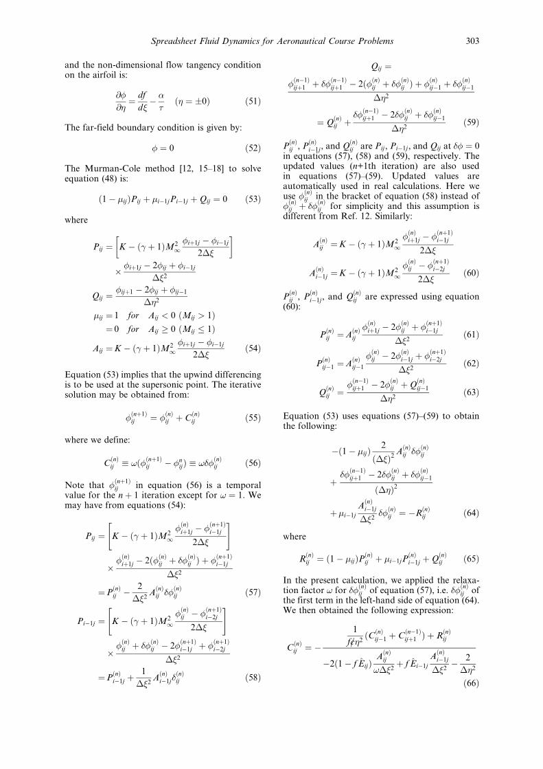
The basic computational domain is shown inFig. 7 where ÿ1 � � � 2, 0 � � � 1:25 and theairfoil locates 0 � � � 1, � � 0. 150��� � 25���cells with �� � 0:02, �� � 0:05 were used. Theboundary cells were utilized in the latter part ofthe calculation, and 152� 27 cells were usedultimately.

We are now able to start the spreadsheet calcu-lation. The conditions for the calculation were firstspecified (rows 5 and 6 in Table 3(a)).

The specific heat ratio � 1:4 and the Machnumber was 0.857. We used the iterationfunction of the spreadsheet and it is helpful inshowing the number of iterations in cell L6. This

counter can be expressed by the spreadsheetformat as: =L6+1.

This expression is called the circular reference inspreadsheet terminology [3] because cell L6requires its own value, not given at the beginning.A warning message will appear on the screen, butwe simply click the cancel button. When we startthe iteration, 0 is resumed for cell L6 and therefore1 will appear in cell L6 after one cycle.

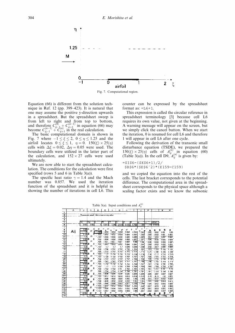
Following the derivation of the transonic smalldisturbance equation (TSDE), we prepared the150��� � 25��� cells of A

�n�ij in equation (60)

(Table 3(a)). In the cell D9, A�n�ij is given by:

=$I$6-($K$6+1)/2/$B$6*($E$6^2)*(E159-C159)

and we copied the equation into the rest of thecells. The last bracket corresponds to the potentialdifference. The computational area in the spread-sheet corresponds to the physical space although ascaling factor exists and we know the subsonic

Fig. 7. Computational region.

Table 3(a). Input conditions and A�n�ij

E. Morishita et al.304

�A�n�ij > 0� and/or the supersonic region �A�n�ij < 0�from the spreadsheet (see Table 3(a)).

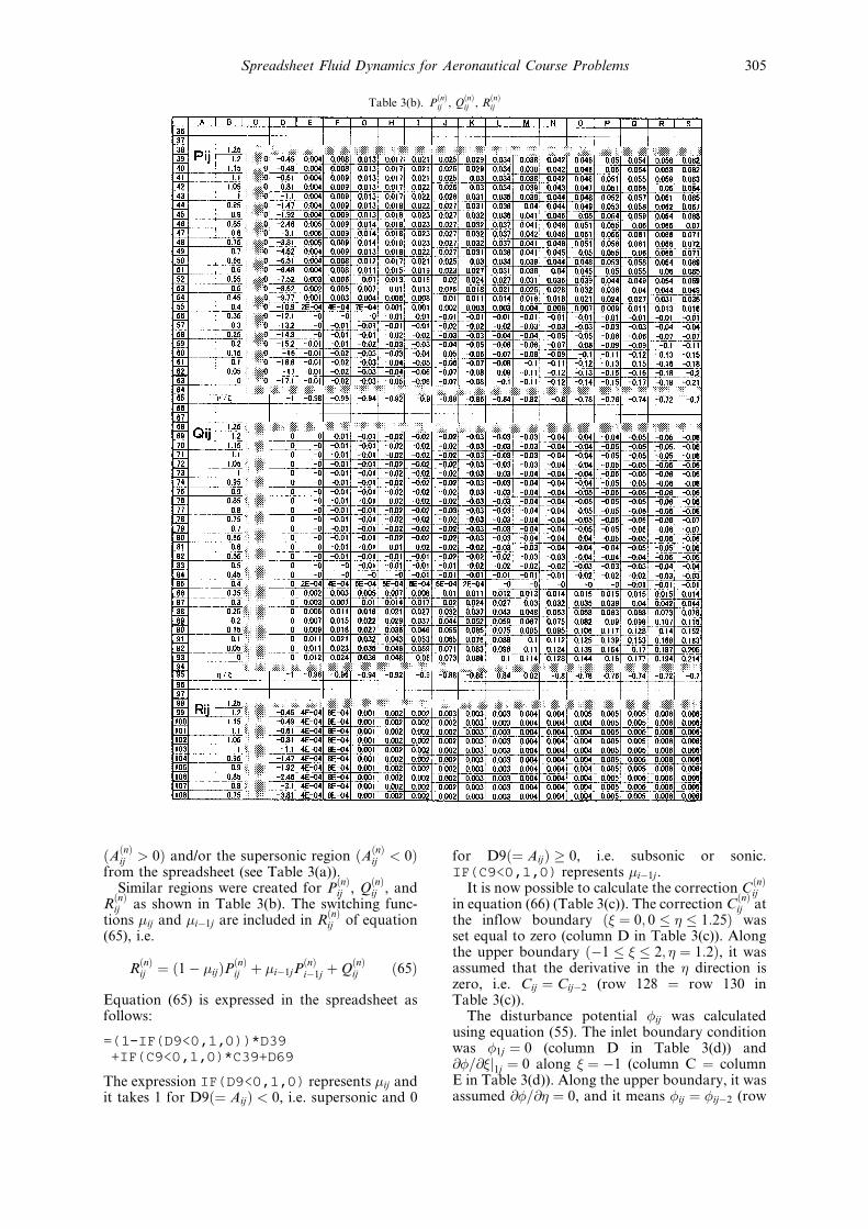
Similar regions were created for P�n�ij , Q

�n�ij , and

R�n�ij as shown in Table 3(b). The switching func-

tions �ij and �iÿ1j are included in R�n�ij of equation

(65), i.e.

R�n�ij � �1ÿ �ij�P�n�ij � �iÿ1jP

�n�iÿ1j �Q

�n�ij �65�

Equation (65) is expressed in the spreadsheet asfollows:

=(1-IF(D9<0,1,0))*D39+IF(C9<0,1,0)*C39+D69

The expression IF(D9<0,1,0) represents �ij andit takes 1 for D9�� Aij� < 0, i.e. supersonic and 0

for D9�� Aij� � 0, i.e. subsonic or sonic.IF(C9<0,1,0) represents �iÿ1j.

It is now possible to calculate the correction C�n�ij

in equation (66) (Table 3(c)). The correction C�n�ij at

the inflow boundary �� � 0; 0 � � � 1:25� wasset equal to zero (column D in Table 3(c)). Alongthe upper boundary �ÿ1 � � � 2; � � 1:2�, it wasassumed that the derivative in the � direction iszero, i.e. Cij � Cijÿ2 (row 128 � row 130 inTable 3(c)).

The disturbance potential �ij was calculatedusing equation (55). The inlet boundary conditionwas �1j � 0 (column D in Table 3(d)) and@�=@�j1j � 0 along � � ÿ1 (column C � columnE in Table 3(d)). Along the upper boundary, it wasassumed @�=@� � 0, and it means �ij � �ijÿ2 (row

Table 3(b). P�n�ij , Q

�n�ij , R

�n�ij

Spreadsheet Fluid Dynamics for Aeronautical Course Problems 305

158 � row 160 in Table 3(d)). The symmetricboundary condition was applied along the �-axis�� � 0� and this means that row 184 � row 182 inTable 3(d) except on the airfoil surface�0 � � � 1�.

The leading edge is cell BB183 and the airfoil isin row 183 in Table 3(e). The boundary conditionequation (51) on the airfoil at � � 0 is given by:

�i2 ÿ �i0

2��� df

d��0 � � � 1� �67�

We used a parabolic airfoil in Fig. 8:

y

c� �f

x

c

� �� �2

x

c1ÿ x

c

� ��68�

We obtain the following from equation (68):

df

d�� 2ÿ 4� �69�

From equation (67), the boundary conditionbecomes:

�i0 � �i2 ÿ 2��df

d��70�

Equation (70) for the cell BE184 in Table 3(e) isgiven by:

=BE182-2*$C$6*BE$189.

Table 3(d). Inlet �ij

Table 3(c). C�n�ij

E. Morishita et al.306

The outlet condition is given by:

d�

d�� 0 �71�

In the finite difference form, equation (71) is givenby:

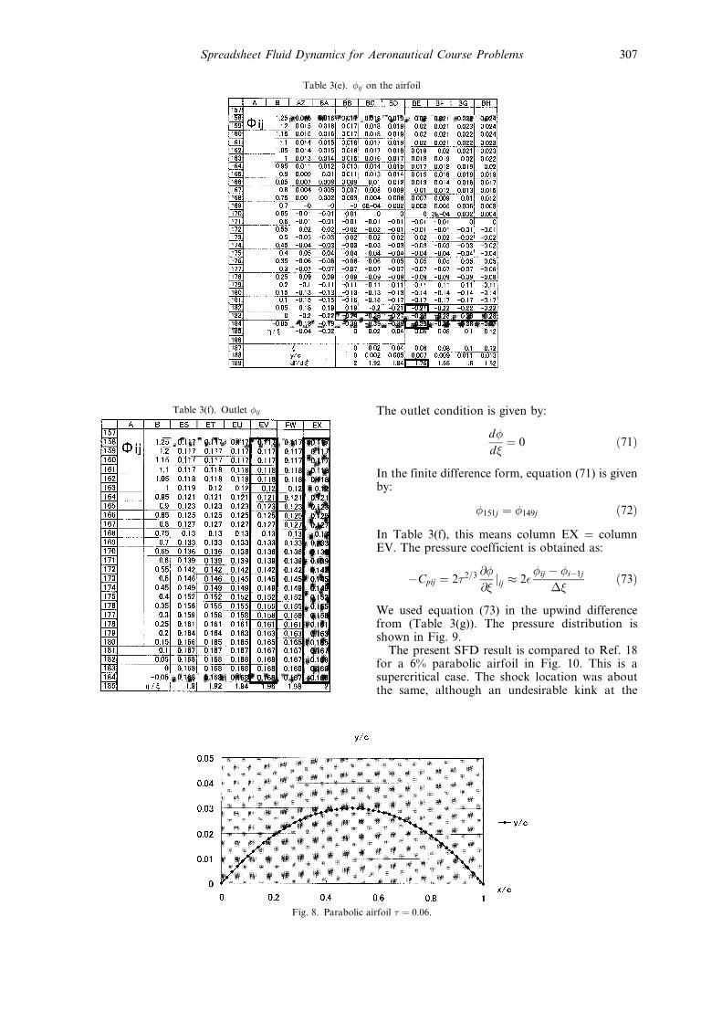
�151j � �149j �72�In Table 3(f), this means column EX � columnEV. The pressure coefficient is obtained as:

ÿCpij � 2�2=3 @�

@�jij � 2�

�ij ÿ �iÿ1j

���73�

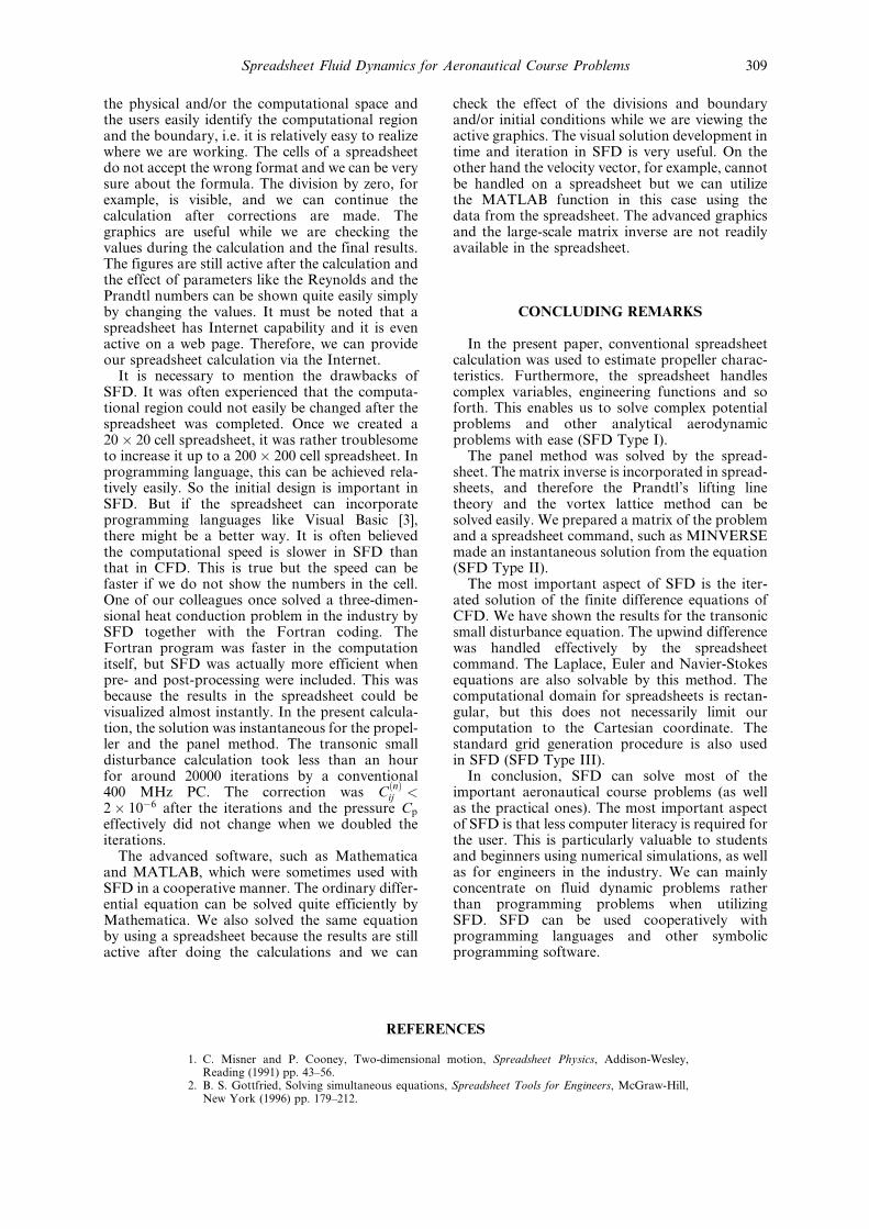
We used equation (73) in the upwind differencefrom (Table 3(g)). The pressure distribution isshown in Fig. 9.

The present SFD result is compared to Ref. 18for a 6% parabolic airfoil in Fig. 10. This is asupercritical case. The shock location was aboutthe same, although an undesirable kink at the

Table 3(f). Outlet �ij

Table 3(e). �ij on the airfoil

Fig. 8. Parabolic airfoil � � 0:06.

Spreadsheet Fluid Dynamics for Aeronautical Course Problems 307

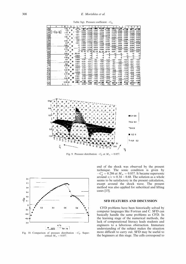
end of the shock was observed by the presenttechnique. The sonic condition is given byÿC�p � 0:286 at M1 � 0:857. It became supersonicaround x=c � 0:34ÿ 0:68. The solution as a wholeseems to be satisfactory in the present calculation,except around the shock wave. The presentmethod was also applied for subcritical and liftingcases [15].

SFD FEATURES AND DISCUSSION

CFD problems have been historically solved bycomputer languages like Fortran and C. SFD canbasically handle the same problems as CFD. Inthe learning stage of the numerical methods, thelack of computational literacy leads students andengineers to a laborious obstruction. Immatureunderstanding of the subject makes the situationmore difficult to carry out. SFD may be useful tothe beginners at this stage. The cells correspond to

Fig. 9. Pressure distribution ÿCp at M1 � 0:857.

Table 3(g). Pressure coefficient ÿCpij

Fig. 10. Comparison of pressure distribution ÿCp. Super-critical M1 � 0:857.

E. Morishita et al.308

the physical and/or the computational space andthe users easily identify the computational regionand the boundary, i.e. it is relatively easy to realizewhere we are working. The cells of a spreadsheetdo not accept the wrong format and we can be verysure about the formula. The division by zero, forexample, is visible, and we can continue thecalculation after corrections are made. Thegraphics are useful while we are checking thevalues during the calculation and the final results.The figures are still active after the calculation andthe effect of parameters like the Reynolds and thePrandtl numbers can be shown quite easily simplyby changing the values. It must be noted that aspreadsheet has Internet capability and it is evenactive on a web page. Therefore, we can provideour spreadsheet calculation via the Internet.

It is necessary to mention the drawbacks ofSFD. It was often experienced that the computa-tional region could not easily be changed after thespreadsheet was completed. Once we created a20� 20 cell spreadsheet, it was rather troublesometo increase it up to a 200� 200 cell spreadsheet. Inprogramming language, this can be achieved rela-tively easily. So the initial design is important inSFD. But if the spreadsheet can incorporateprogramming languages like Visual Basic [3],there might be a better way. It is often believedthe computational speed is slower in SFD thanthat in CFD. This is true but the speed can befaster if we do not show the numbers in the cell.One of our colleagues once solved a three-dimen-sional heat conduction problem in the industry bySFD together with the Fortran coding. TheFortran program was faster in the computationitself, but SFD was actually more efficient whenpre- and post-processing were included. This wasbecause the results in the spreadsheet could bevisualized almost instantly. In the present calcula-tion, the solution was instantaneous for the propel-ler and the panel method. The transonic smalldisturbance calculation took less than an hourfor around 20000 iterations by a conventional400 MHz PC. The correction was C

�n�ij <

2� 10ÿ6 after the iterations and the pressure Cp

effectively did not change when we doubled theiterations.

The advanced software, such as Mathematicaand MATLAB, which were sometimes used withSFD in a cooperative manner. The ordinary differ-ential equation can be solved quite efficiently byMathematica. We also solved the same equationby using a spreadsheet because the results are stillactive after doing the calculations and we can

check the effect of the divisions and boundaryand/or initial conditions while we are viewing theactive graphics. The visual solution development intime and iteration in SFD is very useful. On theother hand the velocity vector, for example, cannotbe handled on a spreadsheet but we can utilizethe MATLAB function in this case using thedata from the spreadsheet. The advanced graphicsand the large-scale matrix inverse are not readilyavailable in the spreadsheet.

CONCLUDING REMARKS

In the present paper, conventional spreadsheetcalculation was used to estimate propeller charac-teristics. Furthermore, the spreadsheet handlescomplex variables, engineering functions and soforth. This enables us to solve complex potentialproblems and other analytical aerodynamicproblems with ease (SFD Type I).

The panel method was solved by the spread-sheet. The matrix inverse is incorporated in spread-sheets, and therefore the Prandtl's lifting linetheory and the vortex lattice method can besolved easily. We prepared a matrix of the problemand a spreadsheet command, such as MINVERSEmade an instantaneous solution from the equation(SFD Type II).

The most important aspect of SFD is the iter-ated solution of the finite difference equations ofCFD. We have shown the results for the transonicsmall disturbance equation. The upwind differencewas handled effectively by the spreadsheetcommand. The Laplace, Euler and Navier-Stokesequations are also solvable by this method. Thecomputational domain for spreadsheets is rectan-gular, but this does not necessarily limit ourcomputation to the Cartesian coordinate. Thestandard grid generation procedure is also usedin SFD (SFD Type III).

In conclusion, SFD can solve most of theimportant aeronautical course problems (as wellas the practical ones). The most important aspectof SFD is that less computer literacy is required forthe user. This is particularly valuable to studentsand beginners using numerical simulations, as wellas for engineers in the industry. We can mainlyconcentrate on fluid dynamic problems ratherthan programming problems when utilizingSFD. SFD can be used cooperatively withprogramming languages and other symbolicprogramming software.

REFERENCES

1. C. Misner and P. Cooney, Two-dimensional motion, Spreadsheet Physics, Addison-Wesley,Reading (1991) pp. 43±56.

2. B. S. Gottfried, Solving simultaneous equations, Spreadsheet Tools for Engineers, McGraw-Hill,New York (1996) pp. 179±212.

Spreadsheet Fluid Dynamics for Aeronautical Course Problems 309

3. J. Walkenbach, Creating and using formulas, Excel 97 Bible, IDG Books Worldwide, Foster City(1996).

4. E. Morishita, Spreadsheet fluid dynamics, J. Aircraft, 36, 41 (1999) pp. 720±723.5. D. O. Dommasch, S. S. Sherby and T. F. Conolly, Vortex theory, Airplane Aerodynamics, Pitman,

New York, 9 (1951) pp. 184±195.6. A. Fage, C. N. H. Lock, R. G. Howard and H. Bateman, Experiments with a family of

airscrews including the effect of tractor and pusher bodies, Reports and Memoranda, No. 829(1922) p. 61.

7. I. Imai, A circular cylinder in arbitrary motion, Fluid Dynamics (in Japanese), Iwanami, Tokyo(1970) pp. 73±78.

8. S. Schreier, The Howarth Transformation, Compressible Flow, John Wiley & Sons, New York(1982) pp. 309±315.

9. E. R. van Driest, Turbulent boundary layer in compressible fluids, J. Aeronautical Sciences, 18, 3(1951) pp. 145±160.

10. F. W. Matting, D. R. Chapman, J. R. Nyholm and A. G. Thomas, Turbulent skin friction at highmach numbers and Reynolds numbers in air and helium, NASA TR R-82 (1961) pp. 28±29.

11. A. Mizuno, Karman-Trefftz, wing section, An Introduction to CFD (in Japanese), Asakura, Tokyo(1990) pp. 80±96.

12. J. Moran, Nonelliptic Lift distributions, An Introduction to Theoretical and ComputationalAerodynamics, John Wiley & Sons, New York (1984) pp. 124±153.

13. T. Moriya, Theory of Propeller, An Introduction to Aerodynamics (in Japanese), Baifukan, Tokyo(1970) pp. 177±200.

14. K. Yuki, Performance prediction of a two-blade propeller by vortex lattice method (in Japanese),graduation thesis, Department of Aeronautics and Astronautics, University of Tokyo (1999).

15. Y. Iwata, Flow around a two-dimensional airfoil solved by transonic small disturbance equation(in Japanese), graduation thesis, Department of Aeronautics and Astronautics, University ofTokyo (1999).

16. E. M. Murman, Analysis of embedded shock waves calculated by relaxation methods, AIAAJournal, 12, 6 (1974) pp. 626±633.

17. E. D. Knechtel, Experimental investigation at transonic speeds of pressure distribution overwedge and circular arc sections and evaluation of perforated wall interference, NASA TN D15(1959).

18. D. J. Collins and J. A. Krupp, Experimental and theoretical investigations in two-dimensionaltransonic flow, AIAA Journal, 12, 6 (1974) pp. 771±778.

19. H. Yoshida, Flow around a cavity solved by small disturbance and Euler equations (inJapanese), graduation thesis, Department of Aeronautics and Astronatics, University of Tokyo(1999).

20. K. Fujii, TVD scheme, Numerical Methods for Computational Fluid Dynamics (in Japanese),University of Tokyo Press (1994) pp. 68±76.

21. K. A. Hoffmann and S. T. Chiang, MacCormack explicit formulation, Computational FluidDynamics for Engineers, II, Engineering Education System, Wichita (1993) pp. 205±207.

22. C. Y. Chow, Propagation of a finite-amplitude wave: formation of a shock, An Introduction toComputational Fluid Mechanics, John Wiley & Sons, New York (1979) pp. 203±214.

23. J. D. Anderson, Jr., Determination of the compatibility equations, Modern Compressible Flow withHistorical Perspective, McGraw-Hill, New York (1982) pp. 260±305.

24. A. H. Shapiro, Sharp-corner nozzle, The Dynamics and Thermodynamics of Compressible FluidFlow, Vol. I, Ronald Press, New York (1953) pp. 512±516.

25. J. T. Stuart, On the non-linear mechanics of hydrodynamic stability, J. Fluid Mechanics, 4 (1958)p. 15.

26. Schlichting, Flow between concentric rotating cylinders, H, Boundary-Layer Theory, McGraw-Hill, New York (1979) pp. 525±529.

27. J. E. Burkhalter and E. L. Koschmieder, Steady supercritical taylor vortices after sudden starts,The Physics of Fluids, 17, 11 (1974) pp. 1929±1935.

28. M. van Dyke, 127, Axisymmetric laminar Taylor vortices, An Album of Fluid Motion, ParabolicPress, Stanford, 1982, pp. 76±77.

29. G. I. Taylor, Fluid friction between rotating cylinders I-torque measurements, Proc. Royal Soc.London, Series A, 157, 1936 pp. 546±564.

Etsuo Morishita, Professor, Department of Aeronautics and Astronautics, Graduate Schoolof Engineering, University of Tokyo. Japan, B.Eng. (1972), M. Eng. (1974), Dr.Eng. (1985),University of Tokyo, M.Sc. (1982), University of Cambridge, 1974±1987: MitsubishiElectric Corporation, 1987±Present: University of Tokyo, Associate Professor (1987±1993), Professor (1993±). Achievements include scroll compressor and co-rotating scrollvacuum pump development at MELCO. Contributor to technical journals and interna-tional patents holder. Presently engaged in the education and the research of aerodynamicsat the University of Tokyo. Name appeared in Who's Who in Science and Engineering1994/1995(USA)

Yohei Iwata, graduate student (Master course 2nd year), Department of Aeronautics andAstronautics, Graduate School of Engineering, University of Tokyo. His current subjectis `Spreadsheet Fluid Dynamics of Unsteady Flows'. He solved the transonic smalldisturbance equation by SFD.

E. Morishita et al.310

Kentaro Yuki, Presently Japanese Patent Office. Former graduate student (Master course),Department of Aeronautics and Astronautics, Graduate School of Engineering, Universityof Tokyo. He solved the propeller VLM by SFD.

Haruhiko Yoshida, graduate student (Master course 2nd year), Department of Aeronauticsand Astronautics, Graduate School of Engineering, University of Tokyo. His currentsubject is `A New Scheme for High-Speed Flows Based on the Time-Space Conservation'.He solved the Euler equation by SFD.

Spreadsheet Fluid Dynamics for Aeronautical Course Problems 311