SPONTANEOUS FOUR-WAVE MIXING

IN STANDARD BIREFRINGENT FIBER

by

Jamy B. Moreno

A thesis submitted to the Faculty of the University of Delaware in partialfulfillment of the requirements for the degree of Master of Science in Physics andAstronomy

Spring 2012

c© 2012 Jamy B. MorenoAll Rights Reserved

SPONTANEOUS FOUR-WAVE MIXING

IN STANDARD BIREFRINGENT FIBER

by

Jamy B. Moreno

Approved:Virginia Lorenz, Ph.D.Professor in charge of thesis on behalf of the Advisory Committee

Approved:George Hadjipanayas, Ph.D.Chair of the Department of Physics and Astronomy

Approved:George H. Watson, Ph.D.Dean of the College of Arts and Sciences

Approved:Charles G. Riordan, Ph.D.Vice Provost for Graduate and Professional Education

ACKNOWLEDGMENTS

First and foremost I would like to thank my advisor, Professor Virginia Lorenz,

who has guided and supported me throughout my whole graduate career. She has been

a source of inspiration and has always believed in me, and for that I thank her.

I would like to give my most sincerest thanks to Offir Cohen who has worked

closely with me from when I started up until I finished. Thank you for your patience

and your knowledge. I have learned so much from you.

I would like to also extend my thanks to my committee members Professor

Matthew DeCamp and Professor Jamie Holder for their guidance.

I would like thank the members of the Ultrafast group Seth Meiselman, Bin

Fang, and Halise Celik. Not only did they provide useful discussions and insight, but

they also made for a wonderful and fun group to work with.

To all the friends I have made here at the University of Delaware, thank you

for making my graduate experience a wonderful one. Particular thanks goes to Kevin

Haughey. Thanks for everything. I would also like to give my thanks to my officemates,

my best friends here, the “chicas”: Katie Mulrey, Inci Ruzybayev, and Han Zou. The

past few years would definitely not have been nearly as fun without you.

Lastly, I would like to thank my family. Thank you for being so understanding

and supportive through everything. I could not have done it without you.

iii

TABLE OF CONTENTS

LIST OF FIGURES . . . . . . . . . . . . . . . . . . . . . . . . . . . . . . . viABSTRACT . . . . . . . . . . . . . . . . . . . . . . . . . . . . . . . . . . . vii

Chapter

1 INTRODUCTION . . . . . . . . . . . . . . . . . . . . . . . . . . . . . . 1

1.1 Linear-Optics Quantum-Computation . . . . . . . . . . . . . . . . . . 11.2 Hong-Ou-Mandel (HOM) Interference . . . . . . . . . . . . . . . . . . 21.3 Single Photon Generators . . . . . . . . . . . . . . . . . . . . . . . . 3

1.3.1 Single-Emitter Photon Sources . . . . . . . . . . . . . . . . . . 41.3.2 Heralded Photons . . . . . . . . . . . . . . . . . . . . . . . . . 4

1.4 Standard Fibers . . . . . . . . . . . . . . . . . . . . . . . . . . . . . . 61.5 Phasematching and Energy Conservation in SFWM . . . . . . . . . . 71.6 Outline . . . . . . . . . . . . . . . . . . . . . . . . . . . . . . . . . . . 8

2 SPONTANEOUS FOUR-WAVE MIXING USING DEGENERATEPUMP PHOTONS: EXPERIMENTAL IMPLEMENTATION . . 9

2.1 Birefringent Standard Fibers . . . . . . . . . . . . . . . . . . . . . . . 92.2 Phasematching for Degenerate Pump Photons . . . . . . . . . . . . . 102.3 Experimental Setup . . . . . . . . . . . . . . . . . . . . . . . . . . . . 11

2.3.1 Second-Order Coherence Function . . . . . . . . . . . . . . . . 142.3.2 Heralding Efficiency . . . . . . . . . . . . . . . . . . . . . . . 15

3 SPONTANEOUS FOUR-WAVE MIXING USINGNON-DEGENERATE PUMP PHOTONS: A THEORETICALSTUDY . . . . . . . . . . . . . . . . . . . . . . . . . . . . . . . . . . . . 17

3.1 Phasematching for Non-Degenerate Pump Photons . . . . . . . . . . 17

iv

3.2 Joint Spectral Amplitude . . . . . . . . . . . . . . . . . . . . . . . . . 193.3 Interaction in the Fiber . . . . . . . . . . . . . . . . . . . . . . . . . . 22

3.3.1 Regime 1: negligible temporal walk-off between the two pumpbeams (|στp| << 1) . . . . . . . . . . . . . . . . . . . . . . . . 24

3.3.2 Regime 2: |στp| >> 1 . . . . . . . . . . . . . . . . . . . . . . . 24

3.4 Purity and Factorability . . . . . . . . . . . . . . . . . . . . . . . . . 263.5 Numerical Methods . . . . . . . . . . . . . . . . . . . . . . . . . . . . 28

4 SUMMARY . . . . . . . . . . . . . . . . . . . . . . . . . . . . . . . . . . 31

4.1 Conclusion . . . . . . . . . . . . . . . . . . . . . . . . . . . . . . . . . 31

BIBLIOGRAPHY . . . . . . . . . . . . . . . . . . . . . . . . . . . . . . . . 33

Appendix

A JOINT SPECTRAL AMPLITUDE CALCULATION . . . . . . . . 35

A.1 Regime 1 calculation . . . . . . . . . . . . . . . . . . . . . . . . . . . 41A.2 Regime 2 calculation . . . . . . . . . . . . . . . . . . . . . . . . . . . 42

v

LIST OF FIGURES

1.1 Hong-Ou-Mandel Interference . . . . . . . . . . . . . . . . . . . . . 3

1.2 Heralded Photons . . . . . . . . . . . . . . . . . . . . . . . . . . . . 5

1.3 Step-Index Model for Standard Fibers . . . . . . . . . . . . . . . . 7

2.1 Phasematching plot for degenerate pump photons . . . . . . . . . . 12

2.2 Experimental setup of SFWM process using degenerate pump photons 13

2.3 Normalized spectra using Fibercore 800G . . . . . . . . . . . . . . . 14

3.1 Phasematching plot for nondegenerate pump photons . . . . . . . . 18

3.2 Energy conservation, phasematching, and joint spectrum for ∆λ =45nm . . . . . . . . . . . . . . . . . . . . . . . . . . . . . . . . . . . . 23

3.3 Calculated Joint spectral amplitude in the regime when στp, στ << 1 25

3.4 Joint spectral amplitude in the regime when |στp|, |στ | >> 1 . . . 26

3.5 Joint spectral probability for detunings ∆λ = 50 nm, 150 nm, and240 nm with central wavelength λp = 700 nm . . . . . . . . . . . . 29

3.6 Purity and min|fp1 − fs|, |fp1 − fi| as a function of detuning, ∆λ, inthe regime where |στp| >> 1. τ = −1

2τp . . . . . . . . . . . . . . . . 30

vi

ABSTRACT

This thesis presents an experimental implementation and a theoretical inves-

tigation of a source of photon-pairs. The source is based on the nonlinear optical

interaction of two strong pump pulses in a birefringent single-mode optical fiber. The

interaction is mediated by the χ(3) susceptibility of the fiber medium and results in the

spontaneous creation of two photons, referred to as the signal and idler. Because the

signal and idler photons are produced simultaneously, one of the photons can be used

to herald the other. The creation of photons in such a fiber is motivated by the fact

that their mode is matched for coupling into quantum information networks that are

composed of similar fibers. Indeed, such a photon-pair source has already been shown

to be capable of producing photon-pairs that are suitable for quantum computing and

quantum communication applications.

In this thesis we experimentally confirm that photon pairs can be generated

through this type of fiber, using degenerate pump pulses. We then investigate theoret-

ically the spectral correlations introduced between the photons when they are created

by two pump pulses with different wavelengths. We find that the group velocity differ-

ence between the two pumps can be utilized to switch the nonlinear optical interaction

on and off gradually, and showed that this feature can be employed for the creation

of 100% uncorrelated photon pairs, which is a necessary condition for the heralding of

pure single photons.

vii

Chapter 1

INTRODUCTION

1.1 Linear-Optics Quantum-Computation

With the advancement of information technology, systems are becoming smaller,

thus requiring a quantum mechanical description. In 1985, David Deutsch laid the

foundations for the field of quantum computation [1], by proposing logic gates operating

on quantum systems. Quantum computation exploits the superposition principle and

non-classical correlations of quantum mechanics.

While a classical computer uses bits that take values of either zero or one to

store information, a quantum computer utilizes qubits. A qubit can represent a zero, a

one, or any superposition of these states. In general, a quantum computer that has n

qubits can be in a superposition of up to 2n different states simultaneously, compared

to a classical computer that can only be in one of the 2n states at a time. Because of

this fact, it is believed that quantum computers are able to solve problems much faster

than classical computers.

Shor’s algorithm [2] is a quantum algorithm that finds the prime factors of an

integer N . When implemented, this algorithm takes a time that goes as a polyno-

mial of N , a much faster time than that of a classical computer whose computation

time is ∼ exp(N13 ). Because of this, Shor’s algorithm, when employed on a quantum

computer with a sufficient number of qubits, can be used to break public-key cryptog-

raphy schemes including the commonly used RSA scheme, illustrating one of the many

applications of quantum computation.

As stated above, a qubit is the quantum counterpart to a classical bit. It is the

basic unit of quantum computation. One good candidate for implementing a qubit is

1

the photon since it rarely interacts with its environment and is ideal for information

transfer over large distances [3]. It was believed that to obtain scalable quantum

information processing, nonlinear couplings between optical modes was necessary, until

2001 when Knill, Laflamme, and Milburn (KLM) proposed a scheme for quantum

computation using linear optics [4].

In order to implement the so-called linear optics quantum computation (LOQC)

scheme, three nontrivial resources have to be available: quantum memories, photon

counting detectors, and single photon generators. Research has been conducted and

produced viable methods for the first resource, namely, state storage and retrieval [5].

Photon counting detectors have also been studied and research in this area has provided

methods for photon-number resolving detection [6].

The third nontrivial resource, a single photon generator, needs to be a source

that produces the same photon each and every time in order to use it for the LOQC

scheme. Identical and indistinguishable photons will undergo Hong-Ou-Mandel (HOM)

interference, which is described in the next section. This thesis presents a method to

realize such a source.

1.2 Hong-Ou-Mandel (HOM) Interference

The Hong-Ou-Mandel (HOM) interference is a two-photon interference that

takes place when two identical and indistinguishable photons interfere on a 50% beam

splitter, as shown in figure 1.1.

Assume we have two photons that are identical in every degree of freedom such

that they have the same polarization and spectral-temporal shape, and are also in a

pure wave-packet. In a lossless beamsplitter, a photon that is reflected picks up a π/2

phase relative to the transmitted photon [8]. Therefore, the situation when the two

identical photons are reflected destructively interferes with the situation when both

photons are transmitted, as shown in the top picture in figure 1.1. Thus, the two

photons bunch together in the same arm, yielding a superposition of both photons

being in either arm, as depicted in the lower picture of figure 1.1.

2

Figure 1.1: Two identical photons interfering on a 50% lossless beamsplitter. Thecase when both photons are reflected destructively interferes with the sit-uation when they are both transmitted (top). The resulting two-photonstate is then a superposition of both photons bunching together and leav-ing the beamsplitter at the same arm (bottom).

For photon sources to be applied to an LOQC scheme, they have to produce

photons that interfere in such a fashion, i.e. that are pure and identical.

1.3 Single Photon Generators

An ideal single photon source emits a single photon in each triggering event. This

is different than a “classical” source such as an attenuated laser, where the number

of photons in each pulse follows a Poissonian distribution, and hence does not contain

necessarily one and only one photon.

To date, there are two main techniques to generate single photons. The first

technique uses a single emitting system that produces photons via spontaneous emis-

sion. The second technique randomly produces photons, although always in pairs.

The pair is created simultaneously; therefore, the detection of one photon implies the

presence of the other. Such a photon is considered a heralded photon.

3

1.3.1 Single-Emitter Photon Sources

An example of a single-emitter photon source that has already been implemented

is an atom trapped in a cavity via a dipole trap. A single photon can be generated on-

demand by applying a laser pulse to the trapped atom. The cavity is comprised of two

highly reflective mirrors and its purpose is to ensure that all photons generated are sent

in the same spatial mode. This method produces single photons whose energy varies

very little [9]. However, the experimental setup is highly complicated and requires

several laser beams and stabilized cavities.

Instead of using a cavity, a molecule may be used and trapped inside a matrix to

form an on-demand single photon source. However, since molecules have many vibra-

tional levels available, the trapped molecule must be kept under cryogenic conditions

[10, 11] so as to suppress these vibrational levels. This again poses an inconvenience

because of its complexity.

Quantum dots may also serve as a viable single photon emitter. Similar to

trapped molecules, the quantum dots must be kept under cryogenic conditions. The

produced photons vary in energy and are distinguishable, making them unusable for

the LOQC scheme.

The examples of single emitters stated above are indeed realizable on-demand

single-emitter photon sources, however, they suffer from either the complex nature of

the experimental setup, and/or the distinguishability of the generated photons.

1.3.2 Heralded Photons

The technique of heralded photon generation described in this section randomly

produces photons, but always in pairs. Therefore, the presence of one heralds the

other. The experimental implementation of heralded photons is simple compared to the

single-photon emitters described in the previous section and therefore have been widely

used. There are two common methods to produce heralded photons; the first is called

spontaneous parametric down conversion (SPDC), the other is called spontaneous four-

wave mixing (SFWM).

4

SPDC is a three-wave mixing process in which a single pump photon produces a

photon-pair via a nonlinear process that is mediated by a χ(2) nonlinear susceptibility.

Materials whose leading non-linear susceptibility term is the χ(2) term include bulk

crystals such as beta-barium borate (BBO). An external electromagnetic field, the

pump, is annihilated by the medium, then produces two daughter photons [12]. Both

daughter photons are created simultaneously, and therefore, one heralds the other.

This technique of heralding has been applied to another process, namely, spon-

taneous four-wave mixing (SFWM), which is the process we focus on in this thesis.

In this case, the process is mediated by a χ(3) nonlinear susceptibility, wherein two

pump photons (as opposed to only one in the case of SPDC) that are not necessarily

degenerate are annihilated by the medium, and then produce two different photons,

called the signal and idler. In amorphous materials like glass, the leading nonlinear

susceptibility term is the χ(3) term.

Figure 1.2: Schematic and energy-level diagram for SPDC (top). For this process, asingle pump photon is annihilated in a medium with a χ(2) susceptibilityand produces two daughter photons. The bottom illustrates a SFWM(bottom) interaction and corresponding energy-level diagram. A SFWMprocess is mediated by a χ(3) susceptibility. Two (not necessarily) degen-erate pump photons are annihilated in the medium and then produce asignal and idler photon.

Figure 1.2 illustrate a schematic of an SPDC and SFWM process. In both cases,

5

energy must be conserved (see level diagram). For the case of SPDC, the frequency of

the pump photon must be equal to the sum of frequencies of the daughter photons. In

SFWM, the frequency of two pump photons (not necessarily degenerate) must sum up

to the frequencies of the generated photon pair.

It should be noted that a SFWM process has the flexibility to use any two pump

photons and generate signal and idler photons (that satisfy both energy and momentum

conservation), unlike the SPDC process that is limited to just a single pump. Because

of this, we have chosen to further investigate SFWM, specifically in standard optical

fibers.

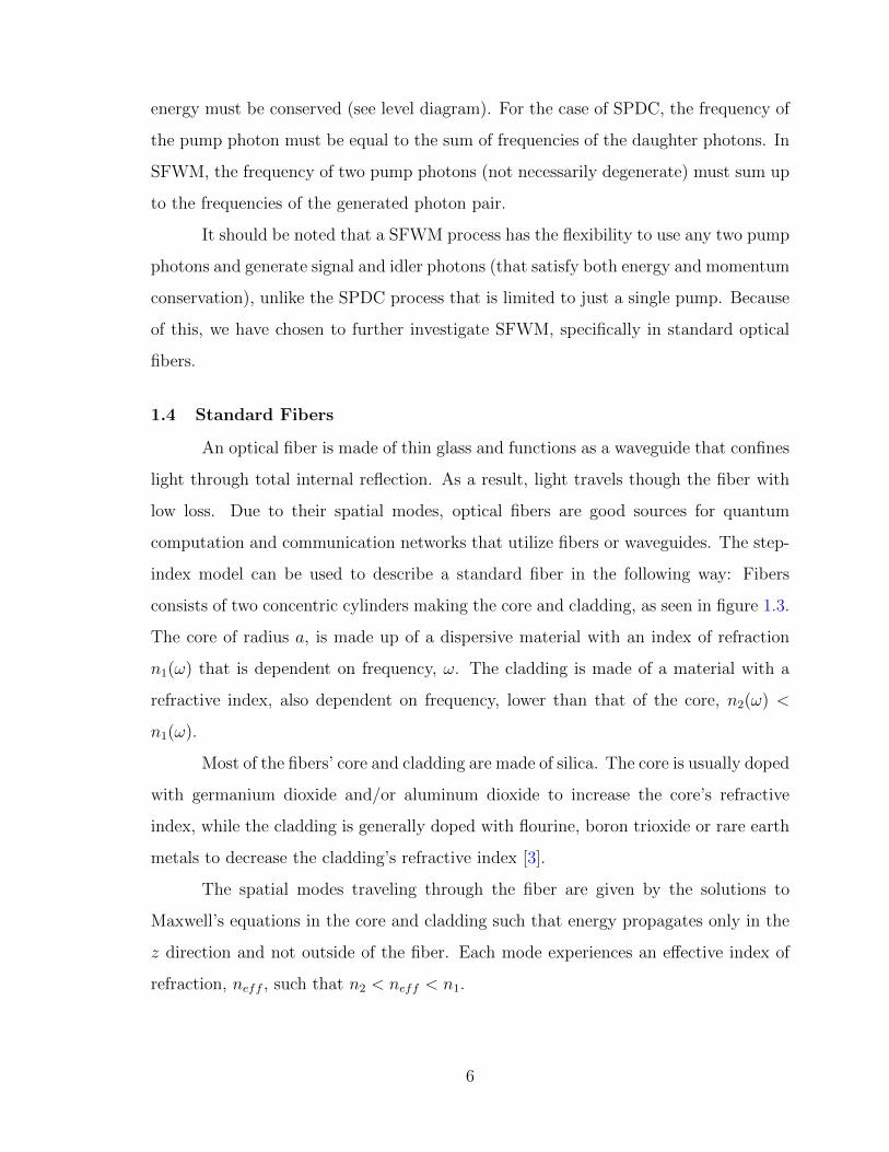
1.4 Standard Fibers

An optical fiber is made of thin glass and functions as a waveguide that confines

light through total internal reflection. As a result, light travels though the fiber with

low loss. Due to their spatial modes, optical fibers are good sources for quantum

computation and communication networks that utilize fibers or waveguides. The step-

index model can be used to describe a standard fiber in the following way: Fibers

consists of two concentric cylinders making the core and cladding, as seen in figure 1.3.

The core of radius a, is made up of a dispersive material with an index of refraction

n1(ω) that is dependent on frequency, ω. The cladding is made of a material with a

refractive index, also dependent on frequency, lower than that of the core, n2(ω) <

n1(ω).

Most of the fibers’ core and cladding are made of silica. The core is usually doped

with germanium dioxide and/or aluminum dioxide to increase the core’s refractive

index, while the cladding is generally doped with flourine, boron trioxide or rare earth

metals to decrease the cladding’s refractive index [3].

The spatial modes traveling through the fiber are given by the solutions to

Maxwell’s equations in the core and cladding such that energy propagates only in the

z direction and not outside of the fiber. Each mode experiences an effective index of

refraction, neff , such that n2 < neff < n1.

6

Figure 1.3: The step-index model for a standard fiber. The core with radius a andindex of refraction n1 is encased in a cladding with refractive index n2

such that n1 > n2.

In general, several spatial modes can exist, but not in the case when a single

mode fiber is used. Single-mode fibers, whose core is so narrow (less than 10 µm),

support only one spatial mode. We assume the use of single mode fibers in this thesis.

1.5 Phasematching and Energy Conservation in SFWM

As stated previously, a SFWM process must satisfy both momentum and energy

conservation. The momentum conservation constraint is called the phase-matching

condition. The wave-vectors associated with each mode, kµ, where µ = p1, p2, s, i, for

pump 1, pump 2, signal, and idler respectively, satisfy the phase-matching condition:

∆k = kp1(ωp1) + kp2(ωp2)− ks(ωs)− ki(ωi) = 0 (1.1)

where the wave-vectors are a function of the respective angular frequency of each

photon.

The energy conservation constraint can be written in terms of the angular fre-

quencies of the photons, ωµ,

∆ω = ωp1 + ωp2 − ωs − ωi = 0 (1.2)

The two pump frequencies, ωp1 and ωp2, need not be the same and can carry any value.

7

1.6 Outline

This thesis is presented in 4 chapters. Chapter 2 explains how birefringence

is introduced in standard single mode fibers. It also describes an experimental setup

that uses degenerate pump photons to generate signal and idler photon pairs in a

birefringent single-mode fiber via SFWM. In chapter 3 we present a theoretical study

for the generation of photon pairs in birefringent single mode fibers when the two

pumps are non-degenerate. Chapter 4 summarizes the findings of this thesis.

8

Chapter 2

SPONTANEOUS FOUR-WAVE MIXING USING DEGENERATEPUMP PHOTONS: EXPERIMENTAL IMPLEMENTATION

This chapter examines an experimental implementation of a one-pump SFWM

process in which two degenerate pump photons from a single pump generate a signal

and idler photon pair in a standard birefringent fiber. The second order coherence

function, g(2), as well as the heralding efficiency, is used to quantify the heralding

correlation between the signal and idler photons.

2.1 Birefringent Standard Fibers

Media that display two different indices of refraction for two orthogonal polar-

izations of light are said to be birefringent. Birefringence can be seen in anisotropic ma-

terials such as calcite crystals and quartz. Glass, on the other hand, is not anisotropic;

it is isotropic. In isotropic media, light behaves the same way regardless of polarization.

Therefore, standard optical fibers, which are usually made of glass, are not inherently

birefringent.

In standard optical fibers, birefringence can be introduced by applying an asym-

metrical stress on the core of the fiber [3]. This can be done by adding rods in the

cladding or by adulterating the core geometry by breaking its circular symmetry. The

birefringence introduces two orthogonal axes, a fast axis and a slow axis, that have

different indices of refraction, such that one polarization experiences the index of re-

fraction of the fast axis (nfast) while the orthogonal polarization experiences the slow

axis index nslow > nfast.

Since the index of refraction along these axes are different, the phase velocity of

the light along each axis will be different as well. The axis with the higher refractive

9

index (slow axis) will allow light to propagate with a slower phase velocity, while the

other axis with a lower refractive index (fast axis) will allow light to propagate with a

faster phase velocity. Assuming the birefringence, ∆n = nslow−nfast, is independent of

the wavelength, the effective wave-vectors of the beams polarized along the waveguide’s

principal fast and slow axes can be approximated [3]:

kfast(ω) = nsilica(ω)ω

c(2.1)

kslow(ω) = kfast(ω) + ∆nω

c(2.2)

where nsilica(ω) is the refractive index of the angular frequency ω in bulk pure silica.

The higher the birefringence, the more strongly the fiber will preserve polariza-

tion. In this experiment, it can be assumed that the birefringence is large enough such

that the polarization of light along either the fast or slow axis will be guided without

varying the state of its initial polarization.

2.2 Phasematching for Degenerate Pump Photons

In order to see the effect of the birefringence on the phasematching condition

for degenerate pumps, (i.e. ωp1 = ωp2 = ωp and kp1 = kp2 = kp), let us first look at the

general phasematching and energy conservation conditions for degenerate pumps,

∆k(ωp, ωs, ωi) = 2kp(ωp)− ks(ωs)− ki(ωi) = 0 (2.3)

2ωp = ωs + ωi (2.4)

We now assume that the pump travels along the slow axis while the signal and

idler are created with orthogonal polarization, thus traveling along the fast axis. The

wave-vector of the pump can be written then as:

kp = kslow(ωp) = kfast(ωp) + ∆nωpc

(2.5)

The signal and idler wave-vectors can be written as

ks,i(ωs,i) = kfast(ωs,i) (2.6)

10

Therefore, when the SFWM process occurs in a birefringent standard fiber, the

phase-matching condition can be written as

∆k = 2k(ωp)− k(ωs)− k(ωi) + 2∆nωpc

(2.7)

where k(ω) = kfast(ω) is the wave-number in pure bulk fused silica [22], whose refractive

index can be calculated using the Sellmeier equation.

The Sellmeier equation is an empirical relationship between refractive index n

and wavelength λ for a particular medium. In its most general form, it is:

n(λ) =

√√√√1 +m∑i=1

Biλ2

λ− λi(2.8)

where Bi and λi are parameters that are experimentally obtained. For fused silica, the

values of these parameters are [14],

B1 = 0.6961663 B2 = 0.4079426 B3 = 0.6961663

λ1 = 68.4043 nm λ2 = 116.2414 nm λ3 = 9896.161 nm (2.9)

Using the Sellmeier equation for fused silica to calculate the index (and hence the wave-

number, see eq. (2.1)) of the fast axis, and assuming a birefringence ∆n = 4.3× 10−4

[22], a phase-matching plot (solution to eq. (2.7)) within the pump wavelength range

of 690 - 730 nm can be generated and is shown in figure 2.1.

As can be seen, phasematching solutions exist for pump wavelengths accessible

with a Ti:Sapph laser, and the signal and idler are produced in the visible range for

which readily available single-photon detectors are ideal.

2.3 Experimental Setup

We generated signal and idler photon pairs via SFWM using degenerate pump

photons. The experimental setup shown in figure 2.2 was used. A mode-locked fem-

tosecond Ti:Sapph laser was used, operating at a wavelength of 715 nm with bandwidth

6 nm.

11

Figure 2.1: Theoretical birefringence phase-matching plot in the case of degeneratepump photons: the signal (dashed red) and idler (solid black) that satisfyeq. (2.7) with ∆n = 4.3× 10−4 as a function of the pump wavelength.

The light pulses from the laser constitute the (degenerate) pump. A half-wave

plate rotates the polarization and aligns it with the slow axis of the birefringent single

mode fiber (BSMF). The BSMF used is the Fibercore 800G fiber.

The power before the BSMF is 50 mW, while the power after the fiber is 25 mW

(meaning that 50% of the light is coupled). As discussed above, the SFWM interaction

generates photon-pairs with polarization orthogonal to the pump. The polarizer after

the BSMF rejects pump light and transmits the generated signal and idler photons.

A dichroic mirror (DM) (Semrock FF685-Di02) separates the signal and idler

into two arms. The reflected beam (green line in figure 2.2) corresponds to the signal

photon, while the transmitted beam (yellow line) corresponds to the idler photon. The

signal photon first passes through a band pass filter (BPF) (Semrock FF01-609/54),

then is coupled into a multimode fiber (MMF) connected to an avalanche photo diode

(APD) that detects single photons.

12

Figure 2.2: Experimental setup for detection and generation of photon pairs viaSFWM in a birefringent single mode fiber (BSMF) that acts as theSFWM interaction medium. The photon pair is split into respective armsby a dichroic mirror (DM). A band pass filter (BPF) and a long pass fil-ter (LPF) are used to filter the signal and idler, respectively. Avalanchephoto diodes (APDs) collect the signal and idler photons.

The idler photon first passes through a long pass filter (LPF) (Semrock LP02-

830), then through a single mode fiber (SMF) that collects well the generated idler

photons and rejects most of the background noise. The SMF is then connected to an

avalanche photo-diode (APD). Both APDs are connected to a coincidence counter that

counts the detection events at each APD as well as the coincidence detection events.

Before checking for coincidences, we needed to ensure that we were indeed gen-

erating signal and idler photons and were able to detect them. In order to do this, the

signal and idler photons were sent to a spectrometer (instead of APDs). Figure 2.3

shows the spectral measurement of the signal and idler photons.

13

Figure 2.3: Normalized spectra of signal (red) and idler (black) photons generatedin the Fibrecore 800G fiber. The pump was centered at 715 nm.

Once the signal and idler were observed on the spectrometer, the APDs were

used to record the number of single photon counts of the signal and idler, as well as

the number of coincidences in a 5 ns time window.

2.3.1 Second-Order Coherence Function

Suppose that for each pump pulse the probability to detect signal and idler

photons is given by PA and PB. If these two events are uncorrelated with each other,

the probability to detect a coincidence of both signal and idler is given by the product

PAPB, respectively. If, however, the coincidence probability PAB > PAPB, it means

that a correlation between the two detection events exists. In particular, PAB > PAPB

implies that the signal and idler photons are created together. In our experiment, we

count events occurring during a fixed time (1 second), thus we directly measure Rx,

which is the rate of event x (x = A,B or AB). The probability per pump pulse Px can

be calculated by Px = Rxf

, where f is the repetition rate of the laser (80 MHz). The

14

second order coherence function g(2) is then,

g(2) =PABPAPB

=RAB

RARB

f (2.10)

If the value of g(2) = 1, events A and B are independent. If g(2) > 1, a correlation

between event A and B is present. The larger the value of g(2), the stronger the

correlation. In other words, if the value of g(2) > 1, one can qualitatively deduce that

the detection of one photon indicates, or heralds, the existence of the other.

We set the power before the BSMF to 21 mW and a power of 13 mW was

measured after the BSMF. The number of occurrences of event A, B, and coincidence

AB, during 1 second of measurement, are given by NA, NB, and NAB, respectively.

The single photon counts per second for the signal and idler were NB = 456, 694 and

NA = 449, 142, respectively. The number of two-fold coincidences within a given time

window of 5 ns was NAB = 92,962.

The second coherence g(2) was measured to be 36.25 >> 1, showing a strong

pair-wise correlation between the photons.

Using the repetition rate of the laser (80 MHz), the number of photons per

second is given as 8.3 × 107. From this, the efficiency of producing signal and idler

photons (i.e. the number of photons per second over the number of signal/idler single

counts) are 0.548% and 0.539%, respectively. We can then say that we are in the

regime of single photons.

The number of counts of signal and idler photons are approximately the same;

however, figure 2.3 does not show this. This is because the spectrometer was set to

optimize the photon counts in the signal wavelength.

2.3.2 Heralding Efficiency

Another quantity that describes the correlations between the signal and the

idler photons is the heralding efficiency, i.e. the probability to detect a signal photon

15

upon detection of the heralding idler, or vice-versa. The heralding efficiency is,

heralding efficiency of event B =NAB

NA

(2.11)

heralding efficiency of event A =NAB

NB

(2.12)

The heralding efficiency of the signal and idler were 20.7% and 20.4%, respectively.

The 5 ns window is chosen such that it is shorter than the repetition rate of the laser,

which at 80 MHz corresponds to a 12.5 ns time difference between laser pulses. This

ensures that the coincidences recorded are pair-produced by a single laser pulse. These

heralding efficiencies are reasonable, considering typical detector efficiencies of ∼ 50 %

and optical losses.

Both the heralding efficiency and the second order coherence function were

measured by using a LabView program coupled with a coincidence counter.

16

Chapter 3

SPONTANEOUS FOUR-WAVE MIXING USING NON-DEGENERATEPUMP PHOTONS: A THEORETICAL STUDY

This chapter presents a theoretical study of the spontaneous four-wave mixing

process with non-degenerate pump photons, i.e. we assume that two pump pulses with

different central wavelengths are sent into the fiber. The SFWM process studied here

assumes that one photon from each pump is annihilated and signal and idler photons

are created. Specifically, we are interested in the degree to which the signal and idler

photons are uncorrelated, which, as will be explained, is particularly important for the

heralding of a single photon in a pure wave-packet, and hence for many quantum tech-

nology applications, including LOQC. We first discuss the phasematching conditions

for this case and compare it with the degenerate pump case. We then investigate the

joint spectral properties of the signal and idler photons, using theoretical and numerical

calculations.

3.1 Phasematching for Non-Degenerate Pump Photons

When we consider the SFWM interaction that includes non-degenerate pumps,

the phasematching and energy conservation conditions are

∆k(ωp1, ωp2, ωs, ωi) = kp1(ωp1) + kp2(ωp2)− ks(ωs)− ki(ωi) = 0 (3.1)

∆ω = ωp1 + ωp2 − ωs − ωi = 0 (3.2)

Where p1 and p2 represent pump 1 and pump 2, respectively, while the subscripts

s and i represent the signal and idler. Similar to the degenerate case, we include the

birefringence of the fiber and assume that both pump pulses are polarized along the

principal slow axis of the fiber, while the generated signal and idler are polarized along

17

the fast axis of the fiber. Assuming again that the wave-number k(ω) for light polarized

along the fast axis is given by the wave-number in bulk fused silica, the phasematching

and energy conservation conditions become

∆ω = ωp1 + ωp2 − ωs − ωi = 0 (3.3)

∆k = k(ωp1) + k(ωp2)− k(ωs)− k(ωi) + ∆nωp1 + ωp2

c= 0 (3.4)

We define the “average” wavelength λp = 2πc/ωp where ωp = (ωp1 + ωp2)/2 is

the mean frequency of the two pumps, and c is the speed of light in free space. We

also define the wavelength detuning ∆λ = λp1−λp where λp1 = 2πc/ωp1 is the vacuum

wavelength of pump 1. Similarly, λp2 is the vacuum wavelength of pump 2.

Figure 3.1 shows the phase-matching contour plot (i.e. solutions to eq. (3.4))

versus the average wavelength of the pumps, λp, for different values of the detuning,

∆λ.

Figure 3.1: Theoretical birefringent phase-matching contour as a function of thepumps’ average wavelength, λp, with various values for detuning, ∆λ.The birefringence is ∆n = 4.3× 10−4.

18

3.2 Joint Spectral Amplitude

The general form of a photon-pair state for the signal and idler modes is [17],

|Ψ〉 =

∫ ∫dωsdωif(ωs, ωi)|ωs〉s|ωi〉i (3.5)

where f(ωs, ωi) is the joint spectral amplitude of the signal and the idler. |ωs〉s|ωi〉i is

the two-photon state with frequencies ωs and ωi.

In the case of SFWM, the joint spectrum of the generated photon pair can be

written as [3],

f(ωs, ωi) = N

∫dωp1e

−iωp1τe−

(ωp1−ω

0p1

σp1

)2

e−

(ωs+ωi−ωp1−ω

0p2

σp2

)2 ∫ L

0

dze−i∆kz (3.6)

where N is a normalization constant, τ is a time delay (possibly) applied to pump 1

relative to pump 2, L is the length of the fiber, σp1 and σp2 are the bandwidths of

pump 1 and 2, respectively, ∆k is the wave-vector mismatch given by (3.4), and ω0p1

and ω0p2 are the central angular frequencies of the pumps. Integrating over z, the joint

spectrum is

f(ωs, ωi) = N

∫dωp1 sinc

(L∆k

2

)e−iL∆k

2 e−iωp1τe−

(ωp1−ω

0p1

σp1

)2

e−

(ωs+ωi−ωp1−ω

0p2

σp2

)2

(3.7)

Assuming that there exists some signal and idler frequencies, ω0s and ω0

i (for

given pump frequencies ω0p1 and ω0

p2), such that momentum conservation and energy

conservation are met, namely,

∆k(ω0p1, ω

0p2, ω

0s , ω

0i ) = 0 (3.8)

∆ω = ω0p1 + ω0

p2 − ω0s − ω0

i = 0 (3.9)

It is useful to define a detuning from these frequencies, given by,

νs = ωs − ω0s (3.10)

νi = ωi − ω0i (3.11)

19

In order to perform the integral in eq. (3.7), it is convenient to apply the integration

transformation,

Ω = ωp1 − ω0p1 −

νs + νi2

(3.12)

From this integration transformation, we can find an expression containing ωp2 − ω0p2

by

Ω = ωp1 − ω0p1 −

νs + νi2− νs + νi

2+νs + νi

2(3.13)

Ω = ωp1 − ω0p1 − (νs + νi) +

νs + νi2

(3.14)

Ω = −(ωp2 − ω0p2) +

νs + νi2

(3.15)

where ωp2 = ωs + ωi − ωp1.

The wave-vector mis-match, ∆k, can now be approximated to first order using

a Taylor expansion,

∆k ≈ 1

L(νsτs + νiτi + τpΩ) (3.16)

where

τi = L

(k′p1(ω0

p1) + k′p2(ω0p2)

2− k′i(ωi)

)(3.17)

and

τp = L

(k′p1(ω0

p1)− k′p2(ω0p2)

)(3.18)

k′µ(ω0µ) =

dkµdω

ω=ω0µ

for µ = p1, p2, s, i (3.19)

τp is the group delay between the two pumps that is introduced during propagation

in the fiber. Note that since we consider the two pumps to be centered at different

wavelengths, their group velocities can differ and therefore τp 6= 0. This is a major

difference with the degenerate pump case, where both pump photons that interact

through SFWM travel at the same velocity since they are provided by the same pump

field. We have also defined

τs =τs1 + τs2

2= L

(k′p1(ω0

p1) + k′p2(ω0p2)

2− k′s(ωs)

)(3.20)

20

as the average group delay between the signal and pump 1 (τs1 = L(k′p1(ω0p1)−k′s(ωs)))

and the signal and pump 2 (τs2 = L(k′p2(ω0p2)−k′s(ωs))) during propagation in the fiber.

A similar expression can be written for the idler.

The first-order Taylor approximation (eq. (3.16)) for ∆k can be applied when

the modes involved in the SFWM interaction experience a negligible dispersion [3].

With this approximation, as well as the appropriate substitutions, the joint spectral

amplitude, eq. (3.7), now in terms of νs and νi, can be written as:

F (νs, νi) = N e−i12νsτe−i

12νiτe−iτω

0p1e−i

12

(νsτs+νiτi)×∫dΩ sinc

(1

2(νsτs + νiτi) +

1

2Ωτp

)e−i

12

Ωτpe−iΩτ×

e−

(νs+νi

2 +Ω

σp1

)2

−

(νs+νi

2 −Ω

σp2

)2

(3.21)

Performing the integral, one is left with the following expression for the joint spectrum,

F (νs, νi) = Nπ32σ1σ2

στp

1√σ2

1 + σ22

e−i(12

(νsτs+νiτi)+ω0p1τ+(

νs+νi2

)τ)e−

[1σ2 + σ2

Σ2

](νs+νi

2

)2

eitνsτs+νiτi

τp e− 1σ2

(νsτs+νiτi

τp

)2

+

(σ2

Σ2

(νs+νi

2

))2

+ σ2

Σ2 (νs+νi)

× erf

(σ(τp + τ)

2+ i

Tsνs + Tiνiστp

)− erf

(στ

2+ i

Tsνs + Tiνiστp

)(3.22)

Where Ts, Ti, σ, and Σ are defined as

Tµ = τµ +σ2

2Σ2τp = τµ +

1

2

σ21 − σ2

2

σ21 + σ2

2

τp (3.23)

σ =σ1σ2√σ2

1 + σ22

(3.24)

Σ =σ1σ2√σ2

1 − σ22

(3.25)

for µ = s, i. Two functions can now be defined:

α(νs, νi) =1√

σ21 + σ2

2

[e− (νs+νi)

2

σ21+σ2

2

](3.26)

21

The above function, α(νs, νi), is called the pumps’ envelope function and accounts for

the energy conservation constraint only and depends on the pumps’ spectral envelope,

but not on the fiber characteristics. The function

Φ(νs, νi) =σ1σ2

στpe−

(Tsνs+Tiνi

στp

)2

×[erf

(σ(τp + τ)

2+ i

Tsνs + Tiνiστp

)− erf

(στ

2+ i

Tsνs + Tiνiστp

)](3.27)

is called the phasematching function, and expresses the phasematching (momentum

conservation) constraints and depends on the dispersion in the fiber (through τp, τs

and τi). The joint spectrum can finally be written as:

F (νs, νi) = Nπ32 e−iω

0p1τe

i ττ p

(τsνs+τiνi)α(νs, νi)Φ(νs, νi) (3.28)

Further details about the calculation for the joint spectral amplitude for non-degenerate

pumps can be found in the appendix.

Using the expression for the joint spectrum, eq. (3.28), a plot of the joint

spectral amplitude can then be generated, shown in figure 3.2. The error function in

the phase-matching function, Φ(νs, νi), is evaluated numerically.

3.3 Interaction in the Fiber

The SFWM interaction takes place only if the two pump pulses overlap in the

fiber. Therefore, in this thesis, we set the value of τ to be τ = −12τp. This means

that the pump with greater group velocity (in the fiber) is delayed relative to the other

pump such that it catches up with the slower pump at the center of the fiber, and then

leaves the slower pump behind. These settings guarantee maximal interaction duration

in the fiber.

The result of the joint spectrum, (3.22), can be further investigated by finding

analytical expressions in two regimes. The first regime is one where the temporal

walk-off between the two pump beams is negligible (compared to the duration of the

pulsed pumps). In this case, the two pump beams are overlapped for the full length

22

Figure 3.2: Energy conservation, |α(νs, νi)|2 (top left) and phase-matching,|Φ(νs, νi)|2 (top right) functions for λp = 700 nm and ∆λ = 45 nm.Their product (bottom) is the joint spectral amplitude, |F (νs, νi)|2, asgiven in eq. (3.22). The bandwidths of the two pumps is σ1 = σ2 = 5nm. Length of the fiber is 0.1 m

of the fiber and thus the SFWM interaction turns on and off abruptly upon the pulses

entering and exiting the fiber. This situation can be described as one which satisfies

the following condition: |στp| << 1.

In the opposite regime, |στp| >> 1, the pump with the slower group velocity

is sent well ahead of the second pump pulse such that there is no temporal overlap

between the pumps upon entering the fiber. The fiber is long enough such that the

faster pump catches up with the slower pump at the center of the fiber, and the two

interact fully. The two then are separated completely due to their difference in group

velocities, such that when they exit the fiber, there is no spatial overlap between the

two pump pulses.

23

3.3.1 Regime 1: negligible temporal walk-off between the two pump beams

(|στp| << 1)

In this regime it can be shown that the joint spectral amplitude can be evaluated

to (recalling that τ = −τp/2)

F (νs, νi) = Nπ32 e−iω

0p1τe−i

12νsτe−i

12νiτe

i ττ p

(νsτs+νiτi)α(νs, νi)φ(νs, νi) (3.29)

where

α(νs, νi) =1√

σ21 + σ2

2

e− (νs+νi)

2

σ21+σ2

2 (3.30)

φ(νs, νi) = e−iTsνs+Tiνi

2 sinc

(Tsνs + Tiνi

2

)(3.31)

Using the general equation for the joint spectrum (3.28), a plot of the joint

spectrum can be generated in this regime, as seen in figure 3.3. It can be seen that

in addition to the central lobe, side lobes are present. These lobes are related to the

wings of the sinc function, and appear because of the abrupt nature of the interaction:

the interaction starts abruptly when the pumps enter the fiber, takes place throughout

the fiber and stops abruptly once the pumps exit the fiber.

It should be noted that in the case of degenerate pumps the “two” pump pulses

travel at the same group velocity, and στp = 0 (because τp = 0). Hence this case falls

under the στp << 0 condition. Also, in this case σp1 = σp2, and Ts = τs, Ti = τi and

σ = σp√2, where σp is bandwidth of pump pulses. In the |στp| << 1 regime for non-

degenerate pumps the joint spectral amplitude is identical in form to the degenerate

pump case. The latter has already been studied extensively [13, 17, 22] in various

configurations, and as mentioned, those results are valid for the non-degenerate pumps

with negligible temporal walk-off. We therefore concentrate on a different regime where

the temporal walk-off between the pumps is appreciable.

3.3.2 Regime 2: |στp| >> 1

This regime describes the situation where the slower pump is sent well before

the faster pump such that there is no temporal overlap between the two pumps at

24

λs [nm]

λ i [nm

]605 606.5 608

826

827.5

829

Figure 3.3: Calculated Joint spectral amplitude for the parameters λp = 700 nm,length of fiber = 0.1 m, σp1 = σp2 = 0.52 nm. The value for |στp| is0.4118. The birefringence, ∆n = 4.3× 10−4.

the beginning (|στ | = (1/2)|στp| >> 1). The faster pump then catches up to the

slower pump, resulting in an interaction within the fiber. The fiber is long enough such

that the faster pump completely overtakes the other and there is no temporal overlap

between the two pump beams upon exiting the fiber (|στp| >> 1). It can be shown

that these assumptions simplify the joint spectral amplitude to

F (νs, νi) =

[Nπ

52σ1σ2

|στp|e−iω

0p1τe−i

12νsτe−i

12νiτe

i ττ p

(νsτs+νiτi)

]α(νs, νi)φ(νs, νi) (3.32)

where

α(νs, νi) =1√

σ21 + σ2

2

e− (νs+νi)

2

σ21+σ2

2 (3.33)

φ(νs, νi) = e−

(Tsνs+Tiνi

στp

)2

(3.34)

Figure 3.4 shows an example of the joint spectrum in this regime. There are no

side lobes present in this case, because unlike in the previous regime, the interaction

happens gradually as the fast pump crosses over the slow one, and the phase-matching

function, φ(νs, νi), is described as a Gaussian as opposed to a sinc function in the

previous regime (the latter is responsible for the side-lobes in figure 3.3).

25

λs [nm]

λ i [nm

]

590 595 600

845

850

855

Figure 3.4: Joint spectral amplitude in the regime |στp| >> 1, given the parameters:central wavelength λp = 700 nm, detuning ∆λ = 65 nm, L = 0.1 m,σp1 = σp2 = 3 nm, |στp| is 28.43. Note that no side lobes are present here(compare with figure 3.3).

3.4 Purity and Factorability

The joint spectral amplitude encompasses spectral correlations between the sig-

nal and idler photons. Due to energy and momentum conservation constraints, these

correlations are usually strong (see for example figures 3.3 and 3.4), i.e., any knowl-

edge gained about the signal spectrum gives away information about the idler, and

vice-versa. As we explain below, if we detect one of the photons to herald the other,

the resultant heralded photon is in a mixed state, rather than pure, and is therefore

rendered useless for the LOQC protocol. In order to use the photons in the LOQC

scheme, the generated photons must be uncorrelated (and then the heralded photon is

pure). The purity of each individual photon in the photon pair quantifies the strength

of the correlations between them.

Let’s look again at the general form of a photon-pair state,

|Ψ〉 =

∫ ∫dωsdωif(ωs, ωi)|ωs〉s|ωi〉i (3.35)

According to the Schmidt-decomposition procedure, the state of the photon pair can

26

be written as,

|Ψ〉 =∑n

√λn|sn〉|in〉 (3.36)

where the Schmidt coefficients, λn, are non-negative numbers satisfying∑

n λn = 1,

and |sn〉 and |in〉 are orthonormal states representing the signal and idler photons.

The density matrix associated with |Ψ〉 is

ρ = |Ψ〉〈Ψ| =∑nm

√λnλm|sn〉〈sm| ⊗ |in〉〈im| (3.37)

Tracing over the signal degrees of freedom we obtain the individual idler density matrix

πi, or tracing over the idler degrees of freedom we obtain the signal density matrix πs:

πi = Trs[ρ] =∑n

λn|in〉〈in| (3.38)

πs = Tri[ρ] =∑n

λn|sn〉〈sn| (3.39)

Generally, the above density matrices represent signal and idler in mixed states. In

order to use the signal and idler photons for LOQC schemes, the signal and idler

photons must be in a pure state, in which case, they are uncorrelated, resulting in a

joint spectral amplitude

f(ωs, ωi) = S(ωs)I(ωi) (3.40)

where S(ωs) is independent of the idler frequencies and I(ωi) is independent of the

signal frequency. In this case, the joint spectrum is factorable. The purity, which

quantifies the factorability of the joint spectrum, is given by

p = Tr[π2s ] = Tr[π2

i ] =∑n

λ2n (3.41)

For pure photons, the purity, p = 1. As the purity decreases to 0, the photons’

state becomes more mixed. Using the joint spectral amplitude, f(ωs, ωi), the purity is

evaluated as

p =

∫f(ω1, ω2)f ∗(ω3, ω2)f(ω3, ω4)f ∗(ω1, ω4)dω1dω2dω3dω4 (3.42)

27

3.5 Numerical Methods

In this section we use numerical methods to evaluate the purity of generated

photons. We concentrate on the regime in which |στp| >> 1. This regime, which

makes use of the group velocity difference between two pumps at different frequencies, is

distinct from the well-studied degenerate pumps configuration [13, 17, 22]. Specificially,

the value of |στp| was chosen to be 6, which means that the two (Gaussian) pumps

are sent into the fiber with a time delay equal to 3 times their duration (and hence

they are practically non-overlapping). The fast pump then gets closer, crosses and

overtakes the slower one. When the pump beams exit the fiber, their relative delay

again reaches 3 times the duration of the pulses (and hence again, practically non-

overlapping). The value of |στp| can be modified by changing the fiber length. In

essence, extending the fiber length (and thus |στp|) in the regime |στp| >> 1 does

not affect the joint spectral amplitude (or purity), because the interaction only occurs

when the two pumps overlap at the center of the fiber. We numerically confirmed that

|στp| = 6 satisfies this condition and the purity does not change by more than 1% when

lengthening the fiber.

Figure 3.5 shows the joint spectral probability for values of ∆λ = 50 nm, 150

nm, and 240 nm, as given in eq. (3.22) in the regime where |στp| >> 1, specifically

where |στp| = 6.

The bandwidths of the two pumps were set to σp1 = σp2 = 0.25 nm. The

length of the fiber for each detuning was chosen such that |στp| = 6. For ∆λ = 50

nm, 150 nm, and 240 nm, the fiber lengths were 32.26 cm, 12.23 cm, and 8.5 cm,

respectively. The purity was also calculated for each case and is 69.96%, 96.48%, and

98.91%, respectively.

Figure 3.6 shows purity as a function of the detuning, ∆λ, between the two

non-degenerate pumps, with a central wavelength of 700 nm (black squares). As the

detuning increases, the purity approaches 100%. For a central wavelength of 700 nm,

the largest detuning considered was ∆λ = 240 nm. This point yields a purity of 98.91%.

28

Figure 3.5: Joint spectral probability for ∆λ = 50 nm (top left), 150 nm (top right),and 240 nm (bottom) with central wavelength λp = 700 nm. The band-widths of the two pumps were σp1 = σp2 = 0.25 nm. The length of thefiber was chosen such that |στp| = 6 and is 32.26 cm, 12.23 cm, and 8.5cm for ∆λ = 50 nm, 150 nm, and 240 nm, respectively. The purity foreach detuning is 69.59% (∆λ = 50nm), 96.48% (∆λ = 150 nm), and98.91% (∆λ = 240 nm).

As the above result is seemingly promising, we looked into the minimum fre-

quency difference between the signal or idler and one of the pumps, namely, min|fp1−

fs|, |fp1 − fi| which we will call ∆f . It is important to look into the relationship be-

tween ∆f and ∆λ because processes other than SFWM occur in the fiber, including

spontaneous Raman scattering. The pump field can induce spontaneous Raman scat-

tering and generate photons shifted to the red of the pump wavelength, thus adding

background at wavelengths that are shifted from the pump by up to 40Thz [19]. Be-

cause of this, it is desirable to have a large detuning between the generated photons

and the pump, such that Raman contamination is small or negligible.

For each data point in figure 3.6 we also show the detuning between the photons

29

Figure 3.6: Purity (black squares) and min|fp1 − fs|, |fp1 − fi|, ∆f , (red circles)as a function of detuning, ∆λ in the regime where |στp| >> 1, namely,|στp| = 6. The time delay between the two pumps is τ = −1

2τp. The

value for the central wavelength, λp = 700 nm.

and pump, ∆f (red circles). As ∆λ increases, phasematching conditions impose a

decrease in ∆f . Thus, we approach unit purity when ∆f approaches zero, resulting

in signal and idler wavelengths that are identical to the two pumps. In this case, the

signal and idler photons are indistinguishable from the pump photons. This validates

the simplified result of (3.32). Due to numerical limitations that arose from numerically

evaluating the error function, it was not possible to obtain results for values of ∆f less

than around 18 THz.

30

Chapter 4

SUMMARY

Processes that generate photon pairs simultaneously have been the most utilized

heralded sources for single photons. There is a variety of media that support SPDC

or SFWM processes, and the choice of the medium is often dictated by the intended

application for the produced photons. In this thesis we investigated a recently discov-

ered source of photon pairs the birefringent single-mode fiber. The creation of photons

in such a fiber is motivated by the fact that their mode is matched for coupling into

quantum information fiber networks that are composed of similar fibers. We experi-

mentally confirmed that photon pairs could be generated through this type of fiber,

using degenerate pumps. We then studied theoretically the spectral correlations intro-

duced between the photons when they are created by two pump pulses with different

wavelengths. We found that the group velocity difference between the two pumps can

be utilized to switch the SFWM interaction on and off gradually, and showed that this

feature can be employed for the creation of 100% uncorrelated photon pairs, which is

a necessary condition for the heralding of pure single photons.

4.1 Conclusion

In chapter 1, we presented the motivation for this thesis: photon sources that

produce pure and indistinguishable photons are necessary for the implementation of

the so-called LOQC scheme. We described single photon sources, as well as the most

common method to produce single photons to date, heralding. In the case of heralded

photons, the photon pairs are usually in a mixed state and are not applicable for the

LOQC scheme. We also discuss standard fibers and the step-index model.

31

In chapter 2, we described a source that produced photon pairs via the SFWM

interaction in a standard optical fiber. We described an experimental implementation of

a single-pump SFWM interaction. We were able to generate photon pairs such that one

indeed heralded the other. We quantified the strength of the heralding correlations by

the second order coherence function as well as the heralding efficiency. Both quantities

showed that there was a strong pair- wise correlation between the photons.

Chapter 3 described theoretical calculations used to investigate a SFWM inter-

action consisting of two non-degenerate pumps by use of the joint spectral amplitude

of the generated photon pair. We found that for non-degenerate pump photons, in

the regime where the temporal walk-off between the two pumps is negligible, the joint

spectral amplitude is identical in form to that of a SFWM interaction consisting of de-

generate pumps. In this regime, the phase-matching function is that of a sinc function.

In the second regime, there was no spatial overlap between the two pumps in

the beginning of the fiber. The slower pump was sent first, followed by the faster pump

some time τ later. The two pumps interact in the fiber and then are separated by the

difference in group velocities such that there is no interaction in the fiber upon exiting.

We found that the phase-matching function was described by a Gaussian. We were

also able to tailor the dispersion characteristics and conditions such that we observed

photons whose purity approached unity, although at the expense of contamination due

to other nonlinear processes, including Raman scattering.

Finally, in this chapter, we concluded the findings of this thesis.

32

BIBLIOGRAPHY

[1] D. deutsch, Quatum Theory, the Church-Turing Principle and the UniversalQuanum Computer Royal Society of London Proceedings Series A, 400, pp. 97 -117 (1985).

[2] P. M. Shor, Algorithms for Quantum Computation: Discrete Algorithms and Fac-toring, in 35th Annual Symposium on Foundations of Computer Science pp. 124- 134 (1994).

[3] O. Cohen, Generation of Uncorrelated Photon-Pairs in Optical Fibres, Doc-toral dissertation, Oxford University. Retrieved from Oxford UniversityResearch Archive, http://ora.ox.ac.uk/objects/uuid:b818b08a-27b5-4296-9f89-befec30b71fc.

[4] E. Knill, R. Laflamme, and G. J. Milburn, A Scheme for Efficient Quantum Com-putation with Linear Optics, Nature, 409, pp. 46 - 52 (2001).

[5] B. Julsgaard, J. Sherson, J. I. Cirac, J. Fiurasek, and E. S. Polzik, ExperimentalDemonstration of Quantum Memory for Light, Nature, 432, pp. 482486 (2004).

[6] S. Takeuchi, J. Kim, Y. Yamamoto, and H. H. Hogue, Development of aHighquantum- Efficiency Single-Photon Counting System, Applied Physics Let-ters, 74, pp. 10631065 (1999)

[7] C. K. Hong, Z. Y. Ou, Measurement of Subpicosecond Time Intervals between TwoPhotons by Interference, Phys. Rev. Lett. 59, pp. 2044 (1987).

[8] R. Loudon, The Quantum Theory of Light, Oxford University Press, 3rd. Edition,(2000).

[9] M. Hijlkema, B. Weber, H. P. Specht, S. C. Webster, A. Kuhn, and G. Rempe, ASingle-Photon Server With Just One Atom, Nature Phys, 3, pp. 253 - 255 (2007).

[10] C. Brunel, B. Lounis, P. Tamarat, and M. Orrit, Triggered Source of Single Pho-tons Based on Controlled Single Molecule Flourescence, Phys. Rev. Lett. 83, pp.2722 - 2725 (1999).

[11] A. M. Boiron, B. Lounis, and M. Orrit Single Molecules of Dibenzanthanthrene inn-hexadecane, J. Chem. Phys. 105, 3696 (1996).

33

[12] H. Di Lorenzo Pires, F. M. G. J. Coppens, and M. P. van Exter Type-I SpontaneousParametric Down-Conversion with a Strongly Focused Pump Phys. Rev. A. 83,033837 (2011).

[13] A. B. U’Ren, C. Silberhorn, K. Banaszek, I. A. Walmsley, R. Erdmann, W. P.Grice, and M. G. Raymer, Generation of Pure-State Single-Photon Wavepacketsby Conditional Preparation Based on Spontaneous Parametric Downconversion,Laser Physics, 15, pp. 146 - 161 (2005).

[14] I. H. Malitson, Interspecimen Comparison of the Refractive Index of Fused Silica,J. Opt. Soc. Am. 55, pp. 1205 - 1208 (1965).

[15] S. Kasap and P. capper, eds., Springer Handbook of Electronic and Photonic Ma-terials Springer, New York (2006).

[16] R.H. Stolen and e. P. Ippen, Raman Gain in Glass Optical Waveguides, AppliedPhysics Letters, 22, pp. 276 - 278 (1973).

[17] K. Garay-Palmett, H.J. McGuinness, O. Cohen, J. S. Lundeen, R. Rangel-Rojo, A.B. U’Ren, M. G. Raymer, C. J. McKinstrie, S. Radic, and I. A. Walmsley, Photonpair-state preparation with tailored spectral properties by spontaneous four-wavemixing in photonic-crystal fiber, Opt. Express, 15, pp. 14870 - 14886 (2007).

[18] O. Cohen, J.S. Lundeen, B. J. Smith, G. Puentes, P. J. Mosley, and I. A. Walmsley,Tailored Photon-Pair Generation in Optical Fibers, Phys. Rev. Lett. 102, pp.123603 (2009).

[19] K. Garay-Palmett, R. Rangel-Rojo, A. B. U’Ren, S. Camachol-Lopez, and R.Evans, Generation of Photon Pairs with Tialored Spectral Properties by Sponta-neous Four-Wave Mixing, AIP Conf. Proc. 992, 403, (2008)

[20] K. F. Lee, J. Chen, C. Liang, X. Li, P. L. Voss, and P. Kumar, Generationof High-Purity Telcom-Band Entangled Photon Pairs in Dispersion-Shifted Fiber,Opt. Lett., 31, pp. 1905 - 1907 (2006).

[21] S. D. Dyer, M. J. Stevens, B. Baek, and S. W. Nam, High-Efficiency, Ultra Low-Noise All-Fiber Photon-Pair Source, Opt. Express, 16, pp. 9966 - 9977 (2008).

[22] B. J. Smith, P. Mahou, O. Cohen, J.S. Lundeen, and I. A. Walmsley, Photon pairgeneration in birefringent, Opt. Express 26 pp. 23589 - 23602 (2009).

34

Appendix A

JOINT SPECTRAL AMPLITUDE CALCULATION

In this appendix, we show the detailed calculation for the expression of the joint

spectral amplitude.

f(ωs, ωi) = N

∫dωp1e

−iωp1τe−

(ωp1−ω

0p1

σp1

)2

e−

(ωp2−ω

0p2

σp2

)2 ∫ L

0

dze−i∆kz (A.1)

Using ∫ L

0

dze−i∆kz = sinc

(L∆k

2

)e−

iL∆k2 (A.2)

The joint spectrum can be written as:

f(ωs, ωi) = N

∫dωp1 sinc

(L∆k

2

)e−iL∆k

2 e−iωp1τe−

(ωp1−ω

0p

σp1

)2

e−

(ωp2−ω

2p

σp2

)2

(A.3)

It is useful to apply the following integration transformation:

ωp1 − ω0p1 =

νs + νi2

+ Ω (A.4)

From this integration transformation, we can find an expression containing ωp2 − ω0p2

by subtracting νs + νi = ωs − ω0s + ωi − ω0

i from each side

Ω = ωp1 − ω0p1 −

νs + νi2− νs + νi

2+νs + νi

2(A.5)

Ω = ωp1 − ω0p1 − (νs + νi) +

νs + νi2

(A.6)

Ω = −(ωp2 − ω0p2) +

νs + νi2

(A.7)

Momentum and energy conservation state:

∆ω =ωp1 + ωp2 − ωs − ωi = 0 (A.8)

∆k =kp1(ωp1) + kp2(ωp2)− ks(ωs)− ki(ωi) = 0 (A.9)

35

Assuming that there exists values ω0p1, ω0

p2, ω0s , and ω0

i such that phasematching and

momentum conservation are satisfied, i.e.

ω0p1 + ω0

p2 = ω0s + ω0

i (A.10)

kp1(ω0p1) + kp1(ω0

p2) = ks(ω0s) + ki(ω

0i ) (A.11)

one can use a Taylor expansion of ∆k, about these values.

∆k ≈ kp1(ω0p1)+k′p1(ω0

p1)[ωp1 − ω0p1] + kp2(ω0

p2) + k′p2(ω0p2)[ωp2 − ω0

p2] (A.12)

− ks(ω0s)− k′s(ω0

s)[ωs − ω0s ]− ki(ω0

i )− k′i(ω0i )[ωi − ω0

i ] (A.13)

where

k′µ(ω0µ) =

dkµdω

ω=ωµ (A.14)

∆k ≈ k′p1(ω0p1)[ωp1 − ω0

p1] + k′p2(ω0p2)[ωp2 − ω0

p2]

− k′s(ω0s)[ωs − ω0

s ]− k′i(ω0i )[ωi − ω0

i ] (A.15)

Using the following substitutions to simplify the expression for ∆k

τp = L

(k′p1(ω0

p1)− k′p2(ω0p2)

)(A.16)

τµ = L

(k′p1(ω0

p1) + k′p2(ω0p2)

2− k′µ(ωµ)

)for µ = s, i (A.17)

∆k can be written as

∆k ≈ 1

L(νsτs + νiτi + τpΩ) (A.18)

where

ωp1 − ω0p1 =

νs + νi2

+ Ω (A.19)

ωp2 − ω0p2 =

νs + νi2− Ω (A.20)

νs = ωs − ω0s (A.21)

νi = ωs − ω0i (A.22)

36

The joint spectral amplitude in terms of νs and νi can now be written as:

F (νs, νi) = κE20

∫dΩ e−i(

12

(νsτs+νiτi)+12

Ωτp)sinc

(1

2(νsτs + νiτi) +

1

2Ωτp

)×

e−i(ω0p1+

νs+νi2

+Ω)τe−

(νs+νi

2 +Ω

σp1

)2

−

(νs+νi

2 +Ω

σp2

)2

= κE20 e−i 1

2νsτe−i

12νiτe−iτω

0p1e−i

12

(νsτs+νiτi)×

∫dΩ sinc

(1

2(νsτs + νiτi) +

1

2Ωτp

)e−i

12

Ωτpe−iΩτe−

(νs+νi

2 +Ω

σp1

)2

−

(νs+νi

2 −Ω

σp2

)2

Manipulating the power of the last exponent:

−( νs+νi

2+ Ω

σp1

)2

−( νs+νi

2− Ω

σp2

)2

= −[

(νs+νi2

)2

σ2p1

+Ω2

σ2p1

+Ω(νs + νi)

σ2p1

]−[

(νs+νi2

)2

σ2p2

+Ω2

σ2p2

− Ω(νs + νi)

σ2p2

]= −

(νs + νi

2+ Ω2

)(1

σ2p1

+1

σ2p2

)+ Ω(νs + νi)

(1

σ2p2

− 1

σ2p1

)= − 1

σ2

(νs + νi

2

)2

− Ω2

σ2+

Ω(νs + νi)

Σ2(A.23)

where

1

σ2=

1

σp1+

1

σp2(A.24)

1

Σ2=

1

σp1− 1

σp2(A.25)

The joint spectral amplitude is thus,

F (νs, νi) =κE20 e−i 1

2νsτe−i

12νiτe−iτω

0p1e−i

12

(νsτs+νiτi)e−1σ2 (

νs+νi2

)2

×∫dΩ sinc

(1

2(νsτs + νiτi) +

1

2Ωτp

)e−iΩ( 1

2τp+τ)e−

Ω2

σ2 +Ω(νs+νi)

Σ2

37

Manipulating the power of the last exponent:

−Ω2

σ2+ (

νs + νiΣ2

)Ω

= − 1

σ2

(Ω2 − σ2

Σ2

(νs + νi

)Ω +

[σ2

Σ2

νs + νi2

]2)+

[σ2

Σ2

νs + νi2

]2

= − 1

σ2

(Ω− σ2

Σ2

(νs + νi

2

))2

+σ2

Σ2

(νs + νi

2

)2

F (νs, νi) =κE20 e−i 1

2νsτe−i

12νiτe−iτω

0p1e−i

12

(νsτs+νiτi)e−( 1σ2−

σ2

Σ2 )(νs+νi

2)2

×∫dΩ sinc

(1

2(νsτs + νiτi) +

1

2Ωτp

)e−iΩ( 1

2τp+τ)e−

1σ2 (Ω− σ

2

Σ2 (νs+νi

2))2

Using t = 12τp + τ , 1

σ2 − σ2

Σ4 = 4σ2

1+σ22, and α = 1

2(νsτs + νiτi), we arrive at

F (νs, νi) = κE20 e−i 1

2νsτe−i

12νiτe−iτω

0p1e−i

12

(νsτs+νiτi)e− (νs+νi)

2

σ21+σ2

2 ×∫dΩ e−iΩt sinc(α + Ω(t− τ)) e−

1σ2 (Ω− σ

2

Σ2 (νs+νi

2))2

(A.26)

Using the Convolution theorem, where F is the Fourier Transform:

Ff ∗ g = F (f) · F (g)

(f ∗ g)(t) =

∫ ∞−∞

f(t′)g(t− t′)dt′

F (f) = f(t) =

∫dΩ e−iΩte

1σ2 (Ω− σ

2

Σ2 (νs+νi

2))2

Let u = Ω− σ2

Σ2 (νs+νi2

), ∫du e−it(

σ2

Σ2 (νs+νi

2))e−itue−

u2

σ2

using∫dxe−αx

2e−iωx =

√παe−

ω2

4α , where α = 1σ2

f(t) = σ√π e−

t2σ2

4 e−it(σ2

Σ2 (νs+νi

2)) (A.27)

Whereas F (g) is:

F (g) = g(t) =

∫dΩ e−iΩt sinc(α + Ω(t− τ))

38

Let w = αt−τ + Ω ∫

dw e−it(w−αt−τ ) sinc[(t− τ)w]

= eitαt−τ

∫dw e−itw sinc[(t− τ)w]

using∫dw e−itw sinc(wa

2) = 2π

arect( t

a), where a = 2(t− τ) = τp

g(t) = eitαt−τ

π

(t− τ)rect

(t

2(t− τ)

)(A.28)

g(t) = eit(νsτs+νiτi)

τp2π

τprect

(t

τp

)(A.29)

Therefore,

f ∗ g =

∫ ∞−∞

dt′ ei(t−t′)( νsτs+νiτi

τp) 2π

τprect

(t− t′

τp

)×

σ√πe−

t′2σ2

4 e−it′( σ

2

Σ2 (νs+νi

2))

where, because of the rect function:

−1

2<t− t′

|τp|<

1

2

Thus,

f ∗ g = eitνsτs+νiτi

τpσ

τp2π

32

∫ 12|τp|+t

− 12|τp|+t

dt′ e−

(t′2σ2

4

)e−it′

(νsτs+νiτi

τp+ σ2

Σ2 (νs+νi

2)

)

= eitνsτs+νiτi

τpσ

τp2π

32

∫ 12|τp|+t

− 12|τp|+t

dt′ e−

(t′2σ2

4+it′

(νsτs+νiτi

τp+ σ2

Σ2 (νs+νi

2)

))

39

f ∗ g = eitνsτs+νiτi

τpσ

τp2π

32

∫ 12|τp|+t

− 12|τp|+t

dt′ e−σ

2

4

(t′2+ i4t′

σ2

(νsτs+νiτi

τp+ σ2

Σ2 (νs+νi

2)

))

= eitνsτs+νiτi

τpσ

τp2π

32×

∫ 12|τp|+t

− 12|τp|+t

dt′ e−σ

2

4

(t′2+ i4t′

σ2

(νsτs+νiτi

τp+ σ2

Σ2 (νs+νi

2)

)− 4σ4

(νsτs+νiτi

τp+ σ2

Σ2 (νs+νi

2)

)2)×

e− 1σ2

(νsτs+νiτi

τp+ σ2

Σ2 (νs+νi

2)

)2

= eitνsτs+νiτi

τpσ

τp2π

32×

∫ 12|τp|+t

− 12|τp|+t

dt′ e−σ

2

4

(t′− 2t′i

σ2

(νsτs+νiτi

τp+ σ2

Σ2 (νs+νi

2)

))2

e− 1σ2

(νsτs+νiτi

τp+ σ2

Σ2 (νs+νi

2)

)2

= eitνsτs+νiτi

τp e− 1σ2

(νsτs+νiτi

τp+ σ2

Σ2 (νs+νi

2)

)2

σ

τp2π

32×

∫ 12|τp|+t

− 12|τp|+t

dt′ e−σ

2

4

(t′− 2i

σ2

(νsτs+νiτi

τp+ σ2

Σ2 (νs+νi

2)

))2

let u = t′ + 2iσ2

(νsτs+νiτi

τp+ σ2

Σ2 (νs+νi2

)

)

f ∗ g = eitνsτs+νiτi

τp e− 1σ2 (

νsτs+νiτiτp

+ σ2

Σ2 (νs+νi

2))2 σ

τp2π

32×∫ 1

2|τp|+ 1

2τp+τ+ 2i

σ2 (νsτs+νiτi

τp+ σ2

Σ2 (νs+νi

2))

− 12|τp|+ 1

2τp+τ+ 2i

σ2 (νsτs+νiτi

τp+ σ2

Σ2 (νs+νi

2))

du e−σ2

4u2

40

letting w = σ2u, carrying out the integration, and recalling that t = 1

2τp + τ ,

f ∗ g = eitνsτs+νiτi

τp e− 1σ2

(νsτs+νiτi

τp+ σ2

Σ2 (νs+νi

2)

)2

σ

τp2π

32×

2

σ

(erf

[σ(τp + τ)

2+

2i

σ2

(νsτs + νiτi

τp+σ2

Σ2

νs + νi2

)]−

erf

[στ

2+

2i

σ2

(νsτs + νiτi

τp+σ2

Σ2

νs + νi2

)])

f ∗ g = π32

1

τ pei( 1

2τp+τ)

νsτs+νiτiτp e

− 1σ2 (

νsτs+νiτiτp

)2− σΣ4 (

νs+νi2

)2− σΣ2 (νs+νi)×

erf

(σ(τp + τ)

2+ i

Tsνs + Tiνiστp

)− erf

(στ

2+ i

Tsνs + Tiνiστp

)where

Tµ = τµ +σ2

2Σ2τp = τµ +

1

2

σ21 − σ2

2

σ21 + σ2

2

τp

The joint spectral amplitude is thus:

F (νs, νi) = Nπ32

1

τ pe−i

12νsτe−i

12νiτe−iτω

0p1e−i

12

(νsτs+νiτi)e− (νs+νi)

2

σ21+σ2

2 ×

ei( 1

2τp+τ)

νsτs+νiτiτp e

− 1σ2 (

νsτs+νiτiτp

)2− σΣ4 (

νs+νi2

)2− σΣ2 (νs+νi)×

erf

(σ(τp + τ)

2+ i

Tsνs + Tiνiστp

)− erf

(στ

2+ i

Tsνs + Tiνiστp

)

F (νs, νi) = Nπ32

1

τ pe−i(

12

(νsτs+νiτi)+ω0p1τ+(

νs+νi2

)τ)e−

[1σ2 + σ2

Σ4

](νs+νi

2

)2

eitνsτs+νiτi

τp e− 1σ2

(νsτs+νiτi

τp

)2

+

(σ2

Σ2

(νs+νi

2

))2

+ σ2

Σ2 (νs+νi)

× erf

(σ(τp + τ)

2+ i

Tsνs + Tiνiστp

)− erf

(στ

2+ i

Tsνs + Tiνiστp

)A.1 Regime 1 calculation

f(ωs, ωi) = N

∫ L

0

dze−i∆kz∫dωp1e

−iωp1τe−

(ωp1−ω

0p1

σp1

)2

e−

(ωs+ωi−ωp1−ω

0p2

σp2

)2

(A.30)

41

where ∫ L

0

dz exp

[−(στpz

2L+

(στ

2+ i

Tsνs + Tiνiστp

))2](A.31)

=2L

στp

∫ σ(τp+τ)

2

στ2

dt exp

[−(t+ i

Tsνs + Tiνiστp

)](A.32)

=2L

στpe

(Tsνs+Tiνi

στp

)2 ∫ σ(τpτ)

2

στ2

dt exp

[− t2 − 2it

Tsνs + Tiνiστp

](A.33)

≈ 2L

στpe

(Tsνs+Tiνi

στp

)2

στp2e−i( τ

τ p+ 1

2)(Tsνs+Tiνi) sinc

(Tsνs + Tiνi

2

)(A.34)

≈Le

(Tsνs+Tiνi

στp

)2

e−i( τ

τ p+ 1

2)(Tsνs+Tiνi) sinc

(Tsνs + Tiνi

2

)(A.35)

The length of the fiber can be absorbed in the normalization constant. There-

fore, negligible temporal walk-off between the two pumps (|στp| << 1) coupled with

ensuring the pump beams interact in the fiber |(στ | << 1) simplify the joint spectral

amplitude to

F (νs, νi) = Nπ32 e−iω

0p1τe

−iτ(νs+νi)σ2

1−σ22

σ21+σ2

2 e−iTsνs+Tiνi

2 sinc

(Tsνs + Tiνi

2

)(A.36)

A.2 Regime 2 calculation

f(ωs, ωi) = N

∫ L

0

dze−i∆kz∫dωp1e

−iωp1τe−

(ωp1−ω

0p1

σp1

)2

e−

(ωs+ωi−ωp1−ω

0p2

σp2

)2

(A.37)

where ∫ L

0

dz exp

[−(στpz

2L+

(στ

2+ i

Tsνs + Tiνiστp

))2](A.38)

=2L

στp

∫ σ(τ+τp)

2

στ2

dt exp

[−(t+ i

Tsνs + Tiνiστp

)2](A.39)

≈ 2L

|στp|

∫ ∞−∞

dt exp

[−(t+ i

Tsνs + Tiνiστp

)2](A.40)

=2L√π

|στp|(A.41)

42

Therefore, the joint spectral amplitude in this regime is

F (νs, νi) =

[Nπ

52σ1σ2

|στp|1√

σ21 + σ2

2

e−iω0p1τe−i

12νsτe−i

12νiτe

i ττ p

(νsτs+νiτi)

]×

e− (νs+νi)

2

σ21+σ2

2 e−

(Tsνs+Tiνi

στp

)2

(A.42)

43