SPOCS 6.0 Library Guide - innovation for life | TNO · P.O. Box 5050 2600 GB Delft The Nederlands...

TNO Information and Communication Technology

28 Pages

Delft Brassersplein 2 P.O. Box 5050 2600 GB Delft The Nederlands

TNO Report www.tno.nl www.spocs.nl/eng

SPOCS 6.0 Library Guide

Date 22 january, 2009 Title Library Guide, version for SPOCS 6.0 Authors Hernán Córdova, Bas van den Heuvel, Rob F.M. van den Brink Status Released

All rights reserved. No part of this publication may be reproduced and/or published by print, photoprint, microfilm or any other means without the previous written consent of TNO. In case this report was drafted on instructions, the rights and obligations of contracting parties are subject to either the Standard Conditions for Research Instructions given to TNO, or the relevant agreement concluded between the contracting parties. Submitting the report for inspection to parties who have a direct interest is permitted. © 2009 TNO

TNO 2009 - SPOCS 6.0, Library Guide

/ 27

Table of Contents

TABLE OF CONTENTS.....................................................................................................................2 LIST OF ABBREVIATIONS..............................................................................................................3 1 DISCLAIMER AND COPYRIGHT.........................................................................................4 1.1 Copyrights of SPOCS and associated libraries .............................................................................4 1.2 Disclaimer ..................................................................................................................................4 1.3 Third party rights ........................................................................................................................4 1.4 Support.......................................................................................................................................4 2 GENERAL INTRODUCTION.................................................................................................5 2.1 Libraries in SPOCS.....................................................................................................................5 2.2 Loading Libraries........................................................................................................................6

2.2.1 Using the GUI of SPOCS...................................................................................................6 2.2.2 Using Configuration File (“spocs.cfg”).............................................................................6

3 TRANSMITTER LIBRARY ....................................................................................................9 3.1 Quick Start- Example 1- Downstream of an ADSL2+ system ......................................................9 3.2 Fields of the Q structure..............................................................................................................9 3.3 Example 2 - Working with VDSL2 - Using SpecMask............................................................... 10 3.4 Example 3- Working with VDSL2 - Using VDSL2_Template .................................................. 12 3.5 Example 4- Working with HDSL - Using NewSpecFilt ............................................................. 13 3.6 Example 5- Working with SDSL - Using SDSL_ETSI............................................................... 14 3.7 Example 6- Working with ADSL - Using Cross-Reference........................................................ 15 4 LOOP LIBRARY................................................................................................................... 16 4.1 Quick Start- Example 1 - British Telecom Cable........................................................................ 16 4.2 Fields of the Q structure............................................................................................................ 16 4.3 Example 2- The Deutsche Telecom Cable DTAG #1 ................................................................. 17 4.4 Example 3- Composite loop consisting of 2 sections and 1 single bridge tap .............................. 17 4.5 Example 4- Composite loop consisting of 2 sections and 2 bridge taps....................................... 18 5 PBO LIBRARY....................................................................................................................... 20 5.1 Quick Start - Example 1 - PBO model for ADSL/POTS............................................................ 20 5.2 Fields of the Q structure............................................................................................................ 20 5.3 Example 2 - VDSL.Cab (plan 997, noise A) .............................................................................. 20 6 RECEIVER LIBRARY .......................................................................................................... 22 6.1 Quick Start - Example 1 - Creating HDSL.2B1Q/2 Receiver..................................................... 22 6.2 Review of Receiver Models ...................................................................................................... 22 6.3 Fields of the Q structure............................................................................................................ 24 6.4 Example 2- Creating ADSL2+/A.dn[EC] Receiver .................................................................... 24 6.5 Example 3- ADSL/POTS in the downstream -FDD ................................................................... 25 7 REFERENCES ....................................................................................................................... 26 ANNEX A: CABLE MODELS.......................................................................................................... 27 A.1 British Telecom Cable BT#1 ......................................................................................................... 27 A.2 Deutsche Telekom DTAG #1 ........................................................................................................ 27 A.3 Other models................................................................................................................................. 27


/ 27

List of Abbreviations

2B1Q 2-Binary, 1-Quaternary (Use of 4-level PAM to carry two bits per pulse) ADSL Asymmetric Digital Subscriber Line BER Bit Error Rate CAP Carrier less Amplitude/Phase modulation CMP Cable Management Plan CO Central Office CPE Customer Premise Equipment DFE Decision Feedback Equalizer DLC Digital Loop Carrier DMT Discrete Multi-Tone modulation DSLAM DSL Access Multiplexer EC Echo Cancelled EL-FEXT Equal Level Far End Crosstalk EPL Estimated Power Loss ETSI European Telecommunications Standards Institute FBL Fractional Bit Loading FDD Frequency Division Duplexing / Duplexed FEXT Far-End Cross Talk FSAN Full Service Access Networks GABL Gain Adjusted Bit Loading HDSL High bit rate Digital Subscriber Line IMA Inverse Multiplexer for ATM INP Impulse Noise Protection ISDN Integrated Services Digital Network ISDN-BA ISDN Basic rate Access LT Line Termination LT-port Line Termination - port (commonly at central office side) LTU Line Termination Unit MDF Main Distribution Frame NEXT Near-End Cross Talk NT Network Termination NT-port Network Termination - port (commonly at customer side) NTU Network Termination Unit OLR Online Reconfiguration PAM Pulse Amplitude Modulation PBO Power Back-Off POTS Plain Old Telephone Service PSD (Single-sided) Power Spectral Density PTM-TC Packet Mode Transmission Trans-Convergence Layer QAM Quadrature Amplitude Modulation RBL Rounded Bit Loading SDSL Symmetric single-pair high bit rate Digital Subscriber Line SNR Signal to Noise Ratio (ratio of powers) SPOCS Simulator for Performance Of Copper Systems SRA Seamless rate adaptation TBL Truncated Bit Loading TCM Trellis Coded Modulation TRA TRAnsmitter UC “Ungerboeck Coded” (also known as trellis coded) VDSL Very high bit rate Digital Subscriber Line xDSL x-Digital Subscriber Line (term to encompass all DSL technologies) XTALK Crosstalk


/ 27

1 Disclaimer and copyright

1.1 Copyrights of SPOCS and associated libraries (c) 1996-2009 The Netherlands Organisation for Applied Scientific Research - TNO, Delft, the Netherlands. All rights reserved. No part of this publication may be reproduced and/or published by print, photo-print, microfilm or any other means without the previous written consent of TNO.

1.2 Disclaimer The origin of this software tool is branded as SPOCS© by TNO (Simulator for Performance of Copper Systems), but is also distributed as 5D10 by Spirent. Although SPOCS was created with the utmost care, the end user license rights are granted on a strict AS IS basis. TNO does not accept any liability for damage that the owner or user of SPOCS might incur due to the use of this software. Reverse engineering of SPOCS and associated libraries is strictly prohibited unless and to the extent explicitly permitted by relevant law. The use of SPOCS is subject to specific end user license conditions as integrated in the software, as amended from time to time.

1.3 Third party rights SPOCS has been compiled using the MATLAB compiler and associated MCR-libraries. The MCR runtime libraries are licensed components of MATLAB, (c) 1984-2007, The Mathworks, Inc. The installer has been compiled using an open source scripting language NSIS. It can be obtained via nsis.sourceforge.net

1.4 Support Support, sales and licenses inquiries on SPOCS can be obtained via www.spocs.nl


/ 27

2 General Introduction

SPOCS typically evaluates the bit rate versus the loop length performance of an xDSL system. SPOCS contains models. Sometimes it is desirable to add new models to SPOCS, e.g. a model for a cable that is of particular interest to the user, or a model for a new type of xDSL transmitter/ receiver.

2.1 Libraries in SPOCS SPOCS allows the user adding its own new libraries, and contains 4 different types of libraries:

• A library of Transmitter/disturber Models, containing parameter descriptions for the (static) transmit Power Spectral Density (PSD) of a wide range of xDSL systems

• A library of Receiver Models, that contains parameter descriptions for a wide range of receiver Models. A Receiver Model predicts bit rate, Noise Margin or Reach based on the Received Signal and Received Noise.

• A library of Cable Models, containing parameter descriptions for a wide range of cable types and (standardized) test loops. Both American and European cables are considered, as well as bridge taps arrays.

• A library of Power Back-off Models, containing parameter descriptions for the Power Back-off mechanisms (i.e. dynamic modification of the transmit PSD) that are part of ADSL and VDSL modems

Receiver Loop (cableI PBOTransmitter / Disturber

Library Types


Library Types


Library Types

Figure 1: Classification of Libraries in SPOCS

There are 2 types of libraries:

• [*.slb] Built-in (Encrypted): They are delivered separately to the user in an encrypted format, to allow for different packages (e.g. a separate European and North-American library of Cable Models). The use can recognize them by their extension: .slb

• [*.sla] User-Definable (ASCI Format): The user can add extensions to each of the four libraries (in ASCII) to be used by SPOCS (This manual consists of explaining this feature). It is recommended to the user to add these new libraries by files with extension: .sla

The structure of these libraries will be explained in the following sections in order to provide a methodology to work with User-Definable Libraries. This feature provides flexibility and scalability to the user. All the libraries have been created using MATLAB, therefore, the syntax structure used in MATLAB is needed to modify or create new libraries.


/ 27

2.2 Loading Libraries

2.2.1 Using the GUI of SPOCS It is possible to load a library directly from the GUI of SPOCS. This is done by selecting from the menu bar of SPOCS the option “Append”, as follows:

Library | library | Append Where library refers to the type of library that is being added, for instance, any of the following well known libraries in SPOCS: Transmitter / disturber library, Receiver library, Loop library and Power back-off library.

Figure 2 : Example of how manually a library is added in SPOCS

– Using Library | Loop library | Append

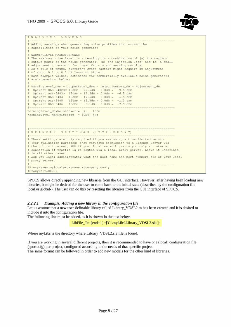
2.2.2 Using Configuration File (“spocs.cfg”) The configuration file contains information about the libraries that will be loaded and other parameters already explained in the manual guide of SPOCS. When a new user-definable library is created, it should be included in the configuration file in order to avoid loading this library every time SPOCS is opened (by means of the GUI of SPOCS). The format when adding a user-definable library is shown in the configuration file. Comments in this configuration file start with the symbol “%.The configuration file, when it is open, looks like:

CONTENTS OF <INSTALLDIR>\SPOCS.CFG

%============================================================================== % C O N F I G U R A T I O N F I L E F O R S P O C S %============================================================================== % Specify the files that contain the user-defined libraries % %------------------------------------------------------------------------------ % C O N F I G U R A T I O N S E T T I N G S %------------------------------------------------------------------------------ Level ='Advanced'; %must be one of 'Basic', 'Advanced', 'Expert' Logging='Screen'; %must be one of 'None', 'Screen', 'File' LogFile='spocs.log'; %must be a valid filename LogLevel='Minimal'; %must be one of 'Minimal', 'Limited', 'Verbose' UnitsLen='meter'; %must be one of 'meter','km','inch','feet','yard','kft','mile'


/ 27

%------------------------------------------------------------------------------ % D E F A U L T S C E N A R I O V A L U E S %------------------------------------------------------------------------------ % NEXT and Equal-Level FEXT are a measure for the (frequency dependent) % crosstalk coupling between the wire pairs. A universal or standardized % value does not exist, since the values are cable dependent % Commonly used values are predefined below, % % Uncomment the lines that matches your preferences, or add other defaults %------------------------------------------------------------------------------ % --- Common values for European studies Cable_NEXT = -50.0; % in dB, at 1MHz Cable_ELFEXT= -45.0; % in dB, at 1MHz and 1 km % % --- Common values for North American studies(T1.417, Annex A.3.2.1.2 and A.3.2.2); %Cable_NEXT = 10*log10(8.536e-15 * (1e6)^(3/2)); % -50.6875 dB(1MHz) %Cable_ELFEXT= 10*log10(7.74e-21 * (1e6)^2 * (1e3/feet)); % -45.9527 dB(1MHz,1km) %------------------------------------------------------------------------------ % D E F A U L T D I R E C T O R I E S %------------------------------------------------------------------------------ % Define the directories where SPOCS writes its output files like % scenarios or noise profiles. It will be ignored if the specified % directory could not be found, % % % predefined variables: % ProgDir contains the program directory, where "spocs.exe" is % CurrDir contains the current directory % examples: % DirScenarios =''; %use current directories % DirScenarios ='C:\User\MyScenarios\'; % DirScenarios =[ProgDir, 'MyScenarios\']; % DirProfiles =[ProgDir, 'Output\MyProfiles\']; % DirLicenses ='C:\User\Secrets\MySpocsLicenses\'; % DirLicenses =[ProgDir,'MyLicenses\']; %------------------------------------------------------------------------------ DirProfiles =''; DirScenarios=''; DirLicenses =''; %------------------------------------------------------------------------------ % L I B R A R I E S (only *.sla) %------------------------------------------------------------------------------ % Adding user-defined libraries. (usually with extention "*.sla"). % Protected libraries (of type "*.slb") cannot be loaded in this way, % and will always be rejected % % Some Predefined variables: % ProgDir contains the program directory, where "spocs.exe" is % CurrDir contains the current directory % % You can load multiple libraries as follows: % LibFile_Traend+1 =[ProgDir,'Libs\MyTransmitters_Part1.sla']; % LibFile_Traend+1 =[ProgDir,'Libs\MyTransmitters_Part2.sla']; % LibFile_Traend+1 =[ProgDir,'Libs\MyTransmitters_Part3.sla']; % % Uncomment the lines below if you want to load the example libraries % on start-up, and keep them after a library reset %------------------------------------------------------------------------------ %LibFile_Traend+1 =[ProgDir,'Examples\examples_UserLibs\Example_transmitterlib.sla']; %LibFile_Recend+1 =[ProgDir,'Examples\examples_UserLibs\Example_receiverlib.sla']; %LibFile_Loopend+1=[ProgDir,'Examples\examples_UserLibs\Example_cablelib.sla']; %LibFile_PBOend+1 =[ProgDir,'Examples\examples_UserLibs\Example_PBOlib.sla']; %------------------------------------------------------------------------------


/ 27

% W A R N I N G L E V E L S %------------------------------------------------------------------------------ % Adding warnings when generating noise profiles that exceed the % capabilities of your noise generator % % WARNINGLEVEL_MAXNOISEPOWER % The maximum noise level in a testloop is a combination of (a) the maximum % output power of the noise generator, (b) the injection loss, and (c) a small % adjustment to account for crest factors and warning margins. % As a rule of thumb, different crest factors might require an adjustment % of about 0.1 to 0.3 dB lower or higher. % Some example values, estimated for commercially available noise generators, % are summarized below: % % WarningLevel_dBm = OutputLevel_dBm - InjectionLoss_dB - Adjustment_dB % Spirent DLS-5402DC 13dBm - 22.5dB - 0.0dB = -9.5 dBm % Spirent DLS-5403D 13dBm - 19.5dB - 0.0dB = -6.5 dBm % Spirent DLS-5404 13dBm - 17.5dB - 0.0dB = -4.5 dBm % Spirent DLS-5405 13dBm - 15.3dB - 0.0dB = -2.3 dBm % Spirent DLS-5406 13dBm - 5.1dB - 0.0dB = +7.9 dBm %------------------------------------------------------------------------------ WarningLevel_MaxNoisePower = -7; %dBm WarningLevel_MaxNoiseFreq = 30E6; %Hz %------------------------------------------------------------------------------ % N E T W O R K S E T T I N G S (H T T P - P R O X Y) %------------------------------------------------------------------------------ % These settings are only required if you are using a time-limited version % (for evaluation purposes) that requests permission to a Licence Server via % the public internet, AND if your local network grants you only an internet % connection if traffic is re-routed via a local proxy server. Leave it undefined % in all other cases. % Ask you local administrator what the host name and port numbers are of your local % proxy server. %------------------------------------------------------------------------------ %ProxyName='mylocalproxyname.mycompany.com'; %ProxyPort=8080; SPOCS allows directly appending new libraries from the GUI interface. However, after having been loading new libraries, it might be desired for the user to come back to the initial state (described by the configuration file –local or global-). The user can do this by resetting the libraries from the GUI interface of SPOCS.

2.2.2.1 Example: Adding a new library in the configuration file Let us assume that a new user-definable library called Library_VDSL2.m has been created and it is desired to include it into the configuration file. The following line must be added, as it is shown in the text below.

LibFile_Traend+1=['C:\myLibs\Library_VDSL2.sla']; Where myLibs is the directory where Library_VDSL2.sla file is found. If you are working in several different projects, then it is recommended to have one (local) configuration file (spocs.cfg) per project, configured according to the needs of that specific project. The same format can be followed in order to add new models for the other kind of libraries.


/ 27

3 Transmitter Library

3.1 Quick Start- Example 1- Downstream of an ADSL2+ system This example shows how to add a transmitter library into SPOCS. A table containing the PSD levels versus the frequency is introduced, typically according to the information given in the standard. Although there are several parameters that can be configured in the transmitter, only a few are needed to establish a new model. The rest of the parameters are taken by default when the REQUIRED LINE is added.

3.2 Fields of the Q structure As it was briefly discussed in the quick example for the transmitter library, there are several fields that are attached to each transmitter model. All these fields are put together in the Q structure. Sometimes, depending on the model to be created, not all these fields are needed (some are taken by default in SPOCS).

Example 1, of the specification of an ADSL2+ transmitter model %.............................................................................. Q.Name = 'TPL.dn:ADSL2+.Example'; Q.Model = 'SpecMask'; % Describes the spectrum method Q.Args1 = 'log:dB'; % meaning that the scale is logarithmic., Y array in dBm/Hz % other possibilities are: % -‘lin:dB’ à linear scale, PSD array in dBm/Hz % -‘log:log’ à log scale, √PSD array in V/sqrt(Hz) %.............................................................................. % table PSD levels versus Frequency (most commonly as indicated in the standard) table = [ [ 0, -101] [ 3.999, -101] [ 4, -96] [ 25.875, -40] [ 1104, -40] [ 1622, -50] [ 2208, -51.3] [ 2500, -62.9] [ 3001.5, -83.5] [ 3175, -100] [ 3750, -100] [ 4545, -110] [ 7225, -112] [ 30000, -112] ]; % Design impedance of system Q.Rs = 100; % Specify Frequency in Hertz Q.f = 1e3*table(:,1); % Specify PSD in dBm/Hz Q.P = table(:,2); % Free form string for comments Q.Info = 'ADSL2+ Template (ADSL2+/A)'; % Higher values indicate more experimental templates. Q.Expert = 0; % REQUIRED LINE to add model Q to library, and to prepare new Q [DATA,Q] = AddPSD(DATA,Q);


/ 27

Qout structure Description

Qout.Name Name of the model

Qout.Expert1 Level of maturity of the model, - 0 high - 4 experimental

Qout.Model Describes the spectrum method Qout.Args Contains several parameters according to the

model. Qout.Parms Contains several parameters according to the

model. Qout.Rs Impedance ( In Ohms) Qout.f Frequency array ( In Hz) Qout.P Power array ( in dBm/ Hz) Qout.Info Free string to describe the model Qout.Cpts To activate the feature of synchronizing with the

counterpart. Table 1: Description of the Qout structure

In order to create a new transmitter model, it is necessary to know the meaning of the Qout.Model field. There are several options for the Qout.Model field. These are presented in Table 2.

Only expert levels that are less or equal than 4 are visible in SPOCS.

QoutModel Description SpecMask Mostly used by inserting a table containing the

PSD levels and the frequency points (includes corner-points), according to the standard or any user-definable option. Q.Args = interpolation-type or Q.Args = fcutoff, interpolation-type1, interpolation-type2 See example 1 and 2

VDSL2_Template Basically it lowers the PSD mask by 3.5 dB. Q.Args = spectral mask, total power, used bands See example 3

NewSpecFilt Q.Args = U0, spectrum-type, Fdip, filter_1,filter_2,U_floor See example 4

SDSL_ETSI QArgs = data-rate, K_sdsl, Factors, Typ where Factors contains 3 fields. See example 5

Cross-Reference Makes a reference to another model. It works like an alias. See example 6

Table 2: Description of the Qout Model field

3.3 Example 2 - Working with VDSL2 - Using SpecMask As VDSL2 has several frequencies ranges and it might use several upstream and downstream bands, using up to 30 MHz (theoretically), there are regions where the spectra can be visualized in a logarithmic way and others


/ 27

(high frequencies) where it has to be switched to linear scale. This is configured in the Q.Args field and it is one of the differences with the previous example. The configuration of the rest of the fields is very similar.

Example 2, of the specification of a VDSL2 transmitter model %.............................................................................. Q.Name = 'MSK.up:VDSL2.Example'; Q.Model = 'SpecMask'; Q.Args = 2825000, 'log:dB', 'lin:dB'; % Meaning that till cut-off frequency of 2825000 will interpolate in a % logarithmic way and after that value will do it in a linear way. % This is established in the standard and implemented in SPOCS % libraries as well. %.............................................................................. table = [ [ 0, -97.5] [ 3.999, -97.5] [ 4, -92.5] [ 25.875, -34.5] [ 50, -34.5] [ 80, -34.5] [ 120, -34.5] [ 138, -34.5] [ 243, -93.2] [ 686, -100] [ 783, -100] [ 2825, -100] [ 2999.999, -80] [ 3000, -56.5] [ 3575, -56.5] [ 3749.999, -56.5] [ 3750, -56.5] [ 5099.999, -56.5] [ 5100, -80] [ 5275, -100] [ 5375, -100] [ 6875, -100] [ 7049.999, -100] [ 7050, -100] [ 8325, -100] [ 8499.999, -100] [ 8500, -100] [ 10000, -100] [ 11999.999, -100] [ 12000, -100] [ 12175, -100] [ 14350, -100] [ 14351, -100] [ 14526, -100] [ 30000, -100] ]; % Design impedance of system Q.Rs = 100; % Specify Frequency in Hertz Q.f = 1e3*table(:,1); % Specify PSD in dBm/Hz Q.P = table(:,2); % Free form string for comments Q.Info = 'VDSL2 Mask, ITU G.993.2 (AR-draft, 2005-12)'; % Higher values indicate more experimental templates. Q.Expert = 3; % REQUIRED LINE to add model Q to library, and to prepare new Q [DATA,Q] = AddPSD(DATA,Q);


/ 27

3.4 Example 3- Working with VDSL2 - Using VDSL2_Template When using VDSL2_Template, the goal consists of reducing the given mask by 3.5 dB. In other words, it is used to derive a VDSL2 PSD template from an existing VDSL2 PSD mask.

Example 3a, of the specification of a VDSL2 transmitter model %.............................................................................. Q.Name = 'TPL.up:VDSL2.Example'; %.............................................................................. Q.Model = 'VDSL2_Template'; %.............................................................................. % Signals that the library should construct a template from a provided mask Q.Args = 'MSK.up:VDSL2.Example'; % from this mask, the template will be created. % It has to be an existing model. % free string for comments Q.Info = 'VDSL2 Mask, Example'; % Higher values indicate more experimental models. Q.Expert = 3; % REQUIRED LINE to add model Q to library, and to prepare new Q [DATA,Q] = AddPSD(DATA,Q); On top of that, it is possible to add some other arguments to the VDSL2 Template model. These are described in table 3.

Argument (Q.Args) Description VDSL2mask Name of the existing MASK PowerLimit Maximum power used Bands Bands to be used. The format is explained with

the following examples. [0, 1, 2] for using US0,US1 and US2 [1, 2] for using DS1 and DS2 [0, 2] for using US0 and US2, etc.

DPBOESEL Insertion loss in dB at 300 kHz. Exchange-Side Electrical length for PSD shaping (downstream only). See [6] for more details

DPBOMUS PSDfloor (in dBm/Hz) that determines the MUF, (the Maximum Usuable Frequency. Maximum Usuable Signal for PSD shaping (downstream only). See [6] for more details

A, B, C ABC polynomial parameters for the cable in use. See [6] for more details

Table 3: Description of Q.Args field An example showing the use of these additional arguments is presented.

Example 3b, of the specification of an VDSL2 transmitter model %.............................................................................. Q.Name = 'TPL.up:VDSL2.Example2'; %.............................................................................. Q.Model = 'VDSL2_Template2'; %.............................................................................. % Signals that the library should construct a template from a provided mask % from this mask, the template will be created. It has to be an existing model. Q.Args = 'MSK.up:VDSL2.Example2',14.5,[0,1,2];


/ 27

% % Here , we have added the power constraint of 14.5 dBm and the use of 3 upstream bands, US0, % US1 and US2. % free string for comments Q.Info = 'VDSL2 Mask, Example2'; % Higher values indicate more experimental models. Q.Expert = 3; % to synchronize with the counterpart Q.Cpts.Tra = 'TPL.dn:VDSL2.B8-5-(998-M2x-M)'; Q.Cpts.Rec = 'VDSL2/B.up[B8]-(expert guess)'; % REQUIRED LINE to add model Q to library, and to prepare new Q [DATA,Q] = AddPSD(DATA,Q);

3.5 Example 4- Working with HDSL - Using NewSpecFilt This example introduces new features to be used when creating a transmitter model. For instance, the use of low-pass and high-pass filters is shown leading to another way of using the Q.Args field. Please refer to the ETSI SpM-2 standard [1] for more details.

Example 4, of the specification of an HDSL transmitter model %.............................................................................. Q.Name = 'TPL:HDSL.2B1Q/2.Example'; %.............................................................................. % ISDN.2B1Q template, as defined in the SpM-2 standard % TR 101 830-2 (2005-10), par 4.8 % BvdH, November 2005 %.............................................................................. % Design impedance of system Rs = 135 ; % Establishing the Power Level P_dBm = 14 ; % Symbol Frequency Fdip = 584E3 ; % Creates low and high pass filters FL = 3e3 ; % high pass filter, 3dB cut-off frequency NL = 1 ; % high pass filter, order of the filter FH1 = 0.68*Fdip ; % low pass filter, 3dB cut-off frequency NH1 = 4 ; % low pass filter, order of the filter q = 1.1915 ; % use to relate power level to voltage % PSD floor level P_floor = -133 ; % Converting dBm to volts, main signal U0 = sqrt(Rs*10^(P_dBm/10)*1e-3*q) ; % Converting dBm to volts, floor signal U_floor = sqrt(Rs*10^(P_floor/10)*1e-3) ; % Model Type to be used for the spectra Q.Model = 'NewSpecFilt' ; % Arranging the parameters in Q structure Q.Rs = Rs ; Q.Args = U0, '2B1Q', Fdip, 'FilterLP','ButtAbs', FH1, NH1,... 'FilterHP','ButtAbs', FL, NL, U_floor; % free string for comments Q.Info = 'HDSL.2B1Q Template (2-pair), TR 101 830-2 (2005-10)';


/ 27

% Higher values indicate more experimental models. Q.Expert = 0; % REQUIRED LINE to add model Q to library, and to prepare new Q [DATA,Q] = AddPSD(DATA,Q); % Add Q to PSD, and create new Q...

3.6 Example 5- Working with SDSL - Using SDSL_ETSI This is a special model that requires some additional explanation. Let us briefly describe the input parameters. For more details about the definition of the parameters used in this example, please refer to ETSI SpM-2 standard, pp 18 [1].

Parameter Description DataRate The data rate specified in kbit/s., and used to derive the line rate as internal

parameter, via LineRate = DataRate + 8 k K_sdsl A scaling factor, as defined in the ETSI standard Factors An array that contains 3 fields, eg. Factors=[1/3, 1/2, 6], being used to derive

various internal parameters Fsym (= symbol rate), F0_h (= 3 dB break frequency of low-pass filter) Nh (= filter order) These values are as follows derived from the 3 factors: Fsym = LineRate * Factor1 F0_h = Fsym * Factor2 Nh = Factor3

Typ A string that specifies how the spectra are to be derived ‘nominal’, as defined in ETSI SDSL standard (and ITU) ‘template_120’, as defined in ETSI SpM-2 standard 'nominal_enhanced', as defined for enhanced SDSL in ETSI (and ITU)

Example 5, of the specification of an SDSL transmitter model %.............................................................................. Q.Name = 'TPL:SDSL.512.s.Example'; %.............................................................................. % Nominal SDSL spectrum according to ETSI SpM standard (part 2, October 2005), % [U,Rs]=SDSL_ETSI(DataRate,K_sdsl,Factors,Typ); %.......................................................................... Q.Model = 'SDSL_ETSI'; % Design impedance of system Q.Rs=135; % Input Arguments Q.Args = 512E3, 7.86, [1/3, 1/2, 6],'template_120'; % free string for comments Q.Info = 'SDSL Template, TR 101 830-2 (2005-10)'; % Higher values indicate more experimental models. Q.Expert = 0; % REQUIRED LINE to add model Q to library, and to prepare new Q [DATA,Q] = AddPSD(DATA,Q);


/ 27

3.7 Example 6- Working with ADSL - Using Cross-Reference The cross reference means no modification in some previous model. This is why this new model references the other plus only a new field of “Q.Info” that might be created for special studies.

Example 6, of the specification of an ADSL transmitter model %..................................................................... Q.Name = 'TPL.up:ADSL/A-(G992.1,FDD)'; %..................................................................... % ADSL FDD (reduced NEXT), upstream. This is the wideband PSD mask, % that can be used as template % Based on Annex A.2.4 of ITU G.992.1 (1999-07) % Note: there is no distinction between FDD/EC for the upstream... %..................................................................... Q.Model = 'Cross_Reference'; % % Selecting the model this new model will be based on Q.Args1 = 'TPL.up:ADSL/A-(G992.1)'; % free string for comments Q.Info = 'ADSL Template, derived from ITU G.992.1 (1999-07)'; % Higher values indicate more experimental models. Q.Expert = 1; % REQUIRED LINE to add model Q to library, and to prepare new Q [DATA,Q] = AddPSD(DATA,Q); % Add Q to PSD, and create new Q...


/ 27

4 Loop Library

Currently SPOCS supports a big amount of cable models for both European and North American regions. However, in order to provide flexibility to the user and adjust its simulation scenario as much as possible to the reality, SPOCS also allows the insertion of new cable models. For more details about the modelling of these or any other European cables and a better understanding of the different parameters herein used, please refer to ETSI “Cable reference models for simulating metallic access networks”.

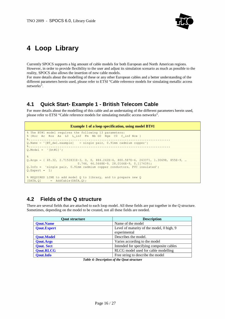
4.1 Quick Start- Example 1 - British Telecom Cable For more details about the modelling of this cable and an understating of the different parameters herein used, please refer to ETSI “Cable reference models for simulating metallic access networks”.

Example 1 of a loop specification, using model BT#1 % The BT#1 model requires the following 13 parameters: % Roc Ac Ros As L0 L_inf Fm Nb G0 Nge C0 C_inf Nce %.............................................................................. Q.Name = '[BT_dw1.example] = single pair, 0.91mm cadmium copper'; %.............................................................................. Q.Model = '[bt#1]'; % Q.Args = 65.32, 2.7152831E-3, 0, 0, 884.242E-6, 800.587E-6, 263371, 1.30698, 855E-9, … 0.746, 46.5668E-9, 28.0166E-9, 0.117439; Q.Info = 'single pair, 0.91mm cadmium copper conductors, PVC insulated'; Q.Expert = 1; % REQUIRED LINE to add model Q to library, and to prepare new Q [DATA,Q] = AddCable(DATA,Q);

4.2 Fields of the Q structure There are several fields that are attached to each loop model. All these fields are put together in the Q structure. Sometimes, depending on the model to be created, not all these fields are needed.

Qout structure Description Qout.Name Name of the model Qout.Expert Level of maturity of the model, 0 high, 9

experimental Qout.Model Describes the model. Qout.Args Varies according to the model Qout. Sect Intended for specifying composite cables Qout.RLCG RLCG model used for cable modelling Qout.Info Free string to describe the model

Table 4: Description of the Qout structure


/ 27

4.3 Example 2- The Deutsche Telecom Cable DTAG #1 In order to understand the parameters involved here, it is highly recommended to check the standard previously cited.

Example 2 of a loop specification, using model DTAG#1 % The DTAG#1 model requires the following 13 parameters: % FFmin, FFmax, Ka1, Ka2, Ka3, Kb1, Kb2, Kz1, Kz2, Kz3, Kx1, Kx2, Kx3 %.............................................................................. Q.Name = '[DTAG_35.example] = 0.35mm cable (Germany)'; % name of the model Q.Model = '[dtag#1]'; % parameters corresponding to the cable model Q.Args = [0.075,0.5,5]*1E6, [0.5,5,30]*1E6, [9.4,2.4,15.9], [13.2,19.9,11.2], [0.97,0.54,0.69],… 34.2, 2.62, 132, 5.0, 0.73, 0.050, 0.024, 0.87; % free string for comments Q.Info = 'Deutsche Telecom cable 0.35mm'; % level of expertise Q.Expert = 1; % REQUIRED LINE to add model Q to library, and to prepare new Q [DATA,Q] = AddCable(DATA,Q);

4.4 Example 3- Composite loop consisting of 2 sections and 1 single bridge tap

It is possible to create composite loops. When this is the goal, then the field called “Q.Sect” takes a relevant role.

LT

L2

NTL1 L3

Figure 3: Topology with only 1 bridge tap The composite loop is shown in figure 3: it consists of two sections and one bridge tap. The bridge tap is located at L1 meters from the LT, and at L3 meters from the NT. As a consequence, the total length of the loop is L = L1 + L3. The length of the bridge tap itself is L2.


/ 27

Example 3 of a loop specification with a single bridge tap % This file contains an example of how the user can add a cable model with a % bridge tap in it. The various lengths in the model can be modified. % % In the current file, the lengths L2 and L3 are specified. % The total length L is speficied via the GUI, and the program calculates L1 = L - L3. % Note: for this model to make sense, the user must choose L > L3. % L2 AND L3 ARE PARAMETERS THAT CAN BE CHANGED BY THE USER: feet = 0.3048; % defines a constant: one foot equals 0.3048 meters L2 = 250*feet; % set length of bridge tap (must be in meters!) L3 = 750*feet; % set distance between bridge tap and NT (must be in meters!) %.............................................................................. Q.Name = '[MyBridgeTap] = AWG26, loop with single bridgetap'; %.............................................................................. Q.Model = '[LOOP]'; Q.Sect1.xTU = 'LT'; % put LT at left hand side Q.Sect3.xTU = 'NT'; % put NT at right hand side %Type of each legs Q.Sect1.Name='[AWG26]'; % first leg is of type 'AWG26' Q.Sect2.Name='[AWG26]'; % second leg (the bridge tap) is of type 'AWG26' Q.Sect3.Name='[AWG26]'; % third leg is of type 'AWG26' % Type of the different sections that are going to be created Q.Sect1.Type='casc'; % first leg is a part of the attenuation path Q.Sect2.Type='tap'; % second leg is a bridge path Q.Sect3.Type='casc'; % third leg is a part of the attenuation path % Length of the corresponding section Q.Sect1.Len ='frac_len', 1; % This results in L1 = L - L3 (with L specified via the GUI) Q.Sect2.Len ='abs_len', L2; % Length of bridge tap (user definable) Q.Sect3.Len ='abs_len', L3; % Length of the third leg (user definable) % free string for comments Q.Info = 'Example of a cable with one bridge tap'; % level of expertise Q.Expert = 1; % REQUIRED LINE to add model Q to library, and to prepare new Q [DATA,Q] = AddCable(DATA,Q);

4.5 Example 4- Composite loop consisting of 2 sections and 2 bridge taps

This example is based on the model ETSI.HDSL#6 as given in the standard [2]. The topology to be created is reproduced here for illustration purposes.

500 m

500 m

0,4 mm PE

0,4 mm PE

NT

2/7

5/7

LT

Sect1 = tap Sect3 = tap

Sect2 = casc Sect4 = casc

Figure 4: Composite cable for ETSI.HSDL#6


/ 27

Example 3 of a loop specification with 2 sections and 2 bridge taps %.............................................................................. Q.Name = '[ETSI.HDSL#6.Example] = standard testloop: BridgeTaps/0.40PE'; %.............................................................................. % Insertion loss, for Y=31dB @ 150 kHz, according to % ETSI HDSL spec: TS 101 135 V1.5.1 (1998-11), app A.2 % IL=27.0 % ==> L6=[Len*0.28571, Len*0.71429]; sum(L6)/Len Q.Model='[LOOP]'; % Composite Loop Q.Sect1.xTU = 'NT'; Q.Sect4.xTU = 'LT'; % Name of the model Q.Sect1.Name='[ETSI/HDSL:0.40PE]'; % 120 ohm Q.Sect2.Name='[ETSI/HDSL:0.40PE]'; % 120 ohm Q.Sect3.Name='[ETSI/HDSL:0.40PE]'; % 120 ohm Q.Sect4.Name='[ETSI/HDSL:0.40PE]'; % 120 ohm % Type of the different sections that are going to be created Q.Sect1.Type='tap'; Q.Sect2.Type='casc'; Q.Sect3.Type='tap'; Q.Sect4.Type='casc'; % Length of the corresponding section Q.Sect1.Len ='abs_len' 500; Q.Sect2.Len ='frac_attn150' 2/7; Q.Sect3.Len ='abs_len' 500; Q.Sect4.Len ='frac_attn150' 5/7; % level of expertise Q.Expert = 0; % Free string Q.Info = 'ETSI HDSL spec: TS 101 135 V1.5.1 (1998-11), app A.2'; % REQUIRED LINE to add model Q to library, and to prepare new Q [DATA,Q] = AddCable(DATA,Q);


/ 27

5 PBO Library

It is possible to apply power back-off in the upstream as well as in the downstream. This will be realized according to the name of the PBO model to be used.

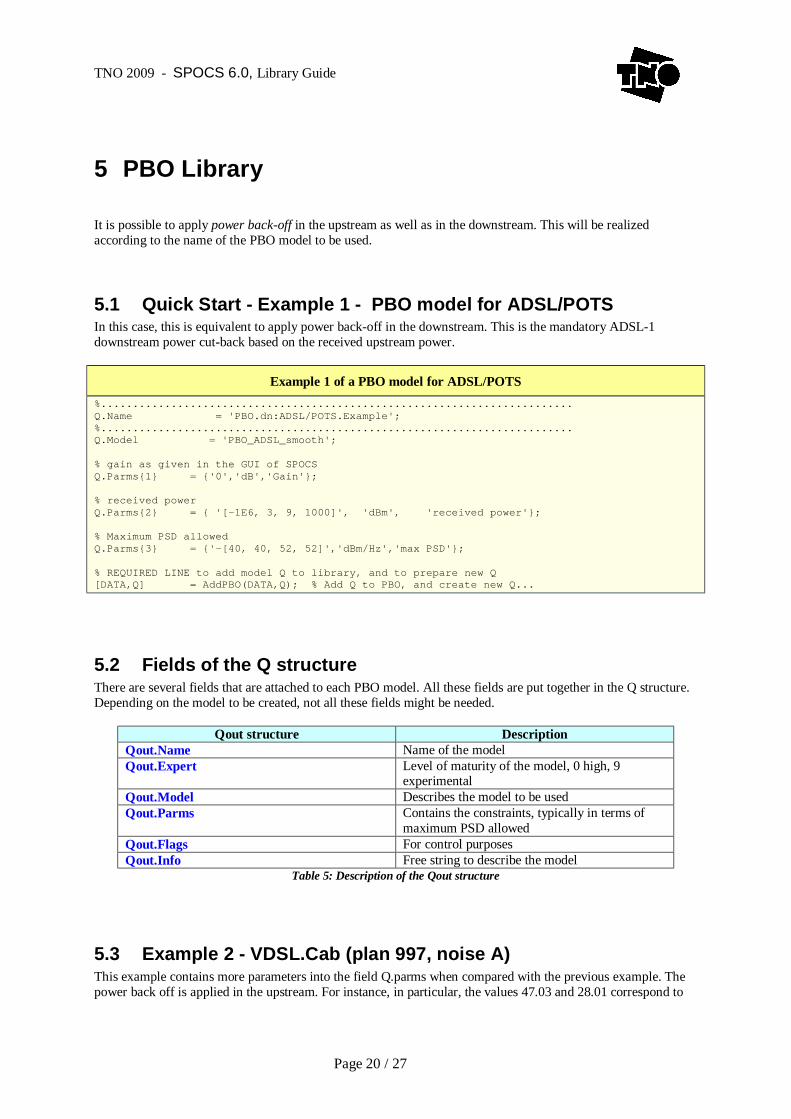
5.1 Quick Start - Example 1 - PBO model for ADSL/POTS In this case, this is equivalent to apply power back-off in the downstream. This is the mandatory ADSL-1 downstream power cut-back based on the received upstream power.

Example 1 of a PBO model for ADSL/POTS %.......................................................................... Q.Name = 'PBO.dn:ADSL/POTS.Example'; %.......................................................................... Q.Model = 'PBO_ADSL_smooth'; % gain as given in the GUI of SPOCS Q.Parms1 = '0','dB','Gain'; % received power Q.Parms2 = '[-1E6, 3, 9, 1000]', 'dBm', 'received power'; % Maximum PSD allowed Q.Parms3 = '-[40, 40, 52, 52]','dBm/Hz','max PSD'; % REQUIRED LINE to add model Q to library, and to prepare new Q [DATA,Q] = AddPBO(DATA,Q); % Add Q to PBO, and create new Q...

5.2 Fields of the Q structure There are several fields that are attached to each PBO model. All these fields are put together in the Q structure. Depending on the model to be created, not all these fields might be needed.

Qout structure Description Qout.Name Name of the model Qout.Expert Level of maturity of the model, 0 high, 9

experimental Qout.Model Describes the model to be used Qout.Parms Contains the constraints, typically in terms of

maximum PSD allowed Qout.Flags For control purposes Qout.Info Free string to describe the model

Table 5: Description of the Qout structure

5.3 Example 2 - VDSL.Cab (plan 997, noise A) This example contains more parameters into the field Q.parms when compared with the previous example. The power back off is applied in the upstream. For instance, in particular, the values 47.03 and 28.01 correspond to


/ 27

the values of [a, b] when upstream power back-off is used in US1. And, 54.0 and 19.22 correspond to these values in US2.

Example 2 of a PBO model for VDSL.Cab (plan 997, noise A) %.......................................................................... Q.Name = 'PBO.up:VDSL_E1_Cab.NoiseA.Example'; %.......................................................................... Q.Model = 'PBO_VDSL_stair'; % UPBO properties Q.Parms1 = '0','dB','Gain'; % (a, b) are the UPBO parameters per upstream band % values of a for US1 and US2 Q.Parms2 = '-[0, 47.3, 0, 54.0, 0]', 'dBm/Hz','ref PSD'; % values of b for US1 and US2 Q.Parms3 = '-[0, 28.01, 0, 19.22, 0]', 'dBm/Hz','ref PSD*sqrt(f/1MHz)'; % frequency array Q.Parms4 = ' [0, 3-0.2, 5.1+0.2, 7.05-0.2, 12+0.2, 1000]', 'MHz', 'freq'; % free string for comments Q.Info = 'Upstream PBO, ETSI TS 101 270-1 (VDSL-1, 2003-07)'; % REQUIRED LINE to add model Q to library, and to prepare new Q [DATA,Q] = AddPBO(DATA,Q); % Add Q to PBO, and create new Q...


/ 27

6 Receiver Library

In the same way new transmitter / disturbers models are allowed to be included in SPOCS, receiver models can also be created as well. The same remark applies to the creation of receiver libraries. For instance, the user has to get used to the structure. This can be explained easier with the examples given in this section followed by the description of the fields commonly used when a receiver library is created.

6.1 Quick Start - Example 1 - Creating HDSL.2B1Q/2 Receiver There might be several receiver properties. The user can set up the most relevant properties for that particular model and the others will be configured by default for SPOCS.

Example 1 of a receiver model for HDSL.2B1Q/2 %........................................................................ Q.Name = 'HDSL.2B1Q/2.Example' ; Q.Class = 'ETSI_HDSL_2B1Q' ; Q.Args = 2048E3,2 ; % Shannon Gap and Receiver Noise Q.Parms2 = '9.5', 'dB', 'Gap'; Q.Parms3 = '-140', 'dBm@Rv', 'Noise'; % These parameters are chosen very high to assume ideal case Q.Parms4 = '200', 'dB', 'EchoSup'; Q.Parms5 = '200', 'dB', 'DistSup'; % Higher values indicate more experimental models. Q.Expert = 3; % REQUIRED LINE to add model Q to library, and to prepare new Q [DATA,Q] = AddReceiver(DATA,Q); % Add Q to REC, and create new Q...

6.2 Review of Receiver Models In the receiver library, as briefly explained in SPOCS user-guide, there are 4 main models to be used in the Qout.Model field.

Model Description Shannon (Shifted Shannon) Generic Model. It is line code independent PAM Dedicated to line-codes using Pulse Amplitude Modulation CAP Dedicated to line-codes using quadrature modulation DMT Dedicated to line-codes using multiple discrete tones

Table 6: Model Types for Receiver systems When creating a new receiver model, there are several properties that should be taken into account. This list provides a guide for the user in order to be aware of the properties according to the type of line code that will be used.

PROPERTIES SHANNON PAM CAP DMT Gap x x x x Noise x x x x EchoSup x x x x DistSup x x x x


/ 27

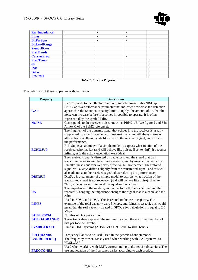
Rn (Impedance) x x x x Lines x x x BitPerSym x x BitLoadRange x SymbolRate x FreqBands x CarrierFreq x FreqTones x dF x INP x Delay x EOCOH x

Table 7: Receiver Properties The definition of these properties is shown below.

Property Description GAP

It corresponds to the effective Gap in Signal-To Noise Ratio NR-Gap. SNR-Gap is a performance parameter that indicates how close the detection approaches the Shannon capacity limit. Roughly, the amount of dB that the noise can increase before it becomes impossible to operate. It is often represented by the symbol ΓdB.

NOISE

Corresponds to the receiver noise, known as PRN0_dB (see figure 2 and 3 in Annex C of the SpM2 reference).

ECHOSUP

The fragment of the transmit signal that echoes into the receiver is usually suppressed by an echo canceller. Some residual echo will always remain after echo cancellation, adds like noise to the received signal, and reduces the performance. EchoSup is a parameter of a simple model to express what fraction of the received echo has left (and will behave like noise). If set to “Inf”, it becomes infinite, as if the echo cancellation were ideal

DISTSUP

The received signal is distorted by cable loss, and the signal that was transmitted is recovered from the received signal by means of an equalizer. Usually, these equalizers are very effective, but not perfect. The restored signal will always differ a slightly from the transmitted signal, and this will also add noise to the received signal, thus reducing the performance. DistSup is a parameter of a simple model to express what fraction of the transmitted signal is not recovered (and will behave like noise). If set to “Inf”, it becomes infinite, as if the equalization is ideal

RN

The impedance of the modem, and in use for both the transmitter and the receiver. Changing the impedance changes the signal loss in a cable and the echo

LINES

Used in SDSL and HDSL. This is related to the use of capacity. For example, if the total capacity were 5 Mbps, and, Lines is set to 2, this would mean that the real capacity treated in SPOCS for calculations is equal to 2.5 Mbps.

BITPERSYM Number of Bits per symbol. BITLOADRANGE These two values represent the minimum as well the maximum number of

bits per tone per symbol. SYMBOLRATE

Used in DMT systems (ADSL, VDSL2). Equal to 4000 baud/s.

FREQBANDS Frequency Bands to be used. Used in the generic Shannon model. CARRIERFREQ

The frequency carrier. Mostly used when working with CAP systems, i.e. HDSL.CAP

FREQTONES

Used when working with DMT, corresponding to the set of sub-carriers. The use and location of the freq-tones varies according to each product


/ 27

supporting DMT. DF

The delta frequency is the spacing between DMT carriers Common value is 4,3125KHz, though in VDSL2 systems it may change to 8,625 KHz when high frequencies are used

INP

Impulse Noise Protection: This is a parameter used in ADSL2+ in order to deploy a protection mechanism for the effect of impulse noise. There are several tables on ref [3,4] from which the user can choose the symbols to be used in conjunction with the delay. Changing INP will change the amount of overhead (difference between the LineRate and the DataRate)

DELAY

This is a parameter used in ADSL2+ and provides in conjunction with INP the mechanism to protect the system against Impulse Noise effect. Changing Delay will change the amount of overhead (difference between the LineRate and the DataRate)

EOCOH

Embedded Operational Channel-OverHead: This parameter has a range from 8-to-64 Kbps and is used for exchanging messages between the modems

Table 8: Receiver Properties Description

6.3 Fields of the Q structure There are several fields that are attached to each receiver model. All these fields are put together in the Q structure. Depending on the model to be created, not all these fields might be needed.

Qout structure Description Qout.Name Name of the model Qout.Expert Level of maturity of the model, 0 high, 9 experimental Qout.Class The big group where the new model will belong to Qout.Args Varies according to the type of model Qout.Info Free string to describe the model Qout.Parms Contains different properties of the model Qout.Flags For Control purposes Qout.Calc Describes how the bit rate (line and data rate) is calculated. Assumes 5% of

overhead between line rate and data rate by default Qout.Goal Decides whether bit rate or margin will be calculated. Bit rate can be given

by line rate or data rate. Margin can be given by signal or noise margin. Table 9: Description of the Qout structure

6.4 Example 2- Creating ADSL2+/A.dn[EC] Receiver

Example 2 of a receiver model for ADSL2+ %........................................................................ Q.Name = 'ADSL2+/A.dn[EC].Example'; % BvdH, 08/07/2005 Q.Class = 'ADSL2'; % Q.Args = 10240E3; % Receiver Properties Q.Parms2 ='6.75', 'dB', 'Gap'; Q.Parms3 ='-135', 'dBm@Rv', 'Noise'; Q.Parms4 ='2', 'Symbols', 'INP'; Q.Parms5 ='8', 'ms', 'Delay'; Q.Parms6 ='[7:63,65:511]', '', 'FreqTones'; % Higher values indicate more experimental models.


/ 27

Q.Expert = 1; % free string for comments Q.Info = 'Expert guess for ADSL2+ receiver model; not in a standard yet'; % REQUIRED LINE to add model Q to library, and to prepare new Q [DATA,Q] = AddReceiver(DATA,Q); % Add Q to Rexpert guess, and create new Q...

6.5 Example 3- ADSL/POTS in the downstream -FDD

Example 3 of a receiver model for ADSL/POTS in downstream %.............................................................................. Q.Name = 'ADSL/POTS.dn[FDD].Example'; Q.Class = 'ADSL'; % Q.Args = 2048E3; % Receiver Properties Q.Parms2 = '8.0', 'dB', 'Gap'; Q.Parms3 = '-140', 'dBm@Rv', 'Noise'; Q.Parms4 = 'inf' , 'dB', 'EchoSup'; Q.Parms5 = 'inf', 'dB', 'DistSup'; Q.Parms6 = '[33:63,65:255]', '', 'FreqTones'; % Higher values indicate more experimental models. Q.Expert = 0; % free string for comments Q.Info = 'FDD ADSL over POTS Receiver, TR 101 830-2 (2005-10)'; % REQUIRED LINE to add model Q to library, and to prepare new Q [DATA,Q] = AddReceiver(DATA,Q); % Add Q to REC, and create new Q...


/ 27

7 References

[1] “Transmission and Multiplexing TM; Access Networks; Spectral Management on metallic access networks; Part 2: Technical methods for performance evaluations”, draft ETSI TR 101 830-2 v1.1.1 (2005-09), Sept 22, 2005. [2] Rob Van den Brink, KPN Research, “Realistic ADSL noise models”, contribution to ETSI STC TM6 Meeting, 29 Nov - 3 Dec, 1999. [3] ETSI TS 101 388 v1.3.1 (2002-05), Technical Specification, “Transmission and Multiplexing TM; Access Transmission systems on metallic access cables; Asymmetric Digital Subscriber Line (ADSL) – European specific requirements”. [4] Asymmetric digital subscriber line transceivers 2 (ADSL2), G.992.3 Amendment 2: Amendments to Annex J and new Annexes L and M. [5] Rob Van den Brink, KPN Research. “Cable reference models for simulating metallic access networks”, contribution to ETSI STC TM6 Meeting, (ACCESS TRANSMISSION SYSTEMS ON METALLIC CABLES), 22-26 June, 1998 [6] ITU-T G.997.1, “Physical layer management for digital subscriber line (DSL) transceivers”, February 2006.


/ 27

Annex A: Cable Models

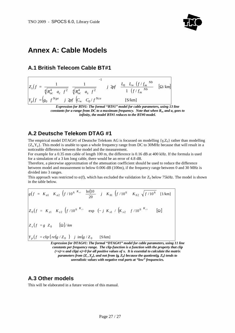
A.1 British Telecom Cable BT#1

( ) ( )( )

[ ]

( ) ( ) ( ) [S/km]/2

//1

/211

00

0

1

4 244 24

ecNegNp

bNm

bNm

soccocs

fCCfjfgfY

kmff

ffLLfj

faRfaRfZ

+⋅⋅+⋅=

Ω

+

⋅+⋅⋅+

⋅++

⋅+=

∞

∞

−

π

π

Expression for BT#1: The formal “BT#1” model for cable parameters, using 13 line constants for a range from DC to a maximum frequency. Note that when Ros and as goes to

infinity, the model BT#1 reduces to the BT#0 model.

A.2 Deutsche Telekom DTAG #1 The empirical model DTAG#1 of Deutsche Telekom AG is focussed on modelling γ,Z0 rather than modelling Zs,Yp. This model is unable to span a whole frequency range from DC to 30MHz because that will result in a noticeable difference between the model and the measurement. For example for a 0.35 mm cable of length 100 m, the difference is 0.16 dB at 400 kHz. If the formula is used for a simulation of a 3 km long cable, there would be an error of 4.8 dB. Therefore, a piecewise approximation of the attenuation coefficient should be used to reduce the difference between model and measurement to below 0.006 dB (100m), if the frequency range between 0 and 30 MHz is divided into 3 ranges. This approach was restricted to α(f), which has excluded the validation for Z0 below 75kHz. The model is shown in the table below.

( ) ( ) ( ) ( )

( ) ( ) ( ) ( ) [ ]

( ) [ ]

( ) ( ) ( ) [S/km]//

/

10//exp10/

[1/km]10/10/2010ln10/

00

0

621

6210

62

61

621

33

3

ZimjZreclipfY

kmZfZ

fKKjfKKfZ

fKfKjfKKf

p

s

Kxx

Kzz

bbK

aa

xz

a

γγ

γ

γ

⋅+=

Ω⋅=

Ω

+⋅−⋅

⋅+=

⋅+⋅⋅+⋅

⋅+=

Expression for DTAG#1: The formal “DTAG#1” model for cable parameters, using 11 line constants per frequency range. The clip-function is a function with the property that clip

(+x)=x and clip(-x)=0 for all positive values of x. It is essential to calculate the matrix parameters from Zs ,Yp, and not from γ, Z0 because the quotientγ, Z0 tends to

unrealistic values with negative real parts at “low” frequencies.

A.3 Other models This will be elaborated in a future version of this manual.

SPOCS 6.0 Library Guide - innovation for life | TNO · P.O. Box 5050 2600 GB Delft The Nederlands...

Documents

Transcript of SPOCS 6.0 Library Guide - innovation for life | TNO · P.O. Box 5050 2600 GB Delft The Nederlands...