Split-Sample Strategies for Avoiding False Discoveries ∗

Michael L. Anderson

UC Berkeley and NBER

Jeremy Magruder

UC Berkeley and NBER

June 30, 2017

Abstract

Preanalysis plans (PAPs) have become an important tool for limiting false discoveries in

field experiments. We evaluate the properties of an alternate approach which splits the data

into two samples: An exploratory sample and a confirmation sample. When hypotheses are

homogeneous, we describe an improved split-sample approach that achieves 90% of the re-

jections of the optimal PAP without requiring preregistration or constraints on specification

search in the exploratory sample. When hypotheses are heterogeneous in priors or intrinsic

interest, we find that a hybrid approach which prespecifies hypotheses with high weights and

priors and uses a split-sample approach to test additional hypotheses can have power gains

over any pure PAP. We assess this approach using the community-driven development (CDD)

application from Casey et al. (2012) and find that the use of a hybrid split-sample approach

would have generated qualitatively different conclusions.

∗Michael L. Anderson is Associate Professor, Department of Agricultural and Resource Economics, University

of California, Berkeley, CA 94720 (E-mail: mlanderson@berkeley.edu). Jeremy Magruder is Associate Profes-

sor, Department of Agricultural and Resource Economics, University of California, Berkeley, CA 94720 (E-mail:

jmagruder@berkeley.edu). They gratefully acknowledge funding from the NSF under Award 1461491, “Improved

Methodologies for Field Experiments: Maximizing Statistical Power While Promoting Replication,” approved in

September 2015. They thank Katherine Casey, Ted Miguel, Sendhil Mullainathan, Ben Olken, and conference and

seminar participants at the Univ of Washington, Stanford, UC Berkeley, and Notre Dame for insightful comments and

suggestions and are grateful to Aluma Dembo and Elizabeth Ramirez for excellent research assistance. All mistakes

are the authors’.

1

1 Introduction

A classic tradeoff in data analysis exists between estimating large numbers of parameters and gen-

erating results that do not reproduce in new samples. In computer science and machine learning

this problem is known as “overfitting;” in biostatistics it manifests itself in “large-scale multiple

testing.” In the past decade it has become a critical issue in empirical microeconomics with the

widespread use of field experiments.1 Researchers designing field experiments often face high

fixed costs in setting up the experiment and low marginal costs in adding additional survey out-

comes. Increasing sample size is expensive, and the samples in many field experiments are too

small to detect anything less than a large effect. Given these constraints and the focus on positive

results in economics and other social sciences (Gerber and Malhotra 2008; Yong 2012), researchers

face strong incentives to test for effects on many outcomes or subgroups and then emphasize the

subset of significant results. Unfortunately this behavior maximizes the chances of “false discov-

eries” (type I errors) that do not replicate in new samples. Although social scientists are becoming

aware of the problem (Miguel et al. 2014), standards have yet to be established to address it.

Limiting false discoveries is an economic problem as well as a statistical one because it must

address the information asymmetry between researchers and reviewers. Though statistical tools

are available for controlling the false discovery rate, most economics papers do not rigorously

test whether their p-values are more extreme than would be expected under the null hypothesis

based on the number of reported results. More importantly, even procedures that control the false

discovery rate (FDR) or familywise error rate (FWER) may be easily gamed by underreporting of

insignificant results; the problem is that the reviewer does not know whether the reported number

of tests performed reflects the true number of tests performed. This problem challenges most

solutions in empirical economics; unless researchers can commit to reliably reporting the full set

of enacted tests, we cannot accurately adjust the p-values of those tests for multiple inference.2

One method of resolving the critical information asymmetry is the use of a preanalysis plan

(PAP). With a PAP, the researcher publicly documents the set of hypotheses that she intends to

test prior to collecting the data. This method follows an approach used for decades in biostatistics

1It is also an issue in many observational studies, but it is difficult to establish when a researcher first had access to

the data in an observational study, and establishing this timeline is critical to any method for limiting false discoveries.2The researcher need not be dishonest; in practice, she herself may not recall all the tests that she has performed.

2

(Simes 1986; Horton and Smith 1999). Casey et al. (2012) established best practices and popu-

larized the use of PAPs among empirical microeconomics using a case of a Community-Driven

Development (CDD) program in Sierra Leone; in that context they prespecified a broad range

of outcomes as potential tests.3 Since that influential study, others have followed this approach,

and grant funders (e.g., International Initiative for Impact Evaluation, or 3ie) are internalizing the

importance of multiple inference and making a PAP a condition for funding.

Despite the track record of PAPs in other fields, serious issues arise with their application in

economics. First, they discourage tests that may generate novel or unexpected findings, as includ-

ing these tests reduces the power of all other tests in a properly specified PAP. Second, they restrict

researchers’ ability to learn from the data and build economic models informed by empirical re-

sults. Much of the analysis in economics proceeds in a sequential fashion. Conditional on one test

rejecting, a researcher may conduct several more tests to understand the mechanisms underlying

the rejection or test for further effects on other outcomes. Specifying an analysis plan that cap-

tures all possible paths by which an analysis may proceed becomes combinatorially impractical

for all but the simplest cases (Coffman and Niederle 2015; Olken 2015). This issue is increas-

ingly important as the field moves from experiments that evaluate a specific program or treatment

to experiments that inform us about the mechanisms underlying an observed treatment effect or

discriminate between different economic models (Card et al. 2011; Ludwig et al. 2011).

This paper develops a split-sample approach to avoiding false discoveries which may be used as

either a complement or an alternative to a preanalysis plan. This approach withholds a fraction of

the data from the researcher in a “confirmation sample.” Researchers conduct exploratory analysis

in the fraction of the data not withheld – the “exploratory sample” – and then register a simple

analysis plan documenting the subset of hypotheses that they wish to validate in the confirmation

sample. In the exploratory sample, researchers can analyze the sample in an unconstrained way,

without need for an algorithm or documentation of the tests that are considered.

One advantage of this approach is that anticipation is unnecessary. In concurrent but indepen-

3While Casey et al. (2012) is arguably the highest profile example of a PAP in empirical microeconomics, it is

not the earliest. For example, Neumark (2001) applied a prespecified research design to observational data from

the Current Population Survey (CPS). To add credibility he submitted the research design to a journal prior to the

publication of the relevant CPS data.

3

dent work, Fafchamps and Labonne (2017) propose a balanced version of this approach (i.e., one

with equally sized exploratory and confirmation samples) and find that it performs well, relative

to a PAP, when researchers identify many hypotheses that they were unable to anticipate or when

expected t-statistics are very large.4 However, the split sample’s flexibility comes at a cost: the

approach loses power relative to a full-sample PAP on hypotheses which were anticipated. For a

balanced approach, this loss in power can be large.

We assess the potential of split-sample methods under two objective functions. First, we con-

sider a researcher who maximizes rejections over a set of ex ante identical hypotheses. We demon-

strate that a researcher with this objective function constructing a PAP would choose to include

every hypothesis in the PAP. To develop the potential of the split-sample method, we propose and

analyze a series of refinements – allocating a majority of the data to the confirmation sample, using

one-sided tests in the confirmation sample, choosing thresholds for passing hypotheses to the con-

firmation sample, and optimally allocating type I error to hypotheses – that enable it to approach

the power of a perfectly anticipatory PAP. In some ways, the optimal split-sample approach in this

case looks similar to a PAP; only a small fraction of the data (15%) is allocated to the exploratory

sample, and pass-on rules are generous (with optimal thresholds of t > 0.2), so that most hypothe-

ses get tested in the confirmation sample. Thus, we conclude that if researchers have access to

a large set of homogeneous hypotheses, then split-sample methods can be used at relatively low

costs in terms of statistical power. The primary gains come from avoiding the need to prespecify

and providing insurance against failure to perfectly anticipate every hypothesis of interest.

We contrast this benchmark case against an objective function where researchers have hetero-

geneous priors over the likelihood that different hypotheses reject, or different utility from rejecting

particular hypotheses. In this case, split-sample methods can be used as a complement to a well-

designed PAP. We demonstrate that when hypotheses are heterogeneous, the optimal PAP may not

be exhaustive, as researchers would prefer to exclude hypotheses that have low probabilities of re-

jecting or that generate little value when rejecting. This objective function formalizes the intuition

that low-prior but high-weight “surprises” may be excluded from a PAP.

We demonstrate that researchers with heterogeneity in priors or utility from rejecting specific

4As an additional contribution, Fafchamps and Labonne (2017) develop normative recommendations for integrat-

ing the balanced split-sample procedure into the submission and publication process.

4

hypotheses will optimally adopt a hybrid approach. The hybrid approach prespecifies hypotheses

with high utility weights and high priors and then uses split-sample methods to identify additional

hypotheses. We consider a broad set of candidate beliefs and pass-on rules to demonstrate that the

optimal hybrid approach features large power gains over the optimal pure PAP, and we generate

heuristics to guide researchers. Specifically, we recommend that researchers prespecify hypotheses

with high weights and priors, that they utilize 35% of the data for the exploratory sample for the

remaining hypotheses, and that they use an approximate threshold of t > 1.6 as a guideline for

passing hypotheses on to the confirmation sample. As before, the researcher can use any analysis

methods to identify hypotheses in the exploratory sample, including unrestricted data mining. If

the researcher can apply prior knowledge, logical consistency, or economic theory to further re-

strict the set of passed-on hypotheses, these procedures will be even more powerful (assuming the

applied knowledge is in fact related to the data generating process). This approach strongly recalls

the recommendations of Olken (2015), who suggests prespecifying a few primary hypotheses –

presumably those with high researcher priors or interest – and conducting secondary analysis on

the remaining hypotheses. In this context, the split-sample method controls false discoveries even

among the secondary hypotheses, addressing concerns over how to interpret this class of evidence.

As an application, we reconsider the CDD intervention studied by Casey et al. (2012). This

application has several advantages: on top of being the seminal application which popularized

PAPs among microeconomists, a number of features of the data collected as part of this intervention

allow for a straightforward specification of hypotheses that researchers would have very likely

identified to test using split-sample methods. We contrast a hybrid approach that searches over

these hypotheses with the results identified in the pure PAP suggested by Casey et al. (2012). We

conclude that a hybrid approach would have led to important differences in the qualitative and

quantitative understanding of the effects of the CDD program.

The paper proceeds as follows. First, we consider the problem of a researcher with homoge-

neous hypotheses who wishes to reject as many hypotheses as possible. We discuss the optimal

PAP in this context and then discuss the optimal split-sample strategy in the same context, solving

for optimal exploratory sample shares, type I error allocation, and rules for testing hypotheses. We

then compare power under the two approaches. Next, we consider the problem of a researcher with

heterogeneous hypotheses. Here, we analytically identify optimal PAP and hybrid behavior in a

5

simplified problem, before conducting a large set of simulations to qualitatively assess the power

gains from a hybrid approach and develop heuristics to guide construction of hybrid plans. Fi-

nally, we consider the CDD application in Casey et al. and assess the effects of the CDD program

on public goods hardware and institution building under a variety of PAPs and hybrid plans. We

conclude with recommendations for applied researchers.

2 Background

To structure the discussion, consider the case of a researcher who conducts a field experiment

which assigns treatment, T , to a random fraction of the sample. For each participant i, she collects

data on a set of H outcome variables, {Yi1, Yi2, ..., YiH}. These outcome variables generate H

hypotheses, where the underlying relationship is

Yih = βhTi + εih

The researcher wishes to test the null hypothesis H0h : βh = 0 against the two-sided alternative

HAh : βh 6= 0. Using the sample data, we can estimate the average treatment effect βh and an

accompanying standard error s.e.(βh). These are used to form a t-statistic under the null hypothesis,

th = βh−0

s.e.(βh). Using the t-distribution with N − 1 degrees of freedom, the researcher can find

a critical value of tα/2.5 If the estimated th falls above tα/2 or below −tα/2, we reject the null

hypothesis H0h at the α significance level. As scientific convention, we often take α = 0.05.

In most field experiments the implementation of the treatment is expensive, but measuring an

additional outcome variable has low marginal cost. The set H enumerates all potential outcome

variables Yh where h ∈ H is associated with a hypothesis as described above, and H is often

large.6 From the set of potential hypotheses, the researcher selects a subset of hypotheses to test.

This selection depends on the researcher’s objective function.

We denote the benchmark objective function as the Agnostic Evaluation Problem. In this prob-

lem the researcher maximizes the expected total number of statistically significant treatment ef-

5Let t ∼ tN−1(0, 1) be distributed according to the centered t-distribution with N − 1 degrees of freedom and

standard deviation of 1. The probability of t falling anywhere above the critical value tα/2 or below tα/2 is α.6In practiceHmay also include hypotheses related to treatment effect heterogeneity or alternative treatments. This

possibility does not affect any of our results.

6

fects. The researcher selects a subset of hypotheses to test,H′ ⊆ H, that solves7

maxH′∈2H

E

[∑h∈H′

I{|th| > tα/2}

](1)

This problem, which is analogous to maximizing statistical power, represents the case where

the researcher wants to know which of the outcomes may be related to treatment. It is similar to the

clinical trials case for which preanalysis plans were originally developed; in that case regulators

want to know all of the relevant effects of a drug. It may also be representative of some policy

evaluations; a leader thinking about implementing a complicated policy wants to know which of

many outcomes she can expect to affect.

There is no constraint to the maximization problem above, so the maximizing subset, H∗, is

the subset of hypotheses with a positive probability of rejection. Since even true hypotheses reject

at rate α for tests of the correct size, the maximizing subset isH∗ = H, and the researcher tests for

effects on every possible outcome. This solution naturally opens the door to false discoveries, and

limiting these false discoveries is a critical issue in most empirical disciplines (Sterling 1959).

2.1 False Discovery Problem

The fundamental problem with testing every hypothesis inH is that in any hypothesis test there is a

chance that the sample statistic falls in the rejection region, even if the null hypothesis is true. This

false discovery problem leads to costly but ultimately futile future research as well as potentially

dangerous policy. More broadly, it erodes the trust that the public has in the results that researchers

find. Thus it is important to minimize the false rejection of true hypotheses, or the type-I error

rate.8

Returning to the researcher’s decision in Equation (1), in the worst-case scenario all the null

hypotheses in H are true. Even though the study contains no false hypotheses, it still rejects

α · |H| of the hypotheses in expectation. As an example, suppose 100 hypotheses are tested at

7Here I{·} is the indicator function, equal to 1 if the condition {·} is true, and equal to 0 otherwise8This paper is not the first to discuss the false discovery problem in the context of randomized experiments in

economics or the general social sciences. For example, see Anderson (2008) and Fafchamps and Labonne (2017) for

related discussions of these issues and techniques for controlling the type-I error rate.

7

a significance level of 0.05. Even if all 100 null hypotheses are true, we expect the study to

(incorrectly) reject five of the null hypotheses, generating five significant findings.

To address this issue, multiplicity adjustments work to control the overall type-I error rate of the

study. This error rate is either the probability that the study makes at least one incorrect rejection –

the familywise error rate (FWER) – or the expected proportion of rejections that are incorrect – the

false discovery rate (FDR). The simplest adjustment is the Bonferroni correction, which controls

FWER. With the Bonferroni correction, we divide α by the number of hypotheses tested, in this

case, |H′|.9 The researcher’s problem becomes

maxH′∈2H

E

[∑h∈H′

I{|th| > tα/2|H′|}

]=∑h∈H′

PFh(|th| > tα/2|H′|

)(2)

where tα/2|H′| is the critical value above which a standard t-statistic has a probability of α2|H′| of

falling and Fh is the researcher’s prior over the coefficient corresponding to hypothesis h. For the

moment we assume uninformative (uniform) priors, but we consider richer priors in Section 4.

The critical value tα/2|H′| increases with |H′|; for example, tα/2|H′| = 3.49 if |H′| = 100.

The more hypotheses the researcher tests, the higher the critical value becomes, and the lower the

probability of rejecting a given hypothesis becomes. Honest disclosure of |H′| thus goes against

the researcher’s incentives. Instead, to increase rejections, she should test every hypothesis in

H but report a subset, Hr, that contains only hypotheses with large t-statistics. In many cases

|Hr| << |H|, and the multiplicity adjustment for each test becomes much less severe. Multiplicity

adjustments are thus only effective when researchers can credibly communicate the number of

hypotheses they have tested.

Historically, biostatistics has taken a strong interest in controlling false discoveries. This inter-

est arises from the large financial incentives and potential welfare impacts related to false discover-

ies in clinical trials and the massive number of hypotheses tested in many genomics studies. It has

thus become standard practice in the medical literature that clinical trials should register analysis

9More sophisticated adjustments exist that minimize the power reduction associated with additional tests. Nev-

ertheless, it is inherent in the control of FWER, or the probability of making any type I error (i.e., false rejection),

that adding more tests requires more stringent adjustment of p-values. Otherwise, the probability of making at least

one error rises. The only case in which FWER would not rise would be the case in which the new test is perfectly

correlated with one or more of the existing tests. In this case the new test does not represent new information.

8

plans prior to enrolling patients (De Angelis et al. 2004). Recently, empirical microeconomics has

begun to adopt this model for field experiments in the form of preanalysis plans.

2.2 Preanalysis Plans

One way to credibly communicate the number of hypotheses tested is to file a preanalysis plan.

A generic preanalysis plan describes in detail the analyses that a researcher intends to perform.

An effective PAP requires that the researcher upload it to a public site, such as the AEA RCT

Registry, prior to collecting her data. With a publicly registered PAP, the researcher “ties her

hands” with respect to the analysis, thus preventing “cherry picking” of results or “p-hacking.”

Formally, readers can be confident that the reported set of tested hypotheses, Hr, represents the

true set of tested hypotheses,H′.

In addition to specifying the hypotheses to be tested, an effective PAP must specify some form

of multiplicity adjustment for statistical tests (assuming it tests more than one hypothesis). Without

any multiplicity adjustment, the researcher’s optimal strategy is to include as many hypotheses

as possible, even those that may be very unlikely or of little interest, since the option value of

including any given hypothesis test in the PAP is weakly positive. The gating factors on the PAP

thus become the researcher’s creativity and value of time.

Multiplicity adjustments formalize the implicit tradeoff that motivates PAPs to begin with.

Each additional test has option value in that it may reject and be of interest, but it also carries

an explicit cost in that it reduces the power of other included tests. A researcher solving the

multiplicity-adjusted Agnostic Evaluation Problem, Equation (2), will nevertheless find that the

optimal PAP tests all hypotheses in H, so H′ = H (see Appendix A1 for proof). Intuitively, if a

researcher weights all hypotheses equally and believes that all are equally likely reject, then she

has no way to discriminate between hypotheses at the PAP stage, and the loss of power on existing

hypotheses from adding another is dominated by the chance that that additional hypothesis rejects.

2.3 Split-Sample Methods

We discuss split-sample analyses as an alternative mechanism for controlling false discoveries.

In a split-sample analysis, a researcher conducts analyses on a fraction of the entire sample –

9

the exploratory sample – and then validates her findings using the remainder of the data – the

confirmation sample. These methods date back at least eight decades (Larson 1931; Stone 1974;

Snee 1977), and they play a fundamental role in machine learning methods, where the out-of-

sample performance of predictors is tested in “hold-out samples” to constrain overfitting.

We define a split-sample method as encompassing three key components: a sample split, a

procedure for passing tests, and an analysis plan. To facilitate exposition, consider the following

“balanced” split-sample method:10

1. Draw a random sample of share s = 0.5 of the data. Label this sample as the exploratory

sample. Label the remaining data as the confirmation sample.

2. Run as many tests in the exploratory sample as are of interest. Let teh represent the t-statistic

for hypothesis h in the exploratory sample. Record the H tests that reject at the α = 0.05

level; for t-statistics with high degrees of freedom this implies all tests with |teh| > τ = 1.96.

3. File a brief analysis plan specifying the H tests passed to the confirmation sample, along with

a multiplicity adjustment for those H tests. Applying the Bonferroni procedure to control

FWER implies a critical value of α = 0.05/H for each test. Let t 0.025H

represent the t critical

value corresponding to a two-sided t-test with size α = 0.05/H .

4. Execute the analysis plan in the confirmation sample. Let tch represent the t-statistic for

hypothesis h in the confirmation sample. Reject all hypotheses in the analysis plan with

|tch| > t 0.025H

in the confirmation sample.

Two key problems arise with the application of split-sample methods in the context of hypoth-

esis testing. First, there is a credibility issue: How can the researcher credibly remain blind to

the confirmation sample if she herself splits the data? This issue is addressable in many field ex-

periments through the common practice of subcontracting of data collection. The data collection

contract can specify that the researcher only receives the exploratory sample initially, and then re-

ceives the confirmation sample after filing the analysis plan containing the hypotheses she wishes

10The procedure is balanced in that it explicitly assigns the same share of data to the exploratory and confirmation

samples and implicitly assigns the same amount of type I error to the exploratory stage (for a single hypothesis) and

the confirmation stage (across all hypotheses).

10

to validate. It may also be easily addressable in larger survey data for which only a subsample is

made readily available to researchers, such as census data.

The second issue is statistical power. In concurrent work, Fafchamps and Labonne (2017) inde-

pendently propose this balanced split-sample procedure and analytically assess its power relative

to a PAP with a set up similar to that described in Section 2.2. They find that a balanced split-

sample procedure outperforms several “unbalanced” split-sample procedures and demonstrate that

if the researcher can identify enough additional hypotheses to test by working with the exploratory

sample, then a balanced split-sample method could match or exceed the power of a full-sample

PAP.11 This result highlights an important advantage to using a split sample: the lack of preregis-

tration allows researchers to identify additional hypotheses after looking at part of the data, while

still controlling false discoveries.

This advantage comes at a cost however. The balanced split-sample procedure exhibits substan-

tial power losses relative to a full-sample PAP, particularly for moderate effect sizes. For example,

suppose that the researcher considers testing all hypotheses in H using either a PAP or a balanced

split-sample method. If |H| = 20 and E[th] = 2.5, which is close to the median t-statistic in a

sample of well-published field experiments described below, then the power of a full-sample PAP

is approximately 2.2 times higher than the power of the balanced split-sample method. Appendix

Figure A1 confirms this power differential for a wider range of t-statistics. A researcher anticipat-

ing effect sizes of these magnitudes would need to discover many new hypotheses in the data to

justify these power losses.

Power will be a primary concern for researchers considering the split-sample method, particu-

larly if they can anticipate many of the hypotheses that they will want to test. For the proceeding

discussion, we assume an anticipation rate of 100%.12 While the relative power of the split-sample

method increases for lower anticipation rates, at anticipation rates near 100% the balanced split-

sample method will be unattractive to most researchers absent significant methodological improve-

ments.11Fafchamps and Labonne (2017) also independently suggest that there may be opportunities to combine PAP

methods with split-sample methods, but do not develop or evaluate this suggestion. We formally develop this concept,

demonstrate its utility, and develop a set of heuristics for effective use of this procedure in Section 4.12The anticipation rate is closely related to the ψ parameter that Fafchamps and Labonne (2017) define; in their case

ψ represents “the likelihood that variables for which the null-hypothesis is non-true are included in the PAP.”

11

3 Split Sample Improvements

We briefly describe several methodological improvements that significantly boost the power of the

split-sample method. One of these improvements – one-sided tests – leverages information from

the exploratory sample to optimize tests in the confirmation sample. The other two improvements

– reducing the exploratory sample share, s, and varying the threshold, τ , for passing on tests – in-

corporate the nonlinear relationship between sample size and statistical power. We also experiment

with optimally allocating type I error in the confirmation sample, but find that this optimization has

a minimal impact on total rejections.

3.1 One-sided Tests

Incorporating information from the exploratory sample is fundamental to improving the perfor-

mance of tests in the confirmation sample. The most obvious piece of information that the re-

searcher may learn in the exploratory sample is the direction of the effect in question. Incorporating

this information facilitates a one-sided test in the confirmation sample, which improves power by

a substantial margin. For example, Appendix Figure A2 plots, by E[th], the expected full-sample

t-statistic for hypothesis h, the power of the split-sample method to reject false hypothesis h when

using one-sided and two-sided tests. This figure assumes that the researcher tests h with 19 other

null hypotheses (|H| = 20). Appendix Figure A2 reveals that if E[th] = 2.5, then the split sample

power when using one-sided tests in the confirmation sample is approximately 34% higher than

the split sample power when using two-sided tests.

The use of one-sided tests typically raises practical and philosophical questions. How can we

verify that the researcher specified the test’s direction ex ante, rather than after observing the sign

of the coefficient? Are we prepared to ignore highly significant effects that go in the unexpected

direction? In the split sample case, however, most of these issues do not apply. Since the researcher

files a simple analysis plan prior to accessing the confirmation sample, we know that she specified

the direction of the test prior to observing the estimate. Since the researcher only passes on tests

that have a reasonable chance of validating, the chance of finding a highly significant coefficient

that goes in the opposite direction in the confirmation sample is extremely small.13

13Such a finding would call into question whether the sample split were truly random.

12

3.2 Exploratory Sample Share and Thresholds for Passing Tests

The balanced split-sample approach allocates half the data to the exploratory sample and passes on

tests that achieve the conventional significance threshold of α = 0.05. This approach has the appeal

of symmetry; exploratory and confirmation samples are of equal size, and the coefficient and test

statistic distributions in the two samples are identical. However, there is a fundamental asymmetry

between the researcher’s goals in the exploratory sample and her goals in the confirmation sample.

In the exploratory sample she hopes to learn about parameter values underlying hypotheses, while

in the confirmation sample she hopes to reject the hypotheses that she has passed. It is thus not

obvious that the exploratory and confirmation samples should be of equal size, or that the threshold

for passing a hypothesis to the confirmation sample should be set at the conventional significance

level. Furthermore, these two choices influence each other. Once the exploratory and confirmation

samples are of unequal size, the test statistic distributions in the two samples differ, and it becomes

implausible that the optimal threshold for passing a hypothesis corresponds to the test statistic

achieving the α = 0.05 significance level in the exploratory sample.

In Appendix A2 we consider a simplified version of the research problem that allows us to

characterize the optimal exploratory share, s and pass-on thresholds, τ , analytically. In this context

we assume that we test H hypotheses, one of which is false, and the remaining H − 1 of which

are true. Figure 1 plots the optimal exploratory sample share for different thresholds for passing

on a hypothesis (expressed as the observed exploratory sample t-statistic for that hypothesis). The

figure assumes a case in which the researcher tests one false hypothesis with E[th] = 2.5 (in the

full sample) and 19 other null hypotheses. Intuitively, we expect that as the t-threshold τ increases,

the first stage becomes a more difficult hurdle to pass, and so optimally one would allocate more

of the data to passing that hurdle. Figure 1 confirms that intuition; as the threshold for passing a

hypothesis increases, the optimal exploratory sample share increases as well.14

In this simple example, overall power is maximized when the researcher passes all hypotheses

to the confirmation sample (i.e. sets a threshold of τ = 0) and allocates 10% of the data to the

exploratory sample.15 This result does not vary strongly with E[th]. In general, weaker thresholds

14In Appendix A2 we verify analytically that optimal exploratory shares are increasing in the threshold, τ , in this

environment15Despite passing all hypotheses to the confirmation sample, it is still optimal to allocate positive observations to

13

with smaller exploratory sample shares achieve better performance. For example, using a threshold

of τ = 1 and an exploratory sample share of s = 0.26 increases power by 39% in our sample case

relative to a threshold of τ = 2 and an exploratory sample share of s = 0.50.16

3.3 Type I Error Allocation

In addition to revealing the likely sign of a coefficient βh, the exploratory sample also reveals

information about the magnitude of βh. Using this information researchers could calculate the

probability that hypothesis h will reject in the confirmation sample and weigh that gain against the

implied power loss for other hypothesis tests; implicitly they do this when choosing not to pass on

hypotheses with t-statistics less than τ in absolute value. FWER control, however, does not require

that all tests have the same size. It only requires that the total probability of making any type I

error be maintained at α = 0.05 or less. Researchers could thus choose to apportion type I error

differentially between hypotheses – one hypothesis might receive α = 0.03 type I error, facing

a lower t critical value in the confirmation sample, while another might receive α = 0.01 type I

error, facing a higher t critical value in the confirmation sample.

In Appendix A3 we solve the Agnostic Evaluation Problem under the assumption that the re-

searcher knows the full data generating process for t-statistics after reviewing the exploratory data.

The distributions of t-statistics depend only on the corresponding coefficient values, so the re-

searcher substitutes coefficient estimates from the exploratory sample for the unknown βh. Blindly

substituting estimated values for true values, however, generates a regression-to-the-mean problem,

as large values of βh tend to be large both because the true βh is non-zero and because there has

been a shock in the same direction as the coefficient. We thus apply an Empirical Bayes estimator

the exploratory sample, because the researcher needs some information to execute one-sided tests in the confirma-

tion sample. When setting a threshold of τ = 0 and applying two-sided tests, the optimal allocation of data to the

exploratory sample is 0%, and the researcher has reproduced the PAP method.16This set of conclusions diverges sharply from Fafchamps and Labonne (2017), who also compare the balanced

split sample to several candidate variations in sample share and pass-on thresholds. Specifically, they confirm that

an (s, τ ) combination of (0.5, 1.96) is more powerful than (s, τ ) combinations of (0.5, 1.65), (0.5, 1.28), (0.5, 1.04),

(0.3, 1.96), and (0.7, 1.96), supporting the balanced split sample approach. Our differing conclusions come from

additionally considering parameter combinations with low s and low τ simultaneously, motivated by the discussion

above.

14

to shrink the coefficient estimates towards zero.

Solving this problem and applying the Empirical Bayes estimator to the exploratory sample

coefficients does improve power in many cases. The power gains, however, are minimal. For

example, when comparing a split-sample method that uses optimized type I error allocation to

one that uses a lenient threshold for passing hypotheses to the confirmation sample (τ = 0.2), we

find that average power is identical (within 0.1%) across all combinations of parameter values that

we consider and only 1.8% higher across more empirically relevant combinations of parameter

values (e.g., large numbers of hypotheses tested, modest effect sizes, and small numbers of false

hypotheses).17 We expect that most applied researchers will not find the added complexity of

optimizing type I error allocation to be worth the modest power gains.

3.4 Statistical Power Simulations

When combining our split-sample improvements with FWER or FDR control procedures more

sophisticated than the Bonferroni correction, it is impractical to analytically calculate power. We

describe a series of Monte Carlo simulations that establish the power of our improved split-sample

methods relative to a full-sample PAP under a variety of scenarios. Power depends on some pa-

rameters that the researcher has direct control over (number of tests, sample split, and the threshold

for passing tests), some that she has limited control over (sample size), and others that she has no

control over (share of hypotheses that are false, effect sizes, and inter-test correlation structure).

Effect size and sample size are fundamental to statistical power. These two factors interact to

generate the sampling distribution of the test statistic, which determines power. The question of

what t-statistics a researcher might expect to estimate thus informs her expected power. To limit

the parameter space of interest we conducted a literature review of field experiments with the goal

of determining the empirical distribution of published t-statistics.

17We report these numbers for an exploratory sample share of s = 0.15, which, on average, outperforms other

exploratory sample shares in our simulations.

15

3.4.1 Empirical Distribution of t-statistics

Our sample consists of papers on field experiments published from 2013 to 2015 in a set of ten

general-interest economics journals.18 These criteria generate a sample of 61 papers. Using this

sample we recorded the t-statistic for each paper’s featured result. The median t-statistic is 2.6, the

10th percentile t-statistic is 1.7, and the 90th percentile t-statistic is 7.0. Due to the likelihood of

publication bias and p-hacking (Franco et al. 2014), we interpret this distribution as an overestimate

of the ex ante t-statistic distribution that a researcher should expect when beginning a typical field

experiment. Nevertheless, the results imply that most researchers should (at best) expect statistical

power that corresponds to mean effect sizes of 0.2 to 0.3 in our power simulations, and we focus

our discussion on effect sizes in this range.19

3.5 Simulating Split Sample Performance

To assess the performance of a full-sample preanalysis plan against split-sample methods across

a range of potential studies, we set up the following simulation environment. First, there are H

hypotheses, of which H1 are false. False hypotheses have a normalized mean effect size of µ,

where the data-generating process (DGP) for hypothesis h draws a coefficient βh from a normal

distribution with mean µ and standard deviation µ/2.20 The remaining H − H1 true hypotheses

have a DGP with βh = 0. Let the H × 1 column vector β represent the H coefficients. To test for

robustness in different environments we vary H , H1, and µ across simulations (see Table 1).

To gauge the performance of the PAP, we draw anH×1 column vector of coefficient estimates,

18We defined a paper as involving field experiments if it mentioned “field experiment” in its abstract or listed JEL

Code C93. The ten surveyed journals are the American Economic Journal: Applied Economics, American Economic

Journal: Economic Policy, American Economic Review, Econometrica, Economic Journal, Journal of the European

Economic Association, Journal of Political Economy, Quarterly Journal of Economics, Review of Economic Studies,

and Review of Economics and Statistics.19Our simulations assume N = 500. For this sample size, an effect size of 0.2 generates an expected full-sample

t-statistic of 2.2, and an effect size of 0.3 generates an expected full-sample t-statistic of 3.4. Larger samples can of

course provide equivalent power at smaller effect sizes, but the empirical distribution of t-statistics already incorporates

the influences of both typical effect sizes and typical sample sizes on statistical power.20To avoid generating “false” coefficients that are arbitrarily close to zero we truncate the distribution at 0.1µ. In

practice this implies a mean coefficient magnitude of 1.06µ.

16

β, from a normal distribution centered at β with a standard deviation equal to the standard error of

a difference in means estimator (2σ/√N ). We form anH×1 vector of t-statistics from β. We then

test which hypotheses reject, allocating α = 0.05 FWER across all H hypotheses and performing

the Holm sharpening procedure (uncorrelated tests) or a FWER procedure that constructs multidi-

mensional rejection regions (correlated tests). We sum the number of rejections, store that number,

and repeat 500 times. We report the mean numbers of rejections across these 500 iterations.

To assess the split-sample procedure, we begin by simulating the coefficient estimates in the

exploratory and confirmation samples. Using the vector of simulated coefficients from before, β,

we choose the share of the data going to the exploratory sample, s, and draw two vectors: βe(s),

a vector of estimated βs from the exploratory sample, and βc(s), a vector of βs which would be

estimated in the confirmation stage.21 Both of these vectors are centered at β, but their sampling

variances differ unless s = 0.5. We construct t-statistics for each coefficient in βe(s) and β

c(s)

and perform two sets of split-sample analyses. First, we apply simple threshold rules, where all

hypotheses with |teh| > τ are passed to the confirmation stage and receive equal type I error at

that stage. We contrast this approach with an “optimized” approach that allocates type I error to

hypothesis tests in the confirmation sample using the Empirical Bayes method described in Section

A3. With both approaches we apply one-sided tests at the confirmation stage.

Figure 2 reports the relative performance of the split-sample method against the performance

of the full-sample preanalysis plan. As is apparent, the PAP always outperforms the optimized

split-sample approach on this objective function. However, using one-sided tests with the opti-

mized FWER allocation comes close in terms of power. Across different values of H , H1, and

µ the optimized split-sample method achieves an average of 92% of the power of the PAP when

employing an exploratory sample fraction of s = 0.15. If researchers are concerned that they may

fail to correctly anticipate all potential hypotheses of interest, or if the value of time prevents a

perfectly crafted PAP, this approach may be attractive.

Figure 2 also reports the performance of two simpler threshold-based rules that pass all hy-

potheses with |teh| > τ = 0.2 or |teh| > τ = 1 to the confirmation sample and the balanced split-

21To reduce noise in the simulations, we form the full-sample coefficient estimate, β, as a weighted sum of βe(s)

and βc(s). This simulates a real-world environment in which the full sample is simply the union of the exploratory

and confirmation samples.

17

sample method. Consistent with our analytic results in Section 3.2, we find that combining a small

exploratory sample fraction (approximately 15%) with a permissive threshold that passes virtually

all hypothesis tests maximizes power.22 The power difference between the optimized split-sample

approach and a simpler approach that passes hypotheses with |teh| > τ = 0.2 is visually indistin-

guishable, and both approaches outperform the balanced split-sample method by a sizable margin.

The approach that passes hypotheses with |teh| > τ = 1 falls between the optimized approach and

the balanced split-sample method in power.

In additional simulations we evaluate the performance of simple threshold-based rules when

test statistics are correlated or when we control the false discovery rate (FDR) rather than FWER.

Correlated test statistics require less stringent adjustments to control FWER at a given level because

they decrease the effective number of independent tests.23 As expected, we find that introducing

correlation between test statistics improves power for all procedures, but the optimal choices of

threshold and exploratory sample share are not meaningfully changed.24

False discovery rate control is a popular alternative to FWER control; the FDR represents the

proportion of rejections that are type I errors (i.e., false discoveries). FWER control restricts the

probability of making any type I error, but FDR control trades off a small number of false rejections

for large numbers of correct rejections. FDR control has become prominent in the biostatistics liter-

ature, and in our simulations it yields, as expected, greater power than FWER control. The optimal

choices of threshold and exploratory sample share, however, are not meaningfully changed.25

22Appendix Figure A3 reports power when all hypotheses with |teh| > τ are passed on to the confirmation sample,

for different values of τ and s (the exploratory sample share). This figure assumes a mean effect size of µ = 0.3,

which corresponds to an expected full-sample t-statistic of 3.4. Smaller or larger values of µ also generate contour

plots with qualitatively similar patterns.23In an extreme case, if all test statistics are perfectly correlated, then the researcher is actually performing only one

test, and no multiplicity adjustment is necessary.24To run these simulations we generate positively correlated test statistics. Most FWER control procedures that

incorporate dependence between test statistics, such as the free step-down resampling method or the step-wise method

in Romano and Wolf (2005), rely on resampling to determine the correlation structure. Resampling is undesirable in

our simulations for both coding and computational reasons, so we instead developed a rejection-region FWER control

method in the spirit of Romano and Wolf (2005) that leverages the known correlation structure of our DGP.25To run these simulations we apply the adaptive step-up FDR control procedure from Benjamini et al. (2006) rather

than the Holm FWER control sharpening procedure.

18

4 Hybrid Approaches

Our methodological improvements dramatically increase the power of the split-sample method.

Nevertheless, even an enhanced split-sample approach still falls short of the power of a full-sample

preanalysis plan. Furthermore, the optimal exploratory sample share is often low – e.g., 15% – and

the thresholds for passing hypotheses to the confirmation stage are generally lenient. These results

imply that researchers are not learning much from the small exploratory sample and that there

is minimal screening of hypotheses. In essence, the optimal split-sample approach attempts to

preserve most of the power of a full-sample PAP while retaining the ability to discover potential

hypotheses using a small sample of exploratory data.

In this section we consider hybrid approaches that combine the power of the full-sample PAP

with the flexibility of a split-sample approach. To motivate the hybrid approach, consider a richer

(less agnostic) version of the multiplicity-adjusted Agnostic Evaluation Problem,

maxH′∈2H

∑h∈H′

uhPFh(|th| > tα/2|H′|

)where uh represents the utility that the researcher gets from rejecting hypothesis h. Fh repre-

sents the researcher’s prior over the coefficient corresponding to hypothesis h, and we now assume

that Fh may vary across hypotheses. Since researchers are unlikely to develop extremely detailed

priors over |H| coefficients, we simplify the problem to one in which priors are over a Bernoulli

distribution representing whether hypothesis h is false, with the coefficient βh fixed at a given ef-

fect size b if hypothesis h is false. Without loss of generality assume b > 0. This generates a

simplified maximization problem,

maxH′∈2H

∑h∈H′

uhphP(th > tα/2|H′| | βh = b

)where ph represents the researcher’s prior that hypothesis h is false. For expositional ease

the objective function assumes that the researcher only values correct rejections, but allowing the

researcher to also value false rejections does not change any of our conclusions.26

26Since we constrain the probability of any type I error to fall below α, the contribution of false rejections to the

objective function is trivial in magnitude unless all hypotheses are true, in which case the only possible rejections are

false rejections.

19

With heterogeneous utility weights or priors, the optimal “pure” PAP – i.e., a PAP that is not

part of a hybrid approach – may now test fewer than |H| hypotheses. To see this, consider the gains

and losses from adding hypothesis h /∈ H′ to a PAP testing the set of hypothesesH′.

Gain from adding h: uhphP(th > tα/(2|H′|+1) | βh = b

)(3)

Loss from adding h:∑j∈H′

ujpj[P(tj > tα/2|H′| | βh = b

)− P

(tj > tα/2(|H′|+1) | βh = b

)](4)

If uh or ph is close to zero – that is, if the researcher gets little utility from rejecting hypothesis

h or believes there is little chance that hypothesis h is false – then Equation (3) reveals that there

is little gain to including h in the PAP. In that case the loss in power to reject other hypotheses,

represented by Equation (4), dominates the gain, and the researcher is better off excluding h from

her PAP. More generally, if uh and ph are small relative to the utility weights and priors on other

hypotheses, the researcher should tend towards excluding h.

These results imply that a PAP writer should carefully consider which tests she values most or

believes are most likely to reject. It is not clear that the median PAP writer has fully internalized

this tradeoff. In a sample of PAPs that we collected in 2014 from the AEA RCT Registry, for

example, the median PAP contained 128 tests. Nevertheless, limiting a PAP to hypotheses with

high utility weights or priors forecloses the possibility of novel or unexpected discoveries since,

by definition, an unexpected discovery is one with a low prior. A solution suggested by Olken

(2015) suggests pre-specifying only a few primary hypotheses and using a secondary analysis,

which foregoes the control of false discoveries, to identify these potential surprises. Of course,

foregoing the control of false discoveries may weaken the credibility of these novel results.

To address these concerns, we consider hybrid procedures that combine smaller PAPs with

split-sample methods. Hypotheses with high priors or weights go in the PAP, where they can

leverage the full sample for maximum power. The remaining hypotheses can be tested in the

exploratory sample and, at the researcher’s discretion, passed on to the confirmation sample. This

setup controls the number of tests, and thus preserves power for the most important hypotheses,

while still retaining flexibility to explore other hypotheses and controlling false discoveries for all

tested hypotheses.

In constructing a hybrid plan the researcher faces the question of which hypotheses to place

in the PAP and which to test in the split sample. The researcher’s objective remains maximizing

20

(weighted) total rejections. We can represent her problem as

maxHp∈2H∑

h∈Hp uhphEH′[P(th > tα/2|H′| | βh = b,H′

)](5)

+∑

h/∈Hp uhphP(teh > τ | βh = b

)EH′

[P(tch > tα/|H′| | βh = b,H′

)]where Hp represents the set of hypotheses placed in the PAP of the hybrid plan and H′ repre-

sents the total set of hypotheses tested (i.e., the union ofHp and the set of hypotheses carried to the

confirmation stage; in a pure PAP,Hp = H′). The first line in Equation (5) represents the expected

number of weighted rejections in the PAP portion of the hybrid plan, and the second line represents

the expected number of weighted rejections in the split-sample portion of the hybrid plan.

The analytic solution to this problem is complicated by the fact that H′ is itself a random

variable since it depends on how many hypotheses cross to the confirmation stage. Nevertheless,

we can derive comparative statics to guide the researcher in constructing a hybrid plan. First, define

ζj(Hp,H′) = I{j ∈ Hp}(P(tj > tα/2|H′| | βj = b,H′

)− P

(tj > tα/2(|H′|+1) | βj = b,H′

) )+ I{j /∈ Hp}P

(tej > τ | βj = b

) (P(tcj > tα/|H′| | βj = b,H′

)− P

(tcj > tα/(|H′|+1) | βj = b,H′

) ).

ζj represents the loss in power for rejecting hypothesis j when the researcher adds one more

test. For comparative statics purposes, notice that ζj(Hp,H′) > 0 and that it does not depend on

uh or ph.

With a hybrid plan, the researcher must consider which hypotheses are suitable under three

constraints. First, the net benefits of adding a hypothesis to the prespecified portion of the hybrid

plan, compared to excluding the hypothesis altogether, are given by:

Gain from adding h to prespecified portion: uhphEH′[P(th > tα/2(|H′|+1) | βh = b,H′

)]Loss from adding h to prespecified portion: EH′

[∑j 6=h

ujpjζj(Hp,H′)]

As before, this suggests that a researcher using a hybrid plan will be willing to include hy-

potheses that have uhph above a critical threshold. With a hybrid plan, a researcher also has the

option of testing a hypothesis under the split-sample portion of the plan. The net benefits of adding

a hypothesis to the split-sample portion of the hybrid plan, compared to excluding the hypothesis

21

altogether, are given by:

Gain from adding h to split-sample portion: (6)

uhphEH′[P(teh > τ | βh = b

)P(tch > tα/(|H′|+1) | βh = b,H′

)]Loss from adding h to split-sample portion: (7)[

ph(P(|teh| > τ | βh = b

)− P (|t| > τ)

)+ P (|t| > τ)

]· EH′

[∑j 6=h

ujpjζj(Hp,H′)]

The relevant parameters determining whether a hypothesis is worth testing in the split sample

are similar, but asymmetric unlike in the prespecified case considered earlier. Once again, uh only

appears in Equation (6), so hypotheses with higher uh will be tested in the split sample. However,

ph now appears in both expressions. Dividing through by ph, it is clear that ph disappears from the

benefits side of the equation. On the loss side of the equation, it remains in one place; P (|t| > τ)

is now divided by ph. In other words, the role of ph for a hypothesis tested in the split sample is to

change the relative probability that the additional hypothesis is a false hypothesis, with associated

uhph benefits, or a true hypothesis, with no benefits at all. This means that the loss side of the

expression is decreasing in ph, and hypotheses with high ph will be more likely to be tested in the

split sample, rather than omitted, particularly when the split sample specifies a low threshold for

passing tests, τ .27

These two inequalities are sufficient for learning about the optimality of hybrid plans:

Proposition 1. Suppose a researcher seeks to maximize the objective function∑

h uhphRh, where

Rh is an indicator for rejecting hypothesis h. If there is an interior solution to the problem of

the pure PAP, and if available hypotheses are sufficiently dense in uhph to guarantee the existence

of a marginal hypothesis, then there exist hybrid plans where at least one hypothesis is tested by

split-sample search which are strictly more powerful than any pure PAP.

Proofs are in Appendix A4.

In principle there exist hypotheses with (uh, ph) which the researcher would be willing to test

in the split sample but not in the prespecified part of the hybrid, hypotheses which the researcher

27The intuition is that for low values of τ , any hypothesis is likely to pass to the confirmation stage, so the expected

loss is approximately identical regardless of whether the hypothesis is true or false. In that case the researcher only

wants to test hypotheses that are reasonably likely to be false.

22

would be willing to test in the prespecified portion of the hybrid but not in the split-sample portion

of the hybrid,28 hypotheses which the researcher would be not willing to test in either part of the

procedure, and hypotheses which the researcher would be willing to test in both parts.

For the last set of hypotheses, where either approach leads to positive net benefits, we must con-

sider which hypotheses the researcher should prespecify. The net benefits of moving a hypothesis

from the split-sample portion of a hybrid plan to the prespecified portion are given by:

Gain from adding h to PAP portion: (8)

uhphEH′[P(th > tα/2(|H′|+1) | βh = b,H′

)− P

(teh > τ | βh = b

)P(tch > tα/(|H′|+1) | βh = b,H′

)]Loss from adding h to PAP portion: (9)(

1− ph(P(|teh| > τ | βh = b

)− P (|t| > τ)

)− P (|t| > τ)

)· EH′

[∑j 6=h

ujpjζj(Hp,H′)]

Differencing Equations (8) and (9) and differentiating with respect to uh reveals that as uh

increases, the net benefits from moving a hypothesis to the prespecified portion increase by

∂

∂uh= phEH′

[P(th > tα/2(|H′|+1) | βh = b,H′

)− P

(teh > τ | βh = b

)P(tch > tα/(|H′|+1) | βh = b,H′

)]Since we saw in Section 3 that split-sample strategies have lower power than PAPs, this deriva-

tive is positive and it suggests that, ceteris paribus, hypotheses with higher utility weights will be

more likely to be included in the prespecified portion. In turn, if we differentiate the net benefits

with respect to ph, we see

∂

∂ph= uhEH′

[P(th > tα/2(|H′|+1) | βh = b,H′

)− P

(teh > τ | βh = b

)P(tch > tα/(|H′|+1) | βh = b,H′

)]+(P(|teh| > τ | βh = b

)− P (|t| > τ)

)EH′[∑j 6=h

ujpjζj(Hp,H′)]

Since the probability of a noncentral t-statistic exceeding τ (in absolute value) is larger than the

probability of a central t-statistic exceeding τ (in absolute value), this derivative must be positive

and larger than the partial derivative with respect to uh. Thus, we see that, ceteris paribus, higher28One can derive that ph separates these two groups. If ph is larger than the relative power in the second stage

of the split sample to the prespecified portion multiplied by the conditional probability that a hypothesis entering the

second stage has the right sign and is false, then hypotheses that would yield positive net benefits under any approach

either should only be tested under prespecification or else could be tested under either approach; otherwise, hypotheses

should only be tested under the split sample or under either approach

23

values of ph lead to prespecification within a hybrid plan, and the effect of an increase in ph on

prespecification is larger than a comparable increase in uh. Intuitively, there is more power to

reject hypotheses included in the prespecified portion of the hybrid plan, so researchers will want

to include hypotheses with a large expected rejection value (uhph). On top of this, the penalty

for including a hypothesis in the split sample (relative to prespecifying it) is smaller when ph

is low, as the hypothesis is less likely to pass to the confirmation stage and inflate the multiple

inference correction. Thus, an optimal hybrid approach has “high-value” hypotheses (high uhph)

prespecified, as well as hypotheses with lower utility weights but high priors. Hypotheses that are

potentially interesting (high uh) but have lower priors (low ph) are tested in the split sample.

These results confirm our intuition that, in an optimal hybrid plan, hypotheses that the re-

searcher cares more about or believes are more likely to reject belong in the PAP portion, while

hypotheses that the researcher cares less about or believes are unlikely to reject belong in the split-

sample portion (or should not be considered at all). We next construct a large set of hybrid plans

and simulate power to determine guidelines for constructing hybrid plans.

4.1 Simulating Hybrid Plan Performance

To assess the performance of hybrid plans, we continue with the previous simulation environment.

We now introduce researcher priors over the probability that hypotheses are false. There are H hy-

potheses, H1 of which the researcher believes are false with probability p. False hypotheses again

have a normalized mean effect size of µ, where the data-generating process draws a coefficient

βh from a normal distribution with mean µ and standard deviation µ/2. The remaining H − H1

hypotheses the researcher believes are true with probability q (1 − q ≤ p). We assume that the

researcher’s priors are on average correct; i.e., the true DGP draws false (true) hypotheses with

probability p (q) among the believed-false (believed-true) hypotheses. Higher values of p and q

imply more accurate researcher priors; in the case in which the researcher is entirely uninformed,

p = 1− q. For the moment we assume the researcher values all rejections equally, so uh = 1.

To test for robustness in different environments, we vary H , H1, p, q, and µ across simulations.

We simulate the performance of PAPs as in Section 3.5. To assess the hybrid procedure, we first

declare the PAP portion of the plan. We allow this PAP portion to vary in integer size from a single

24

hypothesis to H − 1 hypotheses. Using the results from Equations (8) and (9) we always place

believed-false hypotheses in the PAP portion prior to placing any believed-true hypotheses in it.

For hypotheses in Hp, the PAP portion of a hybrid plan, we form the full-sample t-statistics

from the corresponding elements of β, the coefficient estimates that we simulated for non-hybrid

PAPs. For the split-sample portion, we choose the share of the data going to the exploratory sample,

s, and draw two (H − |Hp|) × 1 vectors of coefficient estimates: βe

hyb(s), a vector of estimated

βs from the exploratory sample, and βc

hyb(s), a vector of βs from the confirmation sample. Both

of these vectors have expectations equal to the corresponding elements of β, but their sampling

variances differ unless s = 0.5. We construct t-statistics for each coefficient in βe(s) and β

c(s) and

perform split-sample analyses analogous to those in Section 3.5. Note that FWER or FDR control

now occurs on the total set of hypotheses tested, or the union of Hp and the set of hypotheses

carried to the confirmation stage. Thus the researcher cannot multiplicity adjust the PAP portion

of the hybrid plan until she files the split-sample analysis plan.

Table 1 reports the different parameter values used in the hybrid simulations. We simulate 2,112

combinations of parameter values in total; in the discussion we also focus on “more empirically

relevant” parameter values, which we define as H ≥ 50, µ ≤ 0.3, and H1/H ≤ 0.2 based on the

results from our surveys of field experiments (see Section 3.4.1) and PAPs. We begin by comparing

the power of an optimally constructed hybrid plan to the power of a hybrid plan that only includes

believed-false hypotheses in its PAP portion. We refer to the latter plan as a “believed-false hybrid

plan.” Across all parameter combinations, the optimal hybrid plan is equivalent to the believed-

false hybrid plan 44% of the time.29 In the remaining 56% of cases, the optimal hybrid plan has

a PAP portion that is a strict superset of believed-false hypotheses.30 It is almost never the case,

29In 9% of cases, the “optimal” hybrid plan prespecifies a strict subset of the believed-false hypotheses, typically

omitting a single believed-false hypothesis. This occurs because the objective function in these cases is very flat with

respect to hybrid plan size, so the difference in power between a believed-false hybrid plan and a slightly smaller

hybrid plan is within simulation error. We verify this by running a duplicate set of simulations that constrain the

optimal hybrid plan to include all believed-false hypotheses. Despite the constrained version optimizing over a smaller

set of potential plans, which mechanically reduces power given simulation error, the median (mean) power difference

is only 0.6% (1.0%) across all cases in which the “optimal” hybrid plan is smaller than the believed-false hybrid plan.30We report these figures for an exploratory share of 35%. Across all exploratory shares that we simulated, the

optimal hybrid plan is equivalent to the believed-false hybrid plan 39% of the time.

25

however, that the optimal hybrid plan contains all hypotheses and becomes a conventional PAP.

Although the optimally sized hybrid plan is weakly larger than the believed-false hybrid plan,

we focus on the power of the latter plan type for two reasons. First, constructing an optimally

sized hybrid plan requires the researcher to know features of the DGP, such as effect size, p, and

q, before seeing any of the data. We thus expect it will be impractical for a researcher to construct

an optimally sized hybrid plan in most cases. Second, the power difference between optimally

sized hybrid plans and believed-false hybrid plans is minimal in almost all cases. For example, in

the median (mean) case across all parameter combinations, the believed-false hybrid plan achieves

99% (98%) of the power of an optimally sized hybrid plan. Even when restricting to parameter

combinations that are more empirically relevant,H ≥ 50, µ ≤ 0.3, andH1/H ≤ 0.2, the believed-

false hybrid plan still achieves 99% (96%) of the power of an optimally sized hybrid plan. When

accounting for simulation error, the true power difference between believed-false plans and optimal

plans is even smaller.31

Focusing on believed-false plans, we establish rules of thumb for optimal exploratory share,

s, and pass-on threshold, τ . Table 2 reports power for a believed-false hybrid plan under ten

different values of exploratory share, s: 0.10, 0.15, 0.20, 0.25, 0.30, 0.35, 0.40, 0.45, 0.50, and

0.75. This hybrid plan passes hypotheses for confirmation if they achieve a t-statistic of τ = 1.6 or

greater in absolute value in the exploratory sample, but the patterns in Table 2 are broadly similar

for other thresholds in the range of 1.4 to 1.8 (see Appendix Table A1). In this table, and the

remaining tables and figures in this section (except Panels E and F of Figure 4), we normalize

power against the power of an exhaustive PAP that specifies all hypotheses; a value of 1 indicates

that the two strategies have identical power. Column (1) reports average power over all parameter

combinations, while Columns (2) through (5) report average power over parameter combinations

that are more empirically relevant. Column (3) restricts q ≥ 0.90, and Columns (4) and (5) restrict

q ≥ 0.96, as we find that q is an important determinant of absolute and relative power. The last

column restricts H , H1/H , and µ to their most extreme values (100, 0.10, and 0.2 respectively).

31These figures overstate the power of an optimally sized plan because the optimally sized plan is the plan that

performed best out of all possible plan sizes. It thus represents the maximum of a series of 1,000-iteration simulations,

whereas the believed-false plan is the maximum of a single 1,000-iteration simulation. Based on simulation error

alone we thus expect the optimally sized plan to outperform the believed-false hybrid plan by an average of one to

three percent, even if there is no true power difference between the plans.

26

In all five columns the optimal exploratory share value is in the range of 0.30 to 0.40. More

importantly, the objective function appears fairly flat in this range, so we recommend s = 0.35 as

a reasonable rule of thumb for exploratory share.

Figure 3 plots average power for believed-false hybrid plans as a function of the pass-on thresh-

old τ (with s = 0.35). The solid line plots average power across all parameter combinations, the

dashed line plots average power over parameter combinations that are more empirically relevant,

and the dotted line further restricts the simulation set to cases in which q ≥ 0.90. In all three cases

the pass-on threshold that performs best on average appears to be in the range of 1.4 to 2.0, so

we recommend τ = 1.6 as a reasonable rule of thumb for the pass-on threshold.32 Versions of

Appendix Table A1 and Figure 3 that control FDR instead of FWER generate qualitatively similar

results – exploratory shares in the range of 0.30 to 0.40 and pass-on thresholds in the range of 1.4

to 2.0 are generally optimal (see Appendix Table A2).

Table 3 reports standardized coefficients from regressions of the optimal pass-on threshold on

features of the study and DGP: q, µ, p, H , and H1/H . Column (1) uses the full set of parame-

ter combinations for the estimation sample. Column (2) restricts the estimation sample to more

empirically relevant parameter combinations, and Column (3) further restricts the sample to cases

in which q ≥ 0.90. The two features that affect the optimal pass-on threshold most strongly are

q, which enters positively, and effect size µ, which enters negatively. These results suggest that

a researcher should lean towards a higher pass-on threshold when she is more confident that the

believed-true hypotheses are truly null – the standard of evidence for passing on a test is higher

when one’s prior is that the test will not reject. She should lean towards a lower pass-on threshold

when she believes that t-statistics for false hypotheses are likely to be large in magnitude – the

stricter multiplicity adjustment from running more tests is of little consequence if the t-statistics

are very large. Higher values of p also suggest higher pass-on thresholds, though the standardized

32Since the researcher specifies priors in our simulations, she could alternatively pass on hypotheses based on the

posterior probability that a hypothesis is false after observing the exploratory data. In our simulations posterior-based

pass-on rules perform similarly to fixed τ thresholds, which is unsurprising since the only heterogeneity in priors

arises across believed-false and believed-true hypotheses (so there is a one-to-one mapping of exploratory t-statistics

to posteriors within the believed-true hypotheses). A researcher with richer heterogeneity in priors might benefit from

using posterior-based pass-on rules, but we suspect that most researchers will not have such detailed priors.

27

effect is less pronounced than changes in q, and the raw effect is much less pronounced.33

Figure 4 plots the distribution of the relative power of a believed-false hybrid plan (compared

to an exhaustive PAP or a believed-false PAP). Panel A plots the distribution across the full set

of parameter combinations, while Panel B plots the distribution across only more empirically rel-

evant parameter combinations. Across the full set of parameter combinations, the believed-false

hybrid plan is typically more powerful than an exhaustive PAP. Nevertheless, in 43% of cases the

exhaustive PAP is more powerful.34 Across more empirically relevant parameter combinations,

the believed-false hybrid plan is more powerful than an exhaustive PAP in 64% of cases. Panels

C and D are identical to Panels A and B, but the researcher now values rejection of believed-false

hypotheses twice as much as rejection of other hypotheses (i.e., uh = 2 for believed-false hypothe-

ses). This simulates the intuitive case in which the researcher has heterogeneous preferences over

hypotheses and places ones that she values more in the PAP portion of the hybrid plan. Across all

parameter combinations the believed-false hybrid now outperforms the exhaustive PAP in 76% of

cases, and among more empirically relevant parameter combinations the believed-false hybrid is

more powerful in 84% of cases. Finally, Panels E and F are identical to Panels A and B, but the

power of the believed-false hybrid plan is now rescaled relative to the power of a believed-false

PAP (i.e., a PAP that only included believed-false hypotheses). These panels reveal that the hybrid

approach dominates an approach that only tests believed-false hypotheses in the vast majority of

cases – 91% of the time across the full set of parameter combinations, and 86% of the time across

the most empirically relevant parameter combinations.

To guide researchers in choosing when to use a hybrid plan, Table 4 reports standardized co-

efficients from regressions of the relative power of a believed-false hybrid plan on features of the

study and DGP: q, µ, p, H , and H1/H . As in Table 3, Column (1) uses the full set of parameter

combinations for the estimation sample, Column (2) restricts the estimation sample to more em-

pirically relevant parameter combinations, and Column (3) further restricts the sample to cases in

33Recall from Table 1 that the standard deviation of p is almost five times higher than the standard deviation of q. In

practice, we expect that p could plausibly range from near zero to near one (i.e., the believed-false hypotheses could

all be false or all true), whereas q is likely to remain close to one (i.e., it is rare that every single hypothesis in a study

with many hypotheses is false).34This finding is consistent with Proposition 1, above, as in these cases the optimal PAP may not have an interior

solution.

28

which q ≥ 0.90. The two features that affect the power of a believed-false hybrid plan (relative

to an exhaustive PAP) most strongly are q, which enters positively, and effect size µ, which en-

ters negatively. These results imply that a researcher has the greatest incentive to adopt a hybrid

plan over an exhaustive PAP when she expects few believed-true hypotheses to reject or when she

believes that t-statistics for false hypotheses are likely to be modest in magnitude. The intuition

is straightforward. When effect sizes are small, conserving power for believed-false hypotheses

becomes important, and the exhaustive PAP specifies too many tests. Alternatively, when very

few believed-true hypotheses are false, it is suboptimal to dilute the power of believed-false hy-

pothesis tests by testing every believed-true hypothesis. In both cases the hybrid plan conserves

power for believed-false hypotheses by passing on only a subset of believed-true hypotheses to the

confirmation stage.

5 Application: GoBiFo Revisited

Casey et al. (2012) document the impacts of GoBiFo, a community-driven development (CDD)

intervention in Sierra Leone. In the application we reanalyze the effects of GoBiFo using various

candidate PAPs and hybrid approaches that the authors could have constructed. We summarize

the Casey et al. (2012) discussion of the institutional features of GoBiFo here before discussing

several features of the evaluation that make it an appealing choice of an application.

CDD programs are an important outlet for international donor funding, and GoBiFo had a

variety of features common to CDD-type programs in the developing world. First, it provided

block grants, training, and business start-up capital based on community proposals with a goal

of enhancing public goods access. These grants were substantial relative to living standards: fi-

nancial outlays were $4,667 per village, or about $100 per household. To receive these grants,

village development committees (VDCs) were required to submit a development proposal to the

ward development committee (WDC), the next higher level of government bureaucracy, for review,

endorsement, and transmission to the relevant District Council for approval. 43% of grants were

used for local public goods (such as community centers, sports fields, primary school repairs and

sanitation); 40% applied to agriculture and livestock or fishing management (such as seed multipli-

cation, communal farming, or goat herding); and the remaining 17% went towards skills training

29

and small business development initiatives. Casey et al. (2012) describe these facets of the GoBiFo

intervention as the “hardware” of the intervention.

On top of block grants to create new public goods, GoBiFo had several features meant to build

democratic institutions, which may be particularly relevant in the traditional authority context of

Sierra Leone. In particular, GoBiFo both established VDCs, which would play a role in coor-

dinating local governance, and instituted participation requirements for historically marginalized

groups, such as women and youth. These participation requirements included, for example, that

VDC bank accounts included at least one female signatory and that public works proposals docu-

ment evidence of the inclusiveness of women and youth in the proposal generation requirements.

Inclusiveness and democratization were monitored by GoBiFo staff at substantial cost – monitor-

ing and facilitating this institution building cost about the same amount as the actual development

grants given out. Casey et al. (2012) describe this facet of GoBiFo as the “software” effects of the

CDD program.

Casey et al. (2012) introduce a PAP with twelve hypotheses, listed in Table 5, which also

includes the t-statistics and FWER-adjusted p-values reported in the paper. The first three of these

hypotheses relate to the “hardware” of public good provision in the village. In all three cases, Casey

et al. find strong evidence that the “hardware” of public good provision changed. Examining the

underlying variation, these hypotheses confirm that GoBiFo was successfully implemented, and

led to an outlay of funds and investment in public goods. The remaining nine hypotheses relate to

the “software” of the program, examining a range of outcomes, including participation in collective

action, trust of leaders, participation in local governance, and reductions in crime and conflict in

the community. Casey et al. (2012) find no evidence that GoBiFo affects any of these outcomes,

at least after adjusting p-values for the number of hypotheses tested (twelve). Ultimately, they

conclude that the program was implemented as planned, and led to some expenditures and a change

in the public goods environment, but that there is no evidence that it changed the social institutions

governing these villages.

The evaluation of GoBiFo makes for a natural test application of hybrid methods for several

reasons. First, as the one of the seminal papers introducing preanalysis plans to economists, we

observe a carefully thought out and well-regarded PAP which has become a template for PAPs in

the literature. Thus, we can compare any effects identified through the hybrid approach against

30

those that careful researchers might expect to find through a well-crafted PAP. Second, the design

of the GoBiFo data collection is such that there is a natural delimitation of a relatively small set

of empirical tests which would have been likely to be conducted by a researcher using a split-

sample approach. More specifically, the public dataset has a few types of variables: village iden-

tifiers, which can be used to implement panel data regressions; treatment status and time indica-

tors; eight village-level covariates; and 334 candidate dependent variables. Among the candidate

dependent variables, 183 constitute the “core” dependent variables, which the authors use to con-

struct twelve indices, each based around a particular hypothesis about the intervention (following

O’Brien (1984); Kling et al. (2007)). These twelve indices constitute the variables for the main

analysis in the paper.

The twelve hypotheses in Casey et al. (2012) are each average treatment effects across the

whole sample, estimated by comparing endline treatment and control outcomes. Thus, the primary

results in the PAP and the initial presentation are estimated by

yv = βTv + γXv + εv

where Xv are covariates and Tv is an indicator for treatment status35.

Our goal in analyzing these data is to determine what a researcher employing a hybrid split-

sample method would have been likely to discover. In order to avoid specification search, in

our split-sample procedure we propose two extensions to the Casey et al. (2012) analysis that a

researcher armed with an exploratory sample would have been likely to discover. First, for 62 of

the 183 core variables, there was baseline data collection prior to the GoBiFo intervention. Eleven

of the twelve hypothesis indices contain at least one of these panel variables.36 We create indices

35In our estimates, we use the full vector Xv of controls rather than just the stratifying covariates as in Casey et al.

(2012). We made this choice to keep the covariate environment constant across heterogeneity specifications, discussed

below. It does not qualitatively affect any conclusions in this paper.36Broadly, there are three classes of dependent variables. There are economic dependent variables (e.g., asset own-

ership), subjective expectation dependent variables (e.g., trust in village authorities), and dependent variables that

describe community responses to a series of “structured community activities” (SCAs). These SCAs are a measure-

ment tool introduced by the authors for which they asked the village to make a variety of public goods decisions

and measured both the outcome and the deliberation process leading to those decisions. In general, the panel data

include the economic dependent variables and many of the subjective expectations variables. The SCA variables are

necessarily excluded from the panel, as are some of the more specific subjective expectations.

31

from the panel variables and consider village fixed effects regressions for variables where the panel

can be utilized.37 In these specifications, we estimate

yvt = βTvt + δt + αv + evt

Second, the eight village-level covariates can be used for heterogeneity analyses. In fact, sev-

eral of these covariates seem motivated by theory on public good provision. For example, hetero-

geneity based on village size is a classic idea in the public goods literature (Olson 1965; Ostrom

2009), and heterogeneity in public goods provision based on ethnolinguistic fractionalization is

suggested by Alesina et al. (1999), Easterly and Levine (1997), and Miguel and Gugerty (2005).

Other covariates have less clear relationships to theory, such as an indicator for whether a sampling

ward is in the Bombali district (where sampled villages were larger, but also potentially different

culturally). However, the fact that the number of potential heterogeneity dimensions is limited to

eight allows us to search them exhaustively without making value judgements on which hetero-

geneity dimensions would or would not have been discovered by researchers. Panel C of Table 5

lists the eight covariates.38

We consider heterogeneous treatment effects specifications using each of these eight variables,

estimating equations of the form

yv = βTv + ξTv ∗Xv + γXv + ωv

and

yvt = βTvt + ξTvt ∗Xv + αv + δt + wv

With average treatment effects, eight dimensions of heterogeneity, twelve hypotheses based on

endline treatment-control comparisons, and eleven hypotheses based on panel comparisons, this

generates 207 total candidate hypotheses. For convenience we refer to endline treatment-control

37This approach differs from the “include panel data” version of the specifications included in Table 3 of Casey

et al. (2012). That approach presents estimates from a combined approach that averages estimates from endline

treatment-control comparisons (for variables with no available panel data) with those from a difference-in-difference

specification (for variables with available panel data). The difference-in-difference specification groups all treatment

villages rather than including village fixed effects, which potentially reduces precision.38Of these dimensions, Casey et al. (2012) explicitly stratified randomization on village size, distance to the road,

and district, which suggests heterogeneity analyses on these dimensions in particular

32

comparisons and panel comparisons as separate “hypotheses” as they constitute separate statistical

tests, even though in some cases they test the same underlying hypothesis.

Given this set of candidate hypotheses, we compare performance with a number of options for

prespecification. In each case we suppose that we had prespecified a subset of hypotheses, and then

assume that the authors used the split-sample method to identify and test for remaining hypotheses.

We further suppose that the authors had used a random 35% of the data as an exploratory sample.39

Since the sample split is random, we bootstrap the sample split 500 times. In each case, we

test all of the 207 hypotheses that are not prespecified in the exploratory sample, and pass on all

hypotheses which have a t-statistic of at least 1.6 in the exploratory sample. We then adjust our

standard errors based on either a FWER adjustment with Holm sharpening or FDR control and

determine the number of rejections.

We consider several potential prespecifications for standalone PAPs or hybrid plans. First, as a

benchmark, we consider the actual PAP specified by Casey et al. (2012) (H1 = 12). Second, we

consider a more restricted PAP where the authors would have prespecified just the three “hardware”

hypotheses (H1 = 3). This PAP may be motivated if the authors had held the very plausible (and

ex post validated) priors that the “hardware” hypotheses were more likely to be influenced by treat-

ment. Third, we consider PAPs that prespecify all 23 ATE hypotheses (twelve endline and eleven

panel; H1 = 23). Fourth, for each heterogeneity dimension we consider PAPs that prespecify all

23 ATE hypotheses and the candidate heterogeneity dimension for all 23 hypotheses (H1 = 46).

Such a PAP could be motivated by either greater researcher interest in testing for differential ef-

fects in one heterogeneity dimension relative to others or a greater prior that heterogeneous effects

would exist in one particular dimension (perhaps motivated by theory or prior work). Finally, we

consider a PAP that prespecifies all 207 hypotheses and an additional, fully exhaustive PAP that

specifies all 207 hypotheses and tests for endline treatment-control differences on each of the 183

core dependent variables as well as heterogeneous interactions with each of them.

39We block sample the sample-split randomization at the village level.

33

5.1 Power Results

To analyze the different approaches to prespecification, we first consider the total number of re-

jections under different approaches and then consider which specific hypotheses reject. Table 6

lists the total number of hypothesis indices rejected from each of these approaches. For PAP ap-

proaches, the data are deterministic – hypotheses either would have rejected in this dataset, or they

would not have.40 For hybrid approaches, the data are probabilistic, as rejections depend on the

realization of the random sample split. Using the twelve-hypothesis PAP specified by the authors,

we replicate the three “hardware” rejections. Hybrid approaches that take the authors’ prespecifi-

cations and then use the split-sample procedure to search through the rest of the 207 hypotheses

identify 5.3 rejections (5% FWER), 5.9 rejections (10% FWER), or 8.5 rejections (5% FDR).

Clearly, these are large gains. If the authors had prespecified only the three hardware hypotheses,

hybrid approaches see a further power gain of 0.2 to 0.3 rejections under each treatment of type I

error (FWER or FDR control), compared to hybrid plans that prespecify the twelve hypotheses.

We then consider the candidate rejections if the authors had included the panel specifications

in their PAP. Including the panel specification of ATEs adds an additional rejection under any

error treatment. Later, we see that this exclusion affects the qualitative conclusions regarding the

overall effects of GoBiFo. Hybrid performance is unaffected by including or excluding the panel

hypotheses from the prespecified portion.

The next several rows of Table 6 consider PAPs that prespecify all 23 hypotheses for ATEs and

all 23 hypotheses for one candidate dimension of heterogeneity. Three dimensions of heterogeneity

lead to increases in power when prespecified in a PAP or hybrid approach: village size, the presence

of an extractive chief, and location in a Bombali district. The largest power increase occurs when

prespecifying heterogeneity with respect to village size, which ties to past theory. Had the authors

prespecified that they anticipated heterogeneity by village size, they would have identified six to

eight rejections, depending on the type I error treatment, even without a hybrid approach. If they

had prespecified heterogeneity by village size and used a hybrid approach to identify meaningful

40One could compare power under plausible realizations of the dataset by bootstrapping the entire dataset. Repli-

cations of the main comparison tables are available from the authors. In general, bootstrapped versions of the dataset

show a broader range of potential rejections under all approaches, but comparisons between approaches are qualita-

tively unaffected.

34

heterogeneity on other dimensions, they would have identified 7.1 to 11.0 rejections, depending on

the type I error treatment. Gains are largest, in this context, when applying 5% FDR control. In

fact, the 11.0 rejections in the hybrid plan with this prespecification represent the most rejections

we see across any simulated analysis plan. In contrast, if the authors had prespecified that they

anticipated heterogeneity with respect to distance to the road, whether villagers had owned slaves,

average years of education, ethno-linguistic fractionalization, or past war exposure, the PAP would

not find additional rejections compared to a PAP that fully specified all ATE specifications. If the

authors had prespecified one of these dimensions, the hybrid approach would also add less power

than it would to a PAP which did not prespecify those heterogeneity dimensions.

Finally, we consider a PAP that prespecifies every ATE hypothesis and every heterogeneity di-

mension. This PAP would need to be fully anticipatory, and it would have rejected eight hypotheses

under 5% FDR, nine hypotheses under 10% FWER, and ten hypotheses under 5% FDR. Across

all considered specifications, this performance yields more total rejections than any other PAP or

hybrid plan except for the hybrid that prespecifies the village size dimension (in FDR). This result

is consistent with our simulations. If we think that the original Casey et al. PAP contained the

“high prior” outcomes, then p, the probability that a believed-false hypothesis rejects, is 0.25. In

contrast, there are about eleven total rejections in the highest-powered FDR hybrid, three of which

are prespecified. If these are all correct rejections, then the number believed-true hypotheses that

were in fact false is at least eight. Given that there are 195 tested hypotheses that were excluded

from the PAP, this suggests that q, the probability that a believed true hypothesis is true is 0.96

in this application. If we run a GoBiFo-tailored set of simulations, with p = 0.25, q = 0.96,

H = 200, H1 = 12, and effect sizes of the magnitudes in GoBiFo, a “believed false” hybrid has

95% of the power of an exhaustive PAP and more than double the power of a “believed-false” PAP,

consistent with the magnitudes we find here. The relatively small gap in likelihood of a hypothesis

being false between “believed true” and “believed false” hypotheses in this context prevents the

hybrid from realizing some of the potential power gains seen in other parameterizations.

Even the exhaustive PAP is not truly exhaustive – the researcher only considers summary in-

dices and interactions of these indices with heterogeneity dimensions. The full dataset includes

many dependent variables, and another potential PAP of interest would include every dependent

variable, including the individual variables that comprise summary indices and their interactions

35

with heterogeneity dimensions. Ultimately, such a PAP would contain 1,854 hypotheses. The final

row of Table 6 examines how many of the 207 index hypotheses reject when conducting all 1,854

tests. It demonstrates the importance of multiple inference concerns – if every possible candidate

hypothesis had been prespecified, there would have been only five indices that were ultimately

rejected (under 5% or 10% FWER), or nine under FDR. These figures represent declines of 10%

to 44% relative to a PAP that “only” prespecifies 207 hypotheses.

The results above treat all rejections equally. We cannot guess which sets of heterogeneity

hypotheses researchers trying to learn from GoBiFo would have valued most, though it seems

reasonable to guess that the ATE hypotheses would have been of relatively high interest. We now

explore the performance of the exhaustive PAP if one of the dimensions of heterogeneity also

received higher weights in the researcher’s objective function, and vary the relative weight from

one to five. Letting Rh represent an indicator for hypothesis h rejecting, we examine

∑h

uhRh where uh =

u, h ∈ ATE or h ∈ dimension k

1, else

To illustrate the potential role of weights in analysis choices, we focus on two heterogeneity

dimensions where at least one approach found additional rejections. We contrast three potential

approaches to controlling false discoveries: an exhaustive PAP that includes all 207 hypotheses, a

restricted PAP that includes just the 46 hypotheses which receive a higher weight (the ATE and the

relevant heterogeneity dimension), and a hybrid approach that prespecifies the restricted PAP and

performs a split-sample analysis on other variables.

Figure 5 draws these comparisons. In all cases, we normalize the sum of weighted rejections

in the exhaustive PAP to one, regardless of the weight. Panels A and B of Figure 5 plot the sum

of weighted rejections when tests for heterogeneity with respect to number of village households

receive higher weight, controlling FWER (Panel A) or FDR (Panel B) respectively. In both cases

the hybrid approach rejects more weighted hypotheses than the restricted PAP approach, and both

approaches gain relative to the exhaustive PAP as the weights increase. If the researcher weights

rejections in the number of households dimension more than other heterogeneity dimensions, the

hybrid approach generates, relative to the exhaustive PAP, fewer rejections when controlling FWER

(Panel A) and more rejections when controlling FDR (Panel B). With FWER control, the difference

36

becomes small as the weights increase. While the restricted PAP never matches the performance

of the hybrid approach, it outperforms the exhaustive PAP under FDR for relative weights larger

than three. Intuitively, the larger number of hypotheses in the exhaustive PAP reduces power to

reject each individual hypothesis, which is costly for the higher-weighted hypotheses.

A similar pattern emerges in Panels C and D of Figure 5, where the highly-weighted dimension

is the presence of an extractive chief. In this case, the hybrid always outperforms the restricted PAP,

but it also outperforms the exhaustive PAP for weights larger than 1.75 (when controlling FWER)

or 1.9 (when controlling FDR). Similarly, the restricted PAP outperforms the exhaustive PAP for

weights larger than 2.6 (FWER control) or 4.0 (FDR control).

5.2 Qualitative findings under different approaches

While the number of rejections is useful for assessing statistical power, it cannot characterize the

paper that could have been written under each analysis plan. For example, we know from Casey

et al. (2012) that analysis of GoBiFo using a pure PAP to prespecify the twelve endline treatment-

control comparisons concluded that GoBiFo affected the three hardware hypotheses, but that there

were no statistically significant effects on any of the software hypotheses.

Tables 7 and 8 report all hypotheses that reject in at least 10% of trial runs under at least one

specification while controlling FWER and FDR at 5%, respectively, along with the full-sample

t-statistics for each hypothesis.41 The different panels in these tables group hypotheses for aver-

age treatment effects or by specific heterogeneity dimensions. In each table, Column (1) identi-

fies which hypotheses reject under the twelve-hypothesis Casey et al. PAP, Column (2) identifies

the probability of rejection under a hybrid approach that prespecifies the Casey et al. PAP, and

Columns (3) and (4) present analogous results for a “hardware-only” PAP that prespecifies the first

three hypotheses. In Columns (5) through (7) we consider PAP and hybrid approaches that include

all 23 ATE hypotheses and 23 hypotheses for one heterogeneity dimension. For Columns (5) and

(6), we focus on rejection rates when one dimension of heterogeneity is prespecified, either as part

41Heterogeneity with respect to distance to the road, education levels, slaveholding, war exposure, and ethnolin-

guistic fractionalization do not appear in these tables as they do not reject at least 10% of the time under any of the

procedures considered. In the analogous tables that bootstrap the dataset, we do see some weaker evidence that some

of these heterogeneity dimensions may have been relevant under alternate potential sample realizations.

37

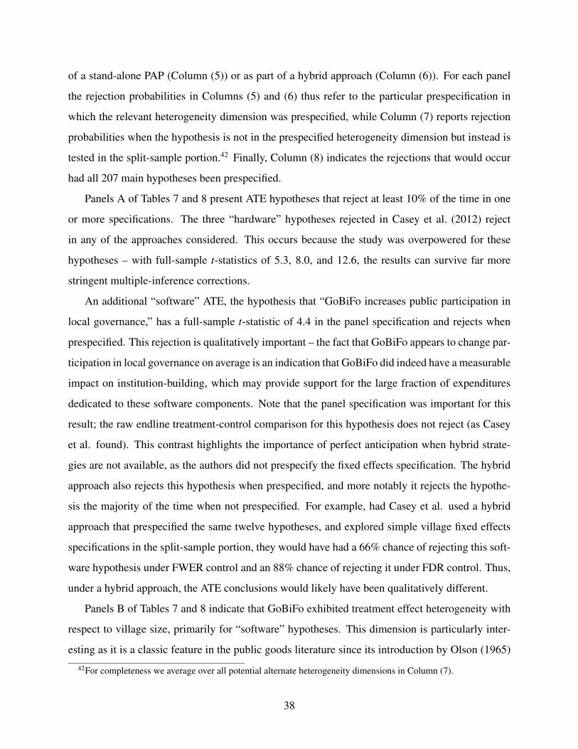
of a stand-alone PAP (Column (5)) or as part of a hybrid approach (Column (6)). For each panel

the rejection probabilities in Columns (5) and (6) thus refer to the particular prespecification in

which the relevant heterogeneity dimension was prespecified, while Column (7) reports rejection

probabilities when the hypothesis is not in the prespecified heterogeneity dimension but instead is

tested in the split-sample portion.42 Finally, Column (8) indicates the rejections that would occur

had all 207 main hypotheses been prespecified.

Panels A of Tables 7 and 8 present ATE hypotheses that reject at least 10% of the time in one

or more specifications. The three “hardware” hypotheses rejected in Casey et al. (2012) reject

in any of the approaches considered. This occurs because the study was overpowered for these

hypotheses – with full-sample t-statistics of 5.3, 8.0, and 12.6, the results can survive far more

stringent multiple-inference corrections.

An additional “software” ATE, the hypothesis that “GoBiFo increases public participation in

local governance,” has a full-sample t-statistic of 4.4 in the panel specification and rejects when

prespecified. This rejection is qualitatively important – the fact that GoBiFo appears to change par-

ticipation in local governance on average is an indication that GoBiFo did indeed have a measurable

impact on institution-building, which may provide support for the large fraction of expenditures

dedicated to these software components. Note that the panel specification was important for this

result; the raw endline treatment-control comparison for this hypothesis does not reject (as Casey

et al. found). This contrast highlights the importance of perfect anticipation when hybrid strate-

gies are not available, as the authors did not prespecify the fixed effects specification. The hybrid

approach also rejects this hypothesis when prespecified, and more notably it rejects the hypothe-

sis the majority of the time when not prespecified. For example, had Casey et al. used a hybrid

approach that prespecified the same twelve hypotheses, and explored simple village fixed effects

specifications in the split-sample portion, they would have had a 66% chance of rejecting this soft-

ware hypothesis under FWER control and an 88% chance of rejecting it under FDR control. Thus,

under a hybrid approach, the ATE conclusions would likely have been qualitatively different.

Panels B of Tables 7 and 8 indicate that GoBiFo exhibited treatment effect heterogeneity with

respect to village size, primarily for “software” hypotheses. This dimension is particularly inter-

esting as it is a classic feature in the public goods literature since its introduction by Olson (1965)

42For completeness we average over all potential alternate heterogeneity dimensions in Column (7).

38

– collective action becomes more difficult in larger groups. Furthermore, the authors explicitly

stratified on this dimension, guaranteeing that imbalance in treatment could not yield false hetero-

geneity results. Under 5% FWER control (Table 7), if the authors prespecified heterogeneity with

respect to village size they would have identified that in larger villages GoBiFo was less effective at

improving local project infrastructure and less effective at increasing access to information about

local governance. Under 5% FDR control (Table 8), if the authors prespecified heterogeneity with

respect to village size they would have found the same reduced effects on project infrastructure

and information, and also that in larger villages GoBiFo was less successful in increasing public

participation in local governance, and – perhaps surprisingly – that these decreases occurred even

though GoBiFo motivated more collective action and contributions to public goods. Column (5)

indicates that this last effect would have been found under a PAP that only specified ATEs and

the village-size dimension and a hybrid that prespecified the same, but not under a PAP that ex-

haustively specified all candidate dimensions of heterogeneity. Moreover, if the hybrid approach

were utilized with FDR control, the authors would have had a 52% chance of concluding that in

larger villages GoBiFo was also less effective at increasing inclusion and participation in commu-

nity planning and infrastructure if it were prespecified. This finding would not have been identified

under any of the PAPs considered.

Under the hybrid approach, the authors would have also likely concluded that village size was

a meaningful dimension of heterogeneity if they did not prespecify it. Under FWER control, there

is a 14-20% chance of concluding that larger villages were less effective at improving local project

infrastructure (depending on how many other hypotheses were prespecified) and a 19-24% chance

of concluding that larger villages were less effective at increasing access to information about

local governance. These chances become much larger under FDR control. Using a hybrid that did

not specify heterogeneity with respect to village size with the FDR correction, the authors would

have had a 51-58% chance of identifying that larger villages were less effective at improving local

project infrastructure, a 50-57% chance of identifying that larger villages were less effective at

increasing access to information, and a 48-59% chance of identifying that larger villages were less

effective at increasing participation in local governance, along with smaller chances on the other

two hypotheses that could have rejected if prespecified. Broadly, we conclude that GoBiFo had

meaningful treatment heterogeneity with respect to village size, and a researcher interested in this

39

dimension would have been able to identify about 4.5 differences under the hybrid approach (if

prespecified and using the FDR correction) and about 1.6 differences under the hybrid approach

if they had failed to prespecify this dimension. Thus, we conclude that using a hybrid approach

on the GoBiFo evaluation would have led to qualitatively different conclusions about the effects

of GoBiFo on institution building. Moreover, it would have expanded upon Olson’s insights on

the importance of the number of stakeholders by establishing that the number of stakeholders also

matters for the effectiveness of institution building around public good provision.

Panels C of Tables 7 and 8 document that there also appears to be meaningful heterogeneity

with respect to the baseline presence of an extractive chief on “software” outcomes. The presence

of an extractive chief is a signal on the local institutional environment. Theoretically, we might

anticipate an extractive chief to have two possible effects on GoBiFo provision. On the one hand,

an extractive chief may be more successful in diverting GoBiFo to his own purposes, weakening

institution building and negatively affecting both hardware and software outcomes (e.g., Ostrom

1996; Dayton-Johnson 2003). On the other hand, baseline levels of institutional quality and public

good provision may be lower under an extractive regime, which may amplify the impacts of GoB-

iFo. Quantitatively, we find that had the authors prespecified ATEs and heterogeneity with respect

to an extractive chief, they would have identified that GoBiFo was more effective in increasing

trust when an extractive chief was present (under both FWER and FDR control). Had they used

a hybrid they would have found this result under either FWER or FDR control if they prespeci-

fied it, and even when not prespecified they would have found it with 18-27% probability under

FWER control or with 69-74% probability under FDR control. Moreover, if they used a hybrid

approach and prespecified this dimension, they would also have identified with 92% probability

(under FDR control) that when there is an extractive chief, GoBiFo is less effective at improving

project infrastructure. This latter result could only have been found under a hybrid approach.

Panels D of Tables 7 and 8 document that GoBiFo was also differentially effective in Bombali

villages, at least on “hardware” outcomes. There may be contextual reasons to anticipate these ef-

fects, or one may have anticipated these effects due to differences in the sampling frame (sampled

Bombali villages are larger than non-Bombali villages). Once again, the benefits of the hybrid

approach are larger under FDR control, as are the number of rejections. However, absent a theoret-

ical lens to interpret this heterogeneity, we simply note that the ultimate conclusions of an analysis

40

on GoBiFo would have documented important heterogeneity in its effectiveness. This is perhaps

unsurprising given the implementation heterogeneity inherent to CDD programs, but nevertheless

of clear interest to program implementers.

Taking these results together, we conclude that GoBiFo affected all three hardware hypotheses,

as Casey et al. (2012) found. However, it also led to the software effect of increasing local partic-

ipation in public governance. Furthermore, there was important heterogeneity related to GoBiFo:

it was more effective in producing software outcomes in smaller villages and in villages with an

extractive chief at baseline. Discovering any of the software results in a PAP depends crucially on

which PAP was written. When using a hybrid approach, in contrast, at least some of the software

effects would have been found with very high probability. Our analysis of weighted rejections also

found that while the exhaustive PAP is attractive in terms of overall numbers of rejections, it is not

always the most effective in terms of rejections of any specific hypothesis.

6 Conclusions and Recommendations

Preanalysis plans have emerged as a powerful tool to control false discoveries, and, in doing so,

encourage scientific replicability. PAPs are not costless, however – researchers must correctly

anticipate the full menu of tests to be run without access to any data. This paper develops a split-

sample approach that allows researchers to learn from a portion of the data before finalizing an

analysis plan. We suggest several optimized ways to learn from a portion of the data, including

optimal sample splits, switching to one-sided tests, and thresholds for passing hypotheses. When

researchers can write down a preanalysis plan which includes all false hypotheses (so that they

need not learn from the data), and when the researchers’ objective function is to maximize the

expected number of rejections, preanalysis plans outperform the split-sample approach. However,

the optimized split-sample approach provides about 90% of the power of the pure PAP, so that they

may be preferred in cases where the researcher is unable to fully anticipate all tests that are to be

run in advance, either because she will learn about some tests to run from patterns in the data or

because the cost of her time is too high to fully develop a perfectly anticipatory PAP.

When hypotheses appear heterogeneous to a researcher ex ante, either in terms of prior beliefs

or intrinsic interest, a hybrid approach that prespecifies some hypotheses and searches through the

41

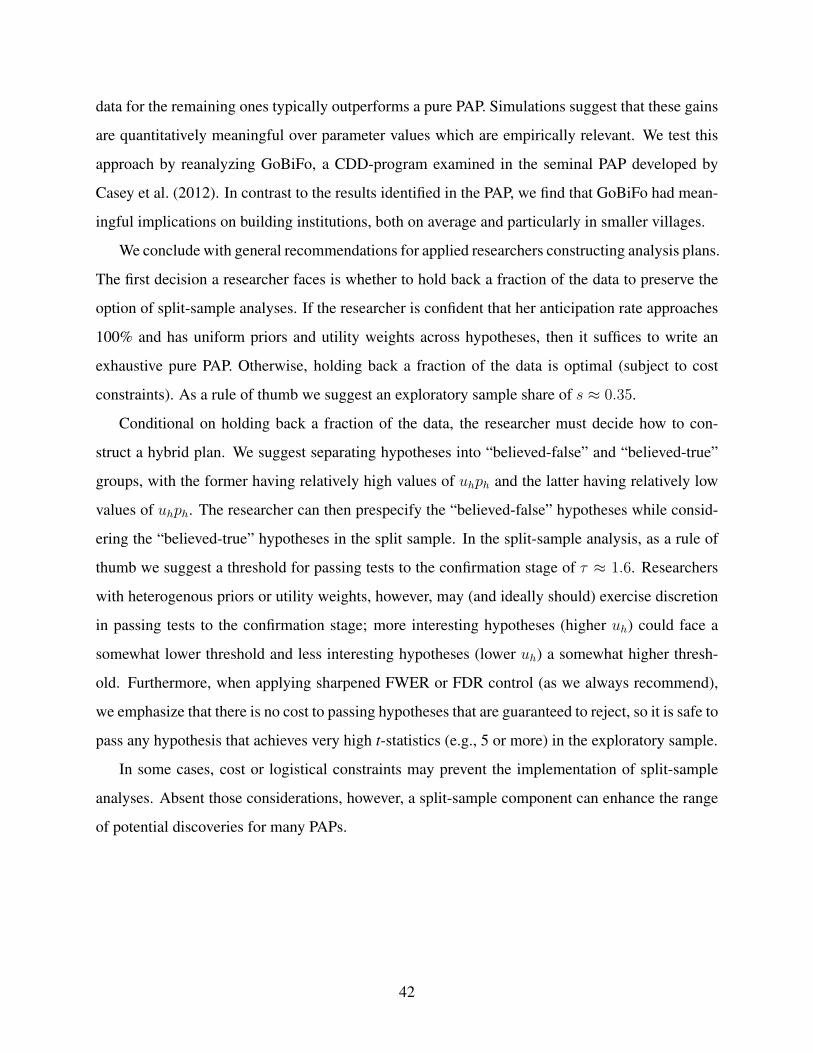
data for the remaining ones typically outperforms a pure PAP. Simulations suggest that these gains

are quantitatively meaningful over parameter values which are empirically relevant. We test this

approach by reanalyzing GoBiFo, a CDD-program examined in the seminal PAP developed by

Casey et al. (2012). In contrast to the results identified in the PAP, we find that GoBiFo had mean-

ingful implications on building institutions, both on average and particularly in smaller villages.

We conclude with general recommendations for applied researchers constructing analysis plans.

The first decision a researcher faces is whether to hold back a fraction of the data to preserve the

option of split-sample analyses. If the researcher is confident that her anticipation rate approaches

100% and has uniform priors and utility weights across hypotheses, then it suffices to write an

exhaustive pure PAP. Otherwise, holding back a fraction of the data is optimal (subject to cost

constraints). As a rule of thumb we suggest an exploratory sample share of s ≈ 0.35.

Conditional on holding back a fraction of the data, the researcher must decide how to con-

struct a hybrid plan. We suggest separating hypotheses into “believed-false” and “believed-true”

groups, with the former having relatively high values of uhph and the latter having relatively low

values of uhph. The researcher can then prespecify the “believed-false” hypotheses while consid-

ering the “believed-true” hypotheses in the split sample. In the split-sample analysis, as a rule of

thumb we suggest a threshold for passing tests to the confirmation stage of τ ≈ 1.6. Researchers

with heterogenous priors or utility weights, however, may (and ideally should) exercise discretion

in passing tests to the confirmation stage; more interesting hypotheses (higher uh) could face a

somewhat lower threshold and less interesting hypotheses (lower uh) a somewhat higher thresh-

old. Furthermore, when applying sharpened FWER or FDR control (as we always recommend),

we emphasize that there is no cost to passing hypotheses that are guaranteed to reject, so it is safe to

pass any hypothesis that achieves very high t-statistics (e.g., 5 or more) in the exploratory sample.

In some cases, cost or logistical constraints may prevent the implementation of split-sample

analyses. Absent those considerations, however, a split-sample component can enhance the range

of potential discoveries for many PAPs.

42

7 References

References

Alesina, A., Baqir, R., and Easterly, W. (1999). Public goods and ethnic divisions. Quarterly

Journal of Economics, 114:1234–84.

Anderson, M. L. (2008). Multiple inference and gender differences in the effects of early interven-

tion: A reevaluation of the abecedarian, perry preschool, and early training projects. Journal of

the American Statistical Association, 103(484):1481–1495.

Benjamini, Y., Krieger, A. M., and Yekutieli, D. (2006). Adaptive linear step-up procedures that

control the false discovery rate. Biometrika, 93(3):491–507.

Card, D., DellaVigna, S., and Malmendier, U. (2011). The Role of Theory in Field Experiments.

Journal of Economic Perspectives, 25(3):39–62.

Casey, K., Glennerster, R., and Miguel, E. (2012). Reshaping Institutions: Evidence on Aid Im-

pacts Using a Preanalysis Plan. The Quarterly Journal of Economics, 127(4):1755–1812.

Coffman, L. C. and Niederle, M. (2015). Pre-analysis Plans Have Limited Upside, Especially

Where Replications Are Feasible. Journal of Economic Perspectives, 29(3):81–98.

Dayton-Johnson, J. (2003). Small-holders and water resources: A review essay on the economics

of locally-managed irrigation. Oxford Development Studies, 31(3):315–339.

De Angelis, C., Drazen, J., Frizelle, F., Haug, C., Hoey, J., Horton, R., Kotzin, S., Laine, C.,

Marusic, A., Overbeke, A. J. P., Schroeder, T., Sox, H., and Van Der Weyden, M. (2004). Clinical

Trial Registration: A Statement from the International Committee of Medical Journal Editors.

Easterly, W. and Levine, R. (1997). Africa’s growth tragedy: Policies and ethnic division. Quar-

terly Journal of Economics, 112(4):1203–1250.

Fafchamps, M. and Labonne, J. (2017). Using Split Samples to Improve Inference about Causal

Effects. Working Paper, Stanford University.

43

Franco, A., Malhotra, N., and Simonovits, G. (2014). Publication bias in the social sciences:

Unlocking the file drawer. Science, 345(6203):1502–1505.

Gerber, A. and Malhotra, N. (2008). Do Statistical Reporting Standards Affect What Is Published?

Publication Bias in Two Leading Political Science Journals. Quarterly Journal of Political

Science, 3(3):313–326.

Horton, R. and Smith, R. (1999). Time to register randomised trials. BMJ, 319(7214):865–866.

Kling, J. R., Liebman, J. B., and Katz, L. F. (2007). Experimental analysis of neighborhood effects.

Econometrica, 75(1):83–119.

Larson, S. C. (1931). The shrinkage of the coefficient of multiple correlation. Journal of Educa-

tional Psychology, 22(1):45–55.

Ludwig, J., Kling, J. R., and Mullainathan, S. (2011). Mechanism Experiments and Policy Evalu-

ations. Journal of Economic Perspectives, 25(3):17–38.

Miguel, E., Camerer, C., Casey, K., Cohen, J., Esterling, K. M., Gerber, A., Glennerster, R., Green,

D. P., Humphreys, M., Imbens, G., Laitin, D., Madon, T., Nelson, L., Nosek, B. A., Petersen,

M., Sedlmayr, R., Simmons, J. P., Simonsohn, U., and Laan, M. V. d. (2014). Promoting Trans-

parency in Social Science Research. Science, 343(6166):30–31.

Miguel, E. and Gugerty, M. K. (2005). Ethnic diversity, social sanctions, and public goods in

kenya. Journal of Public Economics, 89(11-12):2325–2368.

Neumark, D. (2001). The employment effects of minimum wages: Evidence from a prespecified

research design the employment effects of minimum wages. Industrial Relations: A Journal of

Economy and Society, 40(1):121–144.

O’Brien, P. C. (1984). Procedures for comparing samples with multiple endpoints. Biometrics,

40(4):1079–1087.

Olken, B. A. (2015). Promises and Perils of Pre-analysis Plans. Journal of Economic Perspectives,

29(3):61–80.

44

Olson, M. (1965). The Logic of Collective Action: Public Goods and the Theory of Groups.

Harvard Economic Studies. Harvard University Press, 124 edition.

Ostrom, E. (1996). Incentives, rules of the game, and development. In Bruno, M. and Pleskovic,

B., editors, Proceedings of the Annual Bank Conference on Africa 1995, pages 207–234, Wash-

ington, D.C.

Ostrom, E. (2009). A general framework for analyzing sustainability of socio-ecological systems.

Science, 325:419–422.

Romano, J. P. and Wolf, M. (2005). Stepwise Multiple Testing as Formalized Data Snooping.

Econometrica, 73(4):1237–1282.

Simes, R. J. (1986). Publication bias: the case for an international registry of clinical trials. Journal

of Clinical Oncology, 4(10):1529–1541.

Snee, R. D. (1977). Validation of Regression Models: Methods and Examples. Technometrics,

19(4):415–428.

Sterling, T. D. (1959). Publication Decisions and their Possible Effects on Inferences Drawn

from Tests of Significance—or Vice Versa. Journal of the American Statistical Association,

54(285):30–34.

Stone, M. (1974). Cross-Validatory Choice and Assessment of Statistical Predictions. Journal of

the Royal Statistical Society. Series B (Methodological), 36(2):111–147.

Yong, E. (2012). Replication studies: Bad copy. Nature, 485(7398):298–300.

Figures and Tables

45

Figure 1: Optimal Exploratory Sample Share by Pass-on Threshold

0.1

.2.3

.4.5

.6O

ptim

al e

xplo

rato

ry sa

mpl

e sh

are

(s)

0 .5 1 1.5 2Exploratory sample t−statistic threshold for passing tests (τ)

Notes: H = 20 hypotheses tested or explored.

Figure 2: PAP and Split-Sample Power

0.2

.4.6

.8A

vera

ge p

ower

0.2

.4.6

.8A

vera

ge p

ower

.2 .3 .4Average effect size (µ)

Full Sample PAP Optimized Split SampleSplit Sample, τ = 0.2 Split Sample, τ = 1.0Balanced Split Sample

Notes: Exploratory share s = 0.15. See Table 1 for values of total hypotheses,

average effect size, and share false.

46

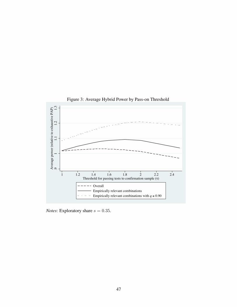
Figure 3: Average Hybrid Power by Pass-on Threshold

.91

1.1

1.2

1.3

Ave

rage

pow

er (r

elat

ive

to e

xhau

stive

PA

P)

1 1.2 1.4 1.6 1.8 2 2.2 2.4Threshold for passing tests to confirmation sample (τ)

OverallEmpirically relevant combinationsEmpirically relevant combinations with q ≥ 0.90

Notes: Exploratory share s = 0.35.

47

Figure 4: Distribution of Relative Power of Hybrid Plan

0.1

.2.3

Frac

tion

.8 1 1.2 1.4 1.6Power ratio of hybrid plan to exhaustive PAP

A. All parameter combinations

0.0

5.1

.15

Frac

tion

.8 1 1.2 1.4 1.6Power ratio of hybrid plan to exhaustive PAP

B. More empirically relevant parameter combinations

0.1

.2.3

.4Fr

actio

n

.8 1 1.2 1.4 1.6Power ratio of hybrid plan to exhaustive PAP, weighted

C. All parameter combinations0

.05

.1.1

5Fr

actio

n

.8 1 1.2 1.4 1.6Power ratio of hybrid plan to exhaustive PAP, weighted

D. More empirically relevant parameter combinations

0.1

.2.3

.4Fr

actio

n

0 1 2 3 4 5 6 7 8Power ratio of hybrid plan to PAP with believed−false hypotheses

E. All parameter combinations

0.0

5.1

.15

.2.2

5Fr

actio

n

1 2 3 4 5Power ratio of hybrid plan to PAP with believed−false hypotheses

F. More empirically relevant parameter combinations

Notes: Threshold for passing tests to confirmation sample is fixed at τ = 1.6; exploratory sample share is fixed at

s = 0.35.

48

Figure 5: Weighted Rejections in GoBiFo

.4.6

.81

1.2

Rela

tive

pow

er

1 2 3 4 5Weight

Restricted PAP Hybrid PAP

D. Extractive chief, 5% FDR

.8.9

11.

11.

2Re

lativ

e po

wer

1 2 3 4 5Weight

Restricted PAP Hybrid PAP

B. Number of households, 5% FDR

.6.7

.8.9

11.

1Re

lativ

e po

wer

1 2 3 4 5Weight

Restricted PAP Hybrid PAP

C. Extractive chief, 5% FWER

.75

.8.8

5.9

.95

Rela

tive

pow

er

1 2 3 4 5Weight

Restricted PAP Hybrid PAP

A. Number of households, 5% FWER

Notes: Power is normalized relative to an exhaustive PAP.

49

Table 1: Simulation Parameter Values

Parameter Values Mean Std DevP(false | believed false) (p ) 0.25, 0.50, 0.80, 1.00 0.64 0.33P(true | believed true) (q ) 0.80, 0.82, 0.84, …, 1.00 0.90 0.07Average effect size (μ) 0.2, 0.3, 0.4, 0.5 0.35 0.13Total hypotheses (H ) 10, 20, 50, 100 45 40.4Share believed false (H 1/H ) 0.10, 0.20, 0.50 0.27 0.21

Table 2: Average Power by Exploratory Sample Share for Hybrid Plan with Threshold τ = 1.6

Exploratory sample share (1) (2) (3) (4) (5)0.10 0.93 0.97 1.10 1.26 1.290.15 0.97 1.02 1.13 1.28 1.320.20 0.99 1.05 1.15 1.28 1.320.25 1.01 1.07 1.17 1.29 1.350.30 1.02 1.08 1.18 1.29 1.360.35 1.03 1.09 1.18 1.30 1.350.40 1.03 1.08 1.18 1.29 1.320.45 1.03 1.07 1.17 1.29 1.320.50 1.02 1.05 1.16 1.29 1.290.75 0.93 0.90 1.05 1.24 1.15Parameter restrictionsTotal hypotheses (H ) ≥ 50 ≥ 50 ≥ 50 = 100Share believed false (H 1/H ) ≤ 0.20 ≤ 0.20 ≤ 0.20 = 0.10Avg effect size (μ) ≤ 0.3 ≤ 0.3 ≤ 0.3 = 0.2P(true | believed true) (q ) ≥ 0.90 ≥ 0.96 ≥ 0.96

Combinations 21,120 3,520 1,920 720 30Notes: Each cell reports, for a given exploratory sample share, the average power ratio of a hybrid plan to an exhaustive PAP. The hybrid plan has a fixed threshold for passing tests to the confirmation sample of τ = 1.6. Column maximums are in bold.

50

Table 3: Determinants of Optimal Threshold for Passing Tests to Confirmation Sample

Dependent variable:(1) (2) (3)

P(true | believed true) (q ) 0.66 0.76 0.75(60.5) (35.3) (25.7)

Avg effect size (μ) -0.37 -0.34 -0.32(-34.5) (-15.6) (-10.8)

P(false | believed false) (p ) 0.26 0.36 0.40(23.8) (16.8) (13.5)

Total hypotheses (H ) 0.33 0.11 0.11(30.3) (5.3) (3.8)

Share believed false (H 1/H ) 0.06 0.05 0.03(5.3) (2.4) (1.2)

Parameter restrictionsTotal hypotheses (H ) ≥ 50 ≥ 50Share believed false (H 1/H ) ≤ 0.20 ≤ 0.20Avg effect size (μ) ≤ 0.3 ≤ 0.3P(true | believed true) (q ) ≥ 0.90

R 2 0.75 0.84 0.84N (combinations) 2,112 352 192Notes: In all regressions the dependent variable is the optimal threshold for passing tests to the confirmation sample. Parentheses contain t -statistics. The exploratory sample share is set to s = 0.35 in all cases.

Optimal threshold for passing tests (τ )

51

Table 4: Determinants of Hybrid Plan Power (Relative to Exhaustive PAP)

Dependent variable:(1) (2) (3)

P(true | believed true) (q ) 0.54 0.74 0.64(38.2) (34.6) (23.6)

Avg effect size (μ) -0.44 -0.42 -0.59(-31.4) (-19.5) (-21.8)

P(false | believed false) (p ) 0.24 0.32 0.31(17.2) (15.2) (11.2)

Total hypotheses (H ) 0.10 0.02 0.04(7.4) (1.1) (1.5)

Share believed false (H 1/H ) 0.13 0.13 0.05(9.1) (6.2) (1.8)

Parameter restrictionsTotal hypotheses (H ) ≥ 50 ≥ 50Share believed false (H 1/H ) ≤ 0.20 ≤ 0.20Avg effect size (μ) ≤ 0.3 ≤ 0.3P(true | believed true) (q ) ≥ 0.90

R 2 0.58 0.84 0.86N (combinations) 2,112 352 192Notes: In all regressions the dependent variable is the power ratio of a hybrid plan relative to an exhaustive PAP. Parentheses contain t -statistics. The exploratory sample share is set to s = 0.35 in all cases.

Relative hybrid plan power

52

Table 5: GoBiFo Hypotheses and Baseline Covariates

A. "Hardware" Hypotheses t -statFWERp -val

1 GoBiFo project implementation 12.8 0.0002 Participation in GoBiFo improves local project infrastructure 5.2 0.0003 Participation in GoBiFo improves general economic welfare 8.0 0.000

B. "Software" Hypotheses4 Participation in GoBiFo increases collective action and contributions to 0.3 0.9805 GoBiFo increases inclusion and participation in community planning and

implementation, especially for poor and vulnerable groups; GoBiFo norms spill over into other types of community decisions, making them more

0.1 0.980

6 GoBiFo changes local systems of authority, including the roles and public perceptions of traditional leaders (chiefs) versus local elected government

1.5 0.664

7 Participation in GoBiFo increases trust 0.9 0.9138 Participation in GoBiFo builds and strengthens community networks 0.8 0.9139 Participation in GoBiFo increases access to information about local 1.0 0.913

10 GoBiFo increases public participation in local governance 2.0 0.31511 By increasing trust, GoBiFo reduces crime and conflict in the community 0.2 0.98012 GoBiFo changes political and social attitudes, making individuals more

liberal toward women, more accepting of other ethnic groups and 1.0 0.913

C. Candidate Heterogeneity Dimensions 1 Number of households*2 Distance to the road*3 Ethnolinguistic fractionalization4 Baseline presence of an extractive chief5 War exposure6 Anyone in the village owns/has owned a slave7 Average education8 Bombali district*

Notes: * indicates dimension of explicit stratification. Values of t -statistics and FWER p -values are taken from Table 2 of Casey et al. (2012).

53

Table 6: Rejections in GoBiFo under different analysis plans

5% FWER 10% FWER 5% FDRPrespecification Method (1) (2) (3)

PAP 3 3 3Hybrid 5.3 5.9 8.4

(1.0) (1.1) (1.6)

PAP 3 3 3Hybrid 5.5 6.1 8.7

(1.1) (1.2) (1.7)

PAP 4 4 4Hybrid 5.5 6.0 8.3

(0.9) (1.0) (1.5)

PAP 6 7 8Hybrid 7.1 7.4 11.0

(0.6) (0.8) (1.2)

PAP 5 5 5Hybrid 6.2 6.5 9.1

(0.8) (0.9) (1.5)

PAP 6 6 7Hybrid 6.5 6.7 9.2

(0.6) (0.8) (1.1)

PAP 4 4 4Hybrid 5.4 5.8 7.7

(0.8) (1.0) (1.4)

PAP 4 4 4Hybrid 5.4 5.8 7.8

(0.8) (1.0) (1.4)

PAP 4 4 4Hybrid 5.4 5.8 7.8

(0.8) (1.0) (1.4)

PAP 4 4 4Hybrid 5.4 5.8 7.8

(0.8) (1.0) (1.4)

PAP 4 4 4Hybrid 5.4 5.8 7.8

(0.9) (1.0) (1.4)

PAP 8 9 10

PAP 5 5 9All heterogeneity and all candidate dependent variables in PAP*Notes : Each cell presents the total rejections for a given prespecification plan and multiplicity adjustment. Columns represent multiplicity adjustments while rows represent alternative prespecifications. Parentheses contain standard deviations of results across random sample splits. * indicates that only rejections of hypothesis indices are reported.

Distance to road + all ATE

Anyone owned slaves + all ATE

Years of education + all ATE

War exposure + all ATE

Ethnolinguistic fractionalization + all ATE

All heterogeneity in PAP

Bombali district + all ATE

As written in Casey et al. (2012)

Hardware only

All ATE

Number of households + all ATE

Extractive chief + all ATE

54

Table 7: Rejections in GoBiFo under different analysis plans and 5% FWER

PrespecificationAnalysis

Full sample

t -statistic

All heterogeneity dimensions

All dependent variables

Method PAP Hybrid PAP Hybrid PAP PAP PAPPre-

specifiedSplit

sampleHypothesis (1) (2) (3) (4) (5) (6) (7) (8) (9)

GoBiFo implementation Endline 12.57 1.00 1.00 1.00 1.00 1.00 1.00 1.00 1.00GoBiFo improves local project infrastructure Endline 5.27 1.00 1.00 1.00 1.00 1.00 1.00 1.00 1.00

GoBiFo improves general economic welfare Endline 8.01 1.00 1.00 1.00 1.00 1.00 1.00 1.00 1.00

GoBiFo increases public participation in local governance Panel 4.42 0 0.66 0 0.69 1.00 1.00 1.00 1.00

GoBiFo improves local project infrastructure

Panel -3.79 0 0.17 0 0.20 1.00 1.00 0.14 1.00 0

GoBiFo increases collective action and contributions to public goods

Panel 2.68 0 0 0 0 0 0 0 0 0

GoBiFo increases inclusion and participation in community planning and implementation…

Panel -2.43 0 0 0 0 0 0 0 0 0

Participation in GoBiFo increases access to information about local governance

Panel -3.86 0 0.21 0 0.24 1.00 1.00 0.19 1.00 0

GoBiFo increases public participation in local governance Panel -3.17 0 0.01 0 0.01 0 0 0.00 0 0

PAP as written Hardware-only PAP

All ATEs + one heterogeneity dimension

Hybrid

A. Average treatment effects

B. Heterogeneous treatment effects, by village size

55

PrespecificationAnalysis

Full sample

t -statistic

All heterogeneity dimensions

All dependent variables

Method PAP Hybrid PAP Hybrid PAP PAP PAPPre-

specifiedSplit

sampleHypothesis (1) (2) (3) (4) (5) (6) (7) (8) (9)

GoBiFo improves local project infrastructure

Panel -2.56 0 0 0 0 0 0 0 0 0

Participation in GoBiFo increases trust Panel 3.66 0.222 0.00 0.266 1.00 1.00 0.18 0.00 0 0

GoBiFo improves local project infrastructure Endline -3.91 0 0.19 0 0.21 1.00 1.00 0.16 1.00 0

GoBiFo implementation Panel -2.97 0 0 0 0 0 0 0 0 0GoBiFo improves general economic welfare Panel 4.76 0 0.83 0 0.83 1.00 1.00 0.79 1.00 1.00

C. Heterogeneous treatment effects, by presence of an extractive chief

D. Heterogeneous treatment effects, by Bombali district

Notes: Each cell reports the frequency of rejections for a given hypothesis under each potential prespecification. PAPs are deterministic while hybrid results are probabilistic based on random sample splits. FWER controlled at 5%. Column (6) indicates the power if the prespecification is all ATEs plus the relevant heterogeneity dimension, while Column (7) indicates the power if the prespecification is all ATEs plus a different heterogeneity dimension (averaged across all candidate heterogeneity dimensions).

PAP as written Hardware-only PAP

All ATEs + one heterogeneity dimension

Hybrid

56

Table 8: Rejections in GoBiFo under different analysis plans and 5% FDR

PrespecificationAnalysis

Full sample

t -statistic

All heterogeneity dimensions

All dependent variables

Method PAP Hybrid PAP Hybrid PAP PAP PAPPre-

specifiedSplit

sampleHypothesis (1) (2) (3) (4) (5) (6) (7) (8) (9)

GoBiFo implementation Endline 12.57 1.00 1.00 1.00 1.00 1.00 1.00 1.00 1.00GoBiFo improves local project infrastructure Endline 5.27 1.00 1.00 1.00 1.00 1.00 1.00 1.00 1.00

GoBiFo improves general economic welfare Endline 8.01 1.00 1.00 1.00 1.00 1.00 1.00 1.00 1.00

GoBiFo increases public participation in local governance Panel 4.42 0 0.88 0 0.88 1.00 1.00 1.00 1.00

GoBiFo improves local project infrastructure

Panel -3.79 0 0.57 0 0.58 1.00 1.00 0.51 1.00 1.00

GoBiFo increases collective action and contributions to public goods

Panel 2.68 0 0.1 0 0.13 1.00 1.00 0.05 0 0

GoBiFo increases inclusion and participation in community planning and implementation…

Panel -2.43 0 0.01 0 0.02 0 0.52 0.00 0 0

Participation in GoBiFo increases access to information about local governance

Panel -3.86 0 0.55 0 0.57 1.00 1.00 0.50 1.00 1.00

GoBiFo increases public participation in local governance Panel -3.17 0 0.57 0 0.59 1.00 1.00 0.48 1.00 0

PAP as written Hardware-only PAP

All ATEs + one heterogeneity dimension

Hybrid

A. Average treatment effects

B. Heterogeneous treatment effects, by village size

57

PrespecificationAnalysis

Full sample

t -statistic

All heterogeneity dimensions

All dependent variables

Method PAP Hybrid PAP Hybrid PAP PAP PAPPre-

specifiedSplit

sampleHypothesis (1) (2) (3) (4) (5) (6) (7) (8) (9)

GoBiFo improves local project infrastructure

Panel -2.56 0 0.03 0 0.06 0 0.92 0.01 0 0

Participation in GoBiFo increases trust Panel 3.66 0 0.73 0 0.74 1.00 1.00 0.69 1.00 1.00

GoBiFo improves local project infrastructure Endline -3.91 0 0.58 0 0.60 1.00 1.00 0.56 1.00 1.00

GoBiFo implementation Panel -2.97 0 0.36 0 0.41 1.00 1.00 0.24 0 0GoBiFo improves general economic welfare Panel 4.76 0 0.91 0 0.91 1.00 1.00 0.91 1.00 1.00

C. Heterogeneous treatment effects, by presence of an extractive chief

D. Heterogeneous treatment effects, by Bombali district

Notes: Each cell reports the frequency of rejections for a given hypothesis under each potential prespecification. PAPs are deterministic while hybrid results are probabilistic based on random sample splits. FDR controlled at 5%. Column (6) indicates the power if the prespecification is all ATEs plus the relevant heterogeneity dimension, while Column (7) indicates the power if the prespecification is all ATEs plus a different heterogeneity dimension (averaged across all candidate heterogeneity dimensions).

PAP as written Hardware-only PAP

All ATEs + one heterogeneity dimension

Hybrid

58

AppendixNot For Print Publication

A1 Optimal pure PAP

Suppose the researcher has access to H hypotheses which may be true or false, and false hypothe-

ses are characterized by a data generating process where βh = b > 0. If priors over the hypotheses

being false and weights over rejecting individual hypotheses are uniform, we prove that the optimal

PAP would include all of them.

Suppose one would prespecify H−1 hypotheses and was considering prespecifying one more.

One would be willing to prespecify all H hypotheses if

P(th > t α2H|βh = b) > (H − 1)

[P(tk > t α

2(H−1)|βk = b)− P(tk > t α

2H|βk = b)

]Since P(th > τ |βh = b) = P(tk > τ |βk = b) ∀ k, h with uniform hypotheses, this implies that

HP(th > t α2H|βh = b)− (H − 1)P(th > t α

2(H−1)|βh = b) > 0 (10)

The left side equals 0 when b = 0. Therefore, if we show that the derivative of Equation (10)

is increasing with respect to b ∀ H , we can conclude that for b > 0 additional hypotheses should

be included in the PAP. Letting P(th > t α2H|βh = b) = (1−Φ(t α

2H− b)) and t α

2H= Φ−1(1− α

2H),

where Φ represents the normal CDF, the derivative of Equation (10) wrt b is given by

Hφ(t α2H− b)− (H − 1)φ(t α

2(H−1)− b) > 0

where φ is the normal PDF. If we rearrange and take logs this condition becomes

ln(H)− 0.5 t2α2H

+ b t α2H> ln(H − 1)− 0.5 t2

α2(H−1)

+ b t α2(H−1)

(11)

This reveals that the value of including hypotheses is increasing in b if ln(H)−0.5 t2α2H

+ b t α2H

is increasing in H . To verify this, we differentiate the left side of Equation (11) with respect to H

and observe that we should include hypotheses if

1

H+b( α

2H2 )

φ(t α2H

)>

(t α2H

)( α2H2 )

φ(t α2H

)

59

Now note that

1− Φ(x) ≤ φ(x)

xsince x(1− Φ(x)) =

∫ ∞x

xφ(u)du ≤∫ ∞x

uφ(u)du = −φ(u)|∞x = φ(x)

Thus we see that 1H

=α

2H2

1−Φ(t α2H

)≥

(t α2H

)( α2H2 )

φ(t α2H

), so it is sufficient to show that

1

H+b( α

2H2 )

φ(t α2H

)>

1

H

which clearly holds for b > 0 and all H . Thus, a researcher facing a data generating process

with uniform hypotheses and b > 0 will want to prespecify all hypotheses.

A2 Optimal Exploratory Share and Pass-on Thresholds

Suppose we have H hypotheses, H − 1 of which are true, and there are N total observations. We

are interested in the power on the remaining false hypothesis, for which we assume β = b. If

we use a Bonferroni correction to control FWER, assign fraction s of the data in the exploratory

sample, and pass on all hypotheses where |teh| > τ , then the power function for our false hypothesis

can be represented as

H∑k1=0

(H

k1

)(Φ(−τ) +

(1− Φ(τ)

))k1·(Φ(τ)− Φ(−τ)

)H−k1·[Φ(−τ − b

√sN/4) · Φ(−tα/k1+1 − b

√(1− s)N/4)

+(1− Φ(τ − b

√sN/4)

)·(1− Φ(tα/k1+1 − b

√(1− s)N/4)

)]where tα/k1+1 is the t critical value for a test of size α

k1+1. Taking the first order condition with

respect to s, one can find an approximate closed form for the optimal exploratory share. Let m(.)

represent the Mills ratio; the optimal exploratory share is approximately a function of the expected

Mills ratios in the two stages, given by√1− s∗s∗

≈ Ek1[ m(τ − b

√s∗N/4)

m(tα/k1+1 − b√

(1− s∗)N/4)

]Since m′(.) < 0, the optimal exploratory share is increasing in the τ threshold.

60

A3 Optimal Type I Error Allocation

To motivate the optimal allocation of type I error, consider a simple case in which a researcher

tests two hypotheses. The conventional allocation of type I error splits it evenly between the two

hypotheses, with each receiving α = 0.025. If a researcher were confident that first hypothesis was

false but skeptical that second one was false, she might test only the first one in the confirmation

sample, implicitly assigning α = 0.05 type I error to it and α = 0 type I error to the second one.

If she were only somewhat more confident about the first hypothesis rejecting than the second,

however, then the optimal allocation of type I error to each test would not be binary in nature. She

might, for example, allocate α = 0.04 type I error to the first hypothesis and α = 0.01 type I error

to the second hypothesis.

To solve for the optimal allocation of type I error across tests we return to the Agnostic Evalu-

ation Problem. Letting Rh represent an indicator for hypothesis h rejecting, the problem is

maxH∑h=1

Rh

If the researcher knows the sampling distributions of the test statistics, which we assume are

t-statistics in this case, then this problem becomes

maxαh

H∑h=1

Ft(F−1t (1− αh)− E[tch]),

where Ft represents the t cumulative distribution function and E[tch] represents the expectation of

hypothesis h’s t-statistic in the confirmation sample. Solving this problem yields the first order

condition (FOC)

ft(F−1t (1− αh)− E[tch])

ft(F−1t (1− αh))

=ft(F

−1t (1− αh′)− E[tch′ ])

ft(F−1t (1− αh′))

∀ h, h′,

where ft represents the t probability density function. The numerator in the FOC represents the

marginal return, in terms of rejection probability, to relaxing the t critical value for hypothesis

h. The denominator in the FOC represents the marginal change in the size of the test, αh, from

relaxing the t critical value for hypothesis h. The FOC thus reveals that type I error should first be

allocated to the test with the highest return per unit of type I error, and at the optimum the return

to allocating type I error should be equal across all tests with positive type I error allocations.

61

In practice the researcher does not know E[tch] – if she did there would be no need to run the

experiment. The obvious solution is to use the exploratory sample coefficient estimate, βeh, to

estimate E[tch] = βeh/σch (where σch is a consistent estimator of βch’s standard error). This estimate

of E[tch] is consistent, but in any finite sample it suffers from a regression-to-the-mean problem:

Large values of βeh tend to be large both because the true βh is non-zero and because there has

been a shock in the same direction as the coefficient. Using the raw estimate βeh thus tends to over

allocate type I error to hypotheses with large exploratory sample t-statistics and under allocate

it to hypotheses with modest exploratory sample t-statistics. This suggests applying a shrinkage

estimator to the exploratory sample coefficient estimates.

The shrinkage estimator we consider is the Empirical Bayes estimator. This estimator applies

Bayes Theorem:

P(βh|βeh) =P(βeh|βh) · P(βh)

P(βeh).

Using the empirical distribution of the coefficients from the exploratory sample, βej , and apply-

ing the law of iterated expectations we estimate:

P(βh|βeh) =P(βeh|βh) ·H−1∑Hj=1 P(βeh|βej ) ·H−1

=P(βeh|βh)∑Hj=1 P(βeh|βej )

.

Note that we only evaluate P(βh|βeh) for values of βh corresponding to points of support in the

empirical distribution of βej , and the denominator is a constant that ensures the posterior proba-

bilities sum to one.43 To understand the estimator’s operation, consider the largest βej , βemax. The

posterior for βmax is centered below βemax because βemax is the upper bound of the support for any

posterior. Other coefficient estimates βej “pull down” E[βmax], with each posterior point of support

βej receiving weight P(βemax|βmax = βej ). Thus the estimator “shrinks” larger coefficients towards

the empirical mean of the coefficients. With the posterior distribution P(βh|βeh) it is trivial to esti-

mate E[tch] and compute the FOCs. In practice we assign type I error based on the expectation of

the FOC (using the posterior distribution) rather than the FOC evaluated at the estimate of E[tch].44

In summary, by solving the Agnostic Evaluation Problem and applying a shrinkage estimator,

we can allocate type I error to hypotheses in incremental amounts using information from the

exploratory sample. In our simulations, when expected t-statistics are modest or the share of

43To compute P(βeh|βh) we appeal to the Central Limit Theorem and assume a normal distribution for βeh.44This seems desirable since the FOC is not linear in E[tch].

62

hypotheses that are false is low, this optimized type I error allocation results in modest increases in

power over a rule that passes all hypotheses with t-statistics exceeding a threshold τ . However, the

power differences are small when comparing against “loose” thresholds that pass on most tests.

A4 Proof of Proposition 1

For the proposition, it suffices to demonstrate that there is a hybrid plan that uses split-sample

search for at least one hypothesis and that is superior to the optimal pure PAP. Suppose there exists

an optimal pure PAP with an internal solution, that is, that ∃ Hp ⊂ H s.t. h ∈ Hp are prespecified

and h /∈ Hp are not. For each hypothesis h, define εh by

εh =∑j∈Hp

ujpj

[P(tj > t α

2|Hp||βj = b)− P(tj > t α

2(|Hp|+1)|βj = b)

]−uhphP(th > t α

2(|Hp+1|)|βh = b)

so that hypotheses with εh < 0 would be included in the optimal pure PAP and those with εh > 0

would not. Finally, suppose that there exists a “marginal” hypothesis, a, such that for any δ > 0:

0 < εa < δ (12)

By definition, the researcher is, in the limit, indifferent between including or omitting hypothe-

sis a from the pure PAP. Now consider adding hypothesis a to the split-sample portion of a hybrid

plan that prespecifies Hp. Analyzing hypothesis a in the exploratory sample (and conditionally

testing it in the confirmation sample) leads to power gains over the optimal PAP if

uapaP(tca > t α|Hp|+1

|βa = b)P(tea > τ |βa = b)

>[paP(|tea| > τ |βa = b) + (1− pa)2P(t > τ)

](13)

·∑j∈Hp

ujpj

[P(tj > t α

2|Hp||βj = b)− P(tj > t α

2(|Hp|+1)|βj = b)

]Or, using the definition of εh, if

uapaP(tca > t α|Hp|+1

|βa = b)P(tea > τ |βa = b)

>[paP(|tea| > τ |βa = b) + (1− pa)2P(t > τ)

]·[uapaP(ta > t α

2(|Hp|+1)|βa = b) + εa

]63

Simplifying, we have

uapa

[ P(tca > t α|Hp|+1

|βa = b)P(tea > τ |βa = b)

paP(|tea| > τ |βa = b) + (1− pa)2P(t > τ)− P(ta > t α

2(|Hp|+1)|βa = b)

]> εa (14)

Let Φ(.), Φ(.), and φ(.) represent the CDF, upper-tail CDF, and PDF, respectively, of the stan-

dard normal distribution. Let σcb = 2/√

(1− s)N , σeb = 2/√sN , and σb = 2/

√N . Then we can

rewrite Equation (14) as

uapa

[ Φ(t α|Hp|+1

− b/σcb) · Φ(τ − b/σeb)

pa(Φ(−τ − b/σeb) + Φ(τ − b/σeb)) + 2(1− pa)Φ(τ)− Φ(t α

2(|Hp|+1)− b/σb)

]> εa

Since we can bound εa arbitrarily close to zero, it suffices to show that

Φ(τ − b/σeb)pa(Φ(−τ − b/σeb) + Φ(τ − b/σeb)) + 2(1− pa)Φ(τ)

>Φ(t α

2(|Hp|+1)− b/σb)

Φ(t α|Hp|+1

− b/σcb)

Now note that the left-hand side achieves a minimum when pa = 1, so we can prove the

proposition by proving that

Φ(τ − b/σeb)Φ(−τ − b/σeb) + Φ(τ − b/σeb)

=1

Φ(τ + b/σeb)/Φ(τ − b/σeb) + 1>

Φ(t α2(|Hp|+1)

− b/σb)

Φ(t α|Hp|+1

− b/σcb)(15)

Choose s = s∗ such that (b/σb − b/σc∗b ) < (t α2(|Hp|+1)

− t α|Hp|+1

). ThusΦ(t α

2(|Hp|+1)−b/σb)

Φ(t α|Hp|+1

−b/σc∗b )= η,

where η < 1. Applying L’Hopital’s rule to the left-hand side of Equation (15) we see that

limτ→∞

1

Φ(τ + b/σe∗b )/Φ(τ − b/σe∗b ) + 1= lim

τ→∞

1

φ(τ + b/σe∗b )/φ(τ − b/σe∗b ) + 1

= limτ→∞

1

e−2τb/σe∗b + 1= 1

Thus we can choose τ = τ ∗ such that η < 1Φ(τ∗+b/σe∗b )/Φ(τ∗−b/σe∗b )+1

< 1.45 These choices of s∗

and τ ∗ satisfy Equation (15), so a hybrid plan that prespecifies Hp and considers hypothesis a in

the split-sample portion using a sufficiently low value of s and a sufficiently high value of τ will

outperform the optimal pure PAP in expectation.

45For completeness, note that we may choose δ in Equation (12) to be less than ( 1Φ(τ∗+b/σe∗b )/Φ(τ∗−b/σe∗b )+1

− η) ·

uapa · Φ(t α|Hp|+1

− b/σc∗b ).

64

In practice there may not be sufficient density of uhph to guarantee the existence of a truly

marginal hypothesis with εh arbitrarily close to zero, in which case the proposition might not

hold. When considering sharpened FWER or FDR control, however, we can substantially relax

the marginal hypothesis condition in Equation (12). The intuition is straightforward – with FWER

or FDR sharpening, a hypothesis that rejects after multiplicity adjustments does not “consume”

any type I error, because we can be virtually certain that the rejection is not false. Setting a

high threshold, τ , for passing tests to the confirmation sample ensures that tests will reject at the

confirmation stage with probability approaching one and impose no multiple testing penalty on the

prespecified hypotheses. There is thus near-zero cost to considering the marginal hypothesis in the

split-sample when using a high value of τ .46 As long as there exists some probability of a large

effect size, then a hybrid plan with a high τ threshold that considers the marginal hypothesis in the

split-sample portion will outperform the pure PAP that omits the marginal hypothesis. For example,

suppose that N = 500 and that the optimal pure PAP includes |Hp| = 100 hypotheses. If there

is a 1 in 100,000 chance of an effect size of 0.3 (0.8) standard deviations in a panel specification

(endline comparison), then a hybrid plan that considers the marginal hypothesis, a, using s = 0.2

and τ = 7 will outperform the optimal pure PAP as long as the average utility weight uh for

hypotheses inHp is no more than ten times larger than ua.47

46With FWER or FDR sharpening, the term that premultiplies the summation in Equation (13) changes from the

probability that hypothesis a passes to the confirmation stage to the probability that hypothesis a passes to the confir-

mation stage and fails to reject. For large τ this probability approaches zero.47For this calculation we assume that the prior distribution on βa is weakly decreasing in b. We also make the

worst-case assumptions that ph ≈ 1 for all hypotheses in Hp and that βh ≈ t α2|Hp|

. These assumptions are extremely

conservative. Stata code to calculate bounds for different parameter values is available upon request.

65

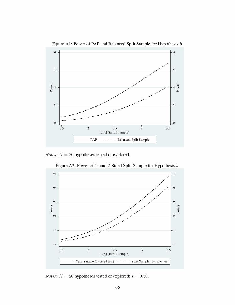
Figure A1: Power of PAP and Balanced Split Sample for Hypothesis h

0.2

.4.6

.8Po

wer

0.2

.4.6

.8Po

wer

1.5 2 2.5 3 3.5E[th] (in full sample)

PAP Balanced Split Sample

Notes: H = 20 hypotheses tested or explored.

Figure A2: Power of 1- and 2-Sided Split Sample for Hypothesis h

0.1

.2.3

.4.5

Pow

er

0.1

.2.3

.4.5

Pow

er

1.5 2 2.5 3 3.5E[th] (in full sample)

Split Sample (1−sided test) Split Sample (2−sided test)

Notes: H = 20 hypotheses tested or explored; s = 0.50.

66

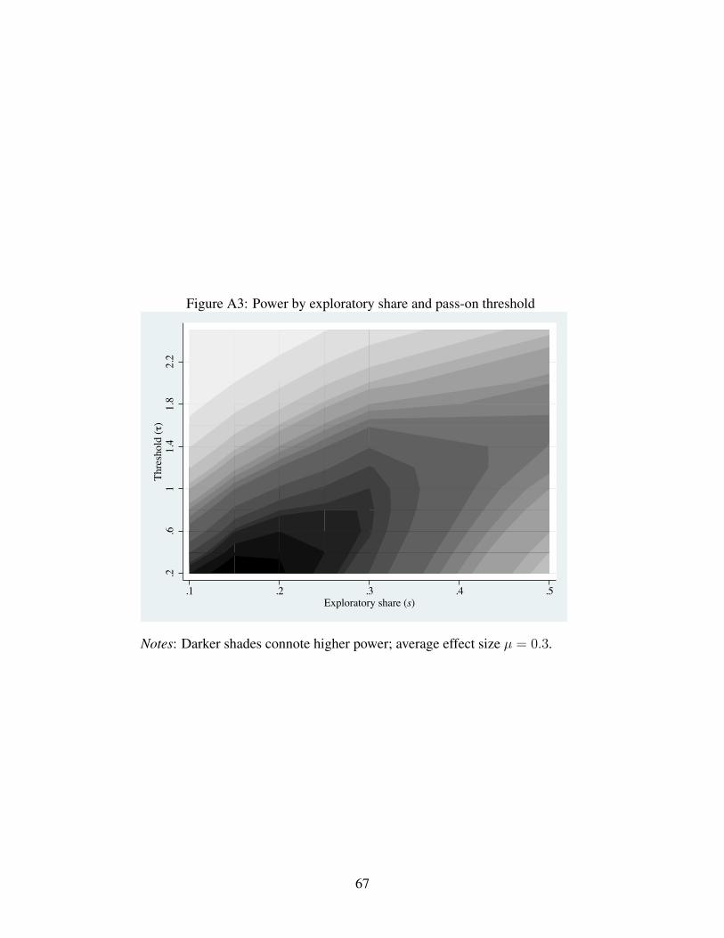
Figure A3: Power by exploratory share and pass-on threshold

.2.6

11.

41.

82.

2Th

resh

old

(τ)

.1 .2 .3 .4 .5Exploratory share (s)

Notes: Darker shades connote higher power; average effect size µ = 0.3.

67

Table A1: Average Power by Exploratory Sample Share (FWER)

Exploratory sample share (1) (2) (3) (4) (5) (6)

0.20 1.006 1.054 1.142 1.000 1.053 1.1480.25 1.021 1.070 1.154 1.017 1.070 1.1600.30 1.027 1.074 1.158 1.029 1.082 1.1720.35 1.030 1.072 1.156 1.031 1.080 1.1710.40 1.028 1.061 1.149 1.030 1.072 1.1650.45 1.021 1.044 1.139 1.025 1.058 1.1570.50 1.010 1.021 1.123 1.017 1.037 1.144

0.20 0.994 1.050 1.154 0.979 1.042 1.1630.25 1.013 1.074 1.173 1.001 1.069 1.1840.30 1.023 1.083 1.177 1.014 1.081 1.1900.35 1.030 1.087 1.183 1.025 1.093 1.2020.40 1.031 1.081 1.180 1.028 1.093 1.2020.45 1.027 1.069 1.174 1.028 1.086 1.2000.50 1.020 1.050 1.159 1.023 1.071 1.189Parameter restrictionsTotal hypotheses (H ) ≥ 50 ≥ 50 ≥ 50 ≥ 50Share believed false (H 1/H ) ≤ 0.20 ≤ 0.20 ≤ 0.20 ≤ 0.20Avg effect size (μ) ≤ 0.3 ≤ 0.3 ≤ 0.3 ≤ 0.3P(true | believed true) (q ) ≥ 0.90 ≥ 0.90

Combinations 14,784 2,464 1,344 14,784 2,464 1,344

Panel A: τ = 1.4 Panel B: τ = 1.5

Panel C: τ = 1.6 Panel D: τ = 1.8

Notes: Each cell reports, for a given exploratory sample share, the average power ratio of a hybrid plan to an exhaustive PAP, controlling FWER. The hybrid plan has a fixed threshold τ for passing tests to the confirmation sample; τ varies by panel. Column maximums are in bold.

68

Table A2: Average Power by Exploratory Sample Share (FDR)Exploratory sample share (1) (2) (3) (4) (5) (6)

0.20 0.977 1.006 1.125 0.970 1.003 1.1330.25 0.996 1.030 1.144 0.991 1.029 1.1540.30 1.007 1.046 1.154 1.004 1.048 1.1650.35 1.014 1.050 1.153 1.012 1.055 1.1660.40 1.016 1.050 1.153 1.016 1.057 1.1690.45 1.015 1.045 1.151 1.016 1.054 1.1680.50 1.009 1.029 1.138 1.011 1.041 1.157

0.20 0.963 0.999 1.139 0.946 0.987 1.1490.25 0.985 1.027 1.162 0.970 1.017 1.1730.30 0.999 1.048 1.175 0.986 1.041 1.1880.35 1.009 1.057 1.177 0.999 1.053 1.1930.40 1.014 1.062 1.183 1.007 1.064 1.2030.45 1.016 1.062 1.183 1.011 1.067 1.2050.50 1.012 1.051 1.175 1.010 1.062 1.201Parameter restrictionsTotal hypotheses (H ) ≥ 50 ≥ 50 ≥ 50 ≥ 50Share believed false (H 1/H ) ≤ 0.20 ≤ 0.20 ≤ 0.20 ≤ 0.20Avg effect size (μ) ≤ 0.3 ≤ 0.3 ≤ 0.3 ≤ 0.3P(true | believed true) (q ) ≥ 0.90 ≥ 0.90

Combinations 14,784 2,464 1,344 14,784 2,464 1,344

Panel A: τ = 1.4 Panel B: τ = 1.5

Panel C: τ = 1.6 Panel D: τ = 1.8

Notes: Each cell reports, for a given exploratory sample share, the average power ratio of a hybrid plan to an exhaustive PAP, controlling FDR. The hybrid plan has a fixed threshold τ for passing tests to the confirmation sample; τ varies by panel. Column maximums are in bold.

69