
SPIRE Observers’ Manual -...
101
SPIRE Observers’ Manual HERSCHEL-DOC-0798, version 2.4, June 7, 2011
Transcript of SPIRE Observers’ Manual -...
SPIRE Observers’ Manual
HERSCHEL-DOC-0798, version 2.4, June 7, 2011

2
SPIRE Observers’ Manual
Version 2.4, June 7, 2011
This document is based on inputs from the SPIRE Consortium and the SPIRE InstrumentControl Centre.
Document custodian: Ivan Valtchanov, Herschel Science Centre.

Contents
1 Introduction 7
1.1 The Observatory . . . . . . . . . . . . . . . . . . . . . . . . . . . . . . . . . . 7
1.2 Purpose and Structure of Document . . . . . . . . . . . . . . . . . . . . . . . 7
1.3 Acknowledgements . . . . . . . . . . . . . . . . . . . . . . . . . . . . . . . . . 8
1.4 Changes to Document . . . . . . . . . . . . . . . . . . . . . . . . . . . . . . . 8
1.4.1 Changes in version 2.4 (OT2 call) . . . . . . . . . . . . . . . . . . . . 8
1.4.2 Changes in version 2.3 (GT2 call) . . . . . . . . . . . . . . . . . . . . 8
1.4.3 Changes in version 2.2 . . . . . . . . . . . . . . . . . . . . . . . . . . . 9
1.4.4 Changes in version 2.1 . . . . . . . . . . . . . . . . . . . . . . . . . . . 9
1.4.5 Changes in version 2.0 . . . . . . . . . . . . . . . . . . . . . . . . . . . 10
1.5 List of Acronyms . . . . . . . . . . . . . . . . . . . . . . . . . . . . . . . . . . 11
2 The SPIRE Instrument 13
2.1 Instrument Overview . . . . . . . . . . . . . . . . . . . . . . . . . . . . . . . . 13
2.2 Photometer design . . . . . . . . . . . . . . . . . . . . . . . . . . . . . . . . . 14
2.2.1 Optics and layout . . . . . . . . . . . . . . . . . . . . . . . . . . . . . 14
2.2.2 Beam steering mirror (BSM) . . . . . . . . . . . . . . . . . . . . . . . 15
2.2.3 Filters and passbands . . . . . . . . . . . . . . . . . . . . . . . . . . . 15
2.2.4 Photometer calibration source (PCAL) . . . . . . . . . . . . . . . . . . 16
2.2.5 Photometer detector arrays . . . . . . . . . . . . . . . . . . . . . . . . 16
2.3 Spectrometer design . . . . . . . . . . . . . . . . . . . . . . . . . . . . . . . . 17
2.3.1 Fourier-Transform Spectrometer Concept and Mode of Operation . . . 17
2.3.2 Spectrometer optics and layout . . . . . . . . . . . . . . . . . . . . . . 18
2.3.3 Spectrometer calibration source (SCAL) . . . . . . . . . . . . . . . . . 19
2.3.4 Filters and passbands . . . . . . . . . . . . . . . . . . . . . . . . . . . 20
2.3.5 Spectrometer detector arrays . . . . . . . . . . . . . . . . . . . . . . . 20
2.4 Common Instrument Parts . . . . . . . . . . . . . . . . . . . . . . . . . . . . 21
3

4 CONTENTS
2.4.1 Basic bolometer operations . . . . . . . . . . . . . . . . . . . . . . . . 21
2.4.2 3He cooler and thermal strap system . . . . . . . . . . . . . . . . . . . 23
2.4.3 Warm electronics . . . . . . . . . . . . . . . . . . . . . . . . . . . . . . 24
3 Observing with SPIRE 25
3.1 Introduction . . . . . . . . . . . . . . . . . . . . . . . . . . . . . . . . . . . . . 25
3.2 SPIRE Photometer AOT . . . . . . . . . . . . . . . . . . . . . . . . . . . . . 26
3.2.1 Large Map . . . . . . . . . . . . . . . . . . . . . . . . . . . . . . . . . 26
3.2.2 Small Map . . . . . . . . . . . . . . . . . . . . . . . . . . . . . . . . . 32
3.2.3 Dithering of SPIRE scan maps . . . . . . . . . . . . . . . . . . . . . . 35
3.2.4 Point Source . . . . . . . . . . . . . . . . . . . . . . . . . . . . . . . . 37
3.3 SPIRE Spectrometer AOT . . . . . . . . . . . . . . . . . . . . . . . . . . . . . 41
3.3.1 Spectral Resolution . . . . . . . . . . . . . . . . . . . . . . . . . . . . . 42
3.3.2 Pointing Modes . . . . . . . . . . . . . . . . . . . . . . . . . . . . . . . 44
3.3.3 Image Sampling . . . . . . . . . . . . . . . . . . . . . . . . . . . . . . 46
3.3.4 User input parameters for all Spectrometer AOTs. . . . . . . . . . . . 47
3.3.5 Spectrometer dark sky observations . . . . . . . . . . . . . . . . . . . 50
3.3.6 Considerations when preparing FTS observations . . . . . . . . . . . . 51
3.4 Using HSpot to prepare AOR . . . . . . . . . . . . . . . . . . . . . . . . . . . 51
4 SPIRE in-flight performance 53
4.1 Photometer performance . . . . . . . . . . . . . . . . . . . . . . . . . . . . . . 53
4.1.1 Beam profiles . . . . . . . . . . . . . . . . . . . . . . . . . . . . . . . . 53
4.1.2 Sensitivity . . . . . . . . . . . . . . . . . . . . . . . . . . . . . . . . . . 54
4.1.3 Observing overheads . . . . . . . . . . . . . . . . . . . . . . . . . . . . 57
4.1.4 Some HSpot examples . . . . . . . . . . . . . . . . . . . . . . . . . . . 57
4.2 Spectrometer . . . . . . . . . . . . . . . . . . . . . . . . . . . . . . . . . . . . 58
4.2.1 Spectral range, line shape and spectral resolution . . . . . . . . . . . . 58
4.2.2 Wavelength scale accuracy . . . . . . . . . . . . . . . . . . . . . . . . . 60
4.2.3 Beam profiles . . . . . . . . . . . . . . . . . . . . . . . . . . . . . . . . 60
4.2.4 Sensitivity . . . . . . . . . . . . . . . . . . . . . . . . . . . . . . . . . . 61
4.2.5 Some HSpot Examples . . . . . . . . . . . . . . . . . . . . . . . . . . . 63

CONTENTS 5
5 Flux Density Calibration 65
5.1 Calibration sources and models . . . . . . . . . . . . . . . . . . . . . . . . . . 65
5.1.1 Neptune and Uranus angular sizes and solid angles . . . . . . . . . . . 65
5.1.2 Neptune and Uranus models . . . . . . . . . . . . . . . . . . . . . . . 66
5.1.3 Mars models . . . . . . . . . . . . . . . . . . . . . . . . . . . . . . . . 66
5.1.4 Asteroid models . . . . . . . . . . . . . . . . . . . . . . . . . . . . . . 67
5.1.5 Stellar calibrators . . . . . . . . . . . . . . . . . . . . . . . . . . . . . 68
5.2 Photometer flux calibration scheme . . . . . . . . . . . . . . . . . . . . . . . . 69
5.2.1 Photometer Relative Spectral Response Function . . . . . . . . . . . . 69
5.2.2 Calibration flux densities . . . . . . . . . . . . . . . . . . . . . . . . . 70
5.2.3 Response of a SPIRE bolometer to incident power . . . . . . . . . . . 72
5.2.4 Conversion of RSRF-weighted flux density to monochromatic flux density 74
5.2.5 Colour correction . . . . . . . . . . . . . . . . . . . . . . . . . . . . . . 75
5.2.6 Conversion of in-beam flux density to surface brightness . . . . . . . . 76
5.2.7 Photometer beam maps and areas . . . . . . . . . . . . . . . . . . . . 77
5.2.8 Computed conversion factors for SPIRE . . . . . . . . . . . . . . . . . 80
5.2.9 Conversion from point source to extended source calibration . . . . . . 82
5.2.10 Photometer calibration accuracy . . . . . . . . . . . . . . . . . . . . . 84
5.2.11 A note on point source extraction from SPIRE Level-2 maps . . . . . 85
5.2.12 Summary . . . . . . . . . . . . . . . . . . . . . . . . . . . . . . . . . . 87
5.2.13 Future plans for photometer flux calibration . . . . . . . . . . . . . . . 87
5.3 Spectrometer flux calibration . . . . . . . . . . . . . . . . . . . . . . . . . . . 88
5.3.1 Spectrometer beam properties . . . . . . . . . . . . . . . . . . . . . . . 90
5.3.2 Extended sources and spectral mapping . . . . . . . . . . . . . . . . . 90
5.3.3 Dynamic range and interferogram clipping . . . . . . . . . . . . . . . . 91
5.3.4 Bright source mode . . . . . . . . . . . . . . . . . . . . . . . . . . . . . 92
5.3.5 Spectrometer calibration accuracy . . . . . . . . . . . . . . . . . . . . 94
5.3.6 Summary . . . . . . . . . . . . . . . . . . . . . . . . . . . . . . . . . . 94
6 SPIRE data products 95
Bibliography 99

6 CONTENTS
Chapter 1
Introduction
1.1 The Observatory
The Herschel Space Observatory (Pilbratt et al., 2010) is the fourth cornerstone mission inESA’s science programme. Herschel was successfully launched on 14th May 2009 from Kourou,French Guiana and with its passively cooled 3.5 m diameter primary mirror is currently thelargest telescope in space. Herschel is in an extended orbit around of the L2, the secondLagrangian point of the system Sun-Earth. The three on-board instruments: the HeterodyneInstrument for Far Infrared (HIFI, De Graauw et al. 2010), the Photodetector Array Cameraand Spectrometer (PACS, Poglitch et al. 2010) and the Spectral and Photometric ImagingReceiver (SPIRE, Griffin et al. 2010) had their first light after the thermal stabilisation periodof two months ended with the cryo-cover opening. The commissioning and performanceverification phases of the instruments had started much earlier than the cryo-cover opening.These phases are very important in order to confirm that the instruments were not damagedduring the launch and to validate that they will achieve their scientific objectives, namelyto perform photometry and spectroscopy observations in the infrared and the far-infrareddomains, from∼ 60 to∼ 672 µm. This spectral domain covers the cold and the dusty universe:from dust-enshrouded galaxies at cosmological distances down to scales of stellar formation,planetary system bodies and our own solar system objects. The operational lifetime of theobservatory, as dictated by the liquid helium boil-off, is estimated to be about 3.5 years.
A high-level description of the Herschel Space Observatory is given in Pilbratt et al. (2010);more details are given in the Herschel Observers’ Manual. The first scientific results arepresented in the special volume 518 of Astronomy & Astrophysics journal. Information withlatest news, announcement of opportunities for observing programmes, documentation, toolsetc is provided in the Herschel Science Centre web portal (http://herschel.esac.esa.int).
1.2 Purpose and Structure of Document
The purpose of this manual is to provide relevant information about the SPIRE instrumentin order to help the astronomers to prepare and execute scientific observations with it.
The structure of the document is as follows: first we describe the instrument (Chapter 2),followed by the description of the available observing modes and how to use them (Chapter 3).
7
8 CHAPTER 1. INTRODUCTION
In-flight performance of SPIRE is presented in Chapter 4. The flux calibration scheme isexplained in Chapter 5. The SPIRE data products are presented in Chapter 6. The list ofreferences is given in the last chapter.
1.3 Acknowledgements
This manual is provided by the Herschel Science Centre, based on inputs by the SPIREConsortium and by the SPIRE instrument team.
1.4 Changes to Document
1.4.1 Changes in version 2.4 (OT2 call)
• Updates to Chapter 3 (Observing with SPIRE):
– Added a subsection about the SPIRE Spectrometer dark sky observations (Sec-tion 3.3.5).
– Added a subsection about important considerations to be taken into account whenplanning FTS observations (Section 3.3.6).
• Updates to Chapter 4 (SPIRE in-flight performance):
– Updated the in-flight Spectrometer sensitivities in Section 4.2.4.
– Weighted-average instrumental line shapes of unresolved lines for the two centraldetectors are shown in Figure 4.2.
• Updates to Chapter 5 (Flux density calibration):
– Photometer beam maps and areas (Section 5.2.7), updates to the text, no changesin the beam sizes and areas.
– Point source extraction from maps (Section 5.2.11), some updates to the text.
– Improvements to the text in Section 5.3.1 (Spectrometer beam properties).
– Updated the Spectrometer calibration accuracy, Section 5.3.5.
1.4.2 Changes in version 2.3 (GT2 call)
• Updated the information for the photometer beam profiles in Chapters 4 and 5.
• Updated Figure 5.5 – now the photometer RSRF is given as a function of the frequency,the wavelength scale is only given for information.
• Minor updates to the numbers in Section 5.2.9.
• Updates to the pixelisation corrections for SPIRE maps in Section 5.2.11.

1.4. CHANGES TO DOCUMENT 9
1.4.3 Changes in version 2.2
• Chapter 3, added a short section about “dithering” for scan maps.
• Chapter 4
– Updated the information for the photometer and spectrometer beam profiles.
– Updated the sensitivity for the spectrometer, now we confirm that the noise scalesdown as expected for at least 100 repetitions.
– Bright source mode for spectrometer is now taken in consideration for the spec-trometer sensitivity summary.
• Chapter 5. This is a major revision of this chapter. Briefly the main updates are:
– The flux calibration schemes for both the photometer and the spectrometer aredescribed in detail.
– Photometer flux calibration is now Neptune based and all the quoted numbers fordifferent conversions are quoted for this case.
– Photometer beam characterisation is further improved and presented as a functionof map pixel size.
– Photometer conversion from point source to extended source is explained in detail.
– The overall photometer calibration accuracy is described.
– Practical note on point source extraction from SPIRE level-2 maps is also given.
– The spectrometer flux calibration scheme is presented with more details and prac-tical considerations.
– Updated spectrometer RSRF, based on Uranus.
– Spectrometer beams are presented as function of frequency: both the FWHM aswell as the beam solid angle for an extended emission.
– Spectrometer bright-source mode is explained, with recommendation on when touse this mode.
• Chapter 6 is now describing only the SPIRE data products while providing referencesto the pipeline documentation.
• Updates to the list of references.
1.4.4 Changes in version 2.1
• A swap of the spectrometer array label for the bright source settings in Section 5.3.4.The correct numbers per array are (175, 55) Jy for (SSW, SLW).

10 CHAPTER 1. INTRODUCTION
1.4.5 Changes in version 2.0
This document is a major update of the pre-launch version 1.2 for the “Announcement ofOpportunity for Key Projects”. Some of the key changes are listed below:
• Chapter 1, Introduction: minor changes to text
• Chapter 2, The SPIRE Instrument:
– Changes to Figure 2.2 with the correct sky position of the SPIRE Spectrometer.
– Added figures with photos of a bolometer, of the cooler, and of the detector arraymodule.
– Changes to the text to reflect the current in-flight numbers and conditions of thedifferent subsystems of SPIRE and to match the published papers on SPIRE.
• Chapter 3, Observing with SPIRE. There were major changes to this chapter to reflectthe in-flight observing modes.
– The Small Map mode based on 64-point jiggle pattern was replaced by a new scanmap mode with two small cross-scans.
– Real life examples of scan map and spectral mapping coverage.
– The information that was provided by the SPIRE instrument team for the releaseof each observing mode is incorporated in the relevant sections.
• Chapter 4, SPIRE in-flight performance. There were major updates to this chapter toreflect the in-flight performance of SPIRE.
• Chapter 5, Flux Density Calibration. This is a major update to the pre-flight “Calibra-tion” chapter. It presents the calibration framework for SPIRE. Note that it is still aninterim version, updates are to be released in the near future.
• Chapter 6, Pipeline and data products. This is a major update to the pre-flight chapterto reflect the actual systematic SPIRE data processing at the HSC.
• The Bibliography. Many new references were added.

1.5. LIST OF ACRONYMS 11
1.5 List of Acronyms
AOR Astronomical Observation RequestAOT Astronomical Observation TemplateBSM Beam Steering MirrorDCU Detector Control UnitDP Data ProcessingDPU Digital Processing UnitESA European Space AgencyFCU FPU Control UnitFIR Far Infrared RadiationFOV Field of ViewFPU Focal Plane UnitFTS Fourier-Transform SpectrometerHCSS Herschel Common Software SystemHIFI Heterodyne Instrument for the Far InfraredHIPE Herschel Interactive Processing EnvironmentHSC The Herschel Science Centre (based in ESAC, ESA, Spain)HSpot Herschel Observation Planning ToolIA Interactive AnalysisILT Instrument Level Test (i.e. ground tests of the instrument without the spacecraft)ISM Inter Stellar MediumJFET Junction Field-Effect TransistorNEP Noise-Equivalent PowerOPD Optical Path DifferencePACS Photodetector Array Camera and SpectrometerPCAL Photometer Calibration SourcePFM Proto-Flight Model of the instrumentPLW SPIRE Photometer Long (500 µm) Wavelength ArrayPMW SPIRE Photometer Medium (350 µm) Wavelength ArrayPSW SPIRE Photometer Short (250 µm) Wavelength ArrayPTC Photometer Thermal Control UnitRMS,rms Root Mean SquareRSRF Relative Spectral Response FunctionSCAL Spectrometer Calibration SourceSED Spectral Energy DistributionSLW SPIRE Long (316-672 µm) Wavelength Spectrometer ArraySMEC Spectrometer MechanismSNR, S/N Signal-to-Noise RatioSPG Standard Product GenerationSPIRE Spectral and Photometric Imaging REceiverSSW SPIRE Short (194-324 µm) Wavelength Spectrometer ArrayZPD Zero Path Difference

12 CHAPTER 1. INTRODUCTION

Chapter 2
The SPIRE Instrument
2.1 Instrument Overview
SPIRE consists of a three-band imaging photometer and an imaging Fourier Transform Spec-trometer (FTS). The photometer carries out broad-band photometry (λ/∆λ ≈ 3) in threespectral bands centred on approximately 250, 350 and 500 µm, and the FTS uses two over-lapping bands to cover 194-671 µm (447-1550 GHz).
Figure 2.1 shows a block diagram of the instrument. The SPIRE focal plane unit (FPU) isapproximately 700× 400× 400 mm in size and is supported from the 10 K Herschel opticalbench by thermally insulating mounts. It contains the optics, detector arrays (three for thephotometer, and two for the spectrometer), an internal 3He cooler to provide the requireddetector operating temperature of ∼ 0.3 K, filters, mechanisms, internal calibrators, andhousekeeping thermometers. It has three temperature stages: the Herschelcryostat providestemperatures of 4.5 K and 1.7 K via high thermal conductance straps to the instrument, andthe 3He cooler serves all five detector arrays.
Both the photometer and the FTS have cold pupil stops conjugate with the Herschel sec-ondary mirror, which is the telescope system pupil, defining a 3.29 m diameter used portionof the primary. Conical feedhorns (Chattopadhaya et al., 2003) provide a roughly Gaussianillumination of the pupil, with an edge taper of around 8 dB in the case of the photometer.The same 3He cooler design (Duband et al., 1998) is used in SPIRE and in the PACS instru-ment (Poglitch et al., 2010). It has two heater-controlled gas gap heat switches; thus one ofits main features is the absence of any moving parts. Liquid confinement in zero-g is achievedby a porous material that holds the liquid by capillary attraction. A Kevlar wire suspensionsystem supports the cooler during launch whilst minimising the parasitic heat load. Thecooler contains 6 STP litres of 3He, fits in a 200 × 100 × 100 mm envelope and has a massof ∼ 1.7 kg. Copper straps connect the 0.3-K stage to the five detector arrays, and are heldrigidly at various points by Kevlar support modules (Hargrave et al., 2006). The supports atthe entries to the 1.7-K boxes are also light-tight.
All five detector arrays use hexagonally close-packed feedhorn-coupled spider-web NeutronTransmutation Doped (NTD) bolometers (Turner et al., 2001). The bolometers are AC-biasedwith frequency adjustable between 50 and 200 Hz, avoiding 1/f noise from the cold JFETreadouts. There are three SPIRE warm electronics units: the Detector Control Unit (DCU)
13

14 CHAPTER 2. THE SPIRE INSTRUMENT
Figure 2.1: SPIRE instrument architecture
provides the bias and signal conditioning for the arrays and cold electronics, and demodulatesand digitises the detector signals; the FPU Control Unit (FCU) controls the cooler and themechanisms, and reads out all the FPU thermometers; and the Digital Processing Unit (DPU)runs the on-board software and interfaces with the spacecraft for commanding and telemetry.
A summary of the most important instrument characteristics is shown in Table 2.1 andthe operational parts of SPIRE are presented in the subsequent sections. A more detaileddescription of SPIRE can be found in Griffin et al. (2010).
SPIRE shares the Herschel focal plane with HIFI and PACS and it relative position withrespect to the other two instruments is shown in Figure 2.2.
2.2 Photometer design
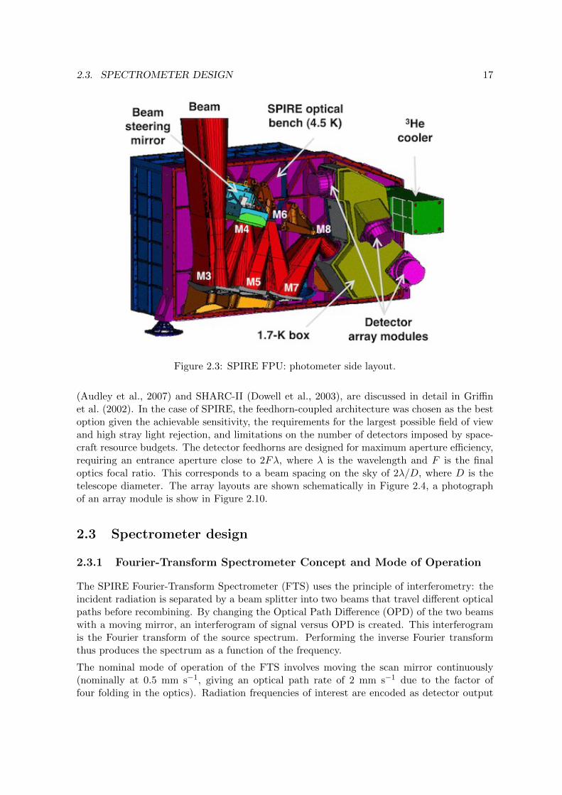
2.2.1 Optics and layout
The photometer opto-mechanical layout is shown in Figure 2.3. It is an all-reflective design(Dohlen et al. 2000) except for the dichroics used to direct the three bands onto the bolometerarrays, and the filters used to define the passbands (Ade et al. 2006). The input mirror M3,lying below the telescope focus, receives the f/8.7 telescope beam and forms an image of thesecondary at the flat beam steering mirror (BSM), M4. Mirror M5 converts the focal ratioto f/5 and provides an intermediate focus at M6, which re-images the M4 pupil to a coldstop. The input optics are common to the photometer and spectrometer and the separatespectrometer field of view is directed to the other side of the optical bench panel by a pick-offmirror close to M6. The 4.5-K optics are mounted on the SPIRE internal optical bench.

2.2. PHOTOMETER DESIGN 15
Table 2.1: SPIRE overall characteristics.
Sub-instrument Photometer Spectrometer
Array PSW PMW PLW SSW SLW
Band (µm) 250 350 500 194-313 303-671
Resolution (λ/∆λ) 3.3 3.4 2.5 ∼ 40− 1000 at 250 µm (variable)a
Unvignetted field of view 4′ × 8′ 2.0′ (diameter)
Beam FWHM size (arcsec)b 18.2 24.9 36.3 17-21 29-42
(a) – the unapodized spectral resolution can be low (∆σ = 0.83 cm−1), medium (∆σ = 0.24 cm−1) or
high (∆σ = 0.04 cm−1). See Section 4.2.1 for details.
(b) – The photometer beam FWHM are given for nominal SPIRE level-2 maps with pixel sizes (6,10,14)
arcsec, see Section 5.2.7. The FTS beam size depends on wavelength. See Section 5.3.1.
Mirrors M7, M8 and a subsequent mirror inside the 1.7-K box form a one-to-one optical relayto bring the M6 focal plane to the detectors. The 1.7-K enclosure also contains the threedetector arrays and two dichroic beam splitters to direct the same field of view onto thearrays so that it can be observed simultaneously in the three bands. The images in each bandare diffraction-limited over the 4’x8’ field of view.
2.2.2 Beam steering mirror (BSM)
The BSM (M4 in Figure 2.3) is located in the optical path before any subdivision of theincident radiation into photometer and spectrometer optical chains, and is used both forphotometer and FTS observations. For photometric observations the BSM is moved on apattern around the nominal position of the source. For the FTS, the BSM is moved on aspecific pattern to create intermediate or fully sampled spectral maps. It can chop up to ±2arcmin along the long axis of the Photometer’s 4× 8 arcmin field of view and simultaneouslychop in the orthogonal direction by up to 30 arcsec. This two-axis motion allows “jiggling”of the pointing to create fully sampled image of the sky. The nominal BSM chop frequencyfor the photometer is 1 Hz. For scanning observations the BSM is kept at its home position.
2.2.3 Filters and passbands
The photometric passbands are defined by quasi-optical edge filters (Ade et al. 2006) locatedat the instrument input, at the 1.7-K cold stop, and directly in front of the detector arrays,the reflection-transmission edges of the dichroics, and the cut-off wavelengths of the feedhornoutput waveguides. The filters also serve to minimise the thermal loads on the 1.7-K and0.3-K stages. The three bands are centred at approximately 250, 350 and 500 µm and theirrelative spectral response curves (RSRF) are given in much more detail in Section 5.2.1 (seeFigure 5.5).

16 CHAPTER 2. THE SPIRE INSTRUMENT
Figure 2.2: SPIRE location on sky with respect to the other two instruments sharing theHerschel focal plane. The centre of the SPIRE photometer is offset by ≈11 arcmin from thecentre of the highly curved focal surface of the Herschel telescope, shown by the large shadedcircle.
2.2.4 Photometer calibration source (PCAL)
PCAL is a thermal source used to provide a repeatable signal for the bolometers (Pisano etal., 2005). It operates as an inverse bolometer: applied electrical power heats up an emittingelement to a temperature of around 80 K, causing it to emit FIR radiation, which is seen bythe detectors. It is not designed to provide an absolute calibration of the system; this willbe done by observations of standard astronomical sources. The PCAL radiates through a 2.8mm hole in the centre of the BSM (occupying an area contained within the region of the pupilobscured by the hole in the primary). Although optimised for the photometer detectors, itcan also be viewed by the FTS arrays. PCAL is operated at regular intervals in-flight in orderto check the health and the responsivity of the arrays.
2.2.5 Photometer detector arrays
The three arrays contain 139 (250 µm), 88 (350 µm) and 43 (500 µm) detectors, each with itsown individual feedhorn. The feedhorn array layouts are shown schematically in Figure 2.4.The design features of the detectors and feedhorns are described in more detail in Section2.4.1.
The relative merits of feedhorn-coupled detectors, as used by SPIRE, and filled array de-tectors, which are used by PACS and some ground-based instruments such as SCUBA-2
2.3. SPECTROMETER DESIGN 17
Figure 2.3: SPIRE FPU: photometer side layout.
(Audley et al., 2007) and SHARC-II (Dowell et al., 2003), are discussed in detail in Griffinet al. (2002). In the case of SPIRE, the feedhorn-coupled architecture was chosen as the bestoption given the achievable sensitivity, the requirements for the largest possible field of viewand high stray light rejection, and limitations on the number of detectors imposed by space-craft resource budgets. The detector feedhorns are designed for maximum aperture efficiency,requiring an entrance aperture close to 2Fλ, where λ is the wavelength and F is the finaloptics focal ratio. This corresponds to a beam spacing on the sky of 2λ/D, where D is thetelescope diameter. The array layouts are shown schematically in Figure 2.4, a photographof an array module is show in Figure 2.10.
2.3 Spectrometer design
2.3.1 Fourier-Transform Spectrometer Concept and Mode of Operation
The SPIRE Fourier-Transform Spectrometer (FTS) uses the principle of interferometry: theincident radiation is separated by a beam splitter into two beams that travel different opticalpaths before recombining. By changing the Optical Path Difference (OPD) of the two beamswith a moving mirror, an interferogram of signal versus OPD is created. This interferogramis the Fourier transform of the source spectrum. Performing the inverse Fourier transformthus produces the spectrum as a function of the frequency.
The nominal mode of operation of the FTS involves moving the scan mirror continuously(nominally at 0.5 mm s−1, giving an optical path rate of 2 mm s−1 due to the factor offour folding in the optics). Radiation frequencies of interest are encoded as detector output

18 CHAPTER 2. THE SPIRE INSTRUMENT
Figure 2.4: A schematic view of the photometer bolometer arrays, the bolometer names arealso shown. Each circle represents a detector feedhorn. Those detectors centred on samesky positions are shaded in blue, the dead bolometers are shaded in grey. The 4 × 8 arcminunvignetted field of view of each array is delineated by a red dashed rectangle. The threearrays overlap on the sky as shown in the rightmost figure, where the PLW (500 µm), PMW(350 µm) and PSW (250 µm) are depicted by red, green and blue circles respectively. Thecircle sizes in the rightmost figure correspond to the FWHM of the beam. The spacecraftcoordinate system (Y,Z) is also shown.
electrical frequencies in the range 3-10 Hz. For an FTS, the resolution element is given by∆σ = 1/(2×OPDmax), where OPDmax is the maximum optical path difference of the scanmirror. The maximum mechanical scan length is 3.5 cm, equivalent to an OPDmax of 14 cm,thus the highest resolution available is ∆σ = 0.04 cm−1, which corresponds to ∆ν = 1.2 GHzresolution in frequency space. The number of independent samples in the final spectrum isset by the resolution, i.e. independent points in the spectrum are separated in wavenumberspace by ∆σ and this is constant throughout the whole wavelength range covered by the FTS.
2.3.2 Spectrometer optics and layout
The FTS (Swinyard et al., 2003; Dohlen et al., 2000) uses two broadband intensity beamsplitters in a Mach-Zehnder configuration which has spatially separated input and outputports. This configuration leads to a potential increase in efficiency from 50% to 100% incomparison with a Michelson interferometer. One input port views a 2.6 arcmin diameterfield of view on the sky and the other an on-board reference source (SCAL). Two bolometerarrays at the output ports cover overlapping bands of 194-313 µm (SSW) and 303-671 µm

2.3. SPECTROMETER DESIGN 19
(SLW). As with any FTS, each scan of the moving mirror produces an interferogram in whichthe spectrum of the entire band is encoded with the spectral resolution corresponding to themaximum mirror travel.
The FTS focal plane layout is shown in Figure 2.5. A single back-to-back scanning roof-top mirror serves both interferometer arms. It has a frictionless mechanism using doubleparallelogram linkage and flex pivots, and a Moire fringe sensing system. A filtering schemesimilar to the one used in the photometer restricts the passbands of the detector arrays atthe two ports, defining the two overlapping FTS bands.
Figure 2.5: SPIRE FPU: spectrometer side layout.
2.3.3 Spectrometer calibration source (SCAL)
A thermal source, the Spectrometer Calibrator (SCAL, Hargrave et al. 2006), is available asan input to the second FTS port to allow the background power from the telescope to benulled, thus reducing the dynamic range (because the central maximum of the interferogramis proportional to the difference of the power from the two input ports). SCAL is located atthe pupil image at the second input port to the FTS, and has two sources which can be usedto simulate different possible emissivities of the telescope: 2% and 4%.
The in-flight FTS calibration measurements of Vesta, Neptune and Uranus with SCAL offshowed that the signal at the peak of the interferogram is not saturated or at most only afew samples are saturated, which means that SCAL is not required to reduce the dynamicrange. This is a consequence of the lower emissivity of the telescope and the low straylightin comparison with the models available during the design of the FTS. On the other hand,using the SCAL adds photon noise to the measurements and it was decided that it will not
20 CHAPTER 2. THE SPIRE INSTRUMENT
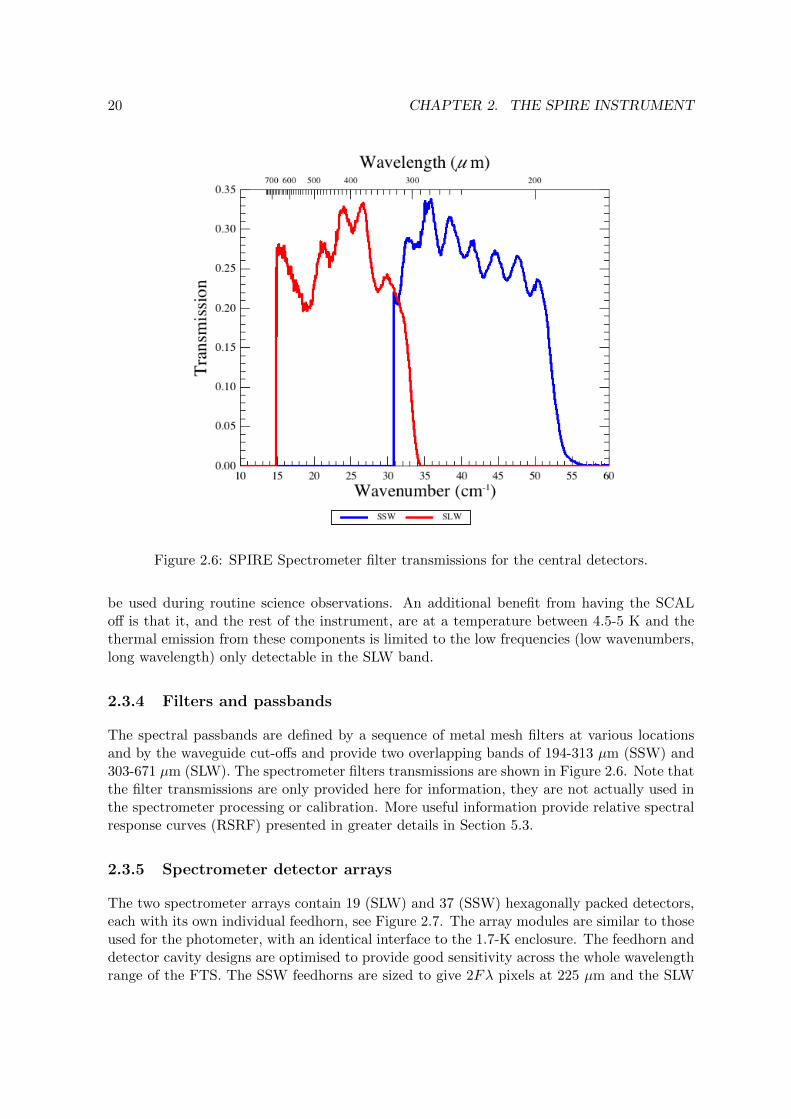
Figure 2.6: SPIRE Spectrometer filter transmissions for the central detectors.
be used during routine science observations. An additional benefit from having the SCALoff is that it, and the rest of the instrument, are at a temperature between 4.5-5 K and thethermal emission from these components is limited to the low frequencies (low wavenumbers,long wavelength) only detectable in the SLW band.
2.3.4 Filters and passbands
The spectral passbands are defined by a sequence of metal mesh filters at various locationsand by the waveguide cut-offs and provide two overlapping bands of 194-313 µm (SSW) and303-671 µm (SLW). The spectrometer filters transmissions are shown in Figure 2.6. Note thatthe filter transmissions are only provided here for information, they are not actually used inthe spectrometer processing or calibration. More useful information provide relative spectralresponse curves (RSRF) presented in greater details in Section 5.3.
2.3.5 Spectrometer detector arrays
The two spectrometer arrays contain 19 (SLW) and 37 (SSW) hexagonally packed detectors,each with its own individual feedhorn, see Figure 2.7. The array modules are similar to thoseused for the photometer, with an identical interface to the 1.7-K enclosure. The feedhorn anddetector cavity designs are optimised to provide good sensitivity across the whole wavelengthrange of the FTS. The SSW feedhorns are sized to give 2Fλ pixels at 225 µm and the SLW

2.4. COMMON INSTRUMENT PARTS 21
horns are 2Fλ at 389 µm. This arrangement has the advantage that there are many co-alignedpixels in the combined field of view. The SSW beams on the sky are 33 arcsec apart, and theSLW beams are separated by 51 arcsec. Figure 2.7 shows also the overlap of the two arrays onthe sky with circles representing the FWHM of the response of each pixel. The unvignettedfootprint on the arrays (diameter 2 arcmin) contains 7 pixels for SLW and 19 pixels for SSW,outside this circle the data is not-well calibrated. The design features of the detectors andfeedhorns are described in more detail in Section 2.4.1.
Figure 2.7: A schematic view of the FTS bolometer arrays, the bolometer names are alsoshown. Each circle represents a detector feedhorn. Those detectors centred on same sky posi-tions are shaded in blue, the dead bolometers are shaded in grey. The 2.6 arcmin unvignettedfield of view of each array is delineated by a red dashed circle. The two arrays overlap on thesky as shown in the rightmost figure, where the SLW and SSW are depicted by red and bluecircles respectively. The bold red circle delineates the 2 arcmin unvignetted field of view forFTS observations. The circle sizes in the rightmost figure correspond to the FWHM of thebeam. The spacecraft coordinate system (Y,Z) is also shown.
2.4 Common Instrument Parts
2.4.1 Basic bolometer operations
The SPIRE detectors for both the photometer and the spectrometer are semiconductorbolometers. The general theory of bolometer operation is described in Mather (1982) andSudiwala et al. (2002), and details of the SPIRE bolometers are given in Turner et al. (2001);Rownd et al. (2003) and Chattopadhaya et al. (2003).

22 CHAPTER 2. THE SPIRE INSTRUMENT
Figure 2.8: Basic principles of bolometer operation.
The basic features of a bolometer andthe principles of bolometer operation areoutlined here, and are illustrated in Fig-ure 2.8. The radiant power to be de-tected is incident on an absorber of heatcapacity C. Heat is allowed to flow fromthe absorber to a heat sink at a fixedtemperature T0 by a thermal conduc-tance, G (the higher G, the more rapidlythe heat leaks away). A thermometeris attached to the absorber, to sense itstemperature. A bias current, I, is passedthroughout the thermometer, and thecorresponding voltage, V , is measured.
The bias current dissipates electrical power, which heats the bolometer to a temperature, T ,slightly higher than T0. With a certain level of absorbed radiant power, Q, the absorber willbe at some temperature T , dictated by the sum of the radiant and electrical power dissipation.If Q changes, the absorber temperature will change accordingly, leading to a correspondingchange in resistance and hence in output voltage.
Figure 2.9: Magnified view of a SPIREbolometer, the thermometer size is10x100x300 µm.
In the case of the SPIRE detectors, the ab-sorber is a spider-web mesh composed of sil-icon nitride with a thin resistive metal coat-ing to absorb and thermalise the incident ra-diation. The thermometers are crystals ofNeutron Transmutation Doped (NTD) germa-nium, which has very high temperature coef-ficient of resistance. A magnified view of anactual SPIRE bolometer is shown in Figure2.9.
The main performance parameters for bolo-metric detectors are the responsivity (dV/dQ),the noise-equivalent power (NEP) and thetime constant (τ ∼ C/G). In order to achieve
high sensitivity (low NEP) and good speed of response, operation at low temperature isneeded. The photon noise level, arising from unavoidable statistical fluctuations in the amountof background radiation incident on the detector, dictates the required sensitivity. In the caseof SPIRE, this radiation is due to thermal emission from the telescope, and results in aphoton noise limited NEP on the order of a few ×10−17 W Hz−1/2. The bolometers are de-signed to have an overall NEP dominated by this contribution. To achieve this, the operatingtemperature for the SPIRE arrays must be of the order of 300 mK.
The operating resistance of the SPIRE bolometers is typically a few MΩ. The outputs are fedto JFETs located as close as possible to the detectors, in order to convert the high-impedancesignals to a much lower impedance output capable of being connected to the next stage ofamplification by a long cryoharness.
The thermometers are biased by an AC current, at a frequency in the 100-Hz region. This

2.4. COMMON INSTRUMENT PARTS 23
allows the signals to be read out at this frequency, which is higher than the 1/f knee frequencyof the JFETs, so that the 1/f noise performance of the system is limited by the detectorsthemselves, and corresponds to a knee frequency of around 100 mHz.
The detailed design of the bolometer arrays must be tailored to the background power thatthey will experience in flight, and to the required speed of response. The individual SPIREphotometer and spectrometer arrays have been optimised accordingly.
Figure 2.10: Photograph of a SPIRE detector arraymodule.
The bolometers are coupled to the tele-scope beam by conical feedhorns locateddirectly in front of the detectors on the3He stage. Short waveguide sections atthe feedhorn exit apertures lead into thedetector cavities. The feedhorn entranceaperture diameter is set at 2Fλ, where λis the design wavelength and F is the fi-nal optics focal ratio. This provides themaximum aperture efficiency and thusthe best possible point source sensitiv-ity (Griffin et al., 2002). The feedhornsare hexagonally close-packed, as shownin the photograph in Figure 2.10 andschematically in Figure 2.4 and Figure2.7, in order to achieve the highest pack-ing density possible. A centre-centre dis-tance of 2Fλ in the focal plane corre-sponds to a beam separation on the skyof 2λ/D, where D is the telescope di-ameter. This is approximately twice thebeam FWHM, so that the array does not
produce an instantaneously fully sampled image. A suitable scanning or multiple-pointing(“jiggling”) scheme is therefore needed for imaging observations.
2.4.2 3He cooler and thermal strap system
The same 3He cooler design (Duband et al., 1998), shown in Figure 2.11, is used for bothSPIRE and PACS instruments. This type of refrigerator consists of a sorption pump and anevaporator and uses porous material which absorbs or releases gas depending on its temper-ature. The refrigerator contains 6 litres of liquid 3He. At the beginning of the cold phase,all of this is contained in liquid form in the evaporator. The pump is cooled to ∼ 2 K, andcryo-pumps the 3He gas, lowering its vapour pressure and so reducing the liquid temperature.The slow evaporation of the 3He provides a very stable thermal environment at 300 mK foraround 48 hours under constant heat load in normal observing and operational circumstances.

24 CHAPTER 2. THE SPIRE INSTRUMENT
Figure 2.11: SPIRE cooler
Once most of the helium is evaporated and contained in thepump then the refrigerator must be recycled. This is carried outby heating of the sorption pump to ∼ 40 K in order to expel theabsorbed gas. The gas re-condenses as liquid at ∼ 2 K in theevaporator. Once all of the 3He has been recondensed, the pumpis cooled down again and starts to cryo-pump the liquid, bring-ing the temperature down to 0.3 K once again. This recyclingtakes about 2.5 hours and is usually performed during the dailytelecommunications period (DTCP). Gas gap heat switches con-trol the cooler and there are no moving parts. The confinementof the 3He in the evaporator at zero-g is achieved by a porousmaterial that holds the liquid by capillary attraction. A Kevlarwire suspension supports the cooler during launch whilst min-imising the parasitic heat load. Copper straps connect the cooler0.3 K stage to the five detector arrays, and are held rigidly at
various points by Kevlar support modules. The supports at the entries to the spectrometerand photometer 1.7 K boxes are also designed to be light-tight.
2.4.3 Warm electronics
There are three SPIRE warm electronics units. The Detector Control Unit (DCU) providesthe bias and signal conditioning for the arrays and cold electronics, and demodulates anddigitises the detector signals. The FPU Control Unit (FCU) controls the 3He cooler, the BeamSteering Mechanism and the FTS scan mirror, and also reads out all the FPU thermometers.The Digital Processing Unit (DPU) runs the on-board software interfaces with the spacecraftfor commanding and telemetry. The 130 kbs available data rate allows all photometer orspectrometer detectors to be sampled and the data transmitted to the ground with no on-board processing.

Chapter 3
Observing with SPIRE
3.1 Introduction
An observation with SPIRE (or any of the Herschel instruments) is performed following anAstronomical Observation Request (AOR) made by the observer. The AOR is constructedby the observer by filling in the so called Astronomical Observation Template (AOT) in theHerschel Observation Planning Tool, HSpot. Each template contains options to be selectedand parameters to be filled in, such as target name and coordinates, observing mode etc. Howto do this is explained in details in the HSpot user’s manual while in the relevant sections inthis chapter we explain the AOT user inputs.
Once the astronomer has made the selections and filled in the parameters on the template,the template becomes a request for a particular observation, i.e. an AOR. If the observationrequest is accepted via the normal proposal-evaluation-time allocation process then the AORcontent is subsequently translated into instrument and telescope/spacecraft commands, whichare up-linked to the observatory for the observation to be executed.
There are three Astronomical Observation Templates available for SPIRE: one for doingphotometry just using the SPIRE Photometer, one to do photometry in parallel with PACS(see The Parallel Mode Observers’ Manual for details on observing with this mode) and oneusing the Spectrometer to do imaging spectroscopy: this covers all spatial resolutions andhigh, medium or low spectral resolution.
Building Blocks: Observations are made up of logical operations, such as configuring theinstrument, initialisation and science data taking operations. These logical operations arereferred to as building blocks. The latter operations are usually repeated several times inorder to build up S/N and/or to map an area of sky. Pipeline data reduction modules workon building blocks (see Chapter 6).
Configuring and initialising the instrument: It is important to note that the configura-tion of the instrument, i.e. the bolometer parameters, like setting the bias, the science dataand housekeeping data rates etc., are only set once at the beginning of the observations withthis sub-instrument. There are however detector settings that are set up at the beginning ofeach observation, like the bolometer A/C offsets. It is not possible to change the settings dy-namically throughout an observation and this may have implications (mainly signal clipping
25

26 CHAPTER 3. OBSERVING WITH SPIRE
or signal saturation) for observations of very bright sources with strong surface brightnessgradients.
PCAL: During SPIRE observations, the photometer calibration source, PCAL, is operatedat intervals to track any responsivity drifts. Originally it was planned to use PCAL every45 minutes, but in-flight conditions have shown excellent stability and following performanceverification phase a new scheme has been adopted where PCAL is only used once at the endof an observation. This adds approximately 20 seconds to each photometer observation. Forthe spectrometer this can take a few seconds longer as the SMEC must be reset to its homeposition.
3.2 SPIRE Photometer AOT
This SPIRE observing template uses the SPIRE photometer (Section 2.2) to make simulta-neous photometric observations in the three photometer bands (250, 350 and 500 µm). It canbe used with three different observing modes:
• Large areas maps: This mode is for covering large areas of sky or extended sourceslarger than 5 arcmin diameter. The map is made by scanning the telescope.
• Small area maps: This is for sources or areas with diameters smaller than 5 arcmin.The map is made by two short cross-scans with the telescope.
• Point source photometry: This mode is for photometric observations of isolated pointsources. It uses chopping, jiggling and nodding, observing the source at all times.
3.2.1 Large Map
Description
The build up of a map is achieved by scanning the telescope at a given scan speed (Nominalat 30′′/s or Fast at 60′′/s) along lines. This is shown in Figure 3.1.
As the SPIRE arrays are not fully filled, the telescope scans are carried out at an angle of±42.4 deg with respect to the Z-axis of the arrays and the scan lines are separated by 348arcsec to provide overlap and good coverage for fully sampled maps in the three bands. Thisis shown schematically in Figure 3.1. One scan line corresponds to one building block.
Cross-linked scanning (or cross scanning) is achieved by scanning at +42.4 deg (Scan A angle)and then at −42.4 deg (Scan B angle), see Figure 3.3. The cross-scan at Scan A and B isthe default Large Map scan angle option in HSpot. This ensures improved coverage of themapped region. Although the 1/f knee for SPIRE is below 0.1 Hz (Griffin et al., 2010),the cross-scanning also help to reduce the effect of the 1/f noise when making maps withmaximum likelihood map makers like MADMAP(Cantalupo et al., 2010). Note that the 1/fnoise will be less significant at the faster scan speed.
Real coverage maps for the cross scanning and single direction scanning for the differentSPIRE bands can be found in Section 3.2.1.

3.2. SPIRE PHOTOMETER AOT 27
Figure 3.1: Large Map build up with telescope scanning, showing the scan angle, the scanlegs and the guaranteed map area.
When 1/f noise is not a concern, the observer can choose either one of the two possible scanangles, A or B. The two are equivalent in terms of observation time estimation, overheads,sensitivities, but one may be favourable, especially when the orientation of the arrays of thesky does not vary much (due to either being near the ecliptic or to having a constrainedobservation, see below).
To build up integration time, the map is repeated an appropriate number of times. For asingle scan angle, the area is covered only once. For cross-linked scanning, one repetitioncovers the area twice, once in each direction. Hence cross-linked scanning takes about twiceas long and gives better sensitivity (see e.g. Figure 3.6).
Cross-linked scanning is limited to an area of just under 4 degrees square, whereas singledirection scans can be up to nearly 20 degrees in the scan direction and just under 4 degreesin the other direction. Hence with a single scan direction it is possible to make very longrectangular maps. Note that cross-scan observations for highly rectangular areas are lessefficient as many shorter scans are needed in one of the directions.
The dimensions of the area to be covered are used to automatically set the length and thenumber of the scan legs. The scan length is set such that the area requested has good coveragethroughout the map and that the whole array passes over all of the requested area with thecorrect speed. The number of scan legs is calculated to ensure that the total area requestedby the user is observed without edge effects (a slightly larger area will be covered due to thediscrete nature of the scans). Hence the actual area observed will always be bigger than whatwas requested.

28 CHAPTER 3. OBSERVING WITH SPIRE
Figure 3.2: Large Map coverage showing the scan direction with respect to the SPIRE arrays,the scan leg separation step and the uniform sensitivity coverage region. The darker theshading the deeper the coverage.
The area is by default centred on the target coordinates; however this can be modified usingmap centre offsets (given in array coordinates). This can be useful when one wants to dodithering or to observe the core of an object plus part of its surroundings, but does not mindin which direction from the core the surrounding area is observed.
The scans are carried out at a specific angle to the arrays, and the orientation of the arrayson the sky changes as Herschel moves in its orbit. The actual coverage of the map will rotateabout the target coordinates depending on the exact epoch at which the data are taken(except for sources near the ecliptic plane where the orientation of the array on the sky isfixed: see the Herschel Observers’ Manual). This is shown in Figure 3.1.
To guarantee that the piece of sky you want to observe is included in the map, you canoversize the area to ensure that the area of interest is included no matter what the date ofobservation. This works well for square-like fields, but for highly elongated fields the oversizingfactor would be large. To reduce the amount of oversizing needed for the map you can use theMap Orientation “Array with Sky Constraint” setting to enter a pair of angles A1 and A2,which should be given in degrees East of North. The orientation of the map on the sky, withrespect to the middle scan leg, will be restricted within the angles given. This reduces theoversizing, but the number of days on which the observation can be scheduled is also reduced.
Note also that, as explained in Herschel Observers’ Manual, parts of the sky do not changetheir orientation with respect to the array and therefore it is not possible to set the orientationof the map in certain directions (the ecliptic) as the array has always the same orienatation.The constraints on when the observation can be performed make scheduling and the use ofHerschel less efficient, hence the observer will be charged 10 minutes observatory overheads(instead of 3 minutes) to compensate (see the Herschel Observers’ Manual).
Warning: Setting a Map Orientation constraint means that your observation can only beperformed during certain periods, and the number of days that your observation can be

3.2. SPIRE PHOTOMETER AOT 29
Figure 3.3: Large Map scan angles.
scheduled will be reduced from the number of days that the target is actually visible, becauseit is a constraint on the observation, not the target itself. In setting a constraint you willneed to check that it is still possible to make your observation.
User inputs
The user inputs in HSpot are shown Figure 3.4 and summarised below:
Repetition factor:The number of times the full map area is repeated to achieve the required sensitivity. Forcross-linked maps (Scan Angles A and B), there are two coverages per repetition, one ineach direction. For single scan direction observations (Scan Angle A or Scan Angle B), onecoverage is performed per repetition.
Length:This is the scan length of the map (in arcmin). It corresponds to the length in the first scandirection.
Height:This is the size of the map (in arcmin) in the other dimension.
The maximum allowed Length and Height for cross-linked large maps (Scan Angles A and B)are 226 arcmin for both directions. For scans in either Scan Angle A or Scan Angle B, themaximum Length is 1186 arcmin and the maximum Height is 240 arcmin.
Scan speed:This can be set as Nominal, 30′′/s (the default value) or Fast, 60′′/s.
Scan direction:The choices are Scan Angles A and B (the default option, giving a cross-linked map), ScanAngle A, or Scan Angle B.

30 CHAPTER 3. OBSERVING WITH SPIRE
Map centre offset Y, Z:This is the offset (in arcmin) of the map centre from the input target coordinates along theY or Z axes of the arrays. The minimum offset is ±0.1 arcmin and the maximum allowed is±300 arcmin.
Figure 3.4: Large Map parameters inHSpot
Map Orientation:This can be set at either Array or Array with SkyConstraint. The latter option can be entered by se-lecting a range of map orientation angles for the ob-servation to take place. The orientation angle is mea-sured from the equatorial coordinate system North tothe direction of the middle scan leg direction, positiveEast of North, following the Position Angle conven-tion. The orientation constraint means a schedulingconstraint and should therefore be used only if neces-sary.
Angle from/to:In the case when Array with Sky Constraint is se-lected, the pair of angles (in degrees) between whichthe middle scan leg can lie along.
Source Flux Estimates (optional):An estimated source flux density (in mJy) and/oran estimated extended source surface brightness(MJy/sr) may be entered for any of the three pho-tometer bands, in which case the expected S/N forthat band will be reported back in the Time Esti-mation. The sensitivity results assume that a pointsource has zero background and that an extendedsource is not associated with any point sources. Thepoint source flux density and the extended source sur-face brightness are treated independently by the sen-
sitivity calculations. If no value is given for a band, the corresponding S/N is not reportedback. The time estimation will return the corresponding S/N, as well as the original valuesentered, if applicable.Bright Source Setting (optional): this mode has to be selected if the expected flux of thesource is above 200 Jy (see Section 4.1.2).
Coverage Maps
Coverage maps for cross scanning and for single direction scanning for each of the threebands are shown in Figure 3.5. These were taken from standard pipeline processing of realobservations with SPIRE. Note that the coverage maps are given as number of bolometer hitsper sky pixel. The standard sky pixels for the SPIRE Photometer maps are (6, 10, 14) arcsec(see Section 4.1.1).

3.2. SPIRE PHOTOMETER AOT 31
Figure 3.5: Example coverage maps for Large Map mode for the three photometer arrays,PSW (left), PMW (centre) and PLW (right). The top row is for a single scan A observation.The bottom row is for a cross-linked scan of 30× 30 arcmin field, the white circle is the userrequested area. The pixel size is (6,10,14) arcsec for (PSW, PMW, PLW) and the colour coderepresents the number of bolometer hits in each sky pixel.
Time estimation and sensitivity
The estimated time to perform a single scan and cross-linked scans for one square degree field(60× 60 arcmin) and one repetitions are given in the HSpot screenshots in Figure 3.6.
The sensitivity estimates are subject to caveats concerning the flux density calibration (seeSection 5.2). The reported 1-σ noise level does not include the confusion noise, which ulti-mately limits the sensitivity (see Herschel Confusion Noise Estimator for more details). It isimportant to keep in mind that the galactic confusion noise can vary considerably over thesky.
When to use this mode
Large map mode is used to cover large fields, larger than 5 arcmin diameter, in the threeSPIRE photometer bands. Note that the mode can still be used even for input height and

32 CHAPTER 3. OBSERVING WITH SPIRE
Figure 3.6: Large Map time estimation and sensitivity for a filed of 60×60 and one repetitionfor a cross-linked (scan A and B, left) and single scan direction (right).
width of 5 arcmin, however the efficiency is low and the map size will be much larger thanthe requested 5x5 arcmin field.
The coverage map for a single scan observation is inhomogeneous due to missing or noisybolometers (see Figure 3.5). Even though the 1/f noise is not a big effect even for single scanmaps our advice is to use cross-linked maps when a better flux reconstruction is needed (i.e.deep fields, faint targets, etc).
3.2.2 Small Map
Description
The SPIRE Small Map mode is designed for observers who want a fully sampled map for asmall < 4 arcmin area of sky. The original SPIRE Small Map mode was initially a 64-pointJiggle Map. However, after analysis and investigation this has been replaced by a 1× 1 smallscan map using nearly orthogonal (at 84.8 deg) scan paths.
The Small Scan Map mode is defined as follows;
• 1x1 nearly orthogonal scan paths.
• Scan Angles are fixed at ±42.4 degrees with respect to the Spacecraft Z-axis.
• Fixed scan path with guaranteed coverage of 5 arcmin diameter circle.

3.2. SPIRE PHOTOMETER AOT 33
• Fixed scan speed = 30′′/s.
• Calibration PCAL flash made only at end of Observation.
• Map offsets available.
• Otherwise identical to the SPIRE Large Scan Map mode.
User inputs
The user inputs in HSpot are shown in Figure 3.7, left and described below.
Figure 3.7: User inputs in HSpot for Small Map AOT (left) and Small Map mode timeestimation, sensitivity estimate for one repetition of the map.
Repetition factor:The number of repeats of the 1x1 scan pattern.
Map Centre Offset Y and Z:This is the offset (in arcmin) of the map centre from the input target coordinates along theY or Z axis of the arrays. The minimum offset is ±0.1 arcmin and the maximum allowed is±300 arcmin.
Source Flux Estimates (optional):An estimated source flux density (in mJy) may be entered for a band, in which case theexpected S/N for that band will be reported back in the Time Estimation. The sensitivity
34 CHAPTER 3. OBSERVING WITH SPIRE
results assume that a point source has zero background. If no value is given for a band, thecorresponding S/N is not reported back.
Bright Source Setting (optional):this mode has to be selected if the expected flux of the source is above 200 Jy (see Section4.1.2).
Time estimation and sensitivity
The time estimation and sensitivities are shown in Figure 3.7, right. The sensitivity estimatesand the caveats are the same as the Large Map mode.
Coverage maps
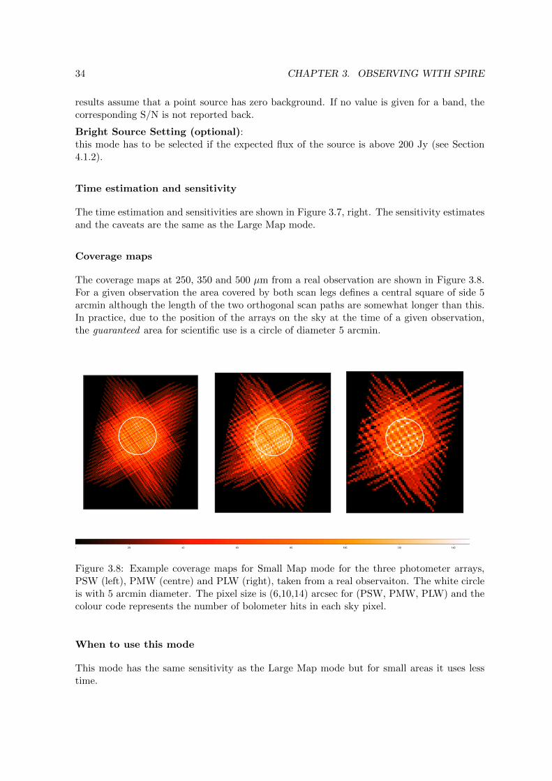
The coverage maps at 250, 350 and 500 µm from a real observation are shown in Figure 3.8.For a given observation the area covered by both scan legs defines a central square of side 5arcmin although the length of the two orthogonal scan paths are somewhat longer than this.In practice, due to the position of the arrays on the sky at the time of a given observation,the guaranteed area for scientific use is a circle of diameter 5 arcmin.
Figure 3.8: Example coverage maps for Small Map mode for the three photometer arrays,PSW (left), PMW (centre) and PLW (right), taken from a real observaiton. The white circleis with 5 arcmin diameter. The pixel size is (6,10,14) arcsec for (PSW, PMW, PLW) and thecolour code represents the number of bolometer hits in each sky pixel.
When to use this mode
This mode has the same sensitivity as the Large Map mode but for small areas it uses lesstime.
3.2. SPIRE PHOTOMETER AOT 35
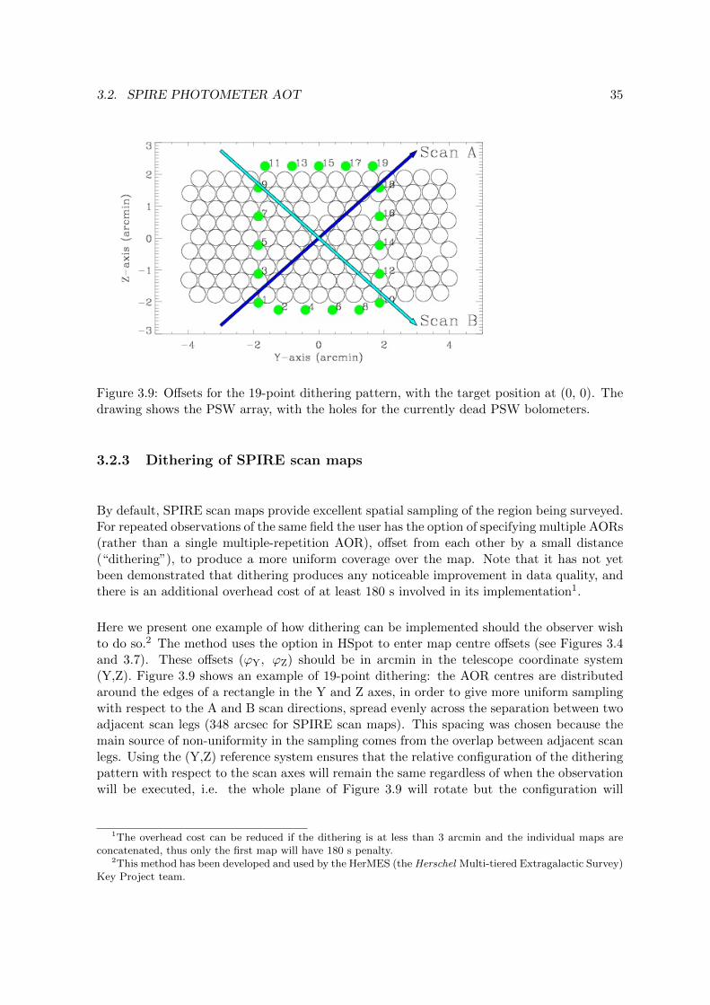
Figure 3.9: Offsets for the 19-point dithering pattern, with the target position at (0, 0). Thedrawing shows the PSW array, with the holes for the currently dead PSW bolometers.
3.2.3 Dithering of SPIRE scan maps
By default, SPIRE scan maps provide excellent spatial sampling of the region being surveyed.For repeated observations of the same field the user has the option of specifying multiple AORs(rather than a single multiple-repetition AOR), offset from each other by a small distance(“dithering”), to produce a more uniform coverage over the map. Note that it has not yetbeen demonstrated that dithering produces any noticeable improvement in data quality, andthere is an additional overhead cost of at least 180 s involved in its implementation1.
Here we present one example of how dithering can be implemented should the observer wishto do so.2 The method uses the option in HSpot to enter map centre offsets (see Figures 3.4and 3.7). These offsets (ϕY, ϕZ) should be in arcmin in the telescope coordinate system(Y,Z). Figure 3.9 shows an example of 19-point dithering: the AOR centres are distributedaround the edges of a rectangle in the Y and Z axes, in order to give more uniform samplingwith respect to the A and B scan directions, spread evenly across the separation between twoadjacent scan legs (348 arcsec for SPIRE scan maps). This spacing was chosen because themain source of non-uniformity in the sampling comes from the overlap between adjacent scanlegs. Using the (Y,Z) reference system ensures that the relative configuration of the ditheringpattern with respect to the scan axes will remain the same regardless of when the observationwill be executed, i.e. the whole plane of Figure 3.9 will rotate but the configuration will
1The overhead cost can be reduced if the dithering is at less than 3 arcmin and the individual maps areconcatenated, thus only the first map will have 180 s penalty.
2This method has been developed and used by the HerMES (the Herschel Multi-tiered Extragalactic Survey)Key Project team.
36 CHAPTER 3. OBSERVING WITH SPIRE
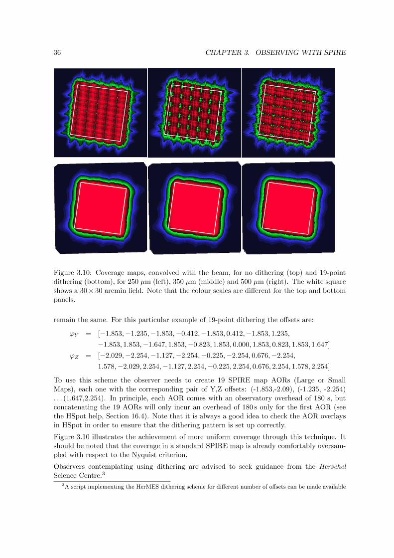
Figure 3.10: Coverage maps, convolved with the beam, for no dithering (top) and 19-pointdithering (bottom), for 250 µm (left), 350 µm (middle) and 500 µm (right). The white squareshows a 30× 30 arcmin field. Note that the colour scales are different for the top and bottompanels.
remain the same. For this particular example of 19-point dithering the offsets are:
ϕY = [−1.853,−1.235,−1.853,−0.412,−1.853, 0.412,−1.853, 1.235,
−1.853, 1.853,−1.647, 1.853,−0.823, 1.853, 0.000, 1.853, 0.823, 1.853, 1.647]
ϕZ = [−2.029,−2.254,−1.127,−2.254,−0.225,−2.254, 0.676,−2.254,
1.578,−2.029, 2.254,−1.127, 2.254,−0.225, 2.254, 0.676, 2.254, 1.578, 2.254]
To use this scheme the observer needs to create 19 SPIRE map AORs (Large or SmallMaps), each one with the corresponding pair of Y,Z offsets: (-1.853,-2.09), (-1.235, -2.254). . . (1.647,2.254). In principle, each AOR comes with an observatory overhead of 180 s, butconcatenating the 19 AORs will only incur an overhead of 180 s only for the first AOR (seethe HSpot help, Section 16.4). Note that it is always a good idea to check the AOR overlaysin HSpot in order to ensure that the dithering pattern is set up correctly.
Figure 3.10 illustrates the achievement of more uniform coverage through this technique. Itshould be noted that the coverage in a standard SPIRE map is already comfortably oversam-pled with respect to the Nyquist criterion.
Observers contemplating using dithering are advised to seek guidance from the HerschelScience Centre.3
3A script implementing the HerMES dithering scheme for different number of offsets can be made available

3.2. SPIRE PHOTOMETER AOT 37
Figure 3.11: Left: the 7-point hexagonal jiggle pattern. Note that the central point is revisitedat the end. The seven points are used to fit the 2-D beam as shown in the drawing. Right:the image shows the central co-aligned pixels as they appear on the sky. The circles numbered1 and 2 show the detectors on which a point source is viewed via the chopping and noddingwhich is described in detail in the text. The angular positions of detectors are also shown.
3.2.4 Point Source
Description
A mini-map is made around the nominal position to make sure that the source signal andposition can be estimated. This mini-map is made by moving the BSM around to make themap as shown in Figure 3.11 for one detector. The 7-point map is made by observing thecentral position and then moving the BSM to observe six symmetrically arranged positions(jiggle), offset from the central position by a fixed angle (nominally 6 arcsec), and thenreturning to the central point once more (note that the 7 in 7-point refers to the numberof different positions). At each of these positions chopping is performed between sets of co-aligned detectors (Figure 3.11, right) to provide spatial modulation and coverage in all threewavelength bands.
The chop direction is fixed along the long axis of the array (Y), and the chop throw is 126arcsec. The nominal chop frequency is 1 Hz. Sixteen chop cycles are performed at each jiggleposition. Nodding, once every 64 seconds, is performed along the Y axis to remove differencesin the background seen by the two detectors.
Figure 3.11, right, shows the central row of co-aligned pixels. At the first nod position (nod Aat 0,0) the source is repositioned with the BSM on detector 1 and the chopping is performedbetween 1 and 2. Then the telescope nods at +126 arcsec (as shown in the figure), this is nodB, and the target is repositioned with the BSM on detector 2. The chopping is between 2 and
upon request to the HSC helpdesk.
38 CHAPTER 3. OBSERVING WITH SPIRE
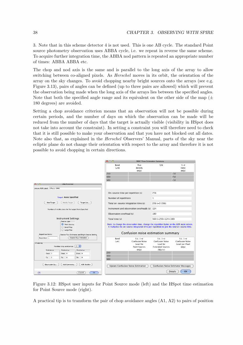
3. Note that in this scheme detector 4 is not used. This is one AB cycle. The standard Pointsource photometry observation uses ABBA cycle, i.e. we repeat in reverse the same scheme.To acquire further integration time, the ABBA nod pattern is repeated an appropriate numberof times: ABBA ABBA etc.
The chop and nod axis is the same and is parallel to the long axis of the array to allowswitching between co-aligned pixels. As Herschel moves in its orbit, the orientation of thearray on the sky changes. To avoid chopping nearby bright sources onto the arrays (see e.g.Figure 3.13), pairs of angles can be defined (up to three pairs are allowed) which will preventthe observation being made when the long axis of the arrays lies between the specified angles.Note that both the specified angle range and its equivalent on the other side of the map (±180 degrees) are avoided.
Setting a chop avoidance criterion means that an observation will not be possible duringcertain periods, and the number of days on which the observation can be made will bereduced from the number of days that the target is actually visible (visibility in HSpot doesnot take into account the constraint). In setting a constraint you will therefore need to checkthat it is still possible to make your observation and that you have not blocked out all dates.Note also that, as explained in the Herschel Observers’ Manual, parts of the sky near theecliptic plane do not change their orientation with respect to the array and therefore it is notpossible to avoid chopping in certain directions.
Figure 3.12: HSpot user inputs for Point Source mode (left) and the HSpot time estimationfor Point Source mode (right).
A practical tip is to transform the pair of chop avoidance angles (A1, A2) to pairs of position

3.2. SPIRE PHOTOMETER AOT 39
angles of the Herschel focal plane. Then, with the help of the HSpot target visibility tool,the days when the focal plane position angle does not fall between the derived angles can beidentified. As the chopping is on the Y-axis then the pair of chop avoidance angles (A1,A2)corresponds to two pairs of Herschel focal plane position angles (PA1,PA2) = (A1, A2) ± 90,which have to be avoided.
Warning: The constraints on when the observation can be performed make scheduling andthe use of Herschel less efficient. The observer will be charged extra 10 minutes in overheads(rather than the usual 3) to compensate.
Table 3.1: The basic parameters for the Point Source mode.
Parameter Value
Chop Throw 126 arcsec (± 63 arcsec)Chopping frequency 1HzJiggle position separation 6 arcsecNod Throw 126 arcsec (± 63 arcsec)Central co-aligned detector PSW E6, PMW D8, PLW C4Off-source co-aligned detectors PSW E2,E10, PMW D5,D11, PLW C2,C6Number of ABBA repeats 1Integration time 256 sInstrument/observing overheads 124 sObservatory overheads 180 sTotal Observation Time 560 s
User Inputs
The user input in HSpot are shown in Figure 3.12 and explained below.
Repetition factor:The number of times the nod cycle ABBA is repeated to achieve the required sensitivity.
Number of chop avoidances:An integer between 0 and 3.
Chopping Avoidance Angles From/To:To be used when number of chop avoidances is greater than zero. A From/To pair defines arange of angles to be avoided. Note that also the range ±180 degrees is also avoided. Theinterval is defined in equatorial coordinates, from the celestial north to the +Y spacecraft axis(long axis of the bolometer), positive East of North, following the Position Angle convention.This effectively defines an avoidance angle for the satellite orientation, and hence it is ascheduling constraint.
Source Flux Estimates (optional):An estimated source flux density (in mJy) may be entered for a band, in which case theexpected S/N for that band will be reported back in the Time Estimation. The sensitivityresults assume that a point source has zero background. If no value is given for a band, thecorresponding S/N is not reported back.Bright Source Setting (optional): this mode has to be selected if the expected flux of thesource is above 200 Jy (see Section 4.1.2).

40 CHAPTER 3. OBSERVING WITH SPIRE
Time estimation and sensitivity
The SPIRE Point Source mode is optimised for observations of relatively bright isolated pointsources. In this respect the accuracy of the measured flux is more relevant than the absolutesensitivity of the mode. The noise will be a function of three contributions. For a singleABBA repetition;
• The instrumental noise will be a constant value.
• There will be some underlying confusion noise which will vary from field to field.
• There will be a flux dependent uncertainty introduced by pointing jitter that will besome fraction of the total flux.
The current 1 σ instrumental noise uncertainties for a single ABBA repetition using thecentral co-aligned detector are tabulated in Table 3.2 and the HSpot screenshot is shown inFigure 3.12. The instrumental noise decreases as the reciprocal of the square root of thenumber of ABBA repetitions however note that the instrumental noise for a single repetitionof this mode is expected to equal the extragalactic confusion noise, for sources fainter than 1Jy.
Table 3.2: Point source mode sensitivities.
Source flux range 1 σ instrumental noise level250 µm 350 µm 500 µm
0.2-1 Jy 7 mJy 7 mJy 7 mJy< 4 Jy S/N ∼ 200> 4 Jy S/N ∼ 100
When to use this mode
The SPIRE Point Source mode is recommended for bright isolated sources in the range 0.2-4Jy where the astrometry is accurately known and accurate flux measurement is required. Forsources fainter than 200mJy (where the background produces a significant contribution) orat fluxes higher than ∼ 4 Jy (where pointing jitter can introduce large errors) the Small Mapmode is preferable.
For Point Source mode, the effective sky confusion level is increased due to chopping andnodding (by a factor of approximately 22% for the case of extragalactic confusion noise) andshould be added in quadrature to the quoted instrumental noise levels. The result of themeasurement is therefore affected by the specific characteristics of the sky background inthe vicinity of the source and will depend on the chop/nod position angle in the event ofan asymmetric background. Note that although it is possible to set a chop avoidance anglewithin HSpot this will constrain the possible dates for the observation
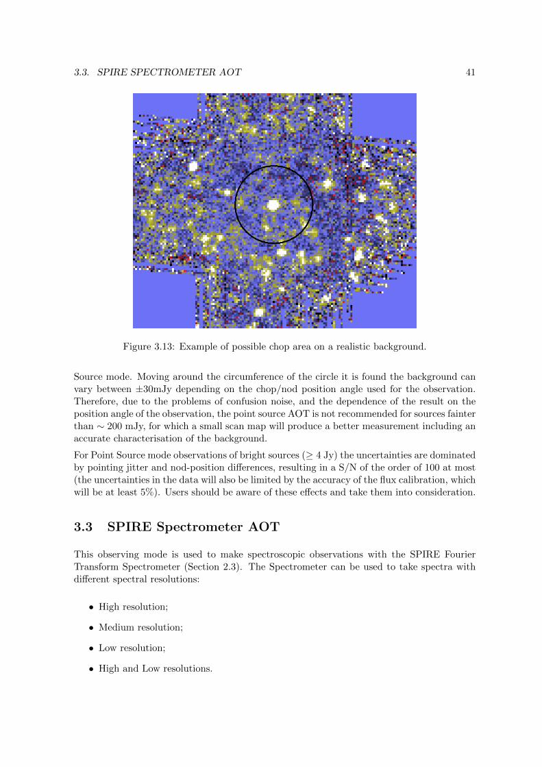
The example in Figure 3.13 shows a scan map observation of a ∼ 220 mJy source. Thecircle drawn around the source corresponds to the chop and/or nod throw used in the Point
3.3. SPIRE SPECTROMETER AOT 41
Figure 3.13: Example of possible chop area on a realistic background.
Source mode. Moving around the circumference of the circle it is found the background canvary between ±30mJy depending on the chop/nod position angle used for the observation.Therefore, due to the problems of confusion noise, and the dependence of the result on theposition angle of the observation, the point source AOT is not recommended for sources fainterthan ∼ 200 mJy, for which a small scan map will produce a better measurement including anaccurate characterisation of the background.
For Point Source mode observations of bright sources (≥ 4 Jy) the uncertainties are dominatedby pointing jitter and nod-position differences, resulting in a S/N of the order of 100 at most(the uncertainties in the data will also be limited by the accuracy of the flux calibration, whichwill be at least 5%). Users should be aware of these effects and take them into consideration.
3.3 SPIRE Spectrometer AOT
This observing mode is used to make spectroscopic observations with the SPIRE FourierTransform Spectrometer (Section 2.3). The Spectrometer can be used to take spectra withdifferent spectral resolutions:
• High resolution;
• Medium resolution;
• Low resolution;
• High and Low resolutions.

42 CHAPTER 3. OBSERVING WITH SPIRE
Spectra can be measured in a single pointing (using a set of detectors to sample the fieldof view of the instrument) or in larger maps which are made by moving the telescope in araster. For either of these, it is possible to choose sparse, intermediate, or full Nyquist spatialsampling. In summary, to define an observation, one needs to select a spectral resolution (high,medium, low, high and low), an image sampling (sparse, intermediate, full) and a pointingmode (single or raster). These options are described in more detail in the next sections. Forworked examples of how to combine these modes together to produce observations see Section3.4.
The HSpot input parameters for all SPIRE Spectrometer observing modes are shown in Figure3.14. In the following sections we describe each one of the options.
Figure 3.14: The HSpot initial screen for the SPIRE Spectrometer AOTs, point source mode(left) and raster (right)
3.3.1 Spectral Resolution
The Spectrometer Mirror Mechanism (SMEC) is scanned continuously at constant speed overdifferent distances to give different spectral resolutions (see Section 2.3). For every repetition,two scans of the SMEC are done: one in the forward direction and one in the backwarddirection, making one scan pair, as shown in Figure 3.15. Two scan pairs are deemed essentialfor redundancy in the data. The desired integration time is set by increasing the number ofscan pairs performed (corresponding to the number of repetitions entered in HSpot).

3.3. SPIRE SPECTROMETER AOT 43
Figure 3.15: Diagram to show how the SMEC moves (in terms of optical path difference)during one repetition for High, Medium and Low spectral resolution. The low resolutionSMEC scan range is always covered during High or Medium resolution observations.
Low Resolution:
Usage and Description: To make continuum measurements at the resolution of ∆σ = 0.83cm−1 (λ/∆λ = 48 at λ = 250µm, see Figure 4.3). The SMEC is scanned symmetricallyabout ZPD over a short distance. It takes 6.4 s to perform one scan in one direction atlow resolution. This mode is intended to survey sources without spectral lines or very faintsources where only an SED is required.
Medium Resolution:
Usage and Description: The intermediate resolution of ∆σ = 0.24 cm−1 (λ/∆λ = 160at λ = 250µm, see Figure 4.3) will be more suited to broad features. Medium resolutionscans are made by scanning the SMEC again symmetrically about ZPD, but over a largerdistance than in the low resolution mode. It takes 24.4 s to perform one scan in one directionat medium resolution. This mode is intended for surveys where the user may require asignificant amount of spatial coverage and also wishes to survey bright, isolated lines. Forthese cases the high resolution mode may take too much observing time. This mode mayalso be useful to characterise the SED with more data points than available with low spectralresolution.
High Resolution:
Usage and Description: The high resolution mode gives spectra at the highest resolutionavailable with the SPIRE spectrometer, ∆σ = 0.04 cm−1 (1.2 GHz) which corresponds toλ/∆λ = 1000 at λ = 250µm (see Figure 4.3). High resolution scans are made by scanningthe SMEC to the maximum possible distance from ZPD. It takes 66.6 s to perform one scanin one direction at high resolution. This mode is best for discovery spectral surveys wherethe whole range from 194 to 671 µm can be surveyed for new lines. It is also useful forsimultaneously observing sequences of spectral lines across the band (e.g. the CO rotationalladder). In this way, a relatively wide spectral range can be covered in a short amount of

44 CHAPTER 3. OBSERVING WITH SPIRE
time compared to using HIFI (although with much lower spectral resolution than achievedby HIFI, see the HIFI Observers’ Manual).
The Instrumental Line Shape of the SPIRE spectrometer is a Sinc function (see Figure 4.2)and the FWHM of an unresolved spectral line will be 1.207 times the spectral resolution, i.e.0.048 cm−1 for a high resolution spectrum. The FWHM in km/s for the high and the mediumresolution mode are shown in Figure 4.3.
Low resolution spectra are also extracted by the pipeline from high and medium resolutionobservations. Consequently, the equivalent low resolution continuum rms noise (for the num-ber of scan repetitions chosen) can also be recovered from a high resolution observation – i.e.improving the sensitivity to the continuum.
For cases where the S/N ratio for this extracted low resolution spectrum is not sufficient forthe scientific case, the following “High and Low” resolution mode is available:
High and Low Resolution:
Usage and Description: This mode allows to observe a high resolution spectrum as wellas using additional integration time to increase the S/N of the low resolution continuum toa higher value than would be available from using a high resolution observation on its own.This mode saves overhead time over doing two separate observations.
The number of high resolution and low resolution scans can differ, and will depend on therequired S/N for each resolution. If the number of repetitions for the high and low resolutionparts are nH and nL respectively, then the achieved low resolution continuum sensitivity willcorrespond to nH+nL repetitions, because low resolution data can also be extracted fromevery high resolution scan.
It is up to the observer to decide if this mode, or a single high resolution observation ismore suitable (in terms of sensitivities) for their scientific objectives. For examples of theseconsiderations see Section 3.4.
3.3.2 Pointing Modes
A pointing mode and an image sampling are combined to produce the required sky coverage.Here the pointing modes are described.
Single Pointing Mode:
Usage and Description: This is used to take spectra of a region covered by the instrumentfield of view (2 arcmin diameter circle unvignetted). With one pointing of the telescope onlythe field of view of the arrays on the sky is observed.
Raster Pointing Mode:
Usage and Description: This is used to take spectra of a region larger than the field ofview of the instrument (2 arcmin diameter circle unvignetted). The telescope is pointed tovarious positions making a hexagonally packed map (see example in Figure 3.16). At each
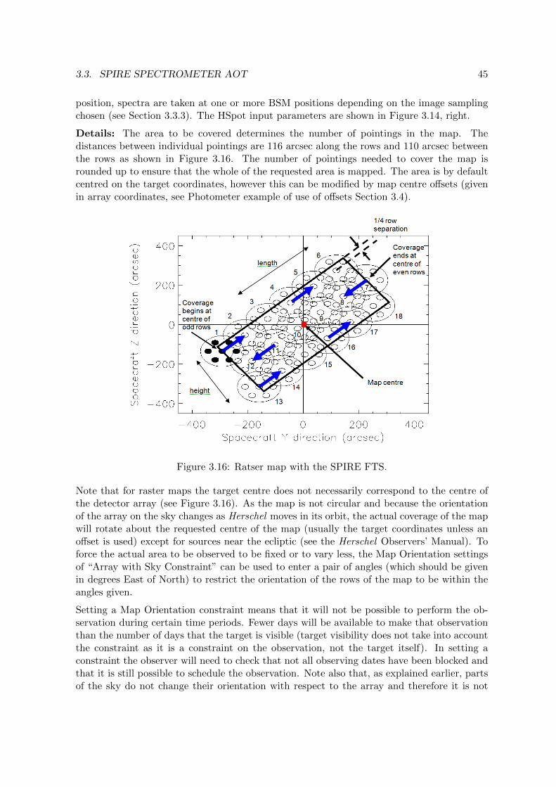
3.3. SPIRE SPECTROMETER AOT 45
position, spectra are taken at one or more BSM positions depending on the image samplingchosen (see Section 3.3.3). The HSpot input parameters are shown in Figure 3.14, right.
Details: The area to be covered determines the number of pointings in the map. Thedistances between individual pointings are 116 arcsec along the rows and 110 arcsec betweenthe rows as shown in Figure 3.16. The number of pointings needed to cover the map isrounded up to ensure that the whole of the requested area is mapped. The area is by defaultcentred on the target coordinates, however this can be modified by map centre offsets (givenin array coordinates, see Photometer example of use of offsets Section 3.4).
Figure 3.16: Ratser map with the SPIRE FTS.
Note that for raster maps the target centre does not necessarily correspond to the centre ofthe detector array (see Figure 3.16). As the map is not circular and because the orientationof the array on the sky changes as Herschel moves in its orbit, the actual coverage of the mapwill rotate about the requested centre of the map (usually the target coordinates unless anoffset is used) except for sources near the ecliptic (see the Herschel Observers’ Manual). Toforce the actual area to be observed to be fixed or to vary less, the Map Orientation settingsof “Array with Sky Constraint” can be used to enter a pair of angles (which should be givenin degrees East of North) to restrict the orientation of the rows of the map to be within theangles given.
Setting a Map Orientation constraint means that it will not be possible to perform the ob-servation during certain time periods. Fewer days will be available to make that observationthan the number of days that the target is visible (target visibility does not take into accountthe constraint as it is a constraint on the observation, not the target itself). In setting aconstraint the observer will need to check that not all observing dates have been blocked andthat it is still possible to schedule the observation. Note also that, as explained earlier, partsof the sky do not change their orientation with respect to the array and therefore it is not

46 CHAPTER 3. OBSERVING WITH SPIRE
possible to set the orientation of the map in certain directions (the ecliptic) as the array isonly orientated in one way on the sky. These constraints on when the observation can beperformed make scheduling and the use of Herschel less efficient, hence the observer will becharged extra overheads to compensate.
Alternatively, raster observations can be split into several concatenated AORs to allow sometailoring of the coverage to match the source shape - see Section 3.4 for an example (but notethat every concatenated AOR will be charged the 180 second slew tax).
User Input: The map parameters are similar to those for the Photometer Large Map. TheSpectrometer parameters are listed in Section 3.3.4.
Figure 3.17: Spectrometer raster example to show spacing of the individual pointings for thelong wavelength array (SLW, left) and the short wavelength array (SSW, right) for interme-diate image sampling.
3.3.3 Image Sampling
The pointing and an image sampling mode are combined to produce the required sky coverage.Here the image sampling options are described and figures are given to show the sampling.
Note that the figures show only the unvignetted detectors. Detailed calibration for data fromthe non-central detectors will be more demanding than for the central detectors.
Sparse Image Sampling:
Usage and Description: In conjunction with a single pointing, to measure the spectrumof a point or compact source well centred on the central detectors of the Spectrometer. Toprovide sparse maps (either for a single pointing or a raster grid of pointings). The BSMis not moved during the observation, producing a single array footprint on the sky. Theresult is an observation of the selected source position plus a hexagonal-pattern sparse mapof the surrounding region with beam centre spacing of (32.5, 50.5) arcsec in the (SSW, SLW)bands as shown in Figure 3.18. For a point source this requires accurate pointing and reliableknowledge of the source position to be sure to have the source well centred in the (central)detector beam.

3.3. SPIRE SPECTROMETER AOT 47
Figure 3.18: SPIRE Spectrometer spatial sampling: sparse (left), intermediate (centre) andfull (right). The small green and magenta circles indicate the regions where spectra will beobserved for different spatial samplings. The green circles show SSW and the magenta showSLW, the large red circle of 2 arcmin diameter is to guide the eye for the unvignetted field ofview.
Intermediate Image Sampling:
Usage and Description: This is to produce imaging spectroscopy with intermediate spatialsampling (1 beam spacing). This gives intermediate spatial sampling without taking as longas a fully Nyquist sampled map. This is achieved by moving the BSM in a 4-point lowfrequency jiggle, giving a beam spacing of (16.3, 25.3) arcsec in the final map as shown inFigure 3.18 and Figure 3.19. The input number of repetitions is performed at each of the 4positions to produce the spectra. The coverage maps for the SSW and SLW in this mode areshown in Figure 3.20, left column.
Full Image Sampling:
Usage and Description: This allows fully Nyquist sampled imaging spectroscopy of aregion of the sky or an extended source. This is achieved by moving the BSM in a 16-pointjiggle to provide complete Nyquist sampling (1/2 beam spacing) of the required area. Thebeam spacing in the final map is (8.1, 12.7) arcsec as shown in Figure 3.18 and in Figure 3.19.The input number of repetitions is performed at each one of the 16 positions to produce thespectra. The coverage maps for the SSW and SLW in this mode are shown in Figure 3.20,right column.
3.3.4 User input parameters for all Spectrometer AOTs.
The user inputs shown in Figure 3.14 are given below:
Pointing Mode:Single Pointing or Raster selection. See Section 3.3.2 for details. Note that if Raster is selectedthen size of the map (Length and Height) must be given.
Image Sampling:Sparse, Intermediate or Full. See Section 3.3.3 for details.

48 CHAPTER 3. OBSERVING WITH SPIRE
Figure 3.19: The FTS mapping pattern with intermediate image sampling for SSW and SLW(4-point jiggle, top) and full sampling (16 point jiggle, bottom). The red circle shows the 2arcmin unvignetted field of view of the FTS. The spacing of the beams is indicated for eachof the detector arrays and the two image sampling modes. The red dots show the centraldetector of each array at the 4 jiggle positions (top) and the 16 jiggle positions (bottom).
Spectral Resolution:High, Medium, Low or High and Low. See Section 3.3.1 for details.
Repetition factor:The number of spectral scan pairs to be made at each position. Note that if High and Lowresolution is selected you can independently control the number of pairs for each resolution.
Length:In arcmin. The length of the raster map along the rows.
Height:In arcmin. The height of the raster map.
Map centre offset Y, Z:In arcmin. The offset of the raster map centre from the input target coordinates along the Yor Z axes of the arrays. Minimum is ±0.1 arcmin, maximum ±300 arcmin.
Map Orientation:Either Array or Array with Sky Constraint. If Array with Sky Constraint is selected thenrange of the map orientation is constrained. This is a scheduling constraint and should

3.3. SPIRE SPECTROMETER AOT 49
Figure 3.20: Intermediate (top) and Full (bottom) spatial sampling coverage maps for SLW(left) and SSW (right) from a real SPIRE FTS mapping observation. The sky spectral pixel(spaxel) sizes are 35 arcsec (top left), 17.5 arcsec (bottom left), 19 arcsec (top right), 9.5arcsec (bottom right). The number of bolometer hits in each sky pixel are encoded withcolour. The holes in the maps, due to dead bolometers, depend on the spacecraft attitude(the focal plane position angle), the grid centre, the pixel scale.
therefore only be used if necessary.
Angle from/to:In degrees East of North. In the case that Array with Sky Constraint is selected, the anglesbetween which the raster rows can be constrained to are entered here.
Source Flux Estimates:Optional: if the estimated line flux in 10−17 W m−2, and/or the estimated continuum (se-lectable units either Jy or 10−17 W m−2 µm−1) is entered along with a wavelength then theexpected S/N for that line or continuum will be reported back in the Time Estimation aswell as the original values entered. The time estimator always returns 1-σ flux sensitivity,1-σ continuum sensitivity and unapodised resolving power for 8 standard wavelengths. Note,when Low resolution is selected only continuum information can be entered and returned(plus the unapodised resolving power). When High and Low resolution is selected data arereturned for the two different resolutions, the low resolution sensitivity does not take intoaccount the possibility to get the low resolution part from the high resolution spectrum.
Bright source mode:Optional: when the source is expected to be very bright (see Section 5.3.4 for more details)then this option provides a way to switch the detectors to bright mode settings, thus avoidingsignal clipping. Using this mode leads to 25 s increase in the overhead time, because thedetector A/C offsets are set at the start of the observation at each jiggle position.
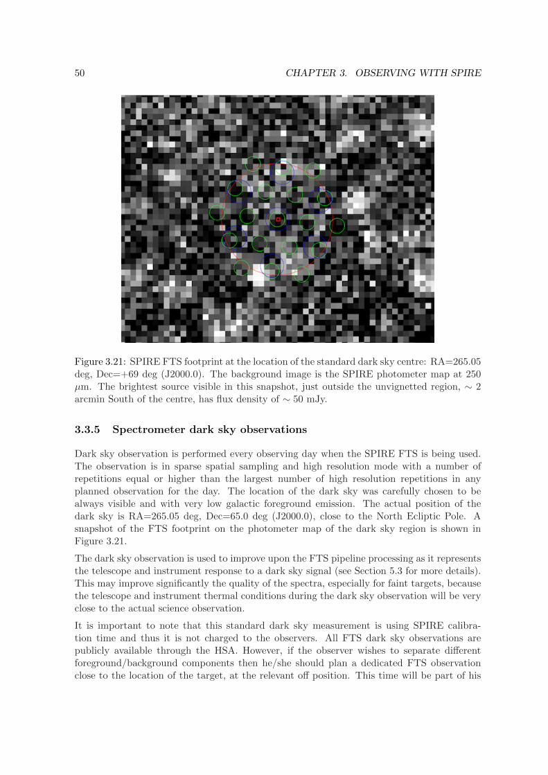
50 CHAPTER 3. OBSERVING WITH SPIRE
Figure 3.21: SPIRE FTS footprint at the location of the standard dark sky centre: RA=265.05deg, Dec=+69 deg (J2000.0). The background image is the SPIRE photometer map at 250µm. The brightest source visible in this snapshot, just outside the unvignetted region, ∼ 2arcmin South of the centre, has flux density of ∼ 50 mJy.
3.3.5 Spectrometer dark sky observations
Dark sky observation is performed every observing day when the SPIRE FTS is being used.The observation is in sparse spatial sampling and high resolution mode with a number ofrepetitions equal or higher than the largest number of high resolution repetitions in anyplanned observation for the day. The location of the dark sky was carefully chosen to bealways visible and with very low galactic foreground emission. The actual position of thedark sky is RA=265.05 deg, Dec=65.0 deg (J2000.0), close to the North Ecliptic Pole. Asnapshot of the FTS footprint on the photometer map of the dark sky region is shown inFigure 3.21.
The dark sky observation is used to improve upon the FTS pipeline processing as it representsthe telescope and instrument response to a dark sky signal (see Section 5.3 for more details).This may improve significantly the quality of the spectra, especially for faint targets, becausethe telescope and instrument thermal conditions during the dark sky observation will be veryclose to the actual science observation.
It is important to note that this standard dark sky measurement is using SPIRE calibra-tion time and thus it is not charged to the observers. All FTS dark sky observations arepublicly available through the HSA. However, if the observer wishes to separate differentforeground/background components then he/she should plan a dedicated FTS observationclose to the location of the target, at the relevant off position. This time will be part of his
3.4. USING HSPOT TO PREPARE AOR 51
observation and will be charged to his science programme.
3.3.6 Considerations when preparing FTS observations
There are some important considerations to be taken into account when preparing FTS ob-servations. These are based on our current knowledge of the FTS performance. Most of themare described in details in this chapter as well as in Chapters 4 and 5.
Spectral resolution: The use of medium spectral resolution (MR) is suggested only forbright, isolated lines or for broad-band features.
SED-like mode: The use of low or medium spectral resolution to get the overall spectralenergy distribution is not recommended without SPIRE photometry observation: theremoval of the telescope and instrument background may lead to significant offsets inthe absolute continuum level.
Long observations: The rms noise in HR observations with ∼ 100 repetitions (4 hours)beats down following the
√time law. Longer observations are better to be split into
AORs with no more than 100-120 repetitions as there is no guarantee that instrumentstability issues will not have considerable impact on the observation.
Mapping: For fully sampled maps, spatial pixels in the spectral cube can be co-added/resizedto enhance sensitivity. Calibration errors or other imperfections, however, may lead toworse signal-to-noise than achievable in theory.
Background: Dark sky observation is always performed during FTS observing days, this ispart of the SPIRE instrument calibration time. If a local background/foreground needsto be separated from the source then it is up to the observer to define the location andthe depth of this observation. It will be part of the proposal.
We strongly encourage the observers to contact the FTS User Support Group, via the Herschelhelpdesk, whenever they have questions or need assistance regarding the use the FTS.
3.4 Using HSpot to prepare AOR
This section lists screencast tutorials available as an on-line material from the HSC web pages.Note that the video tutorials are without an audio recording.
• Photometer observations
– Small Map AOR:In this tutorial: how to fill in a target, change AOR label, check visibility, checkthe time estimation and achieved sensitivity, input estimated flux for the source toget the S/N, overlay the AOR on an image.http://herschel.esac.esa.int/Docs/SPIRE/Videos/small-map-video.mov

52 CHAPTER 3. OBSERVING WITH SPIRE
– Large Map AOR:In this tutorial: how to fill in a target, change AOR label, check visibility, checkthe time estimation and achieved sensitivity, overlay the AOR on an image, setmap orientation constraints.http://herschel.esac.esa.int/Docs/SPIRE/Videos/large-map-video.mov
– Point Source AOR:In this tutorial: how to fill in a target, change AOR label, check visibility, checkthe time estimation and achieved sensitivity, input estimated flux for the sourceto get the S/N, overlay the AOR on an image, set up chop avoidance angles.http://herschel.esac.esa.int/Docs/SPIRE/Videos/point-source-video.
mov
• Spectrometer observations
– Point source, sparse map AOR:In this tutorial: how to fill in a target, change AOR label, check visibility andbackground, check the time estimation and achieved sensitivity, input estimatedflux for the source to get the S/N, overlay the AOR on an image.http://herschel.esac.esa.int/Docs/SPIRE/Videos/fts-sparse-video.mov

Chapter 4
SPIRE in-flight performance
The performance of SPIRE was estimated prior to launch using a detailed model of theinstrument and the telescope and the results of instrument-level and Herschel system-leveltests. Some details of the model assumptions and adopted parameters are given in e.g.,Griffin (2008). Based on the optimisation and evaluation of the instrument performanceduring Commissioning and Performance Verification phases, and further checks using ScienceDemonstration phase observations, the in-flight performance of the photometer and FTS havenow been assessed, and HSpot has been updated accordingly. In this section we summarisethe achieved in-flight performance.
4.1 Photometer performance
4.1.1 Beam profiles
The photometer beam profiles have been measured using scan maps of Neptune, which pro-vides high S/N and appears point-like in all bands. The beams are well described by 2-DGaussians down to ∼ 15 dB, with FWHM values and detailed side-lobe structure in goodagreement with the pre-launch optical model of the instrument and telescope system. Thebasic beam parameters vary as a function of the pixel scale used in the beam map, withthe FWHM values and beam areas increasing with pixel size as the fidelity of the surfacebrightness reconstruction becomes less reliable at low resolution, particularly with respectto the Airy ring pattern at higher radii from the source peak. The basic beam parameters,determined by fitting a 2-D asymmetric Gaussian to the data binned into pixels of 1 arcsecside and pixels of the standard sizes used for SPIRE Level-2 maps (6, 10, 14) arcsec per pixelat (250, 350, 500) µm are given in Table 4.1. These figures represent an average over eacharray; there are small systematic variations at the level of ∼ 5% across the arrays.
The beam maps and parameters, and their use in calibration of extended emission in SPIREmaps, are described in more detail in Chapter 5.
53

54 CHAPTER 4. SPIRE IN-FLIGHT PERFORMANCE
Table 4.1: Basic Gaussian parameters for measured beams with a 1 arcsec pixel size and forthe nominal SPIRE Level-2 map pixel sizes (6, 10, 14)”. Uncertainties in the beam FWHMvalues and areas are estimated at < 1%. See Section 5.2.7 for more details.
Pixelsize
Band MajoraxisFWHM
MinoraxisFWHM
GeometricmeanFWHM
Ellipticity
(µm) (arcsec) (%)
1 250 18.3 17.0 17.6 8.11 350 24.7 23.2 23.9 6.61 500 37.0 33.4 35.1 10.9
6 250 18.7 17.5 18.2 7.410 350 25.6 24.2 24.9 6.114 500 38.2 34.6 36.3 10.1
4.1.2 Sensitivity
The photometer sensitivity in scan map mode has been estimated from repeated scan mapsof dark regions of extragalactic sky. A single map repeat is constituted by two orthogonalscans as implemented in the SPIRE-only scan-map AOT. Multiple repeats produce a mapdominated by the fixed-pattern sky confusion noise, with the instrument noise having inte-grated down to a negligible value. This sky map can then be subtracted from individualrepeats to estimate the instrument noise. The extragalactic confusion noise levels for SPIREare assessed in detail by Nguyen et al. (2010), who define confusion noise as the standarddeviation of the flux density in the map in the limit of zero instrument noise. The measuredextragalactic confusion and instrument noise levels are given in Table 4.2 for the nominalscan speed (30′′/s). Instrument noise integrates down in proportion to the square root of thenumber of repetitions, and for the fast scan speed (60′′/s) the instrument noise is
√2 higher
as expected from the factor of 2 reduction in integration time per repeat. The achieved in-strument noise levels are comparable to the pre-launch estimates which were (9.6, 13.2, 11.2)mJy in beam at (250, 350, and 500) µm – very similar for the 250 and 500 µm bands andsomewhat better for the 350 µm band. In SPIRE-PACS Parallel mode, the achieved SPIREinstrument noise level per repeat is different to that for a single repeat in SPIRE-only modedue to the different effective integration time per beam (see the SPIRE-PACS Parallel ModeObservers’ Manual).
Figure 4.1 shows the manner in which the overall noise integrates down as a function ofrepeats for cross-linked maps with the nominal 30′′/s scan rate. The overall noise is within afactor of
√2 of the (250, 350, 500) µm confusion levels for (3, 2, 2) repeats.
Notes:
1. All sensitivity values correspond to nominal source strength settings. For bright sourcesettings, recommended for sources brighter than 200 Jy in any band, the achievedsensitivities are degraded (with respect to nominal setting) by factors of (3.8, 3.2, 2.6)

4.1. PHOTOMETER PERFORMANCE 55
Figure 4.1: Pixel noise vs. integration time for all pixels in deep SPIRE photometer fields.The derived instrument noise is shown in red, the confusion floor is show in blue and the totalnoise is in green. Taken from Nguyen et al. (2010).
for (250, 350, 500) µm. It should be noted however, that in practice S/N values > 200should not be regarded as reliable in any case.
2. All scan map sensitivity values are for nominal scan speed of 30”/s. Figures for 60”/sscale as
√2.
3. For Point Source mode (7-point jiggle) observations, the effective sky confusion levelis increased due to chopping and nodding. The result of the measurement is thereforeaffected by the detailed characteristics of the sky background in the vicinity of thesource and will depend on the chop/nod position angle in the event of an asymmetricbackground. In the absence of a source, the flux density returned by the pipeline for themeasurement corresponds to the difference between the background at the source posi-tion and the average flux density of the nearby positions sampled in the measurement.For example, for observations of a source against a background of extragalactic sky, theuncertainty due to confusion is on the order of
√2 times the 1-σ confusion noise levels
noted above, corresponding to 8-10 mJy. This should be added in quadrature to theinstrument noise levels quoted for the point source observation. Users should be awareof this effect and take this into account. Because of the problem of confusion noise,and the dependence of the result on the position angle of the observation, the PointSource (7-point jiggle) AOT is not recommended for sources fainter than ∼ 200 mJy,for which a small scan map will produce a better measurement including an accuratecharacterisation of the background. For observations of bright sources (> a few Jy) theuncertainties are dominated by pointing jitter and nod-position differences, resulting ina S/N on the order of 100 at most.

56 CHAPTER 4. SPIRE IN-FLIGHT PERFORMANCE
Table 4.2: Estimated SPIRE Photometer sensitivities. For the Parallel mode sensitivitiesplease consult the The SPIRE-PACS Parallel Mode Observers’ Manual.
Band 250 350 500
1 σ extragalactic confusion noise (mJy in beam) 5.8 6.3 6.8
SPIRE-only scan map; 30′′/s scan rate
1 σ instrument noise for one repeat: i.e., two cross-linked scans, A+B(mJy in beam)
9.0 7.5 10.8
1 σ instrument noise for one repeat: i.e., one scan A or B (mJy/beam) 12.8 10.6 15.3
SPIRE-PACS Parallel Mode; 20′′/s (slow) scan rate
1 σ instrument noise for one repeat: i.e., one scan A, nominal (mJy inbeam)
7.3 6.0 8.7
1 σ instrument noise for one repeat: i.e., one scan B, orthogonal (mJyin beam)
7.0 5.8 8.3
SPIRE-PACS Parallel Mode; 60′′/s (fast) scan rate
1 σ instrument noise for one repeat: i.e., one scan A, nominal (mJy inbeam)
12.6 10.5 15.0
1 σ instrument noise for one repeat: i.e., one scan B, orthogonal (mJyin beam)
12.1 10.0 14.4
Point source (7-point jiggle)
1 σ instrument noise for one repeat (mJy) 7 7 7Source flux density up to 1 Jy (mJy) 6-8 6-8 6-8Source flux density 1-4 Jy (mJy) 8-12 8-12 8-12Source flux density ≥ 4 Jy S/N ∼ 100
An important aspect of the photometer noise performance is the knee frequency that char-acterises the 1/f noise of the detector channels. Pre-launch, a requirement of 100 mHz witha goal of 30 mHz had been specified. In flight, the major contributor to low frequency noiseis temperature drift of the 3He cooler. Active control of this temperature, available via aheater-thermometer PID control system, has not been implemented in standard AOT opera-tion as trials have shown that a better solution, in terms of overall noise performance, is toapply a temperature drift correction in the data processing. The scan-map pipeline includesa temperature drift correction using thermometers, located on each of the arrays, which arenot sensitive to the sky signal but track the thermal drifts. This correction works well and hasbeen further improved with the recent update of the flux calibration parameters. Detectortimelines to de-correlate thermal drifts over a complete observation can produce a 1/f kneeof as low as a 1-3 mHz. This corresponds to a spatial scale of several degrees at the nominalscan speed.
As with most observing systems, high S/N predictions should not be taken as quantitativelycorrect. This is because small errors such as pointing jitter, other minor fluctuations in thesystem, or relative calibration errors, will then become significant. That is why a signal-to-noise of 200 is taken as the maximum achievable for any observation, and HSpot will neverreturn a value of S/N greater than 200.

4.1. PHOTOMETER PERFORMANCE 57
4.1.3 Observing overheads
Scan-map mode is very efficient for large area observations, but somewhat less so for smallerfields due to the time needed to turn the telescope around at the end of each scan leg. HSpotprovides a summary of the on-source integration time and the various overheads for anyparticular observation. For example, a 2 deg×2 deg scan map with the nominal speed andtwo repeats takes a total of 7.4 hrs (including all instrument and telescope overheads) with anoverall efficiency of 86%. For a 20× 20 arcmin map with two repeats, the duration is 31 min.with an overall efficiency of 51% due to the larger fraction of time spent in turning aroundthe telescope. For the Small Map AOT (approx. 5× 5 arcmin map area), with two repeats,the duration is ∼ 8 min. with an efficiency of 15% (but the total observing time still has alarge relative contribution from the 3 min. telescope slewing overhead).
4.1.4 Some HSpot examples
A full description of HSpot and its use is given in The HSpot Users’ Guide and a numberof examples for preparing observation requests are given in Section 3.4. Here we provide afew examples to indicate some kinds of observations that may become standard for manypurposes.
Point source photometry
For many point source observations, the following standard parameters are adopted:
Number of repeats 1 2On-source integration time (s) 256 512Instrument and observing overheads (s) 124 190Observatory overhead (s) 180 180Total observation time (s) 560 8821− σ instrument noise (250, 350, 500) (mJy) (1.4,1.6,1.3) (1.0,1.2,0.9)
Note that this produces rms instrument noise levels that are already lower than the extra-galactic confusion limits.
Small scan map
Small scan map observations cover an approximately 5 arcmin diameter circular area. Thefollowing are typical examples:
Number of repeats 1 2On-source integration time (s) 37 74Instrument and observing overheads (s) 132 233Observatory overhead (s) 180 180Total observation time (s) 349 4871− σ instrument noise (250, 350, 500) (mJy) (9.0,7.5,10.8) (6.4,5.3,7.6)

58 CHAPTER 4. SPIRE IN-FLIGHT PERFORMANCE
With two repeats, the rms flux density limits due to instrument noise are already gettingclose to the confusion limits. So one or two repeats should be adequate for most Small Mapobservations.
Large scan map
Maps larger than 5 arcmin in diameter are executed in Large Map mode. The default largemap mode is to perform cross-linked scans in two orthogonal scan directions. Some examplesare given below for the two different scan speeds: nominal (30′′/s) and fast (60′′/s). Therepetition factor refers to the number of A+B pairs.
Scan speed (”/s) 30 30 30 60Map size (’) 12x12 30x30 60x60 30x30Number of repeats 1 1 1 1On-source integration (s) 256 944 3051 472Instrument overheads (s) 298 523 951 654Observatory overheads (s) 180 180 180 180Total time (s) 734 1647 4182 13061− σ instrument noise (250, 350, 500) µm (9.0,7.5,10.8) (12.8,10.6,15.3)
From these examples one can see that:
• the sensitivity for one map repeat does not depend on the map size so it is necessary toincrease the repetition factor in order to achieve better resolution.
• fast scanning mode makes sense only for large maps (several square degrees) becausefor small areas the overheads are too large making the observation too inefficient.
4.2 Spectrometer
4.2.1 Spectral range, line shape and spectral resolution
Table 4.3 summarises the spectral range, and spectral resolution characteristics of the FTS.
Table 4.3: Spectral range over which FTS data can currently be calibrated.
Band Spectral Range
SSW 32.0 cm−1 (313 µm) to 51.5 cm−1 (194 µm)SLW 14.9 cm−1 (671 µm) to 33.0 cm−1 (303 µm)
The FTS spectral range given in Table 4.3 represents the region over which the FTS sensitivityestimates and calibration can be considered reliable at this time. Data will be providedextending beyond the longer-wavelength end of the range, out to 685 µm. Users should becautious in the interpretation of any such data.

4.2. SPECTROMETER 59
Figure 4.2: The FTS instrumental line shape, the Sinc function. The weighted-average lineshape (in black) for the two central detectors from unresolved CO lines in the spectrum ofNGC 7023, SLWC3 (left) and SSWD4 (right). The two red curves show the upper and lowerone standard deviation from the mean curve.
The resolving power σ/∆σ = λ/∆λ is shown in Figure 4.3 for the three standard spectralresolutions shown in Table 4.4.
Table 4.4: Spectral resolution and line FWHM for high and low resolution modes.
Mode Spectral Resolution Line FWHM(cm−1) (cm−1)
High 0.0398± 0.0002 0.0480± 0.0002Medium 0.24± 0.01 0.29± 0.012Low 0.83± 0.04 1.0± 0.05
The instrumental line shape of all FTS instruments is a Sinc function due to the truncationof the interferogram by the limited travel of the moving mirror (the SMEC). The observedline shapes for the two central detectors, derived from observations of unresolved lines, areshown in Figure 4.2. The actual line shape deviates slightly from an ideal Sinc functionwith a noticeable asymmetry in the first Sinc minimum on the red side (i.e. towards lowerfrequencies), more pronounced for the SSWD4 detector. The reason for this asymmetry isstill under investigation, however this effect does not affect significantly the line centroids aswell as the integrated line fluxes – the measured line offsets are of the order of 1/60th of theresolution element. The error on the integrated line flux is estimated at less than 1%.
For the Sinc function, the spectral resolution ∆σ is the distance from the peak to the first zerocrossing, i.e. ∆σ = 1/(2Lmax), where Lmax is the maximum optical path difference createdby the scan mirror travel. The line FWHM is given by 1.20671 × ∆σ. The correspondingFWHM in km s−1 is
FWHM(km s−1) = 1.20671 c∆σ λ = 36.18
(∆σ
cm−1
) (λ
µm
). (4.1)

60 CHAPTER 4. SPIRE IN-FLIGHT PERFORMANCE
Figure 4.3 shows the corresponding FWHM for high and medium spectral resolution. Forexample, for high spectral resolution, the line FWHM in km s−1 for the SSW and SLW isbetween 280-450 km s−1 and 440-970 km s−1 respectively.
The spectral range and spectral resolution for the central detectors (SSWD4 and SLWC3, seeFigure 2.7) also applies to the other detectors across the spectrometer arrays used for spectralmapping.
Figure 4.3: The unapodised resolving power of the FTS for the three standard spectrometerresolutions (see Section 3.3), left panel. The SSW is in blue, while the SLW is in red. Thecorresponding line FWHM in km s−1 for the high (HR) and medium (MR) resolution modes,right panel.
4.2.2 Wavelength scale accuracy
The FTS wavelength scale accuracy has been verified using line fits to the 12CO lines in fiveGalactic sources with the theoretical instrumental line shape (Sinc profile). The line centroidcan be determined to within a small fraction of the spectral resolution element, ∼ 1/20th, ifthe signal-to-noise is high. There is a very good agreement between the different sources andacross both FTS bands.
4.2.3 Beam profiles
The FTS beam size and shape varies as a function of frequency across the bands, and cannotbe characterised by a simple Gaussian response. This is as expected from the multi-modedfeedhorns used for the spectrometer arrays, as different detector feedhorn/waveguide modesbecome important at certain frequencies in the band (the number of propagated modes in-creases with frequency). The effect is most prominent for the SLW band which covers a ratherbroad spectral range and is single-moded at its long-wavelength end but multi-moded at itsshort-wavelength end.
The beam properties as a function of wavelength have been characterised by taking mediumresolution spectra on a point source (Neptune) placed at different locations within the beam bystepping the satellite position. A detailed summary of the results is given, and the implicationsfor FTS flux calibration are discussed in Section 5.3.1.
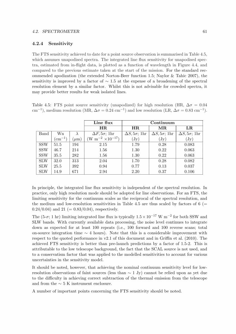
4.2. SPECTROMETER 61
4.2.4 Sensitivity
The FTS sensitivity achieved to date for a point source observation is summarised in Table 4.5,which assumes unapodised spectra. The integrated line flux sensitivity for unapodised spec-tra, estimated from in-flight data, is plotted as a function of wavelength in Figure 4.4, andcompared to the previous estimate taken at the start of the mission. For the standard rec-ommended apodization (the extended Norton-Beer function 1.5; Naylor & Tahic 2007), thesensitivity is improved by a factor of ∼ 1.5 at the expense of a broadening of the spectralresolution element by a similar factor. Whilst this is not advisable for crowded spectra, itmay provide better results for weak isolated lines.
Table 4.5: FTS point source sensitivity (unapodized) for high resolution (HR, ∆σ = 0.04cm−1), medium resolution (MR, ∆σ = 0.24 cm−1) and low resolution (LR, ∆σ = 0.83 cm−1).
Line flux ContinuumHR HR MR LR
Band Wn λ ∆F, 5σ; 1hr ∆S, 5σ; 1hr ∆S, 5σ; 1hr ∆S, 5σ; 1hr(cm−1) (µm) (W m−2 ×10⁻¹⁷) (Jy) (Jy) (Jy)
SSW 51.5 194 2.15 1.79 0.28 0.083SSW 46.7 214 1.56 1.30 0.22 0.063SSW 35.5 282 1.56 1.30 0.22 0.063
SLW 32.0 313 2.04 1.70 0.28 0.082SLW 25.5 392 0.94 0.77 0.13 0.037SLW 14.9 671 2.94 2.20 0.37 0.106
In principle, the integrated line flux sensitivity is independent of the spectral resolution. Inpractice, only high resolution mode should be adopted for line observations. For an FTS, thelimiting sensitivity for the continuum scales as the reciprocal of the spectral resolution, andthe medium and low-resolution sensitivities in Table 4.5 are thus scaled by factors of 6 (=0.24/0.04) and 21 (= 0.83/0.04), respectively.
The (5-σ; 1 hr) limiting integrated line flux is typically 1.5×10⁻¹⁷ W m−2 for both SSW andSLW bands. With currently available data processing, the noise level continues to integratedown as expected for at least 100 repeats (i.e., 100 forward and 100 reverse scans; totalon-source integration time ∼ 4 hours). Note that this is a considerable improvement withrespect to the quoted performance in v2.1 of this document and in Griffin et al. (2010). Theachieved FTS sensitivity is better than pre-launch predictions by a factor of 1.5-2. This isattributable to the low telescope background, the fact that the SCAL source is not used, andto a conservatism factor that was applied to the modelled sensitivities to account for variousuncertainties in the sensitivity model.
It should be noted, however, that achieving the nominal continuum sensitivity level for low-resolution observations of faint sources (less than ∼ 1 Jy) cannot be relied upon as yet dueto the difficulty in achieving correct subtraction of the thermal emission from the telescopeand from the ∼ 5 K instrument enclosure.
A number of important points concerning the FTS sensitivity should be noted.

62 CHAPTER 4. SPIRE IN-FLIGHT PERFORMANCE
Figure 4.4: FTS point source line flux sensitivity (unapodized) vs. wavenumber across theFTS bands. The current sensitivity (black line) is estimated from repeated observations ofdark sky and calibration objects, in comparison to the previous values (dashed grey line)estimated at the start of the mission.
1. The integrated line flux sensitivity for an unresolved line is in principle independentof the resolution for an FTS, so the high-resolution sensitivities also apply to mediumresolution mode. In practice the performance is better for high resolution mode, andthis is strongly recommended for sensitive line spectroscopy.
2. For point source observations, a sparse map covering the full FTS field of view is alsogenerated. The full field of view is 2.6 arcmin diameter, but the outer ring of detectorsis partially vignetted. The unvignetted field of view is specified as 2 arcmin. Data fromthe full field of view are available, but the accurate calibration of the outer parts cannotbe guaranteed at this time.
3. For very strong sources, a bright-source mode is available, for which the sensitivity isreduced compared to nominal mode by a factors of approximately 2 for the SLW arrayand 4 for the SSW array. Guidance on use of the bright source mode is provided inSection 5.3.4.
4. As for the photometer, the maximum achievable S/N should be taken as 200.
5. For spectral mapping:
(a) Integrated line flux sensitivity is essentially the same as for point source for a givenmap point (in terms of W m−2 in beam).
(b) For a fully sampled map, spatial pixels in the spectral cube can be co-added/resizedto enhance sensitivity (as in the photometer), but it is best to assume no enhance-

4.2. SPECTROMETER 63
ment in sensitivity as calibration errors or other imperfections may counteract thegain available in principle.
Continuum calibration should be cross-checked by including a map with the photometer inthe programme (this will generally occupy only a small fraction of the time for the FTSobservations).
4.2.5 Some HSpot Examples
Note that the observing overheads are much smaller than for any of the photometer modesas the telescope is not moved in the course of the observation.
High res Low res
Number of repeats 2 4 8 20 40On-source integration (s) 266 533 1066 256 512Instrument overheads (s) 236 239 246 272 312Observatory overheads (s) 180 180 180 180 180Total observation time (s) 682 952 1492 708 10041-σ noise (10−17 W m−2) (0.7-1.9) (0.5-1.4) (0.4-1.0) (30-80) mJy (21-56) mJy

64 CHAPTER 4. SPIRE IN-FLIGHT PERFORMANCE

Chapter 5
Flux Density Calibration
5.1 Calibration sources and models
SPIRE flux calibration is based on Neptune for the photometer and primarily on Uranusfor the spectrometer. The SPIRE calibration programme also includes observations of Mars,asteroids, and stars to enable a consistent and reliable flux calibration to be developed overthe course of the mission, and to ensure that cross calibration with PACS and HIFI, and withother facilities, is well established. The currently assumed asteroid and stellar models arebriefly described below for information.
5.1.1 Neptune and Uranus angular sizes and solid angles
The adopted equatorial radii (1-bar level) and eccentricities for Uranus and Neptune aresummarised in Table 5.1 and are based on the analysis of Voyager data by Lindal et al. (1987)and Lindal (1992). These are similar to the values used in the ground-based observations byGriffin & Orton (1993), Hildebrand et al. (1985) and Orton et al. (1986).
In calculating the planetary angular sizes and solid angles, a correction is applied for theinclination of the planet’s axis at the time of observation, and the apparent polar radius is
Table 5.1: Adopted planetary radii and eccentricity values.
Planet Equatorial radius Polar radius Eccentricity Referencereq (km) rp (km) Eq. (5.2)
Uranus 25, 559± 4 24, 973± 20 0.2129 Lindal et al. (1987)Neptune 24, 766± 15 24, 342± 30 0.1842 Lindal (1992)
Uranus 25,563 24,949 0.024 Griffin & Orton (1993)Neptune 24,760 24,240 0.021 Hildebrand et al. (1985)
Orton et al. (1986)
65

66 CHAPTER 5. FLUX DENSITY CALIBRATION
given by (Marth, 1897):
rp−a = req[1− e2 cos2 (φ)
]1/2, (5.1)
where φ is the latitude of the sub-Earth point, and e is the planet’s eccentricity:
e =
[r2eq − r2
p
r2eq
]1/2
. (5.2)
The observed planetary disc is taken to have a geometric mean radius, rgm, given by
rgm = (req.rp−a)1/2 . (5.3)
For a Herschel-planet distance of DH , the observed angular radius, θp, and solid angle, Ω, arethus
θp =rgmDH
and Ω = πθ2p. (5.4)
Typical angular radii for Uranus and Neptune are 1.7 arcsec and 1.1 arcsec respectively.
5.1.2 Neptune and Uranus models
Models of Uranus and Neptune by Moreno (1998, 2010) have been agreed by the HerschelCalibration Steering Group (HCalSG) as the current standards for Herschel, and are availableon the HCS calibration ftp site1. The Uranus and Neptune disk-averaged brightness temper-ature spectra are plotted in Figure 5.1. In the Herschel range, the disk averaged brightnesstemperatures increase with wavelength as deeper layers in the atmosphere are probed. Theplanets have similar temperatures, despite Neptune’s greater distance from the Sun, becauseNeptune has an internal heat source. This also leads to a more dynamic neptunian atmo-sphere resulting in some prominent spectral features whereas the Uranian spectrum is largelyfeatureless.
Typical photometer (250, 350, 500) µm calibration flux densities (see Section 5.2 for precisedefinition) are (160, 100, 60) Jy for Neptune and (370, 250, 150) Jy for Uranus.
The Uranus and Neptune models are currently quoted as accurate to ±5%. Note that themodels currently used for SPIRE are the “esa-2” tabulations. These may be subject tochange as knowledge of the atmospheric properties becomes more refined, based on Herscheland other observations. Any such changes will be assessed and authorised by the HCalSG, andcorresponding updates to the SPIRE and PACS flux calibration will be released accordingly.
5.1.3 Mars models
Web-based models of the martian continuum by Emmanuel Lellouch and Bryan Butler areavailable at http://www.lesia.obspm.fr/perso/emmanuel-lellouch/mars/ and http://
www.aoc.nrao.edu/~bbutler/work/mars/model/.
1ftp://ftp.sciops.esa.int/pub/hsc-calibration/

5.1. CALIBRATION SOURCES AND MODELS 67
Figure 5.1: Currently adopted models (Moreno, 2010) of the brightness temperature spectraof Uranus and Neptune.
Mars is a very bright source for SPIRE. For example, at the time of its observation by SPIREon OD 168 (29 Oct. 2009) it had flux densities of (9300, 5000, 2500) Jy at (250, 350, 500)µm. The nominal Herschel telescope background is equivalent to approximately (230, 250,270) Jy, so that Mars is equivalent to (40, 20, 10) time the nominal telescope brightness.
5.1.4 Asteroid models
The larger asteroids can also be used as FIR/submillimetre calibration sources, and wereparticularly important in the early part of the mission when Uranus and Neptune were notvisible. The most accurate asteroid models are the thermophysical models of Muller & Lager-ros (2002), which have been tabulated by Muller (2009) and must be computed in detail for agiven observation date and time (there can be significant variations in brightness associatedwith the asteroid rotation period). For planning and estimation purposes, the asteroid Stan-dard Thermal Model (STM) (Lebofsky et al., 1986) can be used to estimate the expected fluxdensities.
As an illustration, STM spectra for Dec. 9 2009 are shown in Figure 5.2 for the four largestasteroids, 1-Ceres, 2-Pallas, 3-Juno, and 4-Vesta. Note that STM asteroid spectra are all ofapproximately the same shape, close to that of a Rayleigh-Jeans black body: the monochro-matic flux density ratios are typically 1.98 for S350/S500 and 3.7–3.8 for S250/S500.
The initial SPIRE photometer flux calibration was based on observations of 1-Ceres on OD50(02 July 2009), for which the Ceres thermal spectrum was derived using the STM. This initialcalibration has now been superseded by the Neptune-based calibration. The changes to the

68 CHAPTER 5. FLUX DENSITY CALIBRATION
flux calibration scale are quite small, but the uncertainties are now much improved2.
Figure 5.2: Standard Thermal Model spectra of 1-Ceres, 2-Pallas, 3-Juno, and 4-Vesta forDec. 9 2009.
5.1.5 Stellar calibrators
At present, the PACS photometer calibration is based on a set of standard stars identifiedby the HCalSG. These stars are also being observed by SPIRE as part of the SPIRE-PACScross calibration programme, which will include detailed comparison of the stellar-based andNeptune-based calibrations. The eight stars are: α Boo, α Tau, γ And, β Peg, γ Dra, Sirius,and α Cet.
Model spectra for these stars have been generated by Leen Decin based on the MARCS stellaratmosphere code of Decin & Eriksson (2007), covering 2-200 µm, and the data are availablefrom within the Herschel Interactive Processing Environment3. The quoted estimated uncer-tainty is 1% for that wavelength range. Figure 5.3 shows the model FIR SEDs for the eightstellar calibrators with extrapolations to the SPIRE photometer bands based on the spectralindex in the 150-200 µm range. The latter is fairly uniform, varying between −1.99 and−2.034 for the eight sources. Computations covering wavelengths up to 700 µm are awaited.In the meantime, the available SEDs can be extrapolated with reasonable accuracy to SPIREwavelengths, assuming no excess emission due to a chromospheric component or to a colddust component around the star. The presence of any such excess would lead to a higher fluxdensity, so the extrapolated figures can be taken as lower limits.
2Note that the small correction factors to the flux calibration scale (1.02, 1.05, 0.94 for 250, 350, 500 µmrespectively) announced in the SPIRE Scan-Map AOT Release Note (Issue 2, Oct. 21 2009) are no longerneeded for data processed using SPIRE Calibration Tree v5.0 and above, and should not be applied.
3The calibration source database, Calsdb, documentation is available from the HSC web pages

5.2. PHOTOMETER FLUX CALIBRATION SCHEME 69
Figure 5.3: Decin & Eriksson (2007) FIR SEDs model for the eight stellar calibrators withextrapolations to the SPIRE photometer bands.
5.2 Photometer flux calibration scheme
The photometer pipeline produces monochromatic in-beam flux densities (Jy/beam) at stan-dard frequencies corresponding to 250, 350 and 500 µm, and calculated under the assumptionsof (i) a point source observation and (ii) a flat νSν spectrum. The calibration is carried outat the level of the detector timelines (Level-1 data products). The SPIRE Level-2 photometerproducts (maps) are also calibrated in terms of in-beam flux density (Jy/beam) rather thansurface brightness (Jy/pixel or /sr).
The primary calibration standard is Neptune (Moreno 2010 model) which has an estimatedabsolute uncertainty of 5%. The detailed computations, and the appropriate corrections foran extended source or to convert to a different assumed source spectrum, are described inthis section.
5.2.1 Photometer Relative Spectral Response Function
In a SPIRE photometer observation, the property of the source that is directly proportional tosource power absorbed by the bolometer is the integral over the passband of the flux density

70 CHAPTER 5. FLUX DENSITY CALIBRATION
weighted by the instrument Relative Spectral Response Function (RSRF), as indicated inFigure 5.4:
SS =
∫Passband
SS(ν)R(ν) dν∫Passband
R(ν) dν, (5.5)
where SS(ν) represents the in-beam source flux density at the telescope aperture and R(ν) isthe RSRF.
Figure 5.4: RSRF-weighted flux density defined as the integral of the source spectrumweighted by the instrument RSRF
The three photometer RSRFs are shown in Figure 5.5. The thick lines correspond to theoverall filter transmission functions, and give the RSRFs, RP (ν), for the case of a point source.The thin lines are the RSRFs for an extended source, RE(ν). An extended source is definedhere as a source that fills the entire beam solid angle with a uniform surface brightness4.The extended source profiles are derived by weighting the point source RSRFs by λ2 to takeinto account the single-mode coupling via the feedhorns. This λ2 weighting effectively takesinto account the fact that the beam width varies across the band in proportion to λ, leadingto a larger beam area at longer wavelengths and so additional power coupled from extendedemission. Note that the absolute vertical scale in Figure 5.5 is irrelevant to the computationsin this note as all relevant parameters involve ratios of RSRF integrals. The RSRF curvescan be accessed from the SPIRE Calibration Tree in the Herschel Interactive ProcessingEnvironment (HIPE) and also from the HSC ftp.5
5.2.2 Calibration flux densities
Let the RSRF for a point source observation be RP (ν) and that for an extended source beRE(ν) (as shown in Figure 5.5, right). The standard calibration source, Neptune, is small(diameter < 2.5 arcsec) compared to the SPIRE beam widths, so RP (ν) is the appropriateRSRF.
4The accurate calibration of a source which is semi-extended with respect to the beam depends on the exactdetails of the surface brightness distribution, and is beyond the scope of this document.
5Available at ftp://ftp.sciops.esa.int/pub/hsc-calibration/SPIRE/PHOT/Filters/

5.2. PHOTOMETER FLUX CALIBRATION SCHEME 71
Figure 5.5: Photometer RSRFs: RP (ν) (thick lines; point source; no weighting of filtertransmission profiles) RE(ν) (thin lines; extended source; λ2 weighting). The wavelengthscale on the top is given for reference.
When observing a calibration source, the property that is directly proportional to absorbeddetector power is
SCalib = KBeam
∫Passband
SC(ν)RP (ν) dν∫Passband
RP (ν) dν, (5.6)
where SC is the calibrator flux density at the telescope aperture and KBeam is a correctionfactor for partial resolution of the calibrator by the telescope beam. For a Gaussian beamprofile coupling to a uniformly bright disk (planet or asteroid), the beam correction factor isgiven by (Ulich & Haas, 1976):
KBeam(θp, θBeam) =1− exp(−x)
x; x = 4 ln (2)
(θp
θBeam
)2
, (5.7)
where θp is the angular radius of the disk, and θBeam is the beam FWHM. The corresponding(250, 350, 500) µm beam correction factors are small: (0.988, 0.994, 0.997) for Uranus and(0.995, 0.997, 0.999) for Neptune.

72 CHAPTER 5. FLUX DENSITY CALIBRATION
SCalib for Neptune has been used in the derivation of the flux density conversion moduleparameters that are applied in the pipeline, and which are in turn used to derive the RSRF-weighted source flux density SS .
5.2.3 Response of a SPIRE bolometer to incident power
The output signal voltage of a SPIRE bolometer depends on the absorbed signal power, whichis in turn a function of the source power collected by the telescope. For NTD bolometers witha given applied bias voltage, the small-signal responsivity varies with the voltage across thebolometer with an approximately linear relationship over a wide range of background loadingand bath temperature conditions. This translates to a corresponding relationship for thedifferential sensitivity of the system to the RSRF-weighted flux density, S:
dV
dQ∝ V =>
dV
dS∝ V (5.8)
To allow for the fact that the responsivity-operating point voltage relationship will not beexactly linear, we let
dS
dV= f(V ). (5.9)
Note that:
1. f(V ) is specific to a particular bolometer and bias setting;
2. f(V ) is negative (since absorbed power causes a decrease in bolometer voltage); however,in the rest of this document we take it to be positive for convenience, assuming that acorrection factor of −1 is applied.
In order to perform conveniently the integration of f(V ), an appropriate function can befitted to it. Various fitting functions have been investigated and it is found that the mostsuitable function is of the form:
f(V ) = K1 +K2
V −K3, (5.10)
where K1, K2 and K3 are constants. K1 has units of Jy V−1, K2 has units of Jy, and K3 hasunits of V.
An example plot of f(V ) vs. V is shown Figure 5.6, and corresponds to a typical SPIRE 350µm bolometer. The nominal operating point (blank sky) in this case would be close to 3 mV,and the range covered by the plot covers a sky brightness range up to more than 10 times thetelescope brightness. The blue points are derived from a bolometer model, and the red linecorresponds to the best fit K-parameters using equation 5.10.

5.2. PHOTOMETER FLUX CALIBRATION SCHEME 73
Figure 5.6: Typical plot of f(V ) vs. V (for a nominal 350 µm bolometer). The blue pointscorrespond to the bolometer model and the red line is the fitted function using equation 5.10.
A flux density corresponding to a measured RMS bolometer voltage, Vm, can be derived byintegrating the above expression between some fixed bolometer voltage, V0, and Vm:
S =
Vm∫V0
f(V )dV =
Vm∫V0
(K1 +
K2
V −K3
)dV, (5.11)
so
S = K1(Vm − V0) +K2 ln
(Vm −K3
V0 −K3
). (5.12)
Ideally, V0 would be the bolometer voltage in the absence of any astronomical signal (i.e.,what would be measured when observing blank sky in otherwise identical conditions). Theresulting flux density would correspond to that from the sky calibrated with respect to theblank sky level. V0 is therefore derived from standard calibration observations of a “dark”area of sky in scan-map mode under the nominal conditions: bias voltage and frequency,bolometer and instrument FPU (Level-1) temperature, and telescope temperature. Ideallythe conditions would be the same for the calibration and science observations but smalldifferences are inevitable in practice. V0 thus differs from the ideal value (by an amountmuch larger than most astronomical signals). This means that the raw flux density valuesproduced by the pipeline have additive offsets (different for each bolometer) that must beremoved before map-making to derive the flux density from the sky.
Values of K1, K2 and K3 have been derived from calibration observations, and are used in thepipeline flux conversion module together with the K4P parameter (see the next subsection)to produce the SPIRE flux density timelines.

74 CHAPTER 5. FLUX DENSITY CALIBRATION
5.2.4 Conversion of RSRF-weighted flux density to monochromatic fluxdensity
Definition of a monochromatic flux density requires the adoption of a standard frequencyfor the band and some assumption about the shape of the source spectrum. The approachadopted for SPIRE and PACS is to assume that the spectrum is a power law across the banddefined by the flux density at a standard frequency ν0 , and a spectral index αS :
SS(ν) = SS(ν0)
(ν
ν0
)αS
. (5.13)
The convention adopted for Herschel is to adopt αS = αS0 = −1 (corresponding to ν Sν flatacross the band). For SPIRE, we choose values of ν0 to correspond to wavelengths of 250,350 and 500 µm for the three bands, and monochromatic flux densities at those frequenciesare generated by the pipeline.
Under this assumption, the measured RSRF-weighted flux density (to which the bolometeroutput voltage due to the source is proportional in the linear regime) is thus
SS =SS(ν0)
ναS0
∫
Passband
ναSR(ν)dν∫Passband
R(ν)dν
, (5.14)
where R(ν) = RP (ν) for a point source or RE(ν) for an extended source.
The source flux density at frequency ν0, which is produced by the pipeline, is therefore givenby:
SS(ν0) = SS
ναS0
∫Passband
R(ν)dν∫Passband
ναS R(ν)dν
= K4 SS . (5.15)
The measured RSRF-weighted flux density is thus multiplied by K4 to derive the monochro-matic flux density at the standard wavelength to be quoted to the user.
Putting αS = −1 gives
K4 =1
ν0
∫Passband
R(ν)dν∫Passband
R(ν)ν dν
. (5.16)
Note that the values of K4 are different for point and extended sources:
K4P =1
ν0
∫Passband
RP (ν)dν∫Passband
RP (ν)ν dν
. (5.17)

5.2. PHOTOMETER FLUX CALIBRATION SCHEME 75
and
K4E =1
ν0
∫Passband
RE(ν)dν∫Passband
RE(ν)ν dν
. (5.18)
The SPIRE photometer pipeline is based on the point source case and so uses K4P in thevoltage-to-flux density conversion. To derive the flux density for an extended source, thepipeline output must be multiplied by K4E/K4P . In addition, a colour correction is usuallyrequired, the procedure for which is given in Sections 5.2.5 and 5.2.9.
5.2.5 Colour correction
The assumption that the source has a spectrum with ν Sν flat across the band (αS0 = −1)will not be the case for most observations. For instance, at SPIRE wavelengths, planetsand other solar system objects will typically have a spectral index of 2 (corresponding toblack body emission in the Rayleigh-Jeans region). Dust sources will typically have a steeperspectrum, with αS0 = 3− 4. For the highest calibration accuracy a colour correction can beapplied by the astronomer based on other information (for instance, measurements in otherSPIRE or PACS bands and/or data from other telescopes). Depending on the nature andtemperature of the source, the true spectral index could be different for the three SPIREbands, as illustrated in Figure 5.7, which could apply in the case of a cold dust source.
Figure 5.7: Illustration of the possibility of different source spectral indices for the threeSPIRE bands.
Given the width of the SPIRE bands and the nature of the observed source SEDs, in mostcases it will be appropriate to assume that the source spectrum follows a power law acrossthe band, but with a different spectral index, αSnew. Let S′S(ν0) be the source flux density

76 CHAPTER 5. FLUX DENSITY CALIBRATION
at ν0 for that spectral shape. We then have from equation 5.15
S′S(ν0) = ν(αSnew−αS0)
∫
Passband
R(ν)ναS0 dν∫Passband
R(ν)ναSnew dν
SS(ν0) = KC(αSnew)SS(ν0). (5.19)
Putting αS0 = −1 gives
KC(αSnew) = ν(αSnew+1)0
∫
Passband
R(ν)ν−1 dν∫Passband
R(ν)ναSnew dν
. (5.20)
Once again, KC is different for point and extended sources due to the different RSRFs. Thecolour correction factors for SPIRE are given in Section 5.2.8, and an example of how to applythe colour correction is given in Section 5.2.9.
5.2.6 Conversion of in-beam flux density to surface brightness
The in-beam astronomical flux density at a given frequency, ν, is defined as:
S(ν) =
∮4π
B(θ, φ) Iν(θ, φ) dΩ, (5.21)
where θ ∈ [0, π] is a radial angular offset from the beam centre, φ ∈ [0, 2π] is an azimuthalangular offset, B(θ, φ) is the normalised beam profile, Iν(θ, φ) is the sky intensity (surfacebrightness) profile, and dΩ is a solid angle element in the direction defined by (θ, φ). Notethat we assume here that the beam profile can be regarded as uniform across the spectralpassband (the effect of beam profile variation across the band is taken into account by theextended source RSRF, as described in Section 5.2.1).
The pipeline produced flux densities in terms of Jy in-beam. For an extended sources whichis uniformly bright over the beam area (solid angle), the surface brightness (Jy arcsec−2 orJy sr−1) can be obtained from the flux density by dividing it by the beam area.
The beam area is
ABeam =
∮4π
B(θ, φ) dΩ. (5.22)
For a Gaussian beam profile with FWHM θBeam, the beam area is given by
ABeam =πθ2
Beam
4 ln (2). (5.23)
However, the SPIRE beams exhibit departures from Gaussianity at low levels due to thediffraction effects of the central obscuration and the secondary supports, and it is importantto use the full beam area in the conversion, as explained in Section 5.2.7

5.2. PHOTOMETER FLUX CALIBRATION SCHEME 77
5.2.7 Photometer beam maps and areas
Updated SPIRE photometer beam data and accompanying detailed information are availableat the HSC calibration ftp site6 and comprise the following:
• new empirical beam maps based on fine-scan-map measurements of Neptune;
• the raw data used for the above;
• a theoretical model including coverage of the sidelobes and low-level structure due tothe secondary mirror supports (unchanged from the previous issue);
• a technical note (SPIRE Beam Model Release Note, version 1.0a) providing detailedinformation on the beam maps and parameters and how they were derived
Empirical beam maps
The empirical beam products consist of two sets of three beam maps, one for each photometerband. The product is derived from scan-map data of Neptune, performed using a custom“fine-scan” observing mode with the nominal source brightness setting. In these fine-scanobservations, each bolometer is scanned over Neptune in four different directions. The datawere reduced using the standard HIPE scan-map pipeline and the naıve map-maker. Eachmap constitutes an averaging in the map over all of the individual bolometers crossing thesource, and represents the realistic point source response function of the system, including allscanning artefacts. It is worth noting that in a normal SPIRE scan-map, any individual sourcein the map will be covered by only a subset of bolometers, leading to low-level beam profilevariations, from position to position in the map, about the average profile presented here.These beam products also represent the measurement of a source with a ν2 spectral shape.A source with a different spectral shape will produce a slightly different beam parameters.
The beam maps for all three bands are displayed in log scaling in Figure 5.8. Four individualmaps, one from each of the four observations from which the final beam products are derived,are also available should the user want to investigate the beam stability. The beam productmaps are ∼ 10×30 arcmin in scale and include the same extensions and header information asthe nominal maps output from HIPE. There are two versions of each map, one high resolutionwith a 1 arcsec pixel scale, and another with the nominal SPIRE output map pixel scale of(6, 10, 14) arcsec per pixel for (250, 350, 500) µm. The data have also been normalised togive a peak flux of unity in all three bands.
Note that the ellipticity seen in the maps is not a function of scanning direction, but is constantwith position angle. When using these beam models it is advised that the user rotates thebeam map so that it matches the position angle of the user’s data. The position angle of HIPEmaps can be found in the primary FITS header and is specified by the posangle keyword.
Table 5.2 summarises the basic beam parameters for data binned into 1 arcsec map pixels.The FWHM values are determined by fitting an asymmetric 2-D Gaussian to the beam maps,and the beam areas are computed by integrating explicitly under the measured beam profiles.The basic beam parameters vary as a function of pixel scale, with the FWHM values and beam
6ftp://ftp.sciops.esa.int/pub/hsc-calibration/SPIRE/Beams

78 CHAPTER 5. FLUX DENSITY CALIBRATION
Figure 5.8: Log scale images for the empirical SPIRE beam model at 250, 350, and 500 µmfrom left to right respectively. The top row uses a 1 arcsec pixel scale for all maps, and thebottom row uses the nominal SPIRE map pixel scales of 6, 10, and 14 arcsec from left toright respectively.
areas increasing with pixel size (see Table 4.1 in Chapter 4). This is expected since the fidelityof the surface brightness reconstruction becomes less reliable at low resolution, particularlywith respect to the Airy ring pattern at higher radii from the source peak. For example, theexplicit integration under the measured beams in standard maps with (6,10,14) arcsec pixelsproduces beam areas of (447,816,1711) arcsec2, which are larger, by factors of approximately(1.35, 1.31, 1.27) at (250, 350, 500) µm, than those derived from higher resolution beam scans(maps with 1 arcsec/pixel). Consequently, we recommend to use the as-measured beam areain 1 arcsec maps in the flux-density to surface brightness conversion.
Raw empirical data
This product is the raw data set from which the empirical beam maps were derived. It hasbeen made available so that users who wish to apply a custom data processing steps can alsoapply this processing to the beam model data, thereby obtaining a model representative ofthe beam within their reduced maps.

5.2. PHOTOMETER FLUX CALIBRATION SCHEME 79
Table 5.2: Basic 2-D Gaussian parameters for measured beams on maps with a 1 arcsec pixelsize. Uncertainties in the beam FWHM values and areas are estimated at < 1%.
Band Major×Minor-FWHM
GeometricmeanFWHM
Ellip-ticity
Average beam area
(µm) (arcsec) (arcsec) (%) (arcsec)2 (sr ×10−8)
250 18.3× 17.0 17.6 8.1 423 0.9942350 24.7× 23.2 23.9 6.6 751 1.765500 37.0× 33.4 35.2 10.9 1587 3.730
Optical model of photometer beams
The theoretical model of the beams is based on an optical model of the telescope and the in-strument, which has been shown by analysis of in-flight data to provide a highly representativecharacterisation of the low-level structure in the beams. The model is based on computationsof the response function of the end-to-end optical train of the Herschel observatory and SPIREphotometer at individual in-band wavelengths, then summing the monochromatic responsewith specific weights. The model contains the reconstructed wave-front error distribution ofthe telescope taken from ground measurements, taking into account the dominant impact ofthe flight environmental conditions (gravity release, cryo-vacuum operation), as well as thedetailed pupil obscuration from the full observatory geometry. The full SPIRE instrumentoptical model including the entire photometer train up to focal plane is also implemented (seeFigure 5.9). The simulated source is a coherent point source with continuum Rayleigh-Jeans(RJ) spectrum, representative of most bright point sources with brightness temperature. Theeffect of the detector feedhorn is taken into account by including further pupil apodisationwith a spectrally-varying edge taper (and associated spectral shift of the diffraction focus)within each band, which has been characterised during SPIRE ground calibration.
The full band response is obtained by spectral weighting of the set of individual responses. Theweights are obtained by product of the Rayleigh-Jeans source spectrum with the instrumentRelative Spectral Response Function (RSRF) in each band, the spectral in-band throughputAΩ and finally the spectral in-band coupling, all derived from flight model instrument levelground calibration.
The derived beam models can be considered as “static” noise-free point source reference maps,complementary to the empirical maps which, being flight measured and pipeline generated,include the additional effects among others of electronics detection, scanning, processing andmap reconstruction and general additional background noise from sky and observatory.
Figure 5.10 shows the theoretical beam models, all given at a 0.6 arcsec sampling over a 6×6arcmin angular extent and in the spacecraft coordinate system (Y/Z; rotation via the user’sdefined position angle will transfer into the relevant sky coordinate systems).
The model beam product provides significantly higher detail at greater radius but presentlyis released only at 6 × 6 arcmin scale. Larger scale beam models (e.g., up to 1 deg scale) atlower sampling (e.g. standard 6, 10, 14 arcsec) have been generated in order to provide better

80 CHAPTER 5. FLUX DENSITY CALIBRATION
Figure 5.9: View of the model geometry (left) and reconstructed telescope pupil optical pathdifference map from environmental ground measurements by Herschel Observatory industrialcontractors (right).
estimates on integrated beam extent/effective surface area and may be released later.
5.2.8 Computed conversion factors for SPIRE
Factor K4 to convert RSRF-weighted flux density to monochromatic flux density
For the standard spectral index of αS0 = −1 adopted for Herschel, the values of K4 (ascomputed using equations 5.17 and 5.18) for the three SPIRE bands are:
Point source (no RSRF weighting):K4P (250, 350, 500) µm = (1.0113, 1.0087, 1.0065).
Extended source (λ2 RSRF weighting):K4E (250, 350, 500) µm = (0.9939, 0.9920, 0.9773).
The conversion factors from point source calibration (SPIRE pipeline convention) to extendedsource calibration are thus:K4E/K4P (250, 350, 500) µm = (0.9828, 0.9834, 0.9710).
Level-1 or Level-2 (see Chapter 6) data must be multiplied by these values to convert frompoint source to extended source calibration.
Note that at the time of writing the latest version of the SPIRE Calibration Tree is v7.0. Ifone is using data processed with v5.0, then there is no immediate need to re-run the pipeline.A simple multiplicative factor of 1.0067 can be applied to the PMW pipeline output to achievean equivalent calibration to v7.0.
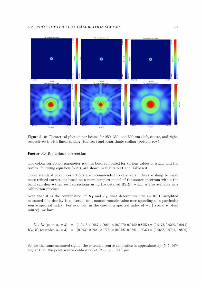
5.2. PHOTOMETER FLUX CALIBRATION SCHEME 81
Figure 5.10: Theoretical photometer beams for 250, 350, and 500 µm (left, centre, and right,respectively), with linear scaling (top row) and logarithmic scaling (bottom row)
Factor KC for colour correction
The colour correction parameter KC has been computed for various values of αSnew and theresults, following equation (5.20), are shown in Figure 5.11 and Table 5.3.
These standard colour corrections are recommended to observers. Users wishing to makemore refined corrections based on a more complex model of the source spectrum within theband can derive their own corrections using the detailed RSRF, which is also available as acalibration product.
Note that it is the combination of K4 and KC that determines how an RSRF-weightedmeasured flux density is converted to a monochromatic value corresponding to a particularsource spectral index. For example, in the case of a spectral index of +3 (typical ν3 dustsource), we have:
K4P KC(point, αs = 3) = (1.0113, 1.0087, 1.0065)× (0.9070, 0.9180, 0.8952) = (0.9173, 0.9260, 0.9011)
K4E KC(extended, αs = 3) = (0.9939, 0.9920, 0.9773)× (0.9727, 0.9821, 1.0037) = (0.9668, 0.9742, 0.9809).
So, for the same measured signal, the extended source calibration is approximately (5, 5, 9)%higher than the point source calibration at (250, 350, 500) µm.
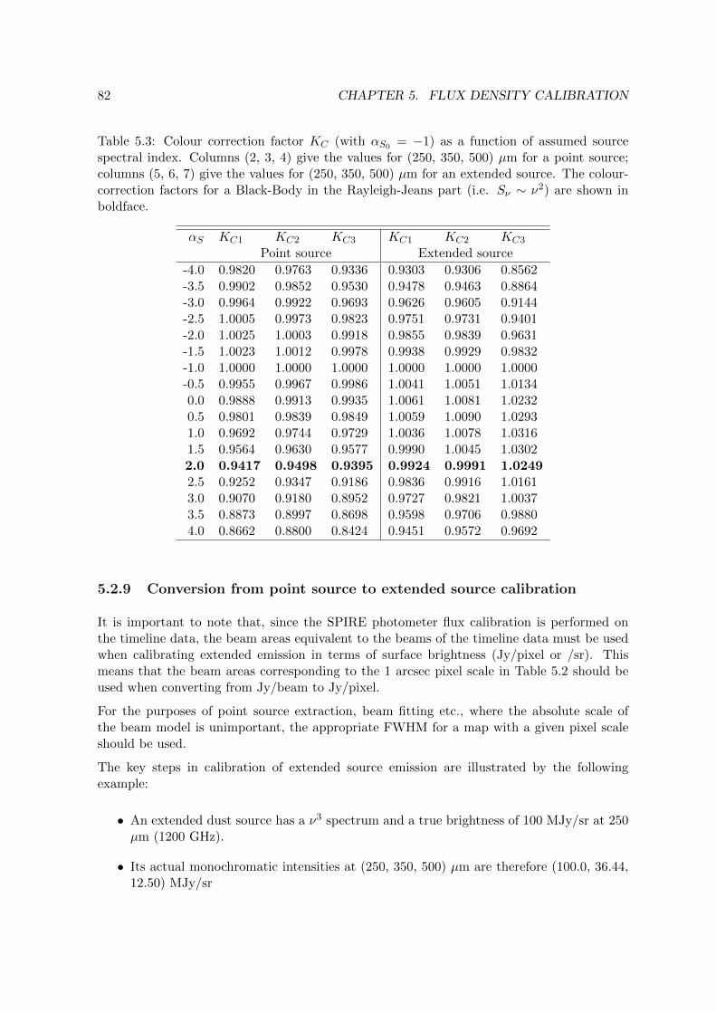
82 CHAPTER 5. FLUX DENSITY CALIBRATION
Table 5.3: Colour correction factor KC (with αS0 = −1) as a function of assumed sourcespectral index. Columns (2, 3, 4) give the values for (250, 350, 500) µm for a point source;columns (5, 6, 7) give the values for (250, 350, 500) µm for an extended source. The colour-correction factors for a Black-Body in the Rayleigh-Jeans part (i.e. Sν ∼ ν2) are shown inboldface.
αS KC1 KC2 KC3 KC1 KC2 KC3
Point source Extended source
-4.0 0.9820 0.9763 0.9336 0.9303 0.9306 0.8562-3.5 0.9902 0.9852 0.9530 0.9478 0.9463 0.8864-3.0 0.9964 0.9922 0.9693 0.9626 0.9605 0.9144-2.5 1.0005 0.9973 0.9823 0.9751 0.9731 0.9401-2.0 1.0025 1.0003 0.9918 0.9855 0.9839 0.9631-1.5 1.0023 1.0012 0.9978 0.9938 0.9929 0.9832-1.0 1.0000 1.0000 1.0000 1.0000 1.0000 1.0000-0.5 0.9955 0.9967 0.9986 1.0041 1.0051 1.01340.0 0.9888 0.9913 0.9935 1.0061 1.0081 1.02320.5 0.9801 0.9839 0.9849 1.0059 1.0090 1.02931.0 0.9692 0.9744 0.9729 1.0036 1.0078 1.03161.5 0.9564 0.9630 0.9577 0.9990 1.0045 1.03022.0 0.9417 0.9498 0.9395 0.9924 0.9991 1.02492.5 0.9252 0.9347 0.9186 0.9836 0.9916 1.01613.0 0.9070 0.9180 0.8952 0.9727 0.9821 1.00373.5 0.8873 0.8997 0.8698 0.9598 0.9706 0.98804.0 0.8662 0.8800 0.8424 0.9451 0.9572 0.9692
5.2.9 Conversion from point source to extended source calibration
It is important to note that, since the SPIRE photometer flux calibration is performed onthe timeline data, the beam areas equivalent to the beams of the timeline data must be usedwhen calibrating extended emission in terms of surface brightness (Jy/pixel or /sr). Thismeans that the beam areas corresponding to the 1 arcsec pixel scale in Table 5.2 should beused when converting from Jy/beam to Jy/pixel.
For the purposes of point source extraction, beam fitting etc., where the absolute scale ofthe beam model is unimportant, the appropriate FWHM for a map with a given pixel scaleshould be used.
The key steps in calibration of extended source emission are illustrated by the followingexample:
• An extended dust source has a ν3 spectrum and a true brightness of 100 MJy/sr at 250µm (1200 GHz).
• Its actual monochromatic intensities at (250, 350, 500) µm are therefore (100.0, 36.44,12.50) MJy/sr
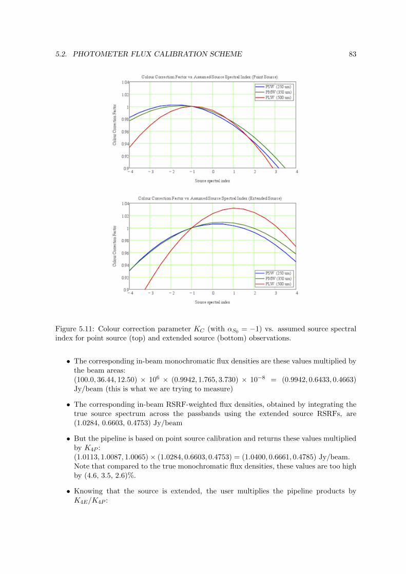
5.2. PHOTOMETER FLUX CALIBRATION SCHEME 83
Figure 5.11: Colour correction parameter KC (with αS0 = −1) vs. assumed source spectralindex for point source (top) and extended source (bottom) observations.
• The corresponding in-beam monochromatic flux densities are these values multiplied bythe beam areas:(100.0, 36.44, 12.50) × 106 × (0.9942, 1.765, 3.730) × 10−8 = (0.9942, 0.6433, 0.4663)Jy/beam (this is what we are trying to measure)
• The corresponding in-beam RSRF-weighted flux densities, obtained by integrating thetrue source spectrum across the passbands using the extended source RSRFs, are(1.0284, 0.6603, 0.4753) Jy/beam
• But the pipeline is based on point source calibration and returns these values multipliedby K4P :(1.0113, 1.0087, 1.0065)× (1.0284, 0.6603, 0.4753) = (1.0400, 0.6661, 0.4785) Jy/beam.Note that compared to the true monochromatic flux densities, these values are too highby (4.6, 3.5, 2.6)%.
• Knowing that the source is extended, the user multiplies the pipeline products byK4E/K4P :

84 CHAPTER 5. FLUX DENSITY CALIBRATION
(1.0400, 0.6661, 0.4785)× (0.9828, 0.9834, 0.9710) = (1.0221, 0.6550, 0.4646) Jy/beamNote that these values are rather more accurate – high by only (+2.8, +1.8, −0.4)%with respect to the true monochromatic flux densities, but are still based on an assumedν−1 spectrum.
• Knowing also that the source has a ν3 spectrum, not ν−1 as assumed in the pipeline, theuser applies the appropriate extended source colour correction factors from Table 5.3 toobtain the true in-beam monochromatic flux densities:(0.9727, 0.9821, 1.0037)× (1.0221, 0.6550, 0.4646) = (0.9942, 0.6433, 0.4663) Jy/beam
• What if, inappropriately, the point source calibration is left unchanged and the pointsource colour correction applied?(0.9070, 0.9180, 0.8952)× (1.0400, 0.6661, 0.4785) = (0.9433, 0.6115, 0.4283) Jy/beami.e., the resulting flux densities are too low by (5.2, 5.4, 8.9)% at (250, 350, 500) µm.
5.2.10 Photometer calibration accuracy
SPIRE photometer observations are subject to several kinds of uncertainty.
Absolute calibration uncertainty: This component is associated with our knowledge ofthe brightness of the primary calibrator, Neptune, and is estimated at ±5%. It is corre-lated across the three bands, i.e., flux densities in the three bands will move up or downsystematically in the event of this calibration being revised.
Relative calibration uncertainty: This uncertainty arises from the process of comparinga source observation with Neptune (using the Neptune-derived voltage to flux density pa-rameters that are implemented in the pipeline). This is a random contribution and has beenestimated by careful analysis of repeated measurements of a bright source (actually Neptuneitself). The results show that this component is less than 2% in all bands.
At present, we recommend that the overall calibration uncertainty for the SPIRE photometer,taking these two contributions into account, should be taken conservatively as ±7% (the directrather than quadrature sum of the absolute and relative calibration uncertainties). It shouldbe noted that this is dominated by the absolute component and is thus largely correlatedacross the three bands.
Photometric uncertainty: This component is due to the source measurement errors. Thephotometer pipeline produces timelines representing the the in-beam flux density, and somerandom detector noise will be present in the timelines. Any astrometric errors will alsointroduce additional noise when timelines are combined in mapmaking. In addition, in order toderive estimates of, for example, the flux density of a point or compact source, users will needto employ some suitable fitting or aperture photometry technique, and additional uncertaintiescan be introduced due to confusion or source crowding. In addition, slight differences in thechoice of pipeline parameters (e.g., for the deglitching and baseline subtraction modules) mayproduce slightly different results (at the level of a few percent).
It is important to note that these photometric uncertainties will be significant or dominantexcept for sources which stand out very clearly above any confusion noise or local sky back-ground fluctuations (in which case the calibration uncertainties described above will become

5.2. PHOTOMETER FLUX CALIBRATION SCHEME 85
significant or dominant). Assessment of the photometric uncertainties will depend on the par-ticular sky brightness distribution and on the source extraction or background subtractionmethods, and is is therefore something to be done carefully by the user.
See Section 5.2.11 for some additional considerations relating to the process of point sourceextraction.
5.2.11 A note on point source extraction from SPIRE Level-2 maps
The SPIRE flux calibration is time-line based (Jy in beam). As a result, the signal level ina map pixel depends on how the square map pixel size compares to the size of the beam.Only in the limit of infinitely small map pixels would a pixel co-aligned with a point sourceregister the true source flux density. It is important to note that no pixel size correctionfactors are incorporated in the SPIRE Level-2 map-making. For a given map pixel, theflux density value represents the average in-beam flux density measured by thedetectors while pointed within that area. Taking the pixel value for the flux density of anisolated co-aligned point source in an otherwise blank map would thus yield an underestimateof the true flux density.
The necessary correction factor is a function of the map pixel size and the beam size, and isa simple multiplicative factor. For a symmetrical Gaussian beam of FWHM θBeam, a squarepixel of side θPix, and a co-aligned source, the correction factor is:
P =π
4 ln(2)
(θBeam
θPix
)2
erf2
[(θPix
θBeam
)[ln(2)]1/2
], (5.24)
where erf is the error function erf(x) = 2π
∫ x0 e−t2 dt.
However, in the general case the source will be randomly aligned with respect to the map pixelresulting in a slightly different correction, and a small random uncertainty corresponding tothe actual offset of the source with respect to the pixel centre for a particular observation.Moreover, the source is not completely covered on infinitesimal scales; the beams are onlysampled along the locations where the detectors crossed over the beam.
Tests of how the measured flux density of point sources in map data have been performed usingstandard large and small scan map observations of Neptune (for 500 µm only) and γ Dra (forall three bands) to test the pixelisation corrections given by Equation 5.24. Maps from thesedata were generated at various pixel scales, the data were fitted with Gaussian functions,and then the resulting median flux densities (in the case of the γ Dra data) or medianmeasured/model flux density ratios (in the case of Neptune) were examined to understandhow the measured flux densities vary as a function of pixel size.
For 250 µm data, these tests demonstrated that Equation 5.24 provides an accurate correctionfor point source flux densities measured by PSF fitting in maps in all situations. For 350 µmdata, these tests demonstrated that Equation 5.24 provides an accurate correction for pointsource flux densities measured by PSF fitting in maps for only sources at the centres of smallscan maps. The results from the 350 µm large scan map data indicate that the measured fluxdensities may be lower (by a few percent) than what is implied by Equation 5.24 if the sourceis not centered within scan legs, although the exact decrease in flux density depends on thelocation of the source relative to the scan legs. For 500 µm, we found that Equation 5.24 did

86 CHAPTER 5. FLUX DENSITY CALIBRATION
not provide an accurate correction. Instead, the following empirical equation should be used:
P = 1− 0.0018 θPix − 0.00037 θ2Pix, (5.25)
where θPix is the pixel size in arcsec.
Performing the pixelisation correction introduces an additional uncertainty which is best todetermine empirically. At this time, this has only been characterized for 500 µm maps. Thefractional uncertainty due to the pixelisation correction is given by
UP = 0.0023− 0.00113 θPix. (5.26)
The default HIPE pixel sizes for (250, 350, 500) µm are θPix = (6, 10, 14) arcsec. Thecorresponding pixel size correction factors, given by Equations 5.24 and 5.25, are P =(0.951, 0.931, 0.902). From Equation 5.26, the corresponding percentage uncertainties in-troduced into the point source flux density estimation at 500 µm is 1.5%. This uncertaintyshould be added in quadrature to the other statistical uncertainties of the measurement. Notethat similar uncertainties may be appropriate to apply to 250 and 350 µm data but have notyet been derived.
The pixelisation corrections presented here have been derived for and tested on images createdby the naive mapmaker incorporated within HIPE, which uses a nearest-neighbour mappingalgorithm. Other mapping techniques may not necessarily recreate beams with the sameshape, and so it may not be appropriate to apply the same pixelisation corrections.
The following approach will yield the correct flux density of an isolated point source in anotherwise blank map:
1. Associate each map pixel flux density value with the central position of the pixel.
2. Derive the map pixel flux density that would have been recorded had the source beenco-aligned with a pixel centre. This can be done by fitting the appropriate function tothese data points and deriving the peak value. This function to be fitted is the beamprofile convolved with the map pixel size. If the true beam profile were a 2-D Gaussian,the constrained parameters of this function would be (major axis, minor axis, positionangle) and the free parameters would be (peak value, position of peak value).
3. Divide the resulting peak value by the pixelisation correction factor P .
This method may not be feasible or appropriate in all cases due to various effects such aslimited S/N, sky background, confusion noise, astrometric errors, non-Gaussianity of thebeam shape, etc. Any adopted method must take into account the definition of map pixelflux density given in boldface text above.
More detailed guidelines on performing SPIRE photometry are provided in the SPIRE Pho-tometry Cookbook7.
7The SPIRE Photometry Cookbook (Bendo et al. 2011) is available at the following HSC pagehttp://herschel.esac.esa.int/twiki/pub/Public/SpireCalibrationWeb/SPIREPhotometryCookbook_
apr2011_3.pdf

5.2. PHOTOMETER FLUX CALIBRATION SCHEME 87
At the time of writing, the SPIRE ICC is currently developing a timeline-based source fittingmethod which avoids the need for the pixelisation correction, and such a routine is foreseento be made available to users within HIPE8.
5.2.12 Summary
The photometer pipeline produces monochromatic in-beam flux densities at 250, 350 and 500µm, calculated under the assumptions of (i) a point source observation and (ii) a flat ν Sνspectrum.
To convert the pipeline output from point source to extended source calibration, the fluxdensities should be multiplied by (K4E/K4P ) = (0.9828, 0.9839, 0.9710) for (250, 350, 500)µm.
For extended sources, the surface brightness can be obtained from the flux density in Jy/beamby dividing it by the measured beam area.
To convert the pipeline flux densities to an assumed source spectral index other than αS = −1,they should be multiplied by the appropriate factors from Table 5.3 (which are different forpoint source and extended sources). For the same measured signal, the extended sourcecalibration is typically 5% higher than the point source calibration.
Current flux calibration accuracy is estimated conservatively at ± 7%, dominated by the 5%absolute uncertainty in the Neptune model, and largely correlated across the bands.
For highest accuracy in the extraction of point source flux density from a map, careful atten-tion must be paid to the effect of finite map pixel size on peak flux density, and a pixelisationcorrection uncertainty is introduced into the flux density estimate.
5.2.13 Future plans for photometer flux calibration
SPIRE flux calibration is now in the regime of sub-10% accuracy for point sources and ∼ 10-15% for extended emission. A Herschel calibration workshop in December 2010 reviewed var-ious aspects of flux calibration including: (i) the accuracy and compatibility of the Neptune-based calibration (used by SPIRE) and the stellar-based calibration (used by PACS); and(ii) the methods, assumptions and conventions used by both SPIRE and PACS. The resultsshowed that the Neptune-based calibration scheme adopted by SPIRE and the stellar-basedscheme adopted by PACS are consistent to within better than 5%. Further refinements to thecalibration scheme presented here may be made in the future based on (i) revision of the basicNeptune brightness model used, and/or (ii) a more detailed treatment of the extended sourcecalibration, which is currently in development, involving a more precise method of accountingfor the variation of the beam profile across the bands. We expect any such updates to producea new calibration consistent with the current one, but with smaller uncertainties.
8A prototype HIPE script is available here: http://herschel.esac.esa.int/twiki/bin/view/Public/
HipeUserDefs

88 CHAPTER 5. FLUX DENSITY CALIBRATION
5.3 Spectrometer flux calibration
The calibration of the spectrometer follows a different method to that adopted for the pho-tometer. The FTS detector output is not a direct measurement of the flux density integratedover the passband as in the photometer, but depends on the Fourier components of the spec-tral content. Therefore Equation (5.12) is not directly applicable but an analogous equationcan be used to correct for any non-linearity between absorbed power and bolometer voltagebefore transforming into the frequency domain. The parameters in this scheme are derivedfrom a thermal model of the bolometer response to absorbed power. Once a linearised voltagetimeline has been obtained, the signal versus optical path difference is calculated using thespectrometer mechanism position and corrections for phase error in forward and backwardscans due to the time response of the bolometers and electrical filters are made (see Fultonet al. 2008). At this stage the timeline is referred to as an interferogram (linearised voltagevs. optical path difference).
The next step is to subtract the baseline of the interferogram and apply further phase cor-rection. An apodization function can be applied if desired. The final interferogram is thentransformed into the spectral domain. The spectrometer bolometers receive radiation fromthe combination of the astronomical source, the telescope, and the instrument itself. It istherefore necessary to subtract the excess emission to recover the source spectrum. This isdone using the following model:
Measurement = RSourceBSource +RTelBTel +RInstBInst, (5.27)
where RSource, RTel, and RInst are the RSRFs applicable to the source, telescope and instru-ment contributions, and BSource, BTel and BInst are the corresponding intensities (in the caseof the instrument, BInst is due to the thermal emission from within the ∼ 5-K FPU enclosure).
The emission from the telescope is determined using its emissivity (Fischer et al., 2004):
εTel = 0.0336λ−0.5 + 0.273λ−1, (5.28)
where λ is the wavelength in µm. The final emission from the telescope, assuming that there isno stray light, and taking account of emission from both the primary and secondary mirrors,and reflection from the secondary, is taken to be
BTel = (1− εTel)εTelB(TM1, ν) + εTelB(TM2, ν), (5.29)
where B(T, ν) is the Planck function, expressed in terms of frequency so that the final unitscan be easily converted to Jy:
B(T, ν) =2hν3
c2
1
ehν/kT − 1. (5.30)
The temperatures of the telescope primary and secondary mirrors, TM1 and TM2, are measuredby thermistors on the spacecraft and are available as auxiliary products in the observationcontext.
The emission due to the internal temperature of the instrument is calculated using FPUthermistors which measure the instrument baseplate temperature, TInst,
BInst = B(TInst, ν). (5.31)

5.3. SPECTROMETER FLUX CALIBRATION 89
Figure 5.12: The telescope high resolution, unapodized and with nominal bias settings RSRF(RTel) for the two FTS bands. There are slight differences in the telescope RSRF for forwardand reverse scans: forward scans for SSW and SLW are shown in cyan and orange respectively,the reverse scans RSRFs are shown in blue (SSW) and red (SLW).
The final source spectrum is obtained from:
BSource = (VObs −RInstBInst −RTelBTel)/RSource, (5.32)
where VObs is the observed spectrum in units of V/cm−1. The telescope and instrumentRSRFs are derived from observations of a dark region of the sky made throughout the missionand stored as calibration files. The RSRF applicable to the source is derived from the telescopeRSRF for uniformly extended emission, with units of (V cm/(W m−2 Hz−1 sr−1)). Datacalibrated with the extended correction can easily be converted to MJy sr−1 by multiplyingby 1020. Figure 5.12 shows these extended source RSRFs for the two FTS bands.
A correction related to the spectrometer beam shape (see next section) is required to convertfrom the extended calibration to a point source calibration for the central detector pair.It should also be noted that channel fringes and spectral features in the passband of theinstrument will change as a function of source extent.
The point source conversion factor is determined from observations of Uranus. The Uranusmodel is as described in 5.1.2. Equations 5.33 and 5.34 in the next section define the pointsource RSRF, and the correction factor needed to convert from extended to point sourcecalibrated data. The extended source calibration has been tested against the planet modelsusing knowledge of the spectrometer beam shape and source coupling efficiencies and foundto give very good results (see Swinyard et al. 2010).

90 CHAPTER 5. FLUX DENSITY CALIBRATION
5.3.1 Spectrometer beam properties
The FTS beam size as a function of frequency has been measured directly by taking mediumresolution spectra on a point source (Neptune) placed at different locations with respect tothe central detectors (SSWD4/SLWC3) by stepping the telescope pointing. The beam showsa highly structured behaviour in the variation in beam size with frequency (Swinyard et al.,2010). This is expected from the multi-moded feedhorns used for the spectrometer arrays,as different detector feedhorn/waveguide modes become propagated at certain frequencies inthe band (the number of propagated modes increases with frequency).
The central part of the measured beam pattern can be fitted with a 2-D Gaussian or Airyprofile, and the results show good agreement between the two with a typical residual ellipticityof 2-5%, and a wavelength dependence with good correspondence to the expected mode onsetof the feedhorns (Naylor et al., 2010). When analysing extended emission, the units of thepipeline-processed FTS spectra are in surface brightness (W m−2 Hz−1 sr−1), and detailedknowledge of the beam pattern is needed to recover in-beam flux densities.
To calculate the beam area applicable for extended emission, the etendue (the product ofeffective telescope area and the beam solid angle on the sky, AeffΩ) has been derived frommapping observations of Neptune.
In addition, the coupling efficiency of a point source to the beam, ηP , has been derived fromthe combination of feedhorn modes using the Coherent Mode Representation (Mandel & Wolf,1995).
The beam solid angle and point source coupling efficiency can also be related back to theempirically derived RSRF calibration. The point-source and extended-source RSRFs aredefined as follows:
RP =VUranus
MUranusand RE =
1
(1− ε)2
VTelescope
MDark sky, (5.33)
where MUranus and MTelescope are the models of Uranus and the telescope emission respectively(see Chapter 4), ε is the emissivity of each telescope mirror, and V is the measured signalfrom the detectors.
The ratio of point-like to extended RSRFs is equal to the beam area multiplied by the couplingefficiency for a point source (assuming that the coupling for extended emission is 1):
RERP
= f Ω ηP . (5.34)
The factor f allows for any additional variations, for example due to vignetting, and also fordifferences in fringing pattern for point-like and extended sources.
Table 5.4 and Figure 5.13 summarise the FWHM variation across the band from Gaussian fitsto the beam. The factor RP /RE is provided in a calibration file and used to convert betweenextended (level-1) and point source (level-2) calibration in the pipeline.
5.3.2 Extended sources and spectral mapping
Spectral mapping observations are performed using all of the detectors in the spectrometerarrays. In the case of fully sampled (Nyquist sampled) or intermediate sampled (twice Nyquist

5.3. SPECTROMETER FLUX CALIBRATION 91
Table 5.4: Variation of beam FWHM across the FTS bands.
Band Fre-quency
Wave-length
FWHM
(cm−1) (µm) (arcsec)
SSW 51.5 194.2 16.847.0 212.8 16.942.0 238.1 17.640.5 246.9 17.135.5 281.7 18.731.3 319.5 21.1
SLW 32.0 312.5 37.324.8 403.2 33.423.5 425.5 29.222.0 454.5 30.020.0 500.0 32.418.0 555.6 33.014.9 671.1 42.0
spacing) maps, the resulting data are regridded into a regular spectral cube by the pipeline.The flux density calibration of individual detectors is carried out as described above using thetelescope itself as the standard calibrator. Flat fielding across detectors is taken into accountby deriving a separate RSRF for each bolometer.
It should be noted that the RSRF derived from the telescope emission is valid for a uniformlyextended source that completely fills the detector field of view, and any source morphologywould change the calibration.
5.3.3 Dynamic range and interferogram clipping
The dynamic range of the detectors is determined once, at the beginning of each observation,by an algorithm that sets an offset level in the detector electronics as described in Griffin(2008). The level used is determined by the baseline of the interferogram and does not takeaccount of the modulation at zero path difference (the interferogram central maximum). Forthis reason, the additional thermal source, SCAL, was included in the second port of theFTS with the aim of reducing the modulation, thereby reducing the overall dynamic rangerequirements on the FTS on-board signal chain. However, interferograms measured on sourcesas bright as Uranus have shown that, even with the SCAL source off, the signal at the centralpeak does not saturate, or at most only a few samples are saturated, as long as the detectorbias is appropriately set (see Section 5.3.4). It is therefore not necessary to use SCAL tonull the telescope emission – a consequence of the lower total emission from the telescope andstraylight compared to the expected values used in the initial design of the SPIRE instrument.For this reason, and because operating SCAL adds to the photon noise in the measurement, ithas been decided not to use the SCAL source in routine observations. An additional benefit of

92 CHAPTER 5. FLUX DENSITY CALIBRATION
Figure 5.13: Variation of beam FWHM across the FTS bands
this mode of operation is that, with SCAL off, all spectral contributions from the instrument,be they from SCAL or other optical components, are limited primarily to the SLW band.
5.3.4 Bright source mode
Very bright targets (e.g. Orion, Sgr B2, Mars) can be observed with the FTS using a brightsource mode. This is designed to allow observations of sources which would otherwise saturatethe detectors. It can be used with any of the spectrometer AOT combinations.
In the measured interferogram, the total power received is reflected in the amplitude of themodulation at zero path difference (ZPD). This means that once a certain source strength isreached, the amplitude of modulation may exceed the dynamic range and the interferogramcan be clipped. Signal clipping can occur either at the maximum or the minimum of theinterferogram – it can be corrected if there are only a small number of consecutive clippedsamples, but for very bright sources, the clipping can be more severe. In cases where it isimpossible to correct for clipped interferograms close to ZPD, the continuum shape and levelwill be affected across the spectrum. The bright source mode addresses this problem by usinga different bias amplitude and phase for the bolometers to lower their responsivity and soreduce the maximum modulation in the interferogram.
For mapping observations in bright mode, the dynamic range of the detectors is set at everyjiggle position to maximize the number of interferograms within the dynamic range (fornominal mode, this is only done once at the beginning of the observation).
The advantage in using bright mode is that clipping is significantly reduced (and in mostcases should be eliminated for the central detector pair) for sources up to the strength ofMars (∼ 15, 000 Jy). This means that the absolute level (and shape) of the spectrum canbe well calibrated. However, as noted in Section 4.2.4, due to the reduction in responsivity

5.3. SPECTROMETER FLUX CALIBRATION 93
needed for bright mode, the sensitivity is reduced compared to nominal mode by a factors ofapproximately 2 for the SLW array and 4 for the SSW array.
As clipping occurs only around the peak modulation in the interferogram, spectral lines arerelatively unaffected (the information about spectral lines is spread through the interferogramup to large optical path differences).
The bright mode is advantageous for jiggle mapping observations where there are large bright-ness gradients across the region to be mapped. In nominal mode mapping observations, theabsolute and dynamic range of the detector readout is set once, at the beginning of the ob-servation. For regions with large brightness contrast, and/or containing embedded brightsources, this is insufficient to ensure that the optimum readout range is set for every jiggleposition. For some jiggle positions, interferograms could be completely out of range – i.e.completely saturated. This problem is avoided in bright mode because the readout range isset separately for every jiggle position. The cost is a slight increase in the overhead time by∼ 25 seconds per jiggle position.
The central detector pair (SSWD4/SLWC3) have been found to show clipping for sourcesbrighter than Uranus (∼ 400 Jy at centre of SSW band and ∼ 200 Jy at centre of SLWband). This indicates that for sources much brighter than this, the bright mode should beconsidered in order to obtain the best calibration of the continuum and not lose informationthrough clipping. However, in light of the sensitivity penalty the optimum cutoff in sourcebrightness between nominal and bright modes is somewhat subjective. The pipeline clippingtask has been shown to successfully “reconstruct” interferograms with a few consecutiveclipped points, and so if the main goal of the observation is the detection of weak lines, itmay still be preferable to use the nominal mode above the threshold (albeit with a cost inaccuracy of the continuum).
In summary, the recommendations are as follows:
• If the source is less bright than Uranus, use nominal mode.
• If the source is brighter than Uranus but not by too much (a couple of hundred Jy), theremay be clipping in nominal mode, but it can be reconstructed in the data reduction –therefore use nominal mode unless it is critical to get the best possible calibration ofthe absolute continuum shape.
• If the source is much brighter than Uranus (a thousand/thousands of Jy) and a factorof 2-4 loss in sensitivity is not critical, it is best to use bright mode.
• If sensitivity is critical, and accuracy of the continuum is not, nominal mode could beused for sources brighter than Uranus (contact the HSC/ICC for further advice if indoubt).
• For mapping observations of areas containing bright sources, or large brightness gradi-ents, use bright mode.
The bright mode has been successfully used for point sources up to the brightness of Mars(∼ 15, 000 Jy in SSW). The Orion Bar (max. 600 Jy in-beam in both bands) has beensuccessfully observed using nominal mode, but Orion OMC1 (∼ 5, 000 Jy) required brightmode (particularly for mapping).

94 CHAPTER 5. FLUX DENSITY CALIBRATION
5.3.5 Spectrometer calibration accuracy
The systematic accuracy of the photometric calibration for the SPIRE FTS spectra, thatis the uncertainty in the flux calibration over and above the inherent signal-to-noise in themeasurement, is dependent on a number of factors. The primary calibration is dependent ona model of Uranus that has been compared to observations and models of Neptune and wefind that overall the agreement between the models is better than 7% at all frequencies. Thissystematic error represents the overall absolute calibration accuracy of all FTS spectra.
On top of this we also have to consider the effect of pointing error on the calibration accuracyof point sources. For example, off pointing by 6 arcsec9 reduces the received flux by 20-30%in the SSW band. It has no significant effect in the SLW band due to the larger beam. Thisis effectively a random additional term that adds in quadrature onto the absolute calibrationaccuracy.
The final systematic error that we need to consider is how accurately we can remove thebackground flux from the source flux. For sources where the astronomical background isinsignificant, compared to the source flux, this term is usually small and can be neglected.However, it can rapidly become the dominant term and care should be exercised in interpretingbroad features or apparently non-physical spectra as it is likely these suffer from backgroundor foreground contamination. No attempt is made in the current pipeline to automaticallyremove astronomical background flux (e.g. galactic background – the background from thetelescope is removed in the pipeline). However, there are a number of approaches to remov-ing the background that can be attempted outside of the nominal pipeline processing andusers are recommended to discuss these with the FTS Users Support Group via the Herschelhelpdesk. Under all circumstances, when observing sources with continuum level . 100 Jy,a photometric map should be obtained to assist in achieving the best possible photometricaccuracy.
For spectral mapping observations, there is currently an additional uncertainty in the contin-uum calibration due to imperfect flat fielding between different detectors in the array. Thisis expected to improve with better characterisation of the array. It leads to an additionaluncertainty of 10-15% in the absolute continuum levels in the final gridded spectral cube.
5.3.6 Summary
The spectrometer pipeline produces calibrated spectra from single pointed sparse observationsin units of flux density (Jy) calculated under the assumption of a point source observed withthe central detector pair (SSWD4/SLWC3).
For spectral mapping observations with full or intermediate spatial sampling, the pipelineproduces calibrated, regularly gridded spectral cubes in units of intensity (W m−2 Hz−1 sr−1)under the assumption of a uniformly extended source.
Current FTS flux calibration accuracy is estimated at 7% across the bands. This is achievablefor point sources, assuming good telescope pointing and accurate background subtraction.
9The absolute pointing of Herschel is 2 arcsec, 68% (Pilbratt et al., 2010)).

Chapter 6
SPIRE data products
In this chapter we briefly describe the data products and the data structure coming fromSPIRE observations. A comprehensive explanation, and practical guidelines for accessing thedata, running the pipeline and doing quick interactive analysis can be found in the SPIREData Reduction Guide and the SPIRE Pipeline Specification Manual. Both of these manu-als are contained within the Help documentation inside the Herschel Interactive ProcessingEnvironment (HIPE). The manuals are also available on the HSC web pages as standalonedocuments.1
Astronomer users will receive data that has already been processed through the standardpipelines to several levels. The processing levels of the SPIRE pipeline and user deliverablesare outlined in Figure 6.1. In general, Level 0 data corresponds to the raw data, formattedfrom the raw telemetry by an external pre-processing stage. These Level 0 Data Productsare then passed through a processing stage referred to as the Engineering Conversion thatcreates the Level 0.5 Data Products in a meaningful and manageable form. The SPIRE AOTspecific pipelines then process these Level 0.5 Data Products to produce the science usable,calibrated Level 1 Data Products. Further advanced processing to create products such asmaps produce the high-level Level 2 Data Products. Quality Control is carried out by theHSC and delivered to the user.
The smallest “piece” of SPIRE observational data is called a Building Block. These buildingblocks correspond to basic operations within an observation and as the name suggests everySPIRE AOT is built up from a combination of these building blocks. Building blocks areusually in the form of Timeline Data Products.
Example building blocks may be:
• A scan line in a map.
• A single 7-point jiggle.
• A set of spectrometer scans.
• A segment of housekeeping scans.
• A motion of the Beam Steering Mirror (BSM).
1http://herschel.esac.esa.int/Data_Processing.shtml
95

96 CHAPTER 6. SPIRE DATA PRODUCTS
Figure 6.1: The processing levels of the SPIRE pipeline and user deliverables.
Building blocks and other products are grouped into a context. A context is a special kindof product linking other products in a coherent description and can be thought of as aninventory or catalogue of products. The SPIRE processed observation consists of many suchcontexts enclosed within one observation context. Therefore, each set of building blockshave a context. Each processing level in the SPIRE pipeline has a context and the entireobservation has a context. Thus a complete observation may be thought of as a big SPIREonion as depicted in Figure 6.2. Moreover, contexts are not just for building block productsand higher processed data products, there are contexts for Calibration Products and contextsfor Auxiliary Products (e.g. pointing) and even a context for Quality Control. The entireSPIRE Observational Context is shown in Figure 6.2 for all products from the raw buildingblock data to the final high level processed end products from the pipeline. This is thestructure and content that you should receive for your SPIRE observation from the HerschelScience Archive (HSA).
The main aim of the data processing pipeline is to convert the raw data as received formthe observatory to high level scientifically meaningful products with all instrumental effectremoved. All the processing steps are presented in much greater detail in the above mentionedreferences. The first step to produce Level-0.5 products is applicable to all SPIRE observingmodes. In general it is expected that users will start their interactive processing from thisLevel-0.5 stage, i.e. the timelines in engineering units. This level is the starting point forAOT specific pipelines which produce the final scientifically meaningful data products with allinstrumental effects removed and with calibrated physical units. The “standard” pipelines arerun on all executed Herschel observations in the context of the Standard Product Generation(SPG). This is performed by the Herschel Science Centre, and upon successful completion

97
Figure 6.2: The complete Observation Context of a SPIRE observation.
of the pipeline and positive quality control checks, the products are ingested in the HerschelScience Archive (HSA).

98 CHAPTER 6. SPIRE DATA PRODUCTS

Bibliography
Ade, P. et al., 2006, Proc. SPIE 6275, 62750U
Audley, D. et al., 2007, in Proc. Exploring the Cosmic Frontier, Astrophysical Instrumentsfor the 21st Century, Springer-Verlag, p. 45
Cantalupo C.M., Borrill J.D., Jaffe A.H., Kisner T.S., Stompor R., 2010, ApJS, 187, 212
Chattopadhaya, G. et al, 2003, IEEE. Trans. Microwave Theory and Techniques, 51, 2139
Decin, L. & Eriksson, K., 2007, Theoretical Model Atmosphere Spectra Used for the Calibrationof Infrared Instruments, A&A, 472, 1041, 2007.
De Graauw, Th. et al., 2010, The Herschel-Heterodyne Instrument for the Far-Infrared (HIFI),A&A, 518, L6
Dohlen, K. et al., 2000, Proc. SPIE 4013, 119
Dowell, D. et al., 2003, Proc. SPIE, 4855, 73
Duband, L. et al., 1998, Cryogenics, 48, 95
Fischer, J. et al., 2004, Cryogenic far-infrared laser absorptivity measurements of the HerschelSpace Observatory telescope mirror coatings, Applied Optics, 43, 3765
Fulton, T. et al., 2008, Proc. SPIE, Vol. 7010, 70102T.
Griffin, M. J., 2008, The SPIRE Analogue Signal Chain and Photometer Detector Data Pro-cessing Pipeline, SPIRE-UCF-DOC-002890, Issue 6, November 2008.
Griffin, M.J. & Orton, G.S., 1993, The Near Millimeter Brightness Temperature Spectra ofUranus and Neptune, Icarus, 105, 537.
Griffin, M.J. et al., 2002, Applied Optics, 31, 6543
Griffin, M.J. et al., 2006, Herschel-SPIRE: Design, Performance, and Scientific Capabilities,Proc. of SPIE 6265, 7.
Griffin, M.J. et al., 2010, The Herschel-SPIRE Instrument and its in-flight performance, A&A,518, L3
Hargrave, P. et al., 2006, Proc. SPIE 6275, 627513
99

100 BIBLIOGRAPHY
Hartman R.C. et al.1996, Simultaneous Multiwavelength Spectrum and Variability of 3C 279from 109 to 1024 Hz, ApJ, 461, 698.
Hildebrand, R. et al., 1985, Far-infrared and Submillimeter Brightness Temperatures of theGiant Planets, Icarus, 64, 64.
Lebofsky, L.A. et al., 1986 A Refined Standard Thermal Model for Asteroids Based on Ob-servations of 1 Ceres and 2 Pallas, Icarus, 68, 239
Lindal, G.F., et al., 1987, The Atmosphere of Uranus: Results of Radio Occultation Measure-ments with Voyager 2, J. Geophys. Res., 92, 14987.
Lindal, G., 1992, The Atmosphere of Neptune: an Analysis of Radio Occultation Data Ac-quired with Voyager 2, Astron. J., 103, 967.
Mandel, L. & Wolf, E., 1995, Optical coherence and quantum optics, CUP
Mather, J.C., 1982, Bolometer noise: nonequilibrium theory, Applied Optics 21, 1125.
Marth, A., 1897, On the Apparent Disc and on the Shadow of an Ellipsoid, MNRAS, 57, 442.
Moreno, R., 1998 PhD Thesis, Universite Paris VI.
Moreno, R., Neptune and Uranus planetary brightness temperature tabulation, available fromESA Herschel Science Centre ftp://ftp.sciops.esa.int/pub/hsc-calibration, 2010
Muller, Th. & Lagerros, J.S.V., 2002, Asteroids as Calibration Standards in the ThermalInfrared for Space Observatories, A&A, 381, 324.
Muller, Th, 2009, Asteroid Calibration Quality Information for COP and Early PV, 8 May2009, Asteroid quality TM 08052009.pdf (available from ESA Herschel Science Centre)
Naylor, D. & Tahic, K., 2007, J. Opt. Soc. Am. A. 24, 3644
Naylor, D. et al., 2010, In-orbit performance of the Herschel/SPIRE imaging Fourier trans-form spectrometer, SPIE, 7731, 29
Nguyen, H., et al., 2010, A&A, 518, L5
Orton, G.S., et al., 1986, Submillimeter and Millimeter Observations of Uranus and Neptune,Icarus, 67, 289.
Pilbratt, G. et al., 2010, Herschel Space Observatory – An ESA facility for far-infrared andsubmillimeter astronomy, A&A, 518, L1
Pisano, G. et al., 2005, Applied Optics IP, 44, 3208
Poglitch, A. et al., 2010, The Photodetector Array Camera and Spectrometer (PACS) on theHerschel Space Observatory, A&A, 518, L2
Rownd, B. et al., 2003, Design and performance of feedhorn-coupled arrays coupled to submil-limeter bolometers for the SPIRE instrument aboard the Herschel Space Observatory, Proc.SPIE 4855, 510.

BIBLIOGRAPHY 101
Sandell, G., Jessop, N., and Jenness, 2001, T SCUBA Map Reduction Cookbook, http://
www.starlink.rl.ac.uk/star/docs/sc11.htx/sc11.html
Sudiwala, R.V, Griffin, M.J. and Woodcraft, A.L., 2002, Thermal modelling and characteri-sation of semiconductor bolometers, Int. Journal of Infrared and mm Waves, 23, 545.
Swinyard, B. et al., 2003, Proc. SPIE 4850, 698
Swinyard, B. M. et al., 2010, In-flight calibration of the Herschel-SPIRE instrument, A&A,518, L4
Turner, A.D. et al., 2001, Si3N4 micromesh bolometer array for sub-millimeter astrophysics,Applied Optics 40, 4921.
Ulich, B.L. & Haas, R.W., 1976, Absolute Calibration of Millimeter-Wavelength SpectralLines, ApJS, 30, 247.