Spinning Witten Diagrams - arXivSpinning Witten Diagrams Charlotte SLEIGHT Massimo TARONNA1...

Spinning Witten Diagrams

Charlotte SLEIGHT Massimo TARONNA1

Universite Libre de Bruxelles and International Solvay Institutes

ULB-Campus Plaine CP231, 1050 Brussels, Belgium

[email protected], [email protected]

Abstract: We develop a systematic framework to compute the conformal partial wave expan-

sions (CPWEs) of tree-level four-point Witten diagrams with totally symmetric external fields

of arbitrary mass and integer spin in AdSd+1. Employing this framework, we determine the

CPWE of a generic exchange Witten diagram with spinning exchanged field. As an intermedi-

ate step, we diagonalise the linear map between spinning three-point conformal structures and

spinning cubic couplings in AdS. As a concrete application, we compute all exchange diagrams

in the type A higher-spin gauge theory on AdSd+1, which is conjectured to be dual to the free

scalar O (N) model. Given a CFTd, our results provide the complete holographic reconstruc-

tion of all cubic couplings involving totally symmetric fields in the putative dual theory on

AdSd+1.

1Postdoctoral Researcher of the Fund for Scientific Research-FNRS Belgium.

arX

iv:1

702.

0861

9v2

[he

p-th

] 2

Mar

201

7

mailto:[email protected], [email protected]

Contents

1 Introduction 1

2 Conformal Partial Waves 3

2.1 The Conformal Partial Wave Expansion 3

2.2 Spinning Conformal Partial Waves 4

2.2.1 External scalar operators 4

2.2.2 Spinning Conformal Partial Waves 6

2.2.3 Spinning Conserved Conformal Partial Waves 7

3 CPWE of Spinning Witten Diagrams 8

3.1 Spinning three-point Witten diagrams 10

3.1.1 Building blocks of cubic vertices 10

3.1.2 Spinning Witten diagrams from a scalar seed 11

3.1.3 A natural basis of cubic structures in AdS/CFT 13

3.2 Spinning bulk-to-bulk propagators 15

3.2.1 Massive case 16

3.2.2 Massless case 17

3.3 CPWE of spinning exchange diagrams 18

3.3.1 Natural basis of conformal partial waves in AdS/CFT 19

3.3.2 Generic spinning exchange diagram 19

3.4 Spinning exchanges in the type A higher-spin gauge theory 22

3.4.1 Off-shell cubic couplings 22

3.4.2 Four-point exchange diagrams 24

A Conventions, notations and ambient space 26

B The improved current 28

C Trace of the currents 29

D Seed bulk integrals 30

– i –

1 Introduction

Conformal field theories (CFT) are among the most well studied examples of quantum field

theories (QFT), and are also among the few which admit a simple non-perturbative definition.

This is owing to the fact that conformal invariance fixes all 2pt and 3pt correlation functions up

to numerical coefficients and spectrum, usually referred to as CFT data. Associativity of the

conformal operator algebra then allows to reconstruct, in principle, all higher point correlation

functions at the non-perturbative level. This intrinsic simplicity triggered the pioneering works

[1–6] centred on the idea that symmetry and quantum mechanics alone should suffice to fix the

dynamics of a QFT. This is known as the Bootstrap Program. This approach proved to be very

successful in the 80’s in the context of 2d CFTs [7], but remained dormant for CFTs in d > 2

until very recently with the emergence of new analytic and numerical methods [8–15]. These

have led to striking new numerical results for 3d CFTs [16, 17], and have further triggered new

analytic results for the conformal bootstrap in various limits [18–23].

CFTs also play a pivotal role in the holographic dualities, and are conjectured to be dual to

gravitational theories living in a higher-dimensional anti-de Sitter (AdS) space [24–26]. From

a bottom up perspective, AdS/CFT maps bulk and boundary consistency into each other,

repackaging the various kinematic building blocks in terms of bulk or boundary degrees of

freedom. To some extent, without imposing any additional constraint, this is a kinematic re-

writing of the same physical object in two different bases. It was further shown in [27, 28] that,

in the large N limit, standard Feynman diagram expansion in the bulk does repackage solutions

to the bootstrap at leading order in 1N . In particular, this repackaging is in terms of Witten

diagrams. From the bulk perspective, the latter play the role of the building blocks in terms of

which the observables of the theory are expressed – in direct analogy with S-matrix elements.

In this holographic picture, the main physical consistency requirement is the emergence of bulk

locality, see e.g. [27, 29–38] for an incomplete list of works in this direction.

Holography thus naturally provides a reformulation of the bootstrap problem in terms

of different types of building blocks, which have a neat physical interpretation. The link

between these two pictures is the main subject of the present work. In particular, we explicitly

diagonalise the map between spinning three-point conformal structures and CPWE expansion

on the boundary, and the local spinning bulk cubic couplings and Witten diagrams in the

bulk. At the level of four-point functions this draws upon the link [37, 39] between the shadow

formalism [1, 4, 40, 41] and the split representation of AdS harmonic functions [42]. At the

level of three-point functions, given a CFTd our results provide the complete holographic

reconstruction of all cubic couplings involving totally symmetric fields in the putative dual

theory on AdSd+1. Previous works on the holographic reconstruction of bulk interactions from

CFT correlation functions include: [31, 37, 43–46] in the context of higher-spin holography,

and more recently [47] in the context of the SYK model.

A key motivation behind this work is that such a bulk repackaging of CFT objects may

give new insights into the bootstrap program, potentially providing novel methods to solve

the crossing equations (see [22, 48–50] for recent progress in this direction). Furthermore, this

may also shed light on the quest for understanding quantum gravity and which CFTs admit a

well-defined gravitational dual.

– 1 –

In the process of diagonalising the map between boundary OPE coefficients and bulk cubic

couplings, we identify the corresponding bases of bulk and boundary 3pt and 4pt structures,

which, in this sense, appear to be naturally selected by holography. This allows us to system-

atically study tree-level four-point exchange amplitudes involving totally symmetric fields of

arbitrary mass and spin, and seamlessly derive their CPWE. Our formalism builds upon, and

extends, the approach and results of the previous works [31, 37, 39, 44], which considered four-

point Witten diagrams with only external scalars.1 As a concrete application, we determine

all four-point exchange diagrams in the type-A higher-spin gauge theory on AdSd+1, whose

complete cubic couplings have been recently been established in metric-like form in [46, 52].

This application of our results extends the works [31, 44] to include external gauge fields of

arbitrary integer spin.

Let us also mention a parallel approach to the decomposition of Witten diagrams into

conformal partial waves, which has recently been developed in [53].2 This is underpinned by

what is known as the “geodesic Witten diagram”, the bulk object which computes a single

conformal partial wave. The latter is essentially an exchange Witten diagram, but the crucial

difference being that one integrates the cubic vertices over geodesics, as opposed to the full

volume of AdS. The original paper [53] considered the case of external scalars, which has more

recently been generalised to external fields with arbitrary integer spin: First to a single spinning

external leg in [62], and very recently to each leg having arbitrary integer spin in [51, 63, 64].

It would be instructive to employ the geodesic Witten diagram approach developed in [53] to

reproduce the explicit results obtained in §3.3 for the CPWEs of spinning exchange Witten

diagrams. A prescription for the latter very recently appeared in [63], together with some

results for spin-0 and spin-1 exchange diagrams.

The outline is as follows: Section §2 we review the CPWE in the standard setting of CFT,

with a particular focus on the shadow formalism. In Section §3 we detail the parallel story

in the bulk. In particular, how the harmonic function decomposition of four-point Witten

diagrams provides the link with the shadow formalism via the split representation. In §3.1 we

review the computation [46] of generic spinning three point Witten diagrams, and present a

convenient explicit diagonal form of the linear map between three-point conformal structures

and local bulk cubic couplings. In §3.3 we apply the latter results to compute the CPWE

of a generic spinning exchange Witten diagram in AdSd+1, and furthermore in §3.4 consider

exchange diagrams in the concrete setting of the type A minimal higher-spin gauge theory.

Various technical details are relegated to appendices A, B, C and D.

1See also the very recent [51] which also employed this approach to compute the CPWE of four-point exchange

Witten diagrams with external scalars, but using a different form for the cubic vertex. Since the latter vertex

is equivalent to the ones used in [39, 44] up to total derivatives, the result is the same up to contact terms.2This has origins in the AdS3/CFT2 literature [54–61], on Virasoro and WN conformal partial waves from

the bulk.

– 2 –

2 Conformal Partial Waves

2.1 The Conformal Partial Wave Expansion

The CPWE of correlation functions of primary operators in CFT is a decomposition into

contributions from each conformal multiplet.3 As a simple illustrative example, let us first

consider the CPWEs of correlation functions involving scalar primary operators Oi. For a

four-point function expanded in the s-channel,4 this reads

〈O1 (y1)O2 (y2)O3 (y3)O4 (y4)〉 =∑O∆,s

cO1O2O∆,scO∆,sO3O4W∆,s (yi) . (2.1)

The functions W∆,s are the conformal partial waves. These are purely kinematical objects,

fixed completely by conformal symmetry and only depend on the representations of the pri-

mary operators O∆,s and Oi under the conformal group. Each conformal partial wave in the

expansion (2.1) is weighted by the coefficients of the operator O∆,s in the O1×O2 and O3×O4

OPEs. The CPWE thus effectively disentangles the dynamical information, which depends on

the theory under consideration, from the universal information dictated by conformal symme-

try.

Owing to these defining features, the CPWE expansion has turned out to be a powerful

tool. This is highlighted, for instance, by its pivotal role in the successes ([10, 11, 16, 65, 66], to

name a few) of the conformal bootstrap program [3, 5]. But in spite of this, explicit formulas

for conformal partial waves are scarce. For the scalar case (2.1) closed form expressions are

only available in even dimensions [8, 9], while in other cases CPWs are inferred via indirect

methods, such as: recursion relations [13, 67–71] and efficient series expansions [72–74].

In the following section we review another indirect approach, which is convenient for

the CPWE of correlators involving operators with spin – as well as their Witten diagram

counterparts. This is underpinned by the shadow formalism of Ferrara, Gatto, Grillo, and

Parisi [1, 4, 40, 41], and leads to an expression for conformal blocks for operators in arbitrary

Lorentz representations as an integral of three-point conformal structures. This approach was

first considered by Hoffmann, Petkou and Ruhl in [75, 76] for external scalar operators (see

also [13]), and the idea revisited and results generalised in [77–79].

3I.e. each conformal partial wave re-sums the contribution of the primary operator + all of its descendants

to the correlator, and is thus labelled by the dimension ∆ and spin s of the primary operator.4We use sans-serif font to denote the expansion channels, to be distinguished from the spin, s.

– 3 –

2.2 Spinning Conformal Partial Waves

To a given primary operator O∆,s, can be associated a dual (or shadow) operator5

O∆,s (y; z) = κ∆,s1

πd/2

∫ddy′

1

(y − y′)2d−2∆

(z · I(y − y′) · ∂z′

)sO∆,s

(y′; z′

), (2.4)

of the same spin and scaling dimension d−∆. The normalisation

κ∆,s =Γ (d−∆ + s)

Γ(∆− d

2

) 1

(∆− 1)s, (2.5)

ensures that applying (2.4) twice gives the identity.

The key observation of the shadow approach to conformal partial waves is that the integral

P∆,s = κd−∆,s1

πd/2

∫ddyO∆,s (y) |0〉〈0|O∆,s (y) , (2.6)

projects onto the contribution of the conformal families of O∆,s and its shadow to a given four-

point function. This is illustrated for the simplest case of scalar correlators in the following,

before moving on to correlators of spinning operators.

2.2.1 External scalar operators

Restricting, for now, to the case of external scalar operators (2.1), when projecting onto the

s-channel we have

〈O1 (y1)O2 (y2)P∆,sO3 (y3)O4 (y4)〉 (2.7)

= cO1O2O∆,scO∆,sO3O4W∆,s (yi) + cO1O2O∆,s

cOO3O4Wd−∆,s (yi) ,

which implies the following integral representation

cO1O2O∆,scO∆,sO3O4W∆,s (yi) + shadow (2.8)

= κd−∆,s1

πd/2

∫ddy 〈O1 (y1)O2 (y2)O∆,s (y)〉〈O∆,s (y)O3 (y3)O4 (y4)〉,

for the total contribution as a product of two three-point functions. Stripping off the dynamical

data leaves a universal integral expression for the sum of a conformal partial wave and its

shadow, dictated purely by conformal symmetry and the operator representations:

W∆,s (yi) + shadow (2.9)

= κd−∆,sγτ,sγτ,s

πd/2

∫ddy 〈〈O1 (y1)O2 (y2)O∆,s (y)〉〉〈〈O∆,s (y)O3 (y3)O4 (y4)〉〉,

5Iµν (y) is the inversion tensor

Iµν (y) = δµν −2yµyνy2

; z1 · I (y) · z2 = z1 · z2 − 2z1 · y z2 · y

y2. (2.2)

The Thomas derivative [80] (see also [81])

∂zi = ∂zi −1

d− 2 + 2z · ∂zzi∂

2z , (2.3)

accounts for tracelessness, i.e. z2 = 0.

– 4 –

where

γτ,s =Γ(d2 −

τ3−τ4+τ2

)Γ(τ3−τ4+τ

2 + s) , γτ,s =

Γ(d2 −

τ4−τ3+τ2

)Γ(τ4−τ3+τ

2 + s) . (2.10)

The notation 〈〈•〉〉 denotes the kinematical part of the three-point function that is fixed by

conformal symmetry. I.e. removal of the overall coefficient,6

〈O1 (y1)O2 (y2)O∆,s (y)〉 = cO1O2O∆,s〈〈O1 (y1)O2 (y2)O∆,s (y)〉〉 (2.12a)

〈O∆,s (y)O3 (y3)O4 (y4)〉 = cO∆,sO3O4〈〈O∆,s (y)O3 (y3)O4 (y4)〉〉, (2.12b)

which, for unit two-point function normalisation, is the removal of the OPE coefficients. Details

on the above steps where given by Dolan and Osborn in [13] section 3 and [8].

An integral expression for a single, non-shadow, conformal partial wave can be obtained

by introducing a contour integral7

W∆,s (yi) =

(∆− d

2

)2π

∫ ∞−∞

dν

ν2 +(∆− d

2

)2 (W d2

+iν,s (yi) +W d2−iν,s (yi)

), (2.13)

and inserting (2.9) into the integrand. The CPWE (2.1) can then be re-cast as a contour

integral [81, 82],

〈O1 (y1)O2 (y2)O3 (y3)O4 (y4)〉 (2.14)

=∑s

∫ ∞−∞

dν cs (ν)

∫ddy 〈〈O1 (y1)O2 (y2)Od

2 +iν,s(y)〉〉〈〈Od

2−iν,s(y)O3 (y3)O4 (y4)〉〉,

where for ease of notation we defined O d2−iν,s = O d

2+iν,s. The real function cs (ν) encodes

the dynamical information, with poles that carry the contribution from each spin-s conformal

multiplet. For example, a contribution from a conformal multiplet [∆, s] manifests itself in

cs (ν) with a pole at d2 + iν = ∆, with residue giving the OPE coefficients

cs (ν) =

(∆− d

2

)κd−∆,sγτ,sγτ,s

2πd/2+1

cO1O2O∆,scO∆,sO3O4(

d2 −∆ + iν

) (d2 −∆− iν

) + ... , (2.15)

where the ... denote possible contributions from other spin-s multiplets in the spectrum. The

contour integral form (2.14) of the CPWE admits a direct generalisation to four-point cor-

relators involving operators with spin. The only difference with respect to the scalar case is

that, in general, there is more than one conformal partial wave associated to each conformal

multiplet. This is a consequence of the non-uniqueness of tensor structures compatible with

conformal symmetry in three-point functions with more than one spinning operator. It is for

this reason that external spinning operators are easily accommodated for in the integral form

(2.13) of the conformal partial wave, which we discuss in the following.

6Using the definition (2.4) one finds

cO∆,sO3O4= γτ,sγτ,s cO∆,sO3O4 , (2.11)

which is the origin of the factors (2.10) in the expression (2.9).7The conformal partial wave W d

2±iν,s (yi) decays exponentially for Im (ν) → ∓∞. In applying the residue

theorem to obtain the LHS from the RHS, for W d2±iν,s we close the ν-contour in the lower/upper half plane

respectively.

– 5 –

2.2.2 Spinning Conformal Partial Waves

The integral representation (2.13) of conformal partial waves carries over straightforwardly to

CPWEs of four-point functions containing operators with spin. In this case, however, since the

structure of three-point functions with more than one operator of non-zero spin is not unique,

generally there is more than one conformal partial wave associated to the contribution of a

given conformal multiplet.

The number of independent structures that may appear in a conformal three-point function

with operators of spins s1-s2-s3 is [83]

N (s1, s2, s3) =(s1 + 1) (s1 + 2) (3s2 − s1 + 3)

6− p (p+ 2) (2p+ 5)

24− 1− (−1)p

16, (2.16)

where s1 ≤ s2 ≤ s3 and p ≡ Max (0, s1 + s2 − s3). For correlation functions with two scalar

operators there is just a single structure compatible with conformal symmetry, N (0, 0, s) = 1,

in accordance with the uniqueness of conformal partial waves with external scalar operators

that we previously observed.

Three-point functions involving two spinning operators have N (s1, s2, s3) > 1. A general

three-point function of spinning operators in a parity-even theory takes the form8

〈O∆1,s1(y1)O∆2,s2(y2)O∆3,s3(y3)〉

=∑ni

cn1,n2,n3s1,s2,s3

Ys1−n2−n31 Ys2−n3−n1

2 Ys3−n1−n23 Hn1

1 Hn22 Hn3

3

(y212)

τ1+τ2−τ32 (y2

23)τ2+τ3−τ1

2 (y231)

τ3+τ1−τ22

, (2.17)

with theory-dependent OPE coefficients cn1,n2,n3s1,s2,s3 . The six three-point conformally covariant

building blocks are given by (i ∼= i+ 3)

Yi =zi · yi(i+1)

y2i(i+1)

−zi · yi(i+2)

y2i(i+2)

, (2.18)

Hi =1

y2(i+1)(i+2)

(zi+1 · zi+2 +

2zi+1 · y(i+1)(i+2) zi+2 · y(i+2)(i+1)

y2(i+1)(i+2)

). (2.19)

A conformal partial wave with spinning external operators is thus labelled by two three-

component vectors n = (n1, n2, n) and m = (m,m3,m4),

Wn,m∆,s (yi) + shadow (2.20)


πd/2

∫ddy 〈〈O∆1,s1(y1)O∆2,s2(y2)O∆,s(y)〉〉(n)〈〈O∆,s(y)O∆3,s3(y3)O∆4,s4(y4)〉〉(m),

where, by applying the definition (2.12) of the operation 〈〈•〉〉,

〈〈O∆1,s1(y1)O∆2,s2(y2)O∆3,s3(y3)〉〉(n) =Ys1−n2−n

1 Ys2−n−n12 Ys−n1−n2

3 Hn11 Hn2

2 Hn3

(y212)

τ1+τ2−τ2 (y2

23)τ2+τ−τ1

2 (y231)

τ+τ1−τ22

. (2.21)

In the same way, the shadow contribution can be projected out by introducing a contour

integral as in (2.13).

8To be more precise,∑ni

=mins1,s2∑n3=0

mins1−n3,s3∑n2=0

mins2−n3,s3−n2∑n1=0

.

Let us also note that it is from this that one obtains the counting (2.16):∑ni

1 = N (s1, s2, s3).

– 6 –

2.2.3 Spinning Conserved Conformal Partial Waves

Conservation of external operators places additional constraints on conformal partial waves,

which is a consequence of the conservation conditions on three-point functions of conserved

operators [84, 85]. The latter relates the coefficients cn1,n2,n3s1,s2,s3 in a general spinning three-point

function (2.17) amongst each other, reducing the number of independent forms to [83]

N (s1, s2, s3) = 1 + min s1, s2, s3 , (2.22)

when each operator in the three-point function is conserved. The general form for a three-point

function of conserved operators in d > 3 is given as a generating functional by [86, 87],9

〈Js1(y1)Js2(y2)Js3(y3)〉 =

1+min(s1,s2,s3)2∑

k=0

ckJs1Js2Js3 2F1

(1

2− k,−k, 3− d

2− 2k,−1

2

Λ

H21H2

2H23

)

×eY1+Y2+Y3

0F1(d− 2,−12H1)0F1(d− 2,−1

2H2)0F1(d− 2,−12H3)

(y212)

d2−1(y2

23)d2−1(y2

31)d2−1

Λ2k, (2.23)

with

Λ = Y1Y2Y3 +1

2[Y1H1 + Y2H2 + Y3H3] , (2.24)

and k takes both integer and half integer values. The OPE coefficients ckJs1Js2Js3are not fixed

by current conservation and depend on the theory.

The above counting implies, for instance, that conserved conformal partial waves repre-

senting the contribution of a conserved primary operator are labelled by two half-integers k ∈0, 1/2, 1, ..., 1 + min (s1, s2, s) /2 and k ∈ 0, 1/2, 1, ..., 1 + min (s, s3, s4) /2, where (s1, s2, s3, s4)

are the spins of the external conserved operators,

Wk,k(s1,s2|s|s3,s4) (yi) + shadow


πd/2

∫ddy 〈〈Js1(y1)Js2(y2)Js(y)〉〉(k)〈〈Js(y)Js3(y3)Js4(y4)〉〉(k), (2.25)

where Js is the exchanged spin-s conserved current and

〈〈Js1(y1)Js2(y2)Js(y3)〉〉(k) = 2F1

(1

2− k,−k, 3− d

2− 2k,−1

2

Λ

H21H2

2H23

)×eY1+Y2+Y3

0F1(d− 2,−12H1)0F1(d− 2,−1

2H2)0F1(d− 2,−12H3)

(y212)

d2−1(y2

23)d2−1(y2

31)d2−1

Λ2k. (2.26)

Conservation of higher-spin currents is a powerful constraint, with the presence of a single

exactly conserved current of spin s > 2 in the spectrum implying (in d ≥ 3) that the theory is

9To extract the explicit structure of the correlator from the generating function form (2.23) one expands and

collects monomials of the form Ys1−n2−n31 Ys2−n1−n3

2 Ys−n1−n23 Hn1

1 Hn22 Hn3

3 .

– 7 –

a free one [88–92].10 In this case the label k of each independent structure in (2.23) denotes

the spin of the free conformal representation [87]. An example which we employ later on is

the free scalar, where k = 0 (the scalar singleton) and the corresponding conserved three-point

structure can be conveniently expressed in terms of Bessel functions11

〈Js1(y1)Js2(y2)Js3(y3)〉 = c0Js1Js2Js3

(∏3i=1 2

d4−1q

12−

d−24

i Γ(d−22 ) J d

2−2

(√qi))

Ys11 Ys22 Ys33

(y212)d/2−1(y2

23)d/2−1(y231)d/2−1

,

(2.28)

where qi = 2Hi ∂Yi+1· ∂Yi+2

. The OPE coefficients were worked out in [46] to be

c0Js1Js2Js3

= Nd.o.f.c0s1c0

s2c0s3 ,

(c0si

)2=

√π 27−d−si Γ(si + d−2

2 )Γ(si + d− 3)

Nd.o.f. si! Γ(si + d−32 )Γ(d−2

2 )2. (2.29)

3 CPWE of Spinning Witten Diagrams

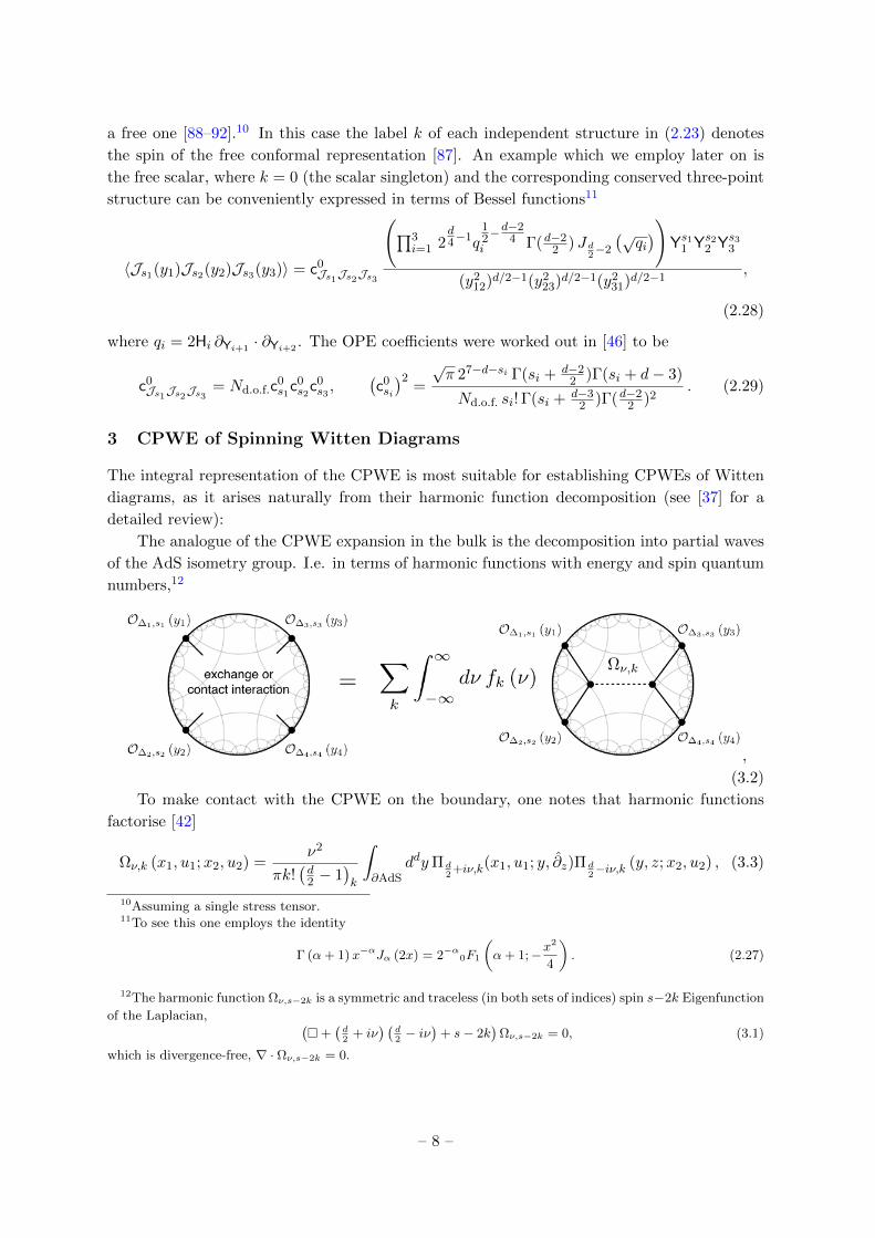
The integral representation of the CPWE is most suitable for establishing CPWEs of Witten

diagrams, as it arises naturally from their harmonic function decomposition (see [37] for a

detailed review):

The analogue of the CPWE expansion in the bulk is the decomposition into partial waves

of the AdS isometry group. I.e. in terms of harmonic functions with energy and spin quantum

numbers,12

,

(3.2)

To make contact with the CPWE on the boundary, one notes that harmonic functions

factorise [42]

Ων,k (x1, u1;x2, u2) =ν2

πk!(d2 − 1

)k

∫∂AdS

ddyΠ d2

+iν,k(x1, u1; y, ∂z)Π d2−iν,k (y, z;x2, u2) , (3.3)

10Assuming a single stress tensor.11To see this one employs the identity

Γ (α+ 1)x−αJα (2x) = 2−α0F1

(α+ 1;−x

2

4

). (2.27)

12The harmonic function Ων,s−2k is a symmetric and traceless (in both sets of indices) spin s−2k Eigenfunction

of the Laplacian, ( +

(d2

+ iν) (

d2− iν

)+ s− 2k

)Ων,s−2k = 0, (3.1)

which is divergence-free, ∇ · Ων,s−2k = 0.

– 8 –

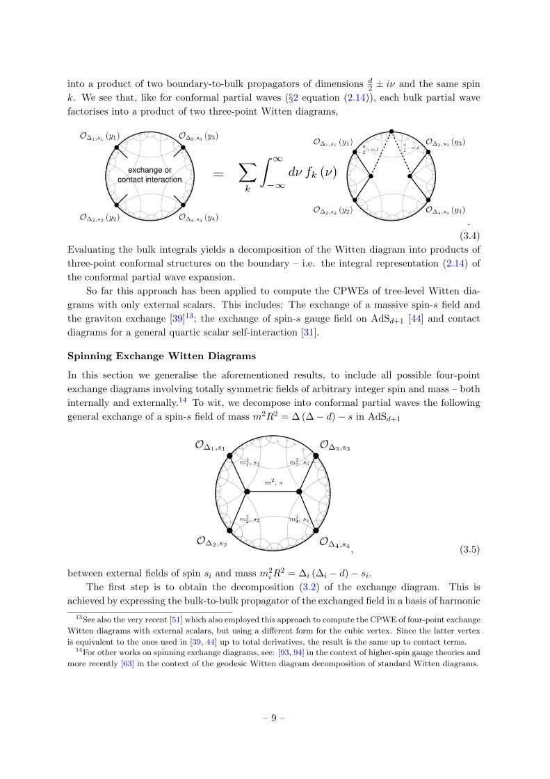
into a product of two boundary-to-bulk propagators of dimensions d2 ± iν and the same spin

k. We see that, like for conformal partial waves (§2 equation (2.14)), each bulk partial wave

factorises into a product of two three-point Witten diagrams,

.

(3.4)

Evaluating the bulk integrals yields a decomposition of the Witten diagram into products of

three-point conformal structures on the boundary – i.e. the integral representation (2.14) of

the conformal partial wave expansion.

So far this approach has been applied to compute the CPWEs of tree-level Witten dia-

grams with only external scalars. This includes: The exchange of a massive spin-s field and

the graviton exchange [39]13; the exchange of spin-s gauge field on AdSd+1 [44] and contact

diagrams for a general quartic scalar self-interaction [31].

Spinning Exchange Witten Diagrams

In this section we generalise the aforementioned results, to include all possible four-point

exchange diagrams involving totally symmetric fields of arbitrary integer spin and mass – both

internally and externally.14 To wit, we decompose into conformal partial waves the following

general exchange of a spin-s field of mass m2R2 = ∆ (∆− d)− s in AdSd+1

, (3.5)

between external fields of spin si and mass m2iR

2 = ∆i (∆i − d)− si.The first step is to obtain the decomposition (3.2) of the exchange diagram. This is

achieved by expressing the bulk-to-bulk propagator of the exchanged field in a basis of harmonic

13See also the very recent [51] which also employed this approach to compute the CPWE of four-point exchange

Witten diagrams with external scalars, but using a different form for the cubic vertex. Since the latter vertex

is equivalent to the ones used in [39, 44] up to total derivatives, the result is the same up to contact terms.14For other works on spinning exchange diagrams, see: [93, 94] in the context of higher-spin gauge theories and

more recently [63] in the context of the geodesic Witten diagram decomposition of standard Witten diagrams.

– 9 –

functions [39, 44, 95], which we review for massive fields in §3.2.1 and for massless fields in

§3.2.2. This leads to the decomposition (3.4) of the exchange diagram (3.5) into products

of tree-level three-point Witten diagrams, whose evaluation leads to the sought-for conformal

partial wave expansion via identification with the integral form (2.20) of the conformal partial

waves.

3.1 Spinning three-point Witten diagrams

In the light of the decomposition (3.2) of Witten diagrams, a key step to obtain CPWEs

of spinning diagrams is therefore the evaluation of tree-level three-point Witten diagrams

involving fields of arbitrary integer spin and mass. For parity even theories, this was carried

out in [46] in general dimensions, whose results we review here and also further supplement

with new ones.

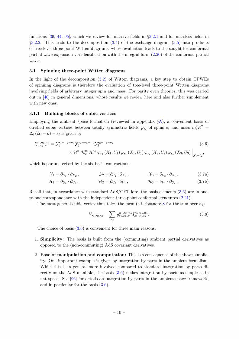
3.1.1 Building blocks of cubic vertices

Employing the ambient space formalism (reviewed in appendix §A), a convenient basis of

on-shell cubic vertices between totally symmetric fields ϕsi of spins si and mass m2iR

2 =

∆i (∆i − d)− si is given by

In1,n2,n3s1,s2,s3 = Ys1−n2−n3

1 Ys2−n3−n12 Ys3−n1−n2

3 (3.6)

×Hn11 H

n22 H

n33 ϕs1 (X1, U1)ϕs1 (X1, U1)ϕs2 (X2, U2)ϕss (X3, U3)

∣∣∣Xi=X

,

which is parameterised by the six basic contractions

Y1 = ∂U1 · ∂X2 , Y2 = ∂U2 · ∂X3 , Y3 = ∂U3 · ∂X1 , (3.7a)

H1 = ∂U2 · ∂U3 , H2 = ∂U3 · ∂U1 , H3 = ∂U1 · ∂U2 . (3.7b)

Recall that, in accordance with standard AdS/CFT lore, the basis elements (3.6) are in one-

to-one correspondence with the independent three-point conformal structures (2.21).

The most general cubic vertex thus takes the form (c.f. footnote 8 for the sum over ni)

Vs1,s2,s3 =∑ni

gn1,n2,n3s1,s2,s3 I

n1,n2,n3s1,s2,s3 . (3.8)

The choice of basis (3.6) is convenient for three main reasons:

1. Simplicity: The basis is built from the (commuting) ambient partial derivatives as

opposed to the (non-commuting) AdS covariant derivatives.

2. Ease of manipulation and computation: This is a consequence of the above simplic-

ity. One important example is given by integration by parts in the ambient formalism.

While this is in general more involved compared to standard integration by parts di-

rectly on the AdS manifold, the basis (3.6) makes integration by parts as simple as in

flat space. See [96] for details on integration by parts in the ambient space framework,

and in particular for the basis (3.6).

– 10 –

3. Physical interpretation: Any vertex expressed in terms of covariant derivatives can

straightforwardly be cast in terms of the basis (3.6), and vice versa, using (see §A)

∇A = PBA∂

∂XB− XB

X2ΣAB, (3.9)

where

ΣAB = U[A∂

∂UB ]= UA

∂

∂UB− UB

∂

∂UA, (3.10)

is the spin connection in the ambient generating function formalism. See appendix B of

[46] for more details about radial reduction.

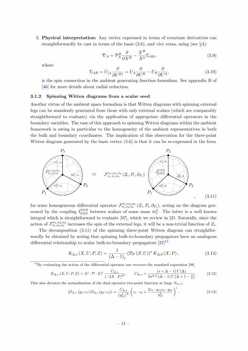
3.1.2 Spinning Witten diagrams from a scalar seed

Another virtue of the ambient space formalism is that Witten diagrams with spinning external

legs can be seamlessly generated from those with only external scalars (which are comparably

straightforward to evaluate) via the application of appropriate differential operators in the

boundary variables. The ease of this approach to spinning Witten diagrams within the ambient

framework is owing in particular to the homogeneity of the ambient representatives in both

the bulk and boundary coordinates. The implication of this observation for the three-point

Witten diagram generated by the basis vertex (3.6) is that it can be re-expressed in the form

, (3.11)

for some homogeneous differential operator Fn1,n2,n3s1,s2,s3 (Zi, Pi, ∂Pi), acting on the diagram gen-

erated by the coupling I0,0,00,0,0 between scalars of some mass m2

i . The latter is a well known

integral which is straightforward to evaluate [97], which we review in §D. Naturally, since the

action of Fn1,n2,n3s1,s2,s3 increases the spin of the external legs, it will be a non-trivial function of Zi.

The decomposition (3.11) of the spinning three-point Witten diagram can straightfor-

wardly be obtained by noting that spinning bulk-to-boundary propagators have an analogous

differential relationship to scalar bulk-to-boundary propagators [37]15

K∆,s (X,U ;P,Z) =1

(∆− 1)s(DP (Z;U))sK∆,0 (X;P ) , (3.14)

15By evaluating the action of the differential operator one recovers the standard expression [98]

K∆,s (X,U ;P,Z) = (U · P · Z)sC∆,s

(−2X · P )∆, C∆,s =

(s+ ∆− 1) Γ (∆)

2πd/2 (∆− 1) Γ(∆ + 1− d

2

) . (3.12)

This also dictates the normalisation of the dual operator two-point function at large Nd.o.f

〈O∆,s (y1; z1)O∆,s (y2; z2)〉 =C∆,s

(y212)∆

(z1 · z2 +

2z1 · y12z2 · y21

y212

)s. (3.13)

– 11 –

with differential operator

DP (Z;U) = (Z · U)

(Z · ∂

∂Z− P · ∂

∂P

)+ (P · U)

(Z · ∂

∂P

). (3.15)

Ambient partial derivatives of spinning bulk-to-boundary propagators, which arise natu-

rally from the basis (3.6), can readily be expressed in a similar form:

(Uj · ∂X)nK∆,s (X,Ui;P,Z) =1

(∆− 1)s(DP (Z;U))s (Ui · ∂X)nK∆,0 (X;P ) (3.16)

with

(Ui · ∂X)nK∆,0 (X;P ) = 2n (∆)n (Ui · P )nK∆+n,0 (X;P ) . (3.17)

This further illustrates the convenience of the choice of basis (3.6).

Employing the expression for spinning bulk-to-boundary propagators (3.16) one then ob-

tains

Fn1,n2,n3s1,s2,s3 =

2s1+s2+s3 (∆1)s3 (∆2)s1 (∆3)s2(∆1 − 1)s1 (∆2 − 1)s2 (∆3 − 1)s3 (s1)! (s2)! (s3)!

(3.18)

×Hn11 H

n22 H

n33 H

s21 H

s32 H

s13 D

s1P1Ds2P2Ds3P3

(U1 · P1

)s3 (U2 · P2

)s2 (U3 · P3

)s1where for concision we defined si = si − ni−1 − ni+1 and introduced the auxiliary vector Uiwhich enters the contraction Hi = ∂Ui−1 · ∂Ui+1

. The mass of each scalar entering the seed

vertex on the RHS of (3.11) is given in terms of the quantum numbers of the original spinning

fields on the LHS:

m2iR

2 = ∆i(∆i − d) with ∆i = ∆i + si+2 − ni − ni+1. (3.19)

What remains to obtain the result for the spinning Witten diagram in the LHS of (3.11)

is to simply insert the result (D.5) for the scalar seed on the RHS and then act with the

differential operator (3.18). Denoting the amplitude by An1,n2,n3s1,s2,s3;τ1,τ2,τ3 , this procedure yields16

An1,n2,n3s1,s2,s3;τ1,τ2,τ3 (y1, y2, y3) = P3

∑α,β,δ,ω,γ

3∏i=1

(−1)si−ni−δi+αi+βi2si−ni−γi−δi−ωini!(αi + βi)!(si − ni+1 − ni−1)!

γi!δi!αi!ωi!(βi + δi+1 − ni+1 + 1)!

×(αi + βi + ∆i)si+δi(i+1)−γi+1−ni+1−ωi+1−∆i

(αi + βi − γi+1 − γi−1 − ωi+1 + 1)!(si − αi − ni+1 − ni−1 − ωi−1 + 1)!(ni+1 + ni−1 − βi − δi+1 − δi−1 + 1)!

× Hγ1+δ1+ω11 Hγ2+δ2+ω2

2 Hγ3+δ3+ω33 Ys1−γ2−γ3−δ2−δ3−ω2−ω3

1 Ys2−γ1−γ3−δ1−δ3−ω1−ω32 Ys3−γ1−γ2−δ1−δ2−ω1−ω2

3 ,

where i ∼= i+ 3.

16The summation symbol is defined as:

∑α,β,δ,ω,γ

≡sκ−kκ∑ακ=0

kκ∑βκ=0

nκ∑δκ=0

ακ−1+βκ−1∑ωκ=0

ακ−1+βκ−1∑γκ=0

, (3.20)

– 12 –

The pre-factor is given by

P3 =1

16πd1

(y12)δ12(y23)δ23(y31)δ31Γ

(∑α

( τα2 + sα − nα)− d2

)3∏i=1

Γ(∆i − 1)(∆i + si − 1)

Γ(∆i + 1− d

2

) ,

where

δ(i−1)(i+1) =1

2(τi−1 + τi+1 − τi) , τi = ∆i − si . (3.21)

While the basis (3.6) is convenient as a means to evaluate spinning Witten diagrams,

the resulting one-to-one map (3.21) between the bulk basis elements (3.6) and the canonical

basis (2.21) of three-point conformal structures is rather involved. In the following section we

introduce an alternative bulk and boundary pair of bases, through which the aforementioned

bulk-to-boundary mapping simplifies dramatically and moreover allows to elegantly re-sum the

expression (3.21).

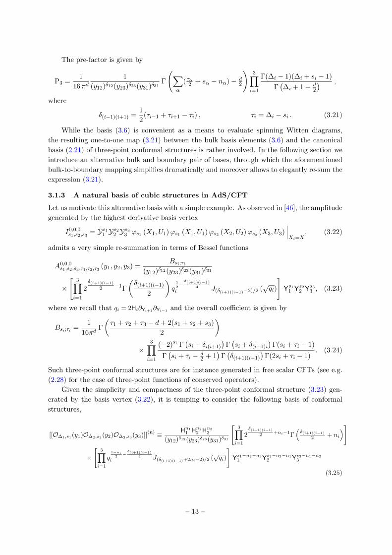
3.1.3 A natural basis of cubic structures in AdS/CFT

Let us motivate this alternative basis with a simple example. As observed in [46], the amplitude

generated by the highest derivative basis vertex

I0,0,0s1,s2,s3 = Ys11 Y

s22 Y

s33 ϕs1 (X1, U1)ϕs1 (X1, U1)ϕs2 (X2, U2)ϕss (X3, U3)

∣∣∣Xi=X

, (3.22)

admits a very simple re-summation in terms of Bessel functions

A0,0,0s1,s2,s3;τ1,τ2,τ3 (y1, y2, y3) =

Bsi;τi(y12)δ12(y23)δ23(y31)δ31

×

[3∏i=1

2δ(i+1)(i−1)

2 −1Γ

(δ(i+1)(i−1)

2

)q

12−δ(i+1)(i−1)

4i J(δ(i+1)(i−1)−2)/2 (

√qi)

]Ys11 Ys22 Ys33 , (3.23)

where we recall that qi = 2Hi∂Yi+1∂Yi−1 and the overall coefficient is given by

Bsi;τi =1

16πdΓ

(τ1 + τ2 + τ3 − d+ 2(s1 + s2 + s3)

2

)×

3∏i=1

(−2)si Γ(si + δi(i+1)

)Γ(si + δ(i−1)i

)Γ(si + τi − 1)

Γ(si + τi − d

2 + 1)

Γ(δ(i+1)(i−1)

)Γ(2si + τi − 1)

. (3.24)

Such three-point conformal structures are for instance generated in free scalar CFTs (see e.g.

(2.28) for the case of three-point functions of conserved operators).

Given the simplicity and compactness of the three-point conformal structure (3.23) gen-

erated by the basis vertex (3.22), it is temping to consider the following basis of conformal

structures,

[[O∆1,s1(y1)O∆2,s2(y2)O∆3,s3(y3)]](n) ≡ Hn1

1 Hn22 Hn3

3

(y12)δ12(y23)δ23(y31)δ31

[3∏i=1

2δ(i+1)(i−1)

2 +ni−1Γ(δ(i+1)(i−1)

2 + ni

)]

×

[3∏i=1

q1−ni

2 −δ(i+1)(i−1)

4i J(δ(i+1)(i−1)+2ni−2)/2 (

√qi)

]Ys1−n2−n3

1 Ys2−n3−n12 Ys3−n1−n2

3

(3.25)

– 13 –

in the view of simplifying the map between bulk and boundary structures.

Indeed, working iteratively one finds that the conformal structure (3.25) is generated by

the bulk vertex17

In1,n2,n3s1,s2,s3 =

∑mi

Cn1,n2,n3s1,s2,s3;m1,m2,m3

Im1,m2,m3s1,s2,s3 , (3.26)

with coefficients Cn1,n2,n3s1,s2,s3;m1,m2,m3 given by

Cn1,n2,n3s1,s2,s3;m1,m2,m3

=(d−2(s1+s2+s3−1)−(τ1+τ2+τ3)

2

)m1+m2+m3

×3∏i=1

[2mi

(nimi

)(ni + δ(i+1)(i−1) − 1)mi

], (3.27)

In particular, denoting the three-point amplitude generated by each basis element (3.26) by

An1,n2,n3s1,s2,s3;τ1,τ2,τ3 , we have:18

An1,n2,n3s1,s2,s3;τ1,τ2,τ3 (y1, y2, y3) = B(si;ni; τi) [[O∆1,s1(y1)O∆2,s2(y2)O∆3,s3(y3)]](n) , (3.28)

with the coefficient B(si;ni; τi) given by

B(si;ni; τi) = π−d(−2)(s1+s2+s3)−(n1+n2+n3)−4 Γ(τ1+τ2+τ3−d+2(s1+s2+s3)

2

)×

3∏i=1

Γ(si − ni+1 + ni−1 + τi+τi+1−τi−1

2

)Γ(si + ni+1 − ni−1 + τi+τi−1−τi+1

2

)Γ(si + ni+1 + ni−1 + τi − 1)

Γ(si + τi − d

2 + 1)

Γ(

2ni + τi+1+τi−1−τi2

)Γ(2si + τi − 1)

.

(3.29)

Given a CFTd, the result (3.28) provides the complete holographic reconstruction of all

cubic couplings involving totally symmetric fields in the putative dual theory on AdSd+1.19

Relation between bulk basis

To conclude it is useful to spell out the explicit dictionary between the building blocks (3.6),

which allow to straightforwardly evaluate spinning Witten diagrams, and the basis (3.26) in-

troduced in the previous section, which give a simple form for spinning three-point amplitudes.

Given a coupling of the form

Vs1,s2,s3 =∑ni

gn1,n2,n3s1,s2,s3 I

n1,n2,n3s1,s2,s3 , (3.30)

17For concision we define∑mi

=mins1,s2,n3∑

m3=0

mins1−n3,s3,n2∑n2=0

mins2−n3,s3−n2,n1∑n1=0

18Note, the vertices constructed here should not be confused with those written down in [51, 64] in the context

of geodesic Witten diagrams.19 Previous works on the holographic reconstruction of bulk interactions from CFT correlation functions

include: [31, 37, 43–46] for cubic and quartic couplings in the context of higher-spin holography. More recently

cubic couplings have been extracted for the bulk dual of the SYK model in [47].

– 14 –

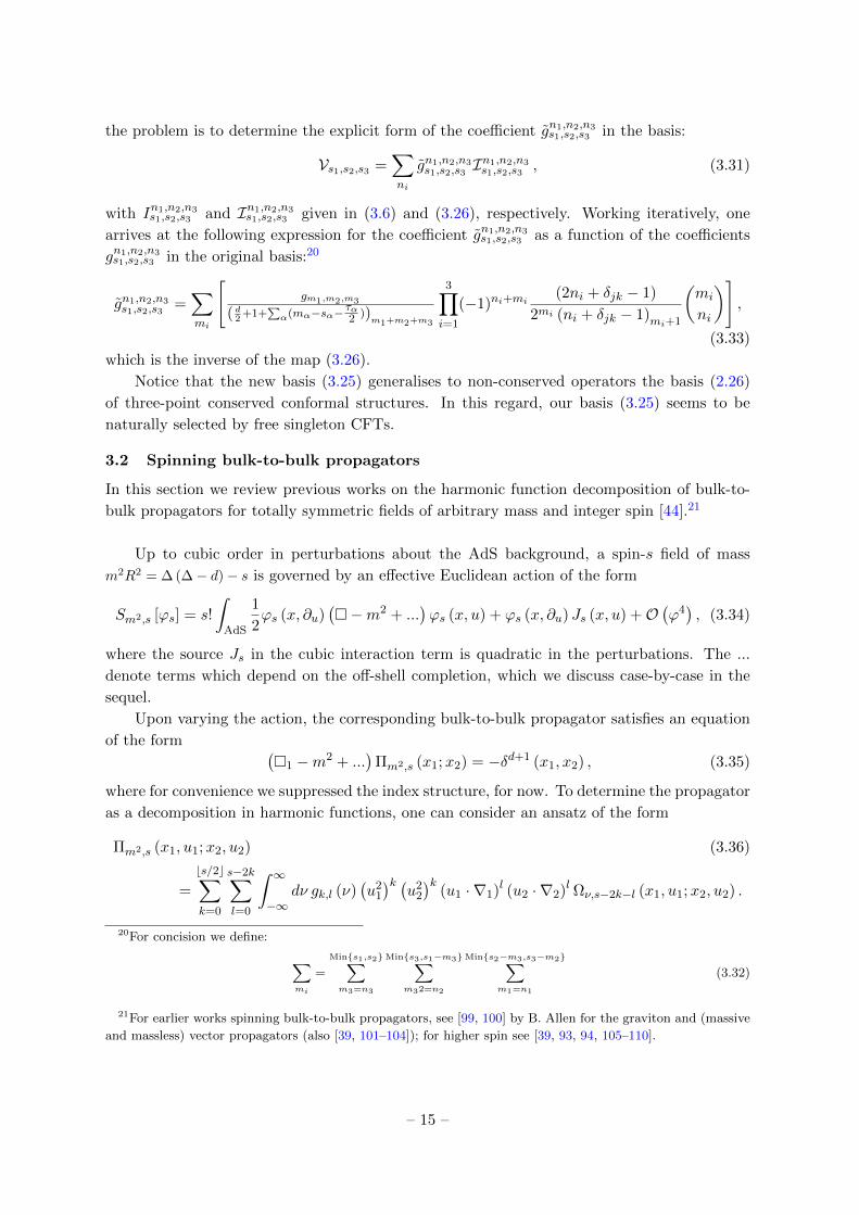
the problem is to determine the explicit form of the coefficient gn1,n2,n3s1,s2,s3 in the basis:

Vs1,s2,s3 =∑ni

gn1,n2,n3s1,s2,s3 I

n1,n2,n3s1,s2,s3 , (3.31)

with In1,n2,n3s1,s2,s3 and In1,n2,n3

s1,s2,s3 given in (3.6) and (3.26), respectively. Working iteratively, one

arrives at the following expression for the coefficient gn1,n2,n3s1,s2,s3 as a function of the coefficients

gn1,n2,n3s1,s2,s3 in the original basis:20

gn1,n2,n3s1,s2,s3 =

∑mi

[gm1,m2,m3

( d2 +1+∑α(mα−sα− τα2 ))

m1+m2+m3

3∏i=1

(−1)ni+mi(2ni + δjk − 1)

2mi (ni + δjk − 1)mi+1

(mi

ni

)],

(3.33)

which is the inverse of the map (3.26).

Notice that the new basis (3.25) generalises to non-conserved operators the basis (2.26)

of three-point conserved conformal structures. In this regard, our basis (3.25) seems to be

naturally selected by free singleton CFTs.

3.2 Spinning bulk-to-bulk propagators

In this section we review previous works on the harmonic function decomposition of bulk-to-

bulk propagators for totally symmetric fields of arbitrary mass and integer spin [44].21

Up to cubic order in perturbations about the AdS background, a spin-s field of mass

m2R2 = ∆ (∆− d)− s is governed by an effective Euclidean action of the form

Sm2,s [ϕs] = s!

∫AdS

1

2ϕs (x, ∂u)

(−m2 + ...

)ϕs (x, u) + ϕs (x, ∂u) Js (x, u) +O

(ϕ4), (3.34)

where the source Js in the cubic interaction term is quadratic in the perturbations. The ...

denote terms which depend on the off-shell completion, which we discuss case-by-case in the

sequel.

Upon varying the action, the corresponding bulk-to-bulk propagator satisfies an equation

of the form (1 −m2 + ...

)Πm2,s (x1;x2) = −δd+1 (x1, x2) , (3.35)

where for convenience we suppressed the index structure, for now. To determine the propagator

as a decomposition in harmonic functions, one can consider an ansatz of the form

Πm2,s (x1, u1;x2, u2) (3.36)

=

bs/2c∑k=0

s−2k∑l=0

∫ ∞−∞

dν gk,l (ν)(u2

1

)k (u2

2

)k(u1 · ∇1)l (u2 · ∇2)l Ων,s−2k−l (x1, u1;x2, u2) .

20For concision we define: ∑mi

=

Mins1,s2∑m3=n3

Mins3,s1−m3∑m32=n2

Mins2−m3,s3−m2∑m1=n1

(3.32)

21For earlier works spinning bulk-to-bulk propagators, see [99, 100] by B. Allen for the graviton and (massive

and massless) vector propagators (also [39, 101–104]); for higher spin see [39, 93, 94, 105–110].

– 15 –

The functions gk,l (ν) are fixed by requiring that the equation of motion (3.35) is satisfied.

We first review the solution for massive spinning fields before moving on to the massless

case, where one has the additional requirement of gauge invariance.

3.2.1 Massive case

The Lagrangian formulation for freely propagating totally symmetric massive fields of arbitrary

spin was first considered by Singh and Hagen in the 70’s [111, 112].22 In order for the Fierz-

Pauli physical state conditions [117–119](−m2

)ϕs (x, u) = 0, (∂u · ∇)ϕs (x, u) = 0, (∂u · ∂u)ϕs (x, u) = 0, (3.37)

to be recovered upon varying the action, the field content consists of the traceless field ϕs, and

additional traceless auxiliary fields of ranks s− 2, s− 3, ..., 0 which vanish on-shell.23

The complete off-shell form of the free Lagrangian is involved, and is moreover currently

unavailable in its entirety on an AdS background. On the other hand, the terms which have

not yet been identified explicitly are those which vanish on-shell (i.e. the ... in (3.34)) and thus

only generate contact terms in exchange amplitudes. The latter are not universal contributions,

as they are highly dependent on the field frame. For our purposes it is therefore not necessary

to keep track of such terms,24 and we can solve the following equation for the massive spin-s

bulk-to-bulk propagator(1 −m2

)Πm2,s (x1, u1;x2, u2) = −(u1 · u2)s δd+1 (x1, x2) , (3.38)

where the notation • signifies a traceless projection.

Since in this case the field is traceless, the following ansatz can be considered for the

bulk-to-bulk propagator

Πm2,s (x1, w1;x2, w2) =

s∑l=0

∫ ∞−∞

dν gl (ν) (w1 · ∇1)l (w2 · ∇2)l Ων,s−l (x1, w1;x2, w2) , (3.39)

where the null auxiliary vectors w2i = 0 enforce tracelessness. Substituting into the equation

of motion (3.38), one finds [44]

gl (ν) =1(

d2 −∆

)2+ ν2 − l + l(d+ 2s− `− 1)

(3.40)

×2l (s− l + 1)l

(d2 + s− l − 1

2

)l

l! (d+ 2s− 2l − 1)l(d2 + s− l + iν

)l

(d2 + s− l − iν

)l

.

Before moving on to consider the massless case, let us briefly highlight some generic features

of the propagator (3.39):

22See also [113–116].23See [120, 121] for an alternative formulation of the free massive Lagrangian in terms of curvatures, free from

such auxiliary fields. Their removal, however, comes at the price of introducing non-localities.24When it is feasible we do keep track of contact terms, such as for the massless case introduced in the

following section.

– 16 –

• The traceless and transverse part of the propagator (corresponding to l = 0 in (3.39))

ΠTTm2,s (x1;x2) =

∫ ∞−∞

dν(d2 −∆

)2+ ν2

Ων,s (x1;x2) , (3.41)

is universal, and encodes the propagating degrees of freedom.

• The remaining contributions from harmonic functions of spin < s (the l > 0 in (3.39))

are purely off-shell, and generate only contact terms in exchange amplitudes.

3.2.2 Massless case

On contrast to the massive case discussed in the previous section, the construction of free La-

grangians for massless fields is somewhat simplified owing to the additional guidance provided

by gauge invariance.

Recalling that the concept of masslessness in AdS is slightly deformed owing to the back-

ground curvature, requiring gauge invariance of the Fierz-Pauli system (3.37) under the gauge

transformation

δξϕs (x, u) = (u · ∇) ξs−1 (x, u) , (3.42)

fixes ∆ = s+ d− 2 in the mass m2R2 = ∆ (∆− d)− s. The complete off-shell Lagrangian form

was determined by Fronsdal in the 70’s [122], and reads

S(2)Fronsdal [ϕs] =

s!

2

∫AdSd+1

ϕs (x; ∂u)Gs (x;u) , (3.43)

where Gs is the corresponding spin-s generalisation of the linearised Einstein tensor

Gs (x;u) =

(1− 1

4u2 ∂u · ∂u

)Fs (x;u,∇, ∂u)ϕs (x, u) , (3.44)

with Fs the so-called Fronsdal operator

Fs(x, u,∇, ∂u) = −m2 − u2(∂u · ∂u)− (u · ∇)

((∇ · ∂u)− 1

2(u · ∇)(∂u · ∂u)

). (3.45)

The latter is fixed by invariance under linearised spin-s gauge transformations (3.42) with

symmetric and traceless rank s− 1 gauge parameter ξs−1.25 The Bianchi identity

(∂u · ∇)Gs (x, u) = 0 (3.46)

requires that the field ϕs is double-traceless26

(∂u · ∂u)2 ϕs (x, u) = 0. (3.47)

25Alternative formulations have been developed which eliminate this algebraic trace constraint on the gauge

parameter, however they come at the price of introducing introducing non-localities [123] or auxiliary fields

[93, 124, 125].26Note that the double-trace of ϕs is gauge invariant owing to the tracelessness of the gauge parameter.

Forgoing the double-traceless constraint (3.47) without introducing auxiliary fields (apart from deforming the

Bianchi identity (3.46) and thus requiring a modification of the action (3.43)) would lead to the propagation

of non-unitary modes, which one may try to kill by imposing appropriate boundary conditions. This has been

shown to be possible in flat space [125] though it is not yet clear if this approach can be extended to AdS

space-times, or if it is compatible with introducing a source. For this reason we stick to the standard Fronsdal

formulation (3.43) with double-trace constraint (3.47).

– 17 –

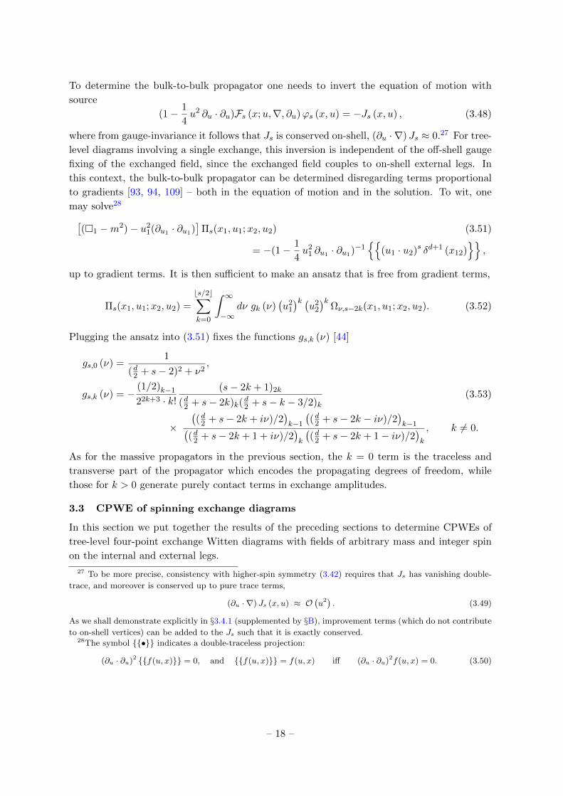
To determine the bulk-to-bulk propagator one needs to invert the equation of motion with

source

(1− 1

4u2 ∂u · ∂u)Fs (x;u,∇, ∂u)ϕs (x, u) = −Js (x, u) , (3.48)

where from gauge-invariance it follows that Js is conserved on-shell, (∂u · ∇) Js ≈ 0.27 For tree-

level diagrams involving a single exchange, this inversion is independent of the off-shell gauge

fixing of the exchanged field, since the exchanged field couples to on-shell external legs. In

this context, the bulk-to-bulk propagator can be determined disregarding terms proportional

to gradients [93, 94, 109] – both in the equation of motion and in the solution. To wit, one

may solve28[(1 −m2)− u2

1(∂u1 · ∂u1)]

Πs(x1, u1;x2, u2) (3.51)

= −(1− 1

4u2

1 ∂u1 · ∂u1)−1

(u1 · u2)s δd+1 (x12)

,

up to gradient terms. It is then sufficient to make an ansatz that is free from gradient terms,

Πs(x1, u1;x2, u2) =

bs/2c∑k=0

∫ ∞−∞

dν gk (ν)(u2

1

)k (u2

2

)kΩν,s−2k(x1, u1;x2, u2). (3.52)

Plugging the ansatz into (3.51) fixes the functions gs,k (ν) [44]

gs,0 (ν) =1

(d2 + s− 2)2 + ν2,

gs,k (ν) = −(1/2)k−1

22k+3 · k!

(s− 2k + 1)2k

(d2 + s− 2k)k(d2 + s− k − 3/2)k

(3.53)

×((d2 + s− 2k + iν)/2

)k−1

((d2 + s− 2k − iν)/2

)k−1(

(d2 + s− 2k + 1 + iν)/2)k

((d2 + s− 2k + 1− iν)/2

)k

, k 6= 0.

As for the massive propagators in the previous section, the k = 0 term is the traceless and

transverse part of the propagator which encodes the propagating degrees of freedom, while

those for k > 0 generate purely contact terms in exchange amplitudes.

3.3 CPWE of spinning exchange diagrams

In this section we put together the results of the preceding sections to determine CPWEs of

tree-level four-point exchange Witten diagrams with fields of arbitrary mass and integer spin

on the internal and external legs.

27 To be more precise, consistency with higher-spin symmetry (3.42) requires that Js has vanishing double-

trace, and moreover is conserved up to pure trace terms,

(∂u · ∇) Js (x, u) ≈ O(u2) . (3.49)

As we shall demonstrate explicitly in §3.4.1 (supplemented by §B), improvement terms (which do not contribute

to on-shell vertices) can be added to the Js such that it is exactly conserved.28The symbol • indicates a double-traceless projection:

(∂u · ∂u)2 f(u, x) = 0, and f(u, x) = f(u, x) iff (∂u · ∂u)2f(u, x) = 0. (3.50)

– 18 –

3.3.1 Natural basis of conformal partial waves in AdS/CFT

To this end, it is useful to briefly discuss the integral form (2.20) of spinning conformal partial

waves in terms of the natural AdS/CFT basis (3.25) of three point conformal structures.

Employing this new basis, the spinning conformal partial waves of §2.2.2 read

Wn,m∆,s (yi) + shadow (3.54)


πd/2

∫ddy [[O∆1,s1(y1)O∆2,s2(y2)O∆,s(y)]](n) [[O∆,s(y)O∆3,s3(y3)O∆4,s4(y4)]](m),

where for convenience we repeat here the form of the basis elements (3.25)

[[O∆1,s1(y1)O∆2,s2(y2)O∆3,s3(y3)]](n) ≡ Hn1

1 Hn22 Hn3

3

(y12)δ12(y23)δ23(y31)δ31

[3∏i=1

2δ(i+1)(i−1)

2 +ni−1Γ(δ(i+1)(i−1)

2 + ni

)](3.55)

×

[3∏i=1

q1−ni

2 −δ(i+1)(i−1)

4i J(δ(i+1)(i−1)+2ni−2)/2 (

√qi)

]Ys1−n2−n3

1 Ys2−n3−n12 Ys3−n1−n2

3

In combination with the basis (3.26) of bulk cubic vertices, once the harmonic function

decomposition of a given spinning Witten diagram is known the choice of basis (3.54) of spin-

ning conformal partial waves makes its CPWE follow almost automatically. We demonstrate

this explicitly in the following section.

3.3.2 Generic spinning exchange diagram

We consider a generic tree-level four-point exchange of a spin-s field of mass m2 between fields

of spin si and mass m2i . This is depicted for the s-channel below,

. (3.56)

At this level the cubic vertices Vs,si,sj are kinematic, and are not constrained by any consistency

condition aside from the necessary requirement of respecting the AdS isometry. Expanded in

the natural basis (3.26), they read

Vs,si,sj =∑ni

gni,nj ,nsi,sj ,s I

ni,nj ,nsi,sj ,s , (3.57)

with arbitrary couplings gni,nj ,nsi,sj ,s .

– 19 –

The harmonic function decomposition decomposition follows upon insertion of the massive

spin-s bulk-to-bulk propagator (3.39)

.

(3.58)

What remains to determine the CPWE is to evaluate the three-point Witten diagrams on the

RHS, which can be carried out seamlessly by employing the tools developed in §3.1.

For this generic case we focus on the part of the exchange which encodes the propagating

degrees of freedom. These are carried by the traceless and transverse part of the bulk-to-bulk

propagator (3.41), and accordingly we focus on the l = 0 contribution in the harmonic function

decomposition (3.58). The latter is factorised into three-point Witten diagrams of the form:

, (3.59)

by virtue of the split representation (3.3) of the harmonic function. The amplitudes (3.59) can

be straightforwardly given in any basis of three-point conformal structures using the results of

§3.1. However, choosing to expand the couplings (3.57) in the natural AdS/CFT basis (3.26)

of cubic vertices gives the following simple and compact form

As;τ± (yi, yj , y) =∑n

gnsAns;τ± (yi, yj , y) (3.60)

=∑n

gns B(s; n; τ±) [[O∆i,si(yi)O∆j ,sj (yj)O d2±iν,s(y)]](n)

where we defined the vectors s = (si, sj , s), n = (ni, nj , n) and τ± = (τi, τj ,d2 ± iν − s).

29

29In particular, gns = gni,nj ,nsi,sj ,s and An

s;τ is the amplitude (3.28) with labels s = (si, sj , s), n = (ni, nj , n) and

τ = (τi, τj ,d2± iν − s).

– 20 –

Using the integral representation of the conformal partial waves (3.54), one can then

immediately write down the CPWE of the s-channel exchange (3.56)30 31

Ass1,s2|s,m2|s3,s4 =

∫ ∞−∞

dν

ν2 +(d2 −∆

)2 ν2

πAs1,2;τ+

1,2(y1, y2, y)As3,4;τ−3,4

(y3, y4, y) + ...

=

∫ ∞−∞

dν∑n,m

cn,m (ν)Wn,md2

+iν,s(yi) + ... . (3.61)

with32

cn,m (ν) = −gns1,2gms3,4

B(s12; n; τ+1,2)B(s34; m; τ+

3,4)

ν2 +(d2 −∆

)2 2πd2−1Γ (iν + 1) ν(

iν + s+ d2 − 1

)Γ(iν + d

2 − 1) . (3.63)

This is the contour integral form (2.14) of the conformal partial wave expansion, reviewed in

§2.2.1. Recall that the functions cn,m (ν) encode the contribution from spin-s operators: A

pole at scaling dimension d2 + iν = λ in the lower-half ν-plane signifies a contribution from the

conformal multiplet [λ, s], whose residue gives the corresponding OPE coefficient. Separating

out such poles into a function pn,m (ν),

cn,m (ν) = cn,m (ν) pn,m (ν) , (3.64)

we have

pn,m (ν) =1

ν2 +(d2 −∆

)2 Γ

(2(s1+n−n2)+τ1+τ2+s−( d2 +iν)

2

)Γ

(2(s2+n−n1)+τ1+τ2+s−( d2 +iν)

2

)× Γ

(2(s3+m−m4)+τ3+τ4+s−( d2 +iν)

2

)Γ

(2(s4+m−m3)+τ3+τ4+s−( d2 +iν)

2

). (3.65)

There are two types of contributions, in accord with the standard lore on CPWEs of Witten

diagrams [28, 37, 75, 76, 102, 103, 126–133]:

1. Single-trace: This is the universal contribution to an exchange diagram, corresponding

to the exchange of the bulk single-particle state. Accordingly, it is generated by the pole-

factor in the traceless and transverse part of the bulk-to-bulk propagator (3.41), which

carries the propagating degrees of freedom. This translates into a pole at d2 + iν = ∆ in

(3.65), which coincides with the scaling dimension of the spin-s single-trace operator O∆,s

that is dual to the exchanged spin-s single-particle state of mass m2R2 = ∆ (∆− d)− s in

the bulk.

30Here, si,j = (si, sj , s), τ±i,j = (τi, τj ,

d2± iν − s), n = (n1, n2, n) and m = (m3,m4,m).

31The ... denote contact terms generated by the l > 0 contributions in the harmonic function decomposition

(3.58).32To obtain this expression we used that

B(s34;m; τ−3,4) =iκd−iν,sγ d

2+iν−s,sγ d

2+iν−s,s

2νπd/2C d2

+iν,s

B(s34;m; τ+3,4). (3.62)

– 21 –

2. Double-trace: The remaining contributions originate from contact terms, arising from

the collision of the two points that are integrated over the entire volume of AdS. This

generates 2-particle states in the bulk, which are dual to double-trace operators on the

conformal boundary. Accordingly, the corresponding poles are encoded in the factors

(3.29) arising from the integration over AdS. In the pole-function (3.65) these are the

origin of the two sets of Gamma function poles (p = 0, 1, 2, 3, ...)

1.

(d

2+ iν

)− s = τ1 + τ2 + 2 (s1 + n− n2 + p) ,

(d

2+ iν

)− s = τ1 + τ2 + 2 (s2 + n− n1 + p)

(3.66a)

2.

(d

2+ iν

)− s = τ3 + τ4 + 2 (s3 +m−m4 + p) ,

(d

2+ iν

)− s = τ3 + τ4 + 2 (s4 +m−m3 + p) ,

(3.66b)

corresponding to contributions from the two families [O∆1,s1O∆2,s2 ]s and [O∆3,s3O∆4,s4 ]sof spin-s double-trace operators, respectively. In the bulk, these correspond to 2-particle

states created, respectively, by ϕs1 with ϕs2 , and ϕs3 with ϕs4 .

Let us briefly comment on the l > 0 contributions to the harmonic function decomposition

(3.58). As explained earlier these are purely contact terms, and likewise generate double-

trace contributions [O∆1,s1O∆2,s2 ]s−l and [O∆3,s3O∆4,s4 ]s−l to the CPWE, but of lower

spin s− l.

3.4 Spinning exchanges in the type A higher-spin gauge theory

So far our dialogue has not been restricted to any particular theory of spinning fields. In recent

years, a lot of interest has been generated in theories of higher-spin gauge fields, owing in part

to the conjectured duality [134–139] between higher-spin gauge theories on AdS backgrounds

and free CFTs. In this section we apply the tools and results of the preceding sections to

compute all four-point exchange Witten diagrams in the simplest higher-spin gauge theory

for d > 2, which is known as the type A minimal higher-spin theory expanded about AdSd+1

[140].33 This theory is conjectured to be dual to the (singlet sector of the) free scalar O (N)

model in d-dimensions [137, 138].

The spectrum consists of a tower of totally symmetric even spin gauge fields (one for each

even spin s = 2, 4, 6, ...) and a parity even scalar of mass m20R

2 = −2(d− 2), which sits in the

higher-spin multiplet.

Before moving to the computation of the exchange amplitudes, we first review the result

for the metric-like cubic couplings established in [46].

3.4.1 Off-shell cubic couplings

The off-shell cubic couplings of the type A minimal higher-spin theory on AdSd+1 were deter-

mined in [46], for de Donder gauge.34 For tree-level exchanges we only require couplings with

33See [31, 37, 44, 46, 141–145] for other results on Witten diagrams in higher-spin gauge theories.34Note that although the result (3.67) for the complete cubic couplings was fixed using the holographic duality,

it was later verified [52] that the result solves the Noether procedure – i.e. requiring that each cubic coupling is

– 22 –

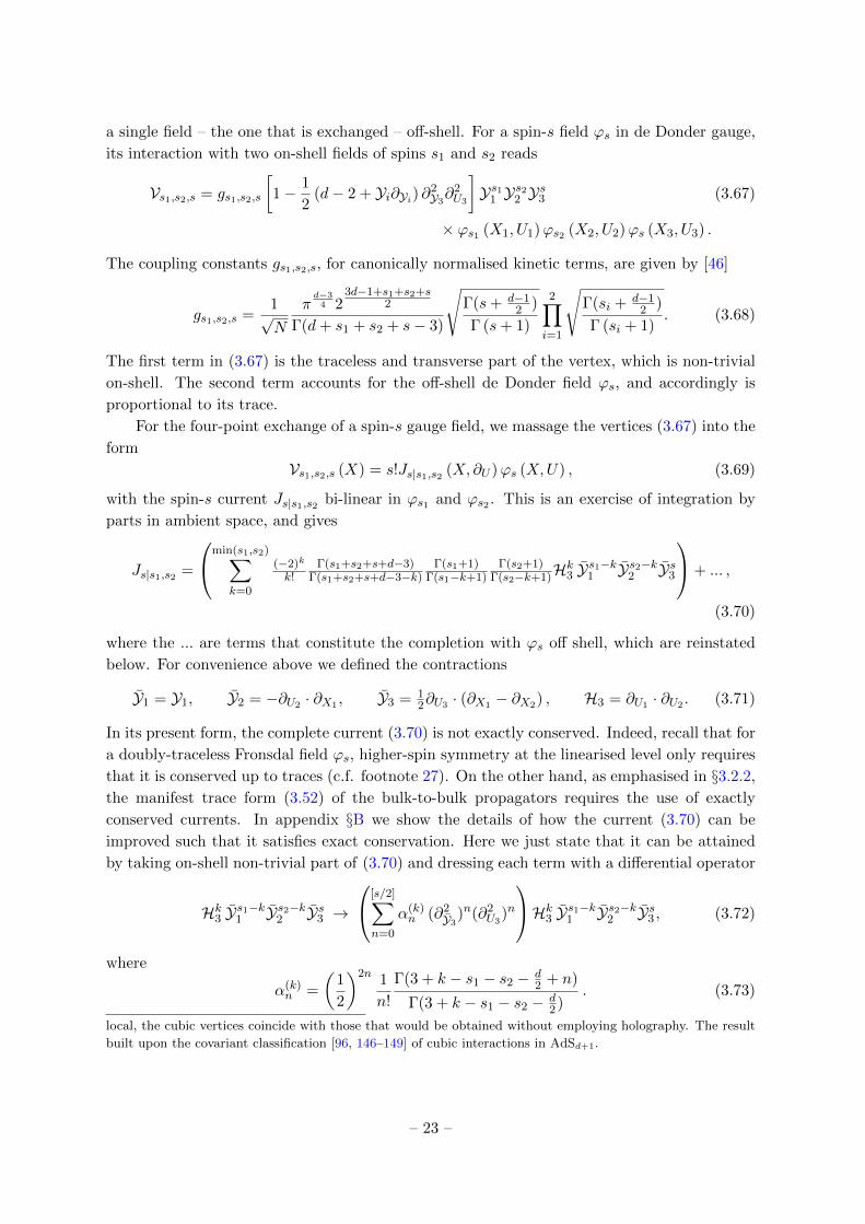
a single field – the one that is exchanged – off-shell. For a spin-s field ϕs in de Donder gauge,

its interaction with two on-shell fields of spins s1 and s2 reads

Vs1,s2,s = gs1,s2,s

[1− 1

2(d− 2 + Yi∂Yi) ∂2

Y3∂2U3

]Ys11 Y

s22 Y

s3 (3.67)

× ϕs1 (X1, U1)ϕs2 (X2, U2)ϕs (X3, U3) .

The coupling constants gs1,s2,s, for canonically normalised kinetic terms, are given by [46]

gs1,s2,s =1√N

πd−3

4 23d−1+s1+s2+s

2

Γ(d+ s1 + s2 + s− 3)

√Γ(s+ d−1

2 )

Γ (s+ 1)

2∏i=1

√Γ(si + d−1

2 )

Γ (si + 1). (3.68)

The first term in (3.67) is the traceless and transverse part of the vertex, which is non-trivial

on-shell. The second term accounts for the off-shell de Donder field ϕs, and accordingly is

proportional to its trace.

For the four-point exchange of a spin-s gauge field, we massage the vertices (3.67) into the

form

Vs1,s2,s (X) = s!Js|s1,s2 (X, ∂U )ϕs (X,U) , (3.69)

with the spin-s current Js|s1,s2 bi-linear in ϕs1 and ϕs2 . This is an exercise of integration by

parts in ambient space, and gives

Js|s1,s2 =

min(s1,s2)∑k=0

(−2)k

k!Γ(s1+s2+s+d−3)

Γ(s1+s2+s+d−3−k)Γ(s1+1)

Γ(s1−k+1)Γ(s2+1)

Γ(s2−k+1)Hk3 Y

s1−k1 Ys2−k2 Ys3

+ ... ,

(3.70)

where the ... are terms that constitute the completion with ϕs off shell, which are reinstated

below. For convenience above we defined the contractions

Y1 = Y1, Y2 = −∂U2 · ∂X1 , Y3 = 12∂U3 · (∂X1 − ∂X2) , H3 = ∂U1 · ∂U2 . (3.71)

In its present form, the complete current (3.70) is not exactly conserved. Indeed, recall that for

a doubly-traceless Fronsdal field ϕs, higher-spin symmetry at the linearised level only requires

that it is conserved up to traces (c.f. footnote 27). On the other hand, as emphasised in §3.2.2,

the manifest trace form (3.52) of the bulk-to-bulk propagators requires the use of exactly

conserved currents. In appendix §B we show the details of how the current (3.70) can be

improved such that it satisfies exact conservation. Here we just state that it can be attained

by taking on-shell non-trivial part of (3.70) and dressing each term with a differential operator

Hk3 Ys1−k1 Ys2−k2 Ys3 →

[s/2]∑n=0

α(k)n (∂2

Y3)n(∂2

U3)n

Hk3 Ys1−k1 Ys2−k2 Ys3 , (3.72)

where

α(k)n =

(1

2

)2n 1

n!

Γ(3 + k − s1 − s2 − d2 + n)

Γ(3 + k − s1 − s2 − d2)

. (3.73)

local, the cubic vertices coincide with those that would be obtained without employing holography. The result

built upon the covariant classification [96, 146–149] of cubic interactions in AdSd+1.

– 23 –

3.4.2 Four-point exchange diagrams

Consider the four-point exchange of a spin-s gauge field between gauge fields of spin si in the

s-channel. The manifest trace form of the bulk-to-bulk propagator (3.52) gives the harmonic

function decomposition

, (3.74)

where the operator Jsi is the spin-si conserved current in the free scalar O (N) model dual to

the spin-si gauge field ϕsi in the bulk. The notation J (k) denotes the k-th trace of the conserved

current J , which arise from the trace structure of the bulk-to-bulk propagator contact terms.

The explicit form of J is given in §3.4.1, while its k-th trace is derived in §C.

To determine the CPWE, we therefore need to evaluate three-point Witten diagrams of

the form,

, (3.75)

which, employing the tools introduced in §3.1 entails expressing the cubic couplings in the

basis (3.26).

We focus first on the k = 0 contribution, which encodes the propagating degrees of freedom.

As we saw for the massive exchanges in §3.3.2, this is generated by the traceless and transverse

part of the bulk-to-bulk propagator (3.52). Accordingly, only the on-shell non-trivial (traceless

and transverse) part of the cubic couplings (3.67) contribute, whose explicit form we give here

for convenience:

VTTs1,s2,s (X) = gs1,s2,sYs11 Y

s22 Y

s3ϕs1 (X1, U1)ϕs2 (X2, U2)ϕs (X3, U3)

∣∣∣Xi=X

. (3.76)

Nicely, this is already in the natural AdS/CFT basis (3.26) and the amplitudes (3.75) for k = 0

can be immediately written down by employing the result (3.28)

As;τ± (yi, yj , y) = gsi,sj ,s B (s; 0; τ ) [[Jsi (yi)Jsj (yj)Od2±iν,s

(y)]]0, (3.77)

– 24 –

where here τ± =(d− 2, d− 2, d2 ± iν − s

)and n = (0, 0, 0).

Following the discussion of §3.3.2 for the generic case, one then obtains that the k = 0 term

in the harmonic function decomposition (3.74) of the exchange diagram yields the following

contributions to its CPWE

Ass1,s2|s|s3,s4 =

∫ ∞−∞

dν cs (ν)W 0,0d2

+iν,s(yi) + ... (3.78)

with

cs (ν) = −gs1,s2,sgs3,s4,sB(s12; 0; τ+)B(s34; 0; τ+)

ν2 +(s+ d

2 − 2)2 2π

d2−1Γ (iν + 1) ν(

iν + s+ d2 − 1

)Γ(iν + d

2 − 1) , (3.79)

where the pole function (3.65) in this case is given by

ps (ν) =1

ν2 +(s+ d

2 − 2)2 Γ

(2(s1+d−2)+s−( d2 +iν)

2

)Γ

(2(s2+d−2)+s−( d2 +iν)

2

)× Γ

(2(s3+d−2)+s−( d2 +iν)

2

)Γ

(2(s4+d−2)+s−( d2 +iν)

2

). (3.80)

In the following we discuss in detail the particular contributions.

Single-trace

In line with the discussion of the generic case in §3.3.2, the pole factor in the traceless and

transverse part of the bulk-to-bulk propagator (3.52) generates a pole in (3.80) at d2 + iν =

s + d − 2, which is the scaling dimension of the dual spin-s conserved current Js in the free

scalar O (N) model.

Furthermore, notice that for d2 +iν = s+d−2 the three-point conformal structure generated

by the k = 0 amplitude (3.77) coincides with the three-point conserved structure (2.28) in free

scalar theories. The corresponding spin-s conformal partial wave thus coincides with the con-

served conformal partial wave W0,0s1,s2|s|s3,s4 in the set (2.25), which represents the contribution

from the conserved operator Js to the four-point function 〈Js1Js2Js3Js4〉 in free scalar theories.

With the result (2.29) of all single-trace conserved current OPE coefficients in free scalar

theories, in this case we can confirm the standard expectation that the single-trace contribution

to an exchange Witten diagram coincides with the contribution from the same single-trace

operator in the CPWE of the dual CFT four-point function, when expanded in the same

channel. Indeed, using that [46, 52]35

gsi,sj ,sB(sij ; 0; d− 2, d− 2, d− 2)√Csi+d−2,siCsj+d−2,sjCs+d−2,s

= cJsiJsjJs , (3.81)

we have (closing the contour in the lower-half ν-plane)

− 2πiRes

[cs (ν)W 0,0

d2

+iν,s(yi) ,

d2 + iν = s+ d− 2

]= cJs1Js2JscJsJs3Js4W

0,0s1,s2|s|s3,s4 (yi) ,

(3.82)

as expected.

35Here we divide by the normalisation of the bulk-to-boundary propagators (3.12) to give unit normalisation

to the dual single-trace operator two point functions (3.13).

– 25 –

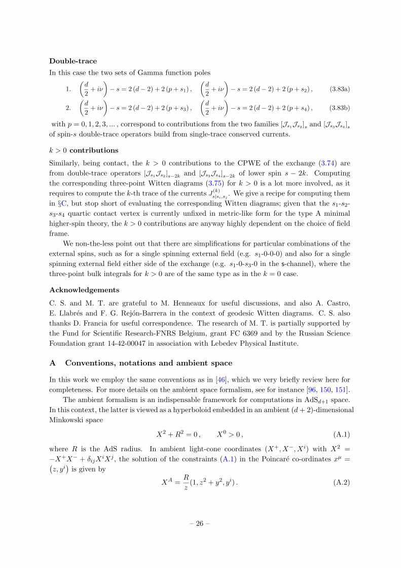
Double-trace

In this case the two sets of Gamma function poles

1.

(d

2+ iν

)− s = 2 (d− 2) + 2 (p+ s1) ,

(d

2+ iν

)− s = 2 (d− 2) + 2 (p+ s2) , (3.83a)

2.

(d

2+ iν

)− s = 2 (d− 2) + 2 (p+ s3) ,

(d

2+ iν

)− s = 2 (d− 2) + 2 (p+ s4) , (3.83b)

with p = 0, 1, 2, 3, ... , correspond to contributions from the two families [Js1Js2 ]s and [Js3Js4 ]sof spin-s double-trace operators build from single-trace conserved currents.

k > 0 contributions

Similarly, being contact, the k > 0 contributions to the CPWE of the exchange (3.74) are

from double-trace operators [Js1Js2 ]s−2k and [Js3Js4 ]s−2k of lower spin s − 2k. Computing

the corresponding three-point Witten diagrams (3.75) for k > 0 is a lot more involved, as it

requires to compute the k-th trace of the currents J (k)s|si,sj . We give a recipe for computing them

in §C, but stop short of evaluating the corresponding Witten diagrams; given that the s1-s2-

s3-s4 quartic contact vertex is currently unfixed in metric-like form for the type A minimal

higher-spin theory, the k > 0 contributions are anyway highly dependent on the choice of field

frame.

We non-the-less point out that there are simplifications for particular combinations of the

external spins, such as for a single spinning external field (e.g. s1-0-0-0) and also for a single

spinning external field either side of the exchange (e.g. s1-0-s3-0 in the s-channel), where the

three-point bulk integrals for k > 0 are of the same type as in the k = 0 case.

Acknowledgements

C. S. and M. T. are grateful to M. Henneaux for useful discussions, and also A. Castro,

E. Llabres and F. G. Rejon-Barrera in the context of geodesic Witten diagrams. C. S. also

thanks D. Francia for useful correspondence. The research of M. T. is partially supported by

the Fund for Scientific Research-FNRS Belgium, grant FC 6369 and by the Russian Science

Foundation grant 14-42-00047 in association with Lebedev Physical Institute.

A Conventions, notations and ambient space

In this work we employ the same conventions as in [46], which we very briefly review here for

completeness. For more details on the ambient space formalism, see for instance [96, 150, 151].

The ambient formalism is an indispensable framework for computations in AdSd+1 space.

In this context, the latter is viewed as a hyperboloid embedded in an ambient (d+ 2)-dimensional

Minkowski space

X2 +R2 = 0 , X0 > 0 , (A.1)

where R is the AdS radius. In ambient light-cone coordinates (X+, X−, Xi) with X2 =

−X+X− + δijXiXj , the solution of the constraints (A.1) in the Poincare co-ordinates xµ =(

z, yi)

is given by

XA =R

z(1, z2 + y2, yi) . (A.2)

– 26 –

Bulk fields

In order to obtain a one-to-one correspondence between fields on AdS and those living in

the higher-dimensional flat ambient space, one imposes constraints with defining the ambient

space extensions of the AdSd+1 fields [105]. Such restrictions are usually given as homogeneity

and tangentiality constraints. Employing a generating function formalism with intrinsic and

ambient auxiliary vectors uµ and UA, a symmetric rank-s tensor ϕs (x, u) intrinsic to the AdS

manifold is represented in ambient space by

ϕs (x, u) =1

s!ϕµ1...µs(x)uµ1 ...uµs → ϕs(X,U) =

1

s!ϕA1...As(X)UA1 . . . UAs . (A.3)

subject to the following homogeneity and tangentiality conditions

(X · ∂X −∆)ϕs(X,U) = 0 , (X · ∂U )ϕs(X,U) = 0 . (A.4)

Nicely, the conditions (A.4) imply that on-shell

∂2XϕA1...As = 0, (A.5)

for the ambient representative of the AdS field ϕs of mass m2R2 = ∆ (∆− d)− s.Let us stress that in imposing tangentiality and homogeneity conditions (A.4) one is im-

plicitly extending the AdS field to the full ambient space, where X2 plays the role of the radial

coordinate. This formalism is different from the manifestly intrinsic formalism (for instance

used in [39]) where one never moves away from the AdS manifold X2 = −R2.

The ambient representative of the AdS covariant derivative ∇µ takes the simple form

∇A = PBA∂

∂XB, (A.6)

and acts via

∇ = P ∂ P. (A.7)

Boundary fields

The boundary of AdSd+1 is identified with the null rays

P 2 = 0, P ∼ λP, λ 6= 0, (A.8)

where P gives the ambient space embedding of the CFT coordinate yi. It is convenient to

introduce the boundary analog of the auxiliary variables UA, which we refer to as ZA(y) and

extend to ambient space the null CFT auxiliary variable zi. Working in light cone coordinates

PA = (P+, P−, P i), with the gauge choice P+ = 1 one has

PA(y) = (1, y2, yi) and ZA(y) = (0, 2y · z, zi) . (A.9)

A symmetric rank-s boundary operator O∆,s of scaling dimension ∆ is represented by:36

O∆,s(y, z) =1

s!Oµ1...µs (y) zµ1 · · · zµs → O∆,s(P,Z) =

1

s!OA1...As (P )ZA1 · · ·ZAs ,

(A.10)

36Note that here z denotes the auxiliary vector zi and should not be confused with the radial Poincare

co-ordinate in (A.2).

– 27 –

where

(P · ∂P −∆)O∆,s(P,Z) = 0 , (P · ∂Z)O∆,s(P,Z) = 0 , (A.11)

and, being restricted to the null cone (A.8), there is an extra redundancy

OA1...As(P )→ OA1...As(P ) + P(A1ΛA2...As), (A.12)

PA1ΛA1...As−1 = 0, ΛA1...As−1(λP ) = λ−(∆+1)ΛA1...As−1(P ), ηA1A2ΛA1...As−1 = 0. (A.13)

B The improved current

In this appendix we detail the improvement of the higher-spin currents (3.70) to make them

exactly conserved. We begin with the traceless and transverse part of the current,

JTTs3|s1,s2 =

min(s1,s2)∑k=0

(−2)k

k!Γ(s1+s2+s3+d−3)

Γ(s1+s2+s3+d−3−k)Γ(s1+1)

Γ(s1−k+1)Γ(s2+1)

Γ(s2−k+1)Hk3 Y

s1−k1 Ys2−k2 Ys33 . (B.1)

On-shell, each monomial in the above is conserved. One can therefore study the structure of

the required improvements with ϕ3 off-shell for a given monomial

f (k)s1,s2,s3 = Hk3 Y

s1−k1 Ys2−k2 Ys33 . (B.2)

The combination of different monomials in (B.1) above is necessary to achieve on-shell gauge

invariance with respect to ϕ1 and ϕ2 which can be easily verified explicitly (see e.g. [96]).

In order to proceed to find the conserved improvement, the doubly-traceless condition on

ϕ3 together with the traceless condition on the corresponding gauge parameter needs to be

dropped. Not doing so would only recover a current whose traceless part is conserved. We

hence consider the following ansatz for the improvement, dressing each monomial (B.2) with

trace operators

F (k)s1,s2,s3 =

[s3/2]∑n=0

α(k)n (∂2

Y3)n(∂2

U3)n

f (k)s1,s2,s3 , (B.3)

where the derivative with respect to Y3 accounts for the fact that taking the trace lowers the

spin. The coefficients α(k)n in the ansatz (B.3) are fixed by requiring gauge invariance of the

vertex with ϕ3 off-shell and with traceless gauge parameter ξ3∫dX (U3 · ∇3 ξ3)F (k)

s1,s2,s3ϕ1ϕ2 = 0 . (B.4)

In the above the fields ϕ1 and ϕ2 are on-shell, while the integral sign (which in the following will

be omitted for ease of notation) implies that the above identity holds modulo total derivatives.

Employing the explicit form of the gradient operator:

U3 · ∇3 = U3 · ∂X3 −U3 ·X3

X23

(X3 · ∂X3 − U3 · ∂U3) , (B.5)

– 28 –

we arrive to the following conservation condition:

∞∑n=0

[2(n+ 1)α

(k)n+1 − 1

4 α(k)n [d+ 2(s1 + s2 − k − n)− 4]

](∂2Y3

)nf (k)s1,s2,s3(∂2

U3)n∂U3 · ∂X3 = 0 ,

(B.6)

which leads to the solution for α(k)n in the form

α(k)n =

(1

2

)2n 1

n!

Γ(3 + k − s1 − s2 − d2 + n)

Γ(3 + k − s1 − s2 − d2)

. (B.7)

C Trace of the currents

In order to evaluate the current exchange (3.74) with the manifest trace form of the propagator

(3.52), we are required to compute the n-th trace of the exactly conserved current derived in

the previous section. The process can be simplified by noting that in the present context the

traces are contracted with harmonic functions, where we encounter terms of the form

(∂2Y3

)nf (k)s1,s2,s3(∂2

U3)n(u2

3)q Ων,s3−2q

∣∣∣U3=0

, (C.1)

where u23 is the intrinsic symmetrised metric tensor written in generating function form, which

can be re-expressed in the ambient formalism as

u23 = U2

3 −U3 ·X3

X23

. (C.2)

To evaluate the trace one commutes the U3 contained in the(u2

3

)qto the far left hand

side, where the condition U3 = 0 can be applied. We first commute the u23 past the ∂2

U3, which,

employing the tracelessness of the harmonic functions, reads

(∂2U3

)n(u23)qΩν,s3−2q = Aqn(u2

3)q−nΩν,s3−2q , Aqn = 22n Γ(n−q)Γ(−q)

Γ(− d2 +n+q−s3+ 12)

Γ(− d2 +q−s3+ 12)

. (C.3)

What remains is to evaluate terms of the form

(∂2Y3

)nf (k)s1,s2,s3(u2

3)q−nΩν,s3−2q

∣∣∣U3=0

. (C.4)

To this end, it is useful split Y3 as37

Y3 =1

2(V31 − V32) , V31 = ∂U3 · ∂X1 , V31 = ∂U3 · ∂X2 , (C.5)

and express any function of Y3 instead in terms of V31 and V21. In this way, the action of some

operator g(Y3

)on u3 can be expressed in the form

g(Y3

)uA3

∣∣∣U3=0

=(∂AX1

∂V31 + ∂AX2∂V32

)g (V31, V32) , (C.6)

37Note that in fact V31 = Y3, but for ease of notation in this section we employ the labelling V31.

– 29 –

from which follows the general formula

g(Y3

)u2

3

∣∣∣U3=0

=

2 [∂X1 · ∂X2 +X1 · ∂X1 X2 · ∂X2 ] ∂V31∂V32

+X1 · ∂X1(X1 · ∂X1 − 1)∂2V31

+X2 · ∂X2(X2 · ∂X2 − 1)∂2V32

g (V31, V32) , (C.7)

which can be iteratively applied to evaluate the traces in (C.4). Now, since each current in the

exchange is to be integrated over AdS, we can evaluate the above terms up to integrations by

parts using

X1 · ∂X1 = −(d− 2 + Y1∂Y1+ Y2∂Y2

+ V31∂V31 +Q3∂Q3) , (C.8)

X2 · ∂X2 = −(d− 2 + Y1∂Y1+ Y2∂Y2

+ V32∂V32 +Q3∂Q3), (C.9)

where

Q3 = −1

2(X1 · ∂X1 +X1 · ∂X1 + ∆3 + d)(X1 · ∂X1 +X1 · ∂X1 −∆3), (C.10)

and ∆3 = d2 ± iν.

After evaluating the action of the above operators one can integrate by parts to obtain an

expression for the final form of the trace terms (C.1) in the form

J(k)s3|s1,s2 ·Π d

2±iν,s3−2k =

min(s1,s2)∑m=0

βk,ms3|s1,s2Hm3 Y

s1−m1 Ys2−m2 Ys3−2k

3 , (C.11)

where, via integration by parts, we replaced Y2 → eλH3∂Y1∂Y2 , V31 → Y3 and V32 → −Y3 +∂U3 ·

∂X3 = −Y3, where in the latter equality we used that the harmonic function is divergenceless.

See [46, 96] for (in-context) reviews of integration by parts in the ambient space formalism,

where in particular the parameter λ and its use is defined.

The explicit form of the coefficients βk,ms3|s1,s2 is rather involved, and since the results of this

work do not rely on the knowledge of the explicit expression for contact terms in exchange

amplitudes (which are anyway highly dependent on the field frame), we do not present them

here.

D Seed bulk integrals

Our approach to evaluate spinning three-point Witten diagrams is underpinned by their dif-

ferential relationship (3.11) with basic seed diagrams with external scalars [97]. The latter is

the basic ingredient from which our results are generated, which we briefly review here.

It is useful to employ the Schwinger-parameterised form for the propagator [152, 153]

K∆ (X;P ) =C∆,0

Γ (∆)

∫ ∞0

dt

tt∆e2tP ·X , (D.1)

which results in

A0,0,00,0,0;τ1,τ2,τ3

(P1, P2, P3) =

∫ ∞0

3∏i=1

(C∆i,0

Γ (∆i)

dtitit∆i

)∫AdS

dXe2(t1P1+t2P2+t3P3)·X . (D.2)

– 30 –

The integration over AdS is then straightforward to perform, and yields (see e.g. box 5.2 in

[151])∫ ∞0

3∏i=1

(dtitit∆i

)∫AdS

dXe2(t1P1+t2P2+t3P3)·X (D.3)

= πd2 Γ

(−d+

∑3i=1 ∆i

2

)∫ ∞0

3∏i=1

(dtitit∆ii

)e(−t1t2P12−t1t3P13−t2t3P23),

where Pij = −2Pi · Pj . Through the change of variables,

t1 =

√m2m3

m1, t2 =

√m1m3

m2, t3 =

√m1m2

m3, (D.4)

we then obtain the final result:

A0,0,00,0,0;τ1,τ2,τ3

(P1, P2, P3)

=πd2

2Γ

(−d+

∑3i=1 ∆i

2

)(3∏i=1

C∆i,0

Γ (∆i)

)∫ ∞0

3∏i=1

(dmi

mimδ(i+1)(i−1)/2

i

)exp

(−miP(i+1)(i−1)

),

(D.5)

where i ∼= i+ 3 and

δi(i+1) =∆i + ∆(i+1) −∆(i−1)

2, (D.6)

The standard three-point conformal structure for scalar operators is obtained from (D.5) using

the integral representation of the Gamma function

A0,0,00,0,0;τ1,τ2,τ3

(P1, P2, P3) = C (∆1,∆2,∆3; 0)1

P∆1+∆3−∆2

213 P

∆2+∆3−∆12

23 P∆1+∆2−∆3

212

, (D.7)

where explicitly

C (∆1,∆2,∆3; 0) (D.8)

=1

2πd2 Γ

(−d+

∑3i=1 ∆i

2

)C∆1,0C∆2,0C∆3,0

Γ(

∆1+∆2−∆32

)Γ(

∆1+∆3−∆22

)Γ(

∆2+∆3−∆12

)Γ (∆1) Γ (∆2) Γ (∆3)

.

References

[1] S. Ferrara, A. F. Grillo, G. Parisi and R. Gatto, The shadow operator formalism for conformal

algebra. vacuum expectation values and operator products, Lett. Nuovo Cim. 4S2 (1972)

115–120.

[2] G. Mack and I. T. Todorov, Conformal-invariant green functions without ultraviolet

divergences, Phys. Rev. D8 (1973) 1764–1787.

[3] S. Ferrara, A. F. Grillo and R. Gatto, Tensor representations of conformal algebra and

conformally covariant operator product expansion, Annals Phys. 76 (1973) 161–188.

– 31 –

http://dx.doi.org/10.1007/BF02907130

http://dx.doi.org/10.1007/BF02907130

http://dx.doi.org/10.1103/PhysRevD.8.1764

http://dx.doi.org/10.1016/0003-4916(73)90446-6

[4] S. Ferrara, A. F. Grillo, G. Parisi and R. Gatto, Covariant expansion of the conformal

four-point function, Nucl. Phys. B49 (1972) 77–98.

[5] A. M. Polyakov, Nonhamiltonian approach to conformal quantum field theory, Zh. Eksp. Teor.

Fiz. 66 (1974) 23–42.

[6] S. Ferrara, A. F. Grillo, R. Gatto and G. Parisi, Analyticity properties and asymptotic

expansions of conformal covariant green’s functions, Nuovo Cim. A19 (1974) 667–695.

[7] A. A. Belavin, A. M. Polyakov and A. B. Zamolodchikov, Infinite Conformal Symmetry in

Two-Dimensional Quantum Field Theory, Nucl. Phys. B241 (1984) 333–380.

[8] F. A. Dolan and H. Osborn, Conformal four point functions and the operator product expansion,

Nucl. Phys. B599 (2001) 459–496, [hep-th/0011040].

[9] F. A. Dolan and H. Osborn, Conformal partial waves and the operator product expansion, Nucl.

Phys. B678 (2004) 491–507, [hep-th/0309180].

[10] R. Rattazzi, V. S. Rychkov, E. Tonni and A. Vichi, Bounding scalar operator dimensions in 4D

CFT, JHEP 12 (2008) 031, [0807.0004].

[11] V. S. Rychkov and A. Vichi, Universal Constraints on Conformal Operator Dimensions, Phys.

Rev. D80 (2009) 045006, [0905.2211].

[12] F. Caracciolo and V. S. Rychkov, Rigorous Limits on the Interaction Strength in Quantum

Field Theory, Phys. Rev. D81 (2010) 085037, [0912.2726].

[13] F. A. Dolan and H. Osborn, Conformal Partial Waves: Further Mathematical Results,

1108.6194.

[14] M. F. Paulos, JuliBootS: a hands-on guide to the conformal bootstrap, 1412.4127.

[15] D. Simmons-Duffin, A Semidefinite Program Solver for the Conformal Bootstrap, JHEP 06

(2015) 174, [1502.02033].

[16] S. El-Showk, M. F. Paulos, D. Poland, S. Rychkov, D. Simmons-Duffin and A. Vichi, Solving

the 3D Ising Model with the Conformal Bootstrap, Phys. Rev. D86 (2012) 025022, [1203.6064].

[17] F. Kos, D. Poland, D. Simmons-Duffin and A. Vichi, Precision islands in the Ising and O(N )

models, JHEP 08 (2016) 036, [1603.04436].

[18] A. L. Fitzpatrick, J. Kaplan, D. Poland and D. Simmons-Duffin, The Analytic Bootstrap and

AdS Superhorizon Locality, JHEP 12 (2013) 004, [1212.3616].

[19] Z. Komargodski and A. Zhiboedov, Convexity and Liberation at Large Spin, JHEP 11 (2013)

140, [1212.4103].

[20] L. F. Alday and A. Zhiboedov, Conformal Bootstrap With Slightly Broken Higher Spin

Symmetry, JHEP 06 (2016) 091, [1506.04659].

[21] L. F. Alday, Large Spin Perturbation Theory, 1611.01500.

[22] R. Gopakumar, A. Kaviraj, K. Sen and A. Sinha, Conformal Bootstrap in Mellin Space, Phys.

Rev. Lett. 118 (2017) 081601, [1609.00572].

[23] A. Guerrieri, A. C. Petkou and C. Wen, The free σCFTs, JHEP 09 (2016) 019, [1604.07310].

[24] J. M. Maldacena, The Large N limit of superconformal field theories and supergravity, Int. J.

Theor. Phys. 38 (1999) 1113–1133, [hep-th/9711200].

[25] S. S. Gubser, I. R. Klebanov and A. M. Polyakov, Gauge theory correlators from noncritical

– 32 –

http://dx.doi.org/10.1016/0550-3213(72)90587-1, 10.1016/0550-3213(73)90467-7

http://dx.doi.org/10.1007/BF02813413

http://dx.doi.org/10.1016/0550-3213(84)90052-X

http://dx.doi.org/10.1016/S0550-3213(01)00013-X

https://arxiv.org/abs/hep-th/0011040

http://dx.doi.org/10.1016/j.nuclphysb.2003.11.016



http://dx.doi.org/10.1088/1126-6708/2008/12/031

https://arxiv.org/abs/0807.0004








http://dx.doi.org/10.1007/JHEP06(2015)174















http://dx.doi.org/10.1103/PhysRevLett.118.081601





http://dx.doi.org/10.1023/A:1026654312961

http://dx.doi.org/10.1023/A:1026654312961


string theory, Phys. Lett. B428 (1998) 105–114, [hep-th/9802109].

[26] E. Witten, Anti-de Sitter space and holography, Adv. Theor. Math. Phys. 2 (1998) 253–291,

[hep-th/9802150].

[27] I. Heemskerk, J. Penedones, J. Polchinski and J. Sully, Holography from Conformal Field

Theory, JHEP 10 (2009) 079, [0907.0151].

[28] S. El-Showk and K. Papadodimas, Emergent Spacetime and Holographic CFTs, JHEP 10

(2012) 106, [1101.4163].

[29] M. Gary, S. B. Giddings and J. Penedones, Local bulk S-matrix elements and CFT singularities,

Phys. Rev. D80 (2009) 085005, [0903.4437].

[30] A. L. Fitzpatrick and J. Kaplan, AdS Field Theory from Conformal Field Theory, JHEP 02

(2013) 054, [1208.0337].

[31] X. Bekaert, J. Erdmenger, D. Ponomarev and C. Sleight, Quartic AdS Interactions in

Higher-Spin Gravity from Conformal Field Theory, JHEP 11 (2015) 149, [1508.04292].

[32] E. D. Skvortsov and M. Taronna, On Locality, Holography and Unfolding, JHEP 11 (2015) 044,

[1508.04764].

[33] J. Maldacena, D. Simmons-Duffin and A. Zhiboedov, Looking for a bulk point, JHEP 01 (2017)

013, [1509.03612].

[34] M. Taronna, Pseudo-local Theories: A Functional Class Proposal, in Proceedings, International

Workshop on Higher Spin Gauge Theories: Singapore, Singapore, November 4-6, 2015,

pp. 59–84, 2017. 1602.08566. DOI.

[35] X. Bekaert, J. Erdmenger, D. Ponomarev and C. Sleight, Bulk quartic vertices from boundary

four-point correlators, in Proceedings, International Workshop on Higher Spin Gauge Theories:

Singapore, Singapore, November 4-6, 2015, pp. 291–303, 2017. 1602.08570. DOI.

[36] M. Taronna, A Note on Field Redefinitions and Higher-Spin Equations, EPJ Web Conf. 125

(2016) 05025, [1607.04718].

[37] C. Sleight, Interactions in Higher-Spin Gravity: a Holographic Perspective. PhD thesis, Munich

U., 2016. 1610.01318.

[38] A. Belin, B. Freivogel, R. A. Jefferson and L. Kabir, Sub-AdS Scale Locality in AdS3/CFT2,

1611.08601.

[39] M. S. Costa, V. Goncalves and J. Penedones, Spinning AdS Propagators, JHEP 09 (2014) 064,

[1404.5625].

[40] S. Ferrara and G. Parisi, Conformal covariant correlation functions, Nucl. Phys. B42 (1972)

281–290.

[41] S. Ferrara, A. F. Grillo and G. Parisi, Nonequivalence between conformal covariant wilson

expansion in euclidean and minkowski space, Lett. Nuovo Cim. 5S2 (1972) 147–151.

[42] C. Fronsdal, Elementary particles in a curved space. ii, Phys. Rev. D 10 (Jul, 1974) 589–598.

[43] A. C. Petkou, Evaluating the AdS dual of the critical O(N) vector model, JHEP 03 (2003) 049,

[hep-th/0302063].

[44] X. Bekaert, J. Erdmenger, D. Ponomarev and C. Sleight, Towards holographic higher-spin

interactions: Four-point functions and higher-spin exchange, JHEP 03 (2015) 170, [1412.0016].

[45] E. D. Skvortsov, On (Un)Broken Higher-Spin Symmetry in Vector Models, in Proceedings,

– 33 –

http://dx.doi.org/10.1016/S0370-2693(98)00377-3



http://dx.doi.org/10.1088/1126-6708/2009/10/079


















http://dx.doi.org/10.1142/9789813144101_0006


http://dx.doi.org/10.1142/9789813144101_0015

http://dx.doi.org/10.1051/epjconf/201612505025

http://dx.doi.org/10.1051/epjconf/201612505025






http://dx.doi.org/10.1016/0550-3213(72)90480-4

http://dx.doi.org/10.1016/0550-3213(72)90480-4

http://dx.doi.org/10.1007/BF02815915


http://dx.doi.org/10.1088/1126-6708/2003/03/049




International Workshop on Higher Spin Gauge Theories: Singapore, Singapore, November 4-6,

2015, pp. 103–137, 2017. 1512.05994. DOI.

[46] C. Sleight and M. Taronna, Higher Spin Interactions from Conformal Field Theory: The

Complete Cubic Couplings, Phys. Rev. Lett. 116 (2016) 181602, [1603.00022].

[47] D. J. Gross and V. Rosenhaus, The Bulk Dual of SYK: Cubic Couplings, 1702.08016.

[48] R. Gopakumar, A. Kaviraj, K. Sen and A. Sinha, A Mellin space approach to the conformal

bootstrap, 1611.08407.

[49] P. Dey, A. Kaviraj and A. Sinha, Mellin space bootstrap for global symmetry, 1612.05032.

[50] O. Aharony, L. F. Alday, A. Bissi and E. Perlmutter, Loops in AdS from Conformal Field

Theory, 1612.03891.

[51] H.-Y. Chen, E.-J. Kuo and H. Kyono, Anatomy of Geodesic Witten Diagrams, 1702.08818.

[52] C. Sleight and M. Taronna, Higher-Spin Algebras, Holography and Flat Space, JHEP 02 (2017)

095, [1609.00991].

[53] E. Hijano, P. Kraus, E. Perlmutter and R. Snively, Witten Diagrams Revisited: The AdS

Geometry of Conformal Blocks, JHEP 01 (2016) 146, [1508.00501].

[54] T. Hartman, Entanglement Entropy at Large Central Charge, 1303.6955.

[55] A. L. Fitzpatrick, J. Kaplan and M. T. Walters, Universality of Long-Distance AdS Physics

from the CFT Bootstrap, JHEP 08 (2014) 145, [1403.6829].

[56] C. T. Asplund, A. Bernamonti, F. Galli and T. Hartman, Holographic Entanglement Entropy

from 2d CFT: Heavy States and Local Quenches, JHEP 02 (2015) 171, [1410.1392].

[57] J. de Boer, A. Castro, E. Hijano, J. I. Jottar and P. Kraus, Higher spin entanglement and WN

conformal blocks, JHEP 07 (2015) 168, [1412.7520].

[58] E. Hijano, P. Kraus and R. Snively, Worldline approach to semi-classical conformal blocks,

JHEP 07 (2015) 131, [1501.02260].

[59] A. L. Fitzpatrick, J. Kaplan and M. T. Walters, Virasoro Conformal Blocks and Thermality

from Classical Background Fields, JHEP 11 (2015) 200, [1501.05315].

[60] K. B. Alkalaev and V. A. Belavin, Classical conformal blocks via AdS/CFT correspondence,

JHEP 08 (2015) 049, [1504.05943].

[61] E. Hijano, P. Kraus, E. Perlmutter and R. Snively, Semiclassical Virasoro blocks from AdS3

gravity, JHEP 12 (2015) 077, [1508.04987].

[62] M. Nishida and K. Tamaoka, Geodesic Witten diagrams with an external spinning field,

1609.04563.

[63] A. Castro, E. Llabres and F. Rejon-Barrera, Geodesic Diagrams, Gravitational Interactions &

OPE Structures, 1702.06128.

[64] E. Dyer, D. Z. Freedman and J. Sully, Spinning Geodesic Witten Diagrams, 1702.06139.

[65] D. Poland and D. Simmons-Duffin, Bounds on 4D Conformal and Superconformal Field

Theories, JHEP 05 (2011) 017, [1009.2087].

[66] D. Poland, D. Simmons-Duffin and A. Vichi, Carving Out the Space of 4D CFTs, JHEP 05

(2012) 110, [1109.5176].

[67] M. S. Costa, J. Penedones, D. Poland and S. Rychkov, Spinning Conformal Blocks, JHEP 11

– 34 –


http://dx.doi.org/10.1142/9789813144101_0008






































(2011) 154, [1109.6321].

[68] A. Castedo Echeverri, E. Elkhidir, D. Karateev and M. Serone, Deconstructing Conformal

Blocks in 4D CFT, JHEP 08 (2015) 101, [1505.03750].

[69] L. Iliesiu, F. Kos, D. Poland, S. S. Pufu, D. Simmons-Duffin and R. Yacoby, Bootstrapping 3D

Fermions, JHEP 03 (2016) 120, [1508.00012].

[70] A. Castedo Echeverri, E. Elkhidir, D. Karateev and M. Serone, Seed Conformal Blocks in 4D

CFT, JHEP 02 (2016) 183, [1601.05325].

[71] M. Hogervorst, Dimensional Reduction for Conformal Blocks, JHEP 09 (2016) 017,

[1604.08913].

[72] M. Hogervorst and S. Rychkov, Radial Coordinates for Conformal Blocks, Phys. Rev. D87

(2013) 106004, [1303.1111].

[73] M. Hogervorst, H. Osborn and S. Rychkov, Diagonal Limit for Conformal Blocks in d

Dimensions, JHEP 08 (2013) 014, [1305.1321].

[74] M. S. Costa, T. Hansen, J. Penedones and E. Trevisani, Radial expansion for spinning

conformal blocks, JHEP 07 (2016) 057, [1603.05552].

[75] L. Hoffmann, A. C. Petkou and W. Ruhl, A Note on the analyticity of AdS scalar exchange

graphs in the crossed channel, Phys. Lett. B478 (2000) 320–326, [hep-th/0002025].

[76] L. Hoffmann, A. C. Petkou and W. Ruhl, Aspects of the conformal operator product expansion

in AdS / CFT correspondence, Adv. Theor. Math. Phys. 4 (2002) 571–615, [hep-th/0002154].

[77] D. Simmons-Duffin, Projectors, Shadows, and Conformal Blocks, JHEP 04 (2014) 146,

[1204.3894].

[78] M. S. Costa and T. Hansen, Conformal correlators of mixed-symmetry tensors, JHEP 02 (2015)

151, [1411.7351].

[79] F. Rejon-Barrera and D. Robbins, Scalar-Vector Bootstrap, JHEP 01 (2016) 139, [1508.02676].

[80] T. Y. Thomas, On conformal geometry, Proceedings of the National Academy of Sciences of the

United States of America 12 (1926) 352–359.

[81] V. K. Dobrev, V. B. Petkova, S. G. Petrova and I. T. Todorov, Dynamical Derivation of

Vacuum Operator Product Expansion in Euclidean Conformal Quantum Field Theory, Phys.

Rev. D13 (1976) 887.

[82] V. K. Dobrev, G. Mack, V. B. Petkova, S. G. Petrova and I. T. Todorov, eds., Harmonic

Analysis: on the n-Dimensional Lorentz Group and Its Application to Conformal Quantum Field

Theory, vol. 63 of Lecture Notes in Physics, Berlin Springer Verlag, 1977. 10.1007/BFb0009678.

[83] R. R. Metsaev, Cubic interaction vertices of massive and massless higher spin fields, Nucl.

Phys. B759 (2006) 147–201, [hep-th/0512342].

[84] H. Osborn and A. C. Petkou, Implications of conformal invariance in field theories for general

dimensions, Annals Phys. 231 (1994) 311–362, [hep-th/9307010].

[85] J. Erdmenger and H. Osborn, Conserved currents and the energy momentum tensor in

conformally invariant theories for general dimensions, Nucl. Phys. B483 (1997) 431–474,

[hep-th/9605009].

[86] Y. S. Stanev, Correlation Functions of Conserved Currents in Four Dimensional Conformal

Field Theory, Nucl. Phys. B865 (2012) 200–215, [1206.5639].

– 35 –



















http://dx.doi.org/10.1016/S0370-2693(00)00283-5















http://dx.doi.org/10.1006/aphy.1994.1045


http://dx.doi.org/10.1016/S0550-3213(96)00545-7




[87] A. Zhiboedov, A note on three-point functions of conserved currents, 1206.6370.

[88] J. Maldacena and A. Zhiboedov, Constraining Conformal Field Theories with A Higher Spin

Symmetry, J. Phys. A46 (2013) 214011, [1112.1016].

[89] N. Boulanger, D. Ponomarev, E. D. Skvortsov and M. Taronna, On the uniqueness of

higher-spin symmetries in AdS and CFT, Int. J. Mod. Phys. A28 (2013) 1350162, [1305.5180].

[90] V. Alba and K. Diab, Constraining conformal field theories with a higher spin symmetry in

d=4, 1307.8092.

[91] V. Alba and K. Diab, Constraining conformal field theories with a higher spin symmetry in

d > 3 dimensions, JHEP 03 (2016) 044, [1510.02535].

[92] D. Friedan and C. A. Keller, Cauchy Conformal Fields in Dimensions d > 2, Commun. Math.

Phys. 348 (2016) 655–694, [1509.07475].

[93] D. Francia, J. Mourad and A. Sagnotti, Current Exchanges and Unconstrained Higher Spins,

Nucl. Phys. B773 (2007) 203–237, [hep-th/0701163].

[94] D. Francia, J. Mourad and A. Sagnotti, (A)dS exchanges and partially-massless higher spins,

Nucl. Phys. B804 (2008) 383–420, [0803.3832].

[95] J. Penedones, High Energy Scattering in the AdS/CFT Correspondence. PhD thesis, Porto U.,

2007. 0712.0802.

[96] M. Taronna, Higher-Spin Interactions: three-point functions and beyond. PhD thesis, Pisa,

Scuola Normale Superiore, 2012. 1209.5755.

[97] D. Z. Freedman, S. D. Mathur, A. Matusis and L. Rastelli, Correlation functions in the CFTd /

AdSd+1 correspondence, Nucl. Phys. B546 (1999) 96–118, [hep-th/9804058].

[98] A. Mikhailov, Notes on higher spin symmetries, hep-th/0201019.

[99] B. Allen, The Graviton Propagator in Homogeneous and Isotropic Space-times, Nucl. Phys.

B287 (1987) 743–756.

[100] B. Allen and T. Jacobson, Vector Two Point Functions in Maximally Symmetric Spaces,

Commun. Math. Phys. 103 (1986) 669.

[101] M. Turyn, The Graviton Propagator in Maximally Symmetric Spaces, J. Math. Phys. 31 (1990)

669.

[102] H. Liu and A. A. Tseytlin, On four point functions in the CFT / AdS correspondence, Phys.

Rev. D59 (1999) 086002, [hep-th/9807097].

[103] E. D’Hoker and D. Z. Freedman, Gauge boson exchange in AdSd+1, Nucl. Phys. B544 (1999)

612–632, [hep-th/9809179].

[104] E. D’Hoker, D. Z. Freedman, S. D. Mathur, A. Matusis and L. Rastelli, Graviton and gauge

boson propagators in AdSd+1, Nucl. Phys. B562 (1999) 330–352, [hep-th/9902042].

[105] C. Fronsdal, Singletons and Massless, Integral Spin Fields on de Sitter Space (Elementary

Particles in a Curved Space. 7., Phys. Rev. D20 (1979) 848–856.

[106] T. Leonhardt, R. Manvelyan and W. Ruhl, The Group approach to AdS space propagators,

Nucl. Phys. B667 (2003) 413–434, [hep-th/0305235].

[107] T. Leonhardt, W. Ruhl and R. Manvelyan, The Group approach to AdS space propagators: A

Fast algorithm, J. Phys. A37 (2004) 7051, [hep-th/0310063].

– 36 –


http://dx.doi.org/10.1088/1751-8113/46/21/214011


http://dx.doi.org/10.1142/S0217751X13501625





http://dx.doi.org/10.1007/s00220-015-2547-x

http://dx.doi.org/10.1007/s00220-015-2547-x








http://dx.doi.org/10.1016/S0550-3213(99)00053-X



http://dx.doi.org/10.1016/0550-3213(87)90126-X

http://dx.doi.org/10.1016/0550-3213(87)90126-X

http://dx.doi.org/10.1007/BF01211169

http://dx.doi.org/10.1063/1.528903

http://dx.doi.org/10.1063/1.528903




http://dx.doi.org/10.1016/S0550-3213(98)00852-9

http://dx.doi.org/10.1016/S0550-3213(98)00852-9


http://dx.doi.org/10.1016/S0550-3213(99)00524-6





http://dx.doi.org/10.1088/0305-4470/37/27/013


[108] R. Manvelyan and W. Ruhl, The Off-shell behaviour of propagators and the Goldstone field in

higher spin gauge theory on AdSd+1 space, Nucl. Phys. B717 (2005) 3–18, [hep-th/0502123].

[109] R. Manvelyan, K. Mkrtchyan and W. Ruhl, Ultraviolet behaviour of higher spin gauge field

propagators and one loop mass renormalization, Nucl. Phys. B803 (2008) 405–427, [0804.1211].

[110] K. Mkrtchyan, Higher Spin Interacting Quantum Field Theory and Higher Order Conformal

Invariant Lagrangians. PhD thesis, Yerevan Phys. Inst., 2010. 1011.0160.

[111] L. P. S. Singh and C. R. Hagen, Lagrangian formulation for arbitrary spin. 1. The boson case,

Phys. Rev. D9 (1974) 898–909.

[112] L. P. S. Singh and C. R. Hagen, Lagrangian formulation for arbitrary spin. 2. The fermion case,

Phys. Rev. D9 (1974) 910–920.

[113] S. D. Rindani and M. Sivakumar, Gauge - Invariant Description of Massive Higher - Spin

Particles by Dimensional Reduction, Phys. Rev. D32 (1985) 3238.

[114] S. D. Rindani, D. Sahdev and M. Sivakumar, Dimensional reduction of symmetric higher spin

actions. 1. Bosons, Mod. Phys. Lett. A4 (1989) 265–273.

[115] C. Aragone, S. Deser and Z. Yang, Massive Higher Spin From Dimensional Reduction of Gauge

Fields, Annals Phys. 179 (1987) 76.

[116] Yu. M. Zinoviev, On massive high spin particles in AdS, hep-th/0108192.

[117] P. A. M. Dirac, Relativistic wave equations, Proceedings of the Royal Society of London. Series

A, Mathematical and Physical Sciences 155 (1936) 447–459.

[118] M. Fierz, Force-free particles with any spin, Helv. Phys. Acta 12 (1939) 3–37.

[119] M. Fierz and W. Pauli, On relativistic wave equations for particles of arbitrary spin in an

electromagnetic field, Proc. Roy. Soc. Lond. A173 (1939) 211–232.

[120] D. Francia, Geometric Lagrangians for massive higher-spin fields, Nucl. Phys. B796 (2008)

77–122, [0710.5378].

[121] D. Francia, Geometric massive higher spins and current exchanges, Fortsch. Phys. 56 (2008)

800–808, [0804.2857].

[122] C. Fronsdal, Massless Fields with Integer Spin, Phys. Rev. D18 (1978) 3624.

[123] D. Francia and A. Sagnotti, Free geometric equations for higher spins, Phys. Lett. B543 (2002)

303–310, [hep-th/0207002].

[124] D. Francia and A. Sagnotti, Minimal local Lagrangians for higher-spin geometry, Phys. Lett.

B624 (2005) 93–104, [hep-th/0507144].

[125] D. Francia, On the Relation between Local and Geometric Lagrangians for Higher spins, J.

Phys. Conf. Ser. 222 (2010) 012002, [1001.3854].

[126] H. Liu, Scattering in anti-de Sitter space and operator product expansion, Phys. Rev. D60

(1999) 106005, [hep-th/9811152].

[127] D. Z. Freedman, S. D. Mathur, A. Matusis and L. Rastelli, Comments on 4 point functions in

the CFT / AdS correspondence, Phys. Lett. B452 (1999) 61–68, [hep-th/9808006].

[128] E. D’Hoker and D. Z. Freedman, General scalar exchange in AdSd+1, Nucl. Phys. B550 (1999)

261–288, [hep-th/9811257].

[129] E. D’Hoker, D. Z. Freedman, S. D. Mathur, A. Matusis and L. Rastelli, Graviton exchange and

– 37 –









http://dx.doi.org/10.1142/S0217732389000332

http://dx.doi.org/10.1016/S0003-4916(87)80005-2


http://dx.doi.org/10.1098/rspa.1939.0140




http://dx.doi.org/10.1002/prop.200810547

http://dx.doi.org/10.1002/prop.200810547



http://dx.doi.org/10.1016/S0370-2693(02)02449-8

http://dx.doi.org/10.1016/S0370-2693(02)02449-8


http://dx.doi.org/10.1016/j.physletb.2005.08.002

http://dx.doi.org/10.1016/j.physletb.2005.08.002


http://dx.doi.org/10.1088/1742-6596/222/1/012002

http://dx.doi.org/10.1088/1742-6596/222/1/012002





http://dx.doi.org/10.1016/S0370-2693(99)00229-4


http://dx.doi.org/10.1016/S0550-3213(99)00169-8

http://dx.doi.org/10.1016/S0550-3213(99)00169-8


complete four point functions in the AdS / CFT correspondence, Nucl. Phys. B562 (1999)

353–394, [hep-th/9903196].

[130] G. Arutyunov and S. Frolov, Four point functions of lowest weight CPOs in N=4 SYM(4) in

supergravity approximation, Phys. Rev. D62 (2000) 064016, [hep-th/0002170].

[131] G. Arutyunov, S. Frolov and A. C. Petkou, Operator product expansion of the lowest weight

CPOs in N = 4 SYM4 at strong coupling, Nucl. Phys. B586 (2000) 547–588, [hep-th/0005182].

[132] L. Hoffmann, L. Mesref and W. Ruhl, AdS box graphs, unitarity and operator product

expansions, Nucl. Phys. B589 (2000) 337–355, [hep-th/0006165].

[133] L. I. Uruchurtu, AdS/CFT for Four-Point Amplitudes involving Gravitino Exchange, JHEP 09

(2007) 086, [0707.0424].

[134] P. Haggi-Mani and B. Sundborg, Free large N supersymmetric Yang-Mills theory as a string

theory, JHEP 04 (2000) 031, [hep-th/0002189].

[135] B. Sundborg, Stringy gravity, interacting tensionless strings and massless higher spins, Nucl.

Phys. Proc. Suppl. 102 (2001) 113–119, [hep-th/0103247].

[136] E. Witten, Spacetime Reconstruction, talk at J.H. Schwarz 60-th Birthday Conference (CalTech)

(November 2001) , [http://theory.caltech.edu/jhs60/witten/1.html].

[137] E. Sezgin and P. Sundell, Massless higher spins and holography, Nucl. Phys. B644 (2002)

303–370, [hep-th/0205131].

[138] I. R. Klebanov and A. M. Polyakov, AdS dual of the critical O(N) vector model, Phys. Lett.

B550 (2002) 213–219, [hep-th/0210114].

[139] R. G. Leigh and A. C. Petkou, Holography of the N = 1 higher spin theory on AdS4, JHEP 06

(2003) 011, [hep-th/0304217].

[140] M. A. Vasiliev, Nonlinear equations for symmetric massless higher spin fields in (A)dS(d),

Phys. Lett. B567 (2003) 139–151, [hep-th/0304049].

[141] S. Giombi and X. Yin, Higher Spin Gauge Theory and Holography: The Three-Point Functions,

JHEP 09 (2010) 115, [0912.3462].

[142] S. Giombi and X. Yin, Higher Spins in AdS and Twistorial Holography, JHEP 04 (2011) 086,

[1004.3736].

[143] C.-M. Chang and X. Yin, Higher Spin Gravity with Matter in AdS3 and Its CFT Dual, JHEP

10 (2012) 024, [1106.2580].

[144] M. Ammon, P. Kraus and E. Perlmutter, Scalar fields and three-point functions in D=3 higher

spin gravity, JHEP 07 (2012) 113, [1111.3926].

[145] E. Hijano, P. Kraus and E. Perlmutter, Matching four-point functions in higher spin

AdS3/CFT2, JHEP 05 (2013) 163, [1302.6113].

[146] E. Joung and M. Taronna, Cubic interactions of massless higher spins in (A)dS: metric-like

approach, Nucl. Phys. B861 (2012) 145–174, [1110.5918].

[147] E. Joung, L. Lopez and M. Taronna, Solving the Noether procedure for cubic interactions of

higher spins in (A)dS, J. Phys. A46 (2013) 214020, [1207.5520].

[148] E. Joung, L. Lopez and M. Taronna, Generating functions of (partially-)massless higher-spin

cubic interactions, JHEP 01 (2013) 168, [1211.5912].

[149] E. Joung and M. Taronna, Cubic-interaction-induced deformations of higher-spin symmetries,

– 38 –

http://dx.doi.org/10.1016/S0550-3213(99)00525-8

http://dx.doi.org/10.1016/S0550-3213(99)00525-8




http://dx.doi.org/10.1016/S0550-3213(01)00266-8, 10.1016/S0550-3213(00)00439-9


http://dx.doi.org/10.1016/S0550-3213(00)00517-4


http://dx.doi.org/10.1088/1126-6708/2007/09/086

http://dx.doi.org/10.1088/1126-6708/2007/09/086


http://dx.doi.org/10.1088/1126-6708/2000/04/031


http://dx.doi.org/10.1016/S0920-5632(01)01545-6

http://dx.doi.org/10.1016/S0920-5632(01)01545-6


https://arxiv.org/abs/http://theory.caltech.edu/jhs60/witten/1.html

http://dx.doi.org/10.1016/S0550-3213(02)00739-3, 10.1016/S0550-3213(03)00267-0

http://dx.doi.org/10.1016/S0550-3213(02)00739-3, 10.1016/S0550-3213(03)00267-0


http://dx.doi.org/10.1016/S0370-2693(02)02980-5

http://dx.doi.org/10.1016/S0370-2693(02)02980-5


http://dx.doi.org/10.1088/1126-6708/2003/06/011

http://dx.doi.org/10.1088/1126-6708/2003/06/011


http://dx.doi.org/10.1016/S0370-2693(03)00872-4















http://dx.doi.org/10.1088/1751-8113/46/21/214020




JHEP 03 (2014) 103, [1311.0242].

[150] M. Grigoriev and A. Waldron, Massive Higher Spins from BRST and Tractors, Nucl. Phys.

B853 (2011) 291–326, [1104.4994].

[151] C. Sleight, Lectures on Metric-like Methods in Higher Spin Holography, in 12th Modave Summer

School in Mathematical Physics Modave, Belgium, September 11-17, 2016, 2017. 1701.08360.

[152] J. Penedones, Writing CFT correlation functions as AdS scattering amplitudes, JHEP 03

(2011) 025, [1011.1485].

[153] M. F. Paulos, Towards Feynman rules for Mellin amplitudes, JHEP 10 (2011) 074, [1107.1504].

– 39 –












Spinning Witten Diagrams - arXivSpinning Witten Diagrams Charlotte SLEIGHT Massimo TARONNA1...

Documents

Transcript of Spinning Witten Diagrams - arXivSpinning Witten Diagrams Charlotte SLEIGHT Massimo TARONNA1...