SPIN-PUMPING AND TWO-MAGNON SCATTERING IN MAGNETIC MULTILAYERS · PDF fileSPIN-PUMPING AND...
200
SPIN-PUMPING AND TWO-MAGNON SCATTERING IN MAGNETIC MULTILAYERS by Georg Woltersdorf Diplom, Martin-Luther-Universit¨ at, Halle, 2001 Thesis submitted in partial fulfillment of the requirements for the degree of Doctor of Philosophy in the department of Physics c Georg Woltersdorf 2004 SIMON FRASER UNIVERSITY August 2004 All rights reserved. This work may not be reproduced in whole or in part, by photocopy or other means, without permission of the author.
Transcript of SPIN-PUMPING AND TWO-MAGNON SCATTERING IN MAGNETIC MULTILAYERS · PDF fileSPIN-PUMPING AND...
SPIN-PUMPING AND TWO-MAGNONSCATTERING IN MAGNETIC MULTILAYERS
by
Georg WoltersdorfDiplom, Martin-Luther-Universitat, Halle, 2001
Thesis submitted in partial fulfillment
of the requirements for the degree of
Doctor of Philosophy
in the department
of
Physics
c© Georg Woltersdorf 2004SIMON FRASER UNIVERSITY
August 2004
All rights reserved. This work may not bereproduced in whole or in part, by photocopy
or other means, without permission of the author.

APPROVAL
Name: Georg Woltersdorf
Degree: Doctor of Philosophy
Title of Thesis: Spin-Pumping and Two-Magnon
Scattering in Magnetic Multilayers
Examining Committee: Howard D. Trottier Professor (Chair)
Bretislav Heinrich (Senior Supervisor)Professor, Department of Physics
E. Daryl Crozier (Supervisor)Professor, Department of Physics
Michael R. Scheinfein (Supervisor)Adjunct Professor, Department of Physics
Michael E. Hayden (Internal Examiner)Associate Professor, Department of Physics
Pavel Kabos (External Examiner)Staff Scientist, NIST, BoulderAssociate Professor, Slovak Technical University
Date Approved: 29 July 2004
ii

Abstract
Epitaxial ultrathin Fe(001) film structures are grown by Molecular Beam Epitaxy
(MBE) on GaAs(001) substrates. The magneto-dynamic properties are investigated
using Ferromagnetic Resonance (FMR) and time-resolved magneto-optic Kerr mi-
croscopy (TRMOKE) over a wide range of microwave frequencies using Au/Fe/-
GaAs(001) and Au/Fe/Au/Fe/GaAs(001) structures. A new long-range dynamic
exchange interaction between ferromagnetic films separated by normal metal (NM)
spacers is reported. This interaction is communicated by non-equilibrium spin cur-
rents. It is measured using FMR and explained by an adiabatic spin-pumping theory.
At ferromagnetic resonance the spin-pump/spin-sink mechanism of two spatially sep-
arated magnetic layers leads to an appreciable increase in the resonant linewidth
(damping) when the resonance fields of the two layers are well apart, and results in a
linewidth narrowing when the resonant fields approach each other. The spin-pumping
effect is also studied in magnetic single layers with thick NM cap layers. A significant
spin-sink effect is observed only for NM=Pd.
In multilayer samples involving a sufficiently thick layer of Pd the formation of a
self-assembled nanoscale network of misfit dislocations affects the spin dynamics and
causes extrinsic magnetic damping. The misfit dislocations are detected during the
film growth by fan-out diffraction features in reflection high electron energy diffraction
(RHEED). Out-of-plane measurements of the FMR linewidth reveal that the extrinsic
damping is caused by two-magnon scattering. The in-plane FMR linewidth is strongly
anisotropic and follows the rectangular symmetry of the glide planes of the misfit
dislocation network. The anisotropy is interpreted using the Fourier components of
the magnetic defects. Following this model the frequency dependent variation of
the in-plane angular dependence of the FMR linewidth is explained by an effective
channelling of scattered spin waves parallel to the magnetic defects.
iii
Dedication
To Sophia and my parents
iv

Acknowledgement
First, I would like to sincerely thank my supervisor Prof. Bret Heinrich. I always
enjoyed our discussions. His generosity and candidness created a very pleasant and
productive environment. I benefited greatly from his knowledge and the opportunities
he has given me. It was an honor to work with him.
I am very grateful to Ken Myrtle for his help and technical assistance during the
course of this thesis. I benefited from his outstanding physical insight. His unconven-
tional approach to solving technical problems taught me the art of ’Kengineering’.
To my co-workers in the magnetism and surface science group at Simon Fraser
University I also owe gratitude, Prof. John Cochran, Prof. Mike Scheinfein, Dr. Axel
Enders, Dr. Radek Urban, Bartek Kardasz, Oleksandr Mosendz, Dirk Riemann, and
Jørn Foros. I wish to thank Prof. Bret Heinrich and Prof. John Cochran for a critical
reading of my thesis and their valuable suggestions and comments.
There are several people that contributed with their specialized techniques to this
thesis:
I would like to thank Prof. Hans Siegmann at the Stanford Linear Accelerator Center
for inviting me to participate in their experiments on large angle spin dynamics.
I am grateful to Prof. Christian Back and wish to thank him for giving me the
opportunity to carry out time-resolved Kerr effect studies in his laboratory at the
University of Regensburg. I also wish to thank his students Matthias Buess and Ingo
Neudecker for their assistance.
I gratefully acknowledge Prof. Mark Freeman and Dr. Xiaobin Zhu at the Univer-
sity of Alberta for our collaboration in time resolved Kerr effect studies as part of the
Canadian Institute of Advanced Research (CIAR).
I would like to thank Dr. Rudolph Schafer for giving me the opportunity to per-
form static Kerr microscopy measurements in his laboratory at the Institute for Mate-
rials Science in Dresden.
v

vi
My thanks are also addressed to Ms. Sigrid Hopfe, Dr. Roland Scholz, and Prof. Jorg
Woltersdorf at the Max-Planck-Institute for Microstructure Physics in Halle for the trans-
mission electron microscopy (TEM) studies.
For a doctoral stipend, I graciously thank the German Academic Exchange Service
(DAAD).
Finally, I would like to thank my parents for their early recognition and support of
my inclination to technology and science. This thesis even gave me the opportunity
to collaborate in the TEM studies with my father allowing us to be coauthors on
a publication. I also thank Sophia for her support during our wonderful time in
Vancouver.

Contents
Approval ii
Abstract iii
Dedication iv
Acknowledgement v
Table of Contents vii
List of Figures x
List of Tables xiii
Acronyms and Symbols xv
1 Introduction 1
2 Theoretical Considerations 4
2.1 Energetics of Very Thin Ferromagnetic Films . . . . . . . . . . . . . . 4
2.1.1 Demagnetizing energy . . . . . . . . . . . . . . . . . . . . . . 4
2.1.2 Crystalline anisotropy . . . . . . . . . . . . . . . . . . . . . . 6
2.1.3 Zeeman energy . . . . . . . . . . . . . . . . . . . . . . . . . . 6
2.2 Motion of the Magnetization Vector . . . . . . . . . . . . . . . . . . . 7
2.3 Ferromagnetic Resonance . . . . . . . . . . . . . . . . . . . . . . . . . 8
2.3.1 The resonance conditions . . . . . . . . . . . . . . . . . . . . . 8
2.4 Physical Origin of Intrinsic Spin Damping . . . . . . . . . . . . . . . 12
2.4.1 Eddy current mechanism . . . . . . . . . . . . . . . . . . . . . 12
2.4.2 Phonon drag mechanism . . . . . . . . . . . . . . . . . . . . . 12
vii
viii
2.4.3 Itinerant electron mechanisms . . . . . . . . . . . . . . . . . . 13
2.5 Extrinsic Damping: Two-Magnon Scattering . . . . . . . . . . . . . . 22
2.6 Magneto-Optic Kerr Effect . . . . . . . . . . . . . . . . . . . . . . . . 26
3 Experimental Methods 29
3.1 The Ultra-High Vacuum System . . . . . . . . . . . . . . . . . . . . . 29
3.1.1 Substrate preparation . . . . . . . . . . . . . . . . . . . . . . 30
3.1.2 Electron spectroscopy . . . . . . . . . . . . . . . . . . . . . . . 35
3.1.3 Metallic film growth . . . . . . . . . . . . . . . . . . . . . . . 37
3.1.4 In-situ STM, AFM . . . . . . . . . . . . . . . . . . . . . . . . 43
3.2 Ferromagnetic Resonance . . . . . . . . . . . . . . . . . . . . . . . . . 44
3.2.1 Microwave spectrometer . . . . . . . . . . . . . . . . . . . . . 45
3.2.2 Spectrometer calibration . . . . . . . . . . . . . . . . . . . . . 49
3.2.3 Typical spectra . . . . . . . . . . . . . . . . . . . . . . . . . . 50
3.3 Magneto-Optic Kerr Effect . . . . . . . . . . . . . . . . . . . . . . . . 52
3.3.1 Static MOKE system . . . . . . . . . . . . . . . . . . . . . . . 52
3.3.2 Time resolved MOKE microscopy . . . . . . . . . . . . . . . . 52
4 Damping in Au/Fe/GaAs Multilayers 58
4.1 Sample Growth . . . . . . . . . . . . . . . . . . . . . . . . . . . . . . 58
4.2 Magnetic Properties of Au/Fe Single Layers . . . . . . . . . . . . . . 61
4.3 Magnetic Double Layers . . . . . . . . . . . . . . . . . . . . . . . . . 67
4.3.1 Berger’s model . . . . . . . . . . . . . . . . . . . . . . . . . . 68
4.3.2 Experimental test . . . . . . . . . . . . . . . . . . . . . . . . . 69
4.4 Spin-Pump/Spin-Sink Theory . . . . . . . . . . . . . . . . . . . . . . 72
4.5 Other Models for Non-Local Gilbert Damping . . . . . . . . . . . . . 75
4.5.1 Dynamic Exchange Coupling . . . . . . . . . . . . . . . . . . . 75
4.5.2 Breathing Fermi surface . . . . . . . . . . . . . . . . . . . . . 75
4.6 Applicability of the Models . . . . . . . . . . . . . . . . . . . . . . . . 76
4.7 NM Cap Layer as Spin-Sink . . . . . . . . . . . . . . . . . . . . . . . 82
4.7.1 Spin accumulation and back-flow . . . . . . . . . . . . . . . . 82
4.7.2 Induced Gilbert damping . . . . . . . . . . . . . . . . . . . . . 83
4.7.3 NM cap layer experiments . . . . . . . . . . . . . . . . . . . . 83
4.7.4 Alternate model of spin transport in Pd . . . . . . . . . . . . 86
4.8 Spin-Pumping in Other Experiments . . . . . . . . . . . . . . . . . . 88

ix
4.8.1 Single layers . . . . . . . . . . . . . . . . . . . . . . . . . . . . 88
4.8.2 Double layers . . . . . . . . . . . . . . . . . . . . . . . . . . . 89
5 Two-Magnon Scattering 90
5.1 Au/Pd/Fe/GaAs Multilayers . . . . . . . . . . . . . . . . . . . . . . . 90
5.1.1 Growth, RHEED, STM, TEM studies . . . . . . . . . . . . . . 90
5.1.2 FMR studies . . . . . . . . . . . . . . . . . . . . . . . . . . . 93
5.1.3 Two-magnon scattering model . . . . . . . . . . . . . . . . . . 98
5.1.4 Discussion of the FMR linewidth . . . . . . . . . . . . . . . . 101
5.1.5 Summary . . . . . . . . . . . . . . . . . . . . . . . . . . . . . 108
5.2 Other Systems with Two-Magnon Scattering . . . . . . . . . . . . . . 110
5.2.1 NiMnSb/InP(001) . . . . . . . . . . . . . . . . . . . . . . . . 110
5.2.2 Cr/Fe/GaAs(001) . . . . . . . . . . . . . . . . . . . . . . . . . 112
5.3 General Remarks . . . . . . . . . . . . . . . . . . . . . . . . . . . . . 113
6 Time-Resolved MOKE Measurements 115
6.1 Gilbert damping: (Au, Pd)/Fe/GaAs(001) . . . . . . . . . . . . . . . 115
6.1.1 Data analysis . . . . . . . . . . . . . . . . . . . . . . . . . . . 117
6.1.2 Discussion . . . . . . . . . . . . . . . . . . . . . . . . . . . . . 117
6.2 Two-Magnon Scattering: Cr/Fe/GaAs . . . . . . . . . . . . . . . . . 120
6.2.1 Measurements on Cr/Fe/GaAs . . . . . . . . . . . . . . . . . 120
6.2.2 Pump field inhomogeneity . . . . . . . . . . . . . . . . . . . . 122
6.2.3 Scattering of inhomogeneous modes . . . . . . . . . . . . . . . 122
6.2.4 Magnetic frustration and coercive fields . . . . . . . . . . . . . 124
6.2.5 Field dependent magnetic properties . . . . . . . . . . . . . . 126
6.3 Single layer measurements in Edmonton . . . . . . . . . . . . . . . . 126
6.4 Summary . . . . . . . . . . . . . . . . . . . . . . . . . . . . . . . . . 128
7 Conclusions 130
A SLAC experiment 132
A.1 Results . . . . . . . . . . . . . . . . . . . . . . . . . . . . . . . . . . . 134
A.2 Discussion . . . . . . . . . . . . . . . . . . . . . . . . . . . . . . . . . 135
A.3 Multi-magnon scattering . . . . . . . . . . . . . . . . . . . . . . . . . 135

x
B Fe/Pd L10 superlattices on Au/Fe/GaAs(001) 137
B.1 Growth . . . . . . . . . . . . . . . . . . . . . . . . . . . . . . . . . . 137
B.2 TEM . . . . . . . . . . . . . . . . . . . . . . . . . . . . . . . . . . . . 138
B.3 FMR . . . . . . . . . . . . . . . . . . . . . . . . . . . . . . . . . . . . 139
B.4 Conclusion . . . . . . . . . . . . . . . . . . . . . . . . . . . . . . . . . 140
C Theory of Spin-Pumping 142
C.1 Diagonalization of the Hamiltonian . . . . . . . . . . . . . . . . . . . 142
C.2 Reflection matrix . . . . . . . . . . . . . . . . . . . . . . . . . . . . . 144
C.3 Reflection without spin-flip (rotated system) . . . . . . . . . . . . . . 146
C.4 Spin projection operators . . . . . . . . . . . . . . . . . . . . . . . . . 147
C.5 Transmission matrix (laboratory system) . . . . . . . . . . . . . . . . 148
C.6 The scattering matrix for the N/F/N-sandwich . . . . . . . . . . . . . 149
C.7 Current induced by modulation of the chemical potential . . . . . . . 150
C.7.1 Review of the Buttiker theory . . . . . . . . . . . . . . . . . . 150
C.8 Generalization to “matrix current” . . . . . . . . . . . . . . . . . . . 155
C.9 Spin current pumped by M(t) . . . . . . . . . . . . . . . . . . . . . . 157
C.10 Excess Gilbert damping constant . . . . . . . . . . . . . . . . . . . . 160
C.11 Peristaltic pumping of spins . . . . . . . . . . . . . . . . . . . . . . . 160
Bibliography 164

List of Figures
2.1 Coordinate system . . . . . . . . . . . . . . . . . . . . . . . . . . . . 5
2.2 3 particle collision. . . . . . . . . . . . . . . . . . . . . . . . . . . . . 14
2.3 Spinwave dispersion . . . . . . . . . . . . . . . . . . . . . . . . . . . . 24
2.4 Configurations for Kerr effect measurements . . . . . . . . . . . . . . 27
2.5 Longitudinal configuration . . . . . . . . . . . . . . . . . . . . . . . . 27
3.1 Sketch of the UHV MBE system . . . . . . . . . . . . . . . . . . . . . 31
3.2 UHV sample holder . . . . . . . . . . . . . . . . . . . . . . . . . . . . 32
3.3 Schematic view of the hydrogen doser. . . . . . . . . . . . . . . . . . . . 33
3.4 Energy levels for AES and XPS . . . . . . . . . . . . . . . . . . . . . 36
3.5 MBE furnace design . . . . . . . . . . . . . . . . . . . . . . . . . . . 37
3.6 The geometry of RHEED . . . . . . . . . . . . . . . . . . . . . . . . . 39
3.7 RHEED patterns of a hydrogen cleaned GaAs sample . . . . . . . . . 40
3.8 The geometry of RHEED . . . . . . . . . . . . . . . . . . . . . . . . . 41
3.9 Intersection of k-space sheets with the Ewald sphere . . . . . . . . . . 42
3.10 In-situ AFM image of a GaAs wafer . . . . . . . . . . . . . . . . . . . 44
3.11 Block diagram of the microwave spectrometer . . . . . . . . . . . . . 45
3.12 Cross-section of a microwave cavity . . . . . . . . . . . . . . . . . . . 46
3.13 Typical FMR spectrum . . . . . . . . . . . . . . . . . . . . . . . . . . 50
3.14 MOKE System at SFU . . . . . . . . . . . . . . . . . . . . . . . . . . 53
3.15 TRMOKE setup used at University of Alberta . . . . . . . . . . . . . 54
3.16 Pulse sequence for TRMOKE measurements . . . . . . . . . . . . . . 55
3.17 Excitation field configuration . . . . . . . . . . . . . . . . . . . . . . 57
4.1 RHEED intensity oscillations of 20Au/15Fe/GaAs(001) . . . . . . . . 59
4.2 RHEED patterns of 20Au/15Fe/GaAs(001) . . . . . . . . . . . . . . . 59
4.3 XTEM image of a Au/Fe/Au/fe/Au/GaAs multilayer . . . . . . . . . 60
xi

xii
4.4 FMR peaks of 20Au/10Fe/GaAs(001) at 24 GHz . . . . . . . . . . . 61
4.5 Anisotropies in Au/Fe/GaAs(001) . . . . . . . . . . . . . . . . . . . . 63
4.6 Static MOKE loops measured on 20Au/15Fe/GaAs(001) . . . . . . . 64
4.7 HFMR in 20Au/15Fe/GaAs(001) at 10 and 24 GHz . . . . . . . . . . . 64
4.8 Contour plot of resonance frequencies for 20Au/16Fe/GaAs . . . . . 66
4.9 Frequency and temperature dependence of the FMR linewidth . . . . 67
4.10 Temperature dependence of the in-plane anisotropies . . . . . . . . . 67
4.11 Angular dependence of HFMR and ∆H in a Au/Fe double layer . . . 70
4.12 FMR spectrum of a magnetic double layer . . . . . . . . . . . . . . . 70
4.13 ∆Hadd as a function of 1/tFe measured at 36 GHz . . . . . . . . . . . 71
4.14 ∆Hadd, as a function of the Au spacer thickness at 24 GHz . . . . . . 71
4.15 A cartoon of the dynamic coupling phenomenon . . . . . . . . . . . . 77
4.16 Crossing of FMR fields . . . . . . . . . . . . . . . . . . . . . . . . . . 78
4.17 FMR spectra around the crossover of FMR fields . . . . . . . . . . . 79
4.18 The temperature dependence of ∆Hadd at 24 GHz . . . . . . . . . . . 80
4.19 Dependence of the additional damping on the cap layer thickness . . 84
4.20 Frequency and temperature dependence of ∆H for 50Pd/16Fe/GaAs 84
5.1 RHHED pattern of 20Au/9Pd/16Fe/GaAs(001) . . . . . . . . . . . . 91
5.2 Plan view TEM and STM images of 90Au/9Pd/16Fe/GaAs(001) . . 92
5.3 . . . . . . . . . . . . . . . . . . . . . . . . . . . . . . . . . . . . . . . 93
5.4 Typical FMR spectra at 24 GHz on the 200Pd/30Fe/GaAs(001) . . . 94
5.5 The ∆H for the 200Pd/30Fe/GaAs(001) film . . . . . . . . . . . . . 95
5.6 ∆H vs. f for 200Pd/30Fe/GaAs(001) . . . . . . . . . . . . . . . . . 97
5.7 Degenerate magnon lobes calculated for 73 GHz and 14 GHz . . . . . 99
5.8 HFMR for the 200Pd/30Fe/GaAs(001) as a function of ϕH . . . . . . 100
5.9 HFMR and ∆H a function of θH measured at 24 GHz . . . . . . . . . 102
5.10 Adjusted frequency FMR linewidth at 24 GHz . . . . . . . . . . . . . 103
5.11 Two magnon scattering lobes at 24 and 73 GHz . . . . . . . . . . . . 108
5.12 Calcultated ferromagnetic resonance linewidth . . . . . . . . . . . . . 109
5.13 ∆H as a function of ϕM measured at 24 GHz . . . . . . . . . . . . . 111
5.14 ∆H due to two-magnon scattering vs. coercive fields . . . . . . . . . 114
6.1 Background removal . . . . . . . . . . . . . . . . . . . . . . . . . . . 116
6.2 TRMOKE: 20Au/16Fe/GaAs and 20Au/25Pd/16Fe/GaAs . . . . . . 116

xiii
6.3 Damping parameter in TRMOKE . . . . . . . . . . . . . . . . . . . . 118
6.4 Fourier transform of TRMOKE data . . . . . . . . . . . . . . . . . . 119
6.5 Resonance frequency as a function of applied bias field . . . . . . . . 120
6.6 Time evolution of the magnetization in 20Au/20Cr/16Fe/GaAs . . . 121
6.7 . . . . . . . . . . . . . . . . . . . . . . . . . . . . . . . . . . . . . . . 122
6.8 Effective damping parameter for the 20Au/20Cr/16Fe/GaAs sample . 123
6.9 Spin wave dispersion for a 16 ML Fe film . . . . . . . . . . . . . . . . 124
6.10 Series of domain images for a wedged 20Au/0-20Cr/16Fe/GaAs(001) 125
6.11 TRMOKE measurements acquired using a stripline . . . . . . . . . . 127
6.12 Frequency vs. bias field for the 20Au/16Fe/GaAs sample . . . . . . . 128
A.1 Cartoon of the experimental configuration of the SLAC experiment . 133
A.2 3D trajectory of the magentization . . . . . . . . . . . . . . . . . . . 133
A.3 Domain pattern resulting from a SLAC pulse in the 10Au/15Fe/GaAs
sample . . . . . . . . . . . . . . . . . . . . . . . . . . . . . . . . . . . 134
B.1 . . . . . . . . . . . . . . . . . . . . . . . . . . . . . . . . . . . . . . . 137
B.2 Cross sectional TEM image of 20Au/FePd/40Au/10Fe/GaAs(001) . . 138
B.3 FMR and XRD measurements on a FePd superlattice . . . . . . . . . 139
C.1 Coordinate system . . . . . . . . . . . . . . . . . . . . . . . . . . . . 142
C.2 Cartoon illustrating the meaning of the F/N interface scattering coef-
ficients. . . . . . . . . . . . . . . . . . . . . . . . . . . . . . . . . . . 144

List of Tables
2.1 Table showing the spin relaxation times and other relevant quantities for
several ferromagnetic materials (FM). . . . . . . . . . . . . . . . . . . . 15
4.1 Values of the interface (S) and bulk (B) contributions to the magnetic
anisotropies . . . . . . . . . . . . . . . . . . . . . . . . . . . . . . . . 62
4.2 Table summarizing the damping parameters and linewidths at 24 GHz
for the 16 ML Fe . . . . . . . . . . . . . . . . . . . . . . . . . . . . . 81
5.1 Summary of the anisotropic FMR linewidths for samples with a network
of misfit dislocations . . . . . . . . . . . . . . . . . . . . . . . . . . . 96
xiv

Acronyms
AES Auger Electron Spectroscopy
AFM Atomic Force Microscope
BLS Brillouin Light Scattering
FMR Ferromagnetic Resonance
F Ferromagnet
GMR Giant Magneto-Resistance
LEED Low Energy Electron Diffraction
LLG Landau Lifshitz Gilbert
RHEED Reflection High Energy Electron Diffraction
MBE Molecular Beam Epitaxy
MOCVD Metal Organic Chemical Vapor Deposition
MOKE Magneto Optic Kerr Effect
TRMOKE Time-Resolved Magneto-Optic Kerr Effect
MRAM Magnetic Random Access Memory
MTJ Magnetic Tunnel Junction
NM Normal Metal
RPA Random Phase Approximation
RT Room Temperature
SEMPA Scanning Electron Microscopy with Polarization Analysis
SLAC Stanford Linear Accelerator Center
SPM Scanning Probe Microscope
SQUID Superconducting Quantum Interference Device
STM Scanning Tunnelling Microscope
SV Spin Valve
SWASER Spin Wave Amplification by Stimulated Emission of Radiation
xv

xvi
TEM Transmission Electron Microscope
TMR Tunnelling Magneto-Resistance
UHV Ultra High Vacuum
UPS Ultraviolet Photoemission Spectroscopy
XPS X-ray Photoemission Spectroscopy
XRD X-ray Diffraction
XTEM Cross-sectional Transmission Electron Microscopy

Symbols and Constants
A exchange stiffness = 2.1 × 10⁻⁶ erg/cm for Fe
Ar interface scattering parameter
a lattice constant
αX , αY , αZ directional cosines in the XY Z laboratory system
B magnetic induction vector
Beff effective magnetic induction
β bulk spin asymmetry
c velocity of light in free space = 3 × 1010 cm/s
χP Pauli susceptibility
χ⊥ transversal susceptibility
D diffusion coefficient
D spin wave stiffness = 2A/MS
e elementary charge = 1.602 × 10⁻¹⁹ C
E energy or energy density
E electric intensity vector
f frequency
ϕM angle between magnetization and [100] direction
ϕH angle between external field and [100] direction
ϕq angle between spin wave and the [100] direction
g electron g-factor g = 2.0023 (free electron)
G Gilbert damping parameter
g↑↓ dimensionless spin mixing conductance
h magnetic rf field
Planck constant divided by 2π
H magnetic field vector
xvii

xviii
Heff effective magnetic field
HFMR Ferromagnetic resonance field
j z-component of the spin current
k wave vector
kF Fermi wave vector
K||1 four-fold in-plane anisotropy constant
K⊥1 four-fold perpendiular anisotropy constant
K||U uniaxial in-plane anisotropy constant
K⊥,sU uniaxial surface perpendicular anisotropy constant
M magnetization vector
MS saturation magnetization = 1700 emu/cm3 for Fe
Meff effective magnetization
m unit vector of the magnetization
mrfy,z rf components of the magnetization
n density of electrons
ψmax angle between spin wave vector and magnetization
ψq angle between spin wave vector and magnetization
q small wave vector used for spin waves
θM angle between magnetization and [001] direction
θH angle between external field and [001] direction
u unit vector of the in-plane uniaxial axis
vF Fermi velocity
α dimensionless Gilbert damping parameter = GγMS
γ spectroscopic splitting factor = g|e|2mc
δ skin depth
δex exchange length =3.3 nm for Fe
δij Kronecker symbol
∆H half width at half maximum ferromagnetic (HWHM) resonance linewidth
∆HPP peak to peak (PP) ferromagnetic resonance linewidth
∆ω adjusted frequency linewidth
ε asymmetry parameter of resonance lines
ε spin flip probability
εK Kerr ellipticity angle
ε0 permittivity of vacuum

xix
εF Fermi energy
θK Kerr rotation
lsd spin diffusion length
λs spin flip length
µB Bohr magneton
m electron mass
m∗ effective electron mass
Mtot total magnetic moment
ψq angle between magnetization and spin wave vector q
Qv Voigt coefficient
R two-magnon relaxation parameter
electrical resistivity
σ electrical conductivity
tF magnetic film thickness
tNM cap layer thickness
τm electron orbital relaxation time
τsf electron spin-flip relaxation time
ω angular frequency = 2πf
x, y, z unit vectors in the rotated (x, y, z) frame

Chapter 1
Introduction
Spintronics is a new variant of electronics in which the electron’s spin rather than the
electron’s charge is used. This emerging field has the potential to revolutionize and
to some extent replace conventional semiconductor electronics [1, 2, 3]. Spintronics
has already led to the development of magnetic tunnelling junctions (MTJ) and gi-
ant magneto-resistive (GMR) spin valves (SV). These devices are based on ultrathin
magnetic multilayers. MTJs have been used for prototypes of non-volatile magnetic
random access memories (MRAM). GMR SV systems are already used in computer
hard drive read heads and have revolutionized high density magnetic recording in
recent years.
As the device operation approaches the GHz range of frequencies the magnetic
relaxation starts to be an important aspect of the device performance. Magnetic
relaxation, however, is the least developed and understood area in the study of mag-
netic ultrathin film properties. The understanding of magnetic damping in metallic
multilayers remains a controversial topic largely due to the presence of unintended
sample defects. Most spin dynamics experiments to date have been carried out us-
ing polycrystalline samples grown by sputtering where a poor crystalline quality and
rough interfaces can obscure the intrinsic properties. It is therefore essential to study
magneto-dynamics in nearly perfect single crystalline samples to understand the in-
trinsic relaxation mechanisms. Such understanding will allow to engineer the high
speed performance of multilayer based spintronic devices.
This thesis examines the magnetic relaxation mechanisms in ultrathin epitaxial
multilayer film structures. High quality single crystalline multilayer samples were
prepared by molecular beam epitaxy (MBE) in ultra high vacuum (UHV). In spin-
1

CHAPTER 1. INTRODUCTION 2
tronics applications the multilayer films are grown on semiconductor and insulator
substrates. One of the best semiconductor/ferromagnet systems is Fe(001) deposited
on GaAs(001). GaAs(001) is fairly well lattice matched to Fe(001); its lattice constant
is only 1.4% smaller than twice the lattice spacing of Fe, and the growth of Fe is not
affected by alloying with the substrate. Fe is also advantageous compared to other
3d transition metallic films because of its low intrinsic damping and large magnetic
moment.
Two complementary magneto-dynamic techniques were used: (i) Ferromagnetic
resonance (FMR) where the rf precession of the magnetic moment is excited by a con-
tinuous microwave magnetic field. The resonance linewidth is related to the magnetic
damping and was investigated as a function of microwave frequency and the angle
between the static magnetization and the crystallographic axes. (ii) In time-resolved
magneto-optic Kerr effect experiments (TRMOKE) the time evolution of the mag-
netic moment in response to an ultrashort magnetic field pulse was measured on a
picosecond time scale. The rf magnetic field amplitude ranged from 0.5 Oe in FMR
to 10-30 Oe in TRMOKE.
The Fe layers grown on GaAs(001) and covered by Au(001) exhibited only Gilbert
damping. These samples provided an ideal starting point for the exploration of mag-
netic relaxation in multilayer structures.
In the first part of this thesis the spin dynamics are studied in magnetic dou-
ble layers (two ferromagnetic layers separated by a non-magnetic spacer layer). It is
shown that the exchange of angular momentum between the two ferromagnetic lay-
ers leads to non-local spin torques. This means that even in the absence of static
interlayer exchange coupling the two magnetic layers are coupled through the normal
metal spacer via non-equilibrium spin currents. This is an entirely new concept and
essential to the understanding of magnetic dynamics of ultrathin magnetic multilayer
structures.
The second part of the thesis deals with an extrinsic relaxation mechanism that
is caused by a self assembled network of misfit dislocations in Pd/Fe/GaAs samples.
This extrinsic relaxation is well described by a two-magnon scattering model. Two
other systems affected by two-magnon scattering were studied: Cr/Fe/GaAs(001) and
half metallic NiMnSb films grown on InP(001).
The thesis is organized as follows: chapter 2 covers theoretical aspects important
to the interpretation of the results using FMR and TRMOKE measurements. chapter

CHAPTER 1. INTRODUCTION 3
3 describes the experimental systems used in this work. This chapter is split into
three sections: (i) Sample preparation, (ii) FMR, and (iii) magneto-optical Kerr effect
techniques. Chapter 4 consists of three parts. The first part discusses the intrinsic
magnetic properties of Au/Fe single magnetic layers. The second part provides the
experimental evidence for dynamic exchange coupling in Fe/Au/Fe magnetic double
layers. This coupling is due to the spin-pump and spin-sink contributions. Finally,
the third part presents and discusses the spin-pump and spin-sink effects due to the
normal metal (NM) cap layers in contact with Fe films (NM=Au, Ag, Cu, and Pd).
Chapter 5 covers the extrinsic damping observed in self-assembled networks of misfit
dislocations in Pd/Fe structures. The results will be compared with the two-magnon
scattering theory. Chapter 6 presents the time-resolved magneto-optic measurements
on films having (i) intrinsic Gilbert damping, (ii) strong two-magnon scattering, and
(iii) a spin-pumping contribution to the damping. In chapter 7 the important results
and conclusions are summarized.
Additional work and information is presented in the appendices. In appendix A
the results of large angle magnetization dynamics in Au/Fe/GaAs(001) films are pre-
sented. This work was carried out in the group of Prof. Hans Siegmann at the Stanford
Linear Accelerator Center (SLAC). Appendix B discusses the magnetic properties of
Fe/Pd superlattices grown on GaAs(001). In appendix C the adiabatic spin-pumping
theory is derived using a time dependent scattering matrix and spin projection oper-
ators.

Chapter 2
Theoretical Considerations
The purpose of this chapter is to introduce the established concepts required to un-
derstand the experimental results presented later. Emphases are put on ferromagnetic
resonance, magnetic relaxations, and magneto-optics. New theoretical concepts which
are used for the interpretation of the experimental results will be described in chapters
4 and 5.
2.1 Energetics of Very Thin Ferromagnetic Films
In ferromagnets, the exchange energy favors parallel alignment of the magnetic mo-
ments (spins). The length scale across which the exchange interaction is dominant
over the demagnetizing energy is often called the exchange length, and is given by
lex =(
A2πM2
S
)1/2
[4]. A is the exchange constant and MS is the saturation magneti-
zation. For Fe, A = 2.1 × 10⁻⁶ erg/cm and MS = 1700 emu/cm3. This results in
lFeex = 3.3 nm which corresponds to a thickness of 23 monolayers (ML). Magnetic films
whose thickness is comparable to or less than lex are referred to as ultrathin; their
moments are locked together by the exchange interaction across the film thickness
and can usually be treated as a macrospin.
2.1.1 Demagnetizing energy
In a thin uniform magnetic film the in-plane dimensions (lX and lY ) are much larger
than the thickness tF (lZ = tF ). When the magnetization lies uniformly in the
plane the magnetic charges are avoided altogether and this corresponds to the lowest
4

CHAPTER 2. THEORETICAL CONSIDERATIONS 5
MM
M
[010]
[001]
[100]
H
H
H
x
z
y
X
Y
Z
Figure 2.1: The laboratory coordinate system X, Y, Z is parallel to the principal crystal-
lographic axes. M and H are magnetization and applied magnetic field, respectively. The
(x, y, z) coordinates are rotated with respect the (X, Y, Z) system such that x ‖ M and
y ‖ XY -plane.
magneto-static energy configuration. The magnetic charges on the outer edges in the
lX and lY directions can be neglected and the demagnetizing factors are NX = NY = 0
and NZ = 1. If the magnetization is tilted out of the plane by an external magnetic
field, a magnetic surface charge density is created on the film surfaces resulting in a
demagnetization (restoring) energy density
Edem = 2πDM2S sin θM
2 = 2πM2⊥, (2.1)
where D is the effective demagnetizing factor obtained by averaging over the discrete
sum of dipolar magnetic fields acting on the individual lattice planes [5]. D is very
close to 1 for films thicker than a few monolayers (ML). M⊥ is the magnetization
component perpendicular to the film surface and θM is the angle of the magnetization
with respect to the film normal, as illustrated in Fig. 2.1.

CHAPTER 2. THEORETICAL CONSIDERATIONS 6
2.1.2 Crystalline anisotropy
The magnetization in ferromagnets has energetically preferred directions, dictated
by the symmetry and the structure of the crystal. The dependence of magnetic
energy on the orientation of the magnetization with respect to the crystallographic
directions is called magneto-crystalline anisotropy. This anisotropy is caused by spin-
orbit coupling; the electron orbital motion given by the lattice potential couples to
the net spin moment. The Fe films discussed in this thesis are cubic and their bulk
properties satisfy cubic symmetry. The GaAs(001) substrates upon which these films
are grown, however, exhibit uniaxial symmetry, and therefore the magnetic films can
also exhibit uniaxial in-plane anisotropy. It is convenient to split the anisotropy energy
density functional into respective in-plane and perpendicular uniaxial and four-fold
components:
Eani = −K‖1
2(α4
X + α4Y ) − K⊥
1
2α4
Z − K⊥U α2
Z − K‖U
(n · M)2
M2S
, (2.2)
where the αX,Y,Z represent the direction cosines of the magnetization vector along
the [100], [010], and [001] crystallographic directions, respectively. K‖1 , K⊥
1 , K‖U , K⊥
U
are constants describing the strength of the in-plane and perpendicular parts of four-
fold and uniaxial anisotropies. n is a unit vector along the in-plane uniaxial axis.
The reduced symmetry at the interfaces can strongly enhance the role of spin-orbit
interaction and hence contribute to the crystalline anisotropies. For ultrathin films
the interface anisotropy is shared by all atomic layers due to the exchange interaction
and can be separated from the bulk contribution by its inverse dependence on the
film thickness. For a film with two interfaces A and B one can write
K = Kbulk +KA
tF+
KB
tF, (2.3)
where K stands symbolically for K‖1 , K⊥
1 , K‖U , and K⊥
U . Kbulk and KA,B are the
bulk and interface contributions, respectively. Usually K⊥,A,BU is by far the strongest
interface anisotropy.
2.1.3 Zeeman energy
The presence of an external magnetic field vector H0 introduces the Zeeman energy
density term
Ezee = −H0 · M. (2.4)

CHAPTER 2. THEORETICAL CONSIDERATIONS 7
2.2 Motion of the Magnetization Vector
The time evolution of the magnetization in a magnetic medium in response to a non-
equilibrium magnetic field was first addressed by Landau and Lifshitz in 1935 [6].
They introduced the Landau-Lifshitz equation (LL)
dM
dt= −γM × Heff + λ
[Heff −
(Heff · M
MS
)M
MS
](2.5)
where γ is the absolute value of the gyromagnetic ratio defined as γ = | ge2mec
|. The
first term on the right hand side represents the well known precessional torque. The
energies discussed in the previous section enter the equation of motion via an effective
field and are evaluated from the energy density functional [4, 7]:
Heff = −∂Etot
∂M, (2.6)
where Etot = Edem + Eani + Ezee. The second term on the right hand side of Eq. 2.5
leads to relaxation of magnetization and can be rewritten in a more convenient form
TLL = λ
[Heff −
(Heff · M
MS
)M
MS
]= − λ
M2S
M × [M × Heff ] . (2.7)
This implies that the relaxation is driven by the effective field component that is
perpendicular to M. λ = 1/τ is a phenomenological damping constant and equal to
the inverse relaxation time. In 1955 Gilbert introduced a slightly different damping
torque [8], justified by the particle like lagrangian treatment of domain wall motion by
Doring [9]. Doring found that a moving domain wall acquires an effective mass. Based
on this result, he treated the time dependent motion of a domain wall in an oscillating
field like a harmonic oscillator, and introduced a phenomenological damping term
linear in dm/dt, where m = M/MS. Gilbert generalized this treatment to describe
the motion of the magnetization vector itself and introduced the damping torque
[8, 10]
TG =G
M2Sγ
M × dM
dt=
α
MS
M × dM
dt. (2.8)
G = 1/τ is the Gilbert damping constant. It is now more popular to use the dimen-
sionless damping parameter α = GMSγ
. In the limit of small damping (α 1) Gilbert
and Landau-Lifshitz damping torques are equivalent. Eq. 2.5 with the Gilbert damp-
ing torque 2.8 is usually referred to as the Landau-Lifshitz-Gilbert equation (LLG).
The time evolution of the magnetization described by LL and LLG preserves the

CHAPTER 2. THEORETICAL CONSIDERATIONS 8
length of M. Physically magnetic damping leads to a loss of angular momentum from
the spin system. The rate of this loss is given by 1τ
1χ⊥
, where χ⊥ = MS/Heff is the
transverse susceptibility.
Different microscopic damping mechanisms can be operative in metallic ferromag-
nets, and are discussed in section 2.4.
2.3 Ferromagnetic Resonance
In ferromagnetic resonance (FMR) experiments a small microwave field excites the
magnetization at a fixed frequency f . At the same time a magnetic dc field is applied
allowing one to change the precessional frequency. When the precessional frequency
coincides with the microwave frequency, the sample undergoes FMR which is accom-
panied by increased microwave losses. The important parameters of an FMR spectrum
are line position (related to the anisotropies) and linewidth (related to the damping).
2.3.1 The resonance conditions
In this section the FMR condition (resonance field) will be derived. The effective fields
corresponding to the magneto-crystalline and demagnetizing energies are evaluated
in a cartesian coordinate system where the magnetization is oriented along the x
direction, as illustrated in Fig. 2.1. The direction cosines of the magnetization which
enter Eq. 2.2 can be parameterized in terms of the in-plane angle ϕM between the
magnetization and the [100] direction, and the out-of-plane angle θM between the
magnetization and the [001] direction
αX =Mx
MS
cos ϕM sin θM − My
MS
sin ϕM − Mz
MS
cos ϕM cos θM (2.9)
αY =Mx
MS
sin ϕM sin θM +My
MS
cos ϕM − Mz
MS
sin ϕM cos θM (2.10)
αZ =Mx
MS
cos θM +Mz
MS
sin θM . (2.11)
In-plane configuration
In the parallel configuration, the magnetization and the applied magnetic dc field liein the plane of the magnetic film θM = θH = 90. With aid of Eqs. 2.2, 2.6, 2.9, 2.10,and 2.11 the effective field components due to anisotropies in the x, y, z cartesian

CHAPTER 2. THEORETICAL CONSIDERATIONS 9
coordinates of the magnetization are
Hanix =
K‖1
2M4S
[M3
x(cos 4ϕM + 3) − 3M2xMy sin 4ϕM + MxM2
y (3 − 3 cos 4ϕM ) + M3y sin 4ϕM
]
+K
‖U
M2S
[Mx(1 + cos 2(ϕM − ϕU )) − My sin 2(ϕM − ϕU )] (2.12)
Haniy =
−K‖1
2M4S
[M3
x sin 4ϕM − M2xMy(3 − 3 cos 4ϕM ) − MxM2
y (3 + 3 sin 4ϕM ) − M3y (cos 4ϕM + 3)
]
− K‖U
M2S
[Mx sin 2(ϕM − ϕU ) − My(1 − cos 2(ϕM − ϕU )] (2.13)
Haniz = −4πDMz +
K⊥U
M2S
Mz +2K⊥
1
M4S
M3z , (2.14)
where ϕU is the angle between the in-plane uniaxial direction and the [100] axis. In
addition to the anisotropy fields there is an externally applied magnetic dc field H0
and a rf driving field h. The cartesian components of the external dc field are
H0 = H0 [cos (ϕM − ϕH)x − sin (ϕM − ϕH)y] . (2.15)
The effective magnetic field entering the torque equation 2.5 is given by the sum of
all fields:
Heff = Hani + H0 + hy, (2.16)
where the rf h-field is applied in the y direction. In the small angle approximation
(Mx My,Mz) one can calculate the resonance condition with trial solutions of the
form mrfy ∝ eiωt, where ω = 2πf is the microwave angular frequency. One can write
M = MSx + mrfy y + mrf
z z (2.17)
and insert this and the effective fields into the LLG equation. The equation of motion
becomes a system of two coupled equations for mrfy and mrf
z . Because the rf compo-
nents are very small compared to MS, the equations are linearized by keeping only
terms that are linear in mrfy , mrf
z and h:
0 = iω
γmrf
y +(Beff + iα
ω
γ
)mrf
z (2.18)
hMS = −iω
γmrf
z +(Heff + iα
ω
γ
)mrf
y , (2.19)
where
Beff = H0 cos(ϕM − ϕH) + 4πDMS − 2K⊥U
MS+
K‖1
2MS[3 + cos 4ϕM ] +
K‖U
MS[1 + cos 2(ϕM − ϕU )]
Heff = H0 cos(ϕM − ϕH) +2K
‖1
MScos 4ϕM +
2K‖U
MScos 2(ϕM − ϕU ). (2.20)

CHAPTER 2. THEORETICAL CONSIDERATIONS 10
Heff and Beff can be viewed as effective magnetic field and effective magnetic induc-
tion. Since the demagnetizing (4πDMS) and perpendicular uniaxial anisotropy (2K⊥
U
MS)
contributions enter the equations of motion additively it is convenient to define an
effective demagnetizing field
4πMeff = 4πDMS − 2K⊥U
MS
. (2.21)
For a given microwave angular frequency ω one can calculate the rf susceptibility as
a function of the applied field H0
χy ≡ χ′y + iχ′′
y =mrf
y
h=
MS
(Beff − iαω
γ
)(Beff − iαω
γ
)(Heff − iαω
γ
)−(
ωγ
)2 . (2.22)
This expression assumes that h is uniform in the film, i.e. the film thickness is much
smaller than the skin depth (tF δ). The microwave absorption is maximum when
the imaginary part of the susceptibility has a maximum. Ignoring the damping in
Eq. 2.22, this occurs when the denominator is zero. The resonance condition in this
case is (ω
γ
)2
= BeffHeff
∣∣∣HFMR
. (2.23)
In general, the sample is not in a fully saturated state i.e. ϕM = ϕH due to the
anisotropies and if one wants to interpret e.g. HFMR as a function of ϕH , one has to
calculate ϕM for given ϕH and H0 from the static equilibrium. The static equilibrium
can be obtained from the condition that the static torque on the magnetization is
zero after inserting effective fields (Eqs. 2.14 and 2.15) into 2.5 and setting Mx = MS,
My = 0, and Mz = 0. The z-component is the only nonzero torque component, and
setting it to zero defines the static equilibrium:
H0MS sin(ϕH − ϕM) + K‖U sin 2(ϕU − ϕM) − 1
2K
‖1 sin 4ϕM = 0. (2.24)
One can show that in the saturated case (ϕM = ϕH) the imaginary part of the
microwave susceptibility 2.22 as a function of the applied field is given by an almost
perfect Lorentzian function [11]
Im[χy] ≡ χ′′y = MS
Beff
Beff + Heff
∣∣∣∣∣HFMR
∆H
∆H2 + (H0 − HFMR)2, (2.25)
where ∆H = αωγ
is the half width at half maximum (HWHM) linewidth and HFMR
is the line position.
CHAPTER 2. THEORETICAL CONSIDERATIONS 11
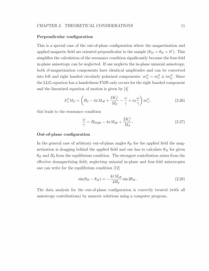
Perpendicular configuration
This is a special case of the out-of-plane configuration where the magnetization and
applied magnetic field are oriented perpendicular to the sample (θM = θH = 0). This
simplifies the calculation of the resonance condition significantly because the four-fold
in-plane anisotropy can be neglected. If one neglects the in-plane uniaxial anisotropy,
both rf-magnetization components have identical amplitudes and can be converted
into left and right handed circularly polarized components: mrf± = mrf
x ± imrfy . Since
the LLG equation has a handedness FMR only occurs for the right handed component
and the linearized equation of motion is given by [4]
hrf+MS =
(H0 − 4πMeff +
2K⊥1
MS
− ω
γ+ iα
ω
γ
)mrf
+, (2.26)
this leads to the resonance condition
ω
γ= HFMR − 4πMeff +
2K⊥1
MS
. (2.27)
Out-of-plane configuration
In the general case of arbitrary out-of-plane angles θH for the applied field the mag-
netization is dragging behind the applied field and one has to calculate θM for given
θH and H0 from the equilibrium condition. The strongest contribution arises from the
effective demagnetizing field; neglecting uniaxial in-plane and four-fold anisotropies
one can write for the equilibrium condition [12]
sin(θH − θM) = −4πMeff
2H0
sin 2θM . (2.28)
The data analysis for the out-of-plane configuration is correctly treated (with all
anisotropy contributions) by numeric solutions using a computer program.

CHAPTER 2. THEORETICAL CONSIDERATIONS 12
2.4 Physical Origin of Intrinsic Spin Damping
There are three major mechanisms which can cause intrinsic damping in metallic
ferromagnets. These are (i) eddy currents, (ii) magnon-phonon coupling, and (iii)
itinerant electron relaxation. In the following subsections all three mechanisms will
be examined with respect to their relevance to ultrathin metallic ferromagnets.
2.4.1 Eddy current mechanism
The precession of the magnetization induces eddy currents, and the dissipation of
them is proportional to the conductivity of the sample. For samples that are thinner
than the skin depth, the contribution of eddy currents to the equation of motion can
be evaluated by integrating Maxwell’s equations across the film thickness tF . The
resulting effective field has a Gilbert like form with an effective Gilbert damping
constant [13]
αeddy =1
6MSγ
(4π
c
)2
σt2F . (2.29)
where σ is the electrical conductivity. This contribution becomes comparable to the
intrinsic damping for samples thicker than 50 nm. The skin depth for Fe at a frequency
of 24 GHz is δ ∼ 100 nm. The thickest sample considered in this thesis was only 5
nm thick, hence the eddy current damping can contribute only ∼ 1% of the total
damping.
2.4.2 Phonon drag mechanism
Direct magnon-phonon scattering is another possible relaxation mechanism. Suhl re-
cently presented calculations for magnon relaxation by phonon drag [14]. His explicit
results are applicable to small geometries where magnetization and lattice strain are
homogeneous. Using the LLG and lattice strain equations of motion one can asymp-
totically describe the Gilbert phonon damping αphonon by [14]
αphonon =2ηγ
MS
(B2(1 + ν)
E
)2
, (2.30)
where η is the phonon viscosity, B2 is the magneto-elastic shear constant, E the Young
modulus, and ν is the Poisson ratio. All parameters can be readily obtained except
for the phonon viscosity η. Fortunately, the phonon viscosity parameter η for Ni

CHAPTER 2. THEORETICAL CONSIDERATIONS 13
in the microwave range of frequencies was experimentally determined in microwave
transmission experiments by Heinrich et al. [15]. In these studies at 9.5 GHz, a fast
transverse elastic shear wave was generated by magneto-elastic coupling inside the skin
depth of a thick Ni(001) crystal slab. This transverse elastic shear wave propagated
across the slab, and then reradiated microwave power at the other side of the Ni
slab. The effect was called ‘phonon assisted microwave transmission’. By fitting the
experimental data to the LLG and elastic wave equations of motion including the
magneto-elastic coupling, the elastic wave relaxation time was found to be τph =
6.6 × 10⁻¹⁰ s at 9.5 GHz. The phonon viscosity, as introduced in [14], is given by
η = c44/(τphω2), where c44 is the elastic modulus. For Ni η = 3.4 (in CGS units).
Using Eq. 2.30 results in a phonon Gilbert damping of αphonon ∼ 1 × 10⁻³ which
is ∼ 30 times smaller than the intrinsic Gilbert damping parameter of Ni. Since
magnetostrictive effects are stronger in Ni than in Fe, Co, or Py, it is expected that
the phonon drag mechanism will be even weaker in Fe, Co, and Py.
2.4.3 Itinerant electron mechanisms
The most important damping mechanism in ultrathin metallic ferromagnets is based
on itinerant electrons. The original model proposed by Heinrich et al. [16, 17] was
based on the interaction of s-p like electrons with localized d spins.
s-d interaction: spin-flip scattering
The s-d exchange interaction was calculated by integrating the s-d exchange energy
density [18]. The particle representation of the s-d exchange interaction Hamiltonian
for the rf-components of the magnetization is given by three particle collision terms
Hsd =
√2S
N
∑k
J(q)ak,↑a†k+q,↓bq + h.c., (2.31)
where S is the spin, N is the number of atomic sites, a† and a respectively create and
annihilate electrons, and b† and b create and annihilate magnons. The total angular
momentum and wave vector are conserved in the 3 particle collisions. ↑, ↓ stand for
majority and minority electrons, respectively. Itinerant electrons and magnons are
coherently scattered by the s-d exchange interaction resulting in the creation and
annihilation (h.c. term in Eq. 2.31) of electron-hole pairs as illustrated in Fig. 2.2.
Due to conservation of the angular momentum, the itinerant electron has to flip its

CHAPTER 2. THEORETICAL CONSIDERATIONS 14
ωq
εσk
εσ′k+q
Figure 2.2: A spin wave with energy ωq and momentum q collides with an electron in
state εσk changing its spin and momentum state to εσ′
k+q.
spin when it is scattered by a magnon. This coherent scattering on its own leads only
to a renormalized g-factor [16]. In order to cause relaxation, the electron-hole pair
needs to be incoherently scattered by thermally excited phonons or magnons. Such
incoherent scattering can be accounted for by introducing a finite life time τeff for the
electron-hole pair excitation [16]
δε = ε↓k+q − ε↑k + i
τeff
. (2.32)
τeff is given by the spin-flip time of the electron-hole pair τsf . τsf is longer than the
momentum relaxation time τm which determines the conductivity. For simple metals
Elliott [19] showed that this enhancement is related to the deviation of the g-factor
from the free electron value due to spin-orbit interaction
τsf
τm
=1
(g − 2)2. (2.33)
More reliable estimates for τsf can be obtained from measurements of the spin diffusion
length lsd. Giant magneto-resistance (GMR) experiments with the current flowing
perpendicular to the plane (CPP) allow one to estimate lsd by measurement of GMR
as a function of the magnetic layer thickness [20]. τsf and lsd are directly related by
[20, 21]:
τsf =6l2sdvF
λ↑ + λ↓λ↑λ↓
, (2.34)
where vF is the Fermi velocity and λ↑ and λ↓ are the electron momentum mean free
paths for spin up and spin down electrons. λm = 2λ↑λ↓
λ↑+λ↓= vF τm is the average
electron momentum mean free path of the ferromagnet. λm can be determined from
the resistivity [20]
=mvF
ne2
λm
1 − β2, (2.35)

CHAPTER 2. THEORETICAL CONSIDERATIONS 15
FM g lsd[nm] β [µΩcm] τsf [ps] G[107Hz] α[10−3] MS [ emucm3 ]
Fe 2.09 [22] 9.7 [23] 5.8 [24] 2 1710 [25]
Co 2.18 [22] 59 [26] 0.36 6.2 [23] 3.8 [20] 30 [27] 11 1425 [25]
Ni 2.21 [28] 6.8 [23] 25 [28] 19 485 [25]
Py 2.14 [29] 4.3 [20] 0.73 [20] 12.3 [20] 0.03[20] 9 6 860 [25]
MnNiSb 2.03 [30] 1 3.1 [30] 2.8 580 [30]
Table 2.1: Table showing the spin relaxation times and other relevant quantities for several
ferromagnetic materials (FM).
where β is the bulk spin asymmetry coefficient, m is the electron mass, and n is
the total conduction electron density of the ferromagnet. In Permalloy (Ni80Fe20, Py)
Py = 12.3 µΩ, βPy = 0.73, vF =1.5×108 cm/s, and n = 6.3×1022 cm−3 corresponding
to one conduction electron per atom [20]. The spin diffusion length in Py is lPysd = 4.3
nm [20] which with the aid of Eqs. 2.34 and 2.35 leads to τPysf = 3 × 10⁻¹⁴ s. A
short spin diffusion length implies that the spin scattering enhancement factor τsf/τm
is only ∼ 19 for Py. In Co similar GMR measurements [20] lead to lCosd = 59 nm at
77 K and require τCosf = 3.8 × 10⁻¹² s. In this case the corresponding spin scattering
enhancement factor is ∼ 300. By simply applying Eq. 2.33, one obtains τsf/τm ∼ 21
and ∼ 35 for Py and Co respectively. This means that Elliott’s formula predicts
the spin scattering enhancement factor correctly for Py but is wrong by an order of
magnitude for Co.
The rf susceptibility can be calculated using the Kubo Green’s function formalism
in the Random Phase Approximation (RPA) [31]. The imaginary part (damping) of
the denominator of the circularly polarized rf susceptibility is usually expressed as an
effective damping field [16]
αs−dω
γ=
2 〈S〉NgµB
∑k
|J(q)|2(n↓
k+q − n↑k
)δ(ωq + εk↑ − ε↓k+q), (2.36)
where the summation is carried out over all available states on the Fermi surface and
〈S〉 is the reduced spin 〈S〉 = S(MS(T )/MS(0)). The factor gµB = γ was used to
convert the relaxation energy into an effective relaxation field and δ is Dirac’s delta
function. The incoherent scattering of electron-hole pair excitations broadens the
delta function in Eq. 2.36 into a Lorentzian [16]
δ(ωq + ε↑k − ε↓k+q) /τsf
(ωq + ε↑k − ε↓k+q)2 + (/τsf)2
. (2.37)
CHAPTER 2. THEORETICAL CONSIDERATIONS 16
The difference in occupation numbers is ∆n = n↑k+q − n↓
k = δ(εk − εF )ωq, where
εF is the Fermi energy. The delta function keeps the relaxation processes limited to
electrons at the Fermi level. The energy ωq = ω of a resonant magnon is the energy
that is involved in the scattering process. One should view the Lorentzian function in
Eq. 2.37 not as a smeared energy conservation, but rather as probability distribution to
achieve a certain scattering event. FMR experiments are usually sensitive to the nearly
homogeneous mode, q ∼ 0 and the change in the energy for the spin-flip electron-hole
pair excitations is dominated by the exchange energy, ε↓k+q− ε↑k = −2 〈S〉 J(0). Using
N 〈S〉 gµB=Ms(T ) one obtains a damping field proportional to the frequency ω and
inversely proportional to the saturation magnetization MS. These are exactly the
features of Gilbert damping (see Eq. 2.8). After integration over the Fermi surface
one can extract the Gilbert damping parameter
αs−d =χp
MSγ
1
τsf
, (2.38)
where χp is the Pauli susceptibility for itinerant electrons. χp can be calculated from
the following expression
χp =
(γ
2π
)2 ∫k2dkδ(εk − εF ) = µ2
BN(εF ) , (2.39)
where N(εF ) is the density of states at the Fermi level. χp for 3d transition metals
is in the range of 3 − 9 × 10⁻⁶ [32]. An uncertain point, however, is the relationship
between τsf obtained from GMR measurements, see Eq. 2.34, and the τsf applicable
to magnetic relaxation rate (see Eq. 2.38). In GMR one measures the longitudinal
spin accumulation, while in FMR the transverse motion is relevant. The transverse
and longitudinal spin relaxation times must be closely related, but could differ by a
factor of 2. In ESR often the longitudinal relaxation is assumed to be 2 times slower
than the transverse relaxation time [33]
1
τsf
=1
T1
=1
2T2
. (2.40)
In order to obtain the Gilbert damping constant from Eq. 2.38, in the experimentally
observed range of α ∼ 5× 10⁻³ one needs to have τsf in the range of 5×10⁻¹⁴ s. This
is satisfied for Py, see Tab. 2.1. Ignoring the presence of collisions with thermally
excited magnons, the s-d relaxation is indirectly proportional to τm, and consequently
scales with resistivity. In fact, recently Ingvarsson et al. [34] showed that the Gilbert

CHAPTER 2. THEORETICAL CONSIDERATIONS 17
damping parameter in Py films can scale with the sample resistivity in agreement
with Eq. 2.38. Py, however, is a special case in that respect; in pure materials like
Co, Fe, and Ni the spin-flip relaxation time is too long and the s-d interaction hardly
contributes to Gilbert damping.
The above calculations were carried out for circularly polarized magnons. It was
shown that the ellipticity of magnons (in the parallel configuration) [35] does not
change the intrinsic Gilbert damping which is based on scattering processes, as shown
in Fig. 2.2. This result is not surprising considering that the FMR linewidth ∆H for
circularly polarized magnons showed the explicit feature of Gilbert damping, ∆H ∼1
MS
ωγ.
Spin orbit Hamiltonian: scattering without spin-flip
Kambersky [36] has shown that the intrinsic damping in metallic ferromagnets can be
treated more generally by using a spin-orbit interaction Hamiltonian. The spin-orbit
Hamiltonian for transverse spin and angular momentum components can be expressed
in a three particle interaction Hamiltonian
Hso =1
2
√2S
Nξ∑k
∑µ,ν,σ
〈µ|L+|ν〉c†ν,k+q,σcµ,k,σbq + h.c., (2.41)
where ξ is the coefficient of spin-orbit interaction, L± = Lx ± iLy are the right and
left handed components of the atomic site transverse angular momentum L. cµ,k,σ
and c†ν,k+q,σ annihilate and create electrons in the appropriate Bloch states with spin
σ, and bq annihilates a spin wave with the wave-vector q. The indices µ, ν represent
the projected local orbitals of Bloch states, and are used to identify the individual
electron bands. For simplicity the dependence of the matrix elements 〈ν|L+|µ〉 on
the wave-vectors is neglected. The rf susceptibility can again be calculated using the
Kubo Green’s function formalism in RPA. The imaginary part of the denominator
of the circularly polarized rf susceptibility for a spin wave with the wave vector q
and energy ω can be expressed in a manner similar to that for the s-d exchange
interaction. The effective damping field is then given by
αsoω
γ=
〈S〉22Ms
ξ2
(1
2π
)3 ∫d3k
∑µ,ν,σ
⟨ν|L+|µ⟩ ⟨µ|L−|ν⟩
× δ(εµ,k,σ − εF )ω/τm
(ω + εµ,k,σ − εν,k+q,σ)2 + (/τm)2. (2.42)

CHAPTER 2. THEORETICAL CONSIDERATIONS 18
Since no spin-flip occurs during the scattering event, the relaxation time τsf in Eq. 2.37
is replaced by the momentum relaxation time τm which enters the conductivity of the
ferromagnet.
Intraband transitions (µ = ν)
For small wave vector spin waves (q kF ) the electron energy balance ω + εµ,k,σ −εµ,k+q,σ = ω − (2/2m) (2kq + q2) in the denominator of Eq. 2.42 is significantly
smaller than /τm. In good crystalline structures this limit is satisfied above cryogenic
temperatures. After integration over the Fermi surface, the Gilbert damping can be
approximated by
αintraso 〈S〉2
MSγ
(ξ
)2(∑
µ
χµp
⟨µ|L+|µ⟩ ⟨µ|L−|µ⟩
)τm , (2.43)
where the χµp corresponds to the Pauli susceptibility of the given Fermi sheet. The
Gilbert damping in this limit is proportional to the electron momentum relaxation
time τm, and consequently scales with the conductivity.
Interband transitions (µ = ν)
The energy gaps ∆εν,µ correspond to interband transitions and the electron-hole pair
energy can be dominated by these gaps. For energy gaps larger than the momentum
relaxation frequency /τm the Gilbert damping constant can be approximated by
αinterso 〈S〉2
MSγ
∑µ
χµp (∆gα)2 1
τm
, (2.44)
were ∆gα = 4ξ∑
β 〈µ|Lx|ν〉 〈ν|Lx|µ〉 /∆εν,µ determines the contribution of the spin
orbit interaction to the g-factor [37]. If the spin-flip relaxation time τsf is obtained from
Eq. 2.33 the spin-orbit interaction results in a Gilbert damping coefficient similar to
that found for the s-d exchange interaction, as can be seen in Eq. 2.38. χµp only includes
those electron states for which the change in energy during the interband transition is
much bigger than /τm, i.e. ∆ε /τm. In this approximation the Gilbert damping
constant is proportional to 1/τm, and consequently scales with the resistivity. In
reality, the distribution of energy gaps determines the overall temperature dependence
of the Gilbert damping constant. Interband damping is expected to scale with the
resistivity only at low temperatures. With increasing temperature the relaxation rate

CHAPTER 2. THEORETICAL CONSIDERATIONS 19
/τm becomes comparable to the energy gaps, ∆εµ,ν , resulting in a gradual saturation
of αinterso [36].
Classical picture
Kambersky’s model was motivated by the observation that the Fermi surface changes
slightly when the magnetization is rotated [38]. This corresponds to intraband tran-
sitions and can be described by a classical picture. As the precession of the mag-
netization evolves in time and space, the Fermi surface distorts periodically in time
and space. This is often referred to as a breathing Fermi surface. The effort of the
electrons to appropriately repopulate the changing Fermi surface is delayed by their
momentum relaxation time τm and results in a phase lag between the Fermi surface
distortions and the precessing magnetization. On the other hand, the interband tran-
sitions lead to a dynamic orbital polarization, i.e. changes of the orbital electron wave
functions in addition to changes of the itinerant electron energies.
The s-d exchange interaction can be viewed as two precessing magnetic moments
corresponding to the localized d and itinerant s electrons, which are mutually cou-
pled by the s-d exchange field. In the absence of damping the low energy excitation
(acoustic mode) corresponds to a parallel alignment of the magnetic moments pre-
cessing together and in phase. Due to the finite spin mean free path of the itinerant
electrons, their equation of motion has to include the spin relaxation towards the
direction of the instantaneous effective field,
− 1
τsfγ(m − χPheff) , (2.45)
where heff also includes the exchange field between the localized and itinerant elec-
trons. This leads to a phase lag between the two precessing magnetic moments (s
and d) [39], and consequently to magnetic damping. The magnetic damping obtained
by means of this classical approach is equivalent to that obtained using the Kubo
formalism, as described above.
The phase lag for the breathing Fermi surface and the s-d exchange interaction
is proportional to the microwave angular frequency ω. Clearly, in both cases one has
‘friction’ like damping, which is described by Gilbert relaxation terms.

CHAPTER 2. THEORETICAL CONSIDERATIONS 20
Experimental evidence
In Ni the Gilbert damping increases significantly as the temperature is lowered from
room temperature (RT) and saturates for temperatures less than 50 K [40]. The
Gilbert damping parameter α was found to be 2.8 × 10⁻² at RT, and 16 × 10−2
at 4 K [40]. Korenman and Prange [41] explained the saturation of α using an
equation similar to Eq. 2.42. For intraband electron-hole pair excitations one has:
εk − εk+q = (kFq/m + q2/2m)2. With increasing τm the energy balance in the
denominator of Eq. 2.42 eventually becomes comparable to /τm. Both, momentum
and energy conservation now play an important role in the sum over the Fermi surface
in Eq. 2.42, and one finds
α ∼ tan−1 (qvFτm)
qvF
, (2.46)
where q is the wave number of a resonant magnon. For vFτm 1/q this expres-
sion saturates and depends inversely on q. This behavior has also been observed in
connection with the anomalous skin depth, where only electrons moving within the
skin depth contribute to the effective conductivity, and is usually referred to as the
concept of ineffective electrons [42]. The importance of ineffective electrons to the
Gilbert damping measured at low temperatures shows explicitly that the magnetic
damping in metallic ferromagnets is caused by itinerant electrons. This is further
supported by the results of Ferromagnetic Antiresonance (FMAR) experiments. By
using microwave transmission at FMAR (q → 0) one can avoid problems related to
the ineffective electrons [43] and obtain precise values of the intrinsic damping. Hein-
rich et al. found that in high purity single crystal slabs of Ni the Gilbert damping
below RT was well described by two terms, one of which was proportional to the con-
ductivity, the other proportional to the resistivity [43]. At RT these two terms were
approximately equal in strength and compensated each other resulting in a nearly
temperature independent Gilbert damping parameter [28]. This is in agreement with
the above predictions. The saturation of the damping parameter above RT is quite
well accounted for in quantitative calculations by Kambersky [44] and is explained by
the interband contributions which saturate above RT.
Summary
FMR measurements in high quality crystalline Ni samples convincingly showed that
the intrinsic damping in metals is mostly caused by the itinerant nature of the elec-

CHAPTER 2. THEORETICAL CONSIDERATIONS 21
trons and the spin-orbit interaction. Quantitative calculations [16, 36, 44, 45, 46]
identified the spin-orbit interaction as the leading intrinsic damping mechanism in
ferromagnetic metals.

CHAPTER 2. THEORETICAL CONSIDERATIONS 22
2.5 Extrinsic Damping: Two-Magnon Scattering
It was shown in section 2.4.3 that intrinsic damping results in a resonance linewidth
which is linearly proportional to the microwave frequency. Experimentally, however,
the linewidth is often found to have a linear frequency dependence with an extrapo-
lated non-zero linewidth for zero frequency (∆H(0)) [47]. Consequently, the measured
linewidth versus frequency is often interpreted using the simple relationship
∆H(ω) = ∆H(0) + αω
γ, (2.47)
where the linear term is assumed to be a measure of the intrinsic damping and the
magnitude of ∆H(0) depends on the film quality and approaches zero for the best
samples. This implies that ∆H(0) is extrinsic and is caused by defects. In the
model of extrinsic damping by two-magnon scattering a uniform precession magnon,
q ∼ 0 (FMR mode), scatters into q = 0 magnons. Energy conservation requires
that the resonant mode (q ∼ 0) can only scatter into spin waves oscillating at the
same frequency i.e. ω(0) = ω(q). q is determined by the magnon dispersion relation.
Momentum conservation is not required due to the loss of translational invariance.
This mechanism was envisioned four decades ago to explain the extrinsic FMR line
broadening in YIG spheres [48]. Since then magnon scattering has been extensively
used to describe extrinsic damping in ferrites [49, 50, 51, 52, 53]. Patton and co-
workers pioneered this concept in metallic films [54].
The two-magnon scattering matrix is proportional to components of the Fourier
transform of the magnetic inhomogeneities A(q) =∫
dr∆U(r)e−iqr, where U(r)
stands symbolically for a local anisotropy energy. In ultrathin films the magnon
q vectors are confined to the film plane (i.e. q = q‖).
Recently, Arias and Mills [12] introduced a theory of two-magnon scattering that
applies to ultrathin films. For arbitrary azimuthal angles and neglecting magneto-
crystalline anisotropies the spin wave dispersion relation has the form [12]
ω2
γ2=
ω2hom
γ2− 2πMSq‖tF[sin2 θM − cos2 θM cos2 ψq][H0 cos(θH − θM)
− 4πMeff sin2 θM ] − sin2 ψq[H0 cos(θH − θM) − 4πMeff cos 2θM ]+ Dq2
‖[2H0 cos(θH − θM) + 4πMeff(1 − 3 cos2 θM)], (2.48)
where D = 2A/MS is the spin wave stiffness constant and ψq is the angle between the
in-plane projection of the static magnetization and the propagation direction of the

CHAPTER 2. THEORETICAL CONSIDERATIONS 23
spin wave with wave vector q‖ in the sample plane. ωhom is the resonance frequency
of the homogeneous precession of the magnetization and is given by
ω2hom
γ2= [H0 cos(θH − θM ) − 4πMeff sin2 θM ][H0 cos(θH − θM ) + 4πMeff cos 2θM ]. (2.49)
In the parallel FMR configuration the second term on the right hand side of Eq. 2.48
is negative and proportional to q‖, and therefore it lowers the resonance frequency
for magnons with q‖ > 0 (see Fig. 2.3a). For bigger q‖ vectors, the third term
in Eq. 2.48 increases the magnon energy again due to the exchange field, and the
magnon dispersion curve crosses the the energy of the homogeneous precession of the
magnetization at a magnon wave vector q0‖(ψq). This means that the homogenous
FMR mode is degenerate with the q0‖(ψq) mode (see Fig. 2.3a) and can be involved
in two-magnon scattering. By inspection of Eq. 2.48 one can also see that when
the magnetization is tipped out of the plane at angles smaller than θM = π/4, no
degenerate magnons are available (in this case the second term in Eq. 2.48 becomes
positive and the spin wave energy can never be lower than or equal to the energy of
the homogeneous mode).
The value of q0‖(ψq) decreases with increasing angle ψq between q‖ and M, as
shown in Fig. 2.3b. No degenerate modes are available for an angle ψq larger than
[12]
ψmax = arcsin
(HFMR
H + 4πMeff
) 12
, (2.50)
where HFMR is the field at FMR.
Arias and Mills developed a detailed theory for the case that the magnetization
and applied field are parallel to each other and confined to the film plane [12]. Their
quantum mechanical theory was based on a response (Green’s) function formalism
and a continuum approach [55]. The response functions were defined as
Sαβ = iθ(t)
〈[mα(q‖, t),m
†β(q′
‖, 0)]〉, (2.51)
where the mα,β(q‖, t) are operators for the transverse magnetization components. A
magnon-magnon scattering potential was introduced in the most general way
V =∑q′‖,q‖
1
2m†
x(q′‖)Vxx(q
′‖,q‖)mx(q
′‖) + m†
x(q′‖)Vxy(q
′‖,q‖)my(q
′‖) (2.52)
+1
2m†
y(q′‖)Vyy(q
′‖,q‖)my(q
′‖).
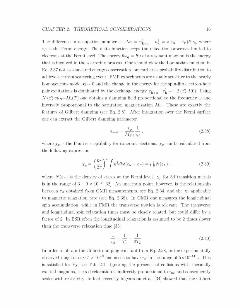
CHAPTER 2. THEORETICAL CONSIDERATIONS 24
Figure 2.3: (a) Calculated spin wave dispersion spectra for a 30 ML thick Fe film at a
frequency of 24 GHz. Here ψq = 0, where ψq is the in-plane angle between the magnetization
and wave vector q‖. The various curves correspond to a magnetic field inclined by 1 steps
from the in-plane configuration (lowest spectrum, θH = θM = 90) to the perpendicular
configuration (highest spectrum, θH = θM = 0). The q0‖ wave vectors for degenerate
magnons are given by the intersection with the dashed line. (b) Shows the dependence of
q0‖(ψq) on θH . Note that the degenerate magnons are lost for θH ≤ 15 which corresponds
to θM ≤ π/4.
For the case relevant to the FMR mode (q‖ = 0) one can show that the susceptibility
is given by [12]
Sxx =(H0 + 4πMeff)MS(
ωhom
γ
)2 − (ωγ
)2 − iαωγ[Meff + 2H0] − R2m
, (2.53)
were R2m is the additional relaxation parameter due to two-magnon scattering and
defined as
R2m ≡ πγ4M2S
2ωhom
∑q
∣∣∣(4πMeff + H0)Vxx(0,q‖) + H0Vyy(0,q‖) (2.54)
+ i[H0(4πMeff + H0)]12 [V xy(0,q‖) − V xy(0,q‖)]
∣∣∣2δ[ω(q‖) − ωhom].
The imaginary part of R2m is responsible for the two-magnon relaxation and provides
additional damping of the FMR mode, while the real part of R2m shifts the resonance
field slightly. In order to calculate the strength and frequency dependence of two-
magnon scattering, Arias and Mills [12] evaluated the matrix elements Vαβ by using

CHAPTER 2. THEORETICAL CONSIDERATIONS 25
3 different sources of perturbation: (i) spatially inhomogeneous Zeeman energy, (ii)
spatially inhomogeneous dipolar energy, and (iii) spatial variation of the perpendicular
uniaxial anisotropy axis [12]. Only (iii) was found to produce a sizable two-magnon
effect. The inhomogeneities were assumed to have a rectangular shape with lateral
dimensions a and c and a random size distribution between 1 and Na, Nc. After a
series of complicated algebraical steps it was shown that the two-magnon contribution
to the FMR linewidth can be written as [12, 56]
∆H2m =32(K⊥
U )2b2p
πM2S
√3D
sin−1
(H0
2H0 + 4πMeff
)[〈ac〉 − 1
], (2.55)
where p is the fraction of the surface area covered by defects, and b is the average
defect height. This calculation allows one to refine the empirical formula Eq. 2.47 by
the replacement of ∆H(0) by ∆H2m from Eq. 2.55.
CHAPTER 2. THEORETICAL CONSIDERATIONS 26
2.6 Magneto-Optic Kerr Effect
Magneto-optic effects change the polarization of light by interaction with magnetized
matter. This effect was dicovered by John Kerr in 1877 [57, 58] and is called the Kerr
effect. The plane of polarization of incoming linearly polarized light rotates slightly by
an angle θk and becomes elliptically polarized upon reflection from a magnetic sample.
The origin of the Kerr effect is briefly discussed below in terms of the Lorentz model.
In the macroscopic theory the magneto-optic properties of a material can be de-
scribed by the dielectric permittivity tensor ←→ε . For magnetic media this tensor has
off-diagonal elements, the magnitude of which is proportional to the magnetization.
The permittivity tensor for an isotropic magnetic medium can be written as
←→ε = ε0
1 −iQvαZ iQvαY
iQvαZ 1 −iQvαX
−iQvαY iQvαX 1
, (2.56)
where ε0 is the dielectric constant, Qv is the Voigt coefficient (proportional to MS),
and αXY Z are direction cosines of the magnetization. The Maxwell equation relating
the vectors of the electric displacement density D and the electric field strength E
can be written as
D = ←→ε E = ε0(E + iQvm × E). (2.57)
where m is a unit vector aligned with the magnetization. The polarization vector of
the light therefore rotates around the magnetization.
There are three principal configurations for Kerr effect measurements, as shown
in Fig. 2.4. These configurations differ in their relative orientation of the light po-
larization, magnetization, and film plane. They are: (i) Polar configuration, the
magnetization points normal to the sample plane and the light polarization lies in
the sample plane; (ii) Longitudinal configuration, the magnetization is in-plane and
parallel to the plane of incidence; and (iii) Transverse configuration, the magnetiza-
tion is in the sample plane and oriented perpendicular to the plane of incidence. To
understand the origin of the Kerr effect classically one can consider the equation of
motion for electrons in an harmonic (crystal) potential driven by the electric field of
the incident light
mx + mω20x = eE0e
iωt + e(x × B), (2.58)

CHAPTER 2. THEORETICAL CONSIDERATIONS 27
M
v
M
v Mv
polar longitudinal transverse
Figure 2.4: Polar, longitudinal, and transverse configurations for Kerr effect measurements.
The arrows inside the circles represent the direction of the electric vector E of linearly
polarized light. The rotation of the polarization and the intensity change due to the Kerr
effect is illustrated by the darker arrow on the reflected light side. ν indicates the direction of
the Lorentz force exerted on the moving electrons inside the magnetic medium (ν ‖ M×E).
EE
M
k
k
Sample
Figure 2.5: Longitudinal configuration illustrating the meaning of the Kerr angles θk and
εk. The reflected light can be split into a linearly polarized in-phase component (ϕ = 0)
with rotation angle θk and an elliptically polarized out-of-phase component (ϕ = π/2) with
ellipticity angle εk.
where x is the electron displacement and ω0 is the angular frequency of the incoming
light. It is assumed that the light polarization E0 is in the film plane and E0 ‖ x. The
Lorentz force on the right hand side of Eq. 2.58 is in the plane of the surface if B is
perpendicular to the surface (B ‖ z). This corresponds to the polar configuration, see
Fig. 2.4a. Therefore the polarization of the reradiated (reflected) light will be rotated.
Similar arguments apply to the other Kerr configurations.
The true microscopic origin of the magneto-optic effect lies in exchange and spin-

CHAPTER 2. THEORETICAL CONSIDERATIONS 28
orbit coupling which gives rise to a large effective field in the direction of M. This
field leads to a Lorentz force and rotates the polarization. The light reflected from
the metallic sample only interacts with a thin surface layer whose thickness is given
by the skin depth. For metals the skin depth is of the order of 100 A in the visible
light spectrum. Hence the Kerr rotation of the polarization is very small and usually
only of the order of 10−3 degrees.
Since the permittivity tensor is complex the Kerr signal is measured by two quan-
tities: rotation angle θk and ellipticity angle εk. Their definition is shown in Fig. 2.5.
In the polar Kerr configuration θk and εk are roughly 10 times bigger than in the
longitudinal configuration. This is due to the large refractive index (sum of real and
imaginary parts) of metals which causes the effective angle of incidence to be small
(typically 5-8). In this case the light propagates mostly perpendicular to the magne-
tization and the component of the Lorentz force which is perpendicular to the electric
field is small.

Chapter 3
Experimental Methods
In this chapter the ultra-high vacuum (UHV) system that was used for sample prepa-
ration and the techniques that were employed in the magneto-dynamic studies are
discussed. The chapter starts with a detailed description of the UHV system and
associated techniques used for film growth and characterization. The second part
of this chapter will address the Ferromagnetic resonance (FMR) and magneto optic
Kerr effect (MOKE) technique which were employed in static and dynamic magnetic
measurements.
3.1 The Ultra-High Vacuum System
Epitaxial metallic films were prepared in UHV by means of molecular beam epitaxy
(MBE). The UHV system is composed of 4 interconnected chambers, as illustrated in
Fig. 3.1. (a) The intro chamber was used for outgassing and hydrogen cleaning after
the samples were introduced into UHV from the load lock. (b) The analysis chamber
houses an apparatus for Auger electron spectroscopy (AES), X-ray photo emission
spectroscopy (XPS), and ultraviolet photoemission spectroscopy (UPS). These tools
permit atomic and chemical characterization of the sample surface. In addition an
Ar+ ion gun in the analysis chamber allows one to remove surface contaminants and
to conduct depth profile analysis. (c) The growth chamber has 8 thermal evaporation
furnaces embedded in a cryo-shroud. The atomic surface topography and growth
rate were monitored using reflection high energy electron diffraction (RHEED) and
a quartz crystal micro balance. (d) The SPM chamber accommodates an Omicron
large area scanning probe microscope (SPM) which includes a scanning tunnelling
29

CHAPTER 3. EXPERIMENTAL METHODS 30
microscope (STM) and an atomic force microscope (AFM). The sample holder is
mounted on a linear transfer arm, and includes goniometers for adjustment of the
azimuthal and polar angles of the sample. The transfer arm has 130 cm of travel,
allowing one to move the sample between the various chambers. The sample can
therefore be oriented at arbitrary azimuthal and polar angles in all chambers. The
temperature of the sample substrate can be varied between −200 C and +700 C.
3.1.1 Substrate preparation
All samples were grown on single crystalline GaAs(001) wafers. Commercial epi-ready
GaAs substrates (manufactured by American Xtal Technology) are always covered by
a several nm of natural oxide. This oxide layer was removed under UHV conditions
using two techniques: (i) Ar+ ion bombardment and (ii) atomic hydrogen etching.
Both techniques have advantages and shortcomings, and are described below.
Ar+ sputtering
Samples are introduced into the intro UHV chamber via the small independently
pumped load lock chamber. This allows the pressure in the intro chamber to be held
at less then 1 × 10⁻⁸ torr during loading of a GaAs sample holder onto the UHV
goniometer. Subsequently, the GaAs substrates are outgassed at 400 C for several
hours until the base pressure in the intro chamber fell below 5×10⁻¹⁰ torr. The wafer
is then cooled down to RT and bombarded by 600 eV Ar+ ions at a grazing angle
(65 with respect to the surface normal) to remove surface contaminants. During
sputtering the sample is rotated around its normal and the ion beam was rastered
over the sample. The ion beam bombardment is imaged as a function of the beam x-y
deflection voltages. An image of the sample is acquired by measuring the ion current
flowing into one of the tungsten clips which are used to hold the wafer. During
ion bombardment the surface of an otherwise semi-insulating GaAs wafer becomes
conducting (probably due to the atomic disorder and site exchange doping AsGa)
allowing one to follow the position of the ion beam by monitoring the absorbed ion
current, as shown in Fig. 3.2. In this way it is possible to maximize the ion flux
over the sample by optimizing the ion-gun optics, sample position, and raster size.
In our differential ion gun, the Ar gas was bled directly into the ionization chamber
allowing one to maintain an Ar back-pressure of 3×10⁻⁷ torr during sputtering. While

CHAPTER 3. EXPERIMENTAL METHODS 31
Figure 3.1: Sketch of the UHV MBE system. The MBE system consists of four chambers:
(a) intro chamber (bottom right), (b) analysis chamber (top right), (c) growth chamber (top
left), (d) and SPM chamber (bottom left).
sputtering, the chamber was pumped by two 500 l/s turbo pumps. A clean surface
was obtained after 5 − 7 hours of sputtering depending on the thickness of the oxide
layer.

CHAPTER 3. EXPERIMENTAL METHODS 32
Figure 3.2: UHV sample holder with a 10×10 mm GaAs wafer held by two tungsten clips.
The inset on the left side shows an image of the GaAs wafer acquired by monitoring the
absorbed ion current during Ar+ sputtering, as discussed in the text.
H· cleaning
Atomic hydrogen provides a faster and easier way to remove surface contaminants.
During the cleaning procedure the sample temperature was held at 400 C. A hydrogen
doser (Oxford Scientific) thermally cracks hydrogen molecules into neutral atoms by
passing H2 gas through a narrow 2000 C hot tungsten tube; the tungsten tube is
heated by electron bombardment. H2 molecules are dissociated into atomic hydrogen
(H·) during collisions with the hot wall of the tube. This provides an atomic hydrogen
beam with about 15 degrees divergence and a cracking ratio H/H2 of up to ∼ 95%
[59]. Without atomic hydrogen the thermal desorption temperatures for Arsenic and
Gallium oxides on GaAs are 450 C and 580 C, respectively [60]. Atomic hydrogen
removes both oxides at 400 C.
The chemistry of the hydrogen surface cleaning process may be summarized as
follows [61, 62]: Arsenic oxides can be removed from the surface (↑) by H· cleaning in
the following reaction:
As2Ox + 2xH· → xH2O ↑ +As2 ↑, (3.1)
were x= 1, 3, or 5 stands for the various oxides of arsenic. Ga2O3 is decomposed as
Ga2O3 + 4H· → Ga2O ↑ +2H2O ↑ . (3.2)

CHAPTER 3. EXPERIMENTAL METHODS 33
LN2UHV H2
gas purifier
pressure regulatorcold trap
purge valve
hot capillary
leak valve
water cooling
Figure 3.3: Schematic view of the hydrogen doser.
Ga2O becomes volatile at temperatures greater than 200 C. If permitted to remain
on the surface Ga2O would act as an etch stop, or lead to a Ga-rich surface as a result
of the subsequent reaction
Ga2O + 2H· → 2Ga + H2O ↑, (3.3)
which is undesirable. Therefore, the temperature should not be chosen to be less than
350 C; greater than 400 C is preferable, allowing for rapid Ga2O desorption. It
has been shown that hydrocarbons and CO contaminants can also be removed using
atomic hydrogen [62]. Thus one can prepare a clean and stoichiometric GaAs surface
[61].
During cleaning the hydrogen back pressure is 5×10⁻⁷ torr. The ion pump in the
intro chamber was not used during cleaning because the hydrogen exposure leads to
the release of water from the ion pump electrodes. A liquid nitrogen cooled titanium
sublimator pump (TSP), however, inside the ion pump allows very efficient pumping
of hydrogen. The TSP housing in the intro chamber has an inner diameter of 10 cm
and is about 16 cm tall giving an internal area of about 500 cm2. At 77 K TSP has a
pumping speed for hydrogen of about 10 ls−1cm−2 [63]. The effective pumping speed
depends on the length and diameter of the pipe connecting the intro chamber to the
TSP. The conductance of this pipe in (ls−1) is given by [63]:
Cpipe = 3.81 ×√
T
M
(D3
L + 1.33D
)l
s, (3.4)
CHAPTER 3. EXPERIMENTAL METHODS 34
were T is the temperature (300 K), M is the molecular mass (for hydrogen), and
D(16 cm) and L(40 cm) are the pipe diameter and length, respectively. This yields a
pipe conductance of 2400 l/s. Therefore the effective TSP hydrogen pumping speed
is approximately 1600 l/s.
Using this pumping speed one can estimate the hydrogen pressure in the tungsten
tube and find the molecular hydrogen dissociation rate [59]. The tungsten capillary
has a diameter of D = 0.5 mm and a length of L = 5 cm, resulting in Ctube = 0.04 l/s;
the hydrogen dissociation takes place in the last 5 mm of tube [59]. During cleaning
the hydrogen pressure is pintro = 5×10⁻⁷ torr in the intro chamber and combined with
1600 l/s pumping speed requires a pressure of ptube 2 × 10⁻² torr in the hot tube
(steady state solution: ptubeCtube = pintro1600 l/s ). At this pressure the dissociation
rate of H2 is expected to be 90 %, assuming a tube temperature of 2000 K [59]. The
gas throughput Q is given by
Q = C(ptube − pchamber) = 0.04l
s(2 × 10⁻²) torr = 1.1 × 10⁻⁴ m3Pa
s. (3.5)
Using the ideal gas equation one can write
Q = pdV
dt= kBT
dN
dt dN
dt=
1.1 × 10⁻⁴
kBT
m3Pa
s= 3.8 × 10¹⁵ atoms
s. (3.6)
From the molar volume at RT and atmospheric pressure the corresponding amount
of hydrogen in cc is:
dV
dt
∣∣∣300K
1atm= 0.5
cc
hour. (3.7)
A time interval of 30 min was required for cleaning. This means that a volume of
0.25 cc of hydrogen (at atmospheric pressure) was used during cleaning. One can
estimate the number density of impinging hydrogen atoms on the sample surface and
their reaction probability. The nozzle of the tungsten capillary was at a distance
of 4 cm from the sample during cleaning and hence the hydrogen beam covered an
area of ∼ 4 cm2. Therefore only a quarter of the H· flux impinged on the 10 × 10
mm sample. Using Eq. 3.7 the number of hydrogen atoms hitting the GaAs wafer
in 30 min was N30minH = 1.7 × 10¹⁸ atoms. This number can be used to estimate the
reaction probability. Assuming 50 monolayers of oxide one gets ∼ 50 × 1015 oxide
sites resulting in a reaction probability of ∼ 3 %. This is only a crude estimate, but
the number seems very reasonable. In a more accurate calculation the ineffectiveness
of cleaning for a sub monolayer oxide coverage should be considered.

CHAPTER 3. EXPERIMENTAL METHODS 35
3.1.2 Electron spectroscopy
Auger electron spectroscopy (AES) and x-ray photoemission spectroscopy (XPS) allow
one to measure the elemental and chemical composition at the surface of a sample. In
these techniques an incident electron beam (AES) or an incident x-ray beam (XPS)
results in the emission of electrons from the sample surface. The kinetic energy
spectrum of the emitted electrons exhibits peaks that are element specific since the
energy of these electrons depends on the binding energy of the excited electron (XPS)
or on the energy difference between the specific atomic energy levels (AES) [64, 65].
Both techniques are surface sensitive because the electron mean free path is less than
2 nm in the relevant energy range (100 eV-2 keV) [66]. Hence only a 2 nm thick
surface layer of the sample can contribute to the signal. Using the UHV goniometer,
the angle of the analyzer with respect to the sample surface can be changed, which
further allows one to separate the bulk and surface contributions to the signal. XPS
is based on the analysis of the kinetic energy of electrons emitted from a surface in
response to a monochromatic x-ray beam (in our case Al-Kα, hν = 1486.6 eV or
Mg-Kα, hν = 1253.6 eV). The energy spectrum of emitted electrons was measured
by means of a hemispherical capacitive analyzer (SCA). The analysis chamber is
equipped with a Physical Electronics digital analyzer system (PHI 5400). The electron
energy spectrum is analyzed by sweeping the potential VA (see Fig. 3.4), thus shifting
the analyzer Fermi level relative to the sample Fermi level. Electrons are not used
as a primary beam in XPS because electron-electron scattering processes in solids
would result in a broad primary energy unsuitable for the analysis of the narrow XPS
peaks. In x-ray spectroscopy the primary energy is transferred to the photo electron,
and electron-electron scattering only plays a role when the photo electron leaves the
crystal. Energy conservation determines the kinetic energy (KE) of the photo emitted
electron,
KEXPS = hν − BE − φA, (3.8)
where BE is the core hole binding energy measured relative to the Fermi energy, as
illustrated in Fig. 3.4. In addition, the resulting core hole is eventually filled with an
electron originating from an outer shell. At the same time an Auger electron from
another shell is emitted, carrying away the excess energy. The AES kinetic energy
(KEAES) is given by
KEKLLAES = EBK − EBL2 − EBL3 − φA, (3.9)

CHAPTER 3. EXPERIMENTAL METHODS 36
Energ
y
2s (L )1
2p (L )2. 3
3s (M )1
3p (M )2, 3
Photo electron
Auger electron
KEXPS
1s (K)
h
EFS
hh BE - - -V A
KEKLL KE -KLL -VA
A
AnalyzerSpecimen
VA
A
EF
S
Figure 3.4: Energy level diagram for XPS and AES. KE and BE are the electron kinetic
energy and binding energy, respectively. φS,A are the sample and spectrometer work func-
tions. ESF, EA
F are the sample and analyzer Fermi levels, respectively. hν is the incident
photon energy. The energy levels of the sample are indicated in the left part. On the right,
the potential of the electron analyzer is shown relative to the sample potential on the left.
In electron spectroscopies the binding energy is measured with respect to the Fermi level.
Note that for the retarding potential VA = 0, the Fermi levels of the sample and the analyzer
are equal.
where the EB’s correspond to the appropriate electron level binding energies (see
Fig. 3.4). AES utilizes the element specificity of the binding energies. In AES the ini-
tial core hole is usually generated by high energy electrons originating from a primary
electron beam with a fixed energy (3keV in our system). Auger electrons, however,
are also present in XPS (see Fig. 3.4). The sensitivity of electron spectrometers allows
one to detect a surface coverage of ∼ 0.01 monolayer (ML).
During relaxation of the core hole the generation of Auger electrons and x-ray
fluorescence are competing processes for carrying away the excess energy. For light
elements the probability of generating Auger electrons is almost unity but with in-
creasing atomic number this probability drops dramatically. For atomic numbers
larger than 30, the x-ray fluorescence signal becomes larger than the Auger electron

CHAPTER 3. EXPERIMENTAL METHODS 37
metal chunks
Ta filament
1 cc crucible
Ta radiation shield
30 mm
Figure 3.5: Cross section of a MBE source.
signal. Therefore AES is a less sensitive technique for elements with large atomic
numbers when compared to XPS.
3.1.3 Metallic film growth
Metallic films were grown by means of molecular beam epitaxy (MBE) directly on
GaAs(001) templates. The molecular beam sources were based on thermal evaporation
in UHV and the growth rate was usually ∼ 2 ML/min. In all samples the first metallic
layer grown on GaAs(001) was Iron. Fe grows well on GaAs(001) [67] and has a lattice
spacing that is closely matched to the size of half a unit cell of GaAs(001). The
lattice mismatch of Fe to GaAs is only −1.4%. A crystalline epitaxial seed layer of
Fe(001) served as a template for the epitaxial growth of other metallic layers: Au(001),
Ag(001), Cu(001), Pd(001), and Cr(001).
Metal Sources
Fig. 3.5 shows the basic design of the evaporation sources used for the samples in this
thesis. A crucible filled with the desired metal was placed inside a multilayer tantalum
radiation shield and resistively heated by means of a tantalum filament having an
impedance of ∼ 0.5 Ω at a current of ∼ 40 − 60 A. All metal sources Ag(830 C),
Cu(1030 C), Fe(1180 C), Cr(1160 C), and Pd(1190 C) had an Alumina (Al2O3)
crucible except for Au(1130 C), which had a pyrolytic boron nitride (PBN) crucible.
PBN cannot be used for transition metals because they tend to react with PBN to

CHAPTER 3. EXPERIMENTAL METHODS 38
form N2 and nitrides when hot. The numbers in brackets listed with each of the
elements represent the temperature required to achieve a vapor pressure which is
sufficient for evaporation (∼ 10−3 torr). A Ta liner inside the alumina crucible was
used for the Ag and Cu furnaces in order to prevent stress induced cracking of the
crucible. All furnaces were surrounded by a liquid nitrogen cooled cyro shroud and
the copper power feed-throughs (2.5”) were water cooled. The cryo-shroud served to
absorb unwanted gas species originating from the hot furnaces during film growth.
Reflection high energy electron diffraction
Reflection High Energy Electron Diffraction (RHEED) is a powerful analytical tech-
nique which was used during the sample growth. It is a non-invasive tool that can
provide real-time information about surface morphology and symmetry. At the same
time it allows one to measure the thickness of the growing film with sub monolayer
accuracy. In this technique a 10 keV electron beam impinges on the sample surface
at a grazing angle of ∼ 1 (see Fig. 3.6). Due to the shallow angle of incidence,
very little momentum perpendicular to the surface is available and hence the elec-
tron beam interacts with only one or two atomic layers at the surface. On an ideal
surface this would result in diffraction from a two dimensional periodic mesh. The
three dimensional reciprocal lattice is replaced by rods due to the lack of scatterers
perpendicular to the surface. The diffracted beams are given by the intersection of
the Ewald sphere with the reciprocal rods [68] (see Fig 3.6). The electron energy is
chosen such that the Ewald sphere is large enough to intercept several reciprocal rods
having a spacing of 2π/a, where a is the in-plane atomic spacing. Hence RHEED
is sensitive to the periodicity of the surface lattice. The first order diffraction spots,
specularly reflected electrons, and the through beam lie on one circle, as illustrated in
Fig. 3.6. The diffracted and reflected electrons illuminate the phosphorescent screen,
and a digital charge coupled device (CCD) camera is used to monitor the diffraction
pattern and its time evolution during the sample growth.
Surface reconstruction of GaAs(001)
GaAs is an ionic crystal having zinc blende structure and a lattice constant of a =
5.654 A. The zinc blende structure corresponds to two interpenetrating fcc lattices
of Ga and As atoms shifted mutually along the [111] direction by 1/4 of the body
diagonal [69]. The bonding between atoms is ionic and covalent in character. An ideal

CHAPTER 3. EXPERIMENTAL METHODS 39
Figure 3.6: The geometry of RHEED. The Ewald sphere represents the k-space of electrons
having the same energy as the incident beam. The intersection of the reciprocal rods with
the Ewald sphere determines the diffraction beams. Low index diffraction beams intersect
the phosphorescent screen and provide information about the film surface symmetry and
roughness.
GaAs(001) surface would be either As or Ga terminated. The surface atoms, however,
do not have neighbors in the [001] direction and thus the GaAs001 plane would be
charged. In order to avoid a surface charge density, the equilibrium positions of the
surface atoms have to differ from the bulk. Which reconstruction occurs depends
upon temperature and surface stoichiometry. On the GaAs(001) surface the [110]
and [110] directions are not equivalent and the convention adopted is that in-plane
components of the Ga bonds are parallel to the [110] direction, and the in-plane
components of the As bonds are parallel to the [110] direction [70]. This uniaxial
property results in a magnetic uniaxial interface anisotropy for Fe films grown on
GaAs(001). Energy level calculations for GaAs(001) [71] predict that the As dangling
bond energy lies in the valence band (i.e. filled) and the dangling bond energy of Ga
lies above the conduction band (i.e. empty). This means that in order to minimize
the total energy, the surface electrons have to go from Ga to As [72]. This is achieved
by the formation of dimers at the surface and results in surface reconstructions which
can be identified by 2 numbers A×B, where A is the size of the unit cell (in units of

CHAPTER 3. EXPERIMENTAL METHODS 40
Figure 3.7: RHEED patterns of a hydrogen cleaned GaAs sample after annealing at 600 C.
Image (a) was recorded with the primary electron beam oriented along the [110] direction
and shows 5 satellite spots between the main diffraction spots characteristic of the 1 × 6
reconstruction. In (b) the primary electron beam was oriented along the [110] direction.
The 3 satellites between the primary spots correspond to the 2 × 4 reconstruction.
atomic spacings) in the [110] direction, and B is the size of the unit cell in the [110]
direction. With increasing temperature As is preferentially lost from the surface due
to its higher vapor pressure compared to Ga and the surface becomes Ga rich. The
following reconstructions sequenced from As-rich to Ga-rich are commonly found on
GaAs(001): (4 × 4), (2 × 4), (1 × 6), (2 × 4), and (8 × 2).
After the GaAs wafers were cleaned the surface was annealed while monitoring
the RHEED pattern. The wafer temperature was gradually raised to 600 C within
30 minutes. Under these conditions the atoms at the surface become mobile and form
domains of 4×2 and 6×1 surface reconstructions [67, 73, 74]. These reconstructions
represent additional periodicities of the surface and can be observed in RHEED.
Fig. 3.7 shows the diffraction patterns of a GaAs(001) wafer after annealing. The
surface consists of (1 × 6), and (2 × 4) reconstructed domains [73].
RHEED oscillations
When the angle of the incident electron beam θi is set up to correspond to the anti
Bragg condition, the measured intensity of the specular spot can oscillate during film
growth. Simple layer by layer growth can be described in a kinematic approximation
as proposed by van Hove et al. [75]. This model assumes that the electrons are

CHAPTER 3. EXPERIMENTAL METHODS 41
Figure 3.8: RHEED oscillations calculated from Eq. 3.11 with θi corresponding to the anti
Bragg condition.
scattered only from the topmost surface atomic layers 1 and 2. In perfect layer by
layer growth, the lower layer is always completely filled while the top layer coverage Θ
increases periodically from 0 to 1 during the film deposition. The diffracted electrons
scattered from atoms at level 1 and 2 have a relative phase shift ∆φ. Using Bragg’s
law
∆φ = 2|ki|a⊥ sin θi, (3.10)
where ki is the incident electron k-vector and a⊥ is the lattice spacing perpendicular
to the surface. The intensity of the specular spot is determined by the interference of
the scattered electron wave functions. The electron wave scattered from the top layer
will be proportional to the coverage ψ1 ∼ Θ and the wave from the bottom layer will
be proportional to ψ2 ∼ (1 − Θ)ei∆φ. This implies that the intensity of the specular
spot is proportional to
ISP ∼ |ψ1 + ψ2|2 ∼ Θ2 + (1 − Θ)2 + 2Θ(1 − Θ) cos(∆φ). (3.11)
As the polar angle of incidence θi is changed, the electron waves from layers 1 and
2 can interfere constructively or destructively depending on their phase difference ∆φ.
The extrema occur when the phase shift is ∆φ = nπ. θi for even n are called Bragg
angles and the interference is constructive. In this case ISP does not depend on Θ
and no RHEED oscillations are present. θi for odd n are called anti-Bragg angles and
the Θ-dependence of ISP (Θ) reaches a maximum because electrons scattered from

CHAPTER 3. EXPERIMENTAL METHODS 42
Figure 3.9: The k-space sheets represent the reciprocal space of a network of atomic surface
steps oriented along the 〈110〉 directions. The intersection of k-space sheets with the Ewald
sphere illustrates the origin of fan-out streaks when the electron beam is directed in the
[100] direction [76].
layers 1 and 2 interfere destructively (i.e. for Θ = 12→ ISP = 0). Fig. 3.8 shows an
example of the RHEED oscillations predicted by Eq. 3.11. In practice, the cusps are
rarely observed because a new layer usually begins to grow before the bottom layer
is finished. When the total number of unfinished layers increases with increasing
film thickness, the surface becomes rougher leading to an exponentially decreasing
amplitude of the RHEED oscillations. Good oscillations are visible as long as the
number of unfinished layers is limited to the top 3 atomic layers across the coherence
length of the electron beam (typically 1000 A). This type of growth is referred to as
‘quasi layer by layer’ growth.
Surface corrugations
RHEED can also detect surface imperfections such as corrugations or island formation
arising from a surface reconstruction or a network of misfit dislocations. The gliding
of misfit dislocation half loops from the surface can cause a rectangular network of
surface steps during the growth. In this case the reciprocal rods broaden into two
interpenetrated sheets due to partial loss of well defined translational invariance, as

CHAPTER 3. EXPERIMENTAL METHODS 43
illustrated in Fig. 3.9. It was shown by Pukite [76, 77] that when the rectangular
network of surface steps is oriented along the 〈110〉 directions while the electron beam
is parallel to the [100] direction the RHEED streaks are split showing a typical fan-out
diffraction pattern. This effect is caused by the intersection of the Ewald sphere with
k-space sheets (generated by the defect lines) [76, 77], as illustrated in Fig. 3.9. The
fan-out effect is entirely absent when the electron beam is oriented along the [110]
direction, and only simple straight streaks are produced.
This phenomenon can also be understood in terms of kinematic scattering. The
intensity of diffracted beams is determined by components of the Fourier transform,
S(kx, ky), of the distribution of surface atoms [78], where kx and ky are the in-plane
k-vectors. Pukite’s analysis was based on evaluating the surface reciprocal lattice
structure in the presence of randomly distributed rectangular surface mesas. The
mesa cells were generated by a geometric distribution of lines along the x and y in-
plane coordinates parallel to the atomic steps of the mesas. The scattering intensities
in this case are given by the product of two Lorentzian functions [76]
I(kx, ky) = S∗S ∼ β
k2x + β2
· β
k2y + β2
, (3.12)
where β is given by the average size of atomic terraces; β = 2/ 〈L〉. The reciprocal sur-
face scattering rods are replaced by reciprocal space sheets oriented along the surface
atomic steps [76]. Their intensities are described by Eq. 3.12, and the electron diffrac-
tion in RHEED is given by the intersection of the Ewald sphere with the reciprocal
sheets. This leads to simple diffraction streaks when the electron beam is oriented
along the atomic edges (line defects), and results in fan-out streaks for the electron
beam oriented 45 with respect to the atomic steps (see details in [76]). Atomic mesas
are one possible surface arrangement leading to reciprocal sheets. Other systems with
rectangular defect distribution can lead to a similar reciprocal space. Parallel disloca-
tion bundles in Fe on W(001) also resulted in well defined reciprocal sheets oriented
along 〈100〉Fe, as shown by Wulfhekel et al. [79].
3.1.4 In-situ STM, AFM
The reciprocal space images obtained using RHEED and LEED are helpful, but it can
be very difficult to interpret their meaning in real space. Scanning probe microscopy
(SPM) provides real space information. The Omicron in-situ SPM system allows

CHAPTER 3. EXPERIMENTAL METHODS 44
a b
400 nm400 nm400 nm400 nm
Figure 3.10: In-situ AFM image of a GaAs(001) wafer (a) after hydrogen cleaning and
(b) after hydogen cleaning and annealing at 600C. The hight scale is 6 Ain both images.
By annealing, the terrace size is increased from 5 nm in (a) to 20 nm in (b), while the
rms-roughness decreased from 2.5 A to 2.0 A.
one to carry out scanning tunnelling microscopy (STM) and atomic force microscopy
(AFM).
In Fig. 3.10 in-situ AFM images of a hydrogen cleaned GaAs(001) wafer are shown
before and after annealing. The hydrogen treatment produces a surface that is very
flat (2.5 A rms-roughness), but causes nanoscale roughness with an average terrace
width of only 5 nm. Annealing at 600 C increases the terrace width and decreases
rms-roughness (see Fig. 3.10). The atomic terraces of hydrogen cleaned surfaces are
only half as wide compared to those prepared by a sputtering/annealing cycle. The
rms-roughness, however, is equal for both preparation techniques.
3.2 Ferromagnetic Resonance
Ferromagnetic resonance (FMR) occurs in the microwave range of frequencies in mag-
netic samples and has been extensively employed to study magnetic properties in this
thesis. The FMR absorption signal was measured by monitoring the microwave losses
in a magnetic film as a function of an external dc magnetic field.

CHAPTER 3. EXPERIMENTAL METHODS 45
Klystronpower supply
Microwave diode
Frequencymeter
Klystron
Lock-inamplifier
DCmagnet
Circulator
Cavity
Field modulation
Lock-inamplifier
AttenuatorIsolator
GaussmeterHall probe
Amplifier
in in
outout60kHz
Modulation
Tuning
80Hz
3 4-4
-2
0
2
4
deriv
ative
ofab
sorp
tion
[a.u
.]
DC-Field [kOe]
Data aquisition
Figure 3.11: Block diagram of the microwave spectrometer used for FMR measurements.
The microwave radiation is generated by a klystron and reflected from the sample cavity lo-
cated between the pole pieces of an electro magnet. The amplitude of the reflected radiation
as a function of the external field is monitored by means of a microwave diode detector.
3.2.1 Microwave spectrometer
Fig. 3.11 shows a typical setup of an FMR spectrometer. The microwave radiation
is generated by a reflex klystron operating at a fixed frequency. The operation of
a reflex klystron tube is based on high frequency electron bunching. This concept
was invented by the Varian brothers in 1939 [80]. Interestingly, the klystrons used in
our FMR spectrometers (9− 73 GHz) were all manufactured by the Varian company
which was founded by these inventors. Unfortunately Varian has since discontinued
the production of low power klystrons. Reflex klystrons contain a reflector plate,
called a repeller. An electron beam is modulated (bunched) by passing it through the
grids of an oscillating resonant cavity. The unique feature of a reflex klystron is that
the feedback required to maintain oscillation within the cavity is obtained by reversing
the electron beam and sending it back through the grids of the cavity. The electrons

CHAPTER 3. EXPERIMENTAL METHODS 46
Figure 3.12: Cross-section of a cylindrical microwave cavity operating in the TE011 (dough-
nut) mode. The distribution of the rf h-field for this mode is indicated by the dashed lines
(in the drawing plane) and the distribution of the rf e-field is indicated by dots/crosses
pointing out of the drawing plane. The sample is mounted in positions where the h-field
has a maximum. The position on the top of the cavity is used for measurements with the
applied H field parallel to the sample plane, and the other position in which the sample is
mounted on a quartz rod is used for the out-of-plane measurements in which the applied
field H is directed out of the sample plane.
in the beam therefore undergo velocity-modulation. The phase of this modulation can
be chosen in such a way that, when the beam passes through the cavity the second
time, it gives up the energy required to maintain the rf oscillation. The electron beam
is turned around by the negative repeller (negative with respect to the cathode). The
anode is at the same potential as the cavity, and the repeller plate is located behind
the cavity grids. The output frequency is primarily determined by the geometry of
the cavity inside the vacuum tube and to a lesser extent (∼ 100 MHz) by the repeller
voltage.
The magnetic sample of interest was mounted inside a microwave cavity which
was tuned to resonance with the microwave frequency of the source (klystron), as
illustrated in Fig. 3.12. The microwave absorption was measured by monitoring the

CHAPTER 3. EXPERIMENTAL METHODS 47
power reflected from the microwave cavity using a diode detector (see Fig. 3.11).
When the magnetic sample undergoes ferromagnetic resonance the microwave losses
are increased, the effective Q-factor of the cavity decreases, and the reflected power
changes slightly.
The microwave cavity was placed between the pole pieces of a large electromagnet
(Varian 3800). This magnet is capable of producing magnetic fields up to 29 kG in
a 2.5 cm gap. Most cavities were cylindrical and operated in the TE011 mode as
shown in Fig. 3.12. The subscripts of the mode identify the standing wave pattern
and represent the number of nodes in the angular, radial, and longitudinal directions,
respectively [81, 82]. The h-field distribution of the TE011 mode, shown in Fig 3.12,
is torus shaped (doughnut mode). The cavity quality factor is defined as
Q = 2πstored energy
energy dissipated per cycle=
f
∆f, (3.13)
where f and ∆f are the frequency and the half power frequency linewidth of the
cavity absorption. Usually the quality factor of the cavity was Q ∼ 4000, its value is
given by internal and external losses:
1
Q=
1
Qint
+1
Qext
. (3.14)
Qint is limited by mode perturbation caused by the inserted sample, cavity imper-
fections, and microwave losses due the finite conductivity of the cavity walls which
were made out of brass. Qext is determined by the size of the cavity coupling hole
(see Fig. 3.12). The sample absorption contributes to the internal losses, and one can
write1
Qint
=1
Qwall
+1
QS
. (3.15)
The coupling coefficient for microwaves incident on the cavity is given by
1
β=
P intL
P extL
=Qext
Qint
=Qext
Qwall
+Qext
QS
, (3.16)
where P extL and P int
L are the microwave power losses due to leakage through the cou-
pling hole and eddy currents in the walls of the cavity and sample absorption, respec-
tively. The ratio of the amplitudes of the reflected wave to the incident wave is given
byeR
e0
=β − 1
β + 1, (3.17)

CHAPTER 3. EXPERIMENTAL METHODS 48
where eR and e0 are reflected and incident amplitudes of the electric field. According
to Eqs. 3.15 and 3.16 the coupling can be spit into a field independent part 1β0
= Qext
Qwall
and a part that depends on the losses in the sample 1βS
= Qext
QS. The absorption due
to FMR of the magnetic sample decreases QS
1
QS
= κχ′′(H), (3.18)
where χ′′(H) is the imaginary part of the rf susceptibility and κ is the cavity filling
factor of the sample, defined as ratio of the microwave energy stored in the sample
to that in the cavity. Assuming that the film is much thinner than the skin depth
(tF δ) one can write
κ =∆StF 〈h2
max〉18π
∫cav
〈h(r)2〉d3r, (3.19)
where ∆S and tF are sample area and thickness. 〈h(r)2〉 is the time average of the
h-field intensity inside the cavity and hmax is the maximum field. The integral is
carried out over the volume of the cavity. Typically κ is very small (∼ 10−8) because
the sample volume is very small compared to the cavity volume. This allows one to
rewrite the coupling coefficient in Eq. 3.16 as
β =β0
1 + β0Qextκχ′′ . (3.20)
The ratio eR
e0for β0Qκχ′′ 1 can be approximated using a Taylor expansion
eR
e0
f(x)∣∣∣x=0
+ xdf(x)
dx
∣∣∣x=0
=β0 − 1
β0 + 1− 2β2
0Qextκχ′′
(β0 + 1)2. (3.21)
The first term of the reflected signal amplitude is a constant. The second term is
proportional to the imaginary part of the susceptibility of the sample. Note that in the
under-coupled case (β0 < 1) FMR leads to an increase in the reflected power while for
over-coupling (β0 > 1) it leads to a decrease. The highest sensitivity is realized when
β is close to 1, while at the same time maintaining a sufficient amplitude in the off-
resonance reflected microwave field (er
e0→ 0 for β0 → 1) to keep the detector response
in the linear regime. Linearity of the microwave diode detector is well satisfied for
detector output voltages VR ∼ 150 mV corresponding to ∼ 5 mW incident microwave
power. VR is directly proportional to eR.
It is worthwhile to compare the sensitivity obtained by using a cavity to the
sensitivity achieved if the sample is simply placed at the end of a shorted waveguide.
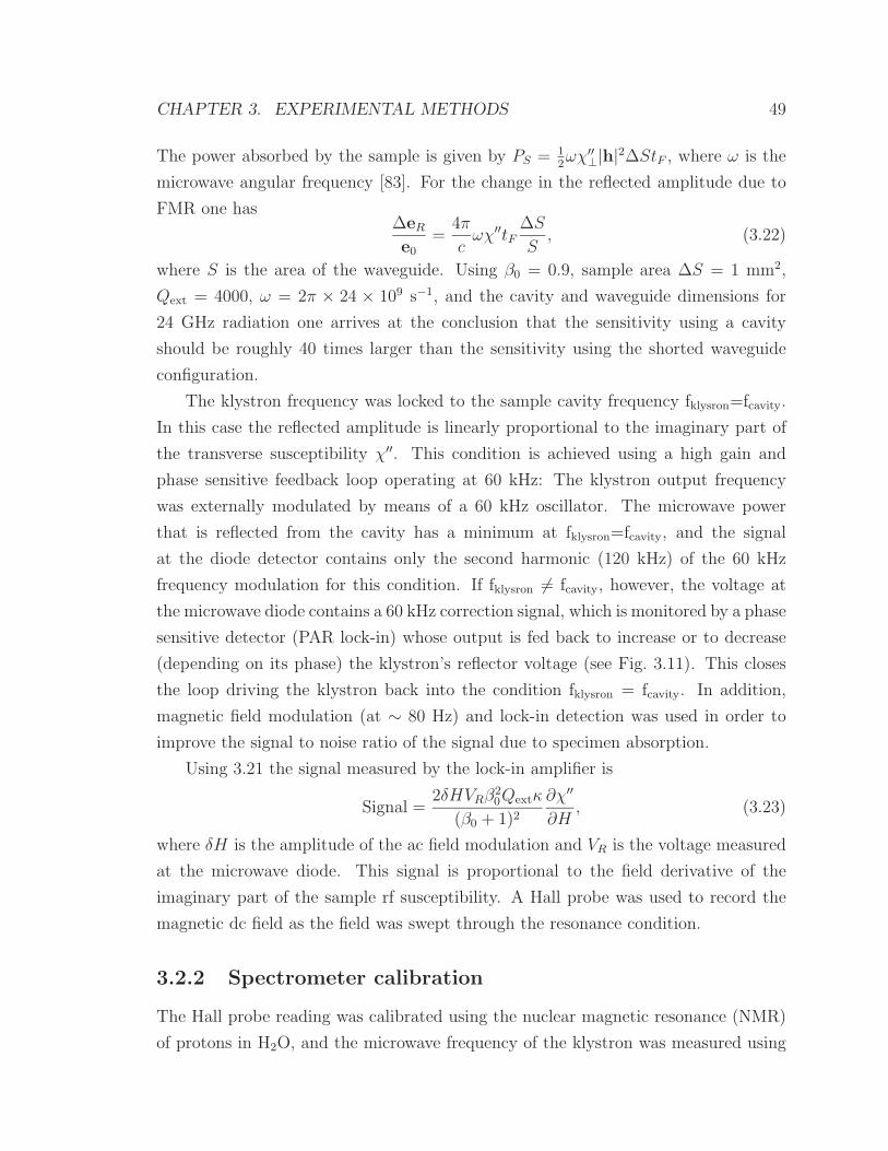
CHAPTER 3. EXPERIMENTAL METHODS 49
The power absorbed by the sample is given by PS = 12ωχ′′
⊥|h|2∆StF , where ω is the
microwave angular frequency [83]. For the change in the reflected amplitude due to
FMR one has∆eR
e0
=4π
cωχ′′tF
∆S
S, (3.22)
where S is the area of the waveguide. Using β0 = 0.9, sample area ∆S = 1 mm2,
Qext = 4000, ω = 2π × 24 × 109 s−1, and the cavity and waveguide dimensions for
24 GHz radiation one arrives at the conclusion that the sensitivity using a cavity
should be roughly 40 times larger than the sensitivity using the shorted waveguide
configuration.
The klystron frequency was locked to the sample cavity frequency fklysron=fcavity.
In this case the reflected amplitude is linearly proportional to the imaginary part of
the transverse susceptibility χ′′. This condition is achieved using a high gain and
phase sensitive feedback loop operating at 60 kHz: The klystron output frequency
was externally modulated by means of a 60 kHz oscillator. The microwave power
that is reflected from the cavity has a minimum at fklysron=fcavity, and the signal
at the diode detector contains only the second harmonic (120 kHz) of the 60 kHz
frequency modulation for this condition. If fklysron = fcavity, however, the voltage at
the microwave diode contains a 60 kHz correction signal, which is monitored by a phase
sensitive detector (PAR lock-in) whose output is fed back to increase or to decrease
(depending on its phase) the klystron’s reflector voltage (see Fig. 3.11). This closes
the loop driving the klystron back into the condition fklysron = fcavity. In addition,
magnetic field modulation (at ∼ 80 Hz) and lock-in detection was used in order to
improve the signal to noise ratio of the signal due to specimen absorption.
Using 3.21 the signal measured by the lock-in amplifier is
Signal =2δHVRβ2
0Qextκ
(β0 + 1)2
∂χ′′
∂H, (3.23)
where δH is the amplitude of the ac field modulation and VR is the voltage measured
at the microwave diode. This signal is proportional to the field derivative of the
imaginary part of the sample rf susceptibility. A Hall probe was used to record the
magnetic dc field as the field was swept through the resonance condition.
3.2.2 Spectrometer calibration
The Hall probe reading was calibrated using the nuclear magnetic resonance (NMR)
of protons in H2O, and the microwave frequency of the klystron was measured using

CHAPTER 3. EXPERIMENTAL METHODS 50
∆
χ
Figure 3.13: Typical FMR spectrum measured at 24 GHz using a 120Au/16Fe/GaAs
sample. The open circles show the data and the solid line is a fit to Eq. 3.25. The peak-to-
peak linewidth ∆HPP = 50 Oe and the resonance field HFMR = 4.15 kOe are indicated on
the diagram.
a calibrated cavity frequency meter. The frequency calibration was independently
checked by means of the electron spin resonance (ESR) of the electron free radical
species in diphenylpicrylhydrazyl (DPPH) characterized by g = 2.0037 [84].
3.2.3 Typical spectra
An FMR spectrum contains two important pieces of information: line position and
linewidth. The line position is given by the internal fields, and their angular and fre-
quency dependence allows one to determine magnetic anisotropies, effective magneti-
zation, and g-factor. The linewidth is related to the magnetic damping (see Eq. 2.25)
and the angular and frequency dependence of the linewidth provides information
about the magnetic damping mechanism.
The line position and linewidth were usually extracted by fitting the FMR data to
the derivative of an asymmetric Lorentzian. Asymmetry has to be considered because
the coupling between the magnetic sample and microwave cavity can partly mix real

CHAPTER 3. EXPERIMENTAL METHODS 51
and imaginary parts of the susceptibility. The asymmetric absorption function is
given by
cos εχ′′ + sin εχ′ ∼ ∆H cos ε + (H − HFMR) sin ε
∆H2 + (H − HFMR)2, (3.24)
and the function used to fit the FMR data is its derivative with respect to H
d[cos εχ′′ + sin εχ′]dH
∼ − 2(H − HFMR)∆H cos ε
[∆H2 + (H − HFMR)2]2−[∆H2 − (H − HFMR)2
]sin ε
[∆H2 + (H − HFMR)2]2, (3.25)
where ε denotes the mixing angle between dispersive and absorptive components and
∆H is the half width at half maximum (HWHM) of the absorption line. It is possible
that the cavity absorption peak is a superposition of several modes operating at the
same frequency due to perturbations introduced by the sample. When the sample
undergoes FMR only the modes with large h field at the sample position are detuned
while the feedback mechanism is sensitive to the overall absorption of the cavity
and may lock to the spurious modes. This situation would lead to an admixture of
dispersion into the absorption and cause asymmetric line shapes. Another possible
reason for asymmetric lines is the skin effect, but the magnetic films studied in this
thesis are very thin compared to the skin depth. The asymmetry was usually found
to be weak (ε = 0 − 10), as shown in Fig. 3.13.
For fairly symmetric lines the resonance field and linewidth are easy to determine.
The resonance field is given by the zero crossing, and the peak-to-peak line width
∆HPP is equal to the separation between the inflection points, see Fig. 3.13. The
peak-to-peak linewidth is related to the HWHM ∆H by
∆H =
√3
2∆HPP . (3.26)

CHAPTER 3. EXPERIMENTAL METHODS 52
3.3 Magneto-Optic Kerr Effect
The magneto-optic Kerr effect (MOKE) allows one to use light to determine the
direction of the magnetization. The polarization vector of the incoming light rotates
slightly upon reflection from a magnetic sample [57, 58], as described in section 2.6.
3.3.1 Static MOKE system
A high sensitivity MOKE system for longitudinal and transverse Kerr measurements
was built at SFU as part of this thesis. A schematic diagram of this setup is shown
in Fig. 3.14. The light source is an intensity stabilized laser diode (535 nm) with
an anamorphic prism pair that is used to transform the elliptical beam profile (from
the laser diode) into a nearly circular Gaussian beam. The magnetic sample is placed
between two Glan-Thompson polarizers (P1 and P2) and the light beam is p-polarized
(in the plane of incidence) and focussed onto the sample. The diameter of the focussed
beam spot on the sample is ∼ 100 µm. The optical direction of the analyzer is oriented
almost perpendicular to the plane of incidence. Behind the analyzer, P2, the light is
focussed onto a high-gain low-noise Si hybrid detector. An interference filter (IF) with
its center wavelength matched to the laser diode (535 nm) is placed in front of the
detector to suppress ambient light. The sample is mounted on a X-Y-θ-φ stage which
is installed on a motorized rotational drive. The translation allowed one to adjust
the sample position while the tilt is used to adjust the plane of the sample to be
perpendicular to the rotational axis. The sample is placed between the pole pieces of
a four quadrant electromagnet which permitted fields up to 2 kOe to be oriented in an
arbitrary direction in the film plane. It is therefore possible to measure both in-plane
components of the magnetization (in longitudinal and transverse Kerr configurations)
by switching the magnetic dc field from parallel to the optical plane of incidence
to perpendicular to the optical plane. This is achieved by rotating the sample and
field by 90, but leaving the optical setup unchanged. The magnetic contrast (due to
rotation of the polarization) is optimal in this setup because no optical components
other than the sample are placed between polarizer and analyzer.
3.3.2 Time resolved MOKE microscopy
High resolution Kerr microscopes are less sensitive than the above system because
they require an objective lens to be placed between polarizer and analyzer. In order

CHAPTER 3. EXPERIMENTAL METHODS 53
Figure 3.14: Experimental setup used for longitudinal and transverse MOKE measure-
ments.
to achieve time resolution in Kerr effect imaging, two additional ingredients (compared
to static microscopy) are necessary: (i) a pulsed light source and (ii) a synchronous
means of magnetic excitation of the sample. A good review of time-resolved Kerr
microscopy (TRMOKE) can be found in [85].
Spatial resolution requires scanning of either sample or laser beam. The magne-
tization of the sample is excited by a magnetic field pulse with a rise time of a few
ps generated by an optical pulse (the pump beam). Time resolution is achieved by a
stroboscopic technique using a pump and a probe beam. After the sample is excited
(pumped) the sample is interrogated (probed) at a delay time τ using an ultrashort
light pulse to measure the time evolution of the perpendicular component of the mag-
netization (polar MOKE). The source of the ultrashort light pulses is a commercial
Titanium Sapphire (Ti:Sa) Laser system with ∼ 100 fs pulse width, a repetition rate
of ∼ 80 MHz, and a wavelength of 800 nm. A beam splitter (BS) is used to split the
light into pump (field pulse generation) and probe (Kerr effect measurement) beams,
as illustrated in Fig. 3.15. The optical path length of the pump beam is variable, so
that the probe pulses can be delayed with respect to the pump pulses (see Fig. 3.15).
Most of the 1/f noise and non-magnetic signals are suppressed by using a lock-in tech-
nique. The 80 MHz pulse train used to generate the magnetic field pulses (the pump
pulses) is modulated using an optical chopper operating at 1.5 kHz and the signal
coming from the photodiodes is fed into a lock-in amplifier sensitive to this frequency;
see Fig. 3.16 for an illustration of the pump probe pulse sequence. In this way it is
possible to use low-bandwidth and low-noise photodiodes and amplifiers. The time

CHAPTER 3. EXPERIMENTAL METHODS 54
Figure 3.15: (a) Optical layout of the TRMOKE setup used at the University of Regensburg.
A Coherent Ti:Sa laser system provides light pulses having 100 fs duration at a repetition rate
of 76 MHz. The pump beam has a wavelength of 800 nm and the probe beam is frequency
doubled (400 nm). Exciting field and external bias field are oriented in the sample plane.
(b) Optical layout of the TRMOKE setup used at the University of Alberta. A Spectra
Physics Ti:Sa laser system provides pulses having 100 fs duration at a repetition rate of
82 MHz. The pump and probe beams have a wavelength of 800 nm. The bias field is in
the sample plane and the magnetic field pulses are generated in a photo conductive switch
(PC) and are perpendicular to the plane of the sample. In both setups the delay line and
the chopper are part of the pump beam circuit. Kerr effect measurements are performed
using a Wollaston polarizer (P2) and two detectors operated in differential mode. Spatial
resolution is achieved by scanning the sample under the microscope objective lens (MO).

CHAPTER 3. EXPERIMENTAL METHODS 55
0.7 ms
12 ns
pump
probe
Figure 3.16: Pulse sequence for pump and probe beams. The 12 ns interval between
individual pulses corresponds to the 80 MHz repetition rate of the laser. Pump and probe
are delayed with respect to each other by a delay time τ and the pump pulses are chopped
at 1.5 kHz.
interval between subsequent laser pulses is 12 ns (1/80 MHz) and sufficiently long for
the magnetization to reach equilibrium after having been perturbed by a pump pulse.
Two different systems are used in this thesis for time resolved Kerr studies and
the different methods of exciting the magnetization will be discussed in the following.
Schottky barrier as field source (Regensburg)
In the TRMOKE setup at the University of Regensburg the Schottky barrier of the
Fe/GaAs interface is used to generate magnetic field pulses. When a biased Schottky
barrier between the n-doped GaAs substrate and ferromagnetic film is illuminated by
a light pulse, the resulting photo current gives rise to a circular magnetic field pulse in
the plane of the sample [86], as illustrated in Fig. 3.17a. The photons from the pump
beam (800 nm 1.54 eV) create electron-hole pairs in the semiconducting substrate
beneath the magnetic film. A photo current is generated when electrons and holes are
spatially separated by an electric field. In the absence of an externally applied bias
voltage the band curvature (built-in voltage) at the Fe/GaAsn interface separates
electrons and holes, thereby generating a photo current directed perpendicular to
the interface. This photocurrent can be enhanced by a factor of 4 by applying a
voltage to reverse bias the Schottky diode, and hence sweep out the carriers from the
depletion region faster [87]. The macroscopically measured pump current is about
20 mA [86]. Assuming a Gaussian spatial distribution for the current (corresponding
to the pump beam intensity profile) and using the rise and fall times of the current

CHAPTER 3. EXPERIMENTAL METHODS 56
pulse (determined from the time dependent reflectivity of the Schottky barrier) the
amplitude of the field pulse was estimated to be ∼ 25 Oe [87]. The current pulse rises
to its full amplitude within a few ps and the fall time was estimated to be ∼ 120 ps
without bias and less than 50 ps when applying a reverse bias voltage larger than 1
V [87].
A n+-doped GaAs(001)n+wafer (5 × 1019 cm−3 carriers) was covered with a n-
doped GaAs buffer layer (5×1017 cm−3 carriers) deposited using metal organic vapor
deposition (MOCVD). The lower doping level in the buffer layer ensured a high Schot-
tky barrier at the Fe/GaAs interface. At the same time the n+-doping of the substrate
allowed easy formation of an ohmic contact to a gold wire on the other side of the
wafer using an InGa eutectic solder [88], as shown in Fig. 3.17a. The best Schottky
diodes are obtained when the GaAs wafers are not annealed after hydrogen cleaning.
Even then the Fe/GaAs Schottky barriers were found to be leaky with ideality fac-
tors around ∼ 1.1 and barrier heights of ∼ 0.6 eV. Similarly poor characteristics of
Fe/GaAs Schottky diodes have been reported by other groups (using different prepa-
ration techniques) [89, 90, 91]. Therefore, it appears likely that Fe/GaAsn Schottky
barriers are intrinsically leaky.
In order to allow straightforward optical separation of the reflected pump and
probe beams, the probe beam is frequency doubled in a Barium Beta-Borate (BBO)
crystal and recombined with the pump beam using a dielectric mirror. Both, the
pump beam (800 nm) and the probe beam (400 nm) are then fed into a polarization
maintaining microscope (Zeiss Axiomat) and focussed by the same objective lens, as
illustrated in Fig. 3.17a. The polarization changes of the reflected probe beam are
detected using a Wollaston polarizer and diode detectors operated in a differential
mode.
Strip line as a field Source (Edmonton)
In the measurements carried out at the University of Alberta in the group of Profes-
sor Mark Freeman a microwave transmission line is used to generate the magnetic
pump field pulses. The wave guide (slot line) is connected to a reverse biased GaAs
photoconductive switch (PC). The pump beam illuminates the PC switch, and gen-
erates a current pulse which travels down the waveguide discharging the capacitance
of the biased slot line. The conductors of the waveguide are deposited on a thin glass
substrate and the gap between the conductors is tapered down to 10 µm in width in

CHAPTER 3. EXPERIMENTAL METHODS 57
M
Pump Probe
4nm Au/2nm Fe
VB
GaAs n (001)+
GaAs n
+
a Objective lens
HB
VB
GaAsPC
Sample
b
HB
Figure 3.17: (a) Exciting field generated by the Fe/GaAs Schottky diode. The pulsed
magnetic field is circular and lies in the plane of the sample. (b) Waveguide used to generate
the magnetic pump field at the University of Alberta. A GaAs based photo conductive switch
(PC) is attached to the Au waveguide by short Indium wires and the gap of the waveguide
provides optical access to the sample. The orientation of the magnetic bias field, HB, is
indicated in both configurations.
order to maximize the pump field intensity. The magnetic film side of the Fe/GaAs
sample is pressed directly onto the waveguide, and the time evolution of the mag-
netization is monitored through the (waveguide supporting) glass plate in the region
of the 10 µm wide gap of the slot line (see Fig. 3.17b). In this configuration the
pump field is mainly oriented perpendicular to the film plane. Due to the presence
of the waveguide supporting glass plate (0.5 mm thickness) between the microscope
objective lens and the magnetic film, the spatial resolution is limited to ∼ 2 µm. This
setup delivers magnetic field pulses oriented perpendicular to the film plane with an
amplitude of ∼ 20 Oe, and rise and fall times of 10 ps and 100 ps, respectively.

Chapter 4
Damping in Au/Fe/GaAs
Multilayers
In this chapter the static and dynamic properties of Au/Fe/GaAs magnetic single
layers and Au/Fe/Au/Fe/GaAs magnetic double layers will be presented. It will
be shown that the magnetic double layers are affected by an additional relaxation
mechanism that can be described by a spin-pump and spin-sink model.
4.1 Sample Growth
The preparation of the Au/Fe/GaAs(001) film structures was carried out by means of
Molecular Beam Epitaxy (MBE). Semi-insulating epi-ready GaAs(001) wafers were
used as templates for the growth of Fe. The GaAs substrates were mostly cleaned by
hydrogen cleaning (see section 3.1.1 for details) and subsequently annealed at 600 C.
The annealing process was monitored by means of Reflection High Energy Electron
Diffraction (RHEED) until a well defined (4 × 6) reconstruction appeared [67].
All metallic films were deposited at RT from thermal sources at base pressures
less than 2 × 10⁻¹⁰ torr and deposition rates of ∼ 2 ML/min. The film thicknesses
were monitored by means of a quartz crystal microbalance and RHEED intensity
oscillations.
Fe(001) has a lattice constant that is only 1.4% smaller than the size of the
half unit cell of GaAs(001) and therefore the in-plane epitaxial relation is [100]Fe ‖[100]GaAs. From the size of this mismatch one can anticipate that the critical thickness
for the formation of misfit dislocations is about 10 nm [92, 93]. RHEED oscillations
58

CHAPTER 4. DAMPING IN AU/FE/GAAS MULTILAYERS 59
Figure 4.1: RHEED intensity oscillations of (a) 30 ML Fe on GaAs(001) and (b) 20 ML
Au on 15Fe/GaAs(001).
Figure 4.2: RHEED pattern of (a) a 15Fe/GaAs(001) surface with the electron beam
oriented along the 〈110〉Fe direction and (b) a 20Au/15Fe/GaAs(001) surface with the
primary beam oriented along the 〈100〉Au direction. Note that additional streaks appear
(indicated by arrows) between the zeroth and first order diffraction streaks due to the 2× 2
reconstruction of As that behaves like a surfactant.
during the growth of Fe on GaAs(001) were visible for up to 50 ML indicating an
excellent quasi layer-by-layer growth (see Fig. 4.1a). During the initial stages of
growth the RHEED oscillations are weak, but after deposition of roughly 3 atomic
layers, a continuous film is formed [94] and the intensity of the specular spot as
well as the amplitude of the RHEED oscillations increase dramatically, as shown in
Fig. 4.1a. All of the Fe samples that were studied were thicker than 7 ML. This
avoided complexities that might be related to the initial phase of the growth. X-
ray Photoemission Spectroscopy (XPS) measurements indicated that during the Fe

CHAPTER 4. DAMPING IN AU/FE/GAAS MULTILAYERS 60
GaAs(001)
31 Fe
40 Au
40Fe
20 Au
10 nm
Figure 4.3: High resolution cross-sectional TEM image of a 20Au/40Fe/40Au/31Fe/GaAs
multilayer. The sample was tilted by 1 to enhance the contrast between the Au and Fe
layers.
deposition on GaAs, approximately 0.6 ML of As segregated on top of the Fe film [67].
After deposition of additional metallic layers the same amount of As was found on the
surface. This implies that the As atoms are floating and act as a surfactant; i.e. no
As stays inside the metallic layers or interfaces. The RHEED intensity oscillations for
Au on Fe/GaAs were visible for up to 20 atomic layers, as shown in Fig. 4.1b. Due to
the presence of As atoms at the surface the RHEED diffraction patterns of Au(001)
always showed a 2 × 2 reconstruction instead of the usual 5 × 1 reconstruction, as
illustrated in Fig. 4.2b. The lattice mismatch between Fe(001) and Au(001) is only
0.5% with 〈110〉Au ‖ 〈100〉Fe. The presence of RHEED intensity oscillations for all
layers suggests that the roughness is confined to 3 atomic layers across distances of the
order of 100 nm. This was confirmed using high resolution cross-sectional transmission
electron microscopy (XTEM). Fig. 4.3 shows an atomic resolution XTEM image of
a Au/Fe multilayer grown on GaAs(001). The thicknesses obtained by counting the
individual atomic layers from the TEM image agrees perfectly with the thicknesses

CHAPTER 4. DAMPING IN AU/FE/GAAS MULTILAYERS 61
χµ
ϕ
Figure 4.4: (a) Typical FMR spectra measured at 23.9 GHz with the applied field oriented
along the [110]Fe, [100]Fe, and [110]Fe directions on a 20Au/10Fe/GaAs(001) sample. The
low peak intensity along the [110]Fe direction is due to the fact that the rf driving field in-
side the microwave cavity was almost parallel to the [110]Fe direction and was therefore very
ineffective at exciting the magnetization since for this case M and h were almost parallel.
(b) () symbols represent the measured in-plane angular dependence of the resonance field
HFMR, where ϕH is the angle of the applied field measured with respect to the [100]Fe direc-
tion. The solid line is the theoretical dependence which was calculated using the following
magnetic parameters as fitting coefficients: K1 = 1.8 erg/cm3, KU = −8.4 erg/cm3, and
4πMeff = 16.5 kOe (the g factor was fixed at g = 2.09 for this fit).
determined from the RHEED intensity oscillations observed during the film growth.
As expected from the small lattice mismatch, very few dislocations are observed in
XTEM, with an average separation of approximately 80 nm.
4.2 Magnetic Properties of Au/Fe Single Layers
FMR and MOKE were used to determine the magnetic properties of the Fe layers
directly grown on the GaAs. A series of 4 magnetic single layer samples was prepared:
20Au/nFe/GaAs(001), where the integers represent the number of atomic layers and
n was 8, 11, 16, and 31 ML. The FMR absorption peaks were narrow and symmetric
Loretzian lines, as illustrated in Fig. 4.4a.

CHAPTER 4. DAMPING IN AU/FE/GAAS MULTILAYERS 62
Film K||,B1 [105 erg
cm3 ] K||,S1 [10−2 erg
cm2 ] K||,SU [10−2 erg
cm2 ] 4πMS [kG] K⊥,SU [10−2 erg
cm2 ]
AuFeGaAs 4.3 ± 0.1 −3.5 ± 0.3 −14 ± 1 20.8 ± 0.2 88 ± 4
AuFeAu 4.6 ± 0.3 −4.5 ± 0.3 20.5 ± 0.3 90 ± 10
Table 4.1: Values of the interface (S) and bulk (B) contributions to the magnetic
anisotropies determined from the data shown in Fig. 4.5. The interface anisotropies corre-
spond to the sum of the contributions from both interfaces.
Magnetic Anisotropies
The angular dependence of the FMR field was used to determine the magnetic ani-
sotropies, effective demagnetizing field 4πMeff , and g-factor, as shown in Fig. 4.4b.
It was possible to determine 4πMeff and g by fitting self-consistently data obtained
on the same sample at different microwave frequencies. The g-factor was found to
be g = 2.09 ± 0.01, while the anisotropy values for all samples having different Fe
thicknesses tFe are shown in Fig. 4.5a. In ultrathin films the interface contribution to
the anisotropies is shared by all layers and consequently the effective anisotropies scale
inversely with the film thickness tFe (see Eq. 2.3). This behavior is clearly observed
in Fig. 4.5a where the effective anisotropies are plotted as a function of 1/tFe. The
intercept with the y-axis corresponds to infinite thickness, and therefore represents the
bulk anisotropy. The slope is related to the interface contribution of the anisotropy
(see Fig. 4.5a and Tab. 4.1). The saturation magnetization can be obtained from
the effective demagnetizing field for infinite thickness (bulk), i.e. 4πMeff = 4πMS =
20.6 ± 0.3 kOe. This leads to MS = 1640 ± 25 emu/cm3, which is very close to the
bulk value expected for Fe (see Tab. 2.1).
The values for the in-plane anisotropies reported in Tab. 4.1 are in good agreement
with results obtained by other groups [70, 95]. Brockmann et al. used a slightly
different substrate preparation technique (sputtering at elevated temperatures); their
value for K||,Fe/GaAsU was 15% smaller, while their value for K
||,Fe/GaAs1 was 20% larger
than the the value shown in Tab. 4.1 [95]. The perceived value of 4πMS can be
affected by the tetragonal distortion of the film. Gordon et al. carried out X-ray
absorption fine structure (XSAFS) measurements on Fe/GaAs(001), and showed that
a 10 ML Fe film has a c/a ratio of 1.03±0.02 [96]. Due to the magneto-elastic coupling
this tetragonal strain results in an additional bulk-like anisotropy field perpendicular
to the film surface. This strain anisotropy contributes to the effective demagnetizing

CHAPTER 4. DAMPING IN AU/FE/GAAS MULTILAYERS 63
Figure 4.5: These plots show (a) the inverse thickness dependence of the in-plane
anisotropies and effective demagnetizing field for Au/Fe/GaAs layers and (b) for the top
Fe layer in Au /Fe/Au/Fe/GaAs structures. In (b) the presence of a bulk-like uniaxial
anisotropy is very likely strain induced [70] with an easy axis parallel to the [110]Fe direc-
tion.
field [97]
4πMeff = 4πMS − 2K⊥,sU
MStFe
− 2B1(e⊥ − e‖)MS
, (4.1)
where e‖ and e⊥ are the in-plane and perpendicular strain fields and B1 is the first
magneto-elastic coupling coefficient. For Fe B1 = −2.95×10⁷ erg/cm3 [97]. Recently,
Thomas et al. [70] used high resolution x-ray diffraction to show that the strain in
Fe films on GaAs remains constant for Fe thicknesses of up to 8 nm. The values for
e‖ and e⊥ from [96] result in 2B1(e⊥ − e‖)/MS = 1.1 ± 0.5 kOe and would lower the
value for 4πMS in Tab. 4.1 slightly. Considering the fact, however, that the value for
4πMS in Tab. 4.1 is already close to the value expected for bulk iron, and given the
size of the error bar on the c/a ratio from EXAFS measurements, it is likely that the
strain anisotropy contribution is small.
Magneto-optic Kerr effect (MOKE) measurements showed that for samples with

CHAPTER 4. DAMPING IN AU/FE/GAAS MULTILAYERS 64
Figure 4.6: Static MOKE loops measured on a 20Au/15Fe/GaAs(001) sample with the
magnetic field applied along the [110]Fe, [100]Fe, and [110]Fe directions. Note that the hard
axis loop (H ‖ [110]Fe) is not linear due to presence of K‖1 in addition to K
‖U .
ϕ ϕ
Figure 4.7: HFMR as a function of the in-plane angle of the magnetic field, ϕH , for
20Au/15Fe/GaAs(001) measured at (a) 10.0 GHz and (b) 23.9 GHz.
Fe films thinner than 35 ML the [110]Fe direction is the easy magnetic axis and the
[110]Fe direction is the hard magnetic axis (see Fig. 4.6). This behavior can be easily
understood from the in-plane angular dependence of the magnetic energy without an

CHAPTER 4. DAMPING IN AU/FE/GAAS MULTILAYERS 65
applied field
E(ϕM) = K‖1 sin2 ϕM cos2 ϕM − K
‖U cos2(ϕM − ϕU), (4.2)
where ϕU = −45. The minimum energy corresponds to ϕM = 45, i.e. M ‖ [110]Fe,
and the maximum energy corresponds to ϕM = −45 (i.e. M ‖ [110]Fe), provided
that KU ≥ K1. It is interesting to note that the smallest FMR field is measured with
H applied along the 〈100〉Fe direction (see Fig. 4.7) and does not coincide with the
easy magnetic direction. The easy magnetic axis is determined by the global energy
minimum, while the angular dependence of the FMR field corresponds to a constant
stiffness (frequency) contour as a function of the applied field and field angle (see
Fig. 4.8). If only one in-plane anisotropy is present (uniaxial or four-fold), then the
FMR field minimum always coincides with the easy magnetic axis. The presence of
K1 and KU with ϕU = −45 also gives rise to 3 FMR peaks at low frequencies, as
shown in Figs. 4.7 and 4.8.
Magnetic Relaxation
The linewidths of the FMR peaks were found to be very narrow and to scale linearly
with the microwave frequency in parallel and perpendicular configurations with no
appreciable zero frequency offset, as shown in Fig. 4.9a. These features are charac-
teristic of Gilbert damping. α was determined from the slope of the linewidth as
a function of the microwave frequency. The damping parameter was found to be
α = 4.4 ± 0.3 × 10⁻³ and nearly independent of the film thickness and the orienta-
tion of the magnetization. This value is about double the intrinsic Fe bulk value (see
Tab. 2.1). The enhanced damping is probably due to the modified electronic structure
of the ultrathin film compared to the bulk in combination with impurity and interface
scattering. Recently, Safonov and Bertram have shown that electron-magnon scat-
tering caused by local perturbations in the spin-orbit interaction due to defects can
result in an additional Gilbert damping [98].
Temperature dependence of anisotropies and relaxation
In the temperature range between RT and -200 C the Gilbert damping was ob-
served to be constant, and below -200 C the linewidth increased rapidly, as shown in
Fig. 4.9b. A similar behavior was observed in Ni bulk samples (see section 2.4.3) and
can be explained by increased electron mean free path at low temperatures.

CHAPTER 4. DAMPING IN AU/FE/GAAS MULTILAYERS 66
ϕFigure 4.8: Calculated contour plot of resonance frequencies versus the in-plane applied
field angle and field strength for the 20Au/16Fe/GaAs sample. White corresponds to f ≥ 18
GHz and black is equivalent to f = 0 GHz. The black lines highlight the 18, 14, and 10
GHz contours. Note that the 10 GHz contour is not continuous and splits into an ellipse
and a line around the hard axis giving rise to 3 separate FMR fields between 8 and 10 GHz,
as observed in Fig. 4.7. This is further illustrated in the inset, where calculated resonance
frequency as a function of bias field along the hard direction ([110]Fe) with a misalignment
of 0.2 (to break the symmetry) is shown.
Uniaxial and four-fold in-plane anisotropies exhibit a strictly linear temperature
dependence in the range between RT and -200 C and increase with decreasing tem-
perature, as shown in Fig. 4.10.

CHAPTER 4. DAMPING IN AU/FE/GAAS MULTILAYERS 67
Figure 4.9: (a) Frequency dependence of the FMR linewidth for the 20Au/16Fe/GaAs
sample. The magnetic field was applied along the [100]Fe direction. (b) Temperature
dependence of the FMR linewidth measured with the same sample at 10 GHz as a function
of temperature. The magnetic field was applied along the [110]Fe direction.
Figure 4.10: Temperature dependence of the in-plane anisotropies measured with a
20Au/18Fe/GaAs sample at 24 GHz (a) K‖1 and (b) K
‖U .
4.3 Magnetic Double Layers
The intrinsic relaxation properties obtained for Au/Fe/GaAs single layer films en-
able one to test the influence of a second ferromagnetic layer on magnetic relaxation.
Magnetic multilayers are a special case where the interaction between itinerant elec-
trons and magnetic moments can lead to unprecedented and exciting effects in spin
dynamics. The electric resistance of a magnetic double layer depends on the rela-
tive orientation of the magnetic moment of the two layers; this effect is called Giant

CHAPTER 4. DAMPING IN AU/FE/GAAS MULTILAYERS 68
Magneto-Resistance (GMR). Berger [99, 100, 101] and Slonczewki [102, 103] pointed
out that the inverse process can also take place. That is, the direction of the current
flowing perpendicular to the interfaces can change the relative orientation of magnetic
moments in magnetic double layers (parallel or antiparallel). Recently, this switching
effect has been experimentally realized in point contacts [104, 105] and nano-pillars
[106, 107]. Slonczewski [102] has shown that the flow of spin momentum that is carried
by a current flowing perpendicular to the interfaces of a magnetic double layer system
NM/F1/NM/F2/NM results in Landau Lifschitz like torques (see Eq. 2.5) acting on
layers F1 and F2 and the sense of this torque depends on the direction of the current.
Here NM stands for normal metal and F1,2 stand for a ferromagnetic metal. The
magnetization in F2 is usually assumed to be fixed, while the magnetization in F1
is allowed to precess (free magnetic layer). Very high current densities lead to spin
torques that can overcome the intrinsic damping torques and lead to spin instabilities
and switching phenomena [103]. Spin instabilities in turn can lead to phase coherent
emission of microwaves in the presence of a magnetic field. This phenomenon was
recently observed by the Cornell and NIST groups [108, 109].
4.3.1 Berger’s model
Berger’s treatment of a current flowing perpendicular to the NM/F1/NM/F2/NM
layer system differs from Slonczewski’s approach: the magnetization in layer (F2) is
assumed to be static and precession of the magnetization of the free layer F1 is ex-
plicitly included using a magnon occupation number. The itinerant electrons entering
F1 cannot immediately assume the instantaneous direction of the precessing magne-
tization. This leads to an exchange torque directed towards the equilibrium axis and
corresponds to an additional relaxation torque acting on the F1/NM interface. This
torque is shared by the whole magnetic film due to exchange coupling. Conserva-
tion of the total angular momentum requires that spins in the normal metal layer be
flipped. An electron spin in the NM layer has to flip from up to down as a magnon
in FM is annihilated and vice versa. The rate equations for spin up and spin down
electrons can be derived from Fermi’s golden rule which includes the interaction with
magnons [99]. This leads to a shift of the Fermi levels for spin up and spin down
electrons ∆µ = ∆µ↑−∆µ↓, and causes an additional relaxation torque which may be
written as [99, 110]
HBerger ∼ (∆µ + ω)m1 × m2, (4.3)

CHAPTER 4. DAMPING IN AU/FE/GAAS MULTILAYERS 69
where m1,2 are the unit vectors of the magnetizations in layers F1 and F2. The
absolute value and sign of ∆µ are determined by the density and direction of the
current flowing perpendicular to the interfaces. Note that the second term in Eq. 4.3
is proportional to the microwave frequency and is always positive. This term is not
present in Slonczewski’s model because it does not include the dynamic s-d interaction.
This term is present even in the absence of a current flowing though the interfaces
and represents an additional Bloch-Blombergen like interface damping [83].
4.3.2 Experimental test
Berger’s predictions regarding additional interface damping can be tested by com-
paring the magnetic damping in the Au/Fe/GaAs single layer structures discussed in
the previous section with the magnetic damping observed in magnetic double layer
Au/Fe/Au/Fe/GaAs structures. The absence of extrinsic damping in the magnetic
single layer samples allows one to isolate the effect of the second magnetic layer (F2)
on the damping in the first magnetic layer F1. A series of double layer samples
complementary to the single layer samples was grown: 20Au/40Fe/40Au/nFe/GaAs,
where n was 8, 11, 16, 21, and 31. The Au spacer thickness was chosen such that the
interlayer exchange coupling was very small but electron transport across the spacer
remained ballistic. The electron mean free path in Au grown on an Fe/GaAs(001)
template was found to be 38 nm, i.e. ∼ 190 ML Au [111]. The spin diffusion length
in Au is much bigger than the electron mean free path and was estimated by Johnson
to be lAusd ≈ 1 µm [112]. Therefore spin transport between the ferromagnetic layers
F1 and F2 through the 8 nm thick Au spacer is unimpeded by electron scattering.
Fig. 4.12a shows a typical FMR spectrum acquired from a double layer sample at 36.6
GHz. The two absorption peaks corresponding to the two layers (F1 and F2) are well
separated (by ∼ 1 kOe) because the bottom and the top layer have different interface
anisotropies and thicknesses. This allows one to measure a FMR spectrum of layer F1
while layer F2 is detuned from resonance and has a negligible precessional angle, and
vice versa. The FMR linewidth in single and double layers was also observed to be
only weakly dependent on the angle of the static magnetization (see Fig. 4.11b). The
good agreement between the FMR fields of the magnetic single layer and the bottom
layer in the corresponding double layer (see Fig. 4.11a) shows that the interlayer ex-
change coupling is negligible (j1 ≤ 0.03 erg/cm3) and that the magnetic properties of
the Au/Fe/GaAs film system are very reproducible.

CHAPTER 4. DAMPING IN AU/FE/GAAS MULTILAYERS 70
ϕ
∆
ϕ
Figure 4.11: Angular dependence of (a) FMR field and (b) FMR linewidth in the
20Au/40Fe/40Au/10Fe/GaAs double layer and 20Au/10Fe/GaAs single layer structure
measured at 36.6 GHz. () symbols represent the data for the 10Fe single layer and (•)symbols represent the 10Fe bottom layer in the double layer sample. The solid line in (a)
corresponds to the resonance field of the 40Fe top layer in the double layer structure.
χµ
∆
Figure 4.12: (a) FMR spectrum of the magnetic double layer 20Au/40Fe/40Au/11Fe/GaAs
at 36.6 GHz with M ‖ [100]Fe. The dashed line shows the FMR signal measured on the
corresponding single layer sample 20/11Fe/GaAs(001). Note that the amplitude of the
dashed line is ∼ 30% bigger than expected from the ratio of the linewidths; this was caused
by the different size of the samples. (b) Frequency dependence of ∆H for 16Fe in the
20Au/16Fe/GaAs () single layer and 20Au/40Fe/40Au/16Fe/GaAs (•) double layer with
M ‖ [100]Fe. The () symbols correspond to the difference of single and double layer
linewidths and the dotted line shows the frequency dependence of the additional linewidth
as predicted by Berger’s theory scaled to fit the experimental data.
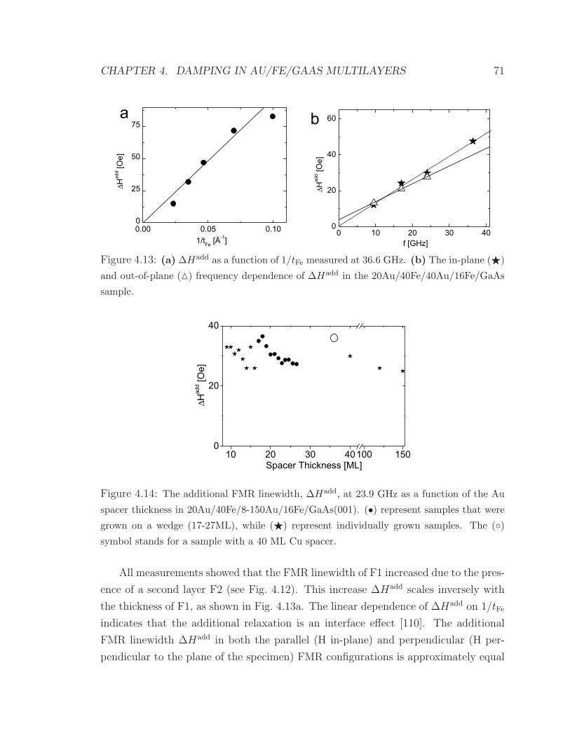
CHAPTER 4. DAMPING IN AU/FE/GAAS MULTILAYERS 71
∆ ∆
Figure 4.13: (a) ∆Hadd as a function of 1/tFe measured at 36.6 GHz. (b) The in-plane ()
and out-of-plane () frequency dependence of ∆Hadd in the 20Au/40Fe/40Au/16Fe/GaAs
sample.
∆
Figure 4.14: The additional FMR linewidth, ∆Hadd, at 23.9 GHz as a function of the Au
spacer thickness in 20Au/40Fe/8-150Au/16Fe/GaAs(001). (•) represent samples that were
grown on a wedge (17-27ML), while () represent individually grown samples. The ()symbol stands for a sample with a 40 ML Cu spacer.
All measurements showed that the FMR linewidth of F1 increased due to the pres-
ence of a second layer F2 (see Fig. 4.12). This increase ∆Hadd scales inversely with
the thickness of F1, as shown in Fig. 4.13a. The linear dependence of ∆Hadd on 1/tFe
indicates that the additional relaxation is an interface effect [110]. The additional
FMR linewidth ∆Hadd in both the parallel (H in-plane) and perpendicular (H per-
pendicular to the plane of the specimen) FMR configurations is approximately equal

CHAPTER 4. DAMPING IN AU/FE/GAAS MULTILAYERS 72
in magnitude, linearly dependent on the microwave frequency, and has no appreciable
zero frequency offset [13] (see Fig. 4.13b). For all double layers the additional Gilbert
damping is found to be only very weakly dependent on the crystallographic direction.
For the 10ML Fe film the average value is αadd10Fe = 11.0 ± 0.5 × 10⁻³. This is almost
triple the intrinsic Gilbert damping in the single Fe films, αint = 4.4± 0.3× 10⁻³ (see
Fig. 4.11b).
Berger’s theory predicts that the strength of the additional damping depends
on the average spin-flip relaxation time, conduction electron densities, and volume
fractions of F1, F2, and NM (see Eq. (19) in [99] and Eq. (10) in [101]). As a
consequence, the additional damping becomes a function of the respective volume
fractions of F1, F2, and NM. For very thin Au spacers (20-30 ML) his predicted value
for the additional damping strength is roughly double the experimentally observed
value. Moreover, experimentally the additional damping is independent of the spacer
thickness for Au spacers having thicknesses ranging from 12 to 150 ML (while keeping
the thicknesses of F1 and F2 fixed), as can be seen in Fig. 4.14. In Berger’s theory the
magnitude of the additional damping depends on the ellipticity of the precession of the
magnetization. This corresponds to a strange type of ‘Bloch-Blombergen’ damping
with a frequency dependent relaxation parameter, as shown by the dotted line in
Fig. 4.12b. This aspect of Berger’s model is in disagreement with the experimental
results, only simple Gilbert damping was observed.
4.4 Spin-Pump/Spin-Sink Theory
Brataas et al. [113] have generalized the theory of peristaltic charge pumping [114] by
including a spin dependent scattering potential. Peristaltic charge pumping is based
on the quantum mechanical scattering matrix approach introduced by Landauer and
Buttiker [115]. Tserkovnyak et al. [116] showed that an interface Gilbert damping
can be created by spin current flowing away from a ferromagnet (F) into adjacent
normal metal reservoirs (NM). A complete derivation of the spin-pumping theory is
given in appendix C. The emission of spin current is a consequence of the precessing
magnetization. Scattering at the time dependent spin potential at the F/NM interface
leads to a ‘peristaltic’ spin-pumping. The flow of the spin current is perpendicular
to the F/NM interface, and oriented from F into NM. The direction of the spin
CHAPTER 4. DAMPING IN AU/FE/GAAS MULTILAYERS 73
momentum carried away by this current is given by [116]
jspin =
4πArm × dm
dt, (4.4)
where m is the unit vector of the magnetization in F and Ar is an interface scattering
parameter. Note that the spin current is a tensorial quantity where each component
is a vector. Ar is given by
Ar =1
2
∑m,n
|r↑mn − r↓mn|2 + |t↑mn − t↓mn|2
, (4.5)
where r↑↓mn and t↑↓mn are the electron reflection and transmission matrix elements at the
NM/F interface for the spin up and spin down electrons of the transverse modes n,m
at the Fermi level. Spin-pumping theory is an adiabatic concept, i.e. the electrons
inside the NM spacer are always in equilibrium with the precessing magnetization
at the NM/F interface. To illustrate this one can compare the time an electron
spends in the NM spacer before it scatters at the NM/F interface with the time of a
precessional period of the ferromagnet. At 10 GHz and for a 10 nm thick NM spacer
the precessional period is 10−10 s while the spacer transit time is only τ = tNM/vF ∼10−14 s. Therefore the adiabatic approximation is clearly valid.
Brataas et al. [113, 117] further showed that Ar can be evaluated from the interface
spin mixing conductance G↑↓ [118]. Ar = he2 G
↑↓ = Sg↑↓, where g↑↓ represents the
dimensionless interface spin mixing conductivity. For interfaces with some degree of
diffuse scattering, g↑↓ is very close to the number of the transverse channels in the
NM and is given by [117]
g↑↓ =k2
F
4π=
32/3
4π1/3n2/3 , (4.6)
where S is the area of the interface, kF is the Fermi vector in NM, and n is the density
of electrons per spin in the NM.
Once the spin current is generated, it traverses through the normal metal spacer,
and is deposited at the NM/F2 interface. Zangwill et al. [119] recently showed that the
transverse component of the spin current is entirely absorbed at the NM/F2 interface.
For small precessional angles and assuming that M1 ‖ M2 the spin current is almost
entirely transverse with respect to the direction of the static magnetization. This
means that the NM/F2 interface acts as an ideal spin-sink, and therefore provides a
spin brake for the precessing magnetic moment in F1 [13, 120, 121]. The spin current

CHAPTER 4. DAMPING IN AU/FE/GAAS MULTILAYERS 74
jspin which takes spin momentum away from F1 has the form of Gilbert damping
(compare Eqs. 4.4 and 2.8). The strength of the Gilbert damping can be evaluated
from conservation of the total angular momentum
jspin − 1
γ
∂Mtot
∂t= 0 , (4.7)
where Mtot is the total magnetic moment in F1. After simple algebraical steps (see
section C.10 for details), one obtains an expression for the dimensionless spin-pump
contribution to the Gilbert damping constant in ultrathin films,
αsp = gµBg↑↓
4πMs
1
t1, (4.8)
where t1 is the thickness of F1 and µB is the Bohr magneton. The inverse dependence
of αsp on the film thickness clearly testifies to its interfacial origin. Self-consistent
calculations using the full LLG equations of motion including the exchange interac-
tion torque have shown that the 1/t1 scaling of the damping due to spin-pumping
is almost perfectly satisfied even if the magnetic film thickness significantly exceeds
the exchange length [122]. Both layers, F1 and F2, act as mutual spin-pumps and
spin-sinks. For small precessional angles the equation of motion for F1 can be written
as [121]
∂m1
∂t= − γ
[m1 × H1
eff
]+ α1
[m1 × ∂m1
∂t
]
+gµBg↑↓
4πMst1m1 × ∂m1
∂t− gµBg↑↓
4πMSt1m2 × ∂m2
∂t, (4.9)
where m1,2 are the unit vectors along the magnetization directions in F1 and F2,
and t1 is the thickness of F1. The exchange of spin currents is a symmetric concept
and the equation of motion for layer F2 can be obtained by the interchange of the
indices 1 2 in Eq. 4.9. The third and fourth terms on the right hand side of
Eq. 4.9 represent the spin-pump and spin-sink effects on the magnetization in F1.
The fourth term is generated by the precession (spin-pump) of the magnetization in
F2. For clarity, it is worthwhile to point out that the signs (+) and (−) in the third
and fourth terms in Eq. 4.9 represent the spin current directions (F1 → F2) and
(F2 → F1), respectively.

CHAPTER 4. DAMPING IN AU/FE/GAAS MULTILAYERS 75
4.5 Other Models for Non-Local Gilbert Damping
4.5.1 Dynamic Exchange Coupling
Since the spin-pump model is a rather exotic concept for those working in magnetism,
one would expect that there is a direct relation to a more common concept applicable
to magnetic multilayers. The obvious choice is to describe these effects as a conse-
quence of interlayer exchange coupling which has been studied extensively by a large
group of people. Historically the interlayer exchange interaction has been treated only
in the static limit [123]. Recently, this coupling has been studied for a time dependent
magnetization. It has been found that the out-of-phase part of the exchange coupling
results in magnetic damping [120, 121, 124, 125, 126]. It also has been shown that the
spin-pumping theory is equivalent to a dynamic interlayer exchange coupling [124].
Simanek and Heinrich have shown that the additional Gilbert damping is enhanced by
the square of the Stoner factor [124] when compared to the spin-pumping theory. This
calculation was based on the electron-electron interaction in an unpolarized electron
gas. In a subsequent paper Simanek considered the more realistic situation were the
electron gas is polarized by the static component of the magnetization and concluded
that the Stoner enhancement of the damping is only a small effect [125].
4.5.2 Breathing Fermi surface
The damping of magnetic double layers can be affected by the finite momentum
life time of electrons in the NM spacer. Interlayer exchange coupling is based on
the itinerant nature of the electrons. In a ferromagnet the energy of the electrons
depends on the instantaneous orientation of the magnetic moments, and consequently
the occupation number nk,σ of electronic states having energy εk,σ changes during the
precession of the magnetization, resulting in a ‘breathing Fermi surface’. This concept
was used in ferromagnetic bulk materials, as outlined in section 2.4.3; here it is applied
to the NM spacer. The redistribution of electrons cannot be achieved instantaneously
and the time lag between the instantaneous exchange field and the induced moment
in the spacer layer can be described by the transverse spin relaxation time, τsf , which
is proportional to the momentum relaxation time entering the conductivity [19]. In
the limit of slow precessional motion the effective damping field on the magnetization

CHAPTER 4. DAMPING IN AU/FE/GAAS MULTILAYERS 76
due to spin relaxation in the NM spacer can be evaluated as [120, 121],
Hdamp = τsf
∑k,σ
δ(εk,σ [M1] − εF )(
∂εk,σ [M1]∂M1
)2 1tF
∂M1
∂t, (4.10)
where the sum is carried out per unit area. In this case, the damping field is pro-
portional to the spin relaxation time τsf . This mechanism is therefore dependent on
the conductivity and represents an additional contribution to the non-local damping.
Note that the spin-pumping mechanism described in section 4.4 is independent of τsf .
4.6 Applicability of the Models
The spin-pumping and breathing Fermi surface theories predict strictly Gilbert damp-
ing. This feature was observed experimentally over a wide range of microwave fre-
quencies [121, 127], as illustrated in Figs. 4.12b and 4.13b.
The validity of the spin-pumping theory can be tested by comparing calculations
using Eqs. 4.9 with the experimental results. Fig. 4.15 shows two extreme situations.
In the left panel of Fig. 4.15 the FMR fields of F1 and F2 are separated by a big margin,
while in the right panel of Fig. 4.15 the FMR fields are the same. In the left situation
one expects the full spin-pump contribution to the damping, and ∆Hadd for layers
F1 and F2 should scale inversely with their respective thicknesses. In the right panel
the situation is symmetric; the net spin momentum current through both interfaces is
zero, and the additional damping should disappear. This behavior was experimentally
verified by measuring FMR spectra near the crossover of the FMR fields at 24 GHz,
as shown in Fig. 4.16. Asymmetry of the resonance peaks (due to an admixture of χ′
in χ′′) was avoided by placing the sample at the end of a shorted waveguide instead
of a resonant cavity for the FMR measurements. This way it was possible to analyze
the superimposed FMR spectra corresponding to F1 and F2 without the asymmetry
parameter ε described in section 3.2.3 (χ′ corrections), thereby reducing the number
of fitting parameters. Fig. 4.17 shows an example of such FMR data. The behavior
from the spin-pump spin-sink theory was obtained by calculating FMR peaks using
Eq. 4.9 and the magnetic parameters determined from FMR measurements. The
excellent agreement between the experimental results and the spin-pumping theory
is obvious in Fig. 4.17. In Fig. 4.16 the experimental and calculated spectra where
analyzed using Loretzian line shapes. The experimentally observed disappearance
of the additional damping around the crossing of the FMR fields of F1 and F2 is

CHAPTER 4. DAMPING IN AU/FE/GAAS MULTILAYERS 77
F1F2NM
effH2effH
1H
F1F2NM
effH2effH
1
DC
RFh
Figure 4.15: A cartoon of the dynamic coupling phenomenon. In the left drawing, layer
F1 is at resonance and its precessing magnetic moment pumps spin current into the spacer,
while F2 is detuned from resonance. In the right drawing, both films resonate at the same
effective field, inducing spin currents of equal amplitude in opposing directions. The short
arrows in NM indicate the instantaneous direction of the spin angular momentum ∝ mi× dmidt
carried away by the spin currents. The thin layers at the Fi/NM interfaces represent the
regions where the spin current is absorbed.
extremely well described by the theory, as illustrated in Figs. 4.16b and 4.17. The
excellent agreement between theory and experiment demonstrates the validity of the
spin-pump and spin-sink concept which is described by Eq. 4.9. It follows that even in
absence of static interlayer exchange coupling, the magnetic layers are coupled by the
dynamic part of the interlayer exchange. The spin-sink effect at the NM/F interface
starts to be inefficient only when the thickness of the NM spacer becomes comparable
to the spin diffusion length [128]. In this case spin accumulation inside the NM layer
acts as a resistance for the spin current in series with 1/g↑↓ and drives a back-flow of
spins into F [129]. In the spin-pump spin-sink model it is expected that the additional
damping is nearly independent of the Au spacer thickness considering the fact that
the spin diffusion length in Au is of the order of 1 µm [112]. This was experimentally
confirmed for thicknesses ranging from 2 to 30 nm (see Fig. 4.14). The static interlayer
exchange coupling vanishes for Au thicknesses exceeding a mere 10 ML (2 nm). This
rapid decay is caused by the Au/Fe interface roughness. One should point out that
when the NM spacer thickness becomes comparable to the spin diffusion length, then
the NM spacer can absorb a part of the spin current on its own [122, 130].
The quantitative comparison of the measured magnitude of the additional damp-
ing with the prediction from the spin-pumping theory is very favorable. First princi-
ples electron band calculations resulted in g↑↓ ≈ 1.42 × 1015 cm−2 for a Cu/Co(111)

CHAPTER 4. DAMPING IN AU/FE/GAAS MULTILAYERS 78
ϕ
∆
ϕ
Figure 4.16: (a) The FMR fields for the layer F1(16Fe, shown by ()) and the layer F2(40Fe,
()) in the 20Au/40Fe/16Au/16Fe/GaAs(001) structure at 23.9 GHz as a function of the
angle ϕH . The in-plane uniaxial anisotropy field in F1 leads to an accidental crossover at
ϕH =20 and 55. Notice that the FMR fields of F1 and F2 get locked together by the
spin-pumping effect at the accidental crossover. (b) FMR linewidths of F1()) and F2())
around the crossover at ϕH = 20. The black line was obtained from calculations using the
spin-pumping theory with the appropriate anisotropies from Fig. 4.5, the intrinsic relaxation
parameters α40Feint = 3.68 × 10⁻³, α16Fe
int = 4.0 × 10⁻³, and the spin-pumping coefficientgµBg↑↓4πMS
= 8.52 × 10⁻¹⁰ cm−1. Measured and calculated FMR spectra were analyzed using
two Lorenzian lineshapes.
interface with 2 ML of alloying [118]. By scaling this value to Au by changing n in
Eq. 4.6 and using (kCuF /kAu
F )2 = 1.26 [69] one obtains αsp16Fe = 4.4 × 10⁻³ for a 16 ML
thick Fe film. This calculated additional contribution to the damping parameter agrees
with the observed additional contribution to within 20% (αadd16Fe = 3.7 ± 0.2 × 10⁻³
measured at RT). Moreover, the additional damping observed for a sample with a Cu
spacer is 20% bigger than the values obtained for Au spacers, as shown in Fig. 4.14.
This is exactly what is expected considering that Cu has a higher density of con-
duction electrons than Au; i.e. based on the electron densities this enhancement, see
Eq. 4.6, is expected to be 26%.
This qualitative and quantitative agreement between theory and experiment is
striking. Calculations of the intrinsic damping in bulk metals have been carried
out over the last three decades; none have produced a comparable agreement with
experiments [131]. The reason is that the spin-pumping effect is calculated based
on the free electron behavior in the NM; in contrast to this the intrinsic damping

CHAPTER 4. DAMPING IN AU/FE/GAAS MULTILAYERS 79
ϕϕϕχ
µ
Figure 4.17: FMR spectra measured at 23.9 GHz around the crossover of FMR fields
in the 20Au/40Fe/16Au/16Fe/GaAs(001) structure. The spectra where measured with
ϕH = 18.5, ϕH = 22.0 (crossover), and ϕH = 29.5 (from left to right). The (•) symbols
represent the measured data and the grey solid line was calculated using Eq. 4.9 with
the anisotropies from Fig. 4.5, the intrinsic relaxation parameters α40Feint = 3.68 × 10⁻³,
α16Feint = 4.0 × 10⁻³, and the spin-pumping coefficient gµBg↑↓
4πMS= 8.52 × 10⁻¹⁰ cm−1. In all
three graphs the same scaling factor between theory and calculation was used, and individual
fine tuning of the uniaxial anisotropy field (up to 20 Oe) and angle ϕH (up to 0.5) was
allowed to obtain a perfect agreement between theory and experiment.
in metallic ferromagnets depends on difficult relativistic and spin dependent electron
band properties, as outlined in section 2.4.3.
The breathing Fermi surface contribution to the non-local Gilbert damping is
proportional to the electron relaxation time τsf of the NM spacer (see Eq. 4.10). Since
this contribution is based on the concept of interlayer exchange coupling one would
expect some oscillatory behavior to result form changing the spacer thickness. The
data shown in Fig. 4.14 indicate that this type of behavior is only marginally present if
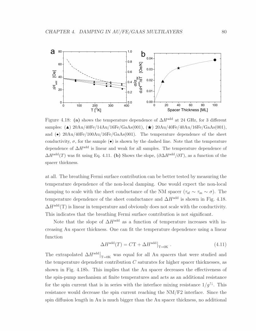
CHAPTER 4. DAMPING IN AU/FE/GAAS MULTILAYERS 80
∆
σσ
∆
Figure 4.18: (a) shows the temperature dependence of ∆Hadd at 24 GHz, for 3 different
samples: () 20Au/40Fe/14Au/16Fe/GaAs(001), () 20Au/40Fe/40Au/16Fe/GaAs(001),
and (•) 20Au/40Fe/100Au/16Fe/GaAs(001). The temperature dependence of the sheet
conductivity, σ, for the sample (•) is shown by the dashed line. Note that the temperature
dependence of ∆Hadd is linear and weak for all samples. The temperature dependence of
∆Hadd(T ) was fit using Eq. 4.11. (b) Shows the slope, (∂∆Hadd/∂T ), as a function of the
spacer thickness.
at all. The breathing Fermi surface contribution can be better tested by measuring the
temperature dependence of the non-local damping. One would expect the non-local
damping to scale with the sheet conductance of the NM spacer (τsf ∼ τm ∼ σ). The
temperature dependence of the sheet conductance and ∆Hadd is shown in Fig. 4.18.
∆Hadd(T) is linear in temperature and obviously does not scale with the conductivity.
This indicates that the breathing Fermi surface contribution is not significant.
Note that the slope of ∆Hadd as a function of temperature increases with in-
creasing Au spacer thickness. One can fit the temperature dependence using a linear
function
∆Hadd(T ) = CT + ∆Hadd∣∣T=0K
. (4.11)
The extrapolated ∆Hadd∣∣T=0K
was equal for all Au spacers that were studied and
the temperature dependent contribution C saturates for higher spacer thicknesses, as
shown in Fig. 4.18b. This implies that the Au spacer decreases the effectiveness of
the spin-pump mechanism at finite temperatures and acts as an additional resistance
for the spin current that is in series with the interface mixing resistance 1/g↑↓. This
resistance would decrease the spin current reaching the NM/F2 interface. Since the
spin diffusion length in Au is much bigger than the Au spacer thickness, no additional

CHAPTER 4. DAMPING IN AU/FE/GAAS MULTILAYERS 81
Sample α [10−3] G [108Hz] ∆H [Oe] 24 GHz
16FesingleRT 4.4 ± 0.2 1.4 37
16FedoubleRT 8.3 ± 0.3 2.6 67
16FedoubleRT -16Fesingle
RT 3.7 ± 0.2 1.15 30
16FedoubleT=0 K-16Fesingle
T=0 K 4.5 ± 0.3 1.41 37
16Fesp 4.47 1.37 36.6
Table 4.2: Table summarizing the damping parameters and linewidth at 24 GHz for the 16
ML Fe film in magnetic single layers and double layers. The values in row 16Fesp show the
prediction from the spin-pump model. Note that the T=0 K values are extrapolated from
Fig. 4.18a.
resistance in Au is expected [132]. The origin of this temperature dependence has not
been resolved yet.
It is worthwhile to point out that the extrapolated value of αadd16Fe
∣∣0K
= 4.5 ±0.2 × 10⁻³ is in excellent agreement with the value estimated from the spin-pumping
theory, αsp16Fe = 4.4 × 10⁻³. This behavior could also be related to the fact that the
spin-pumping theory is strictly valid only at T = 0 K, as outlined in appendix C (see
Eq. C.93).

CHAPTER 4. DAMPING IN AU/FE/GAAS MULTILAYERS 82
4.7 NM Cap Layer as Spin-Sink
4.7.1 Spin accumulation and back-flow
In the previous section the manner in which the injected spin current gets absorbed
by a second ferromagnetic layer was discussed. In this section the relaxation of non-
equilibrium spins inside the NM layer is addressed. In the NM the pumped spin
momentum is relaxed into the lattice by electron momentum scattering in the presence
of spin-orbit interaction. This process requires some degree of spin accumulation in the
NM. For example, in the absence of spin-lattice scattering the accumulated magnetic
moment in the NM creates a back-flow of spin momentum into the ferromagnetic layer.
In equilibrium the back-flow is equal to the pumped spin current [116]. Therefore the
net flow of spin momentum across the F/NM interface is
jnet = jpump − jback. (4.12)
The pumped spin current jpump is given by Eq. 4.4 and an expression for the back-flow
was derived by Tserkovnyak et al. [129] and Urban et al. [122]. The net spin current
crossing the F/NM interface is given by
jnet =
[1 +
τsfg↑↓
hNSlsd tanh(tNM/lsd)
]−1
jpump, (4.13)
where lsd is the spin diffusion length in the NM, N is the density of states per spin in
the NM, tNM is the thickness of the NM layer, and S is the area of the F/NM interface.
The spin diffusion length is defined as lsd =√
Dτsf [129], where τm and τsf are the
electron momentum scattering and spin-flip times, respectively. D = v2F τm/3 is the
electron diffusion constant. In the derivation of Eq. 4.13 the boundary condition for
the F/NM interface was assumed to be given by Eq. 4.12 and the boundary condition
at the outer NM/vacuum interface was jnet(tNM) = 0.
For τsf = 0 there is no back-flow, and the normal metal acts as a perfect spin-
sink. As demonstrated in the previous section, a net spin current flowing out of the
ferromagnet creates additional damping for the precessing magnetization due to the
conservation of angular momentum.

CHAPTER 4. DAMPING IN AU/FE/GAAS MULTILAYERS 83
4.7.2 Induced Gilbert damping
From Eqs. 4.4, 4.8, and 4.13 the additional Gilbert damping constant (taking spin
accumulation into account) is
αspcap =
γg↑↓
4πMStNMS
[1 +
τsfg↑↓
hNSlsd tanh(tNM/lsd))
]−1
. (4.14)
This enhanced Gilbert damping is always smaller than that discussed in section 4.4
(provided that g↑↓ is the same or smaller) since a NM layer on its own is not a perfect
spin-sink. For a free electron gas N = mkF /(2π2
2) and Eq. 4.14 can be rewritten as
αspcap =
γg↑↓
4πMStNMS
[1 +
√3
2√
ε(tanh(tNM/lsd)
−1
]−1
, (4.15)
where ε = τm/τsf is the spin-flip probability per scattering event.
For very small NM thicknesses (tNM lsd) Eq. 4.15 leads to αspcap = 0. The
back-flow of spin momentum from NM compensates the spin-pumping current from
the ferromagnet. This is the reason why the magnetic single layers covered by gold
that were discussed at the beginning of this chapter did not exhibit a spin-pumping
contribution to the damping. When the thickness of the NM is larger than the spin
diffusion length, an additional resistance is created for the spin current. This resis-
tance acts in series with the mixing resistance 1g↑↓ and the effective mixing resistance
may be written as [129]
1
g↑↓eff
=1
g↑↓ + Rsd =1
g↑↓ +lsd
SσNM
e2
h, (4.16)
where Rsd is the resistance per spin (in units of h/e2) for a NM layer with a thickness
equal to the spin diffusion length (tNM = lsd). For infinite thickness the NM cap layer
acts like a partial spin-sink and the saturation value depends on the size of Rsd.
4.7.3 NM cap layer experiments
The role of a NM layer on the non-local damping was studied in magnetic single layer
samples with NM cap layers of various thicknesses. The magnetic Fe layer always had
a fixed thickness of 16 ML. The NM layer was one of Au, Ag, Cu, and Pd, and its
thickness was varied between 0 and 80 nm.
The Au, Ag, and Cu cap layers did not introduce a measurable additional damping
in this range of thicknesses, as illustrated in Fig. 4.19. For Cu, Ag, and Au cap

CHAPTER 4. DAMPING IN AU/FE/GAAS MULTILAYERS 84
α
Figure 4.19: Dependence of the additional damping, αadd, on the cap layer thickness in
NM/16Fe/GaAs(001) samples measured at 23.9 GHz. The NM was one of Au (), Cu (),
Ag ( ), and Pd (•). The dotted line is a fit to the Pd data using Eq. 4.15 and the solid line
is a fit using Eq. 4.21.
∆ ∆
Figure 4.20: (a) Frequency dependence of ∆H and (b) temperature dependence of ∆H at
23.9 GHz for the 50Pd/16Fe/GaAs sample.
layers the linewidth changed by less than 2 Oe which corresponds to the experimental
uncertainty of the linewidth measured at 24 GHz.
The situation was found to be very different for Pd cap layers, in this case the
linewidth rapidly increased with the Pd thickness and saturated at tPd ≈ 10 nm. The
magnitude of this increase was comparable to that produced by the intrinsic damping,
and the corresponding frequency dependence (see Fig. 4.20a) clearly showed that the

CHAPTER 4. DAMPING IN AU/FE/GAAS MULTILAYERS 85
additional linewidth scaled with the microwave frequency with no appreciable zero
frequency offset (2 Oe). The linear frequency dependence justifies the interpretation
of the increase in linewidth as an additional Gilbert damping parameter (see Fig. 4.19).
Equation 4.15 provides an analytic expression for the enhanced damping parame-
ter as a function of the NM thickness assuming diffusive electron transport. Since the
additional damping occurred for very small NM thicknesses, the use of spin diffusion
theory is questionable.
A simple estimate for g↑↓/S can be obtained from the density of electrons using
Eq. 4.6. Andersen [133] estimated the number of conduction electrons per Pd atom
to be 0.37. This implies a carrier density of n = 2.5 × 1022 cm−3 and leads to
g↑↓/S = 0.65×10¹⁵. This number is reasonable when compared to the values for g↑↓/S
calculated from first principles for Cu/Co interfaces, in which case Xia et al. [118]
found g↑↓/S = 1.1 × 10¹⁵. One expects g↑↓/S to be smaller for Pd than for Cu since
Pd has a smaller number of conduction electrons per atom than Cu.
g↑↓/S = 0.65 × 10¹⁵ cannot explain the data in Fig. 4.19 since the resulting
saturation value is too low. A reasonable fit requires g↑↓/S = 1.2 × 10¹⁵, ε = 4,
and lsd = 5.1 nm (dotted line). ε = 4 means that it is four times more likely for
an electron in Pd to flip its spin than to change its momentum upon scattering and
renders Eq. 4.13 invalid. The saturation value of the enhanced Gilbert damping was
αadd = 3.5× 10⁻³ which is close to the additional damping found in magnetic double
layers (see section 4.3).
Validity of the spin diffusion theory for Pd
To explain the experimental results with NM=Pd it was necessary to use values for ε
bigger than 1. This is not compatible with the spin-diffusion equation, and the spin
transport in the Pd layer cannot really be described as diffusive.
To gain further insight, the electron mean free path in the Pd layer was deter-
mined from the resistivity. To accomplish this, the sheet resistances of two samples
20Au/50Pd/16Fe/GaAs and 20Au/16Fe/GaAs were measured by means of the van
der Pauw technique [134]. The resistances were found to be 9.6 Ω and 19.9 Ω
, re-
spectively. Since the individual layers contribute in parallel, one can infer that the
sheet resistance of the isolated 50 ML Pd film was 18.7 Ω. Using a Pd thickness of 9.7
nm (50 ML), the resistivity of the Pd layer would be = 18.2 µΩcm which is almost
double the resistivity of bulk Pd (Pd = 10.8 µΩcm [23]). The measured resistance
CHAPTER 4. DAMPING IN AU/FE/GAAS MULTILAYERS 86
allows one to estimate an effective electron momentum scattering time τm in the Pd
layer from the relation1
=
e2nτm
m∗ , (4.17)
where e is the elementary charge, m∗ the effective mass, and n the density for conduc-
tion electrons. The electron mean free path is given by λm = vF τm, the effective mass
of the conduction electrons in Pd is m∗ ≈ 2m, and the Fermi velocity is vF = 5.6×10⁷
cm/s [135]. It follows that λm ≈ 8.6 nm. Since this number is bigger than the spin
diffusion length (obtained from fitting Eq. 4.14 to the data) and the film thickness
the diffusive theory is clearly not applicable.
4.7.4 Alternate model of spin transport in Pd
Bulk Pd is a strongly enhanced paramagnet with a large Stoner enhancement factor
and known to be on the verge of ferromagnetism with locally fluctuating magnetic
moments (paramagnons) [136, 137, 138, 139]. One could imagine that these fluctuat-
ing moments act as very effective spin scatterers. The spin current which is injected
into the NM by the precession of the magnetization interacts with these paramagnons
and the spin-spin scattering leads to a local randomization of the direction of the spin
momentum of the spin current [140]. This randomization represents a loss of (lateral)
coherence of the spin current and is reminiscent of ‘mode-mode coupling’. On average
the spins travel the spin-flip length λs, before their initial spin momentum is flipped.
This length is not equivalent to the spin diffusion length since it is not assumed that
electrons experience a number of momentum scattering events before their spin is
flipped.
Thus the spin current injected into the Pd layer (jpump) will gradually loose its
coherence as a function of the Pd thickness and the angular momentum is effectively
absorbed. This means that different locations of the F/NM interface accept the back-
flow of spin momentum with a randomized phase. The exchange interaction in Fe
averages these local contributions and consequently the net back-flow approaches zero
with increasing Pd thickness. The magnitude of the coherent spin current returning
to the Fe layer, jback, is given by the amount of spin current that is not lost as the
electrons make a round trip through the Pd layer. Since the electrons can move
in arbitrary directions from the F/NM interface an effective layer thickness Leff is
introduced. Leff is an effective NM layer thickness which is averaged over all available

CHAPTER 4. DAMPING IN AU/FE/GAAS MULTILAYERS 87
in-plane electron momenta k‖ up to the Fermi wave vector kF with an appropriate
weighing. One can write [141]
πk2F
(2π)2e−
Leffλs =
∫ kF
0
2πk‖dk‖(2π)2
e−tNMcos θ
1λs , (4.18)
with cos θ =√
1 − (k‖kF
)2, where θ is the direction of the electron momentum measured
with respect to the surface normal. Therefore the back-flow is
jback = jpumpe− 2Leff
λs . (4.19)
An additional factor of 2 appears in the exponent, because the average distance trav-
elled by spins that make it back into the ferromagnet after a round trip through the
Pd layer is 2Leff . The net spin current through the NM/F interface is then given by
jnet = jpump
(1 − e−
2Leffλs
). (4.20)
Using this in Eq. 4.14 one arrives at a new expression for the enhanced Gilbert damp-
ing
αspcap =
γg↑↓
4πMStFeS
(1 − e−
2Leffλs
). (4.21)
Now the Pd data in Fig. 4.19 can be fit again using Eq. 4.21. This fit determines only
two truly independent parameters. As seen in Fig. 4.19, the fit describes the Pd data
very well, resulting in g↑↓/S = 0.9 × 1015 cm−2. This value is significantly smaller
than that determined by fitting the data to the diffusion theory, and is approximately
equal to the value estimated from the conduction electron density in Pd. This model
does not allow for spin accumulation so that Pd acts as a perfect spin-sink when
thick enough. From the fit, the spin mean free path λs was determined to be λs =
9.0 nm. This implies that the spin mean free path is only slightly bigger than the
electron mean free path calculated from the conductivity, λm = 8.6 nm. This is an
unusual situation and may be a consequence of electron-electron correlation effects
occurring in Pd. Recently, Kurt et al. also observed a very short spin-flip length
in Pd at low temperatures [142]. Using current perpendicular to the plane (CPP)
GMR measurements, they found λPds = 25± 7 nm at 4 K. The discrepancy between
this value and the λs estimated from FMR very likely has two origins: (i) λs at
low temperature is usually longer than at RT; in simple metals the spin-flip length
decreases by a factor of 2 between 4 K and 300 K [143, 144]; (ii) CPP GMR measures

CHAPTER 4. DAMPING IN AU/FE/GAAS MULTILAYERS 88
the longitudinal spin-flip length while FMR is sensitive to the transverse spin-flip
length.
The lack of a pronounced temperature dependence for ∆Hadd with NM=Pd (see
Fig. 4.20b) supports the conjecture that the scattering of the spin current in Pd is
due to temperature independent electron-electron correlation effects.
4.8 Spin-Pumping in Other Experiments
4.8.1 Single layers
Heinrich et al. [24] reported FMR line broadening for very thin Fe films grown on
Ag(001) substrates. In this case the damping parameter increased from α = 2.1×10⁻³
for a film having a thickness of 24 ML to α = 18.2 × 10⁻³ for a 4 ML thick film. In
light of the fact that the thicker film exhibited a damping parameter very close to
the intrinsic value for bulk Fe [145], it is likely that only a very small fraction of the
increased damping in the thinner film was due to spin-pumping. One can therefore
conclude that Ag is a very poor spin-sink. More recently, Platow et al. [146] measured
the thickness dependence of the FMR linewidth for Ni grown on Cu(001). In this
experiment Cu also provided a very poor spin-sink.
Mizukami et al. [147, 130] conducted a systematic FMR study of the NM/Py/NM
system prepared by sputtering on glass substrates, where the NM was Cu, Ta, Pd,
and Pt. The thickness of the NM cladding layers was held fixed at 50 A while the
thickness of the Permalloy layer was varied between 20 and 100 A. For Cu and Ta
cladding layers the damping parameter for Py was equal to its intrinsic value and
independent of the Py thickness. Pd and Pt cladding layers however caused a strong
increase in damping such that the additional damping increased with the inverse Py
thickness. For NM=Pd the effect was 40% stronger than in the studies presented
in this thesis (taking into account two interfaces and the lower magnetization of Py
relative to Fe). In a subsequent paper Mikazumi et al. investigated the FMR line
broadening of a 30 A Py layer due to the proximity of a Pt layer [148, 149]. In this
case a 50 A Pt layer was spatially separated from the Py layer by a Cu spacer of
variable thickness. For Cu spacer thicknesses less than 100 nm, the Pt layer resulted
in a measurable line broadening. With the thinnest Cu spacer (3 nm) the strength of
the enhanced damping agrees in magnitude with the enhanced damping observed in

CHAPTER 4. DAMPING IN AU/FE/GAAS MULTILAYERS 89
the 50Pd/16Fe/GaAs(001) system, and is presumably due to spin-pumping effects.
4.8.2 Double layers
The spin-pumping effect also has profound consequences for the dynamics of exchange
coupled magnetic bilayers. Coupled bilayers have acoustic and optic precessional
modes [4]. Using Eq. 4.9 and including exchange coupling terms one can calculate
the effect of spin-pumping and exchange coupling. For example for a 5Fe/12Cu/10Fe
bilayer with no interlayer exchange coupling, the calculated spin-pumping contribu-
tion to the FMR linewidth at 36 GHz is 150 Oe for the 5Fe film and 75 Oe for the
10Fe film. By turning on a moderate antiferromagnetic exchange coupling J = −0.2
erg/cm2 the optical peak is broadened by 200 Oe while the acoustic peak is broadened
by only 36 Oe. For moderate antiferromagnetic exchange coupling the optical peak
mainly arises from the 5Fe layer (with J = −0.2 erg/cm2 one has mrf5Fe/m
rf10Fe = 3.6
at 36 GHz). It is not surprising that the 5Fe peak broadens further in the presence of
exchange coupling, considering that the optical mode corresponds to an out-of-phase
precession of the magnetic moments of the 5Fe and 10Fe layers. In this case the spin
momentum is more efficiently pumped between the two layers and results in more
damping. By the same argument, the in-phase precession of the moments for the
acoustic peak (10Fe) narrows the FMR line of the acoustic mode.
Experimentally, optical FMR peaks were always observed to be wider than the
acoustic peaks. In a 5Fe/12Cu/10Fe sample grown on a Ag(001) substrate the
linewidth of the optical peak was found to be enhanced by as much as 500 Oe compared
to the single layer [150]. This indicates that approximately 50% of this broadening
was due to spin-pumping and the reminder was caused by an inhomogeneous exchange
coupling [121].
Recently, Lubitz et al. [151] also found an increase of the FMR linewidth in thin
polycrystalline Fe films grown on Silicon which was induced by Cu/Fe cap layers.
These measurements are in qualitative agreement with the Fe/Au/Fe/GaAs double
layer results presented in section 4.3, but the thickness dependent FMR linewidth ob-
served for their polycrystalline Fe single layers [151] makes a quantitative comparison
difficult.
Chapter 5
Two-Magnon Scattering
5.1 Au/Pd/Fe/GaAs Multilayers
The resonance linewidth in Au/Pd/Fe/GaAs(001) multilayers was observed to exhibit
a strong extrinsic contribution. This effect will be discussed in terms of the two-
magnon scattering model in this chapter.
5.1.1 Growth, RHEED, STM, TEM studies
The Pd(001) in-plane lattice constant has a large mismatch of 4.4% with respect to
the Fe(001) template, even when [110]Pd ‖ [100]Fe. Au grows over Pd with the in-plane
cubic axes parallel to each other ([100]Au ‖ [100]Pd). The Pd and Au lattice spacings
are mismatched by 4.5 percent. The presence of Pd in crystalline Au/Pd/Fe(001) mul-
tilayers provides a large lattice strain which, above a critical Pd thickness, is relieved
by the formation of misfit dislocations. Results in this section are mainly presented
for the magnetic single layer nPd/30Fe/GaAs(001) and Au/nPd/16Fe/GaAs(001)
films, where n was varied between 0 and 300 ML.
The RHEED pattern for the Au(001) cap layer in 20Au/nPd/16Fe/GaAs(001) de-
pends on the number of atomic layers of Pd, n. For n < 4 the RHEED patterns of the
Au(001) surface layers were similar to those observed for case of Au/Fe/GaAs(001),
as shown in Fig. 4.2. For n ≥ 4 the RHEED patterns for Au(001) developed fan-out
streaks when the primary electron beam was oriented along the 〈100〉Au directions (see
Fig. 5.1a). The intensity of this effect saturated for n ≥ 9. Fan-out RHEED streaks
are a well known feature in MBE epitaxy. It has been shown by Pukite [76, 77]
90

CHAPTER 5. TWO-MAGNON SCATTERING 91
Figure 5.1: (a) Shows a RHEED pattern with strong fan-out features (indicated
by arrows) on the surface of Au(001) due to a network of misfit dislocations in
20Au/9Pd/16Fe/GaAs(001). The electron beam was oriented along the [100]Au direction.
Note that in this orientation the RHEED streak intensities which are caused by the As
2 × 2 surface reconstruction are significantly diminished in the presence of misfit disloca-
tions (cf. Fig. 4.2b), indicating that the long range order of the surfactant As in the [100]
directions deteriorated. (b) The primary electron beam was oriented along the [110]Au
direction. No fan-out streaks are visible.
that their presence is related to surface clustering involving rectangular symmetry, as
outlined in section 3.1.3. Pukite’s result allows one to make the following practical
conclusion: The presence of RHEED fan-out streaks with 90 symmetry is due to the
formation of a rectangular network of surface line defects. For the RHEED electron
beam oriented at 45 with respect to the direction of line defects the fan-out streak
pattern is symmetric and reaches its maximum intensity; while for an electron beam
oriented along the line defects (for angles 0 and 90) only simple straight streaks are
present. This is exactly what is observed, as shown in Fig. 5.1.
The rectangular network of line defects on the surface is caused by nucleation
and glide of misfit dislocation half-loops entering the crystal surface during the film
growth to compensate for the lattice mismatch. This gliding of dislocations along the
111Pd,Au planes is illustrated in Fig. 5.3.
From the RHEED patterns shown in Fig. 5.1a it can be concluded that the surfaces
of the Au/nPd/Fe/GaAs(001) structures with n ≥ 9 consist of a network of line
defects, which are oriented along the 〈110〉Au crystallographic directions of Au(001).

CHAPTER 5. TWO-MAGNON SCATTERING 92
Figure 5.2: Ex-situ 1500 A × 1500 A STM images of (a) 90Au/16Fe/GaAs(001) and (b)
90Au/9Pd/16Fe/GaAs(001). The arrows along the 〈110〉Au directions highlight surface
steps which are caused by the dislocation glide. The z-scale (from white to black) in
both images is 8 A, and the RMS roughness was ∼ 1 A. (c) Plan view TEM image of
the 90Au/9Pd/16Fe/GaAs(001) sample. The black arrow indicates the [110]Au crystallo-
graphic direction and the contrast that exhibits a clear four-fold symmetry (parallel and
perpendicular to the arrow) is due to the misfit dislocation network. The features oriented
at 45 with respect to the [110]Pd direction indicated by the white arrows are caused by
moire fringes [152]. The inset shows the corresponding electron diffraction pattern. The
intensity connecting diffraction spots parallel to the 〈110〉Au directions give a hint to the
defects.
These line defects correspond to atomic steps caused by the intersection of the 111Au
glide planes with the surface [153, 154]. This conjecture is further confirmed by STM

CHAPTER 5. TWO-MAGNON SCATTERING 93
studies of the Au(001) layer of the 90Au/9Pd/16Fe/GaAs(001) sample. Fig. 5.2b
shows surface steps arising from the network of misfit dislocations, indicating that
the atomic displacements along the 111Au glide planes propagate through the top
Au layer.
Figure 5.3: Dislocation
half loops on a 111 glide
plane.
The presence of a self-assembled network of misfit dis-
locations was observed using transmission electron mi-
croscopy (TEM) by plan view orientation of the layer sys-
tem 90Au/9Pd/16Fe/GaAs(001), (see Fig. 5.2c). The ob-
served orientation and density of the dislocation arrange-
ment resembles the misfit dislocation network observed
by Jorg Woltersdorf in epitaxially grown Au/Pd bicrys-
tals [155, 152] of the corresponding thicknesses. During
the growth of the first Pd monolayers on the Au(001) sub-
strate, complete misfit dislocations are generated and form
a rectangular network located at the Pd/Au interface. Af-
ter reaching the critical thickness of 4 ML, the process of gliding of substrate disloca-
tions can no longer produce a sufficiently high density of dislocations to compensate
the misfit; thus additional dislocation half loops are generated [156, 157] starting at the
top Pd layer and extending to the interface, as illustrated in Fig. 5.3. The correspond-
ing interference of moire patterns and dislocation contrast phenomena treated in [152]
is also recognizable in Fig. 5.2c, as indicated by the white arrows. The mechanisms
for generation of interface dislocations and their efficiency for misfit compensation
was outlined in [158].
5.1.2 FMR studies
The magnetic anisotropies of the Fe(001) layer in nPd/30Fe/GaAs(001) and in
Au/nPd/16Fe/GaAs(001) were similar to those observed for dislocation free Au/Fe/-
GaAs(001) systems of the corresponding thicknesses [110]. The easy axes of the 30Fe
layer were oriented along the 〈110〉Fe directions due to the in-plane uniaxial anisotropy
originating at the GaAs interface [110]. The striking difference between the samples
having a thick Pd layer in nPd/Fe/GaAs(001), n ≥ 130, and those with n ≤ 110 was
in the level of magnetic damping. The Fe layers in nPd/Fe/GaAs(001) structures
with n ≤ 110 exhibited only Gilbert damping enhanced by spin-pumping of the Fe
layer and having a spin-sink inside the Pd layer, as described in section 4.7.3 and

CHAPTER 5. TWO-MAGNON SCATTERING 94
Figure 5.4: Typical FMR spectra measured at 23.9 GHz on the 200Pd/30Fe/GaAs(001)
sample. The left spectra were taken with the magnetization M in the plane: M ‖ [100]Fe
(solid line) and M ‖ [110]Fe (dotted line). The right spectrum corresponds to the per-
pendicular configuration (M ‖ [001]Fe). Note that the FMR linewidths for the in-plane
configuration are anisotropic, and the narrowest line is measured in the perpendicular con-
figuration.
[159, 140]. The FMR linewidth in nPd/Fe/GaAs(001) samples with n ≥ 130, was
different. In these samples the FMR linewidth was strongly dependent on the an-
gle ϕM between the magnetization and the crystallographic 〈100〉Fe axes, showing a
distinct four-fold symmetry, as can be seen in Fig. 5.5. The minima and maxima in
∆H are along the 〈110〉Fe and 〈100〉Fe crystallographic directions, respectively. It is
interesting to note that ∆H(ϕM) does not show a two-fold symmetry. This implies
that the chemical bonding between Fe and the uniaxial dangling bonds of GaAs at
the Fe/GaAs(001) interface is not important for the formation of magnetic defects
by the network of misfit dislocations. The FMR linewidth also changed in a very
pronounced way as a function of microwave frequency. The frequency dependence
of the FMR linewidth, ∆H(f), along the 〈100〉Fe and 〈110〉Fe directions is shown in
Fig. 5.6. Along the 〈110〉Fe (easy magnetic axes) and 〈110〉Fe (hard magnetic axes),
the FMR linewidth is nearly linearly dependent on the microwave frequency between
10 and 73 GHz, but is accompanied by a zero frequency offset ∆H(0) = 50 Oe.
The slope of ∆H(f), however, is nearly that corresponding to the intrinsic Gilbert
damping (including spin-pumping into a 100Pd(001) cap layer [140]) obtained in the

CHAPTER 5. TWO-MAGNON SCATTERING 95
Figure 5.5: The ferromagnetic resonance linewidth for the 200Pd/30Fe/GaAs(001) film at
73(), 36(•), and 24() GHz as a function of the in-plane angle ϕM between the magne-
tization and the [100]Fe axis. The angles ϕM were calculated from ϕH using the magnetic
anisotropies and the applied field; the dotted lines indicate the ∆H due to the intrinsic
damping (including spin-pumping) at 73.0, 36.4, and 23.9 GHz.
samples without extrinsic damping. ∆H was quite different when measured with the
saturation magnetization along the 〈100〉Fe directions. Note that for the 30 ML thick
Fe film the 〈100〉Fe directions are neither easy nor hard magnetic axes, and therefore
it is not possible to avoid dragging of the magnetization behind the applied external
field at FMR. ∆H was determined by finding the in-plane external field angle, ϕH ,
which corresponds to M ‖ 〈100〉Fe at resonance. The open circles in Fig. 5.6 show
this measured linewidth. Dragging the magnetization behind the external field, how-
ever, results in additional FMR line broadening. This effect is usually present at low
frequencies, because the FMR fields become comparable to the in-plane anisotropy
fields. Dragging was nearly absent at and above 24 GHz. In order to remove the
dragging contribution at 10 and 14 GHz, the FMR linewidth was evaluated in the
following manner: FMR peaks were calculated including dragging of the magnetiza-
tion, and the effective Gilbert damping (αeff) was adjusted in such a way that the
total ∆H was equal to that observed experimentally (open circles). Then the FMR
linewidths without the dragging contribution were obtained using the effective Gilbert
damping (∆H = 2πfγ
αeff). These are shown as the filled points in Fig. 5.6. The fol-
lowing features can are noteworthy: (i) The dependence on the microwave frequency,

CHAPTER 5. TWO-MAGNON SCATTERING 96
Sample ∆H〈100〉 [Oe] ∆H〈110〉 [Oe]
200Pd30FeGaAs 180 75
90Au10Pd16FeGaAs 210 60
20Au40Fe40Au9Pd16FeGaAs 175 50
20Au40Fe40Au9Pd16FeGaAs 160 50
20Au40Fe40Au4Pd[FePd]514FeGaAs 123 55
20Au40Fe40Au4Pd[FePd]514FeGaAs 123 55
20Au40Fe[PdFe]54Pd40Au4Pd[FePd]514FeGaAs 200 50
20Au 40Fe[PdFe]54Pd40Au4Pd[FePd]514FeGaAs 120 45
20Au40Fe40Pd16FeGaAs 210 75
20Au40Fe40Pd16FeGaAs 75 75
20Au20Fe40Pd16FeGaAs 210 75
20Au20Fe20Pd16FeGaAs 75 75
Table 5.1: Summary of the anisotropic FMR linewidths for samples with a network of
misfit dislocations measured at 23.9 GHz. The data correspond to the magnetic layer that
is highlighted in bold.
∆H, is not described by a simple linear dependence on the frequency as would be
expected for Gilbert damping. (ii) The slope of the FMR linewidth vs. frequency is
nearly that expected for the intrinsic damping for frequencies between 36 and 73 GHz,
but ∆H(0) = 160 Oe is significantly increased compared to the 〈110〉Fe orientations.
(iii) For frequencies less than 36 GHz the frequency dependence of ∆H shows a clear
downturn (see Fig. 5.6).
A similar frequency dependence for ∆H was found recently by Twisselmann et
al. [160] for Permalloy (Py) films grown on NiO and Lindner et al. [161] for Fe/V
superlattices. In fact, the frequency dependence observed along the 〈100〉Fe orienta-
tions resembles recent calculations by Arias and Mills [162] of extrinsic damping due
to two-magnon scattering, as shown by the thin solid line in Fig. 5.6. The Arias-Mills
model result was calculated using Eq. 2.55. It does not exhibit sufficient downturn
at low frequencies, likely because it is not applicable to the present case since a very
different defect model was assumed (spatial variation of the direction of the uniaxial
perpendicular anisotropy [12]).
The increase of the FMR linewidth noted above has been observed in several dif-
ferent sample structures involving a lattice mismatched layer of Pd. In Tab. 5.1 the
linewidths measured along the 〈100〉Fe and 〈110〉Fe directions are summarized for sev-

CHAPTER 5. TWO-MAGNON SCATTERING 97
∆
Figure 5.6: The frequency dependence of the FMR linewidth for the
200Pd/30Fe/GaAs(001) structure along the 〈110〉Fe () and 〈100〉Fe (•) directions,
respectively. () points show ∆H along 〈100〉Fe before the dragging contribution to the
linewidth was removed (see further details in the text). The purpose of the thick solid line
spline fit is to guide the eye. The thin solid line corresponds to the calculated frequency
dependence of ∆H, using Eqs. 2.55 and 2.47 (Arias and Mills model [12]). The dashed
line shows the frequency dependence of the intrinsic FMR linewidth (Gilbert damping)
obtained by using the 100Pd/30Fe/GaAs(001) sample with no magnetic defects in the Fe
film. The spin-pumping contribution in 100Pd/30Fe/GaAs(001) to ∆H is saturated (see
Fig. 4.19). The -symbols on the dashed line show the FMR linewidth in the perpendicular
configuration at 9.7 and 23.9 GHz for the 200Pd/30Fe/GaAs(001) sample. Note that the
-symbols are right on the dashed line, indicating that in the perpendicular configuration
the FMR linewidth ∆H is given by the Gilbert damping (α = 0.006) with no zero frequency
offset (∆H(0)⊥ = 0). The dotted lines indicate the range of microwave frequencies where
the slope of ∆H(f) nearly corresponds to Gilbert damping. Note that the dotted lines
have zero frequency offsets.
eral samples. All samples had one thing in common: extrinsic damping was triggered
by lattice defects which are caused by the misfit dislocation network. The onset of two-
magnon scattering required a critical thickness of Pd and this critical value depends on
where the Fe layer is located. For an Fe layer deposited on the Pd spacer, the critical
thickness for the onset of two-magnon scattering is equivalent to the critical thickness

CHAPTER 5. TWO-MAGNON SCATTERING 98
for the formation of misfit dislocations in Pd with n ≥ 4 [155]. The area density
of misfit dislocations [155] and the magnitude of two-magnon scattering saturate for
n ≥ 9. For Fe layers grown directly on GaAs(001), the formation of magnetic defects
required either a thick Pd layer (n > 130) or a combination of a thin Pd (n ≥ 9) and a
thick Au layer (> 70); e.g. 90Au/9Pd/16Fe/GaAs(001) or 200Pd/30Fe/GaAs(001).
In all samples the strength of the two-magnon scattering was found to be nearly in-
dependent of the thickness of the Fe. This implies that the two-magnon scattering
is a bulk effect for the range Fe thicknesses studied (10 to 40 ML). This behavior
can be expected in good crystalline films; once dislocation half loops are generated,
they propagate along the 111Pd glide planes and are terminated at the outer in-
terfaces. The extrinsic damping in all the samples listed in Tab. 5.1 exhibited a
similar qualitative and quantitative behavior as a function of microwave frequency
and magnetization angle. Since spin-pumping in magnetic bilayers affects the angu-
lar dependence of the FMR linewidth due to accidental crossovers of the resonance
fields [159], the discussion will be now limited to the simple 200Pd/30Fe/GaAs(001)
magnetic single layer sample.
5.1.3 Two-magnon scattering model
Two-magnon scattering, if applicable, can provide a simple model for the description
of extrinsic damping in FMR. Inhomogeneous magnetic properties generate scattering
of the resonant mode (uniform mode with q ∼ 0) into non-uniform modes (q = 0
magnons), as discussed in section 2.5. From Eq. 2.48 it follows that magnon scattering
is confined to degenerate magnons following the path of lobes, q0(ψq), around the
direction of the magnetic moment (see Fig. 5.7).
Two-magnon scattering formally enters the in-plane rf susceptibility [12] as an
additional term R in the denominator (cf. Eq. 2.53)
χ|| =MsB
BeffH − (ωγ)2 + i(H + B)αω
γ+ [(R) + i(R)]
, (5.1)
where Beff = H+4πMeff is the effective magnetic induction, and the in-plane anisotro-
pies are neglected for simplicity. The real part, (R), leads to a shift in the FMR
field and the imaginary part (R) provides additional damping. (R) and (R)
have to satisfy the symmetry of the magnetic inhomogeneities. In a rectangular
network of misfit dislocations one expects to get additional four-fold anisotropies,

CHAPTER 5. TWO-MAGNON SCATTERING 99
M
[010]
[10
0]
M
Figure 5.7: The black lines show the lobes of degenerate magnons calculated for 73 GHz
(big lobes) and 24 GHz (small lobes). The background is a contour plot of the in-plane
Fourier components from Eq. 3.12. Note that Pukite’s type of I(q), even if it were scaled
to produce an anisotropic behavior for small q-vectors (large 〈L〉), would result only in a
weak anisotropy for ∆H.
affecting both the FMR field and magnetic damping. In addition both, (R) and
(R) are dynamic effects and depend on the microwave frequency. This leads to
an important conclusion: Magnetic anisotropies measured using FMR can have a
frequency dependent contribution which is absent in dc measurements.
The strength of two-magnon scattering as a function of the angle ϕM of the magne-
tization with respect to the in-plane crystallographic axis can be tested by inspecting
the expression (R). The imaginary part of the two-magnon contribution to the
susceptibility is proportional to the Fourier components of the scattering potential.
Using this one can write
[R(ϕM)] ∼∫
I(q‖)δ(ω − ωq‖)dq2‖ = 2
ψmax∫−ψmax
I(q0, ϕq, ϕM)q0dψq
∂ω∂q
(q0, ψq), (5.2)

CHAPTER 5. TWO-MAGNON SCATTERING 100
ϕ
Figure 5.8: The FMR fields for the 30Fe layer in 200Pd/30Fe/GaAs(001) as a function
of the in-plane angle ϕH . Where ϕH = 0 corresponds to the [100]Fe direction. Mea-
surements were carried out at 73.0( ), 36.4(), 24.9(), and 14.1() GHz. The solid
lines were calculated using the following parameters: The effective demagnetizing field
4πMeff = 18.7 kG, in-plane uniaxial field 2K ||U/MS = −360 Oe, four-fold in-plane anisotropy
field 2K‖1/MS = 330 Oe, and g-factor, g = 2.11. The uniaxial in-plane anisotropy has the
hard axis along the [110]Fe direction. With these parameters the agreement between the
measured and calculated FMR fields along the 〈110〉Fe direction is within 10 Oe for all
frequencies. This is not true when the field applied along the 〈100〉Fe directions where the
discrepancy is of the order of 100 Oe. It is not possible to get a perfect fit for all microwave
frequencies by using a single set of parameters, indicating that the magnetic anisotropies
are partly frequency dependent.
where I(q‖) represents the intensity of two-magnon scattering, and ϕq = ϕM + ψq
is the angle of the q‖ vector with respect to the [100]Fe (defect) axis. The magnon
group velocity ∂ω∂q
(q0, ψq) in Eq. 5.2 is proportional to the strength of the dipolar and
exchange fields and represents the dipole-exchange narrowing of local inhomogeneities
[49]. The term q0∂ω∂q
(q0,ψq)describes a weighting parameter along the path of the two-
magnon scattering lobes q‖(ψq). It turns out that for a given microwave frequency
this factor is nearly independent of ψq. This means that the whole two-magnon scat-

CHAPTER 5. TWO-MAGNON SCATTERING 101
tering lobe contributes to (R) with an equal weight, independent of the angle ψq.
The exception is the q-space close to the origin of the reciprocal space. It is important
to realize that long wavelength (small q) variations in magnetic properties lead to a
simple superposition of local FMR peaks. The extrinsic FMR linewidth in this case
merely reflects large length scale sample inhomogeneities and should not be treated
by two-magnon scattering. McMichael et al. [160] concluded that the FMR linewidth
is given by a superposition of local resonances when the characteristic inhomogeneity
field is larger than the interaction field [163]. In the range of long wavelength defects
the important part of the interaction field between grains having different magnetic
properties is the magneto-static contribution 2πMsqtF to the magnon energy dis-
persion, where tF is the film thickness. The FMR spectrum is given by a simple
superposition of local FMR peaks when
HpL ≥ 3πMstF , (5.3)
where Hp is the root mean square value of random variations of a local anisotropy
field satisfying a Gaussian distribution, and L is the average grain size (see Fig. 4 in
[164]). The summation of local FMR signals can result in a genuine zero frequency
offset ∆H(0), (see reference [164]).
The critical angle ψmax appearing in Eq. 5.2 decreases with a decreasing angle θM
of the magnetization with respect to the sample plane. For θM ≤ π/4 no degenerate
magnons are available [56]. The angle θH satisfying θM ≤ π/4 has to be calculated
by minimizing the total magnetic energy. For the 200Pd/30Fe/GaAs sample this
angle was θH = 12 at 24 GHz, as can be seen in Fig. 5.10. This is an important
criterion that allows one to test the applicability of two-magnon scattering to the
interpretation of extrinsic damping. ∆H from the extrinsic damping has to disappear
when the direction of the magnetization is in the vicinity of the film normal. It is
interesting to note that the weighing parameter q0∂ω∂q
(q0,ψq)is nearly independent of θM .
It increases somewhat very close to the critical angle θM = π/4, where the two-magnon
scattering is switched off.
5.1.4 Discussion of the FMR linewidth
The dependence of the FMR field and linewidth on the angle θH between the dc
magnetic field and the sample normal is shown in Fig. 5.9. The data in Fig. 5.9b
show that the damping decreases significantly in the vicinity of the perpendicular

CHAPTER 5. TWO-MAGNON SCATTERING 102
θ
∆
θ
Figure 5.9: (a) The ferromagnetic resonance field in the 30Fe layer in 200Pd/-
30Fe/GaAs(001) as a function of the angle θH between the sample normal and the applied
field H measured at 24 GHz. The the magnetic field was rotated in the (001) plane. The
parameters used for to fit the data are as follows: 4πMeff = 20.6 kG, 2K||1 /MS = 330 Oe,
2K||U/MS = −360 Oe, 2K⊥
1 /MS = −350 Oe, and g =2.02. The in-plane anisotropy fields
were determined from FMR measurements in the parallel configuration (see Fig. 5.8). The
dashed line shows the fit obtained by fixing 4πMeff , 2K||1 /MS , 2K
||U/Ms, and g factor to the
values from the in-plane FMR measurements (see a list of these parameters in the caption
of Fig. 5.8). The only adjustable parameter is 2K⊥1 /Ms = −700 Oe. (b) Ferromagnetic
resonance linewidth, ∆H, as a function of θH at 23.9 GHz. The dots represent the measured
data and the dashed line represents the FMR linewidth ∆HG(θ) that was calculated using
the Gilbert damping from the perpendicular configuration. The peak in the FMR linewidth
for θH = 12 is caused by the dragging of the magnetization behind the applied field.
configuration. In fact, the measured ∆H in the perpendicular configuration at 10
and 24 GHz was given exactly by the intrinsic damping, as previously illustrated in
Figs. 5.4, 5.6, and 5.9b.
The strength of two-magnon scattering as a function of θH is usually expressed in
terms of the adjusted frequency linewidth [53]
∆ω
γ=
(dω
dH
)∆Hext(θH) , (5.4)
where dω/dH = [ω(H + ∆H, θH + ∆θH) − ω(H, θH)]/∆H using the FMR condition
for the resonance frequency which includes the in-plane and out-of-plane magnetic
anisotropies. It is more convenient to calculate dω/dH by picking ∆ω and evalu-
ating the corresponding change in ∆H and ∆θH satisfying the resonance condition.

CHAPTER 5. TWO-MAGNON SCATTERING 103
∆ω/γθ
θ
Figure 5.10: (•) represents the adjusted frequency FMR linewidth ∆ω/γ from the extrinsic
contribution as a function of θH at 23.9 GHz. The solid line shows the angle of magnetization
θM as a function of θH . The dashed line shows the critical angle ψmax as a function of θH .
Notice that ψmax describes the angular dependence of ∆ω/γ quite well. ψmax was scaled in
order to compare it with ∆ω/γ.
The difference between the measured linewidth ∆H(θH) and the linewidth predicted
∆HG(θH), using intrinsic Gilbert damping, determines the contribution arising from
the extrinsic damping, ∆Hext(θH) = ∆H(θH) − ∆HG(θH).
The dots in Fig. 5.10 show that the angle θM at which the two-magnon contri-
bution rapidly disappears is in excellent agreement with the theoretical prediction of
π/4. This behavior was found in all samples affected by the network of misfit disloca-
tions. The extrinsic damping contribution remains nearly constant as a function of θH
until the direction of the magnetic moment is in the vicinity of π/4 where it abruptly
collapses to zero, as shown in Fig. 5.10. Fig. 5.9b shows that the FMR linewidth in
the vicinity of the perpendicular configuration is given entirely by Gilbert damping.
It follows that the extrinsic damping generated by a self-assembled network of misfit
dislocations can be described by the two-magnon scattering mechanism. Since the
angular dependence of ∆ω(θH)/γ is virtually traced by ψmax(θH) one can conclude
that the two-magnon scattering intensity I(q, θH) is independent of θH (see Fig. 5.10
and Eq. 5.2).
The presence of a marked difference in the magnetic parameters that were required
for fitting the angular dependence of the FMR field in the parallel and perpendicular
configuration (as illustrated in Figs. 5.8 and 5.9a) requires a brief discussion. The

CHAPTER 5. TWO-MAGNON SCATTERING 104
origin of this discrepancy can be found in Fig. 5.9b. Two-magnon scattering affects
the FMR linewidth most strongly when the resonance field increases rapidly with
increasing θH . One can anticipate that in this range of θH the corresponding (R)
term is present as well. This leads to a noticeable shift in the resonance field compared
to that expected using the intrinsic (dc) magnetic anisotropies. The curvature of the
FMR field as a function of θH in Fig. 5.9 is very sensitive to the g-factor. The
change in this curvature due to the contribution of (R) requires that the data be
fit with a different value of the g-factor compared to that corresponding to intrinsic
magnetic properties. The artificially low value g = 2.02 that was required to fit the
curvature in Fig. 5.9a consequently affected the value of 4πMeff needed to fit the FMR
field in the parallel configuration (θH = 90). Two-magnon scattering also affected
the FMR field in the parallel configuration. In this case, the contribution of two-
magnon scattering to the FMR field is not as strong, and therefore the deviations
from a simple fitting (ignoring frequency dependent (R)) are not as obvious. Even
in the parallel configuration, however, it is not possible to fit the data at all microwave
frequencies with the same set of parameters, as illustrated in Fig. 5.8. In fact the FMR
data in the parallel configuration were fit quite well by assuming a partly frequency
dependent in-plane four-fold anisotropy K||1 . 2K
||1 /Ms changed from 305 Oe at 14 GHz
to 390 Oe at 73 GHz. This is exactly what is expected, since two-magnon scattering
in a rectangular network of misfit dislocations has to satisfy the in-plane four-fold
symmetry which leads to a frequency dependent four-fold anisotropy given by the
anisotropic contribution of (R).
The two-magnon scattering in samples with a self-assembled network of misfit
dislocations showed a very pronounced four-fold in-plane dependence on the angle
ϕM between the saturation magnetization and the crystallographic axes, as can be
seen in Fig. 5.5. At the same time, the functional form of the four-fold anisotropy is
dependent on the microwave frequency. These features require further discussion.
In ultrathin films the Fourier components of two-magnon scattering are restricted
to the in-plane q-vectors; this is also the case for Pukite’s model of RHEED at surface
defects. Consequently, one could consider Pukite’s in-plane Fourier components for
the interpretation of the FMR results. There are, however, crucial differences. q0 in
two-magnon scattering is small, ∼ 6×105 cm−1 at 73 GHz and ∼ 1×105 cm−1 at 14
GHz for a 30ML thick Fe film. This means that two-magnon scattering is mainly
sensitive to the reciprocal space of low q vectors. In RHEED large k-vectors, which

CHAPTER 5. TWO-MAGNON SCATTERING 105
are comparable to the reciprocal space of the lattice, are important. There is an
even more profound difference: In magnetism, defects result in a angular magnetic
anisotropy. This means that the two-magnon scattering intensity can have an explicit
dependence on the direction of the magnetization with respect to the symmetry axis of
the magnetic defects. This case was recently addressed by Lindner et al. [161]. They
observed an anisotropic extrinsic damping (measured along the 〈100〉 and 〈110〉 axes)
for FeV superlattices. No detailed dependence of the FMR linewidth as a function
of ϕM was shown. It was assumed that the defects were caused by surface steps. By
using a simple argument based on the angular dependence of the uniaxial anisotropy
Lindner et al. concluded that a rectangular distribution of interface steps results in
two-magnon scattering with an anisotropic ∆H having a cos2(2ϕM) dependence. This
argument also applies to a rectangular network of misfit dislocations. However, this
is not the only factor that depends on the angle with respect to the crystallographic
axes. The Fourier components of the scattering intensity are the product of two parts.
One is explicitly dependent on the angle ϕM and the other depends on the magnon
wave vector q,
I(q, ϕM) = Q(q) cos2(2ϕM). (5.5)
In addition, lower order symmetry terms need to be considered. This is an isotropic
contribution depending only on the magnitude of q. One can write
I(q, ϕM) = Q(q) cos2(2ϕM) + Y (q). (5.6)
The Y (q) term corresponds to a random distribution of defects and Q(q) has to satisfy
the symmetry of the defects. The lattice defects in crystalline samples are correlated
with crystallographic axes and consequently Q(q) = Q(q, ϕq), where ϕq is the angle
between q and the [100]Fe defect axis. It turns out that Q(q) is essential to explain
the experimentally observed angular dependence of ∆H(ϕM) at various microwave
frequencies.
Q(q, ϕ) should be related to the average separation of misfit dislocations. The
average separation of misfit dislocations is 10-20 nm corresponding to a Fourier com-
ponent q∼ 2π × 106 cm−1. In magnetic scattering one has to consider the exchange
coupling within the ferromagnetic film. Lateral inhomogeneities on the scale of 10-20
nm create exchange fields that significantly average out the lateral variations of the
magnetic anisotropy. This means that the defect length scale of 10-20 nm does not
have to be directly applicable to the discussion of two-magnon scattering.

CHAPTER 5. TWO-MAGNON SCATTERING 106
In order to explain the angular dependence of the two-magnon scattering the FMR
results need to be addressed directly. The filled stars in Fig. 5.6a show ∆H(f) with
the magnetization along 〈110〉Fe. ∆H(f) has a linear dependence on microwave fre-
quency f with a slope corresponding to Gilbert damping and a modest zero frequency
offset ∆H(0)‖. ∆H(0)‖ can be caused by long range inhomogeneities (superposition of
local FMR lines) or an isotropic term Y (q) in the scattering matrix I(q) (see Eq. 5.6).
If one assumes a genuine ∆H(0)‖, one has to ask why those long wave length inho-
mogeneities were not observed in the perpendicular FMR configuration. Long wave
length inhomogeneities of the in-plane uniaxial anisotropy would result in a zero fre-
quency offset for H applied perpendicular to the plane ∆H(0)⊥. This perpendicular
offset would be ∼ 12∆H(0)‖, and detectable. The absence of ∆H(0)⊥ can be explained
by assuming an inhomogeneous in-plane four-fold anisotropy. Such an inhomogeneous
anisotropy would cause ∆H(0)‖ but not ∆H(0)⊥. In the perpendicular FMR config-
uration K‖1 contributes to the free energy with the 4th power in the rf magnetization
components and therefore produces an effective field proportional to the cube of the
rf magnetization component and drops out from the resonance condition. One should
point out that the perpendicular four-fold anisotropy K⊥1 is stronger than K
‖1 , see
caption of Fig. 5.9, and if inhomogeneous would result in ∆H(0)⊥. The absence of
∆H(0)⊥ suggests that K⊥1 is homogeneous, and it is reasonable to assume that the
same is true for K‖1 .
Inhomogeneities in K‖1 should also result in an angular dependence of ∆H(0)‖
which would exhibit not a for fold, but an 8-fold symmetry. This contribution should
disappear when the magnetization is oriented half way between 〈100〉Fe and 〈110〉Fe
where the four-fold anisotropy field is zero. There is some evidence for this behavior
in Fig. 5.5 at 23.9 GHz in the form of two additional shallow minima around the
〈110〉Fe directions, but this effect is very weak. This leads to the second possible
cause of ∆H(0)‖ which is based on the presence of Y (q). The linear slope of ∆H(f)
was given by the Gilbert damping and therefore the two-magnon contribution to the
FMR linewidth was constant between 10 and 73 GHz. This implies that the two-
magnon scattering approaches zero only below 10 GHz. A gradual approach to zero
in two-magnon scattering below 10 GHz was observed by Twisselmann and McMichael
in Py/NiO samples [160] and the constant two-magnon scattering above 10 GHz in
this sample can be accounted for by the q-dependence of Y (q).
Further analysis will be carried out for the angular dependent part of the two-

CHAPTER 5. TWO-MAGNON SCATTERING 107
magnon scattering. The objective is to explain the in-plane angular dependence of
the FMR linewidth and its frequency dependence. The pronounced four-fold angular
dependence is due to the explicit cos2(2ϕM)-dependence of the scattering matrix on
the angle ϕM (see Eq. 5.5). One needs to find a function Q(q) that accounts for the
measured angular dependence ∆H(ϕM) at various microwave frequencies. The Q(q)
has to satisfy the symmetry of the lattice defects. The following ansatz may be used
Q(q, ϕ) = cos4(2ϕq). (5.7)
No dependence on q has been assumed at this point. The angular dependence of
∆H2m was evaluated by using the following simple expression
∆H2m =(R(ϕM))
2H + 4πMeff
. (5.8)
This equation accounts only partly for the elliptical polarization at FMR in the par-
allel configuration. No explicit dependence of (R) on the elliptical polarization was
considered.
A simple evaluation of ∆H2m using Eqs. 5.2 and 5.8 explains the experimental re-
sults quite well ( cf. Figs. 5.5 and 5.12). The calculations result in a big anisotropy in
∆H2m. It is interesting to note that one does not have to rescale the I(q, ϕM) ansatz
for each microwave frequency in order to get a reasonable quantitative agreement
between the calculated and measured ∆H(ϕM). The measured angular dependence
of ∆H(ϕM) is sinusoidal at 73 GHz. At lower frequencies the curvature around the
maxima is bigger than around the minima. This feature is quite pronounced at 24
GHz. All of these characteristics are well reproduced in the calculations, compare
Figs. 5.5 and 5.12. The good agreement between the experimental results and cal-
culated values for ∆H(ϕM) allows one to draw the following conclusion: integration
along the lobes of degenerate magnons, see Fig. 5.11, indicates that the scattered
magnons are propagating preferentially along the 〈100〉Fe crystallographic directions
[154]. This means that the two-magnon scattering by defects from the network of
misfit dislocations leads to channelling of magnons. A more detailed and quantitative
comparison between the two-magnon scattering model and experiment would require
to evaluate the relaxation term R, using the Kubo formalism in order to properly
account for the ellipticity of the rf polarization in the in-plane configuration. This
procedure would allow further refinement of Q(q, ϕ).

CHAPTER 5. TWO-MAGNON SCATTERING 108
M
[010]
[10
0]
Figure 5.11: Two magnon scattering lobes at 24 and 73 GHz in the q-space of the magnetic
scattering intensity Q(q, ϕ) given by Eq. 5.7. The dashed lines are a contour map of the
function in Eq. 5.7. Note that the orientation of lobes (magnetization) affects the angular
dependence of FMR linewidth caused by the misfit dislocation network. When the lobes
are oriented parallel the 〈110〉Fe directions they have a weaker contribution than when they
are oriented along the 〈100〉Fe directions.
5.1.5 Summary
FMR studies were carried out on lattice strained Au/Pd/Fe/GaAs(001) and Pd/Fe/-
GaAs(001) structures. It has been shown that the lattice strain in Pd is relieved by
a self-organized rectangular network of misfit dislocations. The dislocations have an
average separation of 10-20 nm. This network of misfit dislocations is revealed during
the growth by fan-out of RHEED streak patterns in the cap Au(001) layers. The
lattice defects driven by the dislocation network resulted in strong two-magnon scat-
tering having a four-fold anisotropy due to the rectangular symmetry of the magnetic
defects given by the glide planes of the misfit dislocations. The two-magnon scattering
was found to be nearly independent of the Fe film thickness. This implies that the de-
fects, due to the misfit dislocation network, propagate through the whole multilayer
structure and therefore the associated magnetic defects represent bulk properties.
The angular dependence of two-magnon scattering has been discussed by using the
Fourier transform of the magnetic defects. It has been shown that measurement of
the FMR linewidth as a function of the angle of the magnetization with respect to the

CHAPTER 5. TWO-MAGNON SCATTERING 109
Figure 5.12: Calculated ferromagnetic resonance linewidth at 73(), 24(•), and 14() GHz
as a function of the in-plane angle ϕM . Where ϕM = 0 corresponds to the [100]Fe direction
of Fe. The calculations were carried out using I(q, ϕM ) = Q(q) cos2(2ϕM ), where Q(q) is
given by Eq. 5.7. Dotted lines indicate the linewidth due to intrinsic damping at 73, 36,
and 24 GHz.
crystallographic axes and as a function of microwave frequency allow one to deter-
mine the main features of the magnetic scattering intensities in the range of small q
vectors. The angular dependence of the required scattering intensity, Q(q), suggests
the presence of channelling of scattered spin waves along the defect lines (the 〈100〉Fe
directions). Two-magnon scattering also leads to additional magnetic anisotropies
which are dependent on the microwave frequency. An analysis of the out-of-plane
FMR measurements based on frequency independent magnetic anisotropies, results
in an unrealistic g-factor and and an unrealistic effective demagnetizing field 4πMeff .

CHAPTER 5. TWO-MAGNON SCATTERING 110
5.2 Other Systems with Two-Magnon Scattering
5.2.1 NiMnSb/InP(001)
Half metallic NiMnSb films were grown on InP(001) wafers by the Molenkamp group
[165]. High resolution x-ray diffraction confirmed the very good crystalline quality
of the NiMnSb(001) films with the lattice constant a = 5.91 ± 0.005 A. This lattice
spacing implies a lattice mismatch between NiMnSb and InP(001) of only 0.6 percent.
Details can be found in [165]. The NiMnSb films investigated had thicknesses tF = 5,
10, 15, 20, 30, 42, and 85 nm. FMR was measured at 23.9 and 36.4 GHz.
The g-factor was found to be 2.03 and 2.02 for the 42 and 15 nm thick films,
respectively. This g-factor is very close to the free electron value, indicating a weak
spin-orbit interaction. The magnetic moment was determined to be MS = 590 ± 10
emu/cm3 at RT [30].
The angular dependence of ∆H for the samples with tF = 5, 42, and 85 nm
is shown in Fig. 5.13. One can identify an angular independent ∆H0, a four-fold
∆H4 cos2(2ϕM), and a two-fold ∆H2 cos2(ϕM) contribution. ∆H also rapidly in-
creased with the film thickness, as shown in Fig. 5.13. For the thinnest sample (t = 5
nm), the lowest value of the FMR linewidth was 20 Oe at 23.9 GHz for the magnetiza-
tion directed along the 〈100〉 crystallographic directions. This FMR linewidth scaled
linearly with the microwave frequency with no zero frequency offset. The Gilbert
damping parameter was remarkably small, α = 5 × 10⁻³. The small deviation of the
g-factor from 2 and the small Gilbert damping are consistent and indicate that the
intrinsic spin-orbit interaction in cubic NiMnSb is weak.
The FMR linewidth with the direction of the magnetic field close to the film nor-
mal decreased rapidly to the value that corresponds to the intrinsic Gilbert damping,
as illustrated in Fig. 5.13b. This behavior is a hallmark of two-magnon scattering. In
the NiMnSb films the dragging effect is small at 24 GHz since the demagnetizing field
is significantly smaller than the applied field and therefore the features of two-magnon
scattering are reflected directly in the FMR linewidth ∆H, as shown in Fig. 5.13b.
Plan view TEM studies on the NiMnSb films carried out by Kavanagh’s group at
SFU have shown that thicker films have two rectangular networks of lattice defects
with defect lines parallel to the 〈100〉 and 〈110〉 in-plane crystallographic axes [166].
The measured angular dependence of the FMR linewidth, shown in Fig. 5.13, allows
one to draw the following conclusions [30]:

CHAPTER 5. TWO-MAGNON SCATTERING 111
∆
ϕ θ
∆
θ
Figure 5.13: (a) ∆H for NiMnSb films as a function of the in-plane orientation of the
magnetization , ϕM , measured at 23.9 GHz. The symbols (•), (), and ( ) correspond
to film thicknesses 5, 42, and 85 nm, respectively. (b) The out-of-plane dependence of the
FMR linewidth. θH is the polar angle that describes the orientation of the applied field
H: θH = 0 corresponds to H applied along the film normal. The dashed line represents
the calculated angular dependence of the intrinsic damping, α = 6 × 10⁻³. The difference
between the data and the solid line shows the effectiveness of two-magnon scattering as a
function of the angle of the applied field θH . The angle of the magnetization with respect
to the sample normal, θM , is shown by the solid line. Note that the two-magnon scattering
is switched off at θM ≤ π/4 in excellent agreement with the two-magnon scattering model.
(i) The effectiveness of the two-magnon scattering mechanism is independent of
the angle of the magnetic moment with respect to the sample surface until the magne-
tization is close to the film normal where it rapidly collapses to zero (see Fig. 5.13b).
This appears to be a general feature of two-magnon scattering, as shown in the pre-
vious section.
(ii) The large angular independent contribution ∆H0 indicates that thick NiMnSb
films were affected by a sizeable isotropic in-plane lattice disorder which can be de-
scribed by Y (q), (see Eq. 5.6).
(iii) An increasing density of crystallographic defects also affects the width of the
hysteresis loops. The coercive field increased from 3 Oe to 60 Oe with increasing
thickness.

CHAPTER 5. TWO-MAGNON SCATTERING 112
5.2.2 Cr/Fe/GaAs(001)
Ultrathin Fe layers covered by Cr are another system which showed strong two-magnon
scattering [167]. In this system, roughness driven frustration in the antiferromagnetic
Cr cap layer is very likely responsible for the loss of translational invariance [168, 169]
and allows two-magnon scattering to be operative. The out-of-plane angular depen-
dence of the FMR linewidth and the complete absence of extrinsic linewidth in the
perpendicular FMR configuration allows one to identify two-magnon scattering as
the source of the extrinsic line broadening in the parallel configuration [167]. Similar
line broadening effects where observed for ultrathin magnetic films grown on antifer-
rogametic NiO substrates by other groups [170, 171, 56, 172, 173, 174]. The antifer-
rogmagnetic nature of Cr [175, 176] and the nanoscale roughness of the Fe template
most likely lead to magnetic frustration effects and cause a spatially inhomogeneous
exchange bias [177]. Recently, step induced frustration of the antiferromagnetic order
in ultrathin Mn on Fe(001) was directly observed recently by Schlickum et al. [178]
using spin polarized STM.

CHAPTER 5. TWO-MAGNON SCATTERING 113
5.3 General Remarks
Angular dependent extrinsic damping created by a rectangular network of defects ap-
pears to be a common phenomenon. It was observed in previous studies by Heinrich’s
group, using metastable bcc Ni/Fe(001) bilayers grown on Ag(001) substrates [179],
and Fe(001) films grown on bcc Cu(001) [47]. After depositing 3 ML of Ni the Ni/Fe
bilayers exhibited a major structural change from a body centered tetragonal struc-
ture to a face centered structure which better approximated the stable fcc phase of
Ni(001). The resulting network of rectangular lattice defects was perhaps similar to
those observed by Wulfhekel et al. [79]. For these Ni/Fe bilayers not only the magnetic
damping had a large anisotropy, but also the in-plane four-fold anisotropy field was
enhanced to several kOe which is significantly above the corresponding Fe bulk value
∼ 12
kOe. Coercive fields of several hundred Oe were observed due to the presence of
enhanced anisotropy and lattice defects and dependent on the Ni film thickness [180].
The angular dependence of the FMR linewidth indicated that the defect lines were
oriented along the 〈100〉 directions of Fe(001). Another example of such behavior are
bcc Fe/Cu(001) layers grown on Ag(001) substrates. In this case, the bcc Cu(001)
layer went through a lattice transformation after the thickness of the Cu layer ex-
ceeded 10 ML. Again, a strong anisotropy in ∆H was observed for the Fe(001) films
grown on these lattice transformed Cu(001) substrates. The angular dependence in-
dicated that the defect lines in the Cu(001) layers and the symmetry axes of magnetic
defects in Fe(001) are directed along the 〈100〉 crystallographic directions. In these
samples, however, no significant enhancement of the in-plane four-fold anisotropy was
found.
All these FMR studies have shown that the presence of angular dependent damp-
ing and frequency dependent anisotropies is in general a ‘smoking gun’, indicating
lattice defects. In no instance has an in-plane angular dependent intrinsic damping
been observed.
In Fig. 5.14, the effective FMR linewidth due to two-magnon scattering ∆H2m
measured at 24 GHz has been plotted against the coercive fields for all the samples
discussed in this section (Pd/Fe/GaAs, NiMnSb/InP, and Cr/Fe/GaAs). It is remark-
able that the strength of the two-magnon scattering in all samples can be described
by the same linear relationship between ∆H2m and Hc, as shown in Fig. 5.14. This
clearly indicates that the defects that lead to an increase of the coercive fields are at
the same time responsible for two-magnon scattering.

CHAPTER 5. TWO-MAGNON SCATTERING 114
∆
Figure 5.14: ∆H due to two-magnon scattering measured at 23.9 GHz versus the
coercive fields for the 3 thicknesses of NiMnSb/InP(001) shown in Fig. 5.13a (), a
20Cr/16Fe/GaAs(001) sample (), and a 200Pd/30Fe/GaAs(001) sample ( ).

Chapter 6
Time-Resolved MOKE
Measurements
Time-resolved magneto-optic Kerr effect microscopy (TRMOKE) is a stroboscopic
technique with which magneto-dynamics can be investigated with pico second time
resolution and sub micron spatial resolution. The TRMOKE studies were carried out
in Regensburg with Professor Back’s group and in Edmonton with Professor Freeman’s
group. For details of the experimental setup see section 3.3.2.
6.1 Gilbert damping: (Au, Pd)/Fe/GaAs(001)
Fig. 6.1 shows the time evolution of the measured perpendicular (polar) compo-
nent of the magnetization in a 20Au/16Fe/GaAsn/GaAsn+sample, obtained with the
TRMOKE setup in Regensburg. The magnetization was excited by the magnetic in-
plane field associated with a photo current generated by illumination of the Fe/GaAs
Schottky barrier [86, 181]. In addition to the magnetic pump field pulse the specimen
were subjected to a uniform dc bias field, HB, applied in the plane of the magnetic
film. In response to the magnetic field pulse the magnetization was triggered to a free
FMR-like precession resulting in an oscillatory TRMOKE signal. In Fig. 6.1 raw data
are shown (open circles) for HB = 1 kOe applied parallel to the easy axis ([110]Fe).
The electro-optic effects (due to the pump beam) and the quasi magneto-static com-
ponent of magnetization (related the the field pulse shape) cause a mostly linear signal
background (see Fig. 6.1). This background was removed by subtracting a running
average value from the data, as shown in Fig. 6.1. The size of the averaging window
115

CHAPTER 6. TIME-RESOLVED MOKE MEASUREMENTS 116
Figure 6.1: This figure illustrates how the background was removed from the raw data ().The solid line corresponds to the average background value of () with an averaging window
of one oscillation period (90 ps). (•) symbols represent the data without the background.
The sample was 20Au/16Fe/GaAsn(001) with a bias field HB = 1 kOe ‖ [110]Fe leading to
oscillations of the magnetization at f = 14.8 GHz.
Figure 6.2: Time resolved magnetization data for (a) 20Au/16Fe/GaAsn with the bias field
HB = 500 Oe ‖ [110]Fe (f = 11.8 GHz) and (b) 20Au/25Pd/16Fe/GaAsn with HB = 500
Oe ‖ [110]Fe (f = 12.0 GHz). The solid lines are fits obtained using Eq. 6.3.
was synchronized to one oscillation period of the magnetization to avoid oscillations
in the running average. The time evolution of the magnetization was measured for
several magnetic bias fields between 0 and 1 kOe, applied parallel to the easy axis

CHAPTER 6. TIME-RESOLVED MOKE MEASUREMENTS 117
([110]Fe). In Fig. 6.2 two examples (20Au/16Fe/GaAs and 20Au/25Pd/16Fe/GaAs)
with HB = 500 Oe are shown.
6.1.1 Data analysis
For homogeneous precession of the magnetization (single spin approximation) the
spin dynamics can be analyzed in two ways: (i) Numeric integration of the LLG
(e.g. by the Runge Kutta method). (ii) Analytic solution of the LLG that is valid
for small angle motion. The amplitude, damping constant, and magnetic anisotropy
fields are adjusted to achieve the best fit. Since the pump fields were only of the order
of 20 Oe and the samples had in-plane anisotropy fields of the order of ∼ 500 Oe
the precessional angle in all TRMOKE measurements was less than 0.5. Therefore
mrf MS and small angle solutions are fully justified.
For small angle motion in a coordinate system in which the static magnetization is
parallel with the X-axis the LLG is given by a set of two coupled differential equations
in mrfY and mrf
Z which can be easily transformed into a single second order differential
equation for a damped harmonic oscillator in mrfZ ,
(1 + α2)mZ = −γα(Beff + Heff)mZ − γ2HeffBeffmz, (6.1)
where mZ is the rf component of the magnetization normal to the specimen plane.
Using the oscillator ansatz of the form mZ = m0ZeiAt in Eq. 6.1, one gets
A =iγα(Beff + Heff)
2(1 + α2)+
√−γ2α2(Beff + Heff)2
4(1 + α2)2+
γ2BeffHeff
1 + α2. (6.2)
In the small damping limit α 1 one can write for free FMR precession
mZ(t) = mZ(0)e−tτ cos ωt, (6.3)
where τ is the decay time τ = 2αγ(Beff+Heff)
and ω is the angular frequency of the
precession ω = γ√
BeffHeff . The effective magnetic induction Beff and effective field
Heff include magnetic anisotropies and external bias field and were defined in section
2.3.1. In the special case of HB and MS parallel to the easy direction ([110]Fe) one
has B[110]eff = HB + 4πMeff +
K‖1
MSand H
[110]eff = HB − 2K
‖1
MS− 2K
‖U
MS.
6.1.2 Discussion
Fits to the data using Eq. 6.3 and numeric solutions of the LLG are indistinguish-
able and describe the data well. The results of both kinds of analysis (analytic

CHAPTER 6. TIME-RESOLVED MOKE MEASUREMENTS 118
Figure 6.3: The damping parameter α determined for different bias fields (frequencies)
for the 20Au/16Fe/GaAs ( ) sample and the 20Au/25Pd/16Fe/GaAs (•) sample. The
filled symbols were obtained from fits using numeric solutions of the LLG equations and the
open symbols were obtained from fits using the analytic function described by Eq. 6.3.
and numeric) are identical and the corresponding damping parameters are shown
in Fig. 6.3. The frequency independence of the damping parameter α in Au/Fe/GaAs
and Au/Pd/Fe/GaAs samples clearly shows that the damping is intrinsic. The mag-
nitude of the damping in the 20Au/16Fe/GaAs sample determined by TRMOKE was
found to be 10% smaller than that found by a standard FMR technique in the same
sample1: αTRMOKE = 3.2 ± 0.2 × 10⁻³, αFMR = 3.8 ± 0.2 × 10⁻³. The additional
damping due to spin-pumping in the 20Au/25Pd/16Fe/GaAs sample was found to be
αadd 25PdTRMOKE = 3.0 ± 0.2 × 10⁻³ in excellent agreement with that found using standard
FMR; αadd 25PdFMR = 2.9 ± 0.2 × 10⁻³ (cf. Fig. 4.19).
Fig. 6.4 is a Fourier transformation of the time domain data set shown in Fig. 6.2a.
Due to the finite length of the time scan (2 ns) the frequency resolution of the Fourier
transformation is limited to 500 MHz. The Fourier transform in Fig. 6.4 appears to
have a better resolution because the time scan was artificially extended to 20 ns by
filling it with zeros (zero padding) prior to the Fourier transformation. In the same
1In the samples with Schottky barrier the annealing of the GaAsn/GaAsn+(001) substrate af-
ter hydrogen cleaning was avoided and led to a 15 % smaller damping constant (linewidth) whencompared to samples grown on annealed GaAs, cf. Tab. 4.2.

CHAPTER 6. TIME-RESOLVED MOKE MEASUREMENTS 119
Figure 6.4: () symbols are a Fourier transform of the TRMOKE data shown in Fig. 6.2a.
The solid line corresponds to the microwave absorption spectrum of the same sample with
the same bias filed measured using a network analyzer. The broadening of the peak in the
TRMOKE data is caused by the finite length of the optical delay (2 ns).
figure, a FMR spectrum measured on the same sample with the same bias Field, using
a network analyzer, was superimposed to illustrate the true frequency linewidth of
the sample. The frequency linewidth is narrower than that obtained from the Fourier
transformed TRMOKE data and given by ∆fFMR = 90 MHz. Using ∆f/f = 2α this
results in α = 3.7 ± 0.1 × 10⁻³ and is in perfect agreement with conventional FMR
measurements performed at higher frequencies.
The bias field dependence of the precessional frequency with (HB ‖ [110]Fe) can be
used to determine the g-factor and 4πMeff . This was done for the 20Au/16Fe/GaAs
sample by combining TRMOKE and network analyzer data measured on the same
sample and resulted in g = 2.10 ± 0.01 and 4πMeff = 17.0 ± 0.2 kOe (see Fig. 6.5).
There are two reasons why the FMR measurements were more suitable (when com-
pared with TRMOKE) to determine magnetic parameters such as g-factor, 4πMeff ,
and anisotropies. In TRMOKE the range of accessible frequencies was small (only
from 7 to 14 GHz), in addition the precessional frequency cannot be determined very
accurately due to the finite length of the time scan (uncertainty ∼ 100 MHz). These
disadvantages resulted in a bigger error.

CHAPTER 6. TIME-RESOLVED MOKE MEASUREMENTS 120
Figure 6.5: Resonance frequency as a function of applied bias field with HB ‖ [110]Fe in
the 20Au/16Fe/GaAsn (•) and 20Au/20Cr/16Fe/GaAsn ( ) films. The filled points
were obtained using FMR data acquired by means of a network analyzer, while the open
points were obtained using TRMOKE. The solid lines are fits allowing one to determine the
g-factor and 4πMeff . The results of this fitting procedure yielded g = 2.10, 4πMeff = 17.0
kOe for 20Au/16Fe/GaAs and g = 1.79, 4πMeff = 18.4 kOe for 20Au/20Cr/16Fe/GaAs.
The dotted line was calculated for the 20Au/20Cr/16Fe/GaAs sample using g = 2.09 and
4πMeff = 18.4 kOe.
6.2 Two-Magnon Scattering: Cr/Fe/GaAs
6.2.1 Measurements on Cr/Fe/GaAs
Based on a good understanding of the TRMOKE data for the samples with Gilbert
damping it is now interesting to compare these results with those obtained using sam-
ples which exhibited strong two-magnon relaxation in FMR. The 20Au/20Cr/16Fe/-
GaAsn/GaAsn+(001) sample provides such a case. In Fig. 6.6 the data for this sam-
ple were measured for four different bias fields directed along the [110]Fe direction.
Clearly, the relaxation appears to be much faster compared to the samples with intrin-
sic damping. In Fig. 6.8 the relaxation corresponding to this series of measurements
was put into context with the FMR measurements on the same sample (relaxations
are represented by the effective damping parameter, αeffγω∆H. The apparent damping
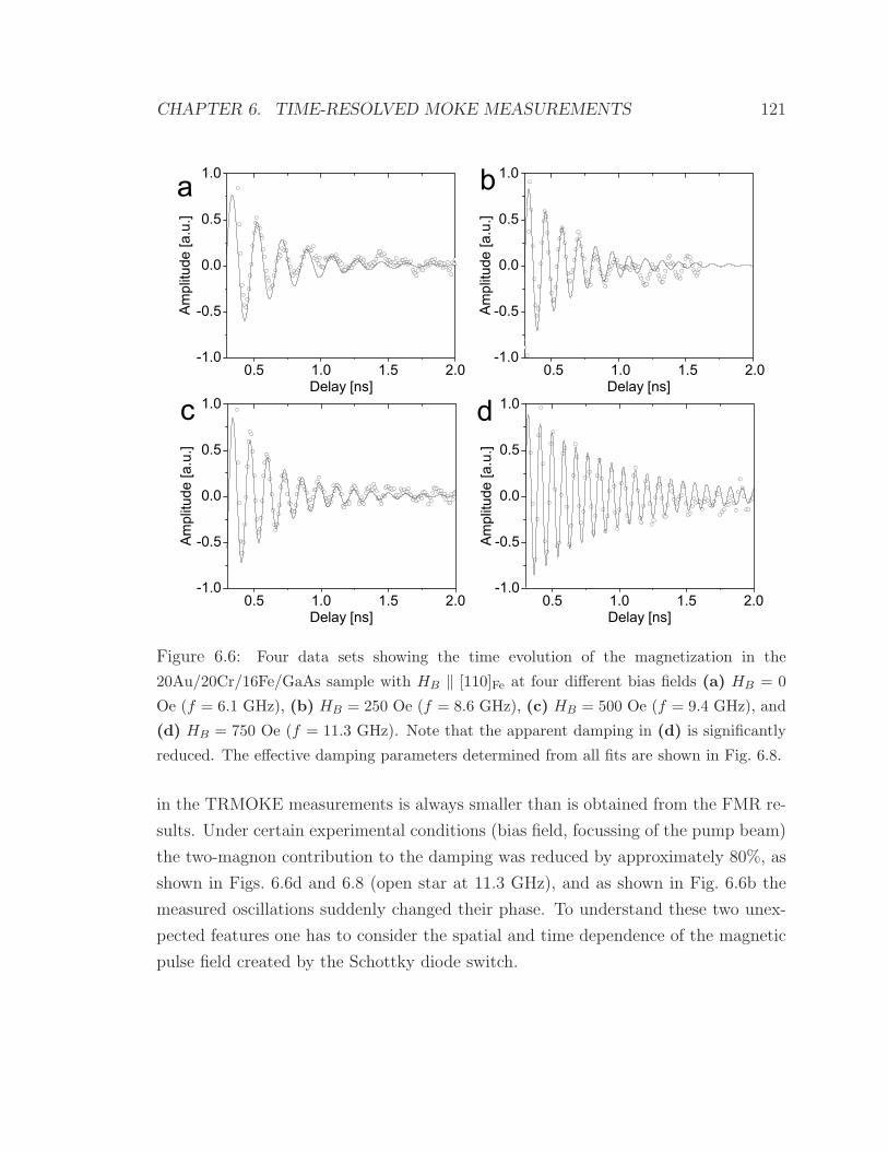
CHAPTER 6. TIME-RESOLVED MOKE MEASUREMENTS 121
Figure 6.6: Four data sets showing the time evolution of the magnetization in the
20Au/20Cr/16Fe/GaAs sample with HB ‖ [110]Fe at four different bias fields (a) HB = 0
Oe (f = 6.1 GHz), (b) HB = 250 Oe (f = 8.6 GHz), (c) HB = 500 Oe (f = 9.4 GHz), and
(d) HB = 750 Oe (f = 11.3 GHz). Note that the apparent damping in (d) is significantly
reduced. The effective damping parameters determined from all fits are shown in Fig. 6.8.
in the TRMOKE measurements is always smaller than is obtained from the FMR re-
sults. Under certain experimental conditions (bias field, focussing of the pump beam)
the two-magnon contribution to the damping was reduced by approximately 80%, as
shown in Figs. 6.6d and 6.8 (open star at 11.3 GHz), and as shown in Fig. 6.6b the
measured oscillations suddenly changed their phase. To understand these two unex-
pected features one has to consider the spatial and time dependence of the magnetic
pulse field created by the Schottky diode switch.

CHAPTER 6. TIME-RESOLVED MOKE MEASUREMENTS 122
6.2.2 Pump field inhomogeneity
µ
Figure 6.7: Cross-section of the
excitation profile generated by
the Schottky diode, where x is
parallel to M.
Since the photo current flows perpendicular to the
Fe/GaAsn interface, its corresponding magnetic field
is oriented in the film plane with circular field lines
centered around the spot of the pump beam, as illus-
trated in Fig. 3.17a. On the circle all angles from 0
to 2π between pump field direction and the direction
of M are realized. The direction of M was fixed by
the bias field to be parallel with [110]Fe. This exci-
tation field configuration is similar to that used in
experiments at SLAC [182, 183] (see also appendix
A). As illustrated in Fig. 3.17a at points, where the
pump field direction is perpendicular to the magnetization the exciting torque reaches
a maximum, and in places where M is parallel or antiparallel to the pump field no
excitation takes place. Since the pump beam and the corresponding photo current
have a Gaussian profile, the field amplitude as a function of distance r from the pump
spot center is given by [87]
h ∼ 1
r
(1 − e−r2/R2
), (6.4)
where R is the radius of the pump spot. The magnetic excitation is sickle shaped on
both sides of the pump spot and is antisymmetric. The spatially most inhomogeneous
Fourier component of the excitation is parallel to M and can be reasonably well
described by a k-vector corresponding to k∗ = 2π/(4R) with k∗ ‖ M, as shown in
Fig. 6.7. This result can be used for the discussion of magnon scattering.
6.2.3 Scattering of inhomogeneous modes
In Fig. 6.9 the spin wave dispersion spectra for in-plane k-vectors were calculated
for f = 6.1 and 11.3 GHz with magnetic parameters corresponding to the 16 ML Fe
film. Based on this figure one can understand why the strength of the two magnon
scattering critically depends on the bias field and the diameter of the laser pump beam
focal spot. At f = 11.3 GHz the excited mode has a k-vector close to the minimum
(bottom) of the spin wave band. In this case there are obviously fewer degenerate
magnons available compared to the lower bias fields where the initial excitation can
find many degenerate spin waves, as illustrated by the intersection of the horizontal

CHAPTER 6. TIME-RESOLVED MOKE MEASUREMENTS 123
α
Figure 6.8: Effective damping parameter as a function of the frequency for the
20Au/20Cr/16Fe/GaAs sample. (•) data points were obtained using FMR [167] and ( )
are the results from the TRMOKE fits. In these experiments the applied field was ‖ [110]Fe.
The () symbols correspond to FMR measurements in the perpendicular configuration and
represent the Gilbert damping.
dotted line with the spin wave manifold in Fig. 6.9. In addition the magnon group
velocity (∂ω/∂k) is zero at the bottom of the spin wave band. These two effects
explain the decreased relaxation which was observed in Figs. 6.6d and 6.8 [184].
The presence of out-of-phase oscillations in Fig. 6.6b might be a consequence of a
mode-mode coupling phenomenon where a significant amount of the initial excitation
scatters into a spin wave mode which is out-of-phase with the initial excitation at the
probed position.
In Fig. 6.8 the relaxation corresponding to this series of measurements was put into
context with the FMR measurements on the same sample [167] (the FMR linewidth
was expressed by an effective damping parameter: αeff = ∆H γω). The effective damp-
ing in the TRMOKE measurements is significantly smaller than that obtained from
FMR at the same frequency (10 GHz). This is probably a consequence of the reduced
number of available spin wave states for scattering in the TRMOKE experiment com-
pared to the FMR experiment, as shown in Fig. 6.9.
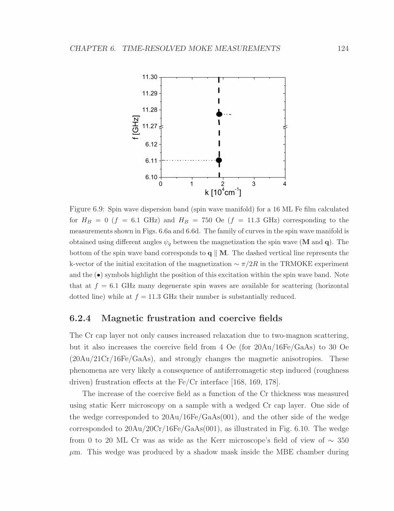
CHAPTER 6. TIME-RESOLVED MOKE MEASUREMENTS 124
Figure 6.9: Spin wave dispersion band (spin wave manifold) for a 16 ML Fe film calculated
for HB = 0 (f = 6.1 GHz) and HB = 750 Oe (f = 11.3 GHz) corresponding to the
measurements shown in Figs. 6.6a and 6.6d. The family of curves in the spin wave manifold is
obtained using different angles ψq between the magnetization the spin wave (M and q). The
bottom of the spin wave band corresponds to q ‖ M. The dashed vertical line represents the
k-vector of the initial excitation of the magnetization ∼ π/2R in the TRMOKE experiment
and the (•) symbols highlight the position of this excitation within the spin wave band. Note
that at f = 6.1 GHz many degenerate spin waves are available for scattering (horizontal
dotted line) while at f = 11.3 GHz their number is substantially reduced.
6.2.4 Magnetic frustration and coercive fields
The Cr cap layer not only causes increased relaxation due to two-magnon scattering,
but it also increases the coercive field from 4 Oe (for 20Au/16Fe/GaAs) to 30 Oe
(20Au/21Cr/16Fe/GaAs), and strongly changes the magnetic anisotropies. These
phenomena are very likely a consequence of antiferromagetic step induced (roughness
driven) frustration effects at the Fe/Cr interface [168, 169, 178].
The increase of the coercive field as a function of the Cr thickness was measured
using static Kerr microscopy on a sample with a wedged Cr cap layer. One side of
the wedge corresponded to 20Au/16Fe/GaAs(001), and the other side of the wedge
corresponded to 20Au/20Cr/16Fe/GaAs(001), as illustrated in Fig. 6.10. The wedge
from 0 to 20 ML Cr was as wide as the Kerr microscope’s field of view of ∼ 350
µm. This wedge was produced by a shadow mask inside the MBE chamber during

CHAPTER 6. TIME-RESOLVED MOKE MEASUREMENTS 125
0 5 10 15 200
50
100
150
200
250
300
350
Pos
ition
[m]
Cr thickness [ML]0 5 10 15 20
0
5
10
15
20
25
30
35
HC
[Oe]
Cr thickness [ML]
4 Oe 6.8 Oe 9.6 Oe 13 Oe 18 Oe 22 Oe 26.3 Oe 27.5 Oe
GaAs(001)
16Fe20Au 20Cr
350 m
H350
m
b c
a
Figure 6.10: (a) Shows a series of domain images (200 µm×350 µm) for a wedged 20Au/0-
20Cr/16Fe/GaAs(001) sample. The black and white arrows indicate the magnetic domains
and the arrow on the right shows the direction of the applied field. (b) Sample reflectivity
and the corresponding thickness of the Cr wedge across the vertical direction of the images.
(c) The coercive fields as a function of the Cr thickness deduced from the series of domain
images in (a) along with a cartoon of the wedged sample.
the growth of the Cr layer. The Cr thickness as a function of the position was
obtained from the changing sample reflectivity (assuming a linear relation between
the reflectivity and the Cr thickness), as can be seen in Fig. 6.10b. A domain wall was
injected from the 20Au/16Fe/GaAs(001) side into the wedge. 20Au/16Fe/GaAs(001)
samples have small coercive fields and the domain walls can be easily controlled in
the field of view of the Kerr microscope by means of an external magnetic field. The
injected domain wall had a zig-zag configuration (head-on) because the slope of the
wedge was parallel to the easy axis of the film ([110]Fe). This wall was driven into the
Cr covered part of the sample and the position of the domain wall was measured as
a function of the applied magnetic pressure. This procedure allowed one to infer the
coercive field as a function of the Cr cap layer thickness (shown in Fig. 6.10c). From
this experiment one can conclude that the increase of the coercive field due to the Cr
cap layer saturates at a thickness of 7 ML of Cr.

CHAPTER 6. TIME-RESOLVED MOKE MEASUREMENTS 126
6.2.5 Field dependent magnetic properties
The measurement of the resonance frequency as a function of the bias field, shown in
Fig. 6.5, directly illustrates how profoundly the magnetic parameters of the 16Fe layer
are affected by the Cr cap layer. Two samples are shown: 20Au/16Fe/GaAsn (•)and 20Au/20Cr/16Fe/GaAsn ( ). Both samples were grown on the same substrate
using a shadow mask inside the MBE chamber. One can therefore attribute the
difference in magnetic properties directly to the different cap layers. In the case of
the Cr cap, the g-factor that describes the data well has the unreasonable value:
g = 1.79, and is at variance with the FMR results obtained at higher frequencies
[167], as shown in Fig. 6.5. This implies that the Cr cap layer gives rise to field or
frequency dependent magnetic anisotropies.
6.3 Single layer measurements in Edmonton
Using the experimental TRMOKE setup in Edmonton, the experiments were repeated
with a transmission line to excite the magnetic film (see details in section 3.3.2). The
magnetic field pulse was delivered using a slotline tapered down to a gap of 10 µm (see
Fig. 3.17b). A GaAs based photo conductive switch generated the ps current pulses.
Compared to the Schottky diode driving used in the Regensburg experiments this
represents a more homogeneous excitation profile having an excitation wavelength of
the order of 10 µm. This method of excitation is more versatile than the Regensburg
technique since it does not require optical transparency of the magnetic film or a
Schottky barrier. A disadvantage, however, is the impedance mismatch between the
transmission line and the photoconductive switch which leads to a partial reflection
of the pump pulse which returns to the sample many several times and effectively re-
excites the sample during the free precession. As a result these pulse reflections have
to be considered in the analysis of the data. Fig. 6.11 shows typical data obtained with
this setup. The presence of pulse reflections is evident in the jumps occurring every
370 ps (indicated by the arrows). The data were analyzed using numerical LLG simu-
lations which include the presence of the reflected pulses. The actual magnetic pulse
shape (including the pulse reflections) was obtained from the quasi magneto-static re-
sponse of the sample. The quasi magneto-static response was measured by applying
the highest possible bias field (4 kOe) and filtering the resulting TRMOKE data with
a running average window (see solid line in Fig. 6.11a). For the 20Au/16Fe/GaAs

CHAPTER 6. TIME-RESOLVED MOKE MEASUREMENTS 127
Figure 6.11: TRMOKE measurements using a stripline for (a) 20Au/16Fe/GaAs in the
presence of a bias field HB = 1 kOe (f = 15.2 GHz) and (b) 20Au/21Cr/16Fe/GaAs with
HB = 1.2 kOe (f = 14.0 GHz). In each case HB was applied along the [110]Fe direction.
The solid line is a numeric fit using the LLG equation which takes the reflections of the
pump pulse into account. The magnetic parameters used for the calculation are shown in
Fig. 4.5 for (a) and listed in [167] for (b). In (a) the excitation field shape used for the fits
is shown in the thick solid line. This shape was obtained by filtering TRMOKE data which
were measured with a higher bias field (see explanation in the text). The vertical arrows
indicate the times at which the the pump pulse reflections were incident on the specimen.
The inset in (a) has an expanded time scale to demonstrate the quality of the fit.
sample this analysis resulted in the damping constant α = 3.7± 0.1× 10⁻³. This is in
agreement with the damping parameter observed in FMR and 10% bigger than that
measured using the TRMOKE setup in Regensburg. In the 20Au/20Cr/16Fe/GaAs
sample the damping parameter was found to be α = 1.8 ± 0.1 × 10⁻² and again 30%
smaller compared to the value obtained using FMR at the same frequency, as shown
in Fig. 6.8.
Since easy and hard directions of the magnetic anisotropies are known, the pre-
cessional frequency as a function of the bias field along easy [110]Fe and hard [110]Fe
directions can be used to determine not only g and 4πMeff , but also the magnetic
in-plane anisotropies K‖1 and K
‖U , by comparing the data with calculations. The fre-
quency dependence for fields applied in directions close to the [110]Fe axis was already
calculated for this sample in a previous section (Fig. 4.8) where the presence of K‖1
and K‖U leads to 3 separate FMR peaks with increasing applied field at 9.5 GHz. If
HB is applied close to the hard magnetic axis the magnetization rotates from the
[110]Fe direction to the [110]Fe direction as the field is increased from HB = 0. The

CHAPTER 6. TIME-RESOLVED MOKE MEASUREMENTS 128
Figure 6.12: Frequency vs. bias field for the 20Au/16Fe/GaAs sample. (•) symbols were
obtained with HB ‖ [110]Fe and () symbols correspond to HB ‖ [110]Fe. The solid lines were
calculated using the following parameters: 4πMeff = 17.0 kOe, g = 2.09, K‖1 = 2.5 × 10⁵
erg/cm3, and K‖U = −5.4× 10⁵ erg/cm3. A misalignment of HB with respect to the [110]Fe
direction of δϕH = 1.15 was used for the calculation of the hard axis curve.
frequency versus bias field curve has a characteristic shape with a maximum and a
minimum when HB is applied close to [110]Fe determined by the size of K‖1 and K
‖U .
The maximum occurs at HB = 2K‖1/MS and the position of the frequency dip is
given by 2(K‖1 −K
‖U)/MS ([110]Fe is the hard direction for both magnetic anisotropies
and KU is negative). The data with HB oriented along the [110]Fe direction shown
in Fig. 6.11 are consistent with an in-plane misalignment of the field of δϕH = 1.15
with respect to the [110]Fe direction. This misalignment is the reason why the preces-
sional frequency does not drop to zero when the anisotropy fields are compensated at
HB = 2(K‖1 − K
‖U)/MS.
6.4 Summary
The dynamic properties of magnetic single layers with Gilbert damping determined
from FMR measurements were well reproduced in TRMOKE experiments. In both
TRMOKE configurations (Schottky diode and transmission line) the magentization
was excited very inhomogeneously. Counil et al. [185] recently addressed the high
frequency response of a spatially inhomogeneously excited magnetic film and found
an appreciable increase in the measured frequency linewidth at low frequencies for a
CHAPTER 6. TIME-RESOLVED MOKE MEASUREMENTS 129
50 nm Permalloy film due to dephasing of the excited spin waves. This effect was
not observed in the samples discussed in this section because the magnetic films were
very thin (∼ 2 nm). In ultrathin films this effect is weaker because the q‖tF term in
Eq. 2.48 is small. In this case the frequency spread of the excited spin wave band is
very narrow (a few MHz) compared to the intrinsic frequency linewidth (∼ 100 MHz)
and does not cause significant dephasing.
In the Cr/Fe/GaAs samples which exhibit a strong two-magnon relaxation, the
dynamic response of these samples was clearly affected by the inhomogeneous excita-
tion. When the wave vector of the initially excited spin wave was close to the bottom
of the spin wave dispersion band the two-magnon relaxation was significantly reduced.

Chapter 7
Conclusions
High quality epitaxial single crystalline Au/Fe/GaAs(001) multilayers having sharp
interfaces were grown by means of molecular beam epitaxy and characterized using
refection high energy electron diffraction (RHEED), scanning tunnelling microscopy
(STM) and cross-sectional transmission electron microscopy (TEM). The magnetic
properties of Au/Fe/GaAs(001) single layers were investigated using ferromagnetic
resonance (FMR). The homogeneity of these ultrathin magnetic films resulted in
nearly ideal behavior (i.e. no extrinsic contributions to the FMR linewidth) and al-
lowed for reproducible studies of the effect of cap layers on the ferromagnetic relax-
ation.
This study led to four important results:
(1) For Au/Fe/Au/Fe/GaAs(001) double layers a large increase in the Gilbert
damping was observed. The additional damping scaled inversely with the Fe film
thickness, i.e. the presence of a second ferromagnetic layer resulted in an additional
interface Gilbert damping. This effect was explained in terms of a spin-pump/spin-
sink model. A crossover of the FMR fields of the two Fe layers allowed this model to be
tested in detail. Theory and experiment were found to be in excellent qualitative and
quantitative agreement. For the first time a spin current was observed in absence of a
charge current. This effect may lead to a new type of electronics which is independent
of electric charge transport.
(2) The spin-sink effect was studied in normal metals (NM) using NM/Fe/-
GaAs(001) samples, where NM=Au, Ag, Cu, and Pd. The Au, Ag, and Cu cap
layers with NM thicknesses of up to 80 nm did not result in a measurable additional
FMR linewidth. This is consistent with the expected large spin diffusion length in
130
CHAPTER 7. CONCLUSIONS 131
Au, Ag, and Cu. Samples with Pd cap layers behaved differently. Pd cap layers above
10 nm acted as a perfect spin-sink with the strength of spin-pumping close to that
expected from the density of free electrons in Pd. Pd is a NM that exhibits strong
spin electron-electron correlations which result in paramagnons. It is argued that the
spin-sink effect in Pd is due to the dissipation of the pumped spin current by the
interaction with spin fluctuations inherent to Pd. The experimental result implies
that the relaxation of spin momentum in Pd occurs in the ballistic limit, that is the
spin mean free path is shorter than the momentum mean free path.
(3) A self organized network of misfit dislocations was identified by RHEED, plan
view TEM, and STM in the lattice strained Pd/Fe/GaAs system. The magnetic
relaxation in such samples increased and was strongly anisotropic; the anisotropy was
observed to exhibit the rectangular symmetry of the misfit dislocation network. It
was shown that this system provides a classical example of two-magnon scattering
and that the angular dependence of the extrinsic relaxation can be explained by the
channelling of scattered spin waves parallel to the misfit dislocations.
(4) A Cr/Fe/GaAs sample was used to test the effect of two-magnon scattering
in the time domain using a time-resolved Kerr effect experiment. For this sample the
effective relaxation constant was strongly dependent on the experimental conditions.
The wave vector of the initial excitation of the magnetization was always constant,
but the wave vector corresponding to the bottom of the spin wave dispersion band
was changed by a variable magnetic bias field. When the wave vectors of the initial
excitation of the magnetization and the bottom of the spin wave dispersion band
coincided the two-magnon contribution to the relaxation was nearly switched off.
This striking result shows that the apparent magnitude of two-magnon scattering
depends on the size of the probe involved in the measurement as well as the wave
vector that is used to excite the magnetization.

Appendix A
SLAC experiment
The dynamic properties of Au/Fe/GaAs(001) magnetic single layers were discussed
in chapters 4 and 6. FMR and TRMOKE however only explore the dynamics in the
limit of small precessional angles. For many device applications it is important to
understand the magnetic relaxation at large precessional angles. The Au/Fe/GaAs
magnetic single layer samples described in section 4.2 with their well defined intrinsic
properties provide a model case. The generation of short magnetic field pulses strong
enough to incline the magnetization in the Au/Fe/GaAs(001) samples by appreciable
angle is a major challenge.
Siegmann et al. [182, 186, 183] have demonstrated the possibility of using a pulsed
and focused 50 GeV electron beam in the Final Focus Test Beam (FFTB) section of
the Stanford Linear Accelerator Center (SLAC) as magnetic field source. This electron
beam was focussed to micrometer dimensions and provides field pulses of up to 200
kOe with 1-8 ps duration.
These are the strongest magnetic field pulses known. The principle of this exper-
iment is illustrated in Fig. A.1. The in-plane magnetic field pulse tilts the magnetiza-
tion instantaneously out of the plane and the relaxation proceeds by free precession. If
the out-of-plane tilt angle exceeds 12 for a 10Au/15Fe/GaAs(001) sample, then the
magnetization precesses at a very large cone angle (∼ 78) as illustrated in Fig. A.2
in the resulting demagnetizing field. The number of large angle precessions and hence
the final direction of the magnetization is determined by the size of the initial tilt
angle.
The initial tilt angle depends on the size of torque T = M × h exerted by the
pulse magnetic field pulse h. Since h is a circular field, and falls of as 1/r from the
132

APPENDIX A. SLAC EXPERIMENT 133
Figure A.1: Cartoon of the experimental configuration of the SLAC experiment.
Figure A.2: 3D trajectory of the magentization in the 10Au/15Fe/GaAs(001) sample.
The magnetization (big arrow) was initially oriented parallel to [110]Fe. In this example
the magnetization is tilted out of the plane by 12.5 (dotted arrow) and precesses freely in
demagnetizing and anisotropy fields (switching twice) before settling in the [110]Fe direction.
center of the electron beam the resulting domain configuration consists of ∞ shaped
contours each given by a nearly constant initial tilt angle.

APPENDIX A. SLAC EXPERIMENT 134
300 m M
Figure A.3: Domain pattern written by a SLAC pulse into a uniaxial 10Au/15Fe/GaAs
sample. The pattern was imaged by SEMPA. The background shows a calculated mangeti-
zation pattern using the LLG equation using magnetic properties consistent with FMR, see
Fig. 4.5a, a damping coefficient α = 0.017, and pulse amplitude and duration as determined
during the exposure.
A.1 Results
In collaboration with Professor Hans Siegmann experiments with the SLAC electron
pulses were performed with Au/Fe/GaAs(001) samples [187]. Fig. A.3 shows a switch-
ing pattern that was produced in a 10Au/15Fe/GaAs(001) sample by exposing it to a
single Gaussian electron pulse of width τ = 2.3 ps. Prior to the arrival of the electron
bunch, the film was magnetized along its easy direction ([110]Fe), as indicated by the
arrow labelled M. Subsequently, the Au cap layer was removed by sputtering, and
the pattern was imaged with a scanning electron microscope with polarization anal-
ysis (SEMPA). The dark regions are locations where the magnetization has switched
into the opposite direction while the light grey regions are the locations were the
direction of M either remained unchanged, or switched back to the initial direction
after multiple reversals. The switching pattern due to the focussed electron bunch
extends to large distances (in Fig. A.3 up to 300 µm) from the center of the electron
beam. A circular damaged area appears around the place where the electron bunch
has passed. It is very likely caused by damage in the GaAs(001) substrate due to
the electric field accompanying the electron bunch. In GaAs the E-field cannot be

APPENDIX A. SLAC EXPERIMENT 135
screened on a ultrafast time scale and may produce cracks or other damage in the
ionic semiconductor crystal.
The gross features of the resulting magnetization pattern shown in Fig. A.3 can
be explained by uniform precession of the magnetization [188]. Specifically, the figure
8-shape of the pattern reflects the lines of constant precessional torque T = M × h.
Up to 10 switches of the magnetization back and forth can be distinguished as one
moves closer to the center of the electron beam. The calculated pattern in Fig. A.3
that fits the data allows one to determine anisotropies and damping constant. The
magnetic anisotropies obtained from the pattern agree with the FMR results in 4.5a.
On the other hand, the damping constant was found to be α = 0.017 and hence 4
times larger than in FMR.
A.2 Discussion
Domain wall mobility measurements allow one to estimate the damping for 180 pre-
cession since the magnetic damping exerts a viscous force on a moving wall [9]. Leaver
and Vojndani [189] measured the domain wall mobility in Ni at 1 MHz. Their mobil-
ity is agreement with intrinsic damping for Ni measured by FMR [131]. Nibarger et
al. [190] recently measured damping constant as a function of the precessional angle
from 0 up to 40 and found the damping to be independent on the precessional cone
angle.
The crucial difference between these experiments and the SLAC experiment is the
precessional frequency. Nibarger et al. were only able to reach a precessional angle
of 40 at frequencies as low as 400 MHz. In the SLAC experiment the free precession
occurs at almost 8 GHz.
A.3 Multi-magnon scattering
Recently, Dobin et al. [191] addressed large angle precession at high frequencies (fields)
from a theoretical point of view. It was found that intrinsic three and four-magnon
processes, which are similar to Suhl instabilities at high microwave power levels [192],
can contribute to the relaxation rate of the magnetization. For a Fe film of 2 nm
thickness with a bias field of 1 kOe at a precessional cone angle of 45, they find a
relaxation time of 0.3 ns corresponding to α = 0.019 (see Fig. 3 in [191]). These con-

APPENDIX A. SLAC EXPERIMENT 136
ditions are actually very close to the SLAC experiment since the 10Au/15Fe/GaAs
and 10Au/10Fe/GaAs samples have effective bias fields of 500 and 800 Oe built-in
(due to anisotropies). According to Dobin el al. [191] the magnon scattering effects
are smaller for smaller applied fields, because the size of the k-space of initially de-
generate magnons (shown in Fig. 5.11) decreases. This model therefore does not
necessarily contradict the experiments by Nibarger et al. [190] and Leaver and Vojn-
dani [189]. In these experiments the magnon processes were not operative since the
fields (frequencies) were very small.
If multi-magnon scattering is responsible for the perceived increase in magnetic
damping is remarkable that a well defined switching pattern appears. According to
Dobin et al. the effective magnetization reduces by ∼ 40% during the precession due
to the generation of spin waves with k = 0. It is remarkable that this does not lead
to chaos in the resulting switching pattern.
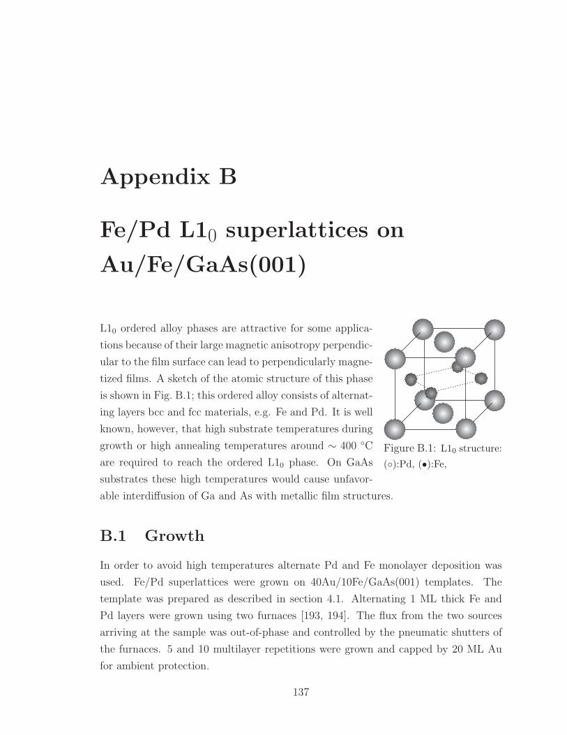
Appendix B
Fe/Pd L10 superlattices on
Au/Fe/GaAs(001)
Figure B.1: L10 structure:
():Pd, (•):Fe,
L10 ordered alloy phases are attractive for some applica-
tions because of their large magnetic anisotropy perpendic-
ular to the film surface can lead to perpendicularly magne-
tized films. A sketch of the atomic structure of this phase
is shown in Fig. B.1; this ordered alloy consists of alternat-
ing layers bcc and fcc materials, e.g. Fe and Pd. It is well
known, however, that high substrate temperatures during
growth or high annealing temperatures around ∼ 400 C
are required to reach the ordered L10 phase. On GaAs
substrates these high temperatures would cause unfavor-
able interdiffusion of Ga and As with metallic film structures.
B.1 Growth
In order to avoid high temperatures alternate Pd and Fe monolayer deposition was
used. Fe/Pd superlattices were grown on 40Au/10Fe/GaAs(001) templates. The
template was prepared as described in section 4.1. Alternating 1 ML thick Fe and
Pd layers were grown using two furnaces [193, 194]. The flux from the two sources
arriving at the sample was out-of-phase and controlled by the pneumatic shutters of
the furnaces. 5 and 10 multilayer repetitions were grown and capped by 20 ML Au
for ambient protection.
137
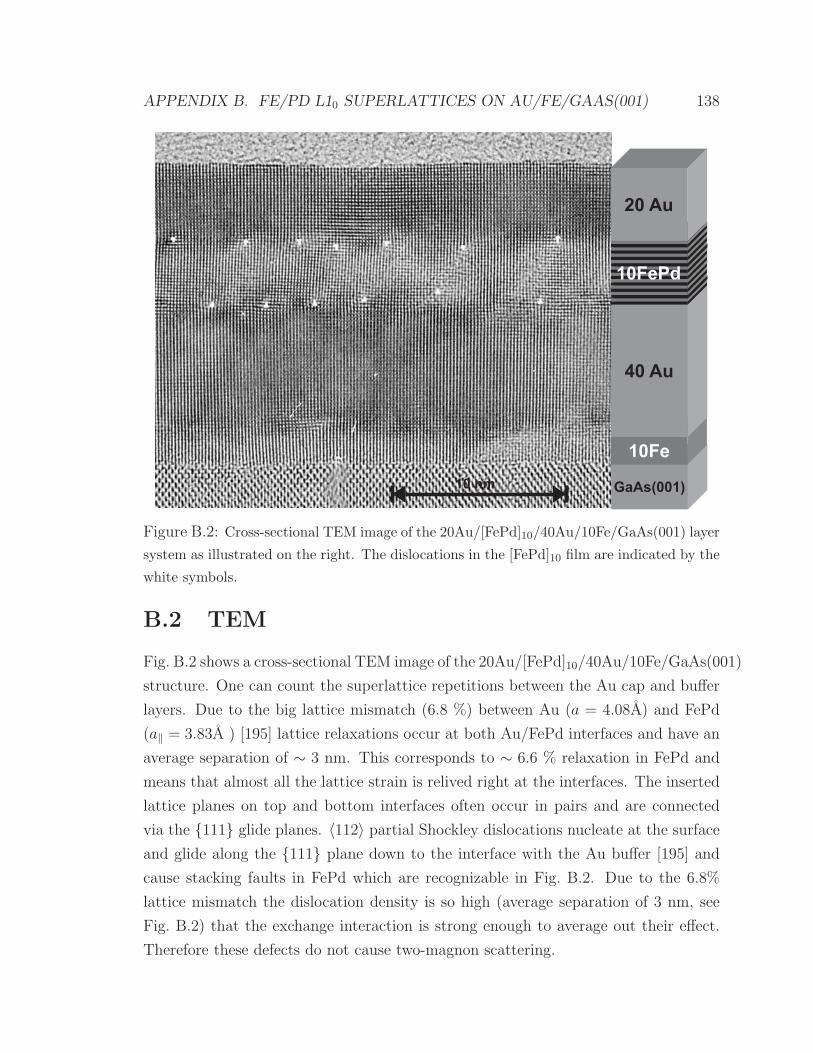
APPENDIX B. FE/PD L10 SUPERLATTICES ON AU/FE/GAAS(001) 138
GaAs(001)
10Fe
40 Au
20 Au
10FePd
10 nm
Figure B.2: Cross-sectional TEM image of the 20Au/[FePd]10/40Au/10Fe/GaAs(001) layer
system as illustrated on the right. The dislocations in the [FePd]10 film are indicated by the
white symbols.
B.2 TEM
Fig. B.2 shows a cross-sectional TEM image of the 20Au/[FePd]10/40Au/10Fe/GaAs(001)
structure. One can count the superlattice repetitions between the Au cap and buffer
layers. Due to the big lattice mismatch (6.8 %) between Au (a = 4.08A) and FePd
(a‖ = 3.83A ) [195] lattice relaxations occur at both Au/FePd interfaces and have an
average separation of ∼ 3 nm. This corresponds to ∼ 6.6 % relaxation in FePd and
means that almost all the lattice strain is relived right at the interfaces. The inserted
lattice planes on top and bottom interfaces often occur in pairs and are connected
via the 111 glide planes. 〈112〉 partial Shockley dislocations nucleate at the surface
and glide along the 111 plane down to the interface with the Au buffer [195] and
cause stacking faults in FePd which are recognizable in Fig. B.2. Due to the 6.8%
lattice mismatch the dislocation density is so high (average separation of 3 nm, see
Fig. B.2) that the exchange interaction is strong enough to average out their effect.
Therefore these defects do not cause two-magnon scattering.

APPENDIX B. FE/PD L10 SUPERLATTICES ON AU/FE/GAAS(001) 139
χµ
Θ
Figure B.3: (a) The left figure shows a FMR spectrum of the 20Au/[FePd]-
10/40Au/10Fe/GaAs(001) sample. () symbols correspond to the measurement and the solid
line is a calculated FMR spectrum for the bilayer system including all magnetic anisotropies.
Note that the slight asymmetry of the data was caused by the microwave cavity. (b) Θ−2Θ
x-ray diffraction scan of the 20Au/[FePd]10/40Au/10Fe/GaAs(001) sample. The wavelength
was λ = 1.54A (CuKα). Due to the finite crystal thickness the multilayer peaks are intrin-
sically broadened; e.g. the intrinsic broadening of a 20 ML Au film results in ∆2Θ = 4 and
∆2Θ = 8 for the Au(002) and Au(004) peaks, respectively.
B.3 FMR
The FMR spectra of the FePd layer were given by narrow Lorentzian lines. The
magnetic in-plane anisotropies observed in FMR were extremely weak. From the
linear frequency dependence of the FMR linewidth with no zero frequency offset one
can conclude that the damping is only intrinsic and enhanced by the spin pumping
contribution due to vicinity of the 10 Fe seed layer. For the [FePd]10 layer the following
magnetic parameters were found: 4πMeff = 10.1 kG, K‖U = −1 × 10⁵ erg/cm3, and
K‖1 = 0.
By direct comparison of the FMR peaks of the 10Fe layer and the [FePd]10 layer
one can determine the magnetic moment of [FePd]10. The moment was estimated by
superimposing calculated and measured FMR lines (see Fig. B.3). Because the 10Fe
layer has a known magnetic moment, the moment of the [FePd]10 layer was adjusted
to get the best fit. This procedure resulted in MFePdS = 1180± 60 emu/cm3, which is
in very good agreement with other values reported for FePd [196, 197].
First principles calculations for the FePd structure by Stoeffler [198] indicate that

APPENDIX B. FE/PD L10 SUPERLATTICES ON AU/FE/GAAS(001) 140
the magnetic moment per Pd atom should be 0.3 µB. If one correlates this with
the measured saturation magnetization this results in a strongly enhanced magnetic
moment for Fe 3.0 ± 0.1 µB. This enhancement was also predicted and is related to
the atomic volume increase for Fe in the L10 structure. Similar enhancements were
reported for Fe in other L10 structures [199].
Since 4πMeff was nearly independent of the thickness of the superlattice the dif-
ference between 4πMeff and 4πMS is a bulk effect with K⊥U = 3 × 10⁶ erg/cm3. This
perpendicular uniaxial anisotropy is much weaker than it should be for the well or-
dered L10 phase [200]. Gehanno et al. [197] obtained a 5 times larger value for K⊥U
in FePd(001) films deposited at 300 C on MgO(001).
One can get an estimate of the order in the FePd superlattice from out-of-plane
x-ray diffraction (XRD) measurements. Wide angle radial scans across the recipro-
cal lattice normal to the growth direction provide information about the structural
coherence.
The one dimensional chemical order parameter S is defined as [201]
S =rFe − xFe
yPd
=rPd − xPd
yFe
, (B.1)
where xFe(Pd) = 12
is the atomic fraction of Fe(Pd) in the sample, yFe(Pd) = 12
is the
fraction of Fe(Pd) atomic sites, and rFe(Pd) is the fraction of Fe(Pd) sites occupied by
the correct species. S = 1 for a perfectly ordered film of stoichiometric composition
Fe50Pd50. In x-ray diffraction (XRD) this order parameter can be related to the
relative ratio of the FePd fundamental (002) peak and the satellites peaks FePd(001)
and FePd(003). One can write [194]
S2 =[IFePd(002)/IFePd(003)]observed
[IFePd(002)/IFePd(003)]S=1calculated
. (B.2)
Fig. B.3b shows a θ − 2θ scan of the 20Au/[FePd]5/40Au/10Fe/GaAs(001) sample.
One can recognize peaks corresponding to GaAs, Au, and FePd. The measured ratio
between FePd(002) and FePd(003) leads to S = 0.4 ± 0.2 (using IFePd(003)/IFePd(002)
calculated for S = 1 for the FePt structure [193]).
B.4 Conclusion
Well ordered FePd superlattices with perpendicular magnetization cannot be prepared
at RT even by monolayer modulated MBE. The L10 phase is preferred only at high

APPENDIX B. FE/PD L10 SUPERLATTICES ON AU/FE/GAAS(001) 141
temperatures and the disorder from low temperature preparation results in a per-
pendicular anisotropy that is too small to compensate the demagnetizing field. This
is a general behavior of the L10 phase and in agreement with results found for other
L10 superlattices [193, 194, 201]. A feature the 20Au/[FePd]n/40Au/10Fe/GaAs(001)
bilayer system that may be useful for spintronics applications is that both magnetic
layers are uniaxial with their easy axes parallel to each other and along the [110]Fe
direction.

Appendix C
Theory of Spin-Pumping
At this time there is no citable reference detailing the justification of the spin-
pumping theory. The following derivation of the spin-pumping theory as introduced
by Tserkovnyak et al. [116] is based on lecture notes provided by Prof. Evgen Simanek.
C.1 Diagonalization of the Hamiltonian
M
x
y
z
θ
φ
Figure C.1: Coordinate system
The Hamiltonian of conduction electrons in the laboratory system is given by
H =
[−
2m∇2 + V n(r)
]1 + (σ · m)V s(r) (C.1)
where V n(r) is the spin-independent and V s(r) is the spin-dependent (exchange)
142

APPENDIX C. THEORY OF SPIN-PUMPING 143
potential. The unit and Pauli matrices are
1 =
(1 0
0 1
), σx =
(0 1
1 0
), σy =
(0 −1
−1 0
), σz =
(1 0
0 −1
), (C.2)
and the unit vector of the magnetization is
m =M
Ms
=
sin θ cos φ
sin θ sin φ
cos θ
, (C.3)
where θ and φ are cone and phase angle of m respectively. In order to diagonalize H
a unitary matrix that rotates the z-axis parallel to m is defined
U =
(cos ( θ
2)e−i φ
2 − sin ( θ2)e−i φ
2
sin θ2ei φ
2 cos θ2ei φ
2
)(C.4)
with the inverse
U−1 =
(cos θ
2ei φ
2 sin θ2e−i φ
2
− sin θ2ei φ
2 cos θ2e−i φ
2
). (C.5)
The Schrodinger equation (SE) in the laboratory system is given by
HΨ = EΨ, (C.6)
where Ψ is a spinor. After a rotation about z
Ψ = UΦ, and HU = U−1HU (C.7)
one obtains the SE in the rotated System
HU Φ = EΦ. (C.8)
Diagonalizing the exchange part of H from C.3 one has
σ · m =
(cos θ sin θe−i φ
sin θeiφ − cos θ
)(C.9)
Using C.4, C.5, and C.9 it follows that
U−1σ · mU =
(1 0
0 −1
)= σz. (C.10)

APPENDIX C. THEORY OF SPIN-PUMPING 144
The resulting Hamiltonian in the rotated system is thus diagonal in the spin (s = 1/2)
space of the conduction electrons:
HU =
[−
2m∇2 + V n(r)
]1 + σzV
s(r). (C.11)
The spinor transformation in components (s = ±1/2) is:
Ψs = UsσΦσ, (C.12)
where
Φ↑ = Φ(r)
(1
0
), Φ↓ = Φ(r)
(0
1
). (C.13)
C.2 Reflection matrix
ms′ ns
t′
r
ns
ms′
NF
Figure C.2: Cartoon illustrating the meaning of the F/N interface scattering coeffi-
cients.
The reflection matrix is defined as
Ψns =
∑m,s′
χm(ρ)√km
[δss′δnmξs′e
iknx + rnmss′ ξs′e
−ikmx], (C.14)

APPENDIX C. THEORY OF SPIN-PUMPING 145
where the χ(ρ) = χ(y, z) are the transverse modes. In the rotated system Eq. C.14
reads
Φnr =
∑m,s′
χm(ρ′)√km
[δrs′δnmξU,s′e
iknx + rnmU,rs′ ξU,s′e
−ikmx]. (C.15)
From C.12, C.14, and C.15 it follows
rss′ = (U rU U−1)ss′ . (C.16)
Proof of C.16: Since C.15 is a solution in the rotated (diagonalized) system (see C.11),
the spinor
ξU,↑ =
(1
0
)and ξU,↓ =
(0
1
)(C.17)
According to C.12, the spinor ξs′ (in C.14) in the laboratory system is
ξs′ = Us′σ ξU,σ. (C.18)
Inserting C.18 into C.14 results in
Ψns =
∑m,s′
χm(ρ)√km
[δss′δnmUs′σ ξU,σe
iknx + rnmss′ Us′σ ξU,σe
−ikmx]. (C.19)
Multiplying C.15 on the left by the matrix Usr and using C.12 yields
Ψns = UsγΦ
nr =
∑m,s′
χm(ρ)√km
[Usγδrs′δnmξU,s′e
iknx + UsrrnmU,γs′ ξU,s′e
−ikmx]. (C.20)
The reflection terms of C.19 and C.20 should be equal to each other. This implies
(dropping m,n indices):
rss′Us′σ ξU,σ = Usγ rU,γs′ ξU,s =let s′→σ Usγ rU,γσ ξU,σ (C.21)
Equation C.21 implies
rss′Us′σ = Usγ rU,γσ. (C.22)
Multiplying C.22 on the right by U−1σδ and summing over σ results in
rss′Us′σU−1σδ = Usγ rU,γσU
−1σδ . (C.23)

APPENDIX C. THEORY OF SPIN-PUMPING 146
But U U−1 = 1, so that
Us′σU−1σδ = δs′,δ. (C.24)
Using C.24 in C.23, one obtains
rsδ =(U rU U−1
)sδ
, (C.25)
which proves relation C.16.
Since U is a function of the θ and φ angles of M relation C.16 allows one to
calculate the effect of precession of the magnetization on rsσ(≡reflection matrix in
laboratory system) from the knowledge of rU(≡reflection matrix in system where
m ‖ z).
C.3 Reflection without spin-flip (rotated system)
Assume
rU,ss′ = δss′ rU,ss, (C.26)
this gives (U rU U−1
)ss′
= UsσrU,σσ′U−1σ′s′
= UsσrU,σσU−1σs′ (C.27)
= Us↑U−1↑s′ rU,↑↑ + Us↓U−1
↓s′ rU,↓↓.
Now one can evaluate the matrix element Us↑U−1↑s′ from:
U =
(U↑↑ U↑↓U↓↑ U↓↓
)=
(cos θ
2e−i φ
2 − sin θ2e−i φ
2
sin θ2ei φ
2 cos θ2ei φ
2
)and
U−1 =
(U−1↑↑ U−1
↑↓U−1↓↑ U−1
↓↓
)=
(cos θ
2ei φ
2 sin θ2e−i φ
2
− sin θ2ei φ
2 cos θ2e−i φ
2
), (C.28)
hence
U↑↑U−1↑↑ = cos2 θ
2
U↑↑U−1↑↓ = cos
θ
2sin
θ
2e−iφ (C.29)
U↑↑U−1↑↑ = cos
θ
2sin
θ
2eiφ
U↓↑U−1↑↓ = sin2 θ
2,

APPENDIX C. THEORY OF SPIN-PUMPING 147
this determines
Us↑U−1↑s′ =
(cos2 θ
2cos θ
2sin θ
2e−iφ
cos θ2sin θ
2eiφ sin2 θ
2
)s,s′
and (C.30)
Us↓U−1↓s′ =
(sin2 θ
2− sin θ
2cos θ
2e−iφ
− sin θ2cos θ
2eiφ cos2 θ
2
)s,s′
. (C.31)
Eqs. C.30 and C.31 can be expressed more compactly as
Us↑U−1↑s′ =
1
2
(1 + σ · m
)s,s′
(C.32)
Us↓U−1↓s′ =
1
2
(1 − σ · m
)s,s′
. (C.33)
C.4 Spin projection operators
Define
u(+) =1
2
(1 + σ · m
)(C.34)
u(−) =1
2
(1 − σ · m
). (C.35)
The operator σ · m has the property(σ · m
)2
= 1 (C.36)
because the Pauli matrices fulfill the following theorem:(σ · A
)(σ · B
)=(
A · B)
1 + iσ ·(
A × B)
(C.37)
and by setting A = B = m and noting |m| = 1. This implies that u(+) and u(−) are
projection operators. In order to consider their projection properties the state vector
is defined as
ψ =
(ψ↑ψ↓
). (C.38)
Then define
ψ(+) = u(+)ψ (C.39)
ψ(−) = u(−)ψ. (C.40)

APPENDIX C. THEORY OF SPIN-PUMPING 148
Using C.33 in C.39 one finds the explicit form of the vector ψ(+):
u(+)ψ =
(12(1 + cos θ) 1
2sin θe−iφ
12sin θeiφ 1
2(1 − cos θ)
)(ψ↑ψ↓
). (C.41)
Eqs. C.39 and C.41 imply
ψ(+) =
(ψ
(+)↑
ψ(+)↑
)=
(12(1 + cos θ)ψ↑ 1
2sin θe−iφψ↑
12sin θeiφψ↓ 1
2(1 − cos θ)ψ↓
). (C.42)
Multiplication of C.39 on the left by σ · m and using C.36 yields(σ · m
)ψ(+) =
(σ · m
) 1
2
(1 + σ · m
)ψ =
1
2
(σ · m + 1
)ψ = ψ(+). (C.43)
Hence ψ(+) is an eigenvector of(σ · m
)with eigenvalue +1. Similarly
(σ · m
)ψ(−) = −ψ(−), (C.44)
i.e. ψ(−) is an eigenvector of(σ · m
)with eigenvalue −1. Note that the projection
properties of u(+) and u(−) are a consequence of identity C.36. This result is valid for
any operator. u(+) and u(−) are called spin projection matrices.
C.5 Transmission matrix (laboratory system)
The outgoing wave in the laboratory system Ψns is defined as
Ψns =
∑m,s′
χm(ρ)√km
tnmss′ ξs′e
ikmx, (C.45)
while the outgoing wave in the rotated system is Φns
Φns =
∑m,s′
χm(ρ)√km
tnmU,ss′ ξU,s′e
ikmx. (C.46)
The spinor ξs′ satisfies C.18. Since the RHS of C.45 and C.46 has a form similar to
C.14 and C.15, respectively, one can follow steps C.19-C.25, and show
tss′ = (U tU U−1)ss′ . (C.47)

APPENDIX C. THEORY OF SPIN-PUMPING 149
Hence the transformation laws for t and r are the same (see C.16). Now consider
electron transmission without spin-flip (in the rotated system). Assume
tU,ss′ = δs,s′ tU,ss. (C.48)
Similar to C.27 one can deduce from C.48(U tU U−1
)ss′
= Us↑U−1↑s′ tU,↑↑ + Us↓U−1
↓s′ tU,↓↓. (C.49)
From Eqs. C.16, C.27, C.32, C.33, C.47, and C.49 one can determine the transforma-
tion for the reflection and transmission matrices:
rmn = rmnU,↑↑u
(+) + rmnU,↓↓u
(−) (C.50)
tmn = tmnU,↑↑u
(+) + tmnU,↓↓u
(−). (C.51)
Although the rU and tU matrices are diagonal in spin space, the r and t matrices are
not (due to the spin projection operators u(+) and u(−)). This means even without
spin-flip in the rotated system there is spin-flip in the laboratory system.
C.6 The scattering matrix for the N/F/N-sandwich
Now the scattering due to a ferromagnetic layer (F) inserted between two normal metal
(N) layers will be treated. Left and right N layer will be called L and R respectively.
The scattering matrix in (L,R) is defined by
S =
(SRR SRL
SLR SLL
)=
(r t
t′ r′
)=
(r t
t r
), (C.52)
where the third equality is due to symmetry; L and R are assumed to be identical
paramagnets meaning t′ = t and r = r′.
One needs to perform the transformation of S from the laboratory system into
the rotated system. Using C.51 one has (skipping n,m labels)
S =
(rmnU,↑↑u
(+) + rmnU,↓↓u
(−) tmnU,↑↑u
(+) + tmnU,↓↓u
(−)
tmnU,↑↑u
(+) + tmnU,↓↓u
(−) rmnU,↑↑u
(+) + rmnU,↓↓u
(−)
)= SU,↑↑u(+) + SU,↓↓u(−), (C.53)
where
SU,↑↑ =
(rU,↑↑ tU,↑↑tU,↑↑ rU,↑↑
)and SU,↓↓ =
(rU,↓↓ tU,↓↓tU,↓↓ rU,↓↓
). (C.54)

APPENDIX C. THEORY OF SPIN-PUMPING 150
C.7 Current induced by modulation of the chemi-
cal potential
The theory of Tserkovnyak et al. [116] is based on the following equation:
Ipump(t) = e∂n(l)
∂X
dX(t)
dt, (C.55)
where Ipump is the matrix current (2 × 2 matrix in s=12
space), X(t) is a parameter
that modulates the scattering matrix S, and
∂n(l)
∂X=
1
4πi
∑mn,l′
∂Snm,ll′
∂XSnm,ll′ + h.c. (C.56)
is the matrix emissivity into lead l.
Eq. C.55 is a generalization of the theory of Buttiker et al. [115] which considers an
ac-electric current induced by an oscillating chemical potential. This theory has been
extended by Brouwer [114] to show that a dc-current can be pumped through a quan-
tum dot by periodically varying two independent parameters X1 and X2. Eq. C.55
generalizes this concept to the (spin dependent) matrix current.
C.7.1 Review of the Buttiker theory
In the following a two probe conductor is considered. The Hamiltonian for the elec-
trons is given by
H = H0 + H1. (C.57)
H0 is
H0 =∑mα
[a†
αmaαm(Emα − µ0) + b†αmbαm(Emα − µ0)], (C.58)
where aαm annihilates an incident electron in contact α (in our case α = L, R) and
channel m corresponds to the transverse mode χm(ρ). Operator bαm refers to an
outgoing electron. The perturbation H1 is due to the modulation of the chemical
potential at contact α
H1 = −∑mα
δµα(t)[a†
αmaαm + b†αmbαm
]. (C.59)

APPENDIX C. THEORY OF SPIN-PUMPING 151
Time evolution of aαm(t): From the Heisenberg equation of motion one has
aαm(t) =1
[H0 + H1, aαm(t)] , (C.60)
using Eq. C.57 - C.59 and the Fermion commutation rules one has
aαm(t) = aαm(0) exp − i
∫ t
0
dt [Emα − µ0 − δµα(t)]. (C.61)
Since only linear response is considered (assuming δµα to be small), one can expand
aαm(t) a(0)αm(t) (1 − iΦα(t)) (C.62)
where
a(0)αm(t) = aαm(0) exp − i
∫ t
0
dt (Emα − µ0) (C.63)
is the unperturbed time evolution, and
Φα(t) = −1
∫ t
0
δµαtdt (C.64)
is the phase-shift acquired at time t.
The current incident in channel m at contact α is given by the operator
I inαm =
e
a†
αm(t)aαm(t). (C.65)
The outgoing current operator is
Ioutαm =
e
b†αm(t)bαm(t). (C.66)
Note that Eqs. C.65 and C.66 are resembling rather charge than current densities.
This can be fixed by a special normalization of the operators aαm and bαm. The net
current in contact α is
Iα(t) =∑m
[I inαm(t) − Iout
αm(t)]
=e
∑m
[a†
αm(t)aαm(t) − b†αm(t)bαm(t)]. (C.67)
For the sake of later introduction of the scattering matrix one defines the vectors
aα =∑m
aαmcm and bα =∑m
bαmcm, (C.68)

APPENDIX C. THEORY OF SPIN-PUMPING 152
where cm is a unit vector for channel m. Using C.68, allows to write C.67 as
Iα(t) =e
[a†
αm(t)aα(t) −b†α(t)bα(t)]. (C.69)
For an oscillating chemical potential
δµα(t) = δµα(0) cos (ωt) (C.70)
it is useful to write C.70 in terms of Fourier transformed operators. One has
aα(t) =
∫ ∞
−∞
dE
2πe−iEtaα(E) (C.71)
and
Iα(t) = e
∫ ∞
−∞
dE
2π
∫ ∞
−∞
dE ′
2πe−i(E−E′)t
[a†
α(E)aα(E ′) −b†α(E)bα(E ′)]. (C.72)
Inverting C.71 and using C.62, one gets
aα(E) =
∫ ∞
−∞dEeiEtaα(t) =
∫ ∞
−∞dEeiEta(0)
α (t) (1 − iΦα(t)). (C.73)
Using C.64 and C.70 one obtains the phase shift:
Φα(t) = −δµα
∫ t
0
dt cos (ωt) = −δµsin (ωt)
ω= − δµα
2iω
(eiωt − e−iωt
)(C.74)
introducing C.74 in the RHS of C.73 results in:
aα(E) = a(0)α (E) +
δµα
2ω
∫ ∞
−∞a(0)
α (t)eiEt(eiωt − e−iωt
)dt. (C.75)
after performing the time integration, Eq. C.75 yields the perturbed vector:
aα(E) ∼= a(0)α (E) +
δµα
2ω
[a(0)
α (E + ω) − a(0)α (E − ω)
]. (C.76)
Now one can Fourier transform Iα(t). Let
Iα(ω) =
∫ ∞
−∞dteiωtIα(t) (C.77)
= e
∫ ∞
−∞dteiωt
∫ ∞
−∞
dE
2π
∫ ∞
−∞
dE ′
2πei(E−E′)t
[a†
α(E)aα(E) −b†α(E)bα(E)],
the t-integration yields
1
2π
∫ ∞
−∞dtei(ω+E−E′)t = δ(ω + E − E ′). (C.78)

APPENDIX C. THEORY OF SPIN-PUMPING 153
From C.77 and C.78 and the E ′ integration one obtains the expectation value of Iα(ω):
〈Iα(ω)〉 = e
∫ ∞
−∞
dE
2π
[⟨a†
α(E)aα(E + ω)⟩− ⟨
b†α(E)bα(E + ω)⟩]
. (C.79)
In linear response, using C.76 one can calculate to order δµα
〈a†α(E)aα(E + ω)〉 ⟨[
a(0)†α (E) +
δµα
2ωa(0)†
α (E + ω) − δµα
2ωa(0)†
α (E − ω)](C.80)
×[a(0)
α (E + ω) +δµα
2ωa(0)
α (E + 2ω) − δµα
2ωa(0)
α (E)]⟩
=∑m
δµα
2ω[f(E + ω) − f(E)],
where the result (valid for unperturbed vectors a(0)(E)) was used
〈a(0)†α (E)a(0)
α (E ′)〉 = δE,E′f(E), (C.81)
and f(E) is the Fermi function. The scattering matrix transforms incoming electrons
into outgoing electrons:
bα(E) = Sαβaα(E). (C.82)
Here (α, β) refer to the contacts (R or L). In components (channels), Eq. C.82 reads
bαm(E) = Smn,αβaαn(E) (C.83)
this corresponds to the result obtained in C.53, which is generalization of Smn,αβ to
a 2 × 2 matrix in spin s = 12
space. Paying attention to the transverse modes (m,n),
one can now use C.82 and C.83 to evaluate the second term on the RHS of C.79:
〈b†α(E)bα(E + ω)〉 =∑m
〈b†αm(E)bαm(E + ω)〉. (C.84)
Eq. C.83 implies
b†αm(E) =∑n,β
S†mnαβ(E)a†
βn(E) and (C.85)
bαm(E + ω) =∑k,η
Smkαη(E + ω)aηn(E + ω). (C.86)
Introducing C.86 into C.84 one has
〈b†α(E)bα(E + ω)〉 =∑mn,β
∑k,η
S†mnαβ(E)Smkαη(E + ω)〈a†
βn(E)aηk(E + ω)〉.(C.87)
APPENDIX C. THEORY OF SPIN-PUMPING 154
Using C.76 and C.80, yields
〈a†βn(E)aηk(E + ω)〉 =
δµβ
2ω[f(E + ω)f(E)] δα,ηδn,k. (C.88)
This result substituted in C.87, and summing over η and k results in
〈b†α(E)bα(E + ω)〉 =∑mnβ
S†mnαβ(E)Smkαη(E + ω) [f(E + ω)f(E)]
δµβ
2ω. (C.89)
With the use of C.80 and C.89, Eq. C.79 can be rewritten as
〈Iα(ω)〉 = e∑
mn,β
δµβ
∫ ∞
−∞
dE
4π
f(E + ω − f(E)ω
[δm,nδα,β − S†
mn,αβ(E)Smn,αβ(E + ω)]. (C.90)
Now perform a low frequency (small ω) expansion:
〈Iα(ω)〉 e∑
mn,β
δµβ
∫ ∞
−∞
dE
4πf ′(E)
[δm,nδα,β − S†
mn,αβ(E)(Smn,αβ(E) + ωS′
mn,αβ(E))]
(C.91)
where f ′(E) and S ′(E) denote derivatives with respect to energy. With the ac-
excitation (∼ δµβ cos(ωt)), only the term which is proportional to ω is C.91 is relevant.
Denoting this term as δ〈Iα(ω)〉, one has
δ〈Iα(ω)〉 = −ωe∑mn,β
δµβ
∫ ∞
−∞
dE
4πf ′(E)S†
mn,αβ(E)S ′mn,αβ(E). (C.92)
Now the T=0 K limit is considered:
f ′(E) = −δ(E − EF ). (C.93)
Symmetrizing C.92 and using the unitarity of the S matrix
S†(E)S(E) = 1
⇒ S†(E)S ′(E) = −S ′†(E)S(E). (C.94)
Combining C.93 and C.94 in C.92, one gets
δ〈Iα(ω)〉 =ωe
8π
∑mn,β
δµβ
[S†
mn,αβ(EF )S ′mn,αβ(EF ) − S†′
mn,αβ(EF )Smn,αβ(EF )].(C.95)
Noting that S†′S = (S†S ′)∗, C.95 can be rearranged as:
δ〈Iα(ω)〉 =iωe
4π
∑mn,β
δµβIm
[∂Smn,αβ
∂ES†
mn,αβ(E)
]E=EF
. (C.96)
APPENDIX C. THEORY OF SPIN-PUMPING 155
This was first derived by Buttiker et al. [115]. Now one can consider a time dependent
current δ〈Iα(t)〉. Eq. C.77 implies
δ〈Iα(t)〉 =1
2π
∫ ∞
−∞dωδ〈Iα(ω)〉e−iωt
=e
4π
∑mn,β
∫ ∞
−∞
dω
2πiωδµβ(ω)e−iωtIm
[∂Smn,αβ
∂ES†
mn,αβ(E)
]E=EF
= − e
4π
∑mn,β
d
dt(δµβ(t))Im
[∂Smn,αβ
∂ES†
mn,αβ(E)
]E=EF
. (C.97)
The RHS of C.97 is now in the form used by Brouwer [114] and Tserkovnyak [116]. In
order to transform Eq. C.97 into Brouwer’s notation one needs to make the following
replacements:
δµ(t) = X(t) and∂Sαβ,mn
∂E
∣∣∣E=EF
=∂Sαβ,mn
∂X. (C.98)
Making these replacements in C.97 yields Brouwer’s result [114]:
δ〈Iα(t)〉 = − e
4π
∑mn,β
Im
[∂Smn,αβ
∂XS†
mn,αβ(E)
]dX(t)
dt. (C.99)
The question which arises is whether C.98 is valid for any parameter X, that mod-
ulates Smn,αβ. Note that as long as X(t) is the deviation of the chemical potential
from the equilibrium, Eqs. C.98 are consistent to each other. The point is that the
∂Sαβ,mn/∂E term originates from the expansion in ω
Smn,αβ(E + ω) ∼= Smn,αβ(E) + ω∂Smn,αβ
∂E, (C.100)
where ω is the frequency of δµβ(t).
C.8 Generalization to “matrix current”
The important point behind the current matrix I in Eq. C.99, is that it incorporates
both charge and spin flow. Since any 2 × 2 matrix may be expanded in terms of the
three Pauli matrices and the identity matrix, one can write I as sum:
I =IC
21 − σ · IS(
e
). (C.101)

APPENDIX C. THEORY OF SPIN-PUMPING 156
The quantities IC and IS are actually expectation values. In a classical picture, these
expectation values are integrals over the momentum p of the conduction. They are
conveniently obtained using the Wigner distribution function (a 2 × 2 matrix):
F (r, p) =1
2
[f1(r, p)1 + f(r, p) · σ
]. (C.102)
The matrix Ix for current flow along the x-axis is
Ix =e
h3
∫d3pvxF (r, p) = e〈vxF 〉, (C.103)
using C.102 and C.103 one obtains
Ix = e⟨vx
(f11 − σ · f
)⟩. (C.104)
From a comparison of Eqs.C.101 and C.104, one finds
IC = e〈vxf1〉 and IS = −〈vxf1〉, (C.105)
showing that IC and IS in Eq. C.101 are the charge and the spin current, respectively.
From C.101, one can see that
Tr(I) = IC , (C.106)
where Tr denotes the trace in spin space. In C.106 the fact that the Pauli matrices
are traceless was used. Next, consider the spin part, using C.101:
Tr(σiI) =1
2ICTr(σi) − e
hTr(σi
∑j
σjISj) = − e
hTr(σ2
i IS,j) = −2e
h(IS,j). (C.107)
Hence the i-th (i = x, y, z) component of the spin current is given by
IS,i = − h
2eTr(σiI) or IS = −h
eTr(σI). (C.108)
The generalization of C.99 to a matrix current is obtained by replacing the LHS as
follows:
δ〈Iα(t)〉 ⇒ I(t), (C.109)
and the scattering matrix on the RHS by
Sαβ,mn ⇒ Sαβ,mn. (C.110)
The quantity C.110 can be identified as the scattering matrix smn,ll′ given in Eq. C.53
(for the case of “no spin-flip” at the interface).

APPENDIX C. THEORY OF SPIN-PUMPING 157
C.9 Spin current pumped by M(t)
Following Tserkovnyak et al. one can start from Eqs. C.55 and C.56 where the pa-
rameter X(t) was identified with the azimuthal angle of M(t) (see C.3):
X(t) = φ(t). (C.111)
Using C.111 in C.55 and C.56, the current pumped into lead l is:
I(t)pump = e∂n(l)
∂φ
∂φ(t)
∂t, (C.112)
where
∂n(l)
∂φ=
1
4πi
∑mnl′
(∂smn,ll′
∂φs†mn,ll′ + h.c.
). (C.113)
Now consider the relation between the matrix emissivity and I(t)pump. Using Eq. C.54
∂smn,ll′
∂φ
∂φ
∂t=
(s↑mn,ll′
∂u↑
∂φ
∂φ
∂t+ s↓mn,ll′
∂u↓
∂φ
∂φ
∂t
)= s↑u↑ + s↓u↓, (C.114)
where the (mn, ll′) indices are dropped for a moment. Using C.34 and C.35, one has:
u↑ =1
2σ · ∂ m
dtand u↓ = −1
2σ · ∂ m
dt. (C.115)
Using C.53 and C.114 in C.112 and C.113, one obtains the pumped current which is
written schematically as:
I(t)pump =e
8πi
∑mn,l′
[(s↑u↑ + s↓u↓) (s†↑u↑ + s†↓u↓) (C.116)
+(s↑u↑ + s↓u↓) (s†↑u↑ + s†↓u↓)].
There are 8 products on the RHS of C.116 which can be grouped into 4 pairs:
I(t)pump =e
8πi
∑mn,l′
[s↑s†↑(u↑u↑ − u↑u↑)+ s↓s†↓
(u↓u↓ − u↓u↓) (C.117)
+ s↑s†↓(u↑u↓ − u↑u↓)+ s↓s†↑
(u↓u↑ − u↓u↑)+]
The products of u↑,↓ and u↑,↓ are 2 × 2 matrices to be evaluated with use of C.34,
C.35, and C.115. Note that u↑↓ and u↑↓ are non commuting matrices; this reflects the
quantum nature of the pumped current. The first pair on the RHS of C.118 is:
u↑u↑ − u↑u↑ =1
4
[(σ · m)(σ · m)(σ · m)(σ · m)
]=
i
2σ · ( m × m) (C.118)

APPENDIX C. THEORY OF SPIN-PUMPING 158
where identity C.37 was used. Consider the next pair:
u↓u↓ − u↓u↓ =i
2σ · ( m × m). (C.119)
The emergence of the Gilbert term, m × m on the RHS of C.118 and C.119 becomes
obvious. The last two pairs in C.118 are:
u↑u↓ − u↑u↓ =1
2(σ · ( m) − i
2σ · ( m × m) (C.120)
u↓u↑ − u↓u↑ = −1
2(σ · ( m) − i
2σ · ( m × m). (C.121)
Using C.118-C.121, yields
Ipump(t) =e
8πi
∑mn,l′
(s↑s↑† + s↓s↓† − s↑s↓† − s↓s↑†
)σ · (m × m)
+e
8πi
∑mn,l′
(s↑s↓† − s↓s↑†
)(σ · m). (C.122)
In what follows the focus will be on the evaluation of the first sum in C.122, since it
yields Gilbert damping. According to C.53 and C.54
s↑ ≡ s↑mn,ll′ = SU,↑↑ =
(rU,↑↑ t′U,↑↑t′U,↑↑ rU,↑↑
)and (C.123)
s↑ ≡ s↓mn,ll′ = SU,↓↓ =
(rU,↓↓ t′U,↓↓t′U,↓↓ rU,↓↓
). (C.124)
These relations can be schematically rewritten as:
s↑ =
(r↑ t↑t↑ r↑
)and s↓ =
(r↓ t↓t↓ r↓
), (C.125)
One can proceed to evaluate the matrix in (in (L,R)-space) of the summand in C.122.
(s↑s↑ + s↓s↓† − s↑s↓† − s↓s↑†
)= Γ, (C.126)
where
Γ =
(ΓRR ΓRL
ΓLR ΓLL
). (C.127)
Using C.125, the matrix elements of Γ are:
ΓRR = r↑r↑∗ + r↓r↓∗ − r↑r↓∗ − r↓r↑∗ + t↑t↑∗ + t↓t↓∗ − t↑t↓∗ − t↓t↑∗ (C.128)

APPENDIX C. THEORY OF SPIN-PUMPING 159
and
ΓLL = ΓRR. (C.129)
The off-diagonal elements are not needed for the following reason: If one looks at the
net current emitted into L and R, one has from the first term of C.122
Ipumpnet =
∑l
Ipumpl =
e
16πiσ · ( m × m) (C.130)
×∑
mn,ll′
(s↑mn,ll′s
↑†mn,l′l + s↓mn,ll′s
↓†mn,l′l − s↑mn,ll′s
↓†mn,l′l − s↓mn,ll′s
↑†mn,l′l
),
where the symmetry property
s↑mn,ll′ = s↑mn,l′l (C.131)
stemming from Eqs. C.54 was employed. The RHS of C.130 now involves traces (over
L,R space) such as ∑ll′
(s↑mn,ll′s
↑†mn,l′l
)etc. (C.132)
Hence the pumped net current C.130 is proportional to:∑mn
TrL,R
(Γmn
)=∑mn
(ΓLL,mn + ΓRR,mn) = 2∑mn
ΓRR,mn (C.133)
with the use of C.128 and C.133, the net current C.130 becomes
I(t)pumpnet =
e
8πσ · ( m × m)
∑mn
|r↑mn − r↓mn|2 + |t↑mn − t↓mn|2
. (C.134)
On comparing C.134 with the expansion, C.101, one obtains the spin current
IpumpS =
4πAr
(m × dm
dt
)(C.135)
where Ar is the interface scattering parameter
Ar =1
2
∑mn
|r↑mn − r↓mn|2 + |t↑mn − t↓mn|2
. (C.136)
Returning to Eq. C.122, the contribution to IpumpS of the second term is:(
IpumpS
)2nd term
= −
4πAi
dm
dt(C.137)
where
Ai = Im∑mn
r↑mnr↓∗mn + t↑mnt
↓∗mn
. (C.138)
Eqs. C.135-C.138 agree with with the result first derived by Tserkovnyak et al. (Eqs.
(4-6) in [116]).

APPENDIX C. THEORY OF SPIN-PUMPING 160
C.10 Excess Gilbert damping constant
The Landau-Lifshitz-Gilbert (LLG) equation reads
dm
dt= −γ m × Heff + αm × dm
dt, (C.139)
where α is the Gilbert damping constant. The excess Gilbert constant α′ due to the
N/F/N interfaces, is obtained from the net spin current C.135 by recalling the spin
conservation law:
dS
dt= −Ipump
S , (C.140)
where S is the total spin in the ferromagnetic film. It is related to the total magnetic
moment Mtot of the film by:
Mtot = m(t)Mtot = γS, where γ =gLµB
(C.141)
Hence,
dm
dt= − gLµB
Mtot
dS
dt= − gLµB
Mtot
IpumpS . (C.142)
Introducing Eq. C.135 for IpumpS , one has from C.142:
dm
dt= α′ m × dm
dt(C.143)
where α′ is the excess Gilbert damping constant, given by:
α′ =gLµBAr
4πMtot
. (C.144)
This is equivalent to Eq. 10 in [116] which involves the magnetic moment M in units
of µB.
C.11 Peristaltic pumping of spins
According to Webster[202]: peristaltic≡“the rhythmic, wavelike motion of the walls
of the alimentary canal and certain other hollow organs, consisting of alternate con-
tractions and dilations of transverse and longitudinal muscles that move the contents
of the tube onward”.

APPENDIX C. THEORY OF SPIN-PUMPING 161
Closest to this concept is the so-called “Thouless pump” [203]. This example
considers adiabatic pumping of electrons in a one-dimensional channel, subjected to
a periodic potential U(x + a) = U(x). If the potential moves with a small velocity v:
U(x, t) = U(x − vt). (C.145)
The potential U(x, t) at each point x varies periodically with time. If the electrons
follow adiabatically this variation of U(x, t), a dc-current
I = nqev (C.146)
is induced, where n is the electron density, qe is the electron charge, and v is the
velocity. The important point is that Eq. C.145 represents a travelling wave, which
can be decomposed into two standing waves: Assuming a sinusoidal U(x)
U(x) = U0 sin2πx
a, (C.147)
one gets:
U(x − vt) = U0 sin2π
a(x − vt)
= U0 sin2π
ax cos
2πvt
a− U0 cos
2π
ax sin
2πvt
a. (C.148)
Note that the time dependence of the two standing waves differs by a phase shift
π/2. Thus, two independent parameters are needed to realize pumping of electrons.
A single standing wave does not generate a dc-current. This is consistent with the
“singe parameter theory” by Buttiker et al. [115], which derives an ac-current in a
lead as a response to an ac-variation of the chemical potential. From this point of
view, it is surprising that dc-spin current results from Eq. C.55 by using a single
parameter X(t) = φ(t). As pointed out by Tserkovnyak et al. [116], the explanation
is that precession of M(t) involves actually two parameters
Mx(t) = Mx cos ωt (C.149)
My(t) = My sin ωt (C.150)
which are independent in the sense that there is a phase shift of π/2 (see Eq. C.148).
Now an expression for the spin current will be derived by setting X(t) = mx(t) in
C.55. Assume that the unit vector m is
m(t) = (mx(t), 0,mz), (C.151)

APPENDIX C. THEORY OF SPIN-PUMPING 162
which corresponds to strictly linear polarization. One can follow Eqs. C.107-C.136 to
evaluate the spin current
I(t)pump = e∂n(l)
∂mx
mx. (C.152)
The main difference lies in Eqs. C.109 and C.110 which now take the form:
u↑ =1
2σxmxu
↓ = −1
2σxmx. (C.153)
Using C.35,C.35 and C.55,C.56, one has (see C.113):
u↑u↑ − u↑u↑ =1
4
[(σxmx)(σx · mX) − (σ · m)(σxmx)
]=
i
2σ · ( m × m) (C.154)
The same result follows for
u↓u↓ − u↓u↓ =i
2σ · ( m × m). (C.155)
Eqs. C.154 and C.155 imply that the form of Gilbert damping term is not affected
by the choice: X(t) = mx(t). In other words, Eq. C.152 yields the spin current IpumpS
given again by Eq. C.135. This is not a dc-current if X(t) = mx(t) which can be shown
explicitly, by taking the time-average of C.135 under assumption C.151. Eq. C.135 in
components reads:
IpumpS,x =
4πAr (mymz − mzmy) = 0 (C.156)
IpumpS,y =
4πAr (mzmx − mxmz) = 0 (C.157)
IpumpS,z =
4πAr (mxmy − mymx) = 0. (C.158)
The only nonzero component of IpumpS is Ipump
S,y for
mx(t) = mx0 cos ωt and mz = mz0 (C.159)
and the time average of C.157 yields
IpumpS,y = − ω
4πTArmz0mx0
∫ T
0
dt sin ωt = 0, (C.160)
where T = 2πω
is the period. Hence there is no dc-spin current pumped by linearly
polarized oscillation of m. This is consistent with the general principle of peristaltic
pumping. Now elliptical polarization will be assumed
m = (mx0 cos ωt,my0 cos(ωt − ϕ),mz0) . (C.161)
APPENDIX C. THEORY OF SPIN-PUMPING 163
With this ansatz, all components IpumpS are nonzero, but only Ipump
S,z has a nonzero
time average:
IpumpS,z = − ω
4πTArmx0my0
∫ T
0
dt (cos ωt sin (ωt − ϕ) − cos (ωt − ϕ) sin ωt)
=ω
4πTArmx0my0 sin ϕ. (C.162)
For the spin-pumping proposed by Tserkovnyak et al. [116], ϕ = π2, mx0 = my0, i.e. the
time-evolution of the transverse vector (mx(t),my(t)) is described by a circle (circular
polarization). For a general case, where ϕ = π2
and mx0 = my0 the transverse vector
evolves on an ellipse, which for ϕ = 0 reduces to a line. Eq. C.162 shows that IpumpS is
proportional to the enclosed area in the 2-parameter space. This illustrates the area
theorem for dc-pumped current [114].

Bibliography
[1] G. A. Prinz. Magnetoelectronics. Science, 282:1660–1663, 1998.
[2] S. A. Wolf, D. D. Awschalom, R. A. Buhrman, J. M. Daughton, S. von Molar,
M. L. Roukes, A. Y. Chtchelkanova, and D. M. Treger. Spintronics: A spin-
based electronicsvision for the future. Science, 294:1488–1495, 2001.
[3] D. D. Awschalom, M. E. Flatte, and N. Samarath. Spintronics. Scientific
American, June:67–73, 2002.
[4] B. Heinrich and J. F. Cochran. Ultrathin metallic magnetic films: magnetic
anisotropies and exchange interaction. Adv. Phys., 42:523–639, 1993.
[5] B. Heinrich and J. A. C. Bland. Magnetic Ultrathin Film Structures II. Springer
Verlag, 1993.
[6] L. D. Landau and E. Lifshitz. On the theory of the dispersion of magnetic
permeability in ferromagnetic bodies. Phys. Z. Sov., 8:153–169, 1935.
[7] J. R. MacDonald. Ferromagnetic resonance and the internal field in ferromag-
netic materials. Proc. Phys. Soc. A, 64:968–983, 1951.
[8] T. L. Gilbert. A Lagrangian formulation of the gyromagnetic equation of the
magnetization field. Phys. Rev., 100:1243–1244, 1955.
[9] W. Doring. Uber die Tragheit der Wande zwischen Weißschen Bezirken.
Zeitschrift fur Naturforschung, 3a:373–379, 1948.
[10] T. L. Gilbert. Formulation, foundations and applications of the phenomenologi-
cal theory of ferromagnetism. Phd dissertation, Illinois Institute of Technology,
1956.
164

BIBLIOGRAPHY 165
[11] Z. Celinski, K. B. Urquhart, and B. Heinrich. Using ferromagnetic resonance to
measure the magnetic moments of ultrathin films. J. Mag. Mag. Mat., 166:6–26,
1997.
[12] R. Arias and D. L. Mills. Extrinsic contributions to the ferromagnetic resonance
response of ultrathin films. Phys. Rev. B, 60:7395–7409, 1999.
[13] B. Heinrich, R. Urban, and G. Woltersdorf. Magnetic relaxation in metallic
films. Single and multilayer structures. J. Appl. Phys., 91:7523–7525, 2002.
[14] H. Suhl. Theory of the magnetic damping constant. IEEE Trans. Magn.,
34:1834–1838, 1998.
[15] B. Heinrich, J. F. Cochran, and K. Myrtle. The exchange splitting of phonon
assisted microwave transmission at 9.5 GHz. J. Appl. Phys., 53:2092–2094, 1982.
[16] B. Heinrich, D. Fraitova, and V. Kambersky. The influence of s-d exchange on
relaxation of magnons in metals. Phys. Stat. Sol., 23:501–507, 1967.
[17] B. Heinrich. Temperature dependance of FMR linewidth of iron (in Czech). Phd
dissertation, Czechoslovak Academy of Sciences, 1967.
[18] S. V. Vonsovskii and J. A. Izyumov. Fiz. Metallov i Metallovedenie, 10:321,
1960.
[19] R. J. Elliott. Theory of the effect of spin-orbit coupling on magnetic resonance
in some semiconductors. Phys. Rev., 96:266–279, 1954.
[20] S. Dubois, L. Piraux, J. M. George, K. Ounadjela, J. L. Duvail, and A. Fert.
Evidence for a short spin diffusion length in permalloy from the giant magne-
toresistance of multilayered nanowires. Phys. Rev. B, 60:477–484, 1999.
[21] T. Valet and A. Fert. Theory of the perpendicular magnetoresistance in mag-
netic multilayers. Phys. Rev. B, 48:7099–7113, 1993.
[22] J. Pelzl, R. Meckenstock, D. Spodding, F. Schreiber, J. Pflaum, and Z. Frait.
Spin-orbit-coupling effects on g-value and damping factor of the ferromagnetic
resonance in Co and Fe films. J. Phys. Condens. Matter, 15:451–463, 2003.
[23] CRC Handbook of Materials. McGraw-Hill, 1990.

BIBLIOGRAPHY 166
[24] B. Heinrich, K. B. Urquhart, A. S. Arrott, J. F. Cochran, K. Myrtle, and S. T.
Purcell. Ferromagnetic resonance study of ultrathin bcc Fe(100) films grown
epitaxially on fcc Ag(100) substrates. Phys. Rev. Lett., 59:1756–1759, 1987.
[25] R. M. Bozorth. Ferromagnetism. D. van Nostrand Company, 1951.
[26] L. Piraux, S. Dubois, and A. Fert. Perpendicular giant magnetoresistance in
magnetic multilayered nanowires. J. Mag. Mag. Mat., 159:287–292, 1996.
[27] B. Heinrich, J. F. Cochran, M. Kowalewski, Z. Celinski, A. S. Arrott, and
K. Myrtle. Magnetic anisotropies and exchange coupling in ultrathin fcc Co(001)
structures. Phys. Rev. B, 44:9348–9361, 1991.
[28] G. Dewar, B. Heinrich, and J. F. Cochran. Ferromagnetic antiresonance trans-
mission of 24 Ghz radiation through nickel (20 to 364 C). Can. J. Phys.,
55:821–833, 1977.
[29] G. Gubbiotti, O. Kazakova, G. Carlotti, M. Hanson, and P. Vavassori. Spin-wave
spectra in nanometric elliptical dots arrays. IEEE Trans. Mag., 39:2750–2752,
2003.
[30] B. Heinrich, G. Woltersdorf, O. Mosendz, R. Urban, E. Rozenberg, G. Schmidt,
L. Molenkamp, and P. Bach. Magnetic properties of NiMnSb(001) films grown
on InGaAs/InP(001). J. Appl. Phys., 95:7462–7464, 2004.
[31] D. N. Zubarev. Double-time Green’s functions in statistical physics. Sov. Phys.
Usp., 3:320–345, 1960.
[32] C. J. Kriessman and H. B. Callen. The magnetic susceptibility of the transition
elements. Phys. Rev., 94:837–844, 1954.
[33] A. Y. Elezzabi, M. R. Freeman, and M. Johnson. Direct measurement of the
conduction electron spin-lattice relaxation time T1 in gold. Phys. Rev. Lett.,
77:3220–3223, 1996.
[34] S. Ingvarsson, L. Ritchie, X. Y. Liu, G. Xiao, J. C. Slonczewski, P. L. Trouilloud,
and R. H. Koch. The role of electron scattering in magnetization relaxation in
thin Ni81Fe19 films. Phys. Rev. B, 66:214416, 2002.

BIBLIOGRAPHY 167
[35] V. Kambersky and C. E. Patton. Spin-wave relaxation and phenomenological
damping in ferromagnetic resonance. Phys. Rev. B, 11:2668–2672, 1975.
[36] V. Kambersky. On ferromagnetic resonance damping in metals. Czech. J. Phys.
B, 26:1366–1383, 1976.
[37] K. Baberschke. The magnetism in Ni. Appl. Phys. A, 62:417–427, 1996.
[38] V. Kambersky. On the Landau-Lifshitz relaxation in ferromagnetic metals. Can.
J. Phys., 48:2906–2911, 1970.
[39] S. N. Vonsovskii. Ferromagnetic resonance, chapter E. A. Turov, Chap. V.
GIMFL, Moscow, 1961.
[40] S. M. Bhagat and P. Lubitz. Temperature variation of ferromagnetic relaxation
in the 3d transition metals. Phys. Rev. B, 10:179–185, 1974.
[41] V. Korenman and R. E. Prange. Anomalous damping of spin waves in magnetic
metals. Phys. Rev. B, 6:2769–2777, 1972.
[42] J. M. Ziman. Principles of the theory of solids, second edition Chapter 8. 7,
page 607. Cambridge University Press, 1972.
[43] B. Heinrich, D. J. Meredith, and J. F. Cochran. Wave number and temperature
dependent Landau-Lifshitz damping in nickel. J. Appl. Phys., 50:7726–7728,
1979.
[44] J. Kunes and V. Kambersky. First-principles investigation of the damping of fast
magnetization precession in ferromagnetic 3d metals. Phys. Rev. B, 65:212411,
2002.
[45] V. Kambersky. FMR linewidth and disorder in metals. Czech. J. Phys. B,
34:1111–1124, 1984.
[46] V. Kambersky, J. F. Cochran, and J. M. Rudd. Anisotropic low-temperature
FMR linewidth in nickel and the theory of ‘anomalous’ damping. J. Magn.
Magn. Mater., 104-107:2089–2091, 1992.
[47] Z. Celinski and B. Heinrich. Ferromagnetic resonance linewidth of Fe ultrathin
films grown on a bcc Cu substrate. J. Appl. Phys., 70:5935–5937, 1991.

BIBLIOGRAPHY 168
[48] M. Sparks, R. Loudon, and C. Kittel. Ferromagnetic relaxation. I. Theory of the
relaxation of the uniform precession and the degenerate spectrum in insulators
at low temperatures. Phys. Rev., 122:791–803, 1961.
[49] M. Sparks. Ferromagnetic Relaxation Theory. Mc-Graw-Hill, New York, 1966.
[50] E. Schlomann. Spin-wave analysis of ferromagnetic resonance in polycrystalline
ferrites. J. Phys. Chem. Solids, 6:242–256, 1958.
[51] R. LeCraw, E. G. Spencer, and C. S. Porter. Ferromagnetic resonance line width
in yttrium iron garnet single crystals. Phys. Rev., 110:1311–1313, 1958.
[52] S. Geschwind and A. M. Clogston. Narrowing effect of dipole forces on inhomo-
geneously broadened lines. Phys. Rev., 108:49–53, 1957.
[53] M. J. Hurben, D. R. Franklin, and C. E. Patton. Angle dependance of the
ferromagnetic resonance linewidth in easy-axis and easy-plane single crystal
hexagonal ferrite disks. J. Appl. Phys., 81:7458–7467, 1997.
[54] C. E. Patton, C. H. Wilts, and F. B. Humphrey. Relaxation processes for
ferromagnetic resonance in thin films. J. Appl. Phys., 38:1358–1359, 1967.
[55] Ch. Kittel. Introduction to solid state physics. Wiley, New York, 1996.
[56] D. L. Mills. Spin dynamics in confined magnetic structures II, edited by B. Hille-
brands and K. Ounadjela, chapter Spin damping in ultrathin magnetic films.
Springer Verlag, 2003.
[57] J. Kerr. On the magnetisation of light and the illumination of magnetic lines of
force. Rep. Brit. Ass., S5:85, 1876.
[58] J. Kerr. On the rotation of the plane of polarization by reflection from the pole
of a magnet. Phil. Mag., 3:321–343, 1877.
[59] C. Bradley. Thermal gas cracker manual. 2002.
[60] A. J. Springthorpe, S. J. Ingrey, B. Emmerstorfer, P. Mandeville, and W. T.
Moore. Measurement of GaAs surface oxide desorption temperatures. Appl.
Phys. Lett., 50:77–79, 1987.

BIBLIOGRAPHY 169
[61] T. Akatsu, A. Plossl, H. Stenzel, and U. Gosele. GaAs wafer bonding by hydro-
gen surface cleaning. J. Appl. Phys, 86:7146–7150, 1999.
[62] E. J. Petit, F. Houzay, and J. M. Moison. Interaction of atomic hydrogen with
native oxides on GaAs(001). J. Vac. Sci. Technol. A, 10:2172–2177, 1992.
[63] J. A. Venables. Surface Physics. Cambridge University Press, 2000.
[64] C. D. Wagner, W. M. Riggs, L. E. Davis, and J. F. Moulder. Handbook of X-ray
Photoelectron Spectroscopy. Perkin Elmer Corporation, 1979.
[65] C. D. Wagner, W. M. Riggs, L. E. Davis, and J. F. Moulder. Handbook of Auger
Electron Spectroscopy. Perkin Elmer Corporation, 1979.
[66] M. P. Seah and W. A. Dench. Quantitative electron spectroscopy of surfaces:
a standard data base for electron inelastic mean free paths in solids. Surf.
Interface Anal., 1:2–11, 1979.
[67] T. L. Monchesky, B. Heinrich, R. Urban, K. Myrtle, M. Klaua, and J. Kirschner.
Magnetoresistance and magnetic properties of Fe/Cu/Fe/GaAs(100). Phys.
Rev. B, 60:10242–10251, 1999.
[68] M. Henzler. Electron diffraction and surface defect structure. Electron Spec-
troscopy for Surface Analysis, page 117, 1977.
[69] N. W. Ashcroft and N. D. Mermin. Solid State Physics. Saunders College, 1976.
[70] O. Thomas, Q. Shen, P. Schieffer, N. Tournerie, and B. Lepine. Interplay be-
tween anisotropic strain relaxation and uniaxial interface magnetic anisotropy
in epitaxial Fe films on GaAs(001). Phys. Rev. Lett., 90:017205, 2003.
[71] W. A. Harrison. Electronic structure and properties of solids. Freeman San
Francisco, 1980.
[72] M. D. Pashley. Electron counting model and its application to island structures
on molecular-beam epitaxy grown GaAs(001) and ZnSe(001). Phys. Rev. B,
40:10482–10487, 1989.
[73] T. L. Monchesky. Magnetoresistance and magnetic properties of magnetic multi-
layers grown directly on GaAs(100). Phd dissertation, Simon Fraser University,
2000.

BIBLIOGRAPHY 170
[74] Qi-Kun Xue, T. Hashizume, and T. Sakurai. Scanning tunneling microscopy of
GaAs(001) surfaces. Appl. Surf. Sci., 141:244–263, 1999.
[75] I. M. van Hove, P. R. Pukite, and P. I. Cohen. The dependence of RHEED
oscillations on MBE growth parameters. J. Vac. Sci. Technol., B3:563–567,
1985.
[76] P. R. Pukite, S. Batra, and P. I. Cohen. Anisotropic growth processes. SPIE,
Growth of Compound Semiconductors, 796:22–26, 1987.
[77] P. R. Pukite, G. S. Petrich, G. J. Whaley, and P. I. Cohen. Diffusion at In-
terfaces: Microscopic Concepts, edited by M. Grunze, H. J. Kreuzer and J. J.
Weime, chapter Reflection High Energy Electron Diffraction Studies of Diffusion
and Cluster Formation During Molecular Beam Epitaxy, pages 30–54. Springer,
1988.
[78] A. S. Arrott. Magnetic Ultrathin Film Structures I, ed. J. A. C. Bland and B.
Heinrich. Springer Verlag, 1994.
[79] W. Wulfhekel, F. Zavaliche, F. Porrati, H. P. Oepen, and J. Kirschner. Nano-
patterning of magnetic anisotropy by controlled strain relief. Europhys. Lett.,
49:651–657, 2000.
[80] R. H. Varian and S. F. Varian. A high frequency oscillator and amplifier. J.
Appl. Phys., 10:321–327, 1939.
[81] Ch. P. Poole. Electron spin resonance. A comprehensive treatise on experimental
techniques. Interscience publishers, 1967.
[82] E. L. Ginston. Microwave Measurements. McGraw-Hill, 1957.
[83] A. G. Gurevitch. Ferrites at rf frequencies, chapter 1, pages 1–103. Springer,
1960.
[84] R. Bartucci, E. Colavita, L. Sportelli, G. Balestrino, and S. Barbanera. Electron
paramagnetic resonance of single-phase pellets of the high-tc superconductor
YBa2Cu3O7−x. Phys. Rev. B, 37:2313–2316, 1988.
BIBLIOGRAPHY 171
[85] M. R. Freeman and W. K. Hiebert. Spin dynamics in confined magnetic struc-
tures I, edited by B. Hillebrands and K. Ounadjela, chapter Stroboscopic Mi-
croscopy of Magnetic Dynamics, pages 92–126. Springer Verlag, 2001.
[86] Y. Acremann, M. Buess, C. H. Back, M. Dumm, G. Bayreuther, and D. Pesica.
Ultrafast generation of magnetic fields in a Schottky diode. Nature, 414:51–54,
2001.
[87] Y. Acremann. Magnetic Excitations on the Picosecond Timescale. Phd disser-
tation, Eidgenossische Technische Hochschule, Zurich, 2000.
[88] T. C. Eschrich, R. D. Carroll, R. N. Sacks, and W. J. Tanski. MESFETs with
nonalloyed ohmic contacts using a graded n+ (InGa)As cap layer. IEEE Trans.
Elec. Dev., 36:1213–1215, 1989.
[89] C. Nuhoglu, M. Saglam, and A. Turut. Cr/- and Fe/n-GaAs Schottky diodes:
the stable currentvoltage characteristic produced by high-temperature anneal-
ing. Semicond. Sci. Technol., 14:114–117, 1999.
[90] J. A. C. Bland, T. Taniyama, A. Hirohata, and J. S. Steinmuller. Ultrathin Mag-
netic Structures III., edited by B. Heinrich and J. A. C. Bland, chapter Optical
Studies of Electron Spin Transmission. Spinger-Verlag, (to be published).
[91] A. F. Isakovic, D. M. Carr, J. Strand, B. D. Schultz, C. J. Palmstrøm, and P. A.
Crowella. Optically pumped transport in ferromagnet-semiconductor Schottky
diodes. J. Appl. Phys., 91:7261–7266, 2002.
[92] R. People and J. C. Bean. Calculation of critical layer thickness versus lattice
mismatch for GaxSi1−x/Si strained-layer heterostructures. Appl. Phys. Lett.,
47:322–324, 1985.
[93] Jan H. van der Merve and W. A. Jesser. An exactly solvable model for cal-
culating critical misfit and thickness in epitaxial superlattices: Layers of equal
eleastic constants and thicknesses. J. Appl Phys., 63:1509–1517, 1988.
[94] Y. B. Xu, E. T. M. Kernohan, D. J. Freeland, A. Ercole, M. Tselepi, and
J. A. C. Bland. Evolution of the ferromagnetic phase of ultrathin Fe films
grown on GaAs(100)-4×6. Phys. Rev. B, 58:890–896, 1998.

BIBLIOGRAPHY 172
[95] M. Brockmann, M. Zolfl, S. Miethaner, and G. Bayreuther. In-plane volume and
interface magnetic anisotropies in epitaxial Fe films on GaAs(001). J. Magn.
Magn. Mater., 198–199:384–386, 1999.
[96] R. A. Gordon, E. D. Crozier, D. T. Jiang, T. L. Monchesky, and B. Heinrich.
Distorted Fe films on GaAs(100)-(4×6). Phys. Rev. B, 62:2151–2157, 2000.
[97] S. Chikazumi and S. H. Charap. Physics of magnetism, chapter Magnetostric-
tion, pages 161–185. John Wiley & Sons, Inc, 1964.
[98] V. L. Safonov and H. N. Bertram. Linear stochastic magnetization dynamics
and microscopic relaxation mechanisms. J. Appl. Phys., 94:529–629, 2003.
[99] L. Berger. Emission of spin waves by a magnetic multilayer traversed by a
current. Phys. Rev. B, 54:9353–9358, 1996.
[100] L. Berger. Multilayers as spin-wave emitting diodes. J. Appl. Phys., 81:4880–
4882, 1997.
[101] L. Berger. Effect of interfaces on Gilbert damping and FMR linewidth in mag-
netic multilayers. J. Appl. Phys., 90:4632–4638, 2001.
[102] J. C. Slonczewski. Current-driven excitation of magnetic multilayers. J. Magn.
Magn. Mater., 159:1–7, 1996.
[103] J. C. Slonczewski. Excitation of spin waves by an electric current. J. Magn.
Magn. Mater., 195:261–268, 1999.
[104] M. Tsoi, A. G. M. Jansen, J. Bass, W. C. Chiang, M. Seck, V. Tsoi, and
P. Wyder. Excitation of a magnetic multilayer by an electric current. Phys.
Rev. Lett., 80:4281–4284, 1998.
[105] M. Tsoi, A. G. M. Jansen, J. Bass, W. C. Chiang, V. Tsoi, and P. Wyder.
Generation and detection of phase coherent magnons. Nature, 406:46–48, 2000.
[106] J. A. Katine, F. J. Albert, R. A. Buhrman, E. B. Myers, and D. C. Ralph.
Current-driven magnetization reversal and spin-wave excitations in Co/Cu/Co
pillars. Phys. Rev. Lett., 84:3149–3152, 2000.

BIBLIOGRAPHY 173
[107] F. J. Albert, J. A. Katine, R. A. Buhrman, and D. C. Raph. Spin-polarized
current switching of a cobalt thin film nanomagnet. Appl. Phys. Lett., 77:3809–
3811, 2000.
[108] S. I. Kiselev, J. C. Sankey, I. N. Krivorotov, N. C. Emley, R. J. Schoelkopf, R. A.
Buhrman, and D. C. Ralph. Microwave oscillations of a nanomagnet driven by
a spin-polarized current. Nature, 425:380–383, 2003.
[109] W. H. Rippard, M. R. Pufall, S. Kaka, S. E. Russek, and T. J. Silva. Direct-
current induced dynamics in Co90Fe10/Ni80Fe20 point contacts. Phys. Rev. Lett.,
92:027201, 2004.
[110] R. Urban, G. Woltersdorf, and B. Heinrich. Gilbert damping in single and
multilayer uultrathin films: Role of interfaces in nonlocal spin dynamics. Phys.
Rev. Lett., 87:217204, 2001.
[111] A. Enders, T. Monchesky, K. Myrtle, R. Urban, B. Heinrich, J. Kirschner, X. G.
Zhang, and W. H. Butler. The role of interfaces in the magnetoresistance of
Au/Fe/Au/Fe/GaAs(001) ultrathin film structures. J. Appl. Phys., 89:7110–
7112, 2001.
[112] M. Johnson. Spin accumultation in gold films. Phys. Rev. Lett., 70:2142–2145,
1993.
[113] A. Brataas, Y. V. Nazarov, and G. E. W. Bauer. Spin-transport in multi-
terminal normal metal-ferromagnet systems with non-collinear magnetizations.
Euro. Phys. J. B, 22:99–110, 2001.
[114] P. W. Brouwer. Scattering approach to parametric pumping. Phys. Rev. B,
58:R10135–10138, 1998.
[115] M. Buttiker, H. Thomas, and A. Pretre. Current partition in multiprobe conduc-
tors in the presence of slowly oscillating external potentials. Z. Phys., B94:133–
137, 1994.
[116] Y. Tserkovnyak, A. Brataas, and G. E. W. Bauer. Enhanced gilbert daming in
thin ferromagnetic films. Phys. Rev. Lett., 88:117601, 2002.

BIBLIOGRAPHY 174
[117] Y. Tserkovnyak, A. Brataas, and G. E. W. Bauer. Dynamic exchange coupling
and Gilbert damping in magnetic multilayers. J. Appl. Phys., 93:7534–7538,
2003.
[118] K. Xia, J. P. Kelly, G. E. W. Bauer A. Brataas, and I. Turek. Spin torques in
ferromagnetic/normal-metal structures. Phys. Rev. B, 65:220401R, 2002.
[119] M. D. Stiles and A. Zangwill. Anatomy of spin-transfer torque. Phys. Rev. B,
66:014407, 2002.
[120] B. Heinrich, G. Woltersdorf, R. Urban, and E. Simanek. Role of spin currents
in magnetic relaxations of metallic multilayer films. J. Magn. Magn. Mater.,
258:376–381, 2003.
[121] B. Heinrich, G. Woltersdorf, R. Urban, and E. Simanek. Role of dynamic
exchange coupling in magnetic relaxations of metallic multilayer films. J. Appl.
Phys., 93:7545–7550, 2003.
[122] R. Urban, B. Heinrich, and G. Woltersdorf. Semi-classical theory of spin trans-
port in magnetic multilayers. J. Appl. Phys., 93:8280–8282, 2003.
[123] J. C. Slonczewski. Mechanism of interlayer exchange in magnetic multilayers.
J. Mag. Mag. Mat., 126:374–379, 1993.
[124] E. Simanek and B. Heinrich. Gilbert damping in magnetic multilayers. Phys.
Rev. B, 67:144418, 2003.
[125] E. Simanek. Gilbert damping in ferromagnetic films due to adjacent normal-
metal layers. Phys. Rev. B, 68:224403, 2003.
[126] D. L. Mills. Ferromagnetic resonance relaxation in ultrathin metal films: The
role of the conduction electrons. Phys. Rev. B, 68:014419, 2003.
[127] B. Heinrich, R. Urban, and G. Woltersdorf. Magnetic relaxation in metallic
multilayers. IEEE Trans. Mag., 38:2496–2501, 2002.
[128] R. H. Silsbee, A. Janossy, and P. Monod. Coupling between ferromagnetic and
conductionn-spin-resonance modes at a ferromagnetic - normal-metal interface.
Phys. Rev. B, 19:4382–4399, 1979.

BIBLIOGRAPHY 175
[129] Y. Tserkovnyak, A. Brataas, and G. E. W. Bauer. Spin pumping and magneti-
zation dynamics in metallic multilayers. Phys. Rev. B, 66:224403, 2002.
[130] S. Mizukami, Y. Ando, and T. Miyazaki. Ferromagnetic resonance linewidth fo
NM/80NiFe/NM films (NM = Cu, Ta, Pd and Pt). J. Magn. Magn. Mater.,
226–230:1640–1642, 2001.
[131] B. Heinrich. Ultrathin Magnetic Structures III., edited by B. Heinrich and J. A.
C. Bland, chapter Spin relaxation in magnetic metallic layers and multilayers.
Spinger-Verlag, (to be published).
[132] G. Woltersdorf, R. Urban, and B. Heinrich. Role of spin momentum current in
magnetic non-local damping od ultrathin film structures. Mat. Res. Soc. Symp.
Proc., 746:67, 2003.
[133] O. Krogh Andersen. Electronic structure of fcc transition metals Ir, Rh, Pt,
and Pd. Phys. Rev. B, 2:883–906, 1970.
[134] L. J. van der Pauw. A method of measuring specific resistivity and Hall effect
of disks of arbitrary shape. Phillips Research Reports, 13:1–9, 1958.
[135] D. H. Dye, S. A. Campbell, G. W. Crabtree, J. B. Ketterson, N. B. Sandesara,
and J. J. Vuillemin. Fermi surface and many-body enhancement in Pd. Phys.
Rev. B, 23:462–473, 1981.
[136] M. Brodsky and A. J. Freeman. Observation of a strongly enhanced magnetic
susceptibility of Pd in Au-Pd-Au sandwiches. Phys. Rev. Lett., 45:133–137,
1980.
[137] F. M. Mueller, A. J. Freeman, J. O. Dimmock, and A. M. Frudyma. Electronic
structure of Palladium. Phys. Rev. B, 1:4617–4635, 1970.
[138] V. L. Moruzzi and P. M. Marcus. Magnetism in fcc rhodium and palladinum.
Phys. Rev. B, 39:471–474, 1989.
[139] P. Larson, I. I. Mazin, and D. J. Singh. Magnetism, critical fluctuations, and
susceptibility renormalization in Pd. Phys. Rev. B, 69:064429, 2004.
[140] J. Foros, G. Woltersdorf, B. Heinrich, and A. Brataas. Scattering of spin current
injected in Pd(001). to be published, 2004.

BIBLIOGRAPHY 176
[141] H. J. M. Swagten, M. M. H. Willekens, and W. J. M. de Jonge. Frontiers in Mag-
netism of Reduced Dimension Systems, edited by P. Wigen and V. Baryachtiar
and N. Lesnik, chapter The Giant Magnetoresistance Effect, pages 471–499.
NATO-ASI, 1996.
[142] H. Kurt, R. Loloee, K. Eid, Jr. W. P. Pratt, and J. Bass. Spin-memory loss at
4. 2 K in sputtered Pd and Pt and at Pd/Cu and Pt/Cu interfaces. Appl. Phys.
Lett., 81:4787–4789, 2002.
[143] F. J. Jedema, A. T. Filip, and B. J. van Wees. Electrical spin injection and ac-
cumulation at room temperature in an all-metal mesoscopic spin valve. Nature,
410:345–348, 2001.
[144] J. M. George, A. Fert, and G. Faini. Direct measurement of spin accumulation
in a metallic mesoscopic structure. Phys. Rev. B, 67:012410, 2003.
[145] Z. Frait and D. Fraitova. Ferromagnetic resonance and surface anisotropy in
iron single crystals. J. Magn. Magn. Mater., 15-18:1081–1082, 1980.
[146] W. Platow, A. N. Anisimov, G. L. Dunifer, M. Farle, and K. Baberschke. Cor-
relations between ferromagnetic resonance linewidth and sample quality in the
study of metallic ultrathin films. Phys. Rev. B, 58:5611–5621, 1998.
[147] S. Mizukami, Y. Ando, and T. Miyazaki. The study on ferromagnetic resonance
linewidth for NM/80NiFe/NM (NM = Cu, Ta, Pd and Pt) films. Jpn. J. Appl.
Phys., 40:580–585, 2001.
[148] S. Mizukami, Y. Ando, and T. Miyazaki. Magnetic relaxation of normal-metal
(NM)/80NiFe/NM films. J. Magn. Magn. Mater., 239:42–44, 2002.
[149] S. Mizukami, Y. Ando, and T. Miyazaki. Effect of spin diffusion on Gilbert
damping for a very thin Permalloy layer in Cu/Permalloy/Cu/Pt films. Phys.
Rev. B, 66:104413, 2002.
[150] B. Heinrich, Z. Celinski, J. F. Cochran, W. B. Muir, J. Rudd, Q. M. Zhong,
A. S. Arrott, K. Myrtle, and J. Kirschner. Ferromagnetic and antiferromagnetic
exchange coupling in bcc epitaxial ultrathin Fe(001)/Cu(001)/Fe(001) trilayers.
Phys. Rev. Lett., 64:673–676, 1990.

BIBLIOGRAPHY 177
[151] P. Lubitz, S. F. Cheng, and F. J. Rachford. Increase of the magnetic damping
in thin polycrystalline Fe films induced by Cu/Fe overlayers. J. Appl. Phys.,
93:8283–8285, 2003.
[152] J. Woltersdorf and E. Pippel. Substrate deformation and thin film growth. Thin
Solid Films, 116:77–94, 1984.
[153] G. Woltersdorf, B. Heinrich, J. Woltersdorf, and R. Scholz. Spin dynamics in
ultrathin film structures with a network of misfit dislocations. J. Appl. Phys.,
95:7007–7009, 2003.
[154] G. Woltersdorf and B. Heinrich. Two-magnon scattering in a self-assembled
nanoscale network of misfit dislocations. Phys. Rev. B, 69:184417, 2004.
[155] J. Woltersdorf. Misfit accommodation at interfaces. Applications of Surface
Science, 11/12:495–516, 1982.
[156] D. J. Bacon and A. G. Cocker. The elaxtic energy of symmetrical dislocation
loops. Philos. Mag., 12:195–198, 1965.
[157] D. Cherns and M. J. Stowell. Misfit disloctions in epitaxial films. Thin Solid
Films, 37:249–260, 1976.
[158] J. H. van der Merwe, J. Woltersdorf, and W. A. Jesser. Low energy dislocation
structures in epitaxy. Mat. Sci. Eng., 81:1–33, 1986.
[159] B. Heinrich, Y. Tserkovnyak, G. Woltersdorf, R. Urban, A. Brataas, and
G. E. W. Bauer. Dynamic exchange coupling in magnetic bilayers. Phys. Rev.
Lett., 90:187601, 2003.
[160] D. J. Twisselmann and R. D. McMichael. Intrinsic damping and intentional
ferromagnetic resonance broadening in thin permalloy films. J. Appl. Phys.,
93:6903–6905, 2003.
[161] J. Lindner, L. Lenz, K. Kosubek, K. Baberschke, D. Spoddig, R. Meckenstock,
J. Pelzl, Z. Frait, and D. L. Mills. Non-gilbert-type damping of the magnetic
relaxation in ultrathin ferromagnets: Importance of magnon-magnon scattering.
Phys. Rev. B, 68:060102(R), 2003.

BIBLIOGRAPHY 178
[162] R. Arias and D. L. Mills. Extrinsic contributions to the ferromagnetic resonance
response of ultrathin films. J. Appl. Phys., 87:5455–5456, 2000.
[163] R. D. McMichael. private communication.
[164] R. D. McMichael, D. J. Twisselmann, and A. Kunz. Localized ferromagnetic
resonance in inhomogeneous thin films. Phys. Rev. Lett., 90:227601, 2003.
[165] P. Bach, A. S. Bader, C. Ruster, C. Gould, C. R. Becker G. Schmidt, L. W.
Molenkamp, W. Weigand, C. Kumpf, E. Umbach., R. Urban., G. Woltersdorf,
and B. Heinrich. Molecular-beam epitaxy of the half-Heusler alloy NiMnSb on
(In,Ga)As/InP (001). Appl. Phys. Lett., 83:531–523, 2003.
[166] A. Koveshnikov, G. Woltersdorf, O. Mosendz, K. L. Kavanagh, B. Heinrich,
G. Schmidt, L. Molenkamp, and P. Bach. Structural and magnetic properties
of NiMnSb/InGaAs/InP(100). J. Appl. Phys., page submitted, 2004.
[167] R. Urban, B. Heinrich, G. Woltersdorf, K. Ajdari, K. Myrtle, J. F. Cochran, and
E. Rozenberg. Nanosecond magnetic relaxation processes in ultrathin metallic
films prepared by MBE. Phys. Rev. B, 65:020402, 2002.
[168] H. Hopster. Magnetic domain formation in Fe films on Cr(001). Phys. Rev.
Lett., 83:1227–1230, 1999.
[169] H. Hopster. Temperature dependent magnetic domain structure in ultrathin Fe
films on Cr(001). J. Appl. Phys., 87:5475–5477, 2000.
[170] R. D. McMichael, M. D. Stiles, P. J. Chen, and Jr. W. F. Egelhoff. Ferromagnetic
resonace studies of NiO-coupled thin films of Ni80Fe20. Phys. Rev. B, 58:8605–
8612, 1998.
[171] R. D. McMichael, M. D. Stiles, P. J. Chen, and W. F. Egelhoff, Jr. . Ferro-
magnetic resonance linewidth in thin films coupled to NiO. J. Appl. Phys.,
83:7037–7039, 1998.
[172] P. Lubitz, M. Rubenstein, J. J. Krebs, and S. F. Cheng. Frequency and tem-
perature dependence of ferromagnetic linewidth in exchange biased permalloy.
J. Appl. Phys., 89:6901–6903, 2001.

BIBLIOGRAPHY 179
[173] S. M. Rezende, M. A. Lucena, A. Azevedo amd F. M. de Aguiar, J. R. Fermin,
and S. S. P. Parkin. Exchange anisotropy and spin-wave damping in CoF/IrMn
bilayers. J. Appl. Phys., 93:7717–7720, 2003.
[174] B. K. Kuanr, R. E. Camley, and Z. Celinski. Exchange bias of Nio/NiFe:
Linewidth broadening and anomalous spin wave damping. J. Appl. Phys.,
93:7723–7726, 2003.
[175] P. Boedeker, A. Hucht, A. Schreyer, J. Borchers, F. Guthoff, and H. Zabel.
Reorientation of spin density waves in Cr(001) films induced by Fe(001) cap
layers. Phys. Rev. Lett, 81:914–917, 1998.
[176] A. Schreyer, C. F. Majkrzak, Th. Zeidler, T. Schmitte, P. Boedeker, K. Theis-
Brohl, A. Abromeit, J. A. Dura, and T. Wantanabe. Magnetic structure of Cr
in exchange coupled Fe/Cr(001) superlattices. Phys. Rev. Lett, 79:4914–4917,
1997.
[177] F. Y. Yang and C. L. Chien. Oscillatory exchange bias due to an antiferromagnet
with incommensurate spin-density waves. Phys. Rev. Lett, 90:147201, 2003.
[178] U. Schlickum, N. Janke-Gilman, W. Wulfhekel, and J. Kirschner. Step-induced
frustration of antiferromagntic order in Mn on Fe(001). Phys. Rev. Lett.,
92:107203, 2004.
[179] B. Heinrich, S. T. Purcell, J. R. Dutcher, J. F. Cochran, and A. S. Arrott.
Structural and magnetic properties of ultrathin Ni/Fe bilayers grown epitaxially
on Ag(001). Phys. Rev. B, 38:12879–12896, 1988.
[180] B. Heinrich, Z. Celinski, H. Konno, A. S. Arrott, R. Ruhrig, and A. Hubert.
Magnetization loops in Fe/Ag/Fe/Ni(001) structures. Mat. Res. Soc. Sympo-
sium Proceedings, 313:485–490, 1993.
[181] M. Buess, P. J. Knowles, U. Ramsperger, D. Pescia, and C. H. Back. Phase-
resolved pulsed precessional motion at a Schottky barrier. Phys. Rev. B,
69:174422, 2004.
[182] H. C. Siegmann, E. L. Garwin C. Y. Prescott, J. Heidmann, D. Mauri, D. Weller,
R. Allenspach, and W. Weber. Magnetism with picosecond field pulses. J. Mag.
Mag. Mat., 151:L8–12, 1995.

BIBLIOGRAPHY 180
[183] C. H. Back, , R. Allenspach, W. Weber, S. S. P. Parkin, D. Weller, E. L. Garwin,
and H. C. Siegmann. Minimum field strength in precessional magnetization
reversal. Science, 285:864–867, 1999.
[184] G. Woltersdorf, M. Buess, B. Heinrich, and C. Back. Time resolved magnetiza-
tion dynamics of ultrathin Fe(001) film having Au(001), Pd(001), and Cr(001)
cap layers. to be published, 2004.
[185] G. Counil, Joo-Von Jim, T. Devolder, C. Chappert, K. Shigeto, and Y. Otani.
Spin wave contributions to the high frequency magnetic response of thin films
obtained with inductive methods. J. Appl. Phys., 95:5646–5652, 2004.
[186] C. H. Back, D. Weller, J. Heidmann, D. Mauri, D. Guarisco, E. L. Garwin,
and H. C. Siegmann. Magnetization reversal in ultrashort magnetic field pulses.
Phys. Rev. Lett., 81:3251–3254, 1998.
[187] C. Stamm, I. Tudosa, J. Stohr, H. C. Siegmann, A. Yu. Dobin, G. Woltersdorf,
B. Heinrich, and A. Vaterlaus. Spin relaxation in magnetic switching. to be
published, 2004.
[188] L. He and W. D. Doyle. A theoretical description of magnetic switching exper-
iments in picosecond field pulses. J. Appl. Phys., 79:6489–6491, 1996.
[189] K. D. Leaver and S. Vojdani. Domain wall motion in single-crystal nickel
platelets. Appl. Phys. D, 3:729–735, 1970.
[190] J. P. Nibarger, R. Lopusnik, and T. J. Silva. Damping as function of pulsed field
amplitude and bias field in thin film permalloy. Appl. Phys. Lett., 82:2112–2114,
2003.
[191] A. Yu. Dobin and R. H. Victora. Intrinsic nonlinear ferromagnetic relaxation
in thin metallic films. Phys. Rev. Lett., 90:167203, 2003.
[192] H. Suhl. The theory of ferromagnetic resonance at high signal powers. J. Phys.
Chem. Solids, 1:209–227, 1957.
[193] T. Shima, T. Moriguchi, S. Mitani, and K. Takanashi. Low-temperature fabri-
cation of L10 ordered FePt alloy by alternate monatomic layer deposition. Appl.
Phys. Lett., 80:288–290, 2002.

BIBLIOGRAPHY 181
[194] T. Shima, K. Takanashi, Y. K. Takahashi, and K. Hono. Preparation and
magnetic properties of highly coercive FePt films. Appl. Phys. Lett., 81:1050–
1052, 2002.
[195] D. Halley, Y. Samson, A. Marty, P. Bayle-Guillemaud, C. Beigne, B. Gilles, and
J. E. Mazille. Anormaly of strain relaxation in thin ordered FePd layers. Phys.
Rev. B, 65:205408, 2002.
[196] N. Miyata, H. Asami, T. Misushima, and K. Sato. Ferromagnetic crystalline
anisotropy of Pd1−xFex alloys. J. Phys. Soc. Jpn., 59:1817–1824, 1990.
[197] V. Gehanno, A. Marty, and B. Gilles Y. Samson. Magnetic domains in epitaxial
ordered FePd thin films with perpendicular magnetic anisotropy. Phys. Rev. B,
55:12552–12555, 1997.
[198] D. Stoeffler, K. Ounadjela J. Sticht, and F. Gautier. Ab initio study of the
induced magnetic polarization in Fe/Pd(001) superlattices. J. Mag. Mag. Mat.,
140-144:557, 1995.
[199] K. Sato, E. Takeda, M. Akita, M. Yamaguchi, K. Takanashi, S. Mitani, H. Fu-
jimori, and Y. Suzuki. Magneto-optical spectra of Au/Fe artificial superlattices
modulated by integer and noninteger atomic layers. J. Appl. Phys., 86:4985–
4996, 1999.
[200] L. Szunyogh, J. Zabloudil, A. Vernes, P. Weinberger, B. Ujfalussy, and C. Som-
mers. Magnetic anisotropy of ordered and disordered FePd thin films. Phys.
Rev. B, 63:184408, 2001.
[201] A. Nefedov, T. Schmitte, K. Theis-Brohl, H. Zabel, M. Doi, E. Schuster, and
W. Keune. Growth and structure of L10 ordered Fe/Pt(001) films on GaAs(001).
J. Phys. Cond. Mat., 14:12273–12286, 2002.
[202] Webster’s New World Dictionary. Macmillan Pubishers, 2002.
[203] D. J. Thouless. Quantization of particle transport. Phys. Rev. B, 27:6083–6087,
1983.