Spiking Networks for Event-Based Angular VelocityRegression

Viola Campos

Dept. Design, Computer Science, Media (DCSM)RheinMain University of Applied Sciences

1 Introduction

Spiking neural networks (SNNs) are biologically inspired networks that are similar to currentArtificial Neural Networks (ANNs) in terms of network-topology but use a different neuronmodel [Vre03]. The key differences to classical ANNs are, that spiking neurons process binarytemporal events called spikes instead of numeric values and introduce the concept of time intotheir operating model. Like biological neurons, spiking neurons do not fire at each propagationcycle but only when their membrane potential – an internal state of the neuron – reaches acertain threshold value. When a neuron fires, it generates a spike that travels to other connectedneurons which, in turn, increase or decrease their potentials according to the synaptic weight ofthe connection. If no incoming spikes arrive at a neuron, the membrane potential decays overtime. Since a neuron will not generate any output spikes in the absence of incoming spikes,activity in an SNN is limited to active regions while parts of the net remain idle, which allowscomputation to be skipped for such neurons.

So in spiking neural systems, information is encoded as a temporal sequence of spikes (a spike-train) rather than numeric values. A device which provides this asynchronous data directly, isa Dynamic vision sensor (DVS) or event-based camera. It captures changes in the surroundingscene asynchronously as per-pixel brightness changes (events) and encodes visual informationinto an asynchronous and sparse stream of events [GDO∗19]. Using event data as input foran SNN seems to be a suitable model for biological visual perception: each neuron receivesincoming spikes only from a small region of the visual space (a receptive field) and spikes areonly generated and transmitted for regions with a certain amount of input spikes, which modelsselective attention.

This work is closely related to a paper from Gehrig, Shrestha, Mouritzen and Scaramuzza from2020 [GSMS20], which develops and trains an SNN on short event sequences from a rotatingDVS to predict the 3-DOF angular velocity of the camera. Figure 1 illustrates the idea. Basedon their work, we mainly investigate the following open questions:

– Gehrig et al. use a synthetic dataset with simple uniform rotations to train and evaluatetheir network. Since event-based sensors are prone to noise, is it possible to train the SNNon ’real world’ DVS-recordings and which accuracy can be achieved?

– Which further optimizations can be used to improve the results?

In summary, the contributions of this work are:

– A dataset of ’real world’ event data, recorded with a DAVIS 346 and a detailed evaluationof SNN models trained on both types of event data.

2 Viola Campos

Fig. 1: Processing pipeline for angular velocity prediction using a spiking neural net and event-based vision. From [GSMS20].

– Parameter optimizations for the SNN architecture used in [GSMS20] which result in a re-duction of the relative error from 26% to 17% for the original dataset.

– Formulation of an alternative approach for training SNNs with backpropagation in a dis-cretized simulation of the continuous event-stream to achieve higher accuracy in the inputrepresentation.

Related work There exist several works which use a spiking neural network to solve low-levelvisual tasks given events from an event-camera. Although SNNs are a natural choice for spatio-temporal problems, they have largely been applied to classification problems like in [NMZ19],[ZG18], [SS17], [SFJ∗20] and [MGND∗19]. Event-based optical flow can be estimated by applyingspatio-temporally oriented filters on the event stream to distinguish between different motionspeeds and directions. [OBECT13] and [BTN15] define hand-crafted filters, whereas [PVSDC19]learns them from event data using Spike-Timing-Dependent Plasticity (STDP), a brain-inspiredlearning rule. Other works use handcrafted SNNs to solve the event-based stereo correspondenceproblem [OIBI17] [DFR∗17] or develop systems for obstacle avoidance and target acquisition insmall robots [MBR∗18] [BDM∗17].

To the best of our knowledge, [GSMS20] is the first paper which uses a spiking neural networkto solve a temporal regression problem for DVS input data.

2 Preliminaries

2.1 Neuromorphic Vision Datasets

Event-based vision datasets consist of a stream of spike events which are triggered by intensitychanges at each pixel in the sensing field of the event-based camera. These events are recordedwith a precision of microseconds in two channels according to the different directions (increase ordecrease) of intensity change. A sequence of such events can be represented as a 2×H ×W × Tsized event pattern, where H,W represent the height and width of the sensing field and T is thelength of recording time. We distinguish two types of neuromorphic Datasets: DVS-converted,which generate artificial spike sequences from frame-based static datasets and DVS-captureddatasets, which generate spike events via natural motion in a 3-dimensional surrounding.

Spiking Networks for Event-Based Angular Velocity Regression 3

As stated in [HWD∗20], [ICL18], DVS-converted datasets lack parts of the spatiotemporal in-formation and might not be good enough to benchmark SNNs due to the static 2-dimensionalinformation source. Advantages of synthetically generated event data compared to real record-ings are that they do not suffer from noise, which is a problem of current event-based sensorsand that ground truth can be provided without further effort for such data.

2.2 Spiking Neurons

Spiking neurons model the dynamics of a biological neuron. They receive spikes, short binarysignals, whose magnitudes and signs are determined by the synaptic weight of the incoming con-nection and form the Post-Synaptic Potential (PSP). The accumulation of all incoming signalsin a neuron determines the neuron’s state, the membrane potential u(t). Whenever the mem-brane potential exceeds a threshold ϑ, the spiking neuron generates an outgoing spike which isdistributed to all connected neurons. Immediately after the spike, the neuron suppresses its mem-brane potential and ignores further incoming spikes so that the spiking activity is regulated. Thisself-suppression mechanism is called refractory response. While a neuron receives no incomingspikes, its synaptic potential decays towards the neuron’s resting potential. Figure 2 illustratesthe process.

Fig. 2: Dynamics of a spiking neuron. From [GSMS20].

There are various mathematical models in neuroscience describing the dynamics of a spikingneuron with different level of detail, from the simple leaky integrate and fire (LIF) neuron [GK02]to the complex Hodgin-Huxley neuron [HH52]. In this work, we use the Spike Response Model(SRM) from [Ger95]. In SRM the PSP response is modeled by a spike response kernel, ε(t), whichis scaled by the synaptic weight of the connection and distributes the effect of incoming spikes in

4 Viola Campos

time. Similarly, the refractory response is described by a refractory kernel ν(t). SRMs are simple,but versatile neuron models as they can represent various characteristics of spiking neurons withappropriate kernels.

Input to a neuron is a sequence of spikes, a spike-train: si(t) =∑

t(f)∈F δ(t − t(f)i ). Here t

(f)i is

the time of the f th spike of the ith input, F is the set of times of the individual spikes and δ is thedirac delta function with δ(t− t0) = 0 ∀ t 6= t0. In SRM, the incoming spikes are converted into aspike response signal ai(t) by convolving si(t) with the spike response kernel ε(·) [SO18]:

ai(t) = (ε ∗ si)(t) (1)

Similarly, the refractory response of a neuron is (ν ∗ s)(t) where ν(·) is the refractory kernel ands(t) is the neuron’s output spike-train. Each spike response signal is scaled by a synaptic weightwi to generate the post synaptic potential. The neuron’s state (membrane potential) u(t) is thesum of all PSPs and refractory responses

u(t) =∑

wi(ε ∗ s)(t) + (ν ∗ s)(t) = wᵀa(t) + (ν ∗ s)(t) (2)

Whenever u(t) reaches a predefined threshold ϑ, an output spike is generated. Hence the spikefunction fs(·) is defined as

fs(u) : u→ s, s(t) := s(t) + δ(t− t(f+1)) where t(f+1) = min{t : u(t) = ϑ, t > t(f)} (3)

The derivative of of the spike function is undefined, which is an obstacle for backpropagatingerrors in an SNN.

2.3 Feedforward Spiking Neural Networks

Connecting spiking neurons through synapses constructs a Spiking Neural Network (SNN) model.One of the advantages of SNNs is their ability to process event-data directly, as events can beinterpreted as incoming spikes which are fed to the network without further preprocessing. OurSNN model has two input channels for each pixel location to account for the polarity of incomingevents and one input neuron per pixel location. The network is a feedforward SNN with nllayers.

Considering a layer l with Nl neurons, synaptic weights (W )(l) = [w1, . . . ,wNl+1]ᵀ ∈ RNl+1×Nl

between layer l and l + 1, the network forward propagation is described as:

s(0)(t) = sin(t) (4)

u(l+1)(t) = (W )(l)(ε ∗ s(l))(t) + (v ∗ s(l+1))(t) (5)

s(l)(t) = fs(u(l+1)(t)) =

∑t(f)∈{t|u(l)(t)=ϑ}

δ(t− t(f)) (6)

where the inputs s(0)(t) = sin(t) and outputs s(out)(t) = snl(t) are spike-trains rather thannumeric values.

Spiking Networks for Event-Based Angular Velocity Regression 5

The spike response kernel and refractory kernel are defined as

ε(t) =t

τse1−

tτsH(t) (7)

ν(t) = −2ϑe1−tτrH(t) (8)

H(·) is the Heaviside step function, τs and τr are time constants of the spike response kernel andrefractory kernel. The spike response kernel (equation 5 and 7) distributes the effect of inputspikes over time, peaking slightly delayed and exponentially decaying after the peak, where τsdefines the position of the peak. The effective temporal range of the kernel allows a short termmemory mechanism in an SNN.

3 Method

3.1 Input Data

We train our network with two types of input data. A synthetic dataset from [GSMS20] whichwas generated with ESIM, an event-camera simulator [RGS18]. ESIM renders images along acamera trajectory to interpolate a continuous visual signal at each pixel position. This signalis used to emulate the operating principle of an event camera and generate events with a user-chosen contrast threshold. The dataset consists of sequences which were generated from a subsetof 10000 panorama images from the publicly available Sun360 dataset1 with random constantrotational motion covering all axes.

The second dataset consists of real-world event data, recorded with a DAVIS346. The recordingsinclude sequences using a tripod where the camera is rotated around one axis only as well assequences with a freely rotating camera. To prevent overfitting, the sequences show a varietyof scenes in different lighting conditions. The IMU sensor of the camera is used to provideground truth angular velocity. While the angular velocity does not change drastically during asequence in the simulated event dataset, the recorded dataset also contains samples with changingvelocities.

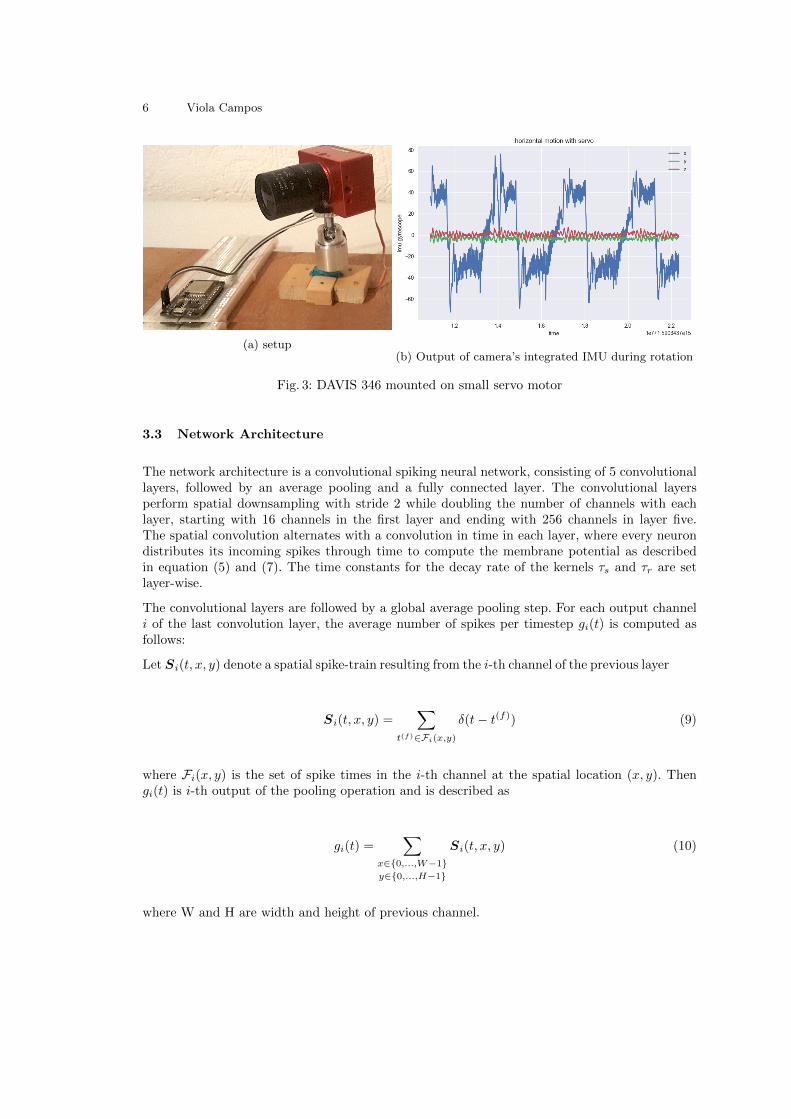
In order to record sequences at a constant rotational speed, the camera was mounted on aservo motor (RoVoR S0307) which was controlled by an Arduino board. It turned out thatthe recordings were unsuitable as training sequences, as the motor did not move the cameracontinuously, but in small steps. Figure 3 shows the setup and the IMU output of a samplesequence.

3.2 Preprocessing

SNNs operate on time-continuous data streams, so they must be discretized for simulation onGPUs. Choosing the discretization time steps means a trade-off between accuracy of the simula-tion (time steps as small as possible) and availability of memory and computational resources. Wechose time steps of 1 millisecond and restricted the simulation time to 100 milliseconds.

1 http://people.csail.mit.edu/jxiao/SUN360/

6 Viola Campos

(a) setup(b) Output of camera’s integrated IMU during rotation

Fig. 3: DAVIS 346 mounted on small servo motor

3.3 Network Architecture

The network architecture is a convolutional spiking neural network, consisting of 5 convolutionallayers, followed by an average pooling and a fully connected layer. The convolutional layersperform spatial downsampling with stride 2 while doubling the number of channels with eachlayer, starting with 16 channels in the first layer and ending with 256 channels in layer five.The spatial convolution alternates with a convolution in time in each layer, where every neurondistributes its incoming spikes through time to compute the membrane potential as describedin equation (5) and (7). The time constants for the decay rate of the kernels τs and τr are setlayer-wise.

The convolutional layers are followed by a global average pooling step. For each output channeli of the last convolution layer, the average number of spikes per timestep gi(t) is computed asfollows:

Let Si(t, x, y) denote a spatial spike-train resulting from the i-th channel of the previous layer

Si(t, x, y) =∑

t(f)∈Fi(x,y)

δ(t− t(f)) (9)

where Fi(x, y) is the set of spike times in the i-th channel at the spatial location (x, y). Thengi(t) is i-th output of the pooling operation and is described as

gi(t) =∑

x∈{0,...,W−1}y∈{0,...,H−1}

Si(t, x, y) (10)

where W and H are width and height of previous channel.

Spiking Networks for Event-Based Angular Velocity Regression 7

The last fully-connected layer connects these averaged spike-trains to three, non-spiking outputneurons for regressing the angular velocity prediction in time.

As we use the SNN for a regression task, we need to convert the output spike-train to numericvalues. This is done by convolving the spikes with the spike response kernel ε(·), similar to thecomputation of the post synaptic potential. To ensure a smooth function, it is reasonable tochoose a high value for τs in this layer. So the prediction of the angular velocity ω is

ω(t) = W (nl)(ε ∗ s(nl))(t) (11)

3.4 Loss function

The loss function L is taken from [GSMS20] and is defined as the time-integral over the eu-clidean distance between the predicted angular velocity ω(t) and ground truth angular velocityω(t):

L =1

T1 − T0

∫ T1

T0

√e(t)ᵀe(t)dt (12)

where e(t) = ω(t) − ω(t). To give the system some settling time, the evaluation of the errorfunction is only activated after processing the first 50 ms of the event sequence.

3.5 Training Procedure

The training of the SNN is based on first-order optimization methods, similar to backpropaga-tion in ANNs. Therefore, we must compute gradients of the loss function with respect to theparameters of the network. This is done with the publicly available PyTorch implementation 2 ofSLAYER [SO18], a backpropagation mechanism for supervised learning in deep spiking neuralnetworks.

To perform backpropagation in an SNN, two problems need to be solved: the state of the system isdetermined by the sequence of previous spikes, so it is uncertain how much each spike contributesto the error. The second problem is the non-differentiability of the spike function, so that anapproximation for the derivative is needed.

Further details on how error is assigned to previous time-points and how the derivative of thespike function is approximated with SLAYER can be found in [SO18].

4 Processing spikes with accurate timestamps

Actually, an SNN is a time-continuous dynamic system. To simulate it on GPUs, it must bediscretized, whereby the choice of step size means a trade-off between accuracy of the simulationand consumption of computational resources. We propose a new input format together with amodified processing pipeline to achieve higher accuracy in a discretized simulation.

We discretize the system with a sampling time Ts such that t = nTs, n ∈ Z and let Ns denotethe total number of samples in the period t ∈ [0, T ].

2 https://bitbucket.org/bamsumit/slayer/src/master/

8 Viola Campos

4.1 Spike Representation

Gehrig et al. use a binary discretized spike representation in [GSMS20]. Incoming events areassigned to sampling times. These ’time bins’ are stacked to a 4-dimensional vector of sizeC×H ×W ×Ns where C denotes the number of channels and H ×W are the input dimensions.Its entries are 1 if an event of the given channel is found at the corresponding pixel positionduring a time slice or 0 if no event was found. When this representation is used to computethe spike response signal to equation (1), the discrete time steps are used as spike times duringconvolution with the spike response kernel ε.

ε(t) =t

τse1−

tτsH(t), t ∈ nTs, n ∈ [0, Ns] (13)

Since the exact timestamps of the events are known (in µs-resolution), we use the entries inthe input vector to store the relative spike time ∆t during the time slice for events and zerootherwise. These exact spike times are used as additional information to compute more accuratesamples of the spike response signal. The discretized version of the spike response for a spikewith relative spike time ∆t becomes:

ε(t,∆t) =t

τse1−

tτsH(t), t ∈ nTs −∆t, n ∈ [0, Ns] (14)

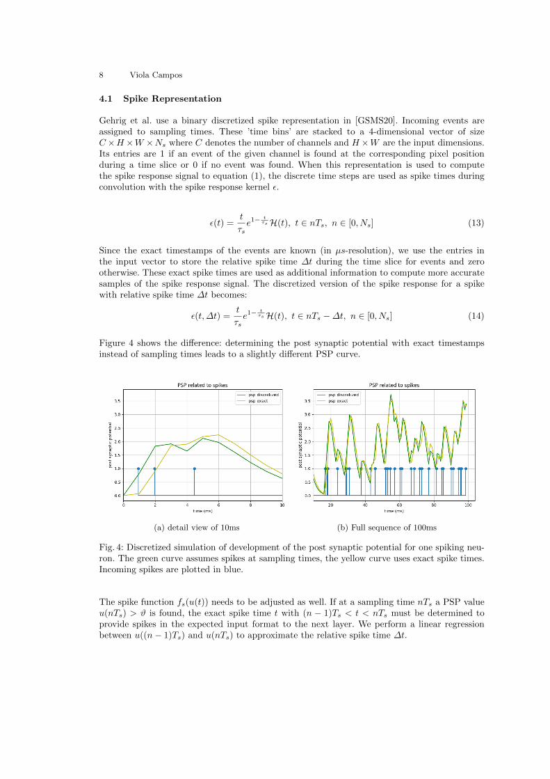
Figure 4 shows the difference: determining the post synaptic potential with exact timestampsinstead of sampling times leads to a slightly different PSP curve.

(a) detail view of 10ms (b) Full sequence of 100ms

Fig. 4: Discretized simulation of development of the post synaptic potential for one spiking neu-ron. The green curve assumes spikes at sampling times, the yellow curve uses exact spike times.Incoming spikes are plotted in blue.

The spike function fs(u(t)) needs to be adjusted as well. If at a sampling time nTs a PSP valueu(nTs) > ϑ is found, the exact spike time t with (n − 1)Ts < t < nTs must be determined toprovide spikes in the expected input format to the next layer. We perform a linear regressionbetween u((n− 1)Ts) and u(nTs) to approximate the relative spike time ∆t.

Spiking Networks for Event-Based Angular Velocity Regression 9

4.2 Average Pooling

The authors of [GSMS20] use an operation which they denote as global average spike pooling(GASP) to compute an averaged spike-train gi(t) (described in section 3.3).

gi(t) =1

W ·H∑

x∈{0,...,W−1}y∈{0,...,H−1}

Si(t, x, y) (15)

where Si(t, x, y) denotes the spatial spike-train resulting from the i-th channel of the previouslayer and W and H are width and height of the previous channel.

This pooling operation is pointless on spike-trains in our extended format as the average valueof an unspecified number of relative timesteps has no reasonable interpretation in the system.Instead, the pooling operation is modified to compute the average number of spikes per channeland timestep as intended.

5 Experiments

Based on the reference implementation3 from [GSMS20] we performed several experiments tofurther improve the accuracy of the regression.

Table 1 compares the root mean square error and the relative error of the predicted angularvelocities for simulated and real world data. While the absolute root mean squared error (RMSE)is slightly lower for the recorded event sequences than for the generated ones, the relative error ismuch higher. The reason for this is, that the mean angular velocity in the ’real world’ dataset islower than in the simulated dataset. Achieving low relative error at low absolute speed is difficultas the relative error converges towards infinite near zero angular velocity.

mean SNN

simulated data real world data simulated data real world data

RMSE (deg/s) 226.9 72.94 66.3 44.06

relative error 100% 100% 26% 54%

Table 1: Comparison of errors on different test sets. The naive mean prediction serves as abaseline.

Figure 6 illustrates the predicted angular velocities and ground truth for different samples ofevent sequences of 100ms. The plots show that the network needs some settling time beforeit predicts good values which corresponds with the training method: evaluation of the errorloss, backpropagation and weight updates are only performed after 50ms of the sequence duringtraining.

3 https://github.com/uzh-rpg/snn_angular_velocity

10 Viola Campos

To evaluate whether the starting time of loss evaluation influences the result, the SNN was trainedin different settings where evaluation of loss and penalizing errors started after 20ms, 30ms, 40msand 50ms. At the same time the error between predicted and ground truth angular velocity wasevaluated over different time periods starting from the whole sequence to the last 20ms only.Tables 2 and 3 give a comparison of errors after 40 epochs of training for these scenarios onsimulated and recorded event data. When trained on simulated data, the start time for trainingdoes not seem to to have a significant effect on the resulting accuracy of the network. Best resultsare achieved when training starts at 40ms but the results do only differ by a few degrees. Using’real world’ data, the results vary more, which is probably related to the quality of the inputdata.

Regarding the influence of the point in time at which the error evaluation begins, it is noticeablethat after a short settling time, the network already provides comparatively good predictionseven before the training has started. Here, the recursive character of the network is evident: ineach spiking layer the same operation is performed for every time step in the sequence.

Evaluate error after:

0ms 30ms 50ms 80ms

start training: RMSE relative error RMSE relative error RMSE relative error RMSE relative error

30 ms ... ... 56.37 0.69 47.73 0.57 46.78 0.56

40 ms ... ... 45.11 0.56 61.67 0.73 43.42 0.53

50 ms 49.47 0.63 41.25 0.51 44.10 0.54 43.31 0.54

Table 2: Comparison of different training scenarios for ’real world’ event sequences of 100ms.Root mean square error in deg/s and median of relative error are reported after 40 epochs oftraining for different combinations of starting times for error evaluation and backpropagation.

Evaluate error after:

0ms 30ms 50ms 80ms

start training: RMSE relative error RMSE relative error RMSE relative error RMSE relative error

30 ms 99.68 0.35 69.24 0.25 69.07 0.25 68.96 0.25

40 ms 98.06 0.35 66.89 0.25 66.79 0.25 66.62 0.25

50 ms 100.03 0.36 70.96 0.26 70.67 0.26 70.51 0.26

Table 3: Evaluation from table 2 on simulated event sequences.

5.1 Hyperparameter selection

As stated in [TGK∗19], the choice of suitable hyperparameters in spiking neural networks iscrucial for their learning ability. In the SRM neurons used in this work, the threshold value ϑ

Spiking Networks for Event-Based Angular Velocity Regression 11

in the spike generation function (3) influences how spikes propagate through the network. Ahigh value for ϑ reduces the rate of outgoing spikes compared to incoming ones, while a low ϑincreases the spike rate. The spike generation process in a layer is further influenced by τs and τr,temporal constants which define the decay rate of the spike response and the refractory kernelfrom equations (7) and (8). To ensure spike propagation until the output layer, ϑ, τs and τr mustbe chosen appropriately in relation to expected input spike rates to prevent both, vanishing andexploding signals.

Starting from the parameter set used in [GSMS20], we performed a grid search to optimize thehyper-parameters of the SNN for both simulated and recorded event data. Since Gehrig et al.increase the temporal parameters τs and τr with network depth and explain this choice as impor-tant to compensate for high event rates at the input layer and lower dynamics in deeper layers,the search focused on combinations of parameters which ensure a nearly constant number ofspikes per neuron in the individual layers. As this approach did not lead to significant improve-ments compared to the results from [GSMS20], the search was continued with more randomizedparameter combinations in a second step.

Against expectations, we achieved the best accuracy results with a set of constant parameters forall convolutional layers. In the fully connected layer which connects the pooling layer with thethree output neurons, a rather high value for τs worked best, as it lead to smoother predictions.After 40 epochs of training, our best model (Setup B in table 4) achieved a root mean squareerror of 49,2 deg/s which is a relative error of 17.1 % compared to 66.3 deg/s RMSE or a relativeerror of 26% from the original paper.

Figure 5 shows the development of the loss function for training and test data with exemplaryparameter settings and table 4 lists the hyperparameters used in each model in more detail. Allmodels are trained on the recorded event data set.

Fig. 5: Training and validation loss for different SNNs with same architecture and different hy-perparameters. For parameter settings see table 4.

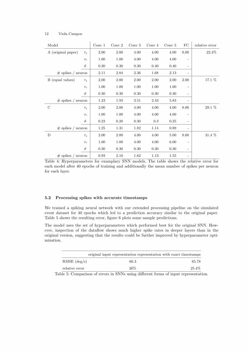
12 Viola Campos

Model Conv 1 Conv 2 Conv 3 Conv 4 Conv 5 FC relative error

A (original paper) τs 2.00 2.00 4.00 4.00 4.00 8.00 22.4%

τr 1.00 1.00 4.00 4.00 4.00 -

ϑ 0.30 0.30 0.30 0.40 0.40 -

# spikes / neuron 2.11 2.84 2.36 1.68 2.13 -

B (equal values) τs 2.00 2.00 2.00 2.00 2.00 2.00 17.1 %

τr 1.00 1.00 1.00 1.00 1.00 -

ϑ 0.30 0.30 0.30 0.30 0.30 -

# spikes / neuron 1.23 1.93 3.51 2.43 5.83 -

C τs 2.00 2.00 4.00 4.00 4.00 8.00 29.1 %

τr 1.00 1.00 4.00 4.00 4.00 -

ϑ 0.23 0.28 0.30 0.3 0.25 -

# spikes / neuron 1.25 1.31 1.82 1.14 0.89 -

D τs 2.00 2.00 4.00 4.00 5.00 8.00 31.4 %

τr 1.00 1.00 4.00 4.00 6.00 -

ϑ 0.30 0.30 0.30 0.30 0.30 -

# spikes / neuron 0.93 2.10 1.62 1.13 1.55 -

Table 4: Hyperparameters for examplary SNN models. The table shows the relative error foreach model after 40 epochs of training and additionally the mean number of spikes per neuronfor each layer.

5.2 Processing spikes with accurate timestamps

We trained a spiking neural network with our extended processing pipeline on the simulatedevent dataset for 40 epochs which led to a prediction accuracy similar to the original paper.Table 5 shows the resulting error, figure 6 plots some sample predictions.

The model uses the set of hyperparameters which performed best for the original SNN. How-ever, inspection of the dataflow shows much higher spike rates in deeper layers than in theoriginal version, suggesting that the results could be further improved by hyperparameter opti-mization.

original input representation representation with exact timestamps

RMSE (deg/s) 66.3 65.78

relative error 26% 25.4%

Table 5: Comparison of errors in SNNs using different forms of input representation.

Spiking Networks for Event-Based Angular Velocity Regression 13

6 Conclusions

In this work, we investigated an existing spiking neural network which uses backpropagation-based training to regress angular velocities on event-based data. It was shown that the networkis able to learn and predict angular velocities for recordings from a DVS instead of the simu-lated input data from the original work. Although the 3-DOF motion was more complex and thesensor introduced noise into the input data, the SNN was able to learn the angular velocities,however with less accuracy. We evaluated the influence of hyperparameters and training settingsand found better parameters for the proposed network. Further, a version of the SNN was de-veloped, which processes event data in a new input format which reduces errors in the inputrepresentation.

However, the accuracy of the predictions is still low compared to state-of-the-art ANNs in classicalcomputer vision while the backpropagation-based training approach is expensive in terms ofmemory consumption and processing time. Combining spiking neural nets with backpropagationas learning method does not feel like a natural choice. Backpropagation requires to unroll theSNN in time at discrete time steps which is expensive, introduces problems of recurrent networkslike vanishing and exploding gradients and does not correspond to the time-continuous nature ofthe system. Furthermore, in each time step the state of the whole network needs to be updated,which does not allow to address localized activity in the network and skip computations in idleareas.

We are still convinced, that the combination of spiking neural networks and even-based visionis promising. Nevertheless, in order to exploit the full potential of the technology, new learningapproaches are needed.

References

BDM∗17. Blum H., Dietmuller A., Milde M., Conradt J., Indiveri G., Sandamirskaya Y.:A neuromorphic controller for a robotic vehicle equipped with a dynamic vision sensor.Robotics Science and Systems, RSS 2017 (2017).

BTN15. Brosch T., Tschechne S., Neumann H.: On event-based optical flow detection. Frontiersin neuroscience 9 (2015), 137.

DFR∗17. Dikov G., Firouzi M., Rohrbein F., Conradt J., Richter C.: Spiking cooperativestereo-matching at 2 ms latency with neuromorphic hardware. In Conference on Biomimeticand Biohybrid Systems (2017), Springer, pp. 119–137.

GDO∗19. Gallego G., Delbruck T., Orchard G., Bartolozzi C., Taba B., Censi A.,Leutenegger S., Davison A. J., Conradt J., Daniilidis K., Scaramuzza D.: Event-based vision: A survey. ArXiv abs/1904.08405 (2019).

Ger95. Gerstner: Time structure of the activity in neural network models. Physical review. E,Statistical physics, plasmas, fluids, and related interdisciplinary topics 51 1 (1995), 738–758.

GK02. Gerstner W., Kistler W. M.: Spiking neuron models: Single neurons, populations, plas-ticity. Cambridge university press, 2002.

GSMS20. Gehrig M., Shrestha S. B., Mouritzen D., Scaramuzza D.: Event-based angularvelocity regression with spiking networks. arXiv preprint arXiv:2003.02790 (2020).

HH52. Hodgkin A. L., Huxley A. F.: A quantitative description of membrane current and itsapplication to conduction and excitation in nerve. The Journal of physiology 117, 4 (1952),500.

HWD∗20. He W., Wu Y., Deng L., Li G., Wang H., Tian Y., Ding W., Wang W., Xie Y.:Comparing snns and rnns on neuromorphic vision datasets: Similarities and differences.arXiv preprint arXiv:2005.02183 (2020).

14 Viola Campos

ICL18. Iyer L. R., Chua Y., Li H.: Is neuromorphic mnist neuromorphic? analyzing the discrimi-native power of neuromorphic datasets in the time domain. arXiv preprint arXiv:1807.01013(2018).

MBR∗18. Milde M. B., Bertrand O. J., Ramachandran H., Egelhaaf M., Chicca E.: Spikingelementary motion detector in neuromorphic systems. Neural computation 30, 9 (2018),2384–2417.

MGND∗19. Mozafari M., Ganjtabesh M., Nowzari-Dalini A., Thorpe S. J., Masquelier T.:Bio-inspired digit recognition using reward-modulated spike-timing-dependent plasticity indeep convolutional networks. Pattern Recognition 94 (2019), 87–95.

NMZ19. Neftci E. O., Mostafa H., Zenke F.: Surrogate gradient learning in spiking neuralnetworks: Bringing the power of gradient-based optimization to spiking neural networks.IEEE Signal Processing Magazine 36, 6 (2019), 51–63.

OBECT13. Orchard G., Benosman R., Etienne-Cummings R., Thakor N. V.: A spiking neuralnetwork architecture for visual motion estimation. In 2013 IEEE Biomedical Circuits andSystems Conference (BioCAS) (2013), IEEE, pp. 298–301.

OIBI17. Osswald M., Ieng S.-H., Benosman R., Indiveri G.: A spiking neural network modelof 3d perception for event-based neuromorphic stereo vision systems. Scientific reports 7(2017), 40703.

PVSDC19. Paredes-Valles F., Scheper K. Y. W., De Croon G. C. H. E.: Unsupervised learningof a hierarchical spiking neural network for optical flow estimation: From events to globalmotion perception. IEEE transactions on pattern analysis and machine intelligence (2019).

RGS18. Rebecq H., Gehrig D., Scaramuzza D.: Esim: an open event camera simulator. InConference on Robot Learning (2018), pp. 969–982.

SFJ∗20. Samadzadeh A., Far F. S. T., Javadi A., Nickabadi A., Chehreghani M. H.: Con-volutional spiking neural networks for spatio-temporal feature extraction. arXiv preprintarXiv:2003.12346 (2020).

SO18. Shrestha S. B., Orchard G.: Slayer: Spike layer error reassignment in time. In Advancesin Neural Information Processing Systems (2018), pp. 1412–1421.

SS17. Shrestha S. B., Song Q.: Robust learning in spikeprop. Neural Networks 86 (2017),54–68.

TGK∗19. Tavanaei A., Ghodrati M., Kheradpisheh S. R., Masquelier T., Maida A.: Deeplearning in spiking neural networks. Neural networks : the official journal of the InternationalNeural Network Society 111 (2019), 47–63.

Vre03. Vreeken J.: Spiking neural networks, an introduction.ZG18. Zenke F., Ganguli S.: Superspike: Supervised learning in multilayer spiking neural net-

works. Neural computation 30, 6 (2018), 1514–1541.

Spiking Networks for Event-Based Angular Velocity Regression 15

(a) DAVIS recording 1 (b) DAVIS recording 2

(c) Synthtic data 1 (d) Synthetic data 2

(e) Synthetic data, using exact timestamps 1 (f) Synthetic data, using exact timestamps 2

Fig. 6: Continuous-time angular velocity predicted by the SNN and corresponding ground truth.Upper row: ’real world’ data, center: synthetic event data, lower row: synthetic data processedwith a model, using spike representation from section 4 .