Behavioral/Systems/Cognitive

Spike-Timing Codes Enhance the Representation ofMultiple Simultaneous Sound-Localization Cues in theInferior Colliculus

Steven M. Chase and Eric D. YoungCenter for Hearing Sciences and Department of Biomedical Engineering, Johns Hopkins University, Baltimore, Maryland 21205

To preserve multiple streams of independent information that converge onto a neuron, the information must be re-represented moreefficiently in the neural response. Here we analyze the increase in the representational capacity of spike timing over rate codes usingsound localization cues as an example.

The inferior colliculus receives convergent input from multiple auditory brainstem nuclei, including sound localization informationsuch as interaural level differences (ILDs), interaural timing differences (ITDs), and spectral cues. Virtual space techniques were used tocreate stimulus sets varying in two sound-localization parameters each. Information about the cues was quantified using a spike distancemetric that allows one to separate contributions to the information arising from spike rate and spike timing.

Spike timing enhances the representation of spectral and ILD cues at timescales averaging 12 ms. ITD information, however, is carriedby a rate code. Comparing responses to frozen and random noise shows that the temporal information is mainly attributable to phaselocking to temporal stimulus features, with an additional first-spike latency component. With rate-based codes, there is significantconfounding of information about two cues presented simultaneously, meaning that the cues cannot be decoded independently. Spike-timing-based codes reduce this confounded information. Furthermore, the relative representation of the cues often changes as a functionof the time resolution of the code, implying that information about multiple cues can be multiplexed onto individual spike trains.

Key words: information theory; inferior colliculus; sound localization; spectral notch; ILD; ITD; spike distance metrics

IntroductionOften, single neurons in sensory systems respond to multiplestimulus features. Depending on how these features are coded inthe neural response, the brain may or may not have access to eachindividual feature. This leads to a natural question: how can mul-tiple stimulus features be multiplexed onto the responses of sin-gle neurons?

This question is of particular relevance in the auditory system.The central nucleus of the inferior colliculus (ICC) receives as-cending input from nearly every major brainstem nucleus (Rothet al., 1978; Adams, 1979; Brunso-Bechtold et al., 1981; Oliver etal., 1997) and is one of the first sites of convergence for the threemajor sound-localization cues: interaural level differences(ILDs), interaural timing differences (ITDs), and monaural spec-tral cues (SNs for spectral notches). Previous work has shownthat single ICC neurons display a range of sensitivity to localiza-tion cues, and most of the neural responses are modulated bymore than one cue (Benevento and Coleman, 1970; Caird andKlinke, 1987; Delgutte et al., 1995, 1999; Chase and Young, 2005).

This work, however, has all been based on the assumption of arate code. Although it is known that spike timing can also carryinformation in the auditory system (Rieke et al., 1992; Middle-brooks et al., 1994; Bandyopadhyay and Young, 2004; Nelken etal., 2005), it is not known how spike timing contributes to therepresentation of sound-localization cues in the ICC.

In this study, the coding of multiple localization cues in thespike trains of single ICC neurons is investigated using informa-tion theoretic techniques. Virtual-space stimulus sets were con-structed that vary independently in two sound-localization pa-rameters. Using a spike distance metric (SDM) developed byVictor and Purpura (1997), estimates of the mutual information(MI) between particular localization cues and the spike trains arecomputed at several different time resolutions. This approachallows one to separate out the contributions to information aris-ing from spike timing and spike rate.

The results show that spike-timing codes enhance the repre-sentation of all of the localization cues to some degree, with theexception of ITD, which is represented mainly by a rate code.Furthermore, the gain in timing information is almost entirelyattributable to phase locking to temporal stimulus features, suchas the envelope. The analysis allows the time resolution of thetemporal representation to be determined, suggesting that a tem-poral decoder would have to be sensitive to spike-timing coinci-dences of �12 ms to extract maximum information. Temporalcoding increases the degrees of freedom of the spike code in such

Received Nov. 22, 2005; revised Feb. 17, 2006; accepted Feb. 18, 2006.This work was supported by National Institutes of Health Grants DC00115, DC05211, and DC05742. We thank J.

Victor and D. Reich for making the code for SDM calculations freely available on-line.Correspondence should be addressed to Dr. Eric D. Young, 505 Traylor Research Building, 720 Rutland Avenue,

Baltimore, MD 21205. E-mail: eyoung@bme.jhu.edu.DOI:10.1523/JNEUROSCI.4986-05.2006

Copyright © 2006 Society for Neuroscience 0270-6474/06/263889-10$15.00/0

The Journal of Neuroscience, April 12, 2006 • 26(15):3889 –3898 • 3889

a way that multiple stimulus features can be independently rep-resented, which is not possible with only a rate code (Chase andYoung, 2005).

Materials and MethodsThis work is a new analysis of previously published data (Chase andYoung, 2005); the surgical procedure, recording protocol, and stimulusdesign were described in that paper and will be presented only brieflyhere.

Surgical procedure. Acute recording experiments were performed onadult cats with clean external ears, obtained from Liberty Labs (Waverly,NY). Animals were anesthetized for surgery with xylazine (1 mg/kg, i.m.)and ketamine (40 mg/kg, i.m.). The cat was decerebrated by transectingthe brain between the superior colliculus and the thalamus. After decer-ebration, anesthesia was discontinued. Throughout the experiment, thecat’s temperature was maintained between 37.5 and 38.5°C with afeedback-controlled heating pad.

The superior approach to the IC was achieved by aspirating occipitalcortex and, when necessary, removing part of the bony tentorium. Theear canals were exposed and fitted with ear tubes for sound delivery, andthe bullae on both sides were vented with 30 cm of polyethylene (PE 90)tubing. At the end of the experiment, the cat was killed with an overdoseof barbiturate anesthetic. All procedures were performed in accordancewith the guidelines of the Institutional Animal Care and Use Committeeof the Johns Hopkins University.

Recording procedure. All recordings were made in a sound-attenuatingchamber. Sounds were presented on speakers placed on hollow ear barsinserted into the ear canals. In situ speaker calibrations show responsesthat are uniform (�4.6 dB sound pressure level) between 40 Hz and 35kHz. Platinum/iridium microelectrodes were used for single-neuron re-cording; neurons were isolated with a Schmitt trigger or a template-matching program (Alpha-Omega Engineering, Nazareth, Israel). Alldata are based on clear single-neuron recordings.

Electrodes were advanced dorsoventrally through the IC to sampleneurons with various best frequencies (BFs). The BFs of isolated singleneurons were determined manually, and stimuli were presented to char-acterize the neurons according to the physiological categories defined byRamachandran et al. (1999). Briefly, neurons that were excited by mon-aural tones presented to either ear and that had little inhibition in theresponse map were classified as type V. Neurons whose responses tocontralateral BF tones were nonmonotonic, turning to inhibition at highsound levels, were classified as type O. Neurons that were excited at allcontralateral BF tone levels and displayed clear sideband inhibition wereclassified as type I. The majority of type I neurons were inhibited byipsilaterally presented tones.

Stimulus design. Three sets of virtual-space stimuli were created, basedon a 330 ms token of broadband noise (sampled at 100 kHz, interstimu-lus interval of 1 s). Each set was manipulated to vary independently intwo parameters, and each parameter was adjusted in five steps, for a totalof 25 stimuli per set. To build up statistics sufficient for informationtheoretic analyses, each stimulus set was repeated multiple times (20 –200, depending on how long the neuron was held) with the stimuli pre-sented in interleaved order.

In the first stimulus set, ITD and ILD were manipulated. The frozen-noise token was filtered through a spatially averaged head-related trans-fer function (HRTF) (obtained from the cat data of Rice et al., 1992),which imparts to the stimulus the spectral characteristics of the head andear canal, independent of spatial location. The stimulus was then splitinto two streams (one for each ear) that were delayed relative to oneanother to impart an ITD and attenuated relative to one another toimpart an ILD. ITDs and ILDs were chosen to correspond approximatelyto spatial locations in the horizontal plane of �60, �30, 0, 30, and 60°azimuth, in which negative values refer to locations in the ipsilateralhemifield (Kuhn, 1977; Roth et al., 1980; Rice et al., 1992) (cue values areprovided in Fig. 2).

In the second stimulus set, average binaural intensity (ABI) (com-puted as the mean sound pressure level across the two ears) and ILD were

manipulated. This set was designed to disambiguate monaural level re-sponses from true binaural sensitivity. In this case, the frozen noise wasagain filtered through the spatially averaged HRTF. The result was atten-uated to set an overall ABI (ranging from �8 to 8 dB in five equal steps)and then split into two streams that were attenuated relative to oneanother to impart an ILD that preserved that ABI.

In the third stimulus set, ILD and SN were varied. The SN cue wasimparted by filtering the frozen-noise token through one of five midlineHRTFs containing a prominent spectral notch, representing elevationsranging from 0 to 30° in 7.5° steps [Chase and Young (2005), their Fig. 2].The stimulus was then split into two streams, and an ILD cue was im-parted as in the ITD/ILD stimulus set. Interaural spectral differenceswere not considered in this work, because the same stimulus spectrumwas sent to each ear. Before presentation, the stimuli in this set wereresampled (resample command in Matlab; MathWorks, Natick, MA)such that the five SNs spanned the BF of the neuron under study with thenotch frequency of the third stimulus at BF. Note that this resamplingsometimes draws the SNs outside of the physiological range (6 –20 kHz)(Musicant et al., 1990; Rice et al., 1992). The resampling also changes thestimulus length. Stimuli longer than 400 ms were truncated at 400 ms,whereas stimuli shorter than 200 ms were repeated to be at least 200 mslong.

The stimuli described above were all created from a single sample ofnoise, a frozen noise. In this case, the analysis is sensitive to phase lockingto temporal stimulus features, which may be useful information for theauditory system but may or may not be a useful cue for sound localiza-tion. In a number of neurons, the SN/ILD stimulus set was modified touse a different noise on each stimulus presentation. In these cases, eachrepetition of the 25 SN/ILD stimuli was modified by adding a randomvector, sampled from the uniform distribution over [(0,2�), to the stim-ulus phases in the Fourier domain. This has the effect of randomizing thetemporal structure between sets of stimuli while holding the spectralmagnitudes constant. For the analysis done here, these stimuli eliminatedinformation in the stimulus envelope but preserved information in thespectral magnitudes. To minimize the effects of nonstationarity in theneural response, random-waveform sets were presented interleaved withthe frozen set.

Spike distance metric. The SDM developed by Victor and Purpura(1997) was used to assess the role of spike timing in conveying informa-tion. Essentially, the distance between two spike trains is defined as thesum of the costs of the elementary steps it takes to transform one spiketrain into the other. The allowed steps are spike deletion (cost of 1), spikeaddition (cost of 1), and spike shift (cost of q��t� ), where �t is the timedifference between a spike in one train and the nearest spike in the othertrain, and q is a variable cost parameter (units of s �1). For a given q, thereexists a minimum cost solution for the distance between any two spiketrains. A schematic of the distance calculation is presented in Figure 1 A.

The cost parameter q represents the precision with which spikes aretimed. If q��t� � 2, it is cheaper to add and delete a spike than it is to shiftit. Thus, 1/q is proportional to the time interval between spikes at whichthey are considered to be different, which can be interpreted as the inte-gration time of a neuron reading the spike train. If q � 0, the onlydistance assigned between spike trains is the difference in their absolutenumber of spikes, which represents a rate code. At the other extreme, asq approaches infinity, the reading neuron performs a coincidence detec-tor function in which spikes are not considered associated unless theyoccur at exactly the same time.

With the notion of spike-train distance defined, for any given spiketrain in response to stimulus i, it is possible to calculate the averagedistance to every other spike train measured from that neuron elicited bystimulus i, �d(i,i)�. This average distance can then be compared with theaverage distance between the spike train and every spike train elicited bystimulus j, �d(i,j)�. Figure 1 B illustrates this idea, in which the dots rep-resent spike trains and colors represent the stimuli being presented whenthe spike trains were measured. To a reading neuron, dots that clusterclosest together should produce the most similar responses. To computethe information between stimuli and spike-train distances, the spiketrains are assigned to the groups to which they are closest, regardless of

3890 • J. Neurosci., April 12, 2006 • 26(15):3889 –3898 Chase and Young • Spike-Timing Codes Enhance Localization Cues in IC

the actual stimulus. That is, the spike train i is estimated to have comefrom stimulus j when j satisfies

�di, j� � �di, k� � k � j. (1)

After repeating this process for every spike train, a confusion matrix N iscreated where N(i,j) represents the number of times a spike train from

stimulus i is classified as being closest to spike trains from stimulus j (Fig.1C). The confusion matrix, when normalized by the total number ofstimulus presentations, defines the joint stimulus/response probabilityon which MI (defined below) is calculated. As a stimulus estimationtechnique, the SDM allows the computation of a lower bound on the MIbetween stimuli and responses in a way analogous to other decodingtechniques (Kjaer et al., 1994; Rolls et al., 1997; Furukawa and Middle-brooks, 2002).

Because the distance metric is a function of q, the MI calculated withthis method is also a function of q. In addition to the q � 0 case, q was setto range from 10 to 15,850 s �1 (100 – 0.063 ms), sampled logarithmicallyat 5 costs per decade. These costs were found empirically to cover therelevant range of timing resolutions of the ICC neurons studied.

Spike trains beginning at stimulus onset and extending 20 ms paststimulus offset were used in this analysis. However, when comparing MIresults across neurons with different BFs, the analysis window was trun-cated at 200 ms to eliminate differences in stimulus length.

Mutual information. Responses were analyzed by computing the MIbetween stimulus and response. The response was defined either as thedischarge rate or as the result of the SDM calculation. The stimulus couldeither be the full 25 stimulus set containing variation of two stimulusparameters or a reduced set in which the variation of one stimulus pa-rameter was ignored so that a five stimulus set was defined by combiningthe stimuli across the other parameter.

The MI between the response of a neuron, R, and the stimulus, S, isdefined as follows (Cover and Thomas, 1991):

MIS; R � �s�S

�r�R

ps, rlog2� ps, r

pspr�. (2)

When the response is discharge rate, the MI is computed directly fromempirical distributions of spike counts; that is, p(s,r) is the probability ofgetting a certain spike count r for a stimulus s. This method, including thedebiasing methods, has been fully explained previously (Chase andYoung, 2005).

For the SDM method, MI was calculated from the confusion matrixdescribed above, in which s is the actual stimulus presented and r is theestimated stimulus from the cluster analysis. The probabilities were cal-culated from the counts in the confusion matrix, such that p(s,r) is theratio of the counts in a particular bin to the total count summed over thewhole matrix, and p(s) and p(r) are the ratios of the marginal counts tothe total count. The MI for the full stimulus set (25 stimuli) was com-puted from the full confusion matrix. The MIs for the two independentlyvarying cues were computed by combining the rows in the confusionmatrix having the same value of the parameter of interest.

For notational convenience, the information between the responseand the full stimulus set, MI(S;R), will be referred to as MIFULL, and theinformation between the response and an individual localization cue (Xor Y ) will be referred to as MIX or MIY. Mutual information calculatedfrom discharge rate is called rMI. The full information can be brokendown into the contributions from each localization cue as follows:

MIFULL � MIX � MIY � MIX; Y�R. (3)

A derivation of this equation is provided by Chase and Young (2005).Essentially, this equation emphasizes that the MI between the responseand the full stimulus set is always greater than or equal to the sum of theMIs about each of the individual cues, because the last term cannot benegative. MI(X;Y�R) is also known as the confounded information (Reichet al., 2001) and is related to the (lack of) independence in the neuralresponse. For example, when the spike count in response to parameter Xdepends on the value of parameter Y, the confounded information in thespike-rate code will be non-zero. More importantly, non-zero con-founded information means that the cues cannot be decodedindependently.

For this study, the maximum value of MIFULL is determined by thenumber of stimuli in the set. Because each of the stimulus sets in thisstudy consists of 25 stimuli presented with equal probability, MIFULL �

Figure 1. MI calculation using the spike distance metric. A, Spike distance calculation exam-ples. Left, To turn the top spike train into the bottom spike train, three spikes must be deleted.Right, To turn the top spike train into the bottom spike train, one spike must be deleted and twospikes shifted. This is the minimum-cost solution for all cost parameters q such that q�i � 2 @

i. When this condition is not met, the spike is deleted from its position in the top train and addedto the corresponding spot in the bottom train, adding a distance of 2. B, Stimulus clustering withthe SDM method. Each dot represents a spike train whose color denotes the stimulus playedwhen the train was recorded. For each train, the average distance �d(i,j)� to each group of spiketrains is calculated. The spike train is estimated to have come from the stimulus group to whichthe average distance is smallest. C, A confusion matrix counts the number of spike trains as-signed to each stimulus class. When normalized by the total number of spike trains, this is thejoint stimulus response matrix used to calculate the MI.

Chase and Young • Spike-Timing Codes Enhance Localization Cues in IC J. Neurosci., April 12, 2006 • 26(15):3889 –3898 • 3891

log2(25) � 4.6 bits. Similarly, MIX is bound from above by log2(5) � 2.3bits.

Estimates of MI based on finite datasets are subject to bias (Treves andPanzeri, 1995; Panzeri and Treves 1996; Paninski, 2003). For both therate and SDM methods, MI estimates were bias corrected with a boot-strap procedure (Efron and Tibshirani, 1998). In the rate case, 500 boot-strap datasets for each stimulus were derived by randomly drawing (withreplacement) M spike counts from the recorded set of spike counts forthat stimulus, where M is the number of stimulus repetitions. For theSDM case, 500 bootstrap confusion matrices were generated by ran-domly drawing (with replacement) from the counts of the confusionmatrix. That is, each row of the bootstrapped confusion matrix was gen-erated by selecting counts from the corresponding row of the originalmatrix, keeping the total count in each row fixed. In simulations, thisprocedure was found to converge to the true MI value faster than otherdebiasing methods, such as randomly reassigning stimuli and responses(data not shown). Data from neurons for which fewer than 20 repetitionsof each stimulus were gathered were not included in this analysis. Be-cause of the high number of stimulus repetitions typically achieved (me-dian of 70 repetitions), the estimated bias for MIFULL was quite low (rate,median of 0.11 bits; SDM peak, median of 0.08 bits). All values of MIpresented in this paper are bias corrected.

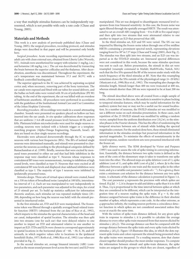
ResultsFigure 2 shows an example of a neuron studied with the ITD/ILDstimulus set presented at a high sound level. As often happens at

high levels, the rate response is saturated (Fig. 2A), so the rateinformation about the full stimulus set (rMIFULL) is only 0.3 bits.Although there is little consistent change in the spike countamong stimuli, a close-up view of the spike rasters (Fig. 2B)shows considerable variation in individual spike times with ILD.In particular, whereas the first burst is either on or off dependingon the ILD, the second, third, and fourth bursts are progressivelydelayed with increases in ILD. Figure 2C shows the results of theSDM analysis on these spike trains. For a spike-shift cost of 1000s�1, 1.6 bits of information is recovered about the stimulus iden-tity. This maximum is called MIpeak, and the cost at which itoccurs is called the peak cost. The cost � 0 case, which representsa rate code, is called MI0. Finally, the largest cost at which the MIdecays to half of its peak value is known as the cutoff cost, whichis �4000 s�1 for the neuron in Figure 2C. The MIs to the indi-vidual location cues are shown in Figure 2, D and E. As expectedfrom the raster plot, most of the information in MIFULL is aboutILD.

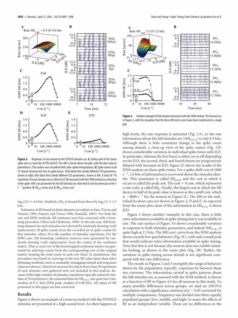
Figure 3 shows another example; in this case, there is littleextra information available in spike timing that is not available inrate. The rate surface of Figure 3A shows considerable variationin response to both stimulus parameters, and indeed rMIFULL isquite high at 2.3 bits. The MI(cost) curve from the SDM analysisshows a nearly low-pass behavior (Fig. 3C), with only a small peakthat would indicate extra information available in spike timing.Note that this is not because this neuron does not exhibit stimu-lus locking, as shown in the raster plot (Fig. 3B). Rather, thevariation in spike timing across stimuli is not significant com-pared with the rate differences.

The results in Figures 2 and 3 exemplify the range of behaviorshown by the population; typically, responses lie between thesetwo extremes. The information carried in spike patterns aboutthe full stimulus set, as assessed with the SDM method, is shownas a function of BF in Figure 4A for all neurons in this study. Toassess possible differences across groups, we used an ANOVAcalculation with a significance criterion of p � 0.05 corrected formultiple comparisons. Frequency was divided into three equallypopulated groups (low, middle, and high) to assess the effects ofBF as an independent variable. There are no differences in the

Figure 2. Responses of one neuron to the ITD/ILD stimulus set. A, Surface plot of the meanspike rate as a function of ITD and ILD. The rMI is shown above the plot, with the bias value inparentheses. (The surface was smoothed with cubic-spline interpolation.) B, Spike rasters to all25 stimuli showing the first six spike bursts. Thick black lines divide different ITD parameters,shown at right; thin black lines divide different ILD parameters, shown at left. A total of 110repetitions of each stimulus were collected. C, MI measured with the SDM method as a functionof the spike-shift cost parameter for the full stimulus set. Note that 0 cost has been put at the 1s �1 position. D, MIILD versus cost. E, MIITD versus cost.

Figure 3. Another example of information extraction with the SDM method. The format is asin Figure 2, with the exception that the three MI(cost) curves have been condensed to a singleplot.

3892 • J. Neurosci., April 12, 2006 • 26(15):3889 –3898 Chase and Young • Spike-Timing Codes Enhance Localization Cues in IC

MIpeak values across the three stimulus sets, so they are not dif-ferentiated in this plot. There are also no differences in MIpeak

across the neuron types or in differences in MIpeak values with BF.To view the amount of information available in temporal

spike patterns that is not available in spike rate, MIpeak from theSDM calculation is plotted as a function of the information cal-culated assuming a rate code in Figure 4B. The vertical offset ofthe points from the diagonal represents the extra informationavailable when spike timing is taken into account. Many neuronsshow a considerable information gain with the SDM method.

Recall that, for the 0 cost (q � 0) analysis, no penalty is as-signed to shifting spikes, only to adding or deleting them. Thiscase should, then, correspond to a rate code, and the informationcalculated from the SDM method at 0 cost should be the same asthe information calculated under the assumption of a rate code, ifno information is lost in the decoding step when the confusionmatrix is generated. When MI0 is plotted as a function of rMI foreach neuron, there is very good agreement between the two mea-surements (r � 0.99) (Fig. 4C).

In Figure 5, MIpeak values are compared with the correspond-

ing rMI measures for each of the individ-ual localization cues. For ITD information(Fig. 5A), the points all cluster along thediagonal, showing that very little extra in-formation is available when consideringspike timing. This strongly suggests that,at the level of the ICC, ITD information iscarried in a rate code. The coding of ILDcues is shown in Figure 5B, in which ILDcues from all three stimulus sets have beenlumped together because the populationsoverlap. The SDM method recovers a mildamount of information about ILD cuesover that available through a rate code.The same holds true for ABI cues (Fig.5C), which show less information, on av-erage, than the other cues. The largest ef-fect of spike timing is on the coding of SNcues (Fig. 5D). In general, the MI in SDMresponses to SN is much larger than theMI in rate responses to SN. For some neu-rons, as much as 2 bits of information isrecovered by considering spike timing.

The spike-timing gain for SN informa-tion is plotted as a function of BF in Figure5E. This gain is defined as the differencebetween MIpeak and MI0 and representsinformation only available through spiketiming. The spike-timing gain is nega-tively correlated with BF (r � �0.48; df �56; p � 0.0001); it is mainly the low-BFneurons that carry the extra informationabout SN in the timing of spikes, althoughthere are some midfrequency neuronswith spike-timing gains of as much as 1bit. The largest spike-timing gains are seenin type V neurons, which are found only atlow BFs (Ramachandran et al., 1999) andare the predominant low-BF responsetype in our sample. This point is discussedin more detail in Discussion.

Timescale of informationThe cost at which MI is maximum is a measure of the temporalprecision of the spike patterns that provide information capturedby the SDM analysis. As discussed in Materials and Methods, 1/qis a measure of the effective integration time of a neuron readingthe temporal information in spike patterns, in the sense that 2/q isthe maximum time delay between spikes in two trains at whichthey can still be shifted into alignment.

Figure 6 shows data on the costs at which the maximum MI isobtained with the SDM analysis, for each of the localization cuesstudied. The median peak cost value obtained by pooling costvalues from all localization cues and ignoring 0 values is �80 s�1.Thus, when there is localization information in spike timing, it isintegrated on a timescale of �12 ms.

A peak cost of 0 was declared if the MIpeak value remainedwithin 10% of MI0 for that neuron (for example, the ILD curve inFig. 3C), indicating that most of the information was carried byrate. Peak costs of 0 occurred in 50% of the ITD cases (Fig. 6A)and 41% of the ILD cases (Fig. 6B). This is in comparison withonly 12% of cases for the ABI cue (Fig. 6C) and 9% of cases for theSN cue (Fig. 6D).

Figure 4. SDM information carried about the full stimulus set. V, I, and O symbols correspond to the physiological neuron type.A, MIpeak plotted as a function of BF for all neurons and stimuli. B, MIpeak as a function of the information calculated directly fromthe spike rates. C, MI from the SDM method at 0 cost plotted as a function of the MI calculated directly from discharge rate.

Figure 5. Comparison between the peak information calculated with the SDM method and rMI for individual localization cues.A, ITD. B, ILD. C, ABI. D, SN. E, Spike-timing gain (MIpeak � MI0) as a function of BF for the SN cue.

Chase and Young • Spike-Timing Codes Enhance Localization Cues in IC J. Neurosci., April 12, 2006 • 26(15):3889 –3898 • 3893

The other major difference between the information time-scales for different localization cues is that there is a significantcorrelation between BF and peak cost for the SN cue (r � �0.46;df � 48; p � 0.0004, ignoring 0 cost values) that is not seen withthe other cues. SNs are represented at finer timescales in low-BFneurons than they are in high-BF neurons.

Frozen versus random noiseIn this section, we show that the information that is recovered bythe SDM analysis is almost entirely derived from locking to tem-poral features of the stimulus. To demonstrate this point, re-sponses to frozen noise, for which the temporal waveform is thesame in all stimulus repetitions, were compared with responses tophase-randomized noise, for which the temporal waveform dif-fers in each repetition. Information that depends on the tempo-rally locked stimulus features will not be present with the randomnoise. All data presented to this point were obtained with frozennoise.

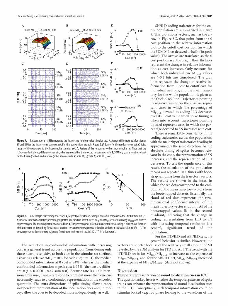
Figure 7 shows the responses of a 1.8 kHz type O neuron inresponse to the random/frozen stimulus set described in Materi-als and Methods. There is very little difference in the average rateresponses, as shown in Figure 7, A and B, and the rMIFULL of thesestimulus sets are nearly identical at �0.65 bits. The temporalresponses to the two stimulus sets are completely different, how-ever, as shown by the raster plots in Figure 7, C and D. From theraster to the frozen noise, it is clear that this neuron responded tospecific temporal events in the stimuli, events that occur at fixedtimes in the frozen noise but not in the random noise. As anexample, there is a spike that occurs frequently at a latency of �56ms in the responses to two of the frozen SN stimuli (1.8 and 1.7kHz) but not in the others. The only apparent temporal featurethat remains in the random noise is the latency of the first burst ofspikes, which changes systematically with ILD in both stimulussets.

The SDM information carried by this neuron is shown inFigure 7E–G for both stimulus sets. As is characteristic of low-frequency neurons, there is a large peak in the MI(cost) curves forthe frozen-noise set, indicating the presence of a substantialamount of information in spike timing over that in rate. Thesepeaks are missing from the random-waveform responses. Thus,the extra information available in spike timing was attributable tothe differences in the temporal waveforms within the frozen-noise SN/ILD stimulus set as opposed to an intrinsic variation inspike patterns stemming purely from spectral or level differences.

ILD-related latency differences were observed in both the re-sponses to frozen and random waveforms (Fig. 7C,D). However,the SDM method reveals timing information in only the frozen-waveform case. This indicates that the SDM method, as com-puted here, is relatively insensitive to first-spike-latency varia-tion. Although differences in spike latency must increase thedistance between spike trains, this distance is apparently over-whelmed by other noisy sources of spike-train differences. Whenthe SDM MI is computed using spike trains with all but the firstspike removed (a first-spike latency code), 1.3 and 0.9 bits ofinformation are recovered about the full stimulus set for thefrozen- and random-waveform sets, respectively.

The results of the example neuron in Figure 7 are consistentacross the population of neurons for which the random-waveform stimulus data were gathered. For the 13 neurons stud-ied with the random-noise stimuli, the mean and SD of the spiketiming gains for frozen noise were 0.54 � 0.61 bits (range of0 –1.7 bits), whereas the corresponding spike-timing gain valuesfor random noise were significantly less at 0.1 � 0.06 bits (rangeof 0 – 0.25 bits; different from frozen noise at p � 0.01, signedrank test). ILD random-noise spike-timing gains were not signif-icantly different from SN gains.

Relative informationThe percentage of MIFULL that is devoted to the coding of anindividual localization cue is called the relative information. It iscomputed as the ratio MIX/MIFULL and is the basis for analyzingthe interactions of individual localization cues. An example ofthis computation is given in Figure 8 for a type V neuron inresponse to the SN/ILD stimulus set (with frozen noise). Figure8A shows MIFULL, MIILD, and MISN as a function of cost. At �630s�1, this neuron shows a prominent peak of 3.5 bits in its MIFULL-

(cost) curve (one of the most sensitive neurons in the popula-tion), a gain of �2 bits over its 0 cost value. Although it is clearfrom Figure 8A that MIILD and MISN covary with MIFULL, Figure8B shows that the fraction of MIFULL devoted to ILD or SN cod-ing is not constant with cost. Instead, there is a monotonic in-crease in the MISN percentage as a function of cost, whereas MIILD

shows a low-pass behavior.This result is further summarized in Figure 8C. Here, the “tra-

jectory” of single-cue coding is plotted. Each dot plots the relativeinformation for SN versus ILD at a particular cost. Points liebelow the diagonal when MIFULL is not equal to the sum of theinformation in the individual cues or when the confounded in-formation of Equation 3 is non-zero. At a cost of 0 (rate case), theconfounded information is large; MISN and MIILD are not inde-pendently represented in the neural response. As the cost param-eter is increased, the confounded information decreases until itreaches 0 (near 50 s�1), signifying that SN and ILD are indepen-dently coded. Finally, at costs over 1000 s�1, the informationabout both ILD and SN (and MIFULL) decreases. The decrease isfaster for ILD, so the points in Figure 8C move toward the upperleft-hand corner of the plot.

Figure 6. Timescale of the temporal representation of localization cues. A, Cost at which theSDM MI reached its peak value plotted as a function of BF for the ITD cue. Note that the 0 costdata points have been placed at the 1 s �1 spot. B, ILD. C, ABI. D, SN. The black line representsthe best linear fit of log(cost) to log(BF), ignoring 0 cost values.

3894 • J. Neurosci., April 12, 2006 • 26(15):3889 –3898 Chase and Young • Spike-Timing Codes Enhance Localization Cues in IC

The reduction in confounded information with increasingcost is a general trend across the population. Considering onlythose neurons sensitive to both cues in the stimulus set (definedas having a relative rMIX 10% for each cue; n � 94), the medianconfounded information at 0 cost is 24%, whereas the medianconfounded information at peak cost is 15% (the two are differ-ent at p � 0.00001, rank sum test). Because rate is a unidimen-sional measure, using a rate code to represent more than one cuenecessarily leads to a confounded representation of the encodedquantities. The extra dimensions of spike timing allow a moreindependent representation of the localization cues and, in the-ory, allow the cues to be decoded more independently, as well.

SN/ILD coding trajectories for the en-tire population are summarized in Figure9. This plot shows vectors, such as the ar-row in Figure 8C, that point from the 0cost position in the relative informationplot to the cutoff cost position (in whichthe SDM MI has decayed to half of its peakvalue). The arrows are translated so the 0cost position is at the origin; thus, the linesrepresent the changes in relative informa-tion as cost increases. Only neurons forwhich both individual cue MIpeak valuesare �0.2 bits are considered. The graylines represent the change in relative in-formation from 0 cost to cutoff cost forindividual neurons, and the mean trajec-tory for the whole population is given asthe thick black line. Trajectories pointingto negative values on the abscissa repre-sent cases in which the percentage ofMIFULL devoted to coding ILD decreasesover its 0 cost value when spike timing istaken into account; trajectories pointingupward represent cases in which the per-centage devoted to SN increases with cost.

There is remarkable consistency in thecoding trajectories across the population,with the majority of trajectories heading inapproximately the same direction. As theabsolute timing of spikes becomes rele-vant in the code, the representation of SNincreases, and the representation of ILDdecreases. To test the significance of thisresult, the calculation of the populationmeans was repeated 1000 times with boot-strap sampling from the trajectory vectors.The results are shown in the inset, inwhich the red dots correspond to the end-points of the mean trajectory vectors fromthe bootstrapped datasets. Essentially, thecloud of red dots represents the two-dimensional confidence interval of themean trajectory vector endpoint. All of thebootstrapped values lie in the secondquadrant, indicating that the change incoding representation from ILD to SNwith increasing temporal resolution is ageneral, significant trend of thepopulation.

For the ITD/ILD and ABI/ILD sets, thegeneral behavior is similar. However, the

vectors are shorter because of the relatively small amount of MIrevealed by the SDM analysis for ITD and ABI. The trend with theITD/ILD set is for MIILD/MIFULL to increase at the expense ofMIITD/MIFULL, and, for the ABI/ILD set, MIABI/MIFULL increasedat the expense of MIILD/MIFULL (data not shown).

DiscussionTemporal representation of sound localization cues in ICCThe question asked here is whether the temporal patterns of spiketrains can enhance the representation of sound localization cuesin the ICC. Conceptually, such temporal information could bestimulus locked (e.g., by phase locking to the waveform of the

Figure 7. Responses of a 1.8 kHz neuron to the frozen- and random-noise stimulus sets. A, Average firing rate as a function ofSN and ILD for the frozen-noise stimulus set. Plotting conventions are as in Figure 2. B, Same, for the random-noise set. C, Spikerasters of the responses to the frozen-noise stimulus set. D, Rasters of the responses to the random-noise set. Note that theILD-dependent latency differences remain, whereas most other time-locked responses vanish. E, SDM MIFULL as a function of costfor the frozen (dotted) and random (solid) stimulus sets. F, SDM MIILD(cost). G, SDM MISN(cost).

Figure 8. An example cost/coding trajectory. A, MI(cost) curves for an example neuron in response to the SN/ILD stimulus set.B, Relative information [MI (as percentage)] plotted as a function of cost. Here, MISN and MIILD are normalized by MIFULL and plottedas percentages. Their sum is plotted as a dotted line. C, The percentage of information devoted to SN coding is plotted as a functionof that devoted to ILD coding for each cost studied; certain trajectory points are labeled with their cost values (units of s �1). Thearrow represents the summary trajectory from 0 cost to the cutoff cost (6310 s �1 for this neuron).

Chase and Young • Spike-Timing Codes Enhance Localization Cues in IC J. Neurosci., April 12, 2006 • 26(15):3889 –3898 • 3895

stimulus), or not stimulus locked. In the latter case, sound local-ization cues would be represented by changes in the temporalpatterns of spiking that are not directly related to the temporalwaveform of the stimulus, as in the work in visual cortex byOptican and Richmond (Optican and Richmond, 1987; Rich-mond and Optican, 1990). Of course, most auditory neurons,including those in the ICC, lock strongly to the stimulus en-velope (Joris, 2003; Louage et al., 2003). Thus, evaluation ofnonstimulus-locked temporal coding must control for these en-velope responses; here we used random noise, for which envelopelocking should not provide consistent information from onestimulus to the next.

We use an SDM analysis to look at temporal coding. An im-portant check on this analysis is the fact that the 0 cost MI is thesame as the discharge rate MI (rMI � MI0 in Fig. 4C). Because theSDM method is based on stimulus parameter estimation, it pro-vides a lower bound to the information available in the spiketrains. For the 0 cost case, the SDM method recovers all of theinformation available; however, this is not true at higher costs,because we know the method is insensitive to first-spike-latencyinformation (discussed below). Thus, the information incrementanalysis (Fig. 5) should be looked on as a lower bound to the extratemporal information that is available in spike trains.

The results show that encoding in spike timing potentiallyenhances the amount of information carried about localizationcues in ICC (Figs. 4, 5). Significant timing-dependent incrementswere seen for all of the cues except ITD, with the largest effects forSN. The lack of ITD-related temporal information suggests thatITD is represented by discharge rate alone in ICC. This is consis-tent with the work of Carney and Yin (1989), who investigatedthe effects of ITD manipulation in a population of low-frequencyICC neurons. Their raster plots of neurons responding to broad-band noise at various ITDs (compare with their Figs. 10, 11) show

that there is little change in the timing of spikes to changes in ITD;rather, there is a large ITD-dependent gain change.

The position of the peak in MI versus cost functions (Fig.2C–E) provides an estimate of the timescale at which spike timingprovides the most information. The data of Figure 6 show thatlocalization cues in the ICC are best decoded at a cost of �80s �1, suggesting that the resolution of localization-relatedspike-timing patterns in the ICC is �12 ms.

The nature of the temporal representationWhen random noise was used to eliminate stimulus-waveformcues, the only temporal information remaining in IC neuronswas that encoded in first-spike latency. Sound location has beenshown to modulate the first-spike latency in both IC and auditorycortex (Brugge et al., 1996; Furukawa and Middlebrooks, 2002;Sterbing et al., 2003; Mrsic-Flogel et al., 2005). Although latencydifferences contribute to the distances measured with the SDM,in practice, the variation in spike-train distances caused by la-tency are too small to have much effect on stimulus grouping,unless the analysis is confined to the first few spikes. Theanalysis of temporal information presented here does not ad-dress the role that first-spike latency may play in encodingsound-localization cues.

The frozen/random-noise analysis (Fig. 7) shows that thetemporal patterns are mainly locked to temporal features of thestimulus waveform, independent of static localization cue values.The largest stimulus-waveform effects are related to SN cues.Presumably, these represent phase locking to the temporal enve-lope of the stimulus induced by the sharp antiresonances in theSN stimuli. The strongest temporal information about SN occursat BFs below the physiological range of SN cues in cats (Musicantet al., 1990; Rice et al., 1992). This suggests that the temporalincrements for SN stimuli do not represent a specialization forrepresenting SN. Instead, the temporal information is induced byspectral irregularities or temporal envelopes in general, as forexample in speech (Bandyopadhyay and Young, 2004).

Can the temporal information identified here be used by theauditory system for sound localization? To do so, there wouldhave to be a template for the spike trains expected from a knownstimulus (i.e., the stimulus would have to be recognized by theauditory system on the basis of its other properties). Then itslocation could be determined in part through the envelope in-duced by SN cues as demonstrated here. However, this source ofinformation would be vulnerable to echoes and other environ-mental phase distortions, limiting its usefulness as an absolutelocalization cue.

A situation in which temporal cues might contribute is whencomparisons of two stimuli occurring in the same acoustic envi-ronment are possible (e.g., in determining when a given soundsource has changed location). In binaural-masking-level-difference experiments, random noises are more effective atmasking interaural correlation differences than frozen noises(Breebaart and Kohlrausch, 2001) because of the uncertainty inthe interaural correlation of the masker. This result suggests thatminimum audible angles for random-noise stimuli should behigher than for frozen stimuli, because of better encoding of SNcues in the latter case. Another situation in which temporal lock-ing would be useful would be in the comparison of spike timesacross different neurons. This type of population encoding is notconsidered in this analysis.

Perhaps more surprising than the temporally locked SN infor-mation is the temporally locked ILD information. ILD is a staticcue, yet its representation in the neural response benefits from

Figure 9. Cost coding summary trajectories for the population in response to the SN/ILDstimulus set. Individual coding trajectories are shown in gray, and the population mean isshown in black. The inset shows a close-up view of the population mean. Red dots representpopulation means resulting from bootstrap resampling of the individual trajectories; 1000bootstrap samples were used.

3896 • J. Neurosci., April 12, 2006 • 26(15):3889 –3898 Chase and Young • Spike-Timing Codes Enhance Localization Cues in IC

spike times locked to the stimulus. When the ILD is changed,events in the stimulus that were subthreshold could become su-perthreshold and cause the neuron to spike. These spikes wouldforce the neuron into its refractory period and may affect theposition of the next burst of spikes. Thus, changes in ILD couldcause a rearrangement in the peristimulus time histogram(PSTH). Of course, the same argument could be made forchanges in ITD, which do not result in rearrangements in thePSTH; the mechanisms behind ILD and ITD encoding need to befurther explored.

Differences among ICC neuron classesIn a previous publication (Chase and Young, 2005), the informa-tion about localization cues provided by ICC neurons of threedifferent response types was compared. That analysis, based onlyon discharge rate, found that, although there were some differ-ences among the neuron types, generally there was substantialoverlap in the information provided by the three classes of neu-rons. The largest differences were for the type V neurons, whichprovided information mainly about ITD and ABI. Type V neu-rons stand out in the present analysis by showing larger MI in-crements than the other neuron types when spike timing is con-sidered. Because type V neurons are found only at low BFs andbecause most of the neurons in the low-BF sample were type V, itis not clear whether the difference has to do with BF or with theparticular circuitry connected to the type V neurons. An argu-ment for the former is that the changes in temporal envelopeproduced by shifting the location of a spectral notch will be athigher envelope frequencies for high-BF neurons compared withlow-BF neurons. Given that neurons in the ICC have a cutofffrequency in their modulation transfer functions of �100 Hz(Langner and Schreiner, 1988; Krishna and Semple, 2000), it maybe that the temporally coded information produced by changes inSN frequency is outside the modulation response regions of neu-rons or high-BF neurons.

The representation of multiple cuesThese results show that spike-timing codes can reduce the con-founded information in the response, allowing individual cues tobe represented more independently (Figs. 8, 9). Furthermore, therepresentation of cues in the response changes as a function of thedecoding time resolution in a consistent manner, as illustratedfor SN/ILD stimuli by Figure 9. ITDs are coded on the longesttimescales, by spike rate. ILDs are coded at intermediate time-scales because increases in the SDM cost cause an increase in ILDinformation relative to ITD information but a decrease relative toSN information. SN information is available at the shortest time-scales, especially in low-frequency neurons. Together, these re-sults imply that spike timing could play an important role inmultiplexing information onto spike trains, given appropriatedecoding mechanisms.

ReferencesAdams JC (1979) Ascending projections to the inferior colliculus. J Comp

Neurol 183:519 –538.Bandyopadhyay S, Young ED (2004) Discrimination of voiced stop conso-

nants based on auditory nerve discharges. J Neurosci 24:531–541.Benevento LA, Coleman PD (1970) Responses of single cells in cat inferior

colliculus to binaural click stimuli: combinations of intensity levels, timedifferences, and intensity differences. Brain Res 17:387– 405.

Breebaart J, Kohlrausch A (2001) The influence of interaural stimulus un-certainty on binaural signal detection. J Acoust Soc Am 109:331–345.

Brugge JF, Reale RA, Hind JE (1996) The structure of spatial receptive fields

of neurons in primary auditory cortex of the cat. J Neurosci16:4420 – 4437.

Brunso-Bechtold JK, Thompson GC, Masterton RB (1981) HRP study ofthe organization of auditory afferents ascending to central nucleus ofinferior colliculus in cat. J Comp Neurol 197:705–722.

Caird D, Klinke R (1987) Processing of interaural time and intensity differ-ences in the cat inferior colliculus. Exp Brain Res 68:379 –392.

Carney LH, Yin TCT (1989) Responses of low-frequency cells in the inferiorcolliculus to interaural time differences of clicks: excitatory and inhibitorycomponents. J Neurophysiol 62:144 –161.

Chase SM, Young ED (2005) Limited segregation of different types of soundlocalization information among classes of units in the inferior colliculus.J Neurosci 25:7575–7585.

Cover TM, Thomas JA (1991) Elements of information theory. New York:Wiley.

Delgutte B, Joris PX, Litovski RY, Yin TCT (1995) Relative importance ofdifferent acoustic cues to the directional sensitivity of inferior-colliculusneurons. In: Advances in hearing research (Manley GA, Klump GM,Koppl C, Fastl H, Oeckinghaus H, eds), pp 288 –299. River Edge, NJ:World Scientific.

Delgutte B, Joris PX, Litovski RY, Yin TCT (1999) Receptive fields and bin-aural interactions for virtual-space stimuli in the cat inferior colliculus.J Neurophysiol 81:2833–2851.

Efron B, Tibshirani RJ (1998) Introduction to the bootstrap. Boca Raton,FL: CRC.

Furukawa S, Middlebrooks JC (2002) Cortical representation of auditoryspace: information-bearing features of spike patterns. J Neurophysiol87:1749 –1762.

Joris PX (2003) Interaural time sensitivity dominated by cochlea-inducedenvelope patterns. J Neurosci 23:6345– 6350.

Kjaer TW, Hertz JA, Richmond BJ (1994) Decoding cortical neuronal sig-nals: network models, information estimation and spatial tuning. J Com-put Neurosci 1:109 –139.

Krishna BS, Semple MN (2000) Auditory temporal processing: responses tosinusoidally amplitude-modulated tones in the inferior colliculus. J Neu-rophysiol 84:255–273.

Kuhn GF (1977) Model for the interaural time differences in the azimuthalplane. J Acoust Soc Am 62:157–167.

Langner G, Schreiner CE (1988) Periodicity coding in the inferior colliculusof the cat. I. Neuronal mechanisms. J Neurophysiol 60:1799 –1822.

Louage DHG, van der Heijden M, Joris PX (2003) Temporal properties ofresponses to broadband noise in the auditory nerve. J Neurophysiol91:2051–2065.

Middlebrooks JC, Clock AE, Xu L, Green DM (1994) A panoramic code forsound location by cortical neurons. Science 264:842– 844.

Mrsic-Flogel TD, King AJ, Schnupp JWH (2005) Encoding of virtual acous-tic space stimuli by neurons in ferret primary auditory cortex. J Neuro-physiol 93:3489 –3503.

Musicant AD, Chan JCK, Hind JE (1990) Direction-dependent spectralproperties of cat external ear: new data and cross-species comparisons. JAcoust Soc Am 30:237–246.

Nelken I, Chechik G, Mrsic-Flogel TD, King AJ, Schnupp JWH (2005) En-coding stimulus information by spike numbers and mean response timein primary auditory cortex. J Comp Neurosci 19:199 –221.

Oliver DL, Beckius GE, Bishop DC, Kuwada S (1997) Simultaneous antero-grade labeling of axonal layers from lateral superior olive and dorsalcochlear nucleus in the inferior colliculus of cat. J Comp Neurol382:215–229.

Optican LM, Richmond BJ (1987) Temporal encoding of two-dimensionalpatterns by single units in primate primary visual cortex. I. Informationtheoretic analysis. J Neurophysiol 57:162–178.

Paninski L (2003) Estimation of entropy and mutual information. NeuralComput 15:1191–1253.

Panzeri S, Treves A (1996) Analytical estimates of limited sampling bi-ases in different information measures. Netw Comput Neural Syst7:87–107.

Ramachandran R, Davis KA, May BJ (1999) Single-unit responses in theinferior colliculus of decerebrate cats. I. Classification based on frequencyresponse maps. J Neurophysiol 82:152–163.

Reich DS, Mechler F, Victor JD (2001) Formal and attribute-specific infor-mation in primary visual cortex. J Neurophysiol 85:305–318.

Richmond BJ, Optican LM (1990) Temporal encoding of two-dimensional

Chase and Young • Spike-Timing Codes Enhance Localization Cues in IC J. Neurosci., April 12, 2006 • 26(15):3889 –3898 • 3897

patterns by single units in primate primary visual cortex. II. Informationtransmission. J Neurophysiol 64:370 –380.

Rice JJ, May BJ, Spirou GA, Young ED (1992) Pinna-based spectral cues forsound localization in cat. Hear Res 58:132–152.

Rieke F, Yamada W, Moortgat K, Lewis ER, Bialek W (1992) Real timecoding of complex sounds in the auditory nerve. Adv Biosci83:315–322.

Rolls ET, Treves A, Tovee MJ (1997) The representational capacity of thedistributed encoding of information provided by populations of neuronsin primate temporal visual cortex. Exp Brain Res 114:149 –162.

Roth GL, Aitkin LM, Andersen RA, Merzenich MM (1978) Some features of

the spatial organization of the central nucleus of the inferior colliculus ofthe cat. J Comp Neurol 182:661– 680.

Roth GL, Kochar RK, Hind JE (1980) Interaural time differences: implica-tions regarding the neurophysiology of sound localization. J Acoust SocAm 68:1643–1651.

Sterbing SJ, Hartung K, Hoffmann K (2003) Spatial tuning to virtual soundsin the inferior colliculus of the guinea pig. J Neurophysiol 90:2648 –2659.

Treves A, Panzeri S (1995) The upward bias in measures of informationderived from limited data samples. Neural Comput 7:399 – 407.

Victor JD, Purpura KP (1997) Metric-space analysis of spike trains: theory,algorithms and application. Netw Comput Neural Syst 8:127–164.

3898 • J. Neurosci., April 12, 2006 • 26(15):3889 –3898 Chase and Young • Spike-Timing Codes Enhance Localization Cues in IC