SPIKE AND SLAB VARIABLE SELECTION: FREQUENTIST …people.ee.duke.edu/~lcarin/spike_slab.pdf ·...

The Annals of Statistics2005, Vol. 33, No. 2, 730–773DOI 10.1214/009053604000001147© Institute of Mathematical Statistics, 2005

SPIKE AND SLAB VARIABLE SELECTION: FREQUENTIST ANDBAYESIAN STRATEGIES

BY HEMANT ISHWARAN1 AND J. SUNIL RAO2

Cleveland Clinic Foundation and Case Western Reserve University

Variable selection in the linear regression model takes many apparentfaces from both frequentist and Bayesian standpoints. In this paper weintroduce a variable selection method referred to as a rescaled spike andslab model. We study the importance of prior hierarchical specificationsand draw connections to frequentist generalized ridge regression estimation.Specifically, we study the usefulness of continuous bimodal priors to modelhypervariance parameters, and the effect scaling has on the posterior meanthrough its relationship to penalization. Several model selection strategies,some frequentist and some Bayesian in nature, are developed and studiedtheoretically. We demonstrate the importance of selective shrinkage foreffective variable selection in terms of risk misclassification, and show thisis achieved using the posterior from a rescaled spike and slab model. Wealso show how to verify a procedure’s ability to reduce model uncertainty infinite samples using a specialized forward selection strategy. Using this tool,we illustrate the effectiveness of rescaled spike and slab models in reducingmodel uncertainty.

1. Introduction. We consider the long-standing problem of selecting vari-ables in a linear regression model. That is, given n independent responses Yi , withcorresponding K-dimensional covariates xi = (xi,1, . . . , xi,K)t , the problem is tofind the subset of nonzero covariate parameters from β = (β1, . . . , βK)t , wherethe model is assumed to be

Yi = α0 + β1xi,1 + · · · + βKxi,K + εi = α0 + xtiβ + εi, i = 1, . . . , n.(1)

The εi are independent random variables (but not necessarily identically distrib-uted) such that E(εi) = 0 and E(ε2

i ) = σ 2. The variance σ 2 > 0 is assumed to beunknown.

The true value for β will be denoted by β0 = (β1,0, . . . , βK,0)t and the true

variance of εi by σ 20 > 0. The complexity, or true dimension, is the number of βk,0

coefficients that are nonzero, which we denote by k0. We assume that 1 ≤ k0 ≤ K ,

Received July 2003; revised April 2004.1Supported by NSF Grant DMS-04-05675.2Supported by NIH Grant K25-CA89867 and NSF Grant DMS-04-05072.AMS 2000 subject classifications. Primary 62J07; secondary 62J05.Key words and phrases. Generalized ridge regression, hypervariance, model averaging, model

uncertainty, ordinary least squares, penalization, rescaling, shrinkage, stochastic variable selection,Zcut.

730

STRATEGIES IN VARIABLE SELECTION 731

where K , the total number of covariates, is a fixed value. For convenience, andwithout loss of generality, we assume that covariates have been centered andrescaled so that

∑ni=1 xi,k = 0 and

∑ni=1 x2

i,k = n for each k = 1, . . . ,K . Becausewe can define α0 = �Y , the mean of the Yi responses, and replace Yi by the centeredvalues Yi − �Y , we can simply assume that α0 = 0. Thus, we remove α0 throughoutour discussion.

The classical variable selection framework involves identification of the nonzeroelements of β0 and sometimes, additionally, estimation of k0. Information-theoretic approaches [see, e.g., Shao (1997)] consider all 2K models and select themodel with the best fit according to some information based criteria. These havebeen shown to have optimal asymptotic properties, but finite sample performancehas suffered [Bickel and Zhang (1992), Rao (1999), Shao and Rao (2000) andLeeb and Pötscher (2003)]. Furthermore, such methods become computationallyinfeasible even for relatively small K . Some solutions have been proposed [see,e.g., Zheng and Loh (1995, 1997)] where a data-based ordering of the elementsof β is used in tandem with a complexity recovery criterion. Unfortunately, theasymptotic rates that need to be satisfied serve only as a guide and can provedifficult to implement in practice.

Bayesian spike and slab approaches to variable selection (see Section 2) havealso been proposed [Mitchell and Beauchamp (1988), George and McCulloch(1993), Chipman (1996), Clyde, DeSimone and Parmigiani (1996), Geweke (1996)and Kuo and Mallick (1998)]. These involve designing a hierarchy of priorsover the parameter and model spaces of (1). Gibbs sampling is used to identifypromising models with high posterior probability of occurrence. The choice ofpriors is often tricky, although empirical Bayes approaches can be used to dealwith this issue [Chipman, George and McCulloch (2001)]. With increasing K ,however, the task becomes more difficult. Furthermore, Barbieri and Berger (2004)have shown that in many circumstances the high frequency model is not theoptimal predictive model and that the median model (the model consisting of thosevariables which have overall posterior inclusion probability greater than or equalto 50%) is predictively optimal.

In recent work, Ishwaran and Rao (2000, 2003, 2005) used a modifiedrescaled spike and slab model that makes use of continuous bimodal priors forhypervariance parameters (see Section 3). This method proved particularly suitablefor regression settings with very large K . Applications of this work includedidentifying differentially expressing genes from DNA microarray data. It wasshown that this could be cast as a special case of (1) under a near orthogonaldesign for two group problems [Ishwaran and Rao (2003)], and as an orthogonaldesign for general multiclass problems [Ishwaran and Rao (2005)]. Along thelines of Barbieri and Berger (2004), attention was focused on processing posteriorinformation for β (in this case by considering posterior mean values) rather thanfinding high frequency models. This is because in high-dimensional situations itis common for there to be no high frequency model (in the microarray examples

732 H. ISHWARAN AND J. S. RAO

considered K was on the order of 60,000). Improved performance was observedover traditional methods and attributed to the procedure’s ability to maintain abalance between low false detection and high statistical power. A partial theoreticalanalysis was carried out and connections to frequentist shrinkage made. Theimproved performance was linked to selective shrinkage in which only truly zerocoefficients were shrunk toward zero from their ordinary least squares (OLS)estimates. In addition, a novel shrinkage plot which allowed adaptive calibrationof significance levels to account for multiple testing under the large K setup wasdeveloped.

1.1. Statement of main results. In this article we provide a general analysis ofthe spike and slab approach. A key ingredient to our approach involves drawingupon connections between the posterior mean, the foundation of our variableselection approach, and frequentist generalized ridge regression estimation. Ourprimary findings are summarized as follows:

1. The use of a spike and slab model with a continuous bimodal prior forhypervariances has distinct advantages in terms of calibration. However, likeany prior, its effect becomes swamped by the likelihood as the sample size n

increases, thus reducing the potential for the prior to impact model selectionrelative to a frequentist method. Instead, we introduce a rescaled spike andslab model defined by replacing the Y -responses with

√n-rescaled values. This

makes it possible for the prior to have a nonvanishing effect, and so is a type ofsample size universality for the prior.

2. This rescaling is accompanied by a variance inflation parameter λn. It is shownthrough the connection to generalized ridge regression that λn controls theamount of shrinkage the posterior mean exhibits relative to the OLS, andthus can be viewed as a penalization effect. Theorem 2 of Section 3 showsthat if λn satisfies λn → ∞ and λn/n → 0, then the effect of shrinkagevanishes asymptotically and the posterior mean (after suitable rescaling) isasymptotically equivalent to the OLS (and, therefore, is consistent for β0).

3. While consistency is important from an estimation perspective, we show formodel selection purposes that the most interesting case occurs when λn = n.At this level of penalization, at least for orthogonal designs, the posterior meanachieves an oracle risk misclassification performance relative to the OLS undera correctly chosen value for the hypervariance (Theorem 5 of Section 5). Whilethis is an oracle result, we show that similar risk performance is achieved usinga continuous bimodal prior. Continuity of the prior will be shown to be essentialfor the posterior mean to identify nonzero coefficients, while bimodality of theprior will enable the posterior mean to identify zero coefficients (Theorem 6 ofSection 5).

4. Thus, the use of a rescaled spike and slab model, in combination witha continuous bimodal prior, has the effect of turning the posterior mean into


a highly effective Bayesian test statistic. Unlike the analogous frequentisttest statistic based on the OLS, the posterior mean takes advantage of modelaveraging and the benefits of shrinkage through generalized ridge regressionestimation. This leads to a type of “selective shrinkage” where the posteriormean is asymptotically biased and shrunk toward zero for coefficients that arezero (see Theorem 6 for an explicit finite sample description of the posterior).The exact nature of performance gains compared to standard OLS modelselection procedures has to do primarily with this selective shrinkage.

5. Information from the posterior could be used in many ways to select variables;however, by using a local asymptotic argument, we show that the posterior isasymptotically maximized by the posterior mean (see Section 4). This naturallysuggests the use of the posterior mean, especially when combined with areliable thresholding rule. Such a rule, termed “Zcut”, is motivated by a ridgedistribution that appears in the limit in our analysis. Also suggested from thisanalysis is a new multivariate null distribution for testing if a coefficient is zero(Section 5).

6. We introduce a forward stepwise selection strategy as an empirical toolfor verifying the ability of a model averaging procedure to reduce modeluncertainty. If a procedure is effective, then its data based version of the forwardstepwise procedure should outperform an OLS model estimator. See Section 6and Theorem 8.

1.2. Selective shrinkage. A common thread underlying the article, and keyto most of the results just highlighted, is the selective shrinkage ability of theposterior. It is worthwhile, therefore, to briefly amplify what we mean by this.Figure 1 serves as an illustration of the idea. There Z-test statistics Zk,n estimatedby OLS under the full model are plotted against the corresponding posterior meanvalues β∗

k,n under our rescaled spike and slab model (the notation used will beexplained later in the paper). As mentioned, these rescaled models are derivedunder a

√n-rescaling of the data, which forces the posterior mean onto a

√n-scale.

This is why we plot the posterior mean against a test statistic. The results depictedin Figure 1 are based on a simulation, as in Breiman (1992), for an uncorrelated(near-orthogonal) design where k0 = 105, K = 400 and n = 800 (see Section 8 fordetails). Selective shrinkage has to do with shrinkage for the zero βk,0 coefficients,and is immediately obvious from Figure 1. Note how the β∗

k,n are shrunken towarda cluster of values near zero for many of the zero coefficients, but are similar to thefrequentist Z-tests for many of the nonzero coefficients. It is precisely this effectwe refer to as selective shrinkage.

In fact, this kind of selective shrinkage is not unique to the Bayesian variableselection framework. Shao (1993, 1996) and Zhang (1993) studied cross-validationand bootstrapping for model selection and discovered that to achieve optimalasymptotic performance, a nonvanishing bias term was needed, and this could beconstructed by modifying the resampling scheme (see the references for details).


FIG. 1. Selective shrinkage. Z-test statistics Zk,n versus posterior mean values β∗k,n (blue circles

are zero coefficients, red triangles nonzero coefficients). Result from Breiman simulation of Section 8with an uncorrelated design matrix, k0 = 105, K = 400 and n = 800.

Overfit models (ones with too many parameters) are preferentially selected withoutthis bias term. As a connection to this current work, this amounts to detecting zerocoefficients—which is a type of selective shrinkage.

1.3. Organization of the article. The article is organized as follows. Section 2presents an overview of spike and slab models. Section 3 introduces our rescaledmodels and discusses the universality of priors, the role of rescaling andgeneralized ridge regression. Section 4 examines the optimality of the posteriormean under a local asymptotics framework. Section 5 introduces the Zcut selectionstrategy. Its optimality in terms of risk performance and complexity recovery isdiscussed. Section 6 uses a special paradigm in which β0 is assumed ordered apriori, and derives both forward and backward selection strategies in the spirit ofLeeb and Pötscher (2003). These are used to study the effects of model uncertainty.Sections 7 and 8 present a real data analysis and simulation.

2. Spike and slab models. By a spike and slab model we mean a Bayesianmodel specified by the following prior hierarchy:

(Yi |xi ,β, σ 2)ind∼ N(xt

iβ, σ 2), i = 1, . . . , n,

(β|γ ) ∼ N(0,�),

γ ∼ π(dγ ),

σ 2 ∼ µ(dσ 2),

(2)


where 0 is the K-dimensional zero vector, � is the K × K diagonal matrixdiag(γ1, . . . , γK), π is the prior measure for γ = (γ1, . . . , γK)t and µ is the priormeasure for σ 2. Throughout we assume that both π and µ are chosen to excludevalues of zero with probability one; that is, π{γk > 0} = 1 for k = 1, . . . ,K andµ{σ 2 > 0} = 1.

Lempers (1971) and Mitchell and Beauchamp (1988) were among the earliestto pioneer the spike and slab method. The expression “spike and slab” referredto the prior for β used in their hierarchical formulation. This was chosen so thatβk were mutually independent with a two-point mixture distribution made up ofa uniform flat distribution (the slab) and a degenerate distribution at zero (thespike). Our definition (2) deviates significantly from this. In place of a two-pointmixture distribution, we assume that β has a multivariate normal scale mixturedistribution specified through the prior π for the hypervariance γ . Our basic idea,however, is similar in spirit to the Lempers–Mitchell–Beauchamp approach. Toselect variables, the idea is to zero out βk coefficients that are truly zero by makingtheir posterior mean values small. The spike and slab hierarchy (2) accomplishesthis through the values for the hypervariances. Small hypervariances help to zeroout coefficients, while large values inflate coefficients. The latter coefficients arethe ones we would like to select in the final model.

EXAMPLE 1 (Two-component indifference priors). A popular version of thespike and slab model, introduced by George and McCulloch (1993), identifies zeroand nonzero βk’s by using zero–one latent variables Ik . This identification is aconsequence of the prior used for βk , which is assumed to be a scale mixture oftwo normal distributions:

(βk|Ik)ind∼ (1 − Ik)N(0, τ 2

k ) + IkN(0, ckτ2k ), k = 1, . . . ,K.

[We use the notation N(0, v2) informally here to represent the measure of a normalvariable with mean 0 and variance v2.] The value for τ 2

k > 0 is some suitably smallvalue while ck > 0 is some suitably large value. Coefficients that are promisinghave posterior latent variables Ik = 1. These coefficients will have large posteriorhypervariances and, consequently, large posterior βk values. The opposite occurswhen Ik = 0. The prior hierarchy for β is completed by assuming a prior for Ik .In principle, one can use any prior over the 2K possible values for (I1, . . . ,IK)t ;however, often Ik are taken as independent Bernoulli(wk) random variables,where 0 < wk < 1. It is common practice to set wk = 1/2. This is referred toas an indifference, or uniform prior. It is clear this setup can be recast as a spikeand slab model (2). That is, the prior π(dγ ) in (2) is defined by the conditionaldistributions

(γk|ck, τ2k ,Ik)

ind∼ (1 − Ik)δτ 2k(·) + Ik δckτ

2k(·), k = 1, . . . ,K,

(Ik|wk)ind∼ (1 − wk)δ0(·) + wkδ1(·),

(3)


where δv(·) is used to denote a discrete measure concentrated at the value v. Ofcourse, (3) can be written more compactly as

(γk|ck, τ2k ,wk)

ind∼ (1 − wk)δτ 2k(·) + wkδckτ

2k(·), k = 1, . . . ,K.

However, (3) is often preferred for computational purposes.

EXAMPLE 2 (Continuous bimodal priors). In practice, it can be difficultto select the values for τ 2

k , ckτ2k and wk used in the priors for β and Ik .

Improperly chosen values lead to models that concentrate on either too fewor too many coefficients. Recognizing this problem, Ishwaran and Rao (2000)proposed a continuous bimodal distribution for γk in place of the two-point mixturedistribution for γk in (3). They introduced the following prior hierarchy for β:

(βk|Ik, τ2k )

ind∼ N(0,Ikτ2k ), k = 1, . . . ,K,

(Ik|v0,w)i.i.d.∼ (1 − w)δv0(·) + w δ1(·),

(4)(τ−2

k |a1, a2)i.i.d.∼ Gamma(a1, a2),

w ∼ Uniform[0,1].The prior π for γ is induced by γk = Ikτ

2k , and thus integrating over w shows

that (4) is a prior for β as in (2).In (4), v0 (a small near zero value) and a1 and a2 (the shape and scale parameters

for a gamma density) are chosen so that γk = Ikτ2k has a continuous bimodal

distribution with a spike at v0 and a right continuous tail (see Figure 2). The spikeat v0 is important because it enables the posterior to shrink values for the zero βk,0

FIG. 2. Conditional density for γk , where v0 = 0.005, a1 = 5 and a2 = 50 and (a) w = 0.5,(b) w = 0.95. Observe that only the height of the density changes as w is varied. [Note as w hasa uniform prior, (a) also corresponds to the marginal density for γk .]


coefficients, while the right-continuous tail is used to identify nonzero parameters.Continuity is crucial because it avoids having to manually set a bimodal prioras in (3). Another unique feature of (4) is the parameter w. Its value controlshow likely Ik equals 1 or v0, and, therefore, it takes on the role of a complexityparameter controlling the size of models. Notice that using an indifference prioris equivalent to choosing a degenerate prior for w at the value of 1/2. Using acontinuous prior for w, therefore, allows for a greater amount of adaptiveness inestimating model size.

3. Rescaling, penalization and universality of priors. The flexibility of aprior like (4) greatly simplifies the problems of calibration. However, just likeany other prior, its effect on the posterior vanishes as the sample size increases,and without some basic adjustment to the underlying spike and slab model, theonly way to avoid a washed out effect would be to tune the prior as a functionof the sample size. Having to adjust the prior is undesirable. Instead, to achieve atype of “universality,” or sample size invariance, we introduce a modified rescaledspike and slab model (Section 3.1). This involves replacing the original Yi valueswith ones transformed by a

√n factor. Also included in the models is a variance

inflation factor needed to adjust to the new variance of the transformed data. Todetermine an appropriate choice for the inflation factor, we show that this valuecan also be interpreted as a penalization shrinkage effect of the posterior mean.We show that a value of n is the most appropriate because it ensures that the priorhas a nonvanishing effect. This is important, because as we demonstrate later inSection 5, this nonvanishing effect, in combination with an appropriately selectedprior for γ , such as (4), yields a model selection procedure based on the posteriormean with superior performance over one using the OLS.

For our results we require some fairly mild constraints on the behavior ofcovariates.

Design assumptions. Let X be the n × K design matrix from the regressionmodel (1). We shall make use of one, or several, of the following conditions:

(D1)∑n

i=1 xi,k = 0 and∑n

i=1 x2i,k = n for each k = 1, . . . ,K .

(D2) max1≤i≤n ‖xi‖/√n → 0, where ‖ · ‖ is the 2-norm.(D3) XtX is positive definite.(D4) �n = XtX/n → �0, where �0 is positive definite.

Condition (D1) simply reiterates the assumption that covariates are centeredand rescaled. Condition (D2) is designed to keep any covariate xi from becomingtoo large. Condition (D3) will simplify some arguments, but is unnecessaryfor asymptotic results in light of condition (D4). Condition (D3) is convenient,because it frees us from addressing noninvertibility for small values of n. It alsoallows us to write out closed form expressions for the OLS estimate without having


to worry about generalized inverses. Note, however, that from a practical point ofview, noninvertibility for �n is not problematic. This is because the conditionalposterior mean is a generalized ridge estimator, which always exists if the ridgeparameters are nonzero.

REMARK 1. We call βR a generalized ridge estimator for β0 if βR = (XtX +D)−1XtY, where D is a K × K diagonal matrix. Here Y = (Y1, . . . , Yn)

t is thevector of responses. The diagonal elements d1, . . . , dK of D are assumed to benonnegative and are referred to as the ridge parameters, while D is referred to asthe ridge matrix. If dk > 0 for each k, then XtX + D is always of full rank. SeeHoerl (1962) and Hoerl and Kennard (1970) for background on ridge regression.

3.1. Rescaled spike and slab models. By a rescaled spike and slab model, wemean a spike and slab model modified as follows:

(Y ∗i |xi ,β, σ 2)

ind∼ N(xtiβ, σ 2λn), i = 1, . . . , n,

(β|γ ) ∼ N(0,�),(5)

γ ∼ π(dγ ),

σ 2 ∼ µ(dσ 2),

where Y ∗i = σ−1

n n1/2Yi are rescaled Yi values, σ 2n = ‖Y − Xβ

◦n‖2/(n − K) is the

unbiased estimator for σ 20 based on the full model and β

◦n = (XtX)−1XtY is the

OLS estimate for β0 from (1).The parameter λn appearing in (5) is one of the key differences between (5) and

our earlier spike and slab model (2). One way to think about this value is that it’s avariance inflation factor introduced to compensate for the scaling of the Yi’s. Giventhat a

√n-scaling is used, the most natural choice for λn would be n, reflecting the

correct increase in the variance of the data. However, another way to motivate thischoice is through a penalization argument. We show that λn controls the amountof shrinkage and that a value of λn = n is the amount of penalization required inorder to ensure a shrinkage effect in the limit.

REMARK 2. When λn = n, we have found that σ 2 in (5) plays an importantadaptive role in adjusting the penalty λn, but only by some small amount. Ourexperience has shown that under this setting the posterior for σ 2 will concentratearound the value of one, thus fine tuning the amount of penalization. Someempirical evidence of this will be provided later on in Section 8.

REMARK 3. Throughout the paper when illustrating the spike and slabmethodology, we use the continuous bimodal priors (4) in tandem with the rescaled


spike and slab model (5) under a penalization λn = n. Specifically, we use themodel

(Y ∗i |xi ,β, σ 2)

ind∼ N(xtiβ, σ 2n), i = 1, . . . , n,

(βk|Ik, τ2k )

ind∼ N(0,Ikτ2k ), k = 1, . . . ,K,

(Ik|v0,w)i.i.d.∼ (1 − w)δv0(·) + wδ1(·),

(6)(τ−2

k |b1, b2)i.i.d.∼ Gamma(a1, a2),

w ∼ Uniform[0,1],σ−2 ∼ Gamma(b1, b2),

with hyperparameters specified as in Figure 2 and b1 = b2 = 0.0001. Later theorywill show the benefits of using a model like this. In estimating parameters weuse the Gibbs sampling algorithm discussed in Ishwaran and Rao (2000). Werefer to this method as Stochastic Variable Selection, or SVS for short. The SVSalgorithm is easily implemented. Because of conjugacy, each of the steps in theGibbs sampler can be simulated from well-known distributions (see the Appendixfor details). In particular, the draw for σ 2 is from an inverse-gamma distribution,and, in fact, the choice of an inverse-gamma prior for σ 2 is chosen primarily toexploit this conjugacy. Certainly, however, other priors for σ 2 could be used. Inlight of our previous comment, any continuous prior with bounded support shouldwork well as long as the support covers a range of values that includes one. This isimportant because some of the later theorems (e.g., Theorem 2 of Section 3.3 andTheorem 7 of Section 5.5) require a bounded support for σ 2. Such assumptionsare not unrealistic.

3.2. Penalization and generalized ridge regression. To recast λn as a penaltyterm, we establish a connection between the posterior mean and generalized ridgeregression estimation. This also shows the posterior mean can be viewed as amodel averaged shrinkage estimator, providing motivation for its use [see alsoGeorge (1986) and Clyde, Parmigiani and Vidakovic (1998) for more backgroundand motivation for shrinkage estimators]. Let β

∗n(γ , σ 2) = E(β|γ , σ 2,Y∗) be the

conditional posterior mean for β from (5). It is easy to verify

β∗n(γ , σ 2) = (XtX + σ 2λn�

−1)−1XtY∗

= σ−1n n1/2(XtX + σ 2λn �−1)−1XtY,

where Y∗ = (Y ∗1 , . . . , Y ∗

n )t . Thus, β∗n(γ , σ 2) is the ridge solution to a regression

of Y∗ on X with ridge matrix σ 2λn�−1. Let β

∗n = E(β|Y∗) denote the posterior

mean for β from (5). Then

β∗n = σ−1

n n1/2∫

{(XtX + σ 2λn �−1)−1XtY}(π × µ)(dγ , dσ 2|Y∗).


Hence, β∗n is a weighted average of ridge shrunken estimates, where the adaptive

weights are determined from the posteriors of γ and σ 2. In other words, β∗n is an

estimator resulting from shrinkage in combination with model averaging.Now we formalize the idea of λn as a penalty term. Define θ

∗n (γ , σ 2) =

σnβ∗n(γ , σ 2)/

√n. It is clear θ

∗n (γ , σ 2) is the ridge solution to a regression of Y

on X with ridge matrix σ 2λn�−1. A ridge solution can always be recast as an

optimization problem, which is a direct way of seeing how λn plays a penalizationrole. It is straightforward to show that

θ∗n (γ , σ 2) = arg min

β

{‖Y − Xβ‖2 + λn

K∑k=1

σ 2γ −1k β2

k

},(7)

which shows clearly that λn is a penalty term.

REMARK 4. Keep in mind that to achieve this same kind of penalizationeffect in the standard spike and slab model, (2), requires choosing a prior thatdepends upon n. To see this, note that the conditional posterior mean βn(γ , σ 2) =E(β|γ , σ 2,Y) from (2) is of the form

βn(γ , σ 2) = (XtX + σ 2�−1)−1XtY.

Multiplying βn(γ , σ 2) by√

n/σn gives β∗n(γ , σ 2), but only if σ 2 is O(λn), or

if � has been scaled by 1/λn. Either scenario occurs only when the prior dependsupon n.

3.3. How much penalization? The identity (7) has an immediate consequencefor the choice of λn, at least from the point of view of estimation. This can beseen by Theorem 1 of Knight and Fu (2000), which establishes consistency forBridge estimators (ridge estimation being a special case). Their result can bestated in terms of hypervariance vectors with coordinates satisfying γ1 = · · · =γk = γ0, where 0 < γ0 < ∞. For ease of notation, we write γ = γ01, where 1is the K-dimensional vector with each coordinate equal to one. Theorem 1 ofKnight and Fu (2000) implies the following:

THEOREM 1 [Knight and Fu (2000)]. Suppose that εi are i.i.d. such thatE(εi) = 0 and E(ε2

i ) = σ 20 . If condition (D4) holds and λn/n → λ0 ≥ 0, then

θ∗n(γ01, σ 2)

p→ arg minβ

{(β − β0)

t�0(β − β0) + λ0σ2γ −1

0

K∑k=1

β2k

}.

In particular, if λ0 = 0, then θ∗n(γ01, σ 2)

p→ β0.


Knight and Fu’s result shows there is a delicate balance between the rate atwhich λn increases and consistency for β0. Any sequence λn which increases ata rate of O(n) or faster will yield an inconsistent estimator, while any sequenceincreasing more slowly than n will lead to a consistent procedure.

The following is an analogue of Knight and Fu’s result applied to rescaled spikeand slab models. Observe that this result does not require εi to be identicallydistributed. The boundedness assumptions for π and µ stated in the theorem arefor technical reasons. In particular, the assumption that σ 2 remains bounded cannotbe removed. It is required for the penalization effect to be completely determinedthrough the value for λn, analogous to Theorem 1 (however, recall from Remark 3that this kind of assumption is not unrealistic).

THEOREM 2. Assume that (1) holds where εi are independent such thatE(εi) = 0 and E(ε2

i ) = σ 20 . Let θ

∗n = σnβ

∗n/

√n. Assume that conditions (D3)

and (D4) hold. Also, suppose there exists some η0 > 0 such that π{γk ≥ η0} = 1 foreach k = 1, . . . ,K and that µ{σ 2 ≤ s2

0} = 1 for some 0 < s20 < ∞. If λn/n → 0,

then θ∗n = β

◦n + Op(λn/n)

p→ β0.

4. Optimality of the posterior mean. Theorem 2 shows that a penalizationeffect satisfying λn/n → 0 yields a posterior mean (after rescaling) that isasymptotically consistent for β0. While consistency is certainly crucial forestimation purposes, it could be quite advantageous in terms of model selectionif we have a shrinkage effect that does not vanish asymptotically and a posteriormean that behaves differently from the OLS. This naturally suggests penalizationsof the form λn = n.

The following theorem (Theorem 3) is a first step in quantifying these ideas.Not only does it indicate more precisely the asymptotic behavior of the posteriorfor β , but it also identifies the role that the normal hierarchy plays in shrinkage.An important conclusion is that the optimal way to process the posterior in a localasymptotics framework is by the posterior mean. We then begin a systematic studyof the posterior mean (Section 5) and show how this can be used for effectivemodel selection.

For this result we assume λn = n. Note that because of the rescaling of the Yi ’s,the posterior is calibrated to a

√n-scale, and thus some type of reparameterization

is needed if we want to consider the asymptotic behavior of the posterior mean.We will look at the case when the true parameter shrinks to 0 at a

√n-rate. Think

of this as a “local asymptotics case.” In some aspects these results complement thework in Section 3 of Knight and Fu (2000). See also Le Cam and Yang [(1990),Chapter 5] for more on local asymptotic arguments.

We assume that the true model is

Yni = xtiβn + εni, i = 1, . . . , n,(8)


where for each n, εn1, . . . , εnn are independent random variables. The trueparameter is βn = β0/

√n. Let Y ∗

ni = √nYni . To model (8) we use a rescaled spike

and slab model of the form

(Y ∗ni |xi ,β) ∼ N(xt

iβ, n), i = 1, . . . , n,

(β|γ ) ∼ ν(dβ|γ ),

γ ∼ π(dγ ),

(9)

where ν(dβ|γ ) is the prior for β given γ . Write ν for the prior measure for β , thatis, the prior for β marginalized over γ . Let νn(·|Y∗

n) denote the posterior measurefor β given Y∗

n = (Y ∗n1, . . . , Y

∗nn)

t . For simplicity, and without loss of generality,the following theorem is based on the assumption that σ 2

0 is known. There is noloss in generality in making such an assumption, because if σ 2

0 were unknown, wecould always rescale Yni by

√nYni/σn and replace βn with σ0β0/

√n as long as

σ 2n

p→ σ 20 . Therefore, for convenience we assume σ 2

0 = 1 is known.

THEOREM 3. Assume that ν has a density f that is continuous andpositive everywhere. Assume that (8) is the true regression model, where εni areindependent such that E(εni) = 0, E(ε2

ni) = σ 20 = 1 and E(ε4

ni) ≤ M for someM < ∞. If (D1)–(D4) hold, then for each β1 ∈ R

K and each C > 0,

log(

νn(S(β1,C/√

n )|Y∗n)

νn(S(β0,C/√

n )|Y∗n)

)d� log

(f (β1)

f (β0)

)− 1

2(β1 − β0)

t�0(β1 − β0) + (β1 − β0)tZ,

(10)

where Z has a N(0,�0) distribution. Here S(β,C) denotes a sphere centered at βwith radius C > 0.

Theorem 3 quantifies the asymptotic behavior of the posterior and its sensitivityto the choice of prior for β . Observe that the log-ratio posterior probability onthe left-hand side of (10) can be thought of as a random function of β1. Call thisfunction n(β1). Also, the expression on the right-hand side of (10),

−12(β1 − β0)

t�0(β1 − β0) + (β1 − β0)tZ,(11)

is a random concave function of β1 with a unique maximum at β0 + �−10 Z,

a N(β0,�−10 ) random vector. Consider the limit under an improper prior for β ,

where f (β0) = f (β1) for each β1. Then n(β1) converges in distributionto (11), which as we said has a unique maximum at a N(β0,�

−10 ) vector. This

is the same limiting distribution for√

n β◦n, the rescaled OLS, under the settings

of the theorem. Therefore, under a flat prior the posterior behaves similarly to thedistribution for the OLS. This is intuitive, because with a noninformative priorthere is no ridge parameter, and, therefore, no penalization effect.


On the other hand, consider what happens when β has a N(0,�0) prior. Nowthe distributional limit of n(β1) is

12β t

0�−10 β0 − 1

2β t1�

−10 β1 − 1

2(β1 − β0)t�0(β1 − β0) + (β1 − β0)

tZ.

As a function of β1, this is once again concave. However, now the maximum is

β1 = (�0 + �−10 )−1(�0β0 + Z),

which is a N(V−10 β0,V−1

0 �−10 V−1

0 ) random vector, where V0 = I + �−10 �−1

0 . LetQ(·|γ 0) represent this limiting normal distribution.

The distribution Q(·|γ 0) is quite curious. It appears to be a new type ofasymptotic ridge limit. The next theorem identifies it as the limiting distributionfor the posterior mean.

THEOREM 4. Assume that β has a N(0,�0) prior for some fixed �0. Letβ

∗nn(γ 0) = E(β|γ 0,Y∗

n) be the posterior mean from (9), where (8) is the true

model. Under the same conditions as Theorem 3, we have β∗nn(γ 0)

d� Q(·|γ 0).

Theorem 4 shows the importance of the posterior mean when coefficients shrinkto zero. In combination with Theorem 3, it shows that in such settings the correctestimator for asymptotically maximizing the posterior must be the posterior meanif a normal prior with a fixed hypervariance is used. Notice that the data does nothave to be normal for this result to hold.

5. The Zcut method, orthogonality and model selection performance.Theorem 4 motivates the use of the posterior mean in settings where coefficientsmay all be zero and when the hypervariance is fixed, but how does it performin general, and what are the implications for variable selection? It turns outthat under an appropriately specified prior for γ , the posterior mean from arescaled spike and slab model exhibits a type of selective shrinkage property,shrinking in estimates for zero coefficients, while retaining large estimated valuesfor nonzero coefficients. This is a key property of immense potential. By using ahard shrinkage rule, that is, a threshold rule for setting coefficients to zero, we cantake advantage of selective shrinkage to define an effective method for selectingvariables. We analyze the theoretical performance of such a hard shrinkage modelestimator termed “Zcut.” Our analysis will be confined to orthogonal designs (i.e.,�n = �0 = I) for rescaled spike and slab models under a penalization of λn = n.Under these settings we show Zcut possesses an oracle like risk misclassificationproperty when compared to the OLS. Specifically, we show there is an oraclehypervariance γ 0 which leads to uniformly better risk performance (Section 5.3)and that this type of risk performance is achieved by using a continuous bimodalprior as specified by (4).


5.1. Hard shrinkage rules and limiting null distributions. The Zcut procedure(see Section 5.2 for a formal definition) uses a hard shrinkage rule based ona standard normal distribution. Coefficients are set to zero by comparing theirposterior mean values to an appropriate cutoff from a standard normal. Thisrule can be motivated using Theorem 4. This will also indicate an alternativethresholding rule that is an adaptive function of the true coefficients. For simplicity,assume that µ{σ 2 = 1} = 1. Under the assumptions outlined above, Theorem 4implies that β

∗n(γ ), the conditional posterior mean from (5), is approximately

distributed as Qn(·|γ ), a N(√

nDβ0/σ0,DtD) distribution, where D is thediagonal matrix diag(γ1/(1 + γ1), . . . , γK/(1 + γK)) (to apply the theorem inthe nonlocal asymptotics case, simply replace β0 with

√nβ0/σ0). Consequently,

the (unconditional) posterior mean β∗n should be approximately distributed as

Q∗n(·) =

∫Qn(·|γ )π(dγ |Y∗).

This would seem to suggest that in testing whether a specific coefficient βk,0 iszero, and, therefore, deciding whether its coefficient estimate should be shrunk tozero, we should compare its posterior mean value β∗

k,n to the kth marginal of Q∗n

under the null βk,0 = 0. Given the complexity of the posterior distribution for γ ,it is tricky to work out what this distribution is exactly. However, in its place wecould use

Q∗k,null(·) =

∫N(

0,

(γk

1 + γk

)2)π(dγk|Y∗).

Notice that this is only an approximation to the true null distribution becauseπ(dγk|Y∗) does not specifically take into account the null hypothesis βk,0 = 0.Nevertheless, we argue that Q∗

k,null is a reasonable choice. We will also show thata threshold rule based on Q∗

k,null is not that different from the Zcut rule which usesa N(0,1) reference distribution.

Both rules can be motivated by analyzing how π(dγk|Y∗) depends upon thetrue value for the coefficient. First consider what happens when βk,0 �= 0 and thenull is misspecified. Then the posterior will asymptotically concentrate on large γk

values and γk/(1+γk) should be concentrated near one (see Theorem 6 later in thissection). Therefore, Q∗

k,null will be approximately N(0,1). Also, when βk,0 �= 0,the kth marginal distribution for Qn(·|γ ) is dominated by the mean, which in thiscase equals σ−1

0√

nβk,0γk/(1 + γk). Therefore, if γk is large, β∗k,n is of order

σ−10

√nβk,0 + Op(1) = σ−1

0

√nβk,0

(1 + Op

(1/

√n))

,

which shows that the null is likely to be rejected if β∗k,n is compared to a N(0,1)

distribution.On the other hand, consider when βk,0 = 0 and the null is really true. Now the

hypervariance γk will often take on small to intermediate values with high posterior


probability and π(dγk|Y∗) should be a good approximation to the posterior underthe null. In such settings, using a N(0,1) in place of Q∗

k,null will be slightly moreconservative, but this is what we want (after all the null is really true). Let zα/2 bethe 100 × (1 − α/2) percentile of a standard normal distribution. Observe that

α = P{|N(0,1)| ≥ zα/2}

≥∫

P

{|N(0,1)| ≥ zα/2

(γk

1 + γk

)−1}π(dγk|Y∗)

= Q∗k,null{|β∗

k,n| ≥ zα/2}.Therefore, a cut-off value using a N(0,1) distribution yields a significance levellarger than Q∗

k,null. This is because Q∗k,null has a smaller variance E((γk/(1 +

γk))2|Y∗) and, therefore, a tighter distribution.

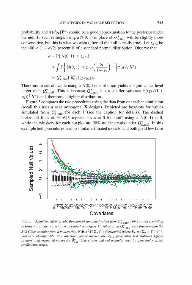
Figure 3 compares the two procedures using the data from our earlier simulation(recall this uses a near orthogonal X design). Depicted are boxplots for valuessimulated from Q∗

k,null for each k (see the caption for details). The dashedhorizontal lines at ±1.645 represent a α = 0.10 cutoff using a N(0,1) null,while the whiskers for each boxplot are 90% null intervals under Q∗

k,null. In thisexample both procedures lead to similar estimated models, and both yield few false

FIG. 3. Adaptive null intervals. Boxplots of simulated values from Q∗k,null, with k sorted according

to largest absolute posterior mean (data from Figure 1). Values from Q∗k,null were drawn within the

SVS Gibbs sampler from a multivariate N(0, σ 2Vtn�nVn) distribution where Vn = (�n + �−1)−1.

Whiskers identify 90% null intervals. Superimposed are Zk,n frequentist test statistics (greensquares) and estimated values for β∗

k,n (blue circles and red triangles used for zero and nonzerocoefficients, resp.).


discoveries. In general, however, we prefer the N(0,1) approach because of itssimplicity and conservativeness. Nevertheless, the Q∗

k,null intervals can always beproduced as part of the analysis. These intervals are valuable because they depictthe variability in the posterior mean under the null but are also adaptive to the truevalue of the coefficient via π(dγk|Y∗).

5.2. The Zcut rule. The preceding argument suggests the use of a thresholdingrule that treats the posterior mean as a N(0,1) test statistic. This method, and theresulting hard shrinkage model estimator, have been referred to as Zcut [Ishwaranand Rao (2000, 2003, 2005)]. Here is its formal definition.

THE ZCUT MODEL ESTIMATOR. Let β∗n = ( β∗

1,n, . . . , β∗K,n)

t be the posteriormean for β from (5). The Zcut model contains all coefficients βk whose posteriormeans satisfy |β∗

k,n| ≥ zα/2. That is,

Zcut := {βk : |β∗k,n| ≥ zα/2}.

Here α > 0 is some fixed value specified by the user. The Zcut estimator for β0 isthe restricted OLS estimator applied to only those coefficients in the Zcut model(all other coefficients are set to zero).

Zcut hard shrinks the posterior mean. Hard shrinkage is important because itreduces the dimension of the model estimator, which is a key to successful subsetselection. Given that the posterior mean is already taking advantage of shrinkage,it is natural to wonder how this translates into performance gains over conventionalhard shrinkage procedures. We compare Zcut theoretically to “OLS-hard,” the hardshrinkage estimator formed from the OLS estimator β

◦n = ( β◦

1,n, . . . , β◦K,n)

t . Hereis its definition:

THE OLS-HARD MODEL ESTIMATOR. The OLS-hard model corresponds tothe model with coefficients βk whose Z-statistics, Zk,n, satisfy |Zk,n| ≥ zα/2,where

Zk,n = n1/2β◦k,n

σn(skk)1/2(12)

and skk is the kth diagonal value from �−1n . That is,

OLS-hard := {βk : |Zk,n| ≥ zα/2}.The OLS-hard estimator for β0 is the restricted OLS estimator using only OLS-hard coefficients.


5.3. Oracle risk performance. If Zcut is going to outperform OLS-hard ingeneral, then it is reasonable to expect it will be better in the fixed hypervariancecase for some appropriately selected γ . Theorem 5, our next result, shows this tobe true in the context of risk performance. We show there exists a value γ = γ 0 thatleads not only to better risk performance, but uniformly better risk performance.Let B0 = {k :βk,0 = 0} be the indices for the zero coefficients of β0. Define

RZ(α) = ∑k∈B0

P{|β∗k,n| ≥ zα/2} + ∑

k∈Bc0

P{|β∗k,n| < zα/2}.

This is the expected number of coefficients misclassified by Zcut for a fixedα-level. This can be thought of as the risk under a zero–one loss function. Themisclassification rate for Zcut is RZ(α)/K . Similarly, define

RO(α) = ∑k∈B0

P{|Zk,n| ≥ zα/2} + ∑k∈Bc

0

P{|Zk,n| < zα/2}

to be the risk for OLS-hard.

THEOREM 5. Assume that the linear regression model (1) holds such thatk0 < K and where εi are i.i.d. N(0, σ 2

0 ). Assume that in (5) β has a N(0,�0)

prior, µ{σ 2 = 1} = 1 and λn = n. Then for each 0 < δ < 1/2 there exists a γ 0such that RZ(α) < RO(α) for all α ∈ [δ,1 − δ].

Theorem 5 shows that Zcut’s risk is uniformly better than the OLS-hard in anyfinite sample setting if γ is set at the oracle value γ 0. Of course, in practice,this oracle value is unknown, which raises the interesting question of whether thesame risk behavior can be achieved by relying on a well-chosen prior for γ . Also,Theorem 5 requires that εi are normally distributed, but can this assumption beremoved?

5.4. Risk performance for continuous bimodal priors. Another way to framethese questions is in terms of the posterior behavior of the hypervariances γk . Thisis because risk performance ultimately boils down to their behavior. One can seethis by carefully inspecting the proof of Theorem 5. There the oracle γ 0 is chosenso that its values are large for the nonzero βk,0 coefficients and small otherwise.Under any prior π ,

β∗k,n = Eπ

(γk

1 + γk

∣∣∣Y∗)Zk,n.

In particular, for the π obtained by fixing γ at γ 0, the posterior mean isshrunk toward zero for the zero coefficients, thus greatly reducing the number ofmisclassifications from this group of variables relative to OLS-hard. Meanwhilefor the nonzero coefficients, β∗

k,n is approximately equal to Zk,n, so the risk from


this group of variables is the same for both procedures, and, therefore, Zcut’s risk issmaller overall. Notice that choosing γ 0 in this fashion also leads to what we havebeen calling selective shrinkage. So good risk performance follows from selectiveshrinkage, which ultimately is a statement about the posterior behavior of γk . Thismotivates the following theorem.

THEOREM 6. Assume in (1) that condition (D2) holds and εi are independentsuch that E(εi) = 0, E(ε2

i ) = σ 20 and E(ε4

i ) ≤ M for some M < ∞. Suppose in (5)that µ{σ 2 = 1} = 1 and λn = n.

(a) If the support for π contains a set [η0,∞)K for some finite constant η0 ≥ 0,then, for each small δ > 0,

πn

({γ :

γk

1 + γk

> 1 − δ

}∣∣∣Y∗)

p→ 1 if βk,0 �= 0,

where πn(·|Y∗) is the posterior measure for γ .(b) Let f ∗

k (·|w) denote the posterior density for γk given w. If π is thecontinuous bimodal prior specified by (4), then

f ∗k (u|w) ∝ exp

(u

2(1 + u)ξ2k,n

)(1 + u)−1/2((1 − w)g0(u) + wg1(u)

),(13)

where g0(u) = v0u−2g(v0u

−1), g1(u) = u−2g(u−1),

g(u) = aa12

(a1 − 1)!ua1−1 exp(−a2u),

and ξk,n = σ−1n n−1/2∑n

i=1 xi,kYi . Note that if βk,0 = 0, then ξk,nd� N(0,1).

Part (a) of Theorem 6 shows why continuity for π is needed for good riskperformance. To be able to selectively shrink coefficients, the posterior mustconcentrate on arbitrarily large values for the hypervariance when the coefficientis truly nonzero. Part (a) shows this holds asymptotically as long as π hasan appropriate support. A continuous prior meets this requirement. Selectiveshrinkage also requires small hypervariances for the zero coefficients, which iswhat part (b) asserts happens with a continuous bimodal prior. Note importantlythat this is a finite sample result and is distribution free. The expression (13) showsthat the posterior density for γk (conditional on w) is bimodal. Indeed, except forthe leading term

exp(

u

2(1 + u)ξ2k,n

),(14)

which reflects the effect on the prior due to the data, the posterior density is nearlyidentical to the prior. What (14) does is to adjust the amount of probability at theslab in the prior (cf. Figure 2) using the value of ξ2

k,n. As indicated in part (b), if


the coefficient is truly zero, then ξ2k,n will have an approximate χ2-distribution,

so this should introduce a relatively small adjustment. Notice this also implies thatthe effect of the prior does not vanish asymptotically for zero coefficients. This is akey aspect of using a rescaled spike and slab model. Morever, because the posteriorfor γk will be similar to the prior when βk,0 = 0, it will concentrate near zero, andhence the posterior mean will be biased and shrunken toward zero relative to thefrequentist Z-test.

On the other hand, if the coefficient is nonzero, then (14) becomes exponentiallylarge and most of the mass of the density shifts to larger hypervariances. This, ofcourse, matches up with part (a) of the theorem. Figure 4 shows how the posteriorcumulative distribution function varies in terms of ξ2

k,n. Even for fairly large valuesof ξ2

k,n (e.g., from the 75th percentile of a χ2-distribution), the distribution functionconverges to one rapidly for small hypervariances. This shows that the posteriorwill concentrate on small hypervariances unless ξ2

k,n is abnormally large.Figure 5 shows how the hypervariances might vary in a real example. We

have plotted the posterior means β∗k,n for the Breiman simulation of Figure 1

against E((γk/(1 + γk))2|Y∗) (the variance of Q∗

k,null). This shows quite clearlythe posterior’s ability to adaptively estimate the hypervariances for selectiveshrinkage. Figure 6 shows how this selective shrinkage capability is translated

FIG. 4. Posterior cumulative distribution function for γk conditional on w (hyperparameters equalto those in Figure 2 and w = 0.3). Curves from top to bottom are derived by setting ξ2

k,n at the

25,50,75 and 90th percentiles for a χ2-distribution with one degree of freedom. Standardizedhypervariance axis defined as γk/(1 + γk).


FIG. 5. Posterior means β∗k,n versus variances E((γk/(1 + γk))

2|Y∗) of Q∗k,null from simulation

used in Figure 1. Triangles in red are nonzero coefficients.

FIG. 6. Total number of misclassified coefficients from simulation used in Figure 1. Observe howZcut’s total misclassification is less than OLS-hard’s over a range of cutoff values zα/2.


into risk performance. As seen, Zcut’s misclassification performance is uniformlybetter than OLS-hard over a wide range of cut-off values, exactly as our theorysuggests.

REMARK 5. The assumption in Theorems 5 and 6 that µ{σ 2 = 1} = 1 isnot typical in practice. As discussed, it is beneficial to assume that σ 2 has acontinuous prior to allow adaptive penalization. Nevertheless, Theorem 5 showseven if σ 2 = 1, thus forgoing the extra benefits of finite sample adaptation, the totalrisk for Zcut with an appropriately fixed γ 0 is still uniformly better than OLS-hard.The same argument could be made for Theorem 6. That is, from a theoretical pointof view, it is not restrictive to assume a fixed σ 2.

5.5. Complexity recovery. We further motivate Zcut by showing that itconsistently estimates the true model under a threshold value that is allowed tochange with n. Let

M0 = (I{β1,0 �= 0}, . . . , I{βK,0 �= 0})tbe the K-dimensional binary vector recording which coordinates of β0 are nonzero[I(·) denotes the indicator function]. By consistent estimation of the true model,

we mean the existence of an estimator Mn such that Mnp→ M0. We show that

such an estimator can be constructed from β∗n. Let

Mn(C) = (I{|β∗1,n| ≥ C}, . . . , I{|β∗

K,n| ≥ C})t .The Zcut estimator corresponds to setting C = zα/2. The next theorem showswe can consistently recover M0 by letting C converge to ∞ at any rate slowerthan

√n.

THEOREM 7. Assume that the priors π and µ in (5) are chosen so thatπ{γk ≥ η0} = 1 for some η0 > 0 for each k = 1, . . . ,K and that µ{σ 2 ≤ s2

0} = 1for some 0 < s2

0 < ∞. Let Mn = Mn(Cn), where Cn → ∞ is any positiveincreasing sequence such that Cn/

√n → 0. Assume that the linear regression

model (1) holds where εi are independent such that E(εi) = 0, E(ε2i ) = σ 2

0 and

E(ε4i ) ≤ M for some M < ∞. If (D2) holds and λn = n, then Mn

p→ M0.

An immediate consequence of Theorem 7 is that the true model complexity k0can be estimated consistently. By the continuous mapping theorem, we obtain thefollowing:

COROLLARY 1. Let Mn = (M1,n, . . . ,MK,n)t and let kn =∑K

k=1 I{Mk,n �= 0} be the number of nonzero coordinates of Mn. Then, under the

conditions of Theorem 7, knp→ k0.


6. The effects of model uncertainty. In this section we prove an asymptoticcomplexity result for a specialized type of forward stepwise model selectionprocedure. This forward stepwise method is a modification of a backwardstepwise procedure introduced by Pötscher (1991) and discussed recently in Leeband Pötscher (2003). We show in orthogonal settings that if the coordinatesof β0 are perfectly ordered a priori, then the forward stepwise procedure leadsto improved complexity recovery relative to the OLS-hard. Interestingly, thebackward stepwise procedure has the worst performance of all three methods(Theorem 8 of Section 6.3). This result can be used as an empirical tool forassessing a procedure’s ability to reduce model uncertainty. If a model selectionprocedure is effectively reducing model uncertainty, then it should produce anaccurate ranking of coefficients in finite samples. Consequently, the forwardstepwise procedure based on this data based ranking should perform better thanOLS-hard. This provides an indirect way to confirm a procedure’s ability to reducemodel uncertainty.

REMARK 6. The idea of pre-ranking covariates and then selecting models hasbecome a well established technique in the literature. As mentioned, this idea wasused by Pötscher (1991) and Leeb and Pötscher (2003), but also appears in Zhang(1992), Zheng and Lo (1995, 1997), Rao and Wu (1989) and Ishwaran (2004).

We use this strategy to assess the performance of a rescaled spike and slabmodel. For a data based ordering of β , we use the absolute posterior means |β∗

k,n|.The first coordinate of β corresponds to the largest absolute posterior value, thesecond coordinate to the second largest value, and so forth. The data based forwardstepwise procedure using this ranking is termed “svsForwd.” Section 6.2 providesa formal description. In Section 8 we use simulations to systematically comparethe performance of svsForwd to OLS-hard as an indirect way to confirm SVS’sability to reduce model uncertainty. Figure 7 provides some preliminary evidenceof this capability. There we have compared a ranking of β using the posterior meanagainst an OLS ordering using |Zk,n|. Figure 7 is based on the simulation presentedin Figure 1.

We note that it is possible to consistently estimate the order of the β0coordinates using the posterior mean. Let Uk,n be the kth largest value from theset {|β∗

k,n| :k = 1, . . . ,K}. That is, U1,n ≥ U2,n ≥ · · · ≥ UK,n. Let

M(n) = (I{U1,n ≥ Cn}, . . . , I{UK,n ≥ Cn})t ,where Cn is a positive sequence satisfying Cn → ∞ and Cn/

√n → 0. By

inspection of the proof of Theorem 7, Corollary 2 can be shown.

COROLLARY 2. Under the conditions of Theorem 7, M(n)p→ (1, . . . ,

1,0tK−k0

)t .


FIG. 7. (a) True rank of a coefficient versus estimated rank using posterior means (circles) and OLS(squares). The lower the rank, the larger the absolute value of the coefficient. Data from Breimansimulation of Figure 1 (only nonzero coefficients shown). (b) Same plot as (a) but with true ranksaveraged to adjust for ties in true coefficient values (simulation used four unique nonzero coefficientvalues). Dashed line connects values for true average rank. Note the higher variability in OLS,especially for intermediate coefficients.


6.1. Backward model selection. We begin by reviewing the backward step-wise procedure of Pötscher (1991). For notational ease, we avoid subscripts of n

as much as possible. We assume the coordinates of β0 have been ordered, so thatthe first k0 coordinates are nonzero. That is,

β0 = (β1,0, . . . , βk0,0,0t

K−k0

)t,

where 0K−k0 is the (K − k0)-dimensional zero vector. We assume the designmatrix X has been suitably recoded as well. Let X[k] be the n × k design matrixformed from the first k columns of the re-ordered X. Let

β◦[k] = ( β◦

1 [k], . . . , β◦k [k])t

= (X[k]tX[k])−1X[k]tYbe the restricted OLS estimator using only the first k variables. To test whether thekth coefficient βk is zero, define the test statistic

Zk,n = n1/2β◦k [k]

σn(skk[k])1/2 ,(15)

where skk[k] is the kth diagonal value from (X[k]tX[k]/n)−1. Let α1, . . . , αK

be a sequence of fixed positive α-significance values for the Zk,n test statistics.Estimate the true complexity k0 by the estimator kB , where

kB = max{k : |Zk,n| ≥ zαk/2, k = 0, . . . ,K

}.

To ensure that kB is well defined, take Z0,n = 0 and zα0/2 = 0.Observe if kB = k, then Zk,n is the first test starting from k = K and going

backward to k = 0 satisfying |Zk,n| ≥ zαk/2 and |Zj,n| < zαj /2 for j = k +1, . . . ,K . This corresponds to accepting the event {β :βk+1 = 0, . . . , βK = 0}, butrejecting {β :βk = 0, . . . , βK = 0}. The post-model selection estimator for β isdefined as

βB = 0KI{kB = 0} +K∑

k=1

( β◦[k]t ,0t

K−k)tI{kB = k}.

It should be clear that the estimators kB and βB are derived from a backwardstepwise mechanism.

REMARK 7. Observe that Zk,n uses σ 2n , the estimate for σ 2

0 based on the fullmodel, rather than an estimate based on the first k variables, and so, in this way,is different from a conventional stepwise procedure. The latter estimates are onlyunbiased if k ≥ k0 and can perform quite badly otherwise.


REMARK 8. At first glance it seems the backward procedure requires K

regression analyses to compute β◦[k] for each k. This would be expensive for

large K , requiring a computational effort of O(∑K

k=1 k3). In fact, the wholeprocedure can be reduced to the problem of finding an orthogonal decompositionof the X matrix, an O(K3) operation. This idea rests on the following observationsimplicit in Lemma A.1 of Leeb and Pötscher (2003). Let

P⊥k = I − X[k](X[k]tX[k])−1X[k]t

be the projection onto the orthogonal complement of the linear space spannedby X[k]. Let x(k) denote the kth column vector of X (thus X[k] = [x(1), . . . ,x(k)]).Define

u1 = x(1) and uk = P⊥k−1x(k) for k = 2, . . . ,K.

One can show that

β◦k [k] = (ut

kuk)−1ut

kY, k = 1, . . . ,K.

Consequently, the backward procedure is equivalent to finding an orthogonaldecomposition of X. (Note that this argument shows β◦

1 [1], . . . , β◦K [K] are

mutually uncorrelated if εi are independent, E(εi) = 0 and E(εi) = σ 20 . See

Lemma A.1 of Leeb and Pötscher (2003). This will be important in the proof ofTheorem 8.)

6.2. Forward model selection. A forward stepwise procedure and its associ-ated post-model selection estimator for β0 can be defined in an analogous way.Define

kF = min{k − 1 : |Zk,n| < zαk/2, k = 1, . . . ,K + 1

},(16)

where ZK+1,n = 0 and αK+1 = 0 are chosen to ensure a well-defined procedure.Observe if kF = k − 1, then Zk,n is the first test statistic such that |Zk,n| < zαk/2,while |Zj,n| ≥ zαj /2 for j = 1, . . . , k − 1. This corresponds to accepting the event

{β :β1 �= 0, . . . , βk−1 �= 0}, but rejecting {β :β1 �= 0, . . . , βk �= 0}. Note that kF = 0if |Z1,n| < zα1/2. The post-model selection estimator for β0 is

βF = 0KI{kF = 0} +K∑

k=1

( β◦[k]t ,0t

K−k)tI{kF = k}.(17)

The data based version of forward stepwise, svsForwd, mentioned earlier is definedas follows:

THE SVSFORWD MODEL ESTIMATOR. Re-order the coordinates of β (and thecolumns of the design matrix X) using the absolute posterior means β∗

k,n from (5).

If kF ≥ 1, the svsForwd model is defined as

svsForwd := {βk :k = 1, . . . , kF };


otherwise, if kF = 0, let svsForwd be the null model. Define the svsForwd post-model selection estimator for β0 as in (17).

6.3. Complexity recovery. The following theorem identifies the limiting dis-tribution for kB and kF . It also considers OLS-hard. Let kO denote the OLS-hardcomplexity estimator (i.e., kO equals the number of parameters in OLS-hard).Part (a) of the following theorem is related to Lemma 4 of Pötscher (1991).

THEOREM 8. Assume that (D1)–(D4) hold for (1), where εi are independentsuch that E(εi) = 0, E(ε2

i ) = σ 20 and E(ε4

i ) ≤ M for some M < ∞. Let kB ,kF and kO denote the limits for kB , kF and kO , respectively, as n → ∞. For1 ≤ k ≤ K ,

(a) P{kB = k} = 0 × I{k < k0} + (1 − αk0+1

) · · · (1 − αK)I{k = k0}+ αk(1 − αk+1) · · · (1 − αK)I{k > k0}.

Moreover, when X has an orthogonal design (i.e., �n = �0 = I),

(b) P{kF = k} = 0 × I{k < k0} + (1 − αk0+1

)I{k = k0}

+ (1 − αk+1)αk0+1 · · ·αkI{k > k0}.(c) P{kO = k} = 0 × I{k < k0}

+ P{Bk0+1 + · · · + BK = k − k0

}I{k ≥ k0},

where αK+1 = 0 in (b) and Bk are independent Bernoulli(αk) random variablesfor k = k0 + 1, . . . ,K .

REMARK 9. Although the result (b) requires an assumption of orthogonality,this restriction can be removed. See equation (38) of Corollary 4.5 from Leeb andPötscher (2003).

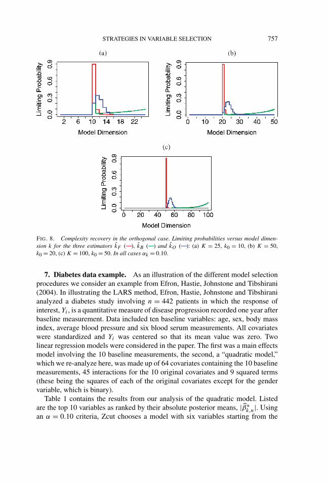
Theorem 8 shows that forward stepwise is the best procedure in orthogonaldesigns. Suppose that αk = α > 0 for each k. Then the limiting probability ofcorrectly estimating k0 is P{kF = k0} = (1 − α) for forward stepwise, whilefor OLS-hard and backward stepwise, it is (1 − α)K−k0 . Notice if K − k0 islarge, this last probability is approximated by exp(−(K − k0)α), which becomesexponentially small as K increases. Simply put, the OLS-hard and backwardstepwise methods are prone to overfitting. Figure 8 illustrates how the limitingprobabilities vary under various choices for K and k0 (all figures computed withα = 0.10). One can clearly see the superiority of the forward procedure, especiallyas K increases.


FIG. 8. Complexity recovery in the orthogonal case. Limiting probabilities versus model dimen-sion k for the three estimators kF ( ), kB ( ) and kO ( ): (a) K = 25, k0 = 10, (b) K = 50,k0 = 20, (c) K = 100, k0 = 50. In all cases αk = 0.10.

7. Diabetes data example. As an illustration of the different model selectionprocedures we consider an example from Efron, Hastie, Johnstone and Tibshirani(2004). In illustrating the LARS method, Efron, Hastie, Johnstone and Tibshiranianalyzed a diabetes study involving n = 442 patients in which the response ofinterest, Yi , is a quantitative measure of disease progression recorded one year afterbaseline measurement. Data included ten baseline variables: age, sex, body massindex, average blood pressure and six blood serum measurements. All covariateswere standardized and Yi was centered so that its mean value was zero. Twolinear regression models were considered in the paper. The first was a main effectsmodel involving the 10 baseline measurements, the second, a “quadratic model,”which we re-analyze here, was made up of 64 covariates containing the 10 baselinemeasurements, 45 interactions for the 10 original covariates and 9 squared terms(these being the squares of each of the original covariates except for the gendervariable, which is binary).

Table 1 contains the results from our analysis of the quadratic model. Listedare the top 10 variables as ranked by their absolute posterior means, |β∗

k,n|. Usingan α = 0.10 criteria, Zcut chooses a model with six variables starting from the


top variable “bmi” (body mass index) and ending with “age.sex” (the age–sexinteraction effect). The seventh variable, “bmi.map” (the interaction of body massindex and map, a blood pressure measurement), is borderline significant. Table 1also reports results using OLS-hard, svsForwd and a new procedure, “OLSForwd”(all using an α = 0.10 value). OLSForwd is the direct analogue of svsForwd, butorders β using Z-statistics Zk,n in place of the posterior mean. For all proceduresthe values in Table 1 are Z-statistics (12) derived from the restricted OLS for theselected model. This was done to allow direct comparison to the posterior meanvalues recorded in column 2.

Table 1 shows that the OLS-hard model differs significantly from Zcut. Itexcludes both “ltg” and “hdl” (blood serum measurements), both of which havelarge posterior mean values. We are not confident in the OLS-hard and suspectit is missing true signal here. The same comment applies to OLSForwd, whichhas produced the same model as OLS-hard. Note how svsForwd, the counterpartfor OLSForwd, agrees closely with Zcut (it disagrees only on bmi.map, which isborderline significant). We believe the SVS models are more accurate than the OLSones. In the next section we more systematically study the differences between thefour procedures.

REMARK 10. Figure 9 displays the posterior density for σ 2. Note how theposterior is concentrated near one. This is typical of what we see in practice.

8. Breiman simulations. We used simulations to more systematically studyperformance. These followed the recipe given in Breiman (1992). Specifically,data were generated by taking εi to be i.i.d. N(0,1) variables, while covariates xi

TABLE 1Top 10 variables from diabetes data (ranking based on absolute posteriormeans |β∗

k,n|). Entries for model selection procedures are Z-statistics (12)derived from the restricted OLS for the selected model

Variable β∗k,n Zcut OLS-hard svsForwd OLSForwd

1 bmi 9.54 8.29 13.70 8.15 13.702 ltg 9.25 7.68 0.00 7.82 0.003 map 5.64 5.39 7.06 4.99 7.064 hdl −4.37 −4.20 0.00 −4.31 0.005 sex −3.38 −4.03 −1.95 −4.02 −1.956 age.sex 2.43 3.58 3.19 3.47 3.197 bmi.map 1.61 0.00 2.56 3.28 2.568 glu.2 0.84 0.00 0.00 0.00 0.009 bmi.2 0.46 0.00 0.00 0.00 0.00

10 tc.tch −0.44 0.00 0.00 0.00 0.00


FIG. 9. Posterior density for σ 2 from diabetes analysis.

were simulated independently from a multivariate normal distribution suchthat E(xi ) = 0 and E(xi,j xi,k) = ρ|j−k|, where 0 < ρ < 1 was a correlationparameter. We considered two settings for ρ: (i) an uncorrelated design, ρ = 0;(ii) a correlated design, ρ = 0.90. For each ρ setting we also considered twodifferent sample size and model dimension configurations: (A) n = 200 andK = 100; (B) n = 800 and K = 400. Note that our illustrative example of Figure 1corresponds to the Monte Carlo experiment (B) with ρ = 0.

In the higher-dimensional simulations (B), the nonzero βk,0 coefficients were in15 clusters of 7 adjacent variables centered at every 25th variable. For example,for the variables clustered around the 25th variable, the coefficient values weregiven by β25+j,0 = |h − j |1.25 for |j | < h, where h = 4. The other 14 clusterswere defined similarly. All other coefficients were set to zero. This gave a totalof 105 nonzero values and 295 zero values. Coefficient values were adjusted bymultiplying by a common constant to make the theoretical R2 value equal to 0.75[see Breiman (1992) for a discussion of this point].

Simulations (B) reflect a regression framework with a large number of zerocoefficients. In contrast, simulations (A) were designed to represent a regressionmodel with many weakly informative covariates. For (A), nonzero βk,0 coefficientswere grouped into 9 clusters each of size 5 centered at every 10th variable. Each ofthe 45 nonzero coefficients was set to the same value. Coefficient values were thenadjusted by multiplying by a common constant to make the theoretical R2 valueequal to 0.75. This ensured that the overall signal to noise ratio was the same as(B), but with each coefficient having less explanatory power.

Simulations were repeated 100 times independently for each of the fourexperiments. Results are recorded in Table 2 for each of the procedures Zcut,


svsForwd, OLS-hard and OLSForwd (all using an α = 0.10 value). Table 2 recordswhat we call “TotalMiss,” “FDR” and “FNR.” The TotalMiss is the total number ofmisclassified variables, that is, the total number of falsely identified nonzero βk,0coefficients and falsely identified zero coefficients. This is an unbiased estimatorfor the risk discussed in Theorem 5. The FDR and FNR are the false discovery andfalse nondiscovery rates defined as the false positive and false negative rates forthose coefficients identified as nonzero and zero, respectively. The TotalMiss, FDRand FNR values reported are the averaged values from the 100 simulations. Alsorecorded is k, the average number of variables selected by a procedure. Table 2 alsoincludes the performance value “Perf,” a measure of prediction accuracy, definedas

Perf = 1 − ‖Xβ − Xβ0‖2

‖Xβ0‖2 ,

where β is the estimator for β0. So Perf equals zero when β = 0 and equals onewhen β = β0. The value for Perf was again averaged over the 100 simulations.

REMARK 11. Given the high dimensionality of the simulations, both svs-Forwd and OLSForwd often stopped early and produced models that were muchtoo small. To compensate, we slightly altered their definitions. For svsForwd, wemodified the definition of kF [cf. (16)] to

kF = min{k − 1 : |Zk,n| < zαk/2 and |β∗

k,n| ≤ C,k = 1, . . . ,K + 1},

where C = 3. In this way, svsForwd stops the first time the null hypothesis is notrejected and if the absolute posterior mean is no longer a large value. The definition

TABLE 2Breiman simulations

ρ = 0 (uncorrelated X) ρ = 0.9 (correlated X)

k Perf TotalMiss FDR FNR k Perf TotalMiss FDR FNR

(A) Moderate number of covariates with few (55%) that are zero(n = 200, K = 100 and 55 zero βk,0).

Zcut 41.44 0.815 11.99 0.097 0.129 10.06 0.853 38.49 0.167 0.408svsForwd 34.02 0.753 15.09 0.054 0.191 8.31 0.826 39.39 0.156 0.415OLS-hard 41.99 0.791 14.06 0.128 0.145 11.08 0.707 45.31 0.496 0.446OLSForwd 26.90 0.612 20.92 0.042 0.258 5.96 0.574 44.64 0.459 0.445

(B) Large number of covariates with many (74%) that are zero(n = 800, K = 400 and 295 zero βk,0).

Zcut 75.96 0.903 39.62 0.068 0.106 36.67 0.953 72.61 0.055 0.194svsForwd 86.81 0.904 41.19 0.130 0.095 24.42 0.926 81.90 0.025 0.216OLS-hard 106.74 0.883 58.54 0.279 0.097 45.41 0.706 121.37 0.676 0.255OLSForwd 61.09 0.846 49.87 0.046 0.138 9.14 0.303 106.48 0.590 0.259


for OLSForwd was altered in similar fashion, but using Zk,n in place of β∗k,n.

8.1. Results. The simulations revealed several interesting patterns, summa-rized as follows:

1. Zcut beats OLS-hard across all performance categories. It maintains low risk,has small FDR values and has good prediction error performance in boththe near-orthogonal (uncorrelated) and nonorthogonal (correlated) X cases.Performance differences between Zcut and OLS-hard become more appreciablein the near-orthogonal simulation (B) involving many zero coefficients, becausethis is when the effect of selective shrinkage is most pronounced. For example,the OLS-hard misclassifies about 19 coefficients more on average, and has aFDR more than 4 times larger than Zcut’s. Large gains are also seen in thecorrelated case (B). There, the OLS-hard misclassifies over 48 more coefficientson average than Zcut and its FDR is more than 12 times higher.

2. It is immediately clear upon comparing svsForwd to OLSForwd that SVS iscapable of some serious model averaging. These two procedures differ only inthe way they rank coefficients, so the disparity in their two performances isclear evidence of SVS’s ability to model average.

3. In the ρ = 0 simulations, svsForwd is roughly the same as OLS-hard insimulation (A) and significantly better in simulation (B). In the correlatedsetting, svsForwd is significantly better. Thus, overall svsForwd is as good, andin most cases significantly better, than OLS-hard. This suggests that svsForwdis starting to tap into the oracle property forward stepwise has relative to OLS-hard and provides indirect evidence that SVS is capable of reducing modeluncertainty in finite samples.

4. It is interesting to note how badly OLSForwd performs relative to OLS-hardin simulation (A) when ρ = 0. In orthogonal designs, OLSForwd is equivalentto OLS-hard, but the ρ = 0 design is only near-orthogonal. With only a slightdeparture from orthogonality, we see the importance of a reliable ranking forthe coordinates of β . Note that this effect is less pronounced in simulation (B)because of the larger sample size. This is because XtX/n

a.s.→ I as n → ∞, sosimulation (B) should be closer to orthogonality.

5. While our theory does not cover Zcut’s performance in correlated settings, it isinteresting to note how well it does in the ρ = 0.9 simulations relative to OLS-hard. The explanation for its success here, however, is probably different fromthat for the orthogonal setting. For example, it is possible that its performancegains may be mostly due to the use of generalized ridge estimators. As iswell known, such estimators are much more stable than OLS in multicollinearsettings. We should also note that while Zcut is better than OLS-hard here, itsperformance relative to the orthogonal simulations is noticeably worse. This isnot unexpected though. Correlation has the effect of reducing the dimensionof the problem. So performance measurements like TotalMiss and FDR willnaturally be less favorable.


APPENDIX: PROOFS

PROOF OF THEOREM 2. We start by establishing that β◦n is consistent, which

is part of the conclusion of Theorem 2. First observe that

β◦n = n−1�−1

n XtY = β0 + �n,

where �n = �−1n Xtε/n and ε = (ε1, . . . , εn)

t . From E(�n) = 0 and Var(�n) =σ 2

0 �−1n /n, it is clear that β

◦n

p→ β0. Next, a little bit of rearrangement shows that

θ∗n(γ , σ 2) = (

I − (σ−2λ−1n XtX + �−1)−1�−1)β◦

n.

Consequently,

θ∗n = β

◦n −

∫(σ−2λ−1

n XtX + �−1)−1�−1β◦n (π × µ)(dγ , dσ 2|Y∗)

= β◦n − λ∗

n

∫σ 2V−1

n �−1β◦n(π × µ)(dγ , dσ 2|Y∗),

where λ∗n = λn/n and Vn = �n + σ 2λ∗

n�−1. By the Jordan decomposition the-

orem, we can write Vn =∑Kk=1 ek,nvk,nvt

k,n, where {vk,n} is a set of orthonormaleigenvectors with eigenvalues {ek,n}. For convenience, assume that the eigenvalueshave been ordered so that e1,n ≤ · · · ≤ eK,n. The assumption that �n → �0, where�0 is positive definite, ensures that the minimum eigenvalue for �n is larger thansome e0 > 0 for sufficiently large n. Therefore, if n is large enough,

e1,n ≥ e0 + σ 2λ∗n min

kγ −1k ≥ e0 > 0.

Notice that

‖V−1n �−1β

◦n‖2 =

K∑k=1

e−2k,n(v

tk,n�

−1β◦n)

2 ≤ e−20 ‖β◦

n‖2K∑

k=1

γ −2k .

Thus, since γk ≥ η0 over the support of π , and σ 2 ≤ s20 over the support of µ,∥∥∥∥∫ σ 2V−1

n �−1β◦n (π × µ)(dγ , dσ 2|Y∗)

∥∥∥∥≤ e−1

0 ‖β◦n‖(

K∑k=1

∫σ 4γ −2

k (π × µ)(dγ , dσ 2|Y∗))1/2

≤ K1/2s20

η0e0‖β◦

n‖.

Deduce that θ∗n = β

◦n + Op(λ∗

n)p→ β0. �

Before proving Theorem 3, we state a lemma. This will also be useful in theproofs of some later theorems.


LEMMA A.1. Assume that for each n, εn1, . . . , εnn are independent randomvariables such that E(εni) = 0, E(ε2

ni) = σ 20 and E(ε4

ni) ≤ M for some finite M .If (D1)–(D4) hold, then

n−1/2Xtεn = n−1/2n∑

i=1

εnixid� N(0, σ 2

0 �0),(18)

where εn = (εn1, . . . , εnn)t .

PROOF. Let Sn =∑ni=1 εnixt

i/√

n, where ∈ RK is some arbitrary nonzero

vector. Let s2n = σ 2

0 t�n and define ζni = n−1/2εnixti/sn. Then, Sn/sn =∑n

i=1 ζni , where ζni are independent random variables such that E(ζni) = 0 and∑ni=1 E(ζ 2

ni) = 1. To prove (18), we will verify the Lindeberg conditionn∑

i=1

E(ζ 2niI{|ζni | ≥ δ}) → 0 for each δ > 0,

where I(·) denotes the indicator function. This will show that Sn/snd� N(0,1),

which by the Cramér–Wold device implies (18) because s2n → σ 2

0 t�0. Observethat

E(ζ 2niI{|ζni | > δ}) = (xt

i)2

ns2n

E(ε2niI{|εni | ≥ rnisnδ}),

where rni = √n/|xt

i|. By the Cauchy–Schwarz inequality and the assumption ofa bounded fourth moment for εni ,

E(ε2niI{|εni | ≥ rnisnδ}) ≤ (

E(ε4ni)P{|εni | ≥ rnisnδ})1/2 ≤ M1/2σ0

rnisnδ.

Bound rni below by

rni ≥ rn :=(

max1≤i≤n

|xti|/

√n

)−1

.

Notice that rn → ∞ by the assumption that maxi ‖xi‖/√n → 0. Substituting thebound for rni , and since (xt

i)2 sums to ns2

n/σ 20 , and s2

n remains bounded awayfrom zero since s2

n → σ 20 t�0,

n∑i=1

E(ζ 2niI{|ζni | > δ}) ≤ M1/2

σ0rnsnδ→ 0.

�

PROOF OF THEOREM 3. Let φ(·|m,τ 2) denote a normal density withmean m and variance τ 2. By dividing the numerator and denominator byn−K/2∏n

i=1 φ(Y ∗ni |xt

iβ0, n), one can show that

νn(S(β1,C/√

n )|Y∗n)

νn(S(β0,C/√

n )|Y∗n)

= nK/2 ∫I{β ∈ S(β1,C/

√n )}Ln(β) ν(dβ)

nK/2∫

I{β ∈ S(β0,C/√

n )}Ln(β) ν(dβ),(19)


where

log(Ln(β)

)= −12(β − β0)

t�n(β − β0) + n−1/2n∑

i=1

εnixti (β − β0).

Consider the denominator in (19). By making the change of variables from β tou = √

n(β − β0), we can rewrite this as∫I{u ∈ S(0,C)}Ln0(u)f (β0 + n−1/2u) du,(20)

where log(Ln0(u)) = gn(u) + O(1/n) and gn(u) =∑ni=1 εnixt

iu/n. The O(1/n)

term corresponds to ut�nu/n and is uniform over u ∈ S(0,C). Observe that, foreach δ > 0,

P{|gn(u)| ≥ δ} ≤ 1

δ2n2

n∑i=1

E(εnixtiu)2 ≤ C2

δ2n2

n∑i=1

‖xi‖2 = o(1),

where the last inequality on the right-hand side follows from the Cauchy–Schwarzinequality and from the assumption that maxi ‖xi‖/√n = o(1). Therefore,

gn(u)p→ 0 uniformly over u ∈ S(0,C). Because f is continuous [and keeping

in mind it remains positive and bounded over S(0,C)], deduce that the log of (20)converges in probability to

log(f (β0)

)+ log(∫

I{u ∈ S(0,C)}du).(21)

Meanwhile, for the numerator in (19), make the change of variables from β tou = √

n(β − β1) to rewrite this as∫I{u ∈ S(0,C)}Ln1(u)f (β1 + n−1/2u) du,(22)

where

log(Ln1(u)

)= −12(β1 − β0)

t�0(β1 − β0)

+ n−1/2n∑

i=1

εnixti (β1 − β0) + gn(u) + o(1)

uniformly over u ∈ S(0,C). Consider the second term on the right-hand side ofthe last expression. Set = β1 − β0. By Lemma A.1, since σ 2

0 = 1, it follows that

n−1/2n∑

i=1

εnixti

d� N(0,t�0).

Now extract the expressions not depending upon u outside the integral in (22), take

logs and use gn(u)p→ 0 uniformly over u ∈ S(0,C) to deduce that the log of (22)


converges in distribution to

−12(β1 − β0)

t�0(β1 − β0)

+ (β1 − β0)tZ + log

(f (β1)

)+ log(∫

I{u ∈ S(0,C)}du).

(23)

To complete the proof, take the difference of (23) and (21) and note thecancellation of the logs of

∫I{u ∈ S(0,C)}du. �

PROOF OF THEOREM 4. First note that

β∗nn(γ 0) = (XtX+n�−1

0 )−1XtY∗n = (�0 +�−1

0 )−1�0β0 +n−1/2V−1n Xtεn+o(1),

where Vn = �n + �−10 . The o(1) term on the right-hand side is due to �n → �0.

Also, by Lemma A.1, the second term on the right-hand side converges indistribution to (�0 + �−1

0 )−1Z, where Z has a N(0,�0) distribution. Deduce that

β∗nn(γ 0)

d� Q(·|γ 0). �

PROOF OF THEOREM 5. A little algebra (keeping in mind �n = I) showsβ

∗n = √

n(I + �−10 )−1β

◦n/σn. Hence, recalling the definition (12) for Zk,n,

β∗k,n = dk,0 × n1/2β◦

k,n

σn

= dk,0Zk,n,

where dk,0 = γk,0/(1+γk,0) and the last equality holds because skk = 1. Under theassumption of normality,

√nβ◦

k,n has a N(mk,n, σ20 ) distribution, where mk,n =√

nβk,0. Choose γ 0 such that dk,0 = δ1 for each k ∈ B0 and dk,0 = δ2 for eachk ∈ Bc

0, where 0 < δ1, δ2 < 1 are values to be specified. Therefore,

RO(α) − RZ(α)

= (K − k0)(P{|N(0, σ 2

0 )| ≥ σnzα/2} − P{|N(0, σ 20 )| ≥ δ−1

1 σnzα/2})+ ∑

k∈Bc0

(P{|N(mk,n, σ

20 )| < σnzα/2} − P{|N(mk,n, σ

20 )| < δ−1

2 σnzα/2}),where the P-distributions on the right-hand side correspond to the joint distributionfor a normal random variable and the distribution for σn, where σ 2

n /σ 20 has an

independent χ2-distribution with n − K degrees of freedom. It is clear that thesum on the right-hand side can be made arbitrarily close to zero, uniformly forα ∈ [δ,1 − δ], by choosing δ2 close to one, while the first term on the right-handside remains positive and uniformly bounded away from zero over α ∈ [δ,1 − δ]whatever the choice for δ1. Thus, for a suitably chosen δ2, RO(α) − RZ(α) > 0for each α ∈ [δ,1 − δ]. �


PROOF OF THEOREM 6. Choose some j ∈ Bc0. Let Aj = {γ :dj ≤ 1 − δ},

where dj = γj/(1 + γj ). To prove part (a), we show that

πn(Aj |Y∗) =∫Aj

f (Y∗|γ )π(dγ )∫f (Y∗|γ )π(dγ )

p→ 0.

By definition, f (Y∗|γ ) = ∫f (Y∗|β)f (β|γ ) dβ , where

f (Y∗|β)f (β|γ ) = C exp(− 1

2n(Y∗ − Xβ)t (Y∗ − Xβ) − 1

2β t�−1β

)|�|−1/2

and C is a generic constant not depending upon γ . By some straightforwardcalculations that exploit conjugacy and orthogonality,

f (Y∗|γ ) = C exp

(12

K∑k=1

dkξ2k,n

)K∏

k=1

(1 + γk)−1/2,(24)

where (ξ1,n, . . . , ξK,n)t = σ−1

n n−1/2XtY.Let B = {γ : 1 − δk ≤ dk ≤ 1 − δk/2, k = 1, . . . ,K}, where 0 < δk < 1 are small

values that will be specified. Observe that

πn(Aj |Y∗) ≤∫Aj

f (Y∗|γ )π(dγ )∫B f (Y∗|γ )π(dγ )

.

Over the set Aj we have the upper bound

f (Y∗|γ ) ≤ C exp

{12

( ∑k∈B0

ξ2k,n + ∑

k∈Bc0−{j}

ξ2k,n + (1 − δ)ξ2

j,n

)}

because 0 < dk < 1, while over B we have the lower bound

f (Y∗|γ ) ≥ C exp

{1

2

( ∑k∈Bc

0−{j}(1 − δk)ξ

2k,n + (1 − δj )ξ

2j,n

)}K∏

k=1

(2

δk

)−1/2

.

An application of Lemma A.1 (which also applies to nontriangular arrays) shows

(ξ1,n, . . . , ξK,n)t = σ−1

n

(n1/2β0 + Op(1)

).

Therefore,

πn(Aj |Y∗) ≤ exp

{Op(1) + n

2σ 2n

( ∑k∈Bc

0−{j}δkβ

2k,0

+ (δj − δ)β2j,0 + Op

(1/

√n))}π(Aj )

π(B).

(25)


Choose δj < δ. It is clear we can find a set of values {δk :k �= j} chosen smallenough so that ∑

k∈Bc0−{j}

δkβ2k,0 + (δj − δ)β2

j,0 < 0.

This ensures that the expression in the exponent of (25) converges to −∞ inprobability. Note for this result we assume σ 2

n has a nonzero limit (we give a

proof shortly that σ 2n

p→ σ 20 ). Therefore, since π(B) must be strictly positive for

small enough δk > 0 (by our assumptions regarding the support for π ), conclude

from (25) that πn(Aj |Y∗) p→ 0.To prove part (b), let fk(γk|w) denote the density for γk given w. From (4), it is

seen that fk(γk|w) = (1 − w)g0(γk) + wg1(γk). Therefore,

f ∗k (γk|w) ∝ f (Y|γ )fk(γk|w)

∝ exp(1

2dkξ2k,n

)(1 + γk)

−1/2fk(γk|w),

which is the expression (13). Furthermore, by Lemma A.1 deduce that ξk,n

converges to a standard normal if βk,0 = 0 (we are using σ 2n

p→ σ 20 , which still

needs to be proven).To complete the proof, we now show σ 2

n is consistent. For this proof we donot assume orthogonality, only that �n is positive definite (this generality willbe useful for later proofs). Observe that σ 2

n = (εtε − εtHε)/(n − K), whereH = X(XtX)−1Xt . It follows from Chebyshev’s inequality using the moment

assumptions on εi that εtε/(n − K)p→ σ 2

0 , while from Markov’s inequality, foreach δ > 0,

P{εtHε ≥ (n − K)δ} ≤ E(εtHε)

(n − K)δ= Trace(HE(εεt ))

(n − K)δ= Kσ 2

0

(n − K)δ→ 0.

Deduce that σ 2n

p→ σ 20 . �

PROOF OF THEOREM 7. Under the assumption of orthogonality, and usingthe fact that λn = n, it follows that

β∗n(γ , σ 2) = σ−1

n n1/2Dβ0 + σ−1n n−1/2DXtε,

where D is the diagonal matrix diag(d1, . . . , dK) and dk = γk/(γk + σ 2). Takingexpectations with respect to the posterior, deduce that

β∗k,n = σ−1

n n1/2d∗k βk,0 + σ−1

n d∗k ζk,n,(26)

where d∗k = E(dk|Y∗) and ζk,n is the kth coordinate of Xtε/

√n. From Lemma A.1

and σ 2n

p→ σ 20 (proven in Theorem 6), we have σ−1

n Xtε/√

nd� N(0, I). Therefore,

because 0 ≤ d∗k ≤ 1, deduce that the second term on the right-hand side of (26)


is Op(1). Now consider the first term on the right-hand side of (26). Byour assumptions regarding the support of π and µ, we must have d∗

k ≥ η0/

(η0 + s20). Thus, d∗

k remains bounded away from zero in probability. Hence,because Cn/

√n → 0, we have proven that

C−1n |β∗

k,n|p→{

0, if k ∈ B0,∞, otherwise. �

PROOF OF THEOREM 8. As the proof is somewhat lengthy, we first give abrief sketch. The basis for the proof will rely on the following result:

β◦k [k] p→

0, if k0 < k ≤ K ,βk0,0, if k = k0,βk,0 + �k,0, if 1 ≤ k < k0,

(27)

where �k,0 is the kth coordinate of �0[k :k]−1�0[k :−k]β0[−k]. Here β0[−k] =(β0,k+1, . . . , β0,K)t , while �0[k :k] and �0[k :−k] are the k × k and k × (K − k)

matrices associated with �0 which has been partitioned according to

�0 =(

�0[k :k] �0[k :−k]�0[−k :k] �0[−k :−k]

).

First consider what (27) implies when k < k0. Recall the definition (15) for Zk,n.

Using σ 2n

p→ σ 20 (shown in the proof of Theorem 6) and that skk[k] converges to the

kth diagonal value of �0[k :k]−1, a strictly positive value, deduce from the secondlimit of (27) that P{|Zk0,n| ≥ zαk0/2} → 1. Thus, for (a),

P{kB = k} = P{|Zk,n| ≥ zαk/2 and |Zj,n| < zαj/2 for j = k + 1, . . . ,K

}≤ P

{∣∣Zk0,n

∣∣< zαk0/2}→ 0.

For (b), observe that �k,0 = 0 (by our assumption of orthogonality). Thus, whenk ≤ k0, the last two lines of (27) imply that P{|Zk,n| ≥ zαk/2} → 1, and therefore,

P{kF = k − 1} = P{|Zk,n| < zαk/2 and |Zj,n| ≥ zαj /2 for j = 1, . . . , k − 1

}≤ P

{|Zk,n| < zαk/2}→ 0.

Now for (c), due to orthogonality, Zk,n = Zk,n for Zk,n defined by (12). Thus,

P{kO ≥ k0} ≥ P{|Zj,n| ≥ zαj /2 for j = 1, . . . , k0

}→ 1.

Thus, for all three estimators the probability of the event {k < k0} tends to zero.Now consider when k > k0. We will show for (a) [and, therefore, for (b) and (c)]

Zn = (Zk0+1,n, . . . , ZK,n

)t d� N(0K−k0, I

),(28)


which implies {Zk0+1,n, . . . , ZK,n} are asymptotically independent. By (28),

P{kB = k} → P{|N(0,1)| ≥ zαk/2

} K∏j=k+1

P{|N(0,1)| < zαj /2

},

which is the third expression in (a). For (b), using (28) and the assumedorthogonality,

P{kF = k} → P{|N(0,1)| < zαk+1/2

} k∏j=k0+1

P{|N(0,1)| ≥ zαj /2

}.

Meanwhile, for OLS-hard, when k > k0 or k = k0,

P{kO = k} → P

{K∑

j=k0+1

I{|Zj | ≥ zαj /2

}= k − k0

},

where {Zk0+1, . . . ,ZK} are mutually independent N(0,1) variables. This is thesecond expression in (c). Deduce that (a), (b) and (c) hold (the case k = k0 for kB

and kF can be worked out using similar arguments).This completes the outline of the proof. Now we must prove (27) and (28). We

start with (27). Let β0[k] = (β0,1, . . . , β0,k)t . Some simple algebra shows that

β◦[k] = β0[k] + (X[k]tX[k])−1X[k]tX[−k]β0[−k]

+ (X[k]tX[k])−1X[k]tε,(29)

where X[−k] refers to the design matrix which excludes the first k columns of X. Itis easy to show that the third term on the right-hand side is op(1). Thus, it followsthat

β◦[k] p→ β0[k] + �0[k :k]−1�0[k :−k]β0[−k],

which is what (27) asserts.Finally, we prove (28). By (29), β◦

k [k] is the kth coordinate of (X[k]tX[k])−1 ×X[k]tε when k > k0, and thus,

Zk,n = (0tk−1, (skk[k])−1/2)(X[k]tX[k]/n)−1(σ−1

n n−1/2X[k]tε)= ( vt

k,0tK−k)ξn,

where ξn = σ−1n Xtε/

√n and vk is the k-dimensional vector defined by

vtk = (

0tk−1, (skk[k])−1/2)(X[k]tX[k]/n)−1.

This allows us to write Zn = Vnξn, where

Vn :=vt

k0+1...

vtK

:=

(

vtk0+1,0t

K−k0−1

)...

vtK

.


Thus, because ξnd� N(0,�0) by Lemma A.1, we have

Znd� N

(0K−k0,V0�0Vt

0),

where V0 is the limit of Vn. In particular, Vn�nVtn → V0�0Vt

0. To completethe proof, we show V0�0Vt

0 = I by proving that Vn�nVn = I. Note by tedious(but straightforward) algebra that vt

k�nvk = 1. Consider vtj�nvk when j �= k and

j > k0. By (29), when k > k0,

β◦k [k] = n−1skk[k]1/2vt

kXtε.

By Remark 8 we know that β◦k0+1[k0 + 1], . . . , β◦

K [K] are uncorrelated. ThusE( β◦

j [j ]β◦k [k]) = 0 if j �= k, and therefore,

0 = E(vtj Xtεvt

kXtε) = vtj Xt

E(εεt )Xvk = σ 20 vt

j XtXvk.

Thus, vtj�nvk = 0. Deduce that Vn�nVt

n = I and, hence, that V0�0Vt0 = I. �

SVS Gibbs sampler.

ALGORITHM. The SVS procedure uses a Gibbs sampler to simulate posteriorvalues

(β,J ,τ ,w,σ 2|Y∗)from (6), where J = (I1, . . . ,IK)t and τ = (τ1, . . . , τK)t . Recall that γk = Ikτ

2k ,

so simulating J and τ provides a value for γ . The Gibbs sampler works as follows:

1. Simulate (β|γ , σ 2,Y∗) ∼ N(µ, σ 2�), the conditional distribution for β , where

µ = �XtY∗ and � = (XtX + σ 2n�−1)−1.

2. Simulate Ik from its conditional distribution

(Ik|β,τ ,w)ind∼ w1,k

w1,k + w2,k

δv0(·) + w2,k

w1,k + w2,k

δ1(·), k = 1, . . . ,K,

where

w1,k = (1 − w)v−1/20 exp

(− β2

k

2v0τ2k

)and

w2,k = w exp(− β2

k

2τ 2k

).

3. Simulate τ−2k from its conditional distribution,

(τ−2k |β,J )

ind∼ Gamma(a1 + 1

2, a2 + β2

k

2Ik

), k = 1, . . . ,K.


4. Simulate w, the complexity parameter, from its conditional distribution,

(w|γ ) ∼ Beta(1 + #{k :γk = 1},1 + #{k :γk = v0}).5. Simulate σ−2 from its conditional distribution,

(σ−2|β,Y∗) ∼ Gamma(b1 + n

2, b2 + 1

2n‖Y∗ − Xβ‖2

).

6. This completes one iteration. Update γ by setting γk = Ikτ2k for k = 1, . . . ,K .

COMPUTATIONS FOR LARGE K . The most costly computation in running theGibbs sampler is the inversion

� = (XtX + σ 2n�−1)−1

required in updating β in step 1. This requires O(K3) operations and can betremendously slow when K is large.

A better approach is to update β in B blocks of size q . This will reducecomputations to order O(B−2K3), where K = Bq . To proceed, decompose βas (β t

(1), . . . ,βt(B))

t , � as diag(�(1), . . . ,�(B)) and X as [X(1), . . . ,X(B)]. Nowupdate each component β(j), j = 1, . . . ,B , conditioned on the remaining values.Using a subscript −(j) to indicate exclusion of the j th component, draw β(j) froma N(µj , σ

2�j ) distribution, where

µj = �j Xt(j)

(Y∗ − X−(j)β−(j)

)and �j = (

Xt(j)X(j) + σ 2n�−1

(j)

)−1.

Notice that the cross-product terms Xt(j)X(j) and Xt

(j)X−(j) can be extractedfrom XtX and do not need to be computed.

Acknowledgments. The authors thank Benedikt Pötscher and Hannes Leebfor helpful discussion surrounding Theorem 8.

REFERENCES

BARBIERI, M. and BERGER, J. (2004). Optimal predictive model selection. Ann. Statist 32 870–897.BICKEL, P. and ZHANG, P. (1992). Variable selection in non-parametric regression with categorical

covariates. J. Amer. Statist. Assoc. 87 90–97.BREIMAN, L. (1992). The little bootstrap and other methods for dimensionality selection in

regression: X-fixed prediction error. J. Amer. Statist. Assoc. 87 738–754.CHIPMAN, H. (1996). Bayesian variable selection with related predictors. Canad. J. Statist. 24

17–36.CHIPMAN, H. A., GEORGE, E. I. and MCCULLOCH, R. E. (2001). The practical implementation

of Bayesian model selection (with discussion). In Model Selection (P. Lahiri, ed.) 65–134.IMS, Beachwood, OH.

CLYDE, M., DESIMONE, H. and PARMIGIANI, G. (1996). Prediction via orthogonalized modelmixing. J. Amer. Statist. Assoc. 91 1197–1208.

CLYDE, M., PARMIGIANI, G. and VIDAKOVIC, B. (1998). Multiple shrinkage and subset selectionin wavelets. Biometrika 85 391–401.


EFRON, B., HASTIE, T., JOHNSTONE, I. and TIBSHIRANI, R. (2004). Least angle regression (withdiscussion). Ann. Statist. 32 407–499.

GEORGE, E. I. (1986). Minimax multiple shrinkage estimation. Ann. Statist. 14 188–205.GEORGE, E. I. and MCCULLOCH, R. E. (1993). Variable selection via Gibbs sampling. J. Amer.

Statist. Assoc. 88 881–889.GEWEKE, J. (1996). Variable selection and model comparison in regression. In Bayesian Statistics

5 (J. M. Bernardo, J. O. Berger, A. P. Dawid and A. F. M. Smith, eds.) 609–620. OxfordUniv. Press, New York.

HOERL, A. E. (1962). Application of ridge analysis to regression problems Chemical EngineeringProgress 58 54–59.

HOERL, A. E. and KENNARD, R. W. (1970). Ridge regression: Biased estimation for nonorthogonalproblems. Technometrics 12 55–67.

ISHWARAN, H. (2004). Discussion of “Least angle regression,” by B. Efron, T. Hastie, I. Johnstoneand R. Tibshirani. Ann. Statist. 32 452–457.

ISHWARAN, H. and RAO, J. S. (2000). Bayesian nonparametric MCMC for large variable selectionproblems. Unpublished manuscript.

ISHWARAN, H. and RAO, J. S. (2003). Detecting differentially expressed genes in microarrays usingBayesian model selection J. Amer. Statist. Assoc. 98 438–455.

ISHWARAN, H. and RAO, J. S. (2005). Spike and slab gene selection for multigroup microarraydata. J. Amer. Statist. Assoc. To appear.

KNIGHT, K. and FU, W. (2000). Asymptotics for lasso-type estimators Ann. Statist. 28 1356–1378.KUO, L. and MALLICK, B. K. (1998). Variable selection for regression models. Sankhya Ser. B 60

65–81.LE CAM, L. and YANG, G. L. (1990). Asymptotics in Statistics: Some Basic Concepts. Springer,

New York.LEEB, H. and PÖTSCHER, B. M. (2003). The finite-sample distribution of post-model-selection

estimators, and uniform versus non-uniform approximations. Econometric Theory 19100–142.

LEMPERS, F. B. (1971). Posterior Probabilities of Alternative Linear Models. Rotterdam Univ.Press.

MITCHELL, T. J. and BEAUCHAMP, J. J. (1988). Bayesian variable selection in linear regression(with discussion). J. Amer. Statist. Assoc. 83 1023–1036.

PÖTSCHER, B. M. (1991). Effects of model selection on inference. Econometric Theory 7 163–185.RAO, C. R. and WU, Y. (1989). A strongly consistent procedure for model selection in a regression

problem. Biometrika 76 369–374.RAO, J. S. (1999). Bootstrap choice of cost complexity for better subset selection. Statist. Sinica 9

273–287.SHAO, J. (1993). Linear model selection by cross-validation J. Amer. Statist. Assoc. 88 486–494.SHAO, J. (1996). Bootstrap model selection. J. Amer. Statist. Assoc. 91 655–665.SHAO, J. (1997). An asymptotic theory for linear model selection (with discussion). Statist. Sinica 7

221–264.SHAO, J. and RAO, J. S. (2000). The GIC for model selection: A hypothesis testing approach. Linear

models. J. Statist. Plann. Inference 88 215–231.ZHANG, P. (1992). On the distributional properties of model selection criteria. J. Amer. Statist. Assoc.

87 732–737.ZHANG, P. (1993). Model selection via multifold cross validation. Ann. Statist. 21 299–313.ZHENG, X. and LOH, W.-Y. (1995). Consistent variable selection in linear models. J. Amer. Statist.

Assoc. 90 151–156.


ZHENG, X. and LOH, W.-Y. (1997). A consistent variable selection criterion for linear models withhigh-dimensional covariates. Statist. Sinica 7 311–325.

DEPARTMENT OF BIOSTATISTICS

AND EPIDEMIOLOGY

WB4CLEVELAND CLINIC FOUNDATION

9500 EUCLID AVENUE

CLEVELAND, OHIO 44195USAE-MAIL: [email protected]

DEPARTMENT OF EPIDEMIOLOGY

AND BIOSTATISTICS

CASE WESTERN RESERVE UNIVERSITY

10900 EUCLID AVENUE

CLEVELAND, OHIO 44106USAE-MAIL: [email protected]

SPIKE AND SLAB VARIABLE SELECTION: FREQUENTIST …people.ee.duke.edu/~lcarin/spike_slab.pdf ·...

Documents

Transcript of SPIKE AND SLAB VARIABLE SELECTION: FREQUENTIST …people.ee.duke.edu/~lcarin/spike_slab.pdf ·...