Two-component wind fields from single scanning aerosol lidar

Shane D. Mayora, Pierre Deriana, Christopher F. Mauzeya, and Masaki Hamadaa

aCalifornia State University Chico, Chico, California, USA

ABSTRACT

An overview of recent research results on the performance of two motion estimation algorithms used to deducetwo-component horizontal wind fields from ground-based scanning elastic backscatter lidar is presented. Onemotion estimation algorithm is a traditional cross-correlation method optimized for atmospheric lidar data. Thesecond algorithm is a recently-developed wavelet-based optical flow. An intercomparison of experimental resultswith measurements from an independent Doppler lidar over an agricultural area in Chico, California, duringdaytime convective conditions in 2013-14 are presented. Finally, early results from application of the algorithmsto data collected over the ocean from a compact and portable aerosol lidar that was deployed on the northernCalifornia coast in March of 2015 are presented.

Keywords: lidar, aerosol, algorithms, motion estimation, cross-correlation, optical flow, turbulence, wind, surf

1. MOTIVATION

Vertical fluxes of heat, moisture, momentum, pollutants, and trace gases at the bottom of the atmosphereare dependent on the effectiveness of turbulence that is responsible for the transport. Fine-scale numericalsimulations of the atmosphere are capable of resolving intricate details of the spatial structure of turbulence, thetemporal evolution of the turbulence structure, and determining fluxes. However, observing technologies remainfar behind the numerical simulations in terms of resolution, precision and area coverage. The motivation of ourwork is to develop instruments and algorithms that can provide the spatial observations required to validatefine-scale simulations. Trusted fine-scale simulations can then be used to develop parameterizations for modelswith coarser resolutions, such as those used in weather and climate prediction.

Techniques to observe the spatial distribution of all variables should be developed. In the present work,we focus on the two horizontal components of the wind field. The approach that we employ is very similar toparticle image velocimetry (PIV) that is enormously successful in experimental fluid dynamics,1 or to atmosphericmotion vectors (AMVs) which are a key component of operational numerical weather prediction.2 The differencesbetween our atmospheric application and that of PIV is that the latter are almost always conducted in highlycontrolled laboratory environments, such as wind tunnels or tanks with deliberate seeding of the flow, and withcameras that provide a Cartesian array of pixels with approximately uniform signal to noise ratio (SNR). Here,we cannot control the flow or the tracers in the atmosphere. Lidar is the leading method for illuminating thenaturally occurring tracers over substantial areas, but contrary to cameras scanning lidar data are obtained in aspherical coordinate system and have spatially and temporally variable SNR.

2. CROSS-CORRELATION

The cross-correlation algorithm (CCA) is a mainstay in the field of motion estimation. It is used to computethe apparent motion of objects and fluid flows in the fields of robotics, navigation, medical imaging, and geo-sciences.3–9 In the atmospheric sciences, the CCA has been applied to satellite imagery,10,11 radar data,12 andlidar data.13–17 In our very recent work, we have investigated the integrity of the approach for turbulent near-surface atmospheric flows under ideal aerosol conditions using both synthetic fields and real data. In summary,we can state that because the CCA employs an “interrogation window”, it is likely not the best algorithm suitedfor resolving the finest scale turbulence structures. Use of the CCA assumes a uniformity of the flow within theinterrogation window. Details of our research on the CCA can be found in the master’s thesis of Hamada18 andin a manuscript19 that is accepted pending revisions to the Journal of Atmospheric and Oceanic Technology. Aflowchart describing the basic approach of the CCA is shown in Fig. 1.

Further author information:S.D.M.: E-mail: sdmayor@csuchico.edu, Telephone: 1 530 898 6337

SPIE paper number 9612-13 presented in San Diego, CA, on 13 August 2015

Figure 1: Flow chart description of the cross-correlation approach to motion estimation (for one vector). Block1 and Block 2 are the subsets of pixels from the interrogation window.

3. WAVELET-BASED OPTICAL FLOW

Horn and Schunck20 described in 1981 another approach to determining the motion field that, contrary to thecross-correlation method, does not involve an interrogation window but instead uses all pixels of both images todetermine all vectors in the flow field simultaneously. The family of methods that were subsequently developedfrom this seminal work is called variational optical flow, often simply “optical flow” for short. Variational opticalflow methods provide a dense and continuous representation of the motion, and have been applied to a widerange of situations, including fluid motion estimation.21–23 In 2012, Derian24,25 published a novel variant of thisvariational approach that represents the motion on a multiscale wavelet basis. This algorithm was validatedagainst actual and synthetic PIV data and outperformed the cross-correlations. Details of the adaptation of thewavelet-based optical flow to accommodate the unique characteristics of lidar data and experimental results aredescribed by Derian et al.26 A flowchart describing the basic approach is shown in Fig. 2.

4. VALIDATION EXPERIMENT

The CCA and wavelet-based optical flow algorithm were implemented to take advantage of the massively parallelarchitecture of general purpose graphical processing units (GPUs).27 The CCA was named Gale and the wavelet-based optical flow was named Typhoon. Using the GPUs, the execution time is small enough to compute flowfields within the time it takes the lidar to make one scan, typically about 10–20 s.

To test the ability of the algorithms to determine the vector wind fields, an experiment was conducted inChico, California, in 2013-14. A commercially-available, compact Doppler lidar was used to provide independentvalidation. The lidar used to image the aerosol fields was the original NSF Raman-shifted Eye-safe Aerosol Lidar(REAL).28–30 The Doppler lidar was located 1523 m range and a heading of 15◦ from the REAL. It operatedin a mast-replacement mode providing horizontal wind vectors between 30 and 170 m at 10 m intervals from arepeating sequence of 4 inclined beams and one vertical beam every 17 s. The REAL collected a nearly-horizontalsector scan between -15◦ and 45◦ azimuth every 17 s. The elevation angle of the PPI sector scans was typically4◦ above the horizon in order to place the scan at 100 m AGL at the location of the Doppler lidar (see Fig. 3).

Figure 4 shows the vector flow fields resulting from Gale (left) and Typhoon (right). Both flow fields aresuperimposed on the high-pass median filtered elastic backscatter data in shades of copper. This data was

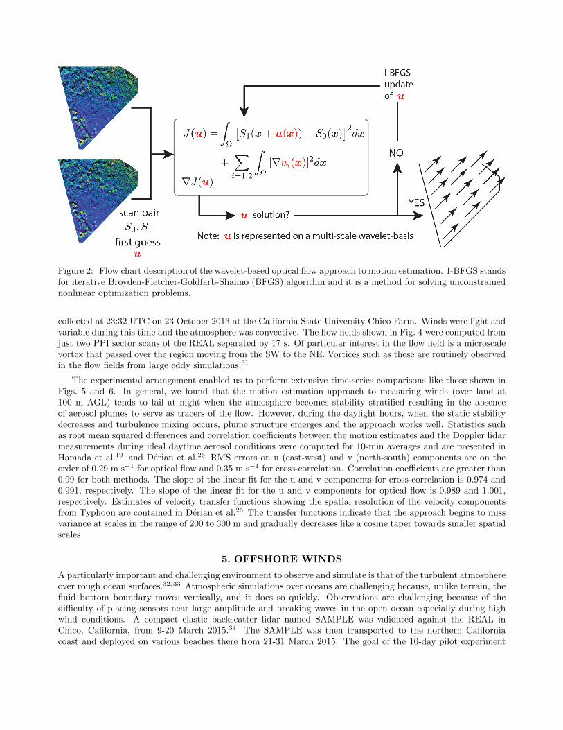
Figure 2: Flow chart description of the wavelet-based optical flow approach to motion estimation. I-BFGS standsfor iterative Broyden-Fletcher-Goldfarb-Shanno (BFGS) algorithm and it is a method for solving unconstrainednonlinear optimization problems.

collected at 23:32 UTC on 23 October 2013 at the California State University Chico Farm. Winds were light andvariable during this time and the atmosphere was convective. The flow fields shown in Fig. 4 were computed fromjust two PPI sector scans of the REAL separated by 17 s. Of particular interest in the flow field is a microscalevortex that passed over the region moving from the SW to the NE. Vortices such as these are routinely observedin the flow fields from large eddy simulations.31

The experimental arrangement enabled us to perform extensive time-series comparisons like those shown inFigs. 5 and 6. In general, we found that the motion estimation approach to measuring winds (over land at100 m AGL) tends to fail at night when the atmosphere becomes stability stratified resulting in the absenceof aerosol plumes to serve as tracers of the flow. However, during the daylight hours, when the static stabilitydecreases and turbulence mixing occurs, plume structure emerges and the approach works well. Statistics suchas root mean squared differences and correlation coefficients between the motion estimates and the Doppler lidarmeasurements during ideal daytime aerosol conditions were computed for 10-min averages and are presented inHamada et al.19 and Derian et al.26 RMS errors on u (east-west) and v (north-south) components are on theorder of 0.29 m s−1 for optical flow and 0.35 m s−1 for cross-correlation. Correlation coefficients are greater than0.99 for both methods. The slope of the linear fit for the u and v components for cross-correlation is 0.974 and0.991, respectively. The slope of the linear fit for the u and v components for optical flow is 0.989 and 1.001,respectively. Estimates of velocity transfer functions showing the spatial resolution of the velocity componentsfrom Typhoon are contained in Derian et al.26 The transfer functions indicate that the approach begins to missvariance at scales in the range of 200 to 300 m and gradually decreases like a cosine taper towards smaller spatialscales.

5. OFFSHORE WINDS

A particularly important and challenging environment to observe and simulate is that of the turbulent atmosphereover rough ocean surfaces.32,33 Atmospheric simulations over oceans are challenging because, unlike terrain, thefluid bottom boundary moves vertically, and it does so quickly. Observations are challenging because of thedifficulty of placing sensors near large amplitude and breaking waves in the open ocean especially during highwind conditions. A compact elastic backscatter lidar named SAMPLE was validated against the REAL inChico, California, from 9-20 March 2015.34 The SAMPLE was then transported to the northern Californiacoast and deployed on various beaches there from 21-31 March 2015. The goal of the 10-day pilot experiment

100 m

1523 m

REAL Lidar System Doppler Lidar

≈

≈

107 m

4 o

43 o

Figure 3: Diagram showing the vertical geometry of the 2013-14 field experiment in Chico, California. Distancesshown are not to scale.

Figure 4: Experimental results from Chico, California on 23 October 2013. Left panel: Vector flow field fromthe cross-correlation algorithm. Right panel: Vector flow field from the wavelet-based optical flow algorithm.The top panels are expansions of the area outlined by the white rectangle in the lower panels. The light bluedots on the light blue circle represent the sample volumes of the Doppler lidar at 100 m AGL. Vectors shown aresubsampled from the full vector fields for clarity. A microscale vortex can be observed near the middle of thescan area.

16:00 18:00 20:00 22:00 00:00 02:000 0

2 2

4 4

6 6

8 8

10 10Speed (

ms−

1)

16:00 18:00 20:00 22:00 00:00 02:000 0

90 90

180 180

270 270

360 360

Dir

ect

ion (◦)

Figure 5: Time-series from Gale (green) and the Doppler lidar (blue). Individual measurements are shown with+ symbols. Solid lines represent 10-minute running means.

16:00 18:00 20:00 22:00 00:00 02:000 0

2 2

4 4

6 6

8 8

10 10

Speed (

ms−

1)

16:00 18:00 20:00 22:00 00:00 02:000 0

90 90

180 180

270 270

360 360

Dir

ect

ion (◦)

Figure 6: Time-series from Typhoon (orange) and the Doppler lidar (blue). Individual measurements are shownwith + symbols. Solid lines represent 10-minute running means.

was to determine whether a compact micropulse lidar like the SAMPLE could be used to observe spray frombreaking waves and estimate the wind field over rough ocean surfaces. The Pacific Ocean along the northernCalifornia coast is notoriously rough but unfortunately the weather conditions were such that we only observedhigh amplitude sea states (2.4 – 3.6 m) on the last day of the experiment.

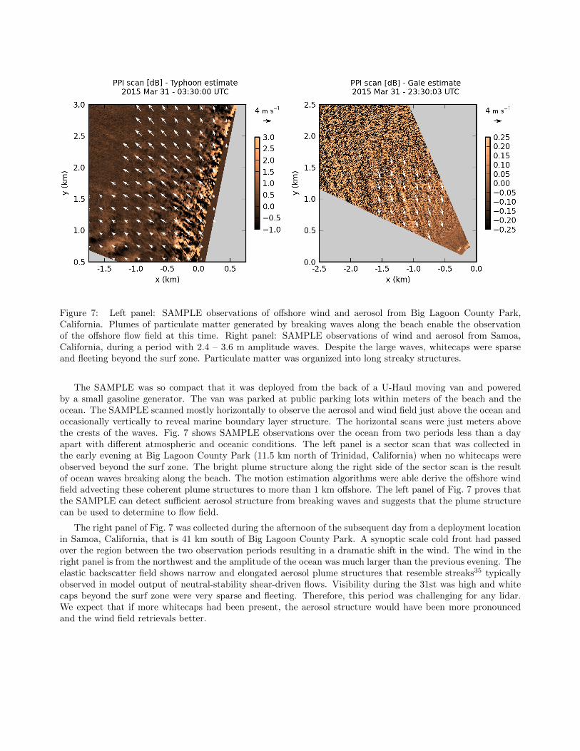
Figure 7: Left panel: SAMPLE observations of offshore wind and aerosol from Big Lagoon County Park,California. Plumes of particulate matter generated by breaking waves along the beach enable the observationof the offshore flow field at this time. Right panel: SAMPLE observations of wind and aerosol from Samoa,California, during a period with 2.4 – 3.6 m amplitude waves. Despite the large waves, whitecaps were sparseand fleeting beyond the surf zone. Particulate matter was organized into long streaky structures.

The SAMPLE was so compact that it was deployed from the back of a U-Haul moving van and poweredby a small gasoline generator. The van was parked at public parking lots within meters of the beach and theocean. The SAMPLE scanned mostly horizontally to observe the aerosol and wind field just above the ocean andoccasionally vertically to reveal marine boundary layer structure. The horizontal scans were just meters abovethe crests of the waves. Fig. 7 shows SAMPLE observations over the ocean from two periods less than a dayapart with different atmospheric and oceanic conditions. The left panel is a sector scan that was collected inthe early evening at Big Lagoon County Park (11.5 km north of Trinidad, California) when no whitecaps wereobserved beyond the surf zone. The bright plume structure along the right side of the sector scan is the resultof ocean waves breaking along the beach. The motion estimation algorithms were able derive the offshore windfield advecting these coherent plume structures to more than 1 km offshore. The left panel of Fig. 7 proves thatthe SAMPLE can detect sufficient aerosol structure from breaking waves and suggests that the plume structurecan be used to determine to flow field.

The right panel of Fig. 7 was collected during the afternoon of the subsequent day from a deployment locationin Samoa, California, that is 41 km south of Big Lagoon County Park. A synoptic scale cold front had passedover the region between the two observation periods resulting in a dramatic shift in the wind. The wind in theright panel is from the northwest and the amplitude of the ocean was much larger than the previous evening. Theelastic backscatter field shows narrow and elongated aerosol plume structures that resemble streaks35 typicallyobserved in model output of neutral-stability shear-driven flows. Visibility during the 31st was high and whitecaps beyond the surf zone were very sparse and fleeting. Therefore, this period was challenging for any lidar.We expect that if more whitecaps had been present, the aerosol structure would have been more pronouncedand the wind field retrievals better.

6. SUMMARY

Five general points are worth pointing out. First, a new wavelet-based optical flow motion estimation algorithm(named Typhoon) has been developed and it appears to be able to resolve smaller scale velocity features thancross-correlation. Second, by comparing the velocity estimates with those from a Doppler lidar, an acceptedstandard for wind measurement, we have begun to quantify accuracy and precision. In addition (third), wehave estimated the spatial resolution of the Typhoon velocity fields by computing spatial power spectra andcomparing those spectra with estimates based on Kolmogorov’s inertial subrange hypothesis. However, manyfactors influence the accuracy, precision and resolution of the retrieved vector fields and much more work remainsto be done on this topic. For example, the mechanism by which turbulence is generated (shear or buoyancy)have a profound effect on the turbulence structure which in turn effects plume structure and retrieval of the flowfields. Furthermore, it may be possible to increase the spatial resolution of the flow fields by adjusting the scanrate and azimuthal range of the lidar scans. Fourth, a new and compact elastic backscatter lidar has becomeavailable that can be used economically to probe the aerosol field just above wave crests. Further improvementsin lidar performance are likely. Finally, a pilot experiment confirmed the hypothesis that the particulate mattergenerated by breaking ocean waves is more than adequate for such a lidar to detect. In the future, we wishto deploy a SAMPLE with a suite of other instruments on the coast and observe rough oceans with abundantwhitecaps. We will use these observations to validate simulations of lower atmosphere turbulence structure andadvance theories on air-sea interaction.

ACKNOWLEDGMENTS

This work was supported by the National Science Foundation’s Physical and Dynamic Meteorology Programunder awards AGS 0924407 and 1228464. Deployment of the SAMPLE in Chico CA in March 2015 was supportedby HDTRA2-15-C-0003. Deployment of the SAMPLE in Eureka CA in March 2015 was supported by NSF AGS1536624.

REFERENCES

[1] Gurka, R. and Kit, E., “Optical methods and unconventional experimental setups in turbulence research,”in [Handbook of Environmental Fluid Dynamics, Vol. 2 ], Fernando, H. J. S., ed., CRC Press/Taylor andFrancis Group, LLC. (2013).

[2] Velden, C., Daniels, J., Stettner, D., Santek, D., Key, J., Dunion, J., Holmlund, K., Dengel, G., Bresky, W.,and Menzel, P., “Recent innovations in deriving tropospheric winds from meteorological satellites,” Bulletinof the American Meteorological Society 86(2), 205–223 (2005).

[3] Murray, J. C., Erwin, H. R., and Wermter, S., “Robotic sound-source localisation architecture using cross-correlation and recurrent neural networks,” Neural Networks 22(2), 173–189 (2009).

[4] Emery, W. J., Baldwin, D., and Matthews, D., “Maximum cross correlation automatic satellite imagenavigation and attitude corrections for open-ocean image navigation,” IEEE T. Geosci. Remote Sens. 41(1),33–42 (2003).

[5] Avants, B. B., Epstein, C. L., Grossman, M., and Gee, J. C., “Symmetric diffeomorphic image registrationwith cross-correlation: evaluating automated labeling of elderly and neurodegenerative brain,” Med. ImageAnal. 12(1), 26–41 (2008).

[6] Schubert, A., Faes, A., Kaab, A., and Meier, E., “Glacier surface velocity estimation using repeat TerraSAR-X images: Wavelet vs. correlation-based image matching,” Int. Soc. Photogramme. 82, 49–62 (2013).

[7] Adrian, R. J. and Westerweel, J., [Particle Image Velocimetry ], Cambridge University Press (2011).

[8] Cheng, W., Murai, Y., Sasaki, T., and Yamamoto, F., “Bubble velocity measurement with a recursive crosscorrelation PIV technique,” Flow Meas. Instrum. 16(1), 35–46 (2005).

[9] Antoine, E., Buchanan, C., Fezzaa, K., Lee, W.-K., Rylander, M. N., and Vlachos, P., “Flow measurementsin a blood-perfused collagen vessel using x-ray micro-particle image velocimetry,” PLOS ONE 8(11), e81198(2013).

[10] Leese, J. A., Novak, C. S., and Clark, B. B., “An automated technique for obtaining cloud motion fromgeosynchronous satellite data using cross correlation,” J. Appl. Meteorol. 10(1), 118–132 (1971).

[11] Garcıa-Pereda, J. and Borde, R., “The impact of the tracer size and the temporal gap between images inthe extraction of atmospheric motion vectors,” J. Atmos. Ocean. Technol. 31(8), 1761 – 1770 (2014).

[12] Rinehart, R. E. and Garvey, E. T., “Three-dimensional storm motion detection by conventional weatherradar,” Nature 273, 287–289 (1978).

[13] Eloranta, E. W., King, J. M., and Weinman, J. A., “The determination of wind speeds in the boundarylayer by monostatic lidar,” J. Appl. Meteor. 14, 1485–1489 (1975).

[14] Shimizu, H., Sasano, Y., Yasuoka, Y., Ueda, H., Takeuchi, N., and Okuda, M., “The remote measurementof wind direction and velocity by a laser radar using the spatial correlation technique,” Oyobutsuri 50,616–620 (1981).

[15] Kolev, I., Parvanov, O., and Kaprielov, B., “Lidar determination of winds by aerosol inhomogeneities:motion velocity in the planetary boundary layer,” Appl. Optics 27, 2524–2531 (1988).

[16] Mayor, S. D. and Eloranta, E. W., “Two-dimensional vector wind fields from volume imaging lidar data,”J. Appl. Meteor. 40, 1331–1346 (2001).

[17] Mayor, S. D., Lowe, J. P., and Mauzey, C. F., “Two-component horizontal aerosol motion vectors in theatmospheric surface layer from a cross-correlation algorithm applied to scanning elastic backscatter lidardata,” J. Atmos. Ocean. Technol. 29, 1585–1602 (2012).

[18] Hamada, M., Evaluation of the performance of a cross-correlation algorithm for wind velocity estimationusing synthetic backscatter lidar images and velocity fields, diploma thesis, California State University, Chico,400 West First Street, Chico CA 95929 (Aug 2014).

[19] Hamada, M., Derian, P., Mauzey, C. F., and Mayor, S. D., “Optimization of the cross-correlation algorithmfor two-component wind field estimation from single aerosol lidar data and comparison with Doppler lidar,”Submited to J. Atmos. Ocean. Technol. (2015).

[20] Horn, B. K. P. and Schunck, B. G., “Determining optical flow,” Artificial Intelligence 17, 185–203 (1981).

[21] Heitz, D., Memin, E., and Schnorr, C., “Variational fluid flow measurements from image sequences: synopsisand perspectives,” Experiments in Fluids 48(3), 369–393 (2010).

[22] Corpetti, T., Heitz, D., Arroyo, G., Memin, E., and Santa-Cruz, A., “Fluid experimental flow estimationbased on an optical-flow scheme,” Exp. Fluids 40(1), 80–97 (2006).

[23] Derian, P., Heas, P., Memin, E., and Mayor, S. D., “Dense motion estimation from eye-safe aerosol lidardata,” in [Proceedings of the 25th International Laser Radar Conference ], 1, 377–380 (2010).

[24] Derian, P., Wavelets and Fluid Motion Estimation, PhD thesis, MATISSE, Universite Rennes 1 (2012).[Available online at http://tel.archives-ouvertes.fr/tel-00761919/PDF/theseDERIAN v3 BU .pdf.].

[25] Derian, P., Heas, P., Herzet, C., and Memin, E., “Wavelets and optical flow motion estimation,” NumericalMathematics Theory, Methods, and Applications (2012).

[26] Derian, P., Mauzey, C. F., and Mayor, S. D., “Wavelet-based optical flow for two-component wind fieldestimation from single aerosol lidar data,” J. Atmos. Ocean. Technol. (In Press) (2015).

[27] Mauzey, C. F., Lowe, J. P., and Mayor, S. D., “Real-time wind velocity estimation from aerosol lidar datausing graphics hardware,” GPU Technology Conference, San Jose, CA (May 2012). Poster presentationAV10.

[28] Mayor, S. D. and Spuler, S. M., “Raman-shifted Eye-safe Aerosol Lidar,” Appl. Optics 43, 3915–3924 (2004).

[29] Spuler, S. M. and Mayor, S. D., “Scanning eye-safe elastic backscatter lidar at 1.54 microns,” J. Atmos.Ocean. Technol. 22, 696–703 (2005).

[30] Mayor, S. D., Spuler, S. M., Morley, B. M., and Loew, E., “Polarization lidar at 1.54-microns and observa-tions of plumes from aerosol generators,” Opt. Eng. 46, DOI: 10.1117/12.781902 (2007).

[31] Kanak, K. M., “Numerical simulation of dust devil-scale vortices,” Quart. J. R. Met. Soc. 131(607), 1271–1292 (2005).

[32] Mayor, S. D., Derian, P., Mauzey, C. F., and Hamada, M., “Observations of two-component wind fields fromaerosol lidar and motion estimation algorithms including first results over rough sea states,” InternationalConference on Model Integration across Disparate Scales in Complex Turbulent Flow Simulation (June2015). Paper 28.

[33] Sullivan, P. P., McWillians, J. C., and Patton, E. G., “Large-eddy simulation of martine atmosphericboundary layers above a spectrum of moving waves,” J. Atmos. Sci. 71, 4001–4027 (2014).

[34] Mayor, S. D., Derian, P., Mauzey, C. F., Spuler, S. M., Ponsardin, P., Pruitt, J., Ramsey, D., and Higdon,N. S., “Comparison of aerosol backscatter and wind field estimates from REAL and SAMPLE,” SPIE(August 2015). Paper 9612-16.

[35] Drobinski, P. and Foster, R., “On the origin of near-surface streaks in the neutrally-stratified planetaryboundary layer,” Bound. Layer Meteor. 108(2), 247–256 (2003).