Technical Report Pattern Recognition and Image Processing GroupInstitute of Computer Aided AutomationVienna University of TechnologyFavoritenstr. 9/183-2A-1040 Vienna AUSTRIAPhone: +43 (1) 58801-18351Fax: +43 (1) 58801-18392E-mail: {me}@mail.comURL: http://www.prip.tuwien.ac.at/

PRIP-TR-118 October 16, 2008

Spherical WaveletsA new tool for 3D shape representation

Schwartz Ernst

Abstract

Wavelets are a common tool for the analysis of signals in one or two dimensions. Extendingthose findings to be used in a three-dimensional setting has proven more difficult. Thisreport is concerned with a recent promising approach to wavelet analysis in 3 dimensions ongenus-0 objects, the so-called spherical wavelets. Using examples from the field of medicalimaging, the concepts underlying their construction are introduced and their usefullnessfor a variety of applications is demonstrated. Further, an overview of publicly availabletoolboxes is given and an evaluation comparing the capabilities of spherical wavelets todifferent shape modelling approaches is performed.

Contents

1 Introduction 2

2 Preliminaries 42.1 The Fourier transform . . . . . . . . . . . . . . . . . . . . . . 42.2 Introducing Wavelets . . . . . . . . . . . . . . . . . . . . . . . 52.3 2nd generation wavelets . . . . . . . . . . . . . . . . . . . . . 8

2.3.1 Polyphase representation . . . . . . . . . . . . . . . . . 92.3.2 Factoring filters using the lifting scheme . . . . . . . . 112.3.3 Construction of wavelets using the lifting scheme . . . 12

3 Spherical Wavelet Shape Representation 143.1 State-of-the art representations of 3D objects . . . . . . . . . . 143.2 Spherical representation of 3D objects . . . . . . . . . . . . . . 163.3 The construction of spherical wavelets . . . . . . . . . . . . . 193.4 Using spherical wavelets for shape representation . . . . . . . 20

3.4.1 Filtering . . . . . . . . . . . . . . . . . . . . . . . . . . 203.4.2 Band-wise grouping . . . . . . . . . . . . . . . . . . . . 213.4.3 Dimensionality reduction . . . . . . . . . . . . . . . . . 21

3.5 Implementation . . . . . . . . . . . . . . . . . . . . . . . . . . 233.5.1 Matlab Wavelet Toolbox . . . . . . . . . . . . . . . . . 233.5.2 YAWTB; yet another wavelet toolbox . . . . . . . . . . 233.5.3 Gabriel Peyres toolboxes . . . . . . . . . . . . . . . . . 233.5.4 Spherical wavelet ITK filter . . . . . . . . . . . . . . . 24

3.6 Putting it all together . . . . . . . . . . . . . . . . . . . . . . 24

4 Applications & Experiments 264.1 Applications . . . . . . . . . . . . . . . . . . . . . . . . . . . . 26

4.1.1 Signal description . . . . . . . . . . . . . . . . . . . . . 264.1.2 3D modelling . . . . . . . . . . . . . . . . . . . . . . . 264.1.3 Segmentation . . . . . . . . . . . . . . . . . . . . . . . 26

4.2 Experiments . . . . . . . . . . . . . . . . . . . . . . . . . . . . 284.2.1 Compression . . . . . . . . . . . . . . . . . . . . . . . . 284.2.2 Band-wise grouping . . . . . . . . . . . . . . . . . . . . 304.2.3 Shape description . . . . . . . . . . . . . . . . . . . . . 31

5 Conclusion 33

1

1 Introduction

Modern imaging techniques for medical applications have reached a level ofsophistication during the last 10 years that allows for a sub-millimeter pre-cision on MRIs or CTs. While this is of great help for professionals andscientists in the field of medicine, the precision achieved is maybe of evengreater help for automatic analysis using image processing and machine vi-sion.Today, most analysing of x-rays or other images is still done by evaluating2d slices separately. Because of the 3d nature of the anatomical structures,this can be very ineffective, nevertheless professionals are still reluctant touse the 3d data directly, because of the high complexity of the stuctures, andthe lack of intuitive and efficient interfaces.One important research area to improve the acceptance of 3d imaging inthe medical community is the (semi-)automatic segmentation of the data toeliminate the possibility of one structure hiding others or the like.

In this report, we will investigate a novel approach to representing 3d datathat has provided promising results for signal analysis, shape description andconsequently segmentation purposes; the spherical wavelet representation.To gain a better understanding of what exactly such a representation is, howit is computed and how it can be used in a medical imaging context, we willstart not with a 3d signal but a simple 1d one, such as a time series. Af-ter presenting the idea of a harmonic expansion using the standard Fouriertransform in section 2.1, in the following section 2.2 we will look more indepth at the oldest, the so called ”Haar” wavelet, before investigating waysof constructing more sophisticated representations in section 2.3. Once thereader is familiar with the basics of wavelet theory, we will look at how todescribe 3d objects in a way that enables us to deal with them in a signalprocessing framework (sections 3.1 to 3.4) and present, in section 3.5, differ-ent available software packages for (spherical) wavelet analysis.

In section 4, we will give a quick overview over some applications of sphericalwavelets today, which range from astrophysics to medical applications anddo a comparitive study of the spherical wavelet approach and other com-monly used compressing signal representations. In the experimental results(section 4.2), we will demonstrate in a step-by-step manner how to computethe so-called spherical wavelets from these representations.

2

3

2 Preliminaries

2.1 The Fourier transform

In signal analysis, one often reaches the limits of gainable knowledge aboutthe contained information in a specific representation of the signal.By applying a transform to the signal, it is often possible to find propertiesof the signal that where hidden before.For instance, the complexity of language stems from the fact that humanhearing works by processing different frequencies of the sounds that reachthe inner ear and combining that information into a representation that thehuman brain is able to interpret. This type of analysis can either be achievedby separating different frequencies of the signal using a so called filter bankor by the Fourier transform, one of the earliest types of transforms that wasshown to be able to fully describe the information contained in the signal,e.g. to be fully invertible.The Fourier decomposes a function into a series of coefficients associated totrigonometric functions, that is a series of sines and cosines with a certainamplitude and phase.

x(t) =

∫ ∞−∞

X(f)ei2πftdt (1)

When someone mentions a sound having a high frequency, what this ac-tually means are larger Fourier coefficients in the upper part of the so-calledspectrum, the amplitude of the totallity of the signals components.The Fourier transform is by no means limited to the analysis of one-dimensionalsignals. There exist analysis methods based on the Fourier transform for 2dand even 3d signals, then more appropriately called images or shapes.

One serious drawback of the Fourier transform though is its inability tolocalize components in the signal. Because it decomposes the signal into anintegral of infinite functions (sines / cosines), the analysis of a signal thatchanges with time (or space, for images, eg. is not a pattern) can becomeuseless as there is, in the Fourier domain, no way of telling when in time acomponent of a certain frequency starts and stops. To counter this effect, theonly way to gain useful temporal information from the Fourier (or frequency)representation of a signal was to first decompose it into small parts and an-

4

alyze those separately. This is called the windowed Fourier transform [8]because one uses a windowing function (in the simplest case a box functionof a certain width) to cut the signal. By using more complexly constructedwindows, one can achieve a better separation and less distortion. In fact, thetransform this report is mainly concerned with, the wavelet transform, canbe seen as a sort of formalization of the windowed Fourier transform, as wewill see next.

2.2 Introducing Wavelets

The first wavelet transform wasnt actually called such, the term being coinedby Stephane Mallat [9] . Long before that, in 1909, Alfred Haar proposedwhat became known as the Haar wavelet, a very simple form of a waveletthat works by dyadic subsampling of the signal and using the differencesbetween samples.

To perform a Haar decomposition of a signal of length 2n (also called Haarwavelet transform), one first splits the signal into even and odd samples.The two resulting signals now have the same length, n.

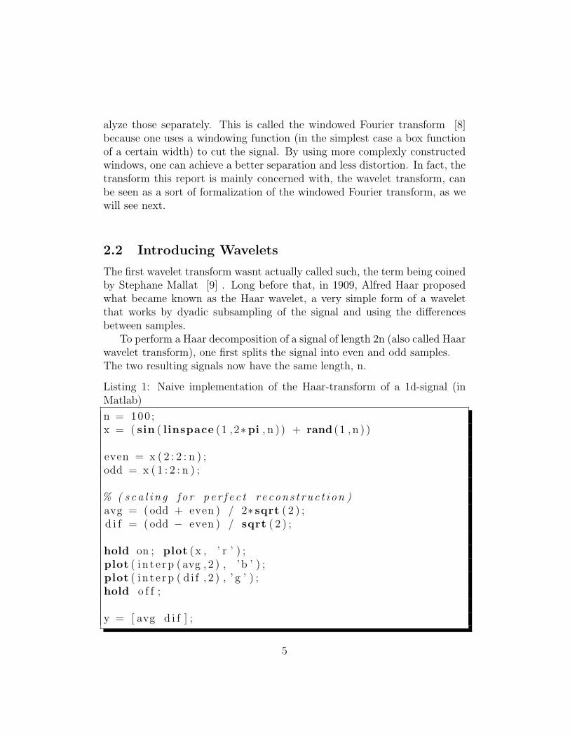
Listing 1: Naive implementation of the Haar-transform of a 1d-signal (inMatlab)

n = 100 ;x = ( sin ( linspace (1 ,2∗pi , n ) ) + rand (1 , n ) )

even = x ( 2 : 2 : n ) ;odd = x ( 1 : 2 : n ) ;

% ( s c a l i n g f o r p e r f e c t r e c o n s t r u c t i o n )avg = ( odd + even ) / 2∗ sqrt ( 2 ) ;d i f = ( odd − even ) / sqrt ( 2 ) ;

hold on ; plot (x , ’ r ’ ) ;plot ( i n t e r p ( avg , 2 ) , ’b ’ ) ;plot ( i n t e r p ( d i f , 2 ) , ’ g ’ ) ;hold o f f ;

y = [ avg d i f ] ;

5

Figure 1: toy example for a Haar decomposition: original signal in red,(upsampled) averages in blue, details in green

The next step in the transform is to add the two signals together andnormalize on one hand (averages), and subtract and normalize on the otherhand (detail).Note that the resulting average and detail coefficients retain the completeinformation about the signal.

A complete Haar-transform of a signal consists in repeating the abovesteps for the averages until only a single scalar describing the averages (ameasure of the DC component of the signal) and the detail coefficients ofeach step are left.It should be noted here that the Haar transform (and other wavelet trans-forms too) are not reducing the size of the data directly. In fact, the sizeof the wavelet decomposition (e.g. the concatenation of the average and thedetail coefficients) is of exactly the same length as that of the original signal.What makes wavelet decomposition interesting for data compression (it hasfor example replaced DCT-based coding in the jpeg2000 image standard [20])

6

is the fact that many of the detail coefficients, especially at higher decom-position levels, turn out to be rather small in magnitude and can thus beneglected (zeroed out), by which a quite impressive data reduction rate canbe achieved without distorting the original signal too much.

Before plunging into the mathematical description of the wavelet trans-form, lets take a quick look at some common names and notations used inthe literature.As we have seen, the wavelet transform decomposes a signal into averagesand detail coefficients. The name average might be well fitted for the sim-ple Haar-transform, but for more elaborate wavelets, it can be misleading.The functions to compute the averages are commonly called scaling functionswhilst the one for the details are being called wavelet functions.With this in mind, lets take a look at the mathematical description of thewavelet transform and some of the properties that make it interesting forsignal analysis.

The general formula of a wavelet transform is

ψa,b(t) =1√aψ(t− ba

) (2)

xa(t) =

∫ ∫x(t)ψa,b(t)dt (3)

Comparing it to (1), one can see the similarities. A wavelet transformis comparable to a windowed Fourier transform with scaled and shifted win-dows, thus capturing low and high frequency components of the signal atspecific locations in time or space.

The Haar-wavelet being a very simplistic transform it has some unde-sirable properties such as aliasing effects due to its binary nature. Thus,extensions have been proposed for constructing more sophisticated wavelets.For a detailed description of these as well as corresponding derivations theinterrested reader is reffered to the classical text in the field by Daubechies[1].These constructions are far from trivial. To ensure such properties as fullreconstructability and orthogonality of the composing functions, one needsto perform a thorough mathematical analysis of the wavelet in question.

7

A somewhat simpler and more elegant method for constructing new (andcommon) wavelets and enforcing some desired properties onto them is theso called lifting scheme proposed by Sweldens in [2], [19] which will bedescribed next.

2.3 2nd generation wavelets

The description of the lifting scheme will start with a slight change of nota-tion. As we have seen, each step in the wavelet transform splits the signalinto two parts, which can be interpreted as a low frequency one and a highfrequency one that can be recombined to reconstruct the original signal.

As the transform can be described in terms of frequency information ex-tracted from the signal, and remembering the filtering approach to signalanalysis from chapter 2.1, it is but logical to try and define it as (a cascadeof) filtering operations.

Listing 2: Filter implementation of Haar transform

n = 100 ;x = ( sin ( linspace (1 ,2∗pi , n ) ) + rand (1 , n ) )

h = [ 1 1 ] / 2 ; % averag ing f i l t e r sums to 1g = [−1 1 ] ; % d i f f e r e n c i n g f i l t e r to 0

avg = f i l t e r (h , 1 , x ) / sqrt ( 2 ) ;avg = avg ( 2 : 2 : end ) ’ ;

d i f = f i l t e r ([−1 1 ] , 1 , x ) / sqrt ( 2 ) ;d i f = d i f ( 2 : 2 : end ) ’ ;

From now on, we will denote the filters used for that decomposition as hand g and those for reconstruction as h and g respectively. A transform canthus by represented like in figure 2

where the filters have to fullfil the conditions (4) and (5:

8

Figure 2: wavelet decomposition; filtering interpretation

h(z)h(z−1) + g(z)g(z−1) = 2 (4)

h(z)h(z−1) + g(z)g(−z−1) = 0 (5)

2.3.1 Polyphase representation

Looking at Figure 2, one can immediately spot an inefficiency in the im-plementation. As half the samples are thrown away each step, it would bemuch more efficient to apply the filters only to those samples that are ac-tually needed and disregard the others. This is achieved by the so-calledpolyphase representation.

Figure 3: polyphase decomposition

9

That representation can be put into matrix form, which leaves us with

P (z) =

(he(z) ho(z)ge(z) go(z)

)(6)

describing the decomposition part of the wavelet transform. We can pro-ceed analogously with the reconstruction part, which gets us

P (z) =

(he(z) ge(z)ho(z) go(z)

)(7)

and thus

Figure 4: polyphase wavelet decomposition

Listing 3: Polyphase implementation of Haar transform

odd = x (end−1:−2:1);even = x (end : −2 :2 ) ;

s = conv (h ( 1 : 2 : end ) , odd ) + conv (h ( 2 : 2 : end ) , even )d = conv ( g ( 1 : 2 : end ) , odd ) + conv ( g ( 2 : 2 : end ) , even )

s = [ s (1)+ s (end) s (end−1 :−1 :2) ] ;d = [ d(1)+d(end) d(end−1 :−1 :2) ] ;

As it turns out, the polyphase matrix is a matrix of Laurent polynomialsof the form h(z) =

∑qk=p hkz

−k, which have the property that sums, differ-ences, products and even divisions (with rest) of Laurent polynomials arethemselves Laurent polynomials.

10

Because such Laurent polynomials can be interpreted as discrete filters, thisproperty can be exploited in the so-called Lifting scheme.

2.3.2 Factoring filters using the lifting scheme

It is possible to factor the filters involved in the wavelet decomposition andreconstruction in simpler ones, thus reducing costly convolutions to shorterones or even simple multiply- and add-operations by solving small systems ofequations. Depending on the original complexity of the scaling and waveletfilters, this results in a speed increase of up to 100% for certain types ofwavelets.For the reconstruction part, this corresponds to solving for the primary liftingcoefficient and rests in

P (z) =

(he(z) ho

new(z)

ge(z) gonew(z)

)∗(

1 s(z)0 1

)(8)

or for the dual lifting coefficients and rest in

P (z) =

(he

new(z) ho(z)

genew(z) go(z)

)∗(

1 0t(z) 1

)(9)

The construction is analogous for the analysis part.

The following applies the lifting scheme decomposition to reformulate theHaar transform. Note that, because the filters involved are allready of length2, this does not result in a speed increase. It is nonetheless a usefull exampleto understand the workings of the lifting scheme.In a polyphase formulation, the now familiar Haar transform coresponds to

P (z) =

(1/2 1/2−1 1

)The lifting scheme can be applied to this, leaving us to solve

P (z) =

(he

new(z) 1/2

genew(z) 1

)∗(

1 0t(z) 1

)11

and thus henew

(z) +1

2∗ t(z) =

1

2genew(z) + t(z) = −1

Setting henew

(z) = 1 gives

P (z) =

(1 1/20 1

)∗(

1 0−1 1

)

which results in the follwing implementation

Listing 4: Lifted haar transform

odd = x ( 1 : 2 : end ) ;even = x ( 2 : 2 : end ) ;

% second matrixd = odd − even ;

% f i r s t matrixs = .5∗d + even

2.3.3 Construction of wavelets using the lifting scheme

On the other hand, the factorability of Laurent polynomials allows to gener-ate more sophisticated wavelets (lift the original wavelet) from really basicones by multiplying the decomposition filter by a carefully selected Laurentpolynomial

gnew(z) = g(z) + h(z)s(z2) (10)

12

P new(z) =

(he(z) he(z)s(z) + ge(z)ho(z) ho(z)s(z) + go(z)

)= P (z)

(1 s(z)0 1

)(11)

and analogously in the reconstruction part

hnew(z) = h(z) + g(z)s(z2) (12)

P new(z) =

(he(z) + ge(z)s(z) ho(z) + go(z)s(z)

ge(z) go(z)

)=

(1 s(z)0 1

)P (z)

(13)

Figure 5: polyphase lifted wavelet decomposition

See figure 5 for a schematic representation of the primal lifting decompo-sition and reconstruction.

On the other hand, it is also possible to multiply the reconstruction filterfirst and find the appropriate Laurent polynomial to use in the decomposi-tion part afterwards. This procedure is then called dual lifting (opposed toprimal lifting in the first case).

Using the lifing scheme, basically all that is needed to perform a waveletanalysis on a signal are concise split and merge operators and some notionof neighbourhood of samples fo the signal.

13

That way, the lifting scheme turns out to be a very powerful method of adapt-ing the wavelet bases to the conditions encountered in the signal, and also toother realms than the one-dimensional case by defining split and merge op-erations (cf. the notes on multi-resolution later in this report) and carefullychoosing the lifting steps.Having now gained a firm understanding of how to decompose a signal usingwavelets and how to implement this process in a series of lifting steps, wecan now move to the core of this report, the spherical wavelets.After quickly reviewing current shape representation techniques, we will de-scribe in detail how shapes can be represented as spherical signals and howthese can in turn be decomposed by a wavelet analysis. These explanationswill be followed by an instructive example of the presented methods appliedto real-life data.

3 Spherical Wavelet Shape Representation

3.1 State-of-the art representations of 3D objects

Our work is concerned with the analysis of 3D objects and we will nowgive a quick overview over current methods of describing 3D objects in ausefull and efficient manner. We will begin with fundamental methods andcontinue with describing current, more elaborate approaches before arrivingat the representation that is essential for building (spherical) wavelets in a3D setting, the so-called multi-resolution framework.

Piecewise linear surface representation Maybe the most fundamentalmethod for 3D-modelling, along with voxel methods, is what is commonlyknown as piecewise linear surface representation. Here, objects are approxi-mated by a collection of surface polygons that generally are all of the sametype, eg. triangles or squares. The information on the structure is containedin a list of all points, the vertex list and a list of the connectivities betweenthese, the face list or surface mesh.If one is looking for a lower-dimensional analogy to this setting, one couldcompare the surface polygon approach to a 2D-vector-image, while the voxelrepresentation would correspond to the pixel-image.While this representation is amongst the oldest in computer graphics, it isalso still the most commonly used because of its nice mathematical proper-

14

ties and simple representation. All of the methods we are going to describenext are using it as their foundation.

Spline-based representation Splines are a well-known method for curvefitting using piecewise polynomial curves. Their use has mainly been mo-tivated by their easy construction and manipulation as well as their smallstorage requirements even for ”complicated” shapes. As such, it is possibleto represent a shape by a collection of control points, called knots for whichparameters are defined, the combination of which describing the shape ofthe curve. The points between two knots are then interpolated using thoseparameters, which explains the small storage requirements.Because of their small number of control points, spline-based models havefound applications in tracking problems, as for instance in [14] where theyhave been combined with multi-resolution methods for real-time performance.

Planar parametrizations Representing 3D-objects in 2 dimensions is anage old problem originating from map-making. Representing an object insuch a way has numerous advantages, from texture mapping to the possibil-ity of regular remeshing in the plane. Allthough, because of an - arguably -smaller distortion, the algorithm described in this paper uses not a mappingonto the plane but onto the unit sphere, the classical and recent develope-ments in planar mapping still provide usefull insights into the problem ofdescribing 3-dimensional structures. Various good overviews of the differenttechinques and mappings exist, for instance in [3].

Geometry images In a 3D-mesh, every point, or vertex, is fully describedby its coordinates in 3D-space, x, y and z. In 2D-imaging, color informationis also stored in a 3D-representation, namely the values for the red, greenand blue components. This analogy led Sweldens et al. [7] to build a cor-respondence between those two representations which they termed geometryimage. Here, every pixel in the image actually is a vertex of a 3D-model, andthe color information represents the spacial information of that vertex.To build a geometry image from a 3D object, one needs to sample this spacialinformation for a number of points on the mesh. This sampling needs to beregular so as not to produce under- or oversampled regions of the geometry.For this, different sampling schemes that are also very usefull for sphericalresampling have been proposed. We will describe those in more detail in a

15

later section of this report.

Laplacian framework One reason why mesh-representations of 3D-objectsare so widely used is the availability of well-studied mathematical models insuch a framework. If a model is described by a mesh, methods from graph-theory can be applied to it. In recent years, spectral graph theory has gaineda lot of interest in the computer science community for its ability to representthe information contained in a graph in usefull ways.The Laplacian framework is the result of this. The Laplacian matrix of amesh is a variant to the well-known connectivity matrix, with some additionalinformation on the structure of the underlying mesh. On this matrix, one canperform an eigenanalysis to extract the main components of the mesh. Thisapproach can then be used for different processing operations on 3D-objects,from approximation to editing and watermarking. A detailed discussion isbehond the scope of this report, and interested readers are referred to [13]for more information.

Multi-resolution analysis As seen before, wavelet analysis is based oncomputing differences between neighbouring samples of a signal. To be ableto perform this operation on a 3D-mesh, the representation of the meshsomehow needs to contain this neighbourhood information. Multi-resolutionanalysis provides extactly this - it represents an object as a series of mesheson different levels of detail. Going from coarse to fine in this frameworkmeans inserting new vertices between existing ones in a well-defined manner.For a detailed description of methods for multi-resolution analysis, see [5]or [23].

3.2 Spherical representation of 3D objects

Until now, we only analyized signals in a one or two-dimensional setting.Since our ultimate goal is to develop methods to work on three-dimensionalobjects, one needs to settle for a representation of these objects that allowsfor the required mathematical operations to be performed without any in-consistencies or undefined behaviour.To achieve this, we will consider a spherical signal representation, meaningthat we will be concerned with signals sampled on a sphere. There are dif-ferent ways to sample from a sphere, (cf fig 6), but because of its regularity,

16

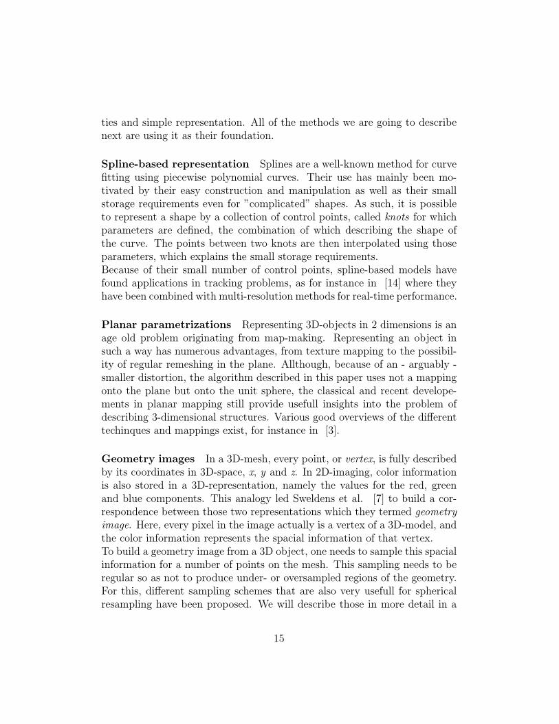
which eliminates over- and undersampled regions, an icosahedron-based sub-division is most commonly used. It is built by starting with an icosahedronand recursively subdividing each of its faces recursively into 4 new triangles(cf. figure 6).

Figure 6: regular and icosehedron-based sampling on the sphere

Mesh representations of three-dimensional objects can be mapped to thesphere if they are of genus-0, e.g. topologically equivalent to a sphere anddo not contain holes.The way this is done is to first find a minimally distorted mapping of thefaces of the mesh onto the sphere while retaining the original coordinates foreach vertex.Finding this mapping is in itself far from trivial. Early approaches werebased on efforts to extend the method of barycentric coordinates for planarparametrizations to the 3D case, but were unable to generate a bijectivemapping. Later, Sweldens and proposed what he called a progressive meshconstruction, which consists of removing vertices one by one from the meshwhilst storing the connectivity information of each removed vertex until onlyan icosahedron (or another platonic solid which can be inscribed in a sphere)remains and then adding the vertices back into the mesh, positioning themon the sphere and moving them to minimize distortions and eliminate fold-overs.

17

While that construction achieves satisfying results, it is quite slow and theoptimization procedure is difficult to influence.Lately, approaches based on spectral graph and Laplacian methods haveshown usefull for the task. However, they involve solving large systems ofnon-linear equations and can thus be computationally expensive.A good overview over all these methods can be gained from [6] or [4].

Figure 7: Icosahedron based subdivision of the Stanford bunny

Once the points are mapped, the x, y and z coordinates are consideredto be functions on the sphere (e.g. to fully describe a 3d object, there areactually 3 spheres). As these functions are unevenly sampled, one now needsto resample them on a regular grid on the sphere as seen before.

In clinical studies a specific organ or anatomical structure is observed overa range of patients, or during a period of time for a single patient. The topol-ogy of the observed structure can be assumed consistent over all examples. Awidely used approach to study the variation of shapes is to first compute themean shape from the remeshed shape population. Subsequently a specificexample can be encoded by describing the vertex-wise deviation from themean shape.To recapitulate, we have started out with a mesh consisting of vertices ina three-dimensional euclidean space, which we mapped to a sphere by adistortion-minimizing method. Now, this representation is resampled us-ing a regular, subdivisible mesh defined on the sphere, resulting in a multi-resolution representation of the original shape.

18

3.3 The construction of spherical wavelets

After defining how to map a given mesh onto a sphere and how to samplea signal from it, we can begin describing the spherical wavelet analysis perse. This analysis will allow us to efficiently represent the deviation from themean shape as spherical wavelet components.A wavelet decomposition of a signal always consists of a subsampling anda differencing step. The same is now done on the sphere. Subsampling isachieved by retaining only a broader mesh representation of the sphere, whichmust be a real subset of the original mesh. That way, we perform a so-calledmulti-resolution analysis, and we are left with a representation of a signal onthe sphere composed of elements with decreasing resolution. For a detailedderivation, see [16] and [15].As we have seen, this by itself is not very helpful because the informationbetween two sampling levels is simply lost (this simple subsampling is com-monly called the lazy transform).To recover that information, one could simply use a Haar-like operator, whichretains the differences between two stages. That approach, however, intro-duces some undesired aliasing effects. Here, the lifting scheme is used togenerate more complex, better-adapted filters on the sphere, called stencils(cf. figure 8), that can be interpreted as analogues to the filter taps of thescaling- and wavelet filters in a lower-dimensional setting. Such stencils warryfrom simple neighbourhoods to wider ones, the later resulting in a smootherdecomposition.

Figure 8: linear, quadratic and butterfly stencils for center (red) point

Using these stencils, for each point a neighbourhood is defined that canbe used to compute the spherical wavelet coefficient at that location.

19

Figure 9: Spherical wavelets at the same location at 5 different scales

3.4 Using spherical wavelets for shape representation

Working in a spherical wavelet framework, we now describe a combination ofmethods that allow for a very compact description of 3D shapes. For calculat-ing the proposed shape representation, methods from spectral graph theoryand statistics are applied to the spherical wavelet coefficients to achieve highcompression rates with minimal distortion.Namely, after beeing filtered, the remaining spherical wavelet components aregrouped into bands by spectral graph partitioning and subjected to a dimen-sionality reduction algorithm for further compression, as will be elaboratedmore extensively in this section.

3.4.1 Filtering

As aformentioned, wavelets can be used effectively for (lossy) signal compres-sion. Nain et al [11] formulated a signal power measure using

p(n) =( K∑i=1

vxi (n)2 + vyi (n)2 + vzi (n)2) 1

2

(14)

where vxi (n) is the variation of vertex n of shape i from the mean of theshape population as

c(k) = pTΦm(:, k)Γp(k) (15)

for each wavelet component, which corresponds to the information aboutthe shape added by that coefficient.

20

Using this information, it is possible to filter out (eg. set to zero) those coeffi-cients that do not carry a significant amount of information about the shape(on average, over all shapes in the set) thus greatly reducing the data loadwhile maintaining most of the information (Nain et. al report a compressionof around 50% with an average distortion of only about 0.2 mm).

3.4.2 Band-wise grouping

After filtering the wavelet coefficient, correlational analysis on the remainingcoefficients can be used to group together those that also vary together. Forthis, a covariance matrix over the coefficients in the training set is built using

rn,m =

∑Kj=1 (uj(n)− Un)(Uj(m)− Um)

(K − 1)σUnσUm

(16)

where ui(n) = Γ∗x2vi(n) + Γ∗y2vi

(n) + Γ∗z2vi(n) and Un = [u1(n)...uK(n)].

After zeroing out those values that have a low p-value, the resulting matrix-image is rearranged using a spectral clustering technique originating fromgraph theory known as normalized cuts [18]. This results in groups ofcovarying wavelet coefficients representing regions of the object that sharesome variation.

Figure 8 shows an example of such a grouping process, starting from theinitial covariance matrix of the first 12 wavelet coefficients on the left to therearranged coefficients grouped in bands on the right.

3.4.3 Dimensionality reduction

After grouping together the filtered wavelet coefficients, the dimensionalityof those bands can be further reduced by applying standard PCA on thecoefficients of each band, retaining either as many principal components asthere were training shapes or as there were coefficients, whichever number issmaller.Thus, from a population of shapes, a shape prior can be built that containsglobal information about the training set on the one hand - the mean shapeand co-varying regions (”bands”) of the shape - and encodes a specific shapeas coefficients of the principal components of the individual bands of co-varying deviations from the mean (band coefficients).Thus, a significant amount of redundant information has been removed fromthe training set and we are given an efficient tool to generate new shapes by

21

Figure 10: grouping by normalized cuts

22

varying the band coefficients. As in standard ASMs, the variation of theseband coefficients can be limited to a range learned from the training set(usually +/- 3 standard deviations) as not to construct invalid shapes.Additionally, band-wise grouping also increases significantly the amount ofvariability of the shape model as the number of modes is multiplied by afactor equal to the number of these bands.

3.5 Implementation

3.5.1 Matlab Wavelet Toolbox

The Matlab Wavelet Toolbox provides by far the most complete implemen-tation of first- and second-generation wavelet methods, along with liftingschemes. The toolbox is written with extensability in mind, and allows foreasy addition of new wavelet methods.However, no adaptation to dimensions higher than 2 are foreseen in the im-plementation.

3.5.2 YAWTB; yet another wavelet toolbox

This toolbox contains matlab methods for computing 1- to 3-dimensionaland spherical wavelet transforms in continuous and discrete forms.It comes with implementations of some popular wavelets, such as Mexicanhat, Morlet or difference of Gaussians. It does not, however, contain theclassical Daubechies wavelets.Also, the spherical wavelet feature is somewhat limited, as it is based on phi-and theta-coordinates of the sphere, which results in over-/undersamplingproblems mentioned before.

3.5.3 Gabriel Peyres toolboxes

Peyre provides a collection of methods for algorithms on graphs, sphericalmapping and the spherical wavelet transform.In fact, the wavelet part is a pretty straightforward implementation of Sweldensearly papers on spherical wavelets [17]. There isnt a great deal of options inthe toolbox. Only the butterfly wavelet is implemented and there are overallnot that many options to guide the mapping or transform.On the other hand, as Peyre uses the same notations as the authors in [?],

23

which makes implementing own extensions quite intuitive.

3.5.4 Spherical wavelet ITK filter

ITK is short for Insight Segmentation and Registration Toolkit and is a col-lection of open source software written in C++ targeted for researches in thefield of medical science on the one hand and applications on the other.Spherical wavelets are implemented in that framework in a somewhat stillexperimental way. Nonetheless, they are fully usable, although not well ex-tendable because of the lacking descriptions and comments in the code.The implementation uses an object of the type SphericalMeshSource to modelthe support mesh of the function to analyse. The object contains a methodto define a scalar function on the spherical mesh that can be transformedinto wavelet domain by a spherical wavelet transform function also definedin the same object.All in all, the code is easy to use and fast, but quite hard to extend.

3.6 Putting it all together

To build a shape prior as described by Nain et al in [12], one needs to com-bine some methods from the aforementioned software toolboxes.

Gathering the shape information Starting with a voxel-image, a meshis built by simply transorming the side of each voxel into 2 triangular patches.Using the ITK toolbox, a smoothed version of this is computed and subse-quently parametrized on the sphere and remeshed.For each shape in the population, the resulting file is read into Matlab usinga custom mex-function for further processing.

Building the wavelet transform matrix As mentioned, a multi-resolutionrepresentation is needed to be able to perform wavelet analysis on the meshes.Such a representation is computed from the (common) face-list of the shapesand stored.Then, a mean shape is computed, stored seperately and only the deviationsfrom that mean are retained for each shape.

24

Sticking with the formulation in Nain et al. [12] and also to profit fromMatlabs optimized handling of them, the major steps in the algorithm wereimplemented in matrix-form.To compute the wavelet transform matrix that is defined on the mean shape,a series of inverse wavelet transforms are performed.For each vertex, a vector the size of the number of vertices is built and allelements but the position of the current vertex are set to zero. This vectoris then transformed using the inverse wavelet transform provided by GabrielPeyre’s toolbox and the resulting vector, representing one basis function ofthe wavelet transform on the mean shape, is stored as a coloumn vector,resulting in the wavelet transform matrix.

Performing power analysis Using the formula mentioned beforehand,one can measure the amount of information contained in one basis functionover the whole set of shapes. This can easily be implemented using Matlab’smatrix notation and yields a filter matrix as described in Nain et al. [12]that can achieve a quite remarkable compression.

Building the shape prior Once the number of basis function is reduced,the covarying bands can be computed from the shape population. For this,native Matlab functions are used to first compute the covariance matrix andthe respective p-values. The resulting matrix is automatically segmentedinto the allready described bands by a normalized cuts technique. The re-sulting grouped information is then further processed by eigenanalysis usingMatlab’s built in function for that purpose to yield the desired shape prior.

25

4 Applications & Experiments

4.1 Applications

A multiresolution representation of an object is very useful in many applica-tions. They range from faster computation of lighting effects to distributedtransmission of signals to locally descriptive features for object recognition.

4.1.1 Signal description

Spherical wavelets have received considerable attention in the field of as-trophysics because the spherical representation arises naturally from manyphysical signals measured in the field [10]. One can thus study astrophysicalphenomena at different levels of resolution and at different locations with onemathematical tool.

4.1.2 3D modelling

As we have seen, any genus-0 object can be represented by a spherical map-ping and thus by a wavelet representation. This can be very useful for 3dmodelling if speed is an issue, because the resolution of an object can bedynamically adapted to the processing power.The authors in [17] for example use a spherical wavelet representation tocompute complicated reflections or lighting on spherical surfaces, with con-vincing results.Recently, a study concerned with the cortical folding in neonates [21] ex-ploited the multi-resolution properties of the spherical wavelet representationto model the developement of the brains of the subjects.In the same line of research, [22] evaluated a spherical wavelet method formeasuring changes in cortical thickness, which is considered an early indica-tor for diseases such as Alzheimeir’s disease.

4.1.3 Segmentation

There exist a variety of methods for finding structures In 2d images and seg-menting them accordingly. Especially for medical applications, it would beof great benefit to have an effective tool to segment not only 2d images but

26

also 3d structures, as the ground data from most modern imaging techniques,such as MRI or CT, are 3d voxels.Spherical wavelets have been used to address this issue. Instead of segmentingthe data slice per slice using for example normal wavelets, a wavelet repre-sentation of the object is learned from a set of three-dimensional trainingdata directly and is used in an active shape framework to locate the desiredobjects in unseen test data. In that context, the multi-resolution nature ofthe wavelet transform can be exploited in a variety of ways.Generally, a first step is to reduce the number of basis function by eliminat-ing (e.g. zeroing out) those that contain only a small amount of informationabout the signal (the object). The amount of data reduction often reachesaround 70%, which can be of big help for speed issues. Figure 10 gives anexample of this. Please note that only the deviation from the mean shapeof a population of 30 shapes is compressed using spherical wavelets. Thus,a small number of coefficients still results in a shape similar to the originalone. In the light of this, the compression properties of the spherical wavelettransform can be best appreciated by observing the shapes on the left offigure 10.

Figure 11: Reconstructed shapes (hippocampi) with increasing compression

As for the proper modelling of shapes by spherical wavelet coefficients,

27

there exist a number of advantages that can be exploited for segmentation.On the one hand, ASMs are inherently limited in their variability by thenumber of training sets with which they are constructed. Thus, models froma small number of training shapes can perform poorly if the object to besegmented is somewhat different from everything in the training set.Another problem with ASMs arises from the fact that they rely on eigenval-ues of the model parameters to restrain the model search from deviating toomuch from the original shape. These eigenvalues describe the major modesof variation of the model parameters, thus possibly suppressing finer, localvariations that can be of great importance in medical applications.To deal with these problems of classical modelling, multi-resolution approachesbased on spherical wavelets have been proposed. How these help to virtu-ally extend the training set - thus providing greater variability to the modelwhile eliminating the possibility of large scale variations hiding smaller, high-frequency variations - will be the topic of the next section.

4.2 Experiments

In this section, we will conduct a series of experiments that demonstrate thecompressive and descriptive powers of the proposed shape representation.For this, we will use a set of 3d meshes deduced from pre-segmented voxel-images of human hippocampi.

4.2.1 Compression

Using the wavelet component power measure mentioned in section 5.1, theanalyzed shape can be compressed by zeroing out certain basis functions.Ffigure 12 shows an example of different levels of compression for a givenshape and figure 13 gives a reconstruction error for different levels of com-pression.

28

Figure 12: Shape compression at different ratios using component powermeasure

Figure 13: Reconstruction error using compression

29

4.2.2 Band-wise grouping

As the wavelet coefficients can be grouped into co-varying bands using thespectral technique mentioned in section 5.2, it is possible to build a variationprior on each band at each level in the decomposition. Figures 14 and 15give an example of varying the coefficients at level 1 for band 1 and 2.

Figure 14: Effect of varying band 1 at level 1 from -3 std. to +3 std.

Figure 15: Effect of varying band 2 at level 1 from -3 std. to +3 std.

30

4.2.3 Shape description

To evaluate the performance of the shape priors proposed by Nain et al., thosewhere compared to the standard point distribution models (PDM) built onthe training set by simple PCA on the one hand and by KPCA on the other.For each of these shape representation, versions where learnt from 5, 10, 15and 20 training shapes from a population of 30, tested on the remainingunseen data and the deviation measured. Figures 16 and 17 show examplesof such reconstructions and results of randomized trials are given in figure18.

Figure 16: Reconstruction of unseen shapes using spherical wavelet priorstrained on 5,10,15 and 20 shapes respectively

31

Figure 17: Reconstruction of unseen shapes using PCA priors trained on5,10,15 and 20 shapes respectively

Figure 18: Performance comparision of spherical wavelet and classical PDMreconstruction

32

5 Conclusion

While spherical wavelets provide a promising tool for the analysis of shapesand signals defined on them, they suffer from some inherrent limitations.The most fundamental one is the imposed topology constraint, as sphericalwavelets can only be computed for genus-0 type objects. For signals thatneed to be mapped onto the sphere, as is the case for nearly all objects, sucha mapping can introduce a significant amount of distortion.An interesting line of research to counter these problems are manifold meth-ods - most notably those based on diffusion operators - capable of repre-senting shapes of arbitrary topology, for which multi-resolution analysis hasrecently been proposed.As these methods rely on the same mathematics as does the laplacian parametriza-tion method, they could provide a more concise framework for the analysisof shapes than the spherical wavelets and will be subject to further investi-gation.

33

References

[1] I. Daubechies. Ten Lectures on Wavelets. SIAM, 1992.

[2] I. Daubechies and W. Sweldens. Factoring wavelet transforms into liftingsteps. J. Fourier Anal. Appl., 4(3):245–267, 1998.

[3] Michael S. Floater and Kai Hormann. Surface parameterization: a tu-torial and survey. In N. A. Dodgson, M. S. Floater, and M. A. Sabin,editors, Advances in multiresolution for geometric modelling, pages 157–186. Springer Verlag, 2005.

[4] Ilja Friedel, Peter Schroder, and Mathieu Desbrun. Unconstrained spher-ical parameterization. In SIGGRAPH ’05: ACM SIGGRAPH 2005Sketches, page 134, New York, NY, USA, 2005. ACM.

[5] Michael Garland. State of the art reports multiresolution modeling:Survey future opportunities, 1999.

[6] Craig Gotsman, Xianfeng Gu, and Alla Sheffer. Fundamentals of spheri-cal parameterization for 3d meshes. ACM Trans. Graph., 22(3):358–363,2003.

[7] Xianfeng Gu, Steven J. Gortler, and Hugues Hoppe. Geometry images.ACM Trans. Graph., 21(3):355–361, 2002.

[8] F. J. Harris. On the use of windows for harmonic analysis with thediscrete fourier transform. Proceedings of the IEEE, 66(1):51–83, 1978.

[9] S.G. Mallat. A theory for multiresolution signal decomposition: Thewavelet representation. PAMI, 11(7):674–693, July 1989.

[10] E. Martinez-Gonzalez, J. E. Gallegos, F. Argueso, L. Cayon, and J. L.Sanz. The performance of spherical wavelets to detect non-gaussianityin the cmb sky. MON.NOT.ROY.ASTRON.SOC., 336:22, 2002.

[11] Delphine Nain, Steven Haker, Aaron F. Bobick, and Allen Tannenbaum.Multiscale 3d shape analysis using spherical wavelets. In MICCAI (2),pages 459–467, 2005.

34

[12] Delphine Nain, Steven Haker, Aaron F. Bobick, and Allen Tannenbaum.Multiscale 3d shape analysis using spherical wavelets. In MICCAI (2),pages 459–467, 2005.

[13] Andrew Nealen, Takeo Igarashi, Olga Sorkine, and Marc Alexa. Lapla-cian mesh optimization. In GRAPHITE ’06: Proceedings of the 4th in-ternational conference on Computer graphics and interactive techniquesin Australasia and Southeast Asia, pages 381–389, New York, NY, USA,2006. ACM.

[14] F. Orderud and S. I. Rabben. Real-time 3d segmentation fo the leftventricle using deformable subdivision surfaces. In Proceedings of IEEEConference on Computer Vision and Pattern Recognition, 2008.

[15] P. Schroder and W. Sweldens. Spherical wavelets: Texture processing.In P. Hanrahan and W. Purgathofer, editors, Rendering Techniques ’95.Springer Verlag, Wien, New York, August 1995.

[16] Peter Schroder and Wim Sweldens. Spherical wavelets: efficiently rep-resenting functions on the sphere. In SIGGRAPH ’95: Proceedings ofthe 22nd annual conference on Computer graphics and interactive tech-niques, pages 161–172, New York, NY, USA, 1995. ACM.

[17] Peter Schroder and Wim Sweldens. Spherical wavelets: efficiently rep-resenting functions on the sphere. Computer Graphics, 29(Annual Con-ference Series):161–172, 1995.

[18] Jianbo Shi and Jitendra Malik. Normalized cuts and image segmenta-tion. IEEE Transactions on Pattern Analysis and Machine Intelligence(PAMI), 2000.

[19] W. Sweldens. The lifting scheme: A construction of second generationwavelets. SIAM J. Math. Anal., 29(2):511–546, 1997.

[20] David S. Taubman and Michael W. Marcellin. JPEG 2000: Image Com-pression Fundamentals, Standards and Practice. Kluwer Academic Pub-lishers, Norwell, MA, USA, 2001.

[21] P. Yu, B.T.T. Yeo, P.E. Grant, B. Fischl, and P. Golland. Corticalfolding development study based on over-complete spherical wavelets.In MMBIA07, pages 1–8, 2007.

35

[22] Peng Yu, Xiao Han, Florent Segonne, Rudolph Pienaar, Randy L. Buck-ner, Polina Golland, P. Ellen Grant, and Bruce Fischl. Cortical surfaceshape analysis based on spherical wavelet transformation. In CVPRW’06: Proceedings of the 2006 Conference on Computer Vision and Pat-tern Recognition Workshop, page 60, Washington, DC, USA, 2006. IEEEComputer Society.

[23] D. Zorin and P. Schrder. Siggraph 2000 course on subdivision for mod-eling and animation, 2000.

36