Proceedings of the 11th International Workshop on Wave Hindcasting and Foreecasting & 2nd Coastal Hazards Symposium, Halifax, Nova Scotia, Canada, 18-23 October 2009.

Spherical Multiple-Cell Grid to Include the Arctic in Global Ocean Wave Model

Jian-Guo Li*

Met Office, Exeter EX1 3PB, United Kingdom Abstract: Satellite observations have established that the Arctic ice is melting down faster than expected and the ice edge has retreated as high as 86o N in recent summers. The shrinking ice coverage in the Arctic Ocean implies that global ocean surface wave models have to be extended to cover the high latitudes or even the N Pole in the future. The major obstacle preventing the present wave models from doing this is their Eulerian advection schemes on the conventional latitude-longitude grid. The diminishing longitude grid-length towards the Pole exerts severe restriction on the time step. A spherical multiple-cell (SMC) grid is designed to relax the CFL restriction of Eulerian advection time step on the conventional longitude-latitude grid by merging the longitudinal cells towards the Poles. Round polar cells are introduced to remove the singularity of the differential equation at the Poles. Second and third order upstream non-oscillatory (UNO) advection schemes are implemented on the SMC grid and tested with solid-body rotation flow. The unstructured feature of the SMC grid allows unused cells to be removed out of the advection calculation. Application of the SMC grid on the global ocean surface is used to demonstrate the flexibility of the SMC grid by removing all land points. Numerical results are quite satisfactory and suggest that the UNO schemes on the SMC grid are suitable for tracer transportation in general geo-fluid. It can be used for 2D wave spectral transportation in the Arctic after the 2D spectral bins are rotated to locally fixed directions. 1. Introduction Satellite and in situ observations of global ice coverage have revealed that glacier at high altitudes and sea ice at high latitudes are retreating at alarming speeds in recent years and an essentially ice-free summer Arctic Ocean is ‘expected’ in about 30 years (Wang and Overland, 2009). The ice coverage in the Arctic Ocean has shrunk as high as 86o N in recent summers, opening new shipping routes cross the Arctic and calling ocean surface wave models to extend at high latitudes.

The standard latitude-longitude (lat-lon) grid has been widely used in global models for its simplicity and the traditional mapping convention. However, the lat-lon grid is associated with a well-known ‘polar problem’, which is caused by the diminishing longitudinal grid length towards the Poles. The diminishing grid length at high latitude exerts strict restriction on Eulerian finite-difference advection schemes as they are subject to the Courant-Friedrichs-Lewy (CFL) stability criterion, which requires the distance that a fluid parcel travels within one time step to be less than one grid length. The singularity at the Poles due to the collapse of the directional dimension renders vector variables undefined. The polar singularity is an inherent nature of the spherical coordinate system or a pure mathematical problem and it may be removed by alternation of the coordinate system.

There are various approaches to tackle the polar problem in conventional lat-lon grids. One approach is to use semi-Lagrangian (SL) schemes to avoid the CFL requirement, such as Robert et al. (1985), Nair and Machenhauer (2002), and Zerroukat et al. (2004). Another way is to merge the longitudinal cells to increase the effective grid length for Eulerian schemes. Both the expanded-polar-zone (Prather et al., 1987; Li and Chang, 1996) and the reduced grid (Rasch, 1994) techniques fall in

Corresponding author address: Dr Jian-Guo Li, Met Office, FitzRoy Road, Exeter EX1 3PB, UK Email: Jian-Guo.Li@metoffice.gov.uk Tel. +44 1392 884885 Fax. +44 1392 885681.

Li, J.G. 2009: SMC grid to include the Arctic in global model.

2

the later category. The spherical grid proposed by Kurihara (1965) is quite close to the reduced lat-lon grid. It relaxes the longitudinal cell length by gradually reducing the cell numbers along the parallel circles as latitude increases. The resulting cells are no longer aligned along the meridians and finite-difference has to be modified with non-uniform interpolations. This quasi-uniform grid is used in one ocean wave model (Janssen, 2004).

The polar singularity is not fully removed by the reduced grid, which uses triangle cells around the Poles. Although it avoids specifying values at the Poles (triangle cell centres are off the Poles and cell faces at the Poles simply vanish), cross pole transportation is partially blocked by the Poles as flow has to go around them through the sides of the triangle cells. Hubbard and Nikiforakis (2003) mitigated the polar blocking effect by swapping the directly opposite triangle cells cross the Poles.

Not only the collapse of directions at the Poles prevents definition of vector variables, the increased curvature of the parallels at high latitudes in the lat-lon grid also causes problem for vector variables. For instance, it becomes difficult to trace the starting point for SL schemes in the polar region. McDonald and Bates (1989) applied rotated grids in the polar region to avoid this problem. In ocean surface wave models, each directional bin of a 2-D wave spectrum is treated as a scalar in global transport. This scalar assumption is a good approximation at low latitudes and is compensated by a great-circle turning term above the tropics. It becomes erroneous at high latitudes and invalid in the Arctic as the change of bin direction with longitude grows too large to be ignored within one time step. This prevents further extension of ocean surface wave models to cover the exposed Arctic region due to retreating of the Arctic sea ice in recent summers.

Apart from the polar problem, another drawback of the conventional lat-lon grid for ocean models is the waste of transport computation on land points. Ocean surface wave models, such as Golding (1983), WAMDI group (1988), and Tolman et al. (2002), deal with hundreds of wave energy spectral components on each grid point and transportation is required by each component at a different speed and direction. Although wave energy spectra have been compressed for sea points only to reduce storage, they have to be expanded back to the full lat-lon grid for transportation with finite difference advection schemes. They have to be compressed back to sea points at the end of advection calculation for storage. These expansion-compression and advection calculation over land points waste quite a lot of computing time in ocean wave models.

This paper presents global transport on a spherical multiple-cell (SMC) grid adapted from the multiple-cell grid (Li, 2003). The SMC grid relaxes the CFL restriction at high latitudes in a similar fashion as the reduced grid (Rasch, 1994). Polar cells are introduced to remove the polar singularity of the differential transport equation by switching to an integral equation. Upstream non-oscillatory (UNO) advection schemes (Li, 2008) are implemented on the SMC grid and tested with a solid-body rotation and a deformation flow. Comparison with other works is attempted in these tests. The SMC grid is similar to an unstructured grid but preserves finite difference algorithms. Application of the SMC grid in an ocean surface wave model is also included to demonstrate its unstructured feature by removing all land points. Reduction of computing time with this new grid is significant in comparison with the conventional grid. A remedy for the invalided scalar assumption at high latitude is provided to extend the global wave model into the entire Arctic Ocean. 2. Advection on SMC grid In 2-D geographic coordinate system with standard longitude

� and latitude � , the mass

conservation equation, also called the continuity equation, is given by

( ) ( ) 0cos

cos =∂

∂+∂

∂+∂

∂yx

u

t ϕϕυψψψ (1)

where � is the mass of the transported quantity, t the time; u and � are the longitudinal and latitudinal velocity components; x and y are the geophysics local coordinates (x eastward along the meridian, y northward along the parallel); and dx = rcos � d� , dy = rd � , where r is the radius of the sphere. For non-divergent flows, Eq. (1) is equivalent to the advection equation. For divergent flow, it differs from the advection equation by a divergence term. As velocity fields used for advection tests are

Proc. 11th WHF & 2nd CH Symposium. 18-23 Oct 2009, Halifax, Canada.

3

always assumed to be non-divergent, Eq. (1) is frequently referred to as advection equation. Also note that Eq. (1) is equivalent to the Cartesian mass conservation equation except that the latitudinal differential term involves an extra cosine factor, cos � , which renders the term undefined (singular) at the Poles. So the spherical continuity equation can be approximated by similar finite difference schemes as its Cartesian counterpart except at the Poles, plus that the cos � factor has to be included for the latitudinal dimension. As the polar singularity is not a physical singularity but an inherent nature of the spherical coordinate system due to the vanishing cosine of latitude at the Poles, it will disappear if the differential equation (1) is replaced by its integral counterpart at the Pole. This could be achieved by simply introducing a round polar cell centred at the Pole. Imagine the polar cell as a round coin of unit thickness and there is no flux crossing the obverse and reverse faces. Applying the integration form of the continuity equation on the round polar cell yields

��� ⋅−=∂∂

AP CA

ddAt

svψψ (2)

where AP is the area of the polar cell (the face area of the imaginary coin), CA the circumference of the cell area AP, and ds the side area element vector with magnitude equal to the side length increment and direction normal to the cell side and outward to be positive. Assuming the polar cell is surrounded by m cells, the integration Eq (2) may be approximated by the discrete form as:

�=

∗+ ∆∆±=−m

iiii

P

nP

nP s

A

t

1

1 υψψψ (3)

where the superscript n indicates the number of time step � t, � i

* is the interpolated mid-flux value (see Li (2008) for its definition), � i the latitudinal velocity, and � si the side length for the i-th cell side that borders the polar cell. The sign in front of the r.h.s. of (3) is chosen to be positive for the N Pole or negative for the S Pole. As finite-difference assumes that transport within one cell is instant, the polar cell will ensure straight cross pole transportation disregarding which side flux enters the polar cell. So the polar cells have removed the polar singularity of the lat-lon grid and achieved full cross pole transportation at the same time. The polar cells are equivalent to other cells when dealing with scalar variables except their unique area size and there is no need to specify the velocity components at the Poles for scalar transport. If the polar cells are required to hold vector variables like the fluid velocity or the more complicated 2-D wave energy spectrum used in ocean surface wave models, the directional vagueness at the Poles has to be removed. More details about the 2-D wave spectral transport cross the Arctic will be discussed later. Cross pole momentum transport falls within the scope of dynamic models and will not be discussed here. The SMC grid is constructed in a similar way as the reduced grid (Rasch, 1994) by merging longitudinal cells when its longitudinal length decreases to less than half of the equatorial cell length. The conventional lat-lon grid is built with trapezium-shaped cells, which share a constant height � y = r� � but their width � x = r� � cos � varies with latitude. The SMC grid merges two longitude cells into one if its grid length � x is reduced less than half of the equatorial value � x0 = r�

�, or when cos � 1 = ½.

So above � 1 = 60° two longitude cells are merged into one with reduced longitude resolution of 2� � (size-2). Further up when the size-2 cell length 2� x is less than half of � x0, the longitude cells are merged again to 4� � (size-4), that is, above � 2 = cos-1(1/4) ~ 75.5°. Generally the k-th size-changing parallel from size-2k-1 to size-2k is located at � k = cos-1(1/2k) above the Equator. The last row enclosing the Pole is replaced with a single round polar cell, which no longer obeys the simple doubling rule because the longitude length decreases more than 2 times within the last latitude increment. For discrete model grid, the k-th size-changing parallel is rounded to the immediate grid parallel of latitude

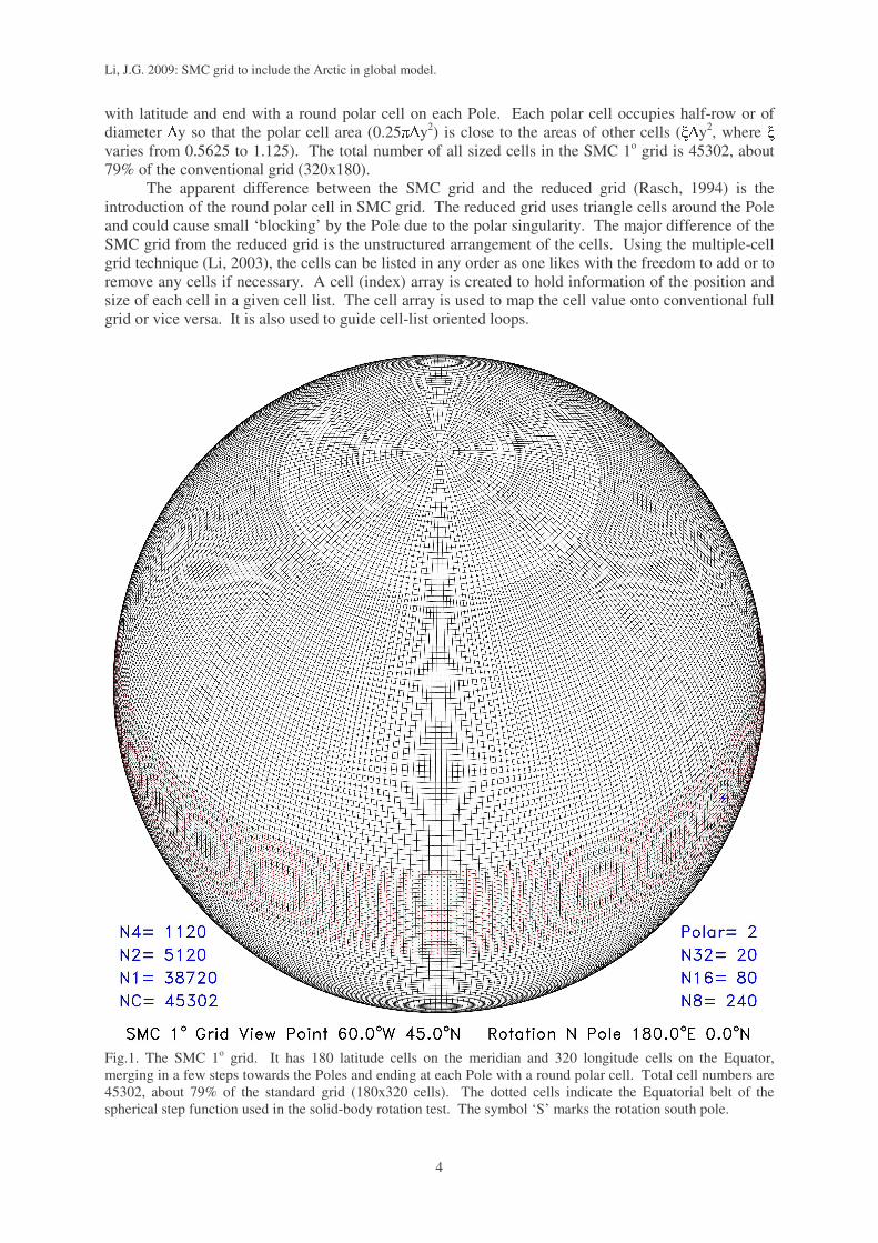
� � � k. Fig.1 illustrates the global SMC grid derived from a conventional lat-lon grid at � � = 1º and � � = 1.125º resolution. On the Equator there are 320 longitudinal cells and they merge in a few steps

Li, J.G. 2009: SMC grid to include the Arctic in global model.

4

with latitude and end with a round polar cell on each Pole. Each polar cell occupies half-row or of diameter � y so that the polar cell area (0.25� � y2) is close to the areas of other cells (

�� y2, where

�

varies from 0.5625 to 1.125). The total number of all sized cells in the SMC 1o grid is 45302, about 79% of the conventional grid (320x180). The apparent difference between the SMC grid and the reduced grid (Rasch, 1994) is the introduction of the round polar cell in SMC grid. The reduced grid uses triangle cells around the Pole and could cause small ‘blocking’ by the Pole due to the polar singularity. The major difference of the SMC grid from the reduced grid is the unstructured arrangement of the cells. Using the multiple-cell grid technique (Li, 2003), the cells can be listed in any order as one likes with the freedom to add or to remove any cells if necessary. A cell (index) array is created to hold information of the position and size of each cell in a given cell list. The cell array is used to map the cell value onto conventional full grid or vice versa. It is also used to guide cell-list oriented loops.

Fig.1. The SMC 1o grid. It has 180 latitude cells on the meridian and 320 longitude cells on the Equator, merging in a few steps towards the Poles and ending at each Pole with a round polar cell. Total cell numbers are 45302, about 79% of the standard grid (180x320 cells). The dotted cells indicate the Equatorial belt of the spherical step function used in the solid-body rotation test. The symbol ‘S’ marks the rotation south pole.

Proc. 11th WHF & 2nd CH Symposium. 18-23 Oct 2009, Halifax, Canada.

5

Fig.2. Solid-body rotation of a spherical step function on the SMC 1o grid as viewed in Fig.1. The rotation pole is on the Equator and the rotation speed is 1º per 3 time steps. The rectangular cell shape of the SMC grid is one major advantage over other unstructured grids, such as the triangle cells used by finite element grids (Hanert et al., 2004), the hexagon cells used by the spherical geodesic grid (Lipscomb and Ringler, 2005) and the conformal octagon approach (Purser and Rancis, 1997). The rectangular cells ensure finite difference schemes can be applied directly on the SMC grid as on the conventional lat-lon grid. They also provide a straight-forward mapping onto the conventional lat-lon grid. This is quite convenient if data exchange is required between the two grids. Even for fluxes cross the size-changing parallels, there is no need for any special treatment if each merged cell is considered to be two identical sub-cells of the pre-merging size. In numerical code the merged cell value is used directly in flux calculation as if its cell centre is still aligned along the meridian with the cells on the other side of the size-changing parallel. Two UNO advection schemes of 2nd (UNO2) and 3rd (UNO3) order accuracy (Li, 2008) are implemented on the SMC grid. They are derived by combining existing advection schemes in

Li, J.G. 2009: SMC grid to include the Arctic in global model.

6

different monotonic regions. UNO2 is an extension of the MINMOD scheme (Roe, 1985). UNO3 follows the ULTIMATE QUICKEST scheme (Leonard, 1991) to use a 3rd order scheme (Takacs, 1985) as its central part but replaces the flux limiters with a doubled MINMOD scheme. An advective-conservative hybrid operator (Leonard et al., 1996) is used to extend them to multi-dimensions for reduction of time-splitting error. Classical numerical tests have demonstrated that the UNO2/3 schemes are non-oscillatory, conservative, shape-preserving, and faster than their classical counterparts. As the UNO schemes are given in the so-called Upstream-Centre-Downstream (UCD) notation, their implementation on the SMC grid requires the knowledge of the immediate two cells on each side of a given cell face for evaluation of its flux. The neighbouring cell information can be pre-processed with the aid of the cell array and stored in a face array, which serves as pointers to link the face flux to its donor and recipient cells. For the given SMC 1o grid in Fig.1, there are 45300 U-faces (to which the u velocity component is normal) and 45620 V-faces (to which � is normal). Cell face widths are included in the flux evaluation to facilitate the varying cell-size with latitude. A temporary variable is used to hold all fluxes (or net flux) into one cell before all flux evaluations are completed. Cell values are updated in a separate cell loop with the net flux variables. As a result the two fluxes into the same merged cell above one size-changing parallel will be automatically added up at cell value update. This also makes the polar cell blend in smoothly with other cell update except its unique cell area and the sum of 10 V-fluxes given in (3) for its net flux. The east and west cyclic boundary condition used in the global lat-lon grid is naturally incorporated into the face array and the south and north boundaries have disappeared in the SMC grid as they merge into the polar cells. So the global transport of a scalar variable on the 2-D SMC grid does not need any boundary condition. This is an extra favour for optimization. 3. Solid-body rotation tests A solid-body rotation velocity field is used to demonstrate advection on the SMC grid. If the rotation pole is at (� P, � P) and the constant angular speed is � , the longitudinal and latitudinal velocity components of this solid-body rotation flow is given by

( )[ ]

( ) PP

P

r

ru

ϕπαλλαωυλλϕαϕαω

−≡−=−−=

2,sinsincossinsincoscos

(4)

The angular velocity � is set to be 10º per hour or the rotation period to be 36 hrs. Time step is set to be 120 s and the maximum Courant number is about 0.603. A full cycle around the sphere then takes 1080 time steps. The initial condition is a spherical step function (SSF), which is constructed by setting all cell values to be 1.0 unit except a stripe of 21 latitude cells wide around the Equator, which are set to be 5.0 unit high. Cells within the 5-unit stripe are marked by dots in Fig.1. The rotation pole is chosen on the Equator ( � = � /2) at

�P = � and the ‘S’ mark in Fig.1 indicates the rotation south pole. The

initial SSF field is shown in the top-left panel of Fig.2 (t = 0 hr) with exactly the same projection as in Fig.1. The SSF range is indicated by the maximum (Cmx = 5.0) and minimum (Cmn = 1.0) cell values printed on the lower-left corner of the panel. The colour keys are 40 levels per unit or a resolution of 0.025 unit. There are 256 colour levels in total, ranging from -0.10 to 6.3 unit. Each cell value is displayed by rounding it to the nearest colour level. Because the initial SSF has only two different values (the 1-unit background and the 5-unit stripe), it is displayed in two colours in the top-left panel of Fig.2. The SSF has the following two advantages for advection test on the sphere: Firstly, the SSF along each meridian resembles the 1-D step function, which is widely used in 1-D advection tests. The step edges are very sensitive to advection scheme oscillations and the uniform one unit background and 5-unit flat stripe would wrinkle up if there was any oscillation. The other advantage of the SSF for spherical solid-body rotation test is that the circular stripe will sweep over the full sphere and demonstrate whether it passes every cell smoothly without incurring any ripples. The upper-right panel in Fig.2 shows the solid-body rotation result with UNO3 scheme after t = 3 hr or 30º rotation. Its obvious difference from the initial condition (top-left panel) is the rounded

Proc. 11th WHF & 2nd CH Symposium. 18-23 Oct 2009, Halifax, Canada.

7

edges of the raised stripe. The initial steep step to the background is smoothed by the numerical diffusion, resulting in a continuous transition zone from the stripe top (5 unit) to the background (1 unit). This transition zone is illustrated by the intermediate colours between unit 1 and unit 5. Also note that the maximum and minimum values are 5.0070 and 0.9962 unit now, indicating a very small oscillation of the UNO3 scheme on the spherical grid. This might be attributed to the distortion of the cell shape from the rectangular shape. In fact, the oscillation is larger at high latitude than near the Equator as revealed by close examination. This can be further illustrated by the t = 9 hr result (lower-right panel in Fig.2) when the initial equatorial stripe has been rotated 90o to cover the Poles. The maximum value is 5.0150 unit by now, the largest value in the whole test. Close examination confirms that the extreme values are in the polar region near the stripe edges. Note that the polar cells are at the middle of the stripe now and their values are exactly 5.0 unit as the 20 cells surrounding them. This implies that the SSF passes through the size-changing parallels and the polar cells smoothly without any ripples. The bottom-left panel in Fig.2 shows the solid-body rotation result after one full cycle at t = 36 hr. The maximum and minimum values (5.0050 and 0.9969) indicate that the small oscillation at the stripe edges persists but smaller than that at the crossing Pole position (lower-right panel). By then the stripe has returned back to its initial position and it is apparently identical to the initial one (top-left panel) except its rounded stripe edges. Direct comparison of this result with the initial SSF can reveal the quality of the advection on the SMC grid. Following Williamson et al. (1992), a normalised rms (NRMS) error is used here to quantify the assessment and it is defined as

( ) ( )[ ] 2122�� −= i

refii

refi

ni AANRMS ψψψ (5)

where the summation is over all cells, Ai is the area of the i-th cell and � ref is the reference field. For this SSF solid-body rotation test, the reference field is simply chosen to be the initial SSF or � 0. The one-cycle (1080 time steps) NRMS error for rotation of the SSF on the SMC grid with the UNO3 scheme is 0.1624. Using the UNO2 scheme on the SMC grid for rotation of the same SSF shows very similar result except that the smoothing is slightly stronger than the UNO3 scheme. The NRMS value for the UNO2 scheme is 0.2161, slightly larger than the UNO3 one (0.1624). Considering that UNO2 scheme is much faster than UNO3, the small loss of accuracy is worthwhile especially if smoothing is required by other processes, like horizontal diffusion in ocean models (Killworth et al., 2003) and the smoothing term in ocean wave models (Tolman et al, 2002). 4. SMC grid for ocean surface The advantage of the unstructured SMC grid really manifests itself when some cells are removed from the full global grid. Fig.3 shows a global ocean surface SMC grid derived from the 40 km global lat-lon grid (� � = 0.375º and �

� = 0.5625º) of the Met Office operational atmospheric

model (Davies et al., 2005). The Polar Regions have been replaced by merged cells by the rule of the SMC grid, including a polar cell in the Arctic. All cells on land have been removed as they are not required in the ocean surface wave model. Although ice-covered ocean surface is treated as land in the wave model, the Arctic region is retained here for illustration of the SMC grid. There are 167944 sea cells in total, which is less than 55% of the conventional grid (640x480). Because the advection code on SMC grid for each cell face is identical to that on the conventional grid, the reduced cell number implies that the transportation on SMC grid will be about 55% less in computing cost than on the full lat-lon grid for each time step. If the relaxed time step is taken into account the transportation on SMC grid will be even faster than on the conventional grid. Another feature of the SMC grid is the unification of boundary condition with internal flux evaluation. Cell faces at the coastline are assumed to be bounded by two consecutive empty (zero) cells so that any wave energy transported into these zero cells will disappear and there is no wave energy out of these zero cells. This convenient setting conforms to the zero wave energy boundary condition at coastline used in ocean surface wave models and allows all the boundary cell faces to be treated as internal faces.

Li, J.G. 2009: SMC grid to include the Arctic in global model.

8

Fig.3. The SMC 40 km grid derived from conventional lat-lon grid, 640 longitude and 480 latitude cells, for a global ocean surface wave model, including the whole Arctic Ocean. Total cell number (167944) is less than 55% of the conventional grid (640x480).

Proc. 11th WHF & 2nd CH Symposium. 18-23 Oct 2009, Halifax, Canada.

9

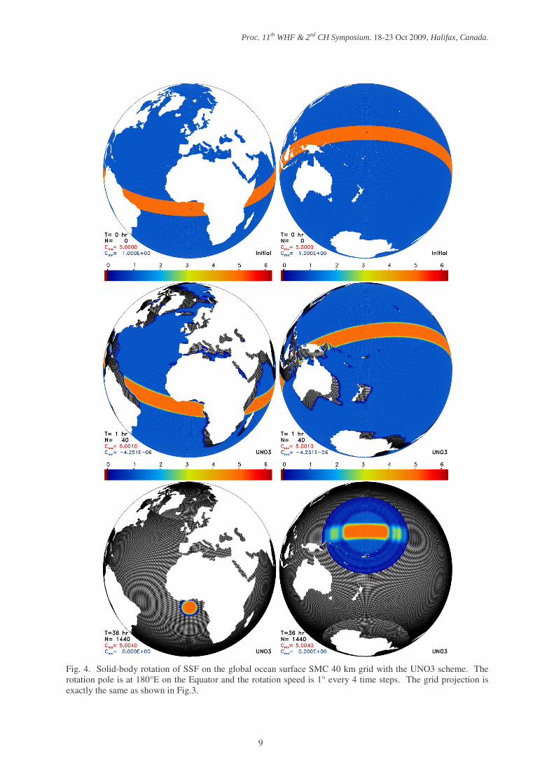
Fig. 4. Solid-body rotation of SSF on the global ocean surface SMC 40 km grid with the UNO3 scheme. The rotation pole is at 180°E on the Equator and the rotation speed is 1° every 4 time steps. The grid projection is exactly the same as shown in Fig.3.

Li, J.G. 2009: SMC grid to include the Arctic in global model.

10

If other boundary conditions are to be used, the cell numbers outside the boundary cell faces should be changed accordingly. For instance, the zero-gradient boundary condition may be implemented by simply setting the cell number outside the boundary face to be equal to the inside cell number. Pre-fixed boundary condition could be implemented by simply adding extra cells along the coastline. One extra benefit of using two consecutive zero-boundary cells is the completely blocking of wave energy by single-point islands. In conventional grid, wave energy can ‘leak’ through a single-point island due to the interpolation with neighbouring sea points. For SMC grid boundary faces, any single-point island is virtually extended into two zero cells beyond its boundary face so wave energy could not pass through it. Some small islands in the Mediterranean and east Pacific are visible as single-point islands in the SMC grid shown in Fig.5 and their blocking effect will be illustrated in the following rotation test. The solid-body rotation velocity is given by (4) with � P = 0 and � P = � in the ocean surface SMC grid test. The rotation pole is on the Equator in the middle of the Pacific, which provides a good test bed for the SSF rotation. The angular velocity � is also set to be 10º per hour or the rotation period to be 36 hrs. Time step is, however, reduced to 90 s as the grid length is reduced. A full cycle around the globe then takes 1440 time steps (1o every 4 steps). The maximum Courant number is about 0.840. The SSF is applied as the initial condition by first setting all sea points with an initial constant value of unit 1. The sea points within a stripe of 14 latitude cells on each side of the Equator (or 10.5° wide in latitude) are then raised to 5 units high. The initial SSF condition is shown in Fig.4 (top row marked t = 0 hr) and the cell value range is indicated by the min (Cmn = 1.0) and max (Cmx = 5.0) values. The white space represents land surface and small islands are now clearly visible by contrast to the background blue colour. The rotation poles are marked by the black ‘N’ and ‘S’ symbols on the initial equatorial stripe. The middle row in Fig.4 shows the transported field after 10º rotation (t = 1 hr) with the UNO3 scheme. The dark shadows off the coasts on the lee side indicate zero wave energy values as no wave energy comes out of the coastline. The complete-blocking of wave energy by islands is clearly visible by the dark shadows to the rear of them, including those single-point islands to the north of Australia. The edges of the raised stripe are rounded down by the implicit numerical diffusion, resulting in a transition zone in intermediate colours. Cell values in front of the coastline remain to be the initial background value as wave energy transported onto the coastline simply disappears (no reflection). The unclipped background and the stripe top remain uniformly flat, including the Arctic region. This result implies that the advection on the ocean surface SMC grid with the UNO3 scheme is smooth and efficient, including passing the polar cell, the size-changing parallels and the coastline boundary. Note that the max value is now slightly increased to 5.001 and the min value is a small negative value of -4.251E-6. This is in agreement with the previous test on the full globe SMC grid and confirms that the UNO3 scheme has very small oscillations on the spherical grid. These small negatives could be removed by a simple positive filter to ensure wave energy non-negative. The bottom two panels in Fig.4 show the results after a full cycle or 360º rotation with the UNO3 scheme (t = 36 hr). By now most of the initial SSF field has been clipped out by the coastline, leaving only one round disk on each hemisphere. The initial equatorial stripe has lost a few sections due to the land clipping. For this reason, it is no longer meaningful to evaluate the NRMS with reference to its initial condition. The surviving central section of the stripe retains its initial flat top of 5 unit high except the rounded edges, indicating that there is no apparent oscillation. The eastern disk (on the right panel) has pulled through a few islands, incurred a few grooves on the leeside. The grooves are gradually filled up with energy from neighbouring non-zero cells by the numerical diffusion as they are rotated away from the islands. The max value becomes 5.005 and the min value is now zero at double precision (64 bits). So the small oscillation is only about 0.1% (0.005/5.0). These results are quite satisfactory for ocean surface wave energy transportation. The efficient blocking by single-point islands is another desirable feature for the wave model. Similar SSF rotation is also done with the UNO2 scheme and the result is quite similar to the UNO3 one except that the UNO2 numerical smoothing is stronger. This is manifested by enlarged transition zone at the unclipped stripe edges and around the margin of the remaining disks. The shadow grooves on the leeside of small islands are shorter in the UNO2 case because of the enhanced filling effect by the numerical diffusion. Nevertheless, UNO2 scheme is accurate enough for ocean surface wave model because a strong explicit smoothing term is required in ocean wave models to

Proc. 11th WHF & 2nd CH Symposium. 18-23 Oct 2009, Halifax, Canada.

11

control the so called ‘garden sprinkler effect’ caused by the discrete representation of the 2-D ocean wave energy spectrum. The strong smoothing term makes the final wave energy field almost identical no matter the UNO2 or UNO3 scheme is used. Switching to the UNO2 scheme from the ULTIMATE QUICKEST 3rd order advection scheme (Leonard, 1991) in the WAVEWATCH III model (Tolman et al., 2002) has saved about 30% of advection computing time without any noticeable difference in the ocean wave energy. If the SMC grid is implemented, further saving on advection is expected. So the UNO2 scheme on this SMC grid will be ideal for global ocean surface wave models. The UNO3 scheme may be used for models where large numerical diffusion is not required. 5. Wave energy transport across the Arctic Ocean One difficulty to extend global ocean surface wave models into the Arctic is the underlying scalar assumption of directional spectral components. The increased curvature of the parallels at high latitudes renders the scalar assumption useless near the Pole. The longitudinal direction change of a given spectral bin becomes too large to be ignored within one time step. The difficulty stems from the choice of the local eastern direction as the spectral reference direction. This is, however, not necessary in the Arctic and the problem can be solved by simply introducing a fixed reference direction for the Arctic region. This means the Arctic region has to be treated separately from the other part of the global wave model. Fig. 5 illustrates the two parts of the global wave model above 50oN of the same SMC grid shown in Fig.3. The 66oN parallel is chosen as the boundary between the two parts to minimise the number of boundary cells. Within the 66oN parallel is the Arctic region where the wave spectral direction is defined from a fixed direction. Here the local east of a rotated grid (� P = � , � P = 0) is used rather than a truly fixed reference direction. The N Pole is on the rotated equator so the reference direction is well-defined for the polar cell. The direction defined by the rotated grid within the 66oN parallel is equivalent to the tropical directions used in the lat-lon grid so the validity of the scalar assumption is restored within the Arctic region by use of the rotated reference direction. Because of the different reference directions used by the two parts of the model domain, the wave spectra from the lower part could not be used directly for the Arctic part and vice versa. Hence proper links between the two parts are required for cross-boundary transport. This is achieved by introducing boundary conditions for the two parts. For the Arctic part, two rows just below the 66oN parallel are duplicated as extra cells in the SMC grid and their wave spectra are updated each time step with the corresponding cells in the lower part after rotated to the same reference direction. Similarly, two rows above the 66oN parallel are duplicated for the lower part and their spectra are updated with the Arctic cell spectra after proper rotation. Because the SMC grid uses unstructured list of cells, these extra boundary cells can be treated just like ordinary sea cells except their spectral update. The two parts are merged into a single cell loop and advection of each directional bin is calculated as in the old single reference direction case. With this polar modification, the whole Arctic Ocean can be included in global ocean surface wave models in case the Arctic ice disappears completely in future summers. The unstructured feature of the SMC grid makes this modification much easier than the conventional lat-lon grid. A pure advection test is done to demonstrate wave energy transport between the two reference direction parts. The wave spectral is assumed to be of 24 direction bins for a fixed frequency so each cell will hold 24 spectral components. The initial spectra are assumed to be zero except cells between 52o and 60oN in the lower part and cells above 86oN in the Arctic part. These non-zero cells are assigned with a typical wind-sea spectrum defined by

( ) ( )��� <−−

=Otherwise

forEE

,023,3cos2

0 ππθπθθ (6)

where E0 = 50/� is a constant and the integrated wave height �= θEdH is plotted in Fig.6 with a constant value of 5 units. The H is similar to the significant wave height used in wave models apart from a constant factor. The initial wave height field is shown in the upper-left panel of Fig.6. Note

Li, J.G. 2009: SMC grid to include the Arctic in global model.

12

the wind-sea spectrum (6) has a peak direction at 60o from its local reference direction. Because the two parts use different reference directions, the peak direction of the initial spectrum varies with longitude in the lower part as shown by the spectral roses in Fig. 6. Inside the Arctic part, however, the reference direction is nearly fixed at the map east so the initial spectral peak direction is nearly constant for all non-zero cells there. The wave speed and time step are set so that the wave travels at 1o every 4 time steps, resulting in a maximum Courant number of 0.884. The other three panels in Fig. 6 illustrate the wave energy transport with the UNO3 scheme on the SMC grid. The upper-right panel shows the simulated H field after 40 time steps or 10o great circle distance for each directional bin along its own moving direction. The initial Arctic round disk has spread out and the garden sprinkler effect is revealed by the directional fingers. This is a typical wind-sea pattern common in ocean surface wave models. The initial lower part circular stripe has crossed the boundary parallel into the Arctic part though some wave energy has disappeared at the coastlines. The crossing is obviously smooth in all the linking sections along the boundary parallel. Note the small portion of wave energy passing the Bering Strait into the Arctic. It will encounter with the initial Arctic wave and those entered from the opposite Greenland Sea in the later stage.

Fig. 5. The SMC 40 km grid above 50o N used for cross-Arctic wave energy transport test, showing the Arctic and lower parts (divided at 66oN) of different reference directions for wave energy spectra.

Proc. 11th WHF & 2nd CH Symposium. 18-23 Oct 2009, Halifax, Canada.

13

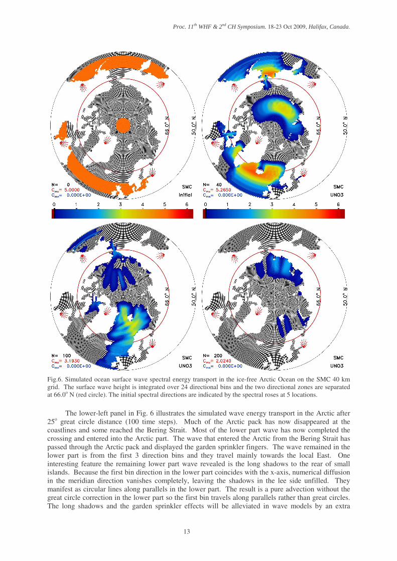
Fig.6. Simulated ocean surface wave spectral energy transport in the ice-free Arctic Ocean on the SMC 40 km grid. The surface wave height is integrated over 24 directional bins and the two directional zones are separated at 66.0o N (red circle). The initial spectral directions are indicated by the spectral roses at 5 locations. The lower-left panel in Fig. 6 illustrates the simulated wave energy transport in the Arctic after 25o great circle distance (100 time steps). Much of the Arctic pack has now disappeared at the coastlines and some reached the Bering Strait. Most of the lower part wave has now completed the crossing and entered into the Arctic part. The wave that entered the Arctic from the Bering Strait has passed through the Arctic pack and displayed the garden sprinkler fingers. The wave remained in the lower part is from the first 3 direction bins and they travel mainly towards the local East. One interesting feature the remaining lower part wave revealed is the long shadows to the rear of small islands. Because the first bin direction in the lower part coincides with the x-axis, numerical diffusion in the meridian direction vanishes completely, leaving the shadows in the lee side unfilled. They manifest as circular lines along parallels in the lower part. The result is a pure advection without the great circle correction in the lower part so the first bin travels along parallels rather than great circles. The long shadows and the garden sprinkler effects will be alleviated in wave models by an extra

Li, J.G. 2009: SMC grid to include the Arctic in global model.

14

smoothing term. The UNO3 scheme is chosen to illustrate these effects rather than mitigate them. For real wave models with the required smoothing term, the UNO2 scheme will be accurate enough. The lower-right panel in Fig. 6 illustrates the final stage of the lower part waves crossing the Arctic after 50o travelling from their initial positions. The fingers above the Pole are the waves from the Greenland Sea while these below the Pole come from the Bering Strait. They have passed each other and reached the opposite coastlines. The initial wave energy will disappear completely from this model domain after 70o great circle distance. This result is a typical wind-sea life cycle though other physical processes are not included. It confirms that the SMC grid with a fixed reference direction in the Arctic can be used to extend global wave model to high latitudes and even include the N Pole. 6. Summary and conclusions Second and third order upstream non-oscillatory (UNO) advection schemes are applied on a spherical multiple-cell (SMC) grid for global transport. The SMC grid is similar to the reduced grid to relax the CFL restriction of Eulerian advection time step on the conventional latitude-longitude (lat-lon) grid by merging the longitudinal cells towards the Poles. Round polar cells are introduced to remove the singularity of the standard lat-lon grid at the Poles. The mapping between the conventional lat-lon grid and the SMC grid is straightforward. Solid-body rotation of a spherical step function is used to test the UNO schemes on the SMC grid for global scalar transport. The unstructured feature of the SMC grid allows unused cells to be removed out of the advection calculation. Application of the SMC grid on the global ocean surface is used to demonstrate the flexibility of the SMC grid by removing all land points, reducing both memory and computing cost on a significant scale for global ocean surface wave models (55%). Ocean surface wave energy spectral transport in the Arctic is also demonstrated using a fixed reference direction for 2-D wave spectra. Numerical results indicate that the UNO3 scheme on the SMC grid is efficient and accurate enough for atmospheric and oceanic transport. The UNO2 scheme is fast and accurate enough for models where numerical diffusion is required, such as in the ocean surface wave model. They are easy to implement because the SMC grid retains the rectangular cells on the sphere as in the conventional lat-lon grid, which allows finite-difference schemes to be used directly. The SMC grid and the two UNO advection schemes are recommended for global atmospheric and oceanic tracer transportation. References Davies, T., M. J. P. Cullen, A. J. Malcolm, M. H. Mawson, A. Staniforth, A. A. White, N. Wood,

2005. A new dynamical core for the Met Office's global and regional modelling of the atmosphere. Q. J. R. Meteorol. Soc. 131, 1759-1782.

Golding, B. W., 1983. A wave prediction system for real-time sea state forecasting. Q. J. Roy. Meteoro. Soc., 109, 393-416.

Hanert, E., D. Y. Le Roux, V. Legat, E. Deleersnijder, 2004. Advection schemes for unstructured grid ocean modelling. Ocean Modelling 7, 39-58.

Hubbardk, M. E., N. Nikiforakis, 2003. A three-dimensional, adaptive, Godunov-type model for global atmospheric flows. Mon. Wea. Rev. 131, 1848-1864.

Janssen, P., 2004. The Interaction of ocean Waves and Wind, Cambridge University Press, 300 pp. Killworth, P. D., J. G. Li, D. Smeed, 2003. On the efficiency of statistical assimilation techniques in

the presence of model and data error. J. Geophys. Res. 108, C4 3113, doi:10.1029/2002JC001444. Kurihara, Y., 1965. Numerical integration of the primitive equations on a spherical grid. Mon. Wea.

Rev. 93, 399-415. Leonard, B. P., 1991. The ULTIMATE conservative difference scheme applied to unsteady one-

dimensional advection. Computer Methods Appl. Mech. Eng. 88, 17-74. Leonard, B. P., A. P. Lock, M. K. MacVean, 1996. Conservative explicit unrestricted-time-step multi-

dimensional constancy-preserving advection schemes. Mon. Wea. Rev. 124, 2588-2606.

Proc. 11th WHF & 2nd CH Symposium. 18-23 Oct 2009, Halifax, Canada.

15

Li, J. G., 2003. A multiple-cell flat-level model for atmospheric tracer dispersion over complex terrain. Boundary-Layer Meteorology, 107, 289-322.

Li, J. G., 2008. Upstream non-oscillatory advection schemes. Mon. Wea. Rev. 136, 4709-4729. Li, Y., J. S. Chang, 1996. A mass-conservative, positive-definite, and efficient Eulerian advection

scheme in spherical geometry and on a nonuniform grid system. J. Appl. Meteoro. 35, 1897-1913. Lipscomb, W. H., T. D. Ringler, 2005. An incremental remapping transport scheme on a spherical

geodesic grid. Mon. Wea. Rev. 133, 2335-2350. McDonald, A., J. R. Bates, 1989. Semi-Lagrangian integration of a gridpoint shallow water model on

the sphere. Mon. Wea. Rev. 117, 130-137. Nair, R. D., B. Machenhauer, 2002. The mass-conservative cell-integrated semi-Lagrangian advection

scheme on the sphere. Mon. Wea. Rev. 130, 649-667. Prather, M. J., M. McElroy, S. Wofsy, G. Russel, D. Rind, 1987. Chemistry of the global troposphere:

Fluorocarbons as tracers of air motion. J. Geophys. Res. 92, 6579-6613. Purser, R. J., M. Rancic, 1997. Conformal octagon: an attractive framework for global models offering

quasi-uniform regional enhancement of resolution. Meteorol. Atmos. Phys. 62, 33-48. Rasch, P. J., 1994. Conservative shape-preserving two-dimensional transport on a spherical reduced

grid. Mon. Wea. Rev., 122, 1337-1350. Robert, A., T. L. Yee, H. Ritchie, 1985. A semi-Lagrangian and semi-implicit numerical integration

scheme for multilevel atmospheric models. Mon. Wea. Rev. 113, 388-394. Roe, P. L., 1985. Large scale computations in fluid mechanics. Lectures in Applied Mathematics (E.

Engquist, S. Osher and R.J.C. Sommerville Eds.), 22, 163-193. Takacs, L. L., 1985. A two-step scheme for the advection equation with minimized dissipation and

dispersion errors. Mon. Wea. Rev. 113, 1050-1065. Tolman, H. L., B. Balasubramaniyan, L. D. Burroughs, D. V. Chalikov, Y. Y. Chao, H. S. Chen, V.

M. Gerald, 2002. Development and implementation of wind-generated ocean surface wave models at NCEP. Weather and Forecasting 17, 311-333.

WAMDI group, 1988. The WAM model - a third generation ocean wave prediction model. J. Phys. Oceanogr. 18, 1775-1810.

Wang, M., J. E. Overland, 2009: A sea ice free summer Arctic within 30 years? Geophys. Res. Lett., 36, L07502, DOI 10.1029/2009GL037820, 5 pp.

Williamson, D. L., J. B. Drake, J. J. Hack, R. Jakob, P. N. Swarztrauber, 1992. A standard test set for numerical approximations to the shallow-water equations in spherical geometry. J. Comput. Phys., 102, 221-224.

Zerroukat, M., N. Wood, A. Staniforth, 2004. SLICE-S: a Semi-Lagrangian inherently conserving and efficient scheme for transport problems on the sphere. Q. J. R. Meteoro. Soc. 130, 2649-2664.